CE 6504 - ndl.ethernet.edu.et

3/23/2020

1

CE 6504 Finite Elements Method in Structures

(Part 1)

AAiTMarch 2020

Bedilu Habte

AAiT – Civil Engineering – Bedilu Habte 2

Course Outline

1. Introduction 2. Preliminaries3. 1D (2-Node) Line Elements

Bar, Truss, Beam-elements, Shape functions

4. 2D ElementsPlane Stress and Plane Strain Problems

5. 3D ElementsTetrahedral, Hexahedral Elements

6. Plate Bending & Shells7. Further Issues

Modeling, Errors, Non-linearity


References

Finite Element Analysis (Text)By: S.S. BHAVIKATTI

Concepts and Applications of Finite Element AnalysisBy: Robert D. Cook, David S. Malkus and Michael E. Plesha

Finite Element Procedures in Engineering AnalysisBy: K.-J. Bathe

The Finite Element MethodO.C. Zienkiewicz

An Introduction to the Finite Element MethodBy: J. N. Reddy


Internet References:

FEM Primer Part 1 - 4Mike Barton & S. D. RajanArizona State Universityhttp://enpub.fulton.asu.edu/structures/FEMPrimer-Part1.ppt

Introduction to Finite Element MethodsDepartment of Aerospace Engineering SciencesUniversity of Colorado at Boulderhttp://www.colorado.edu/engineering/CAS/courses.d/IFEM.d/Home.html

Advanced Finite Element MethodsDepartment of Aerospace Engineering SciencesUniversity of Colorado at Boulderhttp://www.colorado.edu/engineering/CAS/courses.d/AFEM.d/Home.html

3/23/2020

2


I Introduction

What is FEM? Finite element method is a numerical method that generates approximate solutions to engineering problems which are usually expressed in terms of differential equations.

Used for stress analysis, heat transfer, fluid flow, electromagnetic etc.


• Use of several materials within the same structure, • complicated or discontinuous geometry, • complicated loading, etc,

makes the closed form (analytical) solution of structural problems very difficult.

One resorts to a numerical solution, the best of which is the FEM.

What is FEM?


Structure is partitioned into FINITE ELEMENTS – that are joined to each other at limited number of NODES

Behavior of an individual element can be described with a simple set of equations

Assembling the element equations, to a large set, is supposed to describe the behavior of the whole structure.

What is FEM?


Discretization Example

Find the circumference of a circle with a unit diameter – find the value of π.

Approximation with that of regular polygons:

3/23/2020

3


Solution:Let n be the number of sides of the inscribed or circumscribing polygon.

i) Inscribed polygonPerimeter p = n sin (180/n)

ii) Circumscribing polygonPerimeter p = n tan (180/n)



Estimated vs. exact value of π = 3.1415926536

No. of sides Inscribed polygon Error

3 2.5980762114 0.5435164422

4 2.8284271247 0.3131655288

8 3.0614674589 0.0801251947

16 3.1214451523 0.0201475013

32 3.1365484905 0.0050441630

64 3.1403311570 0.0012614966

128 3.1412772509 0.0003154027

1000 3.1415874859 0.0000051677

10000 3.1415926019 0.0000000517

100000 3.1415926531 0.0000000005

1000000 3.1415926536 0.0000000000



A formal mathematical theory for the FEM started some 60 years ago The steps in FEA are very similar to the method of the direct stiffness method in matrix structural analysis

The term finite element was first used by Clough in 1960.

The first book on the FEM by Zienkiewicz and Cheung was published in 1967.

In the late 1960s and early 1970s, the FEM was applied to a wide variety of engineering problems.

Brief History


The Pioneers – 1950 to 1962; Clough, Turner, Argyris, etc.; thought structural elements as a device to transmit forces (“force transducer”).

The Golden Age – 1962–1972; Zienkiewicz, Cheung, Martin, Carey etc.; thought discrete elements approximate continuum models (displacement formulation).

Brief History

3/23/2020

4


Consolidation – 1972 to mid 1980s; Hughes, Bathe Argyris, etc.; variational method, mixed formulation, error estimation.

Back to Basics – early 1980s to the present; Elements are kept simple but should provide answers of engineering accuracy with relatively coarse meshes.

Brief History


The 1970s advances in mathematical treatments, including the development of new elements, and convergence studies.

Most commercial FEM software packages originated in the 1970s and 1980s.

The FEM is one of the most important developments in computational methods to occur in the 20th century.

Brief History


Brief History


ANSYS

MSC/NASTRAN

ABAQUS

ADINA

ALGOR

NISA

COSMOS/M

STARDYNE

IMAGES-3D

Proprietary Software

3/23/2020

5


1. Discretize and Select Element Type

2. Select a Displacement Function

3. Define Strain/Displacement and Stress/Strain Relationships

4. Derive Element Stiffness Matrix & Eqs.

5. Assemble Equations and Introduce B.C.’s

6. Solve for the Unknown Degrees of Freedom

7. Solve for Element Stresses and Strains

8. Interpret the Results

Typical Steps in FEA Process


Common FEA Procedure for Structures

0. IdealizationThe given structure needs to be idealized based on engineering judgment. Identify the governing equation.

1. DiscretizationThe continuum system is disassembled into a number of small and manageable parts (finite elements).


2 – 4. Derivation of Element EquationsDerive the relationship between the unknown and given parameters at the nodes of the element.

5a. AssemblyAssembling the global stiffness matrix from the element stiffness matrices based on compatibility of displacements and equilibrium of forces.For example:


e e e

f k u


Displacement of a node is always the same for the adjoining elements and for the whole structure.

21

12

21

12

vvV

uuU

i

i


3/23/2020

6


For the whole structure, this process results in the masterstiffness equation:

The sum of the forces on each element of a particular node must balance the external force at that node.

Common FEA Procedure for Structures1 22 1

1 22 1

ix

iy

F f x f x

F f y f y

' ' 'K U F


5b. Introduce Boundary ConditionsAfter applying prescribed nodal displacements (and known external forces) to the master stiffness equation, the resulting equation becomes the modified master stiffness equation:


K U F


6. Solve for the primary unknowns

7/8. Compute other values of interestSecondary unknowns are determined using the known nodal displacements. Result interpretation.


1

U K F


1. Linear analysis: small deflection and elastic material properties.

2. Non-linear analysis: • Material non-linearity: small deflection and

non-linear material properties.• Geometric non-linearity: large deflection and

elastic material properties.• Both material and geometric non-linearity.

Types of FEA in Structures

3/23/2020

7


Advantages of Finite Element Analysis

• Models Bodies of Complex Shape

• Can Handle General Loading/Boundary Conditions

• Models Bodies Composed of Composite Materials

• Model is Easily Refined for Improved Accuracy by

Varying Element Size and Type (Approximation

Scheme)

• Time Dependent and Dynamic Effects Can Be Included

• Can Handle a Variety Nonlinear Effects


Common Sources of Error in FEA

• Domain Approximation

• Element Interpolation/Approximation

• Numerical Integration Errors

(Including Spatial and Time Integration)

• Computer Errors (Round-Off, Etc., )


Measures of Accuracy in FEA

Accuracy

Error = |(Exact Solution)-(FEM Solution)|

Convergence

Limit of Error as:

Number of Elements (h-convergence) or

Approximation Order (p-convergence)

Increases

Ideally, Error 0 as Number of Elements or Approximation Order is Higher


Numerical Methods

Several approaches can be used to transform the physical formulation of the problem to its finite element discrete analogue.

Ritz/ Galerkin methods – the physical formulation of the problem is known as a differential equation.

Variational formulation – the physical problem can be formulated as minimization of a functional.

3/23/2020

8


Variational Method cont.

• A mathematical model is a set of mathematical statements which attempts to describe a given physical system.


Strong Form (SF): A system of ordinary or partial differential equations in space and/or time, complemented by appropriate boundary conditions.

Weak Form (WF): A weighted integral equation that “relaxes” the strong form into a domain-averaging statement.

Variational Form (VF): A functional whose stationary conditions generate the weak and strong forms.

Variational Method cont.


Elasticity

x

xy

y

z

zy

zx xz

yz

xy

3D Stress block


Elasticity cont.

Stress Equilibrium Equations

3/23/2020

9


Elasticity cont.


Elasticity cont.

Strain – Displacement


Elasticity cont.

3D Stress – Strain Relationships


Bar Elements

(1) The longitudinal dimension or axial dimension is much larger that the transverse dimension(s). The intersection of a plane normal to the longitudinal dimension and the bar defines the cross sections.

(2) The bar resists an internal axial force along its longitudinal dimension.

3/23/2020

10


Bar Elements cont.


Bar Elements cont.


Bar Elements cont.

• It must be in equilibrium.• It must satisfy the elastic stress–strain law (Hooke’s law)

• The displacement field must be compatible.

• It must satisfy the strain–displacement equation.


Governing Equation

The governing differential equation of the bar element is given by

Pdx

duAE

u

conditionsboundary

qdx

duAE

dx

d

Lx

x

0

0

0

3/23/2020

11


Admissible displacement function is continuous over the length and satisfies any boundary condition:

Principles of Minimum Potential Energy – Of all

kinematically admissible displacement equations, those corresponding to equilibrium extermize the TPE. If the extremum is a minimum, the equilibrium state is stable.

Approximate Solution


Kinematically admissible Displacement Functions

those that satisfy the single-valued nature of displacements (compatibility) and the boundary conditions

Usually Polynomials

Continuous within element.

Inter-element compatibility. Prevent overlap or gaps.

Allow for rigid body displacement and constant strain.


Total Potential Energy (TPE)

Strain Energy (Internal

work)

Jima – Civil Engineering – Bedilu Habte

dVU

dVdU

dVddU

dzyxdU

WU

V

xx

V

ε

xx

xx

xx

p

x

2

1

0


External work of loads

Total Potential Energy

TPE


S

M

iiix

V

b

p

dfdSuTdVuXW

WU

1

ˆˆˆˆˆ

WdxAE x

L

xp 2

1

3/23/2020

12


Strain energy

External energy

Total potential energy

1

2

Total Potential Energy


AdxL

T 2

1

2Pu

22

1PuAdxΠ

L

T


Ritz-Method


Ritz-Method

Using the Ritz-method, approximate displacement function is obtained by:

Assume arbitrary displacement

Introduce this into the TPE functional

Performing differentiation and integration to obtain a function

Minimizing the resulting function

nn fafafa ...2211

niforda

d

i

,...,2,10


Ritz-Method

Consider the linear elastic one-dimensional rod with the force shown below

• The potential energy of this system is:

1

2

0

2

21 2udx

dx

duEAΠ

3/23/2020

13


Ritz-Method

Consider the polynomial function:

To be kinematically admissible u must satisfy the boundary conditions u = 0 at both (x = 0) and (x = 2)

Thus:

&


Ritz-Method

• TPE of this system becomes:

• Minimizing the TPE:

• Thus, an approximate u is given by:

• Rayleigh-Ritz method assumes trial functions over entire structure


Galerkin-Method

For the one-dimensional rod considered in the pervious example, the governing equation is:

The Galerkin method aims at setting the residual relative to a weighting function Wi, to zero. The weighting functions, Wi, are chosen from the basis functions used for constructing û (approximate displacement function).


Galerkin-Method

Using the Galerkin-method, approximate displacement function is obtained by:

The governing DE is written in residual form

Multiply this RES by weight function f and integrate and equate to zero

Perform differentiation and integration to obtain the approximate u

dx

duAE

dx

dRES

0 dxRfL

3/23/2020

14


Galerkin-MethodConsider the rod shown below

• Multiplying by Φ (weighting function) and integrating gives (by parts):


Galerkin-MethodThe function Φ is zero at (x = 0) and (x = 2)

and EA(du/dx) is the force in the rod, which equals 2 at (x = 1). Thus:

• Using the same polynomial function for u and Φ and if u1 and Φ1 are the values at (x = 1):

• Setting these and

E=A=1 in the integral:


Galerkin-MethodEquating the value in the bracket to zero and

performing the integral:

• In elasticity problems Galerkin’s method turns out to be the principle of virtual work.

43

1 u 2275.0 xxu


Bar Element

L

1

2

xx fd 11ˆ,ˆ

u,x

xx fd 22ˆ,ˆ

y

Y

X 0ˆ

ˆ

ˆ

ˆ

ˆ

ˆ

xd

udAE

xd

d

ATA

xd

ud

E

x

3/23/2020

15


Assumptions

The bar cannot resist shear forces.

That is:

Effects of transverse displacements are ignored.

Hooke’s law applies.

That is:

0ff y2y1

xx E


Select a Displacement Function

Assume a linear function.

No. of coefficients = No. of DOF

Written in matrix form:

Expressed as function of and

uxaau ˆˆ 21

2

1ˆ1ˆa

axu

LaddLaadLu

adaadu

xxx

xx

212212

11211

ˆˆ)(ˆ)(ˆ

ˆ)0(ˆ)0(ˆ

x1d x2d


Shape functions:

2x 1x1x

1x

2x

1x

1 2

2x

1 2

ˆ ˆd d ˆˆ ˆu x dL

dˆ ˆx xu 1

ˆL L d

du N N

d

Where :

ˆ ˆx xN 1 and N

L L


Shape Functions

N1 and N2 are called Shape Functions or Interpolation Functions. They express the shape of the assumed displacements.N1 =1 N2 =0 at node 1N1 =0 N2 =1 at node 2N1 + N2 =1 at any point

1 2

N1 N2

L

1 1


3/23/2020

16


Define Strain/Displacement and Stress/Strain Relationships


L

ddEE

L

dd

xd

ud

dxL

ddu

xx

xx

xxx

12

12

112

ˆˆ

ˆˆ

ˆ

ˆ

ˆˆˆˆ

ˆ

L

ddAEf

L

ddAEf

Af

xxx

xxx

122

211

ˆˆˆ

ˆˆˆ


Derive the Element Stiffness Matrix and Equations

Assemble Global Stiffness Matrix, apply BC and solve the Master stiffness equation for the unknown

displacements:


11

11ˆ

ˆ

ˆ

11

11

ˆ

ˆ

2

1

2

1

L

AEk

d

d

L

AE

f

f

x

x

x

x

FdK

fF

kK

N

e

e

N

e

e

1

)(

1

)(

ˆ

ˆ


Potential Energy Approach


dVU

dVddU

WU

V

xx

xx

p

2

1

S

M

iixixx

V

b dfdSuTdVuXW1

ˆˆˆˆˆ



V

b

S

xxxxx

L

xxp dvXudSTudfdfxdA ˆˆˆˆˆˆˆˆˆ2

12211

0

x

x

d

dd

L

x

L

xN

dNu

2

1

ˆ

ˆˆ

ˆˆ1

}ˆ{][ˆ

LLB

dB

dLL

x

x

11

ˆ

ˆ11

3/23/2020

17



[D] is the constitutive matrix(elasticity property matrix)

dBD

ED

D

x

xx

ˆ

V

b

S

xxxxx

L

xxp dvXudSTudfdfxdA ˆˆˆˆˆˆˆˆˆ2

2211

0



V

b

T

S

xT

TL

x

T

xp dvXudSTuPdxdA ˆˆˆˆˆˆ2

0

V

b

TT

S

x

TTT

LTTT

p

dvXNddSTNdPd

xddBDBdA

ˆˆˆˆˆ

ˆˆˆ2

0

V

b

T

S

x

T

TTTT

p

dvXNdSTNPf

fddBDBdAL

ˆˆ}{ˆ

ˆˆˆˆ2



xxxx

T

xxxx

x

xxx

TTT

fdfdfd

ddddL

EU

d

d

LLE

L

LddU

dBDBdU

2211

2221

212

*

2

121

*

*

ˆˆˆˆˆˆ

ˆˆˆ2ˆ

ˆ

ˆ111

1

ˆˆ

ˆˆ



0ˆˆ2ˆ22ˆ

0ˆˆ2ˆ22ˆ

2122

2

1212

1

xxx

x

p

xxx

x

p

fddL

EAL

d

fddL

EAL

d

1 1

2 2

ˆ ˆ1 1

ˆ ˆ1 1

x x

x x

T T

V

d fAE

L d f

k B D B dV D D

3/23/2020

18


Transformation Matrix (Local Global)

θS

θC

Let

sin

cos

fTf

dTd

d

d

d

d

CS

SC

CS

SC

d

d

d

d

y

x

y

x

y

x

y

x

ˆ

ˆ

00

00

00

00

ˆ

ˆ

ˆ

ˆ

2

2

1

1

2

2

1

1

CS

SC

CS

SC

T

00

00

00

00


Element stiffness equation in local coordinate:

Element stiffness matrixin the global coordinate:

y

x

y

x

y

x

y

x

d

d

d

d

L

AE

f

f

f

f

2

2

1

1

2

2

1

1

0000

0101

0000

0101

ˆ

ˆ

ˆ

ˆ

TkTk

dTkTf

TT

dTkTf

dTkfT

T

T

T

ˆ

ˆ

ˆ

ˆ

1

1


Obtain displacement function for the one-dimensional quadratic element with three nodes shown below.

Quadratic Bar Element

A quadratic displacement function:

No. of coefficients = No. of DOF

Written in matrix form:

3

2

12ˆˆ1ˆ

a

aa

xxu

2321ˆˆˆ xaxaau


3

2ˆ

20ˆ

1

2ˆ

ˆ

ˆ

ˆ

du

du

du

Lx

x

Lx

42

42

232

13

12

232

11

LaLaad

ad

LaLaad

2

3 12 3 2 1 2

12 2 2

22 2 2

3

ˆˆ ˆ 2 2

ˆ ˆ ˆ ˆ ˆ2 4 21

d d xu d x d d d

L L

dx x x x x

dL L L L L

d

1

1 2 3 2

3

d

N N N d

d

3/23/2020

19


Quadratic Shape Functions

N1 =1 N2 = N3 =0 at node 1N2 =1 N1 = N3 =0 at node 2N3 =1 N1 = N2 =0 at node 3

N1 + N2 + N3 = 1 at any point


PROPERTIES OF THE SHAPE FUNCTIONS

The shape function at any node has a value of 1 at that node and a value of zero at ALL other nodes.

x1 x2

1 1

Check

x

21

2 1

x -xN (x)

x x

1

2

2 1

x-xN (x)

x x

0xx

x-x)x(xNand

1xx

x-x)x(xN

xx

x-x(x)N

12

2221

12

1211

12

21


Compatibility: The displacement approximation is continuous across element boundaries

x1 x2El #1 x3El #2

Hence the displacement approximation is continuous across elements


Writing shape functions (without deriving):

x1 x2El #1

1 1

The Kronecker delta property (the shape function at any node has value of 1 at that node and a value of zero at all other nodes)

Notice that the length of the element = x2-x1

Node at which N1 is 0

The denominator is the numerator evaluated at the node itself

21

2 1

1 1

2

1 2 2 1

x -xN ( x )

x - x

x -x x -xN ( x )

x - x x -x

x

21

2 1

x -xN (x )

x x

12

2 1

x-xN (x)

x x

3/23/2020

20


3-Node bar element: varying quadratically inside the bar

3231

213

2321

312

1312

321

x-xx-x

x-xx-x(x)N

x-xx-x

x-xx-x(x)N

x-xx-x

x-xx-x(x)N

xx1 x2

(x)N1(x)N3

x3

1

(x)N2

1 1x 2 2x 3 3xu(x) N (x)d N (x)d N (x)d

This is a quadratic finite element in 1D and it has three nodes and three associated shape functions per element.


Writing shape functions for higher DOFs:


STRAIN and STRESS WITHIN EACH ELEMENT

From equation (1), the displacement within each element

The strain in the bar

Hence

(2)

The matrix B is known as the “strain-displacement matrix”

( x ) = N d

dx

dε

d Nε d B d

dx

d NB

dx


For a linear finite element

Hence

For a linear bar element, strain is a constant within the element.

2 1 2 1 2 1

-1 1 1B 1 1

x x x x x x

2 11 2

2 1 2 1

x -x x -xN N (x ) N (x )

x x x x

1 x

2 x2 1 2 1

2 x 1 x

2 1

d- 1 1ε B d

dx x x x

d - d

x x

3/23/2020

21


x1 x2

El #1

Displacement is linear

Strain is constant

The stress in the bar

Inside the element, the approximate stress is

The stiffness matrix

2xd

1xd x

0 1(x ) a a x

2 x 1 x

2 1

d -dε =

x x

d uE ε = E

d x

E B d

T

V

k B E B d V


O1

2P

x1

x2 = x1 + L

L

Mapped on the following Natural Coordinate

Natural Coordinates

-1P

2

1


2 Node Linear Element

1

N1

1

N2

x

x2-xN1 = -----------

x2-x1

1 - N1 = -----------

2

x-x1N2 = ----------

x2-x1

+ 1N2 = ---------

2

x1-1

x21

L

x


1 23

1 23

1 23

3 Node Quadratic Element

x21

123

x1-1

x30

2

32

2

31

13

2

23

3

21

12

2

13

3

12

21

11

-1

1

-1-

xx

x-x

xx

x-xN

2

1

1

-

2

-1-

xx

x-x

xx

x-xN

2

1

1

-

2

-1

xx

x-x

xx

x-xN

3/23/2020

22


Beam Theory – Terminology

A general beam is a bar-like member designed to resist a combination of loading actions such as biaxial bending, transverse shears, axial stretching or compression, and possibly torsion.

If the beam is subject primarily to bending and axial forces, it is called a beam-column.

A beam is straight if its longitudinal axis is straight. It is prismatic if its cross section is constant.

A spatial beam supports transverse loads that can act on arbitrary directions along the cross section.

A plane beam resists primarily transverse loading on a preferred longitudinal plane.


Mathematical Models

One-dimensional mathematical models of structural beams are constructed on the basis of beam theories.

The simplest and best known models for straight, prismatic beams are based on the:

Bernoulli-Euler theory (also called classical beam theory or engineering beam theory)

Timoshenko beam theory


Beam Theory – Kinematics


Beam Theory – Terminology

3/23/2020

23


Bernoulli-Euler Model


Mathematical Model

Total Potential Energy of Beam Members


Bernoulli-Euler Beam Theory


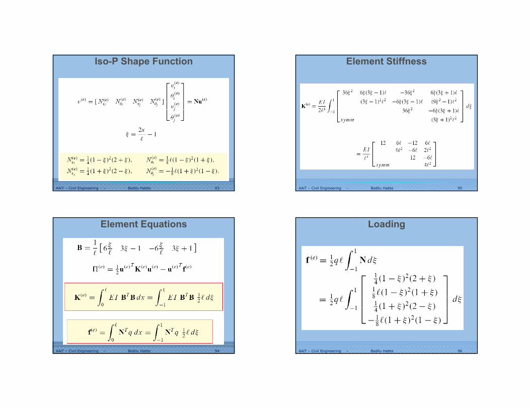
Iso-P Shape Function

3/23/2020

24


Iso-P Shape Function


Element Equations


Element Stiffness


Loading

3/23/2020

25


General 3D Frame Element


L

EI

L

EI

L

EI

L

EIL

EI

L

EI

L

EI

L

EIL

GI

L

GIL

EI

L

EI

L

EI

L

EIL

EI

L

EI

L

EI

L

EIL

EA

L

EAL

EI

L

EI

L

EI

L

EIL

EI

L

EI

L

EI

L

EIL

GI

L

GIL

EI

L

EI

L

EI

L

EIL

EI

L

EI

L

EI

L

EIL

EA

L

EA

K

zzzz

yyyy

xx

yyyy

zzzz

xx

zzzz

yyyy

xx

yyyy

zzzz

xx

ji

4000

60

2000

60

04

06

0002

06

00

0000000000

06

012

0006

012

00

6000

120

6000

120

0000000000

2000

60

4000

60

02

06

0004

06

00

0000000000

06

012

0006

012

00

6000

120

6000

120

0000000000

][

22

22

2323

2323

22

22

2323

2323

Stiffness of a 3D Frame Element

3/23/2020 98


Example 1 – Analyse the plane truss


Example 1

3/23/2020

26


Example 2 – Analyze the Plane Frame


Example 2 – Element and node numbering


Example 2 – Boundary Condition & Solve


Documents

CE 6504 - ndl.ethernet.edu.et