発展方程式の数値解析 II. Keller-Segel の走化性モデ …発展方程式の数値解析 II. Keller-Segelの走化性モデルと有限体積法齊藤宣一(Norikazu SAITO)

発展方程式の数値解析II. Keller-Segelの走化性モデルと有限体積法

齊藤宣一 (Norikazu SAITO)

東京大学大学院数理科学研究科

2011年 8月 27日発展方程式若手セミナー

http://www.infsup.jp/saito/materials/110827tsukuba2.pdf

N. Saito (UT) Evolution Equations II August 27, 2011 1 / 32

目次

1 Keller-Segel system modeling chemotaxis

2 A remark on the positivity of a solution of a convection-diffusion equation

3 Introduction to the finite volume method

4 Numerical examples


§1. Keller-Segelの走化性モデル


Keller-Segel の走化性モデル

E. F. Keller & L. A. Segel : J. Theor. Biol. 26 (1970)

Mathematical models to describe the aggregation of cellular slime molds which move preferentially to relatively

high concentrations of a chemical secreted by themselves

u = u(x, t): the cell density of the slime molds;

v = v(x, t): the concentration of the chemical substance;

∇ϕ(v): the velocity of u due to chemotaxis.


Keller-Segel の走化性モデルE. F. Keller & L. A. Segel : J. Theor. Biol. 26 (1970)






u

Diffusion








f(v)

u

uu

Chemotaxis








u v

f(v)

Creation of field


Diffusion Chemotaxis Creation of field


Diffusion Chemotaxis Creation of field

Rem: Flux of u is given by j = −Du∇u + u∇ϕ(v).

Keller-Segel system:

ut = −∇ · j = ∇ · (Du∇u − u∇ϕ(v))

kvt = Dv∆v + g(u, v)

Boundary conditions:

−j · ν = Du

∂u

∂ν− u

∂ϕ(v)

∂ν= 0

∂v

∂ν= 0.


Keller-Segel system (E. F. Keller & L. A. Segel 1970)

ut = ∇ · (Du∇u − u∇ϕ(v)) in Ω × (0, T ),

kvt = Dv∆v − k1v + k2u in Ω × (0, T ),

∂u

∂ν= 0,

∂v

∂ν= 0 on ∂Ω × (0, T ),

u|t=0 = u0, v|t=0 = v0 on Ω

(KS)

Ω: bounded domain in Rd (d = 2, 3)

Mathematical model for aggregation phenomenon of slime molds resultingfrom their chemotactic features

u density of the cellular slime molds;v concentration of the chemical substance secreted by molds;Du, Dv diffusion coefficients, k relaxation time (≥ 0) and k1v − k2u ratio ofgeneration/extinction.ϕ(v) sensitive function (ϕ : R → R smooth and non-deceasing),

Conservation laws: positivity and total mass; ‖u(t)‖L1 = ‖u0‖L1 .

The solution may blow up. (It depends on ‖u0‖L1 and d.)


Well-posedness

Ω and u0(x) are “smooth”

⇒ ∃(u, v): unique classical solution on [0, T ], T ∈ (0, Tmax).

Tmax: the supremum of the existence time;

Tmax = ∞ ⇒ global existence;Tmax < ∞ ⇒ blow up (in finite time) i.e., lim

t→Tmax

‖u(t)‖L∞ = +∞.

Horstmann (survey, 2003, 2004), Suzuki & Senba (book, 2004), Suzuki(book, 2005), ......

Example. Assume k = 0.

Ω ⊂ R1 ⇒ Tmax = +∞.

Ω ⊂ R2,

(i) ‖u0‖L1(Ω) < 4πλ−1 ⇒ Tmax = ∞;

(ii) ‖u0‖L1(Ω) > 8πλ−1 and

∫

Ω

|x − x0|2u0(x) dx 1 for some x0 ∈ Ω. ⇒

Tmax < ∞.


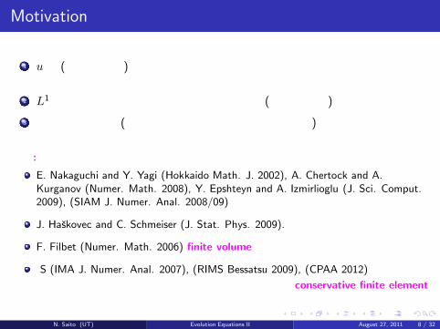
Motivation

1 uが (凝集による)集中化を相当におこしても，安定に計算を遂行できる数値計算スキームの提案

2 L1 ノルムの保存や自由エネルギーの保存を (できるだけ)再現3 理論的な裏付け (安定性・収束解析，陽的な誤差評価)

注意:

E. Nakaguchi and Y. Yagi (Hokkaido Math. J. 2002), A. Chertock and A.Kurganov (Numer. Math. 2008), Y. Epshteyn and A. Izmirlioglu (J. Sci. Comput.2009), (SIAM J. Numer. Anal. 2008/09)

J. Haskovec and C. Schmeiser (J. Stat. Phys. 2009).

F. Filbet (Numer. Math. 2006) finite volume

S (IMA J. Numer. Anal. 2007), (RIMS Bessatsu 2009), (CPAA 2012)

conservative finite element


§2. A remark on the positivity of a numericalsolution of a convection-diffusion equation


Illustration of the issue

Model problem: u(x, t), b(x, t) ≥ 0: 1-periodic functions in x

ut = uxx − (b(x, t)u)x (x ∈ [0, 1), 0 < t < T )

Positivity u(x, 0) ≥ 0, 6≡ 0 ⇒ u(x, t) > 0 (t > 0)

Finite difference method:

xi = ih (h = 1/N)，tn = τ1 + τ2 + · · · + τn: Grid points;

bni = b(xi, tn);

uni ≈ u(xi, tn): finite difference approximation.

forward Euler = central difference + central difference

uni − un−1

i

τn

=un−1

i−1 − 2un−1i + un−1

i+1

h2−

bn−1i+1 un−1

i+1 − bn−1i−1 un−1

i−1

2h


Numerical example

b(x, t) = 4(1 + cos 2πx)(1 + t)2，h = 2−5，τj = 0.4 · h2

0

0.2

0.4

0.6

0.8

0 0.5

1 1.5

2 2.5

3 3.5

4

0

2

4

0 ≤ tn ≤ 4.0


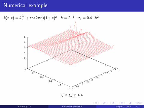
Numerical example

b(x, t) = 4(1 + cos 2πx)(1 + t)2，h = 2−5，τj = 0.4 · h2

0

0.2

0.4

0.6

0.8

1 0 0.5

1 1.5

2 2.5

3 3.5

4 4.5

-8

-4

0

4

8

0 ≤ tn ≤ 4.4


Numerical example

b(x, t) = 4(1 + cos 2πx)(1 + t)2，h = 2−5，τj = 0.4 · h2

0

0.2

0.4

0.6

0.8

1 4.37 4.375

4.38 4.385

4.39 4.395

4.4

-80

-40

0

40

80

4.37 ≤ tn ≤ 4.4


Numerical example

b(x, t) = 4(1 + cos 2πx)(1 + t)2，h = 2−5，τj = 0.4 · h2

-50

-40

-30

-20

-10

0

10

20

30

40

50

0 0.2 0.4 0.6 0.8 1

u-ax

is

x-axis

4.37 ≤ tn ≤ 4.4 (another view-point)


Consideration

Finite difference scheme(

λn = τn/h2)

⇔

uni = (1 − 2λn)un−1

i +(

λn +τn

2hbn−1i−1

)

un−1i−1 +

(

λn −τn

2hbn−1i+1

)

un−1i+1

Non-negativity (*) un−1i ≥ 0 (∀i) ⇒ un

i ≥ 0 (∀i)

A sufficient condition:

(· · · ) ≥ 0，(· · · ) ≥ 0，(· · · ) ≥ 0 ⇒ (*)

h ≤1

2βn−1⇒ (*).

(

βn = max1≤i≤N

bni

)

Before computation, we have to choose h satisfying:

h ≤1

2βT

, βT = max0≤tn≤T

βn.


Upwind finite difference scheme

forward Euler = central difference＋ upwind difference

uni − un−1

i

τn

=un−1

i−1 − 2un−1i + un−1

i+1

h2−

bn−1i un−1

i − bn−1i−1 un−1

i−1

h

⇔

uni =

(

1 − 2λn −τn

hbn−1i

)

un−1i +

(

λn +τn

hbn−1i−1

)

un−1i−1 + λnun−1

i+1

A sufficient condition： τn ≤h2

2 + hβn−1⇒ (*).

In each time step, we re-choose τn to satisfy the above condition.

Extension to d ≥ 2 and arbitrary Ω

FEM; Tabata (1977), Heinrich et al. (1977) → flow problems.In general, the upwind FEM destroys the conservation of mass.

Conservative numerical schemes;

FEM; Baba-Tabata upwinding (1981),Finite volume method (FVM), .....


§3. Introduction to the finite volume method


Convection-diffusion problem (model problem)

Find a function u = u(x, t) of (x, t) ∈ Ω × [0, T ] satisfying

ut −∇ · (∇u − bu) = f in Ω × (0, T ),

u = g on ∂Ω × (0, T ),

u|t=0 = u0 on Ω,

(1)

Ω: bounded polygonal/smooth domain in R2

Remark: It is straightforward to extend the results to the 3D case; we needsome trivial modifications.

T : positive constant

f : Ω × (0, T ) → R, g : ∂Ω × (0, T ) → R, u0 : Ω → R: smooth

b : Ω × (0, T ) → R2 smooth


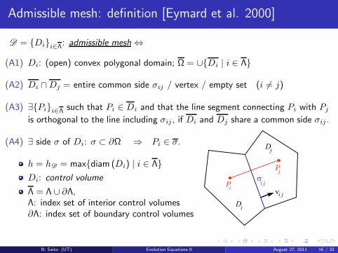
Admissible mesh: definition [Eymard et al. 2000]

D = Dii∈Λ: admissible mesh ⇔

(A1) Di: (open) convex polygonal domain; Ω = ∪Di | i ∈ Λ

(A2) Di ∩ Dj = entire common side σij / vertex / empty set (i 6= j)

(A3) ∃Pii∈Λ such that Pi ∈ Di and that the line segment connecting Pi with Pj

is orthogonal to the line including σij , if Di and Dj share a common side σij .

(A4) ∃ side σ of Di: σ ⊂ ∂Ω ⇒ Pi ∈ σ.

h = hD = maxdiam (Di) | i ∈ Λ

Di: control volume

Λ = Λ ∪ ∂Λ,Λ: index set of interior control volumes∂Λ: index set of boundary control volumes

Pi

jP

i js

Di

Dj

ni j


Admissible mesh: examples (acute triangulations)

iP

PC

circumcentric domain(PC = circumcenter)

iP

GP

barycentric domain(PG = barycenter)



acute triangulation admissible mesh

Lemma: The circumcentric dual mesh of an acute triangulation is an admissiblemesh.

Remark: The barycentric dual mesh does not imply an admissible mesh ingeneral.



acute triangulation admissible mesh

Lemma: The circumcentric dual mesh of an acute triangulation is an admissiblemesh.

Remark: The barycentric dual mesh does not imply an admissible mesh ingeneral.


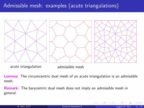
Admissible mesh: examples (Voronoi diagram)

Voronoi diagram Voronoi diagram


Admissible mesh: examples (Voronoi diagram)

admissible mesh admissible mesh

Lemma: A Voronoi diagram implies an admissible mesh if the number of pointsPi which are located on ∂Ω is large enough.


Definitions

Piecewise constant functions:

Xh = vh ∈ L∞(Ω) | vh|Di= Const. (i ∈ Λ)

Vh = vh ∈ Xh | vh|Di= 0 (i ∈ ∂Λ)

τij =mij

dij

transmissibility

mij = length of σij

dij = |Pi − Pj |

mi = area of Di

Pi

jP

i js

Di

Dj

ni j


Approximation of the diffusion part

∫

Di

(−∆u) dx = −

∫

∂Di

∇u · νi dS

= −∑

j∈Λi

∫

σij

∇u · νij dS

≈ −∑

j∈Λi

∫

σij

u(Pj) − u(Pi)

dij

dS

= −∑

j∈Λi

τij(u(Pj) − u(Pi)).

P5

7P

5,7s

D5

D7

D2

D4

5,2s

5,4s

τij =mij

dij

, mij = length of σij , dij = |Pi − Pj |

Λi = j ∈ Λ | Pi and Pj share the entire common side σij

(Λ5 = 2, 4, 7)


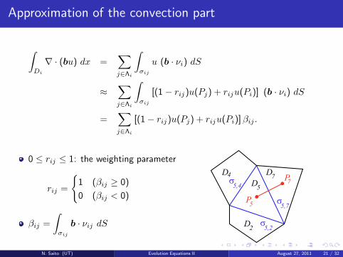
Approximation of the convection part

∫

Di

∇ · (bu) dx =∑

j∈Λi

∫

σij

u (b · νi) dS

≈∑

j∈Λi

∫

σij

[(1 − rij)u(Pj) + riju(Pi)] (b · νi) dS

=∑

j∈Λi

[(1 − rij)u(Pj) + riju(Pi)] βij .

0 ≤ rij ≤ 1: the weighting parameter

rij =

1 (βij ≥ 0)

0 (βij < 0)

βij =

∫

σij

b · νij dS

P5

7P

5,7s

D5

D7

D2

D4

5,2s

5,4s


Finite volume scheme

Find unh

nn=0 ⊂ Xh satisfying

uni − un−1

i

∆tmi −

∑

j∈Λi

τij(unj − un

i )

+∑

j∈Λi

βnij

[

(1 − rnij)u

nj + rn

ijuni

]

= fni mi

(i ∈ Λ, 1 ≤ n ≤ n),

uni = gn

i (i ∈ ∂Λ, 1 ≤ n ≤ n), u0i = u0,i (i ∈ Λ),

(2)

uni = un

h(Pi), tn = n∆t, ∆t = T/n.

fni = (1/mi)

∫

Di

f(x, tn) dx or fni = f(Pi, tn).

gni and u0,i are defined similarly.


Variational expression

Find unh

nn=0 ⊂ Xh satisfying

(

unh − un−1

h

∆t, vh

)

h

+ ah(unh, vh) + bn

h(unh , vh) = (fh, vh)h

(∀vh ∈ Vh),

unh − gn

h ∈ Vh, u0h = u0h

(2)

(uh, vh)h =∑

i∈Λ

uivimi (uh ∈ Xh, vh ∈ Vh)

ah(uh, vh) = −∑

i∈Λ

vi

∑

i∈Λj

τij(uj − ui)

bnh(uh, vh) =

∑

i∈Λ

vi

∑

i∈Λj

[(1 − rnij)u

nj + rn

ijui]βnij


§4. Numerical examples


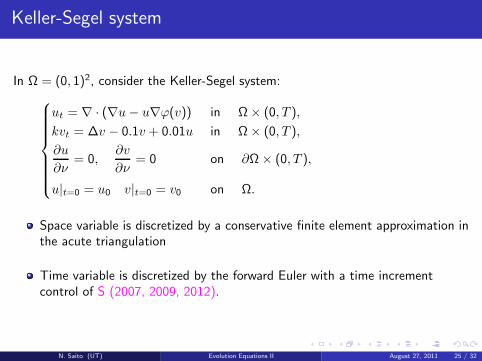
Keller-Segel system

In Ω = (0, 1)2, consider the Keller-Segel system:

ut = ∇ · (∇u − u∇ϕ(v)) in Ω × (0, T ),

kvt = ∆v − 0.1v + 0.01u in Ω × (0, T ),

∂u

∂ν= 0,

∂v

∂ν= 0 on ∂Ω × (0, T ),

u|t=0 = u0 v|t=0 = v0 on Ω.

Space variable is discretized by a conservative finite element approximation inthe acute triangulation

Time variable is discretized by the forward Euler with a time incrementcontrol of S (2007, 2009, 2012).


Keller-Segel system

unh =

unh

‖unh‖∞

の等高線

φ(v) = 5v(1) k = 0.1 (T = 0.19)b0214-43u.wmv; b0214-43v.wmv(2) k = 0.001 (T = 0.14)b0214-46u.wmv; b0214-46v.wmv

φ(v) = 20 log v(3) k = 0.1 (T = 0.21)b0214-57u.wmv; b0214-57v.wmv(4) k = 0.001 (T = 0.27)b0214-58u.wmv; b0214-58v.wmv

φ(v) = 5v2

(5) k = 0.1 (T = 0.011)b0214-63u.wmv; b0214-63v.wmv(6) k = 0.001 (T = 0.002)b0214-66u.wmv; b0214-66v.wmv

***u.wmvが uh

***v.wmvが vh

‖u0h‖1 = 50.0

Windows Media Player で再生して下さい．Macの方は，Flip 4 Macなどをインストールして下さい．


Degenerate Keller-Segel system

In a bounded domain Ω, consider a degenerate Keller-Segel system:

ut = ∇ ·(

∇um − k0u∇vl)

in Ω × (0, T ),

0 = ∆v − v + u in Ω × (0, T ),

∂

∂νum − k0u

∂

∂νvl = 0,

∂v

∂ν= 0 on ∂Ω × (0, T ),

u|t=0 = u0 on Ω.

Space variable is discretized by the cell-centered finite volume approximationin the admissible mesh.

Time variable is discretized by the forward Euler with a time incrementcontrol of S (2007, 2009, 2012).


Numerical example (A): Ω = (0, 1)2

Webブラウザー (Internet Explorer, Netscape, Safariなど)で開いて下さい．m ‖u0‖L1

d0209-1.html 1.0 20.0d0209-2.html 1.2 20.0d0209-3.html 1.4 20.0

Ω = (0, 1)2 square

f(u) = um, g(v) = k0v

k1 = k2 = 1.0, k0 = 5.0

‖u0h‖L1 = 20 > 4π > 2π

If m = 1, the boundary/cornerblow up may occur.

0

0.2

0.4

0.6

0.8

1 0 0.2

0.4 0.6

0.8 1

0

0.2

0.4

0.6

0.8

1

u0h

left figure right figure

unh un

h/‖unh‖L∞


Numerical example (A’): Ω = (0, 1)2

md0209-1x.html 1.0d0209-2x.html 2.0d0209-3x.html 3.0

Ω = (0, 1)2 square

f(u) = um, g(v) = k0v

k1 = k2 = 1.0, k0 = 5.0

x=a; ‖u0‖L1 = 1.0

x=b; ‖u0‖L1 = 5.0

x=c; ‖u0‖L1 = 10.0

x=d; ‖u0‖L1 = 20.0

0

0.2

0.4

0.6

0.8

1 0 0.2

0.4 0.6

0.8 1

0

0.2

0.4

0.6

0.8

1

u0h


unh un

h/‖unh‖L∞


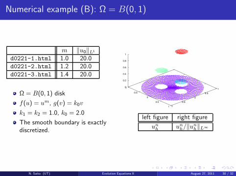
Numerical example (B): Ω = B(0, 1)

m ‖u0‖L1

d0221-1.html 1.0 20.0d0221-2.html 1.2 20.0d0221-3.html 1.4 20.0

Ω = B(0, 1) disk

f(u) = um, g(v) = k0v

k1 = k2 = 1.0, k0 = 2.0

The smooth boundary is exactlydiscretized.

-1

-0.5

0

0.5

1 -1

-0.5

0

0.5

1 0

0.2

0.4

0.6

0.8

1


unh un

h/‖unh‖L∞


Numerical example (C): Ω = B(0, 1)

m l ‖u0‖L1

d0225-6 8.html 1.0 1.0 80.0d0225-6 8.html 1.0 2.0 80.0d0301-6 8.html 1.2 1.0 80.0d0301-6 8.html 1.2 2.0 80.0

Ω = B(0, 1) disk

f(u) = um, g(v) = k0vl

k1 = k2 = 1.0, k0 = 1.0

The smooth boundary is exactlydiscretized.

-1

-0.5

0

0.5

1 -1

-0.5

0

0.5

1 0

0.2

0.4

0.6

0.8

1


unh un

h/‖unh‖L∞


Thank you for your attention!

Norikazu SAITO

Graduate School of Mathematical Sciences

The University of Tokyo

[email protected]

http://www.infsup.jp/saito/


Documents

発展方程式の数値解析 II. Keller-Segel の走化性モデ …発展方程式の数値解析 II. Keller-Segelの走化性モデルと有限体積法 齊藤宣一(Norikazu SAITO)

発展方程式の数値解析 II. Keller-Segel の走化性モデ …発展方程式の数値解析 II. Keller-Segelの走化性モデルと有限体積法齊藤宣一(Norikazu SAITO)