1

Causes of the decline of economic growth in Italy and the responsibility of EURO.

A balance-of-payments approach.

Elias Soukiazisa, Pedro André Cerqueira

a and Micaela Antunes

b

aFaculty of Economics University of Coimbra, and GEMF, Portugal

b Department of Economics, Business and Industrial Engineering, University of Aveiro

and GEMF, Portugal

Abstract

Some countries of the Euro-zone have experienced a declining economic growth more

pronounced in the last recent years, like Italy. The aim of this paper is to investigate the

causes of the poor growth performance in Italy and the responsibility of the Euro for

this crisis. The theoretical approach applied is based on the balance-of-payments

constraint hypothesis (known as Thirlwall’s Law) adapted to include internal and

external imbalances. Our empirical analysis shows that both the extended model and the

original Thirlwall’s Law over-predict the actual growth in Italy suggesting that there are

supply constraints that encumber the economy from growing faster. Another conclusion

is that part of the decline in economic growth is explained by the loss of competiveness

during the Euro period. A scenarios analysis shows that a budget deficit and public debt

discipline aiming at achieving the goals of the Stability Pact are not significant stimulus

for faster growth. On the other hand, reducing the import dependence of the components

of demand, or reducing the import and increasing the export shares in the economy are

the most effective policies for fostering growth in Italy.

JEL code: C32, E12, H6, O4

Keywords: internal and external imbalances, import elasticities of the components of

demand, equilibrium growth rates, 3SLS system regressions.

Author for correspondence: Elias Soukiazis, Faculty of Economics, University of Coimbra,

Av. Dias da Silva, 165, 3004-512 Coimbra, Portugal, Tel: +351239790534, Fax:

+351239790514, e-mail: elias@fe.uc.pt

2

1. Introduction

Thirlwall (1979) developed a simple model that determines the long-run rate of growth

of an economy consistent with the balance-of-payments equilibrium. According to this

rule, actual growth can be predicted by the ratio of export growth to the income

elasticity of demand for imports and this simple relation became known as Thirlwall’s

Law. The Law advocates that no country can grow faster than its balance-of-payments

equilibrium growth rate, unless it can continuously finance external deficits by capital

inflows. Growth is constrained by external demand, and balance-of-payments

disequilibrium on the current account can be a serious obstacle to faster growth when it

cannot be financed by available foreign resources. A crucial implication of the model is

that it is income and not relative prices that adjust to bring the economy back to

equilibrium.

Thirlwall and Hussain (1982) revised the initial model relaxing the assumption that the

balance-of-payments is initially in equilibrium. Since countries can run current account

deficits, capital inflows can be included in the model to determine the long-term growth

rate. This model has shown to be more suitable especially for developing countries

where external imbalances can be sustained by capital inflows that alleviate the pressure

on external payments. A large number of empirical studies emerged testing the validity

of Thirlwall’s Law or criticising the basic assumptions that it relies on. Among others,

Moreno-Brid (1998-99), McCombie and Thirlwall (1994) and recently Blecker (2009)

have made valuable contributions discussing and criticising the underlying implications

of the Law.

The hypothesis of constant relative prices has been criticised widely in empirical

literature (see for example, McGregor and Swales, 1985; 1991; Alonso and

Garcimartín, 1998-99; López and Cruz, 2000). But in most studies in this field, relative

prices have been shown to be statistically insignificant and even when they are

significant the price elasticities with respect to imports and exports are very low in

magnitude when compared to the income elasticities, showing that imports and exports

are less sensitive to price changes than to income changes. Alonso and Garcimartín

(1998-99) showed that the assumption that prices do not matter in determining the

equilibrium income is neither a necessary nor a sufficient condition to affirm that

growth is constrained by the balance-of-payments. The empirical evidence seems to

3

support that income is the variable that adjusts to bring into equilibrium the external

imbalances, implying therefore that growth is indeed balance-of-payments constrained.

Blecker (2009) also stressed that it is reasonable to conclude that the longer the time

period considered, the more likely it is that relative prices remain constant. On the other

hand, increasing capital inflows can at most be a temporary way of relaxing the balance-

of-payments constraint, but they do not allow a country to grow at the export-led

cumulative growth rate in the long-term. What matters in the long-term analysis of

growth is the growth of exports.

On the sustainable debt debate, Barbosa-Filho (2002) argued that since the home

country does not issue foreign currency, it can only have persistent trade deficits by

receiving a continuous inflow of foreign capital. The counterpart of unbalanced trade is

a change in the stock of foreign debt and, therefore, it has to be checked under which

conditions the unbalanced trade constraint is consistent with a non-explosive

accumulation of foreign debt.

Although Thirlwall’s model has been modified to include capital flows and foreign

debt, these studies have not considered the role of public imbalances as an additional

constraint on growth. The external imbalance considered so far in the literature includes

public disequilibrium, but the impact of the latter on overall growth has not been

analysed separately. The recent experience of some peripheral European countries

falling into public debt crisis is the motivation to deal with this issue. As Pelagidis and

Desli (2004) argue, the implementation of an expansionary fiscal policy, aiming at

strengthening growth rates and reducing unemployment, would not always achieve the

desirable objectives. It could be the case that budget deficits, financed either by money

printing or by public borrowing, will increase public debt and interest rates, crowd out

private investments, fuel inflation, and damage medium-term growth. The answer to

whether budget deficits are always desirable has many dimensions, including whether

government borrowing is financing government consumption or investment in

infrastructure, whether the deficit is sustainable, and how it is financed. On the other

hand, the hesitation of many policy makers – especially in Europe – to rely more

aggressively on fiscal policy measures in order to keep their public finances more or

less balanced may lead to the possibility of a vicious cycle between slow growth and

higher deficit formation as a result of the reduction of tax revenues.

4

Our paper aims at contributing to this debate by performing an alternative growth

model, in line with Thirlwall’s Law, that takes into account not only external, but also

internal imbalances due to budget deficits and public debt. The reduced form of the

growth of domestic income is determined, among others, by factors related to

competitiveness and mismanagement of fiscal policy and public finances that could

affect economic growth negatively. The theoretical model is tested for the Italian

economy that recently faced serious problems in financing its public debt in

international financial markets. The implemented restrictive measures, monitored by the

IMF, are expected to have negative repercussions on growth in the upcoming years.

Another issue to address is whether the adoption of Euro is responsible for the decline

in economic performance in Italy. Taking all these considerations into account, the

paper is organized as follows: in section 2 we present the theoretical growth model;

section 3 tests the model for the Italian economy, for the whole period and the pre and

post Euro sub-periods, trying to understand the causes of economic growth. The last

section concludes.

2. The growth model with internal and external imbalances

We use a multi equation model developed by Soukiazis-Cerqueira-Antunes (2012) -

hereafter the SCA model - to derive the reduced form of income growth which depends,

among other things, on internal and external imbalances. The model follows the

developments of Thirlwall’s Law with two particular differences: (i) it considers not

only external imbalances (current account deficits) but also internal imbalances

emerging from public deficit and debt; (ii) it considers further the import contents of the

components of aggregate demand, measuring their impact on growth.

The SCA model is constituted by the following main equations, where a lower-case

letter with a dot denotes the instantaneous growth rate of a given variable:

(i) Import equation

Contrary to the conventional specification that considers real domestic income as the

main aggregate determinant of the demand for imports, we use the components of

domestic income to explain import flows. We assume that relative prices do not play a

5

significant role and that in the long-run they remain constant (the steady state

condition)1. The import function is given by:

kxgcm kxgc&&&&& ππππ +++= (1)

where the growth in demand for imports ( m& ) depends on the growth rates of private

consumption ( c& ), government expenditures ( g& ), exports ( x& ) and investment ( k& ),

respectively. In this equation, π stands for the elasticity of each of the components of

demand in relation to imports. All elasticities are expected to be positive since all

components of demand have import content.

(ii) Government expenditure

As it is shown in the SCA model (see Appendix II of the mentioned paper), the long-

term relationship of the growth of real government expenditures is given by:

G

B

G

B

G

D

G w

wpi

w

wbip

w

wd

w

ytg &&&&

&& ++−+= )( (2)

where Y

PDwD

/= is the public deficit ratio,

D

Dd

∆=& the growth rate of public deficit,

Y

GwG = denotes the public expenditure share and

Y

PBwB

/= the public debt share.

Equation (2) is derived from the government budget relation given by the following

identity:

DYPtiBGn +=+ )(

where Gn is nominal government expenditures, B is public debt 2

, Y is domestic income,

P is the domestic price level, D the public deficit, i is nominal interest rate paid on

public debt and t is the tax rate on nominal income. According to this relation, public

1 This is a debatable assumption made for the sake of simplifying the model. As we explained before,

there are studies showing that relative prices are important in international trade and explain a

substantial part of growth in some countries. For instance, Garcimartín et al (2010-11) attribute the

slowdown of economic growth in Portugal to the overvaluation of the domestic currency (loss of price

competitiveness) when the country joined the Euro zone.

2 Public debt is originated by the issue of government bonds to finance public deficit.

6

deficit exists when total current expenditures (including interest payments on public

debt) exceed the receipts obtained through taxes on domestic money income,

Gn+iB>t(YP).

We have to note that the public debt (B) is a combination of both domestic (BH) and

foreign (BF) debt, that is, government’s bonds are held by residents and non-residents,

respectively. Likewise, the public deficit (D) can be financed internally (DH) or from

abroad (DF). Bearing this in mind, the following relations are established:

D

D

D

D

D

D

D

DDDD

B

B

B

B

B

B

B

BBBB

F

D

H

D

FH

FH

F

B

H

B

FH

FH

=−==++=

=−==++=

ξξ

ξξ

1;;1;

1;;1;

(3)

whereBξ (the percentage of public debt financed internally) and

Dξ (the percentage of

public deficit financed internally) are assumed to be constant in the long-run, for

simplicity. The extreme case Bξ =1 shows that public debt is uniquely financed by

national bond holders. Analogously,Dξ =1 implies that the budget deficit is entirely

financed by domestic resources.

(iii) Private final consumption and investment

From the SCA model (see Appendix III of the mentioned paper) the growth of

consumption ( c& ) is a function of the growth of domestic income ( y& ) with cε the income

elasticity with respect to consumption:

yc c&& ε= (4)

Analogously, the growth of investment is a function of the growth of domestic income (

y& ) with kε the income elasticity in relation to change in capital stock:

yk k&& ε= (5)

(iv) Export demand function

In this equation it is assumed that foreign income Y* is the main determinant of export

demand. It is explicitly assumed that exports competitiveness is based on non-price

7

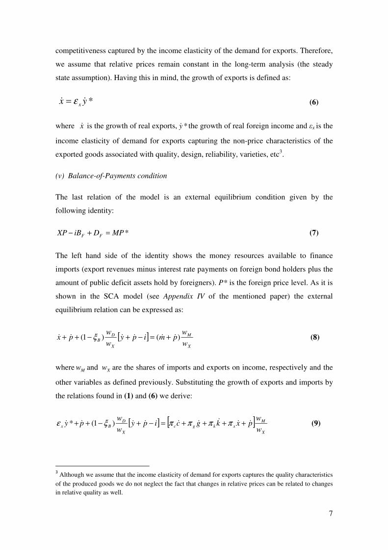
competitiveness captured by the income elasticity of the demand for exports. Therefore,

we assume that relative prices remain constant in the long-term analysis (the steady

state assumption). Having this in mind, the growth of exports is defined as:

*yx x&& ε= (6)

where x& is the growth of real exports, *y& the growth of real foreign income and εx is the

income elasticity of demand for exports capturing the non-price characteristics of the

exported goods associated with quality, design, reliability, varieties, etc3.

(v) Balance-of-Payments condition

The last relation of the model is an external equilibrium condition given by the

following identity:

*MPDiBXP FF =+− (7)

The left hand side of the identity shows the money resources available to finance

imports (export revenues minus interest rate payments on foreign bond holders plus the

amount of public deficit assets hold by foreigners). P* is the foreign price level. As it is

shown in the SCA model (see Appendix IV of the mentioned paper) the external

equilibrium relation can be expressed as:

[ ]X

M

X

D

Bw

wpmipy

w

wpx )()1( &&&&&& +=−+−++ ξ (8)

where Mw and Xw are the shares of imports and exports on income, respectively and the

other variables as defined previously. Substituting the growth of exports and imports by

the relations found in (1) and (6) we derive:

[ ] [ ]X

M

xkgc

X

D

Bxw

wpxkgcipy

w

wpy &&&&&&&&& ++++=−+−++ ππππξε )1(* (9)

3 Although we assume that the income elasticity of demand for exports captures the quality characteristics

of the produced goods we do not neglect the fact that changes in relative prices can be related to changes

in relative quality as well.

8

Further substitution of the growth of government expenditure (2), consumption (4),

investment (5) and exports (6) yields:

[ ]

X

M

G

B

G

B

G

D

G

gxxkkcc

X

D

Bx

w

wp

w

wpi

w

wbip

w

wd

w

ytyyy

ipyw

wpy

+

++−++++

=−+−++

&&&&&&

&&&

&&&&

)(*

)1(*

πεπεπεπ

ξε

(10)

The next step is to define domestic income growth and find its determinants.

(vi) Domestic income growth

Rearranging terms in equation (10) we derive the reduced form of the growth of

domestic income as it is shown in the SCA model (see Appendix V of the mentioned

paper):

M

D

B

G

B

G

D

G

gkkcc

G

B

G

D

g

M

D

B

M

X

xx

M

X

x

w

w

w

wip

w

w

w

t

pw

wp

w

wp

w

rwp

w

wy

w

w

y

)1())((

)1(*)( 2

ξπεπεπ

πξεπε

−−+−+++

−

−−−−+−

=

&

&&&&&

& (11)

Equation (11) shows that among other factors the growth of domestic income is

determined by internal and external imbalances. Furthermore if we assume internal and

external equilibrium (B=0, D=0 and X=M), Equation (11) reduces to4:

gkkcc

xxx yy

πεπεπ

επε

++

−=

*)( && (12)

Equation (12) is similar to Thirlwall’s original Law given by

π

ε *yy x

&& = (13)

The only difference is that Equation (12) takes into account the import content of

exports in the numerator and the import content of other components of domestic

demand in the denominator. It would be interesting to test empirically these alternative

4 We are assuming that prices, real interest rates, the deficit and debt ratios are constant in the long-run.

Also, t/wG=1.

9

versions and check the difference in the prediction of domestic growth both in the

presence and in the absence of internal and external imbalances.

3. Testing the model for the Italian economy

Econometric Methodology

The import Equation (1), consumption Equation (4), investment Equation (5) and export

Equation (6) are all estimated simultaneously to obtain the elasticities which are needed

to compute the reduced form of domestic income growth as it is expressed in Equation

(11). The definition of the variables and the data sources are explained in Appendix A at

the end of the paper. The method used for estimating the system equations is 3SLS

(Three-Stage Least Squares) as it is more efficient to capture the interrelation between

equations and the causal and feedback effects between the variables.5 Table B.1 in the

Appendix B provides the regression results where simultaneity is controlled by using

instrumental variables. The growth of imports, consumption, investment and exports are

assumed to be endogenous as well as the growth of government expenditures and

domestic income. All other variables of the system are assumed exogenous including

some lagged variables, as it is explained in Table B.1.

We also regressed each of the equations individually, by 2SLS (Two-Stage Least

Squares), with the same instruments as before. The intention was to carry out some

diagnostic tests to justify the robustness of our results. The first is the Sargan statistic, a

test of over-identifying restrictions to check the validity of the instruments used in the

regressions and that hypothesis is confirmed in all cases. The second is the Pagan-Hall

heteroscedasticity test, showing that the hypothesis of homoscedasticity is never

rejected. The third test is the Cumby-Huizinga test for autocorrelation. The null

hypothesis, which is not rejected at 5% significant level in all cases, is that errors are

not first-order autocorrelated. The last one is a normality test, conceptually similar to

the Jarque-Bera skewness and kurtosis test. The null hypothesis is that residuals from a

given regression are normally distributed, and this hypothesis is not rejected in all

equations (except for investment). The results are displayed on Table B.2. in Appendix

B.

5 For more details on the 3SLS method, see for instance, AlDakhil (1998) and Wooldridge (2002).

10

Empirical results and discussion

Table 1 below reports the values which are necessary for computing the growth of

domestic income in Italy. Some are estimated values taken from Table B.1 (Appendix

B) others are annual averages over the periods considered (see Appendix A for variable

definition and data sources).

Three different growth rates are computed and presented at the bottom of the table: ay&

obtained from Equation (11) where internal and external imbalances are considered; by&

obtained from Equation (12) where internal and external equilibrium is assumed, and cy&

obtained from Thirlwall’s Law, given byπ

ε *yy x

&& = (see Equation (13)). In the latter

case, it was necessary to estimate the import demand function, yam m&& π+= , by OLS

to obtain the aggregate income elasticity with respect to import growth6. Additionally,

we provide values of the actual growth in the whole period (1984-2010), the pre-Euro

period (1984-1998) and the post-Euro period (1999-2010). We assume that the

estimated parameters of the model for the whole period are the same in the two sub-

periods since the time span is too short to allow us to implement separate regressions of

the system. The variables of the model assume their average values in the respective

periods. The aim is to investigate whether there are differences in growth rates between

the two sub-periods thus identifying different sources of economic growth.

Analysing the results of the computation of the growth rates for Italy shown in Table 1,

we can make the following remarks:

(i) The growth rates obtained from Thirlwall’s Law ( cy& ), given by π

ε *yy x

&& =

overestimate the actual growth achieved in Italy in all periods, cy& > y& , and this should

be consistent with the existence of trade surpluses or at least with a balanced trade. If

we check the figures of the share of exports ( Xw ) and imports

6 The import equation was also estimated with relative prices as additional explanatory variable, but its

coefficient was not significant and there was no significant change of the income elasticity.

11

Table 1. Computation of the growth rates of domestic income in Italy.

1984-2010 xε

2.6

2.6

2.6

xπ

0.506

0.506

0.506

cε

0.800

0.800

0.800

cπ

0.849

0.849

0.849

kε

2.127

2.127

2.127

kπ

0.402

0.402

0.402

gπ

0.083

0.083

0.083

r

0.039

0.054

0.022

t

0.427

0.418

0.448

1984-1998

1999-2010

1984-2010 Dw

0.069

0.095

0.031

Gw

0.423

0.419

0.432

Bw

1.019

1.015

1.084

Dξ

0.58

0.58

0.58

Bξ

0.58

0.58

0.58

Mw

0.226

0.198

0.262

Xw

0.234

0.213

0.264

p&

0.052

0.059

0.023

*y& MX ww /

0.026 1.035

0.032 1.076

0.021 1.008

1984-1998

1999-2010

1984-2010 ay& =2.205%

ay& =2.868%

ay& =1.656%

Internal and

external

imbalances

Equation (11)

by& =2.053%

by& =2.505%

by& =1.629%

Internal and

external

equilíbrium

Equation(12)

cy& =2.375%

cy& =2.50%

cy& =2.011%

Thirlwall’s

Lawa

Equation (13)

y& =1.504%

y& =2.173%

y& =0.667%

Actual

growth

1984-1998

1999-2010

Notes:

xε , xπ , cε , cπ , kε , kπ and gπ are taken from Table B.1 (Appendix B).

r, t, Dw , Gw , Bw , Mw , Xw , Dξ ,

Bξ , p& and *y& are annual averages over the periods 1984-2010, 1984-1998 and 1999-2010, respectively.

a The import equation ( yam m

&& π+= ) was estimated by OLS to derive the aggregate income elasticity of demand for imports mπ which is 2.846 for the whole period 1984-

2010, 3.325 for the pre-euro period 1984-1998, and 2.715 for the post-euro period 1999-2010.

12

( Mw ) they are similar, showing that Italy is close to a balanced economy with

respect to external trade7. In particular, the ratio of the share ( MX ww / ) is greater

than one in all periods (see Table 1), although it has decreased moderately in the

post-euro period. Two main conclusions can be derived from these results. The

first is that Thirlwall’s Law - through Equation (13) - overpredicts actual growth

in Italy, showing that the country has the potentiality to grow faster than actually

did. The second is that Italy slightly loses competitiveness in the post-euro

period and this can be part of the explanation for the anemic economic growth

observed in the last decade.

(ii) The growth rates computed by the SCA model - Equation (12) - when internal and

external equilibrium is assumed ( by& ), also overestimate the actual growth in Italy in all

periods and lead to the same conclusions as Equation (13). On the other hand, the

predicted growth rates from the SCA model are closer to the actual rates in Italy than

those obtained from Thirlwall’s Law. Our estimates indicate that Italy has grown slower

than the rate allowed by the balance-of-payments equilibrium ( byy && < < cy& ) and this

can be taken as evidence that this country faces supply constraints, restraining the

economy from growing faster8. In other words Italy’s potential growth

9 (without

harming the balance-of-payments position) is higher than that actually achieved and the

explanation for this slower growth rate can be found on the existence of supply

constraints10

. As it is known, once the economy becomes supply-constrained, demand

growth has no effects on the rate of output growth. Two main remarks can be made

from this analysis. The first is that the SCA model –Equation (12) – that takes into

account the disaggregate demand elasticities of imports ),,( gxkc and ππππ is more

accurate for predicting actual growth in Italy than the original Thirlwall’s Law –

through Equation (13) – that considers the aggregate income elasticity of the demand

7 The current account as a percentage of GDP in Italy was on average positive 0.249% in the period 1984-

1998 but negative -1.04% in the euro period. The last result was greatly influenced by the recession years

of 2008 and 2009. Anyway, these figures are not very far for assuming that the external trade is close to

equilibrium. 8 Some previous studies obtained the same result for Italy, for instance Thirlwall (1979; 1982) for the

period 1953-1976, McCombie (1985) for 1973-1980, Pattichis (2001) for 1960-1997, and Bagnai (2008)

for 1960-2006. 9 The definition of potential growth is different than that implying full capacity utilization of factors of

production. In this text we mean the growth achieved without creating balance-of-payments deficits. 10

The supply restrictions can rely on the lack of production organization, low productivity, labour market

rigidities, financial constraints, high bureaucracy, inefficient legislation, state interference, among others.

For instance, total factor productivity growth in Italy is declining over time with the average value being

1.7% in 1986-1990, 1.2% in 1991-1995, 0.8% in 1996-2000, 0.3% in 2001-2005, and -0.5% in 2006-

2010.

13

for imports )(π . The second is that there is evidence that Italy is subject to supply

constraints that obstruct the country from growing faster.

(iii) The growth rates computed by the SCA model – through Equation (11) that takes into

account the internal and external imbalances - give the same insights as the previous

case. In fact the predicted growth rates are higher than the actual rates achieved in Italy

for all periods indicating again that the country is under supply constraints. These

computed growth rates are also slightly higher than the rates obtained from Equation

(12) where internal and external equilibrium is assumed. Therefore, the SCA model -

with or without (internal and external) equilibrium – and Thirwall´s Law all agree that

Italy has the potentiality to grow faster (without creating balance-of-payments

problems), whenever the supply constraints are removed.

(iv) When we divide the whole period in the pre-euro and the post-euro periods we

observe that Italy grew much slower in the latter than in the former (0.667%11

versus 2.173%). How can we justify this disappointing result for the country’s

economic performance? Is our model able to explain this radical decline in

growth? The answer is yes. We have already mentioned above two causes for

the decline in economic growth in Italy in the era of the euro: the first has to do

with the loss of competiveness shown by the decline in the export/import share

ratio, from 1.076 to 1.008 (see Table 1) and the deterioration of the current

account equilibrium, from a 0.249% average surplus before the euro period to -

1.04% deficit in the euro period (see footnote 7). The second is that Italy has the

potentiality to grow faster without harming the balance-of-payments

equilibrium, but this did not happen because of supply constraints which are

more pronounced in the post-euro period. We can clarify this idea by checking

the difference between actual growth and that predicted by the SCA model

which is higher in the post-euro period (1.656-0.667=0.989) than in the pre-euro

period (2.868-2.173=0.695).

Some other causes that could explain the lower growth rates in the euro period,

as Table 1 shows, can be found on the increasing rate of taxation (from 41.8% to

44.8% on average), the increase in the public debt (from 101.5% of GDP to

11

We have to take into account that the average slower growth rate in the euro period is heavily

influenced by the negative decline of GDP by -1.2% in 2008 and -5.1% in 2009.

14

108.4% on average), the increase in public expenditure share12

(from 41.9% to

43.2% on average) but also on exogenous factors as the decline of external

growth (from 3.2% to 2.1% on average).

Summing up, we believe that there are three main directions that Italy should

focus in order to recover economic growth: removing the supply constraints to

growth (improvements in productivity); increasing external trade

competitiveness; and adjusting public imbalances to more suitable levels.

Scenarios to faster growth

Some scenarios can be designed to try to detect some policies that could help Italy to

grow faster, using the SCA model with internal and external imbalances – Equation (11)

- for the global period.

(i) First of all we can find the impact on growth by imposing a public deficit of wD

=3% and a debt discipline of wB = 60% (as percentages of GDP), which are the

goals of the Stability and Growth Pact in Europe. Imposing these goals in the

SCA model the predicted growth rate for Italy increases from ay& =2.205% (see

Table 1) to 2.289% which is not a significant improvement. Although the fiscal

policy discipline helps Italy to improve its growth performance in the long-term,

this measure is not a great stimulus to growth.

(ii) Reducing the import sensitivity of exports (elasticity) from xπ =0.506 to 0.40

our model predicts a rise in the growth rate from ay& =2.205% to ay& = 2.69% and

if xπ = 0.30 the growth rate is even higher, ay& = 3.15%. Having a large import

sensitivity of exports is an impediment to growth since the exports’ multiplier

effects on income are crowded out by higher imports. Reducing the import

content of exports is the appropriate policy to achieve higher growth in Italy. We

have to notice however, that living in a global economy where production is

organized around international value chains, what is important is not importing

too much in order to produce exports, but ensuring that the transformation of

imported components into exports contains enough value-added. In international

12

If public spending removes resources from private investment, a large public sector is likely to act as a

constraint on growth.

15

markets, most exports embody a substantial share of imported components, but

in terms of gains it is important that the value (price) of exports embodying

imported components is sufficiently higher than the value (price) of those

imported components.

(iii) Growth rates in Italy are also sensitive to import contents of other components of

demand like consumption and investment. Reducing the import sensitivity of

consumption from cπ =0.849 to 0.70 and that of investment from kπ =0.402 to

0.30 the predicted growth rate obtained from the SCA model increases from ay&

=2.205% to ay& =2.86% which is a significant improvement. Assuming a more

pronounced reduction cπ =0.65 and kπ =0.25 the growth rate increases to ay&

=3.28% Therefore, policies regarding a drop in the import dependence of the

elements of demand can be a good strategy for fostering economic growth in

Italy.

(iv) Increasing the share of exports by two percentage points (from 23% to 25%) the

obtained growth is ay& = 2.77%, or alternatively reducing the share of imports by

only two percentage points (from 22%% to 20%) the predicted growth is even

faster, of about ay& = 3.28%. A combined policy with the aim at reducing the

import share to 20% and increase the export share to 25% (with a surplus on

trade) yields an even faster growth rate, around ay& = 3.91%. Therefore changing

the structure of the shares of imports and exports is the appropriate way to

achieve higher growth in Italy.

These hypothetical scenarios clearly show that the most effective policy to achieve

faster growth in Italy is related to the external sector, either through an effort to obtain a

positive net trade or to lower the import content of the components of demand. This is in

line with the balance-of-payments equilibrium approach supported by Thirlwall’s Law.

4. Concluding remarks

The aim of this study was to apply an alternative growth model in line with Thirlwall’s

Law that takes into account both internal and external imbalances. The important

contribution of the model is that it discriminates the import content of aggregate

16

demand and introduces public deficit and debt measures as determinants of growth. The

reduced form of the model shows that growth rates can be obtained in three alternative

ways: (i) assuming internal and external imbalances (the so called SCA model); (ii)

assuming that public finances and current account external payments are balanced; and

lastly (iii) the growth rate predicted by Thirlwall’s Law. The SCA growth model is

tested for the Italian economy to check its accuracy.

The equations constituting the SCA model are estimated by 3SLS to control the

endogeneity of variables and to obtain consistent estimates. Growth rates are estimated

for the whole period 1984-2010 and also for the pre and post euro periods. The

empirical analysis shows that growth rates obtained by the SCA model and the

Thirlwall’s Law over-predict actual growth in Italy in all periods considered, providing

evidence that Italy grew slower than the rate compatible with the balance-of-payments

equilibrium hypothesis. According to the interpretation of this hypothesis, the causes for

the slower economic performance can be found on supply constraints that obstruct the

economy from growing faster. Another important finding is that Italy’s economic

growth is much slower in the euro period and the main explanation may lay in the loss

of competitiveness in this period. Other factors that possibly contributed to the decline

of growth are higher public deficits and debt, higher taxes and high public expenditure.

Some scenarios are implemented to detect policies that could foster economic growth in

Italy. It is shown that imposing the Stability and Growth Pact measures related to fiscal

discipline (3% budget deficit and 60% public debt as percentages of GDP) are not

significant stimulus for higher growth. Policies aiming at reducing the import contents

of the components of demand or reducing by only two percentage points the import

share and increasing by the same amount the export share in the economy are the most

effective policies to promote economic growth in Italy.

17

Appendix A

Description of the variables and data sources

• tm& – annual growth rate of real imports - Imports of goods and services at 2000 prices

(national currency; annual percentage change).

• tc& – annual growth rate of final private consumption - Private final consumption

expenditure at 2000 prices (national currency; annual percentage change).

• tx& – annual growth rate of real exports - Exports of goods and services at 2000 prices

(national currency; annual percentage change).

• – annual growth rate of investment - Gross fixed capital formation at 2000 prices

(national currency; annual percentage change).

• ty& – annual growth rate of real GDP - GDP at 2000 market prices (national currency; annual

percentage change).

• tp& – annual growth rate of price deflator GDP at market prices (national currency; annual

percentage change).

• wG – share of government’s expenditure on GDP - Total expenditure; general government

(% of GDP at market prices; excessive deficit procedure).

• wD – share of government’s deficit on GDP - Net lending (-) or net borrowing (+); general

government (% of GDP at market prices; excessive deficit procedure).

• wB – share of government’s debt on GDP - General government consolidated gross debt (%

of GDP at market prices; excessive deficit procedure). It excludes interest rate payments on

debt.

• wM - imports of goods and services at current prices (national accounts) - % of GDP at

market prices

• wX-. exports of goods and services at current prices (national accounts) - % of GDP at

market prices.

• t – share of government’s revenues on GDP - Total current revenue; general government (%

of GDP at market prices; excessive deficit procedure).

• i – nominal long-term interest rates (%)

Data on tm& , tc& , tx& , , ty& , tp& , wG, wD, wB,,wM, wX, t and i were taken from European

Commission (2011).

• tg& – annual growth rate of government’s expenditure. Computed by the authors from

data on general government expenditure (Millions of euro from 1.1.1999/ECU up to

31.12.1998), available on Eurostat - Government Accounts

http://epp.eurostat.ec.europa.eu/portal/page/portal/statistics/search_database (extracted on 12th

December, 2011) and information ontp& .

• *y& - annual growth rate of real foreign income (OECD countries), excluding Italy. The

rates were computed by the authors, using data obtained from OECD.StatExtracts

http://stats.oecd.org/Index.aspx (extracted on 15th December, 2011).

tk&

tk&

18

Appendix B

Table B.1. The 3SLS estimation of the structural model, Italy 1984-2010.

Coefficient Std Error t-stat p-value R2 F-stat p-value

Imports growth

constant

0.156 0.849 0.18 0.854

0.8048 26.04 0.000 0.849 0.485 1.75 0.083*

0.083 0.115 0.72 0.471

0.506 0.112 4.50 0.000***

0.402 0.188 2.14 0.035**

Consumption growth

constant

0.405 0.281 1.44 0.154 0.5904 46.72 0.000 0.800 0.117 6.84 0.000***

Investment growth

constant

-1.636 0.566 -2.89 0.005*** 0.7430 78.07 0.000 2.127 0.241 8.84 0.000***

Exports growth

constant

-3.429 1.378 -2.49 0.015** 0.5870 35.89 0.000 2.600 0.434 5.99 0.000***

Notes:

Endogenous variables: �� �, ��� , �� � , ��� , �� �, ��

Exogenous variables: ��∗ � ��

∗ ��,� ��,��� ��,� ��,��� ��,� ��,��� �� �� �� ,� �� .�� �� .��� �� ���

�� ��� �� ��� �� ���

* Coefficient significant at the 10% level; ** Coefficient significant at the 5% level; *** Coefficient

significant at the 1% level.

tk&

tc&

tg&

tx&

ty&

ty&

*ty&

19

Table B.2. The 2SLS estimation of each equation of the structural model, Italy 1984-2010.

Coefficient

Std

Error t-stat p-value

Sargan

test

Heteroscedasticity

test AR(1) test Normality test

Growth of imports

constant

0.395 0.971 0.41 0.688 χ213=18.058 χ

217=11.599 χ

21=1.854 χ

22=0.43

1.025 0.576 1.78 0.089* p-value=0.1553 p-value=0.8238 p-value=0.1733 p-value=0.8050

0.017 0.137 0.12 0.904

0.405 0.133 3.06 0.006***

0.518 0.224 2.32 0.030**

Growth of consumption

constant

0.522 0.298 1.75 0.093* χ216=22.742 χ

217=19.266 χ

21=0.6657 χ

22=2.59

0.722 0.128 5.64 0.000*** p-value=0.1208 p-value=0.3135 p-value=0.4145 p-value=0.2738

Growth of investment

constant

-1.507 0.592 -2.54 0.017** χ216=20.881 χ

217=16.481 χ

21=3.2496 χ

22=11.92

2.042 0.254 8.04 0.000*** p-value=0.1831 p-value=0.4901 p-value=0.0714 p-value=0.0026

Growth of exports

constant

-3.868 1.357 -2.85 0.008*** (1)

χ21=0.195

(2) χ

21=1.4415 χ

22=3.61

2.789 0.443 6.30 0.000*** p-value=0.6588 p-value=0.2299 p-value=0.1644

Notes:

Endogenous variables: �� �, ��� , �� � , ��� , �� �, ��. Exogenous variables: ��∗ � ��

∗ ��,� ��,��� ��,� ��,��� ��,� ��,��� �� �� �� ,� �� .�� �� .��� �� ��� �� ��� �� ��� �� ���

* Coefficient significant at the 10% level; ** Coefficient significant at the 5% level; *** Coefficient significant at the 1% level.

(1) The last equation is an OLS regression; there is no Sargan test.

(2) The heteroscedasticity test on the last equation is a White/Koenker NR2 test statistic. The Breusch-Pagan/Godfrey/Cook-Weisberg test points to the same conclusion: χ

21 =

0.189; p-value = 0.6634.

tk&

tc&

tg& tg&

tx& tx&

ty&

ty&

*ty&

20

References

AlDakhil, K. (1998) “ A method for estimating simultaneous equations models with

time-series and cross-section data”. Journal of King Saud University - Administrative

Sciences, 10 (1) 13-28.

Alonso, J., Garcimartín, C., (1998-99) “A new approach to balance-of-payments

constraint: some empirical evidence”. Journal of Post Keynesian Economics. Winter,

21(2), 259-282.

Bagnai, A. (2008) “Structural changes, cointegration and the empirics of Thirlwall´s

Law”. Applied Economics, vol. 37(8), 1-15.

Barbosa-Filho, N., (2002) “The balance-of-payments constraint: from balanced trade to

sustainable debt”. CEPA Working Paper, January.

Blecker, R., (2009) “Long-run growth in open economies: export-led cumulative

causation or a balance-of-payments constraint”? Paper presented at the 2nd

Summer

School on Keynesian Macroeconomics and European Economic Policies. 2nd

-9th

August, Berlin, Germany.

European Commission (2011) “Statistical Annex of European Economy”. Directorate

General Economic and Financial Affairs, Spring.

Garcimartín, C., Rivas, L., Martínez, P. (2010-11) “On the role of relative prices and

capital flows in balance-of-payments constrained growth: the experiences of Portugal

and Spain in the Euro Area”. Journal of Post-Keynesian Economics. Winter, 33 (2),

281-306.

López, J.; Cruz, A. (2000) “Thirlwall’s Law and beyond: the Latin American

experience”. Journal of Post Keynesian Economics. Spring, 22(3), 477-495.

McCombie, J. (1985) “Economic growth, the Harrod foreign trade multiplier and the

Hick’s super-multiplier”. Applied Economics, 17, 55-72.

21

McCombie, J., Thirlwall, A., (1994) “Economic growth and the balance-of-payments

constraint”. MacMillan Press, Basingstoke; St. Martin’s Press, New York.

McGregor, P., Swales, J. (1985) “Professor Thirlwall and the balance-of-payments

constrained growth”. Applied Economics. 17, 17-32.

McGregor, P., Swales, J., (1991) “Thirlwall’s Law and balance-of-payments

constrained growth: further comment on the debate”. Applied Economics. 23, 9-23.

Moreno-Brid, J., (1998-99) “On capital flows and the balance-of-payments-constrained

growth model”. Journal of Post Keynesian Economics. Winter, 21(2), 283-298.

Pattichis, C. (2001) “Trade, growth and monetary union”. Journal of Post Keynesian

Economics. Fall, 24(1), 125-148.

Pelagidis, T., Desli, E. (2004) “Deficits, growth and the current slowdown: what role for

fiscal policy?” Journal of Post Keynesian Economics. Spring, 26 (3), 461-469.

Soukiazis, E., Cerqueira P., Antunes, M. (2012) “Modelling economic growth with

internal and external imbalances: empirical evidence from Portugal”. Economic

Modelling. 29 (2), 478-486.

Thirlwall, A., (1979) “The balance-of-payments constraint as an explanation of

international growth rate differences”. Banca Nazionale del Lavoro. 128, 45-53.

Thirlwall, A., (1982) “The Harrod trade multiplier and the importance of export-led

growth”. Pakistan Journal of Applied Economics. 1(1), 1-21.

Thirlwall, A., Hussain, N., (1982) “The balance-of-payments constraint, capital flows

and growth rate differences between developing countries”. Oxford Economic Papers.

34, 498-510.

Wooldridge, J. (2002) “Econometric analysis of cross-section and panel data”.

Cambridge, Massachusetts, MIT Press.