Causes of Bank Suspensions in the Panic of 1893

Mark Carlson*

Federal Reserve Board

There are two competing theories explaining bank panics. One argues that panics are driven by real shocks, asymmetric information, and concerns about insolvency. The other theory argues that bank runs are self-fulfilling, driven by illiquidity and the beliefs of depositors. This paper tests predictions of these two theories using information uniquely available for the Panic of 1893. The results suggest that real economic shocks were important determinants of the location of panics at the national level, however at the local level, both insolvency and illiquidity were important as triggers of bank panics.

* Federal Reserve Board, Mail Stop 86, 20th and Constitution Ave. NW, Washington DC, 20551. Mark.A.Carlson@frb.gov. I have benefited greatly from conversations with Greg Duffee, Barry Eichengreen, and Christina Romer, as well as comments from Richard Grossman and seminar participants at the University of Virginia. Thank you also to Shaun Boyd for generous assistance collecting information about the experience of Colorado during the crisis. The views presented in this paper are solely those of the author and do not necessarily represent those of the Federal Reserve Board or its staff.

1

The National Banking Era, extending from 1865 until 1913, witnessed five major financial

panics (Sprague 1910). These crises caused hundreds of national banks to suspend operations,

constituting major disruptions of the financial system. In the Panic of 1893, roughly 575 banks

either failed or temporarily suspended operations (Bradstreet’s 1893). Clearinghouses in 73 cities

partially suspended cash payments in the Panic of 1907. During the three most severe crises, those

of 1873, 1893, and 1907, specie was hoarded and circulated at a premium over checks drawn on

banks, even in major financial centers such as Boston and New York City. Due to the disruptions

in the financial system, some non-financial businesses found it difficult to obtain the funds they

needed to meet payrolls and were forced to suspend operations (Noyes 1909). Efforts to eliminate

these crises led to the development of many modern financial institutions including the creation of

the Federal Reserve System (Calomiris and Gorton 1991).

Two lines of thought have emerged to explain the panics. One argues that panics and

suspensions occurred because depositors were concerned about each others’ actions (Diamond and

Dybvig 1983). According to this theory, the fact that only some of each bank’s assets are liquid is

critical. Depositors are concerned about the demand for these liquid assets. If deposit withdrawal

demand exceeds the volume of liquid assets, the bank may have to liquidate other assets at firesale

prices or suspend. The bank operates under a sequential service constraint, so that only the first

people in line receive their deposits. Thus, if depositors believe deposit withdrawal demand will

exceed the bank’s supply of liquid assets, they rush to the bank and precipitate a run. Depositors

beliefs about deposit withdrawal demand can be based on a signal or be random, hence this theory

has been referred to as the random withdrawal theory.

The second line of reasoning argues that panics are motivated by real economic events

(Calomiris and Khan 1991, Gorton 1985). Real shocks cause banks to become insolvent.

Depositors know that some banks are insolvent, however they do not know which ones. Banks

know when they become insolvent and, if not liquidated, abscond with whatever funds they

possess. To prevent insolvent banks from absconding, depositors close all the banks when they

witness a shock. If depositors were to have the same information as the banks about each bank’s

viability, then only the insolvent banks would be closed. Panics are therefore caused by an

asymmetry in the information between banks and depositors. Thus, this theory is referred to as the

asymmetric information theory.

2

These two theories have similar descriptions about the crisis environment. Neither theory

requires that banks actually fail during a panic. In both cases, if banks were to meet the withdrawal

demands of depositors they would have to liquidate their assets at firesale prices, causing solvent

banks to risk becoming insolvent. In both theories, banks can avoid this fate simply by temporarily

ceasing operations until either the depositors’ demand for their deposits has passed, or until it can

be determined which banks are solvent and which ones are not. Both theories indicate that panics

should occur in periods of low liquidity. The random withdrawal theory suggests that depositors

are ordinarily concerned with their ability to withdraw deposits, so when financial markets are

illiquid, depositors should be even more concerned. Under the asymmetric information theory, if

depositors test the bank, illiquid markets reduce the bank’s ability to meet deposit withdrawals and

cause the bank to be more likely to suspend.

While the theories have some similarities, they also have very different predictions about

why the panics of the National Banking Era were nationwide. The asymmetric information theory

predicts that underlying the nationwide panics were nationwide real shocks. The panics could

“spread” only in so far as failures in one region of the country provided information about the

solvency of banks in other parts of the country. By contrast, the random withdrawal theory suggests

that the financial system could have transmitted the panics from one area to another. A liquidity

panic in one region could have pulled reserves away from other regions, causing concerns amongst

depositors in the other regions that they would be unable to readily access their deposits, causing

additional regional panics. Thus, in order to understand why financial instability in the National

Banking Era involved nationwide crises, it is important to determine which of these theories more

accurately describes the panics.

A similar debate on the nature of panics is occurring in the international economics

literature today. Scholars are arguing over the reasons that the recent financial crisis in East Asia

spread from Thailand to other countries. Some scholars (Glick and Rose 1998) argue that the

devaluation in Thailand was a negative real economic shock to Indonesia, Korea, Malaysia and

other countries because it reduced the competitiveness of their exports. According to the

asymmetric information theory, this may have led investors to question the solvency of the East

Asian countries and withdraw their funds. Other scholars (Radalet and Sachs 1998) argue that the

economies of the East Asian countries were sound and that the Thai crisis caused investors to be

3

concerned that other investors would withdraw their money from the region, leading to a random

withdrawal type panic. Studying the panics of the National Banking Era may therefore shed light

on these modern events as well.

Some effort has already been made to distinguish between the random withdrawal and the

asymmetric information theories. In an influential paper, Calomiris and Gorton (1991) examine the

span of the National Banking Era and compare the predictions of the two theories regarding the

causes, location of failures, and resolution of the panics. They find that the asymmetric information

theory is more consistent with events during this period than the random withdrawal theory.

This paper tests the asymmetric information and the random withdrawal theories focusing

on the Panic of 1893 because of the unique set of information available about it. After the Panic of

1893, the Comptroller of the Currency published a list of the national banks that suspended but

resumed operations as well as the banks that failed. Bradstreet’s did the same for all banks –

national, state, savings, and private. Banks that suspended but resumed operations are presumed to

be solvent and were closed solely due to the panic.1 Examining the reasons that these banks

suspended provides a clear test of the two theories. The tests consist of analyzing whether

suspending banks were strongly linked to the rest of the banking system through their reserves, a

liquidity channel associated with the random withdrawal theory, or whether suspending banks were

more likely to be exposed to real shocks than non-suspending banks as suggested by the

asymmetric information theory. These tests are conducted using state level aggregates, individual

national banks from four states, and all banks in Colorado. Analyzing the data at these three levels

allows different aspects of the theories to be tested through a variety of techniques. Additionally

comparisons are made across time within the panic of 1893. Sprague (1910) suggests that the panic

occurred in two phases, an initial phase in which events from the interior caused the panic, and a

second phase in which a suspension in New York spread to the interior. A suspension in New York

is a key part of the way the panic spreads in the random withdrawal hypothesis. Thus, according to

this theory, there should be significant differences in the effects of financial linkages between the

two parts of the crisis.

1 Wicker (2000) suggests that this is largely an accurate assumption.

4

The results are more consistent with the asymmetric information theory when using state

aggregates, but local level evidence displays characteristics of both theories. Comparing the

experience of different states reveals a strong positive relationship between indicators of real shocks

and bank suspensions and no connection between bank suspensions and the reserve system. In the

analysis of both state aggregates and individual national banks the suspension in New York is found

to have no effect, contrary to the prediction of the random withdrawal hypothesis. Nonetheless,

careful study of events in Colorado reveals behavior that draws from both the random withdrawal

and asymmetric information theories.

The paper is organized as follows. Section 2 presents historical background, covering the

National Banking Era and the Panic of 1893. Section 3 describes previous theoretical work on the

random withdrawal and asymmetric information theories and the empirical work that has tested

them. Section 4 tests the two theories using data from the Panic of 1893. Section 5 presents

concluding arguments.

Section 2 Historical Background

Section 2.1 The National Banking Era

The banking system of the National Banking Era had a pyramidal reserve structure. At

the bottom of the pyramid were the numerous national “country” banks.2 These were national

banks located anywhere in the country outside certain designated cities. “Country” banks were

required by law to hold reserves equal to 15% of outstanding bank notes. Up to 60% of these

reserves could be held as deposits in reserve city banks. All remaining reserves were required to

be held as cash.3 The next level of the pyramid consisted of the reserve city banks. Reserve

cities were specified by an act of Congress and consisted of large cities such as Boston,

Philadelphia, and Kansas City. Reserve city banks were required to have reserves equal to 25%

of outstanding bank notes. Half of these reserves could be held as deposits at banks in central

reserve cities and half were required to be held as cash. Thus reserve city banks held deposits

2 A national bank indicates that it was chartered by the national government. There were also many state chartered and private banks that had varying levels of association with the national system. 3 The requirements for state banks were quite different. Prior to 1887 state banks had few reserve requirements. By the early 1890s state banks were required to hold reserves valued at between 15% and 25% of deposits, depending on the state. (States also varied concerning whether reserves needed to be held against all deposits or just checking deposits) One half to three quarters of reserves could be held as deposits in other banks, the rest had to be cash.

5

from country banks and could place deposits with central reserve city banks. In practice reserve

city banks acted as pass-through banks, most of the interbank deposits they received from

country banks were placed as deposits at central reserve city banks.

New York City, and later Chicago and St. Louis, were designated as central reserve cities.

Throughout the National Banking Era, New York was the primary central reserve city, holding a

vast majority of the central reserve cities’ interbank deposits. In fact, interbank deposits formed

the bulk of the liabilities for several large New York Banks. Sprague (1910) calculates that New

York reserve agents had roughly three times the liabilities to bankers as to individuals.

New York banks used a substantial amount of the bank deposits they received to provide

loans to brokerage houses involved in the stock and commercial paper/bond markets. Bordo,

Rappoport, and Schwarz (1991) calculates that close to 75% of central reserve city banks’ loans

were loans to financial firms.4 The loans could be called in at the banks’ discretion and were

therefore referred to as “call loans.” These loans were thought to be very liquid and thus

appropriate for reserve agents to hold.

Section 2.2 The Crisis of 1893

One of the most severe panics of the National Banking Era occurred during 1893 (Sprague

1910, Kemmerer 1910). Scholars have noted that financial markets were strained even before the

crisis. In the months prior to the crisis, the gold reserves of the Treasury were nearing the legal

limit required to maintain gold parity. Some contemporary scholars claim that this led to a fear of

depreciation and that the crisis was really a run on the currency (Lauck 1907, Noyes 1909). Other

contemporary and most modern scholars maintain that concern over gold parity had little effect

(Sprague 1910, Friedman and Schwartz 1963, and Wicker 2000) noting both that the treasury

reached the limit in late April but the bank runs did not start until June and that the crisis was

centered in parts of the country where “there is no evidence that people were distrustful of silver

money (Sprague 1910, p. 169).”5

4 From deposit and loan percentages it appears that money lent by the banks to be invested in the stock market did not return to the banking system in New York in large quantities. 5 There are other reasons to believe this was not a run on the currency. Of the deposits withdrawn from banks being run, some were hoarded but many were redeposited in other banks. Also, Dun’s Review reports that both gold and notes traded at a premium with respect to bank deposits. On some days the premium paid for notes, which would have lost value relative to gold if a depreciation occurred, exceeded that for gold. Regardless, the argument made by

6

On February 26th, the Philadelphia and Reading Railroad, a large Eastern concern, failed.

This created some concern about the solvency of other firms and caused a decline in the stock

market for the months of March and April (Sprague 1910). On May 5th, the National Cordage

Company failed. This led to a collapse in the stock market and led to a large increase in the interest

rate on call loans (Noyes 1909).

Despite the collapse of stock market prices, money from the interior continued to flow into

New York, possibly to take advantage of the high interest rates on call loans. Then in early June,

these inflows to New York reversed and money flowed back to the interior. The reverse of flows

was large and sudden enough to cause the New York, Boston, Philadelphia, and Pittsburgh

Clearinghouses to authorize the issuance of clearinghouse certificates (Noyes 1909).6 There was,

however no widespread suspension of payments in these financial centers. Sprague (1910) argues

that the reason for the sudden shift was the failure of banks in the South and West.

By the middle of July, the situation seemed to have calmed. Then, on July 25th, the Erie

Railroad failed. Within two days “suddenly and unexpectedly the banks throughout the country,

beginning with those in New York, partially suspended cash payments (Sprague 1910, p.177).”

Once New York and some of the other financial centers refused to allow depositors to make large

withdrawals, a premium for currency was generated. Noyes (1909) reports widespread hoarding of

currency. Banks continued to fail and there was a marked increase in the number of banks

completely suspending operations. It was not until September that the currency premium

disappeared, banks reopened and the crisis was resolved.

The crisis throughout was regional in nature. It is true that the stock market in New York

was unstable and that some of the major Eastern financial centers experienced periods of stress.

The areas of the country that were hardest hit, however, were the Mountain, Prairie, and interior

Southern states.

The historical narrative describes two real shocks affecting the economy at the time of the

crisis. The first is a collapse of the railway industry. Faulkner (1959) describes the railway industry

as overextended having lain miles of track that were “not needed, through miles and miles of

Lauck and Noyes can be incorporated into the random withdrawal theory and tested in this paper. 6 The issue of clearinghouse certificates allowed interbank settlements without the use of cash, increasing liquidity in the system.

7

uninhabited wilderness merely to insure that another road would not claim the territory first

(p.145).” The collapse in the industry was such that one quarter of “the national capitalization of

American railroads were in the hands of receivers (Faukner 1959, p.142).” The plummet in railroad

construction from a record setting pace to near zero and the collapse of industries, such as steel, that

fed railroad growth could well have been a national shock that caused individuals nationwide to be

concerned about the solvency of their banks.

The second real shock was in the silver industry. The new Presidential administration in

1893 had stated that one of its key objectives was the repeal of the Silver Purchase Law of 1890,

which mandated that the government use legal-tender notes to purchase a specific quantity of silver

each year. Debate over this proposition was loud and highly charged. The price of silver was

volatile and rose or fell as one faction or another seemed to gain the upper hand. As it became clear

that the faction supporting repeal was gaining votes the price of silver collapsed and resulted in the

closing of many mines in the West (Bradstreet’s 1893, Rocky Mountain Times 1893).

There are two possible explanations for the widespread nature of the crisis. The first is that

the panic spread through the banking system. The partial suspension of banks in New York meant

that banks in the interior lost access to some of their most liquid assets. In addition some banks in

large interior cities publicly refused to honor commitments to country correspondents (Wicker

2000). As news spread about the inability of some banks to access their interbank deposits, the

populace may have become concerned about their ability to access cash. The interconnectedness of

the banking system would have allowed the initial suspensions to cascade into widespread bank

runs.

The second explanation is that the panic could have been spread through real shocks such as

the collapse of the silver industry and railway industry. In this view, bank runs resulted from

depositors pulling their money from potentially insolvent banks. The fact that the silver industry

was located in the West would then explain why a large portion of the bank failures and

suspensions were also located in the West.

These two channels are not mutually exclusive. The panic may have spread through both

channels. The panic may also have spread through different channels at different times. The Panic

of 1893 was unusual in that had two phases while other crises had a single wave of failures and

suspensions. The first phase of the panic, starting in June and lasting until the middle of July, began

8

in the interior and spread to New York. This was unique in itself. Most crises started in New York

and spread to the interior (Sprague 1910). The second phase of the panic stared in late July and

lasted until the beginning of September. This phase of the panic began in New York City and

spread outward, more closely resembling a “usual” panic. It is possible that the initial phase was

widespread because of the large number of business failures, while the second phase was spread

through financial linkages to New York.

Section 3 Related Literature

There are two classic trains of thought regarding panics. Friedman and Schwartz (1963)

argue that panics are caused primarily by a loss of confidence in the banking sector, due perhaps to

the failure of a large bank, or to a loss of confidence in the currency. In either case, the panic is

focused on the banking sector and results in depositors withdrawing specie or other money from

banks and hoarding it, resulting in a severe monetary contraction. The second train of thought, as

articulated by Kindleberger (1978), is that crises are part of a boom and bust cycle that involves

both the wider financial sector and the real sector. A boom occurs as the financial sector extends

more and more credit to the real sector based on expectations of remarkable future growth. Over

time the financial sector becomes highly leveraged. When there is a reversal of economic fortunes

and borrowers are unable to repay their loans, there is a financial crisis as lenders find they lack the

reserves to cover losses.

Recent theories of bank panics are more formal and narrowly tailored, but they are built on

ideas from the theories presented above. This section presents two current theories of bank panics

and several studies that have tested their predictions.

Section 3.1 Random Withdrawal

Diamond and Dybvig, in their seminal 1983 article, present a model in which bank runs are

a rational response to beliefs possessed by rational agents. Their model is a three period model. In

period zero, agents make their investment decisions. In period one, agents discover if they are first

or second period consumers. Agents have access to a two period investment project. The

investment pays some return if it is followed through to completion and no return otherwise. First

period consumers need to liquidate their investment in order to consume. A bank acts as a means

9

of pooling risk. The bank takes deposits, invests some of the deposits in the investment projects,

and holds some deposits to meet withdrawals in period one. When withdrawals occur, it is

assumed to be on a first come, first serve basis. By pooling deposits, the bank is able to offer both

first and second period consumers a positive return on their deposits.

Bank runs arise if a second period consumer believes that the bank is holding insufficient

reserves to meet all the period one withdrawals. Failure of the bank to do so means that it would

have to liquidate assets and would not have enough resources in period two to meet its obligations.

In this case, the second period consumer would go to the bank in order to ensure that she is able to

withdraw her deposits. If one second period consumer goes to the bank, then the other second

period consumers would go to the bank in order to ensure that they are not left unable to withdraw

their money in the second period. Thus, everyone would try to withdraw their funds from the bank

in period one and a bank run would occur. Runs can be prevented by the threat of suspension or the

introduction of deposit insurance. Because the bank run is triggered by a change in beliefs possibly

due to a random signal such as “sunspots,” this paper forms the basis for the random withdrawal

theory.7

Work following Diamond and Dybvig has further explored how depositors’ beliefs about

the actions of other depositors affect the likelihood of a run. Engineer (1989) extends the number

of periods in the model. He shows that concern about the possibility of a bank run in the distant

future could cause a bank run in the current period.8 In this situation, the threat of suspension of

deposit repayment by banks does not deter bank runs.

In their model, Diamond and Dybvig make several critical assumptions. The first is the

existence of a sequential service constraint. Depositors are paid in order of arrival as long as the

bank has funds. Because the last person to the bank does not receive his deposits back, there is an

incentive to hurry to the bank. If instead, people are given shares of the bank’s assets when the

bank is liquidated, then each person would receive something and this would dramatically reduce

the incentives to run the bank. The second assumption is that agents are not allowed to trade shares

7 Other signals mentioned are business failures and the suspension of other banks. Because, however, the signal could be anything, the change in beliefs would appear random. 8 There is a strong seasonal component to panics suggesting an association with crop movements. In 1893, many suspensions occurred in late July or early August, prior to harvest season. If Engineer is correct, then the runs may have occurred because farmers were concerned that the instability would endure into the harvest season.

10

in the bank’s assets. If they are allowed to do this, then they could insure against a run. Thus,

markets are assumed to be incomplete in an important way.

A popular explanation for these features has been that they occurred due to the geographic

separation and structure of the banking system under the National Banking Act. Smith (1991)

presents a model similar to that of Diamond and Dybvig, except that the country banks play the role

of depositors and the central reserve city plays the role of the bank. This model has the advantage

that it explains the sequential service constraint, why markets are incomplete, and how panics can

spread nationally, encompassing more than a single bank. The geographic separation of the country

banks prevents them from trading state-contingent claims on New York and from coordinating

withdrawals. Thus, the central reserve city meets demands for funds as it receives them, giving rise

naturally to the sequential service constraint. Panics are spread through the reserve system. If the

amount that banks want to withdraw from the central reserve city in the first period is larger than

expected, the central reserve city is forced to suspend. If the central reserve city suspends, some

banks that are expecting to get their reserves are unable to get them. The need to access reserves

and the sequential service constraint leads to panics by the country banks of a sort similar to

Diamond and Dybvig runs. The key variable in Smith’s model, reserves with the central reserve

city, is the variable used below to test the random withdrawal model.

Chari (1989) presents a model with aggregate uncertainty about consumption needs – and

thus about the size of bank withdrawals. Geographic separation prevents depositors from pooling

risk, but banks could pool risk by establishing a central reserve, a structure similar to the financial

structure of the National Banking Era. If future consumption needs are sufficiently great, bank runs

occur because depositors and banks are concerned about being repaid in a timely manner. The

sequential service constraint arises as a way of efficiently distributing resources.

Section 3.2 Asymmetric Information

According to the asymmetric information theory, depositors do not withdraw funds from the

bank because of sudden needs for resources; rather they withdraw their funds because they are

concerned that the bank is going to fail. Gorton (1985) argues that banks’ returns are uncertain.

Depositors hold bank deposits as long as the expected return on deposits is higher than the return on

holding cash. With full information, depositors would know if returns on bank deposits are lower

11

than the return on money. If that happens, they would withdraw their deposits and close the bank.

Gorton supposes that information is not perfect; depositors receive only an imperfect signal about

the returns on the bank’s loans. With imperfect signals, depositors close some banks that are

solvent and leave open some banks that should have been closed. The theory is considered one of

asymmetric information because the banks know the quality of their loans, but the depositors do

not.

Calomiris and Khan (1991) present an alternative model in which only some of the

depositors receive signals. In this framework, the informed depositors receive a costly and

imperfect signal about the quality of the bank. Based on this signal they decide whether to

withdraw their funds from the bank. The uninformed depositors watch the lines at the bank. If they

perceive that the informed depositors are withdrawing their funds, then they too withdraw their

deposits. Like the random withdrawal theory, this model uses a sequential service constraint. Here,

however, the sequential service constraint is part of an optimal contract. The sequential service

constraint rewards informed investors for obtaining the costly signal by informing them when to get

in line in order to ensure that they receive their deposits.

Others have constructed models that involve asymmetric information and self-fulfilling

bank panics but do not require sequential service or incomplete markets. Chari and Jagannathan

(1988) construct a model where returns to long-term investment are uncertain and only a small

group of second period consumers are informed about the returns. Other second period consumers

use the number of depositors trying to withdraw as a signal to guess the returns. Long lines are a

signal that returns are bad. If the number of first and second period consumers, and hence expected

line length, is unknown then runs could be self-fulfilling.9

Section 3.3 Tests of the Theories

There have been a variety of papers that have tested aspects of these two theories. Several

papers have tested whether panic environments were systemically different than other periods or

whether they were the same. Since the random withdrawal theory is associated with a sudden

change in beliefs, predictable panics are evidence in favor of the asymmetric information theory.

9 This model is similar to the one described above by Calomiris and Kahn (1991). The primary difference is how active the uniformed depositors are.

12

Using quarterly data, Gorton (1987) finds that consumption weighted deposit losses predict panics,

supporting the asymmetric information theory. Using higher frequency weekly data on interest

rates, Donaldson (1992) finds that panics are unpredictable events, lending support to the random

withdrawal theory.

Mishkin (1991) examines the yield spreads between low and high risk bonds for seven

financial crises between 1850 and 1910 as well as the Great Depression. He finds that yield spreads

peak near the time of the panic. This is consistent with the prediction of the asymmetric

information theory of increased uncertainty about the economic outlook and increased risk of

business failure.

In their detailed study, Calomiris and Gorton (1991) clearly identify differences in

predictions of the asymmetric information theory and the random withdrawal theory and test these

differences using data from the National Banking Era. The predictions they test involve looking at

the source of the panics, the location of bank closings, and the resolution of the panics.

Calomiris and Gorton focus mainly on the sources of the panics. The random withdrawal

theory predicts that a panic is triggered by a change in beliefs, although what might trigger that

change is not specified. This makes testing the theory based on the source of the panic very

difficult. Chari (1989) argues that since panics were seasonal in nature, excessively high grain

yields may have triggered the increase in demand.10 The asymmetric information theory suggests

that depositors will precipitate a bank run if they receive a negative signal about the quality of the

bank’s loans. Thus, each panic should have been preceded by a large negative real shock.

Calomiris and Gorton show that there were several years when seasonal crop yields exceed those of

the panic years, indicating that this is not a likely source of the panic. On the other hand, real

declines in the stock market are found to be larger in panic years than in non-panic years. This

suggests that real economic events are associated with panics.11

While suggestive, this evidence is not conclusive. It is possible that a shift in depositors’

beliefs might be caused by something other than large harvests. If a stock market crash often led

New York banks to suspend cash payments to the interior, and depositors in the interior were

worried about being able to have the resources to move their harvests to market, then a collapse in

10 See Miron (1986) for a discussion of the seasonal nature of panics. 11 Though of course correlation does not imply causation.

13

the stock market may have precipitated random withdrawals. It is also conceivable that there was

more than one type of signal that could have changed depositors’ needs for their deposits and that

the signal was unique to each crisis. Lauck (1907) and Noyes (1909) suggest that the crisis of 1893

occurred because fear of an abandonment of the gold standard lead to a sudden desire by depositors

to hold their wealth as specie rather than deposits.

The location of bank closings is another way to distinguish between the two theories. The

random withdrawal theory predicts that bank closings will be in areas of high money demand. The

asymmetric information theory predicts that bank closings will be in areas of large real asset shocks.

Calomiris and Gorton show that bank failures were located in areas of real shocks and that the

most common reason given for closing banks was asset depreciation. This is again evidence in

favor of the asymmetric information theory; however, since neither theory predicts that banks

necessarily fail during a crisis, examining failures is an imperfect test.

The two theories also have different predictions regarding the resolution of a panic. The

random withdrawal theory predicts that an increase in available cash resources should bring the

panic to a close. The asymmetric information theory suggests that the panic will only conclude

once it can be resolved which banks are solvent and which are not. Calomiris and Gorton point out

that specie could have been imported into the United States from Europe in ten days, and

distributed throughout the country within a matter of a few more days. Thus, panics should only

have lasted several weeks if the random withdrawal theory is correct. While the panic of 1873 and

the suspension of payments in New York in the Panic of 1893 each lasted about a month, the panic

of 1907 lasted for two and a half months, substantially longer than the random withdrawal theory

would predict. Calomiris and Gorton take this as evidence in favor of the asymmetric information

theory; however, they do not present any evidence indicating that the asymmetric theory describes

the timing of the resolution of the panics of the National Banking Era.

Section 4 Testing the Crisis of 1893

The crisis of 1893 is examined in detail to see whether the events of the crisis more closely

match the predictions of the asymmetric information theory or the random withdrawal theory. As

suggested by Calomiris and Gorton (1991), I discuss the origin and resolution of the panic. The

bulk of the analysis, however, focuses on which banks suspended: those in close proximity to real

14

shocks, those that were financially weakest, or those most connected to the reserve system.

Section 4.1 Beginning of the Crisis

The asymmetric information theory suggests that real shocks should underlie the crisis,

while the random withdrawal theory suggests that there should be some event that causes depositors

to want to withdraw their deposits. Records of the crisis of 1893 clearly identify several

commercial failures that affected the Northeast and caused the stock market to collapse (Noyes,

1909; Sprague, 1910). These same records, however, indicate that the initial bank suspensions

occurred about a month after the significant commercial failures and in the South and West rather

than the Northeast. Faulkner (1959) describes a national problem of railroad failures in all parts of

the country. The Rocky Mountain Times describes the shutdown of many silver mines in the West.

These events are most consistent with the asymmetric information theory.

The suspensions in July follow a suspension of cash payments in New York (Sprague

1910). This suspension of payments created a premium for cash and led to some cash hoarding

(Noyes 1909). That the scarcity of cash and the inability of banks to access their interbank deposits

resulted in suspension during the second phase of the crisis is most consistent with the Smith

version of the random withdrawal theory.

Section 4.2 Resolution of the Crisis

The asymmetric information story suggests that the crisis should be resolved once banks are

able to demonstrate their solvency while the random withdrawal theory suggests that the crisis

should be resolved once liquidity is restored. Noyes (1909) notes that high interest rates and the

premium that existed for specie attracted gold from Europe. He suggested that once these flows

became large enough, the crisis was alleviated. This is suggestive of the random withdrawal theory.

Section 4.3 Tests using Bank Suspensions

Section 4.3.1 Data and Methodology

The information available on the Crisis of 1893 offers a unique opportunity to examine the

causes of bank suspensions. Soon after this crisis, the Comptroller of the Currency published, in

addition to a list of banks turned over to receivers, a list of the national banks that suspended and

15

later reopened, the dates for which they were suspended, and the city and state in which they were

located. This information is not available for the other crises of the National Banking Era. Banks

that suspended and later reopened are considered to be solvent institutions that were forced to

suspend due to the crisis and otherwise would not have. This follows the writings of the

Comptroller who reported:

“Many banks after paying out on the one hand all the money in their vaults and failing to collect their loans on the other, suspended and passed into the hands of the Comptroller. With a full knowledge of the general solvency of these institutions and the cause which brought about their suspension, the policy was inaugurated of giving all banks, which, under general circumstances, would not have closed, and whose management had been honest, the opportunity to resume business…. In no instance has any bank been permitted to resume on money borrowed. (Report of 1893, p.10)”

Determining the reasons these banks suspended allows the two theories on bank runs to be tested.

Bradstreet’s also reported bank closure and suspension information for the Crisis of 1893 for all

types of banks: national, state, savings, and private.12

Table 1 provides information on the location of national bank failures by region and phase

of the panic (whether or not New York was in suspension). Most failures and suspensions occurred

in the West of the country. The Northeast was virtually unscathed in the crisis.

The Office of the Comptroller of the Currency provides a variety of balance sheet

information for national banks. The Rand-McNally Bankers’ Directory provides information on the

correspondents, capital, surplus, and undivided profits of all banks. No other balance sheet

information is available for state, savings, or private banks.

Analysis Using State Level Aggregates

The dependent variable in the state level analysis is the number of national banks in a

state that suspend. The asymmetric information theory predicts that the more real shocks in a

state the more banks will suspend. The random withdrawal theory predicts that the more

connected the bank is to the national reserve system, the more likely the bank is to suspend.

12 Banks not listed as reopened by the Nov. 11, 1893 issue of Bradstreet’s are considered to be failures as further information is unavailable after this date. Comparison with the data from the comptroller of the currency suggests that this cutoff may slightly overstate the number of failures and understate the number of suspensions as some banks reopened soon after. To be as accurate as possible, most of the analysis uses the records from the Comptroller of the Currency.

16

According to the asymmetric information theory, depositors withdraw their funds when they

become concerned about the solvency of their bank. Concern about bank solvency is in turn

prompted by a real shock. Real shocks can take many forms making them difficult to measure. A

variety of measures are used to indicate real shocks. The first proxy for real shocks I use the

number of business failures in 1892 divided by the number of manufacturing establishments

existing in 1890.13 The business failures from the year preceding the crisis provides an indication

about the losses the banks have recently faced and the strength of their balance sheets; it also avoids

the endogeneity problem found in using business failures in the crisis year that stems from concern

that bank closings may have reduced lending to firms causing them to fail. The second indicator

that a real shock has occurred is the percent change in the asset value of failed businesses between

the first six months of 1892 and 1893. Both these measures of business failures provide indications

about the level of stress on the banking system.14 The third indicator used is the number of

national bank failures in the state.15 When a real shock occurs, a bank’s assets suffer. If the

shock is severe, the bank will become insolvent and be liquidated. Thus, a bank failure is a sign

that a shock has occurred and is a signal to depositors that they should be concerned about the

health of other banks. The theory suggests that this concern is manifested in bank runs and

suspensions. Thus testing whether there is strong correlation between the location of bank

suspensions and bank failures is a test of the asymmetric information theory.

Using bank failures, as an indicator of real shocks, requires the assumption that banks

would suspend before the run could force sale of assets at below value prices and thus failure.

As regulators did not penalize banks for suspending, this assumption is plausible. Banks may

have been tempted to stay open because of the opportunity cost from being unable to conduct

business while suspended and because suspending may have resulted in a stigma of being weak

and a subsequent loss of depositors and future business; however, these costs are likely to have

been less than the cost of failing and being out of business permanently.

13 Bradstreet’s published quarterly statistics on business failures, but no information on surviving businesses. The best available estimate of the number of existing businesses is the number of manufacturing establishments reported in the 1890 census. 14 I also test the assets and number of business failures per national bank, which give similar, though not as significant results as the share of businesses that fail. Another alternative real shock is the changes in agricultural prices weighted by crop production levels. No significant effect was found for this measure. 15 Descriptions of the closure of non-national banks suggest that their closing was influenced by the closing of

17

The random withdrawal theory suggests that bank panics were transmitted through the

reserve system. The central reserve had a limited amount of liquid reserves. A few regional panics

would use up all these reserves and force the central reserve to suspend payments to all other

regions. This would make all the other regions much more vulnerable to bank runs. Thus, financial

instability was transmitted from region to region. Under this line of reasoning, a stronger

connection to the reserve system should be correlated with the number of bank suspensions.

Connection with the reserve system is measured by looking at the balance sheet item “due from

reserve agents”.16 Because data is not available on the share of assets state, savings, and private

banks held in reserve cities, and thus on their connectedness to the reserve system, the number of

bank suspensions is confined to be the number of national bank suspensions.

At the state level, this is the aggregate “due from reserve agents” for all country banks

within the state.17 There are two ways that “due from reserve agents” can be used to measure

connection to New York. The first is as the fraction of liquid reserves.18 This measures how

dependent the banks were on the reserve system. The second measure is the percent change in “due

from reserve agents.” A large change may indicate country banks required reserves to meet

withdrawal demand. The Comptroller of the Currency collected a variety of state level information

on the national banks. This information was collected for the months of March, May, July,

October, and December. Thus the percent change from May to July and July to October can also

be used to measure how reliant the states’ banks were on the national bank reserve system to meet

demand.

If depositors knew that a suspension in New York meant that their bank would be unable to

access its reserves, the suspension in New York could itself provoke a bank run. It is quite

reasonable that people understood that their bank was affected by a suspension in New York.

During the two decades prior to the Panic of 1893, there had been three financial crises, each

associated with suspensions in New York. Banks were also quite public about their interactions

with their correspondents and their ability/inability to transfer money to and from New York.

Noyes (1909) confirms that people knew a suspension in New York could cause financial national banks rather than the other way around. 16 “Due from reserve agents” is distinct from the other balance sheet items related to interbank deposits such as “Due from National Banks” and “Due from State Banks.” 17 In the reports, statistics for reserve cities in the state are reported separately.

18

difficulties for their bank.

The fact that the panic consisted of a period without a suspension in New York and a

period when New York was in suspension provides a unique opportunity to test the random

withdrawal theory. When New York is not in suspension, banks can freely access their reserves

so there should be no negative effect of holding reserves there. When New York is in

suspension, banks cannot access their reserves and their vulnerability to bank runs increases and

is therefore the means by which the crisis becomes nationwide. The random withdrawal theory

implies there should be a difference in the reason for suspension between the period when New

York is suspended and the period when it is not, especially in the importance of reserves “due

from reserve agents.”

It is important to note that predictions about the measures used in this analysis may overlap.

A bank failure may provide a signal to depositors in the random withdrawal theory to change their

beliefs about whether other depositors will run the bank and a lack of liquidity increases the

probability of suspension in the asymmetric information theory. However, the real shock causing

the bank failure is necessary for the asymmetric information but is only a possible factor for the

random withdrawal theory. The impact of each bank’s connection to the reserve system is

necessary for contagion in the random withdrawal theory, but is only a potentially aggravating

factor in the asymmetric information theory. Thus, finding that neither bank failures nor “due from

reserve agents” matters is inconsistent with both theories, finding that only one factor matters is

evidence in favor of a particular theory, and finding that both bank failures and reserves matter is

consistent with both theories separately and together and is inconclusive.

At the state level, the number of banks suspending can only take on whole numbered

values. Therefore, the appropriate analysis technique is count data analysis. This technique

analyzes the number of times an event occurs in different groups, here the different states. Often

the population of each group is the same, whereas in this paper, that is not the case. Different states

have quite different numbers of banks at risk, so the population of banks in each state must be taken

into account.19 Cameron and Trivedi (1998) indicate that the appropriate way to account for this is

to impose the restriction that the effect of the log of the population is equal to one. This procedure,

18 Liquid reserves are taken as the sum of due from national banks, notes, specie, and stocks. 19 The minimum number of banks is 5 and the maximum is 325.

19

however, makes it difficult to provide an economic interpretation of the results. During the state

level analysis, the 48 contiguous states and territories are used.

Because the city location is given, it is also possible to determine whether the banks are

country banks or reserve city banks. Reserve city banks, because of their intermediary role, may be

subject to different pressures than country banks and are not included in the analysis.

The crisis is considered to extend from the beginning of June until the end of August. Only

three banks suspended during 1893 prior to June and no banks suspended after August.

To summarize, the asymmetric information theory will be tested by examining whether

national bank failures or business failures are correlated with bank suspensions and the random

withdrawal theory will be tested by observing whether share of reserves composed of “due from

reserve agents” and the percent change in “due from reserve agents” are associated with bank

suspensions. A further test of the random withdrawal theory will be whether “due from reserves

agents” has the same impact whether or not the New York Clearinghouse has suspended.

Analysis of Individual National Banks

The two theories of banks panics are tested using individual bank data as well. A series of

tests are conducted to determine whether a variety of factors affected whether a non-failure bank

suspended or not.20

The asymmetric information theory is again tested using national bank failures to represent

real shocks. For this level of analysis, I test whether proximity to a bank failure made a bank more

likely to suspend. Proximity is measured as the log of the distance between each bank and the

nearest failing bank.21 The closer a bank is to a real shock the more likely it should be to suspend.

Likewise, to test the random withdrawal theory, I again use “due from reserve agents”.

Here however this measure can only be used as the share of liquid reserves and not the percent

change, because balance sheet data for individual banks is only available on an annual basis.

Again the sample can be broken into two parts: when New York was open and when it was

in suspension. Banks in the second period are those that survived the first period. Again the

random withdrawal theory predicts a different impact of “due from reserve agents” when New York

20 Failed banks were dropped from the sample. 21 The distance in miles between banks and the nearest same state failure was determined for each bank.

20

suspends.

Analysis of individual banks offers an additional test of the asymmetric information theory.

Not all banks were targets of runs. For depositors to discriminate, the asymmetric information

theory suggests that banks that suffered a run and were forced to suspend should in some ways

resemble failing banks more than banks that stayed open. The test is then to estimate the

probability of survival (here banks that did not suspend versus failing banks) based on balance sheet

characteristics, for the failing and non-suspending banks. Based on the effects of balance sheet

characteristics survival probabilities for suspending banks are calculated. The asymmetric

information theory indicates that these probabilities should differ between suspending and non-

suspending banks.

The individual national bank analysis employs data from Colorado, Montana, Oregon and

Washington. These states were selected because they had high numbers of suspensions and

failures. The use of individual bank data also allows a variety of bank fundamentals to be

controlled for in the analysis. These fundamentals come from the balance sheet data in the Annual

Report of the Comptroller of the Currency. The balance sheet information collected closest to the

start of the panic is for October 1892. Table 2 provides a list of bank suspensions and failures for

the four states examined.

Analysis of Colorado

Colorado, the nation’s leading silver producer, was especially hard hit by the plummeting

price of silver. During the crisis period a number of banks failed – 1 National, 5 State, 3 Savings,

and 5 Private banks. There were also a large number of suspensions (23), especially in Denver,

which experienced a large bank panic. The local Denver newspaper, the Rocky Mountain Times,

provides an excellent narrative of the panic. Facts about the crisis, as chronicled in the Rocky

Mountain Times, are presented and discussed in relation to the two theories. Information from the

Rocky Mountain Times, Bradstreet’s, and the Rand-McNally Bankers’ Directory, regarding all

Colorado Banks, is also collected and examined for patterns.

Section 4.3.2 Results of State Level Analysis

The first test regresses the total number of suspensions in a state during the crisis on real

21

shock indicators, the May value of the share of reserves in total assets, and the share of “due from

reserve agents” in reserves. Results are in Table 3.

The results are most consistent with the asymmetric information theory. Two of the three

measures of real shocks indicate that the larger the real shock, the larger the number of suspensions

as predicted by the asymmetric information theory. The third measure has the predicted sign, but is

not significant. No evidence is found that banks were forced to suspend because of their

connections with the reserve system as predicted by the random withdrawal hypothesis.

The analysis used above assumes that the number of bank suspensions follows a Poisson

process. This process imposes strong assumptions on the distribution of the data.22 This

assumption can be relaxed by assuming that the data follows a negative binomial process, a more

general process of which the Poisson process is a special case. Table 3 also presents test results

using the negative binomial process. A likelihood-ratio test fails to reject that the two sets of results

are identical indicating that the results using the Poisson distribution are correct.23

Next, I test whether the suspension in New York marked a change in the cause of the panic,

especially in the predictive power of assets with reserve agents. The sample is divided into two

periods, which are then combined.24 The analysis is conducted using the same explanatory

variables as above and using the percent change in reserves. Because the analysis focuses on the

random withdrawal theory and whether New York suspended, I present only the results using the

failures of banks as an indicator of real shocks. Results are similar regardless of which indicator is

used, however the number of failed banks provides the best fit because, unlike the other indicators,

the number of bank failures in each phase can be identified. All explanatory variables are interacted

with a dummy indicating New York is in suspension. This allows individual and joint tests of the

effects of a suspension in New York. Table 4 presents results of this exercise.

No evidence is found that a suspension in New York affects the importance of reserves held

there, or any of the other explanatory variables. This is contrary to the predictions of the random

withdrawal theory. Bank failures are found to be an effective predictor of bank suspensions in both

periods, again supporting the asymmetric information hypothesis.

22 Specifically that the conditional mean of the data equals the conditional variance. 23 Throughout the state level analysis I am unable to reject that the Poisson and negative binomial results are identical, indicating that the choice of distribution does not affect the results. 24 Test results indicate that this does not place excessive restrictions on the error term.

22

Section 4.3.3 Individual Bank Analysis Results

The first test is simply whether bank fundamentals, proximity to a bank failure, and

connection to the reserves system of the National Banking Era affected the likelihood that a non-

failing bank suspended. The results appear in Table 5. A positive number indicates that the

variable increases the likelihood of survival while a negative number indicates that the variable

increases the likelihood of suspension. (So the results indicate that an increase in net worth relative

to assets increases the likelihood of survival.)

Neither the variable suggested by the asymmetric theory (distance to failure) nor the

variable suggested by the random withdrawal theory (deposits with reserve agents) has any affect

on bank survival. A variation of the distance variable, being in the same city as a failed bank, is

included in the analysis. Like the log of the distance, this variable is unrelated to the likelihood of

suspension. Thus no support is found for either theory.

Another test of the random withdrawal theory is whether the suspension in New York had

any affect at the individual bank level. The above analysis is repeated for the period when New

York was open and the period when it had suspended. The dependent variable is whether the bank

suspended in a particular period. Banks that suspended during the first period are not included in

the analysis of the second period because they are not “at risk.” The results are in Table 6.

There is no observable effect of a suspension in New York. Effects of the explanatory

variables have similar magnitudes and levels of significance. Formal testing of differences is

conducted in Column 3 in which the samples are pooled and the explanatory variables are

interacted with a dummy for suspension in New York. Neither individual not joint significance

tests reveal any evidence that a suspension in New York affected the suspension of country banks.

Thus the prediction of the random withdrawal theory does not hold.

A second test of the asymmetric information theory is whether banks that suspended more

closely resembled banks that did not suspend or banks that failed. The balance sheet characteristics

used above are tested to see whether they affected the probability that a bank failed or remained

open (suspending banks are temporarily dropped from the sample). Based on the effects of these

characteristics the likelihood of bank failure, bank survival probabilities are calculated for all three

types of banks (failing, suspending, and remaining open). The mean survival probability can then

23

be calculated for each group and compared.25 Suspending banks (mean survival probability = 0.86,

s.d. = 0.11) are indistinguishable from banks remaining open (mean survival probability = 0.89, s.d.

= 0.11) and significantly different from failing banks (mean survival probability = 0.76, s.d. = 0.16).

This is contrary to the predictions of the asymmetric information theory.

Section 4.3.4 Analysis of Colorado

On July 18th Denver was swept by a bank panic. The panic began as four savings banks

closed their doors, three permanently. These banks had been the subjects of a previous run which

they had forestalled by enforcing a 60 day waiting period on withdrawals. Those 60 days expired

on July 17th. Soon the savings banks closed and runs began on several national banks. Some

closed that day, while others simply did not reopen the next. By the time the panic subsided, six

national banks and several other banks were forced to close.

The Rocky Mountain Times (RMT), the local Denver newspaper, closely followed the

events. Here several items about the crisis are reported and analyzed in relation to the two

theories. Extreme care has been taken to separate out the facts as the RMT tended to editorialize

in its articles.26

Item 1: Only certain banks were targeted, others were the recipients of deposit inflows. The

banks targeted during the runs seem to be the weak ones. (Three of the six closed national banks

had seen large declines in deposits over the previous three months).27

This is consistent with the Asymmetric Information theory, which suggests that if certain banks are

to be targeted, it will be the weakest ones, about whom there is the most concern about failure.

Item 2: Runs were primarily by small “uninformed” depositors.

This is most consistent with the asymmetric information theory, especially in connection with

25 This exercise is similar to the one conducted by Calomiris and Mason (1997) using time to failure analysis. They tested whether banks that failed in the Chicago panic of 1932 more closely resembled survivors of the panic or banks that failed outside the panic period. This exercise compares banks that suspended during the panic to banks that failed during the panic and banks that remained open during the panic. 26 Depositors engaged in the earlier runs on savings banks were referred to as “pick-pockets and hold-ups”. 27 Though apparently for one bank this was not well known as the paper expressed surprise and reported the decline in deposits several days after the panic.

24

Item 1. Several versions of the asymmetric theory suggest that large depositors have an incentive

to keep a careful watch on the quality and withdraw once they perceive a problem. Small

depositors may use this as a signal that the bank is weak. Thus previous declines in deposits

were due to “informed” depositors withdrawing their money and the runs were by small

“uninformed” depositors.

Item 3: Banks runs were expected and banks responded by stockpiling cash. National banks that

stayed open had amassed huge cash reserves ~ 80% of liquid deposits.

This is consistent with both theories, though perhaps more so with the random withdrawal

theory. Under the random withdrawal theory, depositors run banks because they are concerned

that the bank has insufficient liquid assets to meet demand. A way to forestall runs then is to

stockpile liquid assets (cash) and place it on display (as many bank did).

Displaying cash may also be a way of demonstrating solvency so that this item is also

consistent with the asymmetric information theory. There are, however, other, more efficient,

ways of demonstrating asset quality, such as independent certification, which were not used until

after the runs occurred. (After the runs, respected citizens were brought in to check the books

and assure the public the bank had the resources to cover deposits.)

Item 4: Fear about deposit accessibility causes runs to spread. “The run on this bank was

started by the closing of the savings banks the day before, which tied up the available funds of a

large number of working people. This alarmed many others, thus creating a feeling of panic

(RMT July 19, 1893 p.2, column 3).”

This is most consistent with the random withdrawal theory, where depositors run banks because

they are concerned that the banks may not have sufficient liquid assets on hand to meet demand.

It is possible that the closing of savings banks provided evidence that a real shock had occurred,

however, this is unlikely since the initial run on these banks was 60 days prior and it was only

after the 60 days waiting period that the savings banks closed. Thus, the informational content

was two months out of date. The savings banks are also described as being small and

unaffiliated with the national banks making it unclear why their closing provided informational

content about the national banks that were forced to suspend.

25

Outside Denver

An examination of the banks outside Denver and Pueblo, as well as suspending non-

national banks within Denver suggests a pattern in the suspensions that occurred.28 Nearly all (9

out of 12) these suspending banks had correspondent relationships with a bank in Denver that

suspended (Rand-McNally, Rocky Mountain Times). Correspondent relationships were a way

that banks cleared checks and offered services to depositors. The loss of a correspondent thus

deprived banks of a way of obtaining funds from non-local checks presented to them. Thus if

cash balances were already low, banks may have been forced to suspend. Concerned depositors

may have increased withdrawals, fearing insufficient liquid assets on the part of banks.

Depositors may also have feared that this loss of ability to conduct business may have harmed

banks’ profitability. Thus if correspondent networks did cause financial instability to spread, it is

unclear whether it can be attributed to the random withdrawal theory, the asymmetric information

theory, or simply a disruption in the payment system.

The effect of correspondent networks is suggestive but not conclusive. Of the 118 banks

outside Denver/Pueblo, 12 suspended. Most banks (81) either did not have correspondents in

Denver/Pueblo or else their correspondents remained open, only 3 of these banks suspended. Of

the remaining 37 banks that did have a suspending correspondent, 9 suspended. Thus a

correspondent relationship may have increased the odds of suspension but did not necessarily

trigger a suspension. More work will need to be done to further examine whether correspondent

networks actually served to transmit financial instability.

Section 5 Conclusion

The different levels of analysis conducted above contain disparate findings. The evidence

from state level aggregate data suggests that runs take place in areas that have been subjected to

economic shocks, as predicted by the asymmetric information theory. The evidence based on

analysis of balance sheet data of individual national banks provides little evidence to support either

theory. Analysis of banks throughout the state of Colorado suggest that correspondent banking

provided a means by which panics could be transmitted but not the reason why correspondent

networks acted as a channel. The historical record of panics in Denver suggests that runs proceeded

26

in a manner similar to that described by the asymmetric information literature, but that the reasons

have as much to do with the liquidity of banks and the ability of depositors to have timely access to

their deposits as they have to do with the solvency of the banks. Thus, there is some support for

both theories, although more for the asymmetric information theory.

While basing any conclusions on a single panic episode is tenuous, the description of the

Denver crisis does suggest a coherent explanation that incorporates ideas from both theories and

builds on all the facts. It may be that depositors panic because they are concerned that they will be

unable to access their deposits either because the bank is illiquid (random withdrawal) or because

the bank is insolvent (asymmetric information). These concerns, however, do not arise ex nihilo.

Concerns that there may be widespread financial instability are only credible after there has been a

large negative real economic shock. Once there is uncertainty about financial stability, a shock that

indicates to depositors that they may lose their ability to access their deposits in a timely manner,

such as the suspension or failure of another bank, can generate a panic. Again, this hypothesis is

tentative and more work will need to be done to investigate its merits.

28 Pueblo suffered a minor bank panic in early July, about two weeks before the one in Denver.

27

References

Bordo, Michael, Peter Rappoport, & Anna Schwartz (1991). “Money Versus Credit Rationing: Evidence for the National Banking Era, 1880-1914,” NBER Working Papers Series, April. Bradstreet’s, New York, various issues, January – December 1893. Calomiris, Charles, and Gary Gorton (1991). “The Origins of Banking Panics: Models, Facts, and Bank Regulation,” in Glenn Hubbard (ed.) Financial Markets and Financial Crises, Chicago: University of Chicago Press. Calomiris, Charles and Charles Khan (1991). “The Role of Demandable Debt in Structuring Optimal Banking Arrangements,” American Economic Review. Vol. 81. Calomiris, Charles & Joseph Mason (1997). “Contagion and Bank Failures During the

Great Depression: The June 1932 Chicago Banking Panic,” American Economic Review. Vol. 87, pp. 863-83.

Cameron and Trivedi (1998). Regression Analysis of Count Data. Cambridge University Press, Cambridge, United Kingdom. Chari, V.V. (1989). “Banking Without Deposit Insurance or Bank Panics: Lessons from a Model of the U.S. National Banking System,” Federal Reserve Bank of Minneapolis, Quarterly Review (Summer) pp.3-19. Chari, V.V. and Ravi Jagannathan (1988). “Banking Panics, Information, and Rational Expectations Equilibrium,” Journal of Finance, Vol. 43, pp.749-760. Comptroller of the Currency. Annual Report (1893). Washington D.C., United States Government Printing Office. Diamond, Douglas and Peter Dybvig (1983). “Bank Runs, Deposit Insurance, & Liquidity,” Journal of Political Economy 91:3. Donaldson, R. Glen (1992). “Sources of Panics, Evidence from the Weekly Data,” Journal of Monetary Economics, Vol. 29; pp. 277-305. Dun’s Review, New York, various issues, 1893. Engineer, Merwan (1989). “Bank Runs and the Suspension of Deposit Convertability,” Journal of Monetary Economics, Vol. 24, pp.443-454.

28

Faulkner, Harold (1959). Politics Reform and Expansion, Harper & Brothers, New York. Friedman, Milton and Anna Schwartz (1963). A Monetary History of the United States, 1867-1960, Princeton University Press, Princeton. Glick, Reuven and Andrew Rose (1998). “Contagion and Trade: Why are Currency Crises Regional,” Pacific Basin Working Paper Series, PB98-03. Gorton, Gary (1985). “Bank Suspension of Convertability,” Journal of Monetary Economics, Vol. 15, pp.177-193. Kemmerer, Edwin (1910). Seasonal Variations in the Relative Demand for Money and Capital in the United States. United States Government Printing Office, Washington, D.C. Kindleberger, Charles (1978). Manias, Panics, and Crashes, Basic Books, New York. Lauck, W. Jett (1907). The Causes of the Panic of 1893, Houghton, Mifflin and Company, New

York. Miron, Jeffery (1986). “Financial Panics, the Seasonality of the Nominal Interest Rate, and the Founding of the Fed,” American Economic Review, Vol. 76, pp. 125-140. Mishkin, Frederick (1991). “Asymmetric Information and Financial Crises: A Historical Perspective,” in Glenn Hubbard (ed.) Financial Markets and Financial Crises, Chicago: University of Chicago Press. Noyes, Alexander (1909). Forty Years of American Finance, G.P. Putnam’s Sons, New

York. Radalet, Steven and Jeffrey Sachs (1998). “The Onset of the East Asian Financial Crisis,”

Cambridge, MA: Harvard Institute for International Development, presented at National Bureau of Economic Research Currency Crises Conference.

Rand-McNally (1893) The Bankers’ Directory and List of Bank Attorneys. Rand-McNally Corporation, Chicago. Rocky Mountain Times (May 1893-August 1893). Denver, Colorado. Smith, Bruce (1987) “Bank Panics, Suspensions, and Geography: Some Notes on the Contagion of Fear in Banking,” Economic Inquiry, Vol. XXIX, April 1991, pp. 230-248.

29

Sprague, OMW (1910). History of Crises Under the National Banking System, Augustus M Kelley Publishers NY, 1968. (United States Government Printing Office, 1910). Wicker, Elmus (2000). Banking Panics of the Gilded Age, Cambridge University Press, Cambridge, United Kingdom.

30

Table 1

Location of National Bank Failures and Suspensions

Average Number per State Region 1 Region 2 Region 3 Region 4

Overall

Banks 117.5 (101)

43.7 (58)

124.2 (54)

26.6 (20)

Failures 0.2 (0.6)

0.7 (1.1)

0.7 (0.8)

1.4 (2.3)

Suspensions 0 (0.0)

1.0 (1.7)

2.6 (1.8)

2.5 (3.8)

Phase 1

Failures 0 (0.0)

0.2 (0.4)

0.5 (0.7)

1 (1.6)

Suspensions 0 (0.0)

0.4 (0.9)

0.8 (0.9)

1.9 (3.8)

Phase 2

Failures 0.2 (0.6)

0.5 (0.9)

0.2 (0.4)

0.6 (1.4)

Suspensions 0 (0.0)

0.6 (1.0)

1.7 (1.7)

0.6 (1.2)

Standard deviations in parenthesis Region 1: Connecticut, Delaware, Maine, Maryland, Massachusetts, New Hampshire, New Jersey, New

York, Pennsylvania, Rhode Island, Vermont Region 2: Alabama, Arkansas, Florida, Georgia, Kentucky, Louisiana, Mississippi, North Carolina,

Tennessee, Texas, South Carolina, Virginia, West Virginia, Region 3: Illinois, Indiana, Iowa, Kansas, Michigan, Minnesota, Missouri, Nebraska, Ohio, Wisconsin Region 4: Arizona, California, Colorado, Idaho, Montana, Nevada, New Mexico, North Dakota,

Oklahoma, Oregon, South Dakota, Utah, Washington, Wyoming

31

Table 2 Suspension and Failures in Colorado, Montana, Oregon, and Washington

Suspensions Failures Colorado First National, Rico June 30 First National, Ouray July 1 American National, Leadville July 3 Central National, Pueblo July 5 American National, Pueblo July 5 Western National, Pueblo July 5 Union National, Denver July 17 Bank of Commerce, Denver July 18 Commercial National, Denver July 18 State National, Denver July 19 German National, Denver July 19 People’s National, Denver July 19 First National, Canon City July 20 Greeley National, Greeley July 20 First National, Grand Junction July 20 Montana First National, Philipsburg July 1

Livingston National, Livingston July 7 Bozeman National, Bozeman Jul 19

Merchants National, Great Falls July 24 National Park, Livingston July 27 First National, Helena

Montana National, Helana First National, Great Falls

July 27 July 27 July 28

Stockgrowers National, Miles July 29 First National, Sulpher Springs Aug. 5 Oregon Linn County National, Albany June 19 Oregon National, Portland July 27 Commercial National, Portland July 29 Ainsworth National, Portland July 29 First National, East Portland July 31 First National, The Dallas July 31 Washington Merchants National, Tacoma June 1 Washington National, Spokane June 6 Citizens National, Spokane June 6 First National, Palouse June 6 First National, Bellingham June 22 Colombia National, Bellingham June 23 First National, Port Angeles June 26

Puget Sound National, Everett July 5 Tacoma National, Tacoma July 24

First National, Spokane July 26 Ellensburg National, Ellensburg July 27 Bellingham Bay, Bellingham July 31 Washington National, Tacoma Aug. 24 Port Townsend, Port Townsend Sept. 18

32

Table 3 Count Analysis of Bank Suspensions

Dependent Variable: Number suspensions per state divided by the log of the number of banks in the state

Poisson Specification 1 Specification 2 Specification 3

Bank Failures 0.22** (0.08)

Percent Change in Assets of Business Failures 0.06

(0.05)

Fraction of Businesses Failing in 1892

10.26** (4.20)

Share of reserves as “Due From Reserve Agents”

1.50 (1.72)

0.26 (1.66)

0.37 (1.51)

Share of reserves in total assets

3.31 (6.72)

1.02 (4.39)

3.50 (4.27)

Constant -2.63 (1.63)

-1.35 (1.15)

-2.00* (1.12)

Number Observations 44 47 48 Number of Suspensions 71 73 73 Number of Failures 37 38 40 Log Likelihood -32.0 -35.7 -34.4

Negative Binomial Specification 1 Specification 2 Specification 3

Bank Failures 0.22** (0.09)

Percent Change in Business Failures

0.06 (0.05)

Fraction of Businesses Failing in 1892

10.29** (4.25)

Share of reserves as “Due From Reserve Agents”

1.50 (1.73)

0.26 (1.66)

0.36 (1.51)

Share of reserves in total assets

3.31 (6.75)

1.02 (4.39)

3.50 (4.27)

Constant -2.63 (1.63)

-1.35 (1.15)

-2.00* (1.12)

Dispersion 0.0131 0.0011 0.0008 Number Observations 44 47 48 Number of Suspensions 71 73 73 Number of Failures 37 38 40 Log Likelihood -32.0 -35.7 -34.4 Likelihood Ratio Test different than Poisson -0.02 -0.00 -0.00

Standard errors in parentheses * - indicates significant at 10% level ** - indicates significant at 5% level *** - indicates significant at 1% level

33

Table 4 Effect of a Suspension in New York on the Relevance of Reserves

Dependent Variable: Number suspensions per state per phase divided by the log of the number banks in the state Interbank Deposits as a

Share of Reserves Percent Change in Interbank Deposits

Bank Failures 0.483*** (0.17)

0.365** (0.15)

Bank Failures * New York in Suspension

-0.025 (0.34)

0.062 (0.32)

Share of Reserves as “Due From Reserve Agents”

1.665 (2.41)

Share “Due From” * New York in Suspension

-1.15 (4.13)

Share of Reserves in Total Assets

7.407* (4.45)

Share of Reserves * New York in Suspension

-6.39 (9.48)

Percent Change in “Due From Reserve Agents”

-2.713 (2.70)

Percent Change * New York in Suspension

2.570 (2.84)

New York in Suspension 1.386 (2.70)

0.143 (0.72)

Constant -3.814** (1.52)

-2.215*** (0.58)

Chi2 Statistic that all Interactions are Zero (Prob> Chi2)

0.51 (0.91)

0.83 (0.66)

Number Observations 96 96 Number of Suspensions 73 73 Number of Failures 40 40 Log Likelihood -44.8 -44.8

Standard errors in parentheses except tests * - indicates significant at 10% level ** - indicates significant at 5% level *** - indicates significant at 1% level

34

Table 5 Analysis of Individual Banks

Specification 1 Specification 2 Specification 3

Deposits with Reserve Agents to Reserves

0.56 (1.54)

0.66 (1.56)

0.73 (1.57)

Reserves to Total Assets 0.92

(4.14) 1.23

(4.12) 1.08

(4.16) Log of the Distance to Closest Failure

0.05 (0.15)

-0.26 (0.37)

Dummy for in Same City as a Bank Failure

-0.43 (0.66)

-1.52 (1.70)

Ratio of Net Worth to Assets

4.90* (2.95)

5.06* (2.98)

5.23* (2.98)

Ratio Loans to Assets -3.67 (3.33)

-3.61 (3.30)

-3.69 (3.32)

Log Total Assets -0.48 (0.32)

-0.46 (0.33)

-0.45 (0.32)

Constant 4.69 (3.66)

4.65 (3.46)

5.66 (3.83)

Number of Observations 167 167 167

A negative number implies the variable increases the likelihood of suspension Standard errors in parentheses * - indicates significant at 10% level ** - indicates significant at 5% level *** - indicates significant at 1% level

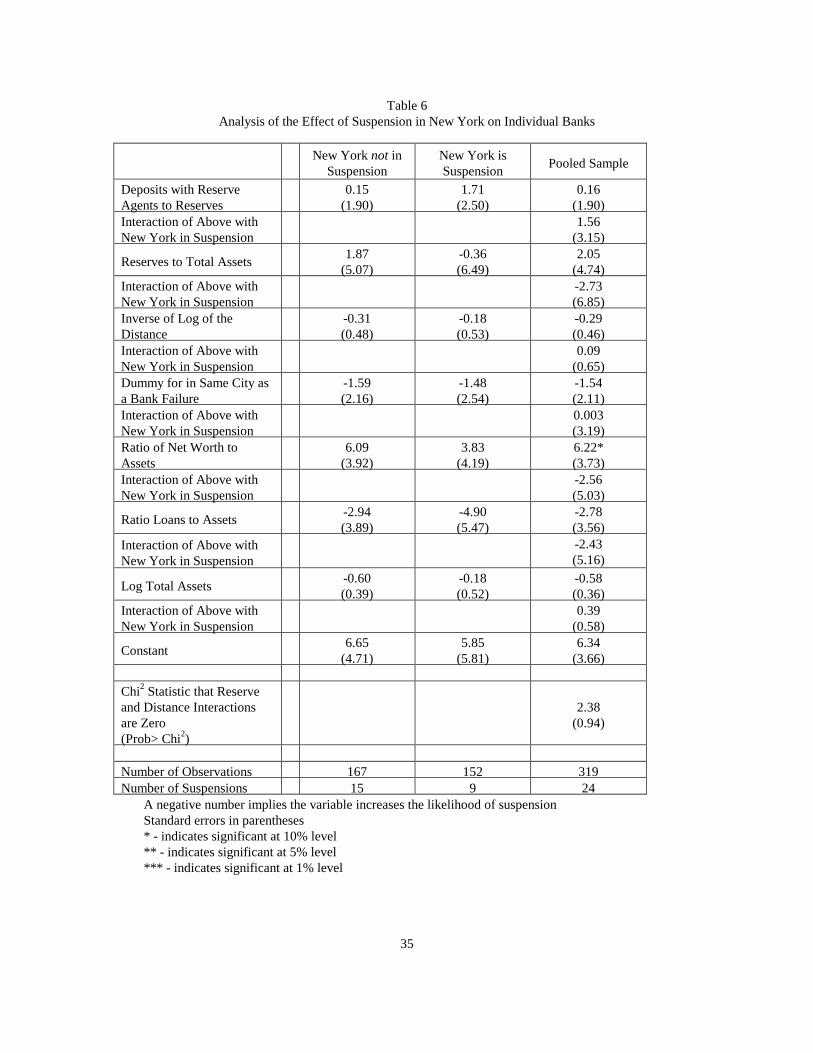
35

Table 6 Analysis of the Effect of Suspension in New York on Individual Banks

New York not in

Suspension New York is Suspension Pooled Sample

Deposits with Reserve Agents to Reserves

0.15 (1.90)

1.71 (2.50)

0.16 (1.90)

Interaction of Above with New York in Suspension

1.56 (3.15)

Reserves to Total Assets 1.87 (5.07)

-0.36 (6.49)

2.05 (4.74)

Interaction of Above with New York in Suspension

-2.73 (6.85)

Inverse of Log of the Distance

-0.31 (0.48)

-0.18 (0.53)

-0.29 (0.46)

Interaction of Above with New York in Suspension

0.09 (0.65)

Dummy for in Same City as a Bank Failure

-1.59 (2.16)

-1.48 (2.54)

-1.54 (2.11)

Interaction of Above with New York in Suspension

0.003 (3.19)

Ratio of Net Worth to Assets

6.09 (3.92)

3.83 (4.19)

6.22* (3.73)

Interaction of Above with New York in Suspension

-2.56 (5.03)

Ratio Loans to Assets -2.94 (3.89)

-4.90 (5.47)

-2.78 (3.56)

Interaction of Above with New York in Suspension

-2.43 (5.16)

Log Total Assets -0.60 (0.39)

-0.18 (0.52)

-0.58 (0.36)

Interaction of Above with New York in Suspension

0.39 (0.58)

Constant 6.65 (4.71)

5.85 (5.81)

6.34 (3.66)

Chi2 Statistic that Reserve and Distance Interactions are Zero (Prob> Chi2)

2.38 (0.94)

Number of Observations 167 152 319 Number of Suspensions 15 9 24

A negative number implies the variable increases the likelihood of suspension Standard errors in parentheses * - indicates significant at 10% level ** - indicates significant at 5% level *** - indicates significant at 1% level