Bank Fragility, “Money under the Mattress,” and Long-Run GrowthU.S. Evidence from the “Perfect” Panic of 1893

Carlos D. Ramirez

George Mason University

FDIC’s Center for Financial Research

Finance-Growth Nexus: A debate with a long history… Schumpeter: “The banker…authorizes

people, in the name of society as it were, to…[innovate]” (Theory of Economic Development, 1911)

Joan Robinson (1952) argues that finance simply responds to growth.

Question still being investigated… Kroszner, Laeven, and Klingebiel (2005); Dell’Ariccia, Detragiache, and Rajan

(2005); Bonfiglioli and Mendicino (2004); Levine (2005); Rajan and Zingales (1998), etc.

Objects of this paper:

1. Estimates interstate growth regressions to examine the impact of bank failures and banking organization on long-run growth.

2. Provides a simple, intuitive framework for understanding how or why bank failures can affect growth in the long run.

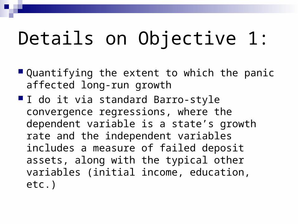
Details on Objective 1:

Quantifying the extent to which the panic affected long-run growth

I do it via standard Barro-style convergence regressions, where the dependent variable is a state’s growth rate and the independent variables includes a measure of failed deposit assets, along with the typical other variables (initial income, education, etc.)

Why 1893?

It happened a long time ago--useful for understanding its long-run consequences.

Panic was very severe. Lots of bank failures. Output contraction was very severe--2nd only to the Great

Depression. Incidence of bank failures varied significantly among states--

allows for identification of effects. Bank failures were not directly caused by local adverse

economic conditions--mitigates possible endogeneity problems.

No federal government response that may “contaminate” the results.

Basic Results1900-1930 Growth Regressions

Variable OLS WLS: Population 1900 WLS: Income 1900

Initial income -0.021 -0.021 -0.021 -0.006 -0.010 -0.016 -0.013 -0.015 -0.020

(0.004) (0.004) (0.004) (0.005) (0.006) (0.005) (0.006) (0.005) (0.004)

0.000 0.000 0.000 0.277 0.108 0.004 0.035 0.005 0.000

Illiteracy rate -0.060 -0.052 -0.041 -0.036 -0.038 -0.043 -0.053 -0.053 -0.052

(0.014) (0.013) (0.014) (0.017) (0.017) (0.016) (0.019) (0.017) (0.016)

0.000 0.000 0.006 0.047 0.025 0.011 0.008 0.003 0.002

Banking instability -0.043 -0.031 -0.018 -0.053 -0.042 -0.024 -0.059 -0.046 -0.029

(0.015) (0.013) (0.013) (0.012) (0.012) (0.011) (0.013) (0.012) (0.012)

0.006 0.023 0.196 0.000 0.002 0.046 0.000 0.000 0.024

Branching allowed? 0.006 0.006 0.005 0.006 0.006 0.002 0.006 0.007 0.002

(0.002) (0.002) (0.002) (0.003) (0.003) (0.002) (0.003) (0.003) (0.002)

0.012 0.017 0.037 0.033 0.026 0.295 0.035 0.024 0.248

Bank density 0.165 -0.009 0.124 -0.039 0.129 -0.038

(0.103) (0.098) (0.080) (0.074) (0.076) (0.066)

0.118 0.924 0.131 0.600 0.098 0.578

Financial depth 0.100 0.090 0.085

(0.032) (0.018) (0.017)

0.002 0.000 0.000

Adjusted R-Squared 0.466 0.526 0.604 0.351 0.384 0.524 0.425 0.467 0.596

F statistic 10.130 10.800 12.290 6.320 5.710 15.610 6.630 7.130 15.920

Prob>F 0.000 0.000 0.000 0.001 0.001 0.000 0.000 0.000 0.000

Num of Observations 45 45 45 45 45 45 45 45 45

Are coefficients meaningful?1900-1930 Growth Regressions: Implied Elasticities

Variable OLS WLS: Population 1900 WLS: Income 1900

Initial income -0.584 -0.594 -0.587 -0.163 -0.245 -0.398 -0.314 -0.383 -0.488

0.114 0.100 0.108 0.148 0.149 0.130 0.145 0.128 0.118

0.000 0.000 0.000 0.274 0.102 0.002 0.030 0.003 0.000

Illiteracy rate -0.159 -0.140 -0.110 -0.083 -0.089 -0.099 -0.082 -0.083 -0.082

0.037 0.035 0.038 0.041 0.038 0.037 0.029 0.025 0.024

0.000 0.000 0.003 0.041 0.020 0.008 0.005 0.001 0.001

Banking instability -0.053 -0.038 -0.022 -0.041 -0.033 -0.019 -0.048 -0.038 -0.023

0.018 0.016 0.016 0.009 0.009 0.009 0.010 0.010 0.010

0.004 0.019 0.185 0.000 0.001 0.041 0.000 0.000 0.020

Branching allowed? 0.063 0.060 0.048 0.046 0.049 0.016 0.048 0.053 0.015

0.024 0.023 0.022 0.020 0.020 0.014 0.021 0.023 0.013

0.009 0.012 0.030 0.025 0.019 0.291 0.026 0.016 0.245

Bank density 0.046 -0.003 0.039 -0.012 0.048 -0.014

0.029 0.028 0.025 0.023 0.028 0.024

0.108 0.923 0.122 0.598 0.088 0.576

Financial depth 0.138 0.129 0.146

0.044 0.028 0.030

0.002 0.000 0.000

What does it all mean?

States that experienced more banking failures (whether temporary or permanent), grew less rapidly, certeris paribus.

The effect of bank disintermediation is nearly as large as that of eliminating geographical restrictions in banking.

Standing back for a second…

Literature that studies the effects of banking crises on economic activity focuses on short-run effects.

Here I am arguing that there may be long-term effects as well.

What may explain these long-term effects?

Now, looking at Objective 2:

Depositors do not know if or when they will get their money back from a closed bank.

Bank closures (temporary or permanent) induces a reaction from ALL depositors.

With bank failures, depositors lose confidence on banking system.

Prefer to keep the money “hidden under the mattress.”

If this becomes “institutionalized” it will affect LR growth.

Looking for more evidence: comparing WV and NE Why is this comparison interesting? WV did not see a single bank failure during

the 1893 panic, even though it was a very poor state.

NE experienced the second highest bank failure rate in terms of deposits. It was the first in terms of bank failure rate.

So it is like comparing the best with the worst.

What do we see?Growth of Bank Deposits for State Banks: Nebraska versus West Virginia

-1.000

-0.500

0.000

0.500

1.000

1.500

2.000

2.500

3.000

3.500

1890 1892 1894 1896 1898 1900 1902 1904 1906 1908 1910 1912 1914 1916 1918 1920 1922 1924 1926 1928 1930

Nebraska

West Virginia

NE introduces DI

Evidence for portfolio (de-) composition Survey evidence: Czech Republic survey on March 2003: 75%

of population do not trust banks. Argentina, 2004, a survey done by American

Express, reveals 86% population do not trust banks.

The Moscow Times reports in 2004 that approximately 70% of population do NOT have bank accounts!

US bank in the 1890s?

Evidence presented is for modern times. Imagine what it must have been like back

in the 1890s… Some evidence: newspapers

Some newspaper evidence

Chicago Daily Tribune, March 21, 1895: Indiana “miser” dies with about $15,000 in gold and cash hidden around his house. (nearly $400,000 in today’s dollars.)

New York Times, May 17, 1897 reports: “Mr. Bissel, a farmer, having no faith in banks, kept his money hidden about his farm…The other day he hid it up in flue. The next day his wife put up a stove and started a fire and burned up $3,000 in bank notes.”

New York Times, Nov. 1, 1901 reports: “Jacob Nickelson, who lives near Hyndman, did not believe in banks, and kept his money hidden in his house. Yesterday robbers stole $4,500 in greebacks.”

Washington Post, June 25, 1905 reports: “The bank commissioner of Kansas is quoted as saying that while there is no way of getting accurate figures, he has reason to believe that there is as much money hidden in socks and under carpets or buried or carried as is on deposits, and Commissioner Royce, of Nebraska, agrees with his opinion….”

Time Series Evidence…

Pictures and articles are suggestive, but inconclusive.

Need more “hard” evidence. Look at newspaper articles more closely. Downloaded ALL newspaper articles between

1860 and 1970 that had the words: “money hidden.”

Majority of articles are tales of people losing their wealth in fires, robberies, accidents, etc.

Newspaper evidence…

Search produced 641 articles.

Look at the incidence of articles over time:

tt

n

iitit FDICpostcrisisYearMH

2

010

“Money Hidden”—Results:

n = 2 n = 4 n = 6 n = 8 n = 10 Year 0.033 0.032 0.033 0.033 0.033 (0.003) (0.004) (0.004) (0.004) (0.004) 0.000 0.000 0.000 0.000 0.000

Crisist ii0

n

0.807 1.249 1.837 2.840 3.665

(0.331) (0.452) (0.536) (0.635) (0.693) 0.016 0.007 0.001 0.000 0.000 Post-FDIC -1.663 -1.553 -1.553 -1.498 -1.496 (0.245) (0.259) (0.257) (0.254) (0.251) 0.000 0.000 0.000 0.000 0.000 Num. Obs. 109 107 105 103 101 F-test 22.64 15.10 11.93 10.07 8.71 Prob>F 0.000 0.000 0.000 0.000 0.000 Adj. R Sqrd. 0.501 0.482 0.486 0.495 0.501

Allowing of Lagged Dep. Vbl: n = 2 n = 4 n = 6 n = 8 n = 10 Lagged dep. vbl. 0.411 0.406 0.398 0.347 0.290 (0.085) (0.089) (0.088) (0.093) (0.098) 0.000 0.000 0.000 0.000 0.004 Year 0.020 0.020 0.020 0.022 0.024 (0.004) (0.004) (0.004) (0.005) (0.005) 0.000 0.000 0.000 0.000 0.000

Crisist ii0

n

0.644 0.760 1.222 1.916 2.638

(0.302) (0.427) (0.508) (0.645) (0.750) 0.035 0.078 0.018 0.004 0.001 Post-FDIC -0.985 -0.950 -0.970 -1.011 -1.090 (0.263) (0.271) (0.268) (0.272) (0.277) 0.000 0.001 0.000 0.000 0.000 Implied LT elas. 1.092 1.281 2.029 2.934 3.718 (0.519) (0.696) ((0.816) (0.912) (0.937) 0.038 0.069 0.015 0.002 0.000 Num. Obs. 109 107 105 103 101 F-test 26.77 18.38 14.90 11.66 9.43 Prob>F 0.000 0.000 0.000 0.000 0.000 Adj. R Sqrd. 0.589 0.567 0.572 0.556 0.541

Conclusion

The amount of disintermediation caused by bank failures and bank panics can be quite substantial.

The effect of disintermediation can go beyond the standard short-run “credit crunch” stories.

Disintermediation, without some sort of policy intervention aimed at restoring faith in the banking system, can have long-term consequences for growth.