Categorical Data Analysis (for R-avoiders) · Overview Block 1 Categorical data analysis using hierarchical log-linear models in SPSS/PASW Advantages/disadvantages using this approach

Categorical Data Analysis

(for R-avoiders)

Christoph Scheepers

Glasgow

Intro Linear Mixed Models (LME)

Discussed in two (orthogonal!) contexts

Simultaneous generalisation of effects across subjects and items

(better alternative to calculating min. F’ from F1 and F2, cf

Clark 1973)

Providing adjustments (i.e. distribution and link functions) for a

wider range of analysis problems, including categorical data

analysis (cf. Jaeger, 2008, JML)

For the categorical data problem, alternatives to

LME are available!

Hierarchical log-linear models

Generalized Estimating Equations

Logistic Regression

Etc.

Overview

Block 1

Categorical data analysis using hierarchical log-linear models

in SPSS/PASW

Advantages/disadvantages using this approach

Examples/Demos

Block 2

Categorical data analysis using Generalized Estimating

Equations (GEE) in SPSS/PASW

Very similar to LME, actually

distribution & link functions

Inclusion of continuous predictors (covariates)

No „random effects‟, but instead classical distinction between

“within” and “between” factors (mixed designs are no problem)

Examples/Demos

Overview

Block 3

Linear Mixed Effects Models (LME) in SPSS/PASW

In SPSS/PASW, no distribution/link functions as yet (hence, can

only be applied to normally distributed continuous data)

BUT, can be used to address the subject/item generalization issue

Specifying „proper‟ LME random models

Comparison to classical F1, F2, min. F‟ approach

Potential problems

Log-linear Analysis

Christoph Scheepers

The Problem Measurement at nominal scale level

e.g., discrete response categories like “agree”, ”disagree”,

“don‟t know”..

agree disagree don’t know Total

Condition A 35 28 22 85

Condition B 48 17 35 100

Condition C 22 42 26 90

Condition D 30 40 24 94

Total 135 127 107 N = 369

Possible Solution

Summarize data as „probabilities per condition‟ and

run parametric test (e.g. ANOVA including condition

and response category as factors)

agree disagree don’t know

mean variance mean variance mean variance

Condition A 0.41 0.25 0.33 0.22 0.26 0.19

Condition B 0.48 0.25 0.17 0.14 0.35 0.23

Condition C 0.24 0.19 0.47 0.25 0.29 0.21

Condition D 0.32 0.22 0.43 0.25 0.26 0.19

However…

Such an approach would clearly violate the

requirements for parametric testing (ANOVA or t-test):

Normality: a normal distribution ranges from –infinite to

+infinite, but probabilities range from 0 to 1!

Linear independence of factor levels: response category

cannot be considered a factor because means would, of

necessity, be negatively correlated (they always add up to 1

across levels)!

Homogeneity of variance: variances become systematically

smaller as means approach one of the „boundaries‟ (0 or 1)!

Interaction or not?

In terms of differences (cf. ANOVA), there would be an interaction

between A and B (40-20=20 vs. 20-10=10)

Proportionally (in terms of %-ratios), there is no interaction

(40/20=2 vs. 20/10=2), just two main effects (A.2 increases

proportions by a factor of 2 and so does B.1)

20%

40%

10%

20%

0%

10%

20%

30%

40%

50%

1 2

A

B 1

B 2

Categorical data: relationship between mean and variance

0

0.1

0.2

0.3

0.4

0.5

1 0.95 0.9 0.85 0.8 0.75 0.7 0.65 0.6 0.55 0.5 0.45 0.4 0.35 0.3 0.25 0.2 0.15 0.1 0.05 0

mean probability of "yes" responses

max. vari

an

ce

Homogeneity of Variance?

The maximum expected variance becomes smaller as the

mean approaches 0 or 1; it is expected to be highest around

a mean of 0.5.

Arcsine-(sqrt) transformation(?)

p‟i → arsin √pi When xi = pi which is a probability

Inverse: sin p‟i2

arcsine-sqrt as function of probability

arcsine(sqrt(P))

0

0.2

0.4

0.6

0.8

1

1.2

1.4

1.6

0 0.1 0.2 0.3 0.4 0.5 0.6 0.7 0.8 0.9 1

Series1

Logit transformation

p‟i → ln(pi/(1-pi)) When xi = pi which is a probability

Inverse: exp(p‟i/(1+exp(p‟i)))

logits as function of probability

ln(P / (1 - P))

-6

-4

-2

0

2

4

6

0 0.1 0.2 0.3 0.4 0.5 0.6 0.7 0.8 0.9 1

Series1

A Non-Parametric Solution transformation etc. NOT REQUIRED

The Pearson chi-square test for two independent samples

(also called cross-tabulation or contingency table analysis)

Tests whether two discrete variables are independent of one

another (if so, observed frequencies in the cells should be

proportional to the column and row totals).

VAR. 1



VAR. 2 Condition B 48 17 35 100



Total 135 127 107 N = 369

Pearson Chi-Square Test Expected frequencies under H0 (stating that both variables are

independent)

For each design cell, multiply the appropriate row-total with the

appropriate column-total and divide the result by N (overall

number of observations).

VAR. 1






Total 135 127 107 N = 369

31.1 29.3 24.6

36.6 34.4 29.0

32.9 31.0 26.1

27.3 32.4 34.4

The underlying logic

Combined probabilities/likelihoods/frequencies of independent

events multiply!

If, say, the probability of a person wearing blue jeans is 0.4 and the

probability of a person wearing a white t-shirt is 0.1, then the

probability of a person wearing both blue jeans AND a white t-shirt

is 0.4 × 0.1 = 0.04 … (assuming that the choice of t-shirt is

independent of the choice of blue jeans).

Expected frequencies in Chi-square tests follow exactly the same

logic

Any systematic deviation from the independence assumption (i.e.

systematic deviations from the Eis) indicates that the two variables

are NOT independent from one another, i.e. that VAR.1 somehow

influences VAR.2 (or vice versa)

Pearson Chi-Square Test Chi-square statistic: 2 = (Oi – Ei)

2 / Ei

where Oi refers to the observed and Ei to the expected frequency in design cell i.

2 = (35 – 31.1)2 / 31.1 + (28 – 29.3)2 / 29.3 + (22 – 24.6)2 / 24.6 + (48 – 36.6)2 / 36.6 +

(17 – 34.4)2 / 34.4 + (35 – 29.0)2 / 29.0 + (22 – 32.9)2 / 32.9 + (42 – 31.0)2 / 31.0 +

(26 – 26.1)2 / 26.1 + (30 – 34.4)2 / 34.4 + (40 – 32.4)2 / 32.4 + (24 – 27.3)2 / 27.3

= 24.674; df = (rows-1)*(columns-1) = 2*3 = 6; p < .001

VAR. 1






Total 135 127 107 N = 369

31.1 29.3 24.6

36.6 34.4 29.0

32.9 31.0 26.1

27.3 32.4 34.4

Likelihood Ratio Test Likelihood ratio chi-square: LR2 = 2 * Oij * ln(Oij/Eij)

where Oij refers to the observed and Eij to the expected frequency in design cell ij

(row/column).

LR2 =2 * (35 * ln(35/31.1) + 28 * ln(28/29.3) + 22 * ln(22/24.6) + 48 * ln(48/36.6) +

17 * ln(17/34.4) + 35 * ln(35/29.0) + 22 * ln(22/32.9) + 42 * ln(42/31.0) +

26 * ln(26/26.1) + 30 * ln(30/34.4) + 40 * ln(40/32.4) + 24 * ln(24/27.3)

= 26.108; df = (rows-1)*(columns-1) = 2*3 = 6; p < .001

VAR. 1






Total 135 127 107 N = 369

31.1 29.3 24.6

36.6 34.4 29.0

32.9 31.0 26.1

27.3 32.4 34.4

)

Equivalent to Pearson Chi2

(given large sample size)

Requirements

(2, LR2, log-linear models)

Rules of thumb (if not met, statistics may

become overly conservative):

All design cells must have expected

frequencies (Eij) greater than 1

At least 80% of the design cells must have Eijs

greater than 5.

No further requirements! (Parameter-free

statistics)

Hmm.. The procedures discussed so far have only looked at two-

dimensional tables. In fact, it is not possible to apply the Pearson

Chi-Square test to tables with more than two dimensions!

So, do we have to use ANOVA (of which we know it is not

appropriate for categorical data) in case of multi-way tables (three

or more discrete variables)?

Fortunately, the answer is NO because of the existence of

LOGLINEAR MODELS. These combine features of

Chi-square tests (determining the fit between observed and expected

frequencies)

ANOVA (simultaneous testing of main effects and interactions within a

multi-factorial design)

Indeed, it is even possible to perform by-subject/item analyses in log-

linear models!

Log-linear Models Apply to all kinds of n-way contingency tables.

Let‟s stick to our two-way example first before moving on to a three-way

table:

A different way of conceptualising the data: There is a main effect

of VAR.1 (column sums), a main effect of VAR.2 (row sums), and an

interaction (individual cell frequencies) – NB: only the latter is actually

being tested in a standard chi-square test.

VAR. 1






Total 135 127 107 N = 369

Log-linear Models

Recall from ANOVA the following modelling

assumption:

Xij = + i + j + ij + e

i.e., any observation (Xij) can be predicted in terms of

a linear combination of the grand mean (), the main

effect of factor A at level i (i = Ai - ), the main effect

of factor B at level j (j = Bj - ), the interaction

between Ai and Bj (ij = Xijk - Ai - Bj + ), and finally,

some error (e).

Log-linear Models

Log-linear models (similar to chi-square tests),

however, assume multiplicative relationships:

nij = N * i * j * ij

i.e., any cell count (nij) can be predicted as the

product of the overall number of observations (N)

times the main effect of variable A at level i (i = nAi /

N), the main effect of variable B at level j (j = nBj / N),

and the interaction between Ai and Bj (ij = nij / nAi /

nBj * N).

Note that there is no error term because we model

cell counts (there is no within-cell variance).

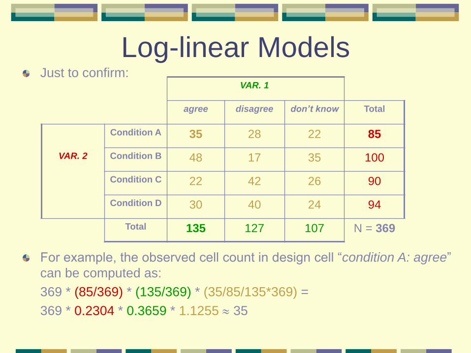
Log-linear Models Just to confirm:

For example, the observed cell count in design cell “condition A: agree”

can be computed as:

369 * (85/369) * (135/369) * (35/85/135*369) =

369 * 0.2304 * 0.3659 * 1.1255 35

VAR. 1






Total 135 127 107 N = 369

Log-linear Models

However, a multiplicative model can be easily

translated into a linear (i.e. additive) one via a

logarithm transformation, since:

log(A*B) = log(A) + log(B); log(A/B) = log(A) – log(B)

(Note: logB(X) = Y BY = X)

Thus, we can restate our multiplicative model in

linear terms:

ln(nij) = ln(N) + ln(i) + ln(j) + ln(ij)

(by convention, the “natural log” (ln) is being used, i.e. the log to the

base of 2.718281846 (Euler‟s number) – no idea why this is called

“natural”, btw. …)

Again, just to confirm:

For example, the natural log of the observed cell count in design cell

“Condition A: agree” can be computed as:

5.911 + (4.443 – 5.911) + (4.905 – 5.911) + (3.555 – 4.443 – 4.905 + 5.911) =

5.911 – 1.468 – 1.006 + 0.118 = 3.555

VAR. 1


Condition A 3.555 3.332 3.091 4.443

VAR. 2 Condition B 3.871 2.833 3.555 4.605

Condition C 3.091 3.738 3.258 4.500

Condition D 3.401 3.689 3.178 4.543

Total 4.905 4.844 4.673 5.911

Log-linear Models

Is there a significant main effect of VAR. 2?

Expected log frequencies: ln(369/4) in each condition

Compute likelihood ratio chi square: LR2 = 2* eln(Oi) * (ln(Oi) – ln(Ei)) =

2 * ( 85 * (4.443 – 4.525) + 100 * (4.605 – 4.525) + 90 * (4.5 – 4.525)

+ 94 * (4.543 – 4.525) ) = 0.928, df = 3; p = .82 (n.s.)

VAR. 1

agree disagree don’t know Total Obs. Total Exp.

Condition A 3.555 3.332 3.091 4.443 4.525

VAR. 2 Condition B 3.871 2.833 3.555 4.605 4.525

Condition C 3.091 3.738 3.258 4.500 4.525

Condition D 3.401 3.689 3.178 4.543 4.525

Total 4.905 4.844 4.673 5.911

Log-linear Model TESTING

Is there a significant interaction between VAR.1 and VAR.2?

Expected log frequencies: row + column – overall (cf. classical 2 test)

Compute likelihood ratio chi square: LR2 = 2* eln(Oi) * (ln(Oi) – ln(Ei)) =

26.546; df = 6; p < .001 (with more precision, it would be the same result

as in the classical likelihood ratio chi-square section)

VAR. 1


Condition A 3.555 3.332 3.091 4.443

VAR. 2 Condition B 3.871 2.833 3.555 4.605

Condition C 3.091 3.738 3.258 4.500

Condition D 3.401 3.689 3.178 4.543

Total 4.905 4.844 4.673 5.911

Log-linear Model TESTING

Note: model tested is

ln(N) + ln() + ln()

3.437 3.376 3.205

3.599 3.538 3.367

3.494 3.433 3.262

3.537 3.476 3.305

Log-linear Models Hierarchical approach to hypothesis testing

in order to test the interaction between two variables, A and B, we

test the “goodness of fit” of a model that contains only the main effect

of A and the main effect of B.

A “bad fit” of that model results in a significant LR2 statistic, and we

conclude that the interaction must be considered to fit the data.

The same logic can be applied to multidimensional tables

in order to test, say, a three-way interaction between variables A, B,

and C, we test the goodness of fit of a model containing only two-way

interactions (A*B and A*C and B*C).

If the model containing only 2-way interactions doesn‟t fit (significant

LR2 ) we conclude that the three-way interaction (A*B*C) must be

considered, and so forth…

Effect Hierarchies A * B * C * D

A * B * C B * C * D A * C * D A * B * D

A * B B * C C * D A * C A * D B * D

A B C D

Ø

4-way interaction

3-way interactions

2-way interactions

main effects

no effect

Thus, in order to test whether, e.g., A*B*C is significant, we test the goodness of fit

of a model containing A*B and B*C and A*C (and the corresponding lower order effects)!

Is there a significant interaction between VAR.1, VAR.2, and VAR.3?

3*2*2 design (same raw cell frequencies as before, but partitioned in a

different way)

In order to calculate expected frequencies for the 3-way interaction, we

have to refer to sub-tables representing the relevant 2-way interactions

(by computing the appropriate sums across design cells)…

Testing a 3-way interaction

1

2

VAR. 1

VAR. 2 VAR. 3 agree disagree don’t know

A 35 (3.555) 28 (3.332) 22 (3.091)

B 48 (3.871) 17 (2.833) 35 (3.555)

A 22 (3.091) 42 (3.738) 26 (3.258)

B 30 (3.401) 40 (3.689) 24 (3.178)

VAR. 1

VAR. 2 agree disagree don‟t know Total

1 83 (4.419) 45 (3.807) 57 (4.043) 185 (5.220)

2 52 (3.951) 82 (4.407) 50 (3.912) 184 (5.215)

Total 135 (4.905) 127 (4.844) 107 (4.673) 369 (5.911)

VAR. 1

VAR. 3 agree disagree don‟t know Total

A 57 (4.043) 70 (4.248) 48 (3.871) 175 (5.165)

B 78 (4.357) 57 (4.043) 59 (4.078) 194 (5.268)

Total 135 (4.905) 127 (4.844) 107 (4.673) 369 (5.911)

VAR. 3

VAR. 2 A B Total

1 85 (4.443) 100 (4.605) 185 (5.220)

2 90 (4.500) 94 (4.543) 184 (5.125)

Total 175 (5.165) 194 (5.268) 369 (5.911)

The relevant 2-way interactions marginal association tables: Example cell:

VAR.1 * VAR.2 Interaction:

4.419 – 5.220 – 4.905

+ 5.911 = 0.205


4.043 – 5.165 – 4.905

+ 5.911 = – 0.116


4.443 – 5.220 – 5.165

+ 5.911 = – 0.031

VAR.1 main effect:

4.905 – 5.911 = –1.006

VAR.2 main effect:

5.220 – 5.911 = –0.691

VAR.3 main effect:

5.165 – 5.911 = –0.746

Applied to each design cell, we obtain the following expected ln

frequencies (small numbers). (Large numbers represent ln observed

frequencies):

Expected ln frequency for design cell agree:1:A

E(agree:1:A) = 5.911 – 1.006 – 0.691 – 0.746 + 0.205 – 0.116 – 0.031 = 3.526

LR2 etc.: see brief SPSS tutorial...

Testing a 3-way interaction

VAR. 1

VAR. 2 VAR. 3 agree disagree don’t know

A 3.555 3.332 3.091

B 3.871 2.833 3.555

A 3.091 3.738 3.258

B 3.401 3.689 3.178

3.526 1

2

3.180 3.210

3.899 3.034 3.476

3.210 3.932 3.231

3.464 3.667 3.378

Marginal Associations 4-way interaction

3-way interactions

2-way interactions

main effects

no effect

In order to test whether, e.g., A*B*C is significant, we test the goodness of fit

of a model containing A*B and B*C and A*C (plus the corresponding lower order effects)!

A * B * C * D

A * B * C B * C * D A * C * D A * B * D

A * B B * C C * D A * C A * D B * D

A B C D

Ø

4-way interaction

3-way interactions

2-way interactions

main effects

no effect

In order to test whether, e.g., A*B*C is significant, we test the goodness of fit of a model

containing everything (from the same level downwards) except the effect of interest!

Partial Associations A * B * C * D

A * B * C B * C * D A * C * D A * B * D

A * B B * C C * D A * C A * D B * D

A B C D

Ø

4-way interaction

3-way interactions

2-way interactions

main effects

no effect

If subjects (or items) are included as factors, partial association tests will adjust

expected frequencies for inter-individual variation (cf. repeated-measures ANOVA)

Partial Associations: Within Subjects (Items)

A * B * C * S

A * B * C B * C * S A * C * S A * B * S

A * B B * C C * S A * C A * S B * S

A B C S

Ø

Summary and Conclusion Whenever you want to test interactions between three or more categorical

variables, log-linear analysis might be the right thing to do.

Log-linear models combine features of standard chi-square tests

(determining the fit between observed and expected cell counts) with

those of ANOVA (simultaneous testing of main effects and interactions

within multi-factorial designs).

They do not differentiate between „dependent‟ and „independent‟

variables (the response variable is always treated as a factor!).

They are applicable to the multinomial case (not only binary

response categories! Cf. LME, GEE discussed later)

Almost no requirements (except that the sample has to be sufficiently

large).

They can be used in an “explorative” model-building fashion (find the most

parsimonious model that describes the data best) as well as for

hypothesis testing (simultaneous testing of all possible factor

combinations).

New Problem(s):

Knowing that there is an interaction, we want to know, for

example, whether each response category is significantly

affected by condition (VAR.2), and whether proportions of

“agree” responses differ significantly from each other

across conditions (i.e., levels of VAR.2).

Hence, we must perform some equivalent of planned

comparisons (decomposing the interaction into its

underlying “simple effects”). (The same we would have to

do in a classical chi-square test).

This is, in principle, very similar to ANOVA, except that

there are some caveats …

Test “simple main effect” of condition (VAR.2) at each level of “response

category” (VAR.1).

The problem with such an approach would be that it would not take non-

occurrences into account: We are not interested in differences between

absolute frequencies (e.g. whether 35 [3.555] is different from 48 [3.871])

but rather in proportional differences (i.e. whether, e.g., 35/85 [3.555 –

4.443] is different from 48/100 [3.871 – 4.650])!

VAR. 1


Condition A 35 (3.555) 28 (3.332) 22 (3.091) 85 (4.443)

VAR. 2 Condition B 48 (3.871) 17 (2.833) 35 (3.555) 100 (4.605)

Condition C 22 (3.091) 42 (3.738) 26 (3.258) 90 (4.500)

Condition D 30 (3.401) 40 (3.689) 24 (3.178) 94 (4.543)

Total 135 (4.905) 127 (4.844) 107 (4.673) 369 (5.911)

The Wrong Approach!!

Summarise table by collapsing across response category levels that are not of

interest (dummy level “OTHER”) and look at the interaction between dummy-

VAR.1 and VAR.2!

This approach preserves the marginal and overall totals.

Note that “agree” and “REST” are complementary (they sum up to yield the

marginal totals of the original table).

The interaction between dummy-VAR.1 and VAR.2 therefore tells us about the

proportional change in # “agree” responses, dependent on condition (VAR.2).

dummy VAR. 1

agree REST Total

Condition A 35 (3.555) 50 (3.912) 85 (4.443)

VAR. 2 Condition B 48 (3.871) 52 (3.951) 100 (4.605)

Condition C 22 (3.091) 68 (4.220) 90 (4.500)

Condition D 30 (3.401) 64 (4.159) 94 (4.543)

Total 135 (4.905) 234 (5.455) 369 (5.911)

The Correct Approach!!

Useful Reading

Howell, D.C. (2002). Statistical Methods for Psychology

(5th edition). Pacific Grove, CA: Duxbury.

Chapter “Categorical Data and Chi-Square”

Chapter “Log-linear Analysis”

SPSS Demo Scheepers (under revision). Cross-structural priming of relative clause

attachments: implications for the mental representation of syntax.

Journal of Memory and Language.

Experiment 2:

Primes HA The knights jousted for [the daughter of the king]‟s … (e.g. “hand)

LA The knights jousted for the hand of [the king]‟s … (e.g. “daughter”)

BL The knights jousted for the daughter of the king when …

Targets The tourist guide mentioned the bells of the church that …

Coding: - Subject-ID (N=30)

- Subject Gender (0=male, 1=female)

- Item-ID (N=24)

- Prime (1=HA, 2=LA, 3=BL)

- Target-Attach (1=HA, 2=LA, 3=UC)

- Internal Target-Syntax (1=Subject-RC, 2=Object-RC, 3=Other)

- position of trial (in experiment)

First Demo

Find out whether there is a reliable effect of Prime

on the distribution of Target Attachments (Prime *

TargetAttach interaction) that can be generalised

across subjects and items

If so, which TargetAttach response categories (HA, LA,

UC) are primarily affected?

In relation to the BL prime condition, does the HA

prime condition reliably boost proportions of HA

TargetAttachments; does the LA prime condition reliably

boost proportions of LA target attachments?

Problem(?)

Prime * TargetAttach reliably interacted with

both subject and item (i.e. there were

significant subj*prime*target and

item*prime*target interactions)

Indeed, this should restrict our interpretation

in terms of generalizability of effects: see

next slide…

One way to think about it..

subject1 subject2

condA

condB

Effect is significant + its interaction

with subject/item is NOT significant

=> we can generalise both the

direction and the magnitude of the

effect across subjects/items

subject1 subject2

condA

condB

Effect is significant + its interaction

with subject/item is significant => we

can generalise the direction but not

the magnitude of the effect across

subjects/items

subject1 subject2

condA

condB

Effect is NOT significant + its

interaction with subject/item is

significant => we can neither

generalise the direction nor the

magnitude of the effect across

subjects/items

Cool stuff!

Because log-linear models (like Chi-Square) do not

distinguish between “dependent” and “independent”

variables (the distinction is only important when it comes to

interpretation!) one can

Include more than one “dependent variable” in the analysis

Even „cross‟ DVs with one another

Example Demo:

Crossing “target attachment” (HA vs. LA vs. UC) with “internal

structure of target” (Subj-RC vs. Object-RC vs. Other)

In principle, this is possible with other approaches as well

but it would require you to designate one of the DVs as

“DV” and the remaining DVs as “IVs” (predictors)

Not so cool stuff…

What about continuous predictors (covariates)?

No way to handle those other than by “categorical chunking” (e.g.

high, medium, low)

Better use logistic regression, GEE, or LME

Mixed Designs (including both “between” and “within” –

subject/item manipulations) won‟t work that well

Demo subject-analysis including participant-gender as predictor

Either fully between or fully within, but not both!

For mixed designs, better use GEE or LME

Conclusion

Hierarchical log-linear models are particularly useful for

The analysis of multi-dimensional (multi-factorial) categorical data

Categorical data with more than two levels (multinomial model), not

just binary data (binomial model)

Multi-dimensional DVs

They are probably not that useful for

Mixed designs (fully-within and fully-between designs are ok)

Designs with continuous predictors (covariates)

Results intercept-dev F1 df1 p1 F2 df2 p2 Min.F’ df p

Direction 69.483 1,38 .000 27.471 1,10 .000 19.685 1,19 .000

Pointsize 1.062 1,38 .309 1.674 1,10 .225 0.645 1,40 .425

Direction* Pointsize 0.000 1,38 .983 0.002 1,10 .970 0.000 1,48 .985

LME (S,I) LME (S,I,S*D,I*P)

intercept-dev F df p F df p

Direction 27.471 1,10 .000 23.322 1,14 .000

Pointsize 1.062 1,38 .309 0.678 1,34 .416

Direction* Pointsize 0.001 1,10 .971 0.001 1,34 .980

slope-dev F1 df1 p1 F2 df2 p2 Min.F’ df p

Direction 61.511 1,38 .000 33.568 1,10 .000 21.716 1,22 .000

Pointsize 1.663 1,38 .205 2.370 1,10 .155 0.977 1,38 .329



slope-dev F df p F df p

Direction 33.568 1,10 .000 27.166 1,15 .000

Pointsize 1.663 1,38 .205 0.942 1,35 .338


Results intercept-dev F1 df1 p1 F2 df2 p2 Min.F’ df p

Direction 69.483 1,38 .000 27.471 1,10 .000 19.685 1,19 .000

Pointsize 1.062 1,38 .309 1.674 1,10 .225 0.645 1,40 .425



intercept-dev F df p F df p

Direction 27.471 1,10 .000 23.322 1,14 .000

Pointsize 1.062 1,38 .309 0.678 1,34 .416


slope-dev F1 df1 p1 F2 df2 p2 Min.F’ df p

Direction 61.511 1,38 .000 33.568 1,10 .000 21.716 1,22 .000

Pointsize 1.663 1,38 .205 2.370 1,10 .155 0.977 1,38 .329



slope-dev F df p F df p

Direction 33.568 1,10 .000 27.166 1,15 .000

Pointsize 1.663 1,38 .205 0.942 1,35 .338


Documents

Categorical Data Analysis (for R-avoiders) · Overview Block 1 Categorical data analysis using hierarchical log-linear models in SPSS/PASW Advantages/disadvantages using this approach