Case Study: USEPA Benthic Invertebrate Risk Assessment for

Case Study: USEPA Benthic Invertebrate Risk

Assessment for Endosulfan

Prepared For: European Chemicals Agency Topical Scientific Workshop: Risk Assessment for the

Sediment Compartment 7-8 May, 2013

Helsinki, Finland

Prepared By: Keith Sappington

Senior Science Advisor Office of Pesticide Programs

U.S. Environmental Protection Agency Washington, DC, USA

Final 10 April 2013

2

CONTENTS Acknowledgments ........................................................................................................................................ 3

1. Background and Purpose ..................................................................................................................... 4

2. Problem Formulation ........................................................................................................................... 5

2.1 Nature of the Chemical Stressor ................................................................................................... 5

2.2 Assessment Endpoints and Conceptual Model ............................................................................. 7

2.3 Analysis Plan.................................................................................................................................. 9

3. Exposure Assessment ......................................................................................................................... 12

3.1 Modeled Sediment Concentrations ............................................................................................ 12

3.2 Monitored Sediment Concentrations ......................................................................................... 14

4. Effects Assessment ............................................................................................................................. 18

4.1 Sediment Toxicity Data ............................................................................................................... 18

4.2 Water Column Toxicity Data ....................................................................................................... 20

5. Risk Characterization .......................................................................................................................... 23

5.1 Predicted EECs vs. Sediment Toxicity Endpoints ........................................................................ 23

5.2 Monitored EECs vs. Sediment Toxicity Endpoints ....................................................................... 26

5.3 Pore Water EECs vs. Water Column Toxicity Endpoints ............................................................. 27

6. Discussion and Conclusions ............................................................................................................... 29

7. Cited Literature ................................................................................................................................... 32

Final 10 April 2013

3

ACKNOWLEDGMENTS The author acknowledges his co-authors of the USEPA 2010 Environmental Fate and Ecological Risk Assessment of Endosulfan: Dr. Mohammed Ruhman (ESEPA, OPP), Dr. Glen Thursby (USEPA, ORD), and Dr. Sandy Raimondo (USEPA, ORD). Without their valuable contributions, the 2010 assessment and this case study would not have been possible. The author also acknowledges Dr. Mah Shamim for her timely review of an earlier draft of this case study.

Final 10 April 2013

4

1. BACKGROUND AND PURPOSE This case study was prepared upon the request of the organizing committee of the European

Chemicals Agency (ECHA) Topical Scientific Workshop: Risk Assessment for the Sediment

Compartment, held 7-8 May, 2013 in Helsinki, Finland. Its primary purpose is to illustrate the

methods and data considered by the U.S. Environmental Protection Agency’s (USEPA), Office of

Pesticide Programs (OPP) in assessing pesticide risks to benthic invertebrates based on its

recent environmental fate and ecological risk assessment for the insecticide, endosulfan

(USEPA 2010).1 Using this case study, various benthic invertebrate risk assessment issues are

explored, including: (1) the choice of exposure media for expressing risk (pore water vs. bulk

sediment); (2) the selection of invertebrate species for characterizing toxicological effects; (3)

the role of monitoring data in benthic invertebrate risk assessment; and (4) the major sources

of uncertainty encountered in the risk assessment.

It should be recognized that endosulfan is considered a “data rich” chemical with regard to the

availability of ecological exposure and effects information relevant to benthic invertebrates.

While the breadth and depth of information available for endosulfan is not expected to be

available for most other chemicals of concern (especially industrial chemicals), this case study

provides an opportunity to evaluate the utility and robustness of various risk assessment

decisions and assumptions that must be made under “data poor” situations. It should also be

understood that the benthic invertebrate risk assessment was only one component of the

USEPA 2010 environmental fate and ecological risk assessment for endosulfan. Other

components included an evaluation of risks to birds, mammals, amphibians, pelagic

invertebrates, and plants in the context of both “near field” and “far field” (long range

transport) exposures. The USEPA 2010 endosulfan environmental fate and ecological risk

assessment was also part of a broader re-evaluation of the risks and benefits associated with

registered uses of endosulfan in the U.S., and therefore also included evaluation of health

effects, economic benefits, and available pesticide substitutes. Currently, endosulfan is being

voluntarily phased out from use in the U.S., with a permanent phase out expected over the next

several years.

1 available at: http://www.regulations.gov/#!documentDetail;D=EPA-HQ-OPP-2002-0262-0162;oldLink=false

http://www.regulations.gov/#!documentDetail;D=EPA-HQ-OPP-2002-0262-0162;oldLink=false

Final 10 April 2013

5

The following case study is organized by the main components considered in OPP ecological risk

assessments: Problem Formulation, Exposure Assessment, Effects Assessment and Risk

Characterization (USEPA 1998; USEPA 2004). Where appropriate, additional analyses have been

conducted in this case study to illustrate specific issues associated with assessing risks to

benthic invertebrates. In other cases, certain aspects of the risk assessment process are not

presented or are condensed for the purposes of brevity.

2. PROBLEM FORMULATION Problem formulation provides a strategic framework for the risk assessment. It sets the

objectives for the risk assessment, evaluates the nature of the problem, and provides a plan for

analyzing the data and characterizing the risk (US EPA 1998). Main components of the problem

formulation phase illustrated in this case study include: 1) defining the nature of the chemical

stressor, 2) developing the conceptual model, 3) selecting assessment and measurement

endpoints and 4) formulating the analysis plan.

2.1 Nature of the Chemical Stressor

Endosulfan (6,7,8,10,10-hexachloro-1,5,5a,6,9,9a-hexahydro-6,9-methano-2,4,3-

benzadioxathiepin 3-oxide) is a dioxathiepininsecticide and acaricide (broadly classified as an

organochlorine). The chemical is a 70:30 mixture of two biologically-active isomers (α and β)

and it acts as a contact poison to a wide variety of insects and mites through blockage of GABA-

(gamma amino butyric acid) gated chloride channels affecting nerve signals. Chemical

structures of α and β endosulfan and its major degradate, endosulfan sulfate, are shown in

Figure 1.

(the wedge bonds are used to indicate direction, not stereo-isomerism)

α-endosulfan (959-98-8) β-endosulfan (33213-65-9) Endosulfan Sulfate (1031-07-8)

Figure 1. Chemical stressors of ecological concern for agricultural applications of endosulfan

Final 10 April 2013

6

Stressor sources include foliar application of endosulfan formulated products prepared from

wettable powders and emulsifiable concentrates by air, ground and airblast application

methods. In an agricultural setting, major quantities of the applied pesticide active ingredient

reach target foliage and eventually end-up in the soil system. Smaller quantities of the applied

pesticide reach nearby field or water bodies initially by drift and then by runoff/erosion and by

volatilization. Based on submitted environmental fate data, biologically-mediated

transformation of α and β-endosulfan is expected to occur in the soil system producing

endosulfan sulfate (maximum observed levels ≈52% of applied material) which is a major

degradate of toxicological concern. Endosulfan sulfate is included with its two parents α and β-

endosulfan due to its similar toxicity as parent isomers and its formation as a “major”

degradate (e.g., > 10%) in aquatic and terrestrial systems. Endosulfan sulfate is also more

persistent than the parent isomers (α and β-endosulfan) and tends to be a major component of

total endosulfan residues found in biologically active environmental media (e.g., aerobic soil,

water, and sediments). Other degradates (endosulfan diol, endosulfan lactone and endosulfan

ether) were considered but ultimately excluded from the risk assessment in part because they

form in low quantities in the aquatic and terrestrial environment and available data suggest

they are less toxic2. For the purpose of this case study, the term “endosulfan” refers to the

technical grade active ingredient (TGAI), i.e. the combination of the α-endosulfan and β-

endosulfan isomers only, unless otherwise indicated. The term “total endosulfan” or

“endosulfans” refers to the combination of α-endosulfan, β-endosulfan and endosulfan

sulfate unless otherwise noted.

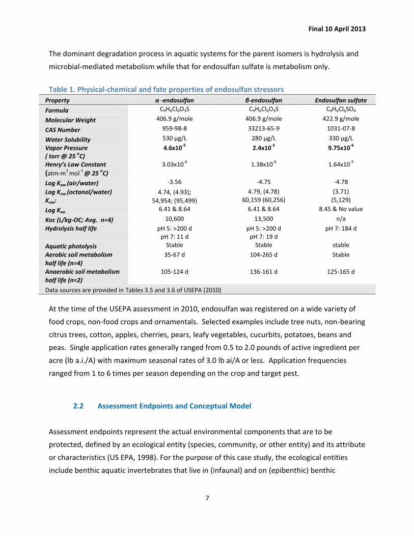
Relevant physical-chemical and environmental fate properties of the endosulfan stressors of

concern are summarized in Table 1. Based on its vapor pressure, endosulfan is considered a

semi-volatile chemical and as a result, volatilization and atmospheric transport are potential

environmental exposure pathways of concern. The α and β isomers show high hydrophobicity

(log KOW ~ 4.7), while endosulfan sulfate is less hydrophobic (log KOW 3.7). The KOC for α and β

isomers are 10,600 and 13,500 L/kg-OC , respectively. All three chemical components of the

stressor are therefore expected to partition extensively to organic phases of aquatic

ecosystems (sediments, dissolved and particulate organic carbon, and lipid phases of biota).

2 A complete discussion of the degradates of interest for endosulfan is found in Section 3.2.1 of USEPA (2010).

Final 10 April 2013

7

The dominant degradation process in aquatic systems for the parent isomers is hydrolysis and

microbial-mediated metabolism while that for endosulfan sulfate is metabolism only.

Table 1. Physical-chemical and fate properties of endosulfan stressors

Property α -endosulfan β-endosulfan Endosulfan sulfate

Formula C9H6Cl6O3S C9H6Cl6O3S C9H6Cl6SO4

Molecular Weight 406.9 g/mole 406.9 g/mole 422.9 g/mole

CAS Number 959-98-8 33213-65-9 1031-07-8

Water Solubility 530 µg/L 280 µg/L 330 µg/L

Vapor Pressure ( torr @ 25

oC)

4.6x10-5

2.4x10-5

9.75x10-6

Henry’s Law Constant (atm-m

3 mol

-1 @ 25

oC)

3.03x10-6

1.38x10-6

1.64x10-5

Log Kaw (air/water) -3.56 -4.75 -4.78

Log Kow (octanol/water)

Kow:

4.74, (4.93); 54,954; (95,499)

4.79, (4.78) 60,159 (60,256)

(3.71) (5,129)

Log Koa 6.41 & 8.64 6.41 & 8.64 8.45 & No value

Koc (L/kg-OC; Avg. n=4) 10,600 13,500 n/a

Hydrolysis half life pH 5: >200 d pH 7: 11 d

pH 5: >200 d pH 7: 19 d

pH 7: 184 d

Aquatic photolysis Stable Stable stable

Aerobic soil metabolism

half life (n=4)

35-67 d 104-265 d Stable

Anaerobic soil metabolism

half life (n=2)

105-124 d 136-161 d 125-165 d

Data sources are provided in Tables 3.5 and 3.6 of USEPA (2010)

At the time of the USEPA assessment in 2010, endosulfan was registered on a wide variety of

food crops, non-food crops and ornamentals. Selected examples include tree nuts, non-bearing

citrus trees, cotton, apples, cherries, pears, leafy vegetables, cucurbits, potatoes, beans and

peas. Single application rates generally ranged from 0.5 to 2.0 pounds of active ingredient per

acre (lb a.i./A) with maximum seasonal rates of 3.0 lb ai/A or less. Application frequencies

ranged from 1 to 6 times per season depending on the crop and target pest.

2.2 Assessment Endpoints and Conceptual Model

Assessment endpoints represent the actual environmental components that are to be

protected, defined by an ecological entity (species, community, or other entity) and its attribute

or characteristics (US EPA, 1998). For the purpose of this case study, the ecological entities

include benthic aquatic invertebrates that live in (infaunal) and on (epibenthic) benthic

Final 10 April 2013

8

sediments in freshwater and saltwater ecosystems. The attributes considered for protection of

benthic aquatic invertebrates include survival, growth, development and reproduction of

benthic invertebrates. These assessment endpoints were selected because of their relationship

to population level effects. Measures of ecological effects for benthic invertebrates include

LC50/EC50 and NOAEC values based on endpoints of survival, growth (dry weight, length),

development (development rate) and reproduction (fecundity, emergence rate).

A conceptual model provides a written and visual description of the predicted relationships

between the stressor (total endosulfan), potential routes of exposure, and the predicted effects

for the assessment endpoint. The overall conceptual model used in the 2010 endosulfan

ecological risk assessment is shown in Figure 2. Since benthic invertebrates are the focus of this

case study, a more detailed discussion of stressor sources, exposure routes and predicted

effects on benthic invertebrates is provided below.

Routes of entry for endosulfans to aquatic ecosystems include: 1) direct deposition of pesticide

droplets from spray drift, 2) inflow of pesticide contaminated runoff, 3) influx of erosion of

contaminated soil, 4) leaching to groundwater and subsequent input (likely limited to highly

porous soils with low organic content), and 5) wet and dry deposition from atmospherically-

transported chemical. Once in the waterbody, endosulfans are expected to predominately sorb

onto suspended sediment and other organic matter present in the water column with

subsequent deposition onto bed sediments via sedimentation. Benthic aquatic invertebrates

may be exposed to endosulfans primarily through respiration of interstitial (pore) water,

respiration of overlying water, ingestion of sediment particles and aquatic prey, and dermal

absorption.

Final 10 April 2013

9

Figure 2. Conceptual model for agricultural uses of endosulfan.

2.3 Analysis Plan

The primary method used to assess ecological risk by OPP is the risk quotient (RQ). The RQ is

the result of comparing measures of exposure to measures of effect:

RQ = exposure concentration / effect concentration

Risk quotients are determined separately for acute (short-term) and chronic (long-term)

exposures and associated effect concentrations. For endosulfan, multiple methods were used

for estimating the exposure concentration for benthic invertebrates. These include:

Modeled concentrations in sediment pore water,

Modeled concentrations in bulk sediment (normalized for OC), and

Stressor Application of Endosulfan to an Agricultural Field

Source/

Transport

Pathways

Direct

Deposition

Spray

Drift

Runoff /

Erosion

Leaching

(infiltration /

Percolation)

Source/

Exposure

Media

Terrestrial Food

Residues (foliage,

fruits, insects)

Receiving

Water Body/

Sediment

Groundwater

Irrigation

water

on crops

Exposure

RouteIngestion

Absorption

& Root Uptake

Uptake via Gill, Skin, &

Sediment Ingestion

ReceptorsTerrestrial Vertebrates

Birds, Mammals, Reptiles,

Terrestrial Phase Amphibians

Aquatic

PlantsAquatic Invertebrates

and Vertebrates

Attribute

Changes

Terrestrial Vertebrates

Reduced survival

Reduced growth

Reduced reproduction

Plant Population

Reduced

population growth

Aquatic Vertebrates

and Invertebrates

Reduced survival

Reduced growth

Reduced reproduction

Trophic TransferPrey Ingestion

Prey I

ngestio

n

Volatilization /

Wind Suspension

Regional/Long-Range

Transport

Atmospheric

Deposition

Inhalation

Terrestrial

Plants

Dermal

Uptake

Soil

Air

Final 10 April 2013

10

Monitored concentrations in bulk sediment.

Since the 2010 endosulfan ecological risk assessment was a “screening-level” assessment,

“high-end” estimates of exposure were developed for comparing to effect concentrations. For

modeled concentrations, an estimated environmental concentration (EEC) was developed for

pore water and bulk sediment. The EEC has two components: a return frequency and an

averaging period. For OPP screening-level assessments, a 1-in-10 year return frequency is

selected from a 30-year time series of daily concentrations of pesticides in surface water, pore

water and bulk sediment. The averaging period (i.e., the time period over which the pesticide

concentrations are averaged for comparing with the effect concentration) varies depending on

the taxa and type of risk being evaluated (acute vs. chronic). For aquatic invertebrates, acute

risk is determined from daily (peak) concentrations while chronic risk is determined from 21-d

moving average concentrations that correspond to the aforementioned return frequency. For

monitored concentrations, data are usually much less abundant compared to model-derived

estimates and therefore, upper bound (e.g., maximum) values are typically selected.

Measures of effect (i.e., the denominator of the RQ) also vary depending on the type of risk

being evaluated (acute vs. chronic). For acute risks to pelagic invertebrates, toxicity values such

as the 48-h or 96-h LC50 (lethal concentration to 50% of test organisms) or the 48-h or 96-h EC50

(effect concentration to 50% of test organisms) are typically selected. For chronic risk to

invertebrates, the NOAEC (No Observed Adverse Effect Concentration) is selected from a

standard life cycle toxicity test (e.g., 21 days for Daphnia magna; 28 days for Americamysis

bahia). For deterministic risk assessments, these acute and chronic effect endpoints are

selected from the most sensitive species for which valid toxicity data are available.

With sediment toxicity tests of benthic invertebrates, standard exposure durations do not

conform to those used in water column tests of pelagic invertebrates. Typically, subchronic

sediment toxicity tests required by OPP include 10-day subchronic exposures to selected

species (e.g., Chironomus dilutus, Hyalella azteca, Leptocheirus plumulosus) in which effects on

survival and growth are measured. Chronic sediment toxicity tests include 28 to 65-day life

cycle exposures in which effects on survival, growth, reproduction and development are

measured. As a matter of current practice3, measures of chronic risk are determined from the

3 Formal guidance on selecting toxicity endpoints and EECs for benthic invertebrates risk assessment are currently

under development in OPP.

Final 10 April 2013

11

pore water and/or bulk sediment NOAEC for the most sensitive species available from

subchronic and chronic sediment toxicity testing. This NOAEC is used to compare with the 21-d

EEC for calculating the chronic sediment RQ. For estimating acute risks to benthic

invertebrates, current practice involves selecting the most sensitive LC50 or EC50 available from

the water column acute toxicity tests for aquatic invertebrates (Table 2).

Table 2. Assessment endpoints, measures of effect, and measures of exposure used for assessing risk to pelagic and benthic aquatic invertebrates

Taxa Assessment Endpoint Type of RQ

Measures of Ecological Effect

1 Measures of Exposure2

Freshwater invertebrates (pelagic)

Survival Acute Acute (48-96 h) LC50 or EC50

Peak water column EEC

Survival, growth, reproduction and development

Chronic Chronic (21-d) NOAEC 21-day average water column EEC

Freshwater invertebrates (benthic)

Survival Acute Acute (48-96 h) LC50 or EC50 (from water column test)

Peak EEC for pore water


Chronic Subchronic (10-d) or chronic (28-65-d) NOAEC

21-day average EEC for porewater and/or bulk sediment

Estuarine/marine invertebrates (pelagic)

Survival Acute Acute (48-96 h) LC50 or EC50

Peak water column EEC


Chronic Chronic (28-d) NOAEC 21-day average water column EEC

Estuarine/marine invertebrates (benthic)

Survival Acute Acute (48-96 h) LC50 or EC50 (from water column test)

Peak EEC for pore water


Chronic Subchronic (10-d) or chronic (28-d) NOAEC

21-day average EEC for porewater and/or bulk sediment

1 Toxicity test durations in parentheses reflect those from typical test species

2 Based on a 1-in-10-year return frequency for model-derived exposure estimates. For monitored exposure

concentrations, upper bound (e.g., maximum) concentrations are typically selected.

Following the calculation of the applicable RQs, comparisons are then made to the established “Level of Concern” (LOC). If the RQ values exceed the LOC, risk is presumed. For acute risks to non-listed4 aquatic invertebrates, an LOC of 0.5 is used while for chronic risks, an LOC of 1.0 is used. A more detailed discussion of the basis of the LOCs is found in USEPA (2004).

4 The term “non-listed” refers to species that are not considered “threatened or endangered” under the US

Endangered Species Act (ESA). For ESA listed species, different LOC values are used.

Final 10 April 2013

12

3. EXPOSURE ASSESSMENT Two different methods were used for assessing exposure of benthic invertebrates to

endosulfans. The first method used modeled chemical concentrations in pore water and bulk

sediment. The second method used measured endosulfan concentrations in sediment. Each of

these methods is summarized below.

3.1 Modeled Sediment Concentrations

The USEPA Pesticide Root Zone Model (PRZM) and the Exposure Analysis Modeling System

(EXAMS) models were used to estimate concentrations of endosulfans in bulk sediment and in

pore water. The PRZM model is simulation model that calculates the fate of a pesticide in

treated fields on a day-to-day basis. It considers how factors such as climatic conditions,

evapotranspiration of plants, soil physicochemical and hydrological characteristics, crop-specific

management practices, pesticide applications and pesticide fate parameters affect the degree

to which a pesticide is taken up in the plant, leaches through the soil, volatilizes into the

atmosphere, and is transported off site via runoff and soil erosion. Simulations are run with

over 30 years of climate data for crop scenarios that vary by crop and region of the country.

Daily estimates of pesticide runoff and erosion from PRZM are then used as input to the EXAMS

model, along with estimates of pesticide spray drift. The EXAMS model is parameterized for a

“standard agricultural pond” 20 million liter pond of approximately 2 meters depth that is

surrounded by an agricultural field. The EXAMS model accounts for volatilization, sorption,

hydrolysis, biodegradation, and photolysis of the pesticide in the aquatic environment. The

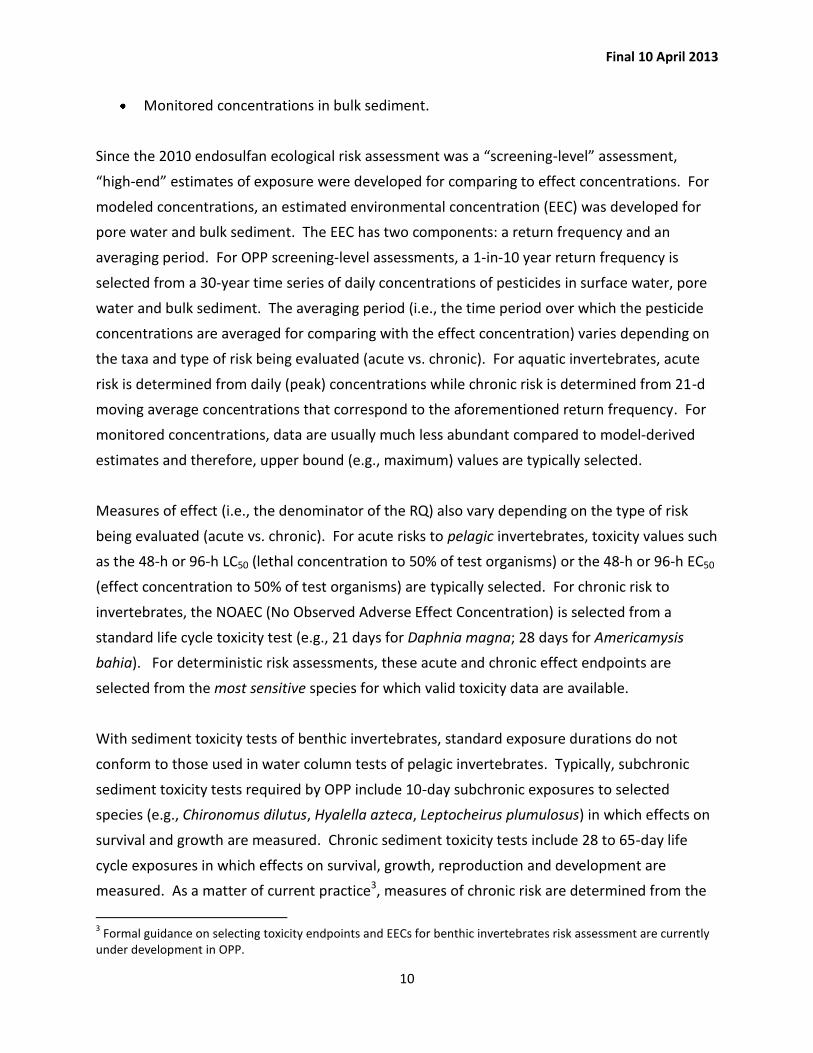
standard pond is represented by two compartments (water column and sediment layers). A

conceptual representation is shown in Figure 3. Bioavailability of a nonionic organic pesticide

like endosulfan is modeled in water based on equilibrium partitioning between the freely

dissolved, DOC and POC-sorbed phases. Sediments are typically assumed to contain 4% organic

carbon.

The end result of the PRZM and EXAMS model simulations is a 30-year time series of daily

pesticide concentrations in overlying water, pore water and bulk sediment for each crop

exposure scenario. Based on these 30-year time series, EECs were calculated for specified

averaging periods (peak for acute exposures and 21-d for chronic exposures) that correspond to

Final 10 April 2013

13

a 1-in-10 year return frequency. Predicted EECs for endosulfans in surface water, pore water

and bulk sediment (dry weight) are shown in Figure 4 for selected crop scenarios.

Figure 3. Conceptual model of OPP Standard Pond Scenario for Depicting Pesticide Transport

Arrows represent movement of pesticide mass from one phase (i.e., sorbed or aqueous) or compartment to another. In this figure, Paqeous=aqueous mass of pesticide; Psorbed= sorbed mass of pesticide; and Pgas= gaseous mass of pesticide. Grey arrows are pathways not routinely simulated.

Benthic

Area

Water Column

Psorbed

Paqueous

Ru

noff

Sp

ray D

rift

We

t De

po

sitio

n

(rain

)

Instant Equilibrium

Instant Equilibrium

Vo

latiliz

atio

n

Pgas

Re

su

sp

en

sio

n

Aq

ue

ous M

ixin

g

Paqeous

(pore water)

Se

ttling

Paqueous

Ero

sio

n +

Se

ttling

(PR

BE

N)

Psorbed

Psorbed

Dry

dep

ositio

n

Ero

sio

n

These processes addressed

as one lumped mass transfer coefficient (Ω)

Bu

rial

Bu

rial

Final 10 April 2013

14

Figure 4. Predicted EECs of total endosulfan in pore water and sediment.

3.2 Monitored Sediment Concentrations

An extensive array of monitoring data was available for endosulfans measured in sediments

across the U.S. The three main data sources are included in this case study:

The US Geological Survey the North American Water Quality Assessment program

(NAWQA) database5;

The National Sediment Quality Survey6 (NSQS) database; and

The South Florida Water Management District (SFWMD)7 database (1992-2008).

5

NAWQA data was obtained on January 17, 2008: URL: http://infotrek.er.usgs.gov/traverse/f?p=NAWQA:HOME:3748645897450568 6 http://epa.gov/waterscience/cs/library/nsidbase.html

7 Detailed maps of station locations can be found at:

http://my.sfwmd.gov/portal/page/portal/pg_grp_sfwmd_era/pg_sfwmd_era_hydrometmonlocations

0.0

0.5

1.0

1.5

2.0

2.5

3.0

3.5

Citru

s (F

L)

Co

tto

n (S

. TX

)

Co

tto

n (C

A)

To

mato

(P

A)

To

mato

(C

A)

Dry

Bean

s (

IL)

Dry

Bean

s (

WA

)

Cucurb

its (S

. T

X)

Cucurb

its (C

A)

Po

tato

(M

E)

Po

tato

(W

A)

Fru

its (M

I)

Fru

its (W

A)

To

bacco

(N

C)

Lettuce (

CA

)

Eg

gp

lan

t (C

A)

Po

re W

ate

r E

EC

s (

pp

b)

Crop Scenario

Peak EEC

21-day EEC

0

200

400

600

800

1000

1200

1400

1600

Citru

s (F

L)

Co

tto

n (S

. TX

)

Co

tto

n (C

A)

To

mato

(P

A)

To

mato

(C

A)

Dry

Bean

s (

IL)

Dry

Bean

s (

WA

)

Cucurb

its (S

. T

X)

Cucurb

its (C

A)

Po

tato

(M

E)

Po

tato

(W

A)

Fru

its (M

I)

Fru

its (W

A)

To

bacco

(N

C)

Lettuce (

CA

)

Eg

gp

lan

t (C

A)Sed

imen

t E

EC

s (

ug

/kg

dw

)

Crop Scenario

Peak EEC

21-day

EEC

http://infotrek.er.usgs.gov/traverse/f?p=NAWQA:HOME:3748645897450568

http://epa.gov/waterscience/cs/library/nsidbase.html

http://my.sfwmd.gov/portal/page/portal/pg_grp_sfwmd_era/pg_sfwmd_era_hydrometmonlocations

Final 10 April 2013

15

A brief summary of each of these databases is provided below. Additional details are found in

USEPA (2010).

NAWQA Database. The NAWQA monitoring program represents a national scale network of

numerous sites throughout the US that is intended for evaluation of broad spatial and temporal

trends in contaminant concentrations. Sampling in regions alternate among different years.

With respect to endosulfan in sediments, data were available from 1992-2007 and only the α

endosulfan isomer was measured (not the β isomer or endosulfan sulfate degradate).

NSQI Database. The NSQI database reflects a compilation of sediment contaminant information

from a wide variety of sources in the US, many of which are monitoring programs established at

the State and local levels. For endosulfan, information was available from 1990 to 1998 and

analyses were conducted on the parent isomers but not the endosulfan sulfate degradate. The

spatial distribution of detections and non-detect from the NAWQA and NSQI databases for

endosulfan is shown in Figure 5. A summary of the frequency of detection of endosulfan

isomers and overall maxima is shown in Table 3 and the overall distribution of detected

endosulfans (α + β) is provided in Figure 6.

Figure 5. A map showing spatial distribution of endosulfans monitored in sediments from NAWQA (alpha endosulfan) and the NSQI (alpha & beta)

Final 10 April 2013

16

Table 3. Detection frequency and maximum sediment concentrations for endosulfan isomers

Figure 6. Frequency distribution of endosulfan detections (alpha + beta) in U.S. sediments from the NAWQA and NSQI databases

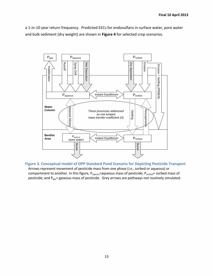
SFWMD Database. An extensive water quality monitoring network was available from the

South Florida Water Management District’s (SFWMD) that included sampling for pesticides in

surface water and benthic sediment from numerous sites in South Florida. The data described

herein represent endosulfans measured in sediment twice a year from 1992 – 2008 as reported

in the SFWMD DBHYDRO database.8 Data were reported for the α and β isomers and

endosulfan sulfate. A map of the station locations is shown in Figure 7. Results for each of the

SFWMD stations over this time period are provided in Table 4 and those for the most

contaminated station (S-178) are provided in Figure 8. An important limitation with these data

is the lack of available information on the organic carbon content in sediment.

8

Download date: Feb 6, 2009. Available at: https://my.sfwmd.gov/portal/page/portal/pg_grp_sfwmd_era/pg_sfwmd_era_dbhydrobrowser

74%

4%

6%

6%10%

Endosulfan (alpha + beta)

<0.11 ug/kg dw >0.0.11-0.5 ug/kg dw >0.5-5.5 ug/kg dw

>5.5-55 ug/kg dw > 55 ug/kg dw

Data Source Monitoring Period

Number of Samples

Maximum Reported

Concentration (μg/Kg)

Detects No detects Total Detects % Alpha Beta SO4

NAWQA 1992- 2001 & 2007 24 1,249 1,273 2% 8.8 ND ND

NSQI 1990-1998 507 8,218 8,725 6% 430 192 ND

ND= Not determined

https://my.sfwmd.gov/portal/page/portal/pg_grp_sfwmd_era/pg_sfwmd_era_dbhydrobrowser

Final 10 April 2013

17

Figure 7. Sampling Locations of SFWMD water quality monitoring stations associated with the Everglades National Park (ENP) and Florida Bay (FLBAY) project areas

Table 4. Concentrations of endosulfans in sediment at SFWMD sampling sites with at least one reported detection (data source: SFWMD)

Station ID No.

Samples No. Detects Detection

Frequency (1)

Total Endosulfans (μg/kg dw)

Min. Average (2)

Max.

C-111 Canal System

S177 32 10 31% bdl 2.9 55

S178 33 23 70% bdl 39.4 152

S18C 35 1 3% nd nd 6.3

Subtotal 100 34 34%

L-31 Canal System

S331 23 1 4% nd nd 4.1

Other Stations

C25S99 32 1 3% nd nd 1

G354C 1 1 100% nd nd 2.6

G393B 1 1 100% nd nd 5

G600 1 1 100% nd nd 1.3

Final 10 April 2013

18

Station ID No.

Samples No. Detects Detection

Frequency (1)

Total Endosulfans (μg/kg dw)

Min. Average (2)

Max.

L3BRS 1 1 100% nd nd 0.9

S5A 32 1 3% nd nd 6.5

S6 27 1 4% nd nd 111

S79 31 1 3% nd nd 9.2

S80 33 1 3% nd nd 6.6

Subtotal 190 9 4.7%

(1) Frequencies of detection of 0.1 (10%) or higher are highlighted in bold. (2) Averages in μg/L calculated assuming that concentrations reported as being below the limit of analytical detection (bdl) contained 0 μg/L endosulfans. (3) Total endosulfans = sum of alpha, beta and endosulfan sulfate analytes. bdl = below method detection limit (typically from 0.001-0.02 ppb). nd = not determined.

Figure 8. Annual Average and maximum concentrations of total endosulfans in sediment from the C-111 canal stations with at least one detection (1992-2008; source: SFWMD, error bars = 1 std. dev.)

4. EFFECTS ASSESSMENT

4.1 Sediment Toxicity Data The USEPA’s 2010 ecological risk assessment for benthic invertebrates was based on registrant-

submitted sediment toxicity data on the primary degradate, endosulfan sulfate. From an

environmental fate perspective, endosulfan sulfate is the dominant form of endosulfan

expected in sediments due to its higher persistence relative to the parent isomers. From a

toxicological perspective, past studies indicate similar toxicity of endosulfan sulfate and the

parent isomers (USEPA, 2007). For freshwater benthic invertebrates, two studies were

submitted on the toxicity of endosulfan sulfate to the freshwater midge, Chironomus dilutus.

The first study involved a 10-day subchronic exposure to sediments spiked with endosulfan

0

20

40

60

80

100

120

140

160

1992 1994 1996 1998 2000 2002 2004 2006 2008

Sampling Year

To

tal E

nd

osu

lfan

s (

ug

/kg

dw

) Annual Mean

Annual Max

Final 10 April 2013

19

sulfate (MRID 46382605; Table 5). The 10-d EC50 values for survival and growth determined

from this study are 10.0 and 6.4 μg a.i./L-pw, respectively. The 10-d NOAEC for midge survival

is 0.63 ug a.i./L-pw which is about 4X more sensitive than the NOAEC based on growth (NOAEC

= 2.7 μg a.i./L-pw). The 10-d NOAECs for survival and growth in bulk sediment are 0.13 and

0.56 mg a.i./kg-dw, respectively. When normalized to 100% organic carbon, the 10-d NOAECs

for survival and growth are 4.2 and 18.1 mg a.i./kg-OC, respectively. Examination of the

statistical comparisons indicated hypothesis testing of survival and growth endpoints has

similar statistical power (e.g., MSD= 15% and 23%, respectively).

The second sediment toxicity study with C. dilutus consisted of a 50-d exposure to endosulfan

sulfate from which effects on survival, growth and reproduction were assessed (MRID

47318101). A NOAEC of 0.35 μg a.i./L-pw and 0.17 mg/kg dw are derived from this study based

on survival (20-d) and emergence (50-d). The corresponding LOAEC values are 1.2 μg a.i./L-pw

and 0.4 mg/kg-dw). Statistically significant adverse effects on growth (20-d dry weight) and

reproduction (# eggs/female, % hatch) were not observed at the highest test concentration (1.2

μg a.i./L-pw and 0.4 mg/kg-dw).

Two toxicity studies were also available on the effects of endosulfan sulfate on the estuarine

amphipod, Leptocheirus plumulosus via sediment exposure (Table 5). In the first study (MRID

46382606), a 10-day subchronic test was conducted which produced a NOAEC and LOAEC of 27

and 45 μg a.i./L-pw, respectively, based on mortality. Effects on growth were not determined.

In a chronic 28-day test, the most sensitive NOAEC and LOAEC were determined as 1.58 and 4.0

μg a.i./L-pw, respectively based on growth and reproduction (MRID 46929001).

Table 5. Toxicity of Endosulfan Sulfate to Benthic Invertebrates Via Sediment Exposure.

Test Species Exposure Duration Endpoint

(a)

Pore Water (μg ai/L)

Bulk Sediment (mg ai/kg dw)

Sediment OC Normalized (mg a.i./kg-OC)

Freshwater midge, Chironomus dilutus (3.1% TOC, MRID 46382605)

10-d

Survival: EC50 NOAEC LOAEC

10.0 0.63 1.7

3.1 0.13 0.25

100 4.2 80.6

Growth: EC50 NOAEC LOAEC

6.4 2.7 3.8

1.9 0.56 1.2

61.3 18.1 38.7

Final 10 April 2013

20

Test Species Exposure Duration Endpoint

(a)

Pore Water (μg ai/L)

Bulk Sediment (mg ai/kg dw)

Sediment OC Normalized (mg a.i./kg-OC)

Freshwater midge, Chironomus dilutus (9.3% TOC; MRID 47318101)

50-d

Survival & Emergence: NOAEC LOAEC

0.35 1.2

0.17 0.4

1.8 4.3

Growth: NOAEC LOAEC

1.2 >1.2

0.4 >0.4

4.3 >4.3

Reproduction: NOAEC LOAEC

1.2 >1.2

0.4 >0.4

4.3 >4.3

Estuarine Amphipod, Leptocheirus plumulosus (1.6% TOC; MRID 46382606)

10-d


74 27 45

2.3 0.86 1.6

144 53.8 100

Estuarine Amphipod, Leptocheirus plumulosus (4.7% TOC MRID 46929001)

28-d


>4.0 4.0 >4.0

>1.2 1.2 >1.2

>25.5 25.5 >25.5

Growth: EC50 NOAEC LOAEC

>4.0 1.58 4.0

>1.2 0.48 1.2

>25.5 10.2 25.5

Reproduction: NOAEC LOAEC

1.58 4.0

0.48 1.2

10.2 25.5

(a)The lowest NOAEC values within freshwater and saltwater taxa are presented in bold.

4.2 Water Column Toxicity Data Information from water column toxicity tests of invertebrate species can also provide useful

information for assessing risks to benthic invertebrates. Specifically, toxicity to aquatic

invertebrates can be assumed equivalent between exposures via the water column and pore

water. Under the assumption of equilibrium partitioning (EqP) of a non-ionic organic chemical

among the pore water and sediment organic carbon phases, risk can then be assessed by

comparing water column toxicity values to predicted or measured concentrations in pore

water. Although this approach was not used in the 2010 endosulfan ecological risk assessment

due to the availability of sediment toxicity data, the EqP approach has been historically used by

OPP for benthic invertebrate risk assessment in the absence of sediment toxicity data. It is also

the basis of USEPA sediment quality benchmarks (USEPA 2002). With endosulfan, the breadth

of water column-based toxicity data available for invertebrates provides an opportunity to

Final 10 April 2013

21

compare the results of the EqP-based approach with those obtained from use of the set of

whole sediment toxicity tests described previously. Therefore, a brief description of the

applicable endosulfan water column toxicity tests for aquatic invertebrates is provided below.

The most sensitive freshwater aquatic invertebrate for which registrant-submitted acute

toxicity data were available at the time of the 2010 risk assessment was for the stonefly,

Pteronarcys californica, with a 96-h LC50 of 2.3 μg a.i./L (MRID 40094602). However, much

more information on the acute toxicity of endosulfan was available in the open literature.

Specifically, applicable acute LC/EC50 values USEPA’s ECOTOX database were identified and

reviewed for their acceptability for pesticide risk assessment. These acute toxicity data range in

exposure durations from 0.5 to 4 days and are shown in Figure 9. If values for multiple

durations were available from a single test, then only the value from longest duration (up to 48-

96 hours, depending on species) was used to make the comparison with the lowest registrant-

submitted toxicity reference value of 2.3 μg a.i./L. There were 89 LC/EC50 values from 37 open

literature studies representing 42 freshwater invertebrate species. Twenty-one of these values

were below the registrant-submitted 2.3 μg a.i./L toxicity reference value (shown in red in

Figure 9). A detailed review of these data for their suitability in USEPA pesticide risk assessment

indicated the most acutely sensitive species for which acceptable data were available was for

the mayfly, Jappa kutera (Leonard et al., 2001). Specifically, Leonard et al. (2001) compared the

sensitivity of different forms of endosulfan to the freshwater mayfly, J. kutera. These forms

included α and β endosulfan, a technical grade mixture (7:3 ratio of α and β), and endosulfan

sulfate. The 96-h LC50 values were 0.7, 2.3, 1.8 and 1.2 μg a.i./L, respectively. The lowest of

these values (0.7 μg a.i./L for α endosulfan) was selected for use in the 2010 risk assessment

for freshwater (pelagic) invertebrates (Table 6). This 96-h LC50 value is about an order of

magnitude lower than the 10-d LC50 value of 10 μg a.i./L-pw available for the midge, C. dilutus,

despite the 2-fold longer duration of the midge study.

Final 10 April 2013

22

Figure 9. Freshwater invertebrate endosulfan acute toxicity data from ECOTOX (USEPA 2010). Red line denotes the lowest available LC50 value from registrant-submitted data (2.3 μg a.i./L)

Table 6. Acute and chronic toxicity reference values used for assessing endosulfan risk to water column invertebrates (USEPA 2010)

Species

Most Sensitive Toxicity Value Considered Acceptable for Risk Assessment (μg a.i./L)

Effects Reference/Acceptability

Freshwater Invertebrates

Mayfly (Jappa kutera) 96-h LC50 = 0.7 Mortality

Leonard, et al. 2001; (ECOTOX 62479)/

Chronic NOAEC = 0.011 Not Available Estimated (1)

Estuarine/Marine Invertebrates

Pink shrimp (Penaeus dourarum)

96-h LC50 = 0.04 Mortality MRID 5005824 Chronic NOAEC = 0.013 Not Available Estimated

(2)

(1) The daphnid (Daphnia magna) acute-to-chronic ratio (ACR = 61.5) was used to estimate a freshwater mayfly

chronic toxicity value because it is the most acutely sensitive freshwater invertebrate species and no chronic toxicity data are available for it. (2)

The mysid shrimp (Americamysis bahia) acute-to-chronic ratio (ACR = 3.1) was used to estimate pink shrimp chronic toxicity value because it is the most acutely sensitive saltwater invertebrate species and no chronic toxicity data are available for it.

A chronic NOAEC of 0.011 μg a.i./L was estimated for the mayfly, J. kutera, by dividing its acute

LC50 of 0.7 μg a.i./L by an endosulfan-specific acute to chronic ratio of 61.5 derived for D.

magna. Although measured chronic toxicity data were available for D. magna (21-d NOAEC =

2.7 μg a.i./L), it is higher than the acute LC50 value for J. kutera (0.7 μg a.i./L ) which indicates it

is not among the more sensitive aquatic invertebrates to endosulfan.

Endosulfan: Freshwater Invertebrate LC50s

n = 89

0.00

0.10

0.20

0.30

0.40

0.50

0.60

0.70

0.80

0.90

1.00

0.001 0.01 0.1 1 10 100 1000 10000 100000

LC50 (ug/L)

Pro

ba

bili

ty R

ank

Final 10 April 2013

23

For saltwater invertebrates, acute toxicity values were available from registrant-submitted

studies for four species that had 96-h LC50 values ranging from 0.04 to 790 μg a.i./L. The most

sensitive 96-h LC50 value of 0.04 μg a.i./L (MRID 5005824) for pink shrimp (Penaeus dourarum)

was considered acceptable for estimating acute risks to estuarine/marine invertebrates. No

other acceptable acute toxicity values from the open literature were found to be lower than

this value for pink shrimp at the time of the 2010 risk assessment. A chronic NOAEC of 0.013 μg

a.i./L was estimated for the pink shrimp (P. dourarum) by dividing the acute LC50 of 0.04 μg

a.i./L by an endosulfan-specific acute to chronic ratio of 3.1 derived for Americamysis bahia.

Although measured chronic toxicity data were available for A. bahia (28-d NOAEC = 0.14 μg

a.i./L), it is higher than the acute LC50 value for P. dourarum (0.04 μg a.i./L ) which indicates it is

not among the more sensitive aquatic invertebrates to endosulfan.

5. RISK CHARACTERIZATION In the USEPA 2010 assessment, risk to benthic invertebrates was determined based on

comparisons of the EEC (described in Section 3) to the appropriate sediment toxicity endpoint

(Described in Section 4). For the purposes of this case study, risks are also estimated based on

comparisons of the EECs in pore water to the appropriate toxicity endpoints derived from water

column toxicity tests. Risks were also estimated based on monitored concentrations of

endosulfans in sediment. The results from each of these risk comparisons are summarized in

the following sections.

5.1 Predicted EECs vs. Sediment Toxicity Endpoints

With the predicted EECs, risk quotients (RQs) for benthic invertebrates were estimated based

on comparison with the sediment toxicity endpoints estimated in pore water and those

estimated on a sediment organic carbon basis. Specifically:

Pore water RQ = 21-d EEC (μg a.i./L-pw) NOAEC (μg a.i./L-pw)

Sediment RQ = 21-d EEC (mg a.i./kg-OC) NOAEC (mg a.i./kg-OC)

Final 10 April 2013

24

Chronic RQ values derived for selected endosulfan crop exposure scenarios are provided in

Table 7. These RQ values are based on modeled total endosulfan EECs in pore water compared

to lowest available chronic sediment NOAEC measured in pore water. The pore water-based

sediment RQs exceed the chronic risk LOC of 1.0 in 11 of the 16 crop scenarios modeled for

freshwater benthic invertebrates and 7 of the 16 crop scenarios modeled for estuarine/marine

benthic invertebrates. These results suggest that invertebrates are at risk of chronic effects on

survival and reproduction from prolonged exposure to endosulfans in sediment.

Table 7. Chronic Risk Quotients for Benthic Aquatic Invertebrates Based on Modeled EECs and Measured Sediment Toxicity in Pore Water

Crop Use Category

EEC Range Crop Scenario 21-day EEC (µg/L-p.w.)

RQ (fw)1 RQ (sw)

2

Citrus-nb Overall Maximum FL Citrus-nb

2.99 8.5 1.9

Cotton

High S. TX Cotton 1.76 5.0 1.1

Low CA Cotton 0.32 0.9 0.2

Tomato

High PA Tomato 2.57 7.3 1.6

Low CA Tomato 0.27 0.8 0.2

Beans & Peas (dry)

High IL Beans 2.66 7.6 1.7

Low WA Beans 0.28 0.8 0.2

Cucurbits

High S. TX Melon 1.73 5.0 1.1

Low CA Melon 0.42 1.2 0.3

Potatoes

High ME Potato 2.13 6.1 1.4

Low WA Potato 0.40 1.2 0.3

Fruits

High MI Cherry 1.63 4.7 1.0

Low WA Orchards 0.18 0.5 0.1

Lettuce n.a. CA Lettuce 1.18 3.4 0.7

Tobacco n.a. NC Tobacco 0.73 2.1 0.5

Eggplant Overall Minimum CA Eggplant

0.09 0.3 0.1

1 RQs based on the 50-d NOAEC of 0.35 μg/L porewater reported for survival and emergence of C. dilutus (MRID

473181-01) 2

RQs based on the 28-D NOAEC of 1.58 μg/L porewater reported for growth of L. plumulosus (MRID 469290-01) RQ values in bold and shaded exceed or meet the chronic risk LOC of 1.0.

Chronic RQ values expressed on the basis of sediment organic carbon are provided in Table 8.

The sediment OC-based RQs exceed the chronic risk LOC of 1.0 in 15 of the 16 crop scenarios

modeled for freshwater benthic invertebrates and 8 of the 16 crop scenarios modeled for

estuarine/marine benthic invertebrates. Furthermore, it is evident that the magnitude of the

chronic sediment OC-based RQ values is approximately a factor of 2 higher than the

corresponding pore water-based RQ values.

Final 10 April 2013

25

The higher RQ values on the basis of sediment OC appears to reflect differences between the

organic carbon partitioning assumed in modeling the sediment EECs compared to that which

actually occurred in the sediment toxicity test. Specifically, KOC values ranging from 10,600 to

13,500 L/kg-OC were used in the derivation of the pore water and sediment-based EECs using

the PRSM and EXAMS models. These KOC values are based on standard sorption/desorption

studies conducted using various soils of α and β endosulfan. By comparison, the “sediment ”

KOC values9 that correspond to the NOAECs from the sediment toxicity tests in Table 5 range

from approximately 2,000 to 6,700 L/kg-OC. The lower “sediment” KOC values relative to those

measured from the soil-based sorption/desorption studies are consistent with the lower

hydrophobicity of endosulfan sulfate (log KOW =3.7) compared to the α and β isomers (log KOW =

4.7 and 4.8, respectively). It may also be possible that greater amounts of dissolved endosulfan

sulfate are present in pore water of the sediment toxicity tests due to sorption with DOC which

may result in lower sediment KOC values. However, the log KOW of endosulfan sulfate (3.7)

suggests that the concentration of DOC in pore water would have to be relatively high in order

to substantially reduce the freely dissolved concentrations in pore water. Differences in the

sorptive capacity of organic carbon underlying the soil- and sediment-based KOC values may also

be a factor that contributes to the observed differences in KOC values. Thus, it appears from this

case study that evaluating risks to benthic organisms on the basis of both porewater and

sediment concentrations is beneficial to the risk assessment process because different sources

and levels of uncertainty may exist among predicted (or measured) pesticide concentrations in

porewater vs. bulk sediment.

Table 8. Chronic Risk Quotients for Benthic Aquatic Invertebrates Based on Modeled EECs and Measured Sediment Toxicity Normalized to Organic Carbon

Crop Exposure Scenario

EEC Range Crop Scenario

21-day EEC (mg/kg-OC)

RQ (fw)1 RQ (sw)

2

Citrus-nb Overall Maximum FL Citrus-nb 35.6 19.5 3.5

Cotton



Tomato



Beans & Peas (dry)



Cucurbits


Low CA Melon 5.3 2.9 0.5

Potatoes High ME Potato 25.3 13.8 2.5

9 These sediment Koc values were determined by dividing each sediment OC normalized NOAEC (ug/kg-oc) by its

corresponding porewater NOAEC (ug/L).

Final 10 April 2013

26

Crop Exposure Scenario

EEC Range Crop Scenario

21-day EEC (mg/kg-OC)

RQ (fw)1 RQ (sw)

2


Fruits





Eggplant Overall Minimum CA Eggplant 1.1 0.6 0.1

1 RQs based on the 50-d NOAEC of 1.83 mg/kg-OC reported for survival & emergence of C. dilutus (MRID

47318101) 2

RQs based on the 28-D NOAEC of 10.2 mg/kg-OC reported for growth & reproduction of L. plumulosus (MRID 46929001) Bold and shaded RQs exceed the acute risk to non-listed species LOC of 0.5.

5.2 Monitored EECs vs. Sediment Toxicity Endpoints Data on concentrations of endosulfans in sediments (µg/kg dry wt) were summarized earlier in

Section 3.2. These data sets included two that were national in scope (NSQI, NAWQA) and one

that focused on the South Florida region. Since porewater concentrations were not available

from field monitoring surveys, evaluation of these data in relation to toxicity to benthic

invertebrates was conducted on a sediment basis. Ideally, the fraction of organic carbon would

be known from the monitored sediment samples, and the sediment NOAEC could be adjusted

directly to match this OC value. However, such data were not readily available at the time of

the 2010 risk assessment. Therefore, comparisons of the maximum measured concentration of

endosulfans in sediment were made to the NOAEC adjusted to reflect low (2%), moderate (5%)

and high (10%) organic carbon content of sediments. Specifically, the NOAEC value of 0.17

mg/kg dw for the most sensitive invertebrate (C. dilutus, MRID 47318101) was adjusted to

reflect different fractions of organic carbon assumed in sediment (2%, 5% and 10%).

Results from this comparison (Table 9) indicate that maximum concentrations reported by the

NSQI and SFWMD studies approach or exceed the freshwater NOAEC for C. dilutus as adjusted

to all three values of sediment organic carbon. These results suggest that concentrations of

endosulfans in monitored sediments can reach levels that would be of concern for the

protection of freshwater benthic invertebrates for sediments that span a reasonably wide range

of total organic carbon. In contrast, concentrations of α endosulfan reported by the NAWQA

program are much lower and do not exceed any of the OC-adjusted NOAEC values. The

NAWQA program is much broader in spatial scale and is designed to evaluate long-term trends

in chemical concentrations rather than targeting particular sites or time periods that may be

Final 10 April 2013

27

particularly vulnerable to pesticide runoff. That program also measured only α endosulfan

which likely substantially under represents the concentration of total endosulfans in sediment.

Table 9. Comparison of Maximum Concentrations of Endosulfans Reported in U.S. Sediments with the Organic Carbon-Adjusted NOAEC for Freshwater Invertebrates

Study1 Location Analyte

Max. Conc. (ug/kg dry wt)

RQ (Conc./NOAEC)

2

2% OC 5% OC 10% OC

NAWQA USA α- isomer 8.8 0.2 0.1 0.0

NSQI USA α- isomer 430 11.8 4.7 2.4

SFWMD S. Florida α + β + SO4

152 4.2 1.7 0.8

1 Data sources are described in Section 3.2. Bold and shaded RQs exceed the chronic LOC of 1.0

2 RQ values determined by adjusting the NOAEC of 0.17 mg/kg dry wt (MRID 47318101; 9.3% OC) to reflect 2%, 5%

and 10% organic carbon in sediments (i.e., 0.037, 0.091, and 0.183 mg/kg dw, respectively).

5.3 Pore Water EECs vs. Water Column Toxicity Endpoints Although risks to benthic invertebrates were not estimated on the basis of pore water EECs and water column toxicity values in the 2010 USEPA risk assessment, they are provided here for illustrative purposes. Acute and chronic risks are estimated according to the following:

Acute RQ = Peak EEC (μg a.i./L-pw) Acute LC50 /EC50 from water column test (μg a.i./L)

Chronic RQ = 21-d EEC (μg a.i./L-pw)

Chronic NOAEC from water column test (μg a.i./L) In each case, comparisons are made to the lowest acceptable acute or chronic toxicity value

available for endosulfan on a deterministic basis. However, such comparisons could be made

on a probabilistic basis using the distribution of pore water EECs and the distribution of species

sensitivity presented earlier. Using the deterministic method, acute risks to freshwater and

saltwater benthic invertebrates are shown in Table 10. Since the pore water EECs do not differ

substantially between daily peak and 21-d average concentrations (Table 10 vs. Table 7),

differences in the sediment toxicity and water column toxicity-based RQ values is nearly

entirely due to the use of different toxicity endpoints for different species. This difference is

most apparent with the acute RQ values calculated for saltwater benthic invertebrates where

the acute (96-h) water column LC50 value of 0.04 μg a.i./L for pink shrimp is 1/40th the pore

Final 10 April 2013

28

water chronic (28-d) NOAEC of 1.58 μg a.i./L-pw for L. plumulosus, despite its much shorter

exposure duration and consideration of effects only on survival.

Table 10. Acute risks to benthic invertebrates based on modeled EECs in pore water and water column toxicity endpoints

Crop Use Category

EEC Range Crop Scenario Peak EEC (µg/L-p.w.)

Acute RQ (fw)

1

Acute RQ (sw)

1

Citrus-nb Overall Maximum FL Citrus-nb 3.04 4.3 75.9

Cotton



Tomato



Beans & Peas (dry)



Cucurbits


Low CA Melon 0.42 0.6 10.6

Potatoes

High ME Potato 2.16 3.1 54.0


Fruits





Eggplant Overall Minimum CA Eggplant 0.09 0.1 2.3

1 Acute RQ values calculated using the peak EEC for total endosulfan (ά + β + sulfate) in pore water divided by the

acute LC50 of 0.7 µg a.i./L for freshwater invertebrates based on mayfly (Leonard, et al. 2001; ECOTOX 62479) and the acute LC50 of 0.04 µg a.i./L for estuarine/marine invertebrates based on pink shrimp (MRID 5005824) RQ values bold and shaded exceed the acute risk to non-listed species LOC of 0.5.

A more appropriate comparison can be made between chronic risks to benthic invertebrates

determined using sediment toxicity and water column toxicity endpoints. Chronic RQ values

calculated based on the most sensitive estimated NOAECs for freshwater and saltwater

invertebrates exposed in the water column are shown in Table 11. Compared to chronic RQ

values derived using sediment toxicity test NOAECs (Table 7), chronic RQ values calculated

using water column toxicity test data for invertebrates are much larger (by an order of

magnitude). These larger RQ values reflect the much greater number of aquatic invertebrate

species represented in the water column toxicity database compared to the sediment toxicity

database and consequently, the greater likelihood of capturing sensitive aquatic taxa in the

water column toxicity database.

Final 10 April 2013

29

Table 11. Chronic risks to benthic invertebrates based on modeled EECs in pore water and water column toxicity endpoints

Crop Use Category

EEC Range Crop Scenario 21-day EEC (µg/L-p.w.)

RQ (fw)1 RQ (sw)

1

Citrus-nb Overall Maximum FL Citrus-nb

2.99 272 230

Cotton

High S. TX Cotton 1.76 160 135

Low CA Cotton 0.32 29 25

Tomato

High PA Tomato 2.57 234 198

Low CA Tomato 0.27 25 21

Beans & Peas (dry)

High IL Beans 2.66 242 205

Low WA Beans 0.28 25 22

Cucurbits

High S. TX Melon 1.73 157 133

Low CA Melon 0.42 38 32

Potatoes

High ME Potato 2.13 194 164

Low WA Potato 0.40 36 31

Fruits

High MI Cherry 1.63 148 125

Low WA Orchards 0.18 16 14

Lettuce n.a. CA Lettuce 1.18 107 91

Tobacco n.a. NC Tobacco 0.73 66 56

Eggplant Overall Minimum CA Eggplant

0.09 8 7

1 Chronic RQ calculated using the 21-d EEC for total endosulfan (ά + β + sulfate) in pore water divided by the

estimated chronic NOAEC of 0.011 µg a.i./L for mayfly and the estimated chronic NOAEC of 0.013 µg a.i./L for pink shrimp. Bold and shaded RQs exceed the chronic LOC of 1.0

6. DISCUSSION AND CONCLUSIONS

As of 2007, whole sediment toxicity testing (subchronic and chronic) have been conditionally

required as part of pesticide registration actions in the U.S. under the Federal Insecticide,

Rodenticide and Fungicide Act (FIFRA). Conditions for requiring sediment toxicity data depend

on chemical properties and the expected use pattern for the pesticide. For example, sediment

toxicity test are typically required for pesticides with high partitioning potential to sediment

(e.g., Kd > 50, Koc > 1000, Log KOW >3) and a use pattern that is likely to result in exposure in

aquatic ecosystems. Typically, sediment toxicity tests are required for two species of

freshwater invertebrates (e.g., C. dilutus and H. azteca) and one species of estuarine/marine

amphipod (e.g., L. plumulosus). Inclusion of these species is designed to reflect differences in

sensitivity and exposure potential that are expected among the diverse array of species that

form the benthic invertebrate community. Distinctions are made between requiring a 10-d

(subchronic) and a 28-65-d (chronic) test based on the expected persistence of the pesticide in

sediments.

Final 10 April 2013

30

The preceding summary of the endosulfan risk assessment for benthic invertebrates is primarily

intended to illustrate how these recently required sediment toxicity tests are being used by the

USEPA in pesticide ecological risk assessments. Currently, risks are determined using multiple

methods that include consideration of sediment pore water and bulk sediment exposure and

toxicity. In concept, differences in chemical partitioning between that assumed in pesticide

aquatic modeling and that observed in the conduct of sediment toxicity tests appears to

support evaluation of benthic invertebrate risk on the basis of pore water and bulk sediment,

especially for highly hydrophobic chemicals where subtle differences in organic carbon quality

may result in large differences in bioavailability. In addition, analytical error and uncertainty

associated with pore water analytical measurements tends to increase as the hydrophobicity of

the chemical increases due to ever smaller pesticide concentrations being present in pore

water. Thus, expressing risks on the basis of sediment concentrations may also avoid

complications associated with analytical uncertainty in pore water concentrations.

This case study also illustrates the strengths and limitations associated with evaluating benthic

invertebrate risk on the basis of monitored sediment concentrations. With endosulfan, an

extensive database of measured sediment concentrations was available. Including monitored

sediment concentrations within the risk assessment process can provide a valuable line of

evidence in support of model-derived estimates of risk, as was the case with endosulfan.

However, limitations associated with using sediment monitoring data also should be recognized

and clearly communicated in the risk assessment. In the case of endosulfan, absence of

important ancillary information (e.g., sediment TOC) contributed to uncertainty in the benthic

invertebrate risk assessment using sediment monitoring data. Furthermore, interpretation of

monitoring data should take into account the context of the monitoring program itself. Often,

such monitoring programs do not target areas of frequent pesticide use and thus may not

represent the true distribution of pesticide concentrations over space and time in areas that are

vulnerable to pesticide exposure.

Finally, use of water column toxicity data as a basis of estimating benthic invertebrate risks may

provide significant value by capturing a greater range of species sensitivity compared to the

amount of sediment toxicity data that is typically available. Experience with OPP ecological risk

assessments with pesticides has also demonstrated value in the use of sediment toxicity test

endpoints for under-represented taxa in water column invertebrate tests (e.g., aquatic insects).

In some case, such experience has led to requirements of water column toxicity testing of

Final 10 April 2013

31

specific taxa which are known to be particularly sensitive to certain classes of pesticides (e.g., H.

azteca with pyrethroids). As additional sediment toxicity studies are received by OPP, further

analysis of the sediment toxicity database can be conducted to evaluate and further refine

pesticide risk assessment for benthic invertebrates.

Final 10 April 2013

32

7. CITED LITERATURE Leonard AW, Hyne, RV, Lim RP, Leigh, KL, Le, J, Beckett, R. 2001. Fate and Toxicity of Endosulfan in Namoi River Water and Bottom Sediment. J. Environ. Qual. 30:750–759. USEPA. 1998. Guidance for Ecological Risk Assessment. U.S. Environmental Protection Agency, Risk Assessment Forum. Washington, D.C. EPA/630/R-95/002F, April 1998 USEPA 2002. Technical Basis for the Derivation of Equilibrium Partitioning Sediment Guidelines (ESGs) for the Protection of Benthic Organisms: Nonionic Organics. Office of Science and Technology, Office of Research and Development. EPA 822-R-02-041. USEPA. 2004. Overview of the Ecological Risk Assessment Process in the Office of Pesticide Programs. U.S. Environmental Protection Agency, Office of Pesticide Programs, Washington, D.C. January 23, 2004. USEPA, 2007. Final Addendum to the ecological risk assessment of endosulfan U.S. Environmental Protection Agency, Office of Pesticide Programs, Washington, D.C. (DP Barcode D346213; October 31, 2007). USEPA. 2010. Endosulfan: 2010 Environmental Fate and Ecological Risk Assessment. Office of Pesticide Programs, U.S. Environmental Protection Agency, Washington, DC.

Documents

Case Study: USEPA Benthic Invertebrate Risk Assessment for