Embed Size (px)
Citation preview
NASA Technical Memorandum 103746
_r
_11,- #
Cascade Flutter Analysis With Transient
Response Aerodynamics
Milind A. Bakhle and Aparajit J. Mahajan
University of Toledo
Toledo, Ohio
Theo G. Keith, Jr.
Ohio Aerospace Institute
Brook Park, Ohio
and University of Toledo
Toledo, Ohio
George L. Stefko
Lewis Research Center __
Cleveland, Ohio ....r
February 1991
(NA£A-TM-103766) CASCAnE FLUTTER ANALYSIS
WITH TRANSIENT RESPONSE AERUDYNANICS (NASA)
40 p CSCL ?OK
NQl-l_47 5
Uncles
G3/39 0001668
https://ntrs.nasa.gov/search.jsp?R=19910010162 2018-07-19T03:19:29+00:00Z

Cascade Flutter Analysis
With Transient Response Aerodynamics
Milind A. Bakhle and Aparajit J. Mahajan
University of Toledo
Department of Mechanical Engineering
Toledo, Ohio 43606
Theo G. Keith, Jr.
Ohio Aerospace Institute
Brook Park, Ohio 44142
and University of Toledo
Department of Mechanical Engineering
Toledo, Ohio 43606
George L. Stefko
National Aeronautics and Space Administration
Lewis Research Center
Cleveland, Ohio 44135
ABSTRACT
Two methods for calculating linear frequency domain unsteady aerodynamic
coefficients from a time-marching full-potential cascade solver are developed and
verified. In the first method, the Influence Coefficient method, solutions to
elemental problems are superposed to obtain the solutions for a cascade in which
all blades are vibrating with a constant interblade phase angle. The elemental
problem consists of a single blade in the cascade oscillating while the other bladesremain stationary. In the second method, the Pulse Response method, the
response to the transient motion of a blade is used to calculate influencecoefficients. This is done by calculating the Fourier transforms of the blade
motion and the response. Both methods are validated by comparison with theHarmonic Oscillation method, in which all the airfoils are oscillated, and are
found to give accurate results. The aerodynamic coefficients obtained from thesemethods are used for frequency domain flutter calculations involving a typical
section blade structural model. Flutter calculations are performed for two
examples over a range of subsonic Mach numbers using both fiat plates andactual airfoils.
NOMENCLATURE
a
ah
bC
el
cm
f(OF(O
F(w)Fa(t)
Fa(w)
gg/chi
[I]Ia
Ira{ }
kc
ghgo
sonic velocity
elastic axis position from midchord, see Figure la.airfoil semi-chord
airfoil chord
lift coefficient
moment coefficient about elastic axis
blade motion
response to f(t)
Fourier transform of f(t)
Fourier transform of F(t)
response to unit step function in blade displacement
Fourier transform of Fa(t)
cascade gap or spacing, see Figure lb.
gap-to-chord ratio
plunging displacement, normal to airfoil chord
imaginary unit,unit matrix
moment of inertia about elastic axis
imaginary part of { }
reduced frequency, kc =wc/Moo aoo
spring constant for plunging
spring constant for pitching
lhh , lha , lah , laa
frequency domain unsteady aerodynamic coefficients
n_
M
N
[P]Q0
Qi, j
Qh, qot"
ro
Re( }8
So
t
U, 12
X, y
XC_
Ig}V*
mass of typical sectionMach number
number of blades in the cascade
matrix defined in Equation (6)
complex representation of force on 0 th blade
influence coefficient, force on i th blade due to oscillation ofj th blade
lift and moment about elastic axis
interblade phase angle index
radius of gyration about elastic axis, (Ia/mb2) u2
real part of { }blade index
static unbalance
time
fluid velocity in x,y directions
Cartesian coordinates
distance between elastic axis and center of mass, xa = So�rob
eigenvector in Equation (6)
reduced velocity, V *= Moo aoo/bwo
Y
5(t)0
A
P
0"
tO
wh
ida
()()_( )f( )o( )r
( )s
pitching displacement about elastic axis
ratio of specific heats
unit step function
stagger angle
eigenvalue in Equation (6)
mass ratio,/.l = m/Trp_b 2
real part of the eigenvalue (damping ratio) in Equation (7)
imaginary part of the eigenvalue (damped frequency) in Equation (7)
transformed spatial coordinates
fluid (air) density
interblade phase angle
nondimensional time, Tffi ao. t/c
velocity potential
oscillation frequency
uncoupled natural frequency for bending (plunging), wh = (Kh/m) 1/2
uncoupled natural frequency for torsion (pitching), Wa " (K_/Ia)l/2
d( )/dt
( ) at far upstream conditions
( ) at flutter
amplitude of harmonic variable ( )
( ) in the 14h interblade phase angle mode
( ) for the s th blade
INTRODUCTION
Accurate prediction of flutter in turbomachinery components has been a
primary research goal of aeroelasticians. The development of advanced turboprop
(propfan) engines has led to a renewed interest in the study of flutter in bladed
disks. Propfans, which have been designed to operate at high subsonic cruise
speeds, have encountered flutter in the dkrly part of their development. 1
Two fundamental approaches have been used in flutter calculations --
frequency domain analysis and time domain analysis. The frequency domainmethod is the conventional approach in turbomachinery aeroelasticity. Recently,
the time domain method, which has found wide application in aircraft or fixed-
wing aeroelasticity, has also been applied to bladed disk or cascade flutter
calculations.2, 3 The frequency domain approach has been generally preferred
over the time domain approach because the frequency domain analysis requires
only unsteady aerodynamic forces corresponding to harmonic blade motion. Thetime domain method, on the other hand, requires aerodynamic forces
corresponding to arbitrary blade motions. The aerodynamic forces correspondingto harmonic blade motions are considerably easier to determine than those
corresponding to arbitrary blade motions because the explicit time-dependencecan be eliminated from the governing equations, thus reducing the number of
independent variables. Further, in a linear flutter analysis, in which only theonset of flutter is to be predicted, blade motions can be assumed to be
infinitesimally small. This allows considerable simplification in the aerodynamic
analysis since it allows perturbation techniques to be used. For linear flutter
analysis, the frequency domain and time domain methods yield the same
results.2
The unsteady aerodynamic analyses that have been used in flutter
calculations have, for the most part, been restricted to inviscid flow theories.
Almost all the aerodynamic analyses used in flutter prediction have been based on
linearized potential theories. The earliest analyses 4,6 assumed that the unsteady
component of the flow was a small harmonic perturbation about a uniform,
steady mean flow; this is equivalent to neglecting the blade thickness and camber.
Over the past decade, unsteady linearized analyses have been developed 6-8 that
include the effects of non-uniform mean flow due to blade shape. These analyses
split the flowfield into steady and unsteady components. The assumption that the
unsteady flow component is a small harmonic perturbation about the steady flow
allows the elimination of the time variable from the governing equations. The
unsteady component of the flow is described by a linear equation with coefficients
that depend on the mean steady flowfield.
Recently, unsteady aerodynamic analyses based on the time domain solution
of the full-potential and Euler equations have been developed. 9,1° These methods
can calculate the unsteady flowfield in a cascade for blade motions that are
arbitrary functions of time. The blade motions can be prescribed or determined
from a structural model. Accordingly, these flow solvers have been coupled with
structural models for time domain flutter analysis. 2,11 Also, by specifying the
4
blade motions to be simple harmonic (in time), it is possible 12 to calculate the
aerodynamic forces required in a frequency domain flutter analysis. In this case,
although the blade motion is prescribed to be harmonic, no assumption is made
regarding the linearity of the aerodynamic response (lift and moment). By
selecting an amplitude that is sufficiently small to ensure a linear response, it is
possible to obtain the same information that was obtained by Iinearizing the
original unsteady equations (by assuming infinitesimal harmonic motions). But,this is not a computationally efficient method for obtaining this type of
aerodynamic data for the following reasons. Firstly, the additional independent
variable, namely time, adds to the computational cost. Secondly, multiple
interblade passages must be included in the calculation to account for the phase
lag between the motion of adjacent blades and this increases computational effort
considerably. In the present work, alternate methods are developed to calculate
the frequency domain unsteady aerodynamic coefficients in a more efficientmanner.
An approach has been developed in the present study that allows the time
domain full-potential flow solver 9 to be used efficiently to determine aerodynamic
data corresponding to small amplitude harmonic blade motions for use in
frequency domain flutter calculations. The conventional approach to calculating
harmonic aerodynamic data from a time domain analysis is to specify the blade
motions to be simple harmonic and to decompose the resulting time-dependent
response into Fourier components. This method, in which all the blades are
oscillated with a specified frequency and and interblade phase angle, is referred toas the Harmonic Oscillation method. The Harmonic Oscillation method does not
exploit the linearity of the unsteady flow problem for small amplitudes of motion.
In the present work, the principle of superposition is used in the Influence
Coefficient method to determine the aerodynamic forces for different values of
interblade phase angle by summing the solutions to elemental problems. The
elemental problem consists of a cascade with one blade oscillating in harmonic
motion while the other blades remain stationary. Next, the Pulse Responsemethod is combined with the Influence Coefficient method to determine the
aerodynamic coefficients for harmonic blade motions at different values of
frequency and different values of interblade phase angle. This is done by giving
one of the blades in the cascade a transient motion. The resulting transient forceson all the blades are Fourier transformed and combined to determine the
aerodynamic forces at a given frequency and interblade phase angle. These
methods are validated by comparison with the Harmonic Oscillation method.
Finally, the aerodynamic data thus obtained is used for flutter calculations.
Flutter calculations are done with a typical section structural model (lumped
parameter representation) for each blade. Two examples are considered, one with
a single-degree-of-freedom typical section and the other with a two-degrees-of
freedom typical section. The structural parameters and airfoilshape used in the
second example are representative of the SR5 propfan. 13
ANALYSIS
Flutter analysis of a fluid-structure system requires an aeroelastic
representation of the system. Accordingly, the structural model, the aerodynamicmodel and the aeroelastic stability analysis are described in this section.
Structural model
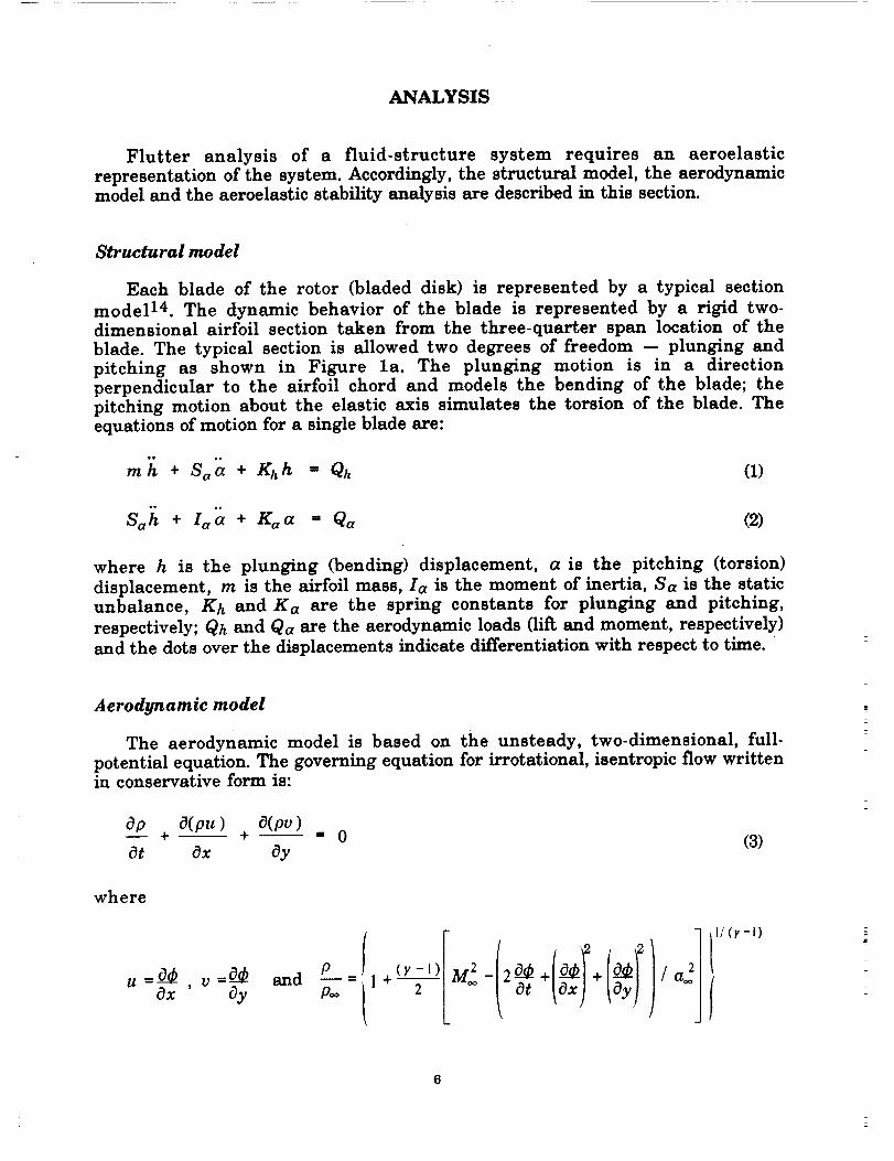
Each blade of the rotor (bladed disk) is represented by a typical section
model 14. The dynamic behavior of the blade is represented by a rigid two-dimensional airfoil section taken from the three-quarter span location of the
blade. The typical section is allowed two degrees of freedom -- plunging and
pitching as shown in Figure la. The plunging motion is in a direction
perpendicular to the airfoil chord and models the bending of the blade; the
pitching motion about the elastic axis simulates the torsion of the blade. The
equations of motion for a single blade are:
m'h + Saa + Khh -'- Qh (1)
+ + - (2)
where h is the plunging (bending) displacement, a is the pitching (torsion)
displacement, m is the airfoil mass, Ia is the moment of inertia, Sa is the staticunbalance, Kh and Ka are the spring constants for plunging and pitching,
respectively; Qh and Qa are the aerodynamic loads (lift and moment, respectively)
and the dots over the displacements indicate differentiation with respect to time.
Aerodynamic model
The aerodynamic model is based on the unsteady, two-dimensional, full-
potential equation. The governing equation for irrotational, isentropic flow writtenin conservative form is:
Op a(pu ) d(pv )+- + _ - 0 (3)
Ot Ox Oy
where
Ox, v =O_
dyand
poo t I ÷ IOXJ ay
l/
(r -I)
In these equations, ¢ is the velocity potential; p_, aoo and Moo are the density, sonic
velocity and Mach number, respectively, all evaluated at far upstream conditions.
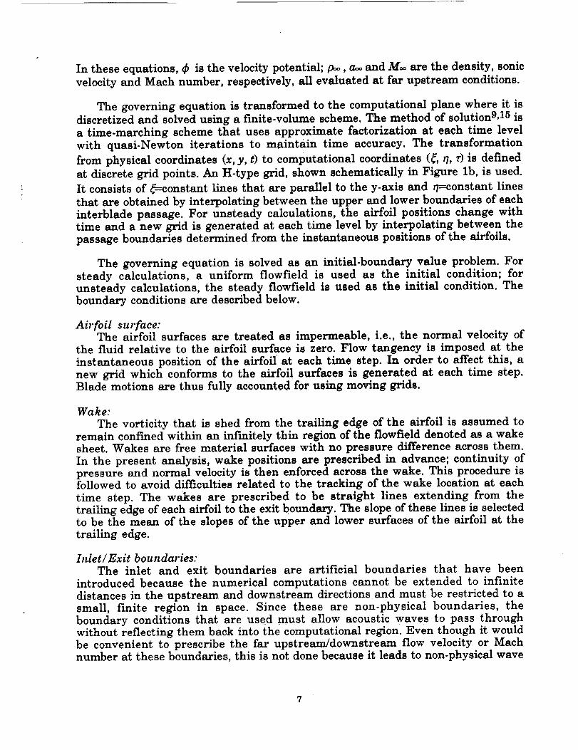
The governing equation is transformed to the computational plane where it is
discretized and solved using a finite-volume scheme. The method of solution 9,15 is
a time-marching scheme that uses approximate factorization at each time level
with quasi-Newton iterations to maintain time accuracy. The transformation
from physical coordinates (x, y, t) to computational coordinates (_, q, T) is defined
at discrete grid points. An H-type grid, shown schematically in Figure lb, is used.
It consists of _-constant lines that are parallel to the y-axis and r7---constant lines
that are obtained by interpolating between the upper and lower boundaries of each
interblade passage. For unsteady calculations, the airfoil positions change with
time and a new grid is generated at each time level by interpolating between the
passage boundaries determined from the instantaneous positions of the airfoils.
The governing equation is solved as an initial-boundary value problem. For
steady calculations, a uniform fiowfield is used as the initial condition; for
unsteady calculations, the steady flowfield is used as the initial condition. The
boundary conditions are described below.
Airfoil surface:The airfoil surfaces are treated as impermeable, i.e., the normal velocity of
the fluid relative to the airfoil surface is zero. Flow tangency is imposed at the
instantaneous position of the airfoilat each time step. In order to affect this, a
new grid which conforms to the airfoil surfaces is generated at each time step.Blade motions are thus fully accounted for using moving grids.
Wake:
The vorticity that is shed from the trailing edge of the airfoil is assumed toremain confined within an infinitely thin region of the flowfield denoted as a wake
sheet. Wakes are free material surfaces with no pressure difference across them.
In the present analysis, wake positions are prescribed in advance; continuity of
pressure and normal velocity is then enforced across the wake. This procedure isfollowed to avoid difficulties related to the tracking of the wake location at each
time step. The wakes are prescribed to be straight lines extending from the
trailing edge of each airfoil to the exit boundary. The slope of these lines is selectedto be the mean of the slopes of the upper and lower surfaces of the airfoil at the
trailing edge.
Inlet�Exit boundaries:
The inlet and exit boundaries are artificial boundaries that have been
introduced because the numerical computations cannot be extended to infinite
distances in the upstream and downstream directions and must be restricted to a
small, finite region in space. Since these are non-physical boundaries, the
boundary conditions that are used must allow acoustic waves to pass through
without reflecting them back into the computational region. Even though it would
be convenient to prescribe the far upstream/downstream flow velocity or Mathnumber at these boundaries, this is not done because it leads to non-physical wave
reflections. In the present analysis, characteristic boundary conditions 16 are used
at the inlet and exit boundaries. At the inlet/exit boundary, the Riemann
invariant corresponding to the incoming characteristic (positive characteristic
with respect to the inward normal) is prescribed based on the far
upstream/downstream conditions. This allows planar acoustic waves, which areat normal incidence to the boundary, to pass through without reflection. However,
the acoustic waves are generally not planar; also, they are generally not atnormal incidence to the boundary. _herefore, the use of one-dimensional
Riemann-invariant boundary conditions results in some wave reflections back
into the calculation domain.
Periodic boundaries:
Periodic conditions are imposed on grid lines extending from the leading edgeof the airfoil to the inlet boundary; see Figure lb. The periodic conditions are used
to simulate the fundamental periodicity present on the bladed disk in the
circumferential direction.
Additional details concerning the aerodynamic model and the boundaryconditions can be found in References 9 and 15.
Aeroelastic Stability
For a tuned cascade, in which all the blades are identical, the aeroelasticmodes consist of each of the N individual blades vibrating with equal amplitudes
with a f'Lxed interblade phase angle between adjacent blades 17. For the s th blade
vibrating in the r th interblade phase angle mode, this can be written as:
Ihs/b I
h o/bl i(wt*arS)ffi 6fO /
e S-0, 1,2 ..... N-i (4)
The phase angle between adjacent blades is given as
a r ffi 2rrr/N r - 0, 1, 2 ..... N-! (5)
The corresponding aerodynamic forces can be written as linear functions of the
displacements using the complex-valued frequency domain unsteady
aerodynamic coefficients lhh , lha, lab and la a :
where p = m/zp_b 2 is the mass ratio of the blade. The eigenvalue problem for the
tuned system can be written 18 as:
8
[[P]- [zl]{rl "{ol
where
[P]
g + lldtr l_ Xa + lhar-
(Wh/ )2
l_ X a + lah r
. .
(6)
In the above, Xa = Sa/mb is the distance between the elastic axis and center of
mass and ra-(Is�rob2) u2 is the radius of gyration about the elastic axis, both in
semi-chord units; Wh = (Kh /m) 1/2 and tOa = (Ks/Ia) 1/2 are the uncoupled natural
frequencies for bending and torsion, respectively; note, the subscript 's' which
identifies the blade has been dropped.
For each interblade phase angle mode, the solution of the above eigenvalue
problem results in two complex eigenvalues of the form
The real part of the eigenvalue (_) represents the damping ratio and the
imaginary part (v) represents the damped frequency; flutter occurs if p 2 0 for
any of the eigenvalues. The stability of each phase angle mode is examined
separately. The interblade phase angle is f'Lxed at one of the values given by
Equation (5) and the 2x2 eigenvalue problem is solved.
However, before the eigenvalue problem can be solved, the aerodynamic
coefficients must be calculated. For f'Lxed cascade geometric parameters, the
aerodynamic coefficients are functions of inlet Mach number (M_), reduced
frequency of blade vibration (kc) and interblade phase angle (ar). The following
procedure has been adopted for flutter calculations. A value of inlet Mach numberis selected. A value of reduced frequency is assumed and the aerodynamic
coefficients lhh, lha, lab and laa are calculated for all values of phase angle in
Equation (5). The eigenvalue problem is solved for each value of interblade phase
angle. The reduced frequency is varied until the real part of one of the eigenvalues
(_) becomes zero while the real part of the other eigenvalue is negative. The
assumed flutter reduced frequency (kcf) and the calculated flutter frequency (vf)
are both based on wf. Thus, these two can be combined to eliminate tcf and the
flutter reduced velocity (V'f) is obtained, viz., V*f = 2 -re/kcf. The critical phase
angle is identified as the one which results in the lowest flutter velocity. The
stability of a single-degree-of-freedom pitching system can be inferred entirely
9
from the imaginary part of the moment coefficient, Im{laa}; flutter occurs if
Im{la a } _ O.
Aerodynamic Coefficients
The calculation of the frequency domain unsteady aerodynamic coefficients
(lhh, lha, lab and la a ) is described next. For a given cascade geometry and inlet
Mach number, these coefficients are required for plunging and pitching motions
of specified frequency and specified interblade phase angle (restricted by Equation(5)). The full-potential solver is based on a time-marching algorithm and threedifferent methods of calculating the aerodynamic coefficients are described.
1. Harmonic Oscillation Method
In the Harmonic Oscillation (HO) method 12, all the N airfoils are oscillated
with the specified frequency and specified interblade phase angle. The motion of
the s th airfoil in the cascade is prescribed to be of the form:
or
h - h o sin(w t+Sar) " ho sin(kcM.or +sa_)
a = % sin(w t+sar) = % sin(kcM_r+sar)
for plunging
for pitching
Calculations are started from a steady flowfield and continued until starting, non-
periodic, transients have decayed and the fiowfield has become periodic in time.The lif_ and moment acting on the reference airfoil (s--0) are calculated at every
time step and later decomposed into Fourier components. If the amplitude ofoscillations is sufficiently small, it can be shown by a perturbation analysis that
the flowfield will have the same harmonic time dependence as the motion 7.
Therefore, the lift and moment coefficients (Cl and Cm) on the zeroth blade can be
represented in terms of a complex quantity Q0as [Im{Q0}cos(wt)+
Re{Q0} sin(w t) ]. The frequency dom_n-unsteady aerodynamic c0efficients (lhh,
lha, lab and laa ) are then obtained by dividing Q0 by kc 2, the amplitude of motion
and other constants. The harmonic oscillation method requires that calculations
for each of the N values of interblade phase angle be done separately. It is possible
to reduce this computational effort by using the Influence Coefficient method
described next,
2. Influence Coefficient Method
The Influence Coefficient (IC) method is based on the principle of linear
superposition. Briefly, the solution to a problem is obtained by superposing thesolutions to the individual elemental problems that comprise the original
problem. Since the method is based on the principle of linear superposition, it is
valid only for linear problems. It can be shown that the unsteady part of the
present problem is linear (governed by a linear differential equation) for
10
sufficiently small amplitude of oscillation. 7 It should be emphasized that only the
unsteady part of the problem is linear; the steady flowfield is described by a
nonlinear equation.
Since the quantities of significance are the lii'_ and moment coefficients, the
following discussion will deai only with a general integrated force quantity.
However, the results obtained can be extended by analogy to pressure distributionsor the distribution of other flow variables. Also, complex notation is used for
convenience; in this notation it is implied that only the imaginary part of the
complex quantity is to be considered. For example, when the motion is specified to
be of the form hoe i°° t, it is understood that the motion is actually hosin(w t).
The problem to be solved consists of a cascade of N blades in which each blade
oscillates with a motion of the form sin(w t+Sar), where s is the blade index that
varies from 0 to N-1, and ar is the interblade phase angle given by Equation (5).
This problem is divided into N elemental problems. The k th elemental problemconsists of the same cascade of N blades in which the k th blade oscillates with a
motion of the form sin(w t) while all other blades remain stationary. The original
problem and all the elemental problems have solutions that are harmonicfunctions of time.
For the problem in which all blades oscillate with a motion of the form
ei(Wt+sar),the forces (cland cm) on the 0th blade can be represented as Qo eiw t;Qo
is complex valued to allow the force to lead or lag the motion. The forces on the 0th
blade in the k th elemental problem can be represented as Qo, k eiwt; Q0,k is
sometimes referred to as an influence coefficient. Thus, using superposition, the
following relation can be obtained.
N-I
QoeiWt = Z Qo, k eiWt eikar (8)k-0
Now, due to the periodicity of the cascade, only the relative positions of the
oscillating blade and the reference (zeroth) blade are important. That is, the forces
generated on the 0 th blade due to the oscillation of the k th blade are equal to the
forces on the Ist blade due to the oscillation of the k+l th blade, and so on. Thus,
Qo, k ffi Q-k,O ffi QN-k,O (9)
where the periodicity of the cascade of N blades has been invoked again in the last
step. Thus, the solution to the problem in terms of the influence coefficients can be
written as:
N
Qo eiwt= _ QN-k,o eiWte ikar (10)k=l
11
Replacing the influence coefficients Qo, k by the coefficients QN-k,O means that
all the required influence coefficients can be determined simultaneously rather
than separately. Thus, instead of oscillating the k th blade, calculating the
pressure history on the zeroth blade and then repeating for all values of k between0 and N-1, it is possible to oscillate the zeroth blade and calculate the pressures on
all the blades simultaneously. This means that the computational effort required
for the calculation of all the influence c qefficients can be reduced by a factor of Nover the Harmonic Oscillation method. '
It should be noted that the elemental problem used in the present work is
different from the one used more frequently, in which a single blade in an infinite
cascade is oscillatedl9, 20. In the present work, periodic boundary conditions are
used to simulate an infinite cascade using N blades in the calculations. Thus,
when a single blade in the N-blade cascade is oscillated, it corresponds to every
N th blade in the infinite cascade being oscillated. The expressions presented in
this section are exact for the discrete values of interblade phase angle given by
Equation (5) and approximate for all other values. Although the summation in
Equation (8) only extends over a finite number of terms, it does not represent atruncation of an infinite sum as long as the value of interblade phase angle is
restricted by Equation (5). Calculations performed without using periodic
boundary conditions simulate a finite section of an infinite cascade surrounding
the blade that is being oscillated. This introduces an approximation into such
calculations for all values of interblade phase angle; however, this error
decreases rapidly as the number of blades used in the calculations is increased.
3. Pulse Response Method
For a given motion, plunging or pitching, the Harmonic Oscillation method
and the Influence Coefficient method require separate calculations for each
oscillation frequency of interest. In order to reduce the computational effort, the
Pulse Response (PR) method described in this section can be used; this method
has evolved from the indicia1 approach that is widely used in many differentfields.
Researchers have investigated the indicial approach for aerodynamic
calculations with isolated airfoils21 and cascades 22. The indicial response is the
response, liftor moment, to a step change in the given mode of motion. From the
indicial response, the response for any arbitrary motion, specifically harmonic
motion, can be calculated using Duhamel's superposition integral. Let the time-
dependence of the blade motion (plunging or pitching) be denoted as f(t) and let
the corresponding response (liftor moment) be denoted as F(t). Let Fo (t) denote
the response corresponding to a unit step function, f(t)= 5(t). The response
corresponding to an arbitrary motion f(t) can then be written using Duhamers
superposition integral as
_0 tF(t) = F5(t-_) _) d_ (Ii)
12
Using the above equation, the response to a harmonic motion, f(t)= e iw t, can bedetermined. Since only the periodic.response is of interest, the limit of the above
integral as t--*_ is considered. Using a change of variable and extending the
lower limit to -_, the following relation can be obtained
t) = iw (w)eiwt (12)
where F-_o(w) is the Fourier transform of F5 (t) given by
= f+_ F_(t) e- iwt dt (13)
The indicial response method has the following drawback. The step change in
the displacement results in infinite velocity at the time at which the step changeoccurs. The indicial response contains a large spike at this time. Therefore, very
small time steps must be used to ensure that the results are accurate during this
period of rapid transients and the accurate evaluation of the Fourier integral overthis time interval is difficult. In addition, the treatment of this infinite velocity by
finite differences leads to non-physical transients that can cause errors in the
final results. To avoid these difficulties, researchers 23 have replaced the step
function by a smooth version which does not result in infinite velocities and
spikes. Polynomial functions of time have been used in place of the standard stepfunction to obtain the necessary smoothness at the beginning and end of the step.
This allows time steps of normal size to be used in the calculations.
For an arbitrary motion f(t) and the corresponding response F(t), the Fourier
transform of Equation (11) gives24:
= / (14)
where f(w) and F(w) are the Fourier transforms of f(t) and F(t), respectively. It
should be noted from Equation (12)that iwF_(w) gives the response to a harmonic
motion. Since only the response to a harmonic motion is to be obtained, any
arbitrary motion and the corresponding response can be used to obtain iwF_(w)
from Equation (14).
Thus, the time variation of both the motion and the response are required to
calculate the response to harmonic motions. To reduce the time required for the
transients to decay, the smooth step is often replaced by a pulse 25. In the pulse
motion, the blade returns to its original position after the duration of the pulse.
This is in contrast to the step motion in which the blade position is different before
and after the step. The pulse motion thus allows the flowfield to return to its
steady undisturbed state after the transients created by the pulse have decayed.
The unsteady calculations therefore need to be carried out only long enough to
13
ensure that the solution has reached its fmal state (the same as the initial state)
within some specified tolerance.
Several smooth pulse shapes have been investigated by researchers. A
comparison 3 of results from three different pulse shapes shows that although the
shape and size of the pulse determines the transient response, the ratio of the
Fourier transforms of the response an.d the motion remains unchanged. Thus,
the shape of the pulse is not of particular importance although care must be taken
to ensure that the transform of the pulse motion does not become zero in the
frequency range of interest. In addition, the duration of the pulse must be selected
according to the range of frequencies of interest. Thus, the harmonic time periodof interest must be smaller than the duration of the pulse for the results to be
meaningful. This places a lower limit on the values of frequency for which
calculations can be made using a pulse of given duration. The upper limit on the
frequency is determined by the size of the time step; the upper limit is generally
not relevant because the time step is normally quite small for reasons of
numerical stability and accuracy.
In the present calculations, the pulse function is selected as:
()21)4 _L__ exp 2 1 forO < t< tmaxfit) = t,,,_ 1 - t It,,,=,
f(t) = 0 for t > tmax (15)
where tmax is the duration of the pulse. The above choice makes f(t) and t'(t)
vanish at t=O and t=tmax; in addition, higher derivatives also go to zero att=tmax. This ensures that there is a smooth transition to and from theundisturbed blade position.
The Pulse Response method is used in conjunction with the Influence
Coefficient method as follows. One blade in the cascade is given a transient
motion of the form h(t)- ho f(t) or a(t)- ao f(t). The calculations start with the
steady solution and unsteady response to the pulse in either motion, plunging or
pitching, is calculated until the transient flowfield reaches the steady flowfield
within a specified tolerance. The motion as well as the responses on all the bladesare recorded and Fourier transforms of these are calculated numerically for the
frequency of interest. Using these transforms, the influence coefficients (Qk,0) are
calculated from Equations (14); it is to be noted that the harmonic response,
iwF-_(w), obtained from Equation (14) for this case, is simply the influence
coefficient, Qk,0. Equation (10) is then used to calculate the frequency domain
unsteady aerodynamic coefficients (lhh, lha, lah and laa ) for the interblade
phase angle of interest. In this way, the coefficients can be determined for variousvalues of reduced frequency by recalculating the Fourier transforms for the
frequency of interest using the same time histories.
14
RESULTS AND DISCUSSION
The results are presented in two parts. The results in the initial part serve tovalidate the Influence Coefficient method and the Pulse Response method by
comparison with the Harmonic Oscillation method. In the remaining part of this
section, results of flutter calculations for two examples are presented.
Calculation of Aerodynamic Coefficients
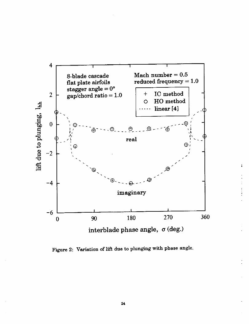
Figure 2 shows the unsteady lift coefficient due to plunging motion in a
cascade comprised of eight flat plates. The cascade is unstaggered and has a
unity gap-to-chord ratio. The Mach number of the flow at the inlet is Moo-0.5 and
the reduced frequency of oscillation is ke=l.0. A 41x21 grid is used in the
calculations with 41 points in the streamwise direction and 21 points in the
direction of the stagger line in each of the 8 interblade passages; 21 points are
located on each (upper and lower) surface of each airfoil; all grid points are
uniformly distributed. 150 time steps/cycle of oscillation are used which
corresponds to a nondimensional time step of 0.084 and the calculations arecontinued for three cycles of blade oscillation to allow non-periodic starting
transients to decay. The amplitude of oscillation used is ho/c-0.002 which is
found to be small enough to yield a response which is linearly dependent on the
amplitude of motion.
The results obtained from the IC method and the HO method are represented
as open symbols; the results from classical linear theory 4 are shown as dashedlines and denoted as 'linear [4]'. A comparison of the various results reveals the
following. The HO method and the IC method yield virtually identical results.
This is simply a verification of the superposition principle and the associated
calculations. It implicitly confirms that the unsteady problem is linear for the
amplitude of motion used in the calculations. Similar comparisons made withother airfoils and other cascade geometries have demonstrated the same level of
agreement seen here. The results of the present calculations also agree quite wellwith the results from classical linear theory. For fiat plate airfoils and small
amplitude oscillations, the present calculations are expected to yield the sameresults as obtained from classical linear theory. It is to be noted that classical
linear theory uses a semi-analytical formulation and the solutions show singular
behavior near the leading edge. This feature is not completely captured by the
relatively coarse 41 x21 grid used in the present calculations. This may account for
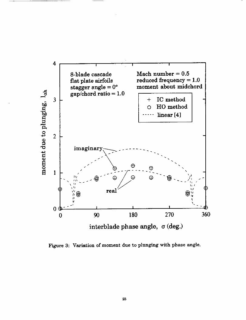
some of the differences observed between the results. Figure 3 shows the moment
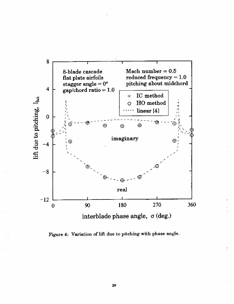
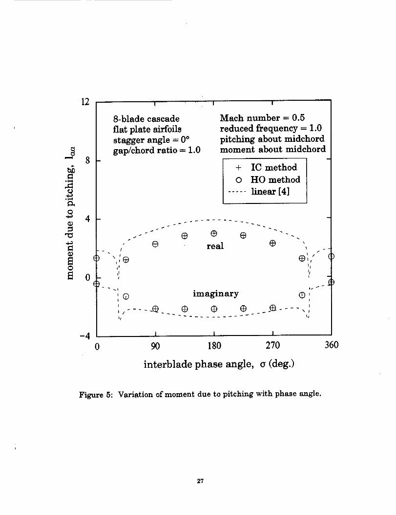
coefficient for the plunging motion. Figures 4 and 5 show the lift and moment
coefficients due to pitching about midchord; the amplitude of pitching oscillations
used in the calculations is ao = 0.2 ° and 210 time steps/cycle of oscillation are used.
In all the above results, the agreement between the HO method and the IC method
is extremely good. The agreement between the present results and those from
classical linear theory ranges from fair to good.
15
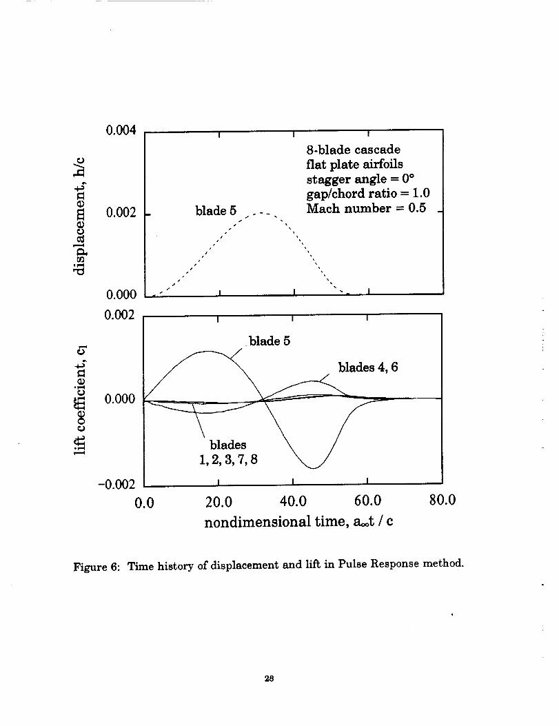
Figure 6 shows the time-variation of the displacement and the resulting lift onall the blades of a 8-blade cascade of fiat plates for use in the PR method. The grid
and the time step used are the same as those used in the previous calculationswith the HO method and the IC method. The motion of blade 5 is shown as a
function of time; the other blades in the cascade remain stationary. The
maximum displacement during the pulse is ho/c = 0.002 and the duration of the
pulse is t,_ax = 20_. The lift on all blades is shown separately. As can be seen, the
calculations are continued until all responses have returned to the initial
undisturbed values. For the present calculation, the initial and final response
levels correspond to zero lift since the airfoils are fiat plates. If the calculations
are for a configuration which has a non-zero value of steady state lift, thensimilar variations wili be obtained for the unsteady component of the lift
(instantaneous lift minus steady lift). The time histories are Fourier transformed
and combined according to Equati0n (14) to obtain the influence coefficients
(QN-k,0) which are combined according to Equation (10) to get the harmonic
coefficients.
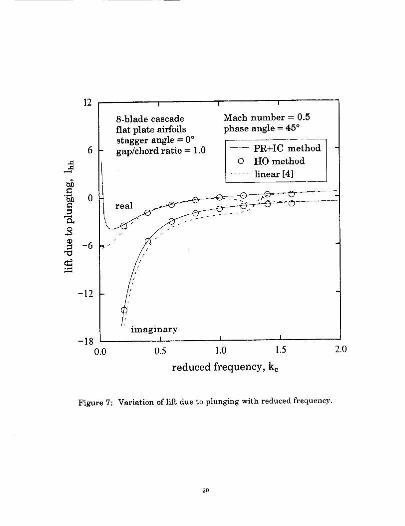
Figure 7 shows the lift due to plunging obtained by applying the PR methodand the IC method to the time histories of Figure 6. The solid lines are results
from the PR+IC method and the open symbols represent results from the HOmethod. Results from classical linear theory are also shown for comparison. The
agreement between the PR+IC method and the HO method is very good. Thissubstantiates the validity of the PR method used in combination with the IC
method. It also implicitly confirms the linearity of the unsteady problem which
permits the use of the Duhamel superposition integral and the influencecoefficient approach. The agreement between the present calculations and theresults from classical linear theory is also quite good except at values of reduced
frequency near the point of acoustic resonance. The comments made earlier
regarding the singularity near the leading edge and the limitations of the grid
used in the present study can be applied to account for some of the observed
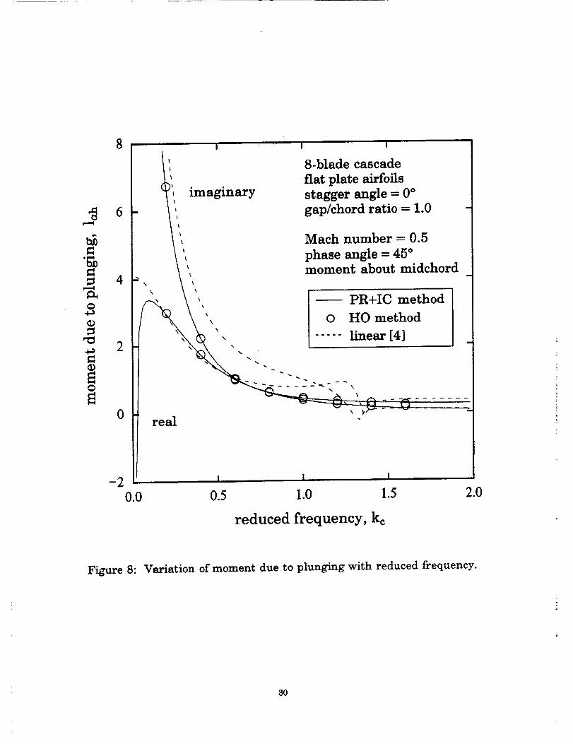
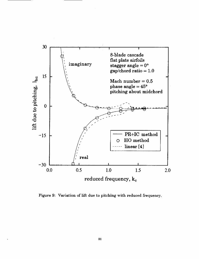
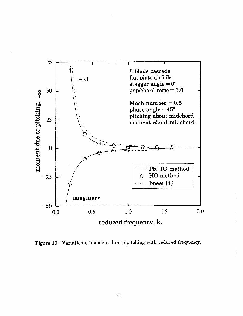
discrepancy. Figures 8-10 show the variation of the remaining coefficients for thesame cascade and flow condition. As before, the agreement between the PR+IC
method and the HO method is very good and the agreement between the presentresults and those from classical linear theory varies from fair to good.
All the computations described here were performed on a CRAY X-MP
computer. The calculations performed using the HO method required about 160
CPU seconds for the case of pitching motion with kc-l.0 and _=45 °.
Approximately the same amount of time was required for the corresponding
calculations using the IC method with kc=l.0 which gave results for
o'_-0°, 45 °, 90 °,...,315 °. The calculation of the time histories in the PR method
required about 230 CPU seconds; the additional time required for calculating
Fourier transforms was quite small and was not recorded.
16
Calculation of Flutter Boundaries
Flutter results are presented for two examples. The first example is a single-
degree-of-freedom (pitching) system that has been previously considered in
References 2 and 12. The cascade has nine blades, a stagger angle of {_-45 °, a gap-
to-chord ratio of g/c-l.O and the elastic axis is located at the leading edge
(ah=-1.0). The stability of this system can be inferred entirely from the imaginary
part of the moment coefficient, Im{/a a }.Flutter occurs if Im{la a }_ 0 in which
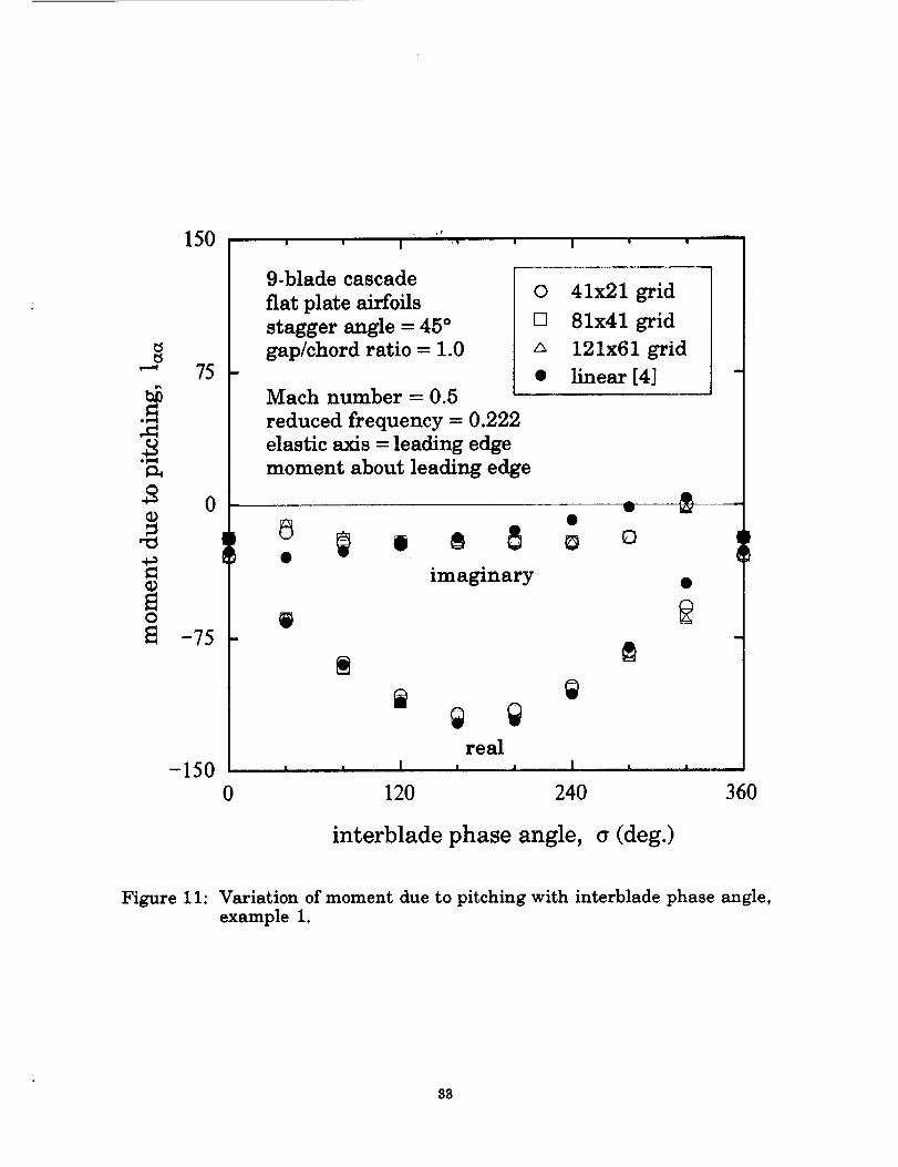
case the oscillating cascade extracts energy from the fluid stream. Figure 11
shows the moment coefficient (real and imaginary parts) at the different values of
interblade phase angle that may arise at flutter (Equation (5)).The results are for
an inlet Mach number of Mo_=0.5 and a reduced frequency of kc=0.222.
Calculations have been performed on three different grids with 41 x21, 81 x41, and
121 x61 points in each interblade passage; the number of grid points on each airfoil
surface (upper and lower) is 21, 41 and 61, respectively. The results from classical
linear theory are included for comparison.
It can be seen from Figure 11 that a uniform refinement of the grid spacing by
a factor of 3 results only in small changes in the value of the moment coefficient.
Some discrepancy is also observed between the present results and the results
obtained from classical linear theory; this difference is not always reduced by grid
refinement. This indicates that some other cause exists for the observed
discrepancy. Efforts are currently underway to resolve this difficulty; no
explanation is offered at present. It should be noted that observed differencecannot be attributed to the use of the PR method or the IC method since these have
been validated by comparison with the HO method.
For the calculations performed using the 41 x21 grid, a reduced frequency of
kc=0.222 results in neutral stability CIm{laa } = 0) of the offi320 ° aeroelastic mode
with all other modes being stable (Im{laa } < 0); this result was obtained after
calculating the coefficient laa at different values of reduced frequency and
interblade phase angle. Thus, the reduced frequency at flutter is kcf-=0.222 and the
phase angle at flutter is crf=320 °. The corresponding results from classical linear
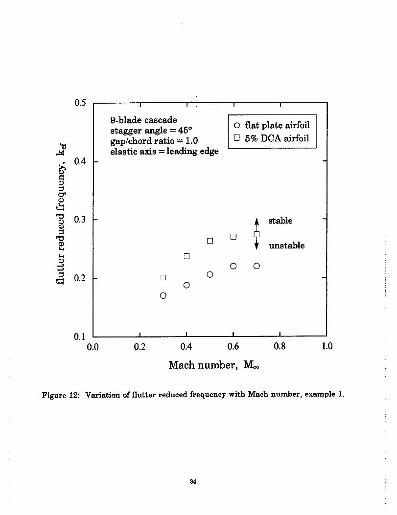
theory are kef=0.254 and _f=320 °. Similar calculations have been performed for
other values of the inlet Mach number between 0.2 and 0.8 using a 81 x41 grid in
each interblade passage. Figure 12 shows the variation of flutter reduced
frequency with Mach number. It can be seen that the reduced frequency at flutter
increases with the inlet Mach number with a levelling-off at the higher values of
Mach number. In addition to the flat plate airfoil, results are also shown for adouble-circular-arc airfoil with thickness-to-chord ratio of 0.05 (5% DCA airfoil).
These calculations have also been performed with a 81 x41 grid in each interblade
passage. In the present example, the effect of thickness is to increase the flutter
reduced frequency at all the values of inlet Mach number. The interblade phase
angle at flutter was found to be _rf=320 ° for all the results shown.
17
The second example for which flutter calculations have been performed
consists of a 5-blade cascade in which the typical section has two degrees-of-
freedom. This example has been previously considered in Reference 2; the
geometric and structural parameters in this example are representative of the
SR5 propfan 13. The cascade stagger angle is 0=10.7 ° and the gap-to-chord ratio is
g/c=1.85. The airfoil section is from a NACA 16 series with a thickness-to-chord
ratio of 0.03 and a design lift coefficient .of 0.3; this airfoil, which is taken from the
three-quarter span location of the SR5 propfan, is hereai_er referred to as the SR5
airfoil. The structural model for each blade is a two-degrees-of-freedom typical
section with elastic axis at the leading edge (ah--l.O). The mass ratio is/_=115, the
radius of gyration is ra _1.076, the offset between elastic axis and center of mass is
Xa _0.964 and the ratio of uncoupled natural frequencies in bending and torsion is
wh/wa _0.567.
The following procedure has been used in the calculations. For each value of
interblade phase angle obtained from Equation (5), the reduced frequency is varied
until one of the two eigenvalues of Equation (7) displays neutral stability (g=0)
while the other eigenvalue displays stability (_0). The reduced frequency thus
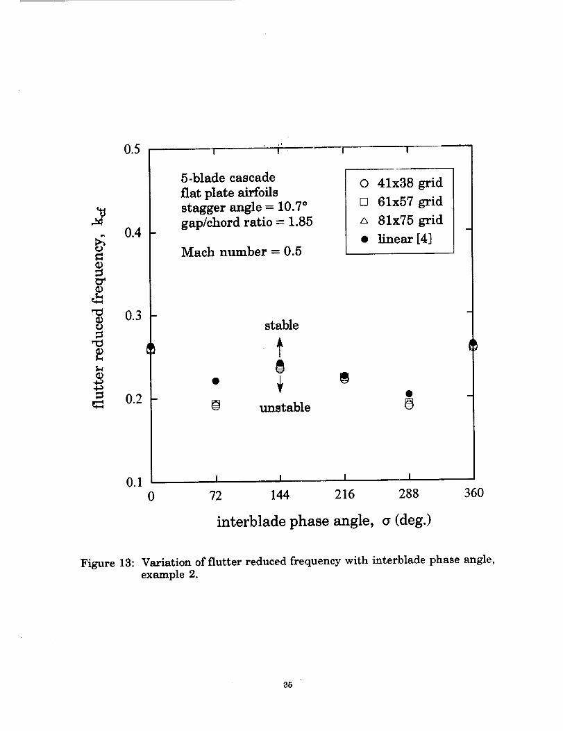
obtained (kcf) is shown in Figure 13 for a fiat plate airfoil. Calculations have been
done using three different grids with 41 x38, 61 x57, and 81 x75 points in each ofthe
five interblade passages; the number of grid points on each airfoil surface (upper
and lower) is 21, 31 and 41, respecti,eely. Results from classical linear theory are
included for comparison. It can be seen that reducing the grid spacing by a factor
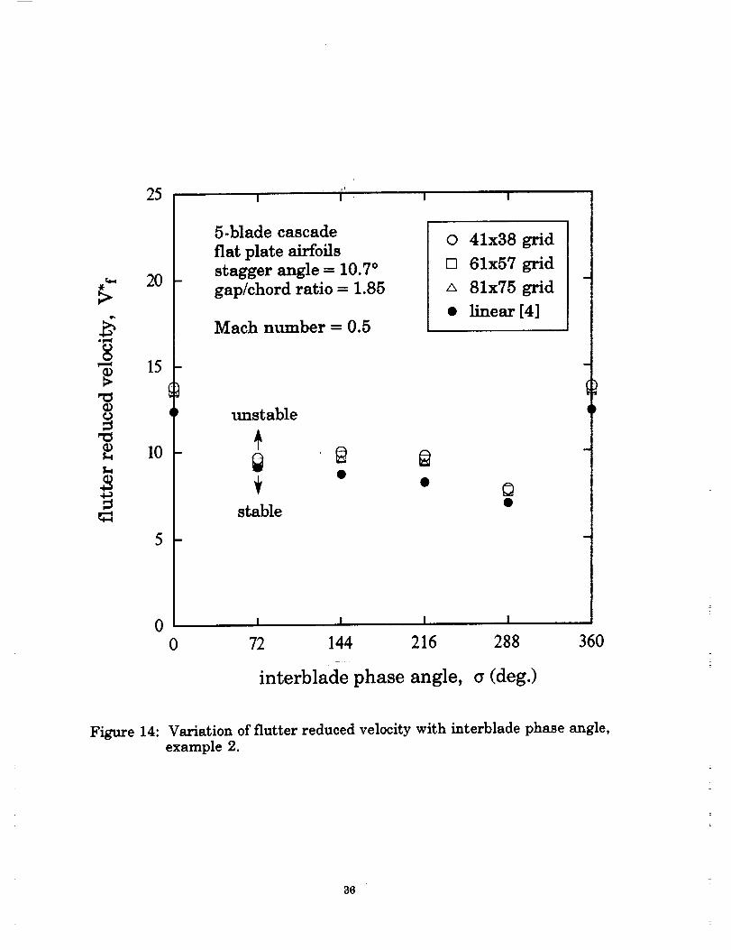
of 2 does not result in much change in the reduced frequency at flutter. Figure 14
shows the flutter reduced velocity for the same case. It can be seen that the lowest
flutter reduced velocity occurs at o=288 ° and this is identified as the critical phase
angle. The corresponding flutter reduced velocity is V*f- 7.82 for the 41x38 grid,
V*f ffi 7.71 for the 61 x57 grid and V*f ffi 7.63 for the 81 _75 grid; the result from
classical linear theory is V*f- 7.01.
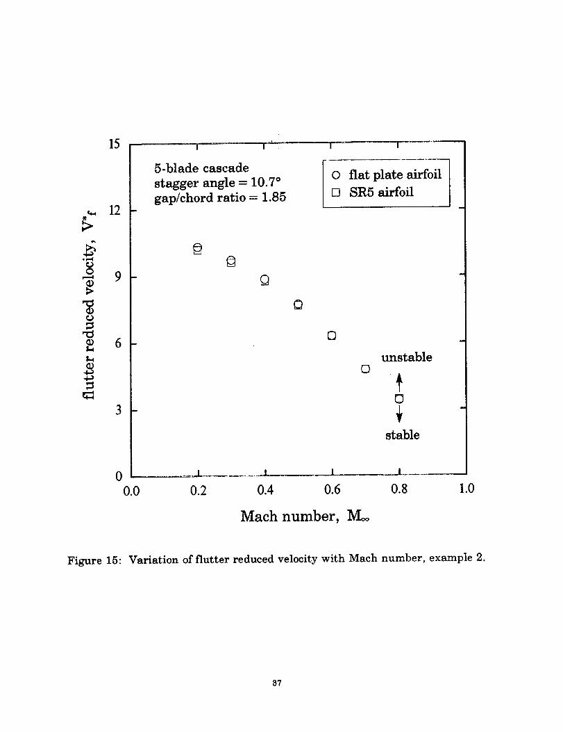
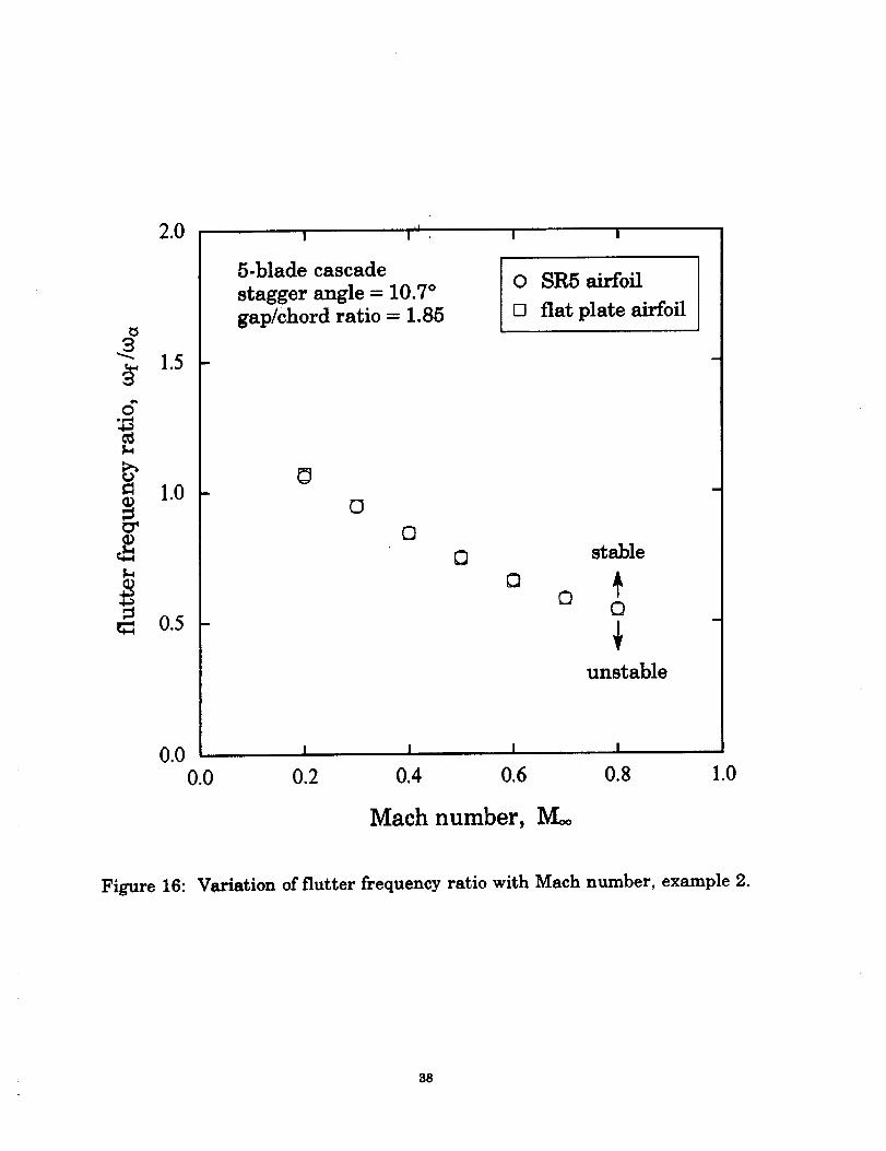
Similar calculations have been performed for values of inlet Mach number
between 0.2 and 0.8; a 61_57 grid is used. Calculations are done for a flat plate
airfoil and the SR5 airfoil.The results are presented in Figures 15 and 16 as
variations of flutter reduced velocity (V'f) and flutter frequency ratio (wf/wa) with
Mach number. Figure 15 shows that the flutter reduced velocity decreases with
increasing Mach number for both the flat plate airfoil and the SR5 airfoil;the
variation is seen to be almost linear. Figure 16 shows that the flutter frequency
ratio also decreases with increasing Mach number. It is noted that there is only a
marginal difference between the results for the flat plate and the SR5 airfoil.
However, itmay be recalled that the SR5 airfoilhas a small camber angle, a small
thickness-to-chord ratio of 0.03 and the cascade gap-to-chord ratio is large
(g/c=1.85). Therefore, it may be concluded that there is not much steady flow
deflection for this case and consequently the flutter results do not show much
difference between the flatplate airfoiland the SR5 airfoil.
18
CONCLUDING REMARKS
Two methods of calculating (linear) frequency domain unsteady aerodynamic
coefficients from a time-marching full-potential solver have been developed and
verified. The first method, the Influence Coefficient method, allows coefficients
for different interblade phase angles to be calculated simultaneously. The second
method, the Pulse Response method, _llows coefficients for several oscillation
frequencies to be calculated from the same transient response. When these twomethods are combined, the aerodynamic coefficients for several combinations of
phase angles and frequencies can be calculated at approximately the
computational cost required for the calculation of a single phase angle and singlefrequency using the Harmonic Oscillation method. These methods have beenverified individually and in combination by comparison with the Harmonic
Oscillation method. For small amplitudes of motion, the unsteady flow problem is
linear and therefore these methods give accurate results, as expected.
Flutter calculations have been performed for two examples. The first example
has only pitching degree of freedom. Calculations have been done over a range of
subsonic Mach numbers using a flat plate airfoil and a 5% thick double-circular-arc airfoil. For both airfoils, the flutter reduced frequency is seen to increase with
Mach number and the effect of airfoil thickness is to increase the flutter reduced
frequency. The results obtained from the present calculations with a fiat plate
airfoil show some differences when compared with the results from the classical
linear theory. These differences are not eliminated by grid refinement indicatingthat some other cause contributes to this discrepancy. However, there is no
indication that the problem lies in the use of either the Influence Coefficient
method or Pulse Response method.
The second example for which flutter calculations have been performed is a
two-degree-of-freedom system with geometric and structural parameters
representative of the SR5 propfan. Once again, calculations have been performed
over a subsonic range of Mach numbers. The flutter reduced velocity and the
flutter frequency ratio are seen to decrease continuously with increasing Machnumber; the decrease in flutter reduced velocity is almost linear with Machnumber. The difference between the results for the flat plate and the SR5 airfoil
are negligible. It is inferred that the combination of large gap-to-chord ratio,small thickness-to-chord ratio and small camber angle results in very little mean
flow deflection and consequently there is very little change in the unsteady
aerodynamic behavior due to the addition of loading.
The present approach allows a unified analysis capability in which both time
domain and frequency domain flutter calculations can be performed using the
same time-marching algorithm. This will allow a direct comparison of resultsfrom linear and nonlinear flutter analyses without concern for differences in CFD
algorithms, grids and other purely numerical factors. The computationalefficiency that is provided by these methods will allow flutter calculations to be
done more routinely than was previously possible with the Harmonic Oscillation
method. The methods implemented here on a full-potential solver can just as
19

easily be applied to other time-marching analyses, such as those based on the
Euler equations. Although the present work has been restricted to subsonic Machnumbers, transonic flow calculations can also be performed using the same
methods.
2O
REFERENCI_
1 Mehmed, O., Kaza, K. R. V., Lubomski, J. F., and Kielb, R. E., "Bending-Torsion Flutter of a Highly Swept Advanced Turboprop," NASA TM 82975, 1982.
2 Bakhle, M. A., Reddy, T. S. R., .Keith, T. G., Jr., "Time Domain FlutterAnalysis of Cascades Using a Full-Potential Solver," AIAA Paper 90-0984, Apr.1990. To be published in AL4A Journal, July 1991.
3 Williams, M. H. and Ku, C. C., "Three Dimensional Full PotentialAerodynamic Method for the Aeroelastic Modeling of Propfans," AIAA Paper 90-1120, Apr. 1990.
4 Smith, S. N., "Discrete Frequency Sound Generation in Axial FlowTurbomachines," British Aeronautical Research Council, London, ARC R&MNo. 3709, 1971.
5 Lane, F, "Supersonic Flow Past an Oscillating Cascade with SupersonicLeading-Edge Locus," Journal of the Aeronautical Sciences, Vol. 24, Jan. 1957,pp. 65-66.
6 Whitehead, D. S. and Grant, R. J., "Force and Moment Coefficients for HighDeflection Cascades," Proc. 2nd Intl. Symp. on Aeroelasticity in Turbomachines,(ed. P. Suter), Juris-Verlag Zurich, 1981, pp. 85-127.
7 Verdon, J. M. and Caspar, J. R., "Development of a Linear AerodynamicAnalysis for Finite-Deflection Subsonic Cascades," A/AA Journal, Vol. 20, No. 9,Sep. 1982, pp. 1259-1267.
8 Hall, K. C. and Crawley, E. F., "Calculation of Unsteady Flows inTurbomachinery Using the Linearized Euler Equations," A/AA Journal, Vol. 27,
No. 6,June 1989, pp. 777-787.
9 Kao, Y. F., "A Two-Dimensional Unsteady Analysis for Transonic and
Supersonic Cascade Flows," Ph.D. Thesis, School of Aeronautics andAstronautics, Purdue University, West Lafayette,Indiana, May 1989.
IO Huff, D. L., "Numerical Analysis of Flow Through Oscillating Cascade
Sections,"AIAA Paper 89-0437, Jan. 1989.
11 Reddy, T. S. R., Bakhle, M. A., and Huff, D. L., "Flutter Analysis of a
Supersonic Cascade in Time Domain Using an Euler Solver," NASA TM in
preparation, 1990.
12 Bakhle, M. A., Keith, T. G. Jr., and Kaza, K. R. V., "Application of a Full-Potential Solver to Bending-Torsion Flutter in Cascades," AIAA Paper 89-1386,
Apr. 1989.
21
13 Reddy, T. S. R., Srivastava, R., and Kaza, K. R. V., "The Effects of RotationalFlow, Viscosity, Thickness, and Shape on Transonic Flutter Dip Phenomena,"
AIAA Paper 88-2348, Apr. 1988.
14 Bisplinghoff,R. L. and Ashley, H., "Principles of Aeroelasticity,"John Wileyand Sons, Inc.,New York, 1962.
16 Shankar, V., Ide, H., Gorski, J., and Osher, S., "A Fast Time-AccurateUnsteady Full Potential Scheme," AIAA Paper 85-1512, Aug. 1985.
16 Hedstrom, G. W., "Nonreflecting Boundary Conditions for Nonlinear
Hyperbolic Systems," Journal of Computational Phys/cs,Vol. 30, 1979, pp. 222-237.
17 Lane, F., "System Mode Shapes in the Flutter of Compressor Blade Rows,"Journal of the Aeronautical Sciences,Vol. 23, Jan. 1956, pp. 54-66.
18 Bendiksen, O., and Friedmann, P., "Coupled Bending-Torsion Flutter inCascades," A/AA Journal, Vol. 18, No. 2, Feb. 1980, pp. 194-201.
19 Nixon, D., Tzuoo, K. L., and Ayoub, A., '_Rapid Computation of UnsteadyTransonic Cascade Flows," AYAA Journal, Vol. 25, No. 5, May 1987, pp. 760-762.
20 Buffum, D. H., and Fleeter, S., "Aerodynamics of a Linear OscillatingCascade," NASA TM 103250, Aug. 1990.
21 Ballhaus, W. F. and Goorjian, P. M., "Computation of Unsteady TransonicFlows by the Indicia1Method," A/AA Journal, Vol. 16, No. 2, Feb. 1978, pp. 117.124.
22 Kerlick, G. D. and Nixon, D., "A High-Frequency Transonic SmallDisturbance Code for Unsteady Flows in a Cascade," AIAA Paper 82-0955, June1982.
23 Myers, M. R. and Ruo, S. Y., "Calculation of Unsteady AerodynamicCoefficientsUsing Transonic Time Domain Methods," AIAA Paper 83-0885, Apr.1983.
24 Davies, D. E. and Salmond, D. J., "Indicial Approach to HarmonicPerturbations in Transonic Flow," A/AA Journal, Vol. 18, No. 8, Aug. 1980, pp.1012-1014.
25 Seidel,D. A., Bennett, R. M., and Whitlow, W., Jr.,"An Exploratory Study ofFinite-DifferenceGrids for Transonic Unsteady Aerodynamics," AIAA Paper 83-
0503, Jan. 1983.
22
b I bj
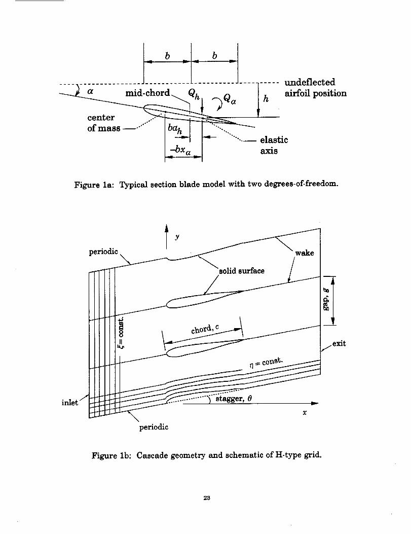
center____ _ofmass--"" __
--_ "'""",.--elastic
"b x a a_s
undeflected
airfoil position
Figure la: Typical sectionblade model with two degrees-of-freedom.
Figure Ib: Cascade geometry and schematic of H-type grid.
23
4
2
"6 0
Ch
O
-4
-6
C
m
ii i
I
8-blade cascade
fiatplateairfoils
stagger angle = 0°
gap/chord ratio= 1.0
\
I
A /
,@I
Mach number = 0.5
reduced frequency = 1.0
+ IC methodO HO method
..... linear [4]
_-- -. • .... p_.... __--- -_"
real
I
j
"®- O
imaginary
/
/
1
@,t
/
f
f
/
/
I I I
0 90 180 270
interblade phase angle, a (deg.)
C_
360
Figure 2: Variation of lif_due to plunging with phase angle.
24
4
2
0
i
8-blade cascade
flat plate airfoils
stagger angle = 0 °
gap/chord ratio = 1.0
Mach number = 0.5
reduced frequency = 1.0moment about midchord
+ IC method
O HO method
..... linear [4]
@@
;--.$ ,,,\ II _I I
'I IJ III
,;:$ rea _ ,,,Itif qII! _I
l- I I I
0 90 180 270
m
/
/
)
)
360
interblade phase angle, a (deg.)
Figure 3: Variation of moment due to plunging with phase angle.
25
8
4
•_ 0
,1=-I
C)
_ -4
-8
-12
m
E(
0
'* 'l
8-blade cascade
fiat plate airfoilsstagger angle = 0 °
gap/chord ratio = 1.0
11
11
I t
/
II I
@
\
%
®.
Mach number = 0.5
reduced frequency = 1.0pitching about midchord
+ IC method
O HO method
..... linear [4]
@ @ @
imaginary
r
II
II
II
II
I I
I _ \
I
I
(9,
t
I
s.J
/
/
f
.@J
JJ
real
! ! I
90 180 270 360
interblade phase angle, a (deg.)
Figure 4: Variation of lift due to pitching with phase angle.
26
O
12
8
4
0
8-blade cascade
fiat plate airfoils
stagger angle = 0 °
gap/chord ratio = 1.0
m
js
..-" @ @
-. " _9 real",:e
i I
$1
1
E
I
Mach number = 0.5
reduced frequency = 1.0
pitching about midchordmoment about midchord
+ IC method
O HO method
..... linear [4]
,(])L
I
,i
I I
I!
I
i_ _
imaginary ® ,I
!@ • • .Q .... ,,
-4 I I I
0 90 180 270
interblade phase angle, a (deg.)
360
Figure 5: Variation of moment due to pitching with phase angle.
27
O
o_
¢9
0.004
0.002
0.000
0.002
0.000
blade 5
• x
I
t
i •
" I I ". IJ , |
!
8-blade cascade
fiat plate airfoils
stagger angle = 0 °
gap/chord ratio = 1.0Mach number = 0.5
I I I
,blade 5
ades 4, 6
blades
1, 2, 3, 7, 8
-0.002 I t I
0.0 20.0 40.0 60.0 80.0
nondimensional time, a_t / c
Figure 6: Time history of displacement and lift in Pulse Response method.
28
r.--4
e_
_2*t'-I
12
6
0
8-blade cascade
flat plate airfoils
stagger angle = 0 °
gap/chord ratio = 1.0
!
Mach number = 0.5
phase angle = 45 °
PR+IC method
o HO method
..... linear [4]
reduced frequency, kc
Figure 7: Variation of lift due to plunging with reduced frequency.
29
Q
8
4
2
!
\
real
!
imaginary
i
! !
8-blade cascade
fiat plate airfoils
stagger angle = 0 °gap/chord ratio = 1.0
Mach number = 0.5
phase angle= 45°moment about midchord
PR+IC method
O HO method
..... linear [4]
I ,, i I
0.5 1.0 1.5 2.0
reduced frequency, k c
Figure 8: Variation of moment due to plunging with reduced frequency.
3O
O
3O
15
0
-15
lilt11
I
imaginary
/
I
I I
8-blade cascade
flat plate airfoils
stagger angle = 0 °gap/chord ratio = 1.0
Mach number = 0.5
phase angle = 45 °pitching about midchord
real
-300.0 0.5
PR+IC method
O HO method
..... linear [4]
I
1.0 1.5
reduced frequency, kc
2.0
Figure 9: Variation of lift due to pitching with reduced frequency.
, 31
75
50
O
_ 0
-25
I " '1 I
8-blade cascade
real flat plate airfoilsstagger angle = 0 °
gap/chord ratio = 1.0
, Mach number = 0.5
_, phase angle = 45 °
, pitching about m!dchord .
-^ .... moment about mldchord
" // _ PR+IC method
/ O HO method -
imaginary ..... linear [4]
' l i I
0.5 1.0 1.5 2.0
reduced frequency, kc
Figure 10: Variation of moment due to pitching with reduced frequency.
32
150
"" 75
"_ 0
o , !q_
,!I ! |
9-bladecascade
fiatplateairfoils
stagger angle= 45°gap/chord ratio= 1.0
Mach number = 0.5
reduced frequency = 0.222
elasticaxis= leadingedge
moment about leadingedge
@ 41x21grid
[] 81x41grid
121x61 grid
$ linear [4]
imaginary
[] []
realI , i I
120 240-150 , ' ' - '
0 360
interblade phase angle, _ (deg.)
Figure 11: Variation of moment due to pitching with interblade phase angle,example 1.
88
_)
0.5
0.4
0.3
0.2 -
0.1
0.0
iI i
I !
9-blade cascade
stagger angle - 45°
gap/chord ratio - 1.0
elasticaxis = leading edge
! !
0 fiat plate airfoil
[] 5% DCA airfoil
[]
o
[]
0
[]
o
[]
o ©
stableunstable
1 I I I
0.2 0.4 0.6 0.8 1.0
Mach number, NLo
Figure 12: Variation of flutter reduced frequency with Mach number, example 1.
34
5.blade cascade
fiat plate airfoils
stagger angle = 10.7 °gap/chord ratio = 1.85
Mach number = 0.5
l
O 41x38 grid
[] 61x57 grid
A 81x75 grid
• linear [4]
stable
0unstable 0
0.1 J I _ I
0 72 144 216 288 360
interblade phase angle, _ (deg.)
Figure 13: Variation of flutter reduced frequency with interblade phase angle,example 2.
3_
o_
4_
,i25 , , , ,
2O
15
I0
5
0
5-blade cascade
fiat plate airfoilsstagger angle = 10.7 °gap/chord ratio = 1.85
Mach number = 0.5
@ 41x38 grid
[] 61x57 grid
A 81x75 grid
• linear [4]
unstable
stable
I I I I
0 72 144 216 288 360
interblade phase angle, a (deg.)
Figure 14: Variation of flutter reduced velocity with interblade phase angle,
example 2.
86
¢9
15 '1 I '_ I I
12 m
9 -
6 -
3 -
00.0
5-blade cascade
stagger angle = 10.7 °gap/chord ratio = 1.85
Q@
0
O
[]
0 flat plate airfoil
[] SR5 airfoil
unstable[]
stable
1 1 l i
0.2 0.4 0.6 0.8 1.O
Mach number, M_
Figure 15: Variation of flutter reduced velocity with Mach number, example 2.
37
'_.0 I I _1 I I
1.5
1.O
0,5 -
0.00.0
5-blade cascade
stagger angle= 10.7°
gap/chord ratio= 1.85
0 SR5 airfoil
[] fiatplateairfoil
O
O
OO
stable
o0
unstable
I I I I
0.2 0.4 0.6 0.8 1.0
Mach number, M_
Figure 16: Variation of flutterfrequency ratiowith Mach number, example 2.
38

National Aeronsutics and
Space Administration
n
Report Documentation Page
1. ReportN01 2. GovernmentAccessionNo.
NASA TM- 103746
4. Title and Subtitle
Cascade Flutter Analysis With Transient Response Aerodynamics
7. Author(s)
Milind A. Bakhle, Aparajit J. Mahajan, Theo G. Keith, Jr., and
George L. Stefko
9. PerformingOrganizationNameand Address
National Aeronautics and Space AdministrationLewis Research Center
Cleveland, Ohio 44135-3191
12. SponsoringAgency'Nameand Address
National Aeronautics and Space Administration
Washington, D.C. 20546-13001
3. Recipient'sCatalogNo.
5. ReportDate
February 1991
6. PerformingOrganizationCode
8. PerformingOrganizationReportNo.
E-5991
10. WorkUnit No.505-63-5B535-03-10
1 I. Contract or Grant No.
13. Type of Reportand PeriodCovered
Technical Memorandum
14. SponsodngAgencyCode
i5. SupplementaryNotes
Milind A. Bakhle and Aparajit J. Mahajan, University of Toledo, Department of Mechanical Engineering,
Toledo, Ohio 43606 (work funded by NASA Grant NAG3-1137). Theo G. Keith, Jr., Ohio Aerospace Institute,
2001 Aerospace Parkway, Brook Park, Ohio 44142, and University of Toledo, Department of Mechanical
Engineering. George L. Stefko, NASA Lewis Research Center, (216) 433-3920.
16. Abstract
Two methods for calculating linear frequency domain unsteady aerodynamic coefficients from a time-marching
full-potential cascade solver are developed and verified. In the first method, the Influence Coefficient method,
solutions to elemental problems are superposed to obtain the solutions for a cascade in which all blades are
vibrating with a constant interblade phase angle. The elemental problem consists of a single blade in the cascade
oscillating while the other blades remain stationary. In the second method, the Pulse Response method, the
response to the transient motion of a blade is used to calculate influence coefficients. This is done by calculatingthe Fourier transforms of the blade motion and the response. Both methods are validated by comparison with the
Harmonic Oscillation method, in which all the airfoils are oscillated, and are found to give accurate results. The
aerodynamic coefficients obtained from these methods are used for frequency domain flutter calculations
involving a typical section blade structural model. Flutter calculations are performed for two examples over a
range of subsonic Mach numbers using both flat plates and actual airfoils.
17. Key Words (Suggested by Author(s))
AeroelasticityCascade flutter
Full potential
Unsteady aerodynamics
19 SecurityClassif.(of thisreport)
Unclassified
.ASA_O.. 16_ oct as
18. DistributionStatement
Unclassified - Unlimited
Subject Category 39
20. SecurityClassif.(of thispage) 21. No. of pages 22. Price"
Unclassified 38 A03
*For sale by the National Technical Information Service, Springfield, Virginia 22161