arX

iv:2

106.

0551

3v1

[cs

.DS]

10

Jun

2021

Deterministic Mincut in Almost-Linear Time

Jason Li∗

Carnegie Mellon University

June 11, 2021

Abstract

We present a deterministic (global) mincut algorithm for weighted, undirected graphs that runs inm1+o(1) time, answering an open question of Karger from the 1990s. To obtain our result, we de-randomizethe construction of the skeleton graph in Karger’s near-linear time mincut algorithm, which is its onlyrandomized component. In particular, we partially de-randomize the well-known Benczur-Karger graphsparsification technique by random sampling, which we accomplish by the method of pessimistic estima-tors. Our main technical component is designing an efficient pessimistic estimator to capture the cuts ofa graph, which involves harnessing the expander decomposition framework introduced in recent work byGoranci et al. (SODA 2021). As a side-effect, we obtain a structural representation of all approximatemincuts in a graph, which may have future applications.

1 Introduction

The minimum cut of an undirected, weighted graph G = (V,E,w) is a minimum weight subset of edgeswhose removal disconnects the graph. Finding the mincut of a graph is one of the central problemsin combinatorial optimization, dating back to the work of Gomory and Hu [GH61] in 1961 who gavean algorithm to compute the mincut of an n-vertex graph using n − 1 max-flow computations. Sincethen, a large body of research has been devoted to obtaining faster algorithms for this problem. In1992, Hao and Orlin [HO92] gave a clever amortization of the n − 1 max-flow computations to matchthe running time of a single max-flow computation. Using the “push-relabel” max-flow algorithm ofGoldberg and Tarjan [GT88], they obtained an overall running time of O(mn log(n2/m)) on an n-vertex,m-edge graph. Around the same time, Nagamochi and Ibaraki [NI92a] (see also [NI92b]) designed analgorithm that bypasses max-flow computations altogether, a technique that was further refined by Stoerand Wagner [SW97] (and independently by Frank in unpublished work). This alternative method yields

a running time of O(mn + n2 logn). Before 2020, these works yielding a running time bound of O(mn)were the fastest deterministic mincut algorithms for weighted graphs.

Starting with Karger’s contraction algorithm in 1993 [Kar93], a parallel body of work started to emergein randomized algorithms for the mincut problem. This line of work (see also Karger and Stein [KS96])eventually culminated in a breakthrough paper by Karger [Kar00] in 1996 that gave an O(m log3 n) timeMonte Carlo algorithm for the mincut problem. Note that this algorithm comes to within poly-logarithmicfactors of the optimal O(m) running time for this problem. In that paper, Karger asks whether wecan also achieve near-linear running time using a deterministic algorithm. Even before Karger’s work,Gabow [Gab95] showed that the mincut can be computed in O(m+ λ2n log(n2/m)) (deterministic) time,where λ is the value of the mincut (assuming integer weights). Note that this result obtains a near-linearrunning time if λ is a constant, but in general, the running time can be exponential. Indeed, for generalgraphs, Karger’s question remains open after more than 20 years. However, some exciting progress hasbeen reported in recent years for special cases of this problem. In a recent breakthrough, Kawarabayashiand Thorup [KT18] gave the first near-linear time deterministic algorithm for this problem for simplegraphs. They obtained a running time of O(m log12 n), which was later improved by Henzinger, Rao, andWang [HRW17] to O(m log2 n log log2 n), and then simplified by Saranurak [Sar21] at the cost of m1+o(1)

running time. From a technical perspective, Kawarabayashi and Thorup’s work introduced the idea of

∗Most of this work was done while the author was an intern at Microsoft Research, Redmond.

1

using low conductance cuts to find the mincut of the graph, a very powerful idea that we also exploit inthis paper.

In 2020, the author, together with Debmalya Panigrahi [LP20], obtained the first improvement todeterministic mincut for weighted graphs since the 1990s, obtaining a running time of O(m1+ǫ) pluspolylogarithmic calls to a deterministic exact s–t max-flow algorithm. Using the fastest deterministicalgorithm for weighted graphs of Goldberg and Rao [GR98], their running time becomes O(m1.5).1 Theiralgorithm was inspired by the conductance-based ideas of Kawarabayashi and Thorup and introducedexpander decompositions into the scene. While it is believed that a near-linear time algorithm existsfor s–t max-flow—which, if deterministic, would imply a near-linear time algorithm for deterministicmincut—the best max-flow algorithms, even for unweighted graphs, is still m4/3+o(1) [LS20]. For thedeterministic, weighted case, no improvement since Goldberg-Rao [GR98] is known.

The main result of this paper is a new deterministic algorithm for mincut that does not rely on s–tmax-flow computations and achieves a running time of m1+o(1), answering Karger’s open question.

Theorem 1.1. There is a deterministic mincut algorithm for weighted, undirected graphs that runs inm1+o(1) time.

1.1 Our Techniques

Our approach differs fundamentally from the one in [LP20] that relies on s–t max-flow computations. Ata high level, we follow Karger’s approach and essentially de-randomize the single randomized procedure inKarger’s near-linear time mincut algorithm [Kar00], namely the construction of the skeleton graph, whichKarger accomplishes through the Benczur-Karger graph sparsification technique by random sampling. Weremark that our de-randomization does not recover a full (1 + ǫ)-approximate graph sparsifier, but theskeleton graph that we obtain is sufficient to solve the mincut problem.

Let us first briefly review the Benczur-Karger graph sparsification technique, and discuss the difficultiesone encounters when trying to de-randomize it. Given a weighted, undirected graph, the sparsificationalgorithm samples each edge independently with a probability depending on the weight of the edge andthe global mincut of the graph, and then re-weights the sampled edge accordingly. In traditional graphsparsification, we require that every cut in the graph has its weight preserved up to a (1+ ǫ) factor. Thereare exponentially many cuts in a graph, so a naive union bound over all cuts does not work. Benczur andKarger’s main insight is to set up a more refined union bound, layering the (exponentially many) cuts in agraph by their weight. They show that for all α ≥ 1, there are only ncα many cuts in a graph whose weightis roughly α times the mincut, and each one is preserved up to a (1+ ǫ) factor with probability 1−n−c′α,for some constants c′ ≫ c. In other words, they establish a union bound layered by the α-approximatemincuts of a graph, for each α ≥ 1.

One popular method to de-randomize random sampling algorithms is through pessimistic estimators,which is a generalization of the well-knownmethod of conditional probabilities. For the graph sparsificationproblem, the method of pessimistic estimators can be implemented as follows. The algorithm considerseach edge one by one in some arbitrary order, and decides on the spot whether to keep or discard eachedge for the sparsifier. To make this decision, the algorithm maintains a pessimistic estimator, which isa real number in the range [0, 1) that represents an upper bound on the probability of failure should theremaining undecided edges each be sampled independently at random. In many cases, the pessimisticestimator is exactly the probability upper bound that one derives from analyzing the random samplingalgorithm, except conditioned on the edges kept and discarded so far. The algorithm makes the choice—whether to keep or discard the current edge—based on whichever outcome does not increase the pessimisticestimator; such a choice must always exist for the pessimistic estimator to be valid. Once all edges areprocessed, the pessimistic estimator must still be a real number less than 1. But now, since there areno more undecided edges, the probability of failure is either 0 or 1. Since the pessimistic estimator is anupper bound which is less than 1, the probability of failure must be 0; in other words, the set of chosenedges is indeed a sparsifier of the graph.

In order for this de-randomization procedure to be efficient, the pessimistic estimator must be quicklyevaluated and updated after considering each edge. Unfortunately, the probability union bound in theBenczur-Karger analysis involves all cuts in the graph, and is therefore an expression of exponential sizeand too expensive to serve as our pessimistic estimator. To design a more efficient pessimistic estimator,we need a more compact, easy-to-compute union bound over all cuts of the graph. We accomplish this bygrouping all cuts of the graph into two types: small cuts and large cuts.

1In this paper, O(·) notation hides polylogarithmic factors in n, the number of vertices of the graph.

2

Small cuts. Recall that our goal is to preserve cuts in the graph up to a (1 + ǫ) factor. Let us firstrestrict ourselves to all α-approximate mincuts of the graph for some α = no(1). There can be nΩ(α) manysuch cuts, so the naive union bound is still too slow. Here, our main strategy is to establish a structuralrepresentation of all α-approximate mincuts of a graph, with the goal of deriving a more compact “unionbound” over all α-approximate cuts. This structure is built from an expander hierarchy of the graph, whichis a hierarchical partitioning of the graph into disjoint expanders introduced by Goranci et al. [GRST20].The connection between expanders and the mincut problem has been observed before [KT18, LP20]: inan expander with conductance φ, all α-approximate mincuts must have at most α/φ vertices on one side,so a compact representation is simply all cuts with at most α/φ vertices on one side. Motivated by thisconnection, we show that if the original graph is itself an expander, then it is enough to preserve allvertex degrees and all edge weights up to an additive ǫ′λ factor, where λ is the mincut of the graph and ǫ′

depends on ǫ, α, φ. We present the unweighted expander case in Section 2 as a warm-up, which featuresall of our ideas except for the final expander decomposition step. To handle general graphs, we exploitthe full machinery of the expander hierarchy [GRST20].

Large cuts. For the large cuts—those that are not α-approximate mincuts—our strategy differs fromthe pessimistic estimator approach. Here, our aim is not to preserve each of them up to a (1 + ǫ)-factor,but a γ-factor for a different parameter γ = no(1). This relaxation prevents us from obtaining a full(1 + ǫ)-approximate sparsification of the graph, but it still works for the mincut problem as long asthe large cuts do not fall below the original mincut value. While a deterministic (1 + ǫ)-approximatesparsification algorithm in near-linear time is unknown, one exists for γ-approximation sparsification forsome γ = no(1) [CGL+19]. In our case, we actually need the sparsifier to be uniformly weighted, so weconstruct our own sparsifier in Section 3.2.2, again via the expander hierarchy. Note that if the originalgraph is an expander, then we can take any expander whose degrees are roughly the same; in particular,the sparsifier does not need to be a subgraph of the original graph. To summarize, for the large cuts case,we simply construct an γ-approximate sparsifier deterministically, bypassing the need to de-randomizethe Benczur-Karger random sampling technique.

Combining them together. Of course, this γ-approximate sparsifier destroys the guarantee of thesmall cuts, which need to be preserved (1 + ǫ)-approximately. Our strategy is to combine the small cutsparsifier and the large cut sparsifier together in the following way. We take the union of the small cutsparsifier with a “lightly” weighted version of the large cut sparsifier, where each edge in it is weighted byǫ/γ times its normal weight. This way, each small cut of weight w suffers at most an additive γw ·ǫ/γ = ǫwweight from the “light” large cut sparsifier, so we do not destroy the small cuts guarantee (up to replacingǫ with 2ǫ). Moreover, each large cut of weight w ≥ αλ is weighted by at least w/γ · ǫ/γ ≥ αλ/γ · ǫ/γ =α/γ2 · ǫλ, where λ is the mincut of the original graph. Hence, as long as α ≥ γ2/ǫ, the large cuts haveweight at least the mincut, and the property for large cuts is preserved.

Unbalanced vs. balanced. We remark that our actual separation between small cuts and large cutsis somewhat different; we use unbalanced and balanced instead to emphasize this distinction. Nevertheless,we should intuitively think of unbalanced cuts as having small weight and balanced as having large weight;rather, the line is not drawn precisely at a weight threshold of αλ. The actual separation is more technical,so we omit it in this overview section.

1.2 Preliminaries

In this paper, all graphs are undirected, and n and m denote the number of vertices and edges of theinput graph in question. All graphs are either unweighted or weighted multigraphs with polynomiallybounded edge weights, i.e., in the range [ 1

poly(n) , poly(n)]. We emphasize that even weighted graphs

are multigraphs, which we find more convenient to work with.We begin with more standard notation. For an unweighted graph G = (V,E) and vertices u, v ∈ V , let

#(u, v) be the number of edges e ∈ E with endpoints u and v. For a weighted graph G = (V,E) and edgee ∈ E, let w(e) be the weight of the edge, and for vertices u, v ∈ V , let w(u, v) be the sum of the weightsw(e) of all (parallel) edges e between u and v. For disjoint sets of vertices S, T ⊆ V , define E(S, T ) ⊆ Eas the set of edges with one endpoint in S and the other in T , and define ∂S := E(S, V \ S). For a setF ⊆ E of edges, denote its cardinality by |F | if G is unweighted, and its total weight by w(F ) if G isweighted. Define the degree deg(v) of vertex v ∈ V to be |∂(v)| if G is unweighted, and w(∂(v)) if G

3

is weighted. For a set S ⊆ V , define vol(S) :=∑

v∈S deg(v). A cut of G is the set of edges ∂S for some∅ ( S ( V , and the mincut of G is the cut ∂S in G that minimizes |∂S| or w(∂S) depending on if G isunweighted or weighted. When the graph G is ambiguous, we may add a subscript of G in our notation,such as #G(u, v).

1.2.1 Karger’s Approach

In this section, we outline Karger’s approach to his near-linear time randomized mincut algorithm andset up the necessary theorems for our deterministic result. Karger’s algorithm has two main steps. First,it computes a small set of (unweighted) trees on vertex set V such that the mincut 2-respects one of thetrees T , defined as follows:

Definition 1.2. Given a weighted graph G and an unweighted tree T on the same set of vertices, a cut∂GS 2-respects the tree T if |∂TS| ≤ 2.

Karger accomplishes this goal by first sparsifying the graph into an unweighted skeleton graph using thewell-known Benzcur-Karger sparsification by random sampling, and then running a tree packing algorithmof Gabow [Gab95] on the skeleton graph.

Theorem 1.3 (Karger [Kar00]). Let G be a weighted graph, let m′ and c′ be parameters, and let H be anunweighted graph on the same vertices, called the skeleton graph, with the following properties:(a) H has m′ edges,(b) The mincut of H is c′, and(c) The mincut in G corresponds (under the same vertex partition) to a 7/6-approximate mincut in H.

Given graphs G and H, there is a deterministic algorithm in O(c′m′ logn) time that constructs O(c′) treeson the same vertices such that one of them 2-respects the mincut in G.

The second main step of Karger’s algorithm is to compute the mincut of G given a tree that 2-respectsthe mincut. This step is deterministic and is based on dynamic programming.

Theorem 1.4 (Karger [Kar00]). Given a weighted, undirected graph G and a (not necessarily spanning)tree T on the same vertices, there is a deterministic algorithm in O(m log2 n) time that computes theminimum-weight cut in G that 2-respects the tree T .

Our main technical contribution is a deterministic construction of the skeleton graph used in Theo-rem 1.3. Instead of designing an algorithm to produce the skeleton graph directly, it is more convenientto prove the following, which implies a skeleton graph by the following claim.

Theorem 1.5. For any 0 < ǫ ≤ 1, we can compute, in deterministic ǫ−42O(logn)5/6(log logn)O(1)

m time,

an unweighted graph H and some weight W = ǫ4λ/2O(logn)5/6(log logn)O(1)

such that1. For any mincut ∂S∗ of G, we have W · |∂HS∗| ≤ (1 + ǫ)λ, and2. For any cut ∅ ( S ( V of G, we have W · |∂HS| ≥ (1− ǫ)λ.

Claim 1.6. For ǫ = 0.01, the graph H in Theorem 1.5 fulfills the conditions of Theorem 1.3 with m′ =m1+o(1) and c′ = no(1).

Proof. Since the algorithm of Theorem 1.5 takes m1+o(1) time, the output graph H must have m1+o(1)

edges, fulfilling condition (a) of Theorem 1.3. For any mincut S∗ of G, by property (1) of Theorem 1.5,we have |∂HS∗| ≤ (1 + ǫ)λ/W ≤ no(1), fulfilling condition (b). For any cut ∅ ( S ( V , by property (2),we have |∂HS| ≥ (1 − ǫ)λ/W . In other words, S∗ is a (1 + ǫ)/(1 − ǫ)-approximate mincut, which is a7/6-approximate mincut for ǫ = 0.01, fulfilling condition (c).

With the above three statements in hand, we now prove Theorem 1.1 following Karger’s approach.Run the algorithm of Theorem 1.5 to produce a graph H which, by Claim 1.6, satisfies the conditions ofTheorem 1.3. Apply Theorem 1.3 on G and the skeleton graph H , producing no(1) many trees such thatone of them 2-respects the mincut in G. Finally, run Theorem 1.4 on each tree separately and output theminimum 2-respecting cut found among all the trees, which must be the mincut in G. Each step requires

2O(logn)5/6(log logn)O(1)

m deterministic time, proving Theorem 1.1.Thus, the main focus for the rest of the paper is proving Theorem 1.5.

4

1.2.2 Spectral Graph Theory

Central to our approach are the well-known concepts of conductance, expanders, and the graph Laplacianfrom spectral graph theory.

Definition 1.7 (Conductance, expander). The conductance of a weighted graph G is

Φ(G) := min∅(S(V

w(E(S, V \ S))

minvol(S),vol(V \ S).

For the conductance of an unweighted graph, replace w(E(S, V \ S)) by |E(S, V \ S)|. We say that G is aφ-expander if Φ(G) ≥ φ.

Definition 1.8 (Laplacian). The Laplacian LG of a weighted graph G = (V,E) is the n × n matrix,indexed by V × V , where(a) Each diagonal entry (v, v) has entry deg(v), and(b) Each off-diagonal entry (u, v) (u 6= v) has weight −w(u, v) if (u, v) ∈ E and 0 otherwise.

The only fact we will use about Laplacians is the following well-known fact, that cuts in graphs havethe following nice form:

Fact 1.9. For any weighted graph G = (V,E) with Laplacian LG, and for any subset S ⊆ V , we have

w(∂S) = 1

TSLG1S ,

where 1S ∈ 0, 1V is the vector with value 1 at vertex v if v ∈ S, and value 0 otherwise. For unweightedgraph G, replace w(∂S) with |∂S|.

2 Expander Case

In this section, we prove Theorem 1.5 restricted to the case when G is an unweighted expander. Ouraim is to present an informal, intuitive exposition that highlights our main ideas in a relatively simplesetting. Since this section is not technically required for the main result, we do not attempt to formalizeour arguments, deferring the rigorous proofs to the general case in Section 3.

Theorem 2.1. Let G be an unweighted φ-expander multigraph. For any 0 < ǫ ≤ 1, we can compute, indeterministic m1+o(1) time, an unweighted graph H and some weight W = ǫ3λ/no(1) such that(a) For any mincut ∂GS

∗ of G, we have W · |∂HS∗| ≤ (1 + ǫ)λ, and(b) For any cut ∂GS of G, we have W · |∂HS| ≥ (1− ǫ)λ.

For the rest of this section, we prove Theorem 2.1.Consider an arbitrary cut ∂GS. By Fact 1.9, we have

|∂GS| = 1

TSLG1S =

(∑

v∈S

1

Tv

)LG

(∑

v∈S

1v

)=∑

u,v∈S

1

TuLG1v. (1)

Suppose we can approximate each 1TuLG1v to an additive error of ǫ′λ for some small ǫ′ (depending on ǫ);

that is, suppose that our graph H and weight W satisfy

|1TuLG1v −W · 1T

uLH1v| ≤ ǫ′λ

for all u, v ∈ V . Then, by (1), we can approximate |∂GS| up to an additive |S|2ǫ′λ, or a multiplicative(1+ |S|2ǫ′), which is good if |S| is small. Similarly, if |V \S| is small, then we can replace S with V \S in(1) and approximate |∂GS| = |∂G(V \S)| to the same factor. Motivated by this observation, we define a setS ⊆ V to be unbalanced if minvol(S),vol(V \ S) ≤ αλ/φ for some α = no(1) to be set later. Similarly,define a cut ∂GS to be unbalanced if the set S is unbalanced. Note that an unbalanced set S must haveeither |S| ≤ α/φ or |V \S| ≤ α/φ, since if we assume without loss of generality that vol(S) ≤ vol(V \S),then

|S|λ ≤∑

v∈S

deg(v) = vol(S) ≤ αλ/φ, (2)

5

where the first inequality uses that each degree cut ∂(v) has weight deg(v) ≥ λ. Moreover, sinceG is a φ-expander, the mincut ∂GS

∗ is unbalanced because, assuming without loss of generality thatvol(S∗) ≤ vol(V \ S∗), we obtain

|∂G(S∗)|

vol(S∗)≥ Φ(G) ≥ φ =⇒ vol(S∗) ≤ 1/φ ≤ αλ/φ.

To approximate all unbalanced cuts, it suffices by (1) and (2) to approximate each 1

TuLG1v up to

additive error (φ/α)2ǫλ. When u 6= v, the expression 1

TuLG1v is simply the negative of the number

of parallel (u, v) edges in G. So, approximating 1

TuLG1v up to additive error ǫλ simply amounts to

approximating the number of parallel (u, v) edges. When u = v, the expression 1

Tv LG1v is simply the

degree of v, so approximating it amounts to approximating the degree of v.Consider what happens if we randomly sample each edge with probability p = Θ(α logn

ǫ2φλ ) and weight

the sampled edges by W := 1/p to form the sampled graph H . For the terms 1TuLG1v (u 6= v), we have

#G(u, v) ≤ vol(S) ≤ αλ/φ. Let us assume for simplicity that #G(u, v) = αλ/φ, which turns out to bethe worst case. By Chernoff bounds, for δ = ǫφ/α,

Pr[∣∣#H(u, v)− p ·#G(u, v)

∣∣ > δ · p ·#G(u, v)]< 2 exp(−δ2 · p ·#G(u, v)/3)

= 2 exp

(−

(ǫφ

α

)2

·Θ

(α logn

ǫ2φλ

)·αλ/φ

3

)(3)

= 2 exp(−Θ(logn)),

which we can set to be much less than 1/n2. We then have the implication

∣∣#H(u, v)− p ·#G(u, v)∣∣ ≤ δ · p ·#G(u, v) =⇒

∣∣1

Tu (LG − LH)1v

∣∣ ≤ δ ·#G(u, v) = ǫφ/α · αλ/φ = ǫλ.

Similarly, for the terms 1Tv LG1v, we have deg(v) ≤ vol(S) ≤ αλ/φ, and the same calculation can be

made.From this random sampling analysis, we can derive the following pessimistic estimator. Initially, it

is the sum of the quantities (3) for all (u, v) satisfying either u = v or (u, v) ∈ E. This sum has O(m)terms which sum to less than 1, so it can be efficiently computed and satisfies the initial condition ofa pessimistic estimator. After some edges have been considered, the probability upper bounds (3) aremodified to be conditional to the choices of edges so far, which can still be efficiently computed. At theend, for each unbalanced set S, the graph H will satisfy

∣∣|∂GS| − W · |∂HS|∣∣ ≤ ǫλ =⇒ (1 − ǫ)|∂GS| ≤ W · |∂HS| ≤ (1 + ǫ)|∂GS|.

Since any mincut ∂GS∗ is unbalanced, we fulfill condition (a) of Theorem 2.1. We also fulfill condition (b)

for any cut with a side that is unbalanced. This concludes the unbalanced case; we omit the rest of thedetails, deferring the pessimistic estimator and its efficient computation to the general case, specificallySection 3.2.1.

Define a cut to be balanced if it is not unbalanced. For the balanced cuts, it remains to fulfill con-dition (b), which may not hold for the graph H . Our solution is to “overlay” a fixed expander onto the

graph H , weighted small enough to barely affect the mincut (in order to preserve condition (a)), but

large enough to force all balanced cuts to have weight at least λ. In particular, let H be an unweightedΘ(1)-expander on the same vertex set V where each vertex v ∈ V has degree Θ(degG(v)/λ), and let

W := Θ(ǫφλ). We should think of H as a “lossy” sparsifier of G, in that it approximates cuts up to factorO(1/φ), not (1 + ǫ).

Consider taking the “union” of the graph H weighted by W and the graph H weighted by W . Moreformally, consider a weighted graph H ′ where each edge (u, v) is weighted by W ·wH(u, v)+ W ·wH(u, v).

We now show two properties: (1) the mincut gains relatively little weight from H in the union H ′, and

(2) any balanced cut automatically has at least λ total weight from H.1. For a mincut ∂GS

∗ in G with volG(S∗) ≤ |∂GS∗|/φ = λ/φ, the cut crosses

w(∂HS∗) ≤ volH(S∗) ≤ Θ(1) · volG(S

∗)/λ ≤ Θ(1/φ)

edges in H , for a total cost of at most Θ(1/φ) ·Θ(ǫφλ) ≤ ǫλ.

6

2. For a balanced cut ∂GS, it satisfies |∂GS| ≥ φ · volG(S) ≥ αλ, so it crosses

w(∂HS) ≥ Θ(1) · volH(S) ≥ Θ(1) · volG(S)/λ ≥ Θ(α/φ)

many edges in H , for a total cost of at least Θ(α/φ) ·Θ(ǫφλ). Setting α := Θ(1ǫ ), the cost becomesat least λ.

Therefore, in the weighted graph H ′, the mincut has weight at most (1 +O(ǫ))λ, and any cut has weightat least (1 − ǫ)λ. We can reset ǫ to be a constant factor smaller so that the factor (1 + O(ǫ)) becomes(1 + ǫ).

To finish the proof of Theorem 2.1, it remains to extract an unweighted graph H and a weightW from

the weighted graph H ′. Since W = Θ( ǫ2φλα logn ) = Θ( ǫ

3φλlogn ) and W = Θ(ǫφλ), we can make W an integer

multiple of W , so that each edge in H ′ is an integer multiple of W . We can therefore set W := W anddefine the unweighted graph H so that #H(u, v) = wH′ (u, v)/W for all u, v ∈ V .

3 General Case

This section is dedicated to proving Theorem 1.5. For simplicity, we instead prove the following restrictedversion first, which has the additional assumption that the maximum edge weight in G is bounded. Atthe end of this section, we show why this assumption can be removed to obtain the full Theorem 1.5.

Theorem 3.1. There exists a function f(n) ≤ 2O(logn)5/6(log logn)O(1)

such that the following holds. LetG be a graph with mincut λ and maximum edge weight at most ǫ4λ/f(n). For any 0 < ǫ ≤ 1,

we can compute, in deterministic 2O(logn)5/6(log logn)O(1)

m time, an unweighted graph H and some weightW ≥ ǫ4λ/f(n) such that the two properties of Theorem 1.5 hold, i.e.,

1. For any mincut S∗ of G, we have W · |∂HS∗| ≤ (1 + ǫ)λ, and2. For any cut ∅ ( S ( V of G, we have W · |∂HS| ≥ (1− ǫ)λ.

3.1 Expander Decomposition Preliminaries

Our main tool in generalizing the expander case is expander decompositions, which was popularized bySpielman and Teng [ST04] and is quickly gaining traction in the area of fast graph algorithms. Thegeneral approach to utilizing expander decompositions is as follows. First, solve the case when the inputgraph is an expander, which we have done in Section 2 for the problem described in Theorem 1.5. Then,for a general graph, decompose it into a collection of expanders with few edges between the expanders,solve the problem each expander separately, and combine the solutions together, which often involves arecursive call on a graph that is a constant-factor smaller. For our purposes, we use a slightly strongervariant than the usual expander decomposition that ensures boundary-linkedness, which will be importantin our analysis. The following definition is inspired by [GRST20]; note that our variant is weaker thanthe one in Definition 4.2 of [GRST20] in that we only guarantee their property (2). For completeness,we include a full proof in Appendix A that is similar to the one in [GRST20], and assuming a subroutinecalled WeightedBalCutPrune from [LS21].

Theorem 3.2 (Boundary-linked expander decomposition). Let G = (V,E) be a graph and let r ≥ 1 be

a parameter. There is a deterministic algorithm in m1+O(1/r) + O(m/φ2) time that, for any parameters

β ≤ (log n)−O(r4) and φ ≤ β, partitions V = V1 ⊎ · · · ⊎ Vk such that1. Each vertex set Vi satisfies

min∅(S(Vi

w(∂G[Vi]S)

minvolG[Vi](S) +βφw(EG(S, V \ Vi)),volG[Vi](Vi \ S) +

βφw(EG(Vi \ S, V \ Vi))

≥ φ. (4)

Informally, we call the graph G[Vi] together with its boundary edges EG(Vi, V \ Vi) a β-boundary-linked φ-expander.2 In particular, for any S satisfying

volG[Vi](S) +β

φw(EG(S, V \ Vi)) ≤ volG[Vi](Vi \ S) +

β

φw(EG(Vi \ S, V \ Vi)),

2For unweighted graphs, [GRST20] uses the notation G[Vi]β/φ to represent a graph where each (boundary) edge in E(Vi, V \Vi)

is replaced with β/φ many self-loops at the endpoint in Vi. With this definition, (4) is equivalent to saying that G[Vi]β/φ is a

φ-expander. We will use this definition when proving Theorem 3.2 in Appendix A.

7

we simultaneously obtain

w(∂G[Vi]S)

volG[Vi](S)≥ φ and

w(∂G[Vi]S)βφw(EG(S, V \ Vi))

≥ φ ⇐⇒w(∂G[Vi]S)

w(EG(S, V \ Vi))≥ β.

The right-most inequality is where the name “boundary-linked” comes from.2. The total weight of “inter-cluster” edges, w(∂V1 ∪ · · · ∪ ∂Vk), is at most (logn)O(r4)φvol(V ).

Note that for our applications, it’s important that the boundary-linked parameter β is much largerthan φ. This is because in our recursive algorithm, the approximation factor will blow up by roughly 1/βper recursion level, while the instance size shrinks by roughly φ.

In order to capture recursion via expander decompositions, we now define a boundary-linked expanderdecomposition sequence Gi on the graph G in a similar way to [GRST20]. Compute a boundary-linkedexpander decomposition for β and φ ≤ β to be determined later, contract each expander,3 and recursivelydecompose the contracted graph until the graph consists of a single vertex. Let G0 = G be the originalgraph and G1, G2, . . . , GL be the recursive contracted graphs. Note that each graph Gi has minimumdegree at least λ, since any degree cut in any Gi induces a cut in the original graph G. Each time wecontract, we will keep edge identities for the edges that survive, so that E(G0) ⊇ E(G1) ⊇ · · · ⊇ E(GL).Let U i be the vertices of Gi.

For the rest of Section 3.1, fix an expander decomposition sequence Gi of G. For any subset∅ ( S ( V , we now define an decomposition sequence of S as follows. Let S0 = S, and for each i > 0,construct Si+1 as a subset of the vertices of Gi+1, as follows. Take the expander decomposition of Gi,which partitions the vertices U i of Gi into, say, U i

1, . . . , Uiki. Each of the U i

j gets contracted to a single

vertex uj in Gi. For each U ij , we have a choice whether to add uj to Si or not. This completes the

construction of Si. Define the “difference” Dij = Uj \S

i if uj ∈ Si, and Dij = Uj ∩ S

i otherwise. The sets

Si, U ij , and D

ij define the decomposition sequence of S.

We now prove some key properties of the boundary-linked expander decomposition sequence in thecontext of graph cuts, which we will use later on. First, regardless of the choice whether to add each ujto Si, we have the following lemma relating the sets Di

j to the original set S.

Lemma 3.3. For any decomposition sequence Si of S,

∂GS ⊆L⋃

i=0

⋃

j∈[ki]

∂GiDij .

Proof. Observe that

(∂GiSi)(∂Gi+1Si+1) ⊆⋃

j∈[ki]

∂GiDij . (5)

In particular,

∂GiSi ⊆ ∂Gi+1Si+1 ∪⋃

j∈[ki]

∂GiDij.

Iterating this over all i,

∂GS ⊆L⋃

i=0

⋃

j∈[ki]

∂GiDij .

We now define a specific decomposition sequence of S, by setting up the rule whether or not to includeeach uj in Si. For each U i

j , if

volGi[Uij ](Si ∩ U i

j) +β

φw(EGi(Si ∩ U i

j , Ui \ U i

j)) ≥ volGi[Uij ](U i

j \ Si) +

β

φw(EGi(U i

j \ Si, U i \ U i

j)),

3Since we are working with weighted multigraphs, we do not collapse parallel edges obtained from contraction into singleedges.

8

then add uj to Si; otherwise, do not add uj to Si. This ensures that

volGi[Uij ](U i

j \Dij) +

β

φw(EGi(U i

j \Dij, U

i \ U ij)) ≥ volGi[Ui

j ](Di

j) +β

φw(EGi(Di

j , Ui \ U i

j)). (6)

Since Gi[U ij ] is a β-boundary-linked φ-expander, by our construction, we have, for all i, j,

w(∂Gi[Uij ]Di

j)

volGi[Uij ](Di

j)≥ φ (7)

and

w(∂Gi[Uij ]Di

j)

w(EGi (Dij , U

i \ U ij))

≥ β. (8)

For this specific construction of Si, called the canonical decomposition sequence of S, we have thefollowing lemma, which complements Lemma 3.3.

Lemma 3.4. Let Si be any decomposition sequence of S satisfying (8) for all i, j. Then,

L∑

i=0

∑

j∈[ki]

w(∂GiDij) ≤ β−O(L)w(∂GS).

Proof. By (8),

w(EGi(Dij , U

i \ U ij)) ≤

1

β· w(∂Gi[Ui

j ]Di

j).

The edges of ∂Gi[Uij ]Di

j are inside ∂GiSi and are disjoint over distinct j, so in total,

∑

j∈[ki]

w(∂GiDij) ≤

∑

j∈[ki]

1

β· w(∂Gi [Ui

j ]Di

j) ≤1

β· w(∂GiSi).

From (5), we also obtain

∂Gi+1Si+1 ⊆ ∂GiSi ∪⋃

j∈[ki]

∂GiDij.

Therefore,

w(∂Gi+1Si+1) ≤ w(∂GiSi) + w

⋃

j∈[ki]

∂GiDij

≤

(1 +

1

β

)· w(∂GiSi).

Iterating this over all i ∈ [L], we obtain

w(∂GiSi) ≤

(1 +

1

β

)i

· w(∂GS).

Thus,

L∑

i=0

∑

j∈[ki]

w(∂GiDij) ≤

L∑

i=0

1

β· w(∂GiSi) ≤

L∑

i=0

1

β·

(1 +

1

β

)i

· w(∂GS) = β−O(L)w(∂GS).

3.2 Unbalanced Case

In this section, we generalize the notion of unbalanced from Section 2 to the general case, and then provea (1 + ǫ)-approximate sparsifier of the unbalanced cuts.

Fix an expander decomposition sequence Gi of G for the Section 3.2. For a given set ∅ ( S ( V ,let Si be the canonical decomposition sequence of S, and define Di

j as before, so that they satisfy(7) and (8) for all i, j. We generalize our definition of unbalanced from the expander case as follows, forsome τ = no(1) to be specified later.

9

Definition 3.5. The set S ⊆ V is τ -unbalanced if for each level i,∑

j∈[ki]volGi(Di

j) ≤ τλ/φ. A cut ∂Sis τ-unbalanced if the set S is τ-unbalanced.

Note that if G is originally an expander, then in the first expander decomposition of the sequence, we candeclare the entire graph as a single expander; in this case, the expander decomposition sequence stopsimmediately, and the definition of τ -unbalanced becomes equivalent to that from the expander case. Wenow claim that for an appropriate value of τ , any mincut is τ -unbalanced.

Claim 3.6. For τ ≥ β−Ω(L), any mincut ∂S∗ of G is τ-unbalanced.

Proof. Consider the canonical decomposition sequence of S, and define Dij as usual. For each level i and

index j ∈ [ki],

volGi(Dij) = volGi[Ui

j ](Di

j) + w(EGi(Dij , U

i \ U ij))

(7)≤

1

φw(∂Gi[Ui

j ]Di

j) + w(EGi(Dij , U

i \ U ij))

≤1

φw(∂GiDi

j).

Summing over all j ∈ [ki] and applying Lemma 3.4,

∑

j∈[ki]

volGi(Dij) ≤

∑

j∈[ki]

1

φw(∂GiDi

j) =1

φ·∑

j∈[ki]

w(∂GiDij)

Lem.3.4≤

1

φ· β−O(L)w(∂GS

∗) ≤τλ

φ,

so S∗ is τ -unbalanced.

Let us now introduce some notation exclusive to this section. For each vertex v ∈ U i, let v ⊆ V be its“pullback” on the original set V , defined as all vertices in V that get contracted into v in graph Gi in the

expander sequence. For each set Dij , let D

ij ⊆ V be the pullback of Di

j, defined as Dij =

⋃v∈Di

jv. We can

then write1S =

∑

i,j

±1Di

j

=∑

i,j

∑

v∈Dij

±1v,

where the ± sign depends on whether Dij = U i

j \ Si or Di

j = U ij ∩ S

i. Then,

w(∂GS) = 1

TSLG1S =

∑

i,j,k,l

±1T

Dij

LG1Dkl

=∑

i,j,k,l

∑

u∈Dij ,v∈Dk

l

±1TuLG1v. (9)

Claim 3.7. For an τ-unbalanced set S, there are at most ((L+1)τ/φ)2 nonzero terms in the summation(9).

Proof. Each vertex v ∈ Dij has degree at least λ in Gi, since it induces a cut (specifically, its pullback

v ⊆ V ) in the original graph G. Therefore,

τλ/φ ≥∑

j∈[ki]

volGi(Dij) ≥

∑

j∈[ki]

|Dij | · λ,

so there are at most τ/φ many choices for j and u ∈ Dij given a level i. There are at most L + 1 many

choices for i, giving at most (L+ 1)τ/φ many combinations of i, j, u. The same holds for combinations ofk, l, v, hence the claim.

The main goal of this section is to prove the following lemma.

Lemma 3.8. There exists a constant C > 0 such that given any weight W ≤ Cǫφλτ ln(Lm) , we can compute, in

deterministic O(L2m) time,4 an unweighted graph H such that for all levels i, k and vertices u ∈ U i, v ∈ Uk

satisfying degGi(u) ≤ τλ/φ and degGk(v) ≤ τλ/φ,

∣∣1

TuLG1v −W · 1T

uLH1v

∣∣ ≤ ǫλ. (10)

4outside of computing the boundary-linked expander decomposition sequence

10

Before we prove Lemma 3.8, we show that it implies a sparsifier of τ -unbalanced cuts, which is thelemma we will eventually use to prove Theorem 3.1:

Lemma 3.9. There exists a constant C > 0 such that given any weight W ≤ Cǫφλτ ln(Lm) , we can compute,

in deterministic O(L2m) time, an unweighted graph H such that for each τ -unbalanced cut S,

∣∣w(∂GS)−W · w(∂HS)∣∣ ≤

((L+ 1)τ

φ

)2

· ǫλ.

Proof. Let C > 0 be the same constant as the one in Lemma 3.8. Applying (9) to ∂HS as well, we have

w(∂GS)−W · w(∂HS) =∑

i,j,k,l

∑

u∈Dij ,v∈Dk

l

±(1TuLG1v −W · 1T

uLH1v),

so that ∣∣w(∂GS)−W · w(∂HS)∣∣ ≤

∑

i,j,k,l

∑

u∈Dij ,v∈Dk

l

∣∣1

TuLG1v −W · 1T

uLH1v

∣∣.

By Claim 3.7, there are at most ((L+ 1)τ/φ)2 nonzero terms in the summation above. In order to applyLemma 3.8 to each such term, we need to show that degGi(u) ≤ τλ/φ and degGk(v) ≤ τλ/φ. Since S isan τ -unbalanced cut, we have

degGi(u) ≤ volGi(Dij) ≤

∑

j∈[ki]

volGi(Dij) ≤ τλ/φ,

and similarly for degGk(v). Therefore, by Lemma 3.8,

∣∣w(∂GS)−W · w(∂HS)∣∣ ≤

((L+ 1)τ

φ

)2

· ǫλ,

as desired.

The rest of Section 3.2 is dedicated to proving Lemma 3.8.Expand out LG =

∑e∈E Le, where Le is the Laplacian of the graph consisting of the single edge e of

the same weight, so that 1TuLe1v ∈ −w(e), w(e) if exactly one endpoint of e is in u and exactly one

endpoint of e is in v, and 1TuLe1v = 0 otherwise. Let Eu,v,+ denote the edges e ∈ E with 1T

uLe1v = w(e),and Eu,v,− denote those with 1

TuLe1v = −w(e).

3.2.1 Random Sampling Procedure

Consider the Benzcur-Karger random sampling procedure, which we will de-randomize in this section.Let H be a subgraph of G with each edge e ∈ E sampled independently with probability w(e)/W , whichis at most 1 by the assumption of Theorem 3.1. Intuitively, the parameter W ≥ λ/f(n) is selected so thatwith probability close to 1, (10) holds over all i, k, u, v.

We now introduce our concentration bounds for the random sampling procedure, namely the classicalmultiplicative Chernoff bound. We state a form that includes bounds on the moment-generating function

E[etX ] obtained in the standard proof.

Lemma 3.10 (Multiplicative Chernoff bound). Let X1, . . . , XN be independent random variables that

take values in [0, 1], and let X =∑N

i=1Xi and µ = E[X ] =∑N

i=1 pi. Fix a parameter δ, and define

tu = ln(1 + δ) and tl = ln

(1

1− δ

). (11)

Then, we have the following upper and lower tail bounds:

Pr[X > (1 + δ)µ] ≤ e−tu(1+δ)µE[e

tuX ] ≤ e−δ2µ/3, (12)

Pr[X < (1 − δ)µ] ≤ etl(1−δ)µ

E[e−tlX ] ≤ e−δ2µ/3. (13)

11

We now describe our de-randomization by pessimistic estimators. Let F ⊆ E be the set of edges forwhich a value Xe ∈ 0, 1 has already been set, so that F is initially ∅. For each i, k, vertices u ∈ U i, v ∈Uk, and sign ∈ +,− such that Eu,v, 6= ∅, we first define a “local” pessimistic estimator Φu,v,(·),which is a function on the set of pairs (e,Xe) over all e ∈ F . The algorithm computes a 3-approximation

λ ∈ [λ, 3λ] to the mincut with the O(m)-time (2 + ǫ)-approximation algorithm of Matula [Mat93], andsets

µu,v, =w(Eu,v,)

Wand δu,v, =

ǫλ

6w(Eu,v,). (14)

Following (11), we define

tuu,v, = ln(1 + δu,v,) and tlu,v, = ln

(1

1− δu,v,

), (15)

and following the middle expressions (the moment-generating functions) in (12) and (13), we define

Φu,v,((e,Xe) : e ∈ F) = e−tuu,v,(1+δu,v,)µu,v,

∏

e∈Eu,v,∩F

etuu,v,Xe

∏

e∈Eu,v,\F

E[etuu,v,Xe ]

+ etlu,v,(1−δu,v,)µu,v,

∏

e∈Eu,v,∩F

e−tlu,v,Xe

∏

e∈Eu,v,\F

E[e−tlu,v,Xe ].

Observe that if we are setting the value of Xe′ for a new edge e′ ∈ Eu,v, \ F , then by linearity ofexpectation, there is an assignment Xe′ ∈ 0, 1 for which Φu,v,(·) does not decrease:

Φu,v,((e,Xe) : e ∈ F ∪ (e′, Xe′)) ≤ Φu,v,((e,Xe) : e ∈ F).

Since the Xe terms are independent, we have that for any t ∈ R and E′ ⊆ E,

E

[et

∑e∈E′ Xe

]=∏

e∈E′

E[etXe ].

By the independence above and the second inequalities in (12) and (13), the initial “local” pessimisticestimator Φu,v,(∅) satisfies

Φu,v,(∅) ≤ 2 exp

(−δ2u,v,µu,v,

3

)= 2 exp

(−(ǫλ/(6w(Eu,v,)))

2 · w(Eu,v,)/W ·

3

)

= 2 exp

(−

ǫλ2

108w(Eu,v,)W

).

We would like the above expression to be less than 1. To upper bound w(Eu,v,), note first that everyedge e ∈ Eu,v, must, under the contraction from G all the way to Gi, map to an edge incident to u inGi, which gives w(Eu,v,) ≤ degGi(u). Moreover, since degGi(u) ≤ τλ/φ by assumption, we have

w(Eu,v,) ≤ degGi(u) ≤ τλ/φ (16)

so that

Φu,v,(∅) ≤ 2 exp

(−

ǫλ2

108(τλ/φ)W

)≤ 2 exp

(−

ǫλ2

108(τλ/φ)W

)= 2 exp

(−

ǫφλ

108τW

).

Assume that

W ≤ǫφλ

108τ ln (16(L+ 1)2m), (17)

which satisfies the bounds in Lemma 3.8, so that

Φu,v,(∅) ≤ 2 exp

(−

ǫφλ

108τW

)≤

1

8(L+ 1)2m.

12

Our actual, “global” pessimistic estimator Φ(·) is simply the sum of the “local” pessimistic estimators:

Φ((e,Xe) : e ∈ F) =∑

i,k,

u∈Ui,v∈Uk,∈+,−

Φu,v,((e,Xe) : e ∈ F).

The initial pessimistic estimator Φ(∅) satisfies

Φ(∅) =∑

i,k,

u∈Ui,v∈Uk,∈+,−

Φu,v,(∅) ≤∑

i,k,

u∈Ui,v∈Uk,∈+,−

1

8(L+ 1)2m

Clm.3.12≤ 4(L+ 1)2m ·

1

8(L+ 1)2m=

1

2.

Again, if we are setting the value of Xf for a new edge f ∈ E \ F , then by linearity of expectation, thereis an assignment Xf ∈ 0, 1 for which Φ(·) does not decrease:

Φ((e,Xe) : e ∈ F ∪ (f,Xf )) ≤ Φ((e,Xe) : e ∈ F).

Therefore, if we always select such an assignment Xe, then once we have iterated over all e ∈ E, we have

Φ((e,Xe) : e ∈ E) ≤ Φ(∅) ≤1

2≤ 1. (18)

This means that for each i, k, u ∈ U i, v ∈ Uk, and sign ∈ +,−,

Φu,v,((e,Xe) : e ∈ E) = e−tuu,v,(1+δu,v,)µu,v,

∏

e∈Eu,v,

etuu,v,Xe+ et

lu,v,(1−δu,v,)µu,v,

∏

e∈Eu,v,

e−tlu,v,Xe ≤ 1.

In particular, each of the two terms is at most 1. Recalling from definition (14) that µu,v, = w(Eu,v,)/W

and δu,v, = ǫλ/(6w(Eu,v,)), we have

∑

e∈Eu,v,

Xe ≤ (1 + δu,v,)µu,v, =w(Eu,v,)

W+

ǫλ

6W

and∑

e∈Eu,v,

Xe ≥ (1− δu,v,)µu,v, =w(Eu,v,)

W−

ǫλ

6W.

Therefore,

∣∣1

TuLG1v −W · 1T

uLH1v

∣∣ ≤∑

∈+,−

∣∣∣∣∣∣w(Eu,v,)−W ·

∑

e∈Eu,v,

Xe

∣∣∣∣∣∣≤ǫλ

6+ǫλ

6=ǫλ

3≤ ǫλ,

fulfilling (10).It remains to consider the running time. We first bound the number of i, k, u, v such that either

Eu,v,+ 6= ∅ or Eu,v,− 6= ∅; the others are irrelevant since 1TuLG1v = 1

TuLH1v = 0.

Claim 3.11. For each pair of vertices x, y, there are at most (L + 1)2 many selections of i, k and u ∈U i, v ∈ Uk such that x ∈ u and y ∈ v.

Proof. For each level i, there is exactly one vertex u ∈ U i with x ∈ u, and for each level k, there is exactlyone vertex v ∈ Uk with y ∈ v. This makes (L+ 1)2 many choices of i, k total, and unique choices for u, vgiven i, k.

Claim 3.12. For each edge e ∈ E, there are at most 4(L+1)2 many selections of i, k and u ∈ U i, v ∈ Uk

such that e ∈ Eu,v,+ ∪ Eu,v,−.

Proof. If e ∈ Eu,v,+ ∪Eu,v,−, then exactly one endpoint of e is in u and exactly one endpoint of e is in v.There are four possibilities as to which endpoint is in u and which is in v, and for each, Claim 3.11 givesat most (L+ 1)2 choices.

13

Claim 3.13. There are at most 4(L + 1)2m many choices of i, k, u, v such that either Eu,v,+ 6= ∅ orEu,v,− 6= ∅.

Proof. For each such choice, charge it to an arbitrary edge (x, y) ∈ Eu,v,+ ∪Eu,v,−. Each edge is chargedat most 4(L+ 1)2 times by Claim 3.12, giving at most 4(L+ 1)2m total charges.

By Claim 3.12, each new edge e ∈ E \F is in at most 4(L+1)2 many sets Eu,v,, and therefore affectsat most 4(L + 1)2 many terms Φu,v,((e,Xe) : e ∈ F). The algorithm only needs to re-evaluate theseterms with the new variable Xe set to 0 and with it set to 1, and take the one with the smaller new Φ(·).This takes O(L2) arithmetic operations.

How long do the arithmetic operations take? We compute each exponential in Φ(·) with c logn bitsof precision after the decimal point for some constant c > 0, which takes polylog(n) time. Each oneintroduces an additive error of 1/nc, and there are poly(n) exponential computations overall, for a totalof 1/nc · poly(n) ≤ 1/2 error for a large enough c > 0. Factoring in this error, the inequality (18) insteadbecomes

Φ((e,Xe) : e ∈ E) ≤ Φ(∅) +1

2≤

1

2+

1

2= 1,

so the rest of the bounds still hold.This concludes the proof of Lemma 3.8.

3.2.2 Balanced Case

Similar to the expander case, we treat balanced cuts by “overlaying” a “lossy”, no(1)-approximate sparsifierof G top of the graph H obtained from Lemma 3.9. In the expander case, this sparsifier was just anotherexpander, but for general graphs, we need to do more work. At a high level, we compute an expanderdecomposition sequence, and on each level, we replace each of the expanders with a fixed expander (like inthe expander case). Due to the technical proof and lack of novel ideas, we defer the proof to Appendix B.

Theorem 3.14. Let G be an weighted multigraph with mincut λ whose edges have weight at most O(λ).

For any parameters λ ∈ [λ, 3λ] and ∆ ≥ 2O(logn)5/6 , we can compute, in deterministic 2O(logn)5/6(log logn)O(1)

m+O(∆m) time, an unweighted multigraph H such that W ·H is a γ-approximate cut sparsifier of G, where

γ ≤ 2O(logn)5/6(log logn)O(1)

and W = λ/∆. (The graph H does not need to be a subgraph of G.) Moreover,the algorithm does not need to know the mincut value λ.

3.2.3 Combining Them Together

We now combine the unbalanced and balanced cases to prove Theorem 3.1, restated below.

Theorem 3.1. There exists a function f(n) ≤ 2O(logn)5/6(log logn)O(1)

such that the following holds. LetG be a graph with mincut λ and maximum edge weight at most ǫ4λ/f(n). For any 0 < ǫ ≤ 1,

we can compute, in deterministic 2O(logn)5/6(log logn)O(1)

m time, an unweighted graph H and some weightW ≥ ǫ4λ/f(n) such that the two properties of Theorem 1.5 hold, i.e.,

1. For any mincut S∗ of G, we have W · |∂HS∗| ≤ (1 + ǫ)λ, and2. For any cut ∅ ( S ( V of G, we have W · |∂HS| ≥ (1− ǫ)λ.

Our high-level procedure is similar to the one from the expander case. For the τ -unbalanced cuts,we use Lemma 3.9. For the balanced cuts, we show that their size must be much larger than λ, so thateven on a γ-approximate weighted sparsifier guaranteed by Theorem 3.14, their weight is still much largerthan λ. We then “overlay” the γ-approximate weighted sparsifier with a “light” enough weight onto thesparsifier of τ -unbalanced cuts. The weight is light enough to barely affect the mincuts, but still largeenough to force any balanced cut to increase by at least λ in weight.

Claim 3.15. If a cut S is balanced, then w(∂GS) ≥ βO(L)τλ.

Proof. Consider the level i for which∑

j∈[ki]volGi(Di

j) > τλ/φ. For each j ∈ [ki], we have

volGi(Dij) = volGi[Ui

j ](Di

j) + w(EGi (Dij , U

i \ U ij))

(7)≤

1

φw(∂Gi[Ui

j ]Di

j) + w(EGi(Dij , U

i \ U ij))

≤1

φ

(w(∂Gi[Ui

j ]Di

j) + w(EGi(Dij , U

i \ U ij)))

=1

φw(∂GiDi

j),

14

Par. Valueλ Mincut of G

λ 3-approximation of λǫ Given as input

r (log n)1/6

β (log n)−O(r4) from Theorem 3.2

φ (log n)−r5

L O( log nr5 )

γ 2O(logn)5/6(log logn)O(1)

from Theorem 3.14

∆ 2Θ(logn)5/6 from Theorem 3.14τ β−cLγ2/ǫ for large enough constant c > 0

ǫ′ 12 (

φ(L+1)τ )

2ǫ

W min Cǫ′φλτ ln(Lm) ,

λ∆ where C > 0 is the constant from Lemma 3.9

W ǫ2γ · λ

∆

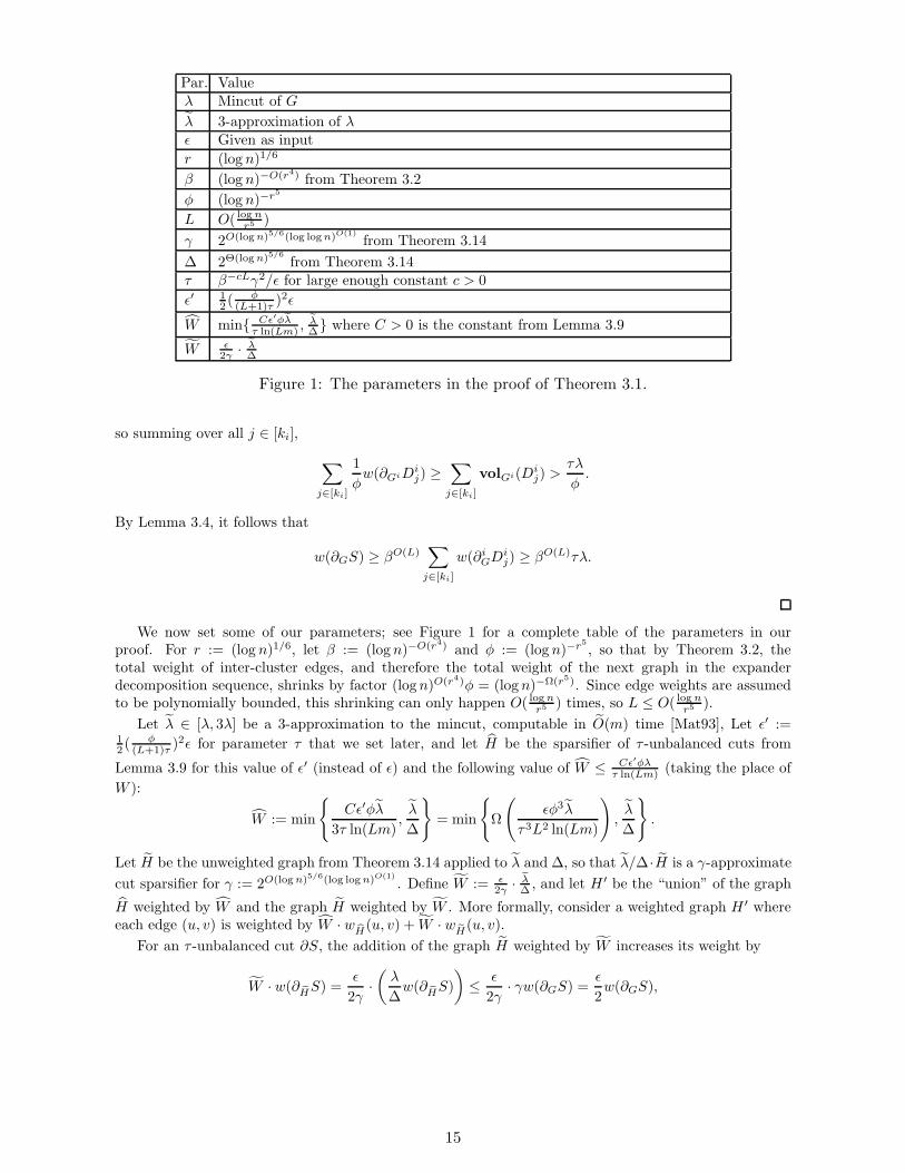
Figure 1: The parameters in the proof of Theorem 3.1.

so summing over all j ∈ [ki],

∑

j∈[ki]

1

φw(∂GiDi

j) ≥∑

j∈[ki]

volGi(Dij) >

τλ

φ.

By Lemma 3.4, it follows that

w(∂GS) ≥ βO(L)∑

j∈[ki]

w(∂iGDij) ≥ βO(L)τλ.

We now set some of our parameters; see Figure 1 for a complete table of the parameters in ourproof. For r := (log n)1/6, let β := (logn)−O(r4) and φ := (log n)−r5 , so that by Theorem 3.2, thetotal weight of inter-cluster edges, and therefore the total weight of the next graph in the expanderdecomposition sequence, shrinks by factor (logn)O(r4)φ = (logn)−Ω(r5). Since edge weights are assumedto be polynomially bounded, this shrinking can only happen O( log n

r5 ) times, so L ≤ O( log nr5 ).

Let λ ∈ [λ, 3λ] be a 3-approximation to the mincut, computable in O(m) time [Mat93], Let ǫ′ :=12 (

φ(L+1)τ )

2ǫ for parameter τ that we set later, and let H be the sparsifier of τ -unbalanced cuts from

Lemma 3.9 for this value of ǫ′ (instead of ǫ) and the following value of W ≤ Cǫ′φλτ ln(Lm) (taking the place of

W ):

W := min

Cǫ′φλ

3τ ln(Lm),λ

∆

= min

Ω

(ǫφ3λ

τ3L2 ln(Lm)

),λ

∆

.

Let H be the unweighted graph from Theorem 3.14 applied to λ and ∆, so that λ/∆·H is a γ-approximate

cut sparsifier for γ := 2O(logn)5/6(log logn)O(1)

. Define W := ǫ2γ · λ

∆ , and let H ′ be the “union” of the graph

H weighted by W and the graph H weighted by W . More formally, consider a weighted graph H ′ whereeach edge (u, v) is weighted by W · wH(u, v) + W · wH(u, v).

For an τ -unbalanced cut ∂S, the addition of the graph H weighted by W increases its weight by

W · w(∂HS) =ǫ

2γ·

(λ

∆w(∂HS)

)≤

ǫ

2γ· γw(∂GS) =

ǫ

2w(∂GS),

15

so that∣∣∣w(∂GS)−

(W · w(∂HS) + W · w(∂HS)

)∣∣∣ ≤∣∣w(∂GS)− W · w(∂HS)

∣∣+ W · w(∂HS∗)

≤

((L+ 1)τ

φ

)2

· ǫ′λ+ǫ

2w(∂GS)

=ǫλ

2+ǫ

2w(∂GS)

≤ ǫw(∂GS).

In particular, any τ -unbalanced cut satisfies

(1 − ǫ)λ ≤ W · w(∂HS) + W · w(∂HS) ≤ (1 + ǫ)λ. (19)

Next, we show that all balanced cuts have weight at least λ in the graph H weighted by W . This iswhere we finally set τ := β−cLγ2/ǫ for large enough constant c > 0. For a balanced cut S,

W · w(∂HS) =ǫ

2γ·

(λ

∆w(∂HS)

)≥

ǫ

2γ·

(1

γw(∂GS)

)Clm.3.15

≥ǫ

γ2· βO(L)τλ ≥ λ.

Moreover, by Claim 3.6 for this value of τ ≥ β−O(L), the mincut ∂S∗ is τ -unbalanced, and therefore hasweight at least (1− ǫ)λ in H ′ by (19).

Therefore, H ′ preserves the mincut up to factor ǫ and has mincut at least (1 − ǫ)λ. It remains to

make all edge weights the same on this sparsifier. Since W = ǫ2γ · λ

∆ and the only requirement for ∆ from

Theorem 3.14 is that ∆ ≥ 2O(logn)5/6 , we can increase or decrease ∆ by a constant factor until eitherW/W or W/W is an integer. Then, we can let W := minW , W and define the unweighted graph H sothat #H(u, v) = wH′ (u, v)/W for all u, v ∈ V . Therefore, our final weight W is

W = minW , W = min

Ω

(ǫφ3λ

τ3L2 ln(Lm)

),λ

∆,ǫ

2γ·λ

∆

≥ ǫ42−O(logn)5/6(log logn)O(1)

λ,

so we can set f(n) := 2O(logn)5/6(log log n)O(1)

, as desired.Finally, we bound the running time. The expander decomposition sequence (Theorem 3.2) takes time

m1+O(1/r) + O(m/φ2), the unbalanced case (Theorem 3.2) takes time O(L2m), and the balanced case

takes time 2O(logn)5/6(log logn)O(1)

m. Altogether, the total is 2O(logn)5/6(log logn)O(1)

m, which concludes theproof of Theorem 3.1.

3.3 Removing the Maximum Weight Assumption

Let f(n) = 2O(logn)5/6(log logn)O(1)

be the function from Theorem 3.1. In this section, we show how touse Theorem 3.1, which assumes that the maximum edge weight in G is at most ǫ4λ/f(n), to proveTheorem 1.5, which makes no assumption on edge weights.

First, we show that we can assume without loss of generality that the maximum edge weight in G is atmost 3λ. To see why, the algorithm can first compute a 3-approximation λ ∈ [λ, 3λ] to the mincut with

the O(m)-time (2 + ǫ)-approximation algorithm of Matula [Mat93], and for each edge in G with weight

more than λ, reduce its weight to λ. Let the resulting graph be G. We now claim the following:

Claim 3.16. Suppose an unweighted graph H and some weightW satisfy the two properties of Theorem 1.5for G. Then, they also satisfy the two properties of Theorem 1.5 for G.

Proof. The only cuts that change value between G and G are those with an edge of weight more than λ,which means their value must be greater than λ ≥ λ. In particular, since G and G have the same mincutsand the same mincut values, both properties of Theorem 1.5 also hold when the input graph is G.

For the rest of the proof, we work with G instead of G. Define W := ǫ4λ/(3f(n)), which satisfies

W ≤ ǫ4λ/f(n). For each edge e in G, split it into ⌈w(e)/W ⌉ parallel edges of weight at most W each,

whose sum of weights equals w(e); let the resulting graph be G. Apply Theorem 3.1 on G, which returns

16

an unweighted graph H and weight W ≥ ǫ4λ/f(n) such that the two properties of Theorem 1.5 hold for

G. Clearly, the cuts are the same in G and G: we have w(∂GS) = w(∂GS) for all S ⊆ V . Therefore, the

two properties also hold for G, as desired.We now bound the size of G′ and the running time. Since w(e) ≤ λ, we have ⌈w(e)/W ⌉ ≤ ⌈3f(n)/ǫ4⌉,

so each edge splits into at most O(f(n)/ǫ4) edges and the total number of edges is m ≤ O(f(n)/ǫ4) ·m.

Therefore, Theorem 3.1 takes time 2O(logn)5/6(log logn)O(1)

m = ǫ−42O(logn)5/6(log logn)O(1)

m, concluding theproof of Theorem 1.5.

Acknowledgements

I am indebted to Sivakanth Gopi, Janardhan Kulkarni, Jakub Tarnawski, and Sam Wong for their super-vision and encouragement on this project while I was a research intern at Microsoft Research, as well asproviding valuable feedback on the manuscript. I also thank Thatchaphol Saranurak for introducing meto the boundary-linked expander decomposition framework [GRST20].

References

[CGL+19] Julia Chuzhoy, Yu Gao, Jason Li, Danupon Nanongkai, Richard Peng, and Thatchaphol Sara-nurak. A deterministic algorithm for balanced cut with applications to dynamic connectivity,flows, and beyond. arXiv preprint arXiv:1910.08025, 2019.

[Gab95] Harold N Gabow. A matroid approach to finding edge connectivity and packing arborescences.Journal of Computer and System Sciences, 50(2):259–273, 1995.

[GH61] Ralph E Gomory and Tien Chung Hu. Multi-terminal network flows. Journal of the Societyfor Industrial and Applied Mathematics, 9(4):551–570, 1961.

[GR98] Andrew V Goldberg and Satish Rao. Beyond the flow decomposition barrier. Journal of theACM (JACM), 45(5):783–797, 1998.

[GRST20] Gramoz Goranci, Harald Racke, Thatchaphol Saranurak, and Zihan Tan. The expander hi-erarchy and its applications to dynamic graph algorithms. arXiv preprint arXiv:2005.02369,2020.

[GT88] Andrew V. Goldberg and Robert Endre Tarjan. A new approach to the maximum-flow problem.J. ACM, 35(4):921–940, 1988.

[HO92] Jianxiu Hao and James B Orlin. A faster algorithm for finding the minimum cut in a graph. InProceedings of the third annual ACM-SIAM symposium on Discrete algorithms, pages 165–174.Society for Industrial and Applied Mathematics, 1992.

[HRW17] Monika Henzinger, Satish Rao, and Di Wang. Local flow partitioning for faster edge con-nectivity. In Proceedings of the Twenty-Eighth Annual ACM-SIAM Symposium on DiscreteAlgorithms, SODA 2017, Barcelona, Spain, Hotel Porta Fira, January 16-19, pages 1919–1938,2017.

[Kar93] David R Karger. Global min-cuts in rnc, and other ramifications of a simple min-cut algorithm.In SODA, volume 93, pages 21–30, 1993.

[Kar00] David R. Karger. Minimum cuts in near-linear time. J. ACM, 47(1):46–76, 2000.[KS96] David R Karger and Clifford Stein. A new approach to the minimum cut problem. Journal of

the ACM (JACM), 43(4):601–640, 1996.[KT18] Ken-ichi Kawarabayashi and Mikkel Thorup. Deterministic edge connectivity in near-linear

time. Journal of the ACM (JACM), 66(1):1–50, 2018.[LP20] Jason Li and Debmalya Panigrahi. Deterministic min-cut in poly-logarithmic max-flows. In

FOCS, 2020.[LS20] Yang P Liu and Aaron Sidford. Faster divergence maximization for faster maximum flow.

arXiv preprint arXiv:2003.08929, 2020.[LS21] Jason Li and Thatchaphol Saranurak. Deterministic weighted expander decomposition in

almost-linear time, 2021.[Mat93] David W Matula. A linear time 2+ ε approximation algorithm for edge connectivity. In

Proceedings of the fourth annual ACM-SIAM Symposium on Discrete algorithms, pages 500–504, 1993.

[NI92a] Hiroshi Nagamochi and Toshihide Ibaraki. Computing edge-connectivity in multigraphs andcapacitated graphs. SIAM Journal on Discrete Mathematics, 5(1):54–66, 1992.

17

[NI92b] Hiroshi Nagamochi and Toshihide Ibaraki. A linear-time algorithm for finding a sparse k-connected spanning subgraph of a k-connected graph. Algorithmica, 7(5&6):583–596, 1992.

[Sar21] Thatchaphol Saranurak. A simple deterministic algorithm for edge connectivity. In Symposiumon Simplicity in Algorithms (SOSA), pages 80–85. SIAM, 2021.

[ST04] Daniel A. Spielman and Shang-Hua Teng. Nearly-linear time algorithms for graph partitioning,graph sparsification, and solving linear systems. In STOC, pages 81–90. ACM, 2004.

[SW97] Mechthild Stoer and FrankWagner. A simple min-cut algorithm. Journal of the ACM (JACM),44(4):585–591, 1997.

[SW19] Thatchaphol Saranurak and Di Wang. Expander decomposition and pruning: Faster, stronger,and simpler. In SODA, pages 2616–2635. SIAM, 2019.

A Boundary-Linked Expander Decomposition

In this section, we prove Theorem 3.2 assuming the subroutine WeightedBalCutPrune from [LS21]. Ourproof is directly modeled off of the proof of Corollary 6.1 of [CGL+19] and the proof of Theorem 4.5 of [GRST20],so we claim no novelty in this section.

We will work with weighted multigraphs with self-loops, and we re-define the degree deg(v) to meanw(∂(v)) plus the total weight of all self-loops at vertex v. All other definitions that depend on deg(v),such as vol(S) and Φ(G), are also affected.

Given a weighted graph G = (V,E), a parameter r > 0, and a subset A ⊆ V , define GAr as thegraph G[A] with the following self-loops attached: for each edge e ∈ E(A, V \ A) with endpoint v ∈ A,add a self-loop at v of weight r · w(e). The following observation is immediate by definition:

Observation A.1. For any graph G = (V,E) and subset A ⊆ V , Property (1) of Theorem 3.2 holds forVi = A iff G[A]β/φ is a φ-expander.

We now define the WeightedBalCutPrune problem from [LS21]5 and their algorithm.

Definition A.2 (WeightedBalCutPrune problem, Definition 2.3 of [LS21]). The input to the α-approximateWeightedBalCutPrune problem is a graph G = (V,E), a conductance parameter 0 < φ ≤ 1, and anapproximation factor α. The goal is to compute a cut (A,B) in G, with wG(A,B) ≤ αφ · vol(B), suchthat one of the following holds: either

1. (Cut) vol(A),vol(B) ≥ vol(V )/3; or2. (Prune) vol(A) ≥ vol(V )/2, and Φ(G[A]) ≥ φ.

Theorem A.3 (WeightedBalCutPrune algorithm, Theorem 2.4 of [LS21]). There is a deterministic algo-rithm that, given a graph G = (V,E) with m edges and polynomially bounded edge weights, and parameters

0 < ψ ≤ 1 and r ≥ 1, solves the (logn)O(r4)-approximate WeightedBalCutPrune problem in timem1+O(1/r).

The (Prune) case requires the additional trimming step described in the lemma below. While[GRST20] prove it for unweighted graphs only, the algorithm translates directly to the weighted case;6

see, for example, Theorem 4.2 of [SW19].

Lemma A.4 (Trimming, Lemmas 4.9 and 4.10 of [GRST20]). Given a weighted graph G = (V,E) andsubset A ⊆ V such that GA is an 8φ-expander and w(EG(A, V \ A)) ≤ φ

16volG(A), we can compute a

“pruned” set P ⊆ A in deterministic O(m/φ2) time with the following properties:1. volG(P ) ≤

4φw(EG(A, V \A)),

2. w(EG(A′, V \A′)) ≤ 2w(EG(A, V \A)) where A′ := A \ P , and

3. GA′1/(8φ) is a φ-expander.

We now prove Theorem 3.2 assuming Theorem A.3. Our proof is copied almost ad verbatim from theproof of Corollary 6.1 of [CGL+19] on expander decompositions, with the necessary changes to prove theadditional boundary-linked property.

We maintain a collection H of vertex-disjoint graphs that we call clusters, which are subgraphs of Gwith some additional self-loops. The set H of clusters is partitioned into two subsets, set HA of activeclusters, and set HI of inactive clusters. We ensure that each inactive cluster H ∈ HI is a φ-expander.

5Their definition is more general and takes in a demand vector d ∈ RV on the vertices; we are simply restricting ourselvesto d(v) = deg(v) for all v ∈ V , which gives our definition.

6In particular, the core subroutine, called Unit-Flow in [SW19], is based on the push-relabel max-flow algorithm, whichworks on both unweighted and weighted graphs.

18

We also maintain a set E′ of “deleted” edges, that are not contained in any cluster in H. At the beginningof the algorithm, we let H = HA = G, HI = ∅, and E′ = ∅. The algorithm proceeds as long as HA 6= ∅,

and consists of iterations. Let α = (logn)O(r4) be the approximation factor from Theorem A.3.In every iteration, we apply the algorithm from Theorem A.3 to every graph H ∈ HA, with the same

parameters α, r, and φ. Let U be the vertices of H . Consider the cut (A,B) in H that the algorithmreturns, with

w(EH(A,B)) ≤ αφ · vol(U) ≤ǫ · vol(U)

c logn. (20)

We add the edges of EH(A,B) to set E′.

If volH(B) ≥ vol(U)32α , then we replace H with HA1/(α

2φ log n) and HB1/(α2φ logn) in H and in HA.

Note that the self-loops add a total volume of

1

α2φ log n· w(EH (A,B)) ≤

1

α2φ logn· αφvol(U) =

1

α lognvol(U). (21)

Otherwise, if volH(B) < vol(U)32α ≤ vol(U)/3, then we must be in the (Prune) case, which means that

volH(A) ≥ vol(U)/2 and graph HA1/(8φ) has conductance at least φ. Since

w(EH (A,B)) ≤ αφ · volH(B) ≤φ

32vol(U) ≤

φ

16vol(A),

we can call Lemma A.4 on A to obtain a pruned set P ⊆ A such that

volH(P ) ≤4

φw(EH (A,B)) ≤

1

8vol(U)

and

w(EH(A′, U \A′)) ≤ 2w(EH(A,B)) ≤φ

8vol(A)

for A′ := A \P , and HA′1/(8φ) is a φ-expander. Add the edges of EH(A′, U \A′) to E′, remove H fromH and HA, add HA′1/(8φ) to H and HI , and add HB ∪ P1/(8φ) to H and HA. Observe that

volH(B ∪ P ) = volH(B) + volH(P ) ≤1

2volH(U) +

1

8volH(U) ≤

5

8vol(U).

When the algorithm terminates, HA = ∅, and so every graph in H has conductance at least φ. Noticethat in every iteration, the maximum volume of a graph in HA is at most a factor (1 − 1

32α ) of what itwas before. Since edge weights are polynomially bounded, the number of iterations is at most O(α log n).On each iteration, the total volume of graphs in HA increases by at most factor 1 + 2

α logn factor due to

the self-loops added in (21), so the total volume of all H ∈ H at the end is at most a constant factor ofthe initial volume volG(V ).

The output of the algorithm is the partition of V induced by the vertex sets of H ∈ H, so the inter-cluster edges is a subset of E′. It is easy to verify by (20) that the total weight of edges added to set E′

in every iteration is at most αφ times the total volume of graphs in HA at the beginning of that iteration,which is O(volG(V )). Over all O(α logn) iterations, the total weight of E′ is O(α logn) · αφvolG(V ) ≤

(log n)O(r4)φvolG(V ), fulfilling property (2) of a boundary-linked expander decomposition.It remains to show that for each graph H ∈ HI , its vertex set U satisfies the boundary-linked φ-

expander property (1) of Theorem 3.2. For each boundary edge e ∈ EG(U, V \ U), it was created at

some iteration where we either added 1α2φ log n self-loops or 1

8φ self-loops, so G[U ]min1/(α2φ logn),1/(8φ)

is a subgraph of H . Since H is a φ-expander, so is G[U ]min1/(α2φ logn),1/(8φ), and property (1) forβ := min1/α2, 1/8 follows by Observation A.1.

It remains to analyze the running time of the algorithm. The running time of a single iteration isbounded by O(m1+O(1/r)) + O(m/φ2). Since the total number of iterations is bounded by O(log n), thetotal running time is the same, asymptotically.

19

B Lossy Unweighted Sparsifier

In this section, we prove Theorem 3.14, restated below.

Theorem 3.14. Let G be an weighted multigraph with mincut λ whose edges have weight at most O(λ).

For any parameters λ ∈ [λ, 3λ] and ∆ ≥ 2O(logn)5/6 , we can compute, in deterministic 2O(logn)5/6(log logn)O(1)

m+O(∆m) time, an unweighted multigraph H such that W ·H is a γ-approximate cut sparsifier of G, where

γ ≤ 2O(logn)5/6(log logn)O(1)

and W = λ/∆. (The graph H does not need to be a subgraph of G.) Moreover,the algorithm does not need to know the mincut value λ.

We will work with weighted multigraphs with self-loops, and we re-define the degree deg(v) to meanw(∂(v)) plus the total weight of all self-loops at vertex v. All other definitions that depend on deg(v),such as vol(S) and Φ(G), are also affected.

The construction of the sparsifier H is recursive. The original input is graph G = G0, and let theinput graph on level i ≥ 0 of the recursion be Gi, with U i as its vertex set. Let U i

1, Ui2, . . . be an expander

decomposition of Gi, and let Gi+1 be the graph with each set U ij contracted to a single vertex ui+1

j . If Gi+1

has more than one vertex, recursively compute a sparsifier on Gi+1, which still has mincut at least λ, andlet the sparsifier beHi+1. For each edge (ui+1

j , ui+1k ) inHi+1, we select a vertex x ∈ U i

j and y ∈ U ik and add

edge (x, y) to an initially empty graphHi0 on U

i. We do this in a way that each vertex v ∈ U i is incident to

at most

⌈degHi+1(ui+1

j ) ·w(EGi (v,U

i\Uij ))

degGi+1(ui+1j )

⌉many edges. Since

∑v∈Ui

jw(EGi(v, U i \U i

j)) = degGi+1(ui+1j ),

this is always possible by an averaging argument. Next, for each cluster U ij , we compute an Ω(1)-expander

multigraph Hij (possibly with self-loops) on the vertices U i

j such that for all v ∈ U ij ,

degGi(v) ≤W · degHij(v) ≤ 9 degGi(v). (22)

This can be done by using the lemma below with d(v) = degGi(v)/W ≥ λ/W ≥ 1. The running time isat most O(

∑v∈Ui

degGi(v)/W ) ≤ O(∑

e∈E w(e)/W ), which is O(mλ/W ) = O(∆m) since by assumption,

all edges in G have weight at most O(λ), and W = λ/∆ = Θ(λ/∆).

Lemma B.1. Given a vertex set V and real numbers d(v) ≥ 1 : v ∈ V , there exists a universal constantC0 such that we can construct, in O(

∑v∈V d(v)) time, an Ω(1)-expander multigraph H on V (possibly

with self-loops) such that for all v ∈ V ,

d(v) ≤ degH(v) ≤ 9d(v).

Proof. We use the following theorem of [CGL+19]:

Theorem B.2. There is a constant α0 > 0 and a deterministic algorithm that, given an integer n > 1,in time O(n) constructs a graph Hn with |V (Hn)| = n, such that Hn is an α0-expander, and every vertexin Hn has degree at most 9.

Let n =∑

v∈V d(v), and let Hn be the constructed graph on vertex set Vn. Partition Vn arbitrarilyinto subsets Uv : v ∈ V such that |Uv| = d(v) for each v ∈ V . Let H be the graph Hn with each set Uv

contracted to a single vertex v, keeping self-loops, so that degH(v) = volHn(Uv). It is not hard to seethat expansion does not decrease upon contraction, so H is still an Ω(1)-expander. We can bound thedegrees degH(v) as

d(v) = |Uv| ≤ volHn(Uv) = degH(v) = volHn(Uv) ≤ 9|Uv| = 9d(v).

The final sparsifier Hi is Hi0 ∪H

i1 ∪ H

i2 ∪ · · · . This concludes the construction of sparsifier Hi. (We

keep the self-loops, even though they serve no purpose for the sparsifier’s guarantees, because we findthat including them simplifies the analysis.) Note that this recursive algorithm implicitly constructs anexpander sequence G0, G1, G2, . . . , GL of G over its recursive calls.

Fix a subset ∅ ( S ( U i, let Si be the canonical decomposition sequence of S, and letDij be constructed

as before, so that they satisfy (7) and (8) for all i, j.

Claim B.3. For all i and all v ∈ U i,

degGi(v) ≤W · degHi(v) ≤ 10(L+ 1) · degGi(v).

20

Proof. We prove the stronger statement

degGi(v) ≤W · degHi(v) ≤ 10(L+ 1− i) · degGi(v)

by induction from i = L down to 0. For i = L, since it is the last level, the entire graph GL is a singlecluster. By construction, HL consists only of a single constant-expander HL

1 that satisfies degGL(v) ≤W · degHL

1(v) ≤ 9 degGL(v), which completes the base case of the induction.

For i < L, by induction, we have W · degHi+1(v) ≤ 10(L− i) · degGi+1(v). Fix a cluster U ij that gets

contracted to vertex ui+1j in Gi+1, and fix a vertex v ∈ U i

j . For the graph Hi0, we have

degHi0(v) ≤

⌈degHi+1 (ui+1

j ) ·w(EGi (v, U i \ U i

j))

degGi+1(ui+1j )

⌉≤ 1 + degHi+1(ui+1

j ) ·w(EGi(v, U i \ U i

j))

degGi+1(ui+1j )

≤ 1 +10(L− i)

Ww(EGi(v, U i \ U i

j)) (23)

≤ 1 +10(L− i)

WdegGi(v).

For the graph Hij , by construction (22), we have

degGi(v) ≤W · degHij(v) ≤ 9 degGi(v).

Therefore,

W · degHi(v) =W ·(degHi

0(v) + degHi

j(v))≥W · degHi

j(v) ≥ degGi(v)

andW · degHi (v) =W ·

(degHi

0(v) + degHi

j(v))≤W + 10(L− i) degGi(v) + 9 degGi(v).

We can assume that ∆ ≥ 3, so that degGi(v) ≥ λ ≥ λ/3 = ∆W/3 ≥W , and the above is at most

degGi(v) + 10(L− i) degGi(v) + 9 degGi(v) = 10(L+ 1− i) · degGi(v),

which completes the induction.

Claim B.4 (Analogue of (7) for Hi). For all i, j,

w(∂Hi [Uij ]Di

j)

volHi[Uij ](Di

j)≥ Ω

(φ

β

).

Proof. Note that Hi[U ij ] is exactly H

ij by construction. We begin by bounding volumes in Gi.

volGi(Dij) = volGi[Ui

j ](Di

j) + w(EGi (Dij , U

i \ U ij))

≤ volGi[Uij ](Di

j) +β

φw(EGi(Di

j , Ui \ U i

j))

(6)≤ volGi(U i

j \Dij) +

β

φw(EGi(Di

j , Ui \ U i

j))

≤β

φ

(volGi(U i

j \Dij) + w(EGi(Di

j , Ui \ U i

j))

=β

φvolGi(U i

j \Dij).

We now translate this volume bound to Hij . By the construction of Hi

j (22),

volHij(Di

j) ≤9volGi(Di

j)

W≤

9βvolGi(U ij \D

ij)

Wφ≤

9βvolHij(U i

j \Dij)

φ. (24)

Since Hij is an Ω(1)-expander,

w(∂Hij(Di

j)) ≥ Ω(1) ·minvolHij(Di

j),volHij(U i

j \Dij) ≥ Ω(1) ·

φ

9βvolHi

j(Di

j),

as desired.

21

Claim B.5 (Analogue of (8) for Hi). For all i < L and j,

w(∂Hi [Uij ]Di

j)

w(EHi (Dij , U

i \ U ij))

≥ Ω

(1

L

).

Proof. Let ui+1j ∈ U i+1 be the vertex that the cluster U i

j contracts to in Gi+1. Again, note that Hi[U ij ]

is exactly Hij by construction.

The only edges of EHi (Dij , U

i \ U ij) belong to Hi

0, so

EHi (Dij , U

i \ U ij) = EHi

0(Di

j , Ui \ U i

j) =∑

v∈Dij

degHi0(v)

(23)≤

∑

v∈Dij

(1 +

10(L− i)

Ww(EGi(v, U i \ U i

j))

)

≤∑

v∈Dij

(1 +

10L

Ww(EGi(v, U i \ U i

j))

)

= |Dij |+

10L

Ww(EGi (Di

j , Ui \ U i

j)).

We upper bound the term w(EGi(Dij , U

i \ U ij)) in two ways:

β

φw(EGi(Di

j , Ui \ U i

j)) ≤ volGi[Uij ](Di

j) +β

φw(EGi(Di

j , Ui \ U i

j))

≤β

φ

(volGi[Ui

j ](Di

j) + w(EGi (Dij , U

i \ U ij)))

=β

φvolGi(Di

j);

β

φw(EGi(Di

j , Ui \ U i

j)) ≤ volGi[Uij ](Di

j) +β

φw(EGi(Di

j , Ui \ U i

j))

(6)≤ volGi[Ui

j ](U i

j \Dij) +

β

φw(EGi(Di

j , Ui \ U i

j))

≤β

φ

(volGi[Ui

j ](U i

j \Dij) + w(EGi (Di

j , Ui \ U i

j))

=β

φvolGi(U i

j \Dij).

Therefore,

EHi (Dij , U

i \ U ij) ≤ |Di

j |+10L

WminvolGi(Di

j),volGi(U ij \D

ij)

(22)≤ |Di

j |+ 10LminvolHij(Di

j),volHij(U i

j \Dij) .

We now bound |Dij | as follows. By construction (22), for all v ∈ U i

j ,

degHij(v) ≥

degGi(v)

W≥

λ

W≥

λ

3W=

∆

3,

which means that

|Dij | ≤

volHij(Di

j)

∆/3

(24)≤

27βvolHij(U i

j \Dij)

∆φ≤ volHi

j(U i

j \Dij)

as long as we impose the condition

∆ ≥27β

φ. (25)

Therefore,|Di

j | ≤ minvolHij(Di

j),volHij(U i

j \Dij)

22

andw(EHi (Di

j , Ui \ U i

j)) ≤ (10L+ 1)minvolHij(Di

j),volHij(U i

j \Dij).

Since Hij is an Ω(1)-expander,

w(∂HijDi

j) ≥ Ω(1) ·minvolHij(Di

j),volHij(U i

j \Dij) ≥ Ω

(1

L

)· w(EHi (Di

j , Ui \ U i

j)),

as desired.

Lemma B.6. For all i, j,

Ω

(φ

β

)w(∂GiDi

j) ≤W · w(∂HiDij) ≤ O

(L

φ

)w(∂GiDi

j).

Proof. For the lower bound, we have

w(∂HiDij) ≥ w(∂Hi [Ui

j ]Di

j)Clm.B.4

≥ Ω

(φ

β

)volHi[Ui

j ](Di

j)

(22)≥ Ω

(φ

β

)·1

WvolGi(Di

j)

≥ Ω

(φ

β

)·1

Ww(∂GiDi

j).

For the upper bound,

w(∂HiDij) = w(∂Hi [Ui

j ]Di

j) + w(EHi (Dij , U

i \ U ij))Clm.B.5

≤ (1 + O(L)) · w(∂Hi [Uij ]Di

j)

≤ (1 + O(L)) · volHi [Uij ](Di

j)

(22)≤ (1 + O(L)) ·

9

WvolGi(Di

j)

≤ (1 + O(L)) ·9

W

(volGi[Ui

j ](Di

j) + w(EGi(Dij , U

i \ U ij)))

≤ (1 + O(L)) ·9

W

(1

φw(∂Gi[Ui

j ]Di

j) + w(EGi(Dij , U

i \ U ij))

)

≤ (1 + O(L)) ·9

W·1

φ

(w(∂Gi[Ui

j ]Di

j) + w(EGi(Dij , U

i \ U ij)))

= (1 + O(L)) ·9

W·1

φw(∂GiDi

j).

Lemma B.7. W ·H is a γ-approximate sparsifier with γ = maxO(β−O(L)L/φ), O(LO(L)β/φ)

.

Proof. Since Claim B.5 is an analogue of (8) for graph H with the parameter β replaced by Ω(1/L), wecan apply Lemmas 3.3 and 3.4 to H , obtaining

w(∂HS) ≤L∑

i=0

∑

j∈[ki]

w(∂HiDij) ≤ LO(L)w(∂HS).

Combining this with Lemma B.6,

w(∂HS) ≤L∑

i=0

∑

j∈[ki]

w(∂HiDij) ≤ (1 +O(L)) ·

9

W·1

φ

L∑

i=0

∑

j∈[ki]

w(∂GiDij)

Lem.3.4≤ (1 +O(L)) ·

9

W·1

φ· β−O(L)w(∂GS)

23

and

w(∂HS) ≥ L−O(L)L∑

i=0

∑

j∈[ki]

w(∂HiDij) ≥ L−O(L) ·

L∑

i=0

∑

j∈[ki]

Ω

(φ

β

)1

Ww(∂GiDi

j)

Lem.3.3≥ L−O(L) · Ω

(φ

β

)1

Ww(∂GS).

Finally, we set the parameters r ≥ 1, β, L, φ. For r := (logn)1/6, let β := (log n)−O(r4) and φ :=

(log n)−r5 , so that by Theorem 3.2, the total weight of inter-cluster edges, and therefore the total weight

of the next graph in the expander decomposition sequence, shrinks by factor (logn)O(r4)φ = (logn)−Ω(r5).Since edge weights are assumed to be polynomially bounded, this shrinking can only happen O( log n

r5 )

times, so L ≤ O( log nr5 ). Therefore, our approximation factor is

γ = maxO(β−O(L)L/φ), O(LO(L)β/φ)

= O(β−O(L)L/φ) = 2O(logn)5/6(log log n)O(1)

,

and the running time, which is dominated by the output size O(∆m) and the calls to Theorem 3.2 andLemma A.4, is

O(∆m) +m1+O(1/r) + O(m/φ2) = 2O(logn)5/6(log logn)O(1)

m+O(∆m).

Finally, the condition ∆ ≥ 27βφ from (25) becomes ∆ ≥ 2Ω(logn)5/6 , concluding the proof of Theorem 3.14.

24