Care to Wager Again? An Appraisal of PaulEhrlich’s Counterbet Offer to Julian Simon,Part 2: Critical Analysis

Pierre Desrochers, University of Toronto

Vincent Geloso, King’s University College

Joanna Szurmak, University of Toronto

Objective. This paper provides the first comprehensive assessment of the outcome of Paul Ehrlich’sand Stephen Schneider’s counteroffer (1995) to economist Julian Simon following Ehrlich’s loss inthe famous Ehrlich-Simon wager on economic growth and the price of natural resources (1980-1990). Our main conclusion in a previous article is that, for indicators that can be measured satis-factorily or can be inferred from proxies, the outcome favors Ehrlich-Schneider in the first decadefollowing their offer. This second article extends the timeline towards the present time period to ex-amine the long-term trends of each indicator and proxy, and assesses the reasons invoked by Simonto refuse the bet. Methods. Literature review, data gathering, and critical assessment of the indi-cators and proxies suggested or implied by Ehrlich and Schneider. Critical assessment of Simon’sreasons for rejecting the bet. Data gathering for his alternative indicators. Results. For indicatorsthat can be measured directly, the balance of the outcomes favors the Ehrlich-Schneider claimsfor the initial ten-year period. Extending the timeline and accounting for the measurement limita-tions or dubious relevance of many of their indicators, however, shifts the balance of the evidencetowards Simon’s perspective. Conclusion. The fact that Ehrlich and Schneider’s own choice of indi-cators yielded mixed results in the long run, coupled with the fact that Simon’s preferred indicatorsof direct human welfare yielded largely favorable outcomes is, in our opinion, sufficient to claimthat Simon’s optimistic perspective was largely validated.

In 1995, eco-pessimist Stanford biology professors Paul R. Ehrlich and Stephen Schnei-der offered optimist economist Julian Simon a 10-year wager based on a set of “indirectmeasures” of environmental conditions and human health indicators. Simon declined theproposal, claiming it lacked direct and objectively measurable connections to human wel-fare. Ehrlich and his supporters have since used Simon’s rejection of their offer as a way toundermine his analysis. Part 1 of this article provided the first comprehensive assessmentof the outcome of the Ehrlich-Schneider wager. Its conclusion was that, for indicators thatcan be measured satisfactorily or can be inferred from (more or less adequate) proxies, theoutcome favored Ehrlich and Schneider’s perspective. In this follow-up article, we extendthe timeline of Ehrlich and Schneider’s indicators and proxies toward the present time pe-riod, discuss in more detail their limitations and problems with their interpretation, andassess Julian Simon’s proposed alternatives to this wager. In doing so, we suggest that theevidence shifts toward Simon’s perspective.

Direct correspondence to Pierre Desrochers, Department of Geography, Geomatics and Environment,University of Toronto Mississauga, Mississauga, ON, Canada L5L 1C6 〈pierre.desrochers@utoronto.ca〉.SOCIAL SCIENCE QUARTERLYC© 2021 by the Southwestern Social Science AssociationDOI: 10.1111/ssqu.12920

2 Social Science Quarterly

In Part 1 of this two-paper set, we analyzed the outcomes of the 1995 wager offered tothe optimist economist Julian Simon by the eco-pessimist Stanford biology professors PaulR. Ehrlich and Stephen Schneider. Unlike Simon, who had left the choice of commoditiesand time period to his opponents in the famous 1980 bet, Ehrlich and Schneider selectedall the indirect measures of environmental conditions, human health indicators, and timeperiod (Table 1).

Simon declined their proposal, claiming it lacked direct and objectively measurable con-nections to human welfare. He also suggested a few alternatives that, he argued, met thiscriterion. Ehrlich and his supporters have since used Simon’s rejection of their offer toundermine his broader analysis of the environmental impact of population and economicgrowth.

Our assessment in Part 1 of this article set was that, on Ehrlich and Schneider’s terms,Simon would have lost the bet by a wide margin. In this Part 2, we probe deeper intothe counterwager by extending the timeline of indirect measures and proxies toward thepresent time period, discussing in more detail their limitations, and assessing Julian Simon’ssuggested alternative indicators. In doing so, we suggest that the balance of the evidenceshifts the outcome toward Simon’s perspective.

Extension of the Time Frame and Assessment of Indicators

Outcomes 1–5: Temperature and Atmosphere

Extending the time horizon for claims related to the global average temperature and theatmospheric concentrations of various molecules does change the results somewhat. Claims1 (global average temperature), 2 (atmospheric carbon dioxide), and 3 (atmospheric ni-trous oxide) remain consistent with Ehrlich and Schneider’s predicted trends (Tans andKeeling, n.d.; Environmental Protection Agency (EPA), 2016; World Meteorological Or-ganization, 2014; Medhaug et al., 2017; Met Office Hadley Centre, 2020; NOAA CDR,2020; NOAA ESRL, 2020; NOAA GISS, 2020). Extending the time horizon for tropo-spheric ozone (claim 4) and sulfur dioxide (claim 5) however, indicates or strongly suggestsa trend reversal. With regard to tropospheric ozone, many observation posts discussed inGaudel et al.’s (2018) exhaustive assessment of ozone concentration suggest improvementssince 2000. It is hard to assess whether levels observed for 2014 by Gaudel et al. (2018)were globally below those for 1994, but tropospheric ozone concentrations show decreasingtrends since 2000. By 2015, sulfur dioxide concentrations were significantly below thoseobserved in 1995 on a global scale and began falling in East Asia in 2005 (Aas et al., 2019).

Outcomes 6, 7, and 8: Agricultural Land and Commodities

An extension of the time window to include the most recent data points does not changethe trend with regard to per capita agricultural land (claims 6 and 7 on fertile cropland andagricultural soil per person), as the quantity of land under cultivation remained stable whilepopulation increased (FAO, 2020a; United Nations, 2016). The extension of the timewindow, however, gives Simon a win with regard to rice and wheat per person (claim 8)which, by 2016–2018, were, respectively, 5.91 percent above and virtually equal (0.0002percent above) to their 1992–1994 levels (FAO, 2020a).

APPRAISAL OF EHRLICH’S COUNTERBET TO SIMON PART 2 3

TAB

LE1

Term

sof

the

Ehr

lich–

Sch

neid

erC

ount

erw

ager

1.Th

eth

ree

year

s20

02–2

004

will

onav

erag

eb

ew

arm

erth

an19

92–1

994.

2.Th

ere

will

be

mor

eca

rbon

dio

xid

ein

the

atm

osp

here

in20

04th

anin

1994

.3.

Ther

ew

illb

em

ore

nitro

usox

ide

inth

eat

mos

phe

rein

2004

than

in19

94.

4.Th

eco

ncen

trat

ion

ofoz

one

inth

elo

wer

atm

osp

here

(the

trop

osp

here

)w

illb

eg

reat

erin

2004

than

in19

94.

5.E

mis

sion

sof

the

air

pol

luta

ntsu

lfur

dio

xid

ein

Asi

aw

illb

esi

gni

fican

tlyg

reat

erin

2004

than

in19

94.

6.Th

ere

will

be

less

fert

ilecr

opla

ndp

erp

erso

nin

2004

than

in19

94.

7.Th

ere

will

be

less

agric

ultu

rals

oilp

erp

erso

nin

2004

than

in19

94.

8.Th

ere

will

be

onav

erag

ele

ssric

ean

dw

heat

gro

wn

per

per

son

in20

02–2

004

than

in19

92–1

994.

9.In

dev

elop

ing

natio

nsth

ere

will

be

less

firew

ood

avai

lab

lep

erp

erso

nin

2004

than

in19

94.

10.T

here

mai

ning

area

ofvi

rgin

trop

ical

moi

stfo

rest

sw

illb

esi

gni

fican

tlysm

alle

rin

2004

than

in19

94.

11.T

heoc

eani

cfis

herie

sha

rves

tper

per

son

will

cont

inue

itsd

ownw

ard

trend

and

thus

in20

04w

illb

esm

alle

rtha

nin

1994

.12

.The

rew

illb

efe

wer

pla

ntan

dan

imal

spec

ies

still

exta

ntin

2004

than

in19

94.

13.M

ore

peo

ple

will

die

ofA

IDS

in20

04th

and

idin

1994

.14

.Bet

wee

n19

94an

d20

04,s

per

mco

unts

ofhu

man

mal

esw

illco

ntin

ueto

dec

line

and

rep

rod

uctiv

ed

isor

der

sw

illco

ntin

ueto

incr

ease

.15

.The

gap

inw

ealth

bet

wee

nth

eric

hest

10p

erce

ntof

hum

anity

and

the

poo

rest

10p

erce

ntw

illb

eg

reat

erin

2004

than

in19

94.

SO

UR

CE:E

hrlic

han

dE

hrlic

h(1

996:

100-

104)

.

4 Social Science Quarterly

TABLE 2

Food Supply Per Capita, 1994–2017

Data set 2017 2004 1994

FAOSTAT, world(kcal sup-ply/capita/day)

2,913 2,751 2,640

FAOSTAT, leastdevelopedcountries(kcal sup-ply/capita/day)

2,422 2,189 1,958

SOURCE: FAO (2020).

The most obvious criticism of Ehrlich and Schneider’s choice of indicators is that in1994 all advanced economies had less soil available per capita than a century before, yetfood per capita had never been so abundant. Indeed, economic historians have docu-mented improved yields per unit of agricultural land going back at least to the middleof the 19th century (Federico, 2008). Furthermore, one should not assume that decliningavailability of a particular commodity per capita signals greater scarcity rather than chang-ing consumer tastes. For instance, out of the 71 foodstuffs tracked by the FAO for theperiod 1994–2004, the supply declined for 15, remained stable for 15, and increased for38 (FAO, 2020a). In the period 1994–2011, the supply increased for 47 of these items.Worldwide, positive trends can be seen in the quantities of calories supplied per day perperson over the 1994−2017 period, for both the world as a whole and in the least devel-oped countries (Table 2).

Ehrlich and Schneider’s claim that “less fertile cropland per person” and “less agricul-tural soil per person” are indicative of a crisis must ultimately be rooted in their beliefin decreasing returns, a position consistent with their catastrophist outlook. Yet, theavailable evidence convincingly suggests long-standing increasing returns in agriculturalproduction. Indeed, for the period of the counteroffer, the food supply has increasedmore rapidly than population, thus providing more calories per capita, while the quantityof land used to produce foodstuffs has remained virtually unchanged (Deaton, 2013).The History Database of the Global Environment (Klein Goldewjik et al., 2011) furthersuggests that agricultural land use per capita peaked in 3000 BCE, fell rapidly to the yearzero, remained more or less stable thereafter until 1940. From 1940 to 2016, hectares percapita fell from 1.55 to 0.66 while the food supply grew rapidly.

Recent projections to 2050 by Ausubel, Wernick, and Waggoner (2013) further suggesta decline in the absolute amount of farmland needed to feed a larger population, a situationthey labeled “peak farmland” that further allows considerable rewilding of much marginalagricultural lands (Ausubel, 2015). Alexandratos and Bruinsma (2012) are less optimisticthan Ausubel et al. (2015) and project instead that arable land will increase to 2030 andstabilize thereafter to 2050. Others, such as Folberth et al. (2020), have devised ways ofusing high-yield agricultural practices to reduce current agricultural land use by 50 percent,including 40 percent in biodiversity hotspots. By definition, if peak farmland is reached,Ehrlich and Schneider would win in perpetuity with a growing or stable population eventhough this outcome would actually vindicate Simon’s outlook.

APPRAISAL OF EHRLICH’S COUNTERBET TO SIMON PART 2 5

Outcomes 9 and 10: Firewood and Virgin Forests

Extending the time window does not change the outcome on firewood per person inless developed countries (claim 9), for there has indeed been a decline in firewood produc-tion per capita in those regions and in “woodfuel ‘hotspots’ [… where] nearly 300 millionpeople live with acute woodfuel scarcity” (Bailis et al., 2017:2). Reduced consumptionof wood fuel, however, is not necessarily problematic for both humanity and the envi-ronment as long as it is associated with increased prosperity and a fuel transition up the“energy ladder” from polluting biomass fuels (e.g., animal dung, crop residues, wood),which are inconvenient, inefficient, and severely harmful to human health (Bruce, Perez-Padilla, and Albalak, 2000). Various authorities in developing nations have long tried toreduce pressures on forests caused by subsistence-scale firewood procurement (World Re-sources Institute, 2003). Typically, however, a transition to more efficient and less pollutingenergy sources such as carbon fuels occurs spontaneously with greater material affluence(Goklany, 2009). Until, or whether, such a transition occurs in the world’s poorest regions,the demand for fuelwood is expected to increase with increasing population and income(FAO, 2010).

It seems legitimate to ask why Ehrlich and Schneider did not assume, or at least makeallowances for, the fact that growing affluence in the developing world would facilitate ben-eficial energy choices and transitions. Indeed, FAO (2010) acknowledged that the overallexploitation of forests worldwide has shifted from production to conservation, reaffirm-ing Simon’ prediction that prosperity and innovation would extend and ultimately sparenatural resources.

Using the proxy of tropical forest area loss since the 1990s does hand the long-termwin for claim 10 to Ehrlich and Schneider on the remaining area of virgin tropical moistforests. As Song et al. (2018:639) stated, however, “contrary to the prevailing view thatforest area has declined globally—tree cover has increased by 2.24 million km2 (+7.1%relative to the 1982 level). This overall net gain is the result of a net loss in the tropics beingoutweighed by a net gain in the extratropics.” Thus, the long-term trend for the “virgin”moist forest area is that of a moderate decline in the tropical areas, including the Amazon,but a decline that has been outweighed by afforestation in other areas of the world.

Furthermore, Ehrlich and Schneider’s concept of “virgin” tropical moist forests is highlycontentious in light of recent scholarship that documents past human disturbances ofecosystems once considered untouched by human activities (Williams, 2008; Hecken-berger and Neves, 2009; Levis et al., 2017; Lombardo et al., 2020). In the words ofbotanist Knut Faegri (1988:1–2), apart from “some small and doubtful exceptions, allvegetation types were created or modified by man.”

Much of the Amazon basin is thus now considered to be the recent rewilding of oncemassive orchards made up of hundreds of different crops of fruit, and palm and nut treesdomesticated, planted and maintained by significant indigenous populations decimated byEuropean diseases and conquest a few centuries ago. Indigenous Amazonian agricultural-ists profoundly altered local tree compositions and densities but also their genetic makeup(Heckenberger and Neves, 2009). The development of domesticated tree varieties paral-leled the transformation of wild wheat varieties into domesticated ones (Heckenberger andNeves, 2009). Native agriculturalists also created the so-called fertile Amazonian (anthro-pogenic) Dark Earths (Golinska, 2014; Heckenberger et al., 2008) that allowed “gardencity” agriculture to flourish (Heckenberger et al., 2008). The lead author of another re-cent Amazonian study thus declared: “This is Amazonia, this is one of these places thata few years ago we thought to be like a virgin forest, an untouched environment. Now

6 Social Science Quarterly

we’re finding this evidence that people were living there 10,500 years ago, and they startedpractising cultivation” (quoted in McGrath, 2020). “The ‘natural’ landscapes of precedinggenerations,” Faegri (1988:1–2) explained, “are now understood for what they really are:relics of earlier types of land-use […] By abandoning these methods and discontinuingtraditional land-use, the landscape was left to regenerate in response to other uses or non-use.” In other words, the notion of “virgin” forest in most parts of the world, particularlyin the Amazon, has been shown to be inaccurate.

Ehrlich and Schneider’s professed rationale for including the reduction in virgin trop-ical moist forest area was these forests’ function as a repository of genetic material forpharmaceutical research. “Biodiversity prospecting” is the practice of broadly surveying ge-netic and biochemical materials for potential commercial value (Simpson, 1997:12). Themarginal value, or the incremental benefit, of additional species would be high if there wereno substitutes for their biochemical properties (Craft and Simpson, 2001; Simpson, 1997).In nature, however, many species are capable of producing similar chemical compounds:“[S]pecies are very likely to prove redundant when there are large numbers from which tochoose for testing” (Simpson, 1997:13). Commercial pharmaceutical research is not thebest rationale for biodiversity preservation and valuation (Costello and Ward, 2006; Craftand Simpson, 2001; Simpson, 1997). In fact, Bartkowski noted (2016:1): “the overall pic-ture drawn by available biodiversity valuation studies is rather inconsistent.”

In the end, “peak farmland,” a global move up the energy ladder, and sustainable woodfuel management have set the stage for a global forest expansion as a result of greater agri-cultural productivity releasing marginal agricultural lands, improved management of tim-ber lands and the creation of tree farms, better use of wood as a material, the developmentof substitute products from hydrocarbons, and afforestation and reforestation initiatives(Kauppi et al., 2006).

Outcome 11: Fisheries

As predicted by Ehrlich and Schneider, oceanic fisheries harvest per person (claim 11)have continued their downward trend since 1994 as oceanic capture has remained relativelyconstant during a time of population growth (FAO, 2020b). Yet in the last three decadesthe world has also witnessed a continuous increase in the quantity of aquatic, fish, andseafood products supplied per capita. This outcome can be explained by the developmentof aquaculture that increased the total supply, in tonnes per capita, by 7.6 percent from1994 to 2004 and 26.5 percent from 1994 to 2015 (FAO, 2020b). In 2014, for the firsttime in human history the aquaculture sector’s supply of fish for human consumptionovertook that of wild fish (FAO, 2016: 2). As a result, the world per capita “fish supplyreached a new record high of 20 kg in 2014” because of “vigorous growth in aquaculture,which now provides half of all fish for human consumption,” and a “slight improvementin the state of certain fish stocks due to improved fisheries management” (FAO, 2016:ii).According to Gentry et al., (2017:1317), the potential for growth in aquaculture remainssignificant.

Even after applying substantial constraints based on existing ocean uses and limitations,we find vast areas in nearly every coastal country that are suitable for aquaculture. Thedevelopment potential far exceeds the space required to meet foreseeable seafood demand;indeed, the current total landings of all wild-capture fisheries could be produced using lessthan 0.015 percent of the global ocean area(Gentry et al., 2017:1317).

APPRAISAL OF EHRLICH’S COUNTERBET TO SIMON PART 2 7

FIGURE 1

IUCN 1996 Through 2020 Species Extinctions

SOURCE: Baillie et al. (2004) and IUCN (2016, 2020).

While a number of fish species or populations are still under stress, many have stabilizedor rebounded so that there are signs of long-run improvements that are globally favorableto Simon but have not yet handed him a victory (FAO, 2016).

Outcome 12: Biodiversity

As discussed in Part 1 of this two-paper set, Ehrlich and Schneider’s claim on “fewerplant and animal species still extant” (claim 12) is extremely difficult to assess. Simonhad a long-standing interest in this topic (Simon and Wildavsky, 1995). The issues sur-rounding the drivers and measurement of plant and animal species extinction are also verycomplex. Some of these, including pollution, overharvest, habitat conversion, and the in-troduction of invasive species, are directly related to various economic activities (Younget al., 2016:339). Much evidence also suggests that several areas in developed countries areseeing recovery in biodiversity which, while too small to compensate for the losses else-where, are nevertheless significant (Primack et al., 2018; Vellend et al., 2017; Elahi et al.,2015; Moreno-Mateos et al., 2017).

The biodiversity expert Nigel E. Stork’s work is particularly relevant to this discussionas his early efforts were set against the backdrop of Ehrlich and Ehrlich’s (1981) bookExtinction: The Causes and Consequences of the Disappearance of Species. Stork noted that notknowing precisely the total number of animal and plant species at any given time makesconservation and accountability difficult, especially in light of the Ehrlichs’ spectacularshort-term extinction claims (Stork, 1993).

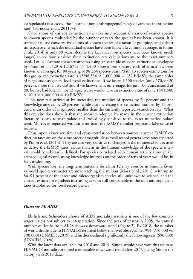
Using the IUCN Red List data, we have shown that approximately 1.5 percent of speciesknown to science have become extinct in the 20 years since IUCN started keeping records.Extinctions are not increasing in an unbounded fashion, however, as seen in Figure 1,where we have included the 2016 and 2020 IUCN data for context.

The cumulative extinction of approximately 1.4 percent of all IUCN characterizedspecies in 2015 is on the order of magnitude of estimates listed by Stork (2010).

8 Social Science Quarterly

Extinction rates reported by Ceballos et al. (2015) confirm the estimates we have pro-vided: A conservative number for mammal extinctions is 1.4 percent of IUCN evaluatedspecies (Ceballos et al., 2015:e1400253) for the time period of 1900–2014, and a con-servative number for other vertebrates is 0.5 percent of IUCN evaluated species (Ceballoset al., 2015:e1400253) for the same time period. Interestingly, Ehrlich, a co-author of theCeballos et al. (2015) study, did not study extinctions over short time spans such as thedecade stipulated in the counterwager (1994–2004). Instead, the Ceballos et al. (2015)authors plotted extinction rates in increments of whole centuries. Clearly, comparing ex-tinction rates over a short time scale and with so little knowledge of actual species numbersis, and was in 1994, a poorly posed problem.

While it appears that Ehrlichs’ (1981) predictions of a 25–50 percent reduction inspecies by 2011 have been exaggerated, others are now raising similar warnings (Barnoskyet al., 2011; Ceballos et al., 2015; Pimm et al., 2014). Current alarm is over group ex-tinction rates compared to background extinction rates. Pimm et al., (2014:1246752-1)explained that “given the uncertainties in species numbers and that only a few percentof species are assessed for their extinction risk, we express extinction rates as fractions ofspecies going extinct over time—extinctions per million species-years (E/MSY) — ratherthan as absolute numbers.” A current extinction rate, once calculated, is then compared toa background extinction rate based on the fossil record (Pimm et al., 2014).

Barnosky et al. (2011:52) defined the concept of the extinction rate as: “[…] essentiallythe number of extinctions divided by the time over which the extinctions occurred.” Back-ground rates of between 0.1 and 2 E/MSY have been reported (Barnosky et al., 2011;Pimm et al., 2014; Ceballos et al., 2015.), yet they were computed over thousands if notmillions of years for species, or more often genera, that had left intelligible fossil traces(Barnosky et al., 2011). Their use as valid background rates for all species has been dis-cussed and challenged even by Barnosky et al. (2011). In fact, Barnosky et al. (2011:52)listed a number of issues concerning extinction rate calculations under the heading “Severedata comparison problems.” These issues included the uneven geographic distribution ofthe fossil record; limited selection of taxa, both fossil and extant, available for compara-tive study; time spans available for comparisons, extending from millions or hundreds ofmillions of years for the fossil record, but not more than 500 years for extant species; andspecies-level versus taxon-level extinction assessments (Barnosky et al., 2011). Barnoskyet al. (2011) have thus hinted at the fact that too often rate comparisons may end up com-paring apples (genera-based rates over very long periods) to oranges (species-based ratesover geologically negligible time periods).

The species versus taxon or genus level assessment is a particularly important problem:“Analyses of fossils are often done at the level of genus rather than species. […] This canresult in lumping species together that are distinct’’ (Barnosky et al., 2011:52). What, thus,would be the comparable genus-level extinction rates from the fossil record? Pimm et al.(2014:1246752-2) have noted that “For mammals, the rate is ∼100 extinctions of generaper million genera years (13) and ∼60 extinctions for birds.” Current extinction rates ofvarious taxonomic groups such as mammals or birds have been reported as varying from107 E/MSY for amphibians to 243 E/MSY for mammals (Barnosky et al., 2011:53; Pimmet al., 2014:1246752-2). Modern species or taxon level extinction rates are thus of the sameorder of magnitude as fossil record genera level extinction rates. Alarm over these highnumbers has prompted article titles such as “Entering the sixth mass extinction” (Ceballoset al., 2015) and “Has the Earth’s sixth mass extinction already arrived?” (Barnosky et al.,2011). However, the extinction rates presented in these articles are the projected currentspecies-level extinction rates based on endangered, not extinct, species numbers. Only such

APPRAISAL OF EHRLICH’S COUNTERBET TO SIMON PART 2 9

extrapolated rates exceed the “’normal (non-anthropogenic) range of variance in extinctionrate” (Barnosky et al., 2011:54).

Calculations of current extinction rates take into account the ratio of extinct speciesto known species multiplied by the number of years the species have been known. It issufficient to use conservative counts of known species of a taxon or grouping, and a shorttimespan over which the individual species have been known (a common average, in Pimmet al., 2014) is only 80 years, despite the fact that most species have been known muchlonger) to see how sensitive these extinction rate calculations are to the exact numbersused. Let us illustrate these sensitivities using an example of avian extinctions developedby Pimm et al., (2014:1246752-1): 1,230 known bird species, each of which has beenknown, on average, for 80 years, give 98,334 species-years. With 13 species extinctions forthis group, the extinction rate is 13/98,334 × 1,000,000 = 132 E/MSY, the same orderof magnitude as genera-level fossil extinctions. If we knew 1,500 species (only 270, or 20percent, more than we do) and if we knew them, on average, for just 100 years instead of80, but we had lost 15, not 13, species, we would have an extinction rate of only 15/(1,500× 100) × 1,000,000 = 10 E/MSY.

This new rate arrived at by increasing the number of species by 20 percent and theknowledge interval by 20 percent, while also increasing the extinction number by 15 per-cent, is an order of magnitude smaller than the currently reported extinction rate. Whatthis exercise does show is that the measure adopted by many in the current extinctionliterature is easy to manipulate and exceedingly sensitive to the exact numerical valuesused. Moreover, reported without error bars, the E/MSY number projects a false sense ofsecurity.

Thus, upon closer scrutiny and cross-correlation between sources, current E/MSY ex-tinction rates are on the same order of magnitude as fossil record genera-level rates reportedby Pimm et al. (2014). They are also very sensitive to changes in the numerical values usedto derive the E/MSY rates, values that, as in the human knowledge of the species inter-val, could be arbitrarily defined. For species correlated with human activity through thearchaeological record, using knowledge intervals on the order of tens of years would be, infact, misleading.

With species loss, the long-term outcome for claim 12 may even be in Simon’s favor,as world species estimates are now reaching 8.7 million (Mora et al., 2011), with up to86–91 percent of the insect and microorganism species still unknown to science, and thecurrent extinction numbers increasing at rates still comparable to the non-anthropogenicrates established for fossil record genera.

Outcome 13: AIDS

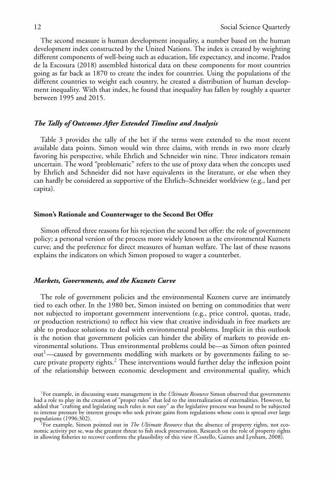
Ehrlich and Schneider’s choice of AIDS mortality statistics is one of the few counter-wager claims not subject to interpretation. Since the peak of deaths in 2005, the annualnumber of deaths from AIDS shows a downward trend (Figure 2). By 2018, the numberof world deaths due to HIV/AIDS returned below the level observed in 1994 (770,000 vs.790,000) (UNAIDS, 2019) and further declined significantly the following year (690,000)(UNAIDS, 2020).

With the latest data available for 2018 and 2019, Simon would have won this claim asHIV/AIDS mortality adopted a noticeable downward trend after 2017, giving Simon thevictory with 2018 data.

10 Social Science Quarterly

FIGURE 2

Deaths from HIV/AIDS, World, 1994–2019

SOURCE: UNAIDS (2019, 2020).

Outcome 14: Sperm Count

As discussed in Part 1 of this two article set, sperm count assessments are difficult toconduct ethically and reliably (Daniels, 2006; Cooper et al., 2010; Levine et al., 2017)and have been subject to selection bias (Deonandan and Jaleel, 2012). Moreover, spermcounts vary by temperature and geography, by ethnic group, and in conjunction withdifferent kinds of physical and mental activity (Daniels, 2006; Swan, Elkin, and Fenster,2000). Possibly the most rigorous early systematic reviews, and subsequent reanalyses, ofmale fertility studies have been conducted by Shanna Swan, Eric Elkin, and Laura Fenster(Swan, Elkin, and Fenster, 1997, 2000). Swan, Elkin, and Fenster (2000) reevaluated 54 ofthe 61 studies presented by Carlsen et al. (1992), then added 47 studies conducted between1934 and 1996, each studying at least ten men using reliable and consistent procedures.Swan, Elkin, and Fenster (2000) offered a comprehensive discussion concluding that from1934 to 1996, sperm counts declined by 1.5 percent in the United States, by 3 percentin both Europe and Australia, but remained unchanged in the so-called “non-Western” or“other” countries (Swan, Elkin, and Fenster, 2000:961, 963). Others concurred, notingthat “[…] the undersampling of rural and less affluent men from low-income countries[,]calls into question researchers’ claims of universally declining semen norms” (Deonandanand Jaleel, 2012:303).

Since 2000, a number of European studies confirmed the decline in sperm density andquality in Western European countries such as France (Burton, 2013; Rolland et al., 2013,on a sample of more than 26,000 men). Swan, Elkin, and Fenster (2000) have noted that

APPRAISAL OF EHRLICH’S COUNTERBET TO SIMON PART 2 11

more studies addressing geographic variation in sperm counts and quality are needed tolearn about the changes in male fertility and their underlying causes.

According to the population by world region data (Roser, Ritchie, and Ortiz-Ospina,2020), in 1994 European and North American populations constituted 17.97 percent ofthe world total; in 2004 their share of global population fell to 16.29 percent. Thus, spermcount declining trends apply to at most, 18 percent of the world while they remain un-known for the majority of world populations (Swan, Elkin, and Fenster, 2000; Deonandanand Jaleel, 2012). As such, the outcome of claim 12 (sperm count) remains uncertain.

It may be worth noting, too, that the decline in sperm density and quality in WesternEuropean countries reported by Burton (2013), among others, is still not catastrophic as“the average estimated sperm count is still well above the level deemed normal by theWorld Health Organization” (Burton, 2013:A46). Swan, Elkin, and Fenster (2000:965)also noted that while much is made of the decline of sperm density and quality as anindicator of environmental decline, more work is needed before these issues are connected.Ongoing research confirms that this claim still cannot be settled globally, merely, withprovisos, for certain well-studied heavily developed geographic areas.

Outcome 15: Inequality

After 2000, estimates of global wealth inequality are far superior to those available pre-2000 even if there are important debates over measurement methodologies. The WorldInequality Lab (part of the WID.world project) is arguably the research group that hasexerted the greatest effort in measuring inequality. The World Inequality Report which theWorld Inequality Lab publishes (Alvaredo et al., 2019) includes nonfinancial assets, unlikethe Oxfam Project, but still falls short of recognizing the full value of the property ownedby the poor, at least if one accepts de Soto’s (2000) estimates. Since 2000, the level ofwealth inequality appears stable, a finding that is confirmed by other sources regardless ofwhether one looks at the top decile or the top centile (Davies, Lluberas, and Shorrocks,2017). Simon thus wins claim 15 as the gap in wealth between the richest 10 percent ofhumanity and the poorest 10 percent is not significantly greater in recent years than it wasin 1994.

However, wealth inequality is a very problematic measure. Generous welfare states en-courage lower savings rates as there are fewer incentives to accumulate wealth for a down-turn (Feldstein, 1974; Kaymak and Poschke, 2016). Age composition of the populationis quite crucial as older populations tend to have more accumulated wealth. Adjusting forage composition of the population leads to dramatically different levels and trends of in-equality (Paglin, 1975; Almås and Mogstad, 2012; Almås, Havnes, and Mogstad, 2011,2012). Inequality trends based on wealth are thus are subject to uncertainty.

What about other measures of inequality? There are two viable substitutes. The first isincome inequality. On that front, there is a clear agreement amongst scholar that globalincome inequality has been falling (Sala-i-Martin, 2006; Liberati, 2015). The measuresdisagree on the extent of the decline, but they all trend downward; see Liberati (2015) fora review of existing measures of inequality. Sala-i-Martin (2006:384) points to changes ininequality between 1979 and 2000 that range between −2.6 and −29.6 percent. There isa key nuance to note here. There is rising inequality within numerous countries, especiallywestern countries. However, there is falling inequality between countries, which dominatesthe effect of inequality within western countries.

12 Social Science Quarterly

The second measure is human development inequality, a number based on the humandevelopment index constructed by the United Nations. The index is created by weightingdifferent components of well-being such as education, life expectancy, and income. Pradosde la Escosura (2018) assembled historical data on these components for most countriesgoing as far back as 1870 to create the index for countries. Using the populations of thedifferent countries to weight each country, he created a distribution of human develop-ment inequality. With that index, he found that inequality has fallen by roughly a quarterbetween 1995 and 2015.

The Tally of Outcomes After Extended Timeline and Analysis

Table 3 provides the tally of the bet if the terms were extended to the most recentavailable data points. Simon would win three claims, with trends in two more clearlyfavoring his perspective, while Ehrlich and Schneider win nine. Three indicators remainuncertain. The word “problematic” refers to the use of proxy data when the concepts usedby Ehrlich and Schneider did not have equivalents in the literature, or else when theycan hardly be considered as supportive of the Ehrlich–Schneider worldview (e.g., land percapita).

Simon’s Rationale and Counterwager to the Second Bet Offer

Simon offered three reasons for his rejection the second bet offer: the role of governmentpolicy; a personal version of the process more widely known as the environmental Kuznetscurve; and the preference for direct measures of human welfare. The last of these reasonsexplains the indicators on which Simon proposed to wager a counterbet.

Markets, Governments, and the Kuznets Curve

The role of government policies and the environmental Kuznets curve are intimatelytied to each other. In the 1980 bet, Simon insisted on betting on commodities that werenot subjected to important government interventions (e.g., price control, quotas, trade,or production restrictions) to reflect his view that creative individuals in free markets areable to produce solutions to deal with environmental problems. Implicit in this outlookis the notion that government policies can hinder the ability of markets to provide en-vironmental solutions. Thus environmental problems could be—as Simon often pointedout1—caused by governments meddling with markets or by governments failing to se-cure private property rights.2 These interventions would further delay the inflexion pointof the relationship between economic development and environmental quality, which

1For example, in discussing waste management in the Ultimate Resource Simon observed that governmentshad a role to play in the creation of “proper rules” that led to the internalization of externalities. However, headded that “crafting and legislating such rules is not easy” as the legislative process was bound to be subjectedto intense pressure by interest groups who seek private gains from regulations whose costs is spread over largepopulations (1996:302).

2For example, Simon pointed out in The Ultimate Resource that the absence of property rights, not eco-nomic activity per se, was the greatest threat to fish stock preservation. Research on the role of property rightsin allowing fisheries to recover confirms the plausibility of this view (Costello, Gaines and Lynham, 2008).

APPRAISAL OF EHRLICH’S COUNTERBET TO SIMON PART 2 13

TAB

LE3

Out

com

eof

the

Ehr

lich–

Sch

neid

er19

95C

ount

erw

ager

Whe

nE

xten

ded

toth

eM

ostR

ecen

tDat

a

Ehr

lich

and

Sch

neid

er’s

Ind

icat

ors

and

Cla

ims,

1994

—M

ostR

ecen

tYea

rfo

rW

hich

Dat

aA

reA

vaila

ble

Can

the

Ind

icat

orB

eM

easu

red

Sat

isfa

ctor

ily?

Win

ner

1.M

ostr

ecen

tyea

rsav

aila

ble

will

onav

erag

eb

ew

arm

erth

an19

92–1

994

Yes

Ehr

lich

and

Sch

neid

er2.

Mor

eca

rbon

dio

xid

ein

atm

osp

here

inm

ostr

ecen

tyea

rav

aila

ble

than

in19

94Ye

sE

hrlic

han

dS

chne

ider

3.M

ore

nitro

usox

ide

inat

mos

phe

rein

mos

trec

enty

ear

avai

lab

leth

anin

1994

Yes

Ehr

lich

and

Sch

neid

er4.

Con

cent

ratio

nof

ozon

e(t

rop

osp

here

)g

reat

erin

mos

trec

enty

ear

avai

lab

leth

an19

94N

og

lob

ald

ata

avai

lab

leU

ncer

tain

(tre

ndfa

vors

Sim

on)

5.E

mis

sion

sof

sulfu

rd

ioxi

de

inA

sia

sig

nific

antly

gre

ater

inm

ostr

ecen

tyea

rav

aila

ble

than

in19

94.

Yes

Ehr

lich

and

Sch

neid

er(t

rend

favo

rsS

imon

)6.

Less

fert

ilecr

opla

ndp

erp

erso

nin

mos

trec

enty

ear

avai

lab

leth

anin

1994

Pro

ble

mat

ic,

(pro

xy:

farm

land

)

Ehr

lich

and

Sch

neid

er

7.Le

ssag

ricul

tura

lsoi

lper

per

son

inm

ostr

ecen

tyea

rav

aila

ble

than

in19

94P

rob

lem

atic

(pro

xy:

farm

land

)

Ehr

lich

and

Sch

neid

er

8.O

nav

erag

ele

ssric

ean

dw

heat

gro

wn

per

per

son

inm

ostr

ecen

tyea

rav

aila

ble

than

in19

92–1

994

Yes/

yes

Sim

on

9.In

dev

elop

ing

natio

nsle

ssfir

ewoo

dav

aila

ble

per

per

son

inm

ostr

ecen

tyea

rav

aila

ble

than

in19

94P

rob

lem

atic

(pro

xy:w

ood

fuel

harv

esta

ndp

rod

uctio

n)

Ehr

lich

and

Sch

neid

er

Con

tinue

d

14 Social Science Quarterly

TAB

LE3

Con

tinue

d

Ehr

lich

and

Sch

neid

er’s

Ind

icat

ors

and

Cla

ims,

1994

—M

ostR

ecen

tYea

rfo

rW

hich

Dat

aA

reA

vaila

ble

Can

the

Ind

icat

orB

eM

easu

red

Sat

isfa

ctor

ily?

Win

ner

10.R

emai

ning

area

ofvi

rgin

trop

ical

moi

stfo

rest

ssi

gni

fican

tlysm

alle

rin

inm

ost

rece

ntye

arav

aila

ble

than

in19

94P

rob

lem

atic

(pro

xies

:hum

idtro

pic

alfo

rest

def

ores

tatio

n)

Ehr

lich

and

Sch

neid

er

11.O

cean

icfis

herie

sha

rves

tper

per

son

will

cont

inue

itsd

ownw

ard

trend

and

thus

inm

ostr

ecen

tyea

rav

aila

ble

will

be

smal

ler

than

in19

94Ye

sE

hrlic

han

dS

chne

ider

12.F

ewer

pla

ntan

dan

imal

spec

ies

still

exta

ntin

mos

trec

enty

ear

avai

lab

leth

anin

1994

Pro

ble

mat

ic(p

roxy

:IU

CN

Red

List

;no

relia

ble

estim

ate

ofg

lob

alsp

ecie

s)

Unc

erta

in

13.M

ore

peo

ple

will

die

ofA

IDS

inm

ostr

ecen

tyea

rav

aila

ble

than

did

in19

94Ye

sS

imon

(afte

r20

18)

14.B

etw

een

1994

and

mos

trec

enty

ear

avai

lab

le,s

per

mco

unts

ofhu

man

mal

esw

illco

ntin

ueto

dec

line

No

glo

bal

dat

aav

aila

ble

Unc

erta

in

15.T

heg

apin

wea

lthb

etw

een

the

riche

st10

per

cent

ofhu

man

ityan

dth

ep

oore

st10

per

cent

will

be

gre

ater

inm

ostr

ecen

tyea

rav

aila

ble

than

in19

94P

rob

lem

atic

(inco

mp

lete

dat

a)

Sim

on

Tally

Sim

on:3

Ehr

lich

and

Sch

neid

er:9

Unc

erta

in:3

APPRAISAL OF EHRLICH’S COUNTERBET TO SIMON PART 2 15

means that indicators could deteriorate for a longer period of time until showing signs ofimprovement.

This viewpoint can be observed in claims 1 and 2 related to climate change. In this case,government subsidies to transport fuels will result in greater greenhouse gas emissions thanwould have otherwise been the case. Numerous studies have thus found that eliminatingthese subsidies would reduce worldwide greenhouse gases (GHG) emissions by somewherebetween 5 and 36 percent (Larsen and Shah, 1992; Burniaux and Chateau, 2014; Inter-national Energy Agency and Organization of Economic Cooperation and Development,2010; Stefanski, 2016). Thus, Simon’s free-market arguments are not disproved by thebet’s outcome.

Similarly, one can identify environmental Kuznets curve patterns with regard to ozone,sulfur dioxide, biodiversity and forest cover. For ozone and sulfur dioxide, the Kuznets-type curves suggest that that the time period of the bet was ahead of the peak point. Thismeans that if current developments continue, the ozone and sulfur dioxide outcomes willeventually favor Simon.

However, it is in the case of biodiversity that the interplay between government policiesand the environmental Kuznets curve is most noticeable. Arrow et al. (1995) and Raymond(2004) pointed out that Kuznets-type relationships are rarer in situations where there areissues of national boundaries and costs spread out over multiple generations. The study ofbiodiversity is subject to such problems and often delivers mixed or contradictory results.Some studies thus fail to identify a statistically significant Environmental Kuznets Curve(EKC) inflexion point (Raymond, 2004; Asafu-Adjaye, 2003), while others do (McPher-son and Nieswiadomy, 2005; Mills and Waite, 2009). What is particularly interestingabout those papers is that their authors make the case that Kuznets-curve relationshipsneed to be examined with a better understanding of the impact of existing institutional ar-rangements. When institutions are included and measured with Simon’s preferred metric(the economic freedom index), the inflexion point is significant and occurs earlier (Panditand Laband, 2009).3 Simon was thus arguably correct to suggest that improvements wouldbe forthcoming conditional on letting markets work and confining government actions tointernalizing externalities.

Forest transition provides another illustration of this interplay between “good” institu-tions and the environmental Kuznets curve. Barbier (2019) thus points out that institu-tional quality, proxied by variables such as the enforcement of property rights, which area key component of economic freedom indexes, can hasten forest recovery. In this, Bar-bier echoes other work suggesting the presence of a Kuznets curve with regard to forestcover (Cuaresma et al., 2017; Benedek and Ferto, 2020; Bhattarai and Hammig, 2001;Murtazashvili, Murtazashvili, and Salahodjaev, 2019). Also in line with Simon’s worldviewis that much evidence suggests that government ownership, mismanagement, and subsi-dies are major drivers of tropical deforestation while strengthening the land and resourcerights of native populations typically results in both better stewardship and lower rates ofdeforestation (Stevens et al., 2014). The combination of these elements suggests that it islikely that, along with a better definition and strengthening of ownership rights, economicdevelopment will in time deliver a forest transition in which greater wealth and populationnumbers are correlated with an expansion of the forest cover in tropical regions.

3Using the IUCN’s percentage of species in each country that were on the Red List of threatened species in2004, Pandit and Laband (2009) found that initial increases in economic freedom led to greater proportions ofspecies being lost. However, there was an early inflexion point, which suggested that, past that threshold, fewerand fewer species were threatened as economic freedom increased. The effect was statistically significant formammals and vascular plants and income also had no statistically significant effects once economic freedomwas controlled for.

16 Social Science Quarterly

Simon’s Counterbet

When he rejected Ehrlich and Schneider’s offer, Simon stated he would rather use “mea-sures of actual welfare, rather than intermediate conditions.” Without formally proposinga new bet, Simon (n.d.) suggested some indicators on which he would be willing to wager:“mortality and morbidity,” “life expectancy,” “future calorie intake, food prices, or foodoutput,” “fish consumption which includes (…) fish farming” and “skin cancer death” (toreflect ozone-related problems).

Shifting to these indicators gives Simon’s a clear win. For example, in Table 2 we alreadyshowed that the overall food supply (measured in calories per capita) has increased over thetime window of the bet, which explains why global indicators of malnutrition have shownmarked improvements in recent decades (Roser and Ritchie, 2013). Life expectancy atbirth rose from 66.1 years in 1994 to 68.7 in 2004 and 72.6 in 2018 (World Bank, 2020).When wild catch and aquaculture fisheries are added to each other, fish consumption percapita increased 7 percent from 1994 to 2004 and a further 17 percent to 2015 (FAO,2020b). Simon would only lose with regard to one of his proposed indicators: skin cancerrates which, when age-standardized, have increased mildly since 1995 (IHME, 2020).4

Reflective Conclusion

Because of the nature of their original bet, the debate between Ehrlich and Simon isoften mistakenly reduced to the nominal price and future availability of natural resourceswhile the true object of the debate was human welfare and its relation to the environment.To Paul Ehrlich, any increase in population numbers and well-being were ultimately un-sustainable because of the finite nature and limited carrying capacity of our environment.His counteroffer reflects this view. To Simon, markets and population growth provide so-lutions to environmental problems conditional on “good” institutions. In a certain way,even though it was never accepted, the second bet offers deeper insights into the complexviews of both Ehrlich and Simon and those who follow in their footsteps.

On its own terms, the second bet is a victory for Ehrlich (and Schneider) in spite of nu-merous uncertainties regarding some indicators. Even when the time horizon is extended,Simon loses to Ehrlich and Schneider. Yet, Ehrlich and Schneider’s claims on topics suchas fertile cropland, agricultural soil, and fuelwood per capita, while correct, can arguablybe interpreted as actual evidence of environmental improvement.

Simon’s key priority and main contribution to the environmental debate was the assem-bling and communication of data. His critique of the proposed second bet, however, alsohighlighted another component of his worldview that was often downplayed or ignoredby his critics, that is, the crucial role that institutions play in determining the relationshipbetween the environment and economic development. As economist Mokyr (2003:60)pointed out: “what seem to be failures of technology are often the failures of institutions.”Simon thus occasionally expressed the view that many real environmental problems werecaused in large part by poorly secured property rights, high barriers to entrepreneurial ac-tivity, and government interventions that distort price signals. As such, they often had littleif anything to do with anthropogenic pressures on a limited stock of resources and fragileecosystems.

4In 1994, the age-standardized death rates for nonmelanoma skin cancer rose from 0.821 per 100,000 to0.826 per 100,000 in 2004 to 0.849 in 2017 (IHME, 2020).

APPRAISAL OF EHRLICH’S COUNTERBET TO SIMON PART 2 17

In the end, we do not doubt that both Simon and Ehrlich shared the same goals of im-proving human standards of living and reducing pressures on ecosystems. Their visions toachieve these outcomes, however, were almost completely opposite. The fact that Ehrlichand Schneider’s own choice of indicators yielded mixed results in the long run, coupledwith the fact that Simon’s preferred indicators of direct human welfare yielded largely fa-vorable outcomes is, in our opinion, sufficient to claim that Simon’s optimistic perspectivewas once again largely validated.

REFERENCES

Aas, Wenche, Augustin Mortier, Van Bowersox, Ribu Cherian, Greg Faluvegi, Hilde Fagerli, Jenny Hand,Zbigniew Klimont, Corinne Galy-Lacaux, Christopher M.B. Lehmann, Cathrine Lund Myhre, GunnarMyhre, Dirk Olivié, Keiichi Sato, Johannes Quaas, P. S.P. Rao, Michael Schulz, Drew Shindell, Ragnhild B.Skeie, Ariel SteinShow lessToshihiko Takemura, Svetlana Tsyro, Robert Vet, and Xiaobin Xu. 2019 “Globaland Regional Trends of Atmospheric Sulfur.” Scientific Reports 9(1):1–11.

Arrow, Kenneth, Bert Bolin, Robert Costanza, Partha Dasgupta, Carl Folke, C. S. Holling, C. S., Bengt-OweJansson, Simon Levin, Karl-Goran Maler, Charles Perrings, and David Pimentel. 1995. “Economic growth,Carrying capacity, and the Environment.” Ecological Economics, 15(2):91–95. https://EconPapers.repec.org/RePEc:eee:ecolec:v:15:y:1995:i:2:p:91-95.

Alexandratos, Nikos, and Jelle Bruinsma. 2012. World Agriculture Towards 2030/2050: The 2012 Revision.Rome: FAO.

Almås, Ingvild, Tarjei Havnes, and Magne Mogstad. 2011. “Baby Booming Inequality? Demographic Changeand Earnings Inequality in Norway, 1967–2000.” Journal of Economic Inequality 9(4):629–50.

———. 2012. “Adjusting for age Effects in Cross-Sectional Distributions.” Stata Journal 12(3):393–405.

Almås, Ingvild, and Magne Mogstad. 2012. “Older or Wealthier? The Impact of Age Adjustment on WealthInequality.” Scandinavian Journal of Economics 114(1):24–54.

Alvaredo, Facundo, Lucas Chancel, Thomas Piketty, Emmanuel Saez, and Gabriel Zucman. 2019. WorldInequality Report, 2018: Executive Summary. Paris: World Inequality Lab.

Asafu-Adjaye, John. 2003. “Biodiversity Loss and Economic Growth: A Cross-Country Analysis.” Contempo-rary Economic Policy 21(2):173–85.

Ausubel, Jesse H. 2015. “The Return of Nature: How Technology Liberates the Environment.” BreakthroughJournal 5(Spring). Available at 〈http://thebreakthrough.org/index.php/journal/issue-5/the-return-of-nature〉.Ausubel, Jesse H., Iddo K. Wernick, and Paul E. Waggoner. 2013. “Peak Farmland and the Prospect of LandSparing.” Population and Development Review 38(S1):221–42.

Bailis, Rob, Yiting Wang, Rudi Drigo, Adrian Ghilardi, and Omar Masera. 2017. Environmental ResearchLetters 12(11):115002. 〈https://doi.org/10.1088/1748-9326/aa83ed〉Baillie, Jonathan E. M., Craig Hilton-Taylor, and Simon N. Stuart. 2004. IUCN Red List of Threat-ened Species: A Global Species Assessment. Cambridge, UK: IUCN Publications Services Unit. Available at〈https://portals.iucn.org/library/sites/library/files/documents/RL-2004-001.pdf〉.Barbier, Edward B. 2019. “Institutional Constraints and the Forest Transition in Tropical Developing Coun-tries.” International Advances in Economic Research 25(1):1–18.

Barnosky, Anthony D., Nicholas Matzke, Susumu Tomiya, Guinevere O. U. Wogan, Brian Swartz, TiagoB. Quental, Charles Marshall, Jenny L. McGuire, Emily L. Lindsey, Kaitlin C. Maguire, Ben Mersey, andElizabeth A. Ferrer. 2011. “Has the Earth’s Sixth Mass Extinction Already Arrived?” Nature 471:51–57.

Bartkowski, Bartosz. 2016. “Are Diverse Ecosystems More Valuable? A Conceptual Framework for EconomicValuation of Biodiversity.” UFZ Discussion Papers, No. 9/2016. Available at 〈http://hdl.handle.net/10419/144178〉.Benedek, Zsófia, and Imre Ferto. 2020. “Does Economic Growth Influence Forestry Trends? An Environmen-tal Kuznets Curve Approach Based on a Composite Forest Recovery Index.” Ecological Indicators 112:106067.

18 Social Science Quarterly

Bhattarai, Madhusudan, and Michael Hammig. 2001. “Institutions and the Environmental Kuznets Curve forDeforestation: A Crosscountry Analysis for Latin America, Africa and Asia.” World Development 29(6):995–1010.

Bruce, Nigel, Rogelio Perez-Padilla, and Rachel Albalak. 2000. “Indoor Air Pollution in Developing Coun-tries: A Major Environmental and Public Health Challenge.” Bulletin of the World Health Organization78(9):1078–92. Available at 〈http://www.who.int/bulletin/archives/78(9)1078.pdf〉.Burniaux, Jean-Marc, and Jean Chateau. 2014. “Greenhouse Gases Mitigation Potential and Economic Effi-ciency of Phasing-Out Fossil Fuel Subsidies.” International Economics 140:71–88.

Burton, Adrian. 2013. “Study Suggests Long-term Decline in French Sperm Quality.” Environmental HealthPerspectives. Available at 〈http://ehp.niehs.nih.gov/121-a46/〉.Carlsen, Elisabeth, Aleksander Giwercman, Niels Keiding, and Niels E. Skakkebæk. 1992. “Evidence forDecreasing Quality of Semen during the Past Fifty Years.” British Medical Journal 305:609–12.

Ceballos, Gerardo, Paul R. Ehrlich, Anthony D. Barnosky, Andres Garcia, Robert M. Pringle, and Todd M.Palmer. 2015. “Accelerated Modern Human-Induced Species Losses: Entering the Sixth Mass Extinction.”Science Advances 1:e1400253. 〈https://doi.org/10.1126/sciadv.1400253〉.Cooper, T. G., E. Noonan, S. von Eckardstein, J. Auger, H. W. Baker, H. M. Behre, T. B. Haugen, T.Kruger, C. Wang, M. T. Mbizvo, and K. M. Vogelsong. 2010. “World Health Organization Reference Valuesfor Human Semen Characteristics.” Human Reproduction Update 16(3):231–45. 〈https://doi.org/10.1093/humupd/dmp048〉.Costello, Christopher, Steven Gaines, and John Lynham. 2008. “Can Catch Shares Prevent Fisheries Col-lapse.” Science 321(5896):1678–81.

Costello, Christopher, and Michael Ward. 2006. “Search, Bioprospecting, and Biodiversity Conservation.”Journal of Environmental Economics and Management 52:615–26.

Craft, Amy B., and R. David Simpson. 2001. “The Value of Biodiversity in Pharmaceutical Research withDifferentiated Products.” Environmental and Resource Economics 18:1–17.

Cuaresma, Jesús Crespo, Olha Danylo, Steffen Fritz, Ian McCallum, Michael Obersteiner, Linda See and BrianWalsh. 2017 “Economic Development and Forest Cover: Evidence from Satellite Data.” Scientific Reports7:40678.

Daniels, Cynthia R. 2006. Exposing Men: The Science and Politics of Male Reproduction. New York: OxfordUniversity Press. 〈https://doi.org/10.1093/acprof:oso/9780195148411.003.0011〉.Davies, James B., Rodrigo Lluberas, and Anthony F. Shorrocks. 2017. “Estimating the Level and Distributionof Global Wealth, 2000–2014.” Review of Income and Wealth 63(4):731–59.

Deaton, Angus. 2013. The Great Escape: Health, Wealth, and the Origins of Inequality. Princeton, NJ: PrincetonUniversity Press.

Deonandan, Raywat, and Marya Jaleel. 2012. “Global Decline in Semen Quality: Ignoring the DevelopingWorld Introduces Selection Bias.” International Journal of General Medicine 5:303–306.

Earth System Research Laboratories (NOAA ESRL). 2020. Trends in Atmospheric Carbon Dioxide. Wash-ington, DC: National Oceanographic and Atmospheric Administration. Available at 〈https://www.esrl.noaa.gov/gmd/ccgg/trends/data.html〉.Ehrlich, Paul R., and Anne H. Ehrlich. 1981. Extinction: The Causes and Consequences of the Disappearance ofSpecies. New York, NY: Random House.

———. 1996. Betrayal of Science and Reason: How Anti-Environmental Rhetoric Threatens Our Future. Wash-ington, DC: Island Press.

Elahi, R., M. I. O’Connor, J. E. Byrnes, J. Dunic, B. K. Eriksson, M. J. Hensel, and P. J. Kearns. 2015. “Re-cent Trends in Local-Scale Marine Biodiversity Reflect Community Structure and Human Impacts.” CurrentBiology 25(14):1938–43.

Environmental Protection Agency (EPA). 2016. Draft Inventory of U.S. Greenhouse Gas Emissions and Sinks:1990–2014. Washington, DC: U.S. Environmental Protection Agency.

Faegri, Knut. 1988. “Preface.” Pp. 1–2 in Hilary H. Birks, H. J. Birks, Peter Emil Kaland, and Dagfinn Moe,eds., The Cultural Landscape. Past Present and Future. Cambridge: Cambridge University Press.

APPRAISAL OF EHRLICH’S COUNTERBET TO SIMON PART 2 19

Feldstein, Martin. 1974. “Social Security, Induced Retirement, and Aggregate Capital Accumulation.” Journalof Political Economy 82(5):905–26.

Federico, Giovanni. 2005. [JS1] Feeding the World: An Economic History of Agriculture, 1800–2000. Princeton:Princeton University Press.

Folberth, Christian, Nikolay Khabarov, Juraj Balkovic, Ratislav Skalsky, Piero Visconti, Philippe Ciais, Ivan A.Janssens, Josep Penuelas, and Michael Obersteiner. 2020. “The Global Cropland-Sparing Potential of High-Yield Farming.” Nature Sustainability 3:281–89.

Food and Agricultural Organization (FAO). 2020a. FAOSTAT. Available at 〈http://www.fao.org/faostat/en/#data/RL〉.———. 2020b. FISHSTAT. Available at 〈http://www.fao.org/faostat/en/#data/RL〉.Food and Agriculture Organization of the United Nations (FAO). 2010. Global Forest Resources Assessment2010: Main Report. Rome: FAO. Available at 〈http://www.fao.org/docrep/013/i1757e/i1757e.pdf〉.———. 2016. The State of World Fisheries and Aquaculture 2016. Contributing to Food Security and Nutritionfor All. Rome: FAO. Available at 〈http://www.fao.org/3/a-i5555e.pdf〉.Gaudel, A., O. R. Cooper, G. Ancellet Barret, B. A. Boynard, J. P. Burrows, C. Clerbaux, P.-F. Coheur, J.Cuesta Cuevas, E. D. Doniki, G. Dufour, F. Ebojie, G. Foret, O. Garcia, M. J. Granados-Muñoz, J. W. Han-nigan, F. Hase, B. Hassler, G. Huang, D. Hurtmans, D. Jaffe Jones, N. P. Kalabokas, B. Kerridge, S. Kulawik,B. Latter, T. Leblanc, E. Le Flochmoën, W. Lin, J. Liu, X. Liu, E. Mahieu, A. McClure-Begley, A. J. L. Neu,M. Osman, M. Palm, H. Petetin, I. Petropavlovskikh, R. Querel, N. A. Rahpoe, A. Rozanov, M. G. Schultz,J. Schwab, R. Siddans, D. Smale, M. Steinbacher, H. Tanimoto, D. Tarasick, V. Thouret, A. M. Thompson,T. Trickl, B. Weatherhead, C. Wespes, H. Worden, C. Vigouroux, X. Xu, G. Zeng, and J. R. Ziemke. 2018.“Tropospheric Ozone Assessment Report: Present-Day Distribution and Trends of Tropospheric Ozone Rele-vant to Climate and Global Atmospheric Chemistry Model Evaluation.” Elementa: Science of the Anthropocene6(1):39.

Gentry, Rebecca R., Halley E. Froehlich, Dietmar Grimm, Peter Kareiva, Michael Parke, Michael Rust, StevenD. Gaines, and Benjamin S. Halpern. 2017. “Mapping the Global Potential for Marine Aquaculture.” NatureEcology & Evolution 1:1317–24.

Goklany, Indur. 2009. “Have Increases in Population, Affluence and Technology Worsened Human andEnvironmental Well-Being?” Electronic Journal of Sustainable Development 1(3):3–28. Available at 〈http://goklany.org/library/EJSD%202009.pdf〉.Golinska, Beata. 2014. “Amazonian Dark Earths in the Context of Pre-Columbian Settlements.” Geology,Geophysics & Environment 40(2):219–32.

Heckenberger, Michael J., J. Christian Russell, Carlos Fausto, Joshua R. Toney, Morgan J. Schmidt, EdithePereira, Bruna Franchetto, and Afukaka Kuikuro. 2008. “Pre-Columbian Urbanism, Anthropogenic Land-scapes, and the Future of the Amazon.” Science 321(5893):1214–7.

Heckenberger, Michael, and Eduardo Góes Neves. 2009. “Amazonian Archaeology.” Annual Review of An-thropology 38:251–66.

Institute for Health Metrics and Evaluation (IHME). 2020. Global Burden of Disease. Available at 〈http://www.healthdata.org/gbd〉.International Energy Agency and Organization for Economic Cooperation and Development. 2010. WorldEnergy Outlook 2010. Paris: International Energy Agency and Organisation for Economic Cooperation andDevelopment.

IUCN. 2016. The IUCN Red List of Threatened Species. Version 2016-2. Available at 〈http://www.iucnredlist.org〉.———. 2020. The IUCN Red List of Threatened Species. Version 2020-2. Available at 〈https://www.iucnredlist.org〉.Kauppi, Pekka E., Jesse H. Ausubel, Jingyun Fang, Alexander S. Mather, Roger A. Sedjo, and Paul E. Wag-goner. 2006. “Returning Forests Analyzed with the Forest Identity.” Proceedings of the National Academy ofSciences 103(46):17574–79.

Kaymak, Barıs, and Markus Poschke. 2016. “The Evolution of Wealth Inequality over Half a Century: TheRole of Taxes, Transfers and Technology.” Journal of Monetary Economics 77:1–25.

20 Social Science Quarterly

Klein Goldewijk, Kees, A. Beusen, G. Van Drecht, and M. De Vos. 2011 “The HYDE 3.1 Spatially Ex-plicit Database of Human-Induced Global Land-Use Change over the Past 12,000 Years.” Global Ecology andBiogeography 20(1):73–86.

Larsen, Bjorn, and Anwar Shah. 1992. World Fossil Fuel Subsidies and Global Carbon Emissions. Washington,DC: World Bank.

Levine, Hagai, Niels Jørgensen, Anderson Martino-Andrade, Jaime Mendiola, Dan Weksler-Derri,Irina Mindlis, Rachel Pinotti, and Shanna H. Swan. 2017. “Temporal Trends in Sperm Count:A systematic Review and Meta-regression Analysis.” Human Reproduction Update. Available at〈https://academic.oup.com/humupd/article/doi/10.1093/humupd/dmx022/4035689/Temporal-trends-in-sperm-count-a-systematic-review〉.Levis, C., et al. 2017 “Persistent Effects of Pre-Columbian Plant Domestication on Amazonian Forest Com-position.” Science 355(6328):925–31.

Liberati, Paolo. 2015. “The World Distribution of Income and Its Inequality, 1970–2009.” Review of Incomeand Wealth 61(2):248–73.

Lombardo, Umberto, José Iriarte, Lautaro Hilbert, Javier Ruiz-Pérez, José M. Capriles, and Heinz Veit. 2020.“Early Holocene Crop Cultivation and Landscape Modification in Amazonia.” Nature. 〈https://doi.org/10.1038/s41586-020-2162-7〉 .

McGrath, Matt. 2020. “Crops Were Cultivated in Regions of the Amazon ‘10,000 Years Ago.’”BBC News April 8. Available at 〈https://www.bbc.com/news/science-environment-52217636?fbclid=IwAR2MSoHo7okbZyQR5kGf_sHU_gsiwE-8WE3QKFxWusWeGMRk6xWo4zAbE5E〉.McPherson, Michael A., and Michael L. Nieswiadomy. 2005. “Environmental Kuznets Curve: ThreatenedSpecies and Spatial Effects.” Ecological Economics 55(3):395–407.

Medhaug, Iselin, Martin B. Stolpe, Erich M. Fischer, and Reto Knutti. 2017. “Reconciling ControversiesAbout the ‘Global Warming Hiatus.’” Nature 545(7652):41–47.

Met Office Hadley Centre. 2020. HadCRUT4. Available at 〈https://www.metoffice.gov.uk/hadobs/hadcrut4/〉.Mills, Julianne H., and Thomas A. Waite. 2009. “Economic Prosperity, Biodiversity Conservation, and theEnvironmental Kuznets Curve.” Ecological Economics 68(7):2087–95.

Mokyr, Joel. 2003. “Thinking About Technology and Institutions.” Macalester International 13(1):8.

Mora, C., D. P. Tittensor, S. Adl, A. G. B. Simpson, and B. Worm. 2011. “How Many Species Are There onEarth and in the Ocean?” PLoS Biology 9(8):e1001127. 〈https://doi.org/10.1371/journal.pbio.1001127〉.Moreno-Mateos, D., E. B. Barbier, P. C. Jones, H. P. Jones, J. Aronson, J. A. López-López, Michelle L. Mc-Crackin, Paula Meli, Daniel Montoya, and J. M. R. Benayas. 2017. “Anthropogenic Ecosystem Disturbanceand the Recovery Debt.” Nature Communications 8(1):1–6.

Murtazashvili, Ilia, Jennifer Murtazashvili, and Raufhon Salahodjaev. 2019. “Trust and Deforestation: ACross-Country Comparison.” Forest Policy and Economics 101:111–19.

National Aeronautics and Space Administration (NOAA GISS). 2020. GISS Surface Temperature AnalysisGISTEMP v4. Available at 〈https://data.giss.nasa.gov/gistemp/〉.National Oceanic and Atmospheric Administration (NOAA CDR). 2020. NOAA Climate Data Record (CDR)of MSU and AMSU-A Mean Layer Temperature, UAH Version 6.0. Available at 〈https://data.nodc.noaa.gov/cgi-bin/iso?id=gov.noaa.ncdc:C00961〉.Paglin, Morton. 1975. “The Measurement and Trend of Inequality: A Basic Revision.” American EconomicReview 65(4):598–609.

Pandit, Ram, and David N. Laband. 2009. “Economic Freedom, Corruption, and Species Imperilment: ACross-Country Analysis.” Society and Natural Resources 22(9):805–23.

Pimm, S. L., C. N. Jenkins, R. Abell, T. M. Brooks, J. L. Gittelman, L. N. Joppa, P. H. Raven, C. M.Roberts, and J. O. Sexton. 2014. The Biodiversity of Species and their Rates of Extinction, Distribution, andProtection. Science 344(6187). 〈https://doi.org/10.1126/science.1246752〉.Prados de la Escosura, Leandro. 2018. “Well-Being Inequality in the Long Run.” CEPR Discussion Paper No.DP12920, Available at SSRN: https://ssrn.com/abstract=3178089

APPRAISAL OF EHRLICH’S COUNTERBET TO SIMON PART 2 21

Primack, R. B., A. J. Miller-Rushing, R. T. Corlett, V. Devictor, D. Johns, R. Loyola, Bea Maas, RobinJ. Pakeman, and L. Pejchar. 2018. “Biodiversity Gains? The Debate on Changes in Local-vs Global-ScaleSpecies Richness.” Biological Conservation 219:A1.

Raymond, Leigh. 2004. “Economic Growth as Environmental Policy? Reconsidering the EnvironmentalKuznets Curve.” Journal of Public Policy 24(3):327–48.

Rolland, M., J. Le Moal, V. Wagener, D. Royère, and J. De Mouzon. 2013. “Decline in Semen Concentrationand Morphology in a Sample of 26,609 Men Close to General Population between 1989 and 2005 in France.”Human Reproduction 28(2):462–70.

Roser, Max, and Hannah Ritchie. 2013. “Hunger and Undernourishment.” OurWorldInData.org. Availableat 〈https://ourworldindata.org/hunger-and-undernourishment〉.Roser, Max, Hannah Ritchie, and Esteban Ortiz-Ospina. 2020. “World Population Growth.” OurWorldIn-Data.org. Available at 〈https://ourworldindata.org/world-population-growth〉.Sala-i-Martin, Xavier. 2006. “The World Distribution of Income: Falling Poverty and… Convergence, Pe-riod.” Quarterly Journal of Economics 121(2):351–97.

Simon, Julian Lincoln. n.d. Betting All Human Welfare Will Improve. Available at 〈http://www.juliansimon.com/writings/Articles/EHRLICH6.txt〉.Simon, Julian L. 1996. The Ultimate Resource 2. Princeton, NJ: Princeton University Press http://www.juliansimon.com/writings/Ultimate_Resource/

Simon, Julian Lincoln, and Aaron Wildavsky. 1995. “Species Loss Revisited.” Pp. 346–61 in Julian L. Simon,ed., The State of Humanity. London: Basil Blackwell.

Simpson, R. David. 1997. “Biodiversity Prospecting: Shopping the Wilds Is Not the Key to Conservation.”.Resources for the Future 126:12–15.

Song, Xiao-Peng, Matthew C. Hansen, Stephen V. Stehman, Peter V. Potapov, Alexandra Tyukavina, Eric F.Vermote, and John R. Townshend. 2018 “Global Land Change from 1982 to 2016.” Nature 560(7720):639–43.

de Soto, Hernando. 2000. The Mystery of Capital: Why Capitalism Triumphs in the West and Fails EverywhereElse. New York: Basic Books.

Stefanski, Radoslaw. 2016. Into the Mire: A Closer Look at Fossil Fuel Subsidies. Calgary: School of Public Policyat the University of Calgary.

Stevens, Caleb, Robert Winterbottom, Katie Reytar, and Jenny Springer. 2014. Securing Rights, CombatingClimate Change. How Strengthening Community Forest Rights Mitigates Climate Change. Washington, DC:World Resources Institute and Rights and Resources Initiative. Available at 〈http://www.wri.org/publication/securing-rights-combating-climate-change〉.Stork, Nigel E. 1993. “How Many Species Are There?” Biodiversity and Conservation 2:215–32.

———. 2010. “Re-Assessing Current Extinction Rates.” Biodiversity and Conservation 19:357–71.

Swan, Shanna, Eric P. Elkin, and Laura Fenster. 1997. “Have Sperm Densities Declined? A Reanalysis ofGlobal Trend Data.” Environmental Health Perspectives 105:128–32.

———. 2000. “The Question of Declining Sperm Density Revisited: An Analysis of 101 Studies Published1934–1996.” Environmental Health Perspectives 108:961–66.

Tans, Pieter, and Ralph Keeling 2016. Trends in Atmospheric Carbon Dioxide—Data. NOAA Global Moni-toring Laboratory. Available at 〈https://www.esrl.noaa.gov/gmd/ccgg/trends/data.html〉.UNAIDS. 2019. UNAIDS Data 2019: State of the Epidemic. Available at 〈https://www.unaids.org/sites/default/files/media_asset/2019-UNAIDS-data_en.pdf〉.———. 2020. Global HIV & AIDS Statistics—2020 Fact Sheet. Available at 〈https://www.unaids.org/en/resources/fact-sheet/text=AIDS/2Drelated/20deaths&text=In/202019/2C/20around/20690/20000,1.6/20million/5D/20people/20in/202010〉.United Nations. World Population Prospects, 2015 Revision. Available at 〈https://esa.un.org/unpd/wpp/〉.

22 Social Science Quarterly

Vellend, M., M. Dornelas, L. Baeten, R. Beauséjour, C. D. Brown, P. De Frenne, Sarah C. Elmendorf,Nicholas J. Gotelli, Faye Moyes, Isla H. Myers-Smith, and Magurran, A. E. 2017. “Estimates of Local Biodi-versity Change over Time Stand Up to Scrutiny.”” Ecology 98(2):583–90.

Williams, Michael. 2008. “A New Look at Global Forest Histories of Land Clearing.” Annual Review ofEnvironment and Resources 33:345–67.

World Bank. 2020. World Development Indicators. Available at 〈https://databank.worldbank.org/source/world-development-indicators〉.World Meteorological Organization. 2014. “World Resources Institute.” CAIT—Country Greenhouse GasEmissions Data. Available at 〈http://cait.wri.org/〉.World Resources Institute. 2003. World Resources 2002–2004: Decisions for the Earth: Balance, Voice and Power.Washington, DC: World Resources Institute. https://files.wri.org/s3fs-public/pdf/wr2002_fullreport.pdf.

Young, Hillary S., Douglas J. McCauley, Mauro Galetti, and Rodolfo Dirzo. 2016. “Patterns, Causes, andConsequences of Anthropocene Defaunation.” Annual Review of Ecology, Evolution, and Systematics 47:333–58.