Embed Size (px)
Citation preview
Calhoun: The NPS Institutional Archive
Reports and Technical Reports All Technical Reports Collection
2002
Capital Investment Planning Aid (CIPA):
an optimization-based decision-support
tool to plan procurement and retirement
of naval platforms
Salmeron, Javier
Monterey, California. Naval Postgraduate School
http://hdl.handle.net/10945/730
NPS-OR-02-006
NAVAL POSTGRADUATE SCHOOL Monterey, California
CAPITAL INVESTMENT PLANNING AID (CIPA)—AN OPTIMIZATION-BASED
DECISION-SUPPORT TOOL TO PLAN PROCUREMENT AND RETIREMENT OF
NAVAL PLATFORMS by
Javier Salmeron Robert F. Dell
Gerald G. Brown Anton Rowe
September 2002
Approved for public release; distribution is unlimited. Prepared for: Chief of Naval Operations Assessment Division (N81) 2000 Navy Pentagon
Washington, DC 20350-2000

NAVAL POSTGRADUATE SCHOOL MONTEREY, CA 93943-5000
RADM David R. Ellison Richard Elster Superintendent Provost This report was prepared for Chief of Naval Operations (N81) and funded by Chief of Naval Operations (N81) and the Office of Naval Research. Reproduction of all or part of this report is authorized. This report was prepared by: JAVIER SALMERON ROBERT F. DELL Research Assistant Professor of Operations Research
Associate Professor of Operations Research
GERALD G. BROWN ANTON ROWE Distinguished Professor of Operations Research
Research Associate of Operations Research
Reviewed by: Released by: R. KEVIN WOOD Associate Chairman for Research Department of Operations Research JAMES N. EAGLE DAVID W. NETZER Chairman Associate Provost and Dean of Research Department of Operations Research

REPORT DOCUMENTATION PAGE
Form approved
OMB No 0704-0188 Public reporting burden for this collection of information is estimated to average 1 hour per response, including the time for reviewing instructions, searching existing data sources, gathering and maintaining the data needed, and completing and reviewing the collection of information. Send comments regarding this burden estimate or any other aspect of this collection of information, including suggestions for reducing this burden, to Washington Headquarters Services, Directorate for information Operations and Reports, 1215 Jefferson Davis Highway, Suite 1204, Arlington, VA 22202-4302, and to the Office of Management and Budget, Paperwork Reduction Project (0704-0188), Washington, DC 20503. 1. AGENCY USE ONLY (Leave blank)
2. REPORT DATE September 2002
3. REPORT TYPE AND DATES COVERED Technical Report
4. TITLE AND SUBTITLE CAPITAL INVESTMENT PLANNING AID (CIPA)—AN OPTIMIZATION-BASED DECISION-SUPPORT TOOL TO PLAN PROCUREMENT AND RETIREMENT OF NAVAL PLATFORMS
5. FUNDING RORJK
6. AUTHOR(S) Javier Salmeron, Robert F. Dell, Gerald G. Brown, and Anton Rowe
7. PERFORMING ORGANIZATION NAME(S) AND ADDRESS(ES) Operations Research Department Naval Postgraduate School Monterey, CA 93943-5219
8. PERFORMING ORGANIZATION REPORT NUMBER NPS-OR-02-006
9. SPONSORING/MONITORING AGENCY NAME(S) AND ADDRESS(ES) Chief of Naval Operations Assessment Division (N81) 2000 Navy Pentagon Washington, DC 20350-2000 Office of Naval Research 800 North Quincy Street Arlington, VA 22217-5660
10. SPONSORING/MONITORING AGENCY REPORT NUMBER
11. SUPPLEMENTARY NOTES 12a. DISTRIBUTION/AVAILABILITY STATEMENT
12b. DISTRIBUTION CODE
13. ABSTRACT (Maximum 200 words.) Capital Investment Planning Aid (CIPA) is an optimization-based decision support system custom-built for the U.S. Navy to formulate complete force structure plans that include ship, submarine, and aircraft procurement and retirement schedules over a 30-year planning horizon. This is an important problem, representing a $1 trillion (2002 dollars) commitment by the Navy. Each candidate plan must respect annual budgets in several funding categories, while following Navy planning guidance such as keeping shipyards efficiently employed, limiting the average and/or maximum age of platforms, and meeting Integrated Warfare Architecture (IWAR) requirements. Without CIPA, such alternatives must be manually assembled—a slow, laborious, demanding task fraught with opportunities for clerical error. CIPA offers a graphical interface to organize planning data, accepts ad hoc manual guidance, optimally completes the missing details of any alternate scenario in a second or two, displays its recommendations and their consequences, and provides scenario cataloging and comparison tools. CIPA reduces to minutes the planning cycle from exigent question to exploratory scenarios to PowerPoint slides displaying results. This document describes the planning environment into which CIPA has been introduced, how CIPA works, and shows how CIPA is used. 14. SUBJECT TERMS Military Capital Planning; Investment Planning; Modeling and Simulation; Optimization; Heuristics.
15. NUMBER OF PAGES
130 16. PRICE CODE
17. SECURITY CLASSIFICATION OF REPORT Unclassified
18. SECURITY CLASSIFICATION OF THIS PAGE Unclassified
19. SECURITY CLASSIFICATION OF ABSTRACT Unclassified
20. LIMITATION OF ABSTRACT UL
CAPITAL INVESTMENT PLANNING AID (CIPA)—AN OPTIMIZATION-BASED DECISION-SUPPORT TOOL TO PLAN PROCUREMENT AND RETIREMENT OF NAVAL
PLATFORMS
by
Javier Salmeron**, Gerald Brown*, Robert Dell*, Anton Rowe** Operations Research Department
Naval Postgraduate School Monterey, CA 93943-5001
Abstract
Capital Investment Planning Aid (CIPA) is an optimization-based
decision support system custom-built for the U.S. Navy to formulate complete force structure plans that include ship, submarine, and aircraft procurement and retirement schedules over a 30-year planning horizon. This is an important problem, representing a $1 trillion (2002 dollars) commitment by the Navy. Each candidate plan must respect annual budgets in several funding categories, while following Navy planning guidance such as keeping shipyards efficiently employed, limiting the average and/or maximum age of platforms, and meeting Integrated Warfare Architecture (IWAR) requirements. Without CIPA, such alternatives must be manually assembled—a slow, laborious, demanding task fraught with opportunities for clerical error. CIPA offers a graphical interface to organize planning data, accepts ad hoc manual guidance, optimally completes the missing details of any alternate scenario in a second or two, displays its recommendations and their consequences, and provides scenario cataloging and comparison tools. CIPA reduces to minutes the planning cycle from exigent question to exploratory scenarios to PowerPoint slides displaying results. This document describes the planning environment into which CIPA has been introduced, how CIPA works, and shows how CIPA is used.
* Supported by Office of Naval Research ** Supported by Chief of Naval Operations, Assessment Division (N81)
i

Table of Contents Executive Summary ............................................................................................................ 7 1. Procurement and Retirement Planning for Navy Ships and Aircraft.......................... 2
1.1. IWAR Assessment and Planning ........................................................................ 3 1.2. EPA/TOA............................................................................................................ 4 1.3. Changing Force Structure Priorities.................................................................... 5
2. CIPA Components ...................................................................................................... 9 3. CIPA Integer Linear Program................................................................................... 17
3.1 Mathematical Model Overview .............................................................................. 11 3.2 CIPA Model ............................................................................................................ 12
4. CIPA Graphical User Interface................................................................................. 24 4.1 GUI Basics .............................................................................................................. 24 4.2 Data Screens............................................................................................................ 26
5. CIPA Solver(s).......................................................................................................... 35 5.1 Solvers..................................................................................................................... 35 5.2 Solver Framework................................................................................................... 35
6. CIPA Heuristic.......................................................................................................... 39 6.1 Initial Solution ........................................................................................................ 39 6.2 Basic Search............................................................................................................ 40 6.3 Deep Search ............................................................................................................ 50 6.4 Heuristic Lower Bound........................................................................................... 54
7. Features of the Exact Algorithm............................................................................... 60 7.1 Lower Bound .......................................................................................................... 60 7.2 Upper Bound........................................................................................................... 60
8. CIPA Results............................................................................................................. 64 8.1 Data Used for Testing CIPA................................................................................... 64 8.2 Output Analysis From the Solver ........................................................................... 65 8.3 Comparison Between Heuristic and Exact Solver .................................................. 70
9. CIPA Project Contributions, Deliverables, and Current Status ................................ 73 9.1 Contributions........................................................................................................... 73 9.2 Deliverables ............................................................................................................ 73 9.3 Other Documents .................................................................................................... 75 9.4 Current Status of the CIPA Project......................................................................... 76
Appendix A: Data Structure.............................................................................................. 77 A.1 Entities ................................................................................................................... 77 A.2 Tables of Data ........................................................................................................ 83 A.3 Data and Result Files ............................................................................................. 91
Appendix B: New Versions of the CIPA Solver ............................................................ 105 B.1. Introduction ......................................................................................................... 105 B.2 Ver_26: Dimension .............................................................................................. 106 B.3 Ver_27: Effectiveness .......................................................................................... 107 B.4 Ver_28: End-Effects............................................................................................. 113
References....................................................................................................................... 120
ii

List of Figures
Figure 1.1: The USS Constitution exhibited innovative naval architecture and the latest armament technology.................................................................................................................3
Figure 1.2: Extended Planning Annex/Total Obligated Authority (EPA/TOA)........................4
Figure 1.3: An artist’s rendition of the Lockheed Martin Joint Strike Fighter (JSF). ...............8
Figure 1.4: An artist’s rendition of the Boeing Unmanned Combat Air Vehicle (UCAV). ......8
Figure 2.1: CIPA scheme.........................................................................................................16
Figure 4.1: CIPA Workbook screen organization....................................................................30
Figure 4.2: Budget summary (graphical view). .......................................................................27
Figure 4.3: Mission summary screen for all requirements (graphical view). ..........................27
Figure 4.4: SSN774 Inventory (data view). Procurement and retirement schedule. ..............28
Figure 4.5: SSN774 Production schedule at Eboat (data view)...............................................34
Figure 4.6: F18AB inventory (data view). Procurement and retirement schedule. ................29
Figure 4.7: Amphibs inventory (graphical view).....................................................................29
Figure 4.8: Labor at Bath shipyard (graphical view)...............................................................30
Figure 4.9: Labor for all shipyards (graphical view). ..............................................................30
Figure 4.10: Penalties...............................................................................................................31
Figure 4.11: Detailed ship inventory report.............................................................................31
Figure 4.12: Detailed air inventory report. ..............................................................................32
Figure 4.13: Ship procurement plan report. .............................................................................32
Figure 4.14: Aircraft procurement plan report.........................................................................33
Figure 4.15: SCN expenditure report.......................................................................................33
Figure 4.16: APN expenditure report.......................................................................................34
Figure 5.1: CIPA Solver Flowchart. ........................................................................................36
Figure 5.2: “Optimize” flowchart for the CIPA Solver. ..........................................................38
iii
Figure 6.1: Influence implication of the CIPA objective function ..........................................47
Figure 6.2: Flowchart of Basic Search.....................................................................................43
Figure 6.3a: Ship-Mission strategy. .........................................................................................50
Figure 6.3b: Air-Mission strategy............................................................................................50
Figure 6.4: Labor strategy........................................................................................................52
Figure 6.5a: Budget-Ship strategy. ..........................................................................................53
Figure 6.5b: Budget-Aircraft strategy......................................................................................53
Figure 6.6a: Ship-Retirement strategy. ....................................................................................55
Figure 6.6b: Air-Retirement strategy.......................................................................................55
Figure 6.7a: Joint Ret.-Proc. (Ship) strategy............................................................................57
Figure 6.7b: Joint Ret.-Proc. (Aircraft) strategy. .....................................................................57
Figure 6.8a: Ship Exchange. ....................................................................................................59
Figure 6.8b: Aircraft Exchange................................................................................................59
Figure 6.8c: Ship-Aircraft Exchange. ......................................................................................59
Figure 6.8d: Ship-Plant Exchange. ..........................................................................................59
Figure 8.1: CIPA.log (initialization)........................................................................................66
Figure 8.2: CIPA.log (lower bound and initial solution). ........................................................66
Figure 8.3: CIPA.log (Heuristic Solver). .................................................................................67
Figure 8.4: CIPA.log (Exact Solver and best solution). ..........................................................68
Figure 8.5: CIPA.log (Results summary). ...............................................................................69
Figure 8.6: CIPA.log (Time report). ........................................................................................70
Figure A.1: Entity-relation diagram.........................................................................................85
iv
List of Tables
Table 1. Baseline case: Ship-Mission areas and associated ships. .........................................64
Table 2. Baseline case: Air-Mission areas and associated aircraft. ........................................65
Table 3. Baseline case: Shipyards and ships produced...........................................................65
Table 4. Test cases run with the CIPA ES and the CIPA HS. ................................................72
Table 9.1. Official versions.....................................................................................................80
Table 9.2. .................................................................................................................................81
Table “General” .......................................................................................................................80
Table “Year” ............................................................................................................................81
Table “Ship”.............................................................................................................................83
Table “Aircraft” .......................................................................................................................83
Table “Plant”............................................................................................................................83
Table “Ship-Mission” ..............................................................................................................83
Table “Air-Mission” ................................................................................................................84
Table “Ship-Year” ...................................................................................................................84
Table “Ship-Plant” ...................................................................................................................84
Table “Ship-Ship-Mission”......................................................................................................85
Table “Aircraft-Year” ..............................................................................................................85
Table “Aircraft-Air-Mission” ..................................................................................................86
Table “Plant-Year”...................................................................................................................86
Table “Ship-Mission-Year” .....................................................................................................87
Table “Air-Mission-Year” .......................................................................................................87
Table “Ship-Plant-Year”..........................................................................................................87
Table “Aircraft-Year-Segment”...............................................................................................88
Table “Ship-Plant-Quantity-Budgeting Year Before” .............................................................88
v
Table “Ship-Plant-Quantity-Budgeting Year After” ...............................................................88
Table “Ship-Plant-Quantity-Construction Year Before” .........................................................89
Table “Ship-Plant-Quantity-Construction Year After” ...........................................................89
Table “Control”........................................................................................................................90
Table. Data I/O........................................................................................................................91
Table. Tables and data files. ...................................................................................................92
Table B.1. Solver versions and their characteristics. ............................................................106
Table “Ship-Ship-Mission”....................................................................................................107
Table “Aircraft-Air-Mission” ................................................................................................108
Table “Ship-Mission-Year” ...................................................................................................108
Table “Air-Mission-Year” .....................................................................................................109
Table “Year” ..........................................................................................................................113
Table “Plant”..........................................................................................................................114
Table “Plant-Year”.................................................................................................................114
vi

Executive Summary The Navy’s procurement and retirement planning is part of a complicated Department
of Defense budget planning process. The U. S. Navy will spend more than $1 trillion (2002 dollars) over the next 30 years to procure ships, submarines, and aircraft to enable it to fulfill its missions.
Today, an attack submarine costs more than $2 billion, an aircraft carrier more than $5 billion, and its air wing $5 billion more. The Navy must balance these large capital expenditures with other procurements and maintain an industrial base capable of satisfying its unique requirements.
Capital Investment Planning Aid (CIPA) is a force structure planning tool that can be used to prescribe ship, submarine, and aircraft procurement and retirement schedules over a 30-year planning horizon. Without CIPA, plans must be manually assembled—a slow, laborious, and demanding task fraught with opportunities for clerical error, and limited to a small range of alternatives. CIPA augments manual planning with optimization, recommending the best (or nearly best) yearly force structure procurement and retirement plan based on industrial and budget constraints, as well as mission inventory and force mix requirements. CIPA is the only Navy decision support system that integrates aircraft and ship procurement decisions with fiscal, industrial, and mission requirements to render the best integrated long-term advice.
The primary components of CIPA are a Graphic User Interface (GUI) and a Solver module. The GUI incorporates user-friendly displays to allow a force-structure analyst to easily create and modify a plan, by accepting ad hoc manual guidance, simplifying the visualization and interpretation of results, and facilitating related tasks such as import or export data and results, and organizing planning data. The CIPA Solver is comprised of a fast, custom heuristic that solves a planning scenario in a few seconds, and an exact method that can provide a solution with a finer quantitative assessment of its quality.
The graphical interface to organize planning data accepts ad hoc manual guidance, optimally completes the missing details of any alternative scenario in a second or two, displays its recommendations and their consequences, and provides scenario cataloging and comparison tools. CIPA reduces to minutes the planning cycle from exigent question to exploratory scenarios to PowerPoint slides displaying results.
This document presents an overview of CIPA. We briefly describe the CIPA planning environment, present an integer-linear program at the heart of CIPA, discuss exact and heuristic techniques we employ to solve CIPA, along with their computational performance, and provide an overview of the graphical user interface.
1

1. Procurement and Retirement Planning for Navy Ships and Aircraft1 The Navy’s procurement and retirement planning is only part of a complicated Department of Defense budget planning process. How did this process get so complex?
American defense budgeting began during the Revolution with proposed requisitions for fielding men and armaments, hand-written by the few well-known general officers who were preparing to personally lead these military operations. These requests were for “what I need.” This requirements-based process persisted with some embellishment until after World War II, when the Hoover Commission required (1948) that budgets be defended in terms of function and activities, rather than just numbers of men and amounts of materiel. The Defense Department and its staffs asked for “what we need to be able to achieve these things, by these specific means.” “In 1959, General Maxwell Taylor suggested a ‘mission-oriented’ budget… Congress subsequently asked that the budget for fiscal 1961 be based on ‘functional categories.’ The idea was to replace intermediate military ‘inputs’ by strategic ‘outputs’ directly describing the policy’s intended effects…” [Martin 1988]. Subsequently, Secretary of Defense Robert McNamara introduced the five-year budget programs and a penchant for detailed decision-support that still characterizes defense budgeting. Now, we start with strategy, express this in terms of mission areas, and then eventually expand these into actual requirements for personnel, materiel, and, in particular, major weapons systems.
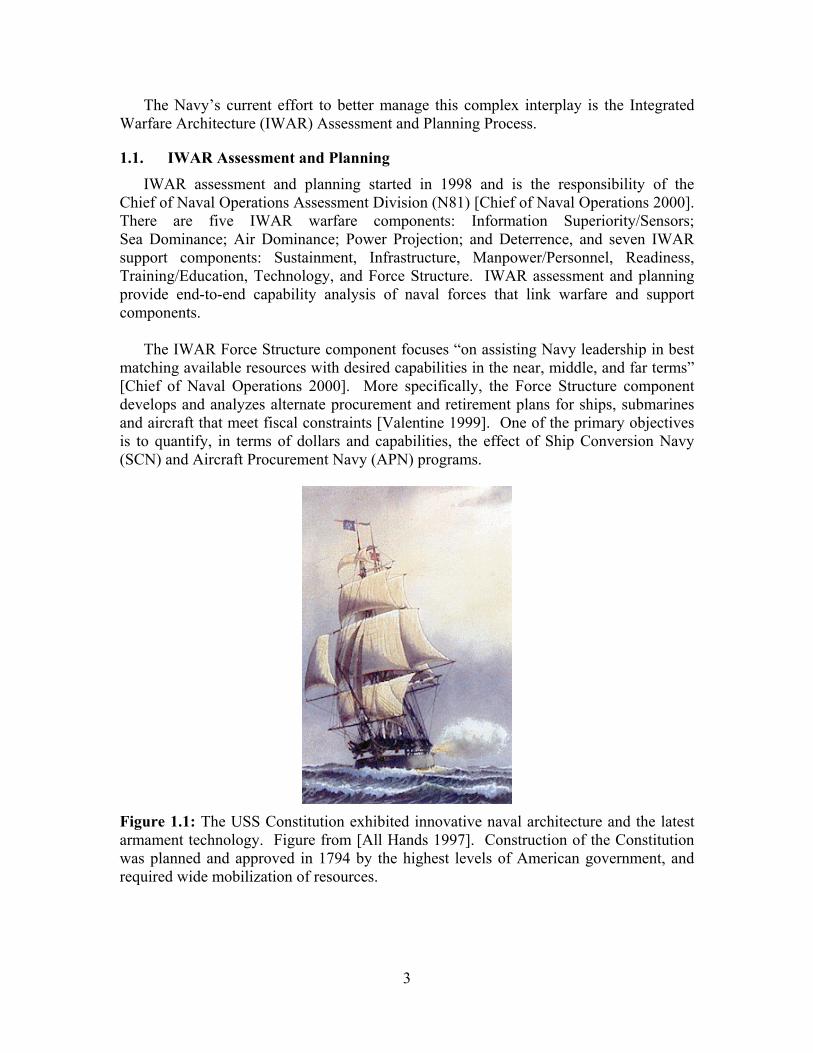
Naval spending has always involved large amounts of resources, research and technology, money, and the attention of civilian and military leadership. In 1794, President Washington asked Congress to authorize construction of six frigates at six different sites to help protect American merchant fleets from attacks by Algerian pirates and harassment by British and French forces [Hagan 1978]. With a total budget exceeding $800,000 (1794 dollars), congressional debate was intense, but construction was ultimately approved on the condition that it be conducted exactly as proposed in six different constituencies, thus affording political insulation. In fiscal year 1999 dollars, the frigates would cost $2.6 billion [Field 1999]. The USS Constitution (shown in Figure 1.1) employed revolutionary technology, used more than 1,500 trees felled from Maine to Georgia, and was armed with cannons cast in Rhode Island [USS CONSTITUTION 1999]. Today, an attack submarine costs more than $2 billion, an aircraft carrier more than $5 billion, and its air wing $5 billion more. These ships are the only current American clients for high-pressure steam nuclear power plants. The Navy must balance these large capital expenditures with other procurements and maintain an industrial base capable of satisfying its unique requirements.
Navy budget analysts must continually respond quickly to scenarios arising from emergent world events and domestic politics. Their advice must consider the complex interplay between past decisions, politics, and fiscal realities.
1 This section relies substantially on text originally found in the first chapter of Field [1999] and the second Chapter of Garcia [2001].
2
The Navy’s current effort to better manage this complex interplay is the Integrated Warfare Architecture (IWAR) Assessment and Planning Process.
1.1. IWAR Assessment and Planning IWAR assessment and planning started in 1998 and is the responsibility of the Chief of Naval Operations Assessment Division (N81) [Chief of Naval Operations 2000]. There are five IWAR warfare components: Information Superiority/Sensors; Sea Dominance; Air Dominance; Power Projection; and Deterrence, and seven IWAR support components: Sustainment, Infrastructure, Manpower/Personnel, Readiness, Training/Education, Technology, and Force Structure. IWAR assessment and planning provide end-to-end capability analysis of naval forces that link warfare and support components. The IWAR Force Structure component focuses “on assisting Navy leadership in best matching available resources with desired capabilities in the near, middle, and far terms” [Chief of Naval Operations 2000]. More specifically, the Force Structure component develops and analyzes alternate procurement and retirement plans for ships, submarines and aircraft that meet fiscal constraints [Valentine 1999]. One of the primary objectives is to quantify, in terms of dollars and capabilities, the effect of Ship Conversion Navy (SCN) and Aircraft Procurement Navy (APN) programs.
Figure 1.1: The USS Constitution exhibited innovative naval architecture and the latest armament technology. Figure from [All Hands 1997]. Construction of the Constitution was planned and approved in 1794 by the highest levels of American government, and required wide mobilization of resources.
3

1.2. EPA/TOA Extended Planning Annex/Total Obligated Authority (EPA/TOA) is the primary tool used by N81 to evaluate specific alternate force structures. Based on input from the warfare IWAR components, resource sponsors, and numerous documented requirements such as the Quadrennial Defense Review (QDR), Defense Planning Guidance (DPG), and Commander in Chief operational plans, analysts perform manual “what-if” scenarios using EPA/TOA. Analysts then compare scenario results to determine the structure that most closely matches projected budgets and meets force size and capability requirements. Systems Planning and Analysis, Incorporated maintains EPA/TOA for N81. EPA/TOA consists of 62 spreadsheets (Figure 1.2) that calculate yearly Military Personnel (MILPERS), Civilian Personnel (CIVPERS), Military Pay Navy (MPN), Operation and Maintenance (O&M), Other Procurement Navy (OPN), Ship Conversion Navy (SCN), Aircraft Procurement Navy (APN), Procurement of Ammunition Navy/Marine Corps (PANMC), Weapon Procurement Navy (WPN), Research Development Technology & Experimentation (RDT&E), Military Construction (MILCON), Family Housing Navy (FHN), National Defense Sea-lift Fund (NDSF), and OTHER monies for input procurements and retirements.
F-14INV
F/A-18INV
E-2INV
P-3INV
JSFINV
SH-60INV
etc.
DONAircraft
InventoryModel
AmphibsMCM
Command
Logistics
EPATOA
Model
25 YEARTOA Estimate
By APPNPlus MILPERS/
CIVPERS
Ship/Aircraft
Inventory(TAI, PAA)
Ship/AircraftAverage
Age
APNPlan
SCNPlan
Support ShipGENCAP
WPNPlan
ShipInventory
Model
AircraftCarriers
SurfaceCombatants
ShipWeight/
GeneratorCapacityDatabase
Figure 1.2: Extended Planning Annex/Total Obligated Authority (EPA/TOA) [Systems Planning and Analysis 1998]. EPA/TOA consists of 62 spreadsheets that are linked to estimate Total Obligated Authority.
4
The current Resource Allocation Display (RAD) in EPA/TOA—a snapshot of the Fiscal Year’s Defense Plan (FYDP) at a specific point in time—is the basis for near-term cost, procurement, and retirement of weapon systems. EPA/TOA fixes TOA in the near term based on the FYDP. For the middle term and far term the analyst manually provides procurements and retirements of weapon systems. EPA/TOA calculates TOA based on cost estimation relationships for the categories of MILPERS, CIVPERS, MPN, O&M, OPN, SCN, APN, PANMC, and WPN monies. The model uses cost analogies—the multiplication of a historic data point by a scalar—to estimate cost for RDT&E, MILCON, FHN, NDSF, and OTHER monies.
Force structure analysts are primarily concerned with the procurement and retirement of ships, submarines, and aircraft. Ships are procured with SCN money and aircraft with APN money. Within EPA/TOA, procurement of ships and aircraft directly affect SCN and APN, and indirectly affect some of the other TOA monies through their respective cost estimation relationships.
Using EPA/TOA is labor intensive and error-prone. For instance, to change the procurement plan for the DDG51 class ship requires an analyst to make synchronous changes to three different spreadsheets, and this is just one of 100 platforms over a 25-year horizon. Each alternative accounts for numerous platform retirements and, recently, the 14 major procurement programs in process or under consideration.
1.3. Changing Force Structure Priorities
N81 planners face many problems determining and dealing with force structure priorities. Priorities change for many reasons including: a new President and administration, world events, and new technologies and systems. CIPA can help address some of the competing priorities and allow planners to quickly explore optimized alternatives in their ever-changing environment. Below we provide some recent examples of scenarios that typify those that must be considered by N81 Force Structure Planners.
The DPG outlines the missions the U.S. military must fulfill to satisfy U.S. National Military Strategy. The George W. Bush administration’s plan for sizing the force structure started with a pledge to put strategic priorities first and budget priorities second [Scarborough 2001a]. President Bush directed Defense Secretary Rumsfeld to conduct a total review of the 1.36 million-person armed forces and reorganize it to meet the 21st century’s threats. President Bush told our troops, “We must put strategy first, then spending. Our defense vision will drive our defense budget; not the other way around.” [Scarborough 2001a]. Secretary Rumsfeld requested a $329 billion budget for 2002, which was the largest one-year defense increase since the 1980s. He implied that the 2002 budget is still considered to have far less funding than required to meet existing National Military Strategy. Secretary Rumsfeld also argued that the armed forces have been so under-funded and overused in the 1990s that one budget cycle cannot repair all the damage [Scarborough 2001a].
Secreatry Rumsfeld stated that the average age of aircraft has gone up about 10 years since the 1990s, and high maintenance costs are consuming the budget [Thomas 2001].
5
The Navy is forced to invest valuable maintenance man-hours on aircraft cannibalization, transferring scarce parts from aircraft to aircraft. He also stated that the “ship-building budget at the current rate is on a trajectory from 310 ships to 230 ships” [Thomas 2001]. The Bush administration’s challenge is persuading Congress to supply the money necessary to rejuvenate the aging fleet.
The initial 2001 QDR stated that U.S. forces must be sized and shaped to perform three major tasks concurrently: defend the U. S. against attacks on the homeland or on defense-related information infrastructure; deter forward in critical areas of the world; and win decisively against an adversary in any one of these critical areas of the world [Grossman 2001]. Secretary Rumsfeld later revised the QDR to eliminate the requirement to perform the major tasks concurrently. This change to QDR guidance reflects the compromises being made to fulfill mission requirements while meeting tight budget realities. Defense planners acknowledge that the mismatch between strategy and resources has created a large number of budget shortfalls. One of these is military modernization. The military wants to get away from having aircraft, ships, and other equipment that are extremely old and drive up operating and maintenance costs [Weinberger 2001].
World events impact our Defense budget and force structure planning. The USS Cole attack [Navy Public Affairs Library, 2000] and the EP-3 collision with a Chinese fighter [Navy Public Affairs Library, 2001] are recent examples with minimal initial impact on naval inventories, but with potential widespread influence on force structure planning.
On 11 September 2001, terrorists crashed two hijacked commercial airliners into the twin towers of the World Trade Center in New York City and a third jet into the Pentagon [Rhem 2001]. In the wake of these terrorist attacks, Congress approved $40 billion in emergency defense funds. The Pentagon plans to spend half of the first $2.5 billion installment on intelligence upgrades and is expected to spend an additional $1 billion with the next installment [Capaccio 2001]. The Pentagon plan is to improve intelligence surveillance and reconnaissance aircraft, to buy more unmanned reconnaissance planes and private-source satellite imagery, and to upgrade the Pentagon's aging fleets of surveillance and tanker aircraft. The Navy is also considering accelerating purchases of C-40 transport planes to replace its much older C-9 cargo planes [Pasztor et al. 2001].
Since President Bush declared war on terrorism, more money has been promised to the Defense Department. The QDR retains 12 Navy carriers [Scarborough 2001b]. The big question is whether more money will be available to upgrade the rest of the fleet. Anti-terrorist operations will place more wear and tear on a combat fleet that already needs updated platforms. Another question is what additional money will be provided to pay for operating and maintaining the Navy’s ships and planes already deployed in support of the war on terrorism.
New technologies and systems change the way we perceive and react to threats. These altered perceptions serve to shape our National Military Strategy, the Defense Planning Guidance, and consequently, our force structure planning. The tri-service,
6

multi-national Joint Strike Fighter (JSF) program (Figure 1.3), V-22 Osprey, Unmanned Combat Air Vehicle (UCAV), and Unmanned Air Vehicle (UAV), are examples of aircraft that will impact our force structure for the next decade and beyond.
The Marine Corps will get $592.3 million less than requested and build nine (instead of 12) V-22 Osprey tilt-rotor aircraft next year under the new defense bill approved by the Senate Armed Services Committee [Whittle 2001]. A special Pentagon panel recommended that Osprey production be held to a minimum while flaws that led to one of last year's crashes are fixed. The Marine Corps wants 360 V-22s to replace Vietnam-era helicopters.
New systems such as the Predator UAV are being used to support intelligence, surveillance, and reconnaissance missions while minimizing risk to our pilots and aircrew. The UCAV in Figure 1.4 is the next step toward minimizing combat fatalities while supporting two major combat roles: Suppression of Enemy Air Defenses (SEAD) and precision strike. The initial operational capability of UCAV is now planned for approximately 2010 [Baker 2001].
The multi-billion dollar JSF, V-22, UAV, and UCAV programs may affect our defense budget for decades, and significantly alter the way we prepare for and fight future battles. Force structure planners require flexible tools to deal with new system capabilities, uncertainties, and vulnerabilities.
7
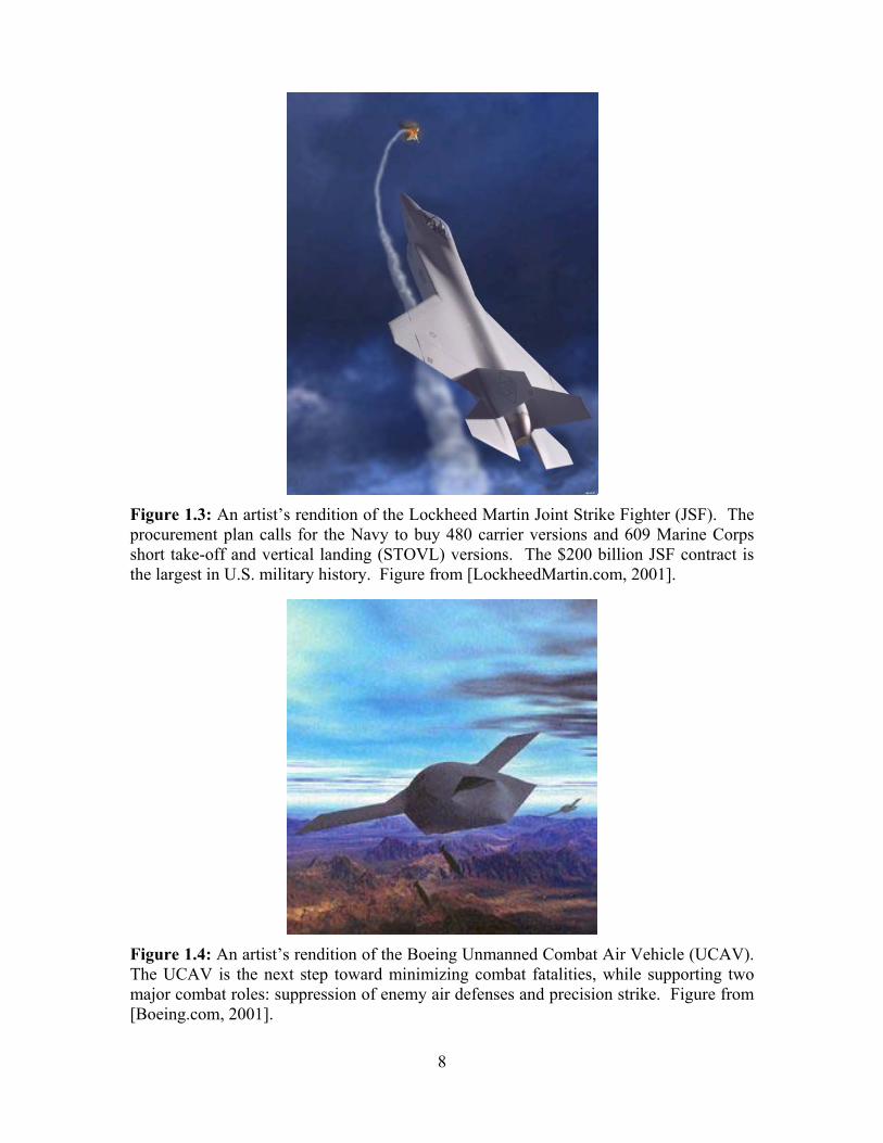
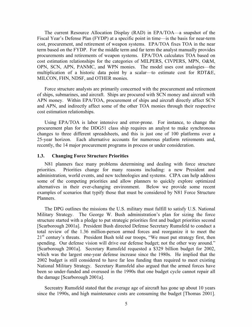
Figure 1.3: An artist’s rendition of the Lockheed Martin Joint Strike Fighter (JSF). The procurement plan calls for the Navy to buy 480 carrier versions and 609 Marine Corps short take-off and vertical landing (STOVL) versions. The $200 billion JSF contract is the largest in U.S. military history. Figure from [LockheedMartin.com, 2001].
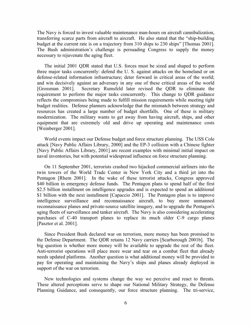
Figure 1.4: An artist’s rendition of the Boeing Unmanned Combat Air Vehicle (UCAV). The UCAV is the next step toward minimizing combat fatalities, while supporting two major combat roles: suppression of enemy air defenses and precision strike. Figure from [Boeing.com, 2001].
8
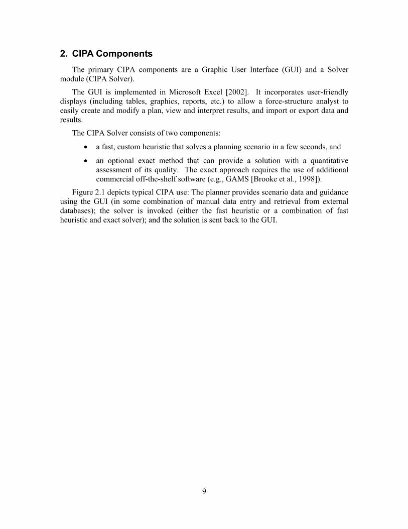
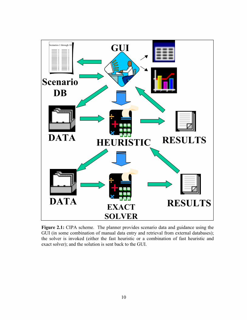
2. CIPA Components The primary CIPA components are a Graphic User Interface (GUI) and a Solver
module (CIPA Solver).
The GUI is implemented in Microsoft Excel [2002]. It incorporates user-friendly displays (including tables, graphics, reports, etc.) to allow a force-structure analyst to easily create and modify a plan, view and interpret results, and import or export data and results.
The CIPA Solver consists of two components:
• a fast, custom heuristic that solves a planning scenario in a few seconds, and
• an optional exact method that can provide a solution with a quantitative assessment of its quality. The exact approach requires the use of additional commercial off-the-shelf software (e.g., GAMS [Brooke et al., 1998]).
Figure 2.1 depicts typical CIPA use: The planner provides scenario data and guidance using the GUI (in some combination of manual data entry and retrieval from external databases); the solver is invoked (either the fast heuristic or a combination of fast heuristic and exact solver); and the solution is sent back to the GUI.
9
10
GUI
DATA
HEURISTIC
EXACT SOLVER
RESULTS
RESULTS DATA
Scenario DB
Scenarios 1 through 10
Figure 2.1: CIPA scheme. The planner provides scenario data and guidance using theGUI (in some combination of manual data entry and retrieval from external databases);the solver is invoked (either the fast heuristic or a combination of fast heuristic and exact solver); and the solution is sent back to the GUI.
3. CIPA Integer Linear Program
3.1 Mathematical Model Overview
CIPA expresses each planning scenario as an integer-linear program minimizing penalties associated with violating budget constraints, production constraints, and inventory requirements. For a recommended plan, CIPA illuminates the required budget, purchase dates and quantities, production facility employment levels, and force levels. CIPA also isolates force level deficiencies inflicted by budget restrictions on procurements, production that cannot keep pace with procurement requirements, or for lack of any existing replacement for retired platforms. CIPA maintains yearly time fidelity for 25 or 30 years. Because it can take up to five years to build platforms, CIPA’s prescriptions for the last few years of the planning horizon may suffer from end effects: The solution for the last years of the horizon may lack accuracy because no information for years beyond the horizon has been specified.
In short, the mathematical model represents the a number of features divided into six categories:
1. Mission: - Ship-mission and air-mission requirements
2. Inventory:
- Initial inventory of ships and aircraft - Ongoing (resident) production of ships and aircraft - Minimum and maximum annual production of ships and aircraft - Maximum total production of ships and aircraft - Maximum annual inventory of ships and aircraft - Minimum and maximum annual ship and aircraft retirement
3. Cost: - Ship and aircraft cost profile - Economy-of-scale for ship and aircraft procurement - Operation and maintenance costs for each ship and aircraft
4. Budget: - Minimum and maximum annual budget available - Minimum and maximum cumulative budget available
5. Industry:
- Work-force profile for ship production - Minimum and maximum annual work-force levels for ship industry
6. Penalty:
- Tradeoff among budget shortfall (or surplus), industry work-force shortfall (or surplus) and mission shortfall
11
Mission requirements (category 1) drive platform procurement. Category 2 features account for yearly platform inventory levels. These impose shipyard capacity, minimum retirement levels, the age of existing platforms, etc. Category 3 considers CIPA cost-related features. Procurement costs are typically incurred and spread out over a number of years before a platform is delivered. The cost of purchasing platforms exhibits economy of scale. Category 4 specifies annual and cumulative expenditures, and should not exceed or fall below their respective specified limits. Category 5 refers to work-force requirements for ship production that are spread out over the production period of a ship. Ideally, workforce levels should stay within specified limits to prevent loss of industrial capability and to avoid overtime costs. The last category refers to CIPA penalty charges for each individual violation of budget, industry, or mission-required levels. The penalties express the tradeoff among the different shortfalls and surpluses in order to prioritize the satisfaction of those conditions deemed more critical by the user.
As main decision variables, we consider the number of platforms procured and retired every year. We add additional variables to specify the piece-wise linear approximation of non-convex cost associated with economies-of-scale. We also incorporate “elastic” variables to account for budget, industry, and mission requirement violations. The objective function expresses the sum of these violations. See Field [1999] for a discussion of how to select penalty values.
All these features are mathematically represented through the following linear program:
CIPA: mins.t. (3.1) to (3.46)
F
where the objective function, F, and the constraints (3.1) and (3.46), are described in detail in the following section.
3.2 CIPA Model This section presents the mathematical formulation of the CIPA model.
3.2.1 Sets and Indices
Time Y, set of years of the planning horizon; Yyy ∈', . For convenience it is assumed that
. {1, 2,3,..., | |}Y Y= Platform
A, set of aircraft types; Aa ∈S, set of ship classes; s S∈
12
Mission
AM , set of air missions; AMm ∈SM , set of Ship-Missions; m SM∈
AAm ⊆ , subset of aircraft types that perform mission AMm ∈
SSm ⊆ , subset of ship classes that perform mission SMm ∈ Production
aI , set of cost increments for aircraft Aa ∈ ; i aI∈
P, set of production facilities; Pp ∈ PPs ⊆ , subset of facilities that produce ship class Ss ∈
spyQ , set of quantities available for ship Ss ∈ procurement at facility in year
. This set is defined in terms of the sPp ∈
Yy ∈spy
sproc and spysproc parameters
(see below) as follows: }1{ spyspyspy sproc,,sproc,Qq +=∈spy
sproc .
Others
+Z , set of non-negative integers, Z }210{ ,...,,=+
3.2.2 Parameters (and Units)
Conventions The word “procurement” or “to procure” refers to “delivery” or “to deliver,” respectively, unless explicitly stated otherwise. Therefore, we refer to “procure” as the action that takes place at the moment (year) that the platform is delivered and available for use from that year onwards, regardless of when the real “procurement” arrangements were made. The words “time period” and “year” will be used interchangeably. The words “shipyard,” “facility,” and “plant” will be used interchangeably. Objective-related parameters: Penalties
ampenm, penalty for shortage in completing Air-Mission ($ per aircraft) AMm ∈smpenm, penalty for shortage in completing Ship-Mission ($ per ship) SMm ∈
+ybpen , penalty for budget excess ($ per $) −ybpen , penalty for budget shortage ($ per $)
+ycbpen , penalty for cumulative expenses excess ($ per $) −ycbpen , penalty for cumulative expenses shortage ($ per $)
13
+plpen , penalty for labor excess at plant Pp ∈ ($ per worker) −plpen , penalty for labor shortage at plant Pp ∈ ($ per worker)
Constraint-related parameters: Used for index dependencies
,SBbsp number of years before (starting at 0) the procurement of ship class Ss ∈
from plant requires budget (i.e., in 0,1,... sPp ∈ 1−spSBb years before) ,SCbsp number of years before (starting at 0) the procurement of ship class Ss ∈
from plant requires labor (i.e., in 0,1,... sPp ∈ 1−spSCb years before)
, number of years after (starting at 1) the procurement of ship class from plant requires budget (i.e., in 0,1,... years before)
SBasp Ss ∈
sPp ∈ spSBa,SCasp number of years after (starting at 1) the procurement of ship class
from plant requires labor (i.e., in 0,1,... years before) Ss ∈
sPp ∈ spSCa,ABba number of years before the procurement of aircraft type a in which
the aircraft is paid (at once) A∈
Constraint-related parameters: Ships
,vsin s
0 initial inventory of class Ss ∈ ships (# ships) ,sycsproc committed procurement of class Ss ∈ ships in year Yy∈ due to
production in progress (# ships) ,vsin s maximum number of class Ss ∈ ships in inventory (# ships) ,spstot maximum number of class Ss ∈ ships to procure from plant
(# ships) sPp ∈
,spy
sproc minimum number of class Ss ∈ ships to procure from plant in
time period (# ships) sPp ∈
Yy∈ Note: ,
spysproc 0= 1-}max{ spsps SCb,SBby;Pp,Ss ≤∀∈∈∀ and
,sprocspy
0= }max{1 spsps SCa,SBa|Y|y;Pp,Ss −+≥∀∈∈∀ is required
,spysproc maximum number of class Ss ∈ ships to procure from plant in time period (# ships)
sPp ∈Yy∈
Note: ,spysproc 0= 1-}max{ spsps SCb,SBby;Pp,Ss ≤∀∈∈∀ and
,sprocspy 0= }max{1 spsps SCa,SBa|Y|y;Pp,Ss −+≥∀∈∈∀ is required.
14
Constraint-related parameters: Aircraft
,ainva0 initial inventory of type Aa ∈ aircraft (# aircraft)
,aycaproc committed procurement of type Aa ∈ aircraft in year due to production in progress (# aircraft)
Yy∈
,ainva maximum number of type Aa ∈ aircraft in inventory (# aircraft) ,aatot maximum number of type Aa ∈ aircraft to procure (# aircraft)
,ay
aproc minimum number of type a A∈ aircraft to procure in time period
(# ships)
Yy∈
,ayaproc maximum number of type Aa ∈ aircraft to procure in time period Yy∈ (# ships)
,ayiinc increment aIi ∈ lower bound for the number of type Aa ∈ aircraft to be procured in year Yy∈ (# aircraft)
,ayiinc increment aIi ∈ upper bound for the number of type Aa ∈ aircraft to be procured in year Yy∈ (# aircraft)
,asquad squadron size for aircraft Aa ∈ procurement (# aircraft) Constraint-related parameters: Retirements
,csret sy minimum cumulative number of class Ss ∈ ships to retire by the end of
time period (# ships) Yy∈
,csret sy maximum cumulative number of class s S∈ ships to retire by the end of time period (# ships) Yy∈
,sret sy minimum number of class Ss ∈ ships to retire by the end of time period (# ships) Yy∈
,sret sy maximum number of class Ss ∈ ships to retire by the end of time period (# ships) Yy∈
,caret ay minimum cumulative number of type Aa ∈ aircraft to retire by the end of time period (# aircraft) Yy∈
,caret ay maximum cumulative number of type Aa ∈ aircraft to retire by the end of time period (# aircraft) Yy∈
,aret sy minimum number of type a A∈ aircraft to retire by the end of time period
(# aircraft) Yy∈
,aret sy maximum number of type Aa ∈ aircraft to retire by the end of time period (# aircraft) Yy∈
15

Constraint-related parameters: Mission inventory
,my
smreq number of ships required for Ship-Mission m in time period SM∈ Yy∈
(# ships) ,
myamreq number of aircraft required for air mission in time period AMm ∈ Yy∈
(# aircraft) Constraint-related parameters: Budget
,yoscn fixed SCN cost in year Yy∈ ($)
,yocscn fixed SCN cost in year Yy∈ for ships not considered ($) ,frac historical fraction of total SCN cost for ship outfitting
,yoapn fixed APN cost in year Yy∈ ($) ,yocapn fixed APN cost in year Yy∈ for aircraft not considered ($)
,5apn historical fraction of total APN categories 1 through 4 required for categories 5 through 7
,oomy fixed O&M cost in year Yy∈ for maintenance not considered ($) ,spqlscostb SCN cost incurred l years before q class-s ships are procured from plant p,
for s , , , S∈ sPp ∈ ∪Yy
spyQq∈
∈ 1}-10{ spSBb,,,l = ($)
,spqlscosta SCN cost incurred l years after q class-s ships are procured from plant p,
for s , , , S∈ sPp ∈ ∪Yy
spyQq∈
∈ }1{ spSBa,,l = ($)
,ayiaacost increment Ii ∈ procurement cost for type a Aa ∈ aircraft in year ($ per aircraft)
Yy∈
,ayiabcost increment Ii ∈ fixed procurement cost (intercept) for type aircraft in year ($)
a
YAa ∈
y∈,omshipsy O&M cost for class Ss ∈ ship in year Yy∈ ($ per ship)
,omairay O&M cost for type Aa ∈ aircraft in year Yy∈ ($ per ship) ,csbudget y committed budget in year Yy∈ due to ship production in progress ($)
,toa y TOA budget lower limit for year Yy∈ ($)
,toa y TOA budget upper limit for year Yy∈ ($) ,ctoa y TOA cumulative budget lower limit for year Yy∈ ($)
,ctoa y TOA cumulative budget upper limit for year Yy∈ ($)
16

Constraint-related parameters: Labor
,claborpy committed labor in year Yy∈ at plant Pp ∈ due to production in progress (# workers)
,sworkbspqn required labor n years before q class-s ships are procured from plant p, for
, , , Ss ∈ sPp ∈ ∪Yy
spyQq∈
∈ 1}-10{ spSCb,,,n = (# workers)
,sworkaspqn required labor n years after q class-s ships are procured from plant p, for
, , , Ss ∈ sPp ∈ ∪Yy
spyQq∈
∈ }1{ spSCa,,n = (# workers)
,pcappy
minimum production capacity at plant Pp ∈ in time period
(# workers)
Yy∈
,pcap py maximum production capacity at plant Pp ∈ in time period (# workers)
Yy∈
3.2.3 Decision Variables (and Units)
Variables related to objective function and to elastic constraints
,F objective function value AMmyα , Air-Mission AMm ∈ shortage in year Yy ∈ (# aircraft) SMmyα , Ship-Mission SMm ∈ shortage in year Yy ∈ (# ships)
+αBy , budget excess in year Yy ∈ ($)
−αBy , budget shortage in year Yy ∈ ($)
+αCBy , cumulative budget excess in year Yy ∈ ($)
−αCBy , cumulative budget shortage in year Yy ∈ ($)
+αLy , labor excess in year Yy ∈ (# workers)
−αLy , labor shortage in year Yy ∈ (# workers)
Main decision variables
,APROCayi number of type Aa ∈ aircraft to procure at the start of year in cost
increment i (# aircraft) Yy∈
aI∈,ARETay number of type Aa ∈ aircraft to retire by the end of year (# aircraft) Yy∈
,SPROCspyq one if facility is to deliver Pp ∈ spyQq ∈ class Ss ∈ ships at the start of year , and zero otherwise (0-1 variable) Yy∈
,SRETsy number of class Ss ∈ ships to retire by the end of year (# ships) Yy∈
17
Control decision variables
,APayi one if aircraft is procured at the start of year Aa ∈ Yy∈ in cost increment i , and zero otherwise (0-1 variable) aI∈
,AINVay inventory of type Aa ∈ aircraft at the start of year Yy∈ (# aircraft)
,AMINVmy inventory for air mission m at the start of year AM∈ Yy∈ (# aircraft) ,SINVsy inventory of class Ss ∈ ships at the start of year Yy∈ (# ships)
,SMINVmy inventory for Ship-Mission at the start of year (# ships) SMm ∈ Yy∈
,SBUDGETy amount of SCN money to budget for year Yy∈ ($) ,ABUDGETy amount of APN money to budget for year Yy∈ ($)
,OMBUDGETy amount of O&M money to budget for year Yy∈ ($) , total amount of money to budget for year BUDGETy Yy∈ ($)
, amount of labor required in year LABORpy Yy∈ at plant Pp ∈ (# workers)
3.2.4 Formulation
∑∑∑∑
∑∑∑∑
∑ ∑∑ ∑
∈ ∈
−−
∈ ∈
++
∈
−−
∈
++
∈
−−
∈
++
∈ ∈∈ ∈
α+α
+α+α+α+α
+α+α=
Yy Pp
Lpyp
Yy Pp
Lpyp
Yy
CByy
Yy
CByy
Yy
Byy
Yy
Byy
Yy Mm
SMmym
Yy Mm
AMmym
lpenlpen
cbpencbpenbpenbpen
smpenampenFminSA
subject to: Ship
,1=∑
∈ spyQqspyqSPROC YyPpSs s ∈∀∈∈∀ ;, (3.1)
'
0' '
' | ' ' ' | ' 1,
s spy
'sy s sy spy q syy Y y y p P y y q Q y Y y y
SINV sinv csproc q SPROC SRET∈ ≤ ∈ ≤ ∈ ∈ ≤ −
= + + −∑ ∑ ∑ ∑ ∑
YySs ∈∀∈∀ ; (3.2)
,spYy Qq
spyq stotSPROCqspy
≤∑ ∑∈ ∈
sPpSs ∈∈∀ , (3.3)
Aircraft
,AP
aIiayi 1=∑
∈
YyAa ∈∀∈∀ ; (3.4)
18
,APincAPROCAPinc ayiayiayiayiayi ≤≤ YyIiAa a ∈∀∈∈∀ ;, (3.5)
,ayIi
ayiayaprocAPROCaproc
a
≤≤ ∑∈
YyAa ∈∀∈∀ ; (3.6)
,ARETAPROCcaprocainvAINV
y'y|Y'y'ay
y'y|Y'y Iii'ay
y'y|Y'y'ayaay
a
∑∑ ∑∑−≤∈≤∈ ∈≤∈
−++=1
0
YyAa ∈∀∈∀ ; (3.7)
,aYy Ii
ayi atotAPROCa
≤∑∑∈ ∈
Aa ∈∀ (3.8)
Retirements
,csretSRETcsret sy
y'y|Y'y'sysy ≤≤ ∑
≤∈
YySs ∈∀∈∀ ; (3.9)
, caretARETcaret ay
y'y|Y'y'ayay ≤≤ ∑
≤∈
YyAa ∈∀∈∀ ; (3.10)
Mission Inventory
,∑
∈
=mSs
symy SINVSMINV ∀ (3.11) YyMm s ∈∀∈ ;
,
mySMmymy smreqSMINV ≥α+ ∀ (3.12) YyMm s ∈∀∈ ;
,∑
∈
=mAa
aymy AINVAMINV ∀ (3.13) YyMm A ∈∀∈ ;
,
myAMmymy amreqAMINV ≥α+ ∀ (3.14) YyMm A ∈∀∈ ;
Budget
(
'
'
, ' '' |
'
, ' '' |
' 1
(1 )
s spysp
spysp
y y y y
spq y y spy qs S p P y Y q Q
y y y SBb
spq y y spy qp y Y q Q
y SBa y y
SBUDGET oscn frac ocscn csbudget
scostb SPROC
scosta SPROC
−∈ ∈ ∈ ∈
≤ ≤ +
−∈ ∈ ∈
− ≤ ≤ −
= + + + +
+∑ ∑ ∑ ∑
∑ ∑ ,ss S P∈
∑ ∑
19
Yy ∈∀ (3.15)
(
)
5
, , , ,
, , , ,
(1 )
(
) ,
a aa
a a
y y y
a y ABb i a y ABb ia A i I
a y ABb i a y ABb i
ABUDGET oapn apn ocapn
aacost APROC
abcost AP
+ +∈ ∈
+ +
= + + +
+∑ ∑
Yy ∈∀ (3.16)
,AINVomairSINVomshipoomOMBUDGETAa
ayaySs
sysyyy ∑∑∈∈
++= Yy ∈∀ (3.17)
,OMBUDGETABUDGETSBUDGETBUDGET yyyy ++=
Yy ∈∀ (3.18)
,BUDGETtoa yByy +α≤ − Yy ∈∀ (3.19)
,toaBUDGET y
Byy ≤α− + Yy ∈∀ (3.20)
,BUDGETctoa
y'y|Y'y'y
CByy ∑
≤∈
− +α≤ Yy ∈∀ (3.21)
,ctoaBUDGET yCBy
y'y|Y'y'y ≤α− +
≤∈∑ Yy ∈∀ (3.22)
Industrial
,SPROCsworka
SPROCsworkb
claborLABOR
ssp
'spy
ssp
'spy
Pp|Ssy'ySCay
|Y'y Qqq'spy'yy,spq
Pp|SsSCby'yy
|Y'y Qqq'spyy'y,spq
pypy
∑ ∑ ∑
∑ ∑ ∑
∈∈−≤≤−
∈ ∈−
∈∈+≤≤
∈ ∈− +
+=
1
YyPp ∈∀∈∀ ; (3.23)
,LABORpcap pyLpypy
+α≤ − YyPp ∈∀∈∀ ; (3.24)
,pcapLABOR pyLpypy ≤α− + YyPp ∈∀∈∀ ; (3.25)
Non-negativity and bounds
aay ainvAINV ≤≤0 YyAa ∈∀∈∀ ; (3.26)
20
,0≥myAMINV (3.27) YyMm A ∈∀∈∀ ;
0 ,ssySINV sinv≤ ≤ YySs ∈∀∈∀ ; (3.28)
,0≥mySMINV (3.29) YyMm s ∈∀∈∀ ;
, sretSRETsret sysysy ≤≤ YySs ∈∀∈∀ ; (3.30)
, aretARETaret ayayay ≤≤ YyAa ∈∀∈∀ ; (3.31)
,0≥ySBUDGET Yy ∈∀ (3.32) ,0≥yABUDGET Yy ∈∀ (3.33)
,0≥yOMBUDGET Yy ∈∀ (3.34) ,0≥yBUDGET Yy ∈∀ (3.35)
,0≥pyLABOR YyPp ∈∀∈∀ ; (3.36)
0α ≥ (3.37)
Fixed variables
,0=ayiAPROC aa ABby|Yy;Ii,Aa ≤∈∀∈∈∀ (3.38)
,10 =spySPROC (3.39) , ; | max{ , }s sps S p P y Y y SBb SCb∀ ∈ ∈ ∀ ∈ ≤ −1sp
,10 =spySPROC }max{1 spsps SCa,SBa|Y|y|Yy;Pp,Ss −+≥∈∀∈∈∀ (3.40)
Binary/Integer variables
,ZAPROCayi
+∈ YyIiAa a ∈∀∈∈∀ ;, (3.41)
,+∈ZARETay YyAa ∈∀∈∀ ; (3.42)
},1,0{∈ayiAP YyIiAa a ∈∀∈∈∀ ;, (3.43)
},1,0{∈spyqSPROC spys QqYyPpSs ∈∀∈∀∈∈∀ ;;, (3.44)
,+∈ZSRETsy YySs ∈∀∈∀ ; (3.45)
An additional constraint requires that:
ayiAPROC is a multiple of , asquad YyIiAa a ∈∀∈∈∀ ;, (3.46)
21

Remark: This constraint is not explicitly stated in the formulation. However, notice that it can be easily addressed by setting the proper segment limits. For example, if
then the segment limits could be: 4asquad =
1 21 2 30 , 4 , 8 ,...ay ay ayay ay ayinc inc inc inc inc inc= = = = = = 3
Notice that, unless (in which case there is no need for extra segments), the number of segments in the model is significantly increased.
1asquad =
3.2.5 Description of the Formulation
Specifically, the formulation serves the following purposes:
• The objective function, F, comprises the sum of all the penalties due to Air-Mission and Ship-Mission shortfall, budget deficit and surplus, cumulative budget deficit and surplus, and labor deficit and excess.
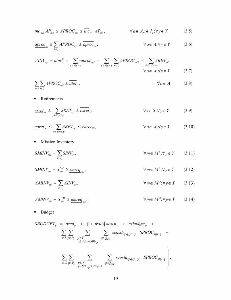
• Ship constraints (3.1) to (3.3) constrain ship procurement: (3.1) ensures that one option for ship procurement is executed yearly at each plant, (3.2) calculates the yearly ship inventory, and (3.3) limits the maximum procurement from each plant.
• (3.4) to (3.8) constrain aircraft procurement: (3.4) to (3.6) guarantee that procurements are made within the limits of one specific segment and without exceeding the general minimum and maximum. (3.7) calculates the yearly aircraft inventory and (3.8) limits the maximum total procurement throughout the years.
• Cumulative retirement goals are specified in (3.9) to (3.10).
• (3.11) to (3.14) keep track of platform inventory to perform each specific mission and then calculate mission shortfalls.
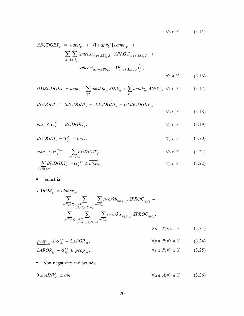
• Budget constraints (3.15) to (3.22) are as follows: (3.15) calculates the ship-budget per year, which depends on the payment profile for each specific ship that has been procured. (3.16) is the yearly aircraft budget, considering the segment cost definition. (3.17) determines O&M costs based on existing inventories. The total yearly budget is assessed in (3.18), which serves to compute deficits and surpluses on a yearly and cumulative basis in (3.19) to (3.22).
• Based on labor profiles for those ships that have been procured, we estimate the labor force level required at the different shipyards in equation (3.23). Then, we compute the lack of labor or excess in (3.24) to (3.25).
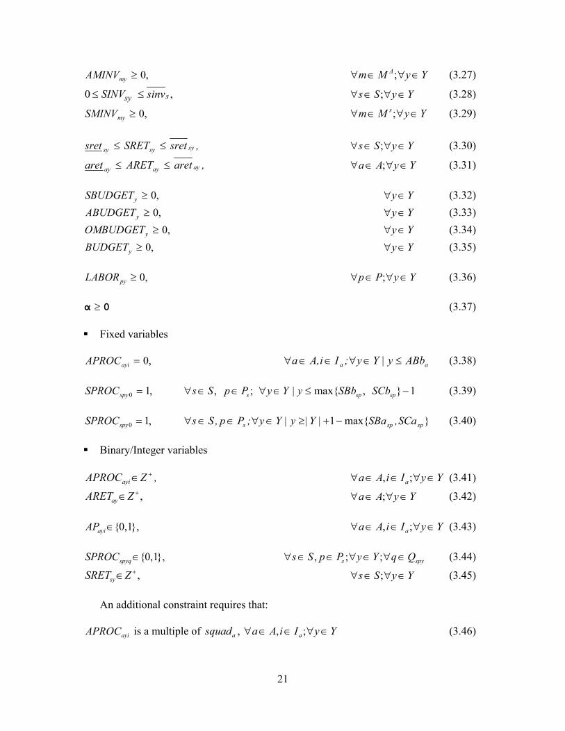
• (3.26) to (3.37) establish non-negativity and bounds for the decision variables. Among these bounds, there exist specified maxima and minima for platform inventory and retirement levels.
• Some variables need to be fixed in (3.38) to (3.39), since otherwise they would involve actions beyond the horizon limits.
22

• (3.41) to (3.45) specify those variables that need to be considered integer or binary. This also implies the integrality of other variables such as platform inventories and mission inventories.
• Finally, (3.46) requires the aircraft procurement to be a multiple of the squadron size. As the remark indicates, this can be accomplished by adding extra segments for those aircraft whose squadron size for procurement purposes is greater than one.
23
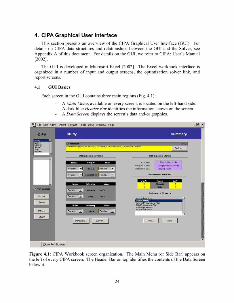
4. CIPA Graphical User Interface This section presents an overview of the CIPA Graphical User Interface (GUI). For
details on CIPA data structures and relationships between the GUI and the Solver, see Appendix A of this document. For details on the GUI, we refer to CIPA: User’s Manual [2002].
The GUI is developed in Microsoft Excel [2002]. The Excel workbook interface is organized in a number of input and output screens, the optimization solver link, and report screens.
4.1 GUI Basics
Each screen in the GUI contains three main regions (Fig. 4.1):
- A Main Menu, available on every screen, is located on the left-hand side. - A dark blue Header Bar identifies the information shown on the screen. - A Data Screen displays the screen’s data and/or graphics.
Figure 4.1: CIPA Workbook screen organization. The Main Menu (or Side Bar) appears onthe left of every CIPA screen. The Header Bar on top identifies the contents of the Data Screenbelow it.
24
From the Main Menu located on the dark-gray bar on the left, we can:
• Access different data screens using the Navigation list boxes. For every screen item selected in the upper box, a subset of subordinate screen items appears in the lower box, and any of these subordinate Data Screens can be displayed.
• Optimize the plan by clicking the Run button. This invokes the Solver. Depending on the problem’s complexity, user settings, and Solver request, the Solver may take just a few seconds, or hours. When the Solver finishes, the new solution is updated on the screen. (Note: Only one Solver run at any one time is permitted, even if several studies are open simultaneously.)
• Switch between a detailed data view and a graphic view using the View Graphics checkbox. This option makes it easier to visualize and understand the data and results.
• Toggle in and out of full-screen mode using the Zoom button.
• Save changes to the study by clicking the Save button. This supports analysis of multiple scenarios and keeps track of the impact that data changes have in the consequent optimal plans.
• Close the study and return Excel to normal mode by clicking the Close button.
25
4.2 Data Screens
We can use any Navigation list box to change the data screen viewed. If a screen has an associated graphic, checking View Graphics on the Main Menu will make this graphic visible. When View Graphics is unchecked, the underlying data is displayed instead. CIPA GUI workbooks contain a variety of data screen types:
• Study Summary: General settings for the Solver and its status.
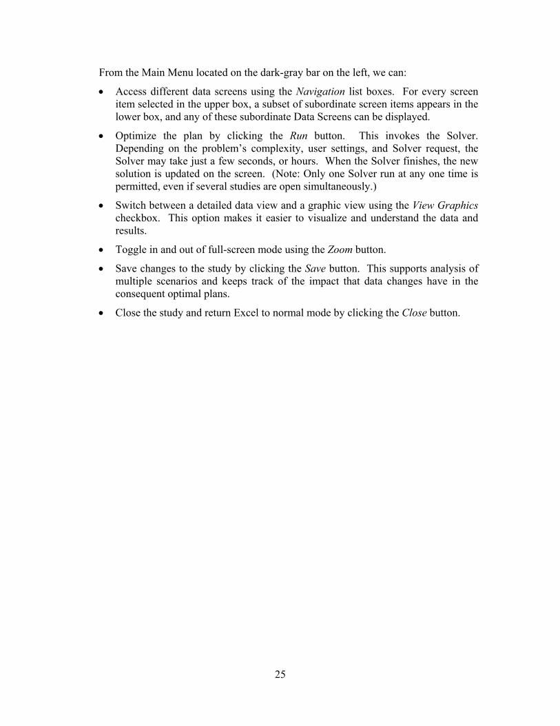
• Budget Summary: Yearly and cumulative budget (available and used).
• Budget Item: Yearly fixed and other cost by category (APN, SCN, O&M) (available and used).
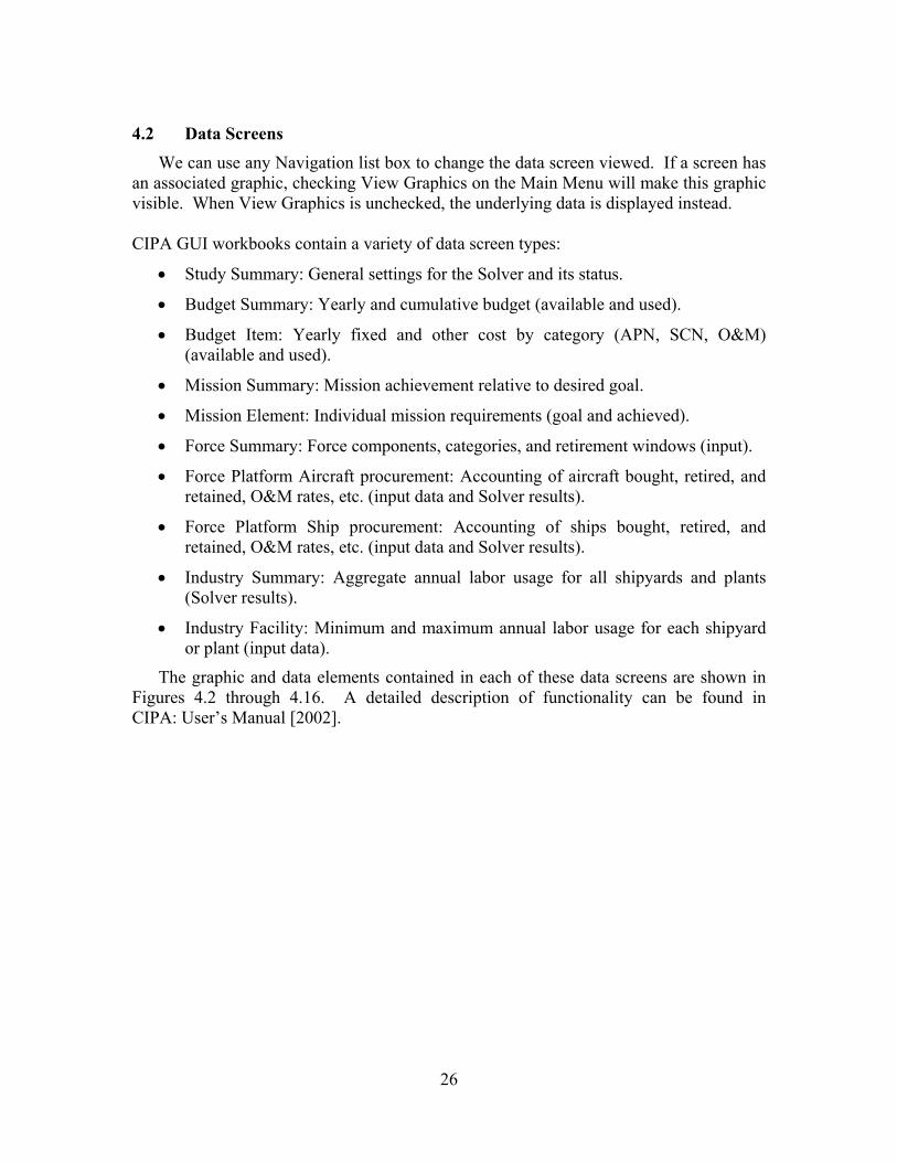
• Mission Summary: Mission achievement relative to desired goal.
• Mission Element: Individual mission requirements (goal and achieved).
• Force Summary: Force components, categories, and retirement windows (input).
• Force Platform Aircraft procurement: Accounting of aircraft bought, retired, and retained, O&M rates, etc. (input data and Solver results).
• Force Platform Ship procurement: Accounting of ships bought, retired, and retained, O&M rates, etc. (input data and Solver results).
• Industry Summary: Aggregate annual labor usage for all shipyards and plants (Solver results).
• Industry Facility: Minimum and maximum annual labor usage for each shipyard or plant (input data).
The graphic and data elements contained in each of these data screens are shown in Figures 4.2 through 4.16. A detailed description of functionality can be found in CIPA: User’s Manual [2002].
26
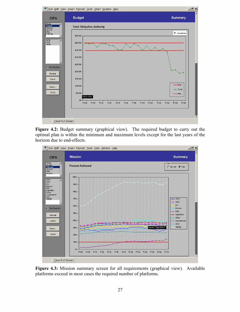
Figure 4.2: Budget summary (graphical view). The required budget to carry out the optimal plan is within the minimum and maximum levels except for the last years of the horizon due to end-effects.
Figure 4.3: Mission summary screen for all requirements (graphical view). Available platforms exceed in most cases the required number of platforms.
27
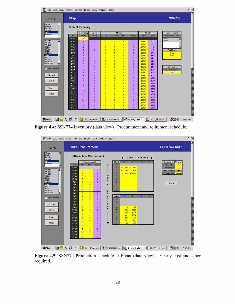
Figure 4.4: SSN774 Inventory (data view). Procurement and retirement schedule.
Figure 4.5: SSN774 Production schedule at Eboat (data view). Yearly cost and labor required.
28
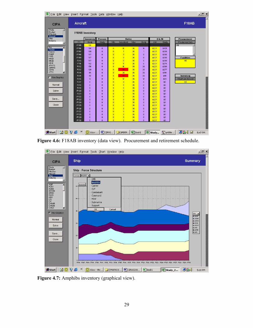
Figure 4.6: F18AB inventory (data view). Procurement and retirement schedule.
Figure 4.7: Amphibs inventory (graphical view).
29
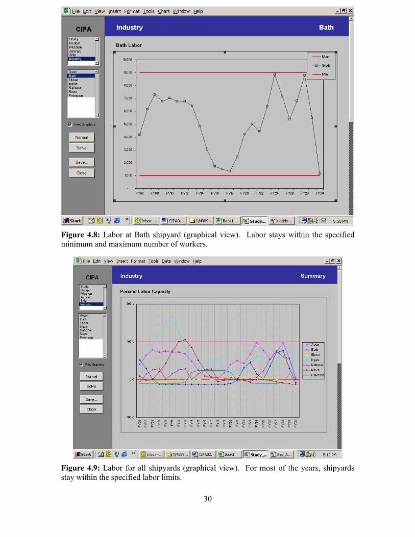
Figure 4.8: Labor at Bath shipyard (graphical view). Labor stays within the specified minimum and maximum number of workers.
Figure 4.9: Labor for all shipyards (graphical view). For most of the years, shipyards stay within the specified labor limits.
30
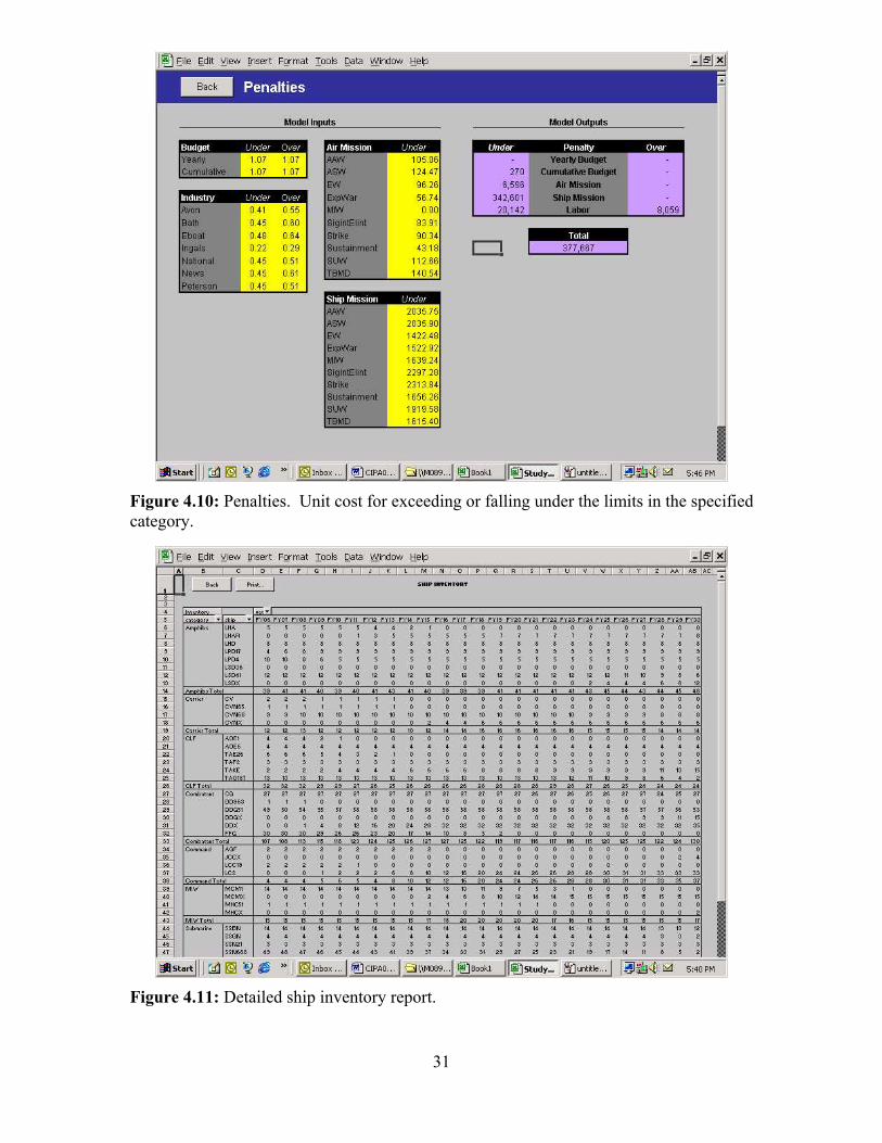
Figure 4.10: Penalties. Unit cost for exceeding or falling under the limits in the specified category.
Figure 4.11: Detailed ship inventory report.
31

Figure 4.12: Detailed air inventory report.
Figure 4.13: Ship procurement plan report.
32

Figure 4.14: Aircraft procurement plan report.
Figure 4.15: SCN expenditure report.
33
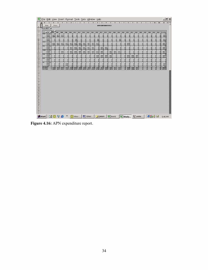
Figure 4.16: APN expenditure report.
34
5. CIPA Solver(s)
5.1 Solvers CIPA has two solvers: The heuristic solver (HS) described in Section 6 and the exact
solver (ES) described in Section 7.
HS is a customized local-search heuristic that finds good solutions quickly. HS also provides a valid lower bound on the optimal solution cost—an objective assessment of the worst-case quality of the solution returned. Because it is very fast, the HS is always executed.
ES uses the commercial algebraic modeling language GAMS [Brooke et al., 1998] to generate a problem instance and then solves it with a contemporary commercial solver (e.g., OSL [GAMS/OSL, 2002], [OSL, 2002], CPLEX [GAMS/CPLEX, 2002], [ILOG, 2002], etc.). ES relaxes the planning problem by treating decisions for aircraft procurement and retirement and ship retirement as continuous, instead of discrete. Moreover, other requirements such as the squadron size for aircraft procurement are not considered. We post-process these solutions (see Section 7) and we provide results of some computation testing in Section 8.
The per-seat software license cost of ES is about $5,000. ES needs to be tended and used by an experienced modeler who can monitor and influence scenario run times, and detect failures. Accordingly, the role of ES is that of a high-cost calibration tool for the fast heuristic solver HS, and perhaps an option to be used selectively to thoroughly investigate and certify finalized scenarios before they are officially published.
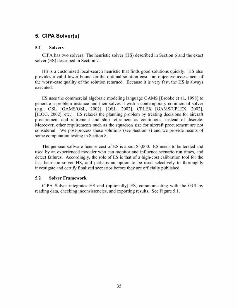
5.2 Solver Framework CIPA Solver integrates HS and (optionally) ES, communicating with the GUI by
reading data, checking inconsistencies, and exporting results. See Figure 5.1.
35

Solver
Data OK? “Data Errors”
Optimize
Optimized? “Errors while Optimizing”
“OptimizationReport”
Read Data
Write Results
End
Verify Data
Y
Y
Figure 5.1: CIPA Solver Flowchart.
36
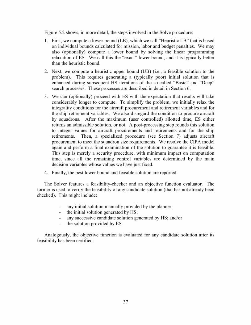
Figure 5.2 shows, in more detail, the steps involved in the Solve procedure:
1. First, we compute a lower bound (LB), which we call “Heuristic LB” that is based on individual bounds calculated for mission, labor and budget penalties. We may also (optionally) compute a lower bound by solving the linear programming relaxation of ES. We call this the “exact” lower bound, and it is typically better than the heuristic bound.
2. Next, we compute a heuristic upper bound (UB) (i.e., a feasible solution to the problem). This requires generating a (typically poor) initial solution that is enhanced during subsequent HS iterations of the so-called “Basic” and “Deep” search processes. These processes are described in detail in Section 6.
3. We can (optionally) proceed with ES with the expectation that results will take considerably longer to compute. To simplify the problem, we initially relax the integrality conditions for the aircraft procurement and retirement variables and for the ship retirement variables. We also disregard the condition to procure aircraft by squadrons. After the maximum (user controlled) allotted time, ES either returns an admissible solution, or not. A post-processing step rounds this solution to integer values for aircraft procurements and retirements and for the ship retirements. Then, a specialized procedure (see Section 7) adjusts aircraft procurement to meet the squadron size requirements. We resolve the CIPA model again and perform a final examination of the solution to guarantee it is feasible. This step is merely a security procedure, with minimum impact on computation time, since all the remaining control variables are determined by the main decision variables whose values we have just fixed.
4. Finally, the best lower bound and feasible solution are reported.
The Solver features a feasibility-checker and an objective function evaluator. The former is used to verify the feasibility of any candidate solution (that has not already been checked). This might include:
- any initial solution manually provided by the planner; - the initial solution generated by HS; - any successive candidate solution generated by HS; and/or - the solution provided by ES.
Analogously, the objective function is evaluated for any candidate solution after its
feasibility has been certified.
37

Optimize
Heuristic LB
End
Exact LB
Heuristic UB
LB on Mission Pen.
LB on Labor Pen.
LB on Budget Pen.
User Options
Solve RMIP
Retrieve Status & Obj. F.
Initial Solution
Basic Search
Deep Search
Exact UB?
Exact UB
User Options
Retrieve Status, Obj. F.
& Solution
Solve MIP Round, Multiple & Fix vars.
Re-Solve MIP Check
Exact UB
Update Best
Best LB (Heur. vs. Exact)
Best UB (Heur. vs. Exact)
Best Solution
Feasibility (Gams Status=2)
Obj. F. match (Gams Status=3)
Y
Figure 5.2: “Optimize” flowchart for the CIPA Solver. The steps involving the exact solver ES are optional.
38
6. CIPA Heuristic In this section, we describe four HS modules: Initial Solution, Basic Search, Deep
Search, and Lower Bound, using notation consistent with the CIPA formulation.
6.1 Initial Solution The first HS step is to find an integer-feasible solution. Because CIPA constraints are
endowed with elastic variables, with linear penalties for violations, it is always possible to assemble an integer-feasible solution, albeit with a lot of penalties.
The initial solution may be a direct user input or a solution found by HS. In the
former case, the user’s solution is checked for feasibility. If feasible, we compute its objective function value and proceed to Heuristic Basic Search. The rest of this section refers to the latter case when the user does not provide an initial solution or when that solution is infeasible.
We construct a myopic initial solution that assigns each variable the minimum value
permitted by the constraints, according to the following scheme: (1) Ship procurement: Produce at each shipyard the minimum amount of each ship
class per year:
YyPpSssprocq
SPROC sspy
spyq ∈∀∈∈∀
=
= ;,,otherwise,0if,1
(2) Aircraft procurement: Procure the minimum feasible number allowed and meet
the squadron size requirement:
- Find, for each and a A∈ y Y∈ : min{ | , ,
such that }ayay
ay aay
ayiayiay a
k k Z k aproc k squad
i I inc k inc
+= ∈ ≥ =
∃ ∈ ≤ ≤
where denotes the condition “k is a multiple of ” ak squad= asquad(Note that typically kay will be zero unless 0
ayaproc > or 1 0ayinc > )
- Assign: APROC, if
0, otherwiseay ay
ayik i i =
=
Yy,Aa ∈∀∈∀
(3) Ship retirement: Retire the minimum of individual and cumulative requirements.
Because cumulative minima in future years may require larger retirements in previous years, we need to first compute the “actual” cumulative minimum retirement implicit in the initial data:
39
- Starting with { }11 1_ : max , ss sActual csret csret sret= , compute
{ }, 1_ : max , _ sysy sy s yActual csret csret Actual csret sret−= +
- Starting at y Y and working backwards, update: | | 1= −
{ }, 1, 1_ : max _ , _ s ysy sy s yActual csret Actual csret Actual csret sret ++= −
- Starting with 1 _ 1s sActual csretSRET = , compute the definite
, 1: _ _sy sySRET Actual csret Actual csrets y−= − (4) Aircraft retirement: Retire the minimum of individual and cumulative
requirements. Because the cumulative minima in future years may require larger retirements in previous years, we need to first compute the “actual” cumulative minimum retirement implicit in the initial data:
- Starting with { }11 1_ : max , aa aActual caret caret aret= , compute
{ }, 1_ : max , _ ayay ay a yActual caret caret Actual caret aret−= +
- Starting at y Y and working backwards, update: | | 1= −
{ }, 1, 1_ : max _ , _ a yay ay a yActual caret Actual caret Actual caret aret ++= −
- Starting with 1 _a 1aARET Actual caret= , compute the definite
, 1: _ _ay ay a yARET Actual caret Actual caret −= −
6.2 Basic Search
The CIPA objective function has three main penalty categories: mission shortfall, budget deficit and surplus, and work-force (industrial) shortfall and excess.
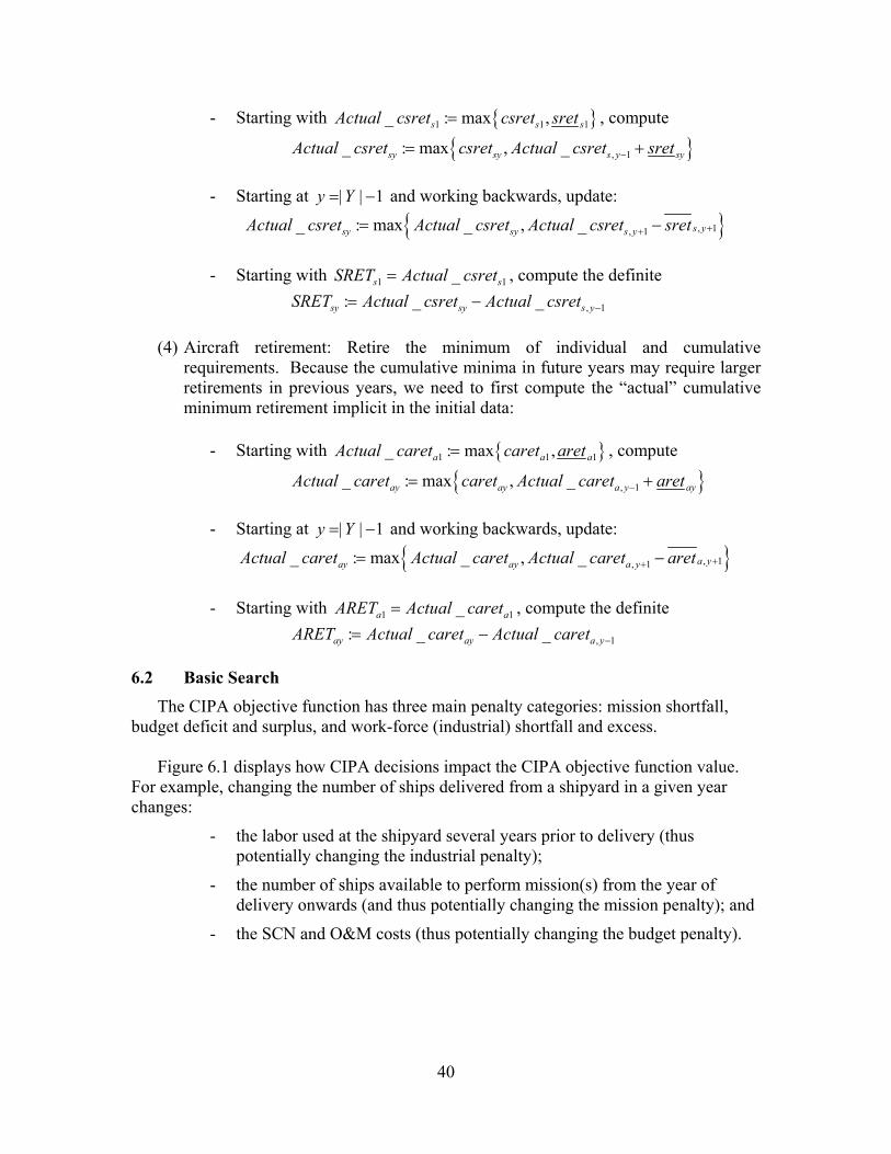
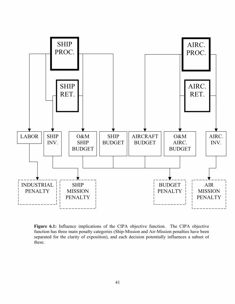
Figure 6.1 displays how CIPA decisions impact the CIPA objective function value.
For example, changing the number of ships delivered from a shipyard in a given year changes:
- the labor used at the shipyard several years prior to delivery (thus potentially changing the industrial penalty);
- the number of ships available to perform mission(s) from the year of delivery onwards (and thus potentially changing the mission penalty); and
- the SCN and O&M costs (thus potentially changing the budget penalty).
40
SHIP PROC.
AIRC.PROC.
SHIPRET.
AIRC.RET.
SHIP BUDGET
O&M SHIP
BUDGET
AIRCRAFTBUDGET
SHIPINV.
AIRC.INV.
LABOR
BUDGET PENALTY
INDUSTRIAL PENALTY
SHIP MISSION PENALTY
AIR MISSION PENALTY
O&M AIRC.
BUDGET
Figure 6.1: Influence implications of the CIPA objective function. The CIPA objectivefunction has three main penalty categories (Ship-Mission and Air-Mission penalties have beenseparated for the clarity of exposition), and each decision potentially influences a subset ofthese.
41

We restrict our analysis to the search for the best possible configuration of a vector x,
where: x=(ship procurement, aircraft procurement, ship retirement, aircraft retirement). We consider our objective function F divided into three components: mission penalty,
budget penalty, and labor penalty. That is, for any feasible solution x:
F(x) = FM(x) + FB(x)+ FL(x)
where FM, FB and FL are the three aforementioned components, respectively. Moreover, the first two terms of the sum can be decomposed as follows:
FM(x) = FSM(x) + FAM(x) and FB(x) = FYB(x) + FCB(x)
where FSM(x) and FAM(x) are the ship-mission and air-mission penalties, and FYB(x) and FCB(x) are the yearly budget and cumulative-budget penalties, respectively.
Our local search seeks feasible solutions that progressively improve the objective function value. We accomplish this by evaluating multiple synchronous modifications to the incumbent configuration, and selecting those that lead to better solutions.
Figure 6.2 shows the basics of the local search procedure. We start with an initial
incumbent solution x*. Then, we apply a number of “Search Strategies” indexed by ss=1,...,SS. Each strategy is characterized by generating a number of tentative solutions, xm , m=1,...,M, located in the “neighborhood” of the current incumbent x*.
Each xm is assigned a ranking position consistent with the strategy, Rss(xm), where a
negative ranking means that the solution is deemed worse that the current x* (whose ranking is zero). Among these candidates, we select the one (say xk) yielding the best ranking. If this improves the current incumbent, we update x* and continue to generate new tentative solutions using the same strategy. If not, we switch to a new strategy to generate the next group of candidates, repeating the process until no strategy produces an improvement.
A straightforward ranking assignment is given by Rss(xm)=F(x*)-F(xm). However, we
will employ other ranking schemes (described later in this document) depending on the strategy ss and on each specific component of the objective function, FSM(x), FAM(x), FYB(x), FCB(x) and FL(x).
The success of Basic Search depends on the strategies applied. We present four strategies that, in practice, have shown a remarkable ability to solve our CIPA model: We call these “Mission,” “Labor,” “Budget,” and “Retirement.”
42
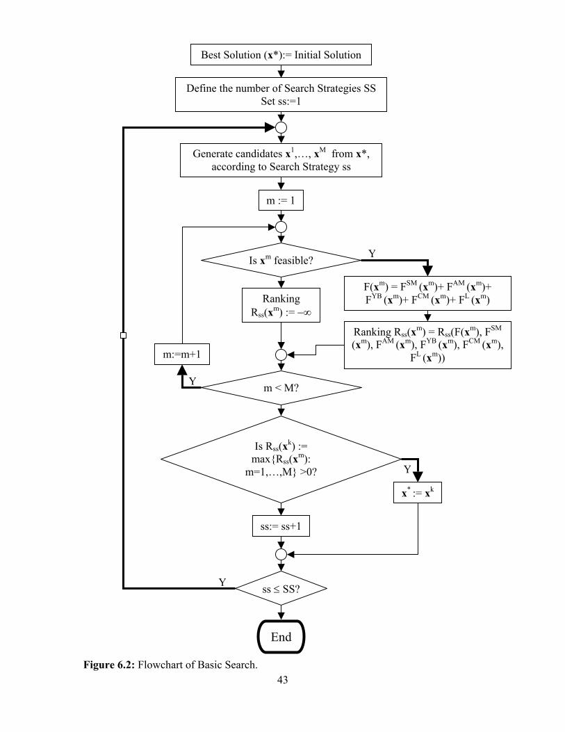
Figure 6.2: Flowchart of Basic Search.
Best Solution (x*):= Initial Solution
Is xm feasible?
Is Rss(xk) := max{Rss(xm):
m=1,…,M} >0?
ss ≤ SS?
End
Define the number of Search Strategies SSSet ss:=1
Generate candidates x1,…, xM from x*, according to Search Strategy ss
m := 1
m:=m+1
m < M?
F(xm) = FSM (xm)+ FAM (xm)+ FYB (xm)+ FCM (xm)+ FL (xm) Ranking
Rss(xm) := −∞
ss:= ss+1
x* := xk
Ranking Rss(xm) = Rss(F(xm), FSM
(xm), FAM (xm), FYB (xm), FCM (xm), FL (xm))
Y
Y
Y
Y
43
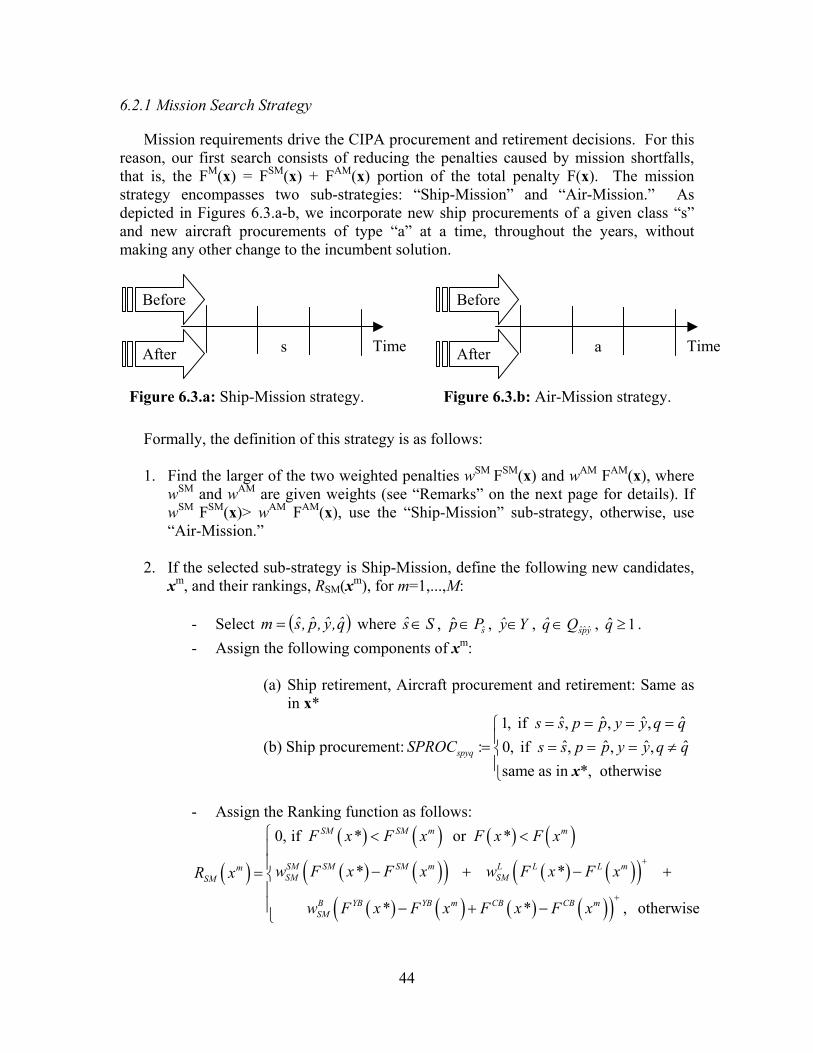
6.2.1 Mission Search Strategy
Mission requirements drive the CIPA procurement and retirement decisions. For this reason, our first search consists of reducing the penalties caused by mission shortfalls, that is, the FM(x) = FSM(x) + FAM(x) portion of the total penalty F(x). The mission strategy encompasses two sub-strategies: “Ship-Mission” and “Air-Mission.” As depicted in Figures 6.3.a-b, we incorporate new ship procurements of a given class “s” and new aircraft procurements of type “a” at a time, throughout the years, without making any other change to the incumbent solution.
Before
After
Figure 6.3.a: Ship-Mission strategy.
s
Time
Before
After
Figure 6.3.b: Air-Mission strategy.
a
Time
Formally, the definition of this strategy is as follows: 1. Find the larger of the two weighted penalties wSM FSM(x) and wAM FAM(x), where
wSM and wAM are given weights (see “Remarks” on the next page for details). If wSM FSM(x)> wAM FAM(x), use the “Ship-Mission” sub-strategy, otherwise, use “Air-Mission.”
2. If the selected sub-strategy is Ship-Mission, define the following new candidates,
xm, and their rankings, RSM(xm), for m=1,...,M:
- Select m where ( q,y,p,s= ) Ss ∈ , ˆˆ sp P∈ , Yy∈ , ypsQq ∈ , q . ˆ 1≥
- Assign the following components of xm:
(a) Ship retirement, Aircraft procurement and retirement: Same as in x*
(b) Ship procurement: SPROCˆ ˆ ˆ1, if , , ,ˆ ˆ ˆ: 0, if , , ,
same as in *, otherwisespyq
s s p p y y q qs s p p y y q q
ˆˆ
= = = == = = = ≠ x
- Assign the Ranking function as follows:
( )( ) ( ) ( ) ( )( ) ( )( ) ( ) ( )( )
( ) ( ) ( ) ( )( )
0, if * or *
* *
* * ,
SM SM m m
SM SM SM m L L L mmSM SMSM
B YB YB m CB CB mSM
F x F x F x F x
w F x F x w F x F xR x
w F x F x F x F x
+
+
< < − + −= − + − otherwise
+
44
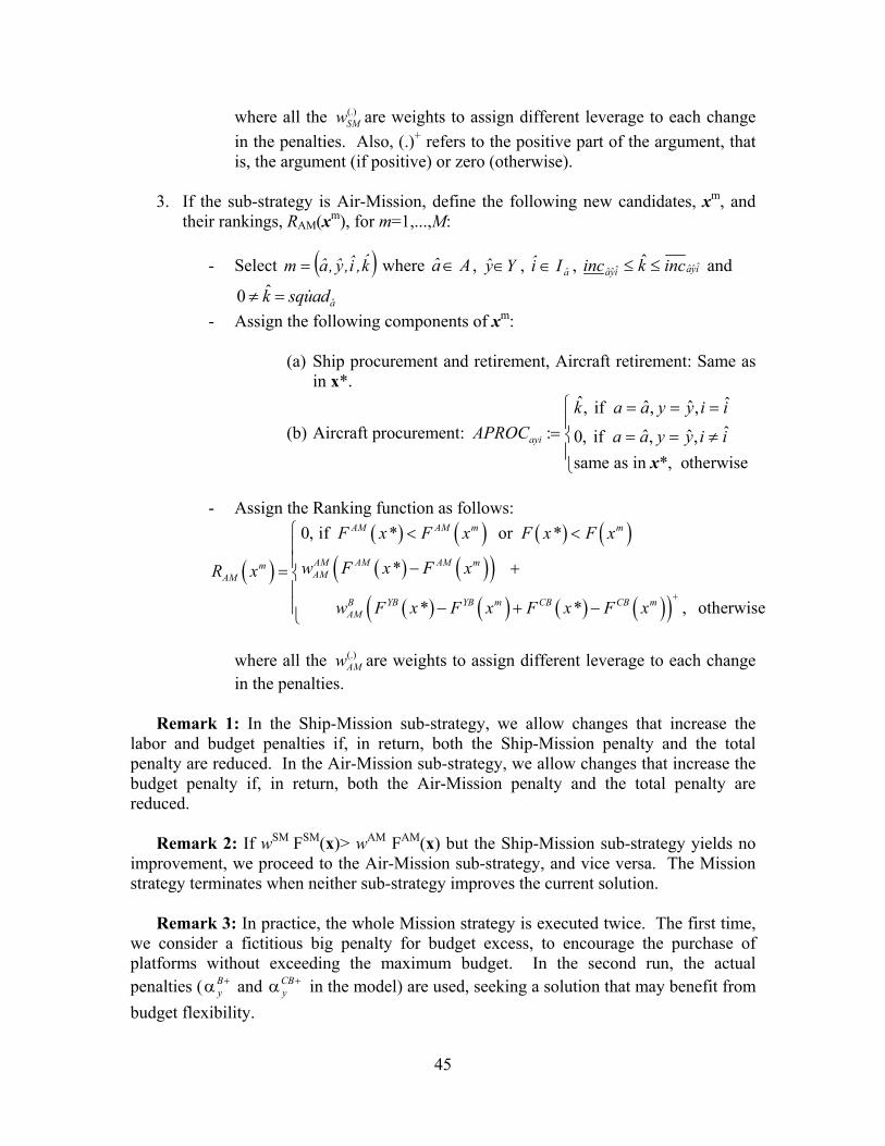
where all the are weights to assign different leverage to each change in the penalties. Also, (.)
(.)SMw
+ refers to the positive part of the argument, that is, the argument (if positive) or zero (otherwise).
3. If the sub-strategy is Air-Mission, define the following new candidates, xm, and
their rankings, RAM(xm), for m=1,...,M:
- Select ( )k,i,y,a=m where Aa ∈ , Yy∈ , i aIˆ ∈ , ˆˆˆˆˆˆˆ ayiayi k inc≤ ≤inc and
asquadˆ0 k≠ =- Assign the following components of xm:
(a) Ship procurement and retirement, Aircraft retirement: Same as in x*.
(b) Aircraft procurement:
ˆ ˆˆ ˆ, if , ,ˆ: ˆ ˆ0, if , ,
same as in *, otherwiseayi
k a a y y i iAPROC a a y y i i
= = =
= = = ≠ x
- Assign the Ranking function as follows:
( )( ) ( ) ( ) ( )( ) ( )( )
( ) ( ) ( ) ( )( )
0, if * or *
*
* * ,
AM AM m m
AM AM AM mmAMAM
B YB YB m CB CB mAM
F x F x F x F x
w F x F xR x
w F x F x F x F x+
< < − += − + − otherwise
where all the are weights to assign different leverage to each change in the penalties.
(.)AMw
Remark 1: In the Ship-Mission sub-strategy, we allow changes that increase the
labor and budget penalties if, in return, both the Ship-Mission penalty and the total penalty are reduced. In the Air-Mission sub-strategy, we allow changes that increase the budget penalty if, in return, both the Air-Mission penalty and the total penalty are reduced.
Remark 2: If wSM FSM(x)> wAM FAM(x) but the Ship-Mission sub-strategy yields no
improvement, we proceed to the Air-Mission sub-strategy, and vice versa. The Mission strategy terminates when neither sub-strategy improves the current solution.
Remark 3: In practice, the whole Mission strategy is executed twice. The first time,
we consider a fictitious big penalty for budget excess, to encourage the purchase of platforms without exceeding the maximum budget. In the second run, the actual penalties ( and in the model) are used, seeking a solution that may benefit from budget flexibility.
+αBy
+αCBy
45
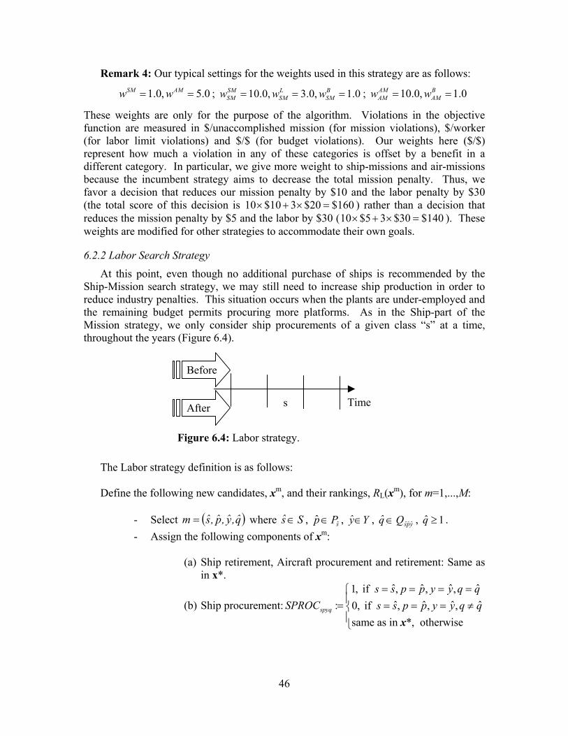
Remark 4: Our typical settings for the weights used in this strategy are as follows:
1.0, 5.0SM AMw w= = ; ; 10.0, 3.0, 1.0SM L BSM SM SMw w w= = = 10.0, 1.0AM B
AM AMw w= =
These weights are only for the purpose of the algorithm. Violations in the objective function are measured in $/unaccomplished mission (for mission violations), $/worker (for labor limit violations) and $/$ (for budget violations). Our weights here ($/$) represent how much a violation in any of these categories is offset by a benefit in a different category. In particular, we give more weight to ship-missions and air-missions because the incumbent strategy aims to decrease the total mission penalty. Thus, we favor a decision that reduces our mission penalty by $10 and the labor penalty by $30 (the total score of this decision is 10 $10 3 $20 $160× + × = ) rather than a decision that reduces the mission penalty by $5 and the labor by $30 (10 $5 3 $30 $140× + × = ). These weights are modified for other strategies to accommodate their own goals.
6.2.2 Labor Search Strategy
At this point, even though no additional purchase of ships is recommended by the Ship-Mission search strategy, we may still need to increase ship production in order to reduce industry penalties. This situation occurs when the plants are under-employed and the remaining budget permits procuring more platforms. As in the Ship-part of the Mission strategy, we only consider ship procurements of a given class “s” at a time, throughout the years (Figure 6.4).
Before
After
Figure 6.4: Labor strategy.
s
Time
The Labor strategy definition is as follows:
Define the following new candidates, xm, and their rankings, RL(xm), for m=1,...,M:
- Select m where ( q,y,p,s= ) Ss ∈ , ˆˆ sp P∈ , Yy∈ , ypsQq ∈ , q . ˆ 1≥- Assign the following components of xm:
(a) Ship retirement, Aircraft procurement and retirement: Same as in x*.
(b) Ship procurement:ˆ ˆ ˆ1, if , , ,ˆ ˆ ˆ: 0, if , , ,
same as in *, otherwisespyq
s s p p y y q qSPROC s s p p y y q q
ˆˆ
= = = == = = = ≠ x
46
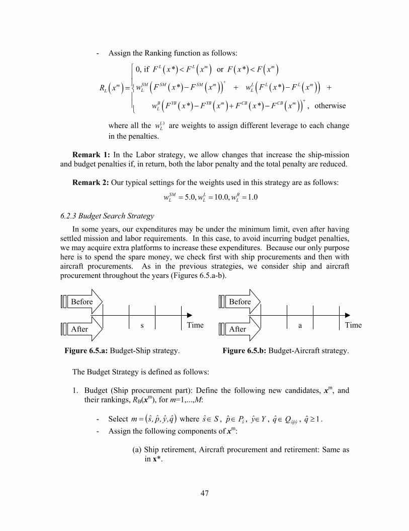
- Assign the Ranking function as follows:
( )( ) ( ) ( ) ( )
( ) ( )( ) ( ) ( )( )( ) ( ) ( ) ( )( )
0, if * or *
* *
* * ,
L L m m
SM SM SM m L L L mmL LL
B YB YB m CB CB mL
F x F x F x F x
w F x F x w F x F xR x
w F x F x F x F x
+
+
< < − + −= − + − otherwise
+
)
where all the are weights to assign different leverage to each change in the penalties.
(.)Lw
Remark 1: In the Labor strategy, we allow changes that increase the ship-mission
and budget penalties if, in return, both the labor penalty and the total penalty are reduced. Remark 2: Our typical settings for the weights used in this strategy are as follows:
5.0, 10.0, 1.0SM L BL L Lw w w= = =
6.2.3 Budget Search Strategy
In some years, our expenditures may be under the minimum limit, even after having settled mission and labor requirements. In this case, to avoid incurring budget penalties, we may acquire extra platforms to increase these expenditures. Because our only purpose here is to spend the spare money, we check first with ship procurements and then with aircraft procurements. As in the previous strategies, we consider ship and aircraft procurement throughout the years (Figures 6.5.a-b).
Before
After
Figure 6.5.a: Budget-Ship strategy.
s
Time
Before
After
Figure 6.5.b: Budget-Aircraft strategy.
a
Time
The Budget Strategy is defined as follows:
1. Budget (Ship procurement part): Define the following new candidates, xm, and
their rankings, RB(xm), for m=1,...,M:
- Select m where ( q,y,p,s= Ss ∈ , ˆˆ sp P∈ , Yy∈ , ypsQq ∈ , q . ˆ 1≥
- Assign the following components of xm:
(a) Ship retirement, Aircraft procurement and retirement: Same as in x*.
47

(b) Ship procurement:ˆ ˆ ˆ1, if , , ,ˆ ˆ ˆ: 0, if , , ,
same as in *, otherwisespyq
s s p p y y q qSPROC s s p p y y q q
ˆˆ
= = = == = = = ≠ x
- Assign the Ranking function as follows:
( )( ) ( ) ( ) ( ) ( ) ( )
( ) ( ) ( ) ( )0, if * * + or *
* * , otherwise
YB CB YB m CB m m
mB YB YB m CB CB m
F x F x F x F x F x F xR x
F x F x F x F x
+ < <= − + −
2. Budget (Aircraft procurement part): Define the following new candidates, xm, and
their rankings, RB(xm), for m=1,...,M:
- Select ( )k,i,y,a=m where Aa ∈ , Yy∈ , aIi ∈ , ˆˆˆˆˆˆˆ ayiayiinc k inc≤ ≤ and
. asquadˆ0 k≠ =- Assign the following components of xm:
(a) Ship procurement and retirement, Aircraft retirement: Same as in x*.
(b) Aircraft procurement:
ˆ ˆˆ ˆ, if , ,ˆ: ˆ ˆ0, if , ,
same as in *, otherwiseayi
k a a y y i iAPROC a a y y i i
= = =
= = = ≠ x
- Assign the ranking function as follows:
( )( ) ( ) ( ) ( ) ( ) ( )
( ) ( ) ( ) ( )0, if * * + or *
* * , otherwise
+ < <= − + −
YB CB YB m CB m m
mB YB YB m CB CB m
F x F x F x F x F x F xR x
F x F x F x F x
Remark: The ranking function RB is the same for the ship and aircraft stages of the
budget search strategy. We only allow changes that reduce both the budget penalty and the total penalty.
6.2.4 Retirement Search Strategy
The initial retirement schedule follows minimum retirements from the input data (which may be zero), disregarding how new procurements should influence earlier retirements of obsolete or redundant assets. The Retirement Strategy assesses the tradeoff between earlier platform retirements (which reduces O&M costs) and Ship-Mission accomplishment. The analysis is done for ships first, and then for aircraft (Figures 6.6.a-b).
48
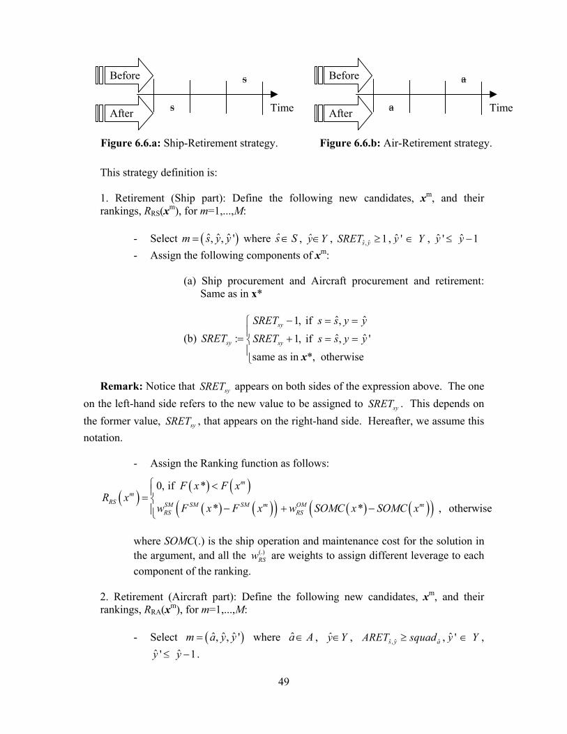
Before
After
Figure 6.6.a: Ship-Retirement strategy.
s
s
Time
Before
After
Figure 6.6.b: Air-Retirement strategy.
a
a
Time
This strategy definition is: 1. Retirement (Ship part): Define the following new candidates, xm, and their rankings, RRS(xm), for m=1,...,M:
- Select m s where ( ˆ ˆ ˆ, , 'y y= ) Ss ∈ , Yy∈ , ,ˆ ˆ, 1s ySRET ≥ ˆ 'y Y∈ , ˆ ˆ' 1y y≤ − - Assign the following components of xm:
(a) Ship procurement and Aircraft procurement and retirement: Same as in x*
(b) SRET
ˆ ˆ1, if ,ˆ ˆ: 1, if , '
same as in *, otherwise
sy
sy sy
SRET s s y ySRET s s y y
− = == + = = x
Remark: Notice that sySRET appears on both sides of the expression above. The one
on the left-hand side refers to the new value to be assigned to sySRET . This depends on the former value, sySRET , that appears on the right-hand side. Hereafter, we assume this notation.
- Assign the Ranking function as follows:
( )( ) ( )
( ) ( )( ) ( ) ( )( )0, if *
* *
m
mRS SM SM SM m OM m
RS RS
F x F xR x
w F x F x w SOMC x SOMC x
<= − + − , otherwise
)
where SOMC(.) is the ship operation and maintenance cost for the solution in the argument, and all the are weights to assign different leverage to each component of the ranking.
(.)RSw
2. Retirement (Aircraft part): Define the following new candidates, xm, and their rankings, RRA(xm), for m=1,...,M:
- Select m a where ( ˆ ˆ ˆ, , 'y y= a A∈ , Yy∈ , ˆ ˆ ˆ,s y aARET squad≥ , ˆ 'y Y∈ ,
ˆ ˆ' 1y y≤ − .
49
- Assign the following components of xm:
(a) Ship procurement, Aircraft procurement and retirement: Same as in x*.
(b) Ship retirement:
ˆ ˆ, if ,ˆ ˆ: , if , '
same as in *, otherwise
ay a
ay ay a
ARET squad a a y yARET ARET squad a a y y
− = == + = = x
- Assign the Ranking function as follows:
( )( ) ( )
( ) ( )( ) ( ) ( )( )0, if *
* *
m
mRA AM AM AM m OM m
RA R
F x F xR x
w F x F x w AOMC x AOMC x
<= − + − , otherwise
where AOMC(.) is the aircraft operation and maintenance cost for the solution in the argument, and all the are weights to assign different leverage to each component of the ranking.
(.)RAw
Remark 1: We allow changes that may increase the ship and air mission penalties if,
in return, the total penalty is reduced. Remark 2: In practice, we use this strategy before and after each of the other
strategies (Mission, Labor, and Budget). This permits retirements to keep pace as the Basic Search updates procurements.
Remark 3: Our typical settings for the weights used in this strategy are:
1.0, 1.0SM OMRS RSw w= = ; 1.0, 1.0AM OM
RA RAw w= =
6.3 Deep Search In Basic Search, we explore new solutions that differ from the best incumbent
solution in only one component. In Retirement Search, each change affects two components, with a retirement moved earlier. Note, however, that each change involves just one platform type at a time.
The Basic Search strategy is preserved, in part, during Deep Search: We continue to
list a number of candidate moves and select the one with the best ranking. However, Deep Search provides a broader spectrum of configurations to analyze in hopes of overcoming the myopia of Basic Search. Theoretically, Deep Search can implement any conceivable move, whether it consists of a single change in the components or combines multiple changes.
50
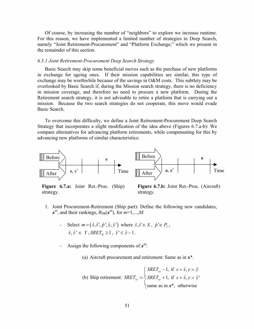
Of course, by increasing the number of “neighbors” to explore we increase runtime. For this reason, we have implemented a limited number of strategies in Deep Search, namely “Joint Retirement-Procurement” and “Platform Exchange,” which we present in the remainder of this section.
6.3.1 Joint Retirement-Procurement Deep Search Strategy Basic Search may skip some beneficial moves such as the purchase of new platforms
in exchange for ageing ones. If their mission capabilities are similar, this type of exchange may be worthwhile because of the savings in O&M costs. This subtlety may be overlooked by Basic Search if, during the Mission search strategy, there is no deficiency in mission coverage, and therefore no need to procure a new platform. During the Retirement search strategy, it is not advisable to retire a platform that is carrying out a mission. Because the two search strategies do not cooperate, this move would evade Basic Search.
To overcome this difficulty, we define a Joint Retirement-Procurement Deep Search
Strategy that incorporates a slight modification of the idea above (Figures 6.7.a-b): We compare alternatives for advancing platform retirements, while compensating for this by advancing new platforms of similar characteristics:
Before
After
Figure 6.7.b: Joint Ret.-Proc. (Aircraft)strategy.
a, a’
a
Time
Before
After
Figure 6.7.a: Joint Ret.-Proc. (Ship)strategy.
s, s’
s
Time
1. Joint Procurement-Retirement (Ship part): Define the following new candidates,
xm, and their rankings, RPR(xm), for m=1,...,M:
- Select m s where ( )ˆ ˆ ˆ ˆ ˆ, ', ', , 's p y y= ˆ ˆ, 's s S∈ , ˆ 'ˆ ' sp P∈ , ˆ ˆ, 'y y Y∈ ˆˆ 1sySRET ≥, , ˆ ˆ' 1y y≤ − .
- Assign the following components of xm:
(a) Aircraft procurement and retirement: Same as in x*.
(b) Ship retirement: SRET
ˆ ˆ1, if ,ˆ ˆ: 1, if , '
same as in *, otherwise
sy
sy sy
SRET s s y ySRET s s y y
− = == + = = x
51

(c) Ship procurement: ' ' ' 1
' ' '
ˆ ˆ ˆ1, if ', ', ', 1ˆ ˆ ˆ: 0, if ', ', ', 1
same as in *, otherwise
s p y q
spyq s p y q
s s p p y y SPROCSPROC s s p p y y SPROC
−= = ==
=
= = = = x
- Assign the Ranking function as follows:
( )( ) ( )
( ) ( )0, if *
* , otherwise
m
mJR m
F x F xR x
F x F x
<= −
2. Joint Procurement-Retirement (Aircraft part): Define the following new
candidates, xm, and their rankings, RPR(xm), for m=1,...,M:
- Select m a where ( )ˆ ˆ ˆ ˆ, ', , 'a y y= ˆ ˆ, 'a a A∈ , ˆ ˆ, 'y y Y∈ , ˆˆ ˆsy aSRET squad≥ , ˆ ˆ' 1y y≤ − .
- Let i be such that ˆˆ ', 'k
ˆ ˆ'
ˆˆ ˆ' ' 'ˆ ˆˆ ˆˆ ' ' '' ˆ ˆ' ' '
ˆ ' min{ | , k , ˆ ' such that }
a a
a y ia y ia a y i
k k Z k squad squad
i I inc APROC k inc
+= ∈ = ≥
∃ ∈ ≤ + ≤
(Remark: If do not exist, then the move is infeasible) ˆˆ ', 'i k - Assign the following components of xm:
(a) Ship procurement and retirement: Same as in x*. (b) Aircraft procurement:
ˆ ˆˆ ˆ', if ', ', ': ˆˆ ˆ0, if ', ', '
same as in *, otherwise
ayi
ayi
APROC k a a y y i iAPROC a a y y i i
+ = = =
= = = ≠ x
(c) Aircraft retirement: ˆ
ˆ
ˆ ˆ, if ,ˆ ˆ: , if , '
same as in *, otherwise
ay a
ay ay a
ARET squad a a y yARET ARET squad a a y y
− = == + = = x
- Assign the Ranking function as follows:
( )( ) ( )
( ) ( )0, if *
* , other
<= −
m
mJR m
F x F xR x
F x F x wise
52

6.3.2 Platform Exchange Deep Search Strategy Exchange strategies refer to tentative moves involving the exchange of one platform
procurement with another, but not necessarily in the same year, and not necessarily of the same type.
We have analyzed different ways to check for platform exchanges (Figures 6.8.a-d):
In “Ship Exchange,” we exchange the years that two different ships are procured; in “Aircraft Exchange,” we exchange the years that two different aircraft are procured; in “Ship-Aircraft Exchange” we evaluate exchanges of a ship purchase with an aircraft purchase; and in “Plant Exchange” we exchange a ship purchase from a specific shipyard and year with the same ship class purchased from a different shipyard and/or year.
Before
After
Figure 6.8.b: Aircraft Exchange.
a’
a
a
a’
Time
Before
After
Figure 6.8.a: Ship Exchange.
s’
s
s
s’
Time
Before
After
Figure 6.8.c: Ship-Aircraft Exchange.
(a)
s
(a)
Time
Before
After
Figure 6.8.d: Ship-Plant Exchange.
(s,p’)
s,p
(s,p’)
Time
Formal definitions are as follows: 1. Platform-Exchange (Ship part): Define the following new candidates, xm, and
their rankings, RPES(xm), for m=1,...,M:
- Select m s where ( )ˆ ˆ ˆ ˆ ˆ ˆ, , ', ', , 'p s p y y= ˆ ˆ, 's s S∈ , ˆˆ sp P∈ , ˆ 'ˆ ' sp P∈ , ˆ ˆ, 'y y Y∈ ˆˆ ˆˆ 0 | spyqq SPROC, ∃ ≠ , ˆ 1= ˆˆPROC ˆ ˆ ' 1spyqˆ ' 0 |q S∃ ≠ = .
- Assign the following components of xm:
(a) Aircraft procurement and retirement, and ship retirement: Same as in x*.
53

(b) Ship procurement: ', 1
'
, 1
' ' , 1
ˆ ˆ ˆ1, if , , ', 1ˆ ˆ ˆ0, if , , ', 1ˆ ˆ ˆ1, if , , , 1ˆ ˆ ˆ0, if , , , 1ˆ ˆ ˆ: 1, if ', ', , 1
0, if
spy q
spy q
spy q
spyq
spyq s p y q
s s p p y y SPROC
s s p p y y SPROCs s p p y y SPROCs s p p y y SPROC
SPROC s s p p y y SPROC
−
+
−
= = = =
= = = =
= = = =
= = = =
= = = = =
' '
' ' ', 1
' ' '
ˆ ˆ ˆ', ', , 1ˆ ˆ ˆ1, if ', ', ', 1ˆ ˆ ˆ0, if ', ', ', 1
same as in *, otherwise
s p yq
s p y q
s p y q
s s p p y y SPROCs s p p y y SPROC
s s p p y y SPROC+
= = = = = = = =
= = = = x
- Assign the Ranking function as follows:
( )( ) ( )
( ) ( )0, if *
* , other
<= −
m
mRES m
F x F xR x
F x F x wise
2. Platform-Exchange (Aircraft part), Platform-Exchange (Ship-Aircraft part), and Platform-Exchange (Plant part) are defined in a similar fashion.
6.4 Heuristic Lower Bound
Computing a good-quality lower bound (LB) by data inspection is not a trivial task. No feasible solution can have a better objective function value than the specified LB:
( ), feasible.≤ ∀LB F x x
CIPA constructs a lower bound by separately bounding each component of the
separable objective function:
F(x) = FSM(x) + FAM(x) + FYB(x) + FCB(x) + FL(x).
We will compute the following LBs: , , , , ,
( )SM SMLB F x≤feasible
( )AM AMLB F x≤( )YB YBLB F x≤ ( )CB CBLB F x≤ ( )L LLB F x≤ x∀ . Then, it is clear that:
( ), feasibleSM AM YB CB LLB LB LB LB LB LB F x x= + + + + ≤ ∀ .
We now describe how to calculate each of these individual LBs.
54
6.4.1 Lower Bound on Ship-Mission Penalty
The question is: “Can we establish any ship-mission shortfall by data inspection?” To be able to answer this question, we:
(a) Compute the actual maximum ship inventory for every ship class, s, and year y.
(b) Compute the minimum penalty incurred by ships due to lack of resources to accomplish the required Ship-Missions.
We must realize that part (a) above is not immediate. There are several factors conditioning the maximum possible inventory of a specific class s in year y:
- The initial inventory, 0ssi . nv
- The maximum inventory specified by the user, ssinv . - The ongoing committed production, sycsproc . - The maximum and minimum procurement per year from each plant,
spysproc , spy
sproc .
- The maximum total procurement from each plant, spstot . - The production and payment schedule at each plant (and, therefore, the
earliest that ships can be acquired), spSBb , spSCb . - And finally, the minimum yearly and cumulative retirements imposed by
the user, sysret , sycsret .
Each of the seven factors above may influence the maximum possible inventory of ships. Moreover, data for future years may influence the maximum inventory in earlier years. For example, meeting minimum cumulative retirements in the future may require retiring ships earlier, which in turn reduces the maximum inventory. The minimum procurement influences the maximum inventory: Because there is a maximum total procurement, if a minimum procurement exists in the future, then the maximum inventory in the present will be reduced. For example, if the maximum procurement over the time horizon is three ships and the minimum in the second year is one ship, then, in the first year, we cannot procure more than two ships.
Now, we present an overview of how the LBSM bound is computed:
(1) Using the yearly and cumulative retirements, sysret , sycsret , update
the minimum cumulative retirement, CUM_SretMin(s,y): _ ( , ) : max{ _ ( , -1) , }.= + sy syCum SRetMin s y Cum SRetMin s y sret csret
55

(2) Using the committed procurement, sycsproc , calculate the cumulative committed procurements, Cum_CSProc(s,y):
_ ( , ) _ ( , -1)= + .∑ spyp
Cum CSProc s y Cum CSProc s y csproc
(3) Calculate the new maximum ship inventory, Max_SInv(s,y):
( )0_ ( , ) : _ ( , ) _ ( , ) .= − + −s sMax SInv s y sinv sinv Cum CSProc s y Cum SRetMin s y (4) Calculate (working backwards in time) the adjusted maximum ship
inventory, Adj_Max_SInv(s,y): _ _ ( , ) : min{ _ ( , ), _ _ ( , 1)}.= +Adj Max SInv s y Max SInv s y Adj Max SInv s y
(5) Calculate the maximum total ships to be procured, Max_Stot(s,p,y).
Starting with _ ( , ,| |) spMax Stot s p Y stot= , work backwards in time:
, 1_ ( , , ) _ ( , , 1) .
+= + −
sp yMax Stot s p y Max Stot s p y sproc
(6) Calculate the initial maximum cumulative procurement that can be
procured from each plant, Ini_Cum_MaxProc(s,p,y):
'1 '
_ _ ( , , )≤ ≤
= .∑ spyy y
Ini Cum MaxProc s p y sproc
and the first index y where this amount exceeds the maximum per plant: ˆ min{ | _ _ ( , , ) _ ( , , )}y y Ini Cum MaxProc s p y Max STot s p y= >
= ∞ _ ( , , ) _ ( , , ),um axProc s p y Max STot s p y y
(or if Cy M ≤ ∀ ) (7) Calculate the adjusted maximum procurement, MaxSProc(s,p,y):
0, if max{ 1, 1}
ˆ, if max{ , }( , , ) : .ˆ_ ( , , ) _ _ ( , , 1), if
ˆ0, if
< + +
≤ <= − − =
>
sp sp
sp spspy
y SBb SCb
sproc SBb SCb y yMaxProc s p yMax STot s p y Ini Cum MaxProc s p y y y
y y
(8) Accrue procurements from all plants, All_MaxSProc(s,y):
_ ( , ) : ( ,= , ).∑p
All MaxProc s y MaxProc s p y
and calculate the cumulative amounts, Cum_All_MaxSProc(s,y):
1 '_ _ ( , ) _ ( ,
≤ ≤
= ').∑y y
Cum All MaxProc s y All MaxProc s y
56
(9) Compare with the adjusted maximum ship inventory: _ _ ( , ) min{ _ _ ( , ), _ _ ( , )}.=Cum All MaxProc s y Cum All MaxProc s y Adj Max SInv s y
(10) Calculate an upper bound on the maximum inventory of ships:
0_ ( , ) : _ ( , ) _ ( , ) ._ _ ( , )
= + −sUB SInv s y sinv Cum CSProc s y Cum SRetMin s yCum All MaxProc s y
+
).
(11) Calculate the inventory upper bound per Ship-Mission:
_ ( , ) _ ( ,∈
= ∑ms S
UB MInv m y UB SInv s y
(12) Calculate the lower bound on the penalty per year and Ship-Mission:
( , ) max{0, ( _ ( , ))};= −m myLB m y smpen smreq UB MInv m y
and the total bound on Ship-Mission penalty:
( , )∈∈
= ∑ ∑S
SM
y Ym M
LB LB m y .
+
6.4.2 Lower Bound on Air-Mission Penalty
A lower bound on Air-Mission penalty can be obtained in an analogous fashion to the lower bound on Ship-Mission penalty. The differences in the procedure are summarized as follows:
(a) There is no need to perform individual plant calculations.
(b) The minimum year to produce an aircraft is , instead of as used in Step (7) of the ship procedure.
1aABb +max{ 1, 1}sp spSBb SCb+
(c) When calculating the maximum procurement per year, squadron sizes and segments for aircraft must be taken into account.
6.4.3 Lower Bound on Labor Penalty
A labor penalty arises when labor exceeds the maximum level or falls below the minimum level at any plant. We can derive a lower bound on these penalties.
This is an overview of how the LBL bound is computed:
(1) Update the minimum and maximum amounts of ships that can be
procured:
,sprocspy
0= 1-}max{ spsps SCb,SBby;Pp,Ss ≤∀∈∈∀ , and
,sprocspy
0= }spmax{1 sps SCa,SBa|Y|y;Pp,Ss −+≥∀∈∈∀ ;
57
,sprocspy 0= 1-}max{ spsps SCb,SBby;Pp,Ss ≤∀∈∈∀ and
,sprocspy 0= }spmax{1 sps SCa,SBa|Y|y;Pp,Ss −+≥∀∈∈∀ .
(2) Compute the yearly minimum and maximum possible labor per plant, Min_Labor(p,y), Max_Labor(p,y) according to production schedules and required minimum and maximum quantities, YyPp ∈∀∈∀ ; :
'
'
, , '| ' |
'
, , '| ' |
' 1
_ ( , )
spys
sp
spys
sp
py
sp sproc y ys S p P y Y
y y y SCb
sp sproc y ys S p P y Y
y SCa y y
Min LABOR p y clabor
sworkb
sworka
−∈ ∈ ∈
≤ ≤ +
−∈ ∈ ∈
− ≤ ≤ −
= +
+∑ ∑
∑ ∑
'
'
, , '| ' |
'
, , '| ' |
' 1
_ ( , )
.
−∈ ∈ ∈
≤ ≤ +
−∈ ∈ ∈
− ≤ ≤ −
= +
+∑ ∑
∑ ∑
spys
sp
spys
sp
py
sp sproc y ys S p P y Y
y y y SCb
sp sproc y ys S p P y Y
y SCa y y
Max LABOR p y clabor
sworkb
sworka
(3) Compute the yearly penalties for violating the minimum and maximum limits per plant, YyPp ∈∀∈∀ ; :
( , ) max{0, _ ( , )}Lp py
LB p y lpen pcap Max LABOR p y− −= −
( , ) max{0, _ ( , ) }.+ += −Lp pyLB p y lpen Min LABOR p y pcap
(4) Compute a lower bound on labor cost due to under-employment, LBL-,
a lower bound on labor cost due to labor excess, LBL+, and the total lower bound on labor cost, LBL:
( , )L L
y Y p P
LB LB− −
∈ ∈
= p y∑∑
( , )L L
y Y p P
LB LB+ +
∈ ∈
= p y∑∑
.− += +L L LLB LB LB
6.4.4 Lower Bound on Budget Penalty
A budget penalty applies when the expenditures in a given year exceed the maximum budget or fall below the minimum budget. Currently, a lower bound of zero is considered for both penalties, LBB+ =0 and LBB- =0, respectively.
58

We could calculate lower bounds by analyzing
(a) the maximum possible procurement and O&M cost (to compute a better LBB-), and
(b) the minimum possible procurement cost (to compute a better LBB+).
However, it is unlikely that these bounds render non-zero values because
(a) it is clear that we will be able, in general, to expend more than the minimum budget, and
(b) we do not expect that the minimum feasible purchase already exceeds the maximum budget, since that problem would be unrealistic under the present conditions.
However, we continue to seek other bounds for missions, labor and budget, as well as bounds that do not rely on individually bounding each of these penalties.
59

7. Features of the Exact Algorithm Exact Solver (ES) implements a simplified version of the CIPA model in GAMS, and
then uses commercial optimization software (e.g., CPLEX, OSL) to solve it. The ES also produces a lower bound on the optimal solution of the problem.
In this section, we detail the calculation of the lower and upper bounds through the
ES.
7.1 Lower Bound Any relaxation of the CIPA model constraints produces a new model whose optimal
solution is no worse (i.e., it has objective function value no greater) than the optimal solution of the original CIPA model. The goal is to find a relaxed model that is easy to solve and yields a good bound (i.e., close to the optimal solution of the original problem).
We compute the so-called “exact lower bound” by relaxing all integrality restrictions
in the CIPA model. In other words, the constraints:
,ZAPROCayi+∈ ,+∈ZARETay },1,0{∈ayiAP },1,0{∈spyqSPROC sySRET Z +∈
become
0,ayiAPROC ≥ 0,ayARET ≥ 0 1ayiAP ,≤ ≤ 0 1spyqSPROC ,≤ ≤ 0.≥sySRET
In addition to these changes, we also disregard the squadron size requirement for
aircraft procurement (3.46).
This relaxation is much easier to solve, taking a minute or two for the largest cases tested. This is much longer than the fraction of a second required to compute a heuristic lower bound. The extra time typically provides a better lower bound.
7.2 Upper Bound
7.2.1 The Simplified Model
The ES CIPA model can be solved, but we cannot guarantee that it can always be solved in a reasonable amount of time. Even when we find an admissible solution, we cannot guarantee that we can find a quantitative assessment of solution quality (lower bound) arbitrarily close to the cost of the incumbent solution. State-of-the-art mathematical programming techniques to solve an integer linear model like CIPA entail (in the worst case) an exponential number of operations to produce a strictly optimal solution to the problem.
To reduce the computational burden of these algorithms and expedite the
“branch-and-bound” search, we simplify CIPA by relaxing integrality requirements for
60
aircraft procurement and retirement, and for ship retirement. That is, the stipulations in CIPA:
,ZAPROCayi
+∈ ,+∈ZARETay },1,0{∈ayiAP },1,0{∈spyqSPROC sySRET Z +∈ are relaxed to
0,ayiAPROC ≥ 0,ayARET ≥ },1,0{∈ayiAP },1,0{∈spyqSPROC 0.≥sySRET We also disregard the squadron size requirement for aircraft procurement (3.46),
which in turn reduces the number of segments and binary {0, 1}ayiAP ∈ variables. This simplified CIPA model is a relaxation, but a stronger one than that used to
compute the exact lower bound. Accordingly, the optimal solution can be expected to be a stronger lower bound.
The principal disadvantage of adopting this simplified model is the (likely) loss of
integer feasibility. This entails dealing with a solution that possibly contains fractional values for the retirement of ships and aircraft and the procurement of aircraft, besides failing to meet the squadron size production requirement. We have devised a post-processor to heuristically round the fractional integer variables in the simplified model solution to a nearby integer solution. The remainder of this section presents this process.
7.2.2 Rounding Post-Process
Each ship or aircraft retirement, sySRET or ayARET , is easily rounded to the nearest integer, ( )syR SRET and ( ay )R ARET , respectively, where the “round” function R(x) is defined as follows:
[ ] [ ]1, if 0.5
( )0, otherwisex x x
R x+ − ≥
=
An aircraft procurement, ayiAPROC , is also rounded to the nearest integer but, in
addition, we must observe the squadron size conditions. While doing this, we need to ensure that:
- The new ayiAPROC is a multiple of .asquad
- The new ayiAPROC is within the limits of segment i, , ayiayi incinc , for some i .aI∈
- We do not exceed the minimum and maximum yearly procurement, ,
ayaproc .ayaproc
- We do not exceed the maximum total procurement, .aatot
61
- We do not exceed the maximum inventory .aainv
The rounding heuristic is as follows:
1. Let , , ,sy sy ayiSRET APROC ARETay
.
∈
SPROC be the solution to the relaxed problem. Assign:
_ : ( ), ,
_ : ( ), ,
_ : ( ), , ,
= ∀ ∈ ∈
= ∀ ∈ ∈ = ∀ ∈ ∈
sy sy
ay ay
ayi ayi a
R SRET R SRET s S y Y
R ARET R ARET a A y Y
R APROC R APROC a A y Y i I
2. Assign the current aircraft configuration:
: _ , , ,.
: _ , ,
= ∀ ∈ ∈ = ∀ ∈ ∈
ayi ayi a
ay ay
∈APROC R APROC a A y Y i I
ARET R ARET a A y Y
3. Set a:=1, y:=1, | ayii AP 1= (note that, given a and y, by eq. (3.4) there is
only one segment i verifying 1ayiAP = ); SOLUTION:= “NO.” 4. Find the minimum k* such that:
*
*''
*
_ ,
for some ' ,and.
is a multiple of
≤ ≤ ≤ ≤ ∈
ayi ay
ayiayi a
a
R APROC k aproc
inc k inc i I
k squad
(k* is the nearest integer- and squadron-size-feasible solution closest to the original ayiAPROC by above, but it may fall in another segment i’.) 5. If k* in Step 4 does not exist, proceed to Step 8. 6. Assign a new *
' :ayiAPROC k= and compute the new total procurement and inventory levels:
0' '
' | ' ' | ' ' | ' 1
and a
a
a ayiy Y i I
ay a ay ay i ayy Y y y y Y y y i I y Y y y
TotProc APROC
AINV ainv caproc APROC ARET∈ ∈
∈ ≤ ∈ ≤ ∈ ∈ ≤ −
=
= + + −
∑∑
∑ ∑ ∑ ∑ '
62
7. Are and aa atot AINV ainv≤ aay ≤TotProc ? If so, proceed to Step 10.
8. Find the maximum k* such that: *
*''
*
_ ,
for some ' ,and.
is a multiple of
≤ ≤ ≤ ≤ ∈
ayiay
ayiayi a
a
aproc k R APROC
inc k inc i I
k squad
(k* is the nearest integer- and squadron-size-feasible solution closest to the original ayiAPROC by below, but it may fall in another segment i’.) 9. If k* in Step 8 does not exist, proceed to Step 15. 10. Assign the new *
' :ayiAPROC k= . 11. Increase y by 1.
12. If y>|Y|, then increase a by 1 and set y: =1. 13. If a>|A|, then set SOLUTION: =“YES” and proceed to Step 15.
14. Return to Step 4.
15. If SOLUTION=“Yes,” then the rounded solution is as follows:
: , , ,
: _ , ,.
: _ , ,
: , , ,
= ∀ ∈ ∈ ∈
= ∀ ∈ ∈ = ∀ ∈ ∈ = ∀ ∈ ∈
spy spy s
sy
ay ay
ayi ayi a
SPROC SPROC s S p P y Y
SRET R SRET s S y Y
ARET R ARET a A y Y
∈APROC APROC a A y Y i I
Otherwise, we find no integer solution to the problem.
After the rounded solution is computed, the main decision variables (as they appear in Step 15) are fixed in the CIPA model. We solve this restricted model again in order to fix the remaining control variables. The final ES solution is then returned to the Solver, where it is checked for feasibility and objective function value.
63

8. CIPA Results
8.1 Data Used for Testing CIPA We have assessed CIPA with a number of scenarios created from a realistic baseline
case after Baran (2000). This baseline has 45 ship classes, 30 aircraft types, 11 production facilities, 17 Ship-Missions, and 12 Air-Missions over a 30-year planning horizon (FY01 to FY30, of which the initial FY01 to FY05 are frozen by Program Objective Memorandum (POM)). This case derives principally from the U.S. Naval Center for Cost Analysis.
Ship-Mission Areas Associated Ship Classes
Destroyers FFG, DDG, DDGX, DD, DD21 Cruisers CG, CG21 Carriers CVN63, CVN65, CVN68 Attack Submarines SSN774, SSN688, SSN21 Strategic Missile Submarines SSBN726, SSBNX Amphibious Assault Ships LHA, LHD, LHX Landing Dock Ships LSD36, LSD41 Amphibious Transport Ships LPD4, LPD17 Mine Countermeasure MCM1, MCMX Mine Hunter Ships MHC50, MHCX Command Ships LCC19 Logistic AO ships AO187, TOAX Logistic AOE Ships AOE1, AOE6, TADCX Support AS Ships AS39, ASX Support ARS Ships ARS50, ARSX Support ATF Ships ATF166, ATFX Support TAGOS Ships TAGOS1, TAGOS19, TAGOS23
Table 1. Baseline case: Ship-Mission areas and associated ships. After Baran (2000).
Tables 1 and 2 summarize ship-mission and air-mission areas, respectively. A few
ship classes and aircraft types with no future programs, and thus no degrees of freedom (such as LST-1179, MCS-12, etc. for ships, and F-5EF, EA-6, etc. for aircraft), have been intentionally removed. The economic impact of these now-exogenous programs is reflected by the “other cost” mechanism in CIPA.
64

Air-Mission Areas Associated Aircraft Types
Fighter Aircraft JSFN, JSFMC, F18EF, F18AB, F18CD, F14, AV8B
Attack Aircraft EA6B, F18G ASW Aircraft Group 1 S3B, CSAASW ASW Aircraft Group 2 P3C, MMA Early Warning Aircraft E2C, E2X Transport Aircraft C2AB, C2X Utility Aircraft C12, UCX Training Aircraft Group 1 T44, METX Training Aircraft Group 2 T45, JTTX Training Aircraft Group 3 T34, JPATS Rotary Wing Group 1 TH57, THX Rotary Wing Group 2 MV22, CH46E, CH53D
Table 2. Baseline case: Air-Mission areas and associated aircraft. After Baran (2000).
Table 3 shows the shipyards considered in our test cases and the ship types that can
be built in each. Note that the same ship type can be produced at different shipyards and (possibly) different production rates and costs will apply at each.
Shipyard Ships Produced
Bath DDG, DDGX, DD21,CG21 Ingals DDG, DDGX, DD21,CG21, LHX News CVN68, CVX, SSN774, SSNX, SSBNX, LCCX Eboat SSN774, SSNX, SSBNX Avon LSDX, LPD17, TAOX Peterson MCMX, ARSX Interm MHCX Phil LCCX NationalS TADCX Locheed ASX Marinette TATFX
Table 3. Baseline case: Shipyards and ships produced. After Baran (2000).
The minimum and maximum annual budgets in the baseline case are respectively
about $35 billion and $51 billion, and are expressed as a cumulative restriction over the planning horizon. Specific details regarding other data (such as production rates and costs, O&M costs, mission requirements, industry work-force levels, etc.) can be found in Baran (2000).
8.2 Output Analysis From the Solver CIPA is operated from its GUI. From the GUI, all the necessary data files are
presented to the Solver, and each solution is retrieved and presented, making the optimization process easy and transparent to a planner.
65

An experienced planner might also be able to manually create data files, run the
optimization and analyze the results. A very detailed example of input files required by the solver and the resulting output can be found Appendix A. The remainder of this section describes the solver output, called “CIPA.log.”
The log file summarizes solver results. This file either contains the heuristic and
exact solver findings, or if the solver has failed, a diagnosis of the failure (e.g., inability to find data files, inconsistent data found, etc.).
Figures 8.1-8.3 are specimens from CIPA.log files: Initialzing Parameters... Checking Folders... Reading Data for case... ... Case_1_1: From Case_1_0 increasing mission requirements by 10% Optimizing... Writing Gams Data...
Figure 8.1: CIPA.log (initialization).
The Solver is initialized by setting some parameters and verifying availability of essential folders and files. After data have been read and checked for consistency, optimization starts. Some files are created for the exact (GAMS) solver.
... LB heuristic: 695028.6 ... Gams RMIP invoked. Waiting for termination... ... ...Gams RMIP done. Op.Sys. status= 0 ... LB gams: 718213.1 ... Searching for an Initial Solution... ... ... Heuristic initial solution... ... ... Checking feasibility... ... ... Feasible solution. ... ... Updating variables and objective ... ... Initial Solution process finished. Cost: F= 1.2725737E+07
Figure 8.2: CIPA.log (lower bound and initial solution).
We see the heuristic lower bound, the “exact” lower bound, and then confirmation that the heuristic search for a feasible solution has succeeded, resulting in an objective function value of 12,725,737.
66

... Searching for Retirement Improvements ... ... Ship Retirement Changed. Cost F= 1.2726499E+07 ... ... Ship Retirement Changed. Cost F= 1.2727262E+07 ... Searching for Mission Improvements ... ... Ship-Mission improvement. Cost F= 1.2377644E+07 ... ... Ship-Mission improvement. Cost F= 1.2074045E+07 (DELETED TEXT) ... ... Air-Mission improvement. Cost F= 1.0786315E+07 ... ... Ship-Mission improvement. Cost F= 1.0649005E+07 ... ... Ship-Mission improvement. Cost F= 1.0513149E+07 ... ... Air-Mission improvement. Cost F= 1.0298276E+07 (DELETED TEXT) ... ... Air-Mission improvement. Cost F= 735899.9 ... Searching for Retirement Improvements ... Searching for Labor Improvements ... ... Labor improvement. Cost F= 734709.2 ... ... Labor improvement. Cost F= 733584.1 (DELETED TEXT) ... ... Labor improvement. Cost F= 731962.2 ... Searching for Retirement Improvements ... Searching for Budget Improvements ... Searching for Retirement Improvements ... Deep Local Search ... ... Ship Ret-Proc joint move ... ... Air Ret-Proc joint move ... ... Ship-Exchange joint move ... ... ... Aircraft Exchanged. Cost F= 731885.0 ... ... Ship-Air Proc. exchange joint move ... ... Plant-Exchange joint move ... ... ... Plant-Years Exchanged. Cost F= 730260.6 ... Saving Heuristic solution
Figure 8.3: CIPA.log (Heuristic Solver).
The heuristic starts by reconfiguring some retirements, even if they do not improve the total objective function. Next, the mission strategy searches for improvements by adding new ships and aircraft to our plan. Then, we search for better platform retirements, labor penalty reduction, platform retirements again, budget penalty reduction and, once more, platform retirements. Finally, we do deep-search a final best heuristic solution that turns out to cost $730,260.60.
67

... Gams MIP invoked. Waiting for termination... ... ...Gams MIP done. Op.Sys. status= 0 ... Gams solution obj.: 787486.6 Gams soln. read ... Checking Gams Solution... ... ... Checking feasibility... ... ... Feasible solution. ... ... Updating variables and objective ... ... Gams Solution feasible : Cost= 787486.6 ... ... valid solution (costs match) ... Saving Gams solution ... Restoring best Solution... ... ... (LB=Gams) ... ... (UB=Heuristic) ... Restoring Heur solution ... ... Updating variables and objective
Figure 8.4: CIPA.log (Exact Solver and best solution).
Here, we optionally seek an exact solution by committing some allotted time to a GAMS mixed-integer solver. We retrieve the best “exact” incumbent solution found—in this case its cost is $787,486.60—and compare and report the best lower and upper bound from both solvers. In this case, the best lower bound is provided by the Exact Solver, but the best upper bound (feasible solution) is provided by the Heuristic Solver.
68
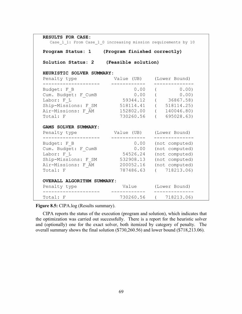
RESULTS FOR CASE: Case_1_1: From Case_1_0 increasing mission requirements by 10 Program Status: 1 (Program finished correctly) Solution Status: 2 (Feasible solution) HEURISTIC SOLVER SUMMARY: Penalty type Value (UB) (Lower Bound) -------------------- ------------ -------------- Budget: F_B 0.00 ( 0.00) Cum. Budget: F_CumB 0.00 ( 0.00) Labor: F_L 59344.12 ( 36867.58) Ship-Missions: F_SM 518114.41 ( 518114.25) Air-Missions: F_AM 152802.00 ( 140046.80) Total: F 730260.56 ( 695028.63) GAMS SOLVER SUMMARY: Penalty type Value (UB) (Lower Bound) -------------------- ------------ -------------- Budget: F_B 0.00 (not computed) Cum. Budget: F_CumB 0.00 (not computed) Labor: F_L 54526.24 (not computed) Ship-Missions: F_SM 532908.13 (not computed) Air-Missions: F_AM 200052.16 (not computed) Total: F 787486.63 ( 718213.06) OVERALL ALGORITHM SUMMARY: Penalty type Value (Lower Bound) -------------------- ------------ -------------- Total: F 730260.56 ( 718213.06)
Figure 8.5: CIPA.log (Results summary).
CIPA reports the status of the execution (program and solution), which indicates that the optimization was carried out successfully. There is a report for the heuristic solver and (optionally) one for the exact solver, both itemized by category of penalty. The overall summary shows the final solution ($730,260.56) and lower bound ($718,213.06).
69
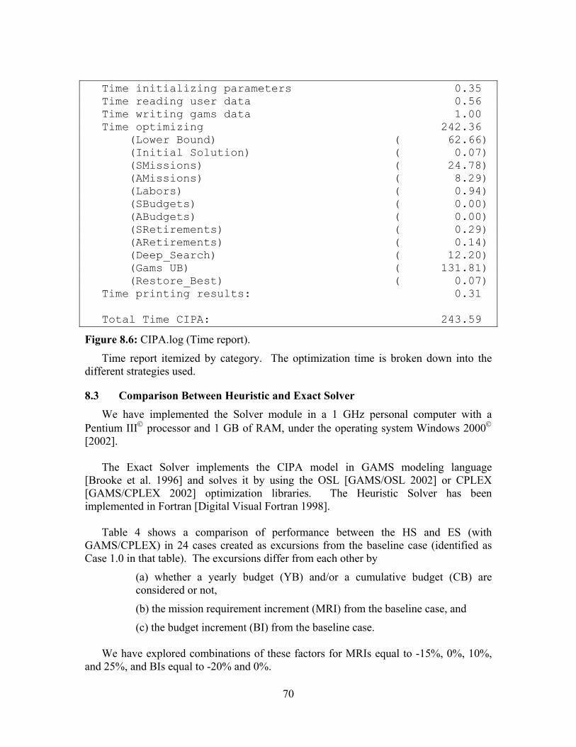
Time initializing parameters 0.35 Time reading user data 0.56 Time writing gams data 1.00 Time optimizing 242.36 (Lower Bound) ( 62.66) (Initial Solution) ( 0.07) (SMissions) ( 24.78) (AMissions) ( 8.29) (Labors) ( 0.94) (SBudgets) ( 0.00) (ABudgets) ( 0.00) (SRetirements) ( 0.29) (ARetirements) ( 0.14) (Deep_Search) ( 12.20) (Gams UB) ( 131.81) (Restore_Best) ( 0.07) Time printing results: 0.31 Total Time CIPA: 243.59
Figure 8.6: CIPA.log (Time report).
Time report itemized by category. The optimization time is broken down into the different strategies used.
8.3 Comparison Between Heuristic and Exact Solver We have implemented the Solver module in a 1 GHz personal computer with a
Pentium III processor and 1 GB of RAM, under the operating system Windows 2000 [2002].
The Exact Solver implements the CIPA model in GAMS modeling language
[Brooke et al. 1996] and solves it by using the OSL [GAMS/OSL 2002] or CPLEX [GAMS/CPLEX 2002] optimization libraries. The Heuristic Solver has been implemented in Fortran [Digital Visual Fortran 1998].
Table 4 shows a comparison of performance between the HS and ES (with
GAMS/CPLEX) in 24 cases created as excursions from the baseline case (identified as Case 1.0 in that table). The excursions differ from each other by
(a) whether a yearly budget (YB) and/or a cumulative budget (CB) are considered or not,
(b) the mission requirement increment (MRI) from the baseline case, and
(c) the budget increment (BI) from the baseline case. We have explored combinations of these factors for MRIs equal to -15%, 0%, 10%,
and 25%, and BIs equal to -20% and 0%.
70
As expected, the LB computations are clearly superior for the exact procedure, which gives an idea of the difficulty in coming up with non-trivial lower bounds by simple examination of the data. The heuristic bound can be computed in less than a second, whereas the exact bound needs between one and two minutes using GAMS/CPLEX, and 20% more on average with GAMS/OSL.
The following two columns (headed “Exact Solution” and “Heuristic Solution,”
respectively) show the findings by the exact and heuristic methods. The exact method uses GAMS/CPLEX and the figures indicate the best solution obtained after 10 minutes of computation. This is a hard integer linear program, and no case is solved during the allotted time. About half of these cases do not even yield a feasible solution. We ran these cases for hours and some of them are essentially intractable. In contrast, the heuristic solver seems to perform reasonably. The computation time for the heuristic is about 30 seconds in each of the runs, yielding high quality per unit time.
Analyzing the results in Table 4 (as well as a lot more computational experience not
shown), we find the heuristic solver highly effective and recommend it. We also find it useful to calculate an exact lower bound to support the value and accuracy of the heuristic solution. But, we only recommend the use of the exact solver to calculate a feasible solution if either:
(a) the problem dimension is small, or
(b) the heuristic solution proves unreasonable, or
(c) the heuristic solution gap is very high after computing the exact lower bound.
In any case, given the high volatility of the ES computational time, we recommend
enforcing a maximum limit (e.g., one or two hours).
71

Heuristic Exact Exact Heuristic Gap Gap
Case YB CB MRI BI LB LB Solution Solution (Exact) (Heuristic)
1.0 X 102,245 119,577 ? 124,565 ? 4.17
1.1 X 10% 695,028 718,213 787,486 736,652 9.65 2.57
1.2 X 25% 1,732,651 1,776,227 1,885,502 1,854,386 6.15 4.40
1.3 X -15% 60,374 72,953 ? 78,225 ? 7.23
2.0 X -20% 102,245 119,577 ? 127,044 ? 6.24
2.1 X 10% -20% 695,028 734,973 837,348 867,633 13.93 18.05
2.2 X 25% -20% 1,732,651 2,053,046 2,265,498 2,246,046 10.35 9.40
2.3 X -15% -20% 60,374 72,953 128,390 76,798 75.99 5.27
3.0 X X 102,245 150,476 ? 179,071 ? 19.00
3.1 X X 10% 695,028 750,519 873,864 793,604 16.43 5.74
3.2 X X 25% 1,732,651 1,830,805 2,001,855 1,926,352 9.34 5.22
3.3 X X -15% 60,374 103,791 ? 122,791 ? 18.31
4.0 X X -20% 102,245 135,488 ? 145,124 ? 7.11
4.1 X X 10% -20% 695,028 751,643 907,631 886,261 20.75 17.91
4.2 X X 25% -20% 1,732,651 2,074,060 2,303,384 2,343,700 11.06 13.00
4.3 X X -15% -20% 60,374 88,810 ? 95,945 ? 8.03
5.0 X 102,245 150,476 ? 176,455 ? 17.26
5.1 X 10% 695,028 750,519 835,994 787,605 11.39 4.94
5.2 X 25% 1,732,651 1,830,805 1,980,475 1,922,182 8.18 4.99
5.3 X -15% 60,374 103,791 ? 119,673 ? 15.30
6.0 X -20% 102,245 135,488 ? 143,235 ? 5.72
6.1 X 10% -20% 695,028 741,907 854,843 867,600 15.22 16.94
6.2 X 25% -20% 1,732,651 1,854,925 2,022,075 2,218,208 9.01 19.58
6.3 X -15% -20% 60,374 88,810 ? 98,216 ? 10.59
Table 4. Test cases run with the CIPA ES and the CIPA HS.
Legend: YB: Yearly budget; CB: Cumulative budget; MRI: Mission requirement increment (from baseline case); BI: Budget increment (from baseline case); Heur LB: Heuristic lower bound; Exact LB: Exact lower bound calculated with GAMS/CPLEX; Exact Solution: Exact solution calculated with GAMS/CPLEX in a maximum of 10 min; Heuristic Solution: Heuristic solution; Gap (Exact): Max. relative gap (%) for the exact solution; Gap (Heuristic): Max. relative gap (%) for the heuristic solution.
72
9. CIPA Project Contributions, Deliverables, and Current Status
9.1 Contributions CIPA is being developed in the Operations Research (OR) Department at the Naval Postgraduate School (NPS), Monterey, CA. Since 1999, CIPA has been funded by the Chief of Naval Operations, Assessment Division (N81) and the Office of Naval Research. CIPA principal investigators are Distinguished Professor Gerald Brown and Associate Professor Robert Dell. Research Assistant Professors Javier Salmeron and Anton Rowe have developed and integrated the CIPA algorithmic procedures and GUI, respectively. A number of NPS OR graduate students have contributed to CIPA through the following Masters Theses: Lt. R. J. Field (U.S. Navy): “Planning Capital Investment in Navy Forces,”
December 1999. Lt. N. Baran (Turkish Navy): “Optimizing Procurement Planning of Navy Ships and
Aircraft,” December 2000. LCDR R. M. Garcia (U.S. Navy): “Optimized Procurement and Retirement Planning of
Navy Ships and Aircraft,” December 2001.
9.2 Deliverables
Official versions of CIPA are those that have been delivered to N81 as testing prototypes or final versions. Versions are coded as follows: x.yy.zz where: x: p indicates prototype version, d indicates developing version, and w indicates
working version yy: consists of two numbers indicating the interface version zz: consists of two numbers indicating the heuristic solver version
73

Table 9.1 shows those versions that have been delivered as of May 1, 2002.
Version Date
Delivered Solver GUI
P.01.01 02/28/01 Only heuristic algorithm. Not scalable. Field's data preloaded. No documentation.
P.03.03 06/04/01 Only heuristic algorithm. Not scalable. Field's data preloaded. No documentation.
P.07.04 11/13/01 Only heuristic algorithm. Not scalable. Field's data preloaded. GUI tour [CIPA Quick Tour, 2001]. Basic GUI user’s guide [CIPA: User’s
manual, 2001] (unfinished). P.08.05 Internal use
only Only heuristic algorithm.
Effectiveness not included (see Appendix B)
Not scalable. Effectiveness data is not included. Instead, a
one-to-one mapping is assumed: platforms rated 0, 1 or 2 do not accomplish the mission at all, platforms rated 3, 4 or 5 do accomplish the mission entirely.
Same documentation as P.07.04. V.08.27 May 2002 Only heuristic algorithm Not scalable. Effectiveness data is included.
Table 9.1. Official versions.
74
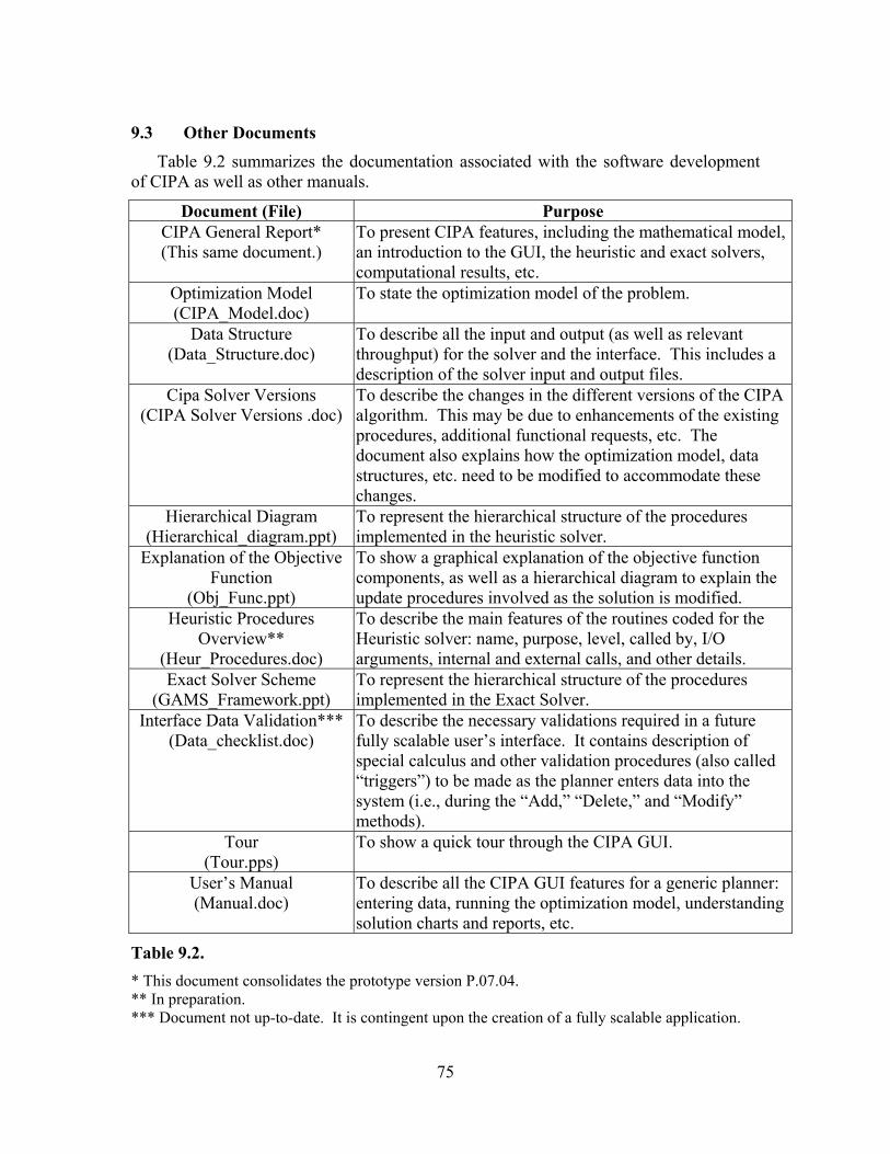
9.3 Other Documents
Table 9.2 summarizes the documentation associated with the software development of CIPA as well as other manuals.
Document (File) Purpose CIPA General Report* (This same document.)
To present CIPA features, including the mathematical model, an introduction to the GUI, the heuristic and exact solvers, computational results, etc.
Optimization Model (CIPA_Model.doc)
To state the optimization model of the problem.
Data Structure (Data_Structure.doc)
To describe all the input and output (as well as relevant throughput) for the solver and the interface. This includes a description of the solver input and output files.
Cipa Solver Versions (CIPA Solver Versions .doc)
To describe the changes in the different versions of the CIPA algorithm. This may be due to enhancements of the existing procedures, additional functional requests, etc. The document also explains how the optimization model, data structures, etc. need to be modified to accommodate these changes.
Hierarchical Diagram (Hierarchical_diagram.ppt)
To represent the hierarchical structure of the procedures implemented in the heuristic solver.
Explanation of the Objective Function
(Obj_Func.ppt)
To show a graphical explanation of the objective function components, as well as a hierarchical diagram to explain the update procedures involved as the solution is modified.
Heuristic Procedures Overview**
(Heur_Procedures.doc)
To describe the main features of the routines coded for the Heuristic solver: name, purpose, level, called by, I/O arguments, internal and external calls, and other details.
Exact Solver Scheme (GAMS_Framework.ppt)
To represent the hierarchical structure of the procedures implemented in the Exact Solver.
Interface Data Validation*** (Data_checklist.doc)
To describe the necessary validations required in a future fully scalable user’s interface. It contains description of special calculus and other validation procedures (also called “triggers”) to be made as the planner enters data into the system (i.e., during the “Add,” “Delete,” and “Modify” methods).
Tour (Tour.pps)
To show a quick tour through the CIPA GUI.
User’s Manual (Manual.doc)
To describe all the CIPA GUI features for a generic planner: entering data, running the optimization model, understanding solution charts and reports, etc.
Table 9.2. * This document consolidates the prototype version P.07.04. ** In preparation. *** Document not up-to-date. It is contingent upon the creation of a fully scalable application.
75
9.4 Current Status of the CIPA Project
As of August 1, 2002, the last version delivered to N81 is V.07.28.
In addition to consolidated versions of the CIPA system, independent research is devoted to accommodate potential user requirements. Some enhanced versions of the model and solver that have not been contemplated yet in any of the official versions are described in Appendix B of this document.
Additional research, such as aircraft age management by LCDR R. M. Garcia [2001] has not been incorporated into the existing model, algorithms, and GUI in either official or in-progress versions of CIPA.
Ongoing work by other OR NPS students is focused on improving the solution time
of the exact solver by employing integer partition schemes, as well accounting for end-effects. For the future, we consider a stochastic formulation of the model to deal with uncertain budget and mission requirements.
76
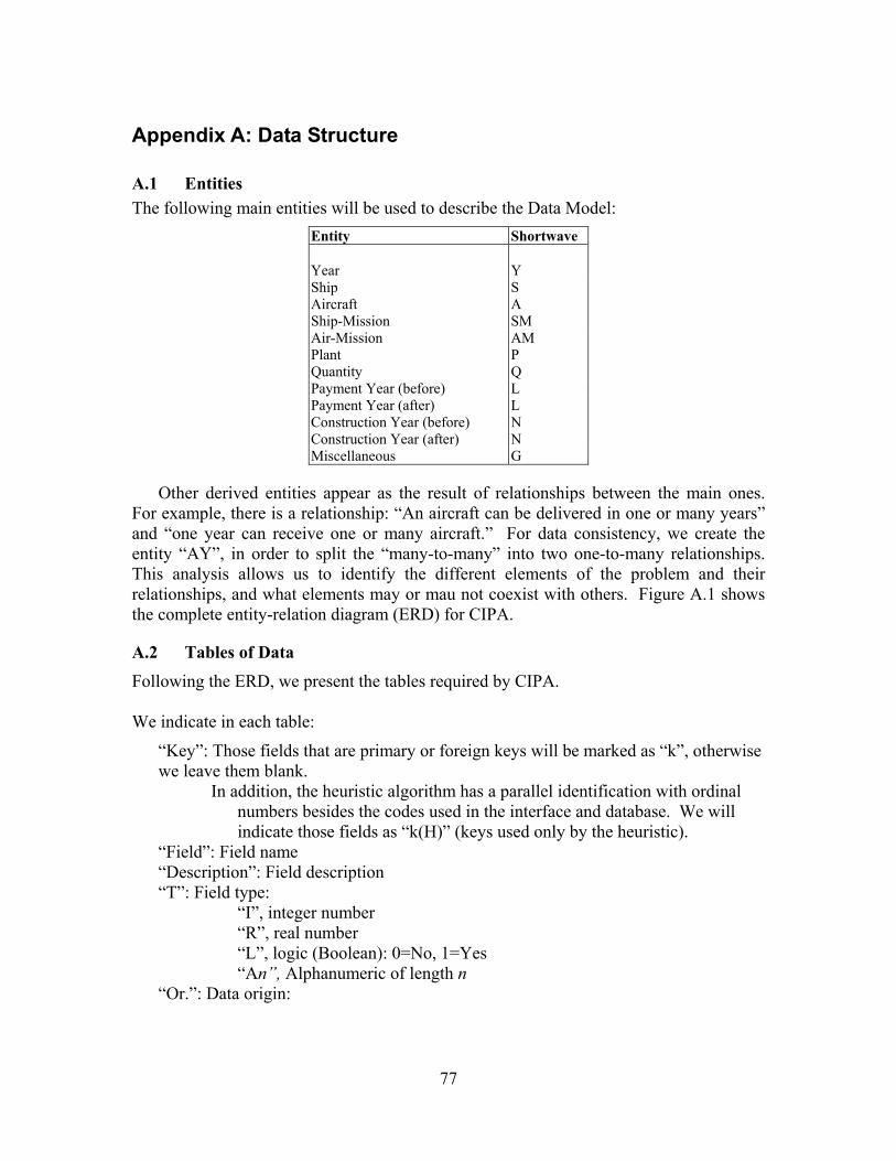
Appendix A: Data Structure
A.1 Entities The following main entities will be used to describe the Data Model:
Entity Shortwave Year Y Ship S Aircraft A Ship-Mission SM Air-Mission AM Plant P Quantity Q Payment Year (before) L Payment Year (after) L Construction Year (before) N Construction Year (after) N Miscellaneous G
Other derived entities appear as the result of relationships between the main ones. For example, there is a relationship: “An aircraft can be delivered in one or many years” and “one year can receive one or many aircraft.” For data consistency, we create the entity “AY”, in order to split the “many-to-many” into two one-to-many relationships. This analysis allows us to identify the different elements of the problem and their relationships, and what elements may or mau not coexist with others. Figure A.1 shows the complete entity-relation diagram (ERD) for CIPA.
A.2 Tables of Data Following the ERD, we present the tables required by CIPA. We indicate in each table:
“Key”: Those fields that are primary or foreign keys will be marked as “k”, otherwise we leave them blank.
In addition, the heuristic algorithm has a parallel identification with ordinal numbers besides the codes used in the interface and database. We will indicate those fields as “k(H)” (keys used only by the heuristic).
“Field”: Field name “Description”: Field description “T”: Field type:
“I”, integer number “R”, real number “L”, logic (Boolean): 0=No, 1=Yes “An”, Alphanumeric of length n
“Or.”: Data origin:
77
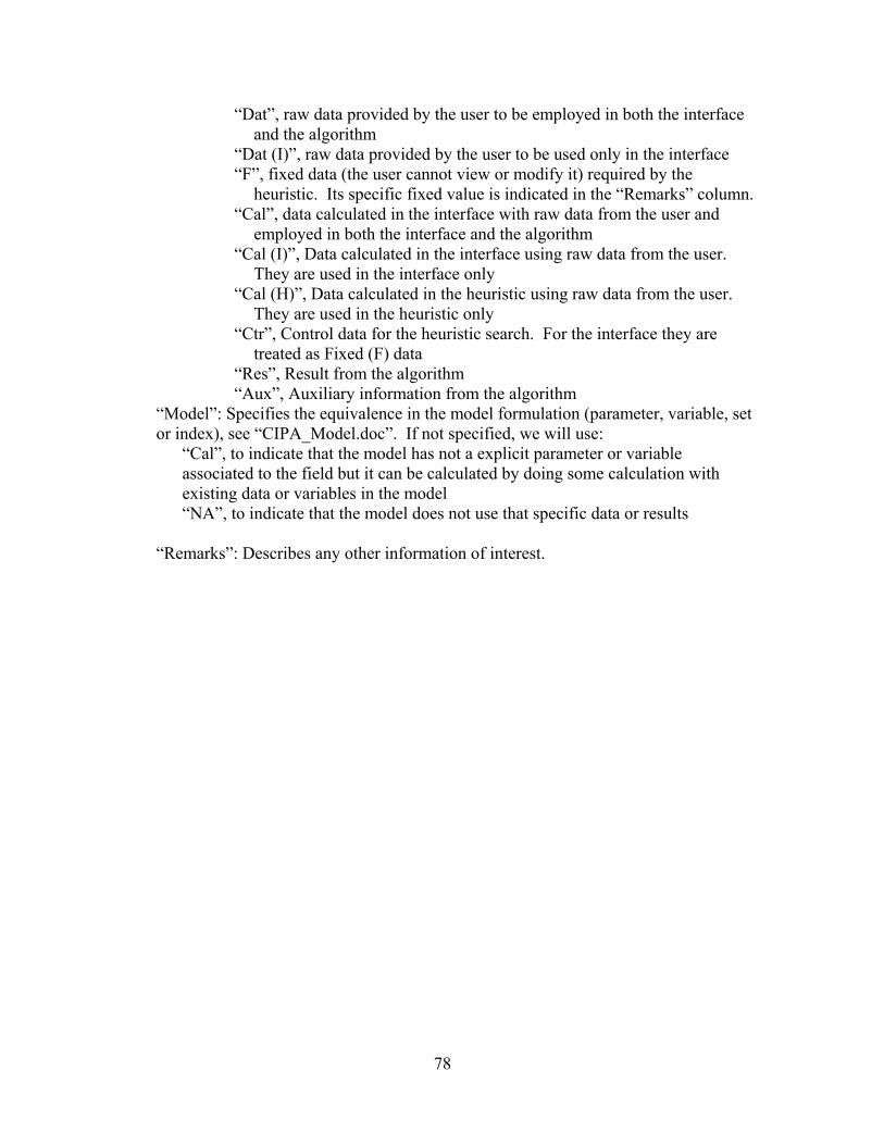
“Dat”, raw data provided by the user to be employed in both the interface and the algorithm
“Dat (I)”, raw data provided by the user to be used only in the interface “F”, fixed data (the user cannot view or modify it) required by the
heuristic. Its specific fixed value is indicated in the “Remarks” column. “Cal”, data calculated in the interface with raw data from the user and
employed in both the interface and the algorithm “Cal (I)”, Data calculated in the interface using raw data from the user.
They are used in the interface only “Cal (H)”, Data calculated in the heuristic using raw data from the user.
They are used in the heuristic only “Ctr”, Control data for the heuristic search. For the interface they are
treated as Fixed (F) data “Res”, Result from the algorithm “Aux”, Auxiliary information from the algorithm
“Model”: Specifies the equivalence in the model formulation (parameter, variable, set or index), see “CIPA_Model.doc”. If not specified, we will use:
“Cal”, to indicate that the model has not a explicit parameter or variable associated to the field but it can be calculated by doing some calculation with existing data or variables in the model “NA”, to indicate that the model does not use that specific data or results
“Remarks”: Describes any other information of interest.
78

Y S A
P
S M A M
A Y S Y
A A M
P Y
S S M A M Y S M Y
S P S P Y
C IP A : E n ti ty -R e la tio n d ia g ra m
D a s h e d l in e s re fe r to p s e u d o - re la t io n sh ip s o r p s e u d o -e n ti ty c a u se d b y th e v a lu e o f a n a tt r ib u te in a n o th e r e n tity G re y e n t i tie s g e n e ra te p r im a ry a n d fo re ig n k e y s
o n e to
m a n y
G e n e ra l (G )
A Y I I
S P L
L L l N N n
S P L l S P N S P N n
Q
S P Q L S P Q L l S P Q N S P Q N n
Figure A.1: Entity-relation diagram.
79

Table “General” Key Field Description Type Origin Model Remarks
Code of the current plan or case under analysis
A128 (NA)
Year_Ini I Dat (I) Year_End Final year of the case Dat (I) |Y|
Historical fraction of ship costs R frac apn5 R Dat 5 ISol_User L F 0 (= “No”) for the
interface Gams_Opt Use GAMS during the optimization Dat (NA)
1=Only for LB 2=Yes (LB & UB)
F_B R Res
Plan_Code Dat
1 Initial year of the case I
frac Dat apn Historical fraction of aircraft costs
Whether the user is providing an initial solution or not
(NA)
I 0=No
(Cal) Total budget penalty Update when F_B_y(y) changes
(Cal) F_CumB Total cumulative budget penalty R Res Update when F_CumB_y(y) changes
(Cal) F_L Total labor penalty R Res Update when F_L_y(y) changes
(Cal) F_SM Total Ship-Mission penalty R Res Update when F_SM_y(y) changes
(Cal) F_AM Total Air-Mission penalty R Res Update when F_AM_y(y) changes
F F Total penalty R Res Update when F_y(y) changes
(Cal) LB_F_B Lower bound on total budget penalty R Res (Cal) LB_F_CumB Lower bound on total cumulative
budget penalty R Res
(Cal) LB_F_L Lower bound on total labor penalty R Res (Cal) LB_F_SM Lower bound on total ship mission
penalty R Res
LB_F_AM Lower bound on total air mission penalty
R Res (Cal)
LB_F Lower bound on total penalty R Res (Cal) Update when LB_F_B, LB_F_CumB, LB_F_L, LB_F_SM or LB_F_AM change
CIPA_Time Total Computational time R Aux (NA) Error_Code Error Code I Aux (NA)
Error_Msg Error Message A128 Aux (NA) Error_Line Error Line in case it occurs in a data
file I Aux (NA) 0 if unavailable
Line_Header Line Header in case the error occurs in a data file
A128 Aux (NA) Blank if any
Prog_Status Program Status Code I Aux (NA) 1: Finished correctly 2: Error
Sol_Status Solution Status Code I Aux (NA) 1: Optimal 2: Feasible 3: Infeasible 4: Error optimizing 5: Error reading data 6: Error initializing
80
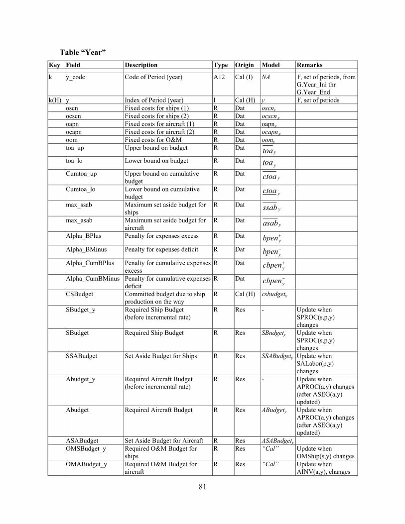
Table “Year” Key Field Description Type Origin Model Remarks
k y_code Code of Period (year) A12 Cal (I) NA Y, set of periods, from G.Year_Ini thr G.Year_End
k(H) y Index of Period (year) I Cal (H) y Y, set of periods oscn Fixed costs for ships (1) R Dat oscny ocscn Fixed costs for ships (2) R Dat ocscn,y oapn Fixed costs for aircraft (1) R Dat oapny ocapn Fixed costs for aircraft (2) R Dat ocapn,y oom Fixed costs for O&M R Dat oomy toa_up Upper bound on budget R Dat
ytoa
toa_lo Lower bound on budget R Dat ytoa
Cumtoa_up Upper bound on cumulative budget
R Dat yctoa
Cumtoa_lo Lower bound on cumulative budget
R Dat yctoa
max_ssab Maximum set aside budget for ships
R Dat yssab
max_asab Maximum set aside budget for aircraft
R Dat yasab
Alpha_BPlus Penalty for expenses excess R Dat +ybpen
Alpha_BMinus Penalty for expenses deficit R Dat −ybpen
Alpha_CumBPlus Penalty for cumulative expenses excess
R Dat +ycbpen
Alpha_CumBMinus Penalty for cumulative expenses deficit
R Dat −ycbpen
CSBudget Committed budget due to ship production on the way
R Cal (H) csbudgety
SBudget_y Required Ship Budget (before incremental rate)
R Res - Update when SPROC(s,p,y) changes
SBudget Required Ship Budget R Res SBudgety Update when SPROC(s,p,y) changes
SSABudget Set Aside Budget for Ships R Res SSABudgety Update when SALabor(p,y) changes
Abudget_y Required Aircraft Budget (before incremental rate)
R Res - Update when APROC(a,y) changes (after ASEG(a,y) updated)
Abudget Required Aircraft Budget R Res ABudgety Update when APROC(a,y) changes (after ASEG(a,y) updated)
ASABudget Set Aside Budget for Aircraft R Res ASABudgety OMSBudget_y Required O&M Budget for
ships R Res “Cal” Update when
OMShip(s,y) changes OMABudget_y Required O&M Budget for
aircraft R Res “Cal” Update when
AINV(a,y), changes
81

Key Field Description Type Origin Model Remarks OMBudget_y Required O&M Budget
(before incremental rate) R Res - Update when
OMSBudget_y(y), OMABudget_y(y) change
OMBudget Required O&M Budget R Res OMBudgety Update when OMSBudget_y(y), OMABudget_y(y) change
Budget Required Budget R Res Budgety Update when SBudget(y), ABudget(y), OMBudget(y), SSABudget(y), ASABudget(y), change
CumBudget Required Cumulative Budget R Res “Cal” Update when Budget(y) changes
F_BPlus_y Expenses excess penalty R Res “Cal” Update when Budget(y) changes
F_CumBPlus_y Cumulative expenses excess penalty
R Res “Cal” Update when CumBudget(y) changes
F_BMinus_y Expenses deficit penalty R Res “Cal” Update when Budget(y) changes
F_CumBMinus_y Cumulative expenses deficit penalty
R Res “Cal” Update when CumBudget(y) changes
F_LPlus_y Labor excess penalty R Res “Cal” Update when F_LPlus_py(p,y) changes
F_LMinus_y Labor deficit penalty R Res “Cal” Update when F_LMinus_py(p,y) changes
F_B_y Budget penalty R Res “Cal” Update when F_BPlus_y(y), F_BMinusy(y) change
F_CumB_y Cumulative budget penalty R Res “Cal” Update when F_CumBPlus_y(y), F_CumBMinusy(y) change
F_L_y Labor penalty R Res “Cal” Update when F_LPlus_y(y), F_LMinusy(y) change
F_SM_y Ship-Mission penalty R Res “Cal” Update when F_SM_smy (sm,y) changes
F_AM_y Air-Mission penalty R Res “Cal” Update when F_AM_amy (am,y) changes
F_y Total penalty in the year R Res “Cal” Update when F_B_y(y), F_L_y(y), F_SM_y(y), S_AM_y(y), change
82
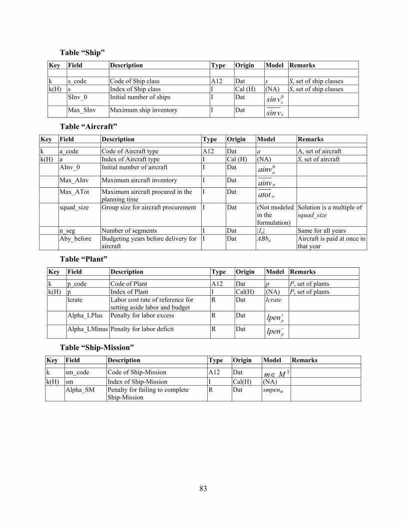
Table “Ship” Key Field Description Type Origin Model Remarks k s_code Code of Ship class A12 Dat s S, set of ship classes k(H) s Index of Ship class I Cal (H) (NA) S, set of ship classes SInv_0 Initial number of ships I Dat 0
svsin
Max_SInv Maximum ship inventory I Dat svsin
Table “Aircraft” Key Field Description Type Origin Model Remarks
k a_code Code of Aircraft type A12 Dat a A, set of aircraft k(H) a Index of Aircraft type I Cal (H) (NA) S, set of aircraft AInv_0 Initial number of aircraft I Dat 0
aainv
Max_AInv Maximum aircraft inventory I Dat aainv
Max_ATot Maximum aircraft procured in the planning time
I Dat aatot
squad_size Group size for aircraft procurement I Dat (Not modeled in the formulation)
Solution is a multiple of squad_size
n_seg Number of segments I Dat |Ia| Same for all years Aby_before Budgeting years before delivery for
aircraft I Dat ABba Aircraft is paid at once in
that year
Table “Plant” Key Field Description Type Origin Model Remarks
k p_code Code of Plant A12 Dat p P, set of plants k(H) p Index of Plant I Cal(H) (NA) P, set of plants lcrate Labor cost rate of reference for
setting aside labor and budget R Dat lcrate
Alpha_LPlus Penalty for labor excess R Dat +plpen
Alpha_LMinus Penalty for labor deficit R Dat −plpen
Table “Ship-Mission” Key Field Description Type Origin Model Remarks
k sm_code Code of Ship-Mission A12 Dat SMm ∈ k(H) sm Index of Ship-Mission I Cal(H) (NA) Alpha_SM Penalty for failing to complete
Ship-Mission R Dat smpenm
83
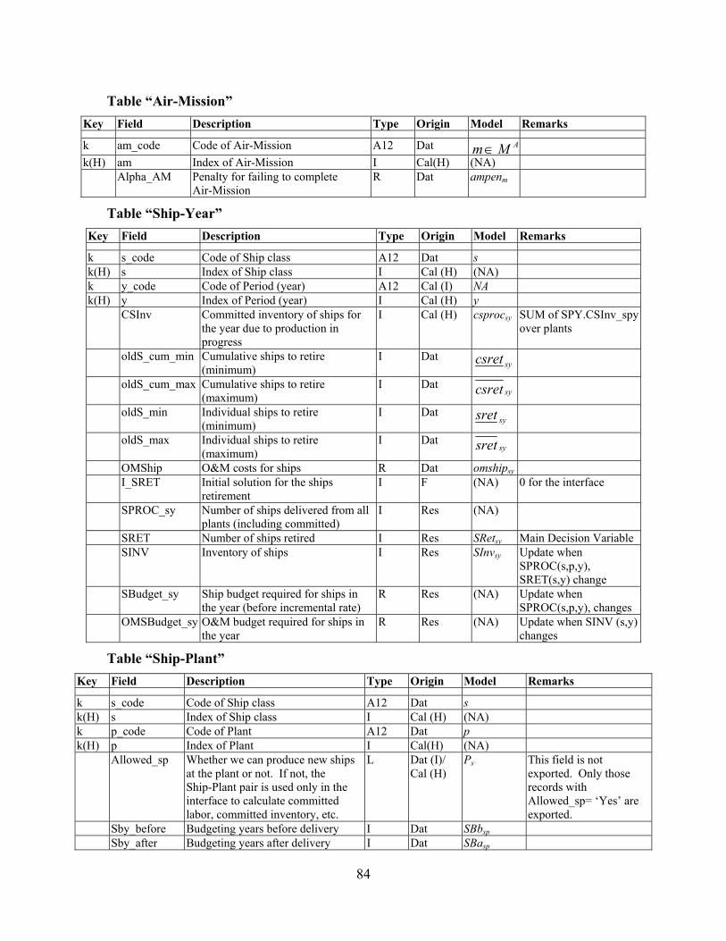
Table “Air-Mission” Key Field Description Type Origin Model Remarks
k am_code Code of Air-Mission A12 Dat AMm ∈ k(H) am Index of Air-Mission I Cal(H) (NA) Alpha_AM Penalty for failing to complete
Air-Mission R Dat ampenm
Table “Ship-Year” Key Field Description Type Origin Model Remarks
k s_code Code of Ship class A12 Dat s k(H) s Index of Ship class I Cal (H) (NA) k y_code Code of Period (year) A12 Cal (I) NA k(H) y Index of Period (year) I Cal (H) y CSInv Committed inventory of ships for
the year due to production in progress
I Cal (H) csprocsy SUM of SPY.CSInv_spy over plants
oldS_cum_min Cumulative ships to retire (minimum)
I Dat sycsret
oldS_cum_max Cumulative ships to retire (maximum)
I Dat sycsret
oldS_min Individual ships to retire (minimum)
I Dat sysret
oldS_max Individual ships to retire (maximum)
I Dat sysret
OMShip O&M costs for ships R Dat omshipsy I_SRET Initial solution for the ships
retirement I F (NA) 0 for the interface
SPROC_sy Number of ships delivered from all plants (including committed)
I Res (NA)
SRET Number of ships retired I Res SRetsy Main Decision Variable SINV Inventory of ships I Res SInvsy Update when
SPROC(s,p,y), SRET(s,y) change
SBudget_sy Ship budget required for ships in the year (before incremental rate)
R Res (NA) Update when SPROC(s,p,y), changes
OMSBudget_sy O&M budget required for ships in the year
R Res (NA) Update when SINV (s,y) changes
Table “Ship-Plant” Key Field Description Type Origin Model Remarks
k s_code Code of Ship class A12 Dat s k(H) s Index of Ship class I Cal (H) (NA) k p_code Code of Plant A12 Dat p k(H) p Index of Plant I Cal(H) (NA) Allowed_sp Whether we can produce new ships
at the plant or not. If not, the Ship-Plant pair is used only in the interface to calculate committed labor, committed inventory, etc.
L Dat (I)/ Cal (H)
Ps This field is not exported. Only those records with Allowed_sp= ‘Yes’ are exported.
Sby_before Budgeting years before delivery I Dat SBbsp Sby_after Budgeting years after delivery I Dat SBasp
84
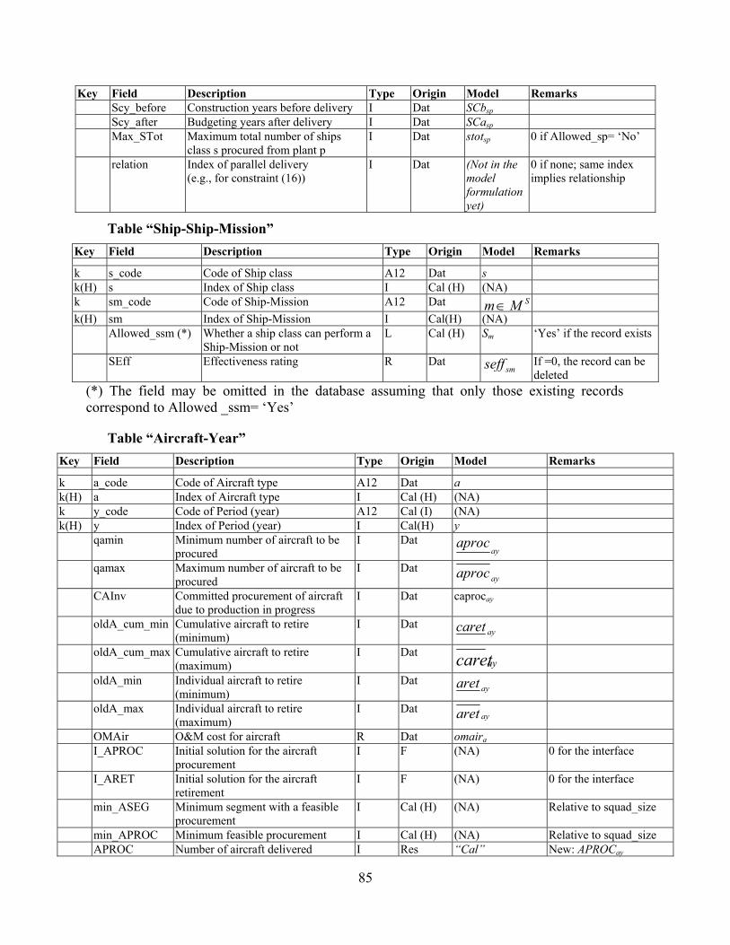
Key Field Description Type Origin Model Remarks Scy_before Construction years before delivery I Dat SCbsp Scy_after Budgeting years after delivery I Dat SCasp Max_STot Maximum total number of ships
class s procured from plant p I Dat stotsp 0 if Allowed_sp= ‘No’
relation Index of parallel delivery (e.g., for constraint (16))
I Dat (Not in the model formulation yet)
0 if none; same index implies relationship
Table “Ship-Ship-Mission” Key Field Description Type Origin Model Remarks
k s_code Code of Ship class A12 Dat s k(H) s Index of Ship class I Cal (H) (NA) k sm_code Code of Ship-Mission A12 Dat SMm ∈ k(H) sm Index of Ship-Mission I Cal(H) (NA) Allowed_ssm (*) Whether a ship class can perform a
Ship-Mission or not L Cal (H) Sm ‘Yes’ if the record exists
SEff Effectiveness rating R Dat smseff If =0, the record can be
deleted (*) The field may be omitted in the database assuming that only those existing records correspond to Allowed _ssm= ‘Yes’
Table “Aircraft-Year” Key Field Description Type Origin Model Remarks
k a_code Code of Aircraft type A12 Dat a k(H) a Index of Aircraft type I Cal (H) (NA) k y_code Code of Period (year) A12 Cal (I) (NA) k(H) y Index of Period (year) I Cal(H) y qamin Minimum number of aircraft to be
procured I Dat
ayaproc
qamax Maximum number of aircraft to be procured
I Dat ayaproc
CAInv Committed procurement of aircraft due to production in progress
I Dat caprocay
oldA_cum_min Cumulative aircraft to retire (minimum)
I Dat aycaret
oldA_cum_max Cumulative aircraft to retire (maximum)
I Dat aycaret
oldA_min Individual aircraft to retire (minimum)
I Dat ayaret
oldA_max Individual aircraft to retire (maximum)
I Dat ayaret
OMAir O&M cost for aircraft R Dat omaira I_APROC Initial solution for the aircraft
procurement I F (NA) 0 for the interface
I_ARET Initial solution for the aircraft retirement
I F (NA) 0 for the interface
min_ASEG Minimum segment with a feasible procurement
I Cal (H) (NA) Relative to squad_size
min_APROC Minimum feasible procurement I Cal (H) (NA) Relative to squad_size APROC Number of aircraft delivered I Res “Cal” New: APROCay
85

Key Field Description Type Origin Model Remarks ( ∑
∈ aIiayiocPrA ) Main Decision Variable
APROC Number of aircraft delivered (including committed)
I Res (NA)
ARET Number of aircraft retired I Res ARetay Main Decision Variable AINV Inventory of aircraft I Res AInvay Update when
APROC(a,y), ARET(a,y) change
ABudget_ay Air budget required for aircraft in the year (before incremental rate)
R Res (NA) Update when APROC(a,y), changes
Table “Aircraft-Air-Mission” Key Field Description Type Origin Model Remarks
k a_code Code of Aircraft type A12 Dat a a ∈ am k(H) a Index of Aircraft type I Cal (H) (NA) a ∈ am k am_code Code of Air-Mission A12 Dat AMm ∈ k(H) am Index of Air-Mission I Cal(H) (NA) Allowed_aam (*) Whether an aircraft type can perform
an Air-Mission or not L Cal (H) Am ‘Yes’if the record exists
AEff Effectiveness rating R Dat amaeff If =0, the record can be
deleted (*) The field may be omitted in the database assuming that only those existing records correspond to Allowed_aam = ‘Yes’
Table “Plant-Year” Key Field Description Type Origin Model Remarks
k p_code Code of Plant A12 Dat p k(H) p Index of Plant I Cal(H) (NA) k y_code Code of Period (year) A12 Cal (I) (NA) k(H) y Index of Period (year) I Cal (H) y max_sal Maximum labor set aside I Dat
pysal
CLabor Committed labor due to production in progress
I Cal (H) claborpy Relative to CSInv
pcap_up Maximum labor I Dat pypcap
pcap_lo Minimum labor I Dat py
pcap
SALabor Labor set aside I Res SALaborpy Determines SSABy LABOR Required Labor I Res Laborpy Update when
SPROC(s,p,y), SALabor(y) changes
F_LPlus_py Penalty for labor excess R Res “Cal” Update when LABOR(p,y) changes
F_LMinus_py Penalty for labor deficit R Res “Cal” Update when LABOR(p,y) changes
F_L_py Labor penalty R Res “Cal” Update when F_LPlus_py(p,y), F_LMinus_py(p,y) change (NOT needed later, though)
86
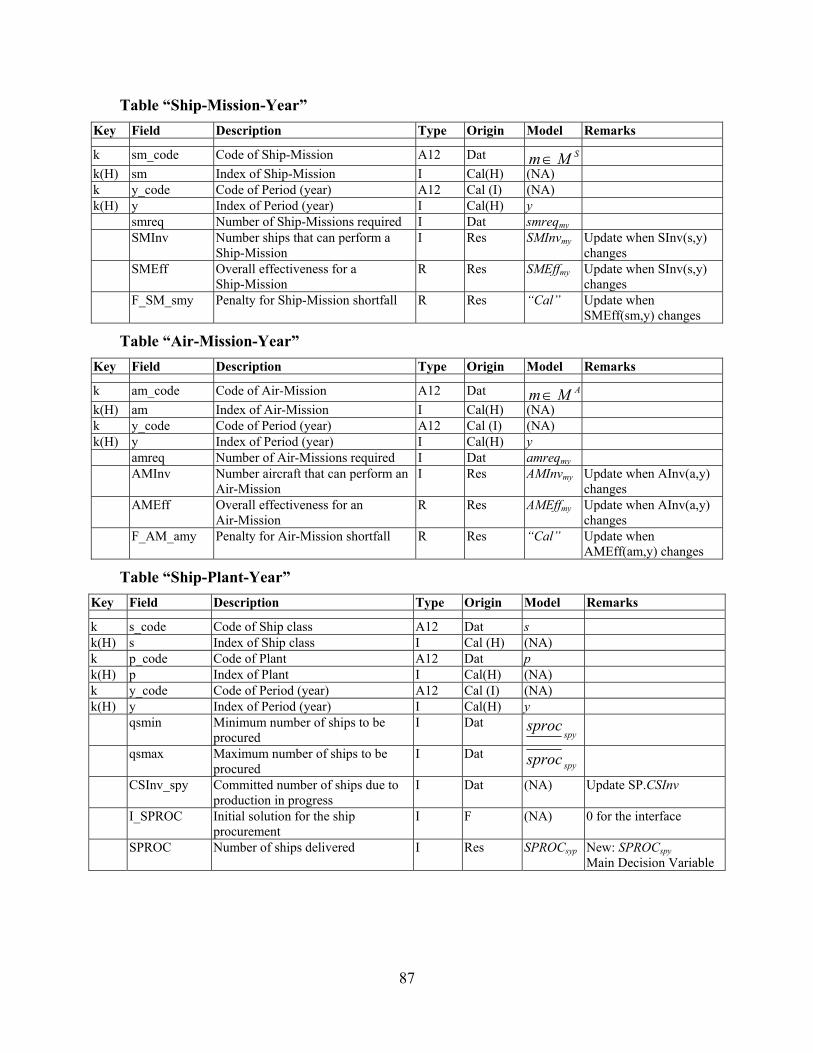
Table “Ship-Mission-Year” Key Field Description Type Origin Model Remarks
k sm_code Code of Ship-Mission A12 Dat SMm ∈ k(H) sm Index of Ship-Mission I Cal(H) (NA) k y_code Code of Period (year) A12 Cal (I) (NA) k(H) y Index of Period (year) I Cal(H) y smreq Number of Ship-Missions required I Dat smreqmy SMInv Number ships that can perform a
Ship-Mission I Res SMInvmy Update when SInv(s,y)
changes SMEff Overall effectiveness for a
Ship-Mission R Res SMEffmy Update when SInv(s,y)
changes F_SM_smy Penalty for Ship-Mission shortfall R Res “Cal” Update when
SMEff(sm,y) changes
Table “Air-Mission-Year” Key Field Description Type Origin Model Remarks
k am_code Code of Air-Mission A12 Dat AMm ∈ k(H) am Index of Air-Mission I Cal(H) (NA) k y_code Code of Period (year) A12 Cal (I) (NA) k(H) y Index of Period (year) I Cal(H) y amreq Number of Air-Missions required I Dat amreqmy AMInv Number aircraft that can perform an
Air-Mission I Res AMInvmy Update when AInv(a,y)
changes AMEff Overall effectiveness for an
Air-Mission R Res AMEffmy Update when AInv(a,y)
changes F_AM_amy Penalty for Air-Mission shortfall R Res “Cal” Update when
AMEff(am,y) changes
Table “Ship-Plant-Year” Key Field Description Type Origin Model Remarks
k s_code Code of Ship class A12 Dat s k(H) s Index of Ship class I Cal (H) (NA) k p_code Code of Plant A12 Dat p k(H) p Index of Plant I Cal(H) (NA) k y_code Code of Period (year) A12 Cal (I) (NA) k(H) y Index of Period (year) I Cal(H) y qsmin Minimum number of ships to be
procured I Dat
spysproc
qsmax Maximum number of ships to be procured
I Dat spysproc
CSInv_spy Committed number of ships due to production in progress
I Dat (NA) Update SP.CSInv
I_SPROC Initial solution for the ship procurement
I F (NA) 0 for the interface
SPROC Number of ships delivered I Res SPROCsyp New: SPROCspy Main Decision Variable
87

Table “Aircraft-Year-Segment” Key Field Description Type Origin Model Remarks
k a_code Code of Aircraft type A12 Dat a k(H) a Index of Aircraft type I Cal (H) (NA) k y_code Code of Period (year) A12 Cal (I) (NA) k(H) y Index of Period (year) I Cal(H) y k i Index of segment I Cal (I)
aIi ∈ i=1…n_seg in ‘Aircraft’
inc_lo Minimum number of aircraft in the segment
I Dat ayiinc
inc_up Maximum number of aircraft in the segment
I Dat ayiinc
aacost Lineal cost in the segment R Dat aacostayi abcost Independent term of cost in the
segment R Dat abcostayi
ASEG Whether the purchase is in the segment or not
L Res APayi Update when APROC(a,y) changes
Table “Ship-Plant-Quantity-Budgeting Year Before” Key Field Description Type Origin Model Remarks
k s_code Code of Ship class A12 Dat s Only ships that can be produced
k(H) s Index of Ship class I Cal (H) (NA) k p_code Code of Plant A12 Dat p Only plants that may
produce the ship k(H) p Index of Plant I Cal(H) (NA) k q Index of Number Ships I Cal (I) q For q=1…qmax in ‘Ship’k l Index of budgeting year (before
delivery), i.e., n=0 means delivery year, n=1 year before, …
I Cal (I) l For l=0...Sby_before-1 in ‘Ship-Plant’ (*)
scost_before Ship cost (installment) R Dat scostbspql (*) In the heuristic array structures the indices l=0, ...,Sby_before are stored as l=1,...,Sby_before+1, respectively
Table “Ship-Plant-Quantity-Budgeting Year After” Key Field Description Type Origin Model Remarks
k s_code Code of Ship class A12 Dat s Only ships that can be produced
k(H) s Index of Ship class I Cal (H) (NA) k p_code Code of Plant A12 Dat p Only plants that may
produce the ship k(H) p Index of Plant I Cal (H) (NA) k q Index of Number Ships I Cal (I) q For q=1…qmax in ‘Ship’k ll Index of budgeting year
(after delivery), i.e., n=0 means delivery year, n=1 year before, …
I Cal (I) l For ll=1...Sby_after in ‘Ship-Plant’
scost_after Ship cost (installment) R Dat scostaspql
88
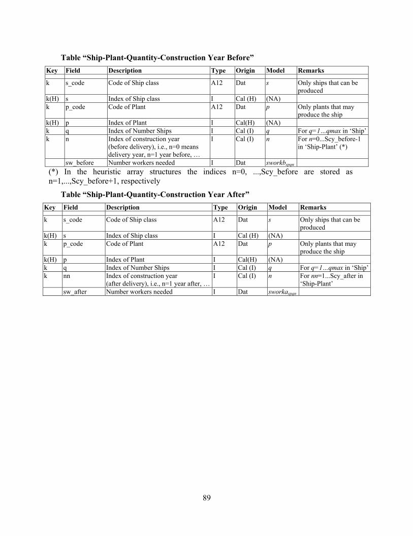
Table “Ship-Plant-Quantity-Construction Year Before” Key Field Description Type Origin Model Remarks
k s_code Code of Ship class A12 Dat s Only ships that can be produced
k(H) s Index of Ship class I Cal (H) (NA) k p_code Code of Plant A12 Dat p Only plants that may
produce the ship k(H) p Index of Plant I Cal(H) (NA) k q Index of Number Ships I Cal (I) q For q=1…qmax in ‘Ship’k n Index of construction year
(before delivery), i.e., n=0 means delivery year, n=1 year before, …
I Cal (I) n For n=0...Scy_before-1 in ‘Ship-Plant’ (*)
sw_before Number workers needed I Dat sworkbspqn (*) In the heuristic array structures the indices n=0, ...,Scy_before are stored as n=1,...,Scy_before+1, respectively
Table “Ship-Plant-Quantity-Construction Year After” Key Field Description Type Origin Model Remarks
k s_code Code of Ship class A12 Dat s Only ships that can be produced
k(H) s Index of Ship class I Cal (H) (NA) k p_code Code of Plant A12 Dat p Only plants that may
produce the ship k(H) p Index of Plant I Cal(H) (NA) k q Index of Number Ships I Cal (I) q For q=1…qmax in ‘Ship’k nn Index of construction year
(after delivery), i.e., n=1 year after, …I Cal (I) n For nn=1...Scy_after in
‘Ship-Plant’ sw_after Number workers needed I Dat sworkaspqn
89

Table “Control” Key Field Description Type Origin Model Remarks
MR_wF_SM Weight for F_SM in Mission Rank formula
R Ctr
MR_wF_AM Weight for F_AM in Mission Rank formula
R Ctr
SMR_wF_SM Weight for F_SM in Ship-Mission Rank formula
R Ctr
SMR_wF_L Weight for F_L in Ship-Mission Rank formula
R Ctr
SMR_wF_B Weight for F_B in Ship-Mission Rank formula
R Ctr
SMR_IF_F_Impr Request for Improvement in F to accept a candidate in Ship-Mission Rank
L Ctr
SMR_IF_F_SM_Impr Request for Improvement in F_SM to accept a candidate in Ship-Mission Rank
L Ctr
AMR_wF_AM Weight for F_AM in Air-Mission Rank formula
R Ctr
AMR_wF_B Weight for F_B in Air-Mission Rank formula
R Ctr
AMR_IF_F_Impr Request for Improvement in F to accept a candidate in Air-Mission Rank
L Ctr
AMR_IF_F_AM_Impr Request for Improvement in F_AM to accept a candidate in Air-Mission Rank
L Ctr
LR_wF_SM Weight for F_SM in Labor Rank formula
R Ctr
LR_wF_L Weight for F_L in Labor Rank formula R Ctr LR_wF_B Weight for F_B in Labor Rank formula R Ctr LR_IF_F_Impr Request for Improvement in F to accept
a candidate in Labor Rank L Ctr
LR_IF_F_L_Impr Request for Improvement in F_L to accept a candidate in Labor Rank
L Ctr
SRR_wIncF_SM Weight for ∆F_SM in Ship Retirement Rank formula
R Ctr
SRR_wIncOMS Weight for ∆OM Ships in Ship Retirement Rank formula
R Ctr
SRR_Max_Diff Maximum difference between ∆F_SM and ∆OM Ships to consider a candidate in Ship Retirement Rank formula
R Ctr
ARR_wIncF_AM Weight for ∆F_AM in Aircraft Retirement Rank formula
R Ctr
ARR_wIncOMA Weight for ∆OM Air in Aircraft Retirement Rank formula
R Ctr
ARR_Max_Diff Maximum difference between ∆F_AM and ∆OM Air to consider a candidate in Aircraft Retirement Rank formula
R Ctr
90
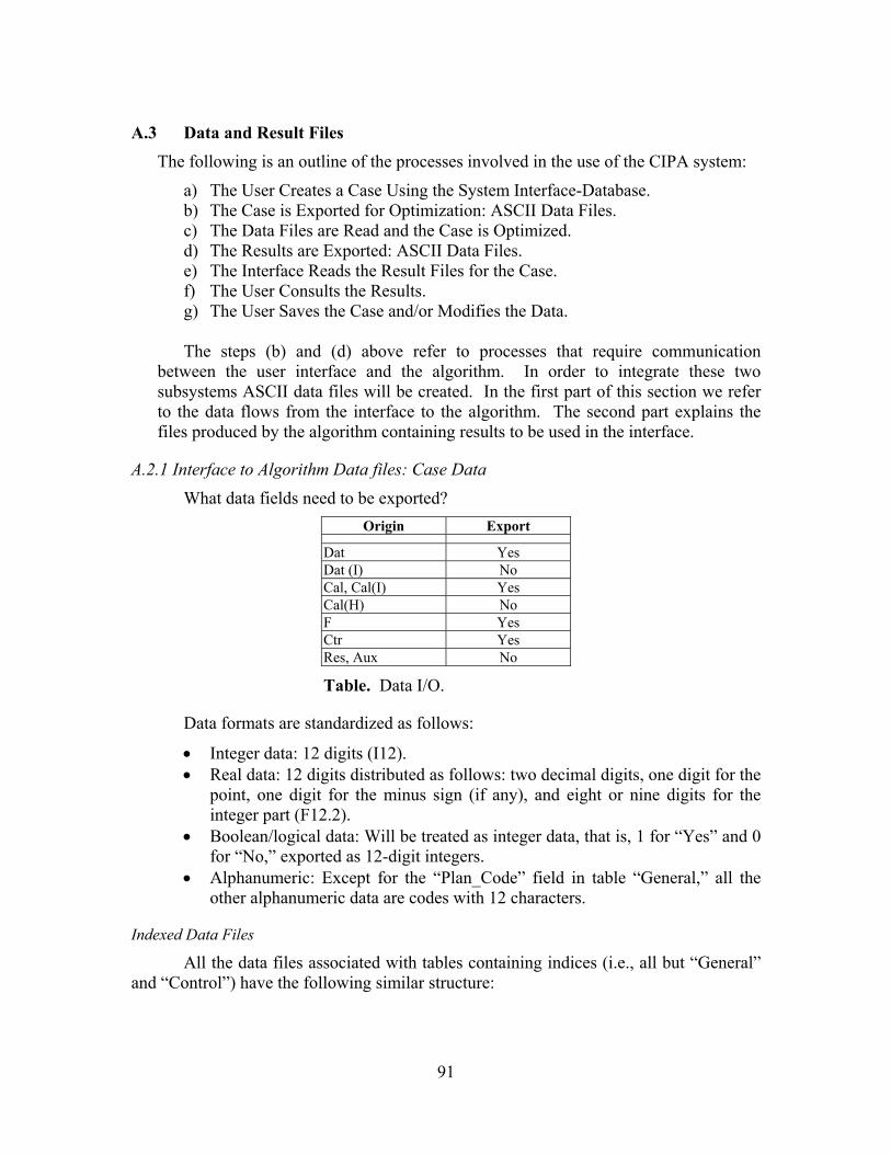
A.3 Data and Result Files
The following is an outline of the processes involved in the use of the CIPA system:
a) The User Creates a Case Using the System Interface-Database. b) The Case is Exported for Optimization: ASCII Data Files. c) The Data Files are Read and the Case is Optimized. d) The Results are Exported: ASCII Data Files. e) The Interface Reads the Result Files for the Case. f) The User Consults the Results. g) The User Saves the Case and/or Modifies the Data.
The steps (b) and (d) above refer to processes that require communication
between the user interface and the algorithm. In order to integrate these two subsystems ASCII data files will be created. In the first part of this section we refer to the data flows from the interface to the algorithm. The second part explains the files produced by the algorithm containing results to be used in the interface.
A.2.1 Interface to Algorithm Data files: Case Data
What data fields need to be exported? Origin Export
Dat Yes Dat (I) No Cal, Cal(I) Yes Cal(H) No F Yes Ctr Yes Res, Aux No
Table. Data I/O.
Data formats are standardized as follows:
• Integer data: 12 digits (I12). • Real data: 12 digits distributed as follows: two decimal digits, one digit for the
point, one digit for the minus sign (if any), and eight or nine digits for the integer part (F12.2).
• Boolean/logical data: Will be treated as integer data, that is, 1 for “Yes” and 0 for “No,” exported as 12-digit integers.
• Alphanumeric: Except for the “Plan_Code” field in table “General,” all the other alphanumeric data are codes with 12 characters.
Indexed Data Files
All the data files associated with tables containing indices (i.e., all but “General” and “Control”) have the following similar structure:
91

• File names: The location of all the data files will be the < path \Data> folder. path is the location of the program CIPA.exe (heuristic algorithm). The name of the files is provided by the indices of the table grouped together with the extension “.dat” as follows:
Table Real Name File Name
Year Y.dat Ship S.dat Aircraft A.dat Plant P.dat Ship-Mission SM.dat Air mission AM.dat Ship – Year SY.dat Ship – Plant SP.dat Ship – Ship-Mission SSM.dat Aircraft – Year AY.dat Aircraft – Air-Mission AAM.dat Plant – Year PY.dat Ship-Mission – Year SMY.out Air-Mission – Year AMY.out Ship – Plant – Year SPY.dat Aircraft – Year – Segment AYI.dat Ship – Plant – Quantity – Budgeting year before SPQL.dat Ship – Plant – Quantity – Budgeting year after SPQLL.dat Ship – Plant – Quantity – Construction year before SPQN.dat Ship – Plant – Quantity – Construction year after SPQNN.dat
Table. Tables and data files.
• File structure and contents:
Line 1 is used for comments (e.g., headers with field names). It may be left blank. From line 2 to the end of the file there is one record per line. There is a
fixed format as specified below. Every field will be associated a width of 12 columns and there will be
three blank spaces between fields. Therefore:
The first field starts in column 1 and ends in column 12. The second field starts in column 16 and ends in column 27. The third field starts in column 31 and ends in column 42. And so forth (46-57, 61-72, 76-87, ...).
92

Examples: File Y.dat y_code oscn ocscn oapn ocapn oom ... FY06 0.00 532.71 0.00 4356.30 4839.92 FY07 35.00 634.11 0.00 4874.09 4774.40 FY08 0.00 282.25 0.00 5323.42 4765.31 FY09 35.00 516.20 0.00 4721.60 4661.75 FY10 0.00 1660.92 0.00 5509.91 4669.37 FY11 35.00 391.85 0.00 6101.37 4537.59 ...
The fields are Y.y_code, Y.oscn, Y.ocscn, Y.oapn, Y.ocapn, Y.oom, Y.toa_up, Y.toa_lo, Y.Cumtoa_up, Y.Cumtoa_lo, Y.max_ssab, Y.max_asab, Y.Alpha_BPlus, Y.Alpha_BMinus, Y.Alpha_CumBPlus, Y.Alpha_CumBMinus File S.dat s_code SInv_0 Max_SInv DDG 46 999999999 DD21 0 999999999 CVX 0 999999999 SSN774 2 999999999 LHX 0 999999999 FFG 24 999999999 DD 19 999999999 CG 27 999999999 SSN688 45 999999999 SSN21 3 999999999 CVN68 9 999999999
The fields are S.s_code, S.SInv_0, S.Max_SInv File A.dat a_code AInv_0 Max_AInv Max_ATot squad_size n_seg ... JSFN 0 999999999 999999999 12 4 F18EF 218 999999999 999999999 4 4 F18AB 184 999999999 999999999 4 4 F18CD 467 999999999 999999999 4 4 F14 74 999999999 999999999 4 4
The fields are A.a_code, A.AInv_0, A.Max_AInv, A.Max_ATot, A.squad_size, A.n_seg, A.Aby_before File P.dat p_code lcrate Alpha_LPlus Alpha_LMinus Bath 0.58 0.45 0.60 Ingals 0.60 0.22 0.29 News 0.60 0.45 0.61 Eboat 0.30 0.48 0.64 Avon 0.10 0.41 0.55
The fields are P.p_code, P.lcrate, P.Alpha_LPlus, P.Alpha_LMinus
93
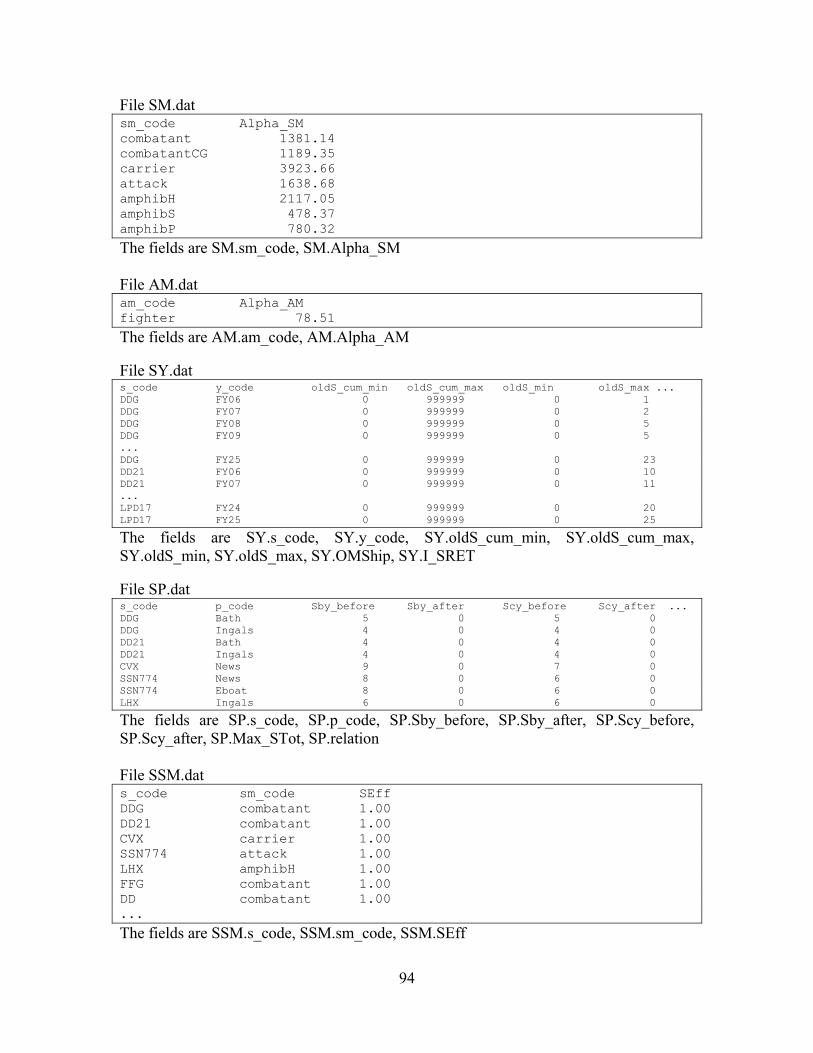
File SM.dat sm_code Alpha_SM combatant 1381.14 combatantCG 1189.35 carrier 3923.66 attack 1638.68 amphibH 2117.05 amphibS 478.37 amphibP 780.32
The fields are SM.sm_code, SM.Alpha_SM File AM.dat am_code Alpha_AM fighter 78.51
The fields are AM.am_code, AM.Alpha_AM File SY.dat s_code y_code oldS_cum_min oldS_cum_max oldS_min oldS_max ... DDG FY06 0 999999 0 1 DDG FY07 0 999999 0 2 DDG FY08 0 999999 0 5 DDG FY09 0 999999 0 5 ... DDG FY25 0 999999 0 23 DD21 FY06 0 999999 0 10 DD21 FY07 0 999999 0 11
LPD17 FY24 0 999999 0 20 LPD17 FY25 0 999999 0 25
The fields are SY.s_code, SY.y_code, SY.oldS_cum_min, SY.oldS_cum_max, SY.oldS_min, SY.oldS_max, SY.OMShip, SY.I_SRET File SP.dat s_code p_code Sby_before Sby_after Scy_before Scy_after ... DDG Bath 5 0 5 0 DDG Ingals 4 0 4 0 DD21 Bath 4 0 4 0 DD21 Ingals 4 0 4 0 CVX News 9 0 7 0 SSN774 News 8 0 6 0 SSN774 Eboat 8 0 6 0 LHX Ingals 6 0 6 0
File SSM.dat s_code sm_code SEff DDG combatant 1.00 DD21 combatant 1.00 CVX carrier 1.00 SSN774 attack 1.00
FFG combatant 1.00 DD combatant 1.00 ...
The fields are SSM.s_code, SSM.sm_code, SSM.SEff
...
The fields are SP.s_code, SP.p_code, SP.Sby_before, SP.Sby_after, SP.Scy_before, SP.Scy_after, SP.Max_STot, SP.relation
LHX amphibH 1.00
94

File AY.dat a_code y_code qamin qamax CAInv oldA_cum_min.. JSFN FY06 0 0 0 0 JSFN FY07 0 0 0 0 JSFN FY08 0 0 0 0 JSFN FY09 0 0 0 0 JSFN FY10 0 0 0 0 JSFN FY11 0 55 0 0 JSFN FY12 0 55 0 0 ... JSFN FY25 0 55 0 0 F18EF FY06 0 55 48 0 F18EF FY07 0 55 48 0 ... F14 FY25 0 0 0 74
The fields are AY.a_code, AY.y_code, AY.qamin, AY.qamax, AY.CAInv, AY.oldA_cum_min, AY.oldA_cum_max, AY.oldA_min, AY.oldA_max, AY.OMAir, AY.I_APROC, AY.I_ARET File AAM.dat a_code am_code AEffect JSFN fighter 1.00 F18EF fighter 1.00 F18AB fighter 1.00 F18CD fighter 1.00 F14 fighter 1.00 The fields are AAM.a_code, AAM.am_code, AAM.AEff File PY.dat p_code y_code max_sal pcap_up pcap_lo Bath FY06 5000 9000 2800 Bath FY07 5000 9000 2800 Bath FY08 5000 9000 2800 Bath FY09 5000 9000 2800 ... Bath FY25 5000 9000 2800 Ingals FY06 5000 17000 6500 Ingals FY07 5000 17000 6500 Ingals FY08 5000 17000 6500 ...
The fields are PY.p_code, PY.y_code, PY.max_sal, PY.pcap_up, PY.pcap_lo File SMY.dat sm_code y_code smreq combatant FY06 98 combatant FY07 98 combatant FY08 98 combatant FY09 98 combatant FY10 98 ...
The fields are SMY.sm_code, SMY.y_code, SMY.smreq
95
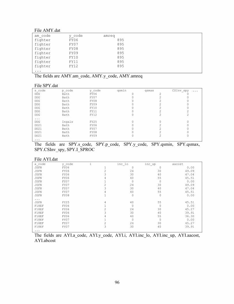
File AMY.dat am_code y_code amreq fighter FY06 895 fighter FY07 895 fighter FY08 895 fighter FY09 895 fighter FY10 895 fighter FY11 895 fighter FY12 895 ...
The fields are AMY.am_code, AMY.y_code, AMY.amreq File SPY.dat s_code p_code y_code qsmin qsmax CSInv_spy ... DDG Bath FY06 0 2 0 DDG Bath FY07 0 2 0 DDG Bath FY08 0 2 0 DDG Bath FY09 0 2 0 DDG Bath FY10 0 2 0 DDG Bath FY11 0 2 2 DDG Bath FY12 0 2 2 ... DDG Ingals FY25 0 0 0 DD21 Bath FY06 0 2 0 DD21 Bath FY07 0 2 0 DD21 Bath FY08 0 2 0 DD21 Bath FY09 0 2 0 ...
The fields are SPY.s_code, SPY.p_code, SPY.y_code, SPY.qsmin, SPY.qsmax, SPY.CSInv_spy, SPY.I_SPROC File AYI.dat a_code y_code i inc_lo inc_up aacost JSFN FY06 1 0 0 0.00 JSFN FY06 2 24 30 49.09 JSFN FY06 3 30 40 47.04 JSFN FY06 4 40 55 45.51 JSFN FY07 1 0 0 0.00 JSFN FY07 2 24 30 49.09 JSFN FY07 3 30 40 47.04 JSFN FY07 4 40 55 45.51 JSFN FY08 1 0 0 0.00 ... JSFN FY25 4 40 55 45.51 F18EF FY06 1 0 0 0.00 F18EF FY06 2 24 30 45.27 F18EF FY06 3 30 40 39.91 F18EF FY06 4 40 55 36.30 F18EF FY07 1 0 0 0.00 F18EF FY07 2 24 30 45.27 F18EF FY07 3 30 40 39.91 ...
The fields are AYI.a_code, AYI.y_code, AYI.i, AYI.inc_lo, AYI.inc_up, AYI.aacost, AYI.abcost
96
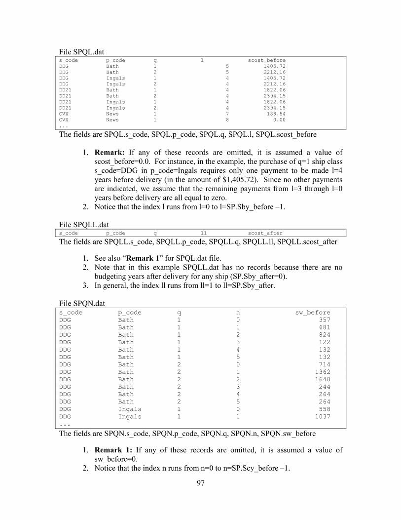
File SPQL.dat s_code p_code q l scost_before DDG Bath 1 5 1405.72 DDG Bath 2 5 2212.16 DDG Ingals 1 4 1405.72 DDG Ingals 2 4 2212.16 DD21 Bath 1 4 1822.06 DD21 Bath 2 4 2394.15 DD21 Ingals 1 4 1822.06 DD21 Ingals 2 4 2394.15 CVX News 1 7 188.54 CVX News 1 8 0.00 ...
The fields are SPQL.s_code, SPQL.p_code, SPQL.q, SPQL.l, SPQL.scost_before
1. Remark: If any of these records are omitted, it is assumed a value of scost_before=0.0. For instance, in the example, the purchase of q=1 ship class s_code=DDG in p_code=Ingals requires only one payment to be made l=4 years before delivery (in the amount of $1,405.72). Since no other payments are indicated, we assume that the remaining payments from l=3 through l=0 years before delivery are all equal to zero.
2. Notice that the index l runs from l=0 to l=SP.Sby_before –1. File SPQLL.dat s_code p_code q ll scost_after
The fields are SPQLL.s_code, SPQLL.p_code, SPQLL.q, SPQLL.ll, SPQLL.scost_after
1. See also “Remark 1” for SPQL.dat file. 2. Note that in this example SPQLL.dat has no records because there are no
budgeting years after delivery for any ship (SP.Sby_after=0). 3. In general, the index ll runs from ll=1 to ll=SP.Sby_after.
File SPQN.dat s_code p_code q n sw_before DDG Bath 1 0 357 DDG Bath 1 1 681 DDG Bath 1 2 824 DDG Bath 1 3 122 DDG Bath 1 4 132 DDG Bath 1 5 132 DDG Bath 2 0 714 DDG Bath 2 1 1362 DDG Bath 2 2 1648 DDG Bath 2 3 244 DDG Bath 2 4 264 DDG Bath 2 5 264 DDG Ingals 1 0 558 DDG Ingals 1 1 1037 ...
The fields are SPQN.s_code, SPQN.p_code, SPQN.q, SPQN.n, SPQN.sw_before
1. Remark 1: If any of these records are omitted, it is assumed a value of sw_before=0.
2. Notice that the index n runs from n=0 to n=SP.Scy_before –1.
97
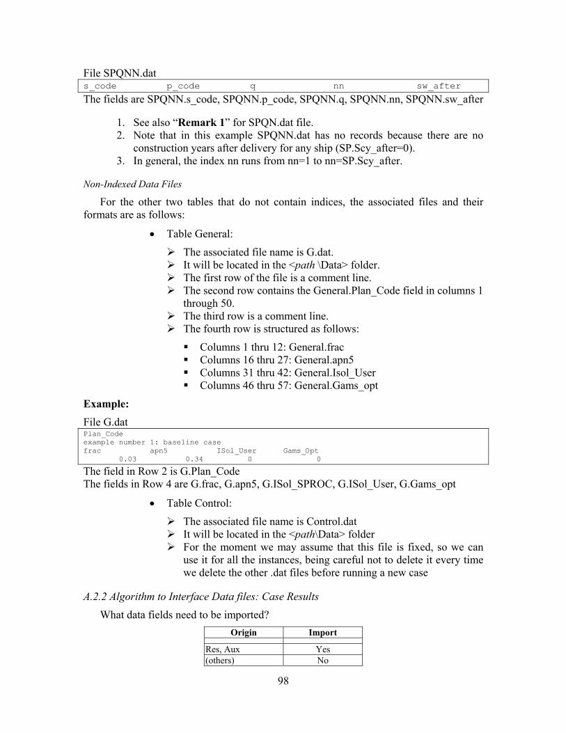
File SPQNN.dat s_code p_code q nn sw_after
The fields are SPQNN.s_code, SPQNN.p_code, SPQNN.q, SPQNN.nn, SPQNN.sw_after
1. See also “Remark 1” for SPQN.dat file. 2. Note that in this example SPQNN.dat has no records because there are no
construction years after delivery for any ship (SP.Scy_after=0). 3. In general, the index nn runs from nn=1 to nn=SP.Scy_after.
Non-Indexed Data Files
For the other two tables that do not contain indices, the associated files and their formats are as follows:
• Table General:
The associated file name is G.dat. It will be located in the <path \Data> folder. The first row of the file is a comment line. The second row contains the General.Plan_Code field in columns 1
through 50. The third row is a comment line. The fourth row is structured as follows:
Columns 1 thru 12: General.frac Columns 16 thru 27: General.apn5 Columns 31 thru 42: General.Isol_User Columns 46 thru 57: General.Gams_opt
Example: File G.dat Plan_Code example number 1: baseline case frac apn5 ISol_User Gams_Opt 0.03 0.34 0 0
The field in Row 2 is G.Plan_Code The fields in Row 4 are G.frac, G.apn5, G.ISol_SPROC, G.ISol_User, G.Gams_opt
• Table Control:
The associated file name is Control.dat It will be located in the <path\Data> folder For the moment we may assume that this file is fixed, so we can
use it for all the instances, being careful not to delete it every time we delete the other .dat files before running a new case
A.2.2 Algorithm to Interface Data files: Case Results
What data fields need to be imported? Origin Import
Res, Aux Yes (others) No
98
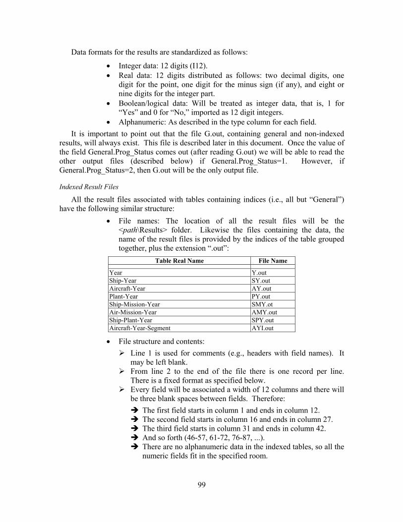
Data formats for the results are standardized as follows:
• Integer data: 12 digits (I12). • Real data: 12 digits distributed as follows: two decimal digits, one
digit for the point, one digit for the minus sign (if any), and eight or nine digits for the integer part.
• Boolean/logical data: Will be treated as integer data, that is, 1 for “Yes” and 0 for “No,” imported as 12 digit integers.
• Alphanumeric: As described in the type column for each field. It is important to point out that the file G.out, containing general and non-indexed
results, will always exist. This file is described later in this document. Once the value of the field General.Prog_Status comes out (after reading G.out) we will be able to read the other output files (described below) if General.Prog_Status=1. However, if General.Prog_Status=2, then G.out will be the only output file.
Indexed Result Files
All the result files associated with tables containing indices (i.e., all but “General”) have the following similar structure:
• File names: The location of all the result files will be the <path\Results> folder. Likewise the files containing the data, the name of the result files is provided by the indices of the table grouped together, plus the extension “.out”:
Table Real Name File Name
Year Y.out Ship-Year SY.out Aircraft-Year AY.out Plant-Year PY.out Ship-Mission-Year SMY.ot Air-Mission-Year AMY.out Ship-Plant-Year SPY.out Aircraft-Year-Segment AYI.out
• File structure and contents: Line 1 is used for comments (e.g., headers with field names). It
may be left blank. From line 2 to the end of the file there is one record per line.
There is a fixed format as specified below. Every field will be associated a width of 12 columns and there will
be three blank spaces between fields. Therefore: The first field starts in column 1 and ends in column 12. The second field starts in column 16 and ends in column 27. The third field starts in column 31 and ends in column 42. And so forth (46-57, 61-72, 76-87, ...). There are no alphanumeric data in the indexed tables, so all the numeric fields fit in the specified room.
99

Example:
File Y.out y_code SBudget_y SBudget SSABudget ABudget_y ABudget ASABudget ... FY06 12962.10 13899.65 0.00 8038.74 16591.83 0.00 FY07 9967.92 10955.09 0 00 8618.67 16735.75 0.00 FY08 10845.90 11462.00 0.00 9121.92 17284.30 0.00 FY09 8499.41 9321.08 0.00 11206.09 17427.19 0.00 ...
The fields are Y.y_code, Y.SBudget_y, Y.SBudget, Y.SSABudget, Y.ABudget_y, Y.ABudget, Y.ASABudget, Y.OMSBudget_y, Y.OMABudget_y, Y.OMBudget_y, Y.OMBudget, Y.Budget, Y.CumBudget, Y.F_BPlus_y, Y.F_CumBPlus_y, Y.F_BMinus_y, Y.F_CumBMinus_y, Y.F_LPlus_y, Y.F_LMinus_y, Y.F_B_y, Y.F_CumB_y, Y.F_L_y, Y.F_SM_y, Y.F_AM_y, Y.F_y File SY.out s_code y_code SPROC_sy SRET SINV SBudget_sy DDG FY06 3 0 49 2212.16 DDG FY07 1 0 50 0.00 DDG FY08 4 0 54 0.00 DDG FY09 1 0 55 0.00 DDG FY10 0 0 55 0.00 ...
The fields are SY.s_code, SY.y_code, SY.SPROC_sy, SY.SRET, SY.SINV
File AY.out a_code y_code APROC APROC_ay ARET AINV ... JSFN FY06 0 0 0 0 JSFN FY07 0 0 0 0 JSFN FY08 0 0 0 0 JSFN FY09 0 0 0 0 JSFN FY10 0 0 0 0 ...
The fields are AY.a_code, AY.y_code, AY.APROC, AY.APROC_ay, AY.ARET, AY.AINV, AY.ABudget_ay
File PY.out p_code y_code SALabor LABOR F_LPlus_py F_LMinus_py F_L_py Bath FY06 0.00 4209 0.00 0.00 0.00 Bath FY07 0.00 6180 0.00 0.00 0.00 Bath FY08 0.00 7292 0.00 0.00 0.00 Bath FY09 0.00 8174 0.00 0.00 0.00 Bath FY10 0.00 9292 131.40 0.00 131.40 Bath FY11 0.00 8358 0.00 0.00 0.00 ...
The fields are PY.p_code, PY.y_code, PY.SALabor, PY.LABOR, PY.F_LPlus_py, PY.F_LMinus_py, PY.F_L_py
File SMY.out sm_code y_code SMInv SMEff F_SM_smy combatant FY06 92 92.00 8286.84 combatant FY07 90 90.00 11049.12 ...
The fields are SMY.sm_code, SMY.y_code, SMY.SMInv, SMInv.SMEff, SMY.F_SM_smy
100
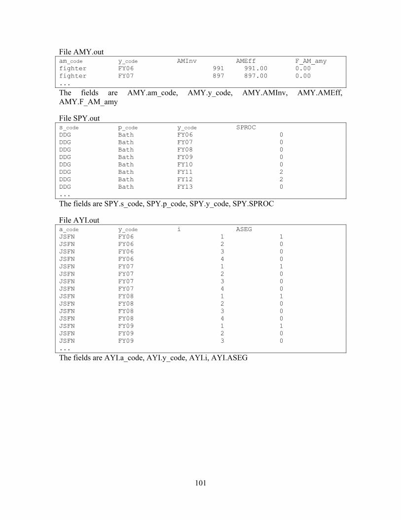
File AMY.out am_code y_code AMInv AMEff F_AM_amy fighter FY06 991 991.00 0.00 fighter FY07 897 897.00 0.00 ...
The fields are AMY.am_code, AMY.y_code, AMY.AMInv, AMY.AMEff, AMY.F_AM_amy File SPY.out s_code p_code y_code SPROC DDG Bath FY06 0 DDG Bath FY07 0 DDG Bath FY08 0 DDG Bath FY09 0 DDG Bath FY10 0 DDG Bath FY11 2 DDG Bath FY12 2 DDG Bath FY13 0 ...
The fields are SPY.s_code, SPY.p_code, SPY.y_code, SPY.SPROC File AYI.out a_code y_code i ASEG JSFN FY06 1 1 JSFN FY06 2 0 JSFN FY06 3 0 JSFN FY06 4 0 JSFN FY07 1 1 JSFN FY07 2 0 JSFN FY07 3 0 JSFN FY07 4 0 JSFN FY08 1 1 JSFN FY08 2 0 JSFN FY08 3 0 JSFN FY08 4 0 JSFN FY09 1 1 JSFN FY09 2 0 JSFN FY09 3 0 ...
The fields are AYI.a_code, AYI.y_code, AYI.i, AYI.ASEG
101

Non-Indexed Result Files
The Table “General” does not contain indices but contains results. It has the following features:
• Table General: The associated file with results is G.out It will be located in the <path\Results> folder There is a fixed format for the first seven rows of this file:
o Row 1 may be disregarded o Row 2 contains the following result fields:
Columns 1 through 12: G.Prog_Status (Integer, 12 digits)
This code means:
General.Prog_Status Value Meaning
1 Program executed without errors 2 An error occurred
Columns 16 through 27: G.Sol_Status. (Integer, 12 digits).
This code means:
General.Sol_Status Value Meaning
1 Optimal solution 2 Feasible solution 3 Problem infeasible 4 Error while optimizing 5 Error while reading data 6 Error while initializing
Columns 31 through 42: G.Error_Code (Integer, 12 digits)
(It will be set to zero if G.Prog_Status=1). Columns 46 through 57: G.Error_Line (Integer, 12 digits)
(It will be set to zero if G.Prog_Status=1). Columns 61 through 72: G.F_B (Real, 12 digits, 2 for decimal digits). (It will be set to zero if G.Prog_Status=2).
Columns 76 through 87: G.F_CumB (Real, 12 digits, 2 for decimal digits). (It will be set to zero if G.Prog_Status=2).
Columns 91 through 102: G.F_L (Real, 12 digits, 2 for decimal digits). (It will be set to zero if G.Prog_Status=2).
Columns 106 through 117: G.F_SM (Real, 12 digits, 2 for decimal digits). (It will be set to zero if G.Prog_Status=2).
Columns 121 through 132: G.F_AM (Real, 12 digits, 2 for decimal digits). (It will be set to zero if G.Prog_Status=2).
Columns 136 through 147: G.F (Real, 12 digits, 2 for decimal digits). (It will be set to zero if G.Prog_Status=2).
102
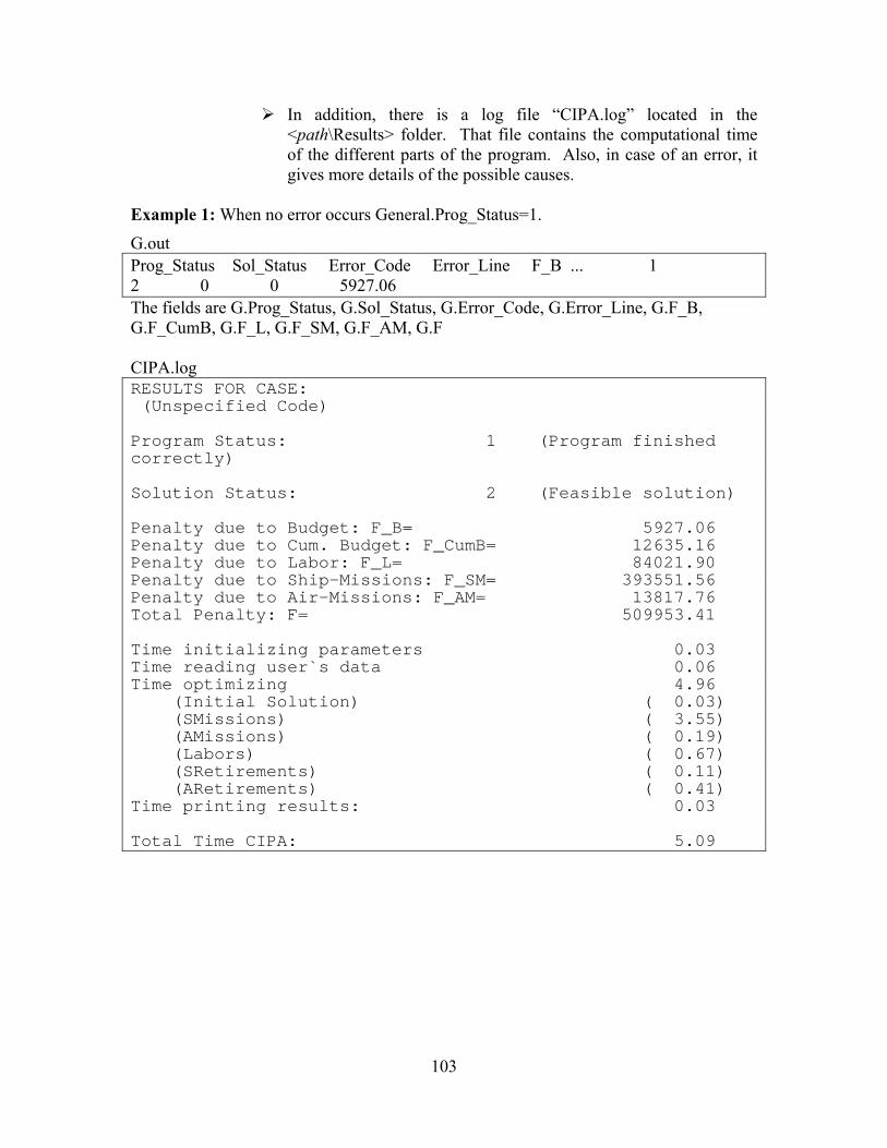
In addition, there is a log file “CIPA.log” located in the <path\Results> folder. That file contains the computational time of the different parts of the program. Also, in case of an error, it gives more details of the possible causes.
Example 1: When no error occurs General.Prog_Status=1.
G.out Prog_Status Sol_Status Error_Code Error_Line F_B ... 1 2 0 0 5927.06 The fields are G.Prog_Status, G.Sol_Status, G.Error_Code, G.Error_Line, G.F_B, G.F_CumB, G.F_L, G.F_SM, G.F_AM, G.F CIPA.log RESULTS FOR CASE: (Unspecified Code) Program Status: 1 (Program finished correctly) Solution Status: 2 (Feasible solution) Penalty due to Budget: F_B= 5927.06 Penalty due to Cum. Budget: F_CumB= 12635.16 Penalty due to Labor: F_L= 84021.90 Penalty due to Ship-Missions: F_SM= 393551.56 Penalty due to Air-Missions: F_AM= 13817.76 Total Penalty: F= 509953.41 Time initializing parameters 0.03 Time reading user`s data 0.06 Time optimizing 4.96 (Initial Solution) ( 0.03) (SMissions) ( 3.55) (AMissions) ( 0.19) (Labors) ( 0.67) (SRetirements) ( 0.11) (ARetirements) ( 0.41) Time printing results: 0.03 Total Time CIPA: 5.09
103
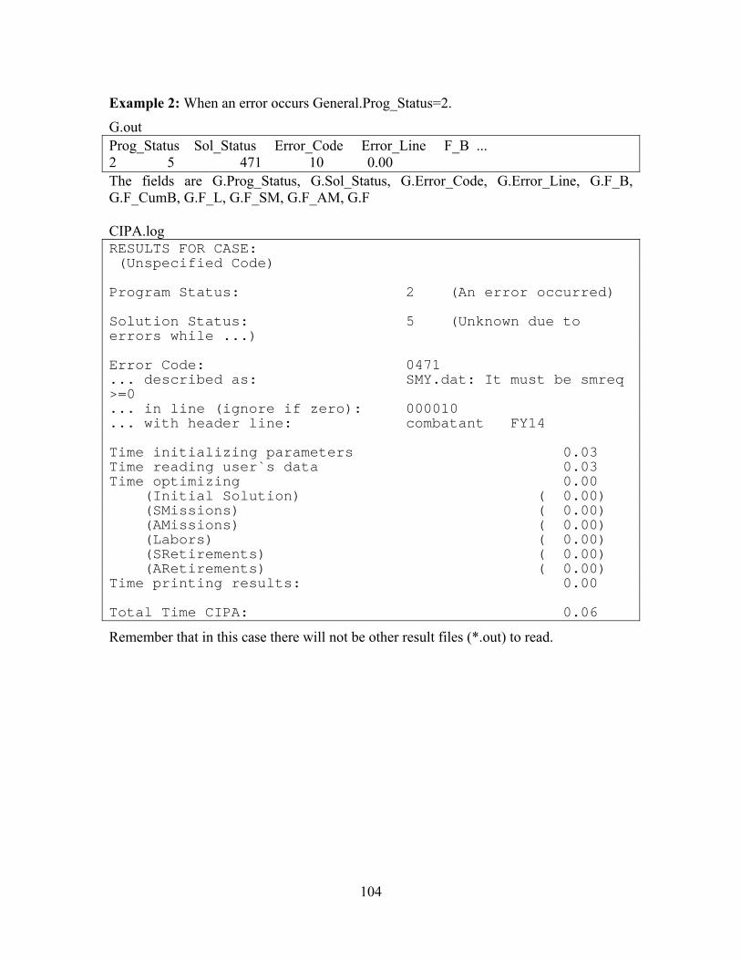
Example 2: When an error occurs General.Prog_Status=2.
G.out Prog_Status Sol_Status Error_Code Error_Line F_B ... 2 5 471 10 0.00 The fields are G.Prog_Status, G.Sol_Status, G.Error_Code, G.Error_Line, G.F_B, G.F_CumB, G.F_L, G.F_SM, G.F_AM, G.F CIPA.log RESULTS FOR CASE: (Unspecified Code) Program Status: 2 (An error occurred) Solution Status: 5 (Unknown due to errors while ...) Error Code: 0471 ... described as: SMY.dat: It must be smreq >=0 ... in line (ignore if zero): 000010 ... with header line: combatant FY14 Time initializing parameters 0.03 Time reading user`s data 0.03 Time optimizing 0.00 (Initial Solution) ( 0.00) (SMissions) ( 0.00) (AMissions) ( 0.00) (Labors) ( 0.00) (SRetirements) ( 0.00) (ARetirements) ( 0.00) Time printing results: 0.00 Total Time CIPA: 0.06
Remember that in this case there will not be other result files (*.out) to read.
104

Appendix B: New Versions of the CIPA Solver
B.1 Introduction The internal version of the Solver (that used for development purposes, not for
official deliverables) that we consider as the starting point is the so-called Ver_25. This is the version whose characteristics, model, and algorithms have been described in this report.
When a new version of the CIPA Solver is developed, many documents may need to
be updated (i.e., they will contain the information for the most updated version): CIPA General Report (this document), Optimization Model, Data Structure, Hierarchical, and Flow Diagrams, etc.
As opposed to those documents, source files (for both the heuristic and the exact
solvers), executable codes, data files, and result files will be associated with specific versions. This means that they will appear under a folder with the version name on it:
...cipa path \exe
\ver_25 (executable code “Cipa.exe” for ver_25) ... \ver_28 (executable code “Cipa.exe” for ver_28)
\data \ver_25 (contains data files for cases to be run with ver_25) ... \ver_28 (contains data files for cases to be run with ver_28)
\source \ver_25 (contains heuristic source files for version ver_25) ... \ver_28 (contains heuristic source files for version ver_28)
\gams \ver_25 (contains exact source files for version ver_25) ... \ver_28 (contains exact source files for version ver_28)
\results \ver_25 (contains result files for cases run with ver_25) ... \ver_28 (contains result files for cases run with ver_28)
105
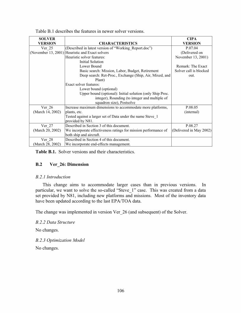
Table B.1 describes the features in newer solver versions. SOLVER VERSION CHARACTERISTICS
CIPA VERSION
Ver_25 (November 13, 2001)
(Described in latest version of “Working_Report.doc”) Heuristic and Exact solvers Heuristic solver features:
Initial Solution Lower Bound Basic search: Mission, Labor, Budget, Retirement Deep search: Ret-Proc., Exchange (Ship, Air, Mixed, and
Plant) Exact solver features:
Lower bound (optional) Upper bound (optional): Initial solution (only Ship Proc.
integer), Rounding (to integer and multiple of squadron size), Postsolve
P.07.04 (Delivered on
November 13, 2001)
Remark: The Exact Solver call is blocked
out.
Ver_26 (March 14, 2002)
Increase maximum dimensions to accommodate more platforms, plants, etc. Tested against a larger set of Data under the name Steve_1 provided by N81.
P.08.05 (internal)
Ver_27 (March 20, 2002)
Described in Section 3 of this document. We incorporate effectiveness ratings for mission performance of both ship and aircraft.
P.08.27 (Delivered in May 2002)
Ver_28 (March 28, 2002)
Described in Section 4 of this document. We incorporate end-effects management.
Table B.1. Solver versions and their characteristics.
B.2 Ver_26: Dimension
B.2.1 Introduction
This change aims to accommodate larger cases than in previous versions. In particular, we want to solve the so-called “Steve_1” case. This was created from a data set provided by N81, including new platforms and missions. Most of the inventory data have been updated according to the last EPA/TOA data. The change was implemented in version Ver_26 (and subsequent) of the Solver.
B.2.2 Data Structure
No changes.
B.2.3 Optimization Model
No changes.
106
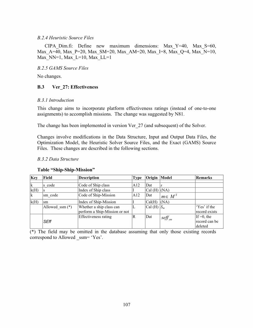
B.2.4 Heuristic Source Files
CIPA_Dim.fi: Define new maximum dimensions: Max_Y=40, Max_S=60, Max_A=40, Max_P=20, Max_SM=20, Max_AM=20, Max_I=8, Max_Q=4, Max_N=10, Max_NN=1, Max_L=10, Max_LL=1
B.2.5 GAMS Source Files
No changes.
B.3 Ver_27: Effectiveness
B.3.1 Introduction
This change aims to incorporate platform effectiveness ratings (instead of one-to-one assignments) to accomplish missions. The change was suggested by N81. The change has been implemented in version Ver_27 (and subsequent) of the Solver. Changes involve modifications in the Data Structure, Input and Output Data Files, the Optimization Model, the Heuristic Solver Source Files, and the Exact (GAMS) Source Files. These changes are described in the following sections.
B.3.2 Data Structure
Table “Ship-Ship-Mission” Key Field Description Type Origin Model Remarks
k s_code Code of Ship class A12 Dat s k(H) s Index of Ship class I Cal (H) (NA) k sm_code Code of Ship-Mission A12 Dat SMm ∈
k(H) sm Index of Ship-Mission I Cal(H) (NA) Allowed_ssm (*) Whether a ship class can
perform a Ship-Mission or not L Cal (H) Sm ‘Yes’ if the
record exists
SEff Effectiveness rating R Dat
smseff If =0, the record can be deleted
(*) The field may be omitted in the database assuming that only those existing records correspond to Allowed _ssm= ‘Yes’.
107

Table “Aircraft-Air-Mission” Key Field Description Type Origin Model Remarks
k a_code Code of Aircraft type A12 Dat a a ∈ am k(H) a Index of Aircraft type I Cal (H) (NA) a ∈ am k am_code Code of Air-Mission A12 Dat AMm ∈
k(H) am Index of Air-Mission I Cal(H) (NA) Allowed_aam (*) Whether an aircraft type can
perform an Air-Mission or not L Cal (H) Am ‘Yes’if the
record exists
AEff Effectiveness rating R Dat
amaeff If =0, the record can be deleted
(*) The field may be omitted in the database assuming that only those existing records correspond to Allowed_aam = ‘Yes’.
Table “Ship-Mission-Year” Key Field Description Type Origin Model Remarks
k sm_code Code of Ship-Mission A12 Dat SMm ∈
k(H) sm Index of Ship-Mission I Cal(H) (NA) k y_code Code of Period (year) A12 Cal (I) (NA) k(H) y Index of Period (year) I Cal(H) y smreq Number of Ship-Missions
required I Dat smreqmy
SMInv Number ships that can perform a Ship-Mission
I Res SMInvmy Update when SInv(s,y) changes
SMEff
Overall effectiveness for a Ship-Mission
R Res SMEffmy Update when SInv(s,y) changes
F_SM_smy Penalty for Ship-Mission shortfall
R Res “Cal” UPDATE WHEN SMEFF(SM,Y) CHANGES
108

Table “Air-Mission-Year” Key Field Description Type Origin Model Remarks
k am_code Code of Air-Mission A12 Dat AMm ∈
k(H) am Index of Air-Mission I Cal(H) (NA) k y_code Code of Period (year) A12 Cal (I) (NA) k(H) y Index of Period (year) I Cal(H) y amreq Number of Air-Missions
required I Dat amreqmy
AMInv Number aircraft that can perform an Air-Mission
I Res AMInvmy Update when AInv(a,y) changes
AMEff
Overall effectiveness for an Air-Mission
R Res AMEffmy Update when AInv(a,y) changes
F_AM_amy Penalty for Air-Mission shortfall
R Res “Cal” UPDATE WHEN AMEFF(AM,Y) CHANGES
Remark: Although the effectiveness [SSM].[SMEff] and [AAM].[AMEff] are fractional (and so will be the results [SMY].[SMEff] and [AMY].[AMEff]), we still keep integer values for the requirements [SMY].[smreq] and [AMY].[amreq].
Interface-Heuristic I/O Data Files File SSM.dat s_code sm_code SEff DDG combatant 1.00 DD21 combatant 1.00 CVX carrier 1.00 SSN774 attack 1.00 LHX amphibH 1.00 FFG combatant 1.00 DD combatant 1.00 ...
The fields are SSM.s_code, SSM.sm_code, SSM.SEff File AAM.dat a_code am_code AEffect JSFN fighter 1.00 F18EF fighter 1.00 F18AB fighter 1.00 F18CD fighter 1.00 F14 fighter 1.00 The fields are AAM.a_code, AAM.am_code, AAM.AEff
109
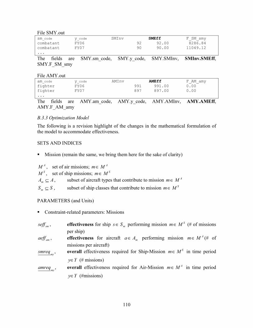
File SMY.out sm_code y_code SMInv SMEff F_SM_smy combatant FY06 92 92.00 8286.84 combatant FY07 90 90.00 11049.12 ...
The fields are SMY.sm_code, SMY.y_code, SMY.SMInv, SMInv.SMEff, SMY.F_SM_smy File AMY.out am_code y_code AMInv AMEff F_AM_amy fighter FY06 991 991.00 0.00 fighter FY07 897 897.00 0.00 ...
The fields are AMY.am_code, AMY.y_code, AMY.AMInv, AMY.AMEff, AMY.F_AM_amy
B.3.3 Optimization Model
The following is a revision highlight of the changes in the mathematical formulation of the model to accommodate effectiveness. SETS AND INDICES Mission (remain the same, we bring them here for the sake of clarity)
AM , set of air missions; AMm ∈SM , set of ship missions; SMm ∈
AAm ⊆ , subset of aircraft types that contribute to mission AMm ∈
SSm ⊆ , subset of ship classes that contribute to mission SMm ∈ PARAMETERS (and Units) Constraint-related parameters: Missions
smseff , effectiveness for ship mSs ∈ performing mission m (# of missions
per ship)
SM∈
amaeff , effectiveness for aircraft mAa ∈ performing mission (# of missions per aircraft)
AMm ∈
,my
smreq overall effectiveness required for Ship-Mission in time period
(# missions)
SMm ∈
Yy∈,
myamreq overall effectiveness required for Air-Mission in time period
(#missions)
AMm ∈
Yy∈
110
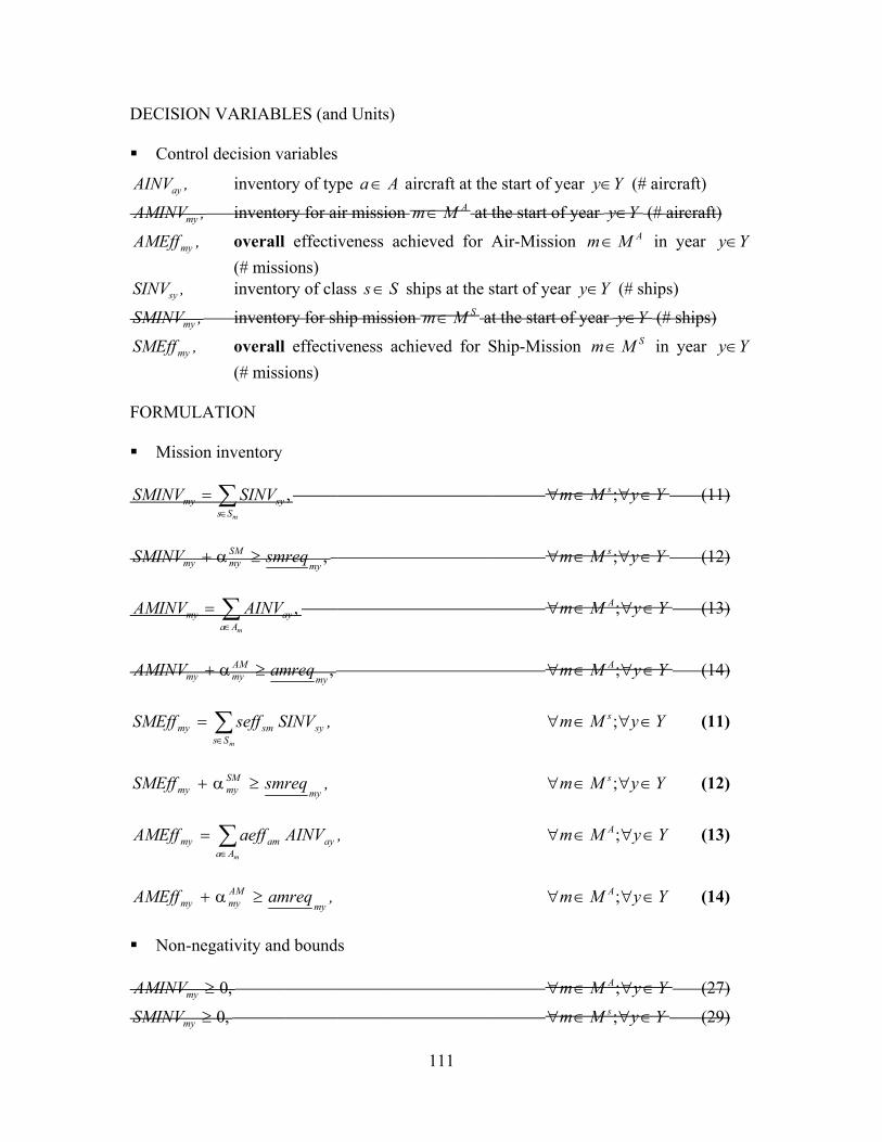
DECISION VARIABLES (and Units) Control decision variables
,AINVay inventory of type Aa ∈ aircraft at the start of year Yy∈ (# aircraft)
,AMINVmy inventory for air mission AM∈m at the start of year Yy∈ (# aircraft)
,AMEffmy overall effectiveness achieved for Air-Mission m in year AM∈ Yy∈ (# missions)
,SINVsy inventory of class Ss ∈ ships at the start of year Yy∈ (# ships)
,SMINVmy inventory for ship mission SMm ∈ at the start of year Yy∈ (# ships)
,SMEffmy overall effectiveness achieved for Ship-Mission in year SMm ∈ Yy∈ (# missions)
FORMULATION Mission inventory
,∑
∈
=mSs
symy SINVSMINV YyMm s ∈∀∈∀ ; (11)
,
mySMmymy smreqSMINV ≥α+ YyMm s ∈∀∈∀ ; (12)
,∑
∈
=mAa
aymy AINVAMINV YyMm A ∈∀∈∀ ; (13)
,
myAMmymy amreqAMINV ≥α+ YyMm A ∈∀∈∀ ; (14)
,SINVseffSMEff
mSssysmmy ∑
∈
= ∀ (11) YyMm s ∈∀∈ ;
,smreqSMEff
mySMmymy ≥α+ ∀ (12) YyMm s ∈∀∈ ;
,AINVaeffAMEff
mAaayammy ∑
∈
= ∀ (13) YyMm A ∈∀∈ ;
,amreqAMEff
myAMmymy ≥α+ ∀ (14) YyMm A ∈∀∈ ;
Non-negativity and bounds
,0≥myAMINV YyMm A ∈∀∈∀ ; (27)
,0≥mySMINV YyMm s ∈∀∈∀ ; (29)
111

,AMEffmy 0≥ ∀ (27) YyMm A ∈∀∈ ;
,SMEffmy 0≥ ∀ (29) YyMm s ∈∀∈ ;
B.3.4 Heuristic Source Files
CIPA_DAT.fi: Define new data: SEff(s,sm), AEff(a,am) CIPA_RES.fi: Define new results: SMff(sm,y), AMEff(am,y) READ_AAM.f: Read AEff(a,am); Check consistency AEff(a,am)≥0;
Assign Aircraft-to-Mission iff AEff(a,am)>0;
GAMS_SSM.f: Add writing a new file, Par_SSM.dat containing AEff(a,am)
B.3.5 GAMS Source Files
Par_SSM.gms (New): GAMS file to read SEff(s,sm)
READ_SSM.f: Read SEff(s,sm); Check consistency SEff(s,sm)≥0; Assign Ship-to-Mission iff SEff(s,sm)>0;
CIPA_ERR.fi: Add data errors to the error list:
Msg(287)=SSM_dat//': It must be SEff >= 0' Msg(327)=AAM_dat//': It must be AEff >= 0'
LB_AM.f: Compute maximum possible Air-Mission effectiveness
Max_AMEff and calculate the Air-Mission lower bound LB_SM.f: Compute maximum possible Ship-Mission effectiveness
Max_SMEff and calculate the Ship-Mission lower bound UP_AMINV.f: Update Air-Mission effectiveness UP_SMINV.f: Update Ship-Mission effectiveness UP_F_AM_amy.f: Update cost of Air-Mission effectiveness instead of inventory UP_F_SM_smy.f: Update cost of Ship-Mission effectiveness instead of inventory GAMS_AAM.f: Add writing a new file, Par_AAM.dat containing AEff(a,am)
Par_AAM.gms (New): GAMS file to read AEff(a,am)
Vars.gms: Positive decision variables AMEff(am,y) and SMEff(sm,y) substitute
AMInv(am,y) and SMInv(sm,y) Eqs.gms: Equations SMiss_1, SMiss_2, AMiss_1, AMiss_2 (eqs. (11) to
(14) of the model, respectively) must be modified according to the new eqs. (11) to (14)
112
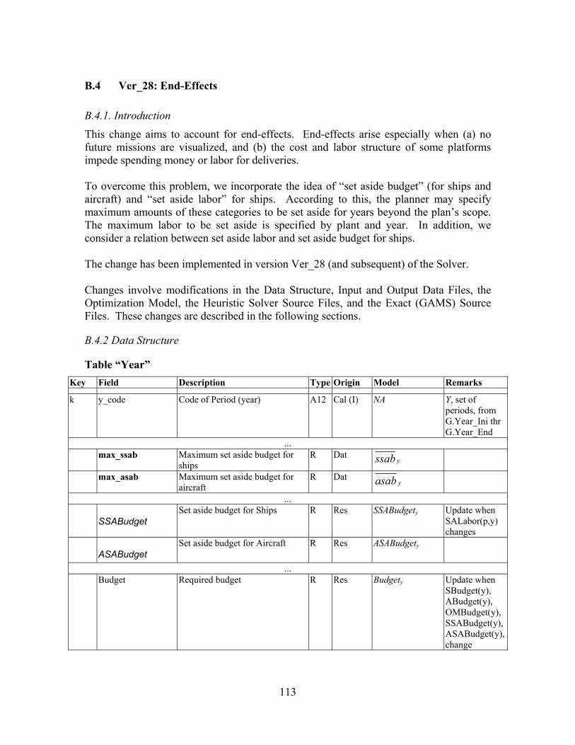
B.4 Ver_28: End-Effects
B.4.1. Introduction
This change aims to account for end-effects. End-effects arise especially when (a) no future missions are visualized, and (b) the cost and labor structure of some platforms impede spending money or labor for deliveries. To overcome this problem, we incorporate the idea of “set aside budget” (for ships and aircraft) and “set aside labor” for ships. According to this, the planner may specify maximum amounts of these categories to be set aside for years beyond the plan’s scope. The maximum labor to be set aside is specified by plant and year. In addition, we consider a relation between set aside labor and set aside budget for ships. The change has been implemented in version Ver_28 (and subsequent) of the Solver. Changes involve modifications in the Data Structure, Input and Output Data Files, the Optimization Model, the Heuristic Solver Source Files, and the Exact (GAMS) Source Files. These changes are described in the following sections.
B.4.2 Data Structure
Table “Year” Key Field Description Type Origin Model Remarks
k y_code Code of Period (year) A12 Cal (I) NA Y, set of periods, from G.Year_Ini thr G.Year_End
... max_ssab Maximum set aside budget for
ships R Dat
yssab
max_asab Maximum set aside budget for aircraft
R Dat yasab
...
SSABudget Set aside budget for Ships R Res SSABudgety Update when
SALabor(p,y) changes
ASABudget
Set aside budget for Aircraft R Res ASABudgety
Budget Required budget R Res Budgety Update when SBudget(y), ABudget(y), OMBudget(y), SSABudget(y),ASABudget(y), change
...
113
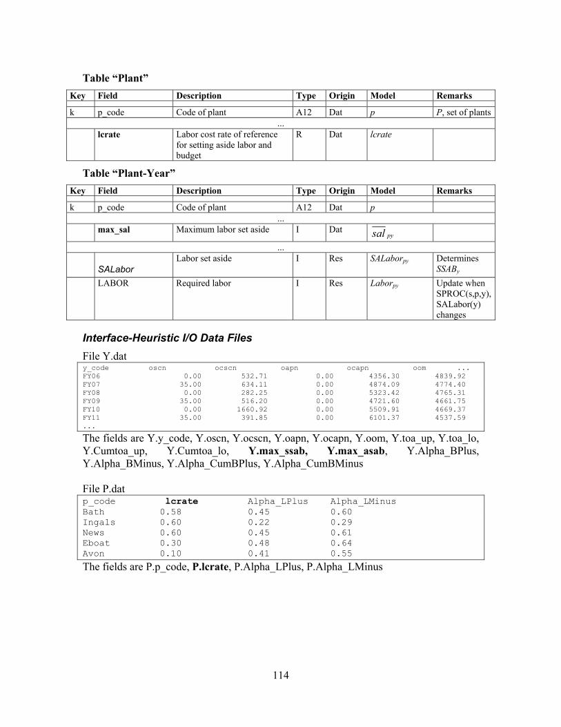
Table “Plant” Key Field Description Type Origin Model Remarks
k p_code Code of plant A12 Dat p P, set of plants...
lcrate Labor cost rate of reference for setting aside labor and budget
R Dat lcrate
Table “Plant-Year” Key Field Description Type Origin Model Remarks
k p_code Code of plant A12 Dat p
max_sal Maximum labor set aside I Dat pysal
...
SALabor Labor set aside I Res SALaborpy Determines
SSABy
LABOR Required labor I Res Laborpy Update when SPROC(s,p,y), SALabor(y) changes
...
Interface-Heuristic I/O Data Files File Y.dat y_code oscn ocscn oapn ocapn oom ... FY06 0.00 532.71 0.00 4356.30 4839.92 FY07 35.00 634.11 0.00 4874.09 4774.40 FY08 0.00 282.25 0.00 5323.42 4765.31 FY09 35.00 516.20 0.00 4721.60 4661.75 FY10 0.00 1660.92 0.00 5509.91 4669.37 FY11 35.00 391.85 0.00 6101.37 4537.59 ...
The fields are Y.y_code, Y.oscn, Y.ocscn, Y.oapn, Y.ocapn, Y.oom, Y.toa_up, Y.toa_lo, Y.Cumtoa_up, Y.Cumtoa_lo, Y.max_ssab, Y.max_asab, Y.Alpha_BPlus, Y.Alpha_BMinus, Y.Alpha_CumBPlus, Y.Alpha_CumBMinus File P.dat p_code lcrate Alpha_LPlus Alpha_LMinus Bath 0.58 0.45 0.60 Ingals 0.60 0.22 0.29 News 0.60 0.45 0.61 Eboat 0.30 0.48 0.64 Avon 0.10 0.41 0.55
The fields are P.p_code, P.lcrate, P.Alpha_LPlus, P.Alpha_LMinus
114
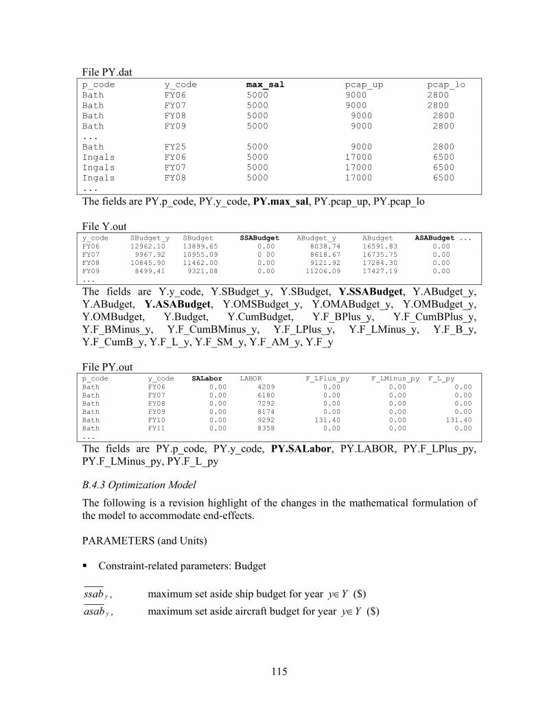
File PY.dat p_code y_code max_sal pcap_up pcap_lo Bath FY06 5000 9000 2800 Bath FY07 5000 9000 2800 Bath FY08 5000 9000 2800 Bath FY09 5000 9000 2800 ... Bath FY25 5000 9000 2800 Ingals FY06 5000 17000 6500 Ingals FY07 5000 17000 6500 Ingals FY08 5000 17000 6500 ...
The fields are PY.p_code, PY.y_code, PY.max_sal, PY.pcap_up, PY.pcap_lo File Y.out y_code SBudget_y SBudget SSABudget ABudget_y ABudget ASABudget ... FY06 12962.10 13899.65 0.00 8038.74 16591.83 0.00 FY07 9967.92 10955.09 0 00 8618.67 16735.75 0.00 FY08 10845.90 11462.00 0.00 9121.92 17284.30 0.00 FY09 8499.41 9321.08 0.00 11206.09 17427.19 0.00 ...
The fields are Y.y_code, Y.SBudget_y, Y.SBudget, Y.SSABudget, Y.ABudget_y, Y.ABudget, Y.ASABudget, Y.OMSBudget_y, Y.OMABudget_y, Y.OMBudget_y, Y.OMBudget, Y.Budget, Y.CumBudget, Y.F_BPlus_y, Y.F_CumBPlus_y, Y.F_BMinus_y, Y.F_CumBMinus_y, Y.F_LPlus_y, Y.F_LMinus_y, Y.F_B_y, Y.F_CumB_y, Y.F_L_y, Y.F_SM_y, Y.F_AM_y, Y.F_y File PY.out p_code y_code SALabor LABOR F_LPlus_py F_LMinus_py F_L_py Bath FY06 0.00 4209 0.00 0.00 0.00 Bath FY07 0.00 6180 0.00 0.00 0.00 Bath FY08 0.00 7292 0.00 0.00 0.00 Bath FY09 0.00 8174 0.00 0.00 0.00 Bath FY10 0.00 9292 131.40 0.00 131.40 Bath FY11 0.00 8358 0.00 0.00 0.00 ...
The fields are PY.p_code, PY.y_code, PY.SALabor, PY.LABOR, PY.F_LPlus_py, PY.F_LMinus_py, PY.F_L_py
B.4.3 Optimization Model
The following is a revision highlight of the changes in the mathematical formulation of the model to accommodate end-effects. PARAMETERS (and Units) Constraint-related parameters: Budget
,ssab y maximum set aside ship budget for year Yy∈ ($) ,asab y maximum set aside aircraft budget for year Yy∈ ($)
115
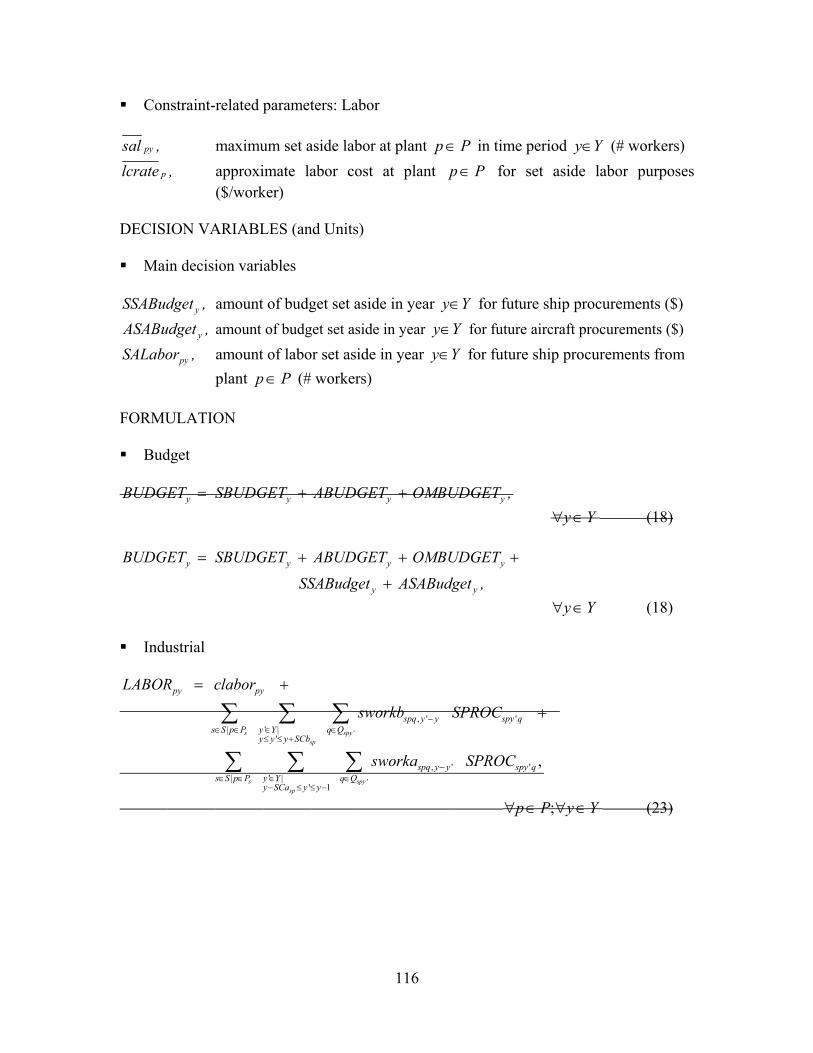
Constraint-related parameters: Labor
,sal py maximum set aside labor at plant Pp ∈ in time period (# workers) Yy∈
, approximate labor cost at plant lcrate p Pp ∈ for set aside labor purposes ($/worker)
DECISION VARIABLES (and Units) Main decision variables
,SSABudget y amount of budget set aside in year Yy∈ for future ship procurements ($) , amount of budget set aside in year ASABudget y Yy∈ for future aircraft procurements ($)
,SALaborpy amount of labor set aside in year Yy∈ for future ship procurements from plant (# workers)
Pp ∈ FORMULATION Budget
,OMBUDGETABUDGETSBUDGETBUDGET yyyy ++= Yy ∈∀ (18)
,ASABudgetSSABudget
OMBUDGETABUDGETSBUDGETBUDGET
yy
yyyy
+
+++=
Yy ∈∀ (18) Industrial
'
, ' '| ' |
'
s spy
sp
py py
spq y y spy qs S p P y Y q Q
y y y SCb
LABOR clabor
sworkb SPROC−∈ ∈ ∈ ∈
≤ ≤ +
= +
+∑ ∑ ∑
'
, ' '| ' |
' 1
,s spy
sp
spq y y spy qs S p P y Y q Q
y SCa y y
sworka SPROC−∈ ∈ ∈ ∈
− ≤ ≤ −
∑ ∑ ∑
YyPp ∈∀∈∀ ; (23)
116
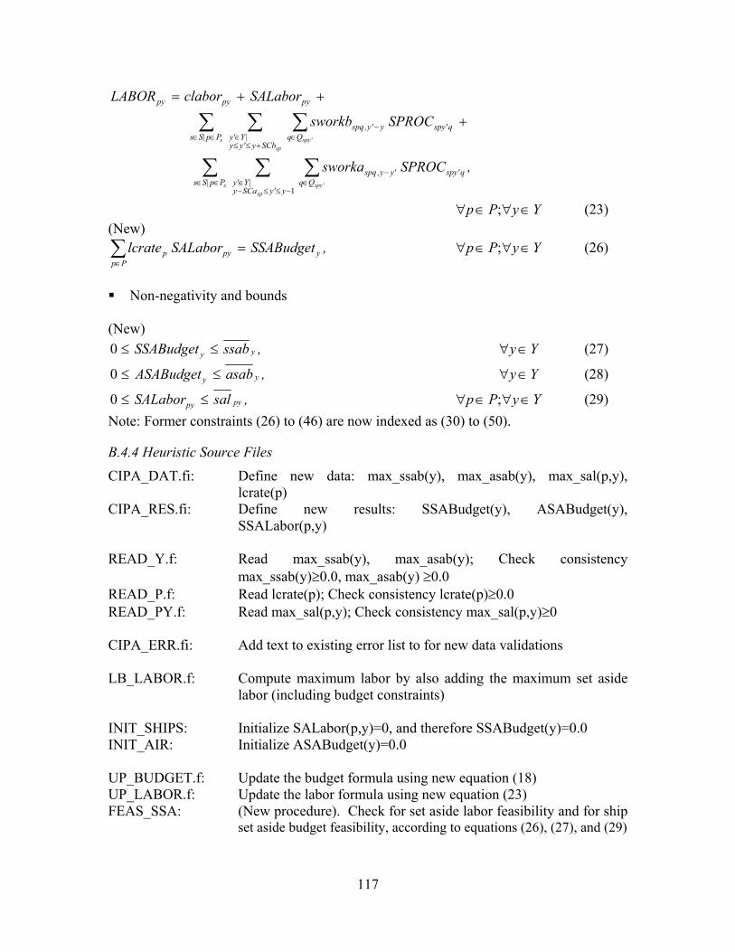
,SPROCsworka
SPROCsworkb
SALaborclaborLABOR
ssp
'spy
ssp
'spy
Pp|Ssy'ySCay
|Y'y Qqq'spy'yy,spq
Pp|SsSCby'yy
|Y'y Qqq'spyy'y,spq
pypypy
∑ ∑ ∑
∑ ∑ ∑
∈∈−≤≤−
∈ ∈−
∈∈+≤≤
∈ ∈− +
++=
1
YyPp ∈∀∈∀ ; (23) (New)
,SSABudgetSALaborlcrate yPp
pyp =∑∈
YyPp ∈∀∈∀ ; (26)
Non-negativity and bounds
(New)
, ssabSSABudget yy ≤≤0 Yy ∈∀ (27)
,asabASABudget yy ≤≤0 Yy ∈∀ (28)
,salSALabor pypy ≤≤0 YyPp ∈∀∈∀ ; (29)
READ_PY.f: Read max_sal(p,y); Check consistency max_sal(p,y)≥0
Note: Former constraints (26) to (46) are now indexed as (30) to (50).
B.4.4 Heuristic Source Files
CIPA_DAT.fi: Define new data: max_ssab(y), max_asab(y), max_sal(p,y), lcrate(p)
CIPA_RES.fi: Define new results: SSABudget(y), ASABudget(y), SSALabor(p,y)
READ_Y.f: Read max_ssab(y), max_asab(y); Check consistency
max_ssab(y)≥0.0, max_asab(y) ≥0.0 READ_P.f: Read lcrate(p); Check consistency lcrate(p)≥0.0
CIPA_ERR.fi: Add text to existing error list to for new data validations LB_LABOR.f: Compute maximum labor by also adding the maximum set aside
labor (including budget constraints) INIT_SHIPS: Initialize SALabor(p,y)=0, and therefore SSABudget(y)=0.0 INIT_AIR: Initialize ASABudget(y)=0.0 UP_BUDGET.f: Update the budget formula using new equation (18) UP_LABOR.f: Update the labor formula using new equation (23) FEAS_SSA: (New procedure). Check for set aside labor feasibility and for ship
set aside budget feasibility, according to equations (26), (27), and (29)
117

FEAS_ASA: (New procedure). Check for aircraft set aside budget feasibility, according to equation (28)
FEAS_ALL: Needs to call on FEAS_SSA and FEAS_ASA (in addition to previous feasibility procedures) in order to validate any given solution
SET_ASIDE.f: To manage the set aside strategies SET_ASIDE_INI: To calculate a reasonable incremental rate to determine new set
aside options SET_ASIDE_SHIP: To analyze a variety of new set aside options for labor and ship
budget SET_ASIDE_AIR: To analyze a variety of new set aside options for aircraft budget OPTIMIZE: To call on the SET_ASIDE procedure (in addition to the others
local search strategies) GAMS_Y.f: Add writing parameters max_ssab(y), max_asab(y) to file
Par_Y.dat used by GAMS GAMS_P.f: Add writing parameter lcrate(p) to file Par_P.dat used by GAMS GAMS_PY.f: Add writing parameter max_sal(p,y) to file Par_PY.dat used by
GAMS READ_GAMS_Y.f: Add reading results SSABudget(y), ASABudget(y) from file
\gams\results\Y.out after GAMS optimization READ_GAMS_PY.f: Add reading results SALabor(p,y), from file \gams\results\PY.out
after GAMS optimization WRITE_G.f: Add printing the timing of the SET_ASIDE procedure to G.out WRITE_Y.f: Add printing the solution SSABudget(y), ASABudget(y) to Y.out WRITE_PY.f: Add printing the solution SSALabor(p,y) to PY.out
Par_P.gms: Read also lcrate(p)
B.4.5 GAMS Source Files
Par_Y.gms: Read also max_ssab(y), max_asab(y)
Par_PY.gms: Read also max_sal(p,y) Vars.gms: Positive decision variables SSABudget(y), ASABudget(y),
SSALabor(p,y) Eqs.gms: Add equation Labor_4 to represent the new constraint (26).
Modify constraints Budget_1 and Labor_1 according to the new equations (18) and (23), respectively.
Bou_vars.gms: Add bounds for new variables, equations (27)-(29) Round_Parameters.gms: Add parameter r_SALabor(p,y) for rounding SALabor(p,y)
variable to an integer value Round_Fix.gms: Round SALabor(p,y) to its integer part and fix it before resolving
118
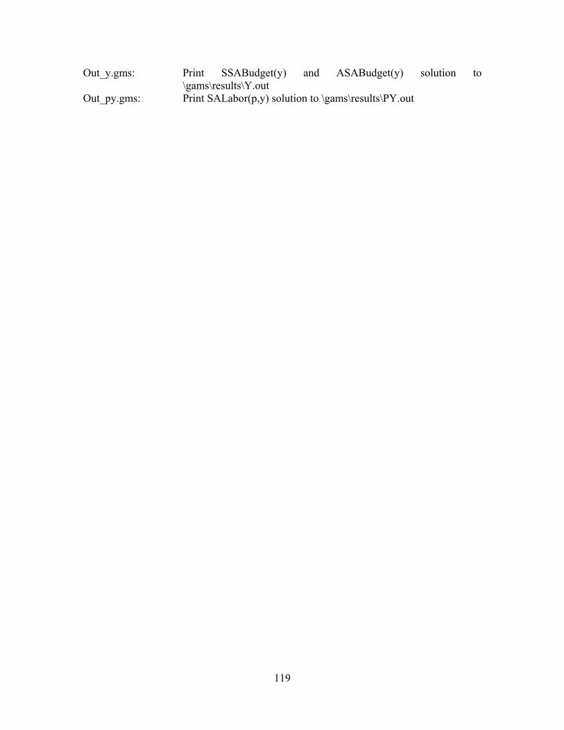
Out_y.gms: Print SSABudget(y) and ASABudget(y) solution to \gams\results\Y.out
Out_py.gms: Print SALabor(p,y) solution to \gams\results\PY.out
119
References Baker, S., [2001], “Unmanned Air Combat Vehicle 2010,” Air Force Materiel Command
News Service, September 24. Baran, N., [2000], “Optimizing Procurement Planning of Navy Ships and Aircraft,” MS
Thesis in Operations Research, Naval Postgraduate School, Monterey, CA, December.
Boeing [2001], An artist’s rendition of the Boeing Unmanned Combat Air Vehicle
(UCAV). [http://www.Boeing.com], accessed August. Brooke, A., Kendrick, D., Meeraus, A., and Raman, R., [1998], “GAMS User’s Guide,”
GAMS Development Corporation, Washington, DC. Capaccio, T., [2001], “Emergency Defense Funds Going To Improve Military
Intelligence,” [http://www.Bloomberg.com], accessed September 27. Chief of Naval Operations, [2000], “Vision..Presence..Power-A Program Guide to the
U.S. Navy, 2000 Edition,” [http://www.chinfo.navy.mil/navpalib/policy/vision/ Vis00/v00-ch2b.html], accessed March 2002.
CIPA: Data Structures [2002], Naval Postgraduate School (development document). CIPA: Quick Tour [2001], Naval Postgraduate School (PowerPoint presentation). CIPA Solver Versions [2002], Naval Postgraduate School (development document). CIPA: User’s Manual [2001], Naval Postgraduate School (in preparation). Digital Visual Fortran [1998], Professional Edition 6.0.0., Digital Equipment
Corporation. Field, R., [1999], “Planning Capital Investment in Navy Forces,” MS Thesis in
Operations Research, Naval Postgraduate School, Monterey, CA, December. GAMS/CPLEX, [2002], [http://www.gams.com/solvers/solvers.htm#CPLEX], accessed
February 7. GAMS/OSL [2002], [http://www.gams.com/solvers/solvers.htm#OSL], accessed
February 7.
Garcia, R. M., [2001], “Optimized Procurement and Retirement Planning of Navy Ships and Aircraft,” MS Thesis in Operations Research, Naval Postgraduate School, Monterey, CA, December.
120
Grossman, E. M., [2001], “Rumsfeld Changes Yardstick For Measuring And Shaping U.S. Forces,” Inside The Pentagon, July 26.
Hagan, K. J., [1978], In Peace and War: Interpretations of American Naval History,
1775-1978, Greenwood Press, Westpoint, Connecticut. ILOG [2002], “ILOG CPLEX,” [http://www.ilog.com/products/cplex/], accessed
February 7. Lockheed Martin, [2001], An artist’s rendition of the Lockheed Martin Joint Strike
Fighter (JSF). Martin, L.W., [1988], “Economics of War,” appears in Encyclopedia Britannica, ed.
Britannica Editors, Encyclopaedia Britannica, Inc. Microsoft Excel [2002], Microsoft Corporation,
[http://www.microsoft.com/office/excel/default.htm], accessed February 7. Navy Public Affairs Library, [1997], “F/A-18 E/F Super Hornet,” The Navy Office of
Information, http://www.chinfo.navy.mil/navpalib/, accessed August 2001. Navy Public Affairs Library, [2000], “At Least Six Sailors Killed in Small Boat Attack
on USS Cole,” The Navy Office of Information, October 1. Pasztor, A., Squeo, A. M., and Rogers, D., [2001], “Boeing Could Be First to Benefit
From Growing Defense Spending,” Wall Street Journal, October 2. OSL [2002], “IBM OSL,” [http://www-4.ibm.com/software/data/bi/osl/], accessed
February 7. Rhem, K., [2001], “Bush: No Distinction Between Attackers and Those Who Harbor
Them,” American Forces Press Service, September 11. Scarborough, R., [2001a], “Bush's 'Strategy First' Vow Scrapped, Review Officials Say,”
Washington Times, July 23. Scarborough, R., [2001b], “Defense Review To Feel Impact Of Terror Attacks,”
Washington Times, September 27. Thomas, C., [2001], “Rumsfeld's New Defense Strategies,” Washington Times, August 1. System Planning and Analysis (SPA), [2000], “SPA Briefing to Naval Center for Cost
Analysis—SPA Extended Planning Annex Model,” briefing presented to Naval Center for Cost Analysis, Washington, DC, March 16.
121
USS CONSTITUTION, [1999], “Old Ironsides History Page,” [http://www.ussconstitution.navy.mil/Shiphistoryx.thm], December.
Valentine, W., [1999], “The IWAR/CPAM Assessment Process,” briefing presented to
the Naval Postgraduate School, Monterey, CA, March 18. Weinberger, S., [2001], “Wolfowitz Promises Paradigm Shift With QDR, But Offers Few
Details,” Aerospace Daily, August 9. Whittle, R., [2001], “Defense Bill May Force V-22 Production Cuts,” Dallas Morning
News, September 8. Windows 2000 [2002], Microsoft Corporation,
[http://www.microsoft.com/windows2000/], accessed February 7.
122
Initial Distribution List
1. Research Office (Code 09).............................................................................................1 Naval Postgraduate School Monterey, CA 93943-5000
2. Dudley Knox Library (Code 013)..................................................................................2 Naval Postgraduate School Monterey, CA 93943-5002
3. Defense Technical Information Center..........................................................................2 8725 John J. Kingman Rd., STE 0944 Ft. Belvoir, VA 22060-6218
4. Richard Mastowski (Editorial Assistant) .......................................................................2 Department of Operations Research Naval Postgraduate School Monterey, CA 93943-5000
5. Research Assistant Professor Javier Salmeron ..............................................................3 Department of Operations Research Naval Postgraduate School Monterey, CA 93943-5000
6. Associate Professor Robert F. Dell................................................................................3 Department of Operations Research Naval Postgraduate School Monterey, CA 93943-5000
7. Distinguished Professor Gerald G. Brown.....................................................................3 Department of Operations Research Naval Postgraduate School Monterey, CA 93943-5000
8. Research Associate Anton Rowe ...................................................................................3 Department of Operations Research Naval Postgraduate School Monterey, CA 93943-5000
9. Chief of Naval Operations (N81)...................................................................................1 ATTN: CDR Steve Richter 2000 Navy Pentagon Washington, DC 20350-2000
123

10. Chief of Naval Operations (N81)...................................................................................1 ATTN: Mr. Mike Albright 2000 Navy Pentagon Washington, DC 20350-2000
11. Chief of Naval Operations (N81)...................................................................................1 ATTN: Mr. Greg Melcher 2000 Navy Pentagon Washington, DC 20350-2000
12. Chief of Naval Operations (N81)...................................................................................1 2000 Navy Pentagon Washington, DC 20350-2000
124