Can Monetary Policy Make Foreign Aid More Effective?

Alessandro Prati, Ratna Sahay, and Thierry Tressel1 International Monetary Fund

This version: February 28, 2005

Abstract This paper develops a two-period model to analyze the welfare effects of monetary policy in a typical aid-receiving country. We consider a small open economy with a closed capital account where the tradable sector raises overall productivity through learning-by-doing (LBD) externalities. Front-loading consumption aid increases current consumption but reduces future productivity as real exchange appreciation shrinks the tradable sector. Front-loading productivity-enhancing aid can offset some of these undesired effects of real appreciation. When donors do not disburse aid optimally over time, monetary policy can improve welfare by targeting an interest rate that makes agents replicate the optimal allocation through a decentralized equilibrium. The welfare-improving monetary policy can be either contractionary or expansionary and trades off the benefits of current consumption against those of future consumption and productivity growth. A closed capital account and LBD externalities explain why monetary policy has permanent effects on real variables. Insufficient international reserves can, however, limit its effectiveness. JEL Classification Numbers: O11, O4, O23, E5, F35. Keywords: Aid Effectiveness, Monetary Policy, Real exchange Rate, Dutch Disease. Author’s e-mail address: aprati@imf.org, rsahay@imf.org, and ttressel@imf.org

1 Research Department, International Monetary Fund, 700 19th street N.W., Washington DC 20431. We thank, without implication, Oya Celasun, Tito Cordella, Poonam Gupta, Peter Heller, Olivier Jeanne, Leslie Lipschitz, Alessandro Rebucci, Marta Ruiz-Arranz, Arvind Subramanian for useful comments. Manzoor Gill and Albana Vokshi provided excellent research assistance. The views are those of the authors and do not necessarily represent those of the IMF or IMF policy.

-2-

I. INTRODUCTION

Can monetary policy make foreign aid more (or less) effective? This question has received only cursory attention in the development literature. There is some evidence that low inflation enhances the impact of aid on growth.2 There is also a well-known, but loosely related, literature showing that inflation has negative effects on growth.3 These contributions focus somewhat narrowly on inflation and are predominantly empirical, leaving substantial scope for this paper’s theoretical analysis of the channels through which monetary policy operates in aid-receiving countries.

Exploring the role of monetary policy in aid-receiving countries remains worthwhile

even in the face of the rapidly growing literature asserting the dominant role of institutions in development. Easterly and Levine (2003) and Rodrik at al. (2004), for example, find that, once economic and political institutions are taken into account, policies have little or no role in explaining long-run growth. From this perspective, paying attention only to monetary policy, as we do in this paper, might appear limited. Nonetheless, given that institutional changes take a long time, policymakers still need to assess the welfare implications of monetary policy for a given set of institutions. Indeed, in contrast to the existing empirical literature for which low inflation epitomizes good monetary policy, we show that, in aid-receiving economies, monetary policy’s role goes beyond controlling nominal variables. This suggests that further work is needed to assess the empirical relevance of monetary policy for development.

In a typical aid-receiving country, monetary policy affects not only the level of prices

but also the allocation of resources between tradable and non-tradable sectors and over time, with potentially important welfare implications. Our contribution is to add a monetary sector to a two-period model with stylized, but realistic, effects of aid on consumption and productivity.4 As in most aid-receiving countries, the capital account is closed and government bonds―whose supply the central bank can regulate―are the only interest-bearing financial instruments in the economy.5 This allows monetary policy to affect real 2 Burnside and Dollar (2000, 2004a, 2004b) include inflation―together with fiscal and trade policies―in an index of “good” policies and institutions on which aid effectiveness depends. Easterly, Levine, and Roodman (2004), among others, have raised doubts on the robustness of Burside and Dollar’s evidence.

3 See, for example, Easterly and Fischer (2001).

4 Buffie et al. (2004) also study the interaction between monetary policy and aid inflows. They focus, however, on a permanent increase in aid and do not analyze the supply-side response to it. Moreover, they need to calibrate their model to conduct welfare analysis.

-3-

variables through sales or purchases of government bonds.6 Moreover, we show that in the presence of externalities, monetary policy has permanent effects.

Specifically, we show that the central bank can respond to foreign aid inflows by

undoing some of the associated money supply expansion, thereby preventing real appreciation, preserving the competitiveness of the tradable sector, and raising international reserves and national savings. We find that this policy amounts to postponing consumption aid and that it is welfare-improving only if the economy is better off saving part of the aid for later use.7 Monetary policy can also help if the desired allocation requires bringing aid forward as it happens when immediate consumption benefits of aid are large but disbursements are backloaded. In this case, monetary policy needs to be expansionary and, if the stock of international reserves is large enough, can realize the same resource allocation achievable by frontloading aid.

Krugman (1987) also argued that, in the presence of learning-by-doing externalities,

temporary monetary policies can have permanent effects on competitiveness. However, in his paper, the effect of monetary policy is the exact opposite of what our paper predicts. In Krugman’s model of trade with two economies, sticky prices, and balanced trade, tight money leads to real appreciation. In our model tight money instead leads to real depreciation. Section II.C explains why our results differ. Prati et al. (2003) present some preliminary empirical evidence confirming that, in aid-receiving countries, tighter monetary policy is associated with real depreciation.

We consider three reasons why redistributing the impact of aid over time may improve welfare. First, given aid volatility, postponing or advancing aid disbursements may help smooth consumption. Figure 1 shows that, in several countries, the average annual ratio of net official development assistance (ODA) to GDP is in the 10 to 30 percent range with some massive differences between minimum and maximum annual inflows.8 Average annual

5 Allowing for bank lending to the private sector would not modify our main conclusions, as long as the capital account remains closed.

6 In practice, when there is no domestic bond market, alternative policy measures have been used with equivalent effects on money supply and resource allocation. We discuss these alternatives in Section II.

7 Matsen and Torvik (2004) analyze the optimal spending path of natural resource wealth but do not analyze monetary policy. Moreover, in their paper, individuals’ consumption decisions are constrained by the exogenously set current account, while we endogenize the current account balance under the intertemporal foreign exchange constraint.

8 Bulir and Hamann (2002) discuss the fiscal implications of the volatility and (un)predictability of foreign aid.

-4-

absolute changes can easily exceed 10 percent of GDP and, in some instances, they have plummeted by as much as 30-40 percent of GDP in a single year. These sudden reversals surpass those of net capital inflows in emerging markets, which reached, for example, 13 percent of GDP in Mexico (1993-95) and 24 percent of GDP in Thailand (1996-98).

Second, if aid not only boosts consumption but enhances the productive capacity of

the recipient country, there is an additional benefit from spending it immediately or moving it forward. In our model, we allow for part of aid disbursements to augment directly medium-term productivity, albeit with diminishing marginal returns to reflect absorptive capacity constraints. This is an all-encompassing effect associated to aid-financed public investment. Its real size may vary across time and countries depending on a variety of factors including the quality of economic and political institutions.

Figure 1: ODA flows in percent of GDP during the 1990s (average, minimum, maximum)

-10.0%

0.0%

10.0%

20.0%

30.0%

40.0%

50.0%

60.0%

70.0%

80.0%

90.0%

Algeria

Aruba

Belize

Bolivia

Burund

i

Cape V

erde

Djibou

ti

El Salv

ador

Gabon

Grenad

a

Guinea

-Biss

au

Hondu

ras

Jamaic

a

Kiriba

ti

Mad

agasc

arM

ali

Mau

ritius

Moro

cco Nepal

Nigeria

Parag

uay

Rwanda

Seyc

helle

s

Sri L

anka

Surin

ame

Togo

Ugand

aYem

en

Third, indirect negative effects of aid on productivity may justify deferring the use of

part of it. Among the many reasons put forward in the literature for these negative effects, we consider the so-called Dutch disease. When part of foreign aid is spent on domestic non-tradable goods, the price of non-tradable goods rises relative to tradable goods. This real appreciation draws resources out of the tradable-goods sector into the non-tradable goods sector. While this reallocation is not inefficient per se, the shrinking of the tradable-goods sector will reduce growth if the source of productivity expansion―e.g., learning-by-doing (LBD) externalities―is in the tradable-goods sector. Other negative effects of aid on productivity due, for example, to the corrupting effects of large amounts of aid on the recipient country’s institutions could be easily captured in our stylized model by allowing

-5-

marginal returs of aid not only to diminish but to become negative beyond a certain threshold. Such extension would, of course, tend to increase the benefits from saving aid.

By trading off the consumption and productivity benefits of aid against the costs of

Dutch disease we characterize the optimal distribution of a given net present value of aid over time and the associated optimal time paths of the real exchange rate and the current account. We then show that, provided the initial stock of international reserves is large enough, monetary policy can implement an equivalent resource allocation.

The paper is organized as follows. Section II explains why monetary policy affects

real variables in aid-receiving countries and is more suitable than fiscal policy to respond to volatile aid inflows. Section III presents the structure of the model, discussing key assumptions and related literature. Section IV illustrates partial equilibrium results. Section V analyzes the general equilibrium effects of aid flows and of monetary policy. Section VI determines the optimal timing of foreign aid flows. Section VII concludes. Appendix I outlines the solution strategy of the model and collects all the proofs, including that of existence and unicity of a general equilibrium. Appendix II shows that the results extend to the cases of managed float and flexible exchange rates.

II. MONETARY POLICY IN AID-RECEIVING COUNTRIES

In this section, we justify our assumptions on foreign aid disbursements, capital mobility, and the exchange rate regime. In addition, we describe the conduct of monetary policy in aid-receiving countries and outline the monetary impact of aid inflows. We also explain why, in these countries, monetary policy has effects on real variables and how the results of this paper relate to the literature on aid effectiveness. Finally, we discuss why monetary policy is more suitable than fiscal policy to undo the undesirable effects of a given distribution of aid over time.

A. Foreign aid and capital mobility

We assume that recipient governments cannot save aid directly nor can they borrow against future expected aid disbursements. These assumptions are realistic. Donors usually require recipients to spend development assistance when it is disbursed and aid flows are too uncertain to be pledged as collateral. The extreme volatility of aid inflows suggests that―barring those cases where the surge in aid has the humanitarian purpose of supporting consumption after famine or war―raising national savings when aid spikes and reducing them when aid subsides could smooth consumption and improve welfare. In this paper, we show that, with a closed capital account, monetary policy can replicate the effects of saving aid, or bringing it forward as long as the stock of international reserves is large enough.

-6-

Private sector agents can save part of the rise in income associated with aid inflows as domestic currency cash balances9 or government bonds. In aggregate, however, the private sector can save only by buying interest-bearing government bonds because all seignorage is transferred back to the private sector. A closed capital account prevents agents from buying international bonds. This assumption is critical for the effectiveness of monetary policy because it disconnects domestic from foreign interest rates, deprives the private sector of a saving instrument whose supply would be perfectly elastic, and allows the central bank to affect aggregate demand and national savings by selling or buying government bonds.

How plausible is the assumption of closed capital account? Countries receiving large aid inflows have de facto no access to international capital markets because most of them have high levels of official indebtedness. Moreover, only a handful of aid-receiving countries has no capital account restrictions.10 As a consequence, in the 1990s, the total of inward and outward private portfolio investments of aid-receiving countries was small both in percent of GDP and in relation to exports and imports (Table 1).

Table 1: Private Portfolio Investments in Aid Receiving Countries

median

mininum

maximum

Average 1990s

0.7

0.0

10.3

53.2

18.3

199.5

portfolio investment assets + liabilities

% GDPexports + imports

% GDP

B. Foreign aid and money supply

In most aid-receiving countries, foreign aid inflows do not only affect consumption and productivity but also cause an initial expansion of money supply, which the monetary authorities often try to offset.

9 If we allowed for real money balances in foreign currencies to capture the dollarization of many aid-receiving economies, all results would go through. Details are available from the authors upon request.

10 IMF (2002), “Annual Report on Exchange Arrangements and Exchange Restrictions.”

-7-

Foreign aid, exchange rate regime, and money supply

Aid inflows tend to be associated with money supply expansions. Spending foreign aid requires exchanging foreign-currency-denominated aid into the recipient country’s currency. In fixed exchange rate regimes, international reserves and base money would then increase at impact. This is our benchmark case as the large majority of aid-receiving countries has adopted either a fixed exchange rate regime or a managed float. According to the classification of exchange rate regimes in Reinhart and Rogoff (2004), during all instances of aid inflows greater than 2 percent of GDP in the 1990s, the median exchange rate regime was a de facto crawling peg with freely floating regimes accounting for less than 1 percent of the observations.

Foreign aid is often associated with an increase in base money also in floating

exchange rate regimes. When aid is aimed at budgetary support, the government usually deposits foreign aid at the central bank. Initially, this operation increases both international reserves and government deposits, leaving total base money unchanged. But, as soon as the government draws down the balance on its deposit account at the central bank, net domestic assets and base money increase. Appendix III extends the results of our model to the case of managed float or floating exchange rates.

Monetary policy

The key question addressed in this paper is whether monetary policy should reduce the central bank’s bond holdings (“net domestic assets”) to offset the initial increase in money supply due to aid inflows or, on the contrary, be expansionary. The policy of reducing net domestic assets in response to large foreign aid inflows is dubbed “sterilization” and is a widespread practice among aid-receiving countries. Over the period 1960-1998, we found 704 episodes―out of 1935 episodes of foreign aid inflows greater than 2 percent of GDP―during which net domestic assets fell. More recently, several African countries (Uganda, Tanzania, Mozambique, Ghana, and Ethiopia) have reduced net domestic assets in response to surges in foreign aid. Sterilization policy can take various forms: (i) central bank’s bond sales; (ii) fiscal surpluses or a shift of government deposits from the banking sector to the central bank; (iii) central bank’s issuance of its own debt certificates; (iv) central bank’s direct sale of foreign exchange; or (v) higher reserve requirements, which, for a given level of base money, reduce the money multiplier and overall money supply.

The stylized model of this paper assumes that sterilization is implemented through a

reduction in the central bank’s bond holdings. Open market bond sales are, indeed, becoming common in several low-income countries on the heels of a rapid development of domestic debt markets (Christensen, 2004). In our model, other sterilization methods would have qualitatively similar effects and all results of the paper would carry through.

In our model, sterilization is costless as interest payments are financed through lump-

sum taxes. In practice, there might be sterilization costs associated with distortionary taxes needed to finance interest payments or fiscal surpluses. The banking system may also loose

-8-

competitiveness as reserve requirements rise. In Section III.C, we discuss the implications of allowing for sterilization costs in our model.

C. How does monetary policy affect real variables?

In a fixed exchange rate regime, sterilization operates in the following way. The central bank reduces its net domestic assets, and thus overall money supply, by selling government bonds. As a result, interest rates increase, agents reduce consumption, the current account improves, and there is accumulation of international reserves. Moreover, the price of non-tradable goods falls to maintain the equilibrium on the non-tradable goods market, so that the real exchange rate depreciates relative to the case with no sterilization.

The creation of base money through the improved current account and accumulation

of foreign exchange reserves feeds back into the money supply and partially offsets the impact of the initial sale of government bonds. This offset is only partial because the demand for nontradables also falls and the improvement in the current account is smaller than the reduction in aggregate demand. Moreover, the closed capital account prevents capital inflows from fully offsetting the initial reduction in money supply.

Monetary policy is non-neutral in the short-run even though prices of nontradable

goods are fully flexible, as in Edwards (1988) and Calvo et al. (1995).11 In a way, this effectiveness reflects the stickiness of tradable goods prices, which remain unchanged in the international markets as monetary policy varies because the supply of tradable goods is perfectly elastic. In addition, in our model, temporary real effects of monetary policy become permanent thanks to the presence of LBD externalities in the tradable sector. The LBD externality depends on the size of the tradable goods sector which, in turn, is a function of the real exchange rate. Temporary effects of sterilization on the real exchange rate translate then into permanent effects on growth through changes in the size of the tradable goods sector.

Krugman (1987) presents a model with two large countries in which learning-by-

doing externalities allow monetary policy to have permanent real effects when wages are sticky and the current account is balanced. In his model, however, monetary tightening causes real appreciation and, therefore, tends to exacerbate Dutch disease problems. This happens because monetary tightening changes relative prices of non-tradable and tradable goods only through changes in the nominal exchange rate, which has to appreciate to rebalance the current account (exports must become less competitive and fall to offset the reduction in imports). If this effect is large enough, the loss of export competitiveness may become permanent as some industries move from the home to the foreign country. By contrast, in our model, monetary tightening puts downward pressure on nontradable prices 11 We assume flexible prices of non-tradable goods in view of the evidence—presented in Reinhart and Rogoff (2004)—that several aid-receiving African countries have experienced long and repeated periods of deflation.

-9-

and the real exchange rate as the effect of the lower demand for non-tradable goods dominates the feedback effect of lower imports on the money supply. As a result, the real exchange rate remains more depreciated and the current account improves.

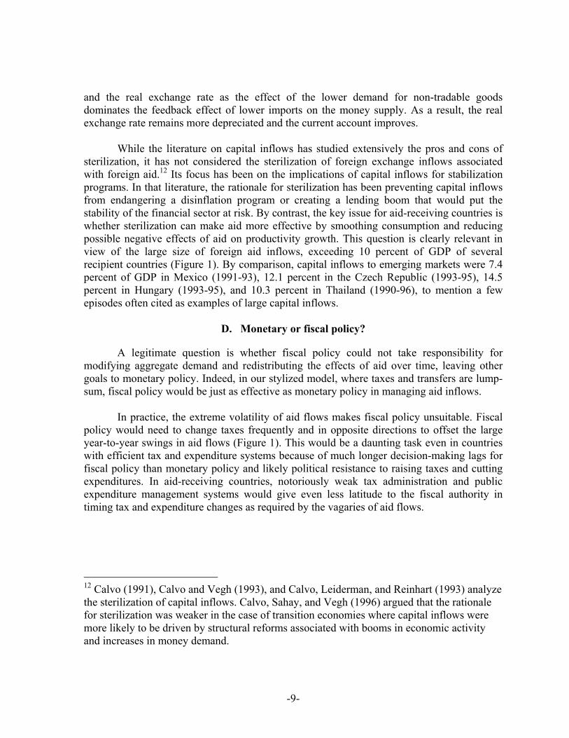
While the literature on capital inflows has studied extensively the pros and cons of

sterilization, it has not considered the sterilization of foreign exchange inflows associated with foreign aid.12 Its focus has been on the implications of capital inflows for stabilization programs. In that literature, the rationale for sterilization has been preventing capital inflows from endangering a disinflation program or creating a lending boom that would put the stability of the financial sector at risk. By contrast, the key issue for aid-receiving countries is whether sterilization can make aid more effective by smoothing consumption and reducing possible negative effects of aid on productivity growth. This question is clearly relevant in view of the large size of foreign aid inflows, exceeding 10 percent of GDP of several recipient countries (Figure 1). By comparison, capital inflows to emerging markets were 7.4 percent of GDP in Mexico (1991-93), 12.1 percent in the Czech Republic (1993-95), 14.5 percent in Hungary (1993-95), and 10.3 percent in Thailand (1990-96), to mention a few episodes often cited as examples of large capital inflows.

D. Monetary or fiscal policy?

A legitimate question is whether fiscal policy could not take responsibility for modifying aggregate demand and redistributing the effects of aid over time, leaving other goals to monetary policy. Indeed, in our stylized model, where taxes and transfers are lump-sum, fiscal policy would be just as effective as monetary policy in managing aid inflows.

In practice, the extreme volatility of aid flows makes fiscal policy unsuitable. Fiscal

policy would need to change taxes frequently and in opposite directions to offset the large year-to-year swings in aid flows (Figure 1). This would be a daunting task even in countries with efficient tax and expenditure systems because of much longer decision-making lags for fiscal policy than monetary policy and likely political resistance to raising taxes and cutting expenditures. In aid-receiving countries, notoriously weak tax administration and public expenditure management systems would give even less latitude to the fiscal authority in timing tax and expenditure changes as required by the vagaries of aid flows.

12 Calvo (1991), Calvo and Vegh (1993), and Calvo, Leiderman, and Reinhart (1993) analyze the sterilization of capital inflows. Calvo, Sahay, and Vegh (1996) argued that the rationale for sterilization was weaker in the case of transition economies where capital inflows were more likely to be driven by structural reforms associated with booms in economic activity and increases in money demand.

-10-

III. THE MODEL

A. Consumers and Prices

We consider a three-goods (exportable, importable, and non-tradable) small open economy lasting two periods13. A continuum of identical individuals consume the importable good ( cT ) and the non-tradable good ( cN ). They also value real money balances of domestic currencies as in the standard money-in-the-utility-function model. For simplicity, we set the subjective discount rate to 1.

The representative agent i maximizes:

ii

iiii CP

MCUUV 2

1

1121 logloglog +⎟

⎟⎠

⎞⎜⎜⎝

⎛+=+= χ

where iM1 denotes nominal money balances held between period 1 and period 2 in domestic currencies, and χ is small. Agents do not value money holdings at the end of period 2. An important assumption is that agents have perfect foresight and know the structure of the economy.

The assumption of Cobb-Douglas preferences with respect to tradable and non-tradable goods implies the following consumption index i

tC :

( ) ( ) 1,2 t 1

,, =⋅=−γγ i

tNi

tTi

t ccC

The consumer price index tP is defined as the minimum cost of one unit of the consumption index i

tC :

1,2 t 1,, =⋅= −γγtNtTt ppP

where pT is the price in local currency of one unit of the tradable good and pN is the price of one unit of the non-tradable good. We assume the law of one price to hold for the imported and the exported good:

1,2t *,, =⋅= tTttT pEp and 1,2 t *

,, =⋅= tXttX pEp where pT

* and px* are respectively the price of the imported good and the price of the

exported good in dollars and tE is the nominal exchange rate in period t (domestic currency per dollar). 13 See De Gregorio and Wolf (1994) and Obstfeld and Rogoff (1999), among others, for similar models.

-11-

The real exchange rate te is:

tT

tNt p

pe

,

,=

Hence, the consumer price index tP (t=1,2) is a function of the nominal exchange

rate, the real exchange rate, and the international price of imports:

*,

1tTttt peEP ⋅⋅= −γ (1-1) and (1-2)

The terms of trade tq are defined as:

tT

tXt p

pq

,

,=

Individual i’s budget constraints for periods one and two in domestic currency are:

( ) iiiiii

iiiiii

MTRBrAEICP

TRAEIBMCP

1222222

1111111

1 ++++⋅+=

+⋅+=++ (2-1) and (2-2)

where iB are the domestic bond holdings between period one and two, r is the nominal interest rate on domestic bonds, iI1 and iI 2 are respectively nominal income in period one and two, iTR1 and iTR2 are lump-sum positive or negative net government transfers, and iA1 and iA2 are positive transfers from abroad (foreign aid) expressed in dollars. The nominal exchange rates 1E and 2E are predetermined in a fixed exchange rate regime. Without loss of generality, we will normalize EEE == 21 .

B. Production

The exportable ( yX ) and the non-tradable goods ( yN ) are produced according to production functions with decreasing returns to scale ( 10 << α ):

αtXtXtX Lay ,,, ⋅= (3-1) and (3-2) α

tNtNtN Lay ,,, ⋅= (4-1) and (4-2) where tiL , (i=X,N) are labor inputs in the exportable and non-tradable sectors.

tNtXt LLL ,, += is the aggregate supply of labor, which is assumed fixed without loss of generality. The productivity parameters are tXa , and tNa , respectively in the exportable and non-tradable sectors. In the following, we will assume that 11,1, aaa XN == .

-12-

We augment this standard specific-factors model―where labor is the only mobile

factor across sectors and there are diminishing returns to labor in each sector―by allowing foreign aid to affect productivity growth. We consider reasons that can make this effect either positive or negative.

Productivity-enhancing aid

Our model allows for a positive effect of aid on productivity associated to aid-financed public spending on, for example, infrastructure, sanitation, education, and health. The vast literature on aid effectiveness has investigated whether this kind of spending has raised recipient countries’ medium-term productivity. The evidence is uneven. Easterly (2001) argues that aid has had little positive effect on growth. By contrast, Clemens et al. (2004) show that certain categories of foreign aid accounting for about 45 percent of aid flows―budget and balance of payments support, investments in infrastructure, and aid for sectors such as agriculture and industry―have large effects on short-run growth. Arellano et al. (2002) also present evidence that foreign aid affects investment.

We assume that foreign aid’s productivity-enhancing effect has positive but

decreasing marginal returns to capture possible absorptive capacity problems. These are related to aid volatility and capacity constraints. Consider the case of projects requiring repeated inputs over the years with donors disbursing aid in a single installment or irregularly. For example, donors would disburse aid to build a school or an hospital but leave recipient countries without a regular source of funds to keep the buildings in good conditions or pay teachers and doctors in the following years. In this case, saving aid to be later spent on maintenance and salaries would ultimately enhance the productivity of the initial investment.

Some empirical studies have found that the marginal returns of foreign aid do not only diminish with size but turn negative beyond a certain threshold (Hansen and Tarp, 2000). This negative impact could be related to the corrupting effects of large amounts of aid on institutions. Tornell and Lane (1998, 1999) stress that powerful groups tend to appropriate windfall earnings, leading to a ‘voracity’ effect. Similarly, Svensson (2000) and Torvik (2002) emphasize how aid may increase rent-seeking. Alesina and Weder (2002) show that, despite these widespread negative effects, donors give aid to honest and corrupt governments alike. We could easily modify the production function of our model to reflect negative marginal productivity benefits of aid; this change would provide an additional rationale for smoothing the effects of aid inflows over time by saving part of them.

We conclude that the actual size and sign of this all-encompassing productivity effect

of aid are likely to vary across time and countries depending on factors such as corruption, institutions, and the internal political process of the recipient country. In our stylized model, a single parameter captures this effect and we can assess the implications of its different values for monetary policy.

-13-

Aid and Dutch disease

Dutch disease usually refers to the adverse effects on the (manufacturing) traded sector of natural resource discoveries, or of foreign aid. Its origin is the overvaluation of the Dutch real exchange rate that followed the discovery of natural gas deposits in the North Sea, within the borders of the Netherlands, in the 1950s and 1960s. Van Wijnbergen (1984), Krugman (1987), Sachs and Warner (1995), and Gylfason et al. (1997) develop, among others, Dutch disease models. These are, usually, real sector models that do not permit an assessment of the role of monetary policy, with the exception of Krugman (1987).

Our model allows for LBD externalities in the traded-goods sector with a perfect

spillover to the rest of the economy. As aid inflows lead to real appreciation and a reallocation of resources from the tradable to the nontradable sector, indirect negative productivity effects can counterbalance the productivity-enhancing impact of aid. In practice, assessing the relevance of each of the two productivity effects requires taking the other into consideration. Education expenditure could, for example, boost the supply of skilled labor, thereby easing wage pressures and potentially lessening Dutch disease concerns.

From the perspective of this paper, an important question is whether the effects of

Dutch disease on productivity growth are really so large that central banks should take them into account in formulating monetary policy. This question needs to be addressed on empirical grounds and answering it fully is beyond the scope of this paper. Almost all studies of aid and Dutch disease are theoretical with only some country-specific and indirect measures of the actual size of a possible negative productivity effect of aid. Adam and Bevan (2003), for example, calibrate a model on Uganda data to show that the impact of aid on the real exchange rate can be complex and may not be large. By contrast, Rajan and Subramanian (2005), however, have recently found that aid has a negative output effect especially in more labor-intensive industries, which is consistent with strong Dutch disease effects.

Dutch disease concerns cannot be easily dismissed by observing that small

manufacturing sectors and commodity-dominated export sectors limit the scope for productivity gains in aid-receiving countries. Manufacturing sectors actually account for non-negligible shares of exports, making up, for example, 15 percent of exports in Tanzania and Kenya, 25 percent in Ghana, and 90 percent in Bangladesh.14 Moreover, manufacturing export shares in several countries that successfully developed over the past 40 years were initially small and comparable to those of today’s aid-receiving countries. In the early sixties, manufacturing exports represented respectively 2, 5, and 20 percent of total exports in Thailand, Malaysia, and Korea. At the end of the nineties, the same shares were 75 percent in Thailand and 90 percent in Malaysia, and Korea. Finally, productivity gains (and/or quality improvements) could take place also in the commodity-exporting sectors because 14 World Bank Development Indicators 2002.

-14-

commodities are often processed domestically to meet international standards, creating some scope for positive LBD spillovers.

There is also no evidence of LBD spillovers in the non-tradable sector of aid-receiving countries that might reduce Dutch disease concerns. Torvik (2001) shows that, if the non-tradable sector is also a source of LBD spillovers, real appreciation has ambiguous implications for growth. This phenomenon is likely to be limited to relatively developed economies where innovation takes place in research centers that can be located either in the tradable or the non-tradable sector. In developing countries, instead, productivity grows mainly through adoption of existing technologies imported from developed economies. Van Biesebroeck (2003) shows that productivity of manufacturing plants in African countries increases after entering export markets. Moreover, in almost all successful export-driven development episodes of the past 40 years, local export industries have increased their productivity by adopting technologies and, occasionally, standards, marketing, and management techniques of developed countries’ industries.

We conclude that, while the empirical relevance of Dutch disease effects associated

to aid inflows may need to be further investigated, we cannot rule it out a priori. Accordingly, we allow for LBD spillovers and discuss how policy prescriptions would change if they were small or absent.

Foreign aid and productivity growth

To capture the productivity-enhancing effects of aid, we introduce an aid-financed public good Px produced in period one that raises period-two productivity in both sectors. To capture the negative productivity effects of Dutch disease, we allow for LBD in the export sector. This is an externality because each firm is too small to take its contribution to LBD into account. We follow Sachs and Warner (1995) by assuming that LBD is generated only in the traded sector and there is a perfect learning spillover to the non-traded sector. The size of the export sector in period one, 1,XL , raises period-two productivity in both sectors:

( ) ( )( ) ( )⎩

⎨⎧

⋅+⋅⋅=

⋅+⋅⋅=

1,1,2,

1,1,2,

11

XNPNN

XXPXX

LzaxhaLzaxha

(5) and (6)

where z is a parameter and h is a function that embodies the decreasing marginal productivity returns of the aid-financed public good, Px :

0>′Xh , 0<′′Xh and 0>′Nh , 0<′′Nh .

Note that, in this stylized version of the model, the lagged effect of Px on productivity prevents any associated positive supply effect from offsetting the real appreciation caused by aid inflows in period one. Moreover, in general, NX hh ≠ : the impact

-15-

of health, education and other productivity improving public expenditures can be sector specific. For simplicity, we focus on the case hhh NX == , and, in view of our assumption

11,1, aaa XN == , this implies that 22,2, aaa XN == .

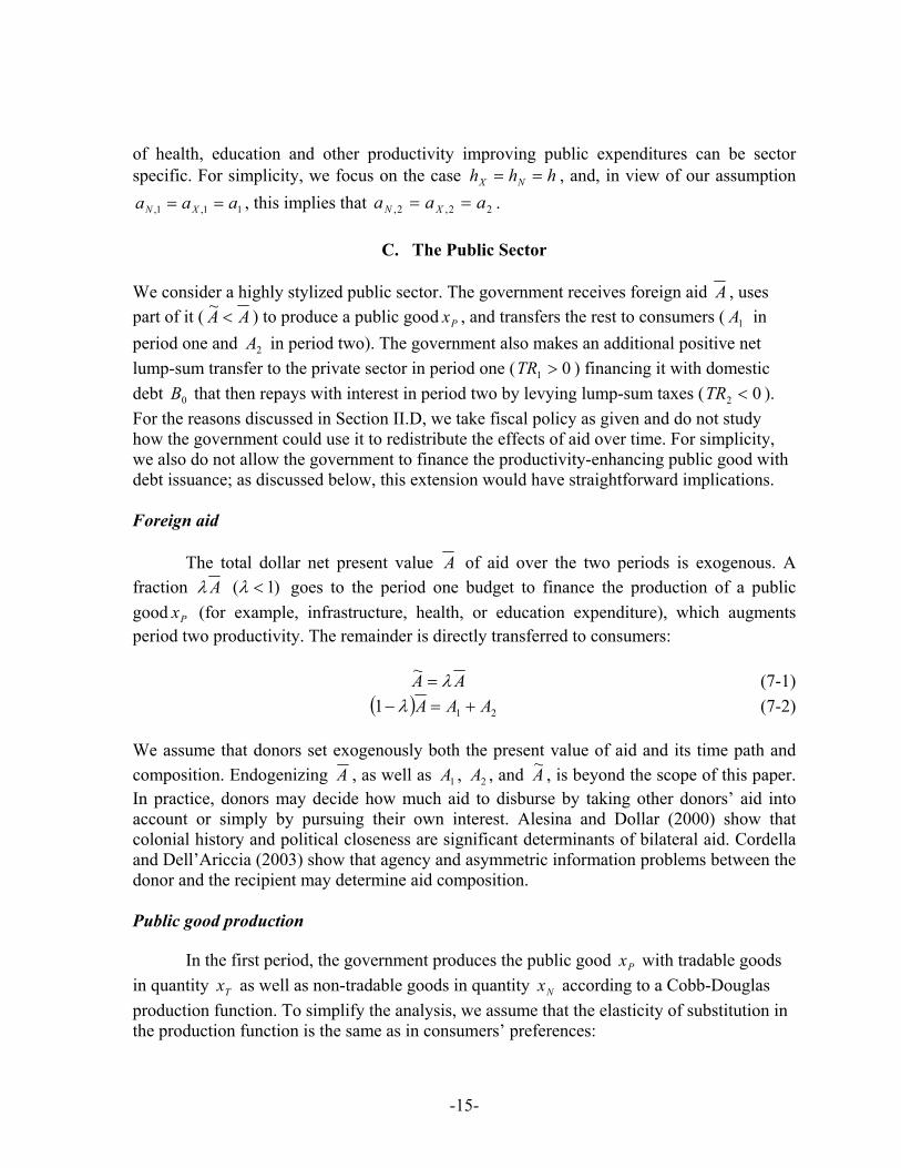
C. The Public Sector

We consider a highly stylized public sector. The government receives foreign aid A , uses part of it ( AA <

~ ) to produce a public good Px , and transfers the rest to consumers ( 1A in period one and 2A in period two). The government also makes an additional positive net lump-sum transfer to the private sector in period one ( 01 >TR ) financing it with domestic debt 0B that then repays with interest in period two by levying lump-sum taxes ( 02 <TR ). For the reasons discussed in Section II.D, we take fiscal policy as given and do not study how the government could use it to redistribute the effects of aid over time. For simplicity, we also do not allow the government to finance the productivity-enhancing public good with debt issuance; as discussed below, this extension would have straightforward implications. Foreign aid

The total dollar net present value A of aid over the two periods is exogenous. A fraction Aλ )1( <λ goes to the period one budget to finance the production of a public good Px (for example, infrastructure, health, or education expenditure), which augments period two productivity. The remainder is directly transferred to consumers:

AA λ=~ (7-1) ( ) 211 AAA +=− λ (7-2)

We assume that donors set exogenously both the present value of aid and its time path and composition. Endogenizing A , as well as 1A , 2A , and A~ , is beyond the scope of this paper. In practice, donors may decide how much aid to disburse by taking other donors’ aid into account or simply by pursuing their own interest. Alesina and Dollar (2000) show that colonial history and political closeness are significant determinants of bilateral aid. Cordella and Dell’Ariccia (2003) show that agency and asymmetric information problems between the donor and the recipient may determine aid composition. Public good production

In the first period, the government produces the public good Px with tradable goods in quantity Tx as well as non-tradable goods in quantity Nx according to a Cobb-Douglas production function. To simplify the analysis, we assume that the elasticity of substitution in the production function is the same as in consumers’ preferences:

-16-

γγTNP xxx ⋅= −1 (8)

This implies that non-tradable and tradable goods are used as inputs in the proportion implied

by consumers’ preferences,γγ

TTNN xpxp=

−1, so that the share of public consumption in total

consumption does not affect the relative demand for tradable and non-tradable goods.

For simplicity, we also assume that the public good is financed only with foreign aid:

Axpxp TTNN~

1,1, =+ (9)

This assumption implies that the government does not use any of the proceeds of domestic debt issuance 0B to finance the production of the public good Px . If we allowed the government to use part of 0B to finance the production of the public good, our conclusions on the role of monetary policy in aid-receiving countries would remain unchanged. We would create, however, a role for fiscal policy. By allocating debt proceeds between transfers to consumers and public good production, donors’ aid allocation would not constrain the amount of public good to be produced and the government could modify it to maximize welfare. For simplicity, and to maintain the focus of our paper on monetary policy, we make the simplifying assumption that the public good is financed only with foreign aid. Central bank

The government issues domestic debt 0B and uses all the proceeds to finance a transfer to period one consumers ( 010 >= TRB ), which is additional to consumption aid, 1A . The central bank purchases a fraction BB −0 of the domestic debt by printing money and leaves B to be bought by consumers. The balance sheet of the central bank at the end of period one is:15

REBBM ⋅+−= )( 01 (10) where 1M is the stock of money between period one and period two, BB −0 is the face value of domestic public debt held by the central bank between period one and two (“net domestic assets”), and R is the dollar value of international reserves accumulated by the central bank between period one and two (“net foreign assets”). International reserves

15 A general formulation would allow for an initial stock of money 1−M , bonds held by the central bank 1−B (and repaid in period one or two) and reserves 1−R , so that changes in stocks can be computed. In our model, the monetary stance is given by the stock of money, not the change in the stock of money. This formulation is adopted for notational simplicity and has no impact on our results.

-17-

increase as exporters and aid recipients exchange foreign currency for domestic currency. For notational simplicity, we assume that international reserves are invested in foreign assets that yield zero nominal interest between period one and two. We also assume that the central bank does not hold international reserves initially.

The central bank controls net domestic assets BB −0 to achieve a level of aggregate

demand consistent with the targeted exchange rate and net foreign assets (or equivalently, the current account, see below). The debt B held by the private sector is the critical policy variable of our model. By varying the proportion of interest-bearing domestic debt B and domestic currency 1M in the portfolio of the private sector, the central bank can affect the nominal interest rate r . As we discussed in Section II, the ability of the central bank to affect the nominal interest rate r depends critically on the assumption of a closed capital account, which prevents higher interest rates from attracting capital inflows that would expand international reserves and money supply reducing interest rates back to their initial level.

Given that a monetary contraction lowers demand for tradables and improves the

current account raising international reserves and money supply, there is a partial offset of the initial money supply reduction. Interest rates do not go back to their previous level because the initial contraction in money supply reduces not only the demand for tradables but also that for nontradables, leading to a less than proportional improvement in the current account. At the same time, the perfectly elastic supply of tradables implies that the initial contraction in money supply reduces only nontradable prices, leading to a less than proportional fall in the overall price level and, thereby, higher interest rates also in real terms. Higher real interest rates lead to consumption being postponed from period one to period two, greater national savings, and a higher current account balance. Section V shows that the central bank can adjust the value of B by targeting either the money supply or the nominal interest rate with the ultimate objective of achieving the desired current account balance. Edwards (1988) presents another model in which money supply can be used to target the current account balance.

The central bank and the private sector can be seen as purchasing BB −0 and B

directly in the primary market. The existence of a liquid secondary market for government bonds to conduct open market operations is therefore not strictly necessary to implement the monetary policy described in this model. The size of the outstanding debt stock is also not a constraint as we assume 0B to be large enough to allow the central bank to achieve any holdings B of private sector debt that are deemed optimal. Alternatively the central bank could issue its own debt as it is often the case in countries with small outstanding stocks of public debt. In case of financially underdeveloped countries where the private sector cannot be expected to hold any bonds, fiscal and monetary authority would need to coordinate their actions to achieve the desired resource allocation because, in this case, the change in net domestic assets would be equal to the fiscal deficit.

-18-

Public sector budget constraint

Net income of the central bank is transferred back to the private sector16. In period one, net transfers from the public sector to private agents (excluding aid) are positive and equal to government debt 0B issued in that period:17

( )( )[ ] 010011 BREBMBREBBMTR =⋅−+=+⋅+−−= (11-1) In period two, net transfers are negative (i.e., the government is levying taxes on the private sector) and equal to the total debt to be repaid 0B plus the interest payments on the debt held by the private sector rB :

( ) ( )[ ] ( ) ( ) ( )rBBMBrREBrMREBBrTR +−=−+−⋅=⋅+−−⋅+−⋅+= 010102 111 (11-2)

Thus, the government redistributes the international reserves accumulated and raises taxes to repay the domestic debt and guarantee the nominal value of the stock of money. Note that, in this model, sterilization has no direct welfare costs: no matter how high is rB , it will be financed with lump-sum taxes levied on the same consumers that will benefit from interest payments. By contrast, sterilization is costly in models where taxes are distortionary as it is often assumed in the literature (see for instance Calvo, 1991). We could easily introduce these costs in our model. The central bank would have to take them into account and end up choosing a higher level of net domestic assets than it would choose without them.

D. The Current Account

The consumption path is constrained by the inter-temporal budget constraint. We assume that the only foreign financial asset available to the public sector is foreign currency.18 In particular, we assume that the economy has no access to international capital markets. The current account balances, tCA , expressed in foreign currency are:

( ) ( ) ( )( ) ( )⎪⎩

⎪⎨⎧

−+⋅=+=−=

−⋅−++⋅=++==

2,*

2,22,*

2,222

1,*

1,1,*

1,11,*

1,111~~

TTXX

TTTTXX

cpAypATBRCA

xpcpAAypAATBRCA (12-1) and (12-2)

16 Note that each agent takes the transfer from/to the government as given.

17 We also do not allow the government to buy foreign bonds. If we did, our results would not change.

18 The storage value of the foreign currency is guaranteed by the foreign Central Bank.

-19-

where a star corresponds to dollar prices, and tTB is the trade balance in period t . Note that private sector savings in the form of domestic currency balances do not increase national savings because seignorage is transferred back to the private sector in each period.

The inter-temporal budget constraint implies that: 021 =+CACA

IV. PARTIAL EQUILIBRIUM EFFECTS OF AID AND MONETARY POLICY

Figure 2 illustrates the partial equilibrium effects of aid inflows and monetary policy on the real exchange rate in period one.19 The locus (A-1) is upward sloping because it reflects the labor market equilibrium condition. Perfect labor mobility requires the value of the marginal product of labor in the non-tradable and export sectors to be equalized. To maintain this equality, the price of non-tradable goods (and, thus, the real exchange rate) needs to increase as employment in the non-tradable sector increases and its marginal productivity declines. The locus (A-2) is downward sloping because it reflects the goods market equilibrium condition. Higher prices of non-tradable goods imply a lower demand for non-tradable goods and, therefore, lower employment in the non-tradable sector.

Figure 2: Partial Equilibrium Effects of Aid Inflows and Monetary Policy

As part of foreign aid is spent on non-tradable goods, demand for it rises shifting up the locus (A-2) and resulting in real exchange rate appreciation. Monetary policy can, however, undo such appreciation by reducing aggregate demand and shifting the locus (A-2) back.

19 Section A of Appendix I derives the equations underlying the loci (A-1) and (A-2).

e

L N

( A 1 )

( A 2 )

LL N *

e *

A id in c re a s e s

R e s e rv e sin c re a s e

e

L N

( A 1 )

( A 2 )

LL N *

e *

A id in c re a s e s

R e s e rv e sin c re a s e

-20-

These are, however, only partial equilibrium effects. By reducing aggregate demand, monetary policy reduces also imports, leading to an improvement in the current account balance and an accumulation of international reserves that will increase back money supply and have an upward feedback effect on non-tradable prices. The next section discusses the general equilibrium effects of foreign aid and monetary policy.

V. GENERAL EQUILIBRIUM EFFECTS OF FOREIGN AID AND MONETARY POLICY

In this section we discuss the general equilibrium effects of front-loading foreign aid while keeping the net present value of total aid unchanged. In addition, we illustrate the general equilibrium effects of modifying the monetary policy stance in response to aid flows in a fixed exchange rate regime. In Appendix III, we show that these results can be generalized to a managed float and to a purely flexible exchange rate regime.

A. General equilibrium effects of front-loading foreign aid

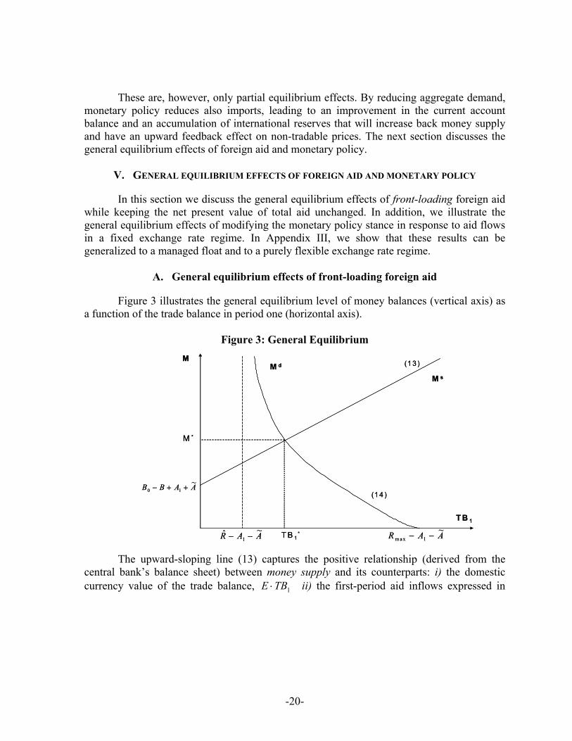
Figure 3 illustrates the general equilibrium level of money balances (vertical axis) as a function of the trade balance in period one (horizontal axis).

Figure 3: General Equilibrium

The upward-sloping line (13) captures the positive relationship (derived from the

central bank’s balance sheet) between money supply and its counterparts: i) the domestic currency value of the trade balance, 1TBE ⋅ ii) the first-period aid inflows expressed in

M s

M d

T B 1*

M *

AABB ~10 ++−

T B 1

M

AAR ~ˆ1 −− AAR ~

1m ax −−

(1 3 )

(1 4 )

M s

M d

T B 1*

M *

AABB ~10 ++−

T B 1

M

AAR ~ˆ1 −− AAR ~

1m ax −−

(1 3 )

(1 4 )

-21-

domestic currency, )~( 1 AAE +⋅ ; and iii) the net domestic assets of the Central Bank BB −0 :20

( ) )~( 101 AAEBBTBEM s +⋅+−+⋅= (13) The downward-sloping curve (14) shows how money demand declines as the trade

balance improves. The intuition is that, for a given income, a higher trade balance in period one is associated with higher savings, smaller consumption, and, therefore, lower money demand:

ATBIATBI

M d

++−

−−

⋅=

1211

1~

11χ (14)

The trade balance needs to be: i) above the threshold AAR ~ˆ1 −− to ensure that the nominal

interest rate remains above the zero lower bound and ii) below the threshold AAR ~1max −− to

ensure that consumption in period one is positive. Appendix I derives equations (13)-(14) and establishes existence and unicity of an equilibrium and that the trade balance must fall within these two thresholds.

Figure 4: Front-loading Consumption Aid without LBD Externalities In the absence of LBD externalities, front-loading consumption aid (i.e., increasing

1A while keeping A constant) shifts period one money supply up. Figure 4 shows that the

20 For notational simplicity, the nominal exchange rate E is assumed to be equal to 1 in the figures.

TB 1

M s

E10

E11

TB11 TB1

0

M

01 >∆A01 <∆TB

M d

TB 1

M s

E10

E11

TB11 TB1

0

M

01 >∆A01 <∆TB

M d

-22-

new equilibrium will be associated with a lower trade balance and higher money balances. Initially, for a given trade balance, the higher money supply puts downward pressure on interest rates and induces agents to increase period one consumption and reduce period two consumption. Higher period one consumption of tradables deteriorates the trade balance and causes a partial reduction of the inital increase in money supply, as shown in Figure 4. As already discussed, this offset is only partial and leaves interest rates below the initial level because part of the higher consumption is spent on nontradables. Given that the trade balance deteriorates less than the initial increase in period one aid, the current account (which includes aid flows) will improve.

In the presence of LBD externalities, the money demand schedule is steeper, hence

front-loading consumption aid has a smaller effect on the trade balance (Figure 5, see the formal proof in Appendix I.A). This happens because, with LBD externalities, an increase in period one aid reduces 2I in equation (14). Given that agents have perfect foresight, they anticipate that a higher aggregate consumption of nontradables in period one will cause a real appreciation of the exchange rate, a shrinking of the export sector, and, in the presence of LBD externalities, smaller productivity, income, and, therefore, consumption in the future. This expectation of lower future consumption will induce agents to save more in period one at the initial level of the interest rate. For a given supply of bonds, these higher savings demand will put downward pressure on interest rates. Therefore, a given level of savings (or trade balance) will be achieved at a lower interest rate, hence at a higher money demand. Figure 5 shows that the same 1A∆ will increase equilibrium money balances more with LBD than without LBD. Figure 5 also shows that 1A∆ has a smaller impact on the trade balance in the presence of LBD, as each individual increases his first period consumption by a smaller amount than without LBD, anticipating lower second period income and consumption. Note, however, that atomistic individuals do not take into account the impact of their own consumption on productivity growth and, therefore savings remains too low from a welfare point of view. 21

21 Note that the definition of externality implies that, while agents predict the effect of the aggregate increase in period one consumption on future productivity, they do not internalize the effects of their individual consumption on future productivity. This inability to coordinate their actions implies that, in the presence of an externality, the decentralized allocation of resources is not optimal from a welfare point of view, and savings are too low. On this point, see the discussion in Section VI.

-23-

Figure 5: Front-loading Consumption Aid with LBD Externalities

In the absence of LBD externalities, front-loading productivity-enhancing aid for

public investment (i.e., increasing A~ by reducing 2A while keeping A constant) shifts money supply up and money demand down (Figure 6). The downward shift in money demand has two components. First, for any given trade balance, the higher productivity (due to a higher A~ ) raises 2I in equation (14) shifting money demand up. The expectation of higher future consumption makes agents try to save less at the initial level of interest rates. For a given supply of bonds, this reduction in savings demand will put upward pressure on interest rates and shift money demand down: a given level of savings will be achieved at higher interest rates, hence at a lower money demand. Second, as shown in equation (14), a higher A~ further reduces money demand at each level of the trade balance. Indeed, since our model assumes that money has no liquidity role for the public sector, the demand for money will fall at any level of the trade balance. Figure 6 shows that, with productivity-enhancing aid, the trade balance will deteriorate more than in the case of consumption aid,22 while money balances will increase if χ is small enough (i.e., the drop in money demand is not too large). The more productive is public investment, the higher is the expected future consumption, and the greater is the deterioration of the trade balance. 22 Note that this result rests on the assumption that spending for investment or consumption have the same composition of tradable and non-tradable goods.

01 <∆ N oL B DT B

01 <∆ L B DT B

M

TB 1

M s

01 >∆ AN o L B D

W ith L B D

M dM d

01 <∆ N oL B DT B

01 <∆ L B DT B

M

TB 1

M s

01 >∆ AN o L B D

W ith L B D

M dM d

-24-

Figure 6: Front-loading Productivity-Enhancing Aid In the presence of LBD, front-loading productivity-enhancing aid for public

investment will result in a somewhat smaller period two productivity benefit. In fact, given that the shares of tradables and non-tradables in the production of the public good are the same as in consumption (equation (8)), A∆ % will raise nontradable prices and reduce the recipient country’s competitiveness, causing at least as much real appreciation as consumption aid and a greater deterioration of the trade balance.23.

Note that the import content of the public good technology has important implications

for whether Dutch disease effects will offset its productivity benefits. For example, if the share of tradable goods used as inputs in the production of the public good is not equal (as we have assumed in Section III.B) but larger than their share in the consumption basket, the Dutch disease effects would be smaller and 2I may increase even for relatively small positive productivity effects of aid. 24 23 This worse trade balance will be associated with a more appreciated real exchange rate in the first period that will make the negative Dutch disease effects on second period productivity larger than in the case of consumption aid.

24 If the direct productivity benefits of A∆ % are large enough to offset its Dutch disease effects, period two income 2I will increase and agents will reduce savings and increase period one consumption. Money demand will then still shift down—albeit by a smaller amount (not shown in Figure 6)―and the trade balance will still be worse than in the case of consumption aid. Conversely, if the direct productivity benefits of A∆ % are not large enough

(continued)

Ms

TB1

E10

E11

TB11 TB1

0

MMd

0~>∆A

01 <∆TB

0~>∆A

Ms

TB1

E10

E11

TB11 TB1

0

MMd

0~>∆A

01 <∆TB

0~>∆A

-25-

The following proposition summarizes the general equilibrium effects of front-

loading aid. Proposition 1 For a constant net present value of total aid: - Increasing period one consumption aid deteriorates the trade balance but improves the

current account and, therefore, raises the stock of international reserves. The larger LBD externalities are, the smaller is the deterioration in the trade balance and the larger is the accumulation of international reserves.

- Increasing period one productivity-enhancing aid leads to a greater deterioration of the trade balance and a smaller accumulation of international reserves. The more productive public investment is, the greater is the deterioration of the trade balance and the smaller is the accumulation of international reserves. The larger LBD externalities are, the smaller is the deterioration in the trade balance.

Proof: see Appendix 1.

B. General equilibrium effects of monetary policy

Figure 7 shows how, in the absence of LBD externalities, sterilization (i.e., a sale of government bonds to the private sector that reduces the central bank’s net domestic assets) can offset the effects of front-loading consumption aid. As interest rates increase to absorb the additional supply of bonds, private agents postpone consumption, nontradable prices fall in relation to tradable prices, and the trade balance improves. In the limit, monetary policy can fully undo the effects of an increase of consumption aid on the trade balance. Similar temporary effects of monetary policy can be found in Edwards (1988) and Calvo et al. (1995), where a temporary depreciation of the real exchange rate is associated with higher real domestic interest rates.

In the presence of LBD externalities, monetary policy can also undo the effects of an

increase of consumption aid. Given that money demand is steeper, the same reduction in net domestic assets leads to a smaller improvement of the trade balance but the latter would have deteriorated less in the first place (see Figure 5).With LBD externalities, however, monetary policy permanently affects the productive structure of the economy. A monetary tightening temporarily depreciates the real exchange rate and leads to an expansion of the export sector, to offset the Dutch disease effects, productivity-enhancing aid will reduce rather than increase period two income 2I and the effects will be similar to those described in Figure 5. Money demand would shift up as long as the upward shift caused by the expected negative LBD effects more than offsets the downward shift due to the lack of a liquidity role for money in the public sector.

-26-

which, in turn, leads to greater LBD and higher productivity in the future. As previously mentioned, Krugman (1987) also argues that monetary policy has permanent effects in the presence of externalities but, in his model, tight monetary policy has opposite effects because he assumes balanced trade and sticky domestic wages.

Figure 7: Sterilization without LBD Externalities

Sterilizing the money supply effects of front-loading productivity-enhancing aid will also reduce period one consumption, improve the trade balance, and raise international reserves and national savings. Central bank’s bond sales would, however, reduce private sector consumption rather than the higher aid-financed public expenditure. With reference to Figure 6, this implies that full sterilization would only shift back the money supply line to its original position while the money demand curve will remain shifted down. Full sterilization would then be able to undo only part of the deterioration in the trade balance, while the current account and international reserves will remain below their initial level.

In the presence of LBD externalities, sterilization raises productivity and future consumption by reducing current private consumption. As a consequence, the Dutch disease effects of an increase in first period aid ( 1A∆ or A∆ % ) diminish. In particular, associating sterilization policy with an increase in aid-financed productivity-enhancing public expenditure A∆ % would maximize the producitivity benefits of aid. These benefits would always need to be traded off against the costs in term of postponed consumption, which could be large if the country is facing a negative output shock.

Proposition 2 summarizes the general equilibrium effects of monetary policy.

T B 1

M s

E 10

E 11

T B 10 T B 1

1

M

0>∆ B

01 >∆T B

M d

T B 1

M s

E 10

E 11

T B 10 T B 1

1

M

0>∆ B

01 >∆T B

M d

-27-

Proposition 2 The deterioration in the trade balance associated with front-loading consumption aid can

be fully offset by a reduction in net domestic assets (“sterilization”) of the same size of the aid increase no matter whether there are or not LBD externalities.

The deterioration in the trade balance associated with front-loading productivity-enhancing aid can only be partially offset by a reduction in net domestic assets (“sterilization”) of the same size of the aid increase. To fully offset the effect on the trade balance, a greater reduction in net domestic assets is necessary.

In the presence of LBD externalities, sterilization raises productivity and future consumption by reducing current consumption.

Proof: see Appendix I.

VI. THE OPTIMAL TIMING OF AID AND MONETARY POLICY

In the previous section, we showed that monetary policy can affect the real exchange rate and the external balance but we have not discussed under which conditions monetary policy can improve (or worsen) welfare, and which factors should be taken into account. To address this question, we proceed in two steps. First, we define the welfare maximization program of a social planner who chooses an optimal distribution of consumption aid over time given the net present value of aid inflows, A . Second, we show that, given an arbitrary distribution of aid over time, agents may or may not achieve the same welfare-maximizing allocation through decentralized equilibrium production and consumption decisions. Agents’ ability to maximize welfare for any given distribution of aid over time depends on: (i) the monetary policy stance, (ii) the existence of LBD externalities; and (iii) external constraints to their borrowing decisions reflecting insufficient international reserves.

A. Social planner’s problem and optimal timing of aid

We assume that both the net present value of aid A and the aid for public investment A~ are exogenously fixed so that the social planner’s problem reduces to choosing optimally

1A and 2A , given a real interest rate equal to the subjective discount rate of the representative agent. The formal maximization program of the social planner is:

( )⎭⎬⎫

⎩⎨⎧

⎟⎠⎞

⎜⎝⎛++=

PMCCWMax AA logloglog 21, 21

χ

subject to: (1) AAAA ~

21 ++= , where A~ and A are exogenous;

-28-

(2) *

2

211

1 1C rPC

Pβ

+= = , where 1≤β is the subjective discount factor of the representative

agent25 and *r is the nominal interest rate that, in equilibrium, determines a real interest rate

equal to 1 1β− .26

Appendix I derives a sufficient condition for a solution to this problem to exist. Our

approach is to solve it by allowing the social planner to choose optimally fictitious aid flows 1F and 2F with AFF =+ 21 such that the current account is balanced in every period (i.e.,

11 TBF −= and 22 TBF −= ). This gives us an optimal consumption (or trade balance) path, characterized by optopt FTB 11 −= and optopt FTB 22 −= , along which donors distribute aid over time so that private sector agents can implement the consumption plan associated with the subjective discount factor β without any need to save or dissave in aggregate because the current account is balanced.

When aid flows are not distributed optimally over time (i.e., optFAA 11

~≠+ and

optFA 22 ≠ ), the same level of welfare could be achieved through accumulation or decumulation of international reserves and corresponding current account deficits and surpluses. Specifically, the welfare-maximizing accumulation of reserves needs to be

optopt FAAR 1`1~−+= with an associated optimal trade balance AARTB optopt ~

11 −−= .

B. Decentralized equilibrium and monetary policy

We now discuss whether, given an arbitrary initial distribution of aid over time, agents can achieve, through a decentralized equilibrium, the optimal reserve accumulation and trade balance. Of course, given that, in our model, monetary policy affects the real interest rate and agents’ decisions depend on it, we also need to characterize the monetary policy stance that would make this optimal decentralized allocation feasible. We characterize

25 In Section III.A, we have for simplicity set 1=β so that agents do not discount the future. In this section, we derive our welfare results for a generic 1≤β , which implies a non-

negative real interest rate (i.e., 2

1

1 PrP

+ ≥ ).

26 As explained in section V, the central bank can target any nominal interest rate r by adjusting its net domestic assets in response to aid flows. Given that monetary policy in our model has real effects, there will be a different real interest rate associated with each nominal interest rate targeted by the central bank.

-29-

such optimal monetary stance with the nominal interest rate optr , which—as we shall see—may be greater or equal than *r depending on whether there are or not LBD externalities.

We denote with *

1TB the trade balance associated with the unconstrained decentralized allocation that agents would achieve if they could borrow and lend at the interest rate *r without limit given their total incomes and aid flows over the two periods. This unconstrained decentralized allocation coincides with the optimal allocation (i.e.,

*1 1

optTB TB= ) in the absence of LBD externalities, while it is associated with overconsumption in period one and it is not optimal (i.e., *

1 1optTB TB< ) in the presence of LBD externalities.

We also denote with 0

1TB the lowest possible period one trade balance that could be financed given the stock of international reserves and period one consumption aid, 1A . There are instances in which the optimal trade balance 1

optTB is not feasible because reserves or first period aid are insufficient. This is the case in which the external financing constraint is binding and 0

1 1optTB TB< . Intuitively, the larger is 1A , the lower is the constrained trade

balance 01TB . This means that front-loading aid (i.e., raising 1A ) can lower 0

1TB up to the point where the optimal allocation can be implemented through a decentralized equilibrium. Proposition 3 - In the absence of LBD externalities, when 0

1TB < optTB1 , monetary policy can make private agents achieve the optimal allocation through an unconstrained decentralized equilibrium (i.e., *

1 1optTB TB= ) by targeting a

nominal interest *r such that, in equilibrium, the real interest rate is equal to 1 1β− .

when 01TB > optTB1 , monetary policy cannot improve welfare, and only front-loading aid can

make agents achieve the optimal allocation. - In the presence of LBD externalities, the unconstrained decentralized allocation always leads to overconsumption (i.e.,

*1 1

optTB TB< ); when 0

1TB < optTB1 , monetary policy can make private agents achieve the optimal allocation through a decentralized equilibrium by targeting an interest rate *optr r> . (Alternatively, donors can back-load aid to induce a binding external constraint so that

* 01 1 1

optTB TB TB< = ). when 0

1TB > optTB1 , monetary policy cannot improve welfare and only front-loading aid can implement the optimal allocation. (However, the external balance constraint must remain binding in equilibrium so that * 0

1 1 1optTB TB TB< = ).

-30-

Proof: see Appendix I.

The key implication of Proposition 3 is that, when aid is not distributed optimally over time, monetary policy needs to be set appropriately to allow agents to achieve an equivalent welfare-maximizing allocation through a decentralized equilibrium. Proposition 3 also indicates that the monetary policy stance needs to be tighter when there are LBD externalities. Finally, Proposition 3 specifies that there are instances in which monetary policy is powerless because of lack of international reserves and where the welfare-maximizing allocation can be achieved only if donors front-load aid. We now describe the intuition underlying Proposition 3 in detail. Timing of aid and monetary policy without LBD externalities

In the absence of LBD externalities, the decentralized equilibrium will be optimal and will be achievable as long as the central bank can target the interest rate *r without making the non-negativity constraint on its international reserves binding.

Consider first the case in which, given the interest rate *r , first period aid is too front-

loaded to maximize welfare. In this case, agents would like to save part of first-period aid to raise future consumption and would increase their demand for government bonds bidding down interest rates. The monetary authority will prevent interest rates from falling by raising the supply of bonds (i.e., reducing net domestic assets), thereby allowing private sector agents to increase their savings and smooth consumption (see section V for a precise description of this mechanism). As private agents reduce consumption, the trade balance will improve and international reserves increase. This increase in international reserves will be a measure of the increase in national savings needed to maximize welfare. Given that, in our model, there is no limit to the reduction in net domestic assets (if necessary they can become negative with the central bank issuing its own bonds) and to the accumulation of international reserves, private sector agents can always achieve the optimal allocation through a decentralized equilibrium, and raise savings in response to an excessive front-loading of aid, as long as the central bank targets the interest rate *r . Note that the required reduction in net domestic assets associated with the excessive front-loading of aid is a form of sterilization that does not require raising the interest rate above *r .

Consider now the case in which, given the interest rate *r , first period aid is too

back-loaded to maximize welfare. In this case, agents would like to borrow against future aid (or income) to raise period one consumption and they would sell government bonds bidding up interest rates. In aggregate, the private sector will be able to dissave only if the monetary authorities buy bonds and prevent interest rates from rising (i.e., they increase net domestic

-31-

assets).27 As private agents increase consumption, the trade balance deteriorates and international reserves fall. In this case, monetary policy cannot achieve any welfare-maximizing allocation. In fact, when the stock of international reserves reaches zero, monetary policy cannot help any longer private sector agents improve on an excessively back-loaded distribution of aid. This happens when the reduction in national savings required to maximize welfare exceeds the stock of international reserves and makes the external balance constraint binding. In this case, it is clear that the only way to maximize welfare is for donors to front-load aid. Timing of aid and monetary policy with LBD externalities

In the presence of LBD externalities, an unconstrained decentralized outcome always leads to over-consumption relative to the optimal allocation because agents fail to coordinate and do not limit their individual consumption enough to reduce the negative externality on future productivity. In this case, to improve welfare, monetary policy can modify the decentralized allocation by raising the interest rate above *r , thereby reducing current consumption and real appreciation.

However, when the decentralized allocation at the interest rate *r makes the external

constraint binding (i.e., * 01 1TB TB< ), monetary policy may or may not be sufficient to

implement the optimal allocation. If the optimal allocation is feasible and the external constraint is binding only because there is overconsumption (i.e., * 0

1 1 1optTB TB TB< < ),

monetary policy can implement the optimal allocation by raising the interest rate to *optr r> . Instead, when the optimal allocation is not feasible because the external constraint would remain binding even after correcting the overconsumption (i.e., * 0

1 1 1optTB TB TB< < ), the only

way to achieve the optimal allocation is to front-load aid and reduce 01TB until it becomes

equal to 1optTB . Note that, however, the external constraint must remain binding in

equilibrium (i.e., * 01 1 1

optTB TB TB< = ).

VII. CONCLUSIONS

This paper points to both opportunities and risks for the conduct of monetary policy in aid-receiving countries. The challenge is twofold: while undoing some of the monetary expansion associated with aid inflows might help smooth consumption over time and contain 27 As discussed in Section II.B, if the private sector does not have any bonds to sell to the central bank, the central bank could implement the same policy through direct monetary financing of the bonds 0B issued by the government. This implies that in our model monetary policy does not face any ceilings on its net domestic assets since 0B can be arbitrarily large. One could have a more complex model in which 0B is constrained.

-32-

Dutch disease, excessive sterilization may stunt current consumption. What is clear is that, in a typical aid-receiving country where aid flows are often disbursed in a haphazard manner and access to capital markets is limited, monetary policy decisions can have a vital bearing not only on nominal magnitudes but also on consumption and productivity growth. We have shown that, when aid flows are excessively front-loaded, monetary policy can improve welfare by increasing gross national savings in the form of higher international reserves. We have also shown that, when aid flows are excessively back-loaded, an expansionary monetary policy can improve welfare provided that the stock of international reserves is large enough.

The idea that there are circumstances in which some aid is better saved owes nothing

to the notion that foreign aid might be too generous. Our results do not provide any indication that an increase in the overall net present value of aid can reduce welfare. They pertain, instead, to the welfare implications of the distribution of a given net present value of aid over time. From this perspective, the declared objective—reiterated at a meeting in Monterrey in March 2002—to raise ODA to 0.7 percent of industrial countries’ GDP from a level that is currently only about one third of that target can only be welcome.28 Monetary policy should, however, take into account whether industrial countries are likely to sustain their commitment over time and make this surge in aid permanent. The focus of this paper on the distribution of aid over time makes it, instead, highly relevant for assessing the welfare and monetary policy implications of initiatives such as the International Financial Facility proposed by the United Kingdom that the international community is currently debating and that aim at bringing aid forward to achieve the MDGs by 2015.

While the theoretical arguments for welfare-improving monetary policy intervention are compelling, some perspective is in order. First, there are remarkably few empirical studies of Dutch disease in aid-receiving countries. If LBD spillovers are quantitatively insignificant, monetary policy will have negligible permanent effects on real variables. Nevertheless, as long as capital market access of aid-receiving countries remains limited, monetary policy will retain an important consumption smoothing role. Second, information requirements for designing a welfare-improving monetary policy appear staggering. Choosing the appropriate monetary policy stance requires factoring in a multitude of elements, ranging from the benefits of higher current consumption to determinants of aid effectiveness and productivity growth such as the quality of institutions, corruption, and capacity constraints. A reliable forecast of future aid inflows is, of course, another critical input to monetary policy formulation. Nonetheless, our paper shows that these are essential inputs to the policy-making process and cannot be ignored.

28 Tripling ODA is viewed as a necessary step to achieve the Millennium Development Goals by 2015 (Heller and Gupta, 2002). The Millennium Development Goals (MDGs), which emerged from the September 2000 Millennium Declaration at the United Nations, are a set of measurable targets for halving world poverty between 1990 and 2015.

-33-

Actual monetary policy decisions should also focus on aspects of sterilization policy that we do not consider. In our stylized model, sterilization is effective because bond sales reduce consumption. In practice, however, sterilization is also implemented through fiscal surpluses that reduce government deposits at the central bank. If fiscal surpluses are achieved by postponing the very public investment that is supposed to be financed with the aid increase (as opposed to reducing current expenditure), the trade balance and Dutch disease effects of aid would be undone but any related productivity benefit would be lost as well. Our model also abstracts from possible sterilization costs associated to bond issuance.29 These costs cannot be overlooked in practice. If the taxes needed to finance the differential between the interest rates on sterilization bonds and international reserves are distortionary or costly to be levied, sterilization would have welfare costs that should be weighed against the benefits of smaller Dutch disease effects. These costs would, of course, be even larger if high interest rates depressed interest-sensitive private investment that might enhance productivity.

This paper also points to some important limits to managing aid inflows with

monetary policy, such as insufficient levels of international reserves. Faced with these limits, donors could demonstrate a newfound resolve and decide to coordinate their actions, minimize aid volatility, and, thereby, reduce the need for monetary policy intervention. There is little doubt that better planning in disbursing aid flows would go a long way towards improving welfare of recipient countries. Pallage and Robe (2003) show that reducing the volatility of consumption in developing countries would yield substantial gains.30 Increasing multilateral and bilateral donors’ coordination in disbursing aid—a key objective of the PRSP process introduced in the late 1990s—is then essential.

Allowing recipient countries to save directly aid for later use is an alternative to be

considered if greater coordination of donor countries turns out to be an unrealistic objective. Donors could set up country-specific reserve funds in which aid is accumulated and then spent when aid flows or other resources dry up. The key challenge would, however, be the governance of such funds, which requires resolving the tension between predictable and timely assistance on the one hand and donors’ desire to subject the use of the fund’s resources to conditionality on the other. Indeed, for aid-receiving countries, accumulating international reserves is an appealing alternative as it allows them to save aid in a form that involves little or no conditionality. Nonetheless, given that sterilization policy may be costly, further work could be devoted to designing a governance structure that might make aid reserve funds feasible.

29 As discussed in Section III.C, sterilization costs could be easily introduced in our model without changing the qualitative features of our results.

30 Pallage and Robe (2003) estimate the median welfare cost of business cycles in developing countries to be between 10 and 30 times that of the United States.

-34-

APPENDIX I

A. Solution strategy

The static analysis of this model is standard. The static equilibrium relation between the real exchange rate and the allocation of labor in each period is the outcome of equilibrium conditions on the labor market and non-tradable goods markets. First, perfect mobility of labor implies that the marginal productivity of labor is the same in the tradable and non-tradable goods markets:

( ) ( )tNNtNtNtNXtXtXt LFapLLFapw ,,,,,, ′⋅⋅=−′⋅⋅= , t=1,2.

Hence:

′

′⋅=

N

X

tN

tXtt

F

Faa

qe,

,

, t=1,2. (A-1) Second, equilibrium on the non traded-goods market implies that:

( )( )⎩⎨⎧

=−

=+−

2,2,22

1,1,1,1,11

11

NN

NNNN

ypCPypxpCP

γγ

Combining these conditions with the aggregate budget constraints, we obtain the two following equilibrium relations: Period 1:

( )[ ] ( ) ( ) ( )( ) ⎥

⎥⎦

⎤

⎢⎢⎣

⎡ −+−⋅⋅−=−⋅⋅ *1

`11111111 1T

NXXNNNNp

RALLFaqxLFae γγ (A-2a)

Period 2:

( ) ( ) ( ) ( )( ) ⎥

⎥⎦

⎤

⎢⎢⎣

⎡ ++−⋅⋅−=⋅⋅ *

2,

`22,2,12,2,

2 1T

NXXNNN pRALLFaqLFae γγ

(A-2b) The demand for real money balances is the following:

⎟⎠⎞

⎜⎝⎛ +=

rCP

M 11111

χ (A-3) By substituting (11-1) and (11-2) into the aggregate private sector constraint, we obtain the following economy-wide resource constraints:

1111 AIRCP +=+ (A-4a)

RAICP ++= 2222 (A-4b) Therefore, in this economy with a closed capital account and no accumulated factor of production,

national savings are simply reflected in the accumulation of foreign currency by the central bank and by individuals. Monetary policy affects the inter-temporal allocation of resources insofar as it has a (temporary) effect on the current account balance by reducing (or increasing) aggregate demand. As discussed in Section III.C, this happens because changes in money supply affect both nominal and real interest rates and, in turn, private savings decisions through the inter-temporal consumption smoothing condition:

1

2

12 /1

CC

PPr

=+

(A-5)

-35-

In sum, we have 15 unknown variables: the real exchange rates 1e and 2e , the equilibrium allocation

of labor between non-tradable and tradable production 1,NL and 2,NL

, the CPI levels 1P and 2P , the

aggregate consumption indices 1C and 2C , the nominal interest rate r , the nominal value of domestic

currency 1M and foreign currency *1M , the face value of bonds B held by the private agents, the reserves R

accumulated during period 1, and the allocation of aid for productive purposes A~ between non-tradable Nx

and tradable goods Tx . We have 14 equations: the equilibrium on the non-traded good market, the demand for labor in traded and non-traded sectors, the definition of the consumer price index, the aggregate resource constraints, the demand for domestic bonds, the demand for real money balances, the money supply identity, the balanced budget equation and the production technology of the public good.

Thus, the government can use monetary policy (the face value of bonds B sold to private agents, or the nominal interest rate r) to affect macroeconomic outcomes by targeting the current account via the accumulation of reserves.

Finally the real consumption indexes are given by:

⎪⎪

⎩

⎪⎪

⎨

⎧

⎥⎥⎦

⎤

⎢⎢⎣

⎡

⋅+

+⋅+⋅=

⎥⎥⎦

⎤

⎢⎢⎣

⎡

⋅−

+⋅+⋅=

*2,2

22,

2

22,22

*1,1

11,

1

11,11

TXN

TXN

peRAy

eqyeC

peRAy

eqyeC

γ

γ

B. Proofs of Propositions

Existence and Unicity of Equilibrium To keep notations simple, we assume that 0~

=A . One can easily check that the result holds for 0~≠A .

First, we show that if an equilibrium exists, it is unique. Second, we establish existence of an equilibrium. Unicity of equilibrium Unicity is established in the following way.

First, if an equilibriun exists, aggregate intertemporal decisions are characterized by the current account balance in the first period (or equivalently the accumulation of reserves R between period one and period two).

Second, we simply remark that for each current account balance R in the first period there exists a unique equilibrium of the real economy characterized by real exchange rates ( )Re1 and ( )Re2 , price levels

)(1 RP and )(2 RP (recall price levels are pinned down by equations (1-1) and (1-2)), consumptions ( )RC1

and ( )RC2 and allocation of labor between the export and non-tradable sectors ( )RLN 1, and ( )RLN 2, . In

other words, there exists a unique correspondence between a level of reserves R and the equilibrium of the economy with an exogenous current account equal to R . Indeed, the real side of the model is a standard Dutch disease model with a learning by doing externality, as in Van Wijnbergen (1984), Krugman (1987), Matsuyama (1992), Sachs and Warner (1995), Gylfason et al. (1997), Torvik (2001), and Matsen and Torvik (2004) among others.

-36-

Finally, the accumulation of reserves R is pinned down by the money market equilibrium as shown on Figure 3. Since the sM and dM locus are well-behaved curves (just note that first period nominal consumption is a decreasing function of R, while second period consumption is increasing with R), there is at most one level of reserves R that guarantees equilibrium on the money market.

Existence of Equilibrium To establish existence, we must show that the sM and dM locus on Figure 3 have a non-empty intersection. Necessary conditions comes from the dM locus. Recall that it is derived by combining the money demand (A-3) and the intertemporal consumption smoothing equation:

2211

111

CPCP

M d

−⋅= χ

Therefore a necessary condition for existence of an equilibrium is: 2211 CPCP < , which translates into a constraint on the admissible equilibrium current accounts (or reserves R ).

Indeed 2211 CPCP < is equivalent to: ⎟⎠⎞

⎜⎝⎛ +−+> 2

21

12 AEIA

EIR

Assuming for simplicity that the international price of the import good is constant ( **2,

*1, TTT ppp == ), and

using equations derived in Appendix I.A, the condition becomes: ( )22,22,211,11,12 AyeyqAyeyqR NXNX +⋅+⋅−+⋅+⋅>

The right hand side can be interpreted a a function of R , computed at the equilibrium of the economy with an exogenous current account equal to R .

Define ( ) ⎟⎠⎞

⎜⎝⎛ +−+= 2

21

1 AEIA

EIRG .

dRdI

dRdI

dRdG 21 += and:

{ Re

eI

RL

LI

RI

dRdI i

i

iiN

iN

iii

∂∂⋅

∂∂

+∂

∂⋅

∂∂

+∂∂

=

==

,

0

,0 321

, for i=1,2.

Indeed, ( ) ( ) 0,'

,,,'

,,,

=⋅⋅+−⋅⋅−=∂∂

tNNtNtNtNXtXtXtN

t LFapLLFapLI

for t=1,2 in the neighborhoods

of the labor market equilibrium for an exogenously set current account.

Moreover, ( ) tNtTt

t ypeI

,*

, ⋅=∂∂

, for t=1,2.

Hence { {

0

0

22,

*2,

0

11,

*1, <

∂∂⋅⋅−

∂∂⋅⋅=

><

Reyp

Reyp

dRdG

NTNT

This implies that for each combinations of parameters, there exists a minimum current account surplus (accumulation of reserves) [ [max,0ˆ RR∈ above which an equilibrium always exists, with

-37-

R̂ defined by the implicit function: ( ) ( )

RAERIRA

ERI ˆ

ˆˆ

ˆ2

21

1 ++=−+ if ( ) 00 >G , and: 0ˆ =R

if ( ) 00 ≤G ,

and maxR defined by the implicit function: ( ) 0max11 =RCP , or:( )

01max1

max >+= AERI

R .

Since the function G is an increasing function of the degree of frontloading of foreign aid ( 21 AA − ), this also

implies that R̂ increases with 21 AA − , but by less than 21 AA − (see figure below), which implies that the corresponding trade balance must deteriorate. It is easy to see that the set of possible current account equilibria is non-empty. These claims can be visualized on the following figure (it is here assumed that ( ) 00 >G ):

These necessary conditions themselves do not guarantee existence. A look at Figure 3 shows that an additional condition must hold to guarantee existence of an equilibrium: ( ) ( )00 =≥= RMRM sd . Together with the two constraints on R, it is sufficient to establish existence of an equilibrium. This condition is equivalent to:

gAIBB

AIAI

AIBB

⋅+−

=⎥⎦

⎤⎢⎣

⎡−

++

⋅+−

≥22

0

21

22

22

0 1χ where g is the growth rate of income including aid between

period 1 and 2. Hence,this translates into a condition on the net domestic assets of the Central Bank and the growth rate of the economy.. For instance, if the growth rate is 5 percent, and the net domestic assets of he Central Bank are worth 20 percent of GDP, this implies that 001.0≥χ , which is small enough to be reasonable.. Proof of Propositions 1 & 2: Real and Monetary Effects of Aid Inflows and Monetary Policy Let us express the current account balance R as the sum of the trade balance in the first period and first period aid: AATBR ~

11 ++= , and 22 ATBR −−= .

This im,plies that ATBAAATBTB +=+++=− 12112~

or: ( ) AAAATBTB =++=+−~

2112 so the present value of the trade deficit is equal to the present value of aid inflows.

4 5 d e g r e e l i n e2 R

A 1 - A 2 i n c r e a s e s

R

G ( R )

R m a xR

S e t o f p o s s ib le e q u il ib r iu m c u r re n t a c c o u n t b a la n c e s

4 5 d e g r e e l i n e2 R

A 1 - A 2 i n c r e a s e s

R

G ( R )

R m a xR

S e t o f p o s s ib le e q u il ib r iu m c u r re n t a c c o u n t b a la n c e s

-38-

Thus, tthe money demand equilibrium locus dM and money supply sM are functions of the trade balance and aid inflow in the first period:

( ) ( )

⎪⎪⎩

⎪⎪⎨

⎧

++−

−−

⋅=

+++−=

ATBIATBI

M

AATBBBM

d

s

1211

110

1~

11χ (13 & 14)

The locus dM is the equilibrium relation between income, the external balance and the money demand. Hence income and trade balance are those resulting of a given aid inflow and consistent with a given money supply equal to dM . It is straightforward to check that the locus dM is a decreasing function of the trade balance in the first period. We characterize the effects on the money market and the external balance of an increase in first period aid flows (consumption aid or aid for public investment) realized by lowering second period consumption aid, for a given net present value of total aid flows A . Impact of increased aid flows / monetary policy in absence of externalities The impact of an increase in first period aid A1, holding the total amount of aid A and the supply of public bonds to the private sector constant, is as follows, and is described on Figure 4 in the main text. The increase in first period consumption aid is obtained by lowering second period aid. This implies that A~ and A are fixed and that the externality associated with the public good can be assumed away and ( )Pxh is simply a parameter.

At the initial equilibrium is 01E money supply initially shifts up by the amount of the aid inflow, for a given

trade balance. Hence, at the initial trade balance, the money supply exceed the money demand, putting downward pressures on interest rates since the supply of bonds remains constant. Agent will reduce their savings and increase their demand for money. Simultaneously, agents will increase their consumption after receiving the aid inflow 1A , for a given income 1I , leading to a deterioration of the trade balance in the first period. This deterioration in the trade balance and the increase in money demand due to higher consumption and lower interest rates appears as a shift to the left along the locus dM . The new first period equilibrium will be at 1

1E . Since the money supply curve shifts up by 1A exactly, it is easy to see that the deterioration of the trade balance will be smaller in absolute terms than the increase in first period aid. This happens because par t of the aid received is spent on non-tradable goods. Thus, the equilibrium current account (including aid) will improve by less than the increase in first period aid. Let us now consider an increase in aid for public investment A~ (see Figure 5 in the main text). In this case. the money demand curve will also shift down. Indeed, a larger share of the trade balance will be generated by the public investment, and as money has no liquidity role for the public sector, a given trade balance will be consistent with a smaller money demand. Indeed, if the trade balance remains unchanged, a larger share of first period private income must be saved, which depresses the money demand. As a consequence, no money demand effect that partly offsets the impact of the money supply expansion on the trade balance will be smaller, and the deterioration of the trade balance will be larger. A second mechanism will reinforce this effect. Indeed, as A~ increases productivity in the second period, 2I willbe directly affected by A~ . A positive productivity effect implies that the money demand will have to shift even further down to maintain a given trade balance (as agents will be willing to spend even more in the first period if they expect a higher second period income). In other words, a higher interest rate will be needed to support a given level of savings (or trade balance). For small values of χ , the money supply effect will dominate the demand effect, and money will increase in equilibrium.

-39-

Summary: This discussion shows that under the assumptions of the model, the same increase in aid will have

different implications for the external balance if it is spent on public investment instead of private consumption. The deterioration of the trade balance will be greater in the former case. It will be even greater the more productive foreign aid is. Impact of changes in the monetary policy stance: The impact of a reduction in the net domestic assets of the Central Bank (sterilization) is simply the opposite shift in the money supply curve without any shift in the money demand curve. It is easy to see that it would lead to a new equilibrium with an improved current account and higher interest rate (Section V.B). Impact of Dutch disease externalities Let’s consider the impact of an increase in consumption aid in the first period realized by lowering second period aid, in presence of Dutch disease externalities. With LBD, the money demand schedule is steeper.

To see why, note that the LBD externality implies that ⎟⎟⎠

⎞⎜⎜⎝

⎛+=−=

+)(

1122~ATBARII : an improvement in the

equilibrium current account net of the aid flow (hence a lower aggregate consumption in the first period) is associated with a lower consumption of the non-traded good in the first period, a larger traded sector, and a higher productivity gain in the second period. Another way to see this is to remark that a lower aggregate consumption in the first period leads to higher productivity growth, and that first period consumption is increasing with aid flows net of reserves: RA −1 . With perfect foresight, agents anticipate this productivity effect for a given aggregate consumption, hence they will reduce their own consumption in the first period, lowering money demand. However, ,atomistic agents do not internalize the effect of their own consumption pattern on productivity,and savings will remain to low from a welfare point of view. Since AARTB ~

11 −−= , this implies that the money demand in the money-trade balance space schedule will be steeper. This property of the money demand can be formalized as follows from equation (14). For any trade balance 1TB , the slope of the money demand schedule is given by:

01

2

2

22

1

22

221

11

111 11

<⎥⎥⎥

⎦

⎤

⎢⎢⎢

⎣

⎡

∂∂

⋅∂∂

+∂∂

⋅∂∂

+∂∂⋅

∂∂

=

+++−−+

= 321321321321321321TBI

ICP

TBCP

CPM

TBCP

CPM

dTBdM dd

TBTB

d

Moreover, 01

2 =∂∂TBI

if 0=z and 01

2 >⎟⎟⎠

⎞⎜⎜⎝

⎛∂∂TBI

dzd

. Since the other terms of the derivative do not depend

on z , it must be clear that 01

<⎟⎟⎠

⎞⎜⎜⎝

⎛dTBdM

dzd d

.

The following results follow from this property of the money demand schedule: - an increase in first period aid leads to a smaller deterioration of the trade balance the larger the LBD

externality ; - symmetrically, a given reduction in the net domestic assets of the Central Bank leads to a smaller

improvement of the trade balance the larger the LBD externality is. Proposition 3: The Optimal Allocation of Aid The proof proceeds along the following steps. First, we define the welfare maximization problem of a social planner.

-40-

Second, we derive constraints on the trade balance in the decentralized equilibrium. Third, we compare the decentralized equilibrium for a given distribution of aid flows to the optimal consumption path chosen by a social planner, and discuss under which conditions a reallocation of aid flows or monetary policy can improve welfare. In the following, we assume that A~ is exogenous, and focus on the time allocation of consumption aid, for a given total net present value of aid flows. Welfare maximization problem: The social planner chooses the time allocation of aid maximizes the intertemporal utility function of the representative agent under the following constraints: (1) the total net present value of aid and aid for public investment are set exogenously;

(2) the interest rate is equal to the rate of time preference of agents: 111

22* −==CPCPrr , where 11* −=

βr

( 1<β ) is the subjective discount rate of the representative agent (we have so far assumed that 1=β ).

Formally, for a given net present value of aid A , the donor objective is to choose a time allocation of consumption, or equivalently a trade balance AARTB ~

11 −−= , to maximize:

⎭⎬⎫

⎩⎨⎧

⎟⎟⎠

⎞⎜⎜⎝

⎛+

++=

12*1 loglog

11log

1 PMC

rCWMaxTB χ where: ⎟

⎠⎞

⎜⎝⎛ +⋅= *1

1

11r

CPM χ is the demand for

money , 1C and 2C are the consumption indexes, and productivity parameters depend on the equilibrium trade

balance: )~( 1222 AARaaa XN −−==

Thus the maximization problem simplifies to:

( )⎭⎬⎫

⎩⎨⎧

⎟⎟⎠

⎞⎜⎜⎝

⎛⎟⎠⎞

⎜⎝⎛ ++

++⋅+= *2*1

11loglog1

1log11 r

Cr

CWMaxTB χχχ

Hence, one simply needs to derive the optimal saving plan for an economy in which the rate of time preference

is ( ) ( )χβ+⋅+

=11

1*r

. Given the aggregate budget constraints and the definition of the trade balance in

each period, this is equivalent to deriving the optimal time allocation of fictitious aid flows 1F and 2F in an

economy with balanced current account, where RAAF −+=~

11 and RAF += 22 . Indeed, this

transformation keeps the total net present value of aid flows unchanged: AFF =+ 21 .

The solution to this problem provides the optimal accumulation of reserves optopt FAAR 1`1~−+= and trade

balance AARTB optopt ~11 −−= in the first period for an economy in which we do not impose a balanced

current account. These variables can next be compared to the decentralized equilibrium. The detailed proof is as follows. The derivative of the welfare function with respect to 1F and 2F can be decomposed in the following way:

1

1

1

1,

2,2,1

1

1

1,

1,1

1

111 Fe

eL

aW

aWZ

Fe

eL

LW

Fe

eW

FW

dFdW N

Nx

N

N ∂∂⋅

∂

∂⋅

⎥⎥⎦

⎤

⎢⎢⎣

⎡

∂∂

+∂∂

⋅−∂∂⋅

∂

∂⋅

∂∂

+∂∂⋅

∂∂

+∂∂

=

where ( )( )AxhzLa

La

Z PN

N

N

X ~

1,

2,

1,

2, ⋅=∂

∂−=

∂

∂−= ,

-41-

and: 2

2

2

2,

2,2

2

222 Fe

eL

LW

Fe

eW

FW

dFdW N

N ∂∂⋅

∂

∂⋅

∂∂

+∂∂⋅

∂∂

+∂∂

= .

Note that:

(1) 0,,

=∂∂⋅

∂∂

=∂∂

ttN

t

tN IW

LI

LW

, t=1,2, in equilibrium:

Indeed, from the firms’ profit maximization conditions: 0,

,,

,

,,

,

=∂

∂⋅−

∂

∂⋅=

∂∂

tX

tXtX

tN

tNtN

tN

t

Ly

pLy

pLI

.

(2) 0=∂∂

t

t

eC

, t=1,2.

Indeed :

( ) ( )

011

11

,,,,

*1,

12

11,2

1

11*

1,

1

11,1,

1

111

=⋅=−⋅−⋅

=

⎥⎥⎦

⎤

⎢⎢⎣

⎡+⋅⋅−

⎥⎥⎦

⎤

⎢⎢⎣

⎡⋅++⋅⋅=

∂∂ −

t

t

tt

tttXtXtTtT

t

TX

TNX

t

t

PCA

ePFEypcp

e

pF

ey

eqe

pF

eyy

eqe

eC γγγ

(3) 02

2

22

=∂∂⋅

∂∂

=∂∂

eC

CW

eW

(4) 01

1

11

=∂∂⋅

∂∂

=∂∂

eC

CW

eW

(5) Simple algebra yield:

ttt

t

tt FIFC

CW

FW

+=

∂∂⋅

∂∂

=∂∂

*

1, t=1,2, with:

t

tt E

II =* .

And:

222

2

22,2,

1FEI

Iaa

WaW

NX +⋅=

∂∂

+∂∂

.

Therefore the marginal benefit (MB) and marginal cost (MC) of increasing 1F are respectively:

1*1

11)(

FIFMB

+=

( )1

1

1

1,

22*2

*2

2*2

11

Fe

eL

haz

FII

FIFMC N

∂∂

∂

∂⋅⋅

++

+= where 12 FAF −=

A sufficient condition for the MC curve to be downward sloping is 2a

zhsmall, which is equivalent to:

1,1

1 XzLaz

+<< . A sufficient condition is therefore: 11

<<az

Indeed, ( )1

2

21

11'

FI

IMC

FMC

FMC∂∂⋅

∂∂

+∂∂

=

-42-

Where: ( ) ( ) ⎟⎟

⎠

⎞⎜⎜⎝

⎛∂

∂

∂∂

⋅⋅⋅+

+∂

∂⋅⋅⋅

++

+=

∂∂

1

1,

1222

2

1

1,

22

22

22

221

1 1F

LF

haz

FII

FL

haz

FII

FIFMC NN

Combining (A-1) and (A-2), the amount of labor allocated to the non-traded sector in period 1 is solution to the following, assuming again that ttXtN aaa == ,, , t=1,2:

1,11,

1,

1

1,

1, *11

N

pF

N

N

N

N

LaLLL

qLL

Lq T

γγγ

αα

+⎟⎟⎠

⎞⎜⎜⎝

⎛ −⋅⋅⎟⎟

⎠

⎞⎜⎜⎝

⎛ −=⎟

⎟⎠

⎞⎜⎜⎝

⎛

−

−

which gives an implicit function: ( ) 0, 11, =FLH N

Hence, ( ) ⎟

⎟⎟

⎠

⎞

⎜⎜⎜

⎝

⎛

∂∂

∂∂

∂∂

−=∂

∂

N

N

LH

FH

FFL 1

12

1

12

. One can show that: ( ) ( )

012

1

2*

21

12

>⋅=∂

∂

NN

TN

LLa

pFL

αγ

α

Next 01

2 <∂∂FI

in presence of LDB externality, while ( ) ( ) 1

1,2

22

2

222

1F

Lazh

FIF

FIIMC N

∂

∂

++

+−

=∂∂

Therefore a sufficient condition for 2I

MC∂∂

to be positive is again that 2a

zhis small and

1

1,

FLN

∂

∂not too large,

which is the case as long as the non-traded sector is large enough.

Indeed, one can show that: ( )NNN

TN LZLap

FL

⋅=∂

∂αγ

*

1

1,

1.

Constraints on the trade balance Before characterizing the constraints on the trade balance in this model, let us note that the time path of aid does not always matter in the decentralized equilibrium despite the fact that the capital account is closed. Indeed, as long as the Central Bank holds enough reserves initially, agents can reduce their holdings of public bonds (this reducing their savings), and increase their consumption. In fact, since there are no ceiling on the issuance of public bonds 0B and that the income generated by the issuance of bonds is always redistributed to agents, there is no ceilings on the net domestic assets of the Central Bank even if the amount of bonds held by the private agents B is never negative. This implies that monetary policy can be arbitrarily expansionary as long as the external balance constraint is met. Since an expansionary monetary policy implies greater private consumption, the decentralized equilibrium mimicks the one of an economy with perfect capital market as long as the constraint on international reserves is not binding. In fact, the equilibrium aggregate international reserves play the role of the storage technology allowing consumption smoothing. The macroeconomic analogy with an economy with perfect capital markets is clear from the economy-wide budget constraints:

⎪⎩

⎪⎨⎧

++=

−++=++

RAICPRAAIxpxpCP NNTT

2222

111,1,1,1,11~

with 12~ AAAA −−= and Axpxp NNTT

~1,1,1,1, =+

However, if the Central Bank has limited reserves 0R , and first period revenues are low relative to second

period revenues, the constraint 0RR ≤− on the external balance will be binding, and the distribution of aid

will matter. Let us consider an economy in which 00 =R . The trade balance for which the external balance’ constraint is binding is the following

AATB ~11 −−=

-43-

indeed AATBR ~0 11 −−=⇔= .

Thus, it is a decreasing function of first period aid. The constraint RR ˆ> must also be met. Using the definition of R̂ and the trade balance, one obtains the following condition on the trade balance:

( ) ( )( )⎟⎠⎞

⎜⎝⎛ −−−−⋅−−> 21211111

~21,~max ATBIAATBIAATB . From the proof of the existence of

equilibrium, it is easy to see that the RHS of this inequality is a decreasing function of first period aid. So, the constraint on the trade balance to have an interior decentralized equilibrium is:

011 TBTB > where 0

1TB is defined by the implicit function:

( ) ( )( )⎟⎠⎞

⎜⎝⎛ −−−−⋅−−= 2

0121

0111

01

~21,~max ATBIAATBIAATB

Moreover, in the economy in which *rr ≈ , the limit lower bound for the equilibrium trade balance to have a well defined money demand is given by 2211 CPCP = , or AARBT ~ˆˆ

11 −−= . Therefore, using the

definition of R̂ one can show that: ( ) ( ) ( ) 111~2ˆ

1011 −+⋅+≤+⇔≤ agaaTBBT

where g is the growth rate of nominal GDP between period 1 and period 2,

and 1

11 I

Aa = ,

1

~~

IAa = , and

2IAa = .

Decentralized Outcome versus Optimal Outcome: the Role of Redistributing Aid Define *

1TB the equilibrium trade balance of an economy in which the Central Bank has unlimited initial reserves. Hence, a corner equilibrium is more likely to happen ( 0

1*1 TBTB < ) when (1) total aid flows are large relative

to GDP, (2) GDP is expected to grow at a high rate, and (3) aid flows are backloaded. In such a situation, it is clear that the allocation of aid will affect consumption patterns and welfare. Consider first the case in which there is no LDB and h=0. In such a case, optTBTB 1

*1 = .

In this case, holding other parameters constant, an increase in 1A will increase first period consumption, and

improve welfare as long as 01

*1 TBTB < . Conversely, a further increase in 1A won’t affect consumption and

welfare if optTBTB 1*1 ≥ , i.e. when 2A becomes small.

For the same reason, for a given allocation of aid, a negative shock on first period income, holding future growth prospects constant, will make front-loading aid more likely to improve welfare. Next, in presence of LDB and with h=0, optTBTB 1

*1 < , i.e. agents do not internalize the impact of their first

period consumption decision on LDB (However, they do anticipate a lower income if aggregate first period consumption rises, as already discussed). Three cases arise: (1) 0

11*1 TBTBTB opt << . It is then optimal to increase first period aid, but by less than in the previous

situation, until 011 TBTBopt = ,(i.e. the external balance constraint is still binding in equilibrium: 0

1*1 TBTB < )

which is the optimal allocation of consumption between period 1 and period 2.

-44-

(2) optTBTBTB 101

*1 << : even though agents are constrained in their consumption decisions, and the Central

Bank does not accumulate any reserves between period 1 and period 2, it is optimal to decrease first period aid until optTBTB 1

01 = . In other words, it is optimal to make the external balance more constrained.

(3) optTBTBTB 1*1

01 << : in this case the economy is not constrained, but it is optimal to make it constrained

by reducing first period aid until: optTBTBTB 101

*1 =< .

An alternative to back-loading aid in cases (2) and (3) is for the Central Bank to raise the interest rate above *r to induce a higher saving rate by private agents.

Finally, it is easy to see that in presence of LDB and with 0≠h , the desired decentralized equilibrium trade balance *

1TB can be either above or below the one for which there is no LDB and h=0, depending on the relative size of the two effects. However, agents will always overconsume in the first period, hence the following inequality will still hold optTBTB 1

*1 < .

-45-

APPENDIX II. MANAGED FLOAT AND FLEXIBLE EXCHANGE RATE REGIMES In this section, we show that our results on the role of monetary policy can be generalized to countries

with a managed float or with a flexible exchange rate regime.

Managed Float

In the case of managed float, the equilibrium real exchange rate adjusts to any given monetary policy and intervention policy through the nominal exchange rate instead of the price level. The CPI levels 1P and 2P are the nominal anchors (price level targets) for monetary policy, and the central bank chooses an intervention policy in the foreign exchange market that targets a level of foreign exchange reserves 0RR = . The nominal and the real exchange rates adjust to a level consistent with the price and reserve targets.

Formally, the nominal exchange rates in each period are derived from the current account constraints. In the first period the equilibrium nominal exchange rate 1E equates the supply (exports revenues and aid

inflows) and demand of foreign currency (imports, reserves bought by the central bank 0R , and foreign currency held by private agents). In the second period, the supply of foreign currency is the sum of reserves held by the Central Bank, foreign currency held by domestic agents, exports revenues and foreign aid inflows; the demand for foreign currency is simply the demand for imports:

( ) ( ) ( )( ) ( )⎪⎩

⎪⎨⎧

=+++

++⋅=⋅+⋅++

2,*

2,22,*

2,*10

11,*

1,1,*

1,1,*

1,*10

~

TTXX

XXTTTT

cpAypMR

AAypxpcpMR

The central bank chooses net domestic assets BB −0 to generate a level of aggregate demand consistent with the targeted price levels and international reserves.

The central bank can implement the same allocation of resources of the case with fixed exchange rates. Consider, for instance, an equilibrium with reserves *R , price levels *

1P and *2P , and bonds held by the

private sector *B that are consistent with fixed exchange rates *1E and *

2E . Note that the price levels *1P and

*2P and the nominal exchange rates *

1E and *2E uniquely characterize the equilibrium real exchange rates

*1e and *

2e (see equations (1-1) and (1-2)), which, together with international reserves *R , determine the allocation of resources and consumption-savings decisions. This resource allocation can be replicated with price

targets *1P and *

2P exogenously set, a target for international reserves *0 RR = , and net domestic assets

BB −0 such that the private sector holds *B . These policies would imply different price levels *1P and *

2P

and nominal exchange rates *1E and *

2E than in the fixed exchange rate regime case but the same real exchange rates:

⎟⎟

⎠

⎞

⎜⎜

⎝

⎛

⋅

−

=*

1,*1

*1

11

*1

T

e

pE

Pγ and

⎟⎟

⎠

⎞

⎜⎜

⎝

⎛

⋅

−

=*

2,*2

*2

11

*2

T

epE

Pγ

-46-

Floating exchange rate

In principle, in a country with a purely floating exchange rate, the central bank does not intervene in the foreign exchange market, and therefore does not accumulate foreign exchange reserves. This seems a priori to rule out the extension of our model to the case of a pure float.

In reality, however, even in floating exchange rate regimes, aid-receiving governments do not

exchange foreign currency for domestic currency on the foreign exchange market, as discussed in Section II.C. Instead, they tend to deposit their foreign-currency aid at the central bank. Initially, this operation raises international reserves and reduces net domestic assets by the same amount. When the government starts drawing on its account at the central bank to finance public expenditure or transfers, money supply grows. The central bank can then undo this monetary expansion through open market sales of bonds or the government can postpone drawing down its account to allow the central bank to achieve its net domestic asset target BB −0 .31 The central bank may also need to conduct a one-off intervention in the foreign exchange market to bring international reserves in line with the targeted current account and gross national savings.

In a pure float, if the government holds deposits with commercial banks rather than at the central bank, foreign aid inflows will not automatically increase base money. To our knowledge, however, the only case among aid-receiving countries of governments holding deposits with commercial banks is that of CFA African countries. Given that these countries have a fixed exchange rate regime, base money still increases in response to aid inflows because commercial banks request domestic currency in exchange of foreign currency when the government needs to spend the aid deposited with them.

In practice, the case of a flexible exchange rate can be seen as equivalent to the case of a managed float. On the domestic side, monetary expansion does occur as a result of government deposits at the central bank while sterilization policy remains feasible. On the external side, foreign exchange intervention is a one-off action limited to periods of foreign aid inflows, and can be used to target a desired level of foreign exchange reserves

31 Such fiscal sterilization of foreign aid inflows was used for instance in Mozambique (see Buffie et al. 2004).

-47-

REFERENCES [1] Acemoglu, D., Johnson, S., Robinson, J., and Y. Thaicharoen, “Institutional Causes,

Macroeconomic Symptoms: Volatility, Crises and Growth”, 2002.

[2] Adam, C., and S. O’Connell, “Aid versus trade revisited: donor and recipient policies in the presence of learning by doing” Economic Journal (2003, forthcoming).

[3] Adam, C., and D. Bevan, “Aid, Public Expenditure and Dutch disease”, CSAE WPS/2003-2, 2003.

[4] Alesina, A., and B. Weder, “Do Corrupt Government Receive Less Foreign Aid”, American Economic Review, vol.92 no.4, pp. 1126-1137, 2002.

[5] Alesina A., and D. Dollar, ““Who gives Foreign Aid to Whom and Why?” Journal of Economic Growth, 5: 33-64, March 2000.

[6] Arellano et al., .”....”, 2002.

[7] Buffie, E., Adam, C., O’Connell, S., and C. Pattillo, 2004, “Exchange Rate Policy and the Management of Official and Private Capital Flows in Africa”, IMF Staff Papers, Vol.51., p 126-160.

[8] Bulir, A., and A.J. Hamann, “How Volatile and Unpredictable Are Aid Flows, and What are the Policy Implications?”, IMF Working Paper 01/167, 2001.

[9] Burnside, C., and D. Dollar, “Aid, Policies, and Growth”, American Economic Review 90 (4), 847-868, 2000.

[10] Burnside, C., and D. Dollar, “Aid, Policies, and Growth: Reply”, American Economic Review 94 (3), 781-784, 2004a.

[11] Burnside, C., and D. Dollar, “Aid, Policies, and Growth: Revisiting the Evidence”, World bank Policy Research Working Paper 3251, March 2004b.

[12] Cashin, P., L. Cespedes and R. Sahay (2004) “Commodity Currencies and the Real Exchange Rate”, Journal of Development Economics, 75, 239-268.

[13] Calvo, Guillermo, “The Perils of Sterilization”, IMF Staff Papers, December 1991.

[14] Calvo, Guillermo, and C. Vegh, “Exchange-Rate-Based Stabilization under Imperfect Credibility,” in Proceedings from I.E.A. Conference on Open Economy Macroeconomics, MacMillan, 1993.

[15] Calvo, G., Reinhart, C., and C. Vegh, “Targeting the Real Exchange Rate: Theory and Evidence”, Journal of Development Economics, 1995.

[16] Calvo, G., Sahay, R., and C. Vegh, “Capital Flows in Central and Eastern Europe: Evidence and Policy Options,” in G. Calvo, M. Goldstein and E. Hochreiter (eds.) Private Capital Flows to Emerging Markets after the Mexican Crisis, 1996.

[17] Christensen, Jakob E., “Domestic Debt Markets in Sub-Saharan Africa”, IMF Working Paper No. 04/46, 2004.

-48-

[18] Clemens, M., Radelet, S., and R. Bhavnani, 2004, “Counting Chickens When They Hatch: The Short-Term Effect of Aid on Growth”, mimeo, Center for Global Development.

[19] Cordella, T. and G. Dell’Ariccia, 2003, “Budget Support Versus Project Aid” IMF Working Paper 03/88

[20] De Gregorio, J., and H. Wolf (1994) "Terms of Trade Productivity and the Real Exchange Rate" NBER WP4807.

[21] Devarajan, S., “Real Exchange Rate Misalignment in the CFA Zone”, Journal of African Economies, vol.6, nb.1, p.35-53.

[22] Estearly, W., The Elusive Quest for Growth: Economists' Adventures and Misadventures in the Tropics. Cambridge, MA: MIT Press, 2001

[23] Estearly, W., and Stanley Fischer, “Inflation and the Poor,” Journal of Money, Credit, and Banking, Part 1, 159-178, May 2001.

[24] Estearly, W., and R. Levine, “Tropics, germs, and crops: how endowments influence economic development”, Journal of Monetary Economics 50, 3-39, 2003.

[25] Estearly, W., R. Levine, and D. Roodman, “New data, new doubts: A Comment on Burnside and Dollar’s “Aid,Policies, and Growth” (2000)””, forthcoming American Economic Review, 2004.

[26] Edwards, S., “Real and Monetary Determinants of Real Exchange Rate Behavior – Theory and Evidence from Developing Countries”, Journal of Development Economics, 1988.

[27] Elbadawi, I., “External Aid: Help or Hindrance to Export Orientation in Africa”, Journal of African Economies, vol.8, nb.4, p.578-616, 1999.

[28] Gylfason, T., Herbertson, T.T., and G. Zoega, “A Mixed Blessing: Natural Resources and Economic Growth”, Macroeconomic Dynamics 3, 204-225, 1997.

[29] Carl-Johan Dalgaard & Henrik Hansen & Finn Tarp, "On The Empirics of Foreign Aid and Growth," Economic Journal, Royal Economic Society, vol. 114(127), pages F191-F216, 2004.

[30] Hausman, R., and R. Rigobon, “An Alternative Interpretation of the Resource Curse: Theory and Policy Implications for Stabilization, Saving and Beyond”, mimeo MIT.

[31] Heller, P., and S. Gupta, “More Aid – Making It Work for the Poor”, World Economics, December 2002, vol.3, No.4.

[32] Krugman, P., “The Narrow Moving Band, the Dutch Disease, and the Competitive Consequences of Mrs. Thatcher: Notes on Trade in the Presence of Dynamic Scale Economies”. Journal of Development Economics 27, 41-55, 1987.

[33] Matsen, E., and R. Torvik, “Optimal Dutch Disease”, Journal of Development Economics, forthcoming.

-49-

[34] Matsuyama, K. “Agricultural Productivity, Comparative Advantage and Economic Growth”, Journal of Economic Theory 58, 317-334.

[35] Mussa, M.,1981, "The Role of Official Intervention" Group of thirty, New York, New York.

[36] Obstfeld, M., and K. Rogoff, Foundations of International Macroeconomics. MIT Press, 1999.

[37] Pallage, S., and M. Robe, 2001, “Foreign Aid and The Business Cycle”, Review of International Economics, 9 (4), pp. 641-672.

[38] Pallage, Stephane and Michel A. Robe, 2003, “On the Welfare Costs of Economic Fluctuations in Developing Countries”, International Economic Review, 44 (2), May 2003, pp. 677-698.

[39] Prati, A., Sahay, R., and T. Tressel, 2003, “Is There a Case for Sterilizing Foreign Aid Inflows?”, mimeo IMF.

[40] Rajan, R. G., and A. Subramanian, 2005, " What Prevents Aid from Enhancing Growth?", mimeo, IMF, February.

[41] Reinhart, C., and K. Rogoff, “The Modern History of Exchange Rate Arrangements: A Reinterpretation”, Quarterly Journal of Economics, 119(1):1-48, February 2004.

[42] Rodrik D., A. Subramanian, and F. Trebbi, “Institutions Rule: The Primacy of Institutions over Geography and Integration in Economic Development,” Journal of Economic Growth, vol. 9, no.2, June 2004.

[43] Sachs, J., and A. Warner, “Natural Resource Abundance and Economic Growth”, NBER Working Paper no. 5398, 1995.

[44] Sekkat, K., and A. Varoudakis, “Exchange Rate Management and Manufactured Exports in Sub-Saharan Africa”, Journal of Development Economics, vol.61 (2000) 237-253.

[45] Svensson J., “Foreign Aid and Rent Seeking”, Journal of International Economics, 437-461, 2000.

[46] Tornell, A., and P. Lane, “Are Windfalls a Curse? A non-representative agent model of the current account”, Journal of International Economics 44, 83-112, 1998.

[47] Tornell, A., and P. Lane, “The Voracity Effect”, The American Economic Review, vol89(1), 22-46, 1999.

[48] Torvik, R., “Learning by Doing and the Dutch Disease”, European Economic Review, 2001.

[49] Torvik, R., “Natural Resources, Rent Seeking and Welfare”, Journal of Development Economics, vol.67, 455-470, 2002.

[50] Van Biesebroeck, J., “Exporting Raises Productivity in Sub-Saharian African Manufacturing Plants”, NBER WP 10020, Oct. 2003.

-50-

[51] Van Wijnbergen, S., “The ‘Dutch Disease’: A disease after all?” Economic Journal 94, 41-55, 1984.