Embed Size (px)
Citation preview
Brian D. Jeffs1, Karl F. Warnick1, Mike Elmer1, Jonathan Landon1, Jacob Waldron1, David Jones1, Rick Fisher2, and Roger Norrod2
1Brigham Young University, Provo, UT, [email protected] 2NRAO, Charlottesville VA, Green Bank WV, [email protected]
Calibration And Imaging Workshop, CALIM2008 Perth, 7-9 April, 2008
CALIBRATION AND OPTIMAL BEAMFORMING FOR A 19 ELEMENT PHASED ARRAY FEED
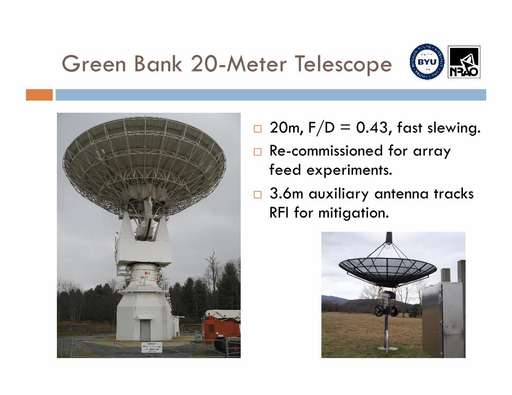
Green Bank 20-Meter Telescope
20m, F/D = 0.43, fast slewing. Re-commissioned for array
feed experiments. 3.6m auxiliary antenna tracks
RFI for mitigation.

BYU – NRAO 19 element array
Hexagonal grid of thickened 1.6 GHz dipoles. 0.6λ spacing, single polarization. 0.25λ offset from ground plane.

Analog RF front end
Downconversion to IF in front-end box behind array. 19 double conversion, room temperature analog receivers, Tsys ≈ 110K. Remotely tunable from 1200-2000MHz. IF bandwidth selectable at 0.5, 1.0, and 5.0 MHz. Connectorized modular system facilitates maintenance & channel isolation.
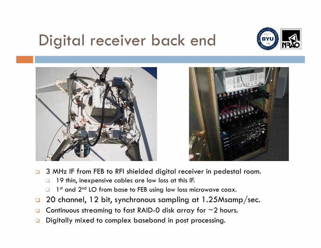
Digital receiver back end
3 MHz IF from FEB to RFI shielded digital receiver in pedestal room. 19 thin, inexpensive cables are low loss at this IF. 1st and 2nd LO from base to FEB using low loss microwave coax.
20 channel, 12 bit, synchronous sampling at 1.25Msamp/sec. Continuous streaming to fast RAID-0 disk array for ~2 hours. Digitally mixed to complex baseband in post processing.
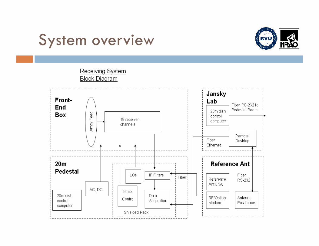
System overview
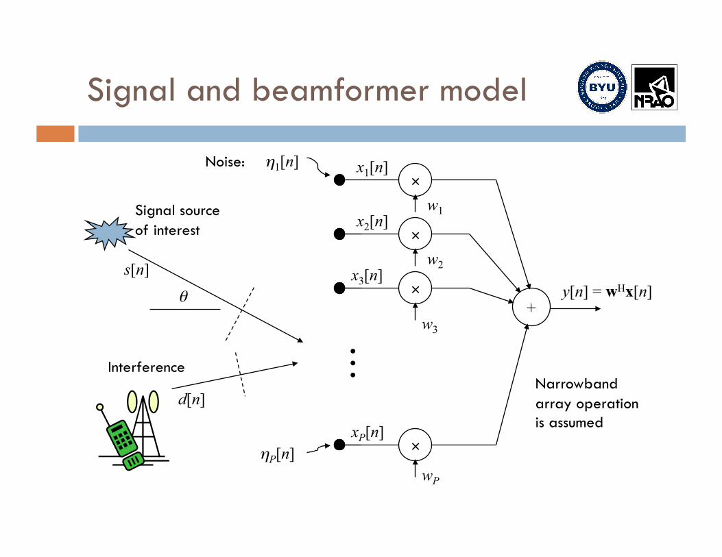
Signal and beamformer model
• • •
η1[n] x1[n]
x2[n]
+
×
w3
×
w1
×
w2
×
wP
y[n] = wHx[n]
xP[n]
s[n]
θ
Signal source of interest
x3[n]
ηP[n]
Noise:
d[n]
Interference Narrowband array operation is assumed
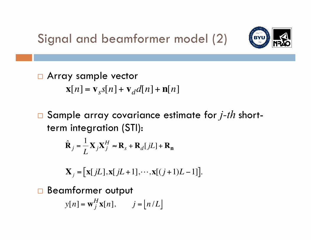
Signal and beamformer model (2)
Array sample vector
Sample array covariance estimate for j-th short-term integration (STI):
Beamformer output €
ˆ R j =1L
X jX jH ≈Rs + Rd[ jL] + Rn
€
X j = x[ jL],x[ jL +1],,x[( j +1)L −1][ ].
€
x[n] = vss[n]+ vdd[n]+ n[n]
€
y[n] = w jHx[n], j = n /L

Beamformer Definitions
Conjugate field match (CFM) from calibration data set. A.K.A. phase conjugate weighting, or spatial matched filter. Max SNR solution for i.i.d. noise.
LCMV Columns of C are distinct calibration constraint vectors. f is desired response in constraint directions, Single mainlobe constraint case (MVDR):
€
w j = ˆ v s, ˆ v s
€
w j = ˆ R j−1C[CH ˆ R j
−1C]−1f,
€
w jHC = f.
€
w j =ˆ R j−1 ˆ v s
ˆ v sH ˆ R j
−1 ˆ v s
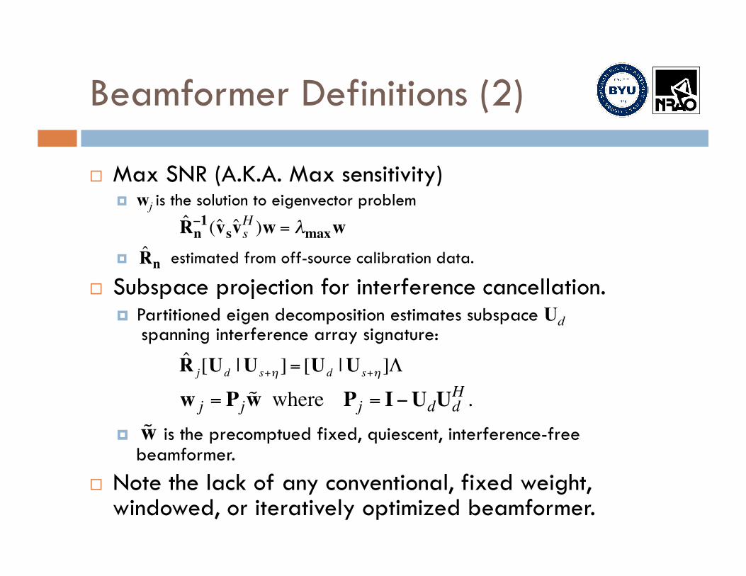
Beamformer Definitions (2)
Max SNR (A.K.A. Max sensitivity) wj is the solution to eigenvector problem
estimated from off-source calibration data. Subspace projection for interference cancellation.
Partitioned eigen decomposition estimates subspace Ud spanning interference array signature:
is the precomptued fixed, quiescent, interference-free beamformer.
Note the lack of any conventional, fixed weight, windowed, or iteratively optimized beamformer.
€
ˆ R n−1(ˆ v s ˆ v s
H )w = λmaxw
€
ˆ R n
€
ˆ R j[Ud | U s+η ] = [Ud | U s+η ]Λ
€
w j = Pj ˜ w where Pj = I−UdUdH .
€
˜ w
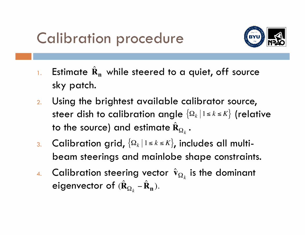
Calibration procedure
1. Estimate while steered to a quiet, off source sky patch.
2. Using the brightest available calibrator source, steer dish to calibration angle (relative to the source) and estimate .
3. Calibration grid, , includes all multi-beam steerings and mainlobe shape constraints.
4. Calibration steering vector is the dominant eigenvector of
€
ˆ R n
€
ˆ R Ωk
€
Ωk 1≤ k ≤ K{ }
€
Ωk 1≤ k ≤ K{ }
€
ˆ v Ωk
€
( ˆ R Ωk− ˆ R n ).
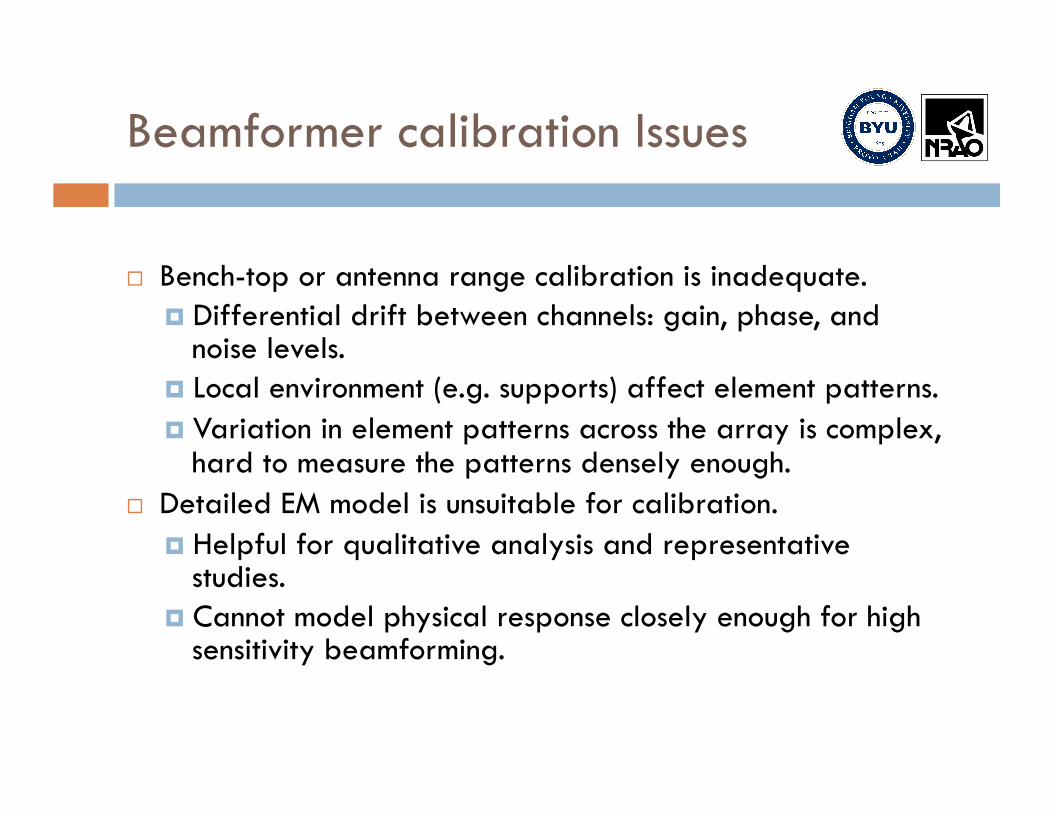
Beamformer calibration Issues
Bench-top or antenna range calibration is inadequate. Differential drift between channels: gain, phase, and
noise levels. Local environment (e.g. supports) affect element patterns. Variation in element patterns across the array is complex,
hard to measure the patterns densely enough. Detailed EM model is unsuitable for calibration.
Helpful for qualitative analysis and representative studies.
Cannot model physical response closely enough for high sensitivity beamforming.
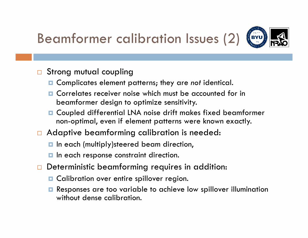
Beamformer calibration Issues (2)
Strong mutual coupling Complicates element patterns; they are not identical. Correlates receiver noise which must be accounted for in
beamformer design to optimize sensitivity. Coupled differential LNA noise drift makes fixed beamformer
non-optimal, even if element patterns were known exactly. Adaptive beamforming calibration is needed:
In each (multiply)steered beam direction, In each response constraint direction.
Deterministic beamforming requires in addition: Calibration over entire spillover region. Responses are too variable to achieve low spillover illumination
without dense calibration.
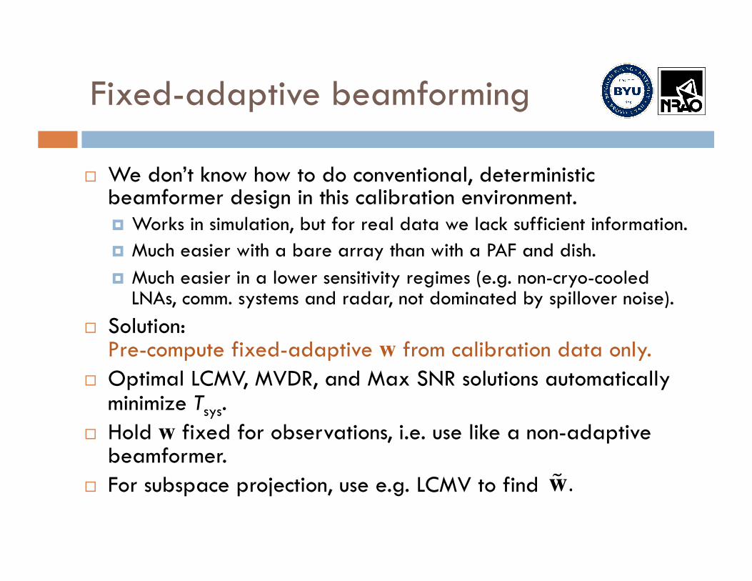
Fixed-adaptive beamforming
We don’t know how to do conventional, deterministic beamformer design in this calibration environment. Works in simulation, but for real data we lack sufficient information. Much easier with a bare array than with a PAF and dish. Much easier in a lower sensitivity regimes (e.g. non-cryo-cooled
LNAs, comm. systems and radar, not dominated by spillover noise). Solution:
Pre-compute fixed-adaptive w from calibration data only. Optimal LCMV, MVDR, and Max SNR solutions automatically
minimize Tsys. Hold w fixed for observations, i.e. use like a non-adaptive
beamformer. For subspace projection, use e.g. LCMV to find
€
˜ w .

Green Bank 20 Meter Telescope and EM simulations
Calibration and beamforming results

W49N, OH source detection
Conjugate field match (CFM) and LCMV beamformers were calculated from single pointing Cyg A calibration data.
10s observation, on-off source baseline subtraction. LCMV permits W49N detection. CFM spillover noise is too high.
!""#$% !""#$%# !""#$& !""#$&# !""#$' !""#$'# !""#$# !""#$## !""#$"
($#
!
!$#
%
%$#
)*!(!!' +,*-./012*3'45*6789*%(:*;7-9<*!4*2=2:2>8*?00?@
A02B/2>1@*7>*C,D
E.620*FG7>2?0<*?0H780?0@*-1?=2I
JAC*+>*K+L*EKM
JAC*+NN*K+L<*>.7-2*H?-2=7>2
GJCO*+>*K+L*EKM
GJCO*+NN*K+L<*>.7-2*H?-2=7>2
!""#$% !""#$%# !""#$& !""#$&# !""#$' !""#$'# !""#$# !""#$## !""#$"
(
($#
!
!$#
%
%$#
)*!(!!# +,*-./012*34,/-*.55*-./0126*7'89
:02;/2,1<*4,*=>[email protected]*BC4,2D06*D0E4F0D0<*-1DG2H
CI=J*E2DD35.0320
I:=*E2D35.0320
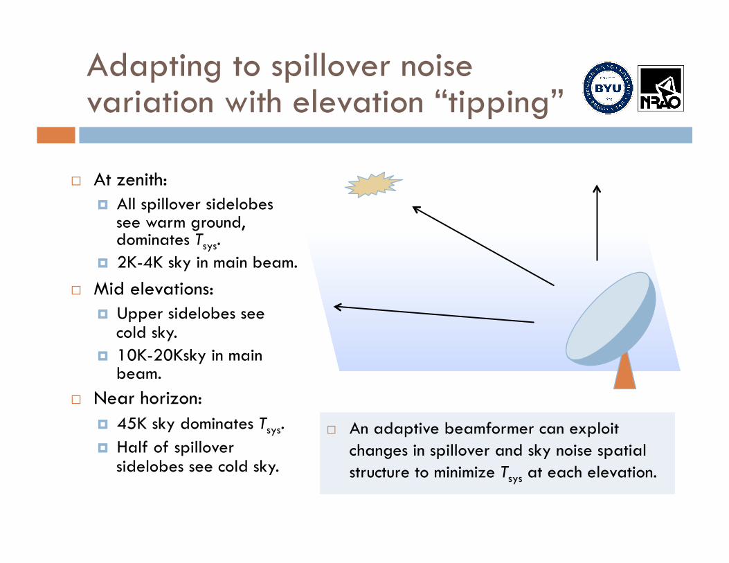
Adapting to spillover noise variation with elevation “tipping”
At zenith: All spillover sidelobes
see warm ground, dominates Tsys.
2K-4K sky in main beam. Mid elevations:
Upper sidelobes see cold sky.
10K-20Ksky in main beam.
Near horizon: 45K sky dominates Tsys. Half of spillover
sidelobes see cold sky.
An adaptive beamformer can exploit changes in spillover and sky noise spatial structure to minimize Tsys at each elevation.
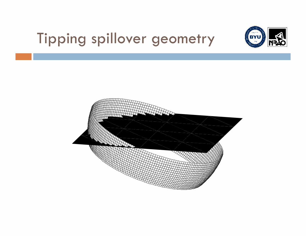
Tipping spillover geometry
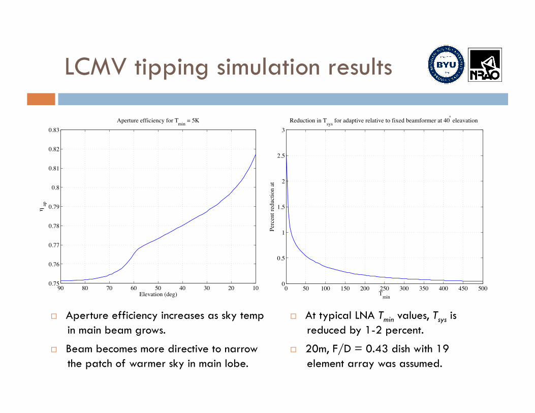
LCMV tipping simulation results
Aperture efficiency increases as sky temp in main beam grows.
Beam becomes more directive to narrow the patch of warmer sky in main lobe.
1020304050607080900.75
0.76
0.77
0.78
0.79
0.8
0.81
0.82
0.83
Elevation (deg)
! ap
Aperture efficiency for Tmin
= 5K
0 50 100 150 200 250 300 350 400 450 5000
0.5
1
1.5
2
2.5
3
Reduction in Tsys
for adaptive relative to fixed beamformer at 40° eleavation
Tmin
Per
cent
reduct
ion a
t
At typical LNA Tmin values, Tsys is reduced by 1-2 percent.
20m, F/D = 0.43 dish with 19 element array was assumed.

Tipping simulation results
Noise power (arbitrary scale) drops at lower elevations as LCMV adapts to changes in the noise spatial structure.
This simulation used Tmin = 120K to match the experimental system.
!"#"$"%"&"'"(")"*"'+'
'+'&
'+(
'+(&
'+)
'+)&
'+*
'+*&
(
(+"&
(+!,-!"
!&
./0123456-7809:
;54<0-=5>0?
@A<30B-654<0-=5>0?-2<-2-CD6E3456-5C-84<F-0/0123456-269/0
GHIJ-C4,08-23-K0643F
GHIJ-L82=3410
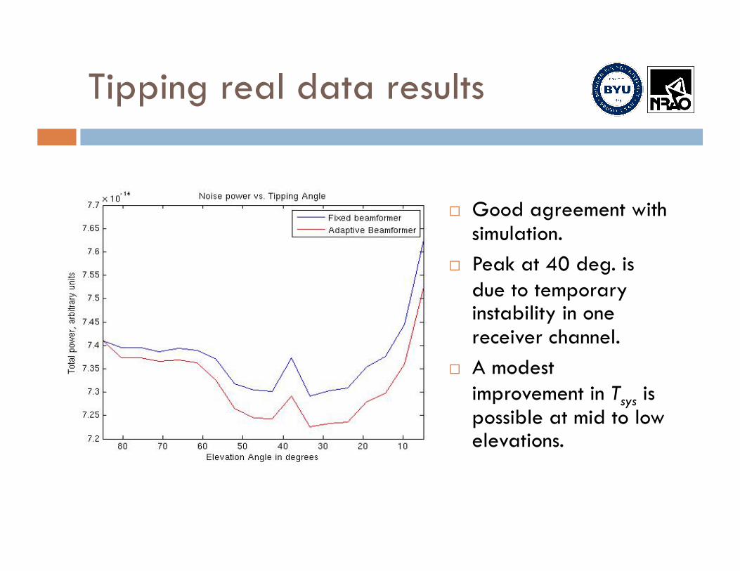
Tipping real data results
Good agreement with simulation.
Peak at 40 deg. is due to temporary instability in one receiver channel.
A modest improvement in Tsys is possible at mid to low elevations.

Experimental beamformer responses Green Bank 20m, 19 element data,
F/D = .43.
Stepped elevation slice across sky through Cyg A.
Beamformers: Center element only.
Conjugate filed match.
Max SNR (max sensitivity)
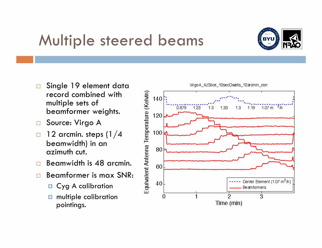
Multiple steered beams
Single 19 element data record combined with multiple sets of beamformer weights.
Source: Virgo A 12 arcmin. steps (1/4
beamwidth) in an azimuth cut.
Beamwidth is 48 arcmin. Beamformer is max SNR:
Cyg A calibration multiple calibration
pointings.

Sensitivity for off-axis beams
Model Details: Element patterns: Ansoft HFSS (FEM) Array mutual impedance matrix: HFSS Reflector: Physical optics (PO), no blockage or feed support scattering Receiver noise: Network model LNA noise parameters: Tmin = 100 K, Zopt = 45 + j5 Ω, Rn = 5 Ω
Boresight Beam (Model) Aperture efficiency: 79% Spillover efficiency: 97% Beam equivalent Trec: 127K Beam equivalent Tsys: 134K Sensitivity: 1.85 m2/K
Boresight Beam (Experiment) Sensitivity: 1.33 m2/K Aperture efficiency (@Tsys = 134K): 57%
Due to large LNA Tmin, the beamformer finds a solution with relatively high aperture efficiency (79%) and low spillover efficiency (97%).
Beam equivalent Tsys is higher than the LNA Tmin due to array mutual coupling.

Adaptive noise cancellation
Subspace projection adaptive canceling beamformer.
Strong moving CW RFI source in deep sidelobes.
Dish was stepped in elevation through source, Cyg A
0 0.5 1 1.5 2100
150
200
250CygA_slice_RFI1600_0_mov.bin
Time (min)
Eq
uiv
ale
nt
Ante
nn
a T
em
pera
ture
(K
elv
in)
Fixed Beamformer (RFI Corrupted)
Subspace Projection
Future work
Real-data beampattern and sensitivity measurements for w pre-computed from EM models. How close can we get?
Study performance bounds for deterministic beamformers. Lower Trec,Tsys experiments, ~35K, July 2008. 37 element array soon. Larger grids and longer integrations for calibration data. RFI mitigation
Null depth improvement. Beampattern control and adaptive bias removal.