Calculus: Intuitive Explanations

Radon Rosborough

https://intuitiveexplanations.com/math/calculus-intuitive-explanations/

Intuitive Explanations is a collection of clear, easy-to-understand, intuitive explanations of manyof the more complex concepts in calculus. In this document, an “intuitive” explanation is not onewithout any mathematical symbols. Rather, it is one in which each definition, concept, and part ofan equation can be understood in a way that is more than “a piece of mathematics”. For instance,some textbooks simply define mathematical terms, whereas Intuitive Explanations explains whatidea each term is meant to represent and why the definition has to be the way it is in order forthat idea to be captured. As another example, the proofs in Intuitive Explanations avoid steps withno clear motivation (like adding and subtracting the same quantity), so that they seem naturaland not magical. See the table of contents for information on what topics are covered. Beforeeach section, there is a note clarifying what prerequisite knowledge about calculus is required tounderstand the material presented. Section 1 contains a number of links to other resources useful forlearning calculus around the Web. I originally wrote Intuitive Explanations in high school, duringthe summer between AP Calculus BC and Calculus 3, and the topics covered here are, generallyspeaking, the topics that are covered poorly in the textbook we used (Calculus by Ron Larson andBruce Edwards, tenth edition).

Contents1 About Intuitive Explanations . . . . . . . . . . . . . . . . . . . . . . . . . . . . . . . . . 42 The Formal Definition of Limit . . . . . . . . . . . . . . . . . . . . . . . . . . . . . . . . 5

2.1 First Attempts . . . . . . . . . . . . . . . . . . . . . . . . . . . . . . . . . . . . . . 62.2 Arbitrary Closeness . . . . . . . . . . . . . . . . . . . . . . . . . . . . . . . . . . . . 72.3 Using Symbols . . . . . . . . . . . . . . . . . . . . . . . . . . . . . . . . . . . . . . 92.4 Examples . . . . . . . . . . . . . . . . . . . . . . . . . . . . . . . . . . . . . . . . . 9

2.4.1 Linear Function . . . . . . . . . . . . . . . . . . . . . . . . . . . . . . . . . . 92.4.2 Limit Rules . . . . . . . . . . . . . . . . . . . . . . . . . . . . . . . . . . . . 112.4.3 Quadratic Function . . . . . . . . . . . . . . . . . . . . . . . . . . . . . . . . 112.4.4 Disproving Limits . . . . . . . . . . . . . . . . . . . . . . . . . . . . . . . . . 132.4.5 Pathological Function . . . . . . . . . . . . . . . . . . . . . . . . . . . . . . . 15

2.5 Nuances . . . . . . . . . . . . . . . . . . . . . . . . . . . . . . . . . . . . . . . . . . 162.6 Extending the Definition . . . . . . . . . . . . . . . . . . . . . . . . . . . . . . . . . 16

2.6.1 Infinite Limits . . . . . . . . . . . . . . . . . . . . . . . . . . . . . . . . . . . 172.6.2 Limits of Sequences . . . . . . . . . . . . . . . . . . . . . . . . . . . . . . . . 172.6.3 Limits in Multiple Dimensions . . . . . . . . . . . . . . . . . . . . . . . . . . 172.6.4 Riemann Sums . . . . . . . . . . . . . . . . . . . . . . . . . . . . . . . . . . 18

3 Differentiation . . . . . . . . . . . . . . . . . . . . . . . . . . . . . . . . . . . . . . . . . . 183.1 The Product Rule . . . . . . . . . . . . . . . . . . . . . . . . . . . . . . . . . . . . . 183.2 The Quotient Rule . . . . . . . . . . . . . . . . . . . . . . . . . . . . . . . . . . . . 18

4 Integration . . . . . . . . . . . . . . . . . . . . . . . . . . . . . . . . . . . . . . . . . . . 194.1 The Formal Definition of the Integral . . . . . . . . . . . . . . . . . . . . . . . . . . 19

4.1.1 The Idea . . . . . . . . . . . . . . . . . . . . . . . . . . . . . . . . . . . . . . 194.1.2 Calculating Area . . . . . . . . . . . . . . . . . . . . . . . . . . . . . . . . . 204.1.3 Using Limits . . . . . . . . . . . . . . . . . . . . . . . . . . . . . . . . . . . . 224.1.4 Implications . . . . . . . . . . . . . . . . . . . . . . . . . . . . . . . . . . . . 24

4.2 The First Fundamental Theorem of Calculus . . . . . . . . . . . . . . . . . . . . . . 254.2.1 The Form of the Equation . . . . . . . . . . . . . . . . . . . . . . . . . . . . 254.2.2 The Main Idea . . . . . . . . . . . . . . . . . . . . . . . . . . . . . . . . . . 254.2.3 The Details . . . . . . . . . . . . . . . . . . . . . . . . . . . . . . . . . . . . 264.2.4 Alternate Proof . . . . . . . . . . . . . . . . . . . . . . . . . . . . . . . . . . 274.2.5 Conclusion . . . . . . . . . . . . . . . . . . . . . . . . . . . . . . . . . . . . . 28

4.3 The Second Fundamental Theorem of Calculus . . . . . . . . . . . . . . . . . . . . . 295 Sequences and Series . . . . . . . . . . . . . . . . . . . . . . . . . . . . . . . . . . . . . . 29

5.1 Bounded Monotonic Sequences . . . . . . . . . . . . . . . . . . . . . . . . . . . . . 305.2 The Integral Test and Remainder Formula . . . . . . . . . . . . . . . . . . . . . . . 315.3 The Limit Comparison Test . . . . . . . . . . . . . . . . . . . . . . . . . . . . . . . 345.4 The Alternating Series Test and Remainder Formula . . . . . . . . . . . . . . . . . 355.5 The Ratio and Root Tests . . . . . . . . . . . . . . . . . . . . . . . . . . . . . . . . 36

6 Vector Analysis . . . . . . . . . . . . . . . . . . . . . . . . . . . . . . . . . . . . . . . . . 406.1 The Gradient . . . . . . . . . . . . . . . . . . . . . . . . . . . . . . . . . . . . . . . 40

6.1.1 Intuition . . . . . . . . . . . . . . . . . . . . . . . . . . . . . . . . . . . . . . 406.1.2 Definition . . . . . . . . . . . . . . . . . . . . . . . . . . . . . . . . . . . . . 406.1.3 Definition with Partial Derivatives . . . . . . . . . . . . . . . . . . . . . . . 44

6.2 The Gradient Theorem . . . . . . . . . . . . . . . . . . . . . . . . . . . . . . . . . . 44

2

6.2.1 The Equation . . . . . . . . . . . . . . . . . . . . . . . . . . . . . . . . . . . 446.2.2 The Proof . . . . . . . . . . . . . . . . . . . . . . . . . . . . . . . . . . . . . 45

6.3 The Divergence . . . . . . . . . . . . . . . . . . . . . . . . . . . . . . . . . . . . . . 466.3.1 Intuition . . . . . . . . . . . . . . . . . . . . . . . . . . . . . . . . . . . . . . 466.3.2 Definition . . . . . . . . . . . . . . . . . . . . . . . . . . . . . . . . . . . . . 486.3.3 Definition with Partial Derivatives . . . . . . . . . . . . . . . . . . . . . . . 49

6.4 The Divergence Theorem . . . . . . . . . . . . . . . . . . . . . . . . . . . . . . . . . 516.5 The Curl . . . . . . . . . . . . . . . . . . . . . . . . . . . . . . . . . . . . . . . . . . 52

6.5.1 Intuition . . . . . . . . . . . . . . . . . . . . . . . . . . . . . . . . . . . . . . 526.5.2 Definition . . . . . . . . . . . . . . . . . . . . . . . . . . . . . . . . . . . . . 536.5.3 Definition with Partial Derivatives . . . . . . . . . . . . . . . . . . . . . . . 54

6.6 Green’s Theorem . . . . . . . . . . . . . . . . . . . . . . . . . . . . . . . . . . . . . 566.7 Stokes’ Theorem . . . . . . . . . . . . . . . . . . . . . . . . . . . . . . . . . . . . . 58

6.7.1 The Divergence of the Curl . . . . . . . . . . . . . . . . . . . . . . . . . . . 586.8 Conservative Vector Fields . . . . . . . . . . . . . . . . . . . . . . . . . . . . . . . . 59

6.8.1 Path Independence . . . . . . . . . . . . . . . . . . . . . . . . . . . . . . . . 606.8.2 Potential Functions . . . . . . . . . . . . . . . . . . . . . . . . . . . . . . . . 616.8.3 The Conservation of Energy . . . . . . . . . . . . . . . . . . . . . . . . . . . 636.8.4 No Circulation . . . . . . . . . . . . . . . . . . . . . . . . . . . . . . . . . . 646.8.5 No Curl . . . . . . . . . . . . . . . . . . . . . . . . . . . . . . . . . . . . . . 65

6.8.5.1 The Property . . . . . . . . . . . . . . . . . . . . . . . . . . . . . . 656.8.5.2 The Caveat . . . . . . . . . . . . . . . . . . . . . . . . . . . . . . . 656.8.5.3 The Topology . . . . . . . . . . . . . . . . . . . . . . . . . . . . . . 67

6.8.6 Summary . . . . . . . . . . . . . . . . . . . . . . . . . . . . . . . . . . . . . 67

3

1 About Intuitive ExplanationsSince I originally wrote Intuitive Explanations while reading my high school Calculus textbook,I happen to have a handy table correlating sections from that textbook to sections in IntuitiveExplanations:

Calculus by Larsonand Edwards

Topic Intuitive Explanations

Chapter 1.3 The formal definition of limit Section 2Chapter 2.3 The product rule Section 3.1

The quotient rule Section 3.2Chapter 4.2, 4.3 The formal definition of the integral Section 4.1Chapter 4.4 The first fundamental theorem of

calculusSection 4.2

The second fundamental theorem ofcalculus

Section 4.3

Chapter 9.1 Bounded monotonic sequences Section 5.1Chapter 9.3 The integral test and remainder

formulaSection 5.2

Chapter 9.4 The limit comparison test Section 5.3Chapter 9.5 The alternating series test and

remainder formulaSection 5.4

Chapter 9.6 The ratio and root tests Section 5.5Chapter 13.6 The gradient Section 6.1Chapter 15.1, 15.3 Conservative vector fields Section 6.8Chapter 15.1 The curl Section 6.5

The divergence Section 6.3Chapter 15.2 The gradient theorem Section 6.2Chapter 15.4 Green’s theorem Section 6.6Chapter 15.7 The divergence theorem Section 6.4Chapter 15.8 Stokes’ theorem Section 6.7

Section numbers are hyperlinked: you can click on a number to jump to that section in thisdocument.

Additionally, following is a list of some places on the Web you can find more information andexplanations of things in Calculus; the text typeset in bold is hyperlinked. The list is roughlyordered from most to least useful, in my opinion:

The Feynman Technique has nothing per se to do with Calculus, but it can be used to greateffect to help learn Calculus (or anything else).

Math Insight is a website that covers many of the concepts in the third semester of Calculusfrom an intuitive standpoint. It includes many very helpful explanations and interactivevisualizations.

BetterExplained is a website with an even greater emphasis on intuition-first learning than thisdocument. It covers topics in everything from Arithmetic to Linear Algebra.

4

Paul’s Online Math Notes can essentially be used as a very easy-to-follow textbook for the firstthree semesters of Calculus as well as Differential Equations.

This fully geometric proof of the derivatives of sin and cos is nothing short of beautiful.

These notes about Lagrange multipliers are excellent and provide a concrete, graphical, in-tuitive explanation of Lagrange multipliers that I have not seen anything else come closeto.

This Math StackExchange thread contains several very appealing explanations of why the de-terminant has the properties it does.

This Math StackExchange thread contains a concrete, intuitive example that instantly demys-tified the Extended Mean Value Theorem (used in the proof of l’Hôpital’s rule) for me.

This article on Riemann’s Rearrangment Theorem not only provides an excellent proof ofsaid astonishing theorem but also grants much deeper insight into the fundamental naturesof absolutely and conditionally convergent series.

The Interactive Gallery of Quadric Surfaces has a variety of useful visualizations, insights,and tips relating to quadric surfaces.

Math StackExchange is always a useful resource, although whether any given answer will beuseful to you is more or less up to the flip of a coin.

Wolfram|Alpha is a “computational knowledge engine” with breathtaking breadth and depth. Itcan solve the vast majority of elementary, computational math problems, and will sometimesprovide step-by-step solutions if you buy a subscription for a few dollars.

These notes about curvature contain a number of useful facts and proofs that I was unable tofind elsewhere.

These notes about improper double integrals contain some formal definitions and theoremsthat I was unable to find elsewhere.

These notes about the second partials test contains some details of its generalization to func-tions of n variables that I was unable to find elsewhere.

2 The Formal Definition of LimitPrerequisite Knowledge. Understand generally what a limit is, and be able to evaluate limitsgraphically and numerically.

What, exactly, does it mean for a function to “have a limit” at a certain point? You haveprobably learned that the limit of a function at a point is related to the values of the function nearthat point, but that these two things are not quite the same. For instance, you are surely awarethat the first two functions depicted in figure 2.1 both have the limit L at x = c, while the thirdfunction does not have any limit at x = c.

But what about the function

f(x) =

{x if x is rational0 if x is irrational ?

5

L

c

limx→c f(x) = L = f(c)

L

c

limx→c f(x) = L ̸= f(c)

c

limx→c f(x) does not exist

Figure 2.1: Functions with different behaviors at x = c and their limits at that point.

It would be very difficult to graph this function. Does it have a limit anywhere? If so, where?It is not easy to tell without a precise definition of limit. In this section, we will develop justsuch a definition. We will start with a simple, straightforward definition and gradually improve itsweaknesses until we reach a more complex but completely watertight definition that can be appliedto any function whatsoever.

You might wonder what the point of all this is. And indeed, it is certainly possible to understandalmost everything in calculus quite well without knowledge of the formal definition of limit. Buton the other hand, literally everything in calculus is based on the formal definition of limit – andso you will gain a much deeper understanding of how calculus works by taking the time to studylimits in detail.

2.1 First AttemptsThink about how you determine limits from a graph. The main idea is to figure out what thevalue of the function is “heading towards” as x approaches c without actually using the value of thefunction at x = c.

For example, take the second graph pictured in figure 2.1. We know that the limit ought to beL at x = c, but why? One answer is, “f(x) becomes very close to L near (but not at) x = c.” Thisleads to a definition of what it means for the statement

limx→c

f(x) = L

to be true.

Definition. limx→c f(x) = L if f(x) becomes very close to L as x approaches (but does notreach) c.

Unfortunately, this definition is no good in a proof. What does “very close” mean? Reasonablepeople could disagree over whether 1.001 is “very close” to 1. Let’s try defining “very close” – forinstance, “differing by less than 0.01” might seem reasonable.

Definition. limx→c f(x) = L if f(x) comes within 0.01 of L as x approaches (but does notreach) c.

Here, as well as later, “x is within 0.01 of y” means that the value of x and the value of y differby less than 0.01: that the distance between x and y on a number line is less than 0.01. In symbols,|x− y| < 0.01.

6

L

c

y = f(x) = x(1, 1)

(1, 1.001)

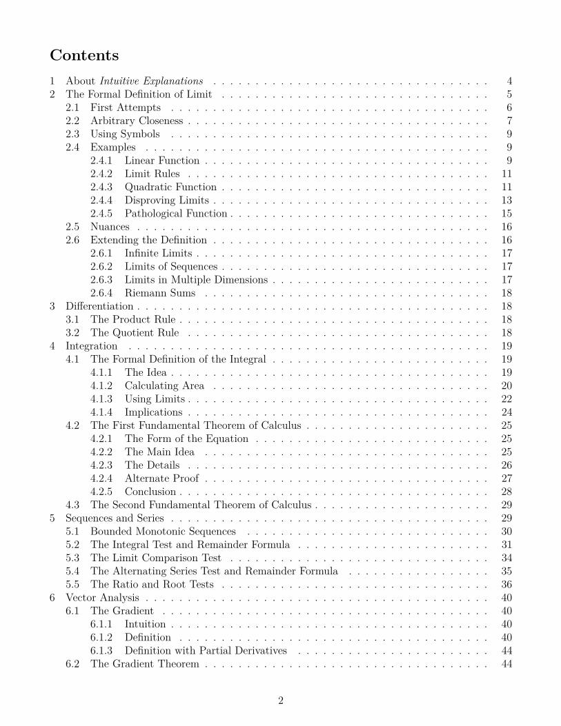
Figure 2.2: According to our second definition, limx→1 x = 1.001. (Here, c = 1, L = 1.001, andf(x) = x.) This is because near x = 1, the difference between f(x) and L = 1.001 is approximately0.001. And according to our definition, all f(x) has to do for its limit to exist is come within 0.01 ofL = 1.001 near x = c = 1. In fact, you can use this same reasoning to show that limx→1 x is equalto an infinite number of different values, which is clearly ridiculous.

This definition probably seems a little off to you: after all, we do not want a function f(x) thatcomes within 0.01 of L, but just barely misses. We want a function that actually “hits” the point(c, L), like the second function shown in figure 2.1. A near miss that would satisfy this definition isshown in figure 2.2.

2.2 Arbitrary ClosenessYou can probably see that no matter what numerical requirement we put on how close f(x) mustbe to L, it will still be possible for f(x) to satisfy that requirement, but still “just miss” (c, L). Sohow can we separate functions like the first two in figure 2.1 from the one pictured in figure 2.2?

The key principle is that functions that “pass through” their limiting point (c, L) will be ableto satisfy any requirement on how close f(x) must get to L. For instance, if you zoomed in on thesecond graph in figure 2.1, you would see that f(x) comes within 0.01 of L. But if you zoomed infarther, you would also see that it comes within 0.0001 of L; if you zoomed in unimaginably far,you would see f(x) come within even 10−1000 of L. This type of zoom is depicted in figure 2.3.

Keeping in mind the property of being able to satisfy any requirement on how close f(x) mustget to L, we can write a new definition.

Definition. limx→c f(x) = L if f(x) can satisfy any requirement on how close it must be to L(once x gets close enough to c).

Let’s rephrase a few parts of this definition to make everything more explicit:

Definition. limx→c f(x) = L if: For any requirement that f(x) be within a certain distance ofL, that requirement is satisfied when x is sufficiently close to c.

Definition. limx→c f(x) = L if: For any requirement that f(x) be within a certain distanceof L, there is a second requirement that x be within a certain distance of c such that the firstrequirement is satisfied whenever the second requirement is satisfied.

7

c

L

L− ϵ

L+ ϵ

Figure 2.3: A small portion of the second graph in figure 2.1, magnified so much that the graphappears as a straight line. The symbol ϵ represents a very small number, such as 10−1000. You cansee from the graph that when x is close enough to c, f(x) will come within ϵ of L (all of the valuesbetween L− ϵ and L+ ϵ are within ϵ of L). Notice that when you zoom in even more, the graphwill look exactly the same, but ϵ will become an even smaller number. This shows that no matterhow small of a number ϵ you can think of, f(x) will eventually get within that distance of L (oncex is close enough to c).

L+ ϵ

L− ϵ

c+ δc− δ 1

1

L

c

Figure 2.4: A visual representation of the fact that limx→0.7 x2 = 0.49. In this figure (to scale),

f(x) = x2, c = 0.7, δ = 0.075, L = 0.49, and ϵ = 0.15, but many other values would produce asituation similar to the one shown.

Make sure you understand this last definition, because it is essentially the same as the finaldefinition – just in words instead of symbols. An example, for the function f(x) = x2, is picturedin figure 2.4.

The first requirement in our definition is that f(x) be within ϵ = 0.15 of L = 0.49, which isequivalent to f(x) being within the blue band. The second requirement is that x be within δ = 0.075of c = 0.7, which is equivalent to x being within the red band. You can see in figure 2.4 that everypoint on y = f(x) that is contained in the red band is also contained in the blue band. (This is aconsequence of the olive-colored projection of the red band being entirely contained within the blue

8

band.) Therefore, the first requirement is satisfied whenever the second requirement is satisfied. Inorder for the limit limx→0.7 x

2 = 0.49 to exist according to our definition, it must always be possibleto draw a red band whose projection lies entirely within the blue band, no matter how thin the blueband is made.

2.3 Using SymbolsIf you understand our last definition, it is a relatively simple matter to translate its words intosymbols. (Of course, what you should remember are the words, not the symbols – but on the otherhand, it is easier to do proofs with symbols than with words.)

Firstly, a requirement that x be within a certain distance of y can be described with a singlenumber: the distance (call it D). This requirement is satisfied when |x − y| < D. So, the firstrequirement in the definition – that f(x) be within a certain distance of L – can be described with asingle number, which we will call ϵ. This requirement is satisfied when |f(x)− L| < ϵ. Analogously,the second requirement – that x be within a certain distance of c – can be described with anothernumber, which we will call δ. This requirement is satisfied when |x− c| < δ.

We can now make some substitutions in our last definition:

limx→c f(x) = L if: limx→c f(x) = L if:For any requirement that f(x) be within acertain distance of L,

For any positive number ϵ,

there is a second requirement that x bewithin a certain distance of c such that

there is a positive number δ such that

the first requirement is satisfied wheneverthe second requirement is satisfied.

|f(x)− L| < ϵ whenever |x− c| < δ.

This gives us a concise and very precise final1 definition:

Definition. limx→c f(x) = L if for every positive number ϵ there is at least one positive numberδ such that |f(x)− L| < ϵ whenever |x− c| < δ.

By the way, if you’re wondering where the letters ϵ and δ came from, ϵ is the lowercase Greek let-ter “epsilon” and originally stood for “error”, while δ is the lowercase Greek letter “delta” (uppercase∆), which stands for change.

2.4 Examples2.4.1 Linear Function

limx→2

3x = 6

If we plug in f(x) = 3x, c = 2, and L = 6 to our definition, then we get:

Definition. limx→2 3x = 6 if for every positive number ϵ there is at least one positive numberδ such that |3x− 6| < ϵ whenever |x− 2| < δ.

Figure 2.5 illustrates the situation for this limit.1Well, not quite. See section 2.5 for the real, unabridged final version.

9

c− δ c+ δ

L− ϵ

L+ ϵ y = f(x) = 3x

c

L

Figure 2.5: Values of ϵ and δ that satisfy our definition of limit.

Our definition asserts that for every number ϵ, there is a number δ that meets a certain specificcondition (if the limit exists, which limx→2 3x = 6 does). Pictured in figure 2.5 is an arbitraryvalue of ϵ and a value of δ that meets the condition of the definition, which is that |3x− 6| < ϵwhenever |x− 2| < δ. You can see in the figure that if |x− 2| < δ (meaning that x is within the redband), then |3x− 6| < ϵ (meaning that f(x) = 3x is within the blue band). Just as before, this isa consequence of the projection of the red band being entirely within the blue band. You can alsosee that if the red band were made narrower, then the same property would hold true: Therefore,there are many values of δ that are valid for any given ϵ, not just one. Finally, note that no matterhow small the blue band were to be made, the red band could be made small enough so that itsprojection laid once more entirely within the blue band. This shows that our definition holds true,and so that limx→2 3x = 6 exists.

Now that you understand what is going on in the formal definition of limit, we are ready to useit to formally prove an actual limit – in this case, limx→2 3x = 6. The math is very easy – the hardpart is keeping track of when each statement and inequality is true.

According to our definition, we will have to prove a certain statement “for every positive numberϵ”. Let’s start by proving that statement (“there is at least one positive number δ such that|3x− 6| < ϵ whenever |x− 2| < δ”) for a single ϵ. If we let ϵ = 1/10, then we will have to provethat “there is at least one positive number δ such that |3x− 6| < 1/10 whenever |x− 2| < δ”.

The easiest way to prove that there is a number with a certain property (say, that it can bedivided evenly by 6 positive integers) is to come up with such a number (12) and then show thatthe number has the property it is supposed to (1, 2, 3, 4, 6, 12). We will do exactly the same thingin order to prove that there is a number δ with the property in our definition.

We can start by noting that |3x− 6| < 1/10 is equivalent to |x− 2| < 1/30 (by dividing bothsides by 3). Since this expression is quite similiar to |x− 2| < δ, we might try letting δ = 1/30.In that case, whenever |x− 2| < δ, it is also true that |x− 2| < 1/30, and so (as we said earlier)

10

|3x− 6| < 1/10, which is what we wanted to prove. Therefore, the statement “there is at least onepositive number δ such that |3x− 6| < ϵ whenever |x− 2| < δ” is true when ϵ = 1/10.

What about when ϵ is some other value? If you understood the above reasoning, extending itto any ϵ is quite easy: just replace 1/10 with ϵ, and replace 1/30 with ϵ/3. Since all we need to dois show that there is an appropriate value of δ for each possible value of ϵ, it is perfectly reasonableto need to know what ϵ is in order to figure out what δ ought to be. (On the other hand, you can’tuse x in your expression for δ. If you could, you could just say “δ = twice the distance between xand c”, and x would always be within δ of c no matter what limit you were trying to compute!)

That’s it! A typical textbook proof that limx→2 3x = 6 might go as follows, albeit probablywithout colors:

Suppose we are given ϵ > 0. Let δ = ϵ/3. If |x− 2| < δ, then |x− 2| < ϵ/3 and so |3x− 6| < ϵ.Therefore the limit exists.

Even if this proof is a little on the terse side, now that you know how to do the proof yourselfyou ought to be able to understand it.

As an exercise, prove that limx→−3(−5x) = 15. If you run into trouble, refer back to the proofthat limx→2 3x = 6.

2.4.2 Limit Rules

limx→c

kx = kc

There is really nothing new about this limit, since the last limit is just a special case of it, withc = 2 and k = 3. However, it is important to be able to prove limits that have variables in them –you just have to be able to keep track of which variables are changing, and when they do. Accordingto our definition:

Definition. limx→c kx = kc if for every positive number ϵ there is at least one positive numberδ such that |kx− kc| < ϵ whenever |x− c| < δ.

Here is a short proof, based on our previous one:

Suppose we are given ϵ > 0. Let δ = ϵ/|k|. If |x− c| < δ, then |x− c| < ϵ/|k| and so|kx− kc| < ϵ. Therefore the limit exists.

We use |k| instead of just k because k might be negative.Really, the best way to thoroughly understand the formal definition of limit (once you have

studied its basic principles) is to apply it yourself. Try to write proofs for the following limits:

• limx→c k = k

• limx→c(x+ 1) = c+ 1

• limx→c(kx− x) = kc− c

The best way to start is to rewrite the formal definition, plugging in the values for f(x) and L.

2.4.3 Quadratic Function

11

"This section has material much more difficult than that of the surrounding sections. You may

safely skip this section and proceed to the next if you are not particularly interested inquadratic functions.

limx→c

x2 = c2

Finding the limit of a quadratic function is surprisingly difficult, but it is a very good exercisein proof-writing. We will assume that c is positive because it makes the proof less tedious. Thedefinition says:

Definition. limx→c x2 = c2 if for every positive number ϵ there is at least one positive number

δ such that |x2 − c2| < ϵ whenever |x− c| < δ.

The first thing to do is to try to get the ϵ expression to look more similar to the δ expression.Recalling the properties that a2−b2 = (a+b)(a−b) and that |ab| = |a||b|, we see that |x2 − c2| < ϵ isequivalent to |x+ c||x− c| < ϵ. The only difference now is the extra |x+ c| term in the ϵ expression.Your first thought might be to let δ = ϵ/|x+ c|, but as we discussed earlier we cannot use x in ourexpression for δ. So what can we do?

In many of the more complex ϵ-δ proofs (such as this one), some of the steps you take will notbe symmetric. For instance, a symmetric step is from 2x < 4 to x < 2, while an asymmetric stepis from x < 2 to x < 3. Both are perfectly valid, but you can only reverse symmetric steps (x < 2implies 2x < 4, but x < 3 does not imply x < 2). This idea will come into play shortly.

First, however, let’s examine what possible magnitudes |x+ c| can have. Since we are trying toprove that |x− c| < δ implies |x+ c||x− c| < ϵ, we can assume that |x− c| < δ is true. This meansthat x is between c− δ and c+ δ. Therefore, x+ c must be between 2c− δ and 2c+ δ. Since c andδ are positive, −2c− δ is clearly less than 2c− δ. Thus, x+ c must also be between −2c− δ and2c+ δ, which means |x+ c| cannot be greater than 2c+ δ if |x− c| < δ.

So what was the point of all that? Well, remember how we cannot simply let δ = ϵ/|x+ c|because x cannot be present in our expression for δ? The solution is to use the inequality we foundabove to transform the expression |x+ c| into 2c+ δ, which does not have an x in it. To do so, wecan use the simple principle that if a ≤ b and bx < c, then ax < c. We know that |x+ c| < 2c+ δ,so if (2c+ δ)|x− c| < ϵ, then |x+ c||x− c| < ϵ.

However, we can’t exactly let δ = ϵ/(2c+ δ), as we would be led in endless circles if we ever triedto evaluate that expression. To resolve the problem, we can use another inequality. The key idea isto decide now that we will not let δ ever be more than c. We do not know what our expression forδ will be yet, but we’ll make sure to write it so that δ ≤ c. This means that we have the inequality2c+ δ ≤ 3c. Now, all we have to do is use the same principle as we used with |x+ c| < 2c+ δ, andwe can find that if 3c|x− c| < ϵ, then (2c+ δ)|x− c| < ϵ.

So what we have found is that if 3c|x− c| < ϵ, then |x+ c||x− c| < ϵ. This is almost what wewant! It is now quite natural to let δ = ϵ/3c, which would be correct if it were not for the fact thatwe also said earlier that we would make δ ≤ c. It’s relatively simple to satisfy this requirement,though – we can just let δ be whichever of ϵ/3c or c is smaller. This way, we know that δ cannotbe greater than c.

We have finally obtained a formula for δ! If you’d like to write it out symbolically, δ =min(ϵ/3c, c) would do nicely. We can now write out the actual proof that limx→c x

2 = c2 wherec > 0:

12

Suppose we are given ϵ > 0. Let δ be whichever of ϵ/3c or c is smaller. Now suppose that|x− c| < δ. Since δ ≤ ϵ/3c, we know that |x− c| < ϵ/3c, and so 3c|x− c| < ϵ. We alsohave that δ ≤ c, which means that 2c+ δ < 3c and so (2c+ δ)|x− c| < ϵ. Additionally, by ourreasoning earlier, |x− c| < δ implies that |x+ c| < 2c+ δ. Consequently |x+ c||x− c| < ϵ and|x2 − c2| < ϵ. Therefore the limit exists.

Figure 2.6 illustrates that the values of δ given by our formula δ = min(ϵ/3c, c) really do work.

1

1

L

c

c = 0.7 L = 0.49δ = 1/14 ϵ = 0.15

5

20

L

c

c = 3 L = 9δ = 1/18 ϵ = 0.5

L

cc = 0.2 L = 0.04δ = 1/60 ϵ = 0.01

Figure 2.6: Various values of ϵ and the corresponding values of δ for the function f(x) = x2.

Note, by the way, that c must be included along with ϵ/3c in the formula for δ because it keepsproblems from cropping up for large values of ϵ. For instance, if c = 1, L = 1, and ϵ = 30, then thesimple formula δ = ϵ/3c would give us δ = 10. Unfortunately, x = 10 is within δ = 10 of c = 1, butf(x) = 100 is definitely not within ϵ = 30 of L = 1. On the other hand, the more complex formulaδ = min(ϵ/3c, c) gives us the much smaller δ = 1. All is well.

It might seem silly that we have to worry about large values of ϵ (which we normally think ofas a small number), but such is the price of rigor.

2.4.4 Disproving Limits

limx→0

1

xdoes not exist

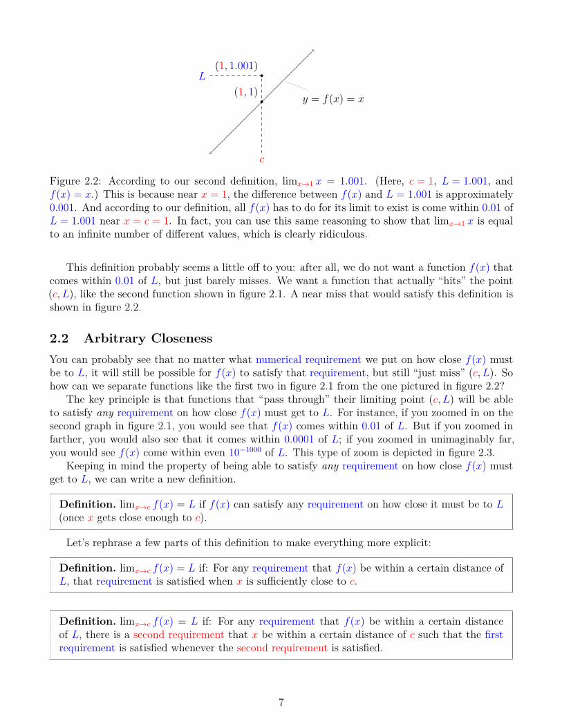
You are doubtless already familiar with limits that do not exist, such as the one above (picturedin figure 2.7). It is also possible to use the formal definition of limit to prove this fact.

Of course, first we need to know what it means for a limit not to exist. Here is the definition:

Definition. limx→c f(x) does not exist if the statement limx→c f(x) = L is not true for anynumber L.

In other words, if the limit does not have any value, then it does not exist. We can expand thisas:

13

f(x) = 1/x

Figure 2.7: A function that has no limit at x = 0.

Definition. limx→c f(x) does not exist if for every number L the following is false: for everypositive number ϵ there is at least one positive number δ such that |f(x)− L| < ϵ whenever|x− c| < δ.

We can rephrase the above definition using De Morgan’s laws. You may think you have notheard of these, but in fact you use them all the time. For instance, one of De Morgan’s laws statesthat if it is false that “all ravens are black”, then it is true that “at least one raven is non-black”.Conversely, if it is false that “at least one raven is yellow”, then it is true that “all ravens arenon-yellow”.

You should be able to convince yourself that the above definition and the below definition areequivalent.

Definition. limx→c f(x) does not exist if for every number L there is at least one positivenumber ϵ for which there is no positive number δ such that |f(x)− L| < ϵ whenever |x− c| < δ.

Intuitively, why does limx→0 1/x not exist? As x gets closer to c = 0 from the right, f(x) = 1/xwill get larger and larger. In fact, no matter what number L you pick, f(x) will grow larger thanL, then larger than 2L, then larger than 1000L as x continues to approach c = 0. Therefore, f(x)does not get closer and closer to any single number as x approaches c, and consequently the limitdoes not exist.

The above definition, written for our particular limit, is as follows:

Definition. limx→0 1/x does not exist if for every number L there is at least one positive numberϵ for which there is no positive number δ such that |1/x− L| < ϵ whenever |x| < δ.

Here is a proof:

Suppose we are given a number L. Let ϵ = L. We would like to show that there is no positivenumber δ such that |1/x− L| < ϵ whenever |x| < δ, so suppose we are given an arbitrary δ > 0.Consider x = min(δ/2, 1/(2|L|)). We know that 0 < x ≤ δ/2, so it is certainly true that |x| < δ.However, we also have that x ≤ 1/(2|L|), so 1/x ≥ 2|L|. Consequently, 1/x− L ≥ |L| (becausesubtracting L cannot reduce the right-hand side by more than |L|). From this we can concludethat |1/x− L| ≥ L. Since there is at least one value of x for which |x| < δ but not |1/x− L| < ϵ

14

(remember that ϵ = L) – and there is one such value for any possible value of δ – we have provedthat there is no positive number δ such that |1/x− L| < ϵ whenever |x| < δ. Since we showedthat this is true for at least one value of ϵ no matter what the value of L is, we have proved thestatement in the definition.

The validity of the values of ϵ and x produced in this proof is illustrated in figure 2.8.

L

x

δ = 0.75, x = δ/2 = 0.375

L

x

δ = 1.25, x = 1/(2|L|) = 0.5

(note that because we use < instead of ≤ in|f(x)− L| < ϵ, being on the edge of a band doesnot count)

Figure 2.8: Here, an example value of L = 1 was chosen. Our proof gives ϵ = L = 1, which generatesthe blue bands centered around L in the graphs. Next an example value of δ was chosen, which gener-ates the red bands centered around c = 0 in the graphs. Our proof then gives x = min(δ/2, 1/(2|L|)),which is inside the red band without f(x) being inside the blue band – in both cases, just as weproved.

2.4.5 Pathological Function

Recall the functionf(x) =

{x if x is rational0 if x is irrational

from page 5. It turns out that limx→c f(x) is 0 for c = 0 but the limit does not exist for c ̸= 0.Why?

Definition. limx→0 f(x) = 0 if for every positive number ϵ there is at least one positive numberδ such that |f(x)| < ϵ whenever |x| < δ.

To prove this, simply let δ = ϵ. If |x| < δ, then since |f(x)| ≤ |x|, we can use transitivity toconclude that |f(x)| < ϵ.

The fact that limx→c f(x) does not exist for c ̸= 0 is a consequence of the fact that every possibleinterval of real numbers contains both rational numbers and irrational numbers. This means thatany interval (of width δ, say) containing x = c will also contain some rational numbers greater thanc and some irrational numbers greater than c. Therefore, if we look at the definition of f(x), we

15

notice that in any interval containing x = c, f(x) will be 0 at some points and greater than c atsome points. All we have to do to prove that the limit does not exist, then, is to pick an ϵ smallerthan c/2, because no interval of height less than c will be able to include both 0 and values greaterthan c.

2.5 NuancesOur formal definition is currently as follows:

Definition. limx→c f(x) = L if for every positive number ϵ there is at least one positive numberδ such that |f(x)− L| < ϵ whenever |x− c| < δ.

Notice that it says |f(x)− L| < ϵ should be true for any x where |x− c| < δ. But what aboutx = c? Our definition of a limit should not depend on f(c), because of functions like the secondone shown in figure 2.1. (In fact, according to our current definition, only continuous functions canhave limits!) So actually, we only want to consider values of x for which 0 < |x− c| < δ. The onlyreason we did not write this earlier was for conciseness. Therefore, a more correct definition is:

Definition. limx→c f(x) = L if for every positive number ϵ there is at least one positive numberδ such that |f(x)− L| < ϵ whenever 0 < |x− c| < δ.

The one final modification to our definition of limit involves the fact that

limx→0

√x does not exist

according to our current definition.First, let’s discuss why this is the case. For this limit c = 0, so no matter what value is given to δ,

there will be negative values of x that satisfy 0 < |x− c| < δ. (For instance, x = −δ/2.) And if x isnegative, then f(x) =

√x is not defined, so the statement |f(x)− L| < ϵ is not true. Therefore, no

matter what values ϵ and δ have, it is never the case that |f(x)− L| < ϵ whenever 0 < |x− c| < δ.And consequently, according to our definition, the limit does not exist.

Many mathematicians believe that the above limit should exist, so they modify the constrainton x to also require that x be within the domain of f . This means we cannot pick a negativenumber for x to disprove the limit limx→0

√x = 0 like we did above. As you might have guessed

from section 2.4.3, actually proving this limit would be quite unwieldy, but it is certainly possible.If you (or your class) would like limx→0

√x to exist, then simply make the following change to

the definition of limit:

Definition. limx→c f(x) = L if for every positive number ϵ there is at least one positive numberδ such that for all x in the domain of f that satisfy |x− c| < δ, the inequality |f(x)− L| < ϵholds.

This is the definition we will use throughout the rest of the document, although the part aboutthe domain won’t actually affect any of our later work.

2.6 Extending the DefinitionCurrently, we have a definition that tells us what it means for a function from real numbers to realnumbers to limit to a real number. But since all of calculus is based on limits, when we want todo calculus in a different situation (such as describing the behavior of a function “at infinity” oranalyzing a function of multiple variables) we must define a new type of limit for that situation.

16

2.6.1 Infinite Limits

You have most likely already seen statements such as

limx→0

1

x2= ∞.

What does this statement mean? A normal limit statement such as limx→c f(x) = L means that f(x)becomes arbitrarily close to L as x approaches c. An infinite limit statement such as limx→c f(x) =∞ means that f(x) becomes arbitrarily large as x approaches c.

We can specify a requirement for closeness with a single, small number ϵ. Analogously, we canspecify a requirement for largeness with a single, large number N . The requirement that f(x) bewithin ϵ of L is then satisfied when |f(x)− L| < ϵ; analogously, the requirement that f(x) be largerthan N is satisfied when f(x) > N . Therefore, we can change our original definition

Definition. limx→c f(x) = L if for every positive number ϵ there is at least one positive numberδ such that for all x in the domain of f that satisfy |x− c| < δ, the inequality |f(x)− L| < ϵholds.

to this one:

Definition. limx→c f(x) = ∞ if for every number N there is at least one positive number δsuch that for all x in the domain of f that satisfy |x− c| < δ, the inequality f(x) > N holds.

2.6.2 Limits of Sequences

A sequence is a function an whose domain is the positive integers n (not real numbers). Often weare interested in seeing whether the values of an approaches a limit L as n becomes very large. (Thisis written as limn→∞ an = L.) In this case, we have two substitutions to make. First, instead of asmall number δ we will have a large number M . The requirement will then change from |x− c| < δto n > M . As a result, the definition becomes:

Definition. limx→∞ an = L if for every positive number ϵ there is at least one positive integerM such that for all positive integers n that satisfy n > M , the inequality |f(x)− L| < ϵ holds.

2.6.3 Limits in Multiple Dimensions

Sometimes we have a function of multiple variables f(x, y) and would like to describe its limit asthe point (x, y) approaches a particular point (x0, y0). This is written

lim(x,y)→(x0,y0)

f(x, y) = L.

In this case, we need to change the inequality |x− c| < δ because it only takes into account onevariable. It is quite natural to extend it, however: |x− c| is the distance between an arbitraryposition x and the limiting position c; analogously,

√(x− x0)2 + (y − y0)2 is the distance between

an arbitrary position (x, y) and the limiting position (x0, y0). Therefore, we can change the definitionas follows:

17

Definition. lim(x,y)→(x0,y0) f(x, y) = L if for every positive number ϵ there is at least one positivenumber δ such that for all (x, y) in the domain of f that satisfy

√(x− x0)2 + (y − y0)2 < δ,

the inequality |f(x)− L| < ϵ holds.

2.6.4 Riemann Sums

Extending the limit definition to cover a mathematical object known as a Riemann sum is a keypart of defining the integral, and is discussed in section 4.1.3.

3 Differentiation

3.1 The Product RulePrerequisite Knowledge. Understand the definition of a derivative, and understand somesimple limit rules.

In the product rule, one is interested in the derivative of the function h(x) = f(x)g(x). This isdefined as the limit of the expression

h(x+∆x)− h(x)

∆x

as ∆x approaches zero. Of course, according to the definition of h(x), we also have

h(x+∆x)− h(x)

∆x=

f(x+∆x)g(x+∆x)− f(x)g(x)

∆x.

In order to simplify the notation and to make it more clear how the changes in different variablesaffect the overall expression, we will let f = f(x) and ∆f = f(x +∆x) − f(x), so that f +∆f =f(x+∆x). (Note that as ∆x approaches zero, so does ∆f .) Our derivative is then the limit of

(f +∆f)(g +∆g)− fg

∆x=

fg + f∆g + g∆f +∆f∆g − fg

∆x=

f∆g + g∆f +∆f∆g

∆x

= f∆g

∆x+ g

∆f

∆x+

∆f

∆x∆g.

as ∆x approaches zero. Since we are taking the limit of these expressions as ∆x approaches zero,the expressions ∆f/∆x and ∆g/∆x become the derivatives f ′ and g′ respectively. The derivativeof fg is then

fg′ + gf ′ + f ′∆g.

Since we are assuming both of the derivatives exist, i.e. that they are just ordinary real numberswithout any special infinite or discontinuous behavior, when we let ∆x approach zero, so will ∆gand so consequently will f ′∆g. Therefore, this term becomes zero when the limit is taken, giving

(fg)′ = fg′ + gf ′.

3.2 The Quotient Rule

18

Prerequisite Knowledge. Understand the definition of a derivative, and understand somesimple limit rules.

In the quotient rule, one is interested in the derivative of the function h(x) = f(x)/g(x). Thisis defined as the limit of the expression

h(x+∆x)− h(x)

∆x

as ∆x approaches zero. Of course, according to the definition of h(x), we also have

h(x+∆x)− h(x)

∆x=

f(x+∆x)g(x+∆x)

− f(x)g(x)

∆x.

In order to simplify the notation and to make it more clear how the changes in different variablesaffect the overall expression, we will let f = f(x) and ∆f = f(x +∆x) − f(x), so that f +∆f =f(x+∆x). (Note that as ∆x approaches zero, so does ∆f .) Our derivative is then the limit of

f+∆fg+∆g

− fg

∆x=

(f+∆f)(g)(g+∆g)(g)

− (f)(g+∆g)(g)(g+∆g)

∆x=

fg+g∆fg2+g∆g

− fg+f∆gg2+g∆g

∆x=

g∆f − f∆g

(g2 + g∆g)∆x=

g∆f∆x

− f ∆g∆x

g2 + g∆g.

Since we are taking the limit of this expression as ∆x approaches zero, the expressions ∆f/∆x and∆g/∆x become the derivatives f ′ and g′ respectively. The derivative of f/g is then

gf ′ − fg′

g2 + g∆g.

Also, when we let ∆x approach zero, so will ∆g and so consequently will g∆g. Therefore, the termg2 + g∆g becomes simply g2, giving (

f

g

)′

=gf ′ − fg′

g2.

4 Integration

4.1 The Formal Definition of the Integral

Prerequisite Knowledge. Understand the formal definition of limit (section 2) and in partic-ular how it is extended (section 2.6).

4.1.1 The Idea

You should know that ∫ b

a

f(x) dx

corresponds to the area bounded to the left by x = a, to the right by x = b, below by y =0, and above by y = f(x) – assuming that f is both positive and continuous. However, justas with the formal definition of limit (section 2), although it is very valuable to have a goodintuitive understanding (to quickly solve simple problems), it is also valuable to have a good rigorousunderstanding (to accurately solve complex problems).

19

To this end, we will invent a formal definition for the integral which gives us the area undera curve for a positive, continuous function. Then we can apply the same definition to other, lesswell-behaved functions and we can obtain possibly useful information about those functions.

By the way, there is more than one way to define the integral (in particular, a popular way usesupper and lower Riemann sums), but I think that this way is the easiest to understand. It shouldbe easy to learn another definition once you understand how to understand this type of definition.

4.1.2 Calculating Area

ba

Figure 4.1: The area under the graph of y = f(x) between x = a and x = b.

It is unlikely that you learned a formula in geometry for finding the shaded area under the graphof y = f(x) in figure 4.1, especially given that you don’t know what f(x) is. On the contrary, it isextremely likely you learned a formula for finding the area of a rectangle, and we can approximateany shape with a set of rectangles.

For example, we can approximate the shaded area in figure 4.1 with a single rectangle, whichis shown in figure 4.2. It should seem reasonable that the rectangle we use has a width of b − a,but what about the height? Theoretically, depending on the function, many different heights mightbe good estimates. It’s clearly absurd, however, to make the rectangle taller or shorter than thefunction ever reaches. Therefore, we will pick a number c between a and b, and the height of therectangle will be f(c). The area given by this (bad) approximation is A = f(c)[b− a].

It would most assuredly be better to use two rectangles in our approximation. We can do thisby splitting the interval [a, b] into two subintervals, then approximating each subinterval with asingle rectangle. This is shown in figure 4.3. In the figure, we have introduced some more consistentnotation for the various x-coordinates in order to make things easier to keep track of. It should befairly easy to see that the total shaded green area in the figure is A = f(c1)[x1−x0]+f(c2)[x2−x1].Note, by the way, that there are three choices to make in approximating area with two rectangles:we must choose a number x1 between a and b, we must choose a number c1 between x0 and x1, andwe must choose a number c2 between x1 and x2. To write the formula for area more concisely, wecan define ∆x1 = x1 − x0 and ∆x2 = x2 − x1. This gives us A = f(c1)∆x1 + f(c2)∆x2.

20

ba c

Figure 4.2: An approximation of the area under the graph of y = f(x) using one rectangle.

x2 = ba = x0 c1 c2x1

Figure 4.3: An approximation of the area under the graph of y = f(x) using two rectangles.

In general, we can make an approximation of the shaded area in figure 4.1 using N rectangles.This will involve choosing N − 1 points to define the borders of the rectangles: the first rectangleis from a = x0 to x1, the second is from x1 to x2, and so on until the last rectangle is from xN−1

to xN = b. Then we will have to choose N points, one within each rectangle, to define the heightsof the rectangles: the first rectangle will have a height of f(c1), where c1 is between x0 and x1, andso on. This setup, for N = 5 rectangles, is shown in figure 4.4. The area of the green region in thefigure is then

A = f(c1)[x1 − x0] + f(c2)[x2 − x1] + f(c3)[x3 − x2] + f(c4)[x4 − x3] + f(c5)[x5 − x4]

= f(c1)∆x1 + f(c2)∆x2 + f(c3)∆x3 + f(c4)∆x4 + f(c5)∆x5

21

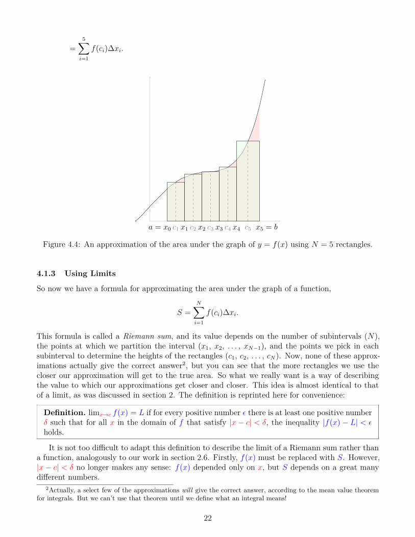
=5∑

i=1

f(ci)∆xi.

x5 = ba = x0 c1 c2 c3 c4 c5x1 x2 x3 x4

Figure 4.4: An approximation of the area under the graph of y = f(x) using N = 5 rectangles.

4.1.3 Using Limits

So now we have a formula for approximating the area under the graph of a function,

S =N∑i=1

f(ci)∆xi.

This formula is called a Riemann sum, and its value depends on the number of subintervals (N),the points at which we partition the interval (x1, x2, . . . , xN−1), and the points we pick in eachsubinterval to determine the heights of the rectangles (c1, c2, . . . , cN). Now, none of these approx-imations actually give the correct answer2, but you can see that the more rectangles we use thecloser our approximation will get to the true area. So what we really want is a way of describingthe value to which our approximations get closer and closer. This idea is almost identical to thatof a limit, as was discussed in section 2. The definition is reprinted here for convenience:

Definition. limx→c f(x) = L if for every positive number ϵ there is at least one positive numberδ such that for all x in the domain of f that satisfy |x− c| < δ, the inequality |f(x)− L| < ϵholds.

It is not too difficult to adapt this definition to describe the limit of a Riemann sum rather thana function, analogously to our work in section 2.6. Firstly, f(x) must be replaced with S. However,|x− c| < δ no longer makes any sense: f(x) depended only on x, but S depends on a great manydifferent numbers.

2Actually, a select few of the approximations will give the correct answer, according to the mean value theoremfor integrals. But we can’t use that theorem until we define what an integral means!

22

The question in the original definition was: what condition forces f(x) to approach L? Theanswer was: x must become arbitarily close to c, or |x− c| < δ. The new question is: what conditionforces S to approach L? In other words, what condition forces our rectangular approximations tobecome arbitrarily accurate? Your first instinct might be to say that the number of rectangles mustbecome arbitrarily large, or N > M , but there is a subtlety that prevents this from working.

4321

1

2

Figure 4.5: A (bad) rectangular approximation of the area under y =√x from x = 0 to x = 4 with

the property that it never becomes a good approximation no matter how many rectangles are used.

In figure 4.5, the borders of the rectangles are at the x-coordinates: 4, 2, 1, 1/2, 1/4, 1/8, . . . ,1/2n. Each evaluation point ci is the right-most point within its rectangle. You can easily see thatthe first rectangle substantially overestimates the area under the curve y =

√x, and when we add

new rectangles they are just added to the left-hand side (they do not affect the first rectangle).Therefore, that overestimation will never go away, and so S will never approach the true area underthe curve (L).

So we need a different way to specify that the rectangular approximation becomes arbitrarilyaccurate. It turns out that the best way to do this is to specify that the width of the largestrectangle becomes arbitrarily small. This will exclude the approximation in figure 4.5 because thewidth of the largest rectangle never drops below 2. If we denote the width of the largest rectangle(or, equivalently, the greatest ∆xi) as ||∆||, then we can replace |x− c| < δ (x becomes arbitrarilyclose to c) with ||∆|| < δ (||∆|| becomes arbitrarily small).

With a few other things cleaned up, we get the following definition for the limit of a Riemannsum, which I like to write as

lim||∆||→0

a→b∑i

f(ci)∆xi = L.

(The symbol∑a→b

i is just shorthand to indicate a summation∑N

i=1 where the first xi is a and thelast xi is b.)

Definition. lim||∆||→0

∑a→bi f(ci)∆xi = L if for every positive number ϵ there is at least one

positive number δ such that for all Riemann sums of f over [a, b] that satisfy ||∆|| < δ, theinequality |S − L| < ϵ holds.

And there we have our definition: if

lim||∆||→0

a→b∑i

f(ci)∆xi = L,

then ∫ b

a

f(x) dx = L.

23

4.1.4 Implications

Unfortunately, this definition of the integral does not give us a simple way to actually find its value,but it rather gives us an extraordinarily difficult limit to try to guess and then subsequently proveformally. Luckily, there are two facts that make it possible to sidestep the limit definition somewhat:

• For continuous, positive functions, the integral corresponds to the area under the curve. Thisis simply a consequence of the fact that we derived our definition from finding the area undera function’s graph. For example,

∫ 1

−1

√1− x2 dx = π/2 because the area under the graph is

a semicircle of radius 1.

• There is a theorem stating that if f is continuous on [a, b], then the limit in our definitionof

∫ b

af(x) dx exists. This should make intuitive sense – all it is saying is that any smooth

(continuous) curve can be approximated as well as you might want using rectangles.

The second fact may not seem very important, but it is the key to evaluating integrals. Why?If your function is continuous, then the theorem tells you that the integral for its integral exists(which is very hard to prove in general) – all you have to do is find the actual value (which is usuallymuch easier).

To see how to use the limit definition to evaluate an integral, consider∫ 1

0

x dx.

Now consider the Riemann sum consisting of N rectangles of equal widths (since the total intervalhas width 1, each rectangle has a width of 1/N) and with each point of evaluation being at the farright edge of its rectangle. Then rectangle i is bounded on the left by x = (i−1)(1/N) and boundedon the right by i/N . This means that xi = ci = i/N , and ∆xi = xi−xi−1 = i/N− (i−1)/N = 1/N .We can then directly find the value of this Riemann sum:

Sn =N∑i=1

f(ci)∆xi =N∑i=1

f

(i

N

)[1

N

]=

N∑i=1

i

N2=

1

N2

N∑i=1

i =1

N2

(N(N + 1)

2

)=

N + 1

2N=

1

2+

1

2N

Now, since f(x) = x is continuous, we know that lim||∆||→0

∑a→bi f(ci)∆xi exists. What does

this mean? According to the definition, it means that S gets arbitrarily close to L as ||∆|| getsarbitrarily close to 0. But wait: we already have a sequence of Riemann sums for which ||∆|| getsarbitrarily close to 0: the sums we computed above, for which ||∆|| = ∆xi = 1/N since all of therectangles are of the same width. Clearly, as N approaches ∞, ||∆|| = 1/N will approach 0. So Sn

must get arbitrarily close to L as N gets approaches ∞; in other words,

limN→∞

Sn = L = lim||∆||→0

a→b∑i

f(ci)∆xi =

∫ 1

0

x dx.

We have reduced the extremely complicated limit on the right to the comparatively trivial limit onthe left, which is easily evaluated:

limN→∞

Sn = limN→∞

[1

2+

1

2N

]=

1

2.

24

Consequently, ∫ 1

0

x dx =1

2.

Of course, you could also evaluate this integral by noting that it represents a triangle with bothbase and height of 1. Geometrically, the quantity 1/2 + 1/2N represents the area of the triangleplus the overestimation accrued by using rectangles, which decreases as the number of rectanglesN increases.

But you probably use the fundamental theorem of calculus to evaluate integrals, so why botherwith all these details about Riemann sums? Well, in fact, the formal definition of the integral showsup in the proof of the fundamental theorem of calculus! See section 4.2.3 for details on this.

4.2 The First Fundamental Theorem of CalculusPrerequisite Knowledge. Know what the symbols in the fundamental theorem of calculusmean, and understand the mean value theorem.

4.2.1 The Form of the Equation

The fundamental theorem of calculus states that when the derivative of a function is integrated,the result is the original function evaluated at the bounds of integration. In other words,∫ b

a

f ′(x) dx = f(b)− f(a).

Of course, if the function f(x) is G(x), an antiderivative of g(x), then f ′(x) = G′(x) = g(x) and weget the more familiar result that ∫ b

a

g(x) dx = G(b)−G(a).

However, when trying to understand the theorem intuitively, the first form is more useful. (It isdifficult to visualize an antiderivative.)

4.2.2 The Main Idea ∫ b

a

slope dx = change in y

When slope (change in y per change in x) is multiplied by dx, a small change in x, we get dy, asmall change in y. Since

∫ b

ameans “add a lot of, from a to b”, when it is applied to dy we get ∆y,

a large change in y (from a to b).This is the fundamental idea of the theorem, but there is also a third component to keep in

mind, which is that the left side of this equation also corresponds to the area under the graph of“slope” (also known as f ′). This is because “slope”, at any given point, is the distance straightup from the x-axis to the graph of “slope”, and dx is a small width. When we multiply these twonumbers together, we get the area of a very thin rectangle extending from the x-axis to the graphof “slope”. This rectangle is a great approximation of the area under the graph in the small intervalrepresented by dx. When we apply

∫ b

a(add a lot of, from a to b) to the areas under the graph over

small intervals, we get the total area under the graph in the whole interval (from a to b).

25

4.2.3 The Details

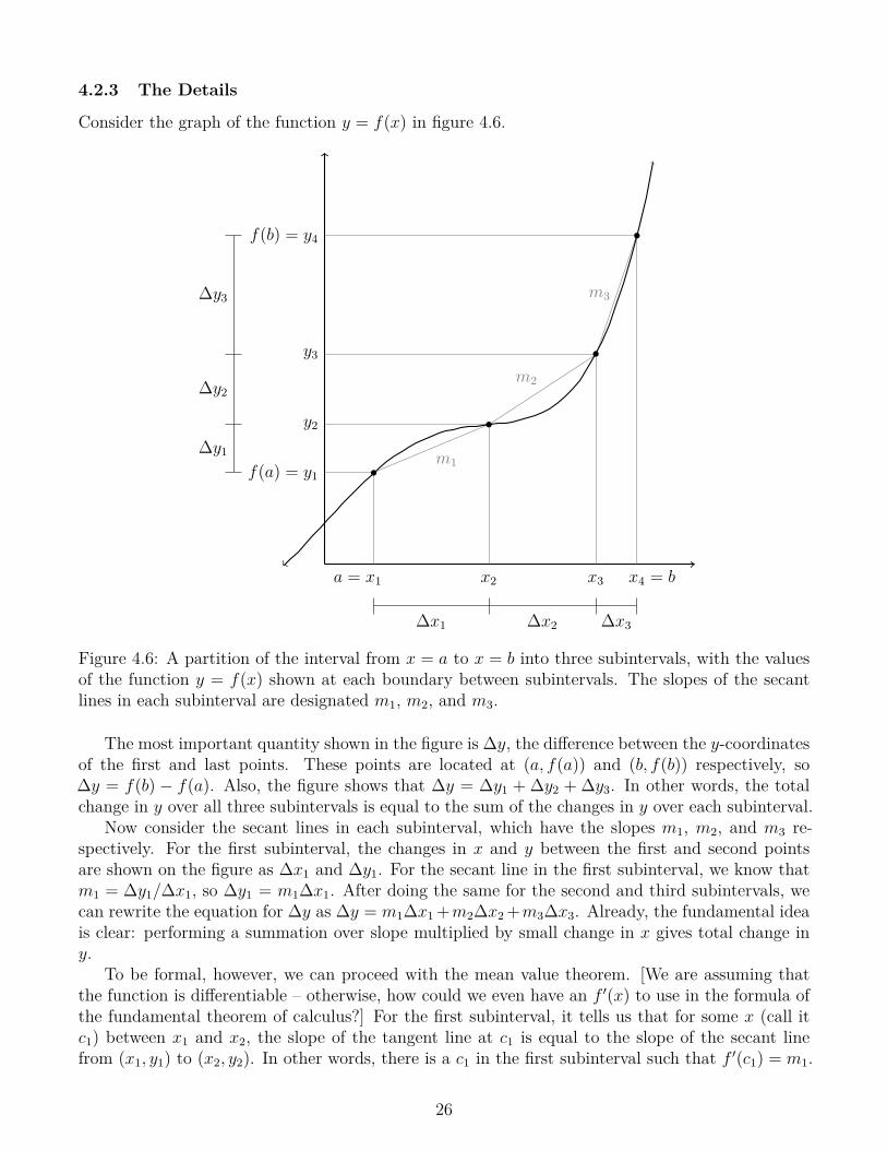
Consider the graph of the function y = f(x) in figure 4.6.

m1

m2

m3

a = x1

f(a) = y1

x2

y2

x3

y3

x4 = b

f(b) = y4

∆x1 ∆x2 ∆x3

∆y1

∆y2

∆y3

Figure 4.6: A partition of the interval from x = a to x = b into three subintervals, with the valuesof the function y = f(x) shown at each boundary between subintervals. The slopes of the secantlines in each subinterval are designated m1, m2, and m3.

The most important quantity shown in the figure is ∆y, the difference between the y-coordinatesof the first and last points. These points are located at (a, f(a)) and (b, f(b)) respectively, so∆y = f(b) − f(a). Also, the figure shows that ∆y = ∆y1 + ∆y2 + ∆y3. In other words, the totalchange in y over all three subintervals is equal to the sum of the changes in y over each subinterval.

Now consider the secant lines in each subinterval, which have the slopes m1, m2, and m3 re-spectively. For the first subinterval, the changes in x and y between the first and second pointsare shown on the figure as ∆x1 and ∆y1. For the secant line in the first subinterval, we know thatm1 = ∆y1/∆x1, so ∆y1 = m1∆x1. After doing the same for the second and third subintervals, wecan rewrite the equation for ∆y as ∆y = m1∆x1+m2∆x2+m3∆x3. Already, the fundamental ideais clear: performing a summation over slope multiplied by small change in x gives total change iny.

To be formal, however, we can proceed with the mean value theorem. [We are assuming thatthe function is differentiable – otherwise, how could we even have an f ′(x) to use in the formula ofthe fundamental theorem of calculus?] For the first subinterval, it tells us that for some x (call itc1) between x1 and x2, the slope of the tangent line at c1 is equal to the slope of the secant linefrom (x1, y1) to (x2, y2). In other words, there is a c1 in the first subinterval such that f ′(c1) = m1.

26

Since the mean value theorem applies just as well to each other subinterval, we also have a c2 inthe second subinterval and a c3 in the third subinterval such that f ′(c2) = m2 and f ′(c3) = m3. Wecan then rewrite the equation for ∆y again as ∆y = f ′(c1)∆x1 + f ′(c2)∆x2 + f ′(c3)∆x3. Since thisequation has quite a bit of repetition, we can also write it as a summation:

∆y =3∑

i=1

f ′(ci)∆xi.

Recall from earlier that ∆y = f(b)− f(a). Also, the equation we found is true for any numberof subintervals, not just 3. If we let N be the number of subintervals, then we get

f(b)− f(a) =N∑i=1

f ′(ci)∆xi.

Really, this equation is the fundamental theorem of calculus, except that it is for a finite numberof subintervals instead of an infinite number. If we take the limit of both sides as the number ofsubintervals approaches infinity,

limN→∞

[f(b)− f(a)] = limN→∞

N∑i=1

f ′(ci)∆xi,

then the left side stays the same (it does not depend upon the number of subintervals), while theright side is exactly the definition of an integral.3 Therefore, we have

f(b)− f(a) =

∫ b

a

f ′(x) dx.

4.2.4 Alternate Proof

Prerequisite Knowledge. Understand Euler’s method.

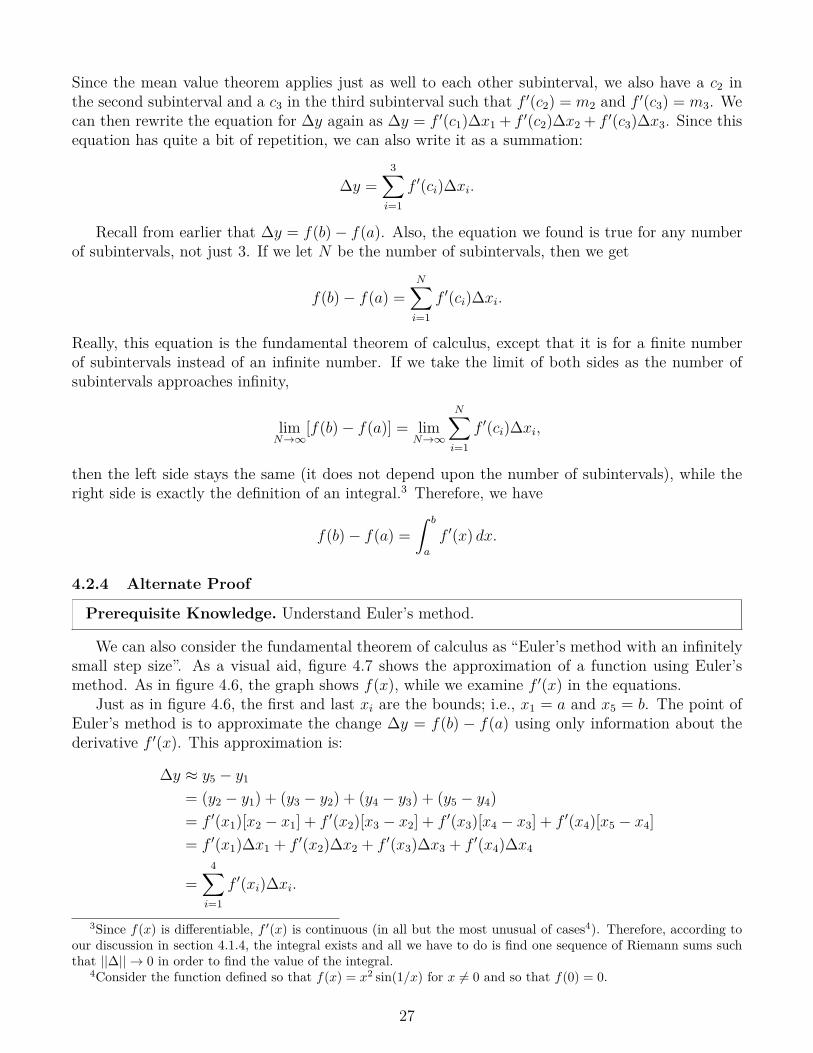
We can also consider the fundamental theorem of calculus as “Euler’s method with an infinitelysmall step size”. As a visual aid, figure 4.7 shows the approximation of a function using Euler’smethod. As in figure 4.6, the graph shows f(x), while we examine f ′(x) in the equations.

Just as in figure 4.6, the first and last xi are the bounds; i.e., x1 = a and x5 = b. The point ofEuler’s method is to approximate the change ∆y = f(b) − f(a) using only information about thederivative f ′(x). This approximation is:

∆y ≈ y5 − y1

= (y2 − y1) + (y3 − y2) + (y4 − y3) + (y5 − y4)

= f ′(x1)[x2 − x1] + f ′(x2)[x3 − x2] + f ′(x3)[x4 − x3] + f ′(x4)[x5 − x4]

= f ′(x1)∆x1 + f ′(x2)∆x2 + f ′(x3)∆x3 + f ′(x4)∆x4

=4∑

i=1

f ′(xi)∆xi.

3Since f(x) is differentiable, f ′(x) is continuous (in all but the most unusual of cases4). Therefore, according toour discussion in section 4.1.4, the integral exists and all we have to do is find one sequence of Riemann sums suchthat ||∆|| → 0 in order to find the value of the integral.

4Consider the function defined so that f(x) = x2 sin(1/x) for x ̸= 0 and so that f(0) = 0.

27

y1

x1

y2

x2

y3

x3

y4

x4

y5

x5

Figure 4.7: Euler’s method, using the same naming conventions as figure 4.6. The graph of y = f(x)is shown, and Euler’s method is applied to the derivative f ′(x) in order to find the slope of eachline segment.

Now, Euler’s method would be no good if its approximation did not get better and better as weused more and more steps. So, as a reminder, we have

f(b)− f(a) ≈N∑i=1

f ′(xi)∆xi

for any finite number of steps N . However, if we take the limit as N → ∞, then the approximationwill become correct and we find once again that

f(b)− f(a) = limN→∞

N∑i=1

f ′(xi)∆xi =

∫ b

a

f ′(x) dx.

Note that once again, the key idea is multiplying slope f ′(x) by change in x to get change in y, andthen summing all of those small changes in y to get the total f(b)− f(a).

Really, numerical approximation of an integral using a left Riemann sum and numerical ap-proximation of a differential equation using Euler’s method are exactly the same thing (just withdifferent names and different intended uses). This can also be seen by the fact that the way to solvethe differential equation

dy

dx= f ′(x)

is to integrate both sides with respect to x – thus intimately relating the solutions of integrals andfirst-order differential equations.

4.2.5 Conclusion ∫ b

a

f ′(x) dx =

∫ b

a

dy

dxdx =

∫ f(b)

f(a)

dy = f(b)− f(a).

28

4.3 The Second Fundamental Theorem of CalculusPrerequisite Knowledge. Know what the symbols in the second fundamental theorem ofcalculus mean.

The second fundamental theorem of calculus is often presented as

d

dx

∫ x

a

f(t) dt = f(x).

However, the important idea is that you are finding the rate of change of the value of the integralwith respect to its upper bound. We can relabel some variables to make this more clear:

d

db

∫ b

a

f(x) dx = f(b).

Now consider the meaning of the various symbols in the formula. Firstly,∫ b

af(x) dx is the area

under the graph of y = f(x) from x = a to x = b. d/db signifies rate of change with respect to b. Inthis case, the left side of the formula is the rate of change of the area with respect to its right-handbound. Mathematically, this means

∆[area]∆b

=[area from a to (b+∆b)]− [area from a to b]

∆b=

[area from b to (b+∆b)]

∆b.

If ∆b is small, then the value of the function will not change significantly over the interval [b, b+∆b],but will remain approximately f(b). The area under the curve is then approximately a rectanglewith height f(b) and width ∆b, with area f(b)∆b. We then have

d

db

∫ b

a

f(x) dx =∆[area]∆b

=f(b)∆b

∆b= f(b).

Another (less intuitive) way of proving the second fundamental theorem of calculus is to use thefirst fundamental theorem of calculus,∫ b

a

f(x) dx = F (b)− F (a).

If we differentiate both sides of this equation with respect to b, F (b) will become F ′(b) = f(b), whileF (a) will be a constant. Therefore, we have

d

db

∫ b

a

f(x) dx =d

db

[F (b)− F (a)

]= f(b).

5 Sequences and SeriesFormal proofs can be given for each of the theorems in this section. They are not given here, andinstead each theorem is accompanied by an explanation of why the result makes sense. This, Ibelieve, is far more helpful, especially in remembering all of the conditions that are associated withthe various theorems. (If you know, intuitively, why a theorem is true, then it is always easy torecall what its conditions are.)

Also, in this section I often refer to the “vergence” of a series or integral. This means the factof its converging or diverging, as in: the two series have the same vergence; this diagram helps youunderstand the vergence of the series; we can determine the integral’s vergence.

29

5.1 Bounded Monotonic Sequences

Prerequisite Knowledge. Know what a sequence is and what notation is used for sequences.

"This section discusses sequences, not series.

Suppose we have a sequence an, and that we know two things about it: (1) its terms neverdecrease, and (2) its terms never become greater than a certain number (call it M , for maximum).The graph of such a sequence is depicted in figure 5.1.

1 2 3 4 5 6 7 8 9 100

1

2

3

4

n

an

Figure 5.1: A nondecreasing sequence that is bounded above. No term in the sequence is greaterthan 4, including the ones not shown on the graph. This sequence happens to be an = 4 −3 exp(−n/4).

It is reasonable to conclude that this sequence would have to converge, because it cannot divergein any of the usual ways sequences diverge. It cannot diverge by decreasing without bound (becauseit is nondecreasing), it cannot diverge by increasing without bound (because it is bounded above),and it cannot diverge by oscillating (because it is nondecreasing and oscillations require both increaseand decrease).

To be precise, the number M which is greater than all terms in the sequence is called an upperbound. Of course, there are (infinitely) many upper bounds for a sequence that is bounded above.For the sequence in figure 5.1, for instance, both 4 and 5 are upper bounds. However, 4 is moreinteresting because it is the least upper bound: any number less than 4 will no longer be an upperbound. In fact, according to a property of the real numbers called completeness, any sequence thathas an upper bound also has a least upper bound.

You can use this fact to conclude that a nondecreasing sequence bounded above converges.Firstly, you know that the sequence will get arbitrarily close to its least upper bound (call it L, forleast). If it did not, then there would be some difference between L and the highest the sequencereaches, which would mean that an upper bound smaller than L would exist. This would contradictthe fact that L is the least upper bound. You also know that the sequence can only get closer toL, not farther away, because it is nondecreasing. Since the sequence gets arbitrarily close to L anddoes not ever get farther away from L, clearly its limit must be L. (What a coincidental choice ofvariable name!) Since the sequence has a limit, it converges.

We saw that a nondecreasing sequence bounded above must converge, and, analogously, a non-increasing sequence bounded below must also converge. Therefore, we know that:

30

Theorem 1. If a sequence is nondecreasing and bounded above, or it is nonincreasing andbounded below, then it converges.

Since bounded means “both bounded above and bounded below”, and since monotonic means“either nonincreasing or nondecreasing”, the above theorem also implies that all bounded monotonicsequences converge, which is the result typically presented in textbooks.

5.2 The Integral Test and Remainder Formula

Prerequisite Knowledge. Understand what improper integrals and infinite series look likegraphically.

n

y

1 2 3 4 5 6 7 8 9

Figure 5.2: The graph of a function y = f(n) to which the integral test may be applied. Thearea under the curve is overestimated by the light gray rectangles (a left-hand approximation) andunderestimated by the dark gray rectangles (a right-hand approximation). Only eight rectanglesare shown, but there are (infinitely) more to the right.

An infinite series and an improper integral are really quite similar. Both relate to areas on thegraph of a function, as shown in figure 5.2. In the figure, the area of the light gray rectangle witha left side at x = n is f(n), and the area of the dark gray rectangle with a left side at x = n isf(n+ 1). Therefore, the sum of the areas of the light gray rectangles is

∞∑n=1

f(n),

and the sum of the dark gray rectangles is∞∑n=1

f(n+ 1) =∞∑n=2

f(n).

Since the area under the curve (right of x = 1) is less than the area of the light gray rectangles butgreater than the area of the dark gray rectangles, we can write the inequality

∞∑n=2

f(n) ≤∫ ∞

1

f(n) dn ≤∞∑n=1

f(n).

31

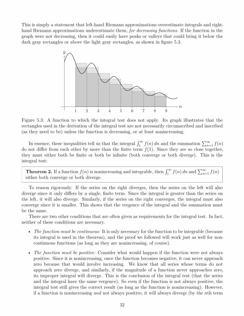
This is simply a statement that left-hand Riemann approximations overestimate integrals and right-hand Riemann approximations underestimate them, for decreasing functions. If the function in thegraph were not decreasing, then it could easily have peaks or valleys that could bring it below thedark gray rectangles or above the light gray rectangles, as shown in figure 5.3.

n

y

1 2 3 4 5 6 7 8 9

Figure 5.3: A function to which the integral test does not apply. Its graph illustrates that therectangles used in the derivation of the integral test are not necessarily circumscribed and inscribed(as they need to be) unless the function is decreasing, or at least nonincreasing.

In essence, these inequalities tell us that the integral∫∞1

f(n) dn and the summation∑∞

n=1 f(n)do not differ from each other by more than the finite term f(1). Since they are so close together,they must either both be finite or both be infinite (both converge or both diverge). This is theintegral test:

Theorem 2. If a function f(n) is nonincreasing and integrable, then∫∞1

f(n) dn and∑∞

n=1 f(n)either both converge or both diverge.

To reason rigorously: If the series on the right diverges, then the series on the left will alsodiverge since it only differs by a single, finite term. Since the integral is greater than the series onthe left, it will also diverge. Similarly, if the series on the right converges, the integral must alsoconverge since it is smaller. This shows that the vergence of the integral and the summation mustbe the same.

There are two other conditions that are often given as requirements for the integral test. In fact,neither of these conditions are necessary.

• The function must be continuous: It is only necessary for the function to be integrable (becauseits integral is used in the theorem), and the proof we followed will work just as well for non-continuous functions (as long as they are nonincreasing, of course).

• The function must be positive: Consider what would happen if the function were not alwayspositive. Since it is nonincreasing, once the function becomes negative, it can never approachzero because that would involve increasing. We know that all series whose terms do notapproach zero diverge, and similarly, if the magnitude of a function never approaches zero,its improper integral will diverge. This is the conclusion of the integral test (that the seriesand the integral have the same vergence). So even if the function is not always positive, theintegral test still gives the correct result (as long as the function is nonincreasing). However,if a function is nonincreasing and not always positive, it will always diverge (by the nth term

32

test). It is therefore rather pointless to apply the integral test. (However, there’s still nopoint in adding one more condition to remember if it’s not even necessary: that just addsconfusion!)

Since improper integrals are typically easier to evaluate than infinite series, the inequality of theintegral test (reprinted here for convenience)

∞∑n=2

f(n) ≤∫ ∞

1

f(n) dn ≤∞∑n=1

f(n)

also gives us a nice approximation for nonincreasing infinite series. From the two right-hand terms,we have ∫ ∞

1

f(n) dn ≤∞∑n=1

f(n),

and we can add f(1) to each of the two left-hand terms to get∞∑n=1

f(n) ≤ f(1) +

∫ ∞

1

f(n) dn.

Combining these two inequalities, we have that∫ ∞

1

f(n) dn ≤∞∑n=1

f(n) ≤ f(1) +

∫ ∞

1

f(n) dn.

However, this only bounds the summation within an interval of width f(1). To get a better approx-imation, we can re-write the integral test inequality, except placing the first rectangle at n = Ninstead of n = 1:

∞∑n=N+1

f(n) ≤∫ ∞

N

f(n) dn ≤∞∑

n=N

f(n).

Now, following the same steps as before except adding f(N) instead of f(1) to get the inequalityon the left-hand side, we have∫ ∞

N

f(n) dn ≤∞∑

n=N

f(n) ≤ f(N) +

∫ ∞

N

f(n) dn.

This bounds part of the series within an interval of width f(N). Of course, since the function isdecreasing, this is a smaller interval than before, which makes a better approximation. To get abound for the entire summation, just add

∑N−1n=1 f(n) to all three terms. We then find the integral

test error bound:

Theorem 3. For any nonincreasing, integrable function f and positive integer N ,

N∑n=1

f(n) +

∫ ∞

N

f(n) dn ≤∞∑n=1

f(n) ≤N−1∑n=1

f(n) +

∫ ∞

N

f(n) dn.

This inequality allows you to add a finite number of terms of a series and compute an integral,then use these numbers to place a bound on the value of a nonincreasing series (of which presumablyyou cannot find the exact value).

33

5.3 The Limit Comparison Test

Prerequisite Knowledge. Understand limits and series intuitively, and be able to evaluatelimits of simple quotients.

Suppose we have two series, an and bn, such that

limn→∞

anbn

= C,

where C is a nonzero but finite number. For now, suppose that every term of both series is positive.(We will consider otherwise later.) What this limit says is that

anbn

≈ C (for sufficiently large n),

or equivalentlyan ≈ bn · C (for sufficiently large n).

Now, if we have a convergent series and multiply it by a finite number, it will remain convergent;similarly, if we have a divergent series and multiply it by a finite number, it will remain divergent –as long as the number is nonzero, of course! So it follows directly that if an/bn = C for all n, thenthe series must have the same vergence. The limit comparison test is simply an extension for thecase that this equation is not exactly true, but is approximately true for large n. We can disregardsmall n, because any finite number of terms of a series will only sum to a finite number, and thiscannot affect the vergence of a series. This gives us:

Theorem 4. If limn→∞ an/bn = C, where is C is finite and nonzero, and an and bn are bothpositive for all (or at least all sufficiently large) n, then an and bn either both converge or bothdiverge.

Naturally, the next question is: why must all of the terms of both series be positive? The issue isa subtlety with conditionally convergent series. More specifically, we can form two series as follows:

an = [large but convergent series] + [small but divergent series]

andbn = [large but convergent series].

Clearly, an is divergent and bn is convergent due to the way series add, so it would be a big problemif the limit comparison test were to apply to this pair of series. (That is, it would be a problem iflimn→∞ an/bn were finite and nonzero.) Now, your first thought might be for the large series to be,for instance, 1000/n2 and for the small series to be 1/n. However, the limit is

limn→∞

1000/n2 + 1/n

1000/n2= ∞

because 1/n eventually becomes larger than 1000/n2. (You should verify both parts of this statementyourself.) This is not unexpected – after all, 1/n is divergent, while 1000/n2 is convergent. In fact,this would always happen if it were not for alternating series. Recall that the only condition forconvergence of an alternating series is that its terms decrease to zero (see section 5.4), which isfar less stringent than the condition for convergence of a general series. For instance, (−1)n/

√n is

34

convergent, and is also larger than the divergent 1/n in the limit. (Check this.) The key is thatnegative terms allow convergent series to be larger than divergent series in the limit. For this pairof series, we have

limn→∞

(−1)n/√n+ 1/n

(−1)n/√n

= 1.

(You should also verify this limit.) This would contradict the conclusion of the limit comparisontest because the series in the numerator and denominator have different vergence. So, due to thefact that conditionally convergent series can outweigh divergent series in the limit, we must eitherdiscard the idea of testing vergence by comparing the magnitudes of terms or discard series withnegative terms from the limit comparison test. (Most people choose the latter.)

5.4 The Alternating Series Test and Remainder Formula

Prerequisite Knowledge. Understand series and their notation.

An example of an alternating series is∑∞

n=1(−1)n+1an, where an is always positive. The bestway to understand the vergence of this series is to draw a diagram such as figure 5.4.

S

n

1

2

3

4

5

6

S1

S2

S3

S4

S5

S6

a1

a2

a3

a4

a5

a6

a7

Figure 5.4: An alternating series is a sequence of additions and subtractions, which can be visualizedas movements left and right on a number line. The terms of the series (an) are the sizes of themovements, and the partial sums (Sn) are the results of consecutive movements. The series depictedhas the terms an = (−1)n+1/n.

The figure makes it quite apparent that the series it depicts converges. The partial sums alwayshave a left bound and a right bound. The left bound starts at 0 and then changes to S2, S4, S6,and so on. The right bound starts at S1, then changes to S3, S5, and so on. At any given point(i.e., vertical position on the diagram), all future partial sums are between the two current bounds.Furthermore, both bounds continue to move toward each other. If the distance between the boundsshrinks to zero as n increases without bound, then surely the series must converge, because thesequence of partial sums would have to converge to the meeting point of the left and right bounds.(This is the squeeze theorem, sort of.)

35

What we would like to do now is devise precise conditions that a series must obey such that thediscussion above is applicable and thus that the series converges.

1. The bounds must always be moving toward one another as n increases. We can see in thefigure that the right bound, for instance, always moves to the left. For instance, S3 is fartherto the left than S1. This is because the change from S1 to S3 is negative, which is only truebecause a2 (a move to the left) is greater than a3 (a move to the right). Similarly, the leftbound will only continue to move to the right if a4 is less than a3, a6 is less than a5, and soon. This gives us the condition that the sequence of terms an must be decreasing (or at leastnonincreasing).

2. Also, the distance between the bounds must eventually converge to zero. Since at any givenpoint the distance between the bounds is equal to a term of the series, this condition isequivalent to the condition that limn→∞ an = 0.

From this, we get:

Theorem 5. If the magnitudes of the terms of an alternating series are nonincreasing, andtheir limiting value is zero, then the series converges.

Figure 5.4 also illustrates an interesting and very useful property of alternating series. Supposewe have calculated the the fourth partial sum, S4, and want to use it to estimate the sum of theentire series. For a general series, there is no way to know how good this approximation is. However,alternating series have left and right bounds on their partial sums, as we used in the “proof” ofthe theorem above. In particular, we know that all partial sums Sn lie between S4 and S5, wheren > 5. This means that the sum S of the entire series must also lie between S4 and S5. So if weestimate S by S4, then the error cannot be more than the distance between S4 and S5, which is a5.Symbolically, the error in estimating S by S4 is |S − S4|, and so we have that |S − S4| ≤ a5. Thissame reasoning will apply for any Sn, and so we find that:

Theorem 6. For any alternating series whose terms decrease in magnitude monotonically tozero, |S − Sn| ≤ an+1.

5.5 The Ratio and Root TestsPrerequisite Knowledge. Understand the geometric series test and the direct comparisontest.

The principal idea of the ratio and root tests is to classify a series’ vergence based on how fast itdecreases (or increases). For a general series

∑∞n=1 an, both |an+1/an| and n

√|an| give quantitative

measures of its rate of decrease (for which they are less than 1) or increase (for which they aregreater than 1). We will discuss the ratio test first, using figure 5.5 to see graphically how a series’common ratio affects its convergence or divergence. Take a moment now to study the figure (onpage 37). It is complex, and so we will discuss each aspect of it in detail.

Perhaps the easiest series to analyze are geometric series, which have a constant common ratio.For the geometric series

∑∞n=0 ar

n, convergence occurs for |r| < 1 and divergence occurs for |r| ≥ 1(according to the geometric series test). Three geometric series are shown in figure 5.5: those withterms (1/4)n, 1, and (3/2)n. The common ratios of these series are 1/4, 1, and 3/2 respectively;since these are constants, they appear as horizontal lines when plotted as functions of n. All

36

1/n! ∼ 1/(n+ 1)

(1/4)n ∼ 1/4

n/2n ∼ 12(

n+1n )

(3/4)n/n ∼ 34(

nn+1)

1/n2 ∼ ( nn+1)

2

1/n ∼ ( nn+1) 1 ∼ 1

n ∼ (n+1n )

(3/2)n ∼ 3/2

n! ∼ n+ 1

1 2 3 4 5 6 7 8 9 100

1/2

1

n

R

Figure 5.5: The common ratios R of several series plotted as functions of n. Each plot is labeled withthe nth term of its series (an) and, after the tilde (∼), the series’ common ratio (Rn = an+1/an). Theratio test can be used to show that all the series in green converge and all the series in red diverge;the test cannot be applied to any of the series in orange. The boundary between convergence anddivergence is shown in black. The series corresponding to the sinusoid, which is not labeled on thediagram due to its size, is

∑∞n=1

∏nk=1[0.95+

110sin k], and its common ratio is 0.95+ 1

10sinn. (Note:

the slope of the n! series has been reduced so that it does not leave the page.)

37

geometric series may be placed on figure 5.5. If they were, there would be a block of solid greenbelow R = 1 and a block of solid red above R = 1, with the series

∑∞n=1 1 acting as the boundary.

Notice that the other series in the diagram follow a similar pattern: ones mostly below R = 1 areconvergent and ones mostly above R = 1 are divergent, with a few exceptions.

Of course, there are also geometric (and other) series with negative common ratios, and theseare dealt with the same way as series with positive common ratios: figure 5.5 and its coloring arecompletely symmetric with respect to the n-axis because the geometric series test depends on |r|,not r.

Now let us turn to the non-geometric convergent series in figure 5.5. First consider the one withterms 1/n!. Past n = 3, its common ratio is less than that of the convergent geometric series (1/4)n.This means that we can construct another geometric series whose fourth term is equal to the fourthterm of 1/n! and whose common ratio is equal to that of (1/4)n. We can call this series gn. If you’rein the market for a precise formula, it is gn = (1/4!)(1/4)n−4. Since the common ratio (R) of 1/n!is less than that of gn at n = 4, and since a5 = a4 ×R4 for both series, we know that the fifth termof 1/n! is less than that of gn. And since the common ratio of 1/n! continues to be less than thatof gn for all n > 4, we can conclude that all terms of 1/n! are less than the corresponding terms ofgn. According to the direct comparison test, this means that 1/n! is convergent.

So what? Isn’t it obvious, one might ask, that 1/n! converges? Perhaps yes, but our argumentabove using the common ratios of a given, non-geometric series and a different, geometric seriescan be extended easily. In figure 5.5, the argument translates to: given an arbitrary series, plot itscommon ratio as a function of n. If we can draw a horizontal line below R = 1 (corresponding toa convergent geometric series) such that at some point the graph of the series’ common ratio dipspermanently below the horizontal line (corresponding to the series’ terms becoming permanentlysmaller than the convergent geometric series), then we can conclude that the series is convergent.

Now take a moment to consider the two other convergent series in figure 5.5. Can you usethe reasoning above to conclude that they are convergent, even though their common ratios donot decrease to zero like that of 1/n!? [You can check the horizontal asymptotes of the graphs byreading the equations for the common ratios, which are labeled on each graph to the right of thetilde (∼).]

The divergent series in figure 5.5 can be analyzed in a similar fashion to the convergent ones.You can always use the divergent geometric series with terms an = 1 and common ratio R = 1: ifa series’ common ratio is always larger than 1, then by the direct comparison test it must diverge.(Can you see how to construct a rigorous argument as we did above?)

What about the series in orange? Do they converge or diverge? Consider those with terms 1/nand 1/n2. For either series, can we draw a horizontal line below R = 1 but also above the series’graph? It may look like we can, but if you check the formulae for each on the graph, you can seethat limn→∞Rn = 1 for both. In other words, both series get arbitrarily close to R = 1, and soit is impossible to show that they converge by drawing a line that is strictly between them andR = 1. Since both series’ graphs are entirely below R = 1, we also cannot show that they divergeby showing that they are above R = 1. So we cannot apply the reasoning shown above to eitherseries. In fact, 1/n diverges and 1/n2 converges. So there is still a border between the convergentand divergent series we can identify using common ratios, where some series converge and someseries diverge without any apparent pattern.

The sinusoid is a third example of a series whose vergence cannot be determined by comparisonwith geometric series. Clearly it passes above any line below R = 1, but it also passes below anyline above R = 1. Therefore we cannot compare it to a geometric series using common ratios. (Thisseries converges.)

38

Hopefully, the intuitive idea of determining series’ vergence by their common ratios is nownatural to you. We will now translate our criteria above into an easier-to-work-with definition. Wehave two criteria:

1. Rn is greater than 1 for all sufficiently large n. This is equivalent to the statement limn→∞ Rn >1.5 (Think about this until you are convinced. You can check that the two statementsare equivalent for each of the divergent series in figure 5.5.) From this, we have that iflimn→∞(an+1/an) > 1, then

∑an diverges.

2. There is a number L, less than 1, such that Rn is less than L for all sufficiently large n. Thisis equivalent to the statement limn→∞ Rn < 1. [Also convince yourself of this. You can checkthe equivalence of the statements for both the convergent (where they are both true) andambiguous (where they are both false) series labeled in the figure.] From this, we have thatif limn→∞(an+1/an) < 1, then

∑an converges.

Since, as we mentioned earlier, all of this reasoning is symmetric with respect to the n-axis (onlyseries with positive common ratios were discussed for the sake of brevity), we should really replacean+1/an with |an+1/an| to be more general. Thus, we obtain what is commonly known as the ratiotest:

Theorem 7. Let L = limn→∞ |an+1/an|. If L > 1, then∑∞

n=1 an diverges; and if L < 1, then∑∞n=1 an converges. If L = 1 or the limit does not exist, then no conclusion can be drawn.

On a broad scale, let’s summarize what we have done. We have identified a property,

Rn =

∣∣∣∣an+1

an

∣∣∣∣ ,which is constant for geometric series (Rn = |r| for

∑rn) and can be used to determine the

vergence of those series: (Rn < 1 means convergence; Rn ≥ 1 means divergence), then extended itto other series in the limit, except with the boundary line being ambiguous: limn→∞Rn < 1 meansconvergence, limn→∞ Rn > 1 means divergence, and limn→∞ Rn = 1 is inconclusive.

There is, in fact, another property R′n which is also constant and equal to |r| for geometric series∑

rn. It is n√|an|. We could go through a rigorous proof, but what is the fun in that? We can

instead simply note that our new value R′n has the same property for geometric series as R did, and

realize that it will probably naturally generalize in the same way (it does): that is, limn→∞R′n < 1

means convergence, limn→∞R′n > 1 means divergence, and limn→∞ R′

n = 1 is inconclusive. Thus,we have the root test:

Theorem 8. Let L = limn→∞n√|an|. If L > 1, then

∑∞n=1 an diverges; and if L < 1, then∑∞

n=1 an converges. If L = 1 or the limit does not exist, then no conclusion can be drawn.

As an addendum, here are four useful limits which make it much easier to apply the root testto a wide class of functions:

limn→∞

n√C = 1,

5Technically, this is not quite true. In some cases, the first statement can be true even though the limit doesnot exist, such as if Rn = 1

3 (1 + sinn). However, if the limit exists, the first statement always has to be true.To make the two statements equivalent, we would need to use a limit inferior instead of a regular limit. Seehttps://en.wikipedia.org/wiki/Limit_inferior for details if you are willing to venture out into that untamedwilderness.

39

limn→∞

n√n = 1,

limn→∞

n√n! = ∞,

andlimn→∞

n√n!

n=

1

e.

The first two limits may be proven rather easily using logarithms, and proofs of the last two can befound at http://matharticles.com/ma/ma050.pdf.

6 Vector Analysis

6.1 The GradientPrerequisite Knowledge. Understand the idea of scalar and vector fields in two and threedimensions, approximating a function with its tangent plane, partial and directional derivatives,and projections of vectors.

6.1.1 Intuition

The gradient is an operation that takes a scalar field f and returns a vector field, grad f . Thebest way to understand the gradient is to look at a diagram such as figure 6.1, which shows atwo-dimensional scalar field and its gradient.

The gradient at a particular point is a vector pointing in the direction of greatest increase andwith a magnitude equal to that rate of greatest increase. It should make sense that this idea is stillperfectly valid in three dimensions even though figure 6.1 only shows a gradient in two dimensions.

6.1.2 Definition

It turns out that the gradient and directional derivatives of a function are intimately related. Infact, given just the gradient at a single point, you can work out all of the directional derivatives atthat point! How, you ask?

Let’s work with a function of two variables. To make things simpler, instead of looking directlyat the three-dimensional graph of this function z = f(x, y), let’s just work with its tangent plane(which will exist if and only if the function is differentiable). Just as the derivative of a function isthe same as the slope of its tangent line, the directional derivative of a function is the same as theslope of its tangent line in the same direction. This tangent line will, of course, be contained withinthe tangent plane. In figure 6.3, the blue plane is the tangent plane to a function at the indicatedpoint. Figure 6.3 also shows several tangent lines to the same function, and the slope of each oneis equal to the directional derivative in the direction of the tangent line.

In particular, the slope of the vector marked “direction of greatest increase” is equal to the great-est possible directional derivative, the slope of the vector marked “direction of greatest decrease” isequal to the least possible directional derivative, the slope of the vector marked “direction of zeroincrease” is (of course) zero, and the slope of the vector marked “arbitrary direction” is somewherein between.

40

Figure 6.1: The graph of a two-dimensional scalar field, where red areas have large values and blueareas have small values. The gradient of this field is overlaid as a grid of arrows. At each pointin the field, the gradient is in the direction of greatest increase, and it is larger when that rate ofincrease is faster. See figure 6.2 for a three-dimensional plot of this scalar field.

There is one more interesting fact that you should be able to convince yourself of if you look atfigure 6.3 long enough. This is that the point marked on the figure and the direction of greatestincrease uniquely define the blue plane. In other words, it is not possible to draw any other planethat goes through the marked point and has the same direction of greatest increase as the blue plane.What this means is that given just the direction and magnitude of greatest increase (in other words,the gradient), we know the tangent plane and therefore also every directional derivative. But howcan we find an explicit formula for any given directional derivative in terms of the gradient?

It’s time for some good old-fashioned coordinate geometry. Using figure 6.4, we can associateseveral of the quantities we are discussing with geometric properties. On the figure we have drawntwo right triangles: one in the direction of maximum increase (△OAB) and one in an arbitraryother direction that differs from the first by an angle θ (△OCD). If we draw these triangles suchthat their bases (OA and OC) both have lengths of 1, then the slopes of the hypotenuses will bethe lengths of AB and CD respectively. First, we can use the angle ϕ to do some trigonometryon △OPC. In particular, we have sinϕ = PC/OC = PC because OC is of length 1. Since theangles ϕ and θ are complementary, we have sinϕ = cos θ and so PC = cos θ. Now note that OBand PD are parallel, and so their angles ∠AOB and ∠CPD are congruent: both are equal tothe angle of elevation of the blue plane relative to the horizontal green plane. Since △OAB and

41

Figure 6.2: The scalar field displayed in figure 6.1 graphed as a function of two variables. The samecolors, representing values of the function, are used here; and grid lines have been added to makethe shape of the surface more evident. Note that the arrows in figure 6.1 are largest at the steepestpoints on this graph, and always point directly up the slope.

△PCD are right triangles with one congruent angle, all of their angles are congruent and so thetriangles are similar. This means that we can equate the ratios OA/AB = PC/CD, or in otherwords 1/AB = cos θ/CD, where we have used the facts from earlier that OA = 1 and PC = cos θ.We can rewrite this equation to see that CD = AB cos θ.

Now all that is left is to translate this geometric property back into the language of vectors.Recall that AB is the slope of OB, which is the rate of maximum increase, which is the magnitudeof the gradient. Recall also that CD is the slope of OD, which is the rate of increase in the directionθ away from the direction of maximum increase, which is the directional derivative in this direction.We then have Duf = |grad f | cos θ, where Duf is the directional derivative in the direction of uand u is a unit vector in the direction of OD. There you have it!

But there is an even more convenient form of this equation. Recall the geometric formulafor the dot product, a · b = |a||b| cos θ. If b is a unit vector u, then we have |u| = 1 and soa · u = |a| cos θ. Wow – that looks familiar! All we have to do is let a = grad f and we have thatgrad f · u = |grad f | cos θ = Duf . So we have proved that the dot product of the gradient withany unit vector is the directional derivative in that direction.

Because the component of v in the direction of the unit vector u is v · u, we need only letv = grad f to see that the component of the gradient in any direction is the directional derivativein that direction. Thus, we have arrived at another, subtler, intuitive interpretation of the gradient!

Typically, the gradient is defined as the unique vector whose component in any given directionis the directional derivative in that direction. I, however, think that it is more natural to start withthe definition of the gradient as the direction and magnitude of maximum increase and derive the

42

direction of greatest decrease

direction of zero increase

θ

direction of greatest increase

arbitrary direction

Figure 6.3: Various vectors pointing away from a specific point on a tangent plane (the blue plane),with a horizontal plane (the green plane) provided for reference. The slope of any given vectorcorresponds to the directional derivative in the direction of the vector. In particular, the vectormarked “direction of greatest increase” corresponds to the maximum possible directional derivative,and as such is equal to the gradient of the function.

A

B

C

D

O

P

θ

ϕ

Figure 6.4: Two directional derivatives differing by an angle θ, where one is in the direction ofmaximum increase, are visualized here as line segments with slopes equal to the correspondingderivatives. A second right triangle parallel to △OAB has been added to the other elementspresent in figure 6.3.

component definition from there.

43

6.1.3 Definition with Partial Derivatives

The gradient also has a formula in terms of partial derivatives. It is quite easy, really: if we want toexpress the gradient in terms of i, j, and k, all we need are the components of the gradient in thosethree directions. We already showed that the component of the gradient in any given direction issimply the directional derivative in that direction. In fact, the directional derivatives in the i, j,and k directions already have names: they are better known as the partial derivatives with respectto x, y, and z. So the gradient is also given by:

grad f =∂f

∂xi+

∂f

∂yj+

∂f

∂zk.

The nice, symmetric form taken by this last form of the gradient has inspired mathematiciansto write the equation in the following form:

grad f =

(∂

∂xi+

∂

∂yj+

∂

∂zk

)f.

If you pretend, for a moment, that a vector made up of partial derivative operators is even alegitimate mathematical structure (of course, it is not, but bear with me for a moment here), andsimply multiply the “vector” by the “scalar” f , then you will get the previous formula for thegradient in terms of partial derivatives. For convenience, many people like to call the “vector” ofpartial derivative operators by the name “del” or “nabla”, written as ∇ (you may see this symbolas ∇ but I think it should be in boldface because it is a vector). These people then like to writethe gradient as

grad f = ∇f.

I think it’s a little confusing, but you can write it however you like. Any good mathematician (orstudent) should understand either.

6.2 The Gradient TheoremPrerequisite Knowledge. Understand the gradient (see section 6.1), the proof of the firstfundamental theorem of calculus (see section 4.2), and line integrals.

6.2.1 The Equation

The gradient theorem is a generalization of the first fundamental theorem of calculus to a curvedpath rather than a straight line. Recall that the fundamental theorem is calculus is:∫ b

a

f ′(x) dx = f(b)− f(a).

The gradient theorem is: ∫ b

a

grad f(x) · dx = f(b)− f(a).

In this equation, f is a function of multiple variables, but rather than writing f(x, y) we just letx = x i + y j and say f(x). You can see that although the left-hand side is a line (or path, orcontour) integral, the path is not given. In fact, according to the gradient theorem, the integral isthe same value, f(b)− f(a), no matter what path is used!

You may also see the gradient theorem written in the following equivalent form:∫ b

a

∇f · dx = f(b)− f(a).

44

6.2.2 The Proof

In any case, the important thing is understanding why the theorem is true. You may wish to reviewsection 4.2 – and in particular 4.2.4 – because the proof of the gradient theorem is exactly analogousto that of the first fundamental theorem of calculus.

First fundamental theorem of calculus Gradient theorem in two dimensions

The total change in y is ∆y = f(b) −f(a).

The total change in z is ∆z = f(b)− f(a).

The interval from a to b can be split intomany subintervals, each of which has a∆xi. Over each subinterval, the value off(x) will change by ∆yi.

The curve from a to b can be split into manysmall sections of curve, each of which has a ∆xi

and ∆yi. Over each section of curve, the value off(x) will change by ∆zi.

We can approximate ∆yi using the tan-gent line to the function.

We can approximate ∆zi using the tangent planeto the function.

The tangent line has a slope of dfdx

, sochanging x by ∆xi will change y bydfdx∆xi.

We can split the change in z into two parts: thepart due to changing x and the part due to chang-ing y. The tangent plane has a slope of ∂f

∂xin the

x direction, so changing x by ∆xi will change zby ∂f

∂x∆xi. On the other hand, the tangent plane

has a slope of ∂f∂y

in the y direction, so changing y

by ∆yi will change z by ∂f∂y∆yi. Since we change

both x and y, we can simply add the two resultingchanges in z together to get the total change in z.

Therefore, ∆yi ≈ dfdx∆xi. Therefore, ∆zi ≈ ∂f

∂x∆xi +

∂f∂y∆yi.

45

Since adding together all of the ∆yi willgive us the total ∆y = f(b) − f(a), wehave

f(b)− f(a) =∑i

∆yi

≈∑i

df

dx∆xi

≈∑i

f ′(x)∆xi

=

∫ b

a

f ′(x) dx.

Since adding together all of the ∆zi will give usthe total ∆z = f(b)− f(a), we have

f(b)− f(a) =∑i

∆zi

≈∑i

∂f

∂x∆xi +

∂f

∂y∆yi

≈∑i

(∂f

∂xi+

∂f

∂yj

)· (∆xi i+∆yi j)

≈∑i

(grad f) · (∆xi)

=

∫ b

a

grad f · dx.

Although this proof was for functions of two variables, it is quite easy to extend it to functionsof three variables. In general, the gradient theorem is true for any number of dimensions.

Also, note that we made no reference in the proof to the overall shape of the path of the lineintegral; thus, the path must not affect the value of the integral!

6.3 The Divergence

Prerequisite Knowledge. Understand line integrals, surface integrals, their interpretationsas flux, and partial derivatives.

6.3.1 Intuition

The divergence is an operation that takes a vector field F and returns a scalar field, divF. Becareful, though, that you do not think the divergence and gradient are inverse functions!

The most intuitive way to visualize the divergence is with a velocity field. Given a region (two-dimensional or three-dimensional) filled with moving liquid, at each point the liquid is moving acertain velocity, which is a vector (direction and magnitude). Four velocity fields are pictured infigure 6.5.

The divergence of a velocity field at a particular point represents the expansion (positive),compression (negative), or lack of either (zero) of the fluid flow at that point.

For instance, the top-left field in figure 6.5 shows a fluid with constant velocity. At any givenpoint, the velocity of fluid flowing in is the same as the velocity of fluid flowing out. Everythingbalances, there is no compression or expansion, and there is no divergence.

In contrast, the top-right field in figure 6.5 shows a fluid that is accelerating. Since the velocityis greater farther away from the origin, at any given point the fluid flowing in from the origin willbe moving slower than the fluid flowing out away from the origin. Since the outflow is greater thanthe inflow, more fluid must somehow be being added in order to make up the difference. If weassume that the conservation of mass precludes fluid appearing out of thin air, then the only wayfor less fluid to turn into more fluid is if it expands. (In real life, this might be due to a change in

46

Figure 6.5: In each field, the blue vectors indicate low velocity, while the red vectors indicate highvelocity. Top left: fluid moving with a constant velocity toward the upper right. Top right: fluidaccelerating away from the origin. Bottom left: fluid flowing in from the left and right, then flowingout toward the top and bottom. Bottom right: fluid flowing away from the origin but slowing down.

temperature or pressure. We don’t really care what caused the expansion, though – just the factthat it is happening.) Thus, the divergence is positive everywhere in the top-right field. (In fact,the divergence is the same everywhere in that field. The important part is change in velocity, notjust a field that “looks” like it is expanding, as is true near the center.)

Velocity fields can have zero divergence (be “divergence free”) even if they are not constant. Forinstance, the bottom-left field in figure 6.5 has no divergence anywhere. You might wonder howthe velocity can flow toward the origin along the x-axis without any compression, but note thatunless the fluid is precisely on the x-axis it will break away and move up or down. The fluid that isprecisely on the x-axis has an infinitely small volume in any case, so it does not need to be considered.Also, as the fluid moves up the y-axis its velocity increases, but this effect is counterbalanced bymore fluid moving toward the y-axis, thus making the existing fluid flow faster. Overall, everythingcancels out and there is no divergence. (We’ll see the mathematics behind this momentarily – it’snot just visual!)

The bottom-right field in figure 6.5 is somewhat counterintuitive: it looks like the fluid is

47

expanding because it is moving away from the origin, but in fact its divergence is negative! Why?Although the fluid is flowing outward, it is also slowing down very quickly. This means that theamount of fluid flowing out of any given point is less than the amount of fluid flowing into it. Ingeneral, it’s quite difficult to tell what the divergence of a field is just from a picture. (In particular,if you don’t know the magnitudes of the vectors, there’s no way at all to tell!) A radial velocityfield can have positive, negative, or zero divergence.

We have been discussing velocity fields in two dimensions, but of course the same ideas applyfor vector fields that do not represent the velocity of a fluid and for vector fields in three or moredimensions.

6.3.2 Definition

In our intuitive discussion, we mentioned that divergence – positive or negative – occurs when thereis an imbalance in inflow and outflow in a particular region. Inflow and outflow can be quantifiedusing the concept of flux, which is defined based on either a line integral or a surface integraldepending on the number of dimensions. In two dimensions, the net flux of F through a curve C is∫

C

F · ds,

and in three dimensions, the net flux of F through a surface S is∫∫S

F · dS.

In the first formula, ds is a normal vector to the curve, pointing in the direction in which we arecalculating flux and with a magnitude corresponding to its length ds on the curve. In the second,dS is a normal vector to the surface, pointing in the direction in which we are calculating flux andwith a magnitude corresponding to its surface area dS on the surface.

We will be investigating flux out of closed curves and surfaces in our definition of divergence.(Positive divergence will correspond to net flux out and negative divergence will correspond to netflux in.) However, the flux out of any curve or surface will depend on the value of the function atevery point on the curve or surface.

When we defined the derivative, we started with a non-local property, the slope of a secant line.This property depended on points significantly far away from the point of interest. To obtain thelocal property of the slope of the tangent line – which depends only on points very, very (arbitrarily)close to the point of interest – we had to take a limit. Similarly, the flux through a curve or surfaceis a non-local property, and we will have to take a limit in order to obtain a local property – thedivergence, which should only depend on points very, very close to the point of interest. For instance,in the two-dimensional case we could try

limArea(C)→0

∫C

F · ds,

where Area(C) is the area enclosed by C (remember that C is a closed curve). Unfortunately, thislimit is always zero because as the area enclosed by the curve gets smaller, so will the net flux inor out of it.

When we defined the derivative, we used the difference f(x) − f(c). However, just taking thelimit as x → c would make this difference go to zero, so we had to add a balancing factor ofx− c to the denominator. Similarly, here we will have to add a balancing factor of Area(C) to the

48

denominator. So a reasonable definition giving the net amount of outward flux as a characteristicproperty of a particular point is

divF = limArea(C)→0

∫CF · ds

Area(C).

In three dimensions, this would be

divF = limVolume(S)→0

∫∫SF · dS

Volume(S),

and the idea generalizes nicely to higher dimensions. These limits give rise to the informal definitionsof divergence as “flux per unit area” or “flux per unit volume”, just as the derivative is the “changein y per unit change in x”.

You may have wondered why we did not use arc length instead of enclosed area, or surfacearea instead of enclosed volume. The problem with these quantities is that they can be changedimmensely without changing the amount of net flux. You can see how to increase the arc length ofa contour without changing its net flux in figure 6.6.

Figure 6.6: The black contour represents a region which will have a certain amount of net flux. Ifthe gray contour is added, the arc length of the contour will be increased greatly, but the flux willnot change significantly since any flux in the region of the gray contour will just enter one side andexit the other – the vector field does not have the chance to change significantly across the widthof the gray contour.

Of course, we didn’t give a specific reason why the formula takes the particular form it does, butthen again defining “amount of net flux as a function of position” is a far more nebulous propositionthan defining “slope of the tangent line as a function of position”, which is quite straightforward.In the end, the reasonability of this definition of divergence is tested by seeing if its behavior agreeswith what we would intuitively expect.

You will see in the next section that this definition gives a very nice, concise formula for thedivergence of a field.

6.3.3 Definition with Partial Derivatives

Let’s derive a more straightforward formula for the divergence in two dimensions. To evaluate thelimit in the definition, we’ll consider a contour that is so small we can calculate the line integraldirectly. Such a contour is shown in figure 6.7.

49

(x, y) (x+∆x, y)F ≈ F(x, y)

(x+∆x, y +∆y)

F ≈ F(x+∆x, y)

(x, y +∆y) F ≈ F(x, y +∆y)

F ≈ F(x, y)

Figure 6.7: A small contour that can be used in the definition of divergence (and curl; see page 54).The rectangle has a width of ∆x and a height of ∆y. We can approximate F as constant alongeach side, although a fully rigorous proof would not do so. The flux out of each side depends onthe length of the side and the component of F normal to the side.

The contour used in the definition can be approximated as a rectangle. The proof we are aboutto follow will work for any contour, but this simplified version should make the idea clear. We wantto find ∫

CF · ds

Area(C).

The area enclosed by C is easy to find using the coordinates on the figure: it is simply ∆x∆y. Tofind the net flux out of C, we can look at each of the four sides individually and add their fluxtogether.

First, take the bottom side. We can assume that F is relatively constant over such a short range(∆x), and say it has the value of F(x, y) everywhere on the bottom side. Then, since F is constant,we can compute the line integral ∫

Cbottom

F(x, y) · ds

directly. Remember that ds is a normal vector pointing out of the curve; for the bottom side wewill have ds = − j dx. We will thus have∫

Cbottom

(Fx(x, y) i+ Fy(x, y) j

)·(− j dx

)=

∫ x+∆x

x

−Fy(x, y) dx = −Fy(x, y)∆x.

You can (and should) compute the fluxes for the right, top, and left sides as well. They areFx(x+∆x, y)∆y, Fy(x, y +∆y)∆x, and −Fx(x, y)∆y respectively. We can find the net flux out ofthe contour by summing all four of these numbers together:∫

C

F · ds = Fx(x+∆x, y)∆y − Fx(x, y)∆y + Fy(x, y +∆y)∆x− Fy(x, y)∆x.

Then, we can simply apply the definition:

divF = limArea(C)→0

∫CF · ds

Area(C)

= lim∆x,∆y→0

Fx(x+∆x, y)∆y − Fx(x, y)∆y + Fy(x, y +∆y)∆x− Fy(x, y)∆x

∆x∆y

= lim∆x,∆y→0

[Fx(x+∆x, y)∆y − Fx(x, y)∆y

∆x∆y+

Fy(x, y +∆y)∆x− Fy(x, y)∆x

∆x∆y

]50

= lim∆x→0

[Fx(x+∆x, y)− Fx(x, y)

∆x

]+ lim

∆y→0

[Fy(x, y +∆y)− Fy(x, y)

∆y

]=

∂Fx

∂x+

∂Fy

∂y.

In the last step, we have simply used the definition of partial derivative. You can do the sameproof except with a rectangular prism instead of a rectangle, and you will see that the divergencein three dimensions is exactly analogous to the divergence in two dimensions:

divF =∂Fx

∂x+

∂Fy

∂y+

∂Fz

∂z.

Recalling the symbolic convenience

∇ =∂

∂xi+

∂

∂yj+

∂

∂zk,

you can also write this asdivF = ∇ · F.

6.4 The Divergence Theorem

Prerequisite Knowledge. Understand divergence (see section 6.3), flux, and volume integrals.

The divergence theorem is a natural consequence of the definition of divergence, expanded to amacroscopic scale (rather than the microscopic scale used in the definition). In two dimensions, itstates that ∫∫

R

divF dA =

∫C

F · ds,

where C is a closed contour that bounds the region R. In three dimensions, it states that∫∫∫Q

divF dV =

∫∫S

F · dS,

where S is a closed surface that bounds the region Q. Here, divF should be continuous. (Thereare some odd cases of vector fields with non-continuous divergence that would otherwise violate thedivergence theorem.)

We will prove the two-dimensional case. First consider a region that is split into two subregions,as shown in figure 6.8.

What is the net flux out of the region? It is the sum of the net fluxes out of A and B. Allflux that exits A through the vertical line will just enter B, and vice versa. The flux along thevertical line has the same magnitude but opposite sign in A and B, so when the two fluxes areadded together this component will cancel out. All that is left is the flux along the boundary of theregion, which means that the sum of the net fluxes out of A and B gives the flux out of the totalregion they make up.

In general, a region can be divided into any number of subregions, and the total flux out ofthe region can be found by adding together the net fluxes out of each subregion. In addition, thisreasoning will also apply to three dimensions, where a region in space will be divided into subregionsdivided by surfaces.

51

A B

Figure 6.8: An arbitrary region R divided into two subregions A and B. The boundary line betweenthe regions does not add any flux since the flux out of A through the boundary will be exactly thesame as the flux out of B through the boundary, but with opposite sign.

How does this help us prove the divergence theorem? Recall that the definition of divergence is“net flux out divided by area, for very small area”. This could be written as

divF =d(net flux out)

dA.

To find the total flux out of a large number of these small regions, we must multiply each of themby dA and then add them all together. [In other words,

∫∫Rd(net flux out) = total flux out.] In

fact, this is exactly what the divergence theorem states:∫∫R

divF dA︸ ︷︷ ︸d(net flux out)

=

∫C

F · ds︸ ︷︷ ︸total flux out

.

Of course, a similar proof can be followed in three or more dimensions.

6.5 The CurlPrerequisite Knowledge. Understand line integrals and partial derivatives.

6.5.1 Intuition

The curl is an operation that takes a vector field F and returns a different vector field, curlF.Suppose again that F is the velocity field of a fluid (in three dimensions), and suppose that we

have placed a very small sphere with a rough surface at the point of interest in this field. Supposefurther that we are somehow able to prevent this sphere from moving in any direction but also allowit to rotate in any direction without resistance. (Never mind how!) For some velocity fields, themotion of the fluid combined with the rough surface of the sphere will cause it to rotate. The curlis directly related to the rotation of the sphere.

But we want to be more precise than this. What is the most concise way to describe the rotationof a sphere? The two things that need to be specified are the axis of rotation and the rate of rotation(revolutions per second, or degrees per second, or preferably radians per second). That makes avector (direction and magnitude)! The only thing missing is specifying which way the rotationis – clockwise or counterclockwise. We will say that the vector shall be oriented in such a way

52

that when you look from the direction the vector is pointing to, the sphere appears to be rotatingcounterclockwise. This setup is illustrated in figure 6.9.

curl vector

Figure 6.9: The traditional way to describe the rotation of an object (in this case a sphere) usinga single vector. This scheme is often referred to as the “right-hand rule”, because if you curl thefingers of your right hand in the direction of rotation of the sphere, then your thumb will point inthe direction of the curl (angular velocity) vector.

The rotating sphere analogy gives a nice way to visualize an arbitrary component of the curl. Infigure 6.9, consider passing a frictionless vertical rod through the sphere, so that it could only rotatearound a vertical axis. Then the sphere will have a new “rotation vector”, which will represent onlythe rotation about a vertical axis. This vector will be the component of the unconstrained rotationvector in the direction of the vertical axis. We’ll return to this way of finding a component of thecurl momentarily.

6.5.2 Definition

We saw that the gradient could be defined as the unique vector whose components were given by aparticular formula. (In the case of the gradient, that formula was the directional derivative in thedirection of the component.) We defined the divergence using the limit of a line integral. In ourdefinition of the curl, we will combine both of these strategies.

In the previous section, we saw that the component of the curl in a particular direction wasdirectly related to the angular velocity (rate of rotation) of a rough-surfaced sphere constrainedto rotate about an axis in the direction of the component. All we have to do is quantify thisproperty. For simplicity, we will just consider a cross-section of the sphere on the plane normal tothe component in which we are interested, which is a circle C. So given the curve C and a velocityfield F, we want to find a number corresponding to the tendency of the circle (sphere) to rotatecounterclockwise (positive) or clockwise (negative). This will be the magnitude of the component ofthe curl vector pointing out of the page (see figure 6.10) because we defined the vector as pointingin the direction from which you can look to see the sphere (circle) rotating counterclockwise.

We can quantify the tendency of the fluid flow F to make the circle rotate by looking at eachpoint on the circle individually and summing the results (this is an integral). If dx is a tangentvector that points in the counterclockwise direction along the circle, as shown in figure 6.10, thenthe tendency of the circle to rotate counterclockwise is maximized when F and dx are parallel. Thetendency is, of course, minimized when the vectors are antiparallel (pointing in opposite directions).And there is no tendency for the sphere to rotate if F and dx are orthogonal. To be precise, thetendency to rotate counterclockwise is given by dτ = F · dx, where τ stands for tendency to rotate(or torque). The total torque is, of course, given by

τ =

∫C

dτ =

∫C

F · dx.

53

dx

F

Figure 6.10: The tangent vector dx and the velocity field F at one point along a contour. Inthis case, since F and dx are pointing in opposite directions, F would tend to rotate the contourclockwise – the opposite direction of dx. This idea can be quantified using the dot product F · dx.

This quantity is called the circulation of F around C.Note here that the differential vector is a tangent vector to the curve and not a normal vector

as it was in the definition of flux. (To be precise, the magnitude of dx is the arc length of its smallsection of curve.) I have adopted the convention that ds and dS are normal vectors while dx is atangent vector. (In most sources, you will see dn and dS as normal vectors, while ds is a tangentvector. I think this is confusing. The important thing, of course, is to know what your equationsmean intuitively so that you are never confused by notation!)

Naturally the torque on an object affects its rotation, but so does its mass. Since our circularcross-section is a two-dimensional figure, we’ll assume its mass is proportional to its area. An objectwith twice the mass is twice as hard to rotate, so the rotation, or curl, of our circle will be inverselyproportional to its area. Therefore, we have the following formula:

component of curlF =

∫CF · dx

Area(C).

Oops! Our curl depends on the size of the circle. We’ll want to use an arbitrarily small region, justas we did for gradient:

component of curlF = limArea(C)→0

∫CF · dx

Area(C).

Wow! Look how similar that is to the limit definition of divergence. It should come as no surprisethat just as the divergence is sometimes called the flux per unit area, the curl is sometimes calledthe circulation per unit area.

The most important difference is that curl, being a vector, is more complicated than divergencein that its limit formula only gives one component of the curl.

The curl is defined as the unique vector whose component in any direction is given by theformula above, where C is a contour in the plane normal to the direction of the component. (Theline integral should also be oriented in a counterclockwise direction when viewed from the directionin which the component is pointing.)

6.5.3 Definition with Partial Derivatives

The curl is so analogous to the divergence that the derivation of a formula for the curl in termsof partial derivatives is essentially the same as the derivation for divergence, just using a slightly

54

different line integral. The only major difference is that we will have to find the curl one componentat a time, because its limit definition only gives us one component. We will find the k-componentfirst. The figure from the divergence proof is reprinted here for your convenience:

(x, y) (x+∆x, y)F ≈ F(x, y)

(x+∆x, y +∆y)

F ≈ F(x+∆x, y)

(x, y +∆y) F ≈ F(x, y +∆y)

F ≈ F(x, y)

Notice that in this figure the k unit vector is pointing up out of the page, and so the contourpictured is indeed normal to the component we are interested in (the k-component). Of course, theline integral should be evaluated in the counterclockwise direction.

This time, we must again evaluate the dot product in the line integral for each of the four sides,except with dx instead of ds (a tangent vector instead of a normal vector). For instance, for thebottom side, dx = i dx and so∫

Cbottom

(Fx(x, y) i+ Fy(x, y) j

)·(i dx

)=

∫ x+∆x

x

Fx(x, y) dx = Fx(x, y)∆x.

You should evaluate the line integrals for the other three sides. You should get Fy(x + ∆x, y)∆y,−Fx(x, y +∆y)∆x, and −Fy(x, y)∆y for the right, top, and left sides respectively.

We can find the total circulation of F around C by summing these four components:∫C

F · dx = Fy(x+∆x, y)∆y − Fy(x, y)∆y + Fx(x, y)∆x− Fx(x, y +∆y)∆x.

Then, we can simply apply the definition of the k-component of curl:

curlkF = limArea(C)→0

∫CF · dx

Area(C)

= lim∆x,∆y→0

Fy(x+∆x, y)∆y − Fy(x, y)∆y + Fx(x, y)∆x− Fx(x, y +∆y)∆x

∆x∆y

= lim∆x,∆y→0

[Fy(x+∆x, y)∆y − Fy(x, y)∆y

∆x∆y+

Fx(x, y)∆x− Fx(x, y +∆y)∆x

∆x∆y

]= lim

∆x→0

[Fy(x+∆x, y)− Fy(x, y)

∆x

]+ lim

∆y→0

[Fx(x, y)− Fx(x, y +∆y)

∆y

]=

∂Fy

∂x− ∂Fx

∂y.

Since this expression is quite a bit more complicated than the one for divergence, here’s anintuitive explanation. The circle we are attempting to spin in the counterclockwise direction isshown in figure 6.11.

55

Figure 6.11: An intuitive perspective on the conditions that will cause a disk to rotate counterclock-wise. The vertical arrows represent the y component of F as it varies with respect to x, while thehorizontal arrows represent the x component of F as it varies with respect to y.

Each of the arrows along the side represents a component of the field F that can spin the circle.Clearly, if we want to spin the circle counterclockwise, the bottom arrow should be stronger thanthe top arrow and the right arrow should be stronger than the left arrow. This corresponds to the xcomponent of F decreasing as you move upwards and the y component of F increasing as you moveto the right. In other words, we want ∂Fx/∂y to be negative and ∂Fy/∂x to be positive. This isexactly the condition we need in order for the formula for the k-component of the curl to work outpositive (which means the circle is spinning counterclockwise when viewed from above, the directionin which k points).

You can follow essentially the same proof with rectangles oriented normal to the i and j vectorsto find the i- and j-components of curlF. (This is a little tedious. The most important part is thek-component, which gives you the curl in two dimensions. Both the i and j components involve z,which does not exist for a two-dimensional function.) Here is the full formula for the curl:

curlF =

(∂Fz

∂y− ∂Fy

∂z

)i+

(∂Fx

∂z− ∂Fz

∂x

)j+

(∂Fy

∂x− ∂Fx

∂y

)k.

Since the derivations of the other two components are nearly identical to the derivation for the k-component, the curl is actually quite symmetric. In particular, consider the sequence (x, y, z, x, y, z, . . . ).Find the letter corresponding to the component you want (x = i, y = j, z = k) in this sequence.Let the previous letter in the sequence be a and the letter before that be b. Then the relevantcomponent of the curl is

∂Fa

∂b− ∂Fb

∂a.

Nevertheless, this is quite an ugly formula. But it just so turns out that this formula is also givenby the expression

curlF = ∇× F =

∣∣∣∣∣∣∣∣∣∣∣∣

i j k

∂∂x

∂∂y

∂∂z

Fx Fy Fz

∣∣∣∣∣∣∣∣∣∣∣∣.

It’s amazing how pretty a bit of notation can make things! Go ahead and work out the crossproduct – you should get the formula given above.

6.6 Green’s Theorem

56

Prerequisite Knowledge. Understand the divergence theorem (see section 6.4) and curl (seesection 6.5).

Green’s theorem is so analogous to the divergence theorem in two dimensions that its proofhardly needs any introduction. By the way, just as divF must be continuous for the divergencetheorem to apply, curlF must be continuous for Green’s theorem to apply. A particular functionwhere this restriction ends up being important is discussed in section 6.8.5.2.

Divergence theorem in two dimensions Green’s theorem

We want to prove∫∫R

divF dA =

∫C

F · ds.

Remember that ds is a normal vector.

We want to prove∫∫R

curlF · k dA =

∫C

F · dx.

Remember that dx is a tangent vector.

When we divide a region into two subregions,the net flux out of the region is equal to thesum of the net fluxes out of each of the twosubregions, because any flux along theboundary line will be equal and opposite forthe two subregions.

When we divide a region into two subregions,the circulation around the region is equal tothe sum of the circulations around each of thetwo subregions, because any circulation alongthe boundary line will be equal and oppositefor the two subregions.

The definition of divergence is “net flux outdivided by area, for very small area”. Thiscould be written as

divF =d(net flux out)

dA.

The definition of the k-component of curl is“circulation divided by area, for very smallarea.” This could be written as

curlF · k =d(circulation)

dA.

To find the total flux out of a large number ofthese small regions, we must multiply each ofthem by dA and then add them together. Infact, this is exactly what the divergencetheorem states:∫∫

R

divF dA︸ ︷︷ ︸d(net flux out)

=

∫C

F · ds︸ ︷︷ ︸total flux out

.

To find the total circulation around a largenumber of these small regions, we mustmultiply each of them by dA and then addthem together. In fact, this is exactly whatGreen’s theorem states:∫∫

R

curlF · k dA︸ ︷︷ ︸d(circulation)

=

∫C

F · dx︸ ︷︷ ︸circulation

.

Let’s clear up some technical details. Why did we have to choose the k-component of the curl?We defined the curl using a limit definition analogous to the limit definition for divergence. However,this limit definition only gave one component of the curl. Which one? The component must benormal to the plane of the contour and oriented such that looking from the direction in which it is

57

pointing will make the line integral counterclockwise. The k unit vector is normal to the xy-planethat contains the contour, and it points out of the paper. So as long as we take the line integral inthe counterclockwise direction, we can just substitute divF with curlF · k when proving Green’stheorem by analogy.

6.7 Stokes’ TheoremPrerequisite Knowledge. Understand Green’s theorem (see section 6.6) and surface integrals.

Stokes’ theorem is a straightforward generalization of Green’s theorem to arbitrary surfaces inspace rather than just flat regions in the plane, just as the gradient theorem is a generalization ofthe fundamental theorem of calculus to arbitrary curved paths rather than just straight lines.

In Green’s theorem, our circulation was within the xy-plane, so we needed the k-component ofthe curl because it was normal to the xy-plane. For an arbitrary surface, the principle remains thesame except that we need the component of the curl normal to the surface. Thus, the equation willchange from ∫∫

R

curlF · k dA =

∫C

F · dx

to ∫∫R

curlF · n dS =

∫∫R

curlF · dS =

∫C

F · dx,

where R can now be an arbitrary region in space (well, sort of – no spheres [which don’t have edges]or Möbius strips [which don’t have proper unit normal vectors n] please!) bounded by the closedcontour C.

Note that the orientation of the line integral, as always, matters. In particular, it should beoriented counterclockwise when you are looking from the direction in which the normal vectors dSto the surface are pointing. Also, curlF should be continuous for Stokes’ theorem, just like forGreen’s theorem.

6.7.1 The Divergence of the Curl

Prerequisite Knowledge. Understand Stokes’ theorem (see section 6.7) and the divergencetheorem (see section 6.4).

If you compute the expression div curlF and use the equality of mixed partials, you will see thatit always equals 0. (Try it!) That is, the curl has no divergence. But computing partial derivativesis really the most unintuitive way possible to prove this fact, especially given that the equality ofmixed partials has no easily accessible graphical interpretation that I have been able to find.

However, Stokes’ theorem and the divergence theorem can be used together in a creative way toprove the same thing. We will start with a justification for one of the steps in the proof. Supposethat you know that f(x) is a continuous function and also that

∫ b

af(x) dx = 0 for every possible a

and b. You can then conclude that f(x) = 0 always. (Convince yourself of this.) Similarly, if youknow that f(x, y, z) is a continuous function and also that

∫∫∫Qf(x, y, z) dV = 0 for every possible

region Q, you can then conclude that f(x, y, z) = 0 always.Now for the actual proof. Consider the scalar field f(x, y, z) = div curlF(x, y, z), where F is any

vector field. Suppose we are given an arbitrary region in space Q. Then according to the divergence

58

theorem in three dimensions, ∫∫∫Q

div curlF dV =

∫∫S

curlF · dS,

where S is the closed surface that bounds Q. At this point, it will be useful to picture a region inspace that you can easily divide into a “top half” and “bottom half”, such as a sphere. Draw anarbitrary contour dividing the surface into these two halves. (Of course, it does not matter whatcontour you pick. But it will be easier to keep track of which vectors are going which direction ifboth you and I are talking about the same halves of your surface.) The surface integral can thenbe divided into two:∫∫

S

curlF · dS =

∫∫Stop

curlF · dS+

∫∫Sbottom

curlF · dS.

We can now apply Stokes’ theorem to both of these now non-closed surfaces. For the top half:∫∫Stop

curlF · dS =

∫C

curlF · dx,

where C is oriented counterclockwise because the normal vector is pointing out and up. Since bothhalves of the surface are bounded by the same contour, both surface integrals are equal to thesame line integral – except that the orientation of the curve is the opposite! When you look frombelow, the normal vector is again outwards and pointing toward you, so the line integral is orientedcounterclockwise. But since you are looking from below, the line integral is actually in the oppositedirection to the original one. Since reversing the direction of a line integral reverses its sign, wehave ∫∫∫

Q

div curlF dV =

∫∫S

curlF · dS

=

∫∫Stop

curlF · dS+

∫∫Sbottom

curlF · dS

=

∫C

curlF · dx−∫C

curlF · dx

= 0.

According to our earlier discussion, since the integral of f(x, y, z) = div curlF(x, y, z) is 0 over anyregion whatsoever, we must have div curlF = 0 everywhere, which was to be demonstrated.

6.8 Conservative Vector FieldsPrerequisite Knowledge. Understand the gradient theorem (see section 6.2) and Stokes’theorem (see section 6.7).

Vector fields (in both two and three dimensions) can have many properties – for instance, beingdivergence free, curl free, differentiable, and so on. One of the most important properties of a vectorfield is whether it is conservative. There are quite a few properties associated with conservativevector fields, and in this section we explore each of those properties.

59

6.8.1 Path Independence

The definition of conservative is path independent. These two terms are completely equivalent. Butof course now we need to define what path independent means. If a vector field is path independent,then for any two points a and b, any line integral between those two points will have the samevalue. For instance, the vector field F = x i + y j is path independent. This means that the lineintegrals along the four paths pictured in figure 6.12 all have the same value.

1

1

y = x

y = x2x = − sin

(3π2y)

y = 2x y = 1

Figure 6.12: Four paths from a = (0, 0) to b = (1, 1) in the vector field F = x i + y j, all of whichhave the same value: 1. The fact that all four of these integrals are the same does not mean thatF is conservative, but it would be enough to make a reasonable hypothesis. You only need to findone integral with a different value to show that a vector field is not conservative, however.

You should try computing these integrals; you will find that∫C

(x i+ y j) · dx =

∫ 1

0

2t dt

=

∫ 1

0

2t3 + t dt

=

∫ 1

0

[3π

2sin

(3π

2t

)cos

(3π

2t

)+ t

]dt

=

∫ 1/2

0

5t dt+

∫ 1

1/2

t dt

= 1.

Of course, just because four line integrals between two points have the same value does not meanthat every line integral will be the same for any given pair of two points. Later, we will see how toeasily determine whether a vector field is path independent (conservative) without computing anuncountably infinite number of line integrals.

It is, however, much easier to show that a vector field is path dependent. You just have to findtwo paths between the same two points whose line integrals are different. For instance, for the fieldF = −y i+ x j, the line integrals corresponding to the two paths shown in figure 6.13 have differentvalues: ∫

C1

(−y i+ x j) · (dx i+ dy j) =

∫ π

0

cos2 θ + sin2 θ dθ = π

60

∫C2

(−y i+ x j) · (dx i+ dy j) =

∫ π

0

− cos2 θ − sin2 θ dθ = −π

Try finding these integrals yourself. Your results should verify that the vector field F is noncon-servative.

(1, 0)

(0, 1)

C1

(0,−1)

(−1, 0)

C2

Figure 6.13: Two paths between a = (1, 0) and b = (−1, 0) in the vector field F = −y i + x j withdifferent values. Of course, there may be other paths between a and b with the same values asone of these paths, but this is irrelevant: every path must give the same value in order for F to beconsidered conservative.

6.8.2 Potential Functions

The potential function of a vector field F is a scalar field f such that grad f = F. It is themultivariable version of an antiderivative (a function G such that G′ = g). Some vector fieldshave potential functions and some do not. For instance, F = x i + y j has the potential functionf = 1

2x2 + 1

2y2 (check this), while F = −y i + x j does not have any potential function. In fact, a

vector field has a potential function if and only if it is conservative (path independent). We can provethis by first showing that if a vector field has a potential function then it must be path independent,and then showing that if a vector field is path independent then it must have a potential function.

The first part of the proof is easy. If F has a potential function (that is, if F = grad f) thenaccording to the gradient theorem,∫ b

a

F · dx =

∫ b

a

grad f · dx = f(b)− f(a) = constant

for any path between a and b. Therefore, F is path independent.The second part is slightly more nuanced. Given that F is path independent, we must find a

potential function f such that grad f = F. In one dimension, the function

G(x) =

∫ x

a

g(t) dt

61

is an antiderivative of g(x) for any a according to the second fundamental theorem of calculus.Luckily, we can extend this almost directly to multiple dimensions: the function

f(x) =

∫ x

a

F(z) · dz

(z has nothing to do with the z-axis; it is just a convenient letter) is a potential function of F forany a (assuming that F is path independent, because if it were not we would have to explicitly givea path for the integral). In any case, we can show that the gradient of this function is F(x) byconsidering two different paths from a to x. (To have a comprehensible diagram, we’re assuminga two-dimensional space. In a three-dimensional space, you would have to consider three differentpaths.) These paths are shown in figure 6.14. (We’ll say that a = ax i+ ay j and x = x i+ y j.)

(ax, ay)

(ax, y) (x, y)

(ax, ay) (x, ay)

(x, y)

Figure 6.14: Two equivalent ways of computing the potential function f we have constructed. Ofcourse, since F is path independent, you can take any path from a to x and get the same value, butthese two particular paths make it much easier to find the partial derivatives of f with respect tox and y.

Because F is path independent, both of the line integrals pictured in figure 6.14 must have thesame value and must also therefore have the same partial derivatives in both directions. So, we canfind ∂f/∂x from the left-hand diagram and ∂f/∂y from the right-hand diagram.

For the left-hand contour,

f(x) =

∫ y

ay

Fy(ax, z) dz +

∫ x

ax

Fx(z, y) dz

and∂f(x)

∂x=

∂

∂x

∫ y

ay

Fy(ax, z) dz +∂

∂x

∫ x

ax

Fx(z, y) dz = 0 + Fx(x, y) = Fx

by recognizing that the first half of the integral does not depend on x and using the second funda-mental theorem of calculus on the second half of the integral. For the right-hand contour,

f(x) =

∫ x

ax

Fx(z, ay) dz +

∫ y

ay

Fy(x, z) dz

and∂f(x)

∂y=

∂

∂y

∫ x

ax

Fx(z, ay) dz +∂

∂y

∫ y

ay

Fy(x, z) dz = 0 + Fy(x, y) = Fy

62

by recognizing that the first half of the integral does not depend on y and using the second funda-mental theorem of calculus on the second half of the integral. So,

grad f =∂f

∂xi+

∂f

∂yj = Fx i+ Fy j = F.

This proves that if a vector field is path-independent (conservative), then it must have a potentialfunction. Since we already proved the converse, these two conditions are entirely equivalent.

6.8.3 The Conservation of Energy

At this point, we should discuss some nomenclature. Why are path-independent vector fields called“conservative”? Why is the anti-gradient called a “potential function”?

The answers to both of these questions lie in physics – and more specifically, in energy. Whatis energy? You will find a wide range of unsatisfying and sneakily worded answers from varioussources, but really the answer is quite simple: fundamentally, energy is movement. The only “real”type of energy is kinetic energy. Specifically, an object with a mass m moving at a speed of v isdefined to have a kinetic energy of

K =1

2mv2.

Why this definition? It turns out that this particular definition is related very closely to anotherdefinition: that of work. When a force F acts on an object moving along the path C, the work doneby that force on the object is defined to be

W =

∫C

F · dx.

We can prove what is called the work-kinetic energy theorem:

W = ∆K.

Over any given time interval, the change in kinetic energy of an object with one force acting on it isequal to the work done by that force. The proof is just some simple but rather sneaky manipulationsof the variables in the definition of work:

W =

∫ b

a

F · dx =

∫ tb

ta

ma · dxdt

dt

=

∫ tb

ta

mdv

dt· v dt

=

∫ tb

ta

1

2m

(dv

dt· v + v · dv

dt

)dt

=1

2m

∫ tb

ta

d

dt(v · v) dt

=1

2m

∫ tb

ta

d

dtv2 dt

=1

2m

[v2]tbta

=1

2mv2b −

1

2mv2a

63

= Kb −Ka = ∆K.

At various points, we used a change of variables from position to time, Newton’s second lawF = ma, the fact that acceleration is the time derivative of velocity, the product rule for a dotproduct, the property that a vector dotted with itself gives the magnitude squared, and the factevery function is an antiderivative of its derivative.

The change in kinetic energy of an object is equal to the work done on it by the force. So what?Well, if the force field is path independent, the change in kinetic energy between two points is alwaysthe same, no matter what path is taken. This means that if the object has a given kinetic energyat one particular point (call it a), then its kinetic energy at any other point can be calculated usinga line integral – and since the force field is path independent, this line integral can only ever haveone value for a given point. In particular, the kinetic energy is given by the potential function f(x)we wrote an expression for in section 6.8.2 (assuming that K = 0 at the starting point for the lineintegral). Thus, kinetic energy is a function of position for conservative force fields.

Again, so what? Well, if the kinetic energy is a function of position, then we can define anotherfunction of position, potential energy:

potential energy = total energy − kinetic energy,

orU = E −K

in the commonly used nomenclature, where E can be any number we choose. (It doesn’t matter.Really.) But since E is a constant and K is a function of position, so is U . This means if wesay that every object has two types of energy – kinetic (a function of velocity) and potential (afunction of position) – then the total amount of energy is constant. That is, energy is conserved.However, for path dependent (nonconservative) force fields, kinetic energy will not be a function ofposition and so we cannot define potential energy as a function of position. In that case, energyis not conserved. In other words, energy is conserved only in conservative fields. Furthermore, thepotential energy is almost given by the potential function – the only difference is a negative signand an added constant (the total energy). What coincidental nomenclature!

6.8.4 No Circulation

So far, we have shown that a vector field being conservative is equivalent to it being path indepen-dent, having a potential function, and obeying the conservation of energy. Yet another equivalentproperty is that conservative vector fields are circulation free. What does this mean? It is quitesimple: we already mentioned in our definition of curl (section 6.5.2) that the circulation of Faround the closed contour C is equal to the line integral∫

C

F · dx.

Take a look at figure 6.15.We have picked two arbitrary points, a and b, and two arbitrary paths between them, C1 and

C2. (We denote the respective paths in the opposite directions as C ′1 and C ′

2.) In order to showthat path independence and lack of circulation are equivalent conditions, we will show first that ifa vector field is path independent, then it must have no circulation; then that if a vector field hasno circulation, then it must be path independent.

64

a

b

C1 (a → b)C ′

1 (b → a)

C2 (a → b)C ′

2 (b → a)

Figure 6.15: A closed contour containing a and b, which can also be viewed as two distinct pathsbetween a and b. There are a total of four paths shown between a and b: two from a to b (C1 andC2), and two from b to a (C ′

1 and C ′2).

For the first condition, we know from path independence that∫C1

F · dx =∫C2

F · dx. However,because reversing a line integral reverses its sign, we know that

∫C2

F · dx = −∫C′

2F · dx. Therefore,

the circulation along the entire contour, going counterclockwise, is∫C1

F · dx+∫C′

2F · dx =

∫C1

F ·dx −

∫C1

F · dx = 0. Because this result would hold for an arbitrary closed path divided into twohalves, F must be circulation free.

For the second condition, we know from lack of circulation that∫C1

F · dx +∫C′

2F · dx = 0.

Since∫C2

F · dx = −∫C′

2F · dx, we have that

∫C1

F · dx−∫C2

F · dx = 0, or∫C1

F · dx =∫C2

F · dx.Because this result would hold for an arbitrary two paths from one point to another, F must bepath independent.

Therefore, a vector field has no circulation if and only if it is conservative.

6.8.5 No Curl

6.8.5.1 The Property

Recall that curl and circulation are closely related by Green’s theorem. In particular,∫∫R

curlF · k dA =

∫C

F · dx.

You can see from this equation that if curlF is zero everywhere within a region R, then thecirculation around R must be zero. So if you have a region R inside which curlF = 0, then thecirculation around any closed path inside R must be zero. Therefore, F has no circulation and mustbe conservative!

Furthermore, if F is conservative – that is, if the circulation around every closed path insideR is zero – then the integral of curlF over every region inside R must be zero, and it follows [byreasoning analogous to that which we used in our proof that the curl has no divergence (section6.7.1)] that curlF = 0 everywhere inside R.

In this proof, we used Green’s theorem, which is of course only valid in two dimensions. In threedimensions, however, it is quite simple to substitute Stokes’ theorem, and the same result follows.

6.8.5.2 The Caveat

Great! So curl free and circulation free are equivalent, just like everything else? Not quite. Whatif F isn’t defined at a certain point? In that case, no circulation still implies no curl. If there is

65

no circulation around any contour C, then the integral of the curl over any region R is zero. Thisimplies that the curl is zero. But on the other hand, no curl does not necessarily mean no circulation.To prove that there is no circulation, we have to consider every possible contour C, including theones circling the point at which F is not defined. And we cannot apply Green’s theorem to a regionunless curlF is continuous everywhere inside R.

You might think that we could simply choose a donut-shaped region R so that the problempoint is inside the hole, and therefore not a part of R. But again, we have to consider all possiblepaths within R, including the ones that circle the hole. If a contour circles the hole in R, thenthe region it surrounds will not be entirely within R. We are back to the same problem, becausewe cannot apply Green’s theorem to every possible contour. (By the way, everything else we’vediscussed about conservative vector fields holds true in a region with a hole – just not using Green’stheorem to prove a lack of circulation.)

All of this may have seemed a little theoretical. Here is a practical example for you to work.Take the vector field

F =y

x2 + y2i− x

x2 + y2j.

Find curlF. You should see that it is zero everywhere. Then compute the line integrals alongthe two paths shown in figure 6.13 on page 61. You should find that they are different. You canalso find the line integral around the unit circle – a closed path – which should be nonzero. Theseproperties – path dependence and circulation – would be contradictions of the fact that vector fieldswithout curl are conservative, if it were not for the fact that F is not defined (with a nonremovablediscontinuity) at the origin. If you wanted to conclude that F were conservative, you could not usecurl – you would have to show that it has a potential function, that it is path independent, or thatit lacks circulation. Of course, the latter two do not work, as you proved when computing the pathintegrals earlier. What about a potential function? Try to use integration to find one – you shouldfind that

f = arctan

(x

y

).

Isn’t this a contradiction? No, because f is not defined anywhere along the x-axis. Try computingthe gradient of

f = − arctan

(y

x

).

You should obtain the same value for F. This f , of course, is not defined along the y-axis. You canfind many potential functions for F, but you will never be able to find one that is defined all theway around the origin.

What is happening here, intuitively? There is clearly circulation, so why does that not lead tocurl? Effectively, all of the curl has been compressed into a single point at the origin, which explainswhy any curve not containing the origin will have zero circulation, but any curve circling the originwill have a nonzero circulation. Instead of lots of curl spread over a region adding together to makecirculation, as is typically the case when applying Green’s theorem (or Stokes’ theorem), there is aninfinitely dense “bundle of curl” centered at the origin which adds a discrete amount of circulationto any path that contains it. And since infinity is beyond what a regular function can comprise,the vector field (or function) F is not defined at the origin. Instead of being pulled upwards toinfinity, like a function with an asymptote would be, the components of the vector field are pulledin different directions infinitely far – and so they cannot be consistently defined at the origin.

66

6.8.5.3 The Topology

In the previous section, we explored the fact that lack of curl does not necessarily imply lack ofcirculation when the region has a hole. Let us now specify more precisely which regions you canapply the theorem to. They are called simply connected regions. There are several equivalentdefinitions of a simply connected region (which can have two, three, or more dimensions):

• a region that is contiguous and does not have any “holes that go all the way through it”

• a region such that (1) any two points in the region can be connected by a curve entirely withinthe region, and (2) for any closed loop contained entirely within the region, the loop can beshrunk to a point continuously while staying entirely within the region

• a region such that (1) any two points in the region can be connected by a curve entirely withinthe region, and (2) any curve within the region can be continuously deformed into any othercurve within the region while staying entirely within the region

Here are some examples:

• Any non-contiguous region is not simply connected.

• Any contiguous two-dimensional region without holes is simply connected.

• Any two-dimensional region with one or more holes is not simply connected.

• A circular band is not simply connected.

• A teacup with a handle is not simply connected.

• A solid sphere is simply connected.

• A solid sphere with a hole in the middle (like a rubber ball) is simply connected.

• A solid sphere with a hole drilled all the way through it is not simply connected.

Much of higher math is translating rather technical definitions into intuitive concepts you canvisualize. It is not difficult to get an accurate mental picture of what it means to be simplyconnected, but it will take some good thought. Try it!

Knowing the definition of simply connected regions may not seem important, but it is actuallyvery useful because you can only conclude that a curl-free vector field is conservative if the regionis simply connected! (And, of course, it is usually much easier to check that a vector field is curlfree than to check if it has a potential function – to say nothing of checking path independence orlack of circulation.)

6.8.6 Summary

For any region R:

• F is conservative ⇐⇒ F is the gradient of a scalar field

• F is conservative ⇐⇒ F is path independent

• F is conservative ⇐⇒ F has no circulation

67

• F is conservative and continuous =⇒ F has no curl

• F has no curl and R is simply connected =⇒ F is conservative over that region

An elementary consequence of these facts is that curl grad f = 0, because grad f is the gradientof the scalar field f , so grad f is conservative and consequently has no curl.

68