CALCULATION OF THE ELASTIC MODULI

of a

TWO LAYER PAVEMENT SYSTEM

from

MEASURED SURFACE DEFLECTIONS

by

Frank H. Scrivner Chester H. Michalak William M. Moore

Research Report Number 123-6

A System Analysis of Pavement Design and Research Implementation

Research Study Number 1-8-69-123

conducted

In Cooperation with the U. S. Department of Transportation

Federal Highway Administration Bureau of Public Roads

by the

Highway Design Division Research Section Texas Highway Department

Texas Transportation Institute Texas A&M University

Center for Highway Research The University of Texas at Austin

March, 1971

Preface

This is the sixth report issued under Research Study 1-8-69-123,

A System Analysis of Pavement Design and Research Implementation. The

study is being conducted jointly by principal investigators and their

staffs in three agencies -- The Texas Highway Department, The Center

for Highway Research at Austin and The Texas Transportation Institute

as a part of the cooperative research program with the Department of

Transportation, Federal Highway Administration.

Previous reports emanating from Study 123 are the following:

Report No. 123-1, '~ Systems Approach Applied to Pavement Design and Research," by W. Ronald Hudson, B. Frank McCullough, Frank H. Scrivner, and James L. Brown, describes a long-range comprehensive research program to develop a pavement systems analysis and presents a working systems model for the design of flexible pavements.

Report No. 123-2, "A Recorrnnended Texas Highway Department Pave­ment Design System Users Manual," by James L. Brown, Larry J. Buttler, and Hugo E. Orellana, is a manual of instructions to Texas Highway Department personnel for obtaining and processing data for flexible pavement design system.

Report No. 123-3, "Characterization of the Swelling Clay Parameter Used in the Pavement Design System," by Arthur W. Witt, III, and B. Frank McCullough, describes the results of a study of the swelling clay parameter used in pavement design system.

Report No. 123-4, "Developing A Pavement Feedbilck Datil System," by R. C. G. Haas, describes the initial planning and development of a pavement feedback data system.

Report No. 123-5, "A Systems Analysis of Rigid Pavement Design," by Ramesh K. Kher, W. R. Hudson, and B. F. McCullough, describes the development of a working systems model for the design of rigid pavements.

The authors are indebted to Messrs. Robert E. Long and James L.

Brown, both of the Texas Highway Department, for furnishing the pavement

deflection data used in the sample problems presented in Chapter 6.

i

...

The opinions, findings and conclusions expressed in this publica­

tion are those of the authors and not necessarily those of the Department

of Transportation, Federal Highway Administration.

ii

Abstract

This report gives the theoretical background and a description of

a new computer program, ELASTIC MODULUS, capable of converting deflec­

tions measured by a Dynaflect on the surface of a highway pavement­

subgrade (two-layer elastic) system, to the elastic moduli of the

pavement and subgrade. Included with the report are instructions for

the use of the program, a complete documentation of its operation, and

the solutions of several example problems.

iii

•

Summary

A sub-system of the flexible pavement design system described in

the first report of Study 123 (see Preface), estimates the life of a

trial design based solely on surface deflections computed from an

empirical equation. In an attempt to improve the reliability of this

sub-system (a primary objective of Study 123) it is intended, eventually,

to base estimates of pavement life on stresses and strains computed from

elasticity theory at critical points within the pavement structure. The

use of elasticity theory, however, requires a knowledge of the in situ

values of the elastic modulus, E, of each of the pavement materials in

common use, as well as the subgrades, in the various Highway Department

Districts.

According to elasticity theory, the moduli of a pavement and its

subgrade can be estimated from surface deflections rather easily, pro­

vided the pavement structure above the subgrade is predominately a

single material of known thickness, and the subgrade is reasonably

uniform in stiffness to a considerable depth.

For determining the elastic moduli of the two materials composing

such a pavement, a mathematical process has been developed, computerized,

and is made available herewith to the Texas Highway Department. The

method envisions the use of the Dynaflect for making the necessary

measurements of surface deflections. The data collection and processing

procedures, and the output format of the computer program, are exactly

the same as those now employed in estimating the "stiffness coefficients"

iv

used in the present version of the flexible pavement design system, with

the following exceptions:

1. The program described in this report prints elastic moduli in lieu of stiffness coefficients.

2. The program prints a verbal description of both pavement and subgrade, instead of the pavement alone.

The computer program has been given the name ELASTIC MODULUS. By a

slight modification, it can be used to predict Dynaflect deflections,

given the pavement thickness and the moduli of pavement and subgrade. In

this form the predictions of ELASTIC MODULUS were compared with those of

another program, BISTRO*. Agreem~nt was excellent, except in the instance

of a pavement with a modulus much smaller than that of its subgrade, a

case not likely to arise often in practice.

To illustrate the results obtained when using ELASTIC MODULUS to

estimate pavement and subgrade moduli, Dynaflect data taken at several

points on seven short sections of flexible pavements near College Station,

Texas, were processed by the program. The ordering of the resulting

pavement moduli, as judged by the verbal descriptions of the materials

and local knowledge of their service performance, appeared reasonable.

In the case of the subgrade moduli, the range was too small to permit a

judgement of the validity of the results.

When using the results of the program to characterize materials in

a pavement design system based on elasticity theory, it is recommended

that the values of the computer moduli be halved before use. This recom-

mendation is based on extensive field correlation studies between deflections

produced by the Dynaflect and those produced by heavily loaded vehicles.

* Used by courtesy of Koninklijke/Shell-Laboratorium, Amsterdam.

v

Statement

The program ELASTIC MODULUS was written in the expectation that

eventually the Texas Highway Department's Flexible Pavement Design

System will, in the prediction of pavement life, use the stresses,

strains and displacements computed throughout the structure from the

theory of linear elastic layered systems, instead of solely the surface

deflections calculated by the present empirical equation. When such

a change occurs in the design system, in situ values of elastic moduli

will be needed. This need probably can be met, at least to some degree,

by the computer program described herein.

The published version of this report may be obtained by addressing

your request as follows:

R. L. Lewis, Chairman Research & Development Committee Texas Highway Department - File D-8 11th and Brazos Austin, Texas 78701 (Phone 512/475-2971)

vi

Table of Contents

List of Figures

List of Tables

1. Introduction

2. Surface Deflection Equation for Two Layer Elastic System

2.1 The Loading Device (Dynaflect)

2.2 List of Symbols

2.3 Development of the Equation

2.4 An Approximation of the Equation

3. Numerical Integration of Deflection Equation

4. Accuracy Check

5. Non-Unique Solutions

6. Examples of Solutions Provided by the Program

7. Adjustment of Solutions for Practical Use in Pavement Design

List of References

Appendix 1 - Computer Program Variables

Appendix 2 - Description of Computer Program

Appendix 3 - Program Deck Layout

Appendix 4 - Data Card Layouts

Appendix 5 - Flow Chart . . . .

Appendix 6 - Program Listing and Sample Problems

vii

Page

viii

ix

1

3

3

3

5

7

10

13

16

20

31

32

A-I

B-1

C-1

D-l

E-1

F-1

List of Figures

Page

Figure 1 - Relative position of Dynaf1ect loads and sensors . 4

Figure 2 - Two-layer elastic system loaded at a point on the surf ace . . . . .. ..... 6

Figure 3 - Contours of pavement thickness, h, plotted as a function of the ratios El/E2 and wlrl/w2r2 17

viii

List of Tables

Page

Table 1 - Values of the function, V, corresponding to selected values of the parameter m and the modular ratio E2/E1 8

Table 2 - Comparison of ELASTIC MODULUS with BISTRO IS

Table 3 - Summary of information from Figure 3 used in the control of the program, ELASTIC MODULUS . . . . . . . . 19

Table 4 - Average pavement modulus, E1, for seven SOO-ft. sections 22

Table S - Average pavement modulus, for seven SOO-ft. sections 23

Table 6a through 6g - Computer print-outs . . . . . . . . . . 24-30

ix

1. IntToduction

Recently the Texas Highway Department began to implement, on a trial

basis, a flexible pavement design system that characterizes each material

in a proposed or existing pavement structure by a so-called "stiffness

coefficient" (1, 2). The in situ coefficient for a material proposed for

a new pavement is found from Dynaflect deflection data (3, 4) taken on

existing highways that can be assumed to consist essentially of two layers

a subgrade layer (regarded in theory to be infinitely thick), and a

pavement layer composed predominately of a single material (for example,

a base material with a surface treatment). The Dynaflect data are then

used in an empirical equation that yields a composite stiffness coefficient

for the pavement material or materials, and another (usually smaller)

coefficient for the subgrade or foundation (1, 5). The coefficients, which

vary numerically from about 0.15 for a weak, wet clay to about 1.00 for

asphaltic concrete, are calculated by means of a Texas Highway Department

computer program, STIFFNESS COEFFICIENT (6). The coefficients, a] ong wi th

other pertinent data, are used in the design process to predict a certain

characteristic -- the "surface curvature index" -- of the deflection

basin of a trial design composed of the tested materials, and from this

characteristic, to predict the life of the design.

This report gives the theoretical background and a description of

a new computer program, given the name ELASTIC MODULUS, that accepts and

prints the same Dynaflect and other data (identification, location,

-1-

special comments, etc.) as the program STIFFNESS COEFFICIENT, but computes

and prints out the in situ values of Young's modulus of pavement and sub­

grade instead of their stiffness coefficients. Linear elastic theory,

with Poisson's ratio set to 1/2 for both layers, is used in the computa­

tions.

The program ELASTIC MODULUS was written in the expectation that

eventually the Texas Highway Department's Flexible Pavement Design

System will, in the prediction of pavement life, use the stresses,

strains and displacements computed throughout the structure from the

theory of linear elastic layered systems, instead of solely the surface

deflections calculated by the present empirical equation (7). When such

a change occurs in the design system, in situ values of elastic moduli

will be needed. This need probably can be met, at least to some degree,

by the computer program described herein.

-2-

2. Surface Deflection Equation for

Two Layer Elastic System

This chapter describes the geometry of the Dynaflect loading and

develops the applicable equation for surface deflections due to a point

load acting perpendicular to the horizontal surface of a half-space

consisting of two horizontal layers of infinite lateral extent.

2.1 The Loading Device (Dynaflect)

Through two steel wheels the trailer-mounted Dynaflect exerts two

vertical loads, separated by 20 inches and varying sinusoidally in

phase at 8 Hz, as indicated in Figure 1. The total load, exerted by

rotating weights, varies from 500 pounds upward to 500 pounds downward.

The upward thrust is overcome by the dead weight of the trailer so that

the load wheels are always in contact with the pavement. The load­

pavement contact areas are small and are considered to be points, rather

than areas, in order to simplify the mathematics.

From the symmetry of Figure 1 it can be seen that one load of

1000 pounds can be substituted for the two loads shown, without affect­

ing the vertical motion at points along the line of sensors. For this

reason, in what follows only one point load, P, of 1000 lbs., will be

considered to be acting on the surface of the pavement.

2.2 List of Symbols

Following is a list of the mathematical symbols used in this report.

A list of FORTRAN symbols used in ELASTIC MODULUS, together with their

mathematical equivalents, will be found in Appendix 1.

P = vertical force acting at a point in the horizontal sur­

face of a two-layer elastic half space.

-3...,

TOP LAYER (BASE AND

SURFACING)

BOTTOM 00 LAYER

Figure 1: Relative position of Dynaf1ect loads and sensors. The sensors are usually placed in the outer wheel path, on a line paralleling the center line of the highway.

-4-

(SUBGRADE)

h = thickness of upper layer.

El Young's modulus of upper layer.

E~ Young's modulus of lower layer.

w = the vertical displacement of a point in the surface.

r, z cylindrical coordinates. (The tangential coordinate, e, does not appear because only one load is used as explained on page 3, and the resulting vertical deflections are symmetrical about the z-axis.)

The load P acts downward at the point r 0, z = 0. Positive z is

measured downward.

m = a parameter.

x = mr/h.

Jo(x) Bessel Function of the first kind and zero order with argument x.

v = a function of m and N (see Equations (1) and (2)).

N a function of El and E2 (see Equation (2a)).

2.3 Development of the Equation

A vertical load, P (Figure 2), is applied at the point, 0, in the

horizontal, plane surface of a two-layer elastic system. The point of

load application is the origin of cylindrical coordinates, rand z.

Positive values of z are measured vertically downward.

The thickness of the upper layer is h and its elastic modulus is El'

The thickness of the lower layer is infinite, and its elastic modulus

is E2' Poisson's ratio for both layers is taken as 1/2.

It can be shown from Burmister's early work in elastic layered systems

(8) that the deflection, w, of a surface point at the horizontal distance, r,

from the point, 0, is related to the constants, h, El and E~ hy the equation

41TEJ 3P wr = fV·Jo(x)dx,

X=o

00

(1)

-5-

p

z

FIGURE 2 - Two-layer elastic system loaded at a point on the surface.

-6-

where x = mr/h, (la)

m ... a parameter,

V 1 + 4Nme-2m - N2e-4m

= 2N(1 + 2m2)e-2m + N2e 4m 1 - , (2)

and N 1 - E?/El EJ - E? = 1 + E2/El El + E2 (2a)

2.4 An Approximation 2i the Deflection Equation

The integration indicated in Equation 1 must be performed by

numerical means. This ·task is made easier by taking advantage of the

fact that (1) as x varies from zero to infinity in the integration

process, m varies over the same range, while rand h are held constant,

(2) as m varies from zero to infinity, the function V varies monotonically

from El/E2 to 1.0 and (3) for practical ranges of the ratio E2/E 1 , V

approaches its limiting value of 1.0 at surprisingly low values of m.

For example, it was found, as indicated in Table 1, that if m is set

equal to 10, and E2/El is restricted to the range from zero to 1000, then

V = 1.0 + .000001. Thus, we conclude that for practical purposes, when

m is in the range from zero to 10, V is given by Equation 2, and when m

is in the range from 10 to infinity, V = 1. This approximation can be

expressed algebraically as follows:

00

/v'Jo(x)dx .. x=O

lOr/h fV.Jo(x)dx +

x=O

00

fJo(x)dx x=lOr/h

(3)

The second integral on the right side of Equation 3 is equivalent

to the difference of two integrals, as indicated below:

00

fJo(x)dx = x=lOr/h

00 10r/h fJo(x)dx - fJo(x)dx

x=O 0

-7-

1 -10r/h

fJo (x)dx. x=O

(4)

I 00 I

m

0.0

0.1

0.5

1.0

3.0

5.0

10.0

Inf.

0

Infinite

6012.

50.49

7.382

1.137

1.006

1.000001

1.

Table 1: Values of the function, V, corresponding to selected values of the parameter m and the

modular ratio E2/El'

E2/E 1 .001 .01 .1 1 10

1000 100 10 1 0.1

855.6 98.14 9.967 1 0.1006

47.94 32.98 8.056 1 0.1542

7.363 6.826 4.112 1 0.3250

1.137 1.134 1.110 1 0.9058

1.006 1.005 1.005 1 0.9955

1.000001 1.000001 1.000001 1 0.9999993

1. 1. 1. 1 1.

100 1000

0.01 0.001

0.01065 0.001655

0.06727 0.05854

0.2491 0.2414

0.8888 0.8869

0.9946 0.9945

0.9999991 0.9999991

1. 1.

By making the obvious substitution from Equation 4 in Equation 3

we have

00

JV'Jo(x)dx " x=O

00

JV'Jo(x)dx ::; x=O

lOr/h JV'Jo(x)dx + 1

x=O

10r/h

lOr/h JJo(x)dx, or

x=O

1 + J(V - 1) Jo(x)dx. x=O

Comparing the last approximation, above, with Equation 1, we arrive at

the approximation,

4rrEJ 3P wr

x=10r/h ~ 1 + J(V - 1) Jo(x)dx

x=O

where all symbols are as previously defined.

(5)

It is of interest to note from Equation 2 that V = 1 when E2 = El

(that is, when the layered system of Figure 1 degenerates into a homo-

geneous elastic half-space), and that for this case Equation 5 reduces

to

4rrEJ ::: 1 3P wr .

The correct equation for this case, according to Timoshenko (9), is

4rrE J _. 3P wr - 1.

Thus, for the homogeneous case Equation 5 becomes exact.

-9-

1· Integration of ~ction ~~==~

To use Equation 5 it was necessary to employ some form of numerical

integration process for evaluating the integral in that equation. The

method known as Simpson's Rule was selected (11). This procedure required

that a small but finite increment, 6x, be chosen, and that the integral

be calculated at x = 0, x = ~x, x = 2~x, etc. over the specified range of

integration. The smaller the value assigned to ~x, the greater would

be the accuracy of the result: on the other hand, the larger the value

of ~x, the less would be the required computer time. Thus a compromise

between computer time and accuracy had to be made.

Noting that the integral of Equation 5 is the product of the factor,

V-I, which is a function of m and N, and Jo(x), which is a function of

x = mr/h (see Equation la), two safeguards against inaccurate results had

to be incorporated into the program: (1) ~m had to be small enough to

insure a sufficiently accurate numerical representation of the function

V, and (2) ~x had to be small enough to insure an accurate numerical

representation of the function Jo(x) .

After some study of the numerical values of V given in Table 1,

and of the values of Jo(x) available from numerous sources (see, for

example, Reference 10), the following rules were incorporated into the

computer program for solving Equation 5:

(a) In the range m = 0 to m = 3, ~m ~ 0.01. (In FORTRAN, DELMI

.LE. XKl.)

(b) In the range m = 3 to m = 10, ~m ~ 0.10. (In FORTRAN,

DELM2 .LE. XK2.)

-10-

(c) In the entire range of x from 0 to 10r/h, not less than

61 values of Jo(x) are computed as x increases from any

value x = c, to the value x = c + 3. This also insures

that the number of values of Jo(x) computed between suc-

cessive zeroes of that alternating function exceeds 61.

(In FORTRAN, XNO = 61.)

Since 6x and 6m are interdependent according to Equation l(a), that

is,

6x = 6m'r/h, (lb)

the computer program had to insure that the rules (a), (b) and (c) given

above were consistent with Equation l(b). The details of how this was

done may be found in the accompanying listing of the computer program

and its flow diagram. Suffice it to say here that the accuracy of the

solutions obtained (or the computer time used) can be changed by altering

the values assigned to the FORTRAN variables XK1, XK2 and XNO mentioned

in (a), (b) and (c) above and further defined in Appendix 1.

To explain briefly how Equation 5 is used in ELASTIC MODULUS to find

pavement and subgrade moduli, consider the following:

Suppose that wI has been measured on the surface of a pavement

structure at the distance rl from either Dynaf1ect load, and w2 at the

distance r2' The thickness, h, of the pavement is known.

Now let F represent the function on the right side of Equation 5.

We may then write two equations:

(6a)

(6b)

-11-

By dividing Equation 6a by 6b we obtain

~ = F(E2/E" r, /h) , w2 r 2 F(E2/E 1 , r2/h )

where E2 /E1 is the only unknown.

(7)

By a convergent process of trial and error, a value of E2/E 1 usually

can be found that satisfies Equation 7 to the desired degree of accuracy.

After this has been done, El is calculated from Equation (6a), and finally

E2 is found from the relation

-12-

4. Accuracy Check

As mentioned earlier (Section 2.1) a point load was substituted in

ELASTIC MODULUS for the area loads exerted by the Dynaflect. To check

the effect of this assumption on accuracy, as well as the effect of the

approximations described in Chapters 2 and 3, the following procedure

was followed.

The contact area of each load wheel was measured approximately by

inserting light sensitive paper between each wheel and the pavement,

running the Dynaflect for a short time in strong sunlight, then removing

the paper and measuring the unexposed areas.

From these measurements it was concluded that each 500 lb. load

could be represented by a uniform pressure of 80 psi acting on a circular

area with a radius of 1.41 inches. Furthermore, because of the symmetry

of the load-geophone configuration, it was reasoned that the effect of

both loads could be represented by a pressure of 160 psi acting on one

circular area of the radius given above (1.41 inches).

The surface deflections wi and w2 (see Figure 1) occurring at the

distances r = 10 inches and r = 1102 + 122 = 15.62 inches from the center

of the circle, could then be calculated from the program BISTRO, written by

Koninklijke/Shell-Laboratorium. Amsterdam, and compared with deflections

obtained by the program ELASTIC MODULUS modified slightJy to receive as

inputs El, E2, hand r and to print out Wi and w2.

The two programs were compared as described above over a range of

the ratio, El/E2, from 0.1 to 1000, and a range of the thickness, h, from

5 to 40 inches. The results are recorded in Table 2 in the same manner

that Dynaflect deflections are recorded -- that is, in milli-inches to

two decimal places.

-13-

The table shows near perfect agreement in the range 1 < El/E2 ~ 1000

for which the pavement is stiffer than the subgrade. On the other hand,

with the subgrade much stiffer than the pavement (El/E2 0.1 in Table 2),

the agreement was not as good. In addition, up-heavals occurred, as

indicated by the negative signs of some of the deflections. In these

cases the deflected surface is very irregular and Dynaflect data from

such a pavement would be difficult to interpret since this device is not

equipped to distinguish phase differences between load and geophone.

Since most pavements of the type illustrated in Figure 1 are ob­

viously intended to be stiffer than their subgrades, and in view of the

fact that irregular basin shapes are seldom encountered in practice, it

is concluded from the data presented in Tahle 2 that ELASTIC MODULUS

represents the theory of elasticity with sufficient accuracy to accomplish

the purpose for which it was designed.

-14-

Table 2: Comparison of ELASTIC MODULUS with BISTRO

Computed Deflections (mils)

wl w2

ELASTIC ELASTIC El (psi) E2 (psi) El /E2 h (in. ) MODULUS BISTRO MODULUS BISTRO

10,000,000 10,000 1,000 5 0.99 0.99 0.93 0.93 10 0.52 0.52 0.51 0.51 20 0.26 0.26 0.26 0.26 40 0.13 0.13 0.13 0.13

1,000,000 10,000 100 5 1.86 1.85 1.55 1. 55 10 1.07 1.07 0.99 0.99

I 20 0.57 0.57 0.55 0.55 I-' V1 40 0.30 0.30 0.30 0.30 I

100,000 10,000 10 5 2.65 2.65 1.77 1.77 10 1.94 1.93 1.56 1.56 20 1. 20 1.20 1.06 1.06 40 0.74 0.74 0.64 0.64

10,000 10,000 1 5 2.39 2.39 1.53 1.53 10 2.39 2.39 1. 53 1. 53 20 2.39 2.39 1.53 1.53 40 2.39 2.39 1.53 1.53

1,000 10,000 0.1 5 -0.11 -0.40 0.85 0.86 10 -0.15 -0.06 -0.58 -0.57 20 7.45 7.52 1.30 1. 32 40 14.9 14.9 6.68 6.69

Note: ELASTIC MODULUS: Point load of 1000 1bs. BISTRO: Circular loaded area with radius of 1.41 in., pressure of 160 psi, load of 1000 1bs. Both programs: Vertical deflection computed at the points r = 10", Z = 0 and r = 15.62", Z = O.

5. Non-Unique ~~~~~

To investigate the possibility that the use of the program could

lead to more than one solution -- that is, to more than one value of

the ratio E}/E2 -- or perhaps to no solution at all in some cases, ELASTIC

MODULUS was modified slightly to receive as inputs selected values of

E}/E2 and the layer thickness h, and to compute the corresponding ratio,

wlrl/w2r2 (see Equation 7). The results of these computations were

plotted as contours of the layer thickness, h, in Figure 3. The range

of input data was limited to the largest range that might be expected

from field deflection tests made on real highways of the type illustrated

in Figure 1.

To facilitate interpretation, Figure 3 has been divided into four

quadrants as indicated on the graph. For example, by referring to quadrants

I and II it can be seen that if the measured inputs to ELASTIC MODULUS

satisfy the inequalities w}rl/w2r2 > 1 and h > 9.2" (see the dashed con­

tour), a unique solution satisfying the inequality E}/E2 < I exists, and

in this case the program finds and prints the two moduli. If, on the

other hand, wlr}/w2r2 > 1 (as before) but h < 9.2", the possibility of

two solutions exists -- or of no solution at all if the measured ratio

wlr}/w2r2 is sufficiently great. In this case, i.e. w}r}/w2r2 > 1 and

h < 9.2", the program abandons the search for a solution and prints the

message "NO UNIQUE SOLUTION".

By examining quadrants III and IV, it can be concluded that if wlr}/w2r2

< 1 and h ~ 9.2", a unique solution satisfying the inequality E}/E2 > 1

exists. In this case the program finds the solution and prints the two

moduli. On the other hand if wlrl!w2r2 < 1 as before, but h < 9.2" there

are two possible solutions, one in qudarant III for E}/E2 > 1, and another

-16-

500.0

100.0

50.0

10.0 N

W

"­W-5.0

1.0

0.5

0.15

C.I

I

I i

: !

i

i

,

!

i

~I 1\ \

~ ~ ~ \~.~

~~ i 1\

I ] ! I i

,

]]I !

! I

I

i

I

i i I !

iN: , I

!

....-

"'" ~ ~ '\. '\

~~ "-

~!~ "" ~~ h

<$-

"

~ ...............

~ 0\ ~ /~.

"" 1'.

~ ~ /9"

~O:.. ~

,,~ I

; i

I

I i I

I I--:::::

~ ~~

!

I

i

I i I

I

..... -\,9" !

I'.... I

....... ~

~~ I

I

I

I

I

II I I

~ i

i'-..... I

I i

--............. !i i'--.... "I I

I

r-...... ~ I

."'" ..... ...............

............... N I 1

~ ~ i'--.... I I I

:-....., ~ :-....., ! i

~~ ~~ .....

~ u ~~ ~ ~ ~. ~ ~

\ r-..::: } I ~~ ~ i

1 ~4"

I~ ~ ~ r-.;::: I~/ f-2o"

1\' I'--.r-.. I' 12 ~

6"-~ / ~.: r- ~IO·~

t::::: :::::::: i-" ~::;:: . ,

..-::, 8"- I 1'\:' r--i ! V '192,,11' I i i --' 1""""-- 1-.. L

I

06 0.65 0.7 0.75 0.8 0.85 0.9 0.95 1.00 L05 1.10

WI VW2 r2

Figure 3: Contours of pavement thickness, h, plotted as a function of the ratios Ej/E2 and wjrj/w2r2-

-17-

in quadrant IV for E1/E2 < 1. Of these two solutions the one in quadrant

III, representing a pavement whose elastic modulus is greater than that

of the subgrade, is the more probable; therefore, the program seeks out

the quadrant III solution, prints the corresponding moduli, and ignores

the quadrant IV solution.

The information deduced above from Figure 3, and used in the con­

trol of the program ELASTIC MODULUS, is summarized in Table 3.

-18-

I I-' \D I

Measured

wI rl /W2 r2

Greater than I

Greater than I

Less than I

Less than I

Tab~e 3: Summary of Information from Figure 3 Used in the Control of the Program, ELASTIC MODULUS

Input Data Unique

Thickness, .h (in. ) Solution

Greater than 9.2 Yes

Less than 9.2 No

Greater than 9.2 Yes

Less than 9.2 No

Layer Having The Greater Modulus

Sub grade

May be either

PaveIllent

May be either, but the more probable of two possible solu­tions is selected

Program Printout

Subgrade and Pavement moduli

"NO UNIQUE SOLUTION"*

Subgrade and pavement moduli

Subgrane and pavement moduli for solution having El/E2 > I

* When the experimental data wlrl/w2r2 exceeds unity, and h is less than 9.2", some cases can arise for which no solution at all is possible.

6. Examples of Solutions Obtained Qy ELASTIC MODULUS

In May, 1968, Dynaflect deflections were measured at ten points in

the outer wheel path on each of several 500-ft. sections of highways in

the vicinity of College Station, Texas, originally for the purpose of

gaining experience in the determination of the "stiffness coefficient"

mentioned in the Introduction of this report (page 1). Some of these

data, including thicknesses obtained by coring at five points in each

section, were used as inputs to the computer program discussed herein

for the purpose of illustrating its use in obtaining the elastic moduli

of pavements and subgrades. The results are summarized in Tables 4 and

5, while the computer print-outs in the standard format of the program

are shown in Tables 6a through 6g. In the latter group of tables the

readings of each of the five geophones at each test station are given,

although only the greatest deflections, wI and w2, were aetually used in

estimating the moduli EI and E2 .

Tables 4 and 5 are arranged in descending order of the magnitude of

the average modulus of pavement and subgrade, respectively. In comparing

these two tables it is of interest to note that the variability of the

pavement modulus, as indicated by the coefficient of variation in the

last column, is generally greater than that of the subgrade. In addition

it is apparent that the range of EI (13,900 psi to 283,200 psi) is much

greater than the range of E2 (11,700 psi to 20,000 psi). Finally, it

should be pointed out that the pavement of Section 12, at the bottom of

the list in Table 4, had an average modulus (13,900 psi) of approximately

the same magnitude as that of its subgrade (14,400 psi).

-20-

The low pavement modulus found for Section 12 invites some discussion.

The low value obtained may be due to the relatively poor quality of the

major component of the pavement, a sandstone which, according to local

engineers, has in some cases performed poorly. In any event the surfacing

of this section had been overlayed -- because of map cracking shortly

before it was tested in 1968, then again developed severe map cracking

that required sealing in 1970. The seal coat failed to arrest the progress

of surface deterioration, and at this writing (June, 1971) it is again

being overlayed with one inch of hot-mix asphaltic concrete. In short,

the contrast between the stiffness of the surfacing material and that of

the base seems to be at the root of the trouble in this section.

Beyond these remarks concerning Section 12, and the additional fact

that the ordering of the other materials appears reasonable, any other

discussion of the ordering of the materials in Tables 3 and 4 is con­

sidered to be beyond the scope of this report.

-21-

I

"" "" I

Table 4: Average Pavement Modulus, El, for Seven sOO-ft. Sections

of Highways near College Station, Texas

(Deflection measurements made May 21, 1968)

Pavement Thickness, h Pavement Modulus, El

Pavement Materials and Thicknesses Average Average Coefficient Test Value Standard No.* Value Standard of Variation

Section Surfacing Base (In. ) Deviation Solutions (PSI) Deviation (percent) ---

15 1.2" Asph. Cone. 14.0" Cement stabilized limestone 15.2 1.2 10 283,200 76,100 27

4 0.5" Seal Coat 7.5" Asphalt stabilized gravel 8.0 0.4 2 78,900 8,200 10

16 1.0" Asph. Cone. 6.5" Asph. emulsion stab. gravel 7.5 0.4 10 73,900 13,800 19

17 0.5" Seal Coat 7.8" Iron ore gravel 8.3 0.7 8 36.600 24,700 67

5 0.5" Seal Coat 11.5" Lime stabilized sandstone 12.0 2.8 10 32,300 15,100 47

3 0.5" Seal Coat 12.0" Red sandy 12.5 1.0 10 24,700 6,000 24

12 3.7" Asph. Cone. 16.2" Sandstone 19.9 0.5 10 13,900 2,700 19

* Measurements were made at 10 locations in each section. Less than 10 solutions occur in cases where wlrl!w2r2 > 1 and h < 9.2", as explained in Chapter 4.

I tv w I

Table 5: Average Subgrade Modulus, E2 , for Seven 500-ft. Sections

of Highways near College Station, Texas

(Deflection measurements made May 21, 1968)

Subgrade Modulus, E2

Subgrade Material Average Coefficient Thickness No.* Value Standard of Variation

Section Investigated Description Formation Solutions (PSI) Deviation (percent) ----.-

15 32" Red sandy clay, some gravel Stone City 10 20,000 900 5

3 23" Sand over clay Spiller Sandstone 10 19,000 1600 8 Member of Cook

Mountain Formation

4 25" Grey sandy clay Spiller Sandstone 2 14,900 800 5 Member of Cook

Hountain Formation

5 24" Tan sandy clay Caddell 10 14,500 1400 10

12 22" Black stiff clay Lagarto 10 14,400 900 6

17 21" Grey sandy clay Spiller Sandstone 8 12,700 1700 13 Member of Cook

Mountain Formation

16 18" Brown clay Alluvium deposit 10 11,700 700 6 of Brazos River

* Measurements were made at 10 locations in each section. Less than 10 solutions occur in cases where wlrl/w2r2 > 1 ~nd h < 9.2", as explained in Chapter 4.

STATION

1 - A 1 - B 2 - A 2 - B 3 - A 3 - B 4 - A 4 - B 5 - A 5 - B

AVERAGES

TEXAS HIGHWAY DEPARTMENT

DISTRICT 11 - DESIGN SECTION

OYN~FlECT DEFLECTIONS AND CALCULATED ELASTIC MODULII

THIS PROGRAM WAS RUN - 06/21111

CONT. 1560

SEAL cnAT

Sf CT.

'.

DIST. 11

JOR 1

COUNTY BRAlOS

HIGHWAY FM 1681

flATE 5-2'.-68

DYNAF-LECT 1

PAVe THICK. = 12.50 INCHES

0.5C RED SANOY GRAVEL 12.00

GREY & BRWN SAND SUB 0.0

w2 \oj 4 W5 SCI ** ES ** ** FP ** REMARKS

1.110 0.170 (.520 0.310 0.219 0.40C 20200. 23500. ~.140 0.110 0.510 0.310 0.213 0.310 20500. 28200. 1.290 0.840 0.4QO 0.300 0.204 0.450 18400. 20300. 1.200 0.840 0.490 0.300 0.201 0.360 19000. 33300. 1.140 0.110 0.470 0.300 0.195 0.310 20500. 28200. 1.110 0.110 C.460 0.300 0.201 0.340 20700. 33900. 1.470 0.960 0.490 0.320 0.222 0.510 16100. 18100. 1.3BO 0.900 0.470 0.310 0.213 0.480 11200. 19000. 1.290 0.870 0.500 0.340 0.231 0.420 18100. 24600. 1.260 0.800 0.460 0.310 0.219 0.460 19000. 18100.

1 .245 0.829 0.486 0.310 0.212 0.416 18910. 2472 O. STANDARD DEVIATION 0.051 1551. 59Q6. NUMBER OF POINTS IN AVERAGE = 10 10 10

\oil DEFLECTION AT GEOPHONF 1 w2 DEFLECTION AT GEOPHONE 2 W3 D!=FLECTION AT GEOPHONE ? W4 DE F L EC T ION AT GEOPHONE 4 W5 DEFLECTION AT GEOPHONE 5 SCI SURFACE CUPVATURE INDEX ( Wl MINUS W2 ) 1:S ELASTIC. MODULUS OF THE SUBGRADE FROr-" W1 AND W2 EP ELASTIC t.10DULUS OF THE PAVEMENT FR OM W'. AND W2

Table 6a: Computer print-out for Section 3.

-24-

STAT I [IN

1. - A 1 - B 2 - A 2 - B 3 - A 3 - B 4 - A 4 - a 5 - A 5 - B

AVERAGES

TFXAS HIGHWAY DEPARTMENT

DISTRICT 17 - DESIGN SECTION

DYNAfLECT DEFLECTIONS AND C~LCULAT~D FLASTIC ~OOULII

THIS PROGRAM WAS RU~ - 06/21/71

CONT. 28:24

SEAL COAT

SEC T. 2

DIST. 17

JOB 1

COUNTY BRAZOS

HIGHWAY P1 2776

DATE 5-2~.-68

DYNAFlI::CT 1

PAVe THICK. = 9.00 INCHES

0.50 ASPHALT STAB. GRAV~L 7.50

GREY SANDY CL~Y SUBG 0.0

WI w3 1014 W5 SCI ** ES *. ** EP .* REMARKS

1.650 1.200 0.870 0.660 0.500 0.450 ]4300. 84700. J .560 1.110 0.810 0.610 0.490 0.450 '> 5 500. 73100. 2.310 ~ .• 470 0.930 0.710 0.530 0.840 t\O UNIQUE SOLUTICN 2.310 1.410 0.900 0.670 0.510 0.900 NU UNIQUE SOLUTIOr--J 2.430 1.500 0.930 0.670 0.490 0.930 NJ U"JIQUE SOlUT I 0..1 2.490 1.530 0.930 0.&70 0.500 0.960 NO UNIQUE SOLUTION 2.490 1.470 0.900 0.640 0.480 1.020 NO UNIQUE SOLUTION 2.430 1.410 0.840 0.610 0.470 1.020 NO UNIQUE snLUTICN 2.340 1.440 0.810 0.620 0.450 0.900 NO UN I QUE SOLUTION 2.430 1.470 0.930 0.650 0.410 0.960 NO UNIQUE SOLUTION

2.244 1.40] 0.891 0.(:51 0.489 0.843 14900. 7d900. STANDARD DEVIATION 0.214 849. 8202. NU~BER OF POINTS IN AV ERAGE = 10 2 2

loll DE FLECTION AT GEOPHONE 1 W2 DEFLECTIOr--J AT GEOPHONE 2 W3 DE Fl EC T IO~ AT GEOPHOr--JE 3 w4 DEFLECTION AT GEOPHONE 4 ~5 DEFLECTION AT GEOPHONE 5 SCI SURFACE CURVATURE INDEX ( wl MINUS w21 ES ~LASTIC MODULUS OF THE SUB GRADE FRO~ wl AND w2 EP ELASTIC ~ODULUS OF THE PAVEMENT FROM Wl AND w2

Table 6b: Computer print-out for Section 4.

-25-

STATION

1 - A

1 - ~

~ - A 2 - B 3 - A '3 - B 4 - A 4 - B 5 - A 5 13

AVFPAGES

TEXAS HIGHWAY DEPARTMENT

~ISTPICT 17 - DES[GN SECTION

DYNAFLECT DFFLECTIONS AND CALCULATF-O ELASTIC MODULII

THIS PROGRAM wAS RUN - 06/21111

CONT. 1399

SFAL COAT

SECT. '1.

DIST. 11

JOB 1

COUNTY BURLE SOr-.J

HIGHwAY F M 1361

DATE 5-21-68

DYNAFLECT 1

PAVe THICK. = 12.00 INCHFS

0.50 LI"1E STAB. SANDSTONE 11.50

TAN SANDY CLAY SUBGR 0.0

WI '.012 W3 W4 '.015 SCI ** FS ** ** EP ** 1.500 1.110 0.710 c. 4 70 0.330 0.39C 14500. 41600. 1.560 1.230 0.780 0.480 0.330 0.3~0 12700. 65800. 1.650 1.200 0.67C 0.400 0.243 0.450 13500. 33100. 1.440 1.050 0.640 0.380 0.246 0.390 15400. 38500. 1.500 1.050 0.600 0.370 0.267 0.45C 1530 O. 27900. 1.440 0.990 0.580 0.:3 7C 0.261 0.450 16100. 25800. 1.500 1.050 0.560 0.~40 0.216 0.450 '.5300. 21900. 1.380 0.990 0.540 0.330 0.213 0.390 16300. 35900. 1. q 20 1.260 0.650 0.400 0.280 0.66 G 12400. 14400. 1.800 1.140 0.630 0.420 0.310 0.660 13300. '2500.

1.56q 1..107 0.636 0.396 0.270 0.462 14480. 32340. ST~NDARD DEVIATION 0.112 1413. 15108. NUMBER OF POINTS IN AVERAGE = 10 10 10

wI DE FLEC T 101\j AT GEOPHONE 1 W2 DEFLECTION AT GEOPHOf\;E 2 \013 DE FLEeT ION AT GEOPHONE 3 \014 DEFLECTION AT GEOPHONE 4 1015 DEFLECTIO"l AT GEOPHONE 5 SCI SUR FAC E CUFVATURE INDEX t wi MINUS 1012 » FS ELASTIC ~ODULUS OF THE SUBGRADE F-RO~ '.oil AND '.012 EP ELASTIC MODULUS OF THE PAVEMENT FR OM ~0/1. AND W2

Table 6c: Computer print-out for Section 5.

-26-

RE MAR KS

STATION

1 - A 1 - B 2 - A 2 - B "3 - A 3 -4 - A 4 - a 5 - A 5 - B

AVERAGES

TEXAS HIGHWAY DEPARTMENT

DISTRICT 17 - DESIG~ SECTrON

DYNAFLECT DEFLECTIONS AND CALCULATED ELASTIC MODULII

THIS PROGRAM WAS RUN - 06/21/71

CONT. 186

SECT. "5

DIST. 17

JOB 1

COUNTY wASHrNGTO~

HIGHWAY SH 36

OATE 5-21-68

DYNAFLECT t

PAVe THICK. = 19.90 INCHES

HOT MIX ASPH. CONC. 3.75 SANDSTONf. 16.15

BL ACK CLAY SU BGR ADE C.O

\011 '1012 '1013 W4 '1015 SC I ** ES ** ** EP ** 1.680 1.020 0.610 0.420 0.300 0.660 15200. 12400. 1. 830 1.080 0.6le 0.420 0.310 0.750 14400. 10700. 1.740 1.080 0.670 0.470 0.360 0.660 \4300. 12700. 1.950 1.17C 0.690 0.490 0.370 0.780 13200. 10400. 1.680 1.080 0.680 0.500 0.380 0.600 14100. 14400. 1.710 1.080 0.670 0.480 0.370 o. ~30 14200. 13500. 1.680 1.11 0 0.750 C.570 0.460 0.570 13600. 15600. 1.560 l. 08 0 0.730 0.550 0.440 0.480 13800. 19400. 1.500 0.960 0.590 0.440 0.330 O.54C 15900. 15900. 1.590 0.990 0.600 0.430 0.330 0.600 15500. 14000.

1.692 1.065 0.660 0.477 0.365 0.627 14420. 13900. STANDARD DEVIATION 0.091 8t-1. 2661. NU~BER OF POINTS IN AV ERAGE = 10 10 10

Wl DE FLEC T ION AT GEOPHONE 1 W2 DE FL EC T ION AT GEOPHONE 2 \013 DEFLFCTION AT GEOPHO"lE 3 w4 DEFLECTION AT GEOPHONE 4 \015 DEFLECT ION AT GEOPHON~ 5 SCI SURFACE CURVATURE INDEX ( \011 MINUS ~2)

FS ELASTIC MODULUS OF THE SUB GRADE FRO~ WI AND w2 EP ELASTIC MODULUS OF THE PAVE~ENT FRCM WI AND W2

Table 6d: Computer print-out for Section 12.

-27-

REMAFKS

STATION

1 - A !. - B

2 - A 2 - B 3 - A 3 - B 4 - A 4 - d 5 - A 5 - a

AVfRAGES

TFXAS HIGHwAY DEPARTMENT

DISTRICT 11 - DESIGN SECTION

OYNAFLECT DEFLECTIONS AND CALCULATED ELASTIC MODULII

THIS PROGRAM WAS RUN - 06/21/11

CONT. 49

SECT. 8

DIST. 17

JOR 1

COlJNTY ROBERTSON

HIGHwAY US 190

CATE 5-21-68

DYNAFLECT 1

PAVe THICK. = IS.20 INCHES

H8T MIX ASPH. CONCa 1.25 CEM. STAB. LIMESTONr 13.95

RED SANDY CLAY SUBGR 0.0

wl W3 PJ4 W5 SCI ** =S ** ** EP ** KEMARKS

0.680 0.59C 0.490 0.390 0.310 0.C9C 21000. 230eOO. 0.680 0.600 0.490 0.390 0.310 0.080 19500. 280S00. 0.120 0.630 0.510 0.39C 0.310 0.090 '9100. 240900. 0.700 0.62C 0.490 0.390 0.310 o. CSC 18600. ?84100. 0.150 0.650 0.520 0.39C 0.300 0.100 " 9000. 209200. 0.760 0.650 0.510 0.390 0.300 0.110 19800. 1 79000. 0.600 0.540 0.450 0.350 0.2 eo 0.060 20100. 402600. 0.580 0.S2CJ 0.43C 0.330 0.880 0.060 21000. 405200. 0.620 0.550 0.4S0 0.350 0.910 0.070 20800. 321800. 0.650 0.57C 0.470 0.160 0.280 0.080 21000. 271700.

0.614 0.592 0.481 0.313 0.419 0.082 19990. 283180. STANDARD DEV[ATION 0.C16 926. 76113. NU~BfR OF POINTS IN AvERAGE = 10 10 10

WI DE FLEeT ION AT GEOPHONE 1 W2 DEFLEC TION AT GEOPHOl\Jf 2 W3 DE FLEC T ION AT GEOPHONE 3 ~4 DE FL ECT ION AT GEOPHOI\JE 4 W5 DEFLECTION AT GEOPHONf 5 SCI SURFACE CURVATURE INOE X ( w1 MINUS W2) £S ELASTIC ~ODULUS OF THf SUBGRADE FRO"" WI AND W2 fP F.:LASTIC ~ODULUS OF TH!= PAvEMENT FRO~ Wl AND w2

Table 6e: Computer print-out for Section 15.

-28-

STt.TIO"l

1 - A 1 - B , - A 2 - B 3 - A 3 - A 4 - A 4 - B S - A '5 - '3

AV tR AGES

T~XAS HIGHWAY DEPAPTM~NT

DISTRICT 17 - DESIGN SECTION

DYNAFLECT DEFLECTIONS AND CALCULATED ELASTIC MODULII

THIS PROGRAM WAS RUN - 06/21/71

CONT. 1'560

ASPHAL T

SECT. 1

SURFACING

DIST. 17

JOB 1

COlJNTY 8RAlOS

HIGH~AY

~/.1 1687 DATE 5-2~-68

UYNAFLECT 1

PAVe THICK. = 7.50 INCHES

1.00 ASPH EMUL STAB GRAVL 6.50

BROWN CL AY SUBGRADE 0.0

WI W2 W3 W4 1'/5 SCI ** ES ** ** EP ** 2.160 1.50 C 0.960 0.66C 0.520 C.660 11500. 49700. 2.130 1.53C 0.960 0.650 0.510 0.600 11300. 70200. 1.920 1.410 0.930 0.64C 0.490 C.'510 12300. 94300. 1.860 1.350 C.900 0.63C 0.500 0.510 \2800. 88100. 2.040 1.470 0.930 0.630 0.490 0.570 11800. 75000. 2.070 1.500 0.960 0.650 0.500 0.570 U600. 77300. 2.220 1.620 1.020 0.67C 0.490 0.600 10700. 77500. 2.220 1.59C 1.020 0.650 0.490 0.630 '.0900. 65300. 1.~80 1.380 0.900 0.610 0.470 0.600 12500. ~6900.

1.980 1.440 0.930 0.610 0.460 0.540 12000. 94800.

2.058 1.479 0.<751 0.640 0.492 0.579 11740. 73910. STANDARD DEVIATIO~ 0.C49 679. 13843. NU~BER OF POINTS IN AVERAGE = 10 10 10

w1 DE FLEC T I eN AT GEOPHONF 1 W2 DE FL EC TI01\J AT GEOPHONE 2 w3 DE FL EC T ION AT GEOPHONE 3 W4 DE F L EC T I Q \j AT GEOPHONE 4 W5 DI.: FL EC T ION AT GEOPHONE 5 SCI SURFACE CUh V ATUR E INDEX ( wl MINUS w2J ~S ELASTIC MLJDULUS OF THE SUBGRAOE FRr:;~ wI AND W2 EP ELASTIC ..,OOULUS OF THE PAVEMENT FROM wl AND W2

Table 6f: Computer print-out for Section 16.

-29-

REMA~KS

S TAT 10"J

1 - A J. - B 7. - A 2 - B 3 - A 3 - a 4 - A 4 - B 5 - A

5 - B

AVFRAGES STAf\DARD NUMBER CF

~1 loll W3 w4 w5 SCI FS EP

TFXAS HIGHWAY DEP~RTMENT

DISTRICT 17 - OFSIGN SECTIUN

OYNAFLECT OEFLECTIONS A~D CDLCULATED FLASTIC MODULII

THIS PROGRAM WAS RUN - 06/21/71

CONT. ')40

SECT. 3

DIST. 17

JOR 1

COUNTY BRAlOS

HIGHWAY F M 974

DATE '5-?1-68

DYNAHfCT 1

PAVe THICK. = 8.30 INCHES

SEAL COAT 0.50 I RON ORE GR AVEL 7.80

Grc~y SANDY CLAY SUBG 0.0

w1 W2 1014 1015 SCI ** ES ** ** EP .* RE~ARKS

2.400 1.530 0.960 0.68G 0.500 0.870 NO UNIQUE SOLUT I eN 2.250 l.44C 0.900 0.630 0.480 0.810 NC UNIQUE SOLUTION 1.770 1.170 0.820 0.600 0.480 0.600 14000. 25600. \.800 1.200 0.820 0.62C 0.490 0.600 13800. 29000. 1..650 1.170 0.840 0.640 0.510 0.480 14600. 60100. 1. 590 1.170 0.840 0.610 0.510 0.420 14600. 88300. 2.250 1.47C 0.990 0.750 0.600 0.780 11 000. 16700. 2.340 1.590 1.050 0.790 0.630 0.750 10600. 27000. 2.220 1.470 0.990 0.710 0.550 0.750 t1200. 21000. 2.tOO 1.410 C.960 0.68C 0.530 0.690 11800. 26\00.

2.037 1.362 0.<;17 0.671 0.528 0.675 12700. 36600. C'EVIATION 0.146 1710. 24675.

POINTS IN AVEI<.AGF = 10 8 8

DEFLECTION AT GEOPHONF 1 Of Fl ~C T ION AT GEOPHONE 2 [IE FL EC T lOt-..! AT GEOPHONE 3 DE FLEC T ION AT GEOPHO"lE 4 o E ~L EC T I IN AT GEOPHONE 5 SURFACE CURV ~TURE INDEX ( wl MINUS .. 2' fLASTIC MODULUS OF THE SUBGRADE FRO~ w1 AND 1012 ~ L AS TI C MODULUS O~ THE PAVEMENT FROM loll A"lD W2

Table 6g: Computer print-out for Section 17.

-30-

7. ~djustment of Moduli for Practical Use in Pavement Design

As previously noted, the elastic moduli estimated by the computer

program are based on deflections produced and measured by the Dynaf1ect

system. Correlation studies of Dynaf1ect deflections with those pro­

duced by a 9000-1b. dual-tired wheel load and measured by means of the

Benkelman Beam on highways in Illinois and Minnesota in 1967 (3) indi­

cated that the 9000-1b. wheel load deflection could, with reasonable

accuracy, be estimated from the Dynaf1ect deflection, wI' by multiplying

wI by 20.

But the peak-to-peak load of the Dynaf1ect is 1000-lbs.; thus, one

would expect that the multiplying factor would be about 9, rather than

20 as found by actual field experience.

Various explanations could be advanced to explain this discrepancy.

However, they would not alter the fact, brought out by the correlation

sutdy, that if one desires to use the values of EI and E2 found from

Dynaf1ect deflections to calculate the deflection of a linear elastic

layered system acted on by a heavy vehicle, then he should approximately

halve these moduli before using them in his calculations.

-31-

List Qt References

1. Scrivner, F. H.; W. M. Moore; W. F. McFarland and G. R. Carey, "A Systems Approach to the Flexible Pavement Design Problem," Research Report 32-11, Texas Transportation Institute, Texas A&M University, College Station, Texas, 1968.

2. Hudson, W. R.; B. F. McCullough; F. H. Scrivner and J. L. Brown, A Systems Approach to Pavement Design and Research," Research Report 1-123, Highway Design Division Research Section, Texas Highway Department; Texas Transportation Institute, Texas A&M University; Center for Highway Research, University of Texas at Austin, 1970.

3. Scrivner, F. H.; Rudell Poehl, W. M. Moore and M. B. Phillips, NCHRP Report 76, "Detecting Seasonal Changes in Load-Carrying Capabilities of Flexible Pavements," Highway Research Board, 1969.

4. Poehl, Rudell and F. H. Scrivner, "Seasonal Variations of Pavement Deflections in Texas," Research Report 136-1 in Review, Texas Transportation Institute, Texas A&M University, College Station, Texas, 1971.

5. Scrivner, F. H. and W. M. Moore, ItAn Empirical Equation for Predicting Pavement Deflections," Research Report 32-12, Texas Transportation Institute, Texas A&M University, College Station, Texas.

6. "Part I, Flexible Pavement Designer's Manual," Texas Highway Department, Highway Design Division, Austin, Texas, 1970 (pages 4.1 to 4.14).

7. Scrivner, F. H. and Chester H. Michalak, "Flexible Pavement Performance Related to Deflections, Axle Applications, Temperatures and Foundation Movements," Research Report 32-13, Texas Transporta­tion Institute, Texas A&M University, College Station, Texas, 1969.

8. Burm1ster, D. M., "The Theory of Stresses and Displacements in Layered Systems and Applications to the Desi~n of Airport Runways," Highway Research Board, 1943, page 130, Equation (N).

9. Timoshenko, S. and J. N. Goodier, "Theory of Elasticity," McGraw­Hill Book Company, Inc., New York, 1951, page 365, Equation 205.

10. "CRC Handbook of Tables for Mathematics," 3rd Edition, The Chemical Rubber Company, 18901 Cranwood Parkway, Cleveland, Ohio, 44128.

-32-

11. Eshback, Ovid W., "Handbook of Engineering Fundamentals," Second Edition, John Wiley & Sons, New York, New York, 1953, page 2-114.

12. "Handbook of Mathematical Functions with Formulas, Graphs and Mathe­matical Tables," National Bureau of Standards Applied Mathematics Series 55, June, 1964, page 369, polynomial approximations 9.4.1 and 9.4.2.

-33-

Appendix I

The variable names used in ELASTIC MODULUS are listed on the

following pages. The variable names and their definitions are in

alphabetical order in the following sequence:

MAIN Program Variables

Subroutine EMOD Variables

Function BESJO Variables

Function V Variables

A-I

A - Dummy array used with subroutine CORE to select the correct

input format for each card read

AAP2 - Sum of pavement moduli

AAS2 - Sum of subgrade moduli

AAP2V - Average pavement modulus

AAS2V - Average subgrade modulus

AP2 - Elastic modulus of the pavement, rounded to nearest 100 (appears

as EP on printout)

AS2 - Elastic modulus of the subgrade, rounded to nearest 100 (appears

as ES on printout)

ASC1 - Sum of (W1 - \.J2) • W1 - W2 = surface curvature index.

ASC1V - Average surface curvature index

AWl - Sum of Geophone 1 deflections

AW2 - Sum of Geophone 2 deflections

AW3 - Sum of Geophone 3 deflections

AW4 Sum of Geophone 4 deflections

AWS - Sum of Geophone 5 deflections

AW1V - Average Geophone 1 deflection

AW2V - Average Geophone 2 deflect;:ion

AW3V - Average Geophone 3 deflection

AW4V - Average Geophone 4 deflection

AWSV - Average Geophone 5 deflection

COMM - Comments related to the project

CORE - Subroutine to re-read a card under format control

COl, C02, C03, C04 - County Name

A-2

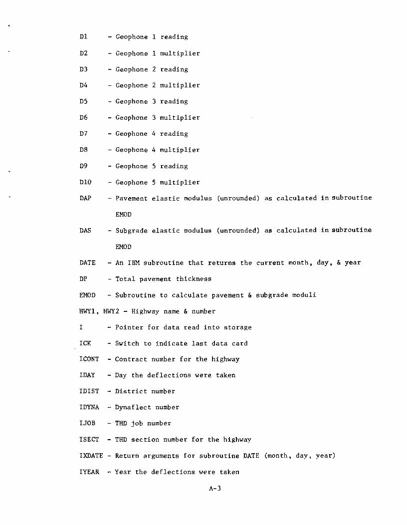
Dl - Geophone 1 reading

D2 Geophone 1 multiplier

D3 - Geophone 2 reading

D4 - Geophone 2 multiplier

D5 - Geophone 3 reading

D6 - Geophone 3 multiplier

D7 - Geophone 4 reading

DB - Geophone 4 multiplier

D9 - Geophone 5 reading

DlO - Geophone 5 multiplier

DAP Pavement elastic modulus (unrounded) as calculated in subroutine

EMOD

DAS - Subgrade elastic modulus (unrounded) as calculated in subroutine

EMOD

DATE - An IBM subroutine that returns the current month, day, & year

DP - Total pavement thickness

EMOD - Subroutine to calculate pavement & sub grade moduli

HWYl, HWY2 - Highway name & number

I - Pointer for data read into storage

ICK - Switch to indicate last data card

ICONT - Contract number for the highway

I DAY - Day the deflections were taken

IDIST - District number

IDYNA - Dynaflect number

IJOB - THD job number

ISECT - THD section number for the highway

IXDATE - Return arguments for subroutine DATE (month, day, year)

IYEAR - Year the deflections were taken

A-3

LAl Description of material in Layer 1

LA2 Description of material in Layer 2

LA1 Description of material in Layer 3

LA4 - Description of material in Layer 4

LAS Description of material in Layer S

LA6 . Description of material in Layer 6

M - Month the deflections were taken

N - Counter for number of error free data cards read

NO - Counter for data cards omitted because of errors

NI - Counter to control printing of 30 lines per page

NCARD - Denotes card type

100 Project identification card

200 Existing pavement description card (layers 1, 2, & 3)

300 Existing pavement description card (layers 4, S, & 6)

400 Data card (geophone readings and multipliers)

PN - Number of test points to be used in the analysis

REM - Any pertinent remarks related to any test point

ROUND - Statement function to round a given value of El or E2 to the

nearest 100 psi

SCI - Surface curvature index, WI - W2, in mils

SEI - Standard deviation of surface curvature index

SE2 - Standard deviation of subgrade moduli

SE3 - Standard deviation of pavement moduli

SRI - Variance of surface curvature index

SR2 - Variance of subgrade moduli

SR3 - Variance of pavement moduli

STA - Station number

Tl - Layer 1 thickness

A-4

T2 - Layer 2 thickness

T3 - Layer 3 thickness

T4 - Layer 4 thickness

T5 - Layer 5 thickness

T6 - Layer 6 thickness

WI - Deflec tion at Geophone number I

W2 - Deflection at Geophone number 2

W3 - Deflection at Geophone number 3

W4 - Deflection at Geophone number 4

W5 - Deflection at Geophone number 5

XLANE - Traffic lane & direction

A-5

Subroutine EMOD Variables

ACC - Test for convergence in iteration for finding E2/E1

AREAl - Result of the integration from x o to x = 3r/h

AREA 2 - Result of the integration from X 3r/h to X = 10r/h

BESJO - Function subroutine to return the Bessel Function Jo(x) for

each x used

DELM1 Increment of m used in interval from m 0 to m 3

DELM2 Increment of m used in interval from m = 3 to m = 10

DELTA - Incremental value for E2/E1 (Sub grade modulus divided by Pavement

modulus) used in iteration process

DELX1 Increment of x in integration from x = 0 to x = 3r/h

DELX2 Increment of x in integration from x = 3r/h to x = 10r/h

E1 - Pavement modu1us(E1)

E2 - Sub grade modulus (E2)

ER Input specifying the accuracy of the iteration in calculating

E2E1

ERROR

FF

FlF2

H

ISW

the ratio E2E1

- Ratio of sub grade modulus to pavement modulus (E2/E1)

- (F1F2 - RATIO), where F1F2 is calculated and RATIO is observed

4TTE) - Function defined as 3P wiri (See Eq. 5)

- Ratio of FF with i = 1 to FF with i = 2

- Pavement thickness, h

- Switch used in iterating to find E2/E1, indicates first time

through the iteration loop

MINUS - Switch used in iterating to find E2/E1, indicates a negative

ERROR

N1 Number of intervals used for integration from x = 0 to x 3r/h

A-6

N2 Number of intervals used for integration from x = 3r/h to x

P - Dynaflect load = 1000#

PARTI - Sum of interior ordinates of first integration

PART 2 - Sum or end ordinates of first integration

PART 3 - Sum of interior ordinates of second integration

PART4 - Sum of end ordinates of second integration

PLUS - Switch used in iterating to find E2/El, indicates a positive

ERROR

10r/h

RH - Radius (distance of geophone from load wheel) divided by pavement

thickness, (r/h)

Rl - Distance from load to Geophone 1

R2 - Distance from load to Geophone 2

RATIO - (WlRl/W2R2)

SAVE - Contains the previous ERROR calculated that is closest to the

convergence criterion in iterating to find E2/El

V - Function subroutine to return the value of V for each E2/El and

XMl values used

- Geophone 1 deflection (mils)

- Geophone 2 deflection (mils)

WI

W2

Xl

X2

XKl

Value of any x in the interval x == o to x == 3r/h

Value of any x in the interval x = 3r/h to x = 10r/h

- Maximum value of 6m in the interval m = o to m = 3 (now set

at 0.01)

XK2 Maximum value of 6m in the interval m 3 to m 10 (now set

at 0.10)

XMl Value of any m in the interval m o to m 3

XM2 Value of any m in the interval m = 3 to m == 10

XN - (El - E2)/(El + E2)

A-7

XNO - Minimum number of values of Jo(x) calculated in the interval

y

from x to x + 3, in the calculation by Simpson's Rule of AREAl

and AREA2. XNO must be an odd number and is now set at XNO 61

- Array to store ordinates to be used in integration from x

to x = lOr/h

A-8

o

Function BESJO Variables

x - Value x in the interval x ::: o to x lOr/h

X3 - X/3, or 3/X if X > 3

X32 - X3 Squared

X33 - X3 Cubed

X34 - X3 to the Fourth Power

X35 - X3 to the Fifth Power

X36 - X3 to the Sixth Power

A-9

Functio~ y Variables

EXPM2M - Exponential, e-2m

EXPM4M - Exponential, e- 4m

XM - Value of any m in the interval m = 0 to m = 10

XN - (El - E2)/(El + E2)

A-lO

Appendix 2

A narrative of the procedure used by ELASTIC MODULUS to calculate

pavement and subgrade elastic moduli is contained on the following

pages.

8-1

The ELASTIC MODULUS program consists of a main pro~ram, two sub­

routines, and two function subroutines. The Main program reads the

input data, performs certain data transformations, and outputs the

results. Subroutine CORE is called by the main pro~ram and is used to

allow the user to select the input format to be used to read a certain

card. The elastic moduli of the pavement and subgrade for each test

point are calculated in subroutine EMOD. The function subroutines BESJO

and V are called by EMOD and are used in the numerical integration used

in calculating the elastic moduli.

The main program reads each input data card into a storage area

and uses subroutine CORE to select the read statement and data format

to read each data card. Subroutine CORE allows a FORTRAN program to

read under format control from a storage area which contains alphabetic

character codes of a card image. Each data card has a code punched in

the first three columns that designates the card type. If the code is

100 the card contains control information about the job, location,

date. and total pavement thickness (see Appendix 4). Card code 200

indicates a card that contains word descriptions and thicknesses of

the first three layers of the pavement (see Appendix 4). The word

descriptions and thicknesses of layers 4, 5, and 6 (if present) are on

cards with code 300 (see Appendix 4). If the card code is 400 or is

blank. the card contains the station number and geophonc readings and

mUltipliers for each observation (see Appendix 4), Cnrd code 100 also

B-2

indicates the beginning of data cards for each job (or set of observations)

and all counters and sums are set to their initial values. The information

on Data Cards 1 and 2 (and Data Card 3, if present) is read and printed

in the heading of the output.

The deflections at each geophone are calculated from the geophone

readings and multipliers on each Data Card 4. SCI = WI - W2 is also

calculated. If either WI or W2 is zero, or if WI is less than W2, an

error message is printed, the observation is not included in the analysis,

and the next card is read. If the quantity WlRl/W2R2 is greater than 1

and the total pavement thickness is less than 9.2" the observation is not

included in the analysis, an error message is printed, and the next card

is read. If WI and W2 are valid observations they are converted to

inches and are passed to Subroutine EMOD along with the total pavement

thickness for the elastic moduli calculation.

The pavement and subgrade moduli returned from EMOD are rounded

to the nearest 100, WI and W2 are converted back to mils, the sums of the

deflections, SCI, pavement modulus, and subgrade modulus are incremented

by the individual observations of each of these variables. The counter

N (the sum of the valid observations) is incremented and a line of out­

put consisting of the station number, WI, W2, W3, W4, W5, SCI, subgrade

modulus, pavement modulus, and remarks is printed. The program will

then skip to a new page before going back to read the next card if 30

lines of output have been printed. If all the data cards have been

read the program calculates and prints averages of all deflections, SCI,

pavement modulus, and the subgrade modulus. The variances and standard

deviations of SCI, pavement modulus and subgrade modulus are calculated

and printed and the program reads Data Card 1 of the next set of ohser­

vations or terminates normally if there is no more data.

B-3

Subroutine EMOD uses the WI, W2, and total pavement thickness from

the main program in the integration process and iteration scheme used to

calculate the pavement modulus, El and the subgrade modulus, E2. All

calculations in EMOD and the function subroutines BESJO and V are done

in double precision to preserve the accuracy of the numerical integra­

tion. The user has the option to change the followin~ variables or

leave them at their present values:

p 1000, ER 0.001, XNO = 61.0, XKl 0.01, XK2 0.10

All switches and counters are initialized, r/h ratios are calculated and

the variable RATIO (used in determining the convergence criterion in

iteration for finding E2/El) is calculated.

DELMI is calculated and tested against the maximum assigned value

for this variable. DELMI is then set to the maximum value or the

calculated value (whichever is the smaller value) and is used in cal­

culating DELXl. DELM2 is calculated and tested in the same manner.

The starting values of DELTA and E2El are selected and XN for the first

iteration is calculated. The iteration loop be~ins with the calculation

of each XN value for each E2El value used.

The number of intervals for each integration, Nl and N2, are cal-

culated. (Note Nl and N2 must be odd integers.) The ordinates for

each x in each integration interval are calculated and stored in the

vector Y. The area of each integration interval is calculated accord­

ing to Simpson's Rule (See Reference 11) and the function FF(l) = AREAl +

AREA2 + 1 is calculated (See Equation 5). FF(2) is calculated as above

except RH(2) is used in calculating DELHI and DELM2.

B-4

ERROR is calculated and tested against the convergence criterion.

If ERROR is < ACC, E1 and E2 are calculated and EMOD returns to the

main program. Otherwise a new value of E2E1 is calculated and the

iteration loop is repeated.

The iteration method consists of trying values of E2E1 until ERROR

is within the convergence criterion. The ERROR for any trial value of

E2E1 that is closest to the convergence criterion is saved so that E2E1

values for subsequent trials can be adjusted to "home in" on the con­

vergence criterion in a minimum number of trials.

For the first trial value of E2E1, if ERROR is not within the con­

vergence criterion, ERROR is stored in SAVE and ISW is set to 1. If

ERROR> 0, PLUS is set to 1 and MINUS is set to O. This indicates ERROR

is positive since PLUS was set to 0 and minus was set to 1 initially.

For each successive pass through the iteration loop the sign of ERROR

determines the segment of code executed to adjust E2E1 for the next

trial until the convergence criterion is met.

When ERROR is positive, E2E1 is adjusted for the next trial in the

following manner. PLUS is set to 1 to indicate ERROR is positive. If

ERROR from the previous trial was positive, E2E1 is decreased for the

next trial and the iteration loop is repeated. If ERROR from the previous

trial was negative, DELTA is decreased by 50%, and the test for SAVE < 0

is made. If SAVE is positive, ERROR is stored in SAVE, E2E] is decreased

for the next trial and the iteration loop is repeated. If SAVE is nega­

tive, the test for I SAVEl > ERROR is made. A true condition indicates

the iteration method is approaching convergence on this trial from the

positive direction so ERROR is stored in SAVE, E2E1 is decreased for the

next trial and the iteration loop is repeated. A false condition indicates

B-S

ERROR is departing from convergence in the positive direction, so E2El is

decreased for the next trial and the iteration loop is repeated.

E2El is adjusted for the next trial in the following manner when

ERROR is negative. MINUS is set to 1 to indicate ERROR is negative.

If ERROR from the previous trial was negative the iteration method is

approaching the convergence criterion from the negative direction, so

E2El is increased for the next trial and the iteration loop is repeated.

If ERROR from the previous trial was positive, DELTA is decreased by

50% and the test for SAVE> 0 is made. A false condition indicates the

previous ERROR was negative also so the test for I SAVEl > I ERROR i is

made. A true condition indicates the iteration method is closer to

convergence on this trial than on the previous trial so ERROR is stored

in SAVE, and E2El is increased for the next trial and the iteration loop

is repeated. A false condition to the above test indicates the previous

ERROR was closer to convergence so increase E2El for the next trial and

repeat the iteration loop. If the test for SAVE> 0 is true. then the

test for I ERROR I > SAVE is made. A false condition indicates the iteration

method is closer to convergence on this trial on the negative side than

the previous trial was on the positive side. so ERROR is stored in SAVE,

E2El is increased for the next trial and the iteration loop is repeated.

For a true condition to the test for \ ERROR \ > SAVE the steps following

the test for \SAVEI > iERRORI are repeated.

The function subroutine BESJO calculates the Bessel Function Jo(x)

using polynomial approximation (See Reference 12) for each value of X

in the integration interval X = 0 to X = lOr/h.

The function subroutine V calculates the value of V (See Equation 2)

for each XN and XMl or XM2 value used.

B-6

..

..

Appendix .1

This appendix contains the ELASTIC MODULI program source deck

set-up .

C-l

Deck Set-Up

The ELASTIC MODULUS program was written in FORTRAN IV, Version G.

The user is advised to change the first read statement in the main program

if the "END=" option of the FORTRAN read is not implemented at his in­

stallation. The user can also substitute any other "Re-read" routine

for Subroutine CORE if this is desired. ELASTIC MODULUS requires

approximately lOOk of core storage and execution time is approximately

7 seconds per test point. The source deck set-up is shown on the

following page.

C-2

•

Source Deck Set-Up for ELASTIC MODULUS Program

,------------I I '

Cards for as Many Additional i AddiU;;-nal Proble;s- - - - - -<. '1~ Problems as Desired ~L---------------------------~ I I

Data Card(s) 4

Control Cards

Function V

Function BESJO

Subroutine EMOD

Main Program

Fortran Control Cards

Subroutine CORE

Cards

Job Card and Hasp Control Cards

C-3

3

2

I I I I I )

_r

Appendix ~

The input format for each data card type used by ELASTIC MODULUS

is included on the following pages. The fields of each card are

delineated and examples of typical data entries for each field are

shown.

D-l

CARD 1

~:- "": c:::t~_ ""I!! o ~_

-I! c:>1:;_ ""I:; ... 1It- ,COMM (I) , I = 1,7) FORMAT 7A4 ",,(I ~II!- Cl'>1I! ... it- Ex. 8 FT. LT. OF CENTERLINE .... It ... j:I- ----------------------------- CI'>!:! ... 1::- Cl'>1:: ... "'- .,.,11: ... I!- -II c:>tiI- ..... ... :a- "';:1 "'1'0- .,.,::; c:>11- on. ... ::1- "'0 c:>;s- ... a ... :a- "'13 . ... :;- -:: =:i- ... a ... :a- enS ... :- ""ill "':11- ell" =tl- ",1;; ola-

i' on" ... /11- ""lit ... :- ""ill =~- .. ,:;I ... :1_ ""!li ... !:t_

_ . ... :-... -. IDYNA 'FORMAT T? H'v =: =111- IDYEAR FORMAT 12 Ex 70 :»'Ii ...... - 'a""" .... - IDAY FORMAT 12 Ex • "7 0'>

... i- .... '

... ,- M FORMAT 12 Ex. -4 "" Clg._ ." ==- "'II =;- DP FORMAT FS.2 Ex. IS.0 '""~ ... ~- ...,

... ~- ----- CIOlI: CI~- ""l!I =\;- <»Ii =:.-... ~- XLANE FORMAT A3 Ex. SBL :: CI;;-

HWYl, HWY2 FORMAT A4, CIOlI;

... ~- A3 Ex. US 290 c'R =R- ------- <»::/ ot=;- <»111 =1iI- ""iii "'IQ- -Ill c:." ...... .... i.i =1:;- IJOB FORMAT 12 Ex. 1 :: I "'111-=~- ISECT FORMAT 12 Ex • 8 ~I ... "'-:~=

enA <»1:1

... ;;- ICONT FORMAT 14 Ex • 114 ... " g::=- enla Q=- ..... c:::J:!!- en 11 c:::tt::- en:: a!!- enl* c::I=:!- <»I!! c::>:£- ... :s c::>!2- <»0

=~- COl, CO2, C03, C04 FORMAT 3A4, A2 Ex. WASHINGTON ..,lJ

c:::t':::-

:~~ a!!- --------------..... - "" .. " c:> .. - <» .. :r ... ~- en,... t::

c:r .. - <» ..

c:o ... - "" .. c:> ... - TDT~T 'FORMAT T? Rv 17 <I> .. ...... - -- -..... - en ..

c:> - - NCARD FORMAT 13 Ex. 100 -----

•

D-2

CARD 2

c:::)~_ en:l c:::)~_ en lie c:::):!:- .n~

<:>1::_ en I:: c:::)=_ en~

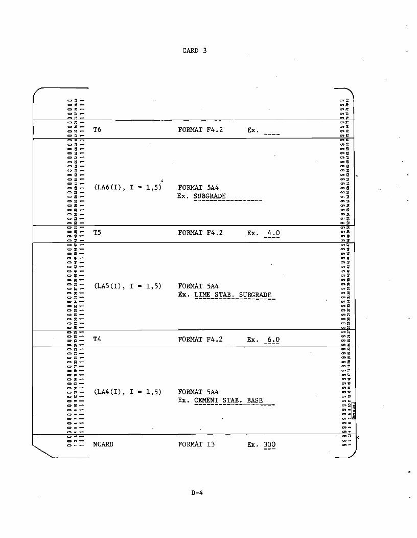
~i!!- enil! c:::)~_ T3 FORMAT F4.2 Ex. 6.0 en;!: <:>~- en~ ----c:>N_ en!:! <:> I: _ c;>I:

<:>~- ",Ii! c:::)=_ en: <:>:a- "':J c:::);_ cn~ c:::)=_ en:l c:::):';:- .... ~ <:>;s- en;l <:>~- (LA3(I) , I 1 ,5~ FORMAT 5A4 ~CI . c:::):i:- = ;:n:ll c:::):'_ en_ QS- Ex. LIME STAB. BASE en: Q::- -------------------- 0::: <:>:- .... " Q:;- ..,.,:.:;

<:>:n- "''' Q:;- a'!::;: <:>~- en~ <:>::1_ 0'::1 Q~- a;~

Q;i- <». <:>ii1- T2 FORMAT F4.2

en:;! Q:- Ex. 8.0 a>: Q:- ---- =3 Q;:- -.:.....,~

Q:- a>~

Q::- en~

<:>#- en# Q~- "'~ ~~- ~:: Q.- ~;

QS- en' Q~- LA2(I), I = 1,5) FORMAT 5A4 enlll <:>~- <nl!! Q~- Ex. IRON ORE BASE en::;

=:01- -------------------- =l!I Q~- enl!; Q~- "'0\ <:>::1_ .,.,::1 c::;- en::' cr:i- en;:; <:>l'I- en:;! Q~- enll: C', - - cnlS <:>1:;- .,,1:; <:>~- T1 FORMAT F4.2 Ex. 1.5 en~

=1Il- en III -----a~_ en;l\ Q~- cr.,. Q:::- en:::: <:> ... - en ... <:>2- en~ c!!_ en!!! <:>~- en~ Qe _ en I: Q~- en!!! Q~- a>\!! <:>:t- (LAl(I) , I = 1,5) FORMAT 5A4 en:t <:>11- en II Q~- Ex. ASPHALTIC CONCRETE

en", Q::-

:~~ Q~- ---------------------<:> - - en G ~

<:> .. - en .. !: <:> - - en - -<:> .. - en .. <:> .. - "'--c.-- en .-<:> .. - Q> ..

<:> .. - NCARD FORMAT 13 200 en ..

<:> - - Ex. en ----

•

D-3

o I .p-

00

01

00

00

00

00

00

00

00

00

00

0 O~

O U

0 01

0 0

0 0

0 0

00

00

00

00

00

00

0 D

ID D

O DI

D 0

0 0

0 0

00

00

00

00

00

00

00

10

0 0

O~

DO

DD

lZ~456 l"~"UUM~~naWH~nn4nHUHH~~u~~n~n~n~~QQ~U"U"Q~~U~MHH~HH"~U~H~"UNUWnnnMn

nn

nu

1

11

11

11

11

11

11

11

11

11

11

11

11

11

11

11

11

11

11

11

11

11

11

11

11

11

11

11

11

11

11

11

11

11

11

11

11

11

11

11

1

z (") ~ t'%j

o ~ H

W

t>:l ><

IW

10

1

0

,-...

t"

' ~

,-...

H

'"'"

H II I-'

U1 '"'"

t>:l

t'%

j ><

0

~~

t>:lt

-'3

~U1

Z>

t-

'3.p

-

UJ ~ ~ . ~

It>:l

I I I

t-'3

.p- d ~ t'%j

.p-

N

t>:l ><

I 10

\ I·

1

0

,-...

t"

' >

U1

,-...

H

'"'"

H II I-'

U1 '"'"

tfd

,~ ~

IH

t-'3

l~ U

1 I

>

I UJ

.p-

1t-'3

I>

I~

I •

I IUJ

Ie::

I~

1G1 !~

It>:l

I

t-'3

U1

t'%j o ~ t-'3

t'%j

.p-

N

t>:l ><

I I.p

­I·

1

0

,-...

f; 0\

,-...

H

'"'"

H 1\ I-'

U1

'-" ;

,.,

t>:l

t'%

j ><

0 ~~

~

G1

U1

~~

t>:l

t-'3

0\

t'%j o ~ t'%j

.p-

N

t>:l ><

99

91

99

99

9 9

99

99

S 9

99

99

99

99

19

9 S

!l19

99

99

99

9 9

9 S

9 9

!l 9

9 9

9 9

~19

9 9 91~

C! 9

~ 9

9 9

9 9

99

99

99

99

99

91

99

99

19

9 S

9 9

lZJ451,a'~"UUMGWnaWH~nnNnHuua~~uu~~HnnU~~QQ~~~U"Q~M~~M~~~WH"~~~H~n~uu~nnnMnnnnnu

~

'"

§ W

CARD 4

/ c::::)5:- "': c::::)~_ ao:!! c::::):e- on:!! <:>1':_ "'I: c::::):!_ ICK FORMAT 12 Ex. 99 O>~

<:>I(!- Q>~

Q;t- Q>;!: <:>r::!- Q>::! Q~- Q>~

<:>"'- ""'" Q2- C1~ Q::- Q>S Q~- Q>: QC;-

(REM(I), ~~

Q::- I = 1,4) FORMAT 4A4 Ex. WEST BOUND LANE <nlJ: Q~- ---------------- en:!: <:>;J- Q>;J QQ- 0:":1:3 Q:t:- =:;: QC;- <1>;;;

Qfi;- Q>~ Q:t- ",,'"

<:>~- .,,~

Q:;;- .,:r,~

Q::- cn~ Q:::;- ~:a Q:;- Q'J~ <:>:;!- O~~

Q:;;- o;~

Q:;;- 0'> ..

Q~-

D10 FORMAT F3.2 Ex. 010 =:il

Q~- ~~ Q:;- --- "'~ Q:;;:- D9 FORMAT F2.1 Ex. 37

-:n :; Q:- "':= Q~- Q>" <:>~- D8 FORMAT F3.2 Ex. 010 Q>~

Q~- :n~ <:>.- D7 FORMAT F2.1 Ex. 45 :n:;! a;_ =":i Q~- C). Q=- D6 FORMAT F3.2 Ex. 010 a>i!; Q~- - ml": Q~-

D5 FORMAT F2.1 Ex 6Q 0>::;

a~_ =~ <:>~- -- Q>;" <:>;1;_ D4 FORMAT F3.2 Ex. 030 .,,;7; <:>::1_ -- <. .... ::1 =ft- D3 FORMAT F2.1 Ex. 30 O>~

a;;;_ "'M <:>~- Q>~

<:>1::- D2 FORMAT F3.2 Ex. 030 en I: CI ~_

C")~

0:;;-D1 FORMAT F2.1 42

.,,1:;

Q~- Ex. a>~ 01';- - Q> ...

Qit- Q>;:; Q~- ~::

<:> ... - Q>:::l <:> N- Q>N Q2- "':;: Q~- STA FORMAT A7 Ex. 248+00 Q>!!! Q=- Q>!!! -------Qt::- ",t:: o~- O>!!! Q~- IYEAR FORMAT 12 Ex. 70

Q>!!! <:>:!- "':! 0:2- I DAY FORMAT 12 Ex. -7 Q>12 Q:=!- Q>!::I ~::- M l"UKMAT 12 Ex. -~ :;rc Q~-

<:>"'- ISECT FORMAT 12 Ex. 8 Q> :I~ <:> "'- '" '" . <:> ~ .... en ... L: <:> ~ .... ICONT FORMAT 14 Ex. ll8 en w

<:> ~- <1> .. ----<:> ...... <n .-<:>" .... Q) .. t <:> N .... NCARD FORMAT 13 Ex. 400 Q> N

<:> - .... Q> ----

D-5

Appendix 1

This appendix contains the flowchart of the procedure used in

ELASTIC MODULUS to calculate a pavement or subgrade modulus.

E-1

READ

START

STOP

?

NO

NCARD & remainder of card into the A array

CALL CORE

NO

READ Card 1 - Control information, Highway, County, District, Date, & Comments

CALL DATE

WRITE Control information & date at top of page

Initialize all Counters, Sums & Variances to Zero

READ

NO

Card 2 - Layer 1, 2 & 3 Descriptions & Layer 1, 2 & 3 Thicknesses

E-2

WRITE

READ

& 3 Descriptions 2 & 3 Thicknesses

NO

Card 3 - Layer 4, 5 & 6 Descriptions & Layer 4, 5 & 6 Thicknesses

WRITE Layer 4, 5 & 6 Descriptions & Layer 4, 5 & 6 Thicknesses

READ

Increment pointer I

Card 4 - Control information, Station, Geophone readings &

~ __ ~M~u=lti liers

WRITE

GT 0 ?

YES

YES

Output column headings

Calculate WI, W2. W3, W4, W5 & SCI

YES

E-3

YES

ADD to Sums

Convert WI & W2 to inches

WRITE

Increment NO

Call EMOD to calculate pavement modulus & subgrade modulus No Solution

Round pavement modulus to nearest 100

Add to sums

WRITE

AAS2 = AAS2 + AS2 AAP2 AAP2 + AP2

Increment N

Station, WI, W2, W3, W4, W5, SCI, sub­grade modulus, pavement modulus, remarks.

NO

WRITE Output column headings on next page

E-4

Nl o

YES

},N = N

Calculate Avg. deflections, Avg. SCI, Avg. pavement modulus, Avg. sub rade modulus

Calculate variance of SCI, Avg. pavement moduli & subgrade moduli

WRITE Avg. deflections, Avg. SCI, Avg. Pave­ment modulus, Avg. subgrade modulus

YES

Calculate standard deviation of SCI, Pavement moduli & sub rade moduli

WRITE Standard deviation of SCI, Pavement moduli, subgrade moduli

WRITE No. of Test Points used in Analysis

E-5

J --...... 1---""

I

I I I I

,..- -

SUBROUTINE EMOD

ENTRY

Set all switches, initialize all sums & constants

Calculate RH(l) & RH(2) , RATIO, ACC

Do from 1 to 2

Calculate DELMI = (l/RH) * (3/XNO - 1)

YES

NO

Calculate DELXl = DELMI * RH

Calculate DELM2 = (l/RH) * (3/XNO - 1)

YES

NO E-6

, I

I I I I I

I I

I

I

I I I

I

I I f I

\

.....

I Calculate DELX2 .. DELM2 * RH

"'---- - -----"

,-- -

DELTA .. 0.5 E2El ... 001

Calculate XN, XN .. (El - E2)/(El + E2)

Do from 1 to 2

Calculate Nl, No. of intervals for in­tegration by Simpson's rule from X .. 0 to X .. 3mr/h

Calculate N2, No. of intervals for in­tegration by Simpson's rule from X = 3mr/h to X .. 10mr/h

Set XMl = 0.0

Xl .. 0.0

,

E -7

1

,..-

\ -

I' ,

I

I I I \ --

t Do from 1 to Nl

Calculate the ordinates for integration for interval X = 0 to X = 3mr/h y = [V(XN, XM) - 1] * BESJO (Xl)

Increment XMl & Xl, XMl = XMl + DELM1, Xl = Xl + DELXl

- - - I

I XM2 = XMl , X2 = Xl

l Do from 1 to N2

I Calculate the ordinates for integration for interval X = 3mr/h to X = tOmr/h,

• y = [V(XN, XM2) - 1] * BESJO (X2)

Increment XM2 & X2, XM2 :: XM2 + DELM2, X2 = X2 + DELX2

--- CONTINUE I E-8 ,

/'-

I I

I I \ -

-

f PARTl = 0.0 PART2 = 0.0

Calculate N4, No. of interior ordinates under curve from X = 0 to X = 3mr/h, N4 = N1 - 3

Do from LL = 2 to N4, incrementing LL by 2

Sum interior ordinates, PARTl = PART 1 + 2 '* Y (LL) + Y(LL + 1)

- - CONTINUE

Sum the end ordinates

PART2 = Y(l) + 4 * Y(N1 - 1) + Y(N1)

Calculate area of integration from X = 0 to X = 3mr/h AREAl = «2 * DELX1)/3) * PART1 +

(DELX1/3) * PART2

,r E-9

,

Calculate position of first interior ordinate for integration from X = 3mr/h to X = lOmr/h, NS = Nl + 2

Calculate position of last interior ordinate for integration from X = 3mr/h to X = lOmr/h, N6 = N2 - 3 + Nl

,,-- - Do from LM = NS to N6, incrementin~ LM BY 2

Sum interior ordinates for interval X = 3mr/h to X = lOmr/h PART3 = PART3 + 2 * Y(LM) +

Y(LM + 1)

CONTINUE

Sum end ordinates of interval from X = 3mr/h to X = lOmr/h PART4 = Y(Nl + 1) + 4 * Y(Nl + N2

- 1) + Y(Nl + N2)

Calculate area of integration from X = 3mr/h to X = lOmr/h, AREA2 = «2 * DELX2)/3) * PART3

+ (DELX2/3) * PART4

III

E-10

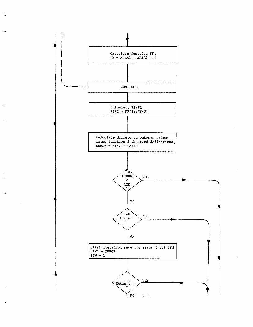
I I I I I \ - --

Calculate function FF, FF = AREAl + AREA2 + I

CONTINUE

Calculate FI/F2, FIF2 = FF(I)/FF(2)

Calculate difference between calcu­lated function & observed deflections, ERROR = FIF2 - RATIO

YES <

YES

NO

First iteration save the error & set ISW SAVE • ERROR ISW I

YES

E-ll

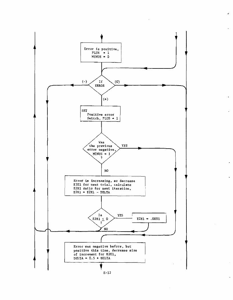
Error is positive, PLUS 1 MINUS = 0

(-)

SET

(0)

(+)

Positive error Switch, PLUS'" 1

Was previous YES

error negative, >-------~~--------------­MINUS-1

?

NO

Error is increasing. so decrease E2E1 for next trial, calculate E2E1 ratio for next iteration. E2E1 .. E2E1 - DELTA

Error was negative before, but positive this time, decrease size of increment for E2E1. DELTA" 0.5 * DELTA

E-12

Is SAVE < 0

?

YES

Calculate E2El ratio for next iteration, E2El ~ E2El - DELTA SAVE ERROR

YES

?

NO

Error is increasing in positive direction, decrease E2El for next iteration, E2El = E2El - DELTA

SET Negative error switch, MINUS 1

E-13

NO

Error is on Negative side. Increase E2El for next iteration. E2El = E2El + DELTA

NO

Delta too Large Iteration Process will be divergent, Decreases size of Delta, DELTA = 0.5 * DELTA

Error is on Negative side But the iteration process is Divergent, Decrease E2El for Next iteration E2El = E2El - DELTA

Error was positive before, but is negative this time, decrease size of Delta, DELTA = 0.5 * DELTA

E-l4

Calculate E2EI ratio for next iteration, E2EI • E2EI + DELTA

YES

NO

Calculate, E2EI ratio for next iteration E2EI == E2EI + DELTA SAVE == ERROR

Calculate EI & E2, EI == (3 * P * FF(I)/(4 * PI * WI * RI) E2 == E2EI * EI

E-15

FUNCTION BESJO

ENTRY

Calculate X3, X3 = X/3

YES

Calculate Constants, X32 = X3 * X3 X33 = X32 * X3 X34 '" X32 * X32 X35 = X32 * X33 X36 ;: X33 * X33

Is Ixi 2. 3

?

NO

YES

Calculate BESJO(X) for X > 3

RETURN

END

E-16

X3 3/x "

Calculate BESJO(X) for

X2. 3

FUNCTION V

ENTRY

Set V :: 1

YES

NO

Calculate Function V

RETURN

END

E-17

Appendix ~

On the following pages is a listing of ELASTIC MODULUS with the

output from a sample problem. The input data cards for the sample

problem are listed after the program output.

F-l

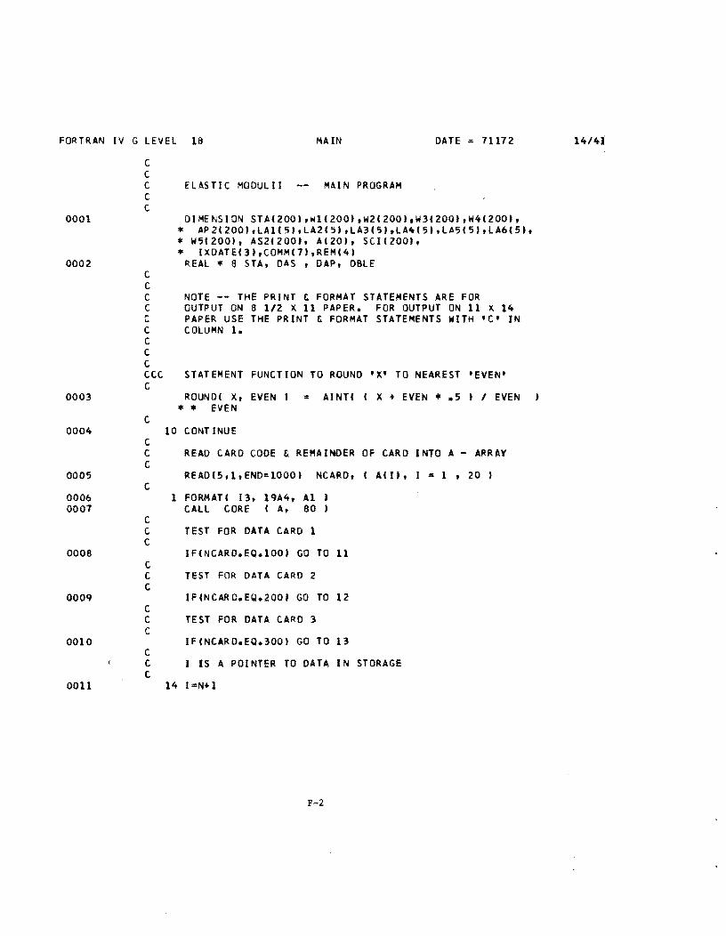
FORTRAN IV G LEVEL 18 MAIN DATE: 71172

C C C C C

ELASTIC MODULII MAIN PROGRAM

0001 DIMENSION STAC200t,w1C200t.W2C200t.W3C200t,W4C200t, * AP2(200),lAICSt,lA2C5t,lA3ISttlA~ISt,lASIS),lA6C5t, * WSCZOO), AS2C2001, A120t, SCIC200', • IXDATEC3J,COMM(7),REMC4)

0002 REAL • 8 STA, DAS , OAP, DBlE

0003

C C C NOTE -- THE PRINT & FORMAT STATEMENTS ARE FOR C OUTPUT ON a l/Z x 11 PAPER. FOR OUTPUT ON 11 X 14 C PAPER USE THE PRINT & FORMAT STATEMENTS WITH 'C' IN C COLUMN 1. C C C CCC STATEMENT FUNCTION TO ROUND 'X' TO NEAREST 'EVEN' C

C

ROUNDI X, EVEN I ~ AINTC C X + EVEN •• 5 J / EVEN •• EVEN

0004 10 CONTINUE C C READ CARD CODE & REMAINDER OF CARD INTO A - ARRAY C

OOOS READC5,1,END=1000J NCARD, C ACII, I = 1 , 20 ) C

0006 1 FORMAT( 13, 19A4, A1 0007 CALL CORE (A, 80

C C TEST FOR DATA CARD 1 C

0008 IFCNCARD.EQ.100J GO TO 11 C C TEST FOR DATA CARD 2 C

0009 IFCNCARD.EQ.2001 GO TO 12 C C TEST FOR DATA CARD 3 C

0010 IFCNCARD.EQ.300) GO TO 13 C C I IS A POINTER TO DATA IN STORAGE C

0011 14 l=N+l

F-2

14/41

FORTRAN IV G LEVEL 18 MAIN DATE = 11112

0012

0013

0014 0015

0016

0017

0018 0019 0020 0021 0022 0023

0024 0025

0026 0027 0028 0029 0030 0031 0032 0033

0034

C C C

C

C

C C C

c c

C

RfAO DATA CARD 4

REAOI5,61 ICONT,ISECT,M,IOAY,IYEAR,STAIII,01,02,03, * 04, 05, 06, 07, 08, *09,010,IREMIJI,J=1,41,ICK

6 FORMAT I

IFI N.GT. 0 I GO TO 555 IFINO.GT.OI GO TO 555

PRINT OUTPUT COLUMN HEADINGS

PRINT 61 61 FORMATI/,lX,'STATION Wl W2 W3 W4 "

= '1015 SCI ** ES ** ** EP ** REMARKS' I I 61 FORMATII 7X,'STATION loll W2 W3 W4 W5', .' SCI ** ES ** ** EP ** REMARKS'/I

C CALCUL~Te DEFLECTIONS & SCI 1 DEfLECTIONS IN MILS I C

C C C

C

C C

C C

555 1011111=01*02 W2III=03*04 W31Il z 05*06 W41I 1=07*08 W5II,=09*010 SCIIII=Wlll'-W2II1

TEST FOR loll OR 1012 = 0, AND loll LESS THAN 1012

IF IW1III.EQ.0.OR.W2III.EQ.01 GO TO 64 IFIW1III.LT.W2III1 GO TO 66

AWl =AWI +1011 III AW2 =AW2 +1012 III AW3 =AW3 +10131 I I AW4 =AW4 +1014111 AW5 =AW5 +10151 I I ASCI=ASCI+SCl( I I AS21 I I 0.0 AP 2( I J = 0.0

IFI ( W1<IJ * 10.0 I I I W21I1 * SQRTI 244.0 I I = .GT. 1.0 .AND. DP .LE. q.l J GO TO 60

F-3

14/41

FO~TRAN IY G lEYEl 18 MAIN DATE = 11172

0035 0036

0037

0038 0039

0040 0041

0042 0043

0044 0045

0046

C CONVERT ~1 & W2 TO INCHES C

C C C C C

C C C

C C C C C C

C

'11(11 = 'Ill II I 1000. W21lJ = '1211' I 1000.

PASS '11, w2, t TOTAL PAVEMENT THICKNESS TO EMOD, EMOD RETURNS UNROUNDED VALUES OF PAVEMENT t SUBGRADE MODUll1 AS DAP & DAS

CAll EMOD I D8lEIW1Ii", DBlEIW2'I", DBlE'DP',DAP, DAS'

CONYERT wi t w2 TO MilS

win' '1111' * 1000. '12(1' = W2CI' * 1000.

ROUND PAVEMENT & SUBGRADE MODUllI TO NEAREST 100

DAS = ROUNDC DAS, 100. 1 DAP '" ROUNDC DAP, 100. 1

C PUT PAVEMENT & SUBGRADE MODUlII IN STORAGE C

c C C C

C C C

C

AS2'11 = DAS AP2(11 = DAP

ADO TO THE SUMS OF THE DEFLECTIONS, SCI, PAVEMENT, AND SUBGRADE MODULII

AAS2:AAS2.AS2' I 1 AAP2=AAP2·AP2111

ADD TO N, THE NUMBER OF VALID TEST POINTS

C PRINT A lINE OF OUTPUT C C PRINT 63,STACII,W1CIJ,W2CII,W3(II,W4CII,W5CII,SCIIII, C = AS2III, AP211', ( REMCJI,J=l,4 I C 63 FORMAT(lX, A7, 3X, 5(F5.3,2X I, F5.3,2F11.0,5X,4A4 I

0047 PRINT 63,STA(II,W1(II,W2CII,W3(I),W4(1),W5(II,SCI(II, * AS2UI, AP2UIt (REM(JI,J=l,2.

0048 63 FORMATI 7X,A7,lX,6(F6.3I, 2F10.0,2X, 2A4 0049 Nl = Nl • 1

F-4

14/4)

FORTRAN IV G LEVEL 18 MA IN DUE 11172 lit I 4]

0050 IF(1II1.LT.301 GO TO 88 C C SKIP TO NEXT PAGE & PRINT OUTPUT COLUMN HEADINGS IF C THIR TV LINES HAVE BEEN PRINTED C

0051 84 CONTINUE 0052 PRINT 51

C PRINT 56 C PRINT 57,IDIST,C01,C02,C03,C04,ICONT,ISECT,IJOB,HWY1, C • HWY2, XLANE, M, IDAY, IYEAR, IDYNA

0053 PRINT 56, IDIST, COl, C02, C03, C04 0054 56 FORMAT( T35,'DIST. COUNTY'I T36, I2,9X, 3A4,A2 II 0055 PRINT 57, ICONT, ISECT,IJOB,HWY1,HWY2,M,IDAy,IYEAR,IDYNA 0056 57 FORMAT( T19, 'CONT. SECT. JOB HIGHWAY DATE',

DYNAFLECT' I T19,14,2I7,4X,A4,A3,14,2('-',I21,19 II 0057 PRINT 61 0058 Nl K 0 0059 88 CONTINUE

C C CHECK FOR LAST DATA CARD 4 C

0060 IF (ICK.EQ.OI GO TO 10 0061 GO TO 80

C C READ DATA CARD 1 C

0062 11 READ(5,21 IDIST,C01,C02,C03,C04,ICONT,ISECT,IJOB,HWY1, • HWY2, XLANE, DP,M,IDAY,IYEAR,IDYNA,(COMMCII,I=1,71

0063 2 FORMAT( 12,3A4,A2,I4,2I2,A4,A3,A3,F5.2,4I2,7A41 C C PRINT HEADING C

0064 PRINT 51 0065 51 FORMAT( '1' I

C 0066 PRINT 52

C 52 FORMATC33X,'TEXAS HIGHWAY DEPARTMENT',/I 0067 52 FORMAT(35X, 'TEXAS HIGHWAY DEPARTMENT' II

C 0068 PRINT 53,IDIST

C 53 fORMATC31X,'DISTRICT ',12,' - DESIGN SECTION',/I 0069 53 FORMAT(33X,'DISTRICT ',12,' - DESIGN SECTION' II

C 0070 PRINT 54

C 54 FORMATC16X,'DYNAFLECT DEFLECTIONS AND CALCULATED " C = 'ELASTIC MODULII' I I

0071 54 FORMATC21X,'DYNAFlECT DEFLECTIONS AND CALCULATED " • 'ELASTIC MODULII' I I

F-5

FORTRAN IV G LEVEL 18 MAIN DATE 71172

0072

0073

0074

0075

0076

0077 0078

0079 0080 0081 0082 0083 0084 0085 0086 0087 0088 0089 0090 0091 0092

0093

0094

0095

C C C

C

GET CURRENT DATE

CALL DATE C IXDATECll, IXDATEC21, IXDATEC31

PRINT 55,IXDATE C 55 FoRMATC30X,'THIS PROGRAM WAS RUN - ',2A3,A2 I

55 FoRMATC32X,'THIS PROGRAM wAS RUN - " 2A3,A2 I C C PRINT 56 C 56 FORMAT( lX,'DIST. COUNTY CaNT. C *' JOB HIGHWAY DATE DYNAFLECT'I

PRINT 56, IOIST, COl, C02, C03, C04 C C PRINT CONTROL INFORMATION FROM DATA CARD 1 C

SECT.',

C PRINT 57,IDIST,C01,C02,C03,C04,ICoNT,ISECT,IJOB,HWY1, C * HWY2, XLANE, M, IOAY, IYEAR, IDYNA C 57 FORMATC 2X,I2,5X,3A4,A2,3X,I4,4X,I2,5X,I2,2X,A4,A3, C * A3, 2X, 12, '-', 12, '-', 12, 6X, 12 I I

C

C C C

C

C C

PRINT 57, ICoNT, ISECT,IJoB,HWYl,HWY2,M,IDAY,IYEAR,IDYNA

PRINT 58'(CoMMC I) ,1=1,71 ,DP 58 FoRMATC10X,7A4.2X,·PAV. THICK. = ',F5.2,' INCHES' ,II

INITIALIZE ALL SUMS & COUNTERS

N=O N1 = 0 NO = 0 AW1= o. AW2=0. AW3=0. AW4=0. AW5=0. ASCI=O. AAS2=0. AAP2=0. SRI: O. SR2= O. SR3= O.

GO TO 10 READ & PRINT INFORMATION ON DATA CARD 2

12 READC5,3) CLA1CII,I=1,51.Tl,CLA2CII,I=1,51,T2, * CLA3CIltI=1,5I, T3

3 FORMATC 5A4,F4.2,5A4.F4.2,5A4,F4.21

F-6

14/4J

FORTRAN IV G LEVEL 18 MAIN DATE '= 71172

0096 0097 0098 0099

0100

0101 010Z 0103 0104

C C C

C C C

C C

C

PRINT 59,CLAlCII,I=l,5I,Tl,CLAZCII,I=l,5I,TZ, • CLA3CII.I=l,5I, T3

59 FORMATC 1X,5A4,lX,F5.Z,ZX,5A4,lX,F5.Z,2X,5A4,lX,F5.21 PRINT 59,CLA1CII,I=l,5I,T1,CLAZCII,l z 1,5I,T2 PRINT 59, C LA3CII, 1=1,51, T3

59 FORMATC16X, 5A4, lX, F5.2, 5X, 5A4, lX, F5.211 GO TO 10

READ & PRINT INFORMATION ON DATA CARD 3, IF PRESENT

13 READC5,31 CLA4CII,I=1,5I,T4,CLA5CII,I=1,5t,T5, • CLA6ClI,I::1,51, T6

PRINT 59,CLA4CII,I=1,51,T4,CLA5CII,I=1,51,T5, • CLA6CII,I=1,51, T6

PRINT 59,CLA4CII,I=1,51,T4,CLA5CII,I-1,51,T5 PRINT 59, C LA6fll, 1=1,51, T6 GO TO 10

66 NO = NO+1

C PRINT NEGATIVE SCI MESSAGE C

0105 PRINT 82,STACII,W1CII,W2CII,CREMCJI,J=1,41 0106 82 FORMATC1X,A7,3X,F5.3,2X,F5.3,2X,'NEGATIVE SCI OTHER I,

0107 0108 0109 0110

• 'CALCULAT IONS OMITTED', 4X, 4A41 C

C

N1=N1+1 IF C N1 GO TO

64 NO :: NO

.LT. 84 + 1

30 I

C PRINT ERROR MESSAGE C

GO TO 88

0111 PRINT 81,STACII,CREMCJt,J=1,41 011Z 81 FORMATC 1X,A7,3X,'DATA ERROR ASSUMED A ZERO VALUE RE',

0113 0114 0115

0116 0117 0118 0119

0120

C

C C

• 'AD FOR W1 OR W2', 5X, 4A4 t

N1 = N1+ 1 IF C N1 .LT. 30 I GO TO 88 GO TO 84

60 CONT INUE N .:: N + 1 NO :: NO + 1 PRINT 85, STACII, W1CII, WZCII, W3C11, W4CIt,

W5ClI, SCICli 85 FORMATC 7X, A7, lX, 6F6.3, 2X,

'NO UNIQUE SOLUTION' I

F-7

14/4]

FORTRAN IV G LEVEL 18 MA IN DATE 71172

0121 0122 0123

0124 012'5 0126 0127 0128 0129 0130 0131 0132 0133 0134

0135 0136 0137 0138 0139 0140 0141

0142

0143

0144 0145 0146

0147 0148

C C C

N 1 Nl + 1 IFI Nl .LT. 30 GO TO 84

GC TO 88

C ALL CARDS READ FOR AN ANALYSIS, CALCULATE AVERAGE C DEFLECTIONS, AVERAGE SCI, AVERAG~ PAVEMENT MODULUS, C AND AVERAGE SUBGRAOE MODULUS C

C C C C

C C C

C

C C C C

C C

80 PN=N Nl N NO IFI Nl .LE. 0 AWIV= Awl/PN AW2V= AW2IPN AIo/3V= Aw3/PN Aw4V= AW4/PN AIo/5V= AIo/5/PN ASCI V=ASC IIPN AAS2 V=AAS2INl AAP2V=AAP2INl

Nl 1

CALCULATE VARIANCE OF SCI, SUBGRADE MODULUS & PAVE­MENT MODULUS

DO 62 I=l,N IFIWlII I.EQ.0.OR.w2CI I.EQ.OI GO TO 62 SR1 = SR1 + «ASCIV- SCI(I))**2) IF( AS2(I) .EQ. 0.0) GO TO 62 SR2= SQ2+( IAAS2V-AS21 I 11**21 SP3= SR3+IIAAP2V- AP21[1)**21

62 CONTINUE

PRINT AVERAGES

PRINT 65,AwlV,AIo/2V,AIo/3V,Aw4V,Aw5V,ASCIV,AAS2V,AAP2V 65 FORMAT(/lX,'AVERAGES', 612X, F5.3 I, 2Fll.0 1 65 FORMATI/ 7X, 'AVERAGES', 6IF6.31, 2FIO.0 I

CALCULATE STANDARD DEVIATION OF SCI, SUBGRADE MODULUS, AND PAVEMENT MODULUS

IFI PN .EQ. 1. 1 GO TO 90 SEl SQRT(SP1/IPN-l)) IF( N1 .LE. 1) GO TO 90 SE2 = SQRT(SR2!(N1-1)) SE3 = SQRT(SR3!(N1-1))

PRINT STANDARD DEVIATIONS

F-8

14/41

FORTRAN IV G LEVEL 18 MAIN OATE 11112

C 0148 PRINT 11,SE1,SE2,SE3

C 11 FORMATC 1X,'STANOARO DEVIATION',21X,F5.3, 2F11.0 0149 11 FORMATC 1X,'STANDARD DEVIATION', 20X,F6.3,2F10.0.

0150 0151 0152

0153

0154

0155

0156

0151

C

C C

C

90 CONTINUE IFC N .EQ. 1. N1 PR INT 99,N, N1, N1

99 FORMATC1X,'NUMBER OF 114, 19, 110 •

99 FORMATC 1X,'NUMBER 114, 19, 110 •

PRINT 91

= 1

POINTS IN AVERAGE = "

OF POINTS IN AVERAGE = "

C 91 FORMATC 1,5X,'W1 91 FORMATe/10X,'W1

DEFLECTION AT GEOPHONE 1'. DEFLECTION AT GEOPHONE 1'.

C PRINT 92

C 92 FORMATe 5X,'W2 92 FORMATC 10X,'W2

C

DEFLECTION AT GEOPHONE 2'. DEFLECTION AT GEOPHONE 2'.

0158 PRINT 93 C 93 FORMATC 5X,'W3 DEFLECTION AT GEOPHONE 3 ..

0159 93 FORMATC 10X,'W3 DEFLECTION AT GEOPHONE 3'. C

0160 PRINT 94 C 94 FORMATe 5X,'W4 DEFLECTION AT GEOPHONE 4'.

0161 94 FORMATe 10X,'W4 DEFLECTION AT GEOPHONE 4'. C

0162 PRINT 95 C 95 FORMATe 5X,'W5 DEFLECTION AT GEOPHONE 5"

0163 95 FORMATe 10X,'W5 DEFLECTION AT GEOPHONE 5'. C

0164 PRINT 96 C 96 FORMATe 5X,'SCI SURFACE CURVATURE INDEX C loll MIN', C = 'US 1012 ...

0165 96 FORMATC 10X,'SCI SURFACE CURVATURE INDEX e loll MIN', • 'US 1012.' •

C 0166 PRINT 91

C 91 FORMATe 5X,'ES ELASTIC MODULUS OF THE SUBGRADE FRO', C = 'M loll AND 1012'

0161 91 FORMATe 10X,'ES ELASTIC MODULUS OF THE SUBGRADE FRO', • 'M loll AND 1012' •

C 0168 PRINT 98

C 98 FORMATC 5X,'EP ELASTIC MODULUS OF THE PAVEMENT FROM', C =' loll AND 1012'

F-9

14/41

FORTRAN IV G LEVEL lB

0169

0170 0171 0172

C C

98 FORMAT! 10X,'EP * 'M Wl AND W2' I

GO TO 10 1000 CONT INUE

END

•

MAIN DATE = 71172 14/41

ELASTIC ~ODULUS OF THE PAVE~ENT FRO',

F-IO

FORTRAN IV G LEVEL 18 EMOO DATE = 11112

0001

0002 0003

0004 0005

0006

0001 0008 0009 0010 0011 0012

0013 0014 0015 0016

0011

0018

0019

0020

0021

c C

C

C C C

C

SUBROUTINE EMOO I loll, \012, H, Elf E2

IMPLICIT REAL * 8 I A-H, O-Z I DIMENSION RHI 21, FFI 21, Y(4000), OELM1I21,

OELM2121, OELXlC21, OELX2121

DATA P / 1000.000 / , ER / .00100/ DATA XNO / 61.000 /, XK1 / 0.0100 /, XK2 / 0.1000 /

p, XNO, XK1, XK2, R1 & R2 CAN 8E CHANGED IF DESIRED

INTEGER PLUS

C INITIALIZE SWITCHES & SAVE C

C

R1 = 10.000 R2 ;; OSQRTI 244.000 MINUS :: 1 PLUS = 0 ISW = 0 SAVE = 0.000

C CALCULATE R/H, RATIO, & ACC I ACC IS THE CONVERGENCE C CRITERION I C

C C

C C C

C

C C C

C C C

*

RHIU R1 / H RHI21 R2 / H RATIO : I loll * Rl I / I W2 * R2 I ACC = ER * RATIO

DO 2 KL = 1, 2

CALCULATE AND TEST OELM1

DELMlIKLI ;; I 1. 000 / R HI K L , I * C 3.000 I C XNO - 1.000 I ,

IFC XK1 .LE. OELM1(KLI DELMlIKLI .. CALCULATE DEL Xl

DELX lC KL, OELM1CKLI * RHCKLI

CALCULATE AND TEST OELM2

OELM2IKL, = I 1.000 / RHCKLI, • C 3.000 I

F-ll

XKl

14/4J

FORTRAN IV G LEVEL 18 EMOO DATE z 71172

0022

0023 0024

0025 0026

0027 0028

0029

0030 0031

0032 0033

0034 0035 0036 0037 0038 0039 0040

* XNO - 1.000 I I C

IFI XK2 .LE. OELM21KLI OELM2(KLI z XK2 C C CALCULATE OELX2 C

C C

OELX21KLI s OELM21KLI * RH(KLI 2 CONTINUE

C GET INITIAL VALUE OF E2/El AND DELTA C

C C

DELTA = 0.500 E2El = 0.00100

C START ITERATION LOOP FOR EACH E2/El VALUE USED C

4 CONTINUE XN I 1.000 - E2El I I I 1.000 + E2El

C C THE FUNCTIONS FFlll AND FFI21 ISEE EQN. 51 ARE C CALCULATED IN THE FOLLOWING 00 LOOP. C

C C C C

C

C C C C

C 28

DO 29 KK = 1 2

CALCULATE NO. OF INTERVALS FOR SIMPSON'S RULE FOR EACH INTEGRATION. Nl & N2 MUST BE ODD INTEGERS.

Nl = (3.000 * RH(KKI I I OELXllKKI + 1.000 IF(INl I 21. 2 .EQ. Nll Nl ~ Nl + 1

N2 = '7.000 * RHIKKI I I OELX2(KKI + 1.000 IF(IN2 121 * 2 .EQ. N21 N2 = N2 + 1

CALCULATE ORDINATES FOR SIMPSON'S RULE FOR FIRST INTEGRATION

XMl = 0.000 Xl z 0.000

DO 28 JJ z 1, N1 Y(JJI ( VI XN, XM1 I

XMl = XMl + OELMllKKI Xl xl + OELX1(KKI

CONTI NUE

1.000 I * BESJOI Xl I

C CALCULATE OROINATES FOR SIMPSON'S RULE FOR SECOND C INTEGRATION

F-12

14/41

fORTRAN IV G lEVEL 18 EMOD DATE '" 71172

0041 0042 0043 0044 0045 0046 0047

0048 0049

0050

0051 0052

0053

0054

0055

C

C

XM2 '" XM1 X2 '" Xl DO 27 KL '" 1,N2

yeN1 + KLI '" (V( XN, XM2 XM2 : XM2 + DELM2(KK) X2 : X2 + DELX2(KKI

27 CONTINUE

1.000 1 • BESJO( X2 ,

C SUM ORDINATES TO CALCULATE AREA UNDER THE CURVE OF FIRST C INTEGRATION C

C

P AR T 1 -= O. 000 PART3 '" 0.000

C N4 IS NO. Of INTERIOR ORDINATES Of fIRST INTEGRATION C

N4 '" N1 - 3 C C SUM INTERIOR ORDINATES C

00 26 LL = 2 , N4, 2 26 PARTl '" PART1 + ( 2.000 • Y(LL' + Y(LL+1' ,

C C SUM END ORDINATES C

C C C

C C C C C C C C C C C C

C C C

PART2 '" Y(l) + 4.000 • V(NI-I) + V(NI'

CALCULATE AREA OF fiRST INTEGRATION.

AREAl = ((2.000 • OELXI(KKII I 3.000) • PART1 + ( DELX1(KKI / 3.0001 • PART2

SUM ORDINATES TO CALCUlATE AREA UNDER THE CURVE OF SECOND INTEGRATION

THE LAST ORDINATE Of THE FIRST INTERVAL OF INTEGRAT­ION IS ALSO THE fiRST ORDINATE Of THE SECOND INTERVAL

N5 IS THE POSITION IN THE V VECTOR Of THE FIRST INTERIOR ORDINATE Of THE SECOND INTEGRATION INTERVAL

N5 '" N1 + 2

N6 IS THE POSITION IN THE V VECTOR OF THE LAST INTERIOR ORDINATE Of THE SECOND I~TEGRATION INTERVAL

F-13

14/4]

FORTRAN IV G LEVEL 18 EMOD DATE 71172

0056

0057 0058

0059

0060

0061 0062

0063 0064 0065

0066 0067 0068 0069

0070 0071 0072

0073

0074

C N6 = N2 - 3 + Nl

C C SUM INTERIOR ORDINATES C

DO 25 LM = N5, N6 , 2 25 PART] = PART3 + I 2.000 • YILM' + Y(LM+l' ,

C C SUM END ORDINATES C

PART4 = Y(Nl+l' + 4.000 • YIN1 + N2 - l' + YINl • N2' C C C

CALCULATE AREA OF SECOND INTEGRATION.

AREA2 = 112.000 • DELX2(KK" 1 3.000' • PART3 + I DELX2IKK, 1 3.000' • PART4

C C C

CALCULATE THE FUNCTION.

FFIKK, = AREAl • AREA2 + 1.000 29 CONTI NUE

C C CALCULATE Fl/F2 AND CHECK FOR CONVERGENCE C

C

F1F2 = FFC1J 1 FFI2J ERROR a F1F2 - RATIO IF(DABSI ERROR .LT. ACC GO TO 31

C SET ISW ANC SAVE ON FIRST TIME THROUGH ITERATION LOOP C

IFI ISW .NE. 0 J GO TO 6 ISW 1 SAVE = ERROR IFI ERROR .LT. 0.000 GO TO 6

C C SIGN OF FIRST ERROR IS 1+1 C

PLUS = 1 MINUS 0

6 CONTINUE C C TEST FOR SIGN OF ERROR C

IFI ERROR J 30, :H, 32 C C SIGN OF ERROR IS 1.1 C

32 PLUS = 1

F-14

14/41

FORTRAN IV G LEVEL 18 EMOO DATE • 71172

0075

0076 0077 0078

0079 0080

0081 0082 0083 0084

0085 0086 0087 0088

0089 0090

0091 0092 0093

0094 0095 0096 0097 0098

IF( MINUS .NE. 0) GO TO 40 C C ERROR IS POSITIVE, DECREASE E2El FOR NEXT TRIAL C

C C

E2El = E2El - DELTA IF( E2El .LE. 0.000) E2El • 0.000100 GO TO 4

C ERROR WAS NEGATIVE, NOW POSITIVE, CHANGE DELTA C

40 DELTA z 0.500 • DELTA IF( SAVE .LT. 0.000) GO TO 42

C C SET SAVE • ERROR, DECREASE E2E1 FOR NEXT TRIAL C

C

41 SAVE a ERROR E2El = E2E1 - DELTA IF( E2E1 .LE. C.ODO) E2E1 = 0.000100 GO TO 4

C ERROR IS INCREASING IN POSITIVE DIRECTION, DECREASE C E2E1 FOR NEXT TRIAL C

C

42 IF(DABS( SAVE J .GT. ERROR t GO TO 41 E2E1 = E2E1 - DELTA IF( E2E1 .LE. 0.000 J E2E1 = 0.000100 GO TO 4

C SIGN OF ERROR IS I_I C

30 MINUS = 1 IF( PLUS .NE. 0 J GO TO 45

C C ERROR IS NEGATIVE, INCREASE E2E1 FOR NEXT TRIAL C

C C

C

E2E1 = E2E1 + DELTA IF( E2E1 .GT. 1.000) GO TO 44 GO TO 4

44 CONTI NUE IF( H .GE. 9.200 I GO TO 4 DELTA = 0.5 • DELTA E2E1 = E2E1 DELTA GO TO 4

C ERROR IS NEGATIVE NOWI WAS POSITIVE BEFORE, CHANGE

F-15

14/4]

FORTRAN IV G LEVEL 18 EMOO DATE = 71172

0099 0100

0101

0102 0103 0104

0105

0106 0107 0108 0109 0110

0111 0112

0113 0114

C DELTA C

45 DELTA = 0.500 * DELTA IFI SAVE .GT. 0.000' GO TO 47

C C TEST FOR ERROR LESS THAN SAVE C

46 IF(OABS ( SAVE .GT.OABS I ERROR' 'SAVE ~ ERROR C C INCREASE E2E1 FOR NEXT TRIAL C

C

E2E1 = E2E1 + DELTA I F( E2El .GT. 1.000' GO TO 44 GO TO 4

C TEST FOR ERROR GREATER THAN SAVE C

47 IF(OABS ( ERROR' .GT. SAVE' GO TO 46 C C ERROR IS APPROACHING CONVERGENCE FROM NEGATIVE SIDE, C SET SAVE = ERROR, INCREASE E2E1 FOR NEXT TRIAL C

C C C

C

SAVE = ERROR E2E1 = E2E1 + DELTA IFI E2E1 .GT. 1.000' GO TO 44 GO TO 4

31 CONTINUE

CONVERGENCE CRITERION IS METt CALCULATE E1 & E2

E1 = 13.000 * P • FF(l"/ 14.000 • 3.1415900 .Wl*R11 E2 = E2E1 * E1

RETURN END

F-16

14/41

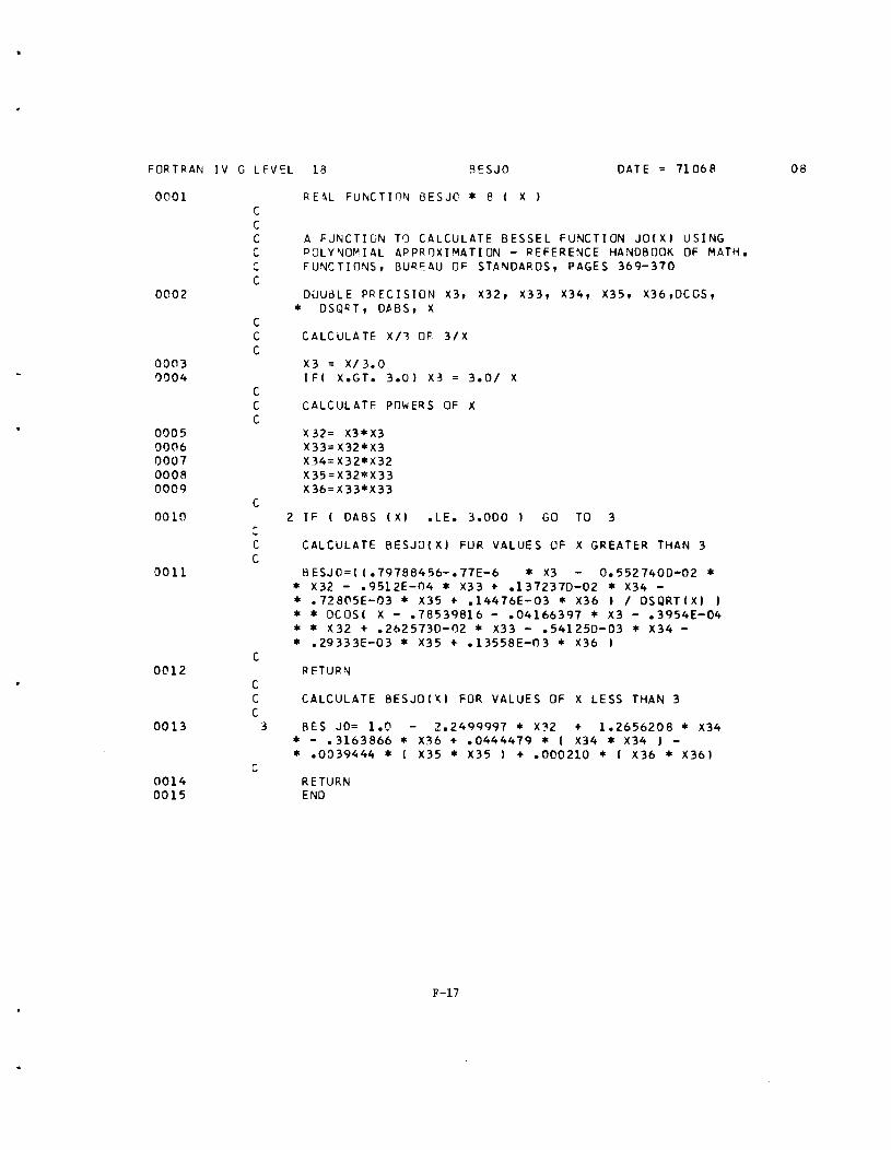
FORTRAN

0001

0002

0003 0004

oa05 0006 0007 0008 0009

0010

0011

0012

0013

0014 0015

IV G LEV EL

C C C ~

'" ~ ... C

C C C

C C C

C

18 BESJO OAT E = 71 068

RE~L FUNCTInN BESJO * 8 X I

A FUNCTION TO CALCULATE BESSEL FUNCTION JO(XI USING POLYNOMIAL APPROXIMATION - REFERENCE HANDBOOK OF MATH. FUNCTIONS, BURfAU OF STANDARDS, PAGES 369-370

DUUoLE PRECISION X3, X32, X33, X34, X35, X36,DCOS, * DSQRT, DABS, X

CALCULATE xn OR 3/X

X3 = X/3.0 IF! X.GT. 3.01 X3 = 3.01 X

CALCULATE POwERS OF X

X32= X3*X3 X33=X32*X3 04= X32*X32 X35=X32*X33 X36=X33*X33

2 IF ( DABS (XI .LE. 3.000 I GO TO 3

C C

C

C C C

c

3

CALCULATE BESJO(X) FOR VALUES OF X GREATER THAN 3

BESJO=I(.79788456-.77E-6 * X3 0.5527400-02 * * X32 - .9512E-04 * X33 + .1372370-02 * X34 -* .72805E-03 * X35 + .14476E-03 * X36 I I DSQRT(X) ) * * DCOSI X - .78539816 - .04166397 * X3 - .3954E-04 * * X32 + .2625730-02 * X33 - .541250-03 * X34 -* .29333E-03 * X35 + .13558E-03 * X36 )

RETURN

CALCULATE BESJOIX) FOR VALUES OF X LESS THAN 3

BES JO= 1.0 2.2499997 * X32 + 1.2656208 * X34 * - .3163866 * X36 + .0444479 * ( X34 * X34 ) -* .0039444 * ( X35 * X35 ) + .000210 * ( X36 * X361

RETURN END

F-17

08

FORTRAN

OO~l

0002

0003 0004

0005 0006

0007

0008 0009

IV G LEVEL

C C

C C C C C C C C C

C C C C

C C C

C

18 V DATE = 11068

REAL FUNCTION V * 8 XN , XM I

DOUBLE PRECISION XN, XM, EXPM2M, EXPM4M, OEXP

V - A FUNCTION OF 'E2El', AND 'M' 'E2El' IS THE EVEl RATIO, TESTED FROM .001 TO 1000. 'M' TESTED USING VALUES FROM 0.0 TO 150. WHICH IS 10 * IR/HI

V APPROACHES 1 FOR LARGE VALUES Of M

V 1.0 IFI XM .GT. 30 RETUR N

CALCULATE EXPONENTIALS

EXPM2M DEXP I -2.000 * XM I EXPM4M= EXPM2M*EXPM2M

CALCULATE fUNCTION V fOR THE XN & XMl OR XM2 VALues

V = I 1.000 + I 4.000 • XN • XM • EXPM2M I -• I XN • XN • EXPM4M I I I t 1.000 - ( 2.000 • XN • • I 1.000 + 2.000 • XM • XM I • EXPM2M I + • (XN. XN • E XPM4M I I

RETURN END

F-18

08

LOC OBJECT CODE ADDRl ADDR2 STMT SOURCE STATEMENT

00000(" 1 COREIt START 0 2 ENTRV CORE :3 EXTRN IBCOM. 4 EXTRN FIOCS#

000000 5 USING *,15 000000 47FO FOOC OOOOC 6 CORE BC 15,*+12 000004 07000000 7 DC XL4' 0700000(' , 000008 C3D6D9C5 8 DC CL4'CORE' I)OOOOC 90E4 DI"OC OOOOC 9 STM 14,4,12(13) 000010 9823 1000 00000 10 LM 2,3,0(1) 000014 5833 0000 00000 11 L 3,0(3) 000018 CJ023 F090 00090 12 STM 2,3,BUFADR 00001C 411 0 F02F 0OO2E 13 LA 1,CORE2 000020 4130 F074 00074 14 LA 3,CLOAD 000024 0523 15 BALR 2,3 000026 98E4 DOOC OOOOC 16 LM 14,4,12(13' 00002A IBFF 17 SR 15,15 OOC02C 07FE 18 BCR 15,14

19 DROP 15 00002E 20 USING *,1 r)OO02E 5040 106E 0009C 21 CORE2 ST 4, SAVE4 000032 1841 22 LR 4,1 0OOO2E 23 USING CORE2,,-

24 DROP 1 000034 1810 25 LR 1,0 000036 910F 1001 00001 26 TM lCl),X'OF' 00003A 4710 4022 00050 27 BC 1, OUTPUT 00003E 5810 4076 000A4 28 L 1,VFIOCS 000042 4130 4046 00074 29 LA 3,CLOAD 000046 0523 30 BALR 2,3 000048 9823 4062 00090 31 LM 2,3,BUFADR 00004C 47FO 4036 00064 32 BC 15,RETURN 000050 9823 4062 00090 33 OUTPUT LM 2,3,BUFADR 000054 9240 2000 00000 34 MVt 0(2),X'40' 000058 0630 35 BCTR 3,0 00005A 0630 36 BCTR 3,0 00005C 4430 4040 Oa06E 37 EX 3,DMOVE 000060 4133 0002 00('102 38 LA 3,2(3) 000064 5840 406E 0009C 39 RETURN L 4,SAVE4 000068 IBI0 40 LR 1,0

41 DROP 4 00006A 47Fl 0006 00006 42 BC 15,6(1) 00006E D200 2001 2000 00001 00000 43 DMOVE MVC 1(0.2),0(2) 000074 44 USING *,3 000074 50FO 3024 00098 45 CLOAD ST 15,SAVE 000078 58FO 302: OOOAO 46 L 15,VIBCOM 00007C 9250 F04A 0004A 47 MVI 74(15) ,X'50' 000080 440F 004A 0004A 48 EX 0,74(15' 000084 9258 F04A 0OO4A 49 MVI 74U51,X'58' 000088 58FO 3024 00098 50 L 15,SAVE 00008C 07F2 51 BCR 15,2 000090 52 BUFAOR OS 2F 000098 53 SAVE DS F 00OO9C 54 SAVE4 OS F OOOOAO 00000000 55 VIBCOM DC A( I BCOM#)

F-19

l DC J BJ ECT CODE

OOOOA4 00000000

AQ~~l ADDR2 STMT SOURCE STATEMENT

56 Vf I DC S 57

F-20

DC END

A(FIOCSIt)

NOTE: Program printouts of sample problems will

be found in the main body of the report,

Tables 6a through 6g.

F-21

LrSTI~G OF QATA ChRnS FOQ SA~PLE PROBLEMS

1001711!:>ftzrs \1560 1 1 t= t.'I 16B1SBl , 2.5 5nMI 1

?OO~F AL COAT 0.') CU~D SANny GRAVEL '.2.0GR!=Y & BRWN SAND SUR

15f>O 1 '5n6~ , - ~ 19.~ 17.1 52.1 'H.l 1~.03

11)60 1 C;21~O , - ~ ." B.'" 1 7 .1 5' .1 ~'.1 7'.03 11560 1 '521~8 ? - a 41., 2B.3 49.1 30.1 6R.03 15~O 1 521~o ? - R 40. , ?o.3 4 0 .1 JO.1 61.03 15j:.,0 1 c21 F.-o 3 - A 3~.' 11.1 41.1 30.1 65.03 1'560 1 152168 "l. - B ." 1 • ." 11.1 4f..l ~0.1 61.03 1';"0 1 5216'1 4 - A 49.3 32.3 49.1 32.1 14.03 . , 1560 1 521 f> 8 4 - ~ 46.3 30.3 41.1 31.1 71 .• 03 15f>0 1 ~2168 '5 - A. 4~.'" 2q.3 50.1 34.1 77.03 1560 1 ",216<3 5 - ~ 4? ." BO.1 46.1 31.1 1'3.03

F-22

Lr~Tl~G O~ ~ATa C~QDS FOQ SA~PL~ PPOBLF~S

10017RIH~zn<: '8'24 ? '~N! ?776NRL 8.0 57.168 1

200SFllL (" '1ttT 0.'; ASPHALT STAB. GPAVH 7.5GRFY SANOY CLAY SUBG

2R?4 2 £;?168 1 - a. C; 5.3 40.3 ;:>9.~ 66.1 50.1 21=174 Z '5?16~ 1 - B "2.3 37.3 e1.1 61.1 4Q.l 28?4 2 "?168 2 - A 77.3 49.~ 31. .3 71. .1 53.1 2874 2 cpl"'A, 2 - B 77.3 47.3 30.3 67.1 ';, .1 2824 2 "?l6R 3 - A ~1.3 ')0.3 31 • " 67.1 49.1 2824 2 S?16~ 3 - B A3.3 51.3 ':11. :3 67.1 50.1 2B:?4 2 5?16R 4 - A A3.3 49.3 30." 64.1 48.1 2824 2 1:i?}6R 4 - 13 81.3 47.3 28.3 61.1 47.1 2824 2 '5116R 5 - A 78.3 4R.3 29.3 62.1 45.1 2874 2 5?16R '5 - B 81.3 49.3 31.3 65.1 47.1

F-23

LISTT~~ ~F "ATA CARDS FOR SAMPLE PROBLEMS

1 0017 BU~ L FsnN 13qq 1 11="1 1361EBl 12.0 52168 1

ZOOC;E=AL Cr"lH 0.5 LI ~F. STAB. SANDSTnNFl1.5TAN SANOY CLAY SUBGR

13qq 1 521 f-R '. - A 1:i0.3 :'1. '3 71.1 47.1 33.1 139 q 1 ~216E1 l - R 52.3 41.3 78.1 48.1 33.1 13qo 1 5216fl ? - A !:i5.3 40.3 67.1 40.1 81.03 13qq 1 52168 ? - B 48.3 '35.3 64.1 38.1 82.03 13 QO 1 52168 ~ - A !:i0.3 35.3 60.1 37.1 Sc;J.03 13qq 1 52168 3 - B 48.3 33.3 58.1 'H.l 87.03 1399 1 52168 4 - A 1;0.3 35.3 56.1 34.1 12.03 139q 1 5216R 4 - B 46.3 :n.3 54.1 33.1 71.03 1399 1 52168 5 - A 64.3 42.3 65.1 40.1 28.1 139q 1 52163 5 - B "0.3 38.3 63.1 42.1 31.1

F-24

llSTI~G OF nATA CARDS FOR SAMPLE PROBLEMS

1001 7WASHPJGHlN lAb IS ISH ~6 NRL 19.9 52168 1

?OOH()T ~IX ASPH. CnI'.JC. ~.755AN[')$TONE 1615BLACK CLAY SUBGRADE

lA6 5 t; 7168 1 - A 56.3 )4.3 61.1 42.1 30.1 1~6 5 52168 1 - B 61.3 36.3 61.1 42.1 31.1 IA6 '5 C;?]~B ? - A 513.3 36.3 67.1 47.1 ~6.1 1M. 5 r;?]6~ ? - B [''i.3 39.3 69.1 49.1 37.1 186 5 5?168 ~ - 1\ '56.3 36.3 613.1 50.1 38.1 186 5 52168 ~ - "7.3 36.3 61.1 48.1 31.1 lA6 5 '5n6R 4 - A 56.'3 31.3 15.1 57.1 46.1 1 RI, 5 521~R 4 - B 52.3 3A.3 1~.1 55.1 44.1 186 ., 5?t68 5 - A 50.3 H.3 59.1 44.1 33.1 1 R6 Ii 52168 5 - B C::3.3 33.3 1,1') .1 43.1 33.1

F-25

1 001 7on~ I:'D n:(,),,1 4q A IllS lQO ~IBl 1 f;. 2 52168 1

?OOHOT ~IX A~ OH. (n~l( • 1.25(1;1>1. STlIB. lIMFsrnNE1395o F.D SANDY CLAY SUBGQ

4Q ~ r:;216A 1 - A 68. J 59.J 49.1 39.1 31.1 4q A 521~~ 1 - q "'3.1 60.1 49.1 39.1 31.1 40 A 15211..1:1 ~ - ~ 7.,.1 61.1 51 .1 39.1 31.1 40 8 521~A

., - q 70.1 f, ?. 1 49.1 39.1 31.1 49 A "2168 ':\ - ~ 7". , 65.1 52.1 39.1 30.1 49 A 152168 1 - B 76.1 6".1 51 .1 39.1 30.1 49 FI "i21"8 4 - ~ 60.1 54.1 45.1 35.1 28.1 4Q 0 521Ml 4 - ? "i ~.1. 52.1 4~.1 -:n.l 8~.1

49 FI 5Z16 A '5 - ~ /I-, ?. 1 55.1 4".1 35.1 91.1 49 A 5216? 5 - Ft "'':;.1 '57.1 47.1 36.1 28.1

F-26

LI~TI~G OF ~aTa (aqos F0Q SAMPLE PQOBLEMS

1 OOl1RIH, lOS 1560 1 1P~ 1681NBL 1.5 5216A I

200ASPHAL T ~IJQHC tNG 1.0 aC)DH FMUl STAB GPAVL 6.5FJROWN CLAY SUBGRAOE

15AO 1 521 ~B 1 - A 72.3 50.3 32.3 66.1 52.1 1560 1 "2168 1 - F\ 71.3 1)1.3 32."3 65.1 51.1 1561) ] 5211,A ~ - ~ 64.3 41.3 31.3 64.1 4q.l 15f.0 1 "216A , - 8 62.3 45.3 30.3 63.1 50.1 \560 1 "2t6F! 3 - A 68.3 4q.3 31.3 63.1 4q.l 1560 I r;216R ~ - R 6q.1 50.3 32.3 65.1 50.1 It;60 1 521 ~A 4 - A 14.3 54.3 34.~ 61.1 4q.1 1560 1 '521 bA 4 - B 14.3 5'3.3 34.3 65.1 4q.l 1S:;~o 1 "2168 I) - A f.6.3 46.3 10.3 61.1 41.1 1'560 , 1)21 6e 5 - B 66.3 4~.3 31.3 61.1 46.1

F-27

LISTr~G OF DATA ChRDS FOR SAMPLE PROBLEMS

, OO178 D AlOS 540 3 '~M Q14 ~BL 8.3 52168 1

700S'=-AL COAT 0.5 IRON aR~ GQ. AVEL 1.8GREY SANDY CLAY SUBG

540 :3 9' 68 , - A ~0.3 51.3 32.3 68.1 50.1 540 ~ 5'-'68 , - B 75.3 48.3 30.3 63.1. 48.1 540 '3 57' 68 2 - A 59. :3 30 .3 82.1 60.1 48.1 540 3 5?' 68 ? - R 60.3 40.3 82.1 62.1 49.1 540 ~ 5?"68 3 - A 55.3 39.3 28.3 64. '. 51.1 540 3 5?168 :3 - B 53.3 3q.3 2A.3 61.1 51." 540 '3 52168 4 - A 15.3 49.3 33.3 15.1 60.1 540 ~ 5?'.M 4 - B 78.3 53.3 35.3 79. , 63.1 540 3 5?'6R Ii - A 74.3 49.3 33. ~ 11.1 55.1 540 3 52'6~ 5 - B 10. :3 41.3 32.3 68.1 53.1

F-28

,