Z

R. & M. No. 3561

M I N I S T R Y OF

%',i:~ ,~ %

T E C H N O L O G Y ' :"~%

AERONAUTICAL RESEARCH COUNCIL

REPORTS AND MEMORANDA

Calculation of Subsonic Flutter Derivatives for Arrowhead Wing with Control Surfaces

By Dor i s E. Lehrian

Aerodynamics Division, N.P.L.

a n

LONDON: HER MAJESTY'S STATIONERY OFFICE 1969

PRICE £1 3s. 0d. NET

Calculation of Subsonic Flutter Derivatives for Arrowhead Wing with Control Surfaces

By Doris E. Lehrian Aerodynamics Division, N.P.L.

a n

Reports and Memoranda No. 3561"

March, 1967

Summary. An oscillatory lifting-surface theory for subsonic flow (Ref. 1) is used to calculate the aerodynamic

forces on an oscillating arrowhead wing of aspect ratio 2 with trailing-edge control surfaces of varying span. The collocation method is outlined for simple harmonic motion of arbitrary mode and frequency and is applied for modes of plunging, pitching and control rotation. The discontinuous upwash in the control-surface problem is replaced by a smooth equivalent function. An alternative treatment for total forces, such as lift and pitching moment, is provided by the reverse-flow theorem with collocation solutions calculated for the 'reversed wing' in appropriate modes.

Values of the aerodynamic derivative coefficients are presented for a range of frequency at the Mach numbers 0.781 and 0.927. The variation of the pitching derivatives with frequency, Mach number and pitching axis is illustrated and shows good agreement with the results obtained by other collocation theories and by low-frequency wind-tunnel measurements. For the control-rotation mode, the calculated values of the indirect control derivatives indicate the good comparisons between the various methods of constructing equivalent upwashes and also the satisfactory comparison with the other collocation theories. Values of the direct control derivatives appear more sensitive and large variations in magnitude are associated with the different collocation methods and equivalent upwash treatments.

CONTENTS

1. Introduction

. Acum's Lifting-Surface Theory

2.1. Collocation solutions for the load distribution

2.2. Calculation of generalized forces

. Plunging and Pitching Oscillations

3.1. Formulation of upwash and force modes

3.2. Reverse-flow relations for lift and pitching moment

. Control-Surface Oscillations

4.1. Reverse-flow treatment of lift and pitching moment

4.2. Construction of equivalent upwash function

4.3. Direct-flow treatment of hinge moment

5. Results for Plunging and Pitching Derivatives

*Replaces N.P.L. Aero. Report 1230~A.R.C. 29 047.

. Results for Control-Surface Rotation

6.1. Comparison of equivalent upwashes

6.2. Indirect control derivatives

6.3. Direct control derivatives

7. Concluding Remarks

. Acknowledgements

Notation

Definitions of Derivatives

References

Appendix A : Construction of equivalent upwash function appropriate to Acum's theory

Appendix B : The Function of Appendix A in the Limit ~ ~ 0

Appendix C : Construction of a simplified equivalent upwash function

Appendix D : A direct modification to the exact upwash

Tables 1 to 7

Illustrations--Figs. 1 to 20

1. Introduction.

This investigation considers linearized theoretical methods of evaluating flutter derivatives for general wing and control-surface configurations in subsonic flow. Although the methods are applicable to elastic modes of deformation, rigid modes are chosen for the purposes of direct comparison with experimental aerodynamic data. The present application is to the calculation of derivatives for simple harmonic plunging, pitching and control rotation of an arrowhead wing with trailing-edge controls of arbitrary span. The planform of aspect ratio 2 with a leading-edge sweepback of 60 ° is illustrated in Fig. la with half-span outboard controls.

The calculations are based on the subsonic lifting-surface theory developed by Acum (Ref. 1) for oscillating wings of finite aspect ratio. This method is an extension to general frequency of Multhopp's methods for steady flow 2 and low-frequency motion 3. Acum's method of obtaining collocation solutions for the load distribution over the wing is outlined in Section 2.1. The subsequent calculation of generalized forces for arbitrary modes is considered briefly in Section 2.2. The application to plunging and pitching modes is formulated in Section 3.1. The reverse-flow theorem due to Flax 4 provides an alternative way of determining the lift and pitching-moment derivatives (Ref. 5). Reverse-flow relations for these deriva- tives in terms of the plunging and pitching derivatives for the 'reversed wing' are given in Section 3.2.

Methods of evaluating control-surface derivatives by means of collocation solutions are considered in detail in Section 4. The reverse-flow approach can be applied to continuous force modes such as lift and pitching moment (Section 4.1). On the other hand, it is an advantage if the forces corresponding to the wing oscillations and to the control-surface oscillations can be computed from direct-flow solutions. The control-surface problem is therefore transformed to one with a continuous boundary condition. On a general reverse-flow basis, Davies 6 has constructed smooth equivalent upwashes for oscillating part-span controls; this three-dimensional approach, dealing simultaneously with the chordwise and spanwise discontinuities in upwash, is applied in Section 4.2 with a modification consistent with Acum's lifting-surface theory. This treatment leads to the rather complicated formulation given in Appendix A. Values of the equivalent upwashes appropriate to solutions for the arrowhead wing with controls are

discussed in Section 6.1 and are compared with values by the simpler methods formulated in Appendices B, C and D.

The reverse-flow basis of constructing equivalent upwashes depends upon the assumption that the force modes are smooth. In the case of forces such as hinge moment, no lifting-surface method deals rigorously with the discontinuities in both the upwash and force modes. Some methods use a distinct construction for equivalent upwashes appropriate to hinge moment, as for example in Ref. 7 for low- frequency oscillations where chordwise and spanwise discontinuities are treated separately. It is important to investigate and assess the merits of available treatments in the determination of the direct control- surface derivatives'(Sections 4.3 and 6.3).

Various collocation solutions for plunging, pitching and control-rotation oscillations have previously been evaluated for the arrowhead planform. For low frequency, results by the Multhopp-Garner method (Refs. 3 and 7) are available for the wing with control surfaces of different spans. For general frequencies, Davies '6 lifting-surface method has been applied for the particular control span shown in Fig. la and Woodcock 8 has investigated the accuracy of the solutions by considering various combinations of the chordwise and spanwise collocation positions. A link between low-frequency and general-frequency results is provided by the formulae from Ref. 9, that express the rate of change of a damping derivative with frequency in terms of appropriate quasi-steady stiffness derivatives for the same planform and Mach number. A limited number of results from wind-tunnel tests are available for subsonic flow. Derivatives for pitching oscillations at small frequencies have been measured at M = 0.8 and' M = 0.9 (Ref. 10) and for M > 0.5 (Ref. 11). The calculated and measured derivatives from all these sources are discussed in relation to those presented in this report for plunging and pitching motion in Section 5 and for control-surface oscillations in Sections 6.2 and 6.3.

2. Acum's Liftino-Surface Theory. The method of Ref. 1 is valid within the limitations of linearized theory for a thin wing describing

simple harmonic oscillations of small amplitude in a uniform subsonic free-stream. The integral equation between the load and upwash distributions is made tractable in Ref. 1 by an extension of the Multhopp lifting-surface methods of Refs. 2 and 3. Section 2.1 sets out the basic equations required to calculate the load distribution over a wing oscillating in an arbitrary mode. The calculation of the generalized forces is outlined in Section 2.2.

2.1. Collocation Solutions for the Load Distribution. The integral equation relates the complex upwash distribution w(x,y)e i°~ and the non-dimensional

load distribution l(x,y)e i~t over the wing planform assumed to lie in the plane z = 0. In the present notation equation (25) of Ref. 1 becomes

w(x,Y)u 8rclf f l(x'y')K(x°'y°)dx'dy'' (1)

S

where

X o = X - X ' , Y 0 = Y - Y ' ,

l(x,y) = lift per unit area/½pU 2 ,

U = free-stream velocity

and S is the area of the wing planform. The kernel function is defined by

xo

( i ~ o ) K ( x o , Y o ) = l i m o f ~3 z io9 exp z--* ~ S z 2 { l e x P [ U ~ ( ~ ° - M r ° ) ] } d¢° (2)

where ro = [~o2+/~ 2 yo2+/~ 2 z2] ~,

M = Mach number of the free-stream,

= [1-M2]~.

The use of a modified upwash ~ and a modified loading l, defined by

and w(x,y) = ff~(x,y) exp ( - kox/U)

l(x,y) = -l (x,y) exp ( - ie)x/U) ,

(3)

(4)

simplifies the integral equation (1). This equation is then reduced to a practical form for computation by extending to general frequency Multhopp's 3 'influence function' approach for low frequency. The particular features of this approach are the use of N chordwise terms in the load distribution, with their corresponding 'influence functions', and the N chordwise and m spanwise collocation positions on the planform where the upwash is evaluated.

Acum specifies the load distribution by equation (4) with an assumed series for the modified loading -l(x,y). In general,

N

q = l

in terms of the chordwise functions

F cos (q - 1)~b + cos q~b 1 %(4) = L i q-~os ~ cot ½ 4

_ [ cos (q - 1)~b+cos qq5 1 - m s i ~ j ' q = I(1) N , (6)

where the chordwise parameter ~b is defined by

x = x , ( y ) + ~ c(y) [1 - c o s O] (7)

and xz(y), c(y) are respectively the ordinate of the leading-edge and the local chord at the spanwise section y. In equation (5), Fq(y) are the unknown spanwise functions to be determined by a collocation solution of equation (1).

For the load distribution l(x',y'), each chordwise term q~q(~b') has an 'influence function' defined as

0

where the kernel function K(xo, Yo) is given by equation (2) and Xo = x - x ' , Yo = Y-Y'. The evaluation of equation (8) is reduced to a practical computation by means of an expression derived

in Ref. 12 for the kernel function K(xo,Yo). The influence functions can be expressed in terms of four non-dimensional parameters :

the Mach number M, the local frequency parameter [co c(y')/U], co-ordinates Ix - xt (y')]/c(y') and [fl(y- y')]/c(y').

The substitution of equations (2) to (7) into equation (1) leads to an equation for the modified upwash ,~(x,y) that is expressed in terms of the influence functions Fq(x,y,y') of equation (8). Hence

~(x,y) s

U 2re

N

- s . q = l

(9)

The spanwise integration with respect to y' in equation (9) is effected by the Multhopp interpolation technique of Ref. 2. The unknown spanwise functions Fq(y') are represented by polynomials in terms of their values F~. at the m spanwise stations y', defined by

[ I y',/s=~/,=sin un/(m+l) , n = T 1 (10)

where m is an odd integer. Thus,

n = ~ ( m - 1)

Fq(y) = ( -1 ) ~("+t) 2 Fq. n = - ~ ( m - i )

(_ 1),+ 1 sin(m+ 1)0 sin 0,

(m+ 1) (cos0-cos 0,) ' (11)

where y/s = t /= cos 0 and 0, = cos 0,. The modified upwash N(x,y) of equation (9) is now calculated at each collocation position (Xp~,y~) where the chordwise positions are defined by

t [1 - cos Cp] ] Xpv = Xlv~Cv ., p = 1(1) N, (12)

~)p [2pzc/(ZN + 1)]

and the spanwise positions are

y~/s=~v=sinlzcv/(m+l)l ,v= ( ~ ) ( 1 ) ( - ~ 2 I ) (13)

By equations (9) to (13), the modified upwash ~(x,,,,y~) is obtained in terms of the influence functions Fq(xp~,y~,y'.) corresponding to the spanwise station y', and the collocation position. Thus,

N

q = I

n=-~(m- 1)

+ E ' Fqn n = - ~ ( m - l )

[b Fq(xp y y')l } v n v~ v~ n (14)

where the dash on the summation sign indicates that the term n = v is omitted from the summation.

n

In equation (14),

b.. = 1)/II-,.')' i] I b,, = (1 -q,z)~'/[(m+ 1) ( t6 -q02] , Iv-hi = 1, 3, 5 . . (•5)

= 0 , I v - h i = 2,4,6

Furthermore, Fq(Xp~,y,y'~) denotes the particular form of influence function when n = v, which includes an additional contribution from the integration of equation (9) through the logarithmic singularity at y' = y as described in Ref. 1.

The evaluation of ~(Xp~,yO for a swept wing is modified by using the 'Multhopp interpolated wing' (Ref. 2, Section 5.3). For example, the kinked centre section of the arrowhead wing in Fig. la is replaced by the rounded planform shown in Fig. lb; the actual values at the spanwise station y = 0,

i.e., xt(0) = and c(0) = cr,

are replaced respectively by

X,o = x. 1 1 and Co = ~c,+-~cl

(16)

in terms of the values x~l and ca at the spanwise station y/s = sin [n/(m+ 1)].

Equation (14) for ~(xp~,y~) at the mN collocation positions, defined by equations (12) and (13), gives a set of linear simultaneous equations in the unknown coefficients

Fq, f o r q = l ( 1 ) N , n = ( ~ ) ( 1 ) ( - ~ ) .

These coefficients are determined for any oscillatory motion by satisfying the corresponding boundary condition at the positions (xw,y~). Assume a mode of oscillation j such that the upward deflection of a point (x,y) on the wing is, in complex notation,

z(x,y,t) = zj(x,y) bj e i°'' (17) where bj is the non-dimensional amplitude of the oscillation with angular frequency 09. The corresponding upwash must satisfy the tangential flow condition given by

w(x,y) e i°' = wj(x,y) bj e i°~t ]

wj(x,y) [- io9 O -1 I " (18) L-u J zj(x,y)

Hence, ~(xp~,y~) of equation (14) must satisfy the boundary conditions given by equations (3) and (18) at the collocation positions (xp~,y,) of equations (12) and (13). The loading coefficients -~,r(~)corresponding to modej are thereby determined and the spanwise load distribution F~ j) is then defined by the interpola- tion polynomial of equation (11). With equations (4) to (6), the required load distribution over the wing is obtained in the form

l(x,y) e ~°" = l~(x,y) b j e ~°~t . (19)

2.2. Calculation of Generalized Forces. The generalized aerodynamic force corresponding to a non-dimensional force mode f~(x,y) and the

load distribution of equation (19) is defined as

= f f sah-,~, FORCE ½ p U 2 b j e i° ' t f~(x,y) Ij(x,y) dx dy = pU 2 .v.,ij vj e .

S

(20)

When the series for li(x,y) from equations (4) to (6) is inserted, the non-dimensional force coefficient Qii is

N

= 4s2 (y) ] f ff,(x,y)[Zvq( )r? S q = l

By equations (6) and (7), the transformation to co-ordinates ~b and ~/= y/s gives

1

A f N

q = l

X

× [ exp (i2 cos (o-i~c) ] dqS drl , (21)

where

= _ _ co c(Y)2u ' X = u [ Xt(y)+½ c(y) ] and A is the aspect rati° ° f the wing"

The arbitrary force mode i can be expressed as

A = ~ n~')(n) cos (r- 1)~ r = l

= 0

over area C

over area (S-C)

(22)

where the area C can be defined by ~bl 0/) ~< ~b ~< 4~2 (t/) and ~/o ~< t/~< t/c. Then, equation (21) becomes

N R ~/c

q = l r=l ~b

(23)

where ,~ = o~ c O , ) / 2 c ,

x = 2 [1 + {2 xt(y)/c(y)}],

and

(O2

4'1

[{cos ( q - 1) ~ + c o s q~b} cos ( r - 1) qS] [exp (i2 cos q~)] dq~. (24)

It is assumed that the spanwise loading F~ j) (y) is determined as a smooth continuous function of y whether the mode j is continuous or discontinuous. The evaluation of the spanwise integral in equation (23) is effected by using the values of the integrand at the positions q = ~/,, with F~q J) (tl,) = F~J, ~ from the solution of Section 2.1. Any discontinuities that might arise from the wing parameters such as xt, or c, are removed by using a rounded planform as defined by equation (16) and illustrated in Fig. lb for the centreline kink on the arrowhead planform. For a full-span control surface however, the kink in the hinge line at y = 0 should be retained in the calculation of hinge moment. In general, the integration with respect to q can be reduced to a summation with respect to n by means of integration factors p(1) appropriate to the force mode f~. Then, the force coefficient Qij of equation (23) can be expressed in the form

n = ½ ( m - 1) N R

4 exp ( - iKn) F(J) p(1) R(~) = -- --q, --. --r, T~q (2,,41,,q~z,) (25) n = - ½ ( m - 1 ) q = t v = l

where the subscript n denotes a value at ~/= ~/. and the parameters R, ~b t and ~b 2 are specified by the particular mode f of equation (22). The functions T~q are evaluated from equation (24) by means of a K D F 9 programme for the integral

(O

Hk(2,4)) = f cos k q~ exp (i2 cos q~) dq~.

0

(26)

In the case of total wing forces such as lift and pitching moment, to be denoted as modes i = 1, 2 respectively, f of equation (22) is a smooth, continuous function over the area C = S defined by q~l = 0, (])2 = ~, qb = -- 1,/']c = l. Thus, equation (24) reduces to

(27)

where Jk(2) is the Bessel function of the first kind and i = x /L- i - . Since the integrand of equation (23) is a smooth function, Multhopp's interpolation polynomial in equation (11) may be applied to the integrand over the range - 1 ~< t/~< 1 to give integration factors

= cos ~ - ~ for m o d e s i = l a n d 2 . (28)

As an example, the lift force is defined by f = 1, R = 1 and B, (° = 1 in equation (22). Then, equations (25) with (28) give

n=½(m- 1) N

Q 1 J - 4 ( 2 A 1 ) 2 2[F~exp(-ix")c°S(m~---~l)T~q(2~'O'z)? (29,

n = - ½ ( m - 1) q = l

with Ttq(2,,0,rc) defined by equation (27) with r = I. Similarly, for the pitching moment about x = 0

when f2 = x/~, n=½(m- 1) N

Arc F(~ exp ( - i~,) cos ~ x Q2j = 4(m+ 1)

n= - ~-(m- I) q= 1

(30)

For a discontinuous force mode f , as implied by equation (22) when the area C 5~ S, the integral of

equation (23) is transformed to the variable 0 = cos - 1 t/where the positions 0, = cos- 1 q, = 2 m + 1

are at equally spaced intervals. To determine the integration factors p(0, the integrand is assumed to be a quadratic function of 0 over each double interval 0, ~< 0 ~ 0,+2. In general, the spanwise limits of integration t/b and t/c, in equation (23), do not coincide with positions 0,. For the particular case of the hinge moment on a full-span control, when t/b = --1 and t/c = 1, the procedure reduces to Simpson's rule over the whole wing span.

3. Plunging and Pitching Oscillations. In the case of a smooth continuous mode j, the load distribution 12(x,y) over the wing and the generalized

forces Qu are calculated by a straightforward application of Acum's theory as outlined in Section 2. When the force mode i is also a smooth continuous function of (x,y), an alternative evaluation of Qu can be made by applying the reverse-flow theorem 4. Such a calculation can be expressed in terms of collocation solutions for the 'reversed wing' oscillating in appropriate smooth modes s. For plunging and pitching oscillations, relations for the lift and the pitching moment are formulated in terms of the same force coefficients for the reversed wing (Section 3.2).

3.1. Formulation of Upwash and Force Modes. In the modes of plunging (j = 1) and pitching about an axis x = 0 (j = 2), the wing deflection is defined

by equation (17) with

zl = -~ , bl = Zo/~ l ! (31)

z 2 = - x , b2 Oo J

where z 0 and 0o are respectively the amplitudes of the plunging and pitching oscillations and ~ is the geometric mean chord of the wing. Then, by equation (18), the upwash distributions corresponding to these modes

= u E- iq l

J w2 = ~ [ - 1 - it, (x /~) ] (32)

where the frequency parameter ~ = o)UU. The corresponding loading lj(x,y) for j ---: 1 and 2 are determined as outlined in Section 2.1 with an appropriate choice of re(N). The required total forces are the lift, the pitching moment about x = 0 and the hinge moment on the symmetrical outboard control surfaces (Fig. la). These forces are defined in terms of the non-dimensional force coefficients Qij by equation (20) with i = 1, 2 and I respectively where the non-dimensional force modesfi are given by

f ~ = l t

f z = x/~ and

f , = [X-- Xh(y)]/8

= 0

over area S (33)

over area C

over area ( S - C) (34)

where S and C are respectively the area of the wing and the area of the control surfaces. It then follows from equations (31), (33) and (34) that the forces for plunging and pitching are determined in the form

Lift = L = pU2 S [ Q l l (Zo/C)+ Q12 00] e i''t

Pitching moment about x = 0

= d g = - p U 2 S ~ [Q21 (Zo/~) + Qzz 0o] e i~t (35)

Hinge moment about x = xh(y)

= H = - p U 2 S ~ [QI1 (Zo/C)+Qi2 0o] e i'~t

The evaluation of the force coefficients Qij from equation (25) is discussed in Section 2.2; in the particular cases i = 1 and 2 this formula reduces to equations (29) and (30) respectively. The forces in equation (35) are expressed as aerodynamic derivative coefficients by means of equations (57) in the Definitions with Xo = 0. Furthermore, the derivatives for plunging and pitching oscillations about an arbitrary pitching axis x = Xo can be determined by using equations (58) in the Definitions.

3.2. Reverse-Flow Relat ions for Lif t and Pitehin9 Moment .

For smooth continuous modesf~(x,y) the force coefficients Qi~ can be evaluated by use of the reverse- flow theorem 4. By equation (11) of Ref. 5, the general reverse-flow relation for all modes i an d j is

where

S

F j(x,y) = wj(x ,y) /U ,

(36)

Li(x,y) e i'~' is the loading over the wing in reverse flow due to an upwash distribution

Wi(x,y) e i'°t = U fi(x,y) e i'°t .

In the application of equation (36), the frequency of oscillation o~ and the flee-stream Mach number M are the same in the direct-flow and reverse-flow problems. In the present application, the m o d e s f are

10

defined for i = 1 and 2 by equation (33) and the distributions wj are determined forj = 1 and 2 by equation (32). The corresponding forces Qu from equation (36) can be interpreted in terms of the same total forces on the 'reversed wing' in direct flow. As in Section 4.2 of Ref. 5, this conveniently leads to relations for the lift and pitching-moment derivatives for plunging and pitching about the axis x = 0 in terms of the same derivatives for the reversed wing in plunging and pitching about an axis 2 = 0. The co-ordinates (x,y,z) of the actual wing are related to the co-ordinates (~,~,~) of the reversed wing by

x = c r - ~ , Y= - 9 , z = ~ .

Therefore, by equations (39) and (40) of Ref. 5 with k = ~, x o = 0 and Xo = 0, the reverse-flow relations for the derivatives are

1~=1~ t I~ = i~

Io = mz + (cfl6) 1~ + 1~

l o = m~ + (cfl~) 1~-- (1/~ z) 7z

m~ + Io = ~ +1o

m~ + lo = Ne + 7o

and

(38)

mo+ (cda) lo + Io = mo + (c,/~) 7o + 70

(39)

mo+ (c,/6) Io - (1/92) to =mo + (er/5) 7o - (1/~ 2) 70

~i'he bar used over the derivative coefficients on the right-hand sides of equations (38) and (39) indicates that these quantities relate to the 'reversed wing' with pitching axis ~ = 0. Hence, if the plunging and pitching derivatives for the 'reversed wing' in direct flow are evaluated by the collocation method of Section 2, then the lift and pitching moment on the actual wing with pitching axis x = 0 are determined by equations (38) and (39).

4. Control-Surface Oscillations. In the case of oscillating part-span control-surfaces, denoted by the modej = J, the upwash distribution

ws(x,y) is discontinuous along the hinge line and at the spanwise sections y = + y,. The corresponding loading ls(x,y) over the wing would have similar singularities and these cannot be determined by the collocation method. However, for a smooth continuous force mode f~(x,y)the total force coefficient Qu can be estimated by means of the reverse-flow theorem (Section 4.1). Alternatively, the problem of determining Qu can be converted to one in direct flow with a smooth equivalent upwash w~(x,y) replacing the discontinuous upwash Ws(x,y) in the collocation solution. A basis of constructing the function w~ for arbitrary planforms is considered in Section 4.2. Although not strictly valid for the discontinuous force mode f~(x,y), this approach might also provide a useful approximate estimate of hinge moment (Section 4.3).

The wing deflection for control surfaces oscillating symmetrically is given by equation (17) with

zj = - E x - xh(y)]

= 0

bs = 4o

over area C

over area (S-C) l ' (40)

11

where 3o is the amplitude of the oscillation and C is the area of the control surfaces. For outboard trailing- edge controls, the area C is defined by

Xh(y) <~ X <~ xt(y) and Yu ~< [Y[ ~ s, (41)

where Xh(y ) is the leading edge and hinge line of the controls. By equations (18) and (40), the upwash distribution wAx,y) is

ws(x,y) = U [ - 1 - i~ { x - xh(y)}/~] over area C

= 0 over area (S-C) (42)

where wj has chordwise and spanwise discontinuities respectively along the line x = Xh(y ) and at the sections y = _ Ya. The required total forces are the lift, the pitching moment about x = 0 and the hinge moment as defined by the force modesf in equations (33) and (34) for i = 1, 2 and I respectively. Expressed in terms of the non-dimensional force coefficients Q~j by equation (20) with j = J, these forces are

Lift = L = p U 2 S Q1J 4o e i~''

Pitching moment about x = 0

= ./H = - p U 2 Sc Q2J 40 e i'~t

Hinge moment about x = Xh(y)

= H = - p U 2 Sc QIJ 4o e~'t

These forces can be expressed as aerodynamic derivati' Definitions.

(43)

coefficients by equations (59) and (60) in the

4.1. Reverse-Flow Treatment of Lift and Pitching Moment. The force coefficients Q~j for i = 1 and 2 in equation (43) can be evaluated by using the reverse-flow

relation of equation (36) with Fj(x,y) = Ws(X,y)/U determined by equation (42). Thus

c

(44)

where the load distributions Li(x,y), i = 1 and 2, over the wing in reverse flow correspond respectively to the upwash distributions W~ = Uf(x,y) defined by the functionsfa and f2 of equation (33). That is,

w~ = u }

W2 = U(x/a) (45)

As in Section 4.2 of Ref. 5, the distributions W i and Li can be expressed in terms of solutions for the 'reversed wing'. Transform equation (45) to co-ordinates (~,y) of the reversed wing as defined by equation (37). Then

W1 = (i/f) u31(~,y )

WE = (-- i/r~) [-u52(~,y ) + {(i/~)-- (G/c)} v~t (~,y)-] (46)

12

where kl(~,Y) and ]~2(X,.~), analogous to equations (32), are the respective upwash distributions on the reversed wing for oscillations in plunging and pitching about an axis 2 --- 0. The corresponding load distributions 7~(x,y) and 72(~,Y) on the reversed wing can then be combined linearly to give the distribution Li(x,y) for i = 1 and 2. When equation (44) is transformed to the co-ordinates (~,y), it is evident that the evaluation of Qu depends largely on the values 7~(~,~) over the area C near the leading edge of the reversed wing. This is the region where the collocation solution for 7i(2,y) is least reliable, and it seems likely that the reverse-flow estimates of Q1J and Q2s will lose accuracy as the control-surface area C is reduced. I t is noted also that the use of plunging and pitching solutions for the reversed wing introduces terms of order 1/92 in equation (46). For small values of 9 it is preferable to use equation (36) with LI and L2 from 'reversed wing' solutions for the upwash distributions of equation (45) with x = cr-f t .

4.2. Construction of Equivalent Upwash Function. Using a three-dimensional approach, Davies 6 constructs equivalent upwashes for an arbitrary wing-

control configuration, that give the same total forces on the wing in reverse flow as the discontinuous upwash Ws(x,y ). In general, an equivalent upwash function w~s(x,y) can be chosen to give the same general- ized force Qu as the reverse-flow relation of equation (36). Thus, for the upwash Ws(X,y) of equation (42),

DSJQ,j= f f f dx dy t (47)

where the load distribution Li(x,y) over the wing in reverse flow corresponds to the upwash distribution W~(x,y) = Ufi(x,y). To determine W~s(x,y) from the identity in equation (47) it is necessary to assume that IV//and L i are smooth continuous functions of x and y. The loading Li(x,y) can then be represented by a series of polynomial functions with singularities appropriate to the leading and trailing edges in reverse flow.

The equivalent upwash function w~s(x,y) is now constructed by the treatment, suggested in Section 4.3 of Ref. 5, as being the most appropriate for a swept planform and for application with Acum's lifting- surface theory. It is assumed that

wi(x,y)= tJ~e~s,g~(x/e)o,(n), s = l t = l

(48)

where the o- chordwise and z spanwise polynomials are defined as

gs(x/O = [x/~] s- 1, 1 (49) ! o

f~,(~/) = [sin t 0/sin 0] where r / = y/s = cos 0

The unknown coefficients Ess t in equation (48) are determined by using the identity from equation (47) with the loading Li(x,y) represented by the series

q=l v = l

(5o)

13

where [1 + cos 0] = 2 I x - xl(y)]/c(y).

The factor exp (io~x/U) in equation (50) is consistent with an application of Acum's theory of Section 2.1 to a free-stream velocity - U in the direction of the positive x axis. The chordwise functions q~q(O) ap- propriate to the loading in reverse flow are defined by equation (6) with ~b replaced by 0 ; the functions q~q(O) give the correct singularities in loading at the planform edges, with x = x~(y) acting as a trailing edge and x = xt(y ) as a leading edge because ~ = (n-~b). The spanwise polynomials f~v(t/) in equation (50) are defined similarly to those in equation (49). When equations (48) to (50) are inserted into the identity of equation (47), a set of az simultaneous equations is obtained for the unknown coefficients Es~ t of equation (48). The solution of these equations and the evaluation of wes(x,y) is outlined in Appendix A ; it depends upon the geometry of the wing-control configuration and the frequency of oscillation but is independent of the free-stream Mach number.

It is apparent from equations (A.1) to (A.5) of Appendix A that the inclusion of the exponential factor in the load distribution Li(x,y) of equation (50) does lead to a complicated calculation for W~s(x,y). Some simpler forms for the reverse-flow construction of the equivalent upwash function are formulated in Appendices B and C. Values of these different equivalent upwashes, appropriate to a solution for the arrowhead wing of Fig. 1, are compared and discussed in Section 6.1.

4.3. Direct-Flow Treatment of Hinge Moment. By applying the reverse-flow theorem 4 to the second line of equation (47), it follows that the force

coefficient Qis can be determined from

S

(51)

where les(x,y) is the load distribution over the wing in direct flow due to the equivalent upwash distribution we~(x,y) of equation (48). The evaluation of les(x,y) and Qis is therefore effected by applying the collocation method of Sections 2.1 and 2.2 respectively. In particular, the distribution l~s(x,y) is determined in the form of equations (4) and (5) by solving the modified upwashes in equation (14) for the boundary con- ditions as given by the equivalent upwashes w~s(xp,y~) and equation (3). That is, equation (14) is solved at the collocation positions (xp,yv) for the conditions

Ns(Xp,yv) = [W~s(Xpv,y~) exp (if~ xp~/O)] ,

The construction of the equivalent upwash function w~s(x,y) in Section 4.2, relies on the assumption that the upwash and load distributions in reverse flow,

i.e., W~ = Uf~(x,y) and Li(x,y) in equation (47),

are smooth continuous functions of x and y. Thus, equation (51) is valid for forces in continuous modes f , such as lift and pitching moment, but it is not strictly applicable to a discontinuous mode, as is the case for hinge moment defined in equation (43) with f1 from equation (34). For part-span controls, the mode f~ has spanwise discontinuities at y = _+y, that persist into reverse flow, even though it has a chordwise singularity less severe than that of wj. However, the evaluation of the generalized force Qis by the collocation method of Section 2 does require some approximate representation by smooth equivalent upwashes. It is thought that the calculation of QH by equation (51) could give a useful estimate of hinge moment. On the other hand, a direct treatment for equivalent upwashes is provided in Appendix

14

D by the modifications to the exact upwash Wj(Xpv,Yv). The different values obtained for the direct control derivatives, from the solutions for w}(xpv,yv) computed by Appendices A, B, C and D, are discussed in Section 6.3.

5. Results for Plunging and Pitching Derivatives. Acum's theory 1 as outlined in Section 2 is applied with collocation solutions re(N) = 15(3) to the

arrowhead wing in Fig. 1. For plunging and pitching oscillations about the axis x -- 0, the aerodynamic derivative coefficients are calculated for the Mach number M = 0-781 at the frequency parameters

= 0.25, 0.50, 1.0 and for M = 0.927 at rv= 1.0. The derivatives for lift, pitching moment about x -- 0 and hinge moment on the outboard control surfaces of span ( s - Ya) are defined according to the formu- lation in Section 3.1 and equations (57) in the Definitions. These lift and pitching-moment derivatives are presented as Solution (1) in Tables 1 and 2 for the plunging and pitching modes respectively; the hinge moment derivatives for both modes are listed in Table 3 for values of the control-span parameter Ya/S = ~1~ = O, 0.25, 0"50 and 0.75. Alternative theoretical results, tabulated in Tables 1 and 2 as Solutions (2) and (3), are determined respectively by Acum's theory with the reverse-flow relations of Section 3.2 and by Davies' theory 6. Various aspects of the results are illustrated in Figs. 2 to 9 and are discussed in conjunction with the pitching derivative Values obtained from wind-tunnel measurements at low fre- quencies10'11.

Comparison of the direct-flow and reverse-flow solutions in Tables 1 and 2, indicates only small discrepancies between the lift and pitching-moment derivatives obtained by the two methods of calcula- tion. Satisfactory agreement does not establish the accuracy of either solution as has been discussed in detail in Section 6.1 of Ref. 5. The present collocation solutions re(N) = 15(3) probably give reasonable accuracy, although the discrepancies, and hence possibly the inaccuracies, increase with frequency parameter ~ and also with Mach number M.

The results given for ~ ~ 0 in Tables 1 to 3 are calculated to first order in frequency by the Multhopp- Garner theory 3 with re(N)-- 15(3). The distinction between the theories of Refs. 1 and 3 when ~ 0 arises from the treatment of the kernel function K ( x - x ' , y - y') of equation (2), when different forms of modified upwash and loading are taken, and this affects the numerical evaluation of the damping derivatives. However, it is seen from Tables 1 to 3 that the results for ~ ~ 0 by Ref. 3 do correlate satis- factorily with those for finite ~ by Ref. 1 in both the direct-flow and reverse-flow solutions.

The values of the plunging and pitching derivatives obtained by Woodcock s'l 3 from Davies' theory 6 with solutions m(N) = 12(4), are tabulated in Tables 1 and 2 for ~ = 0-01, 0.25, 0.5 and 1.0, the frequency parameter ~ -- 0.01 being denoted as ~ ~ 0. The theories of Acum 1 and Davies 6 are both developed from the Multhopp steady theory 2, but there are distinct differences in the two collocation methods. In particular, the number of spanwise collocation sections (m) is odd in Ref. 1 but even in Ref. 6. In the latter method, collocation positions do not occur at the centre section of a wing and it is therefore un- necessary to modify the arrowhead planform at the kinked section y = 0 by means of equation (16) as is required in Acum's theory. It is noted also that the total forces in Ref. 6 are evaluated by applying an interpolation technique to both the chordwise and spanwise integrations of the load distribution ; the forces could be more affected by the choice of N than in Acum's theory where the chordwise integration is exact by equations (24) and (25). Comparison of the lift and pitching-moment derivative values, given as Solutions (1) and (3) in Tables 1 and 2, does show significant differences between the two methods particularly for the Pitching damping derivatives l 0 and - r n o in Table 2; both solutions for M = 0.781 indicate a small effect of frequency for 0 ~< ~ ~< 1.

The variation of the plunging and pitching derivatives with the frequency parameter ~, the Mach number M and the pitching axis x -- x o is illustrated in Figs. 2 to 9. Unless otherwise stated, the results plotted are from the direct-flow solutions by Acum's theory [Solution (1)]. The derivatives for arbitrary pitching axis x -- x o are calculated by using equations (58) in the Definitions with derivatives for x o = 0 from Tables 1 to 3. In Fig. 2, the lift derivatives lz and leand the pitching-moment derivatives -mz and - m ~ for plunging motion at M = 0.781 are plotted against ~; for 9 < 1, the damping derivatives remain within about 2 per cent of the constant values for small ~ that follow from Ref. 9 with the low-frequency

15

solution. In Fig. 3, the stiffness derivative lo for pitching about the axis Xo = ½cr is plotted against M. Here, the ~ ~ 0 solutions provide a curve for 0 ~< M ~< 0.927, whilst the values of lo for ~ = 0.5 and 1 indicate a small but increasing frequency effect as M increases from 0.781 to 0.927. Similarly, Fig. 4 gives the damping derivative lo against M; for both axis positions Xo = ½cr and Xo = cr, the small effect of increasing ~ from 0 to 1 is of opposite sign at the two Mach numbers M = 0.781 and M = 0-927. For these values of M, the direct pitching derivatives -m o and -m o for the axes Xo = ½cr and Xo = c, are plotted in Figs. 5 and 6 against frequency parameter over the range 0 ~< ~ ~< 1. Again, the frequency effect is small but the results indicate a larger variation of - m o with ~ at the higher Mach number M = 0.927. The damping derivatives for small f are estimated from the ~ ~ 0 solution by using equations (18) and (19) of Ref. 9 which give the slopes as

(53)

By contrast, the slope of the stiffness derivative Omo/~?9 is zero as ~--* 0. The corresponding dashed lines of - mo and - rn o for small ~ < 0.4 are shown in Figs. 5 and 6 respectively, and these correlate very satis- factorily with the curves for ~ > 0.2 from Acum's theory at M = 0.781.

The variation of the pitching moment derivatives with axis position Xo is illustrated in Figs. 7 and 8 respectively by the values of - m o and -mo at M = 0.781 plotted against Xo/~ where the geometric mean chord ~ = 0'619 cr. Apart from the ~ ~ 0 solution 3, the results plotted are for ~ = 0.5 and these show the comparison between the direct-flow and reverse-flow solutions by Acum's theory and the solution from Ref. 13 by Davies' theory 6. Agreement is regarded as satisfactory in view of the differences in these collocation solutions as discussed above. The results show a similar rate of change of the derivatives with axis position, and -mo in Fig. 8 gives positive damping for all axes.

Measurements of the pitching derivatives for the arrowhead wing have been made in wind-tunnel tests for small values of the frequency parameter ~ < 0'14 and subsonic Mach number (Refs. 10 and 11). For lo and lo, in Figs. 3 and 4 respectively, the values 'experiment r~ ~ 0"085' at M = 0.8 and M = 0.9 are obtained by taking an optimum average over the measured range 0 ~< 9 ~< 0'11 of the results for 'Wing E' in Ref. 10. Comparison of the values for lo shows that theory is about 7 per cent higher than experiment but both give a similar variation with M. Likewise, for lo, in Fig. 4, low-frequency theory and 'experiment ~ ~ 0"085' show a similar variation with M, but here the theoretical values are some 25 per cent higher• For the direct pitching derivatives against 9 in Figs. 5 and 6, the measured values from Ref. 10 are plotted for ~ ~< 0.11 and M -- 0.8. While for - t o o in Fig. 5 the comparison with theory is good for both pitching axes, only for the axis Xo = cr is there satisfactory correlation for - mo in Fig. 6. The measured values of -mo for the axis Xo = ½c, show a rather large decrease in damping over the small range of ~?, a variation that seems unreliable. Discussion in Ref. 10 of the measurements for the damping derivatives suggests that 10 and -m o could be subject to tunnel interference effects, the degree of which is not established. Wind-tunnel data from two sources, Refs. 10 and 11, provide experimental values of -mo and -m0 at four axis positions in Figs. 7 and 8 respectively; the values from Ref. 10 are an optimum average over 0 ~< ~ ~< 0.113 of the measured values at M = 0.8, whereas the measured values from Ref. 11 correspond to ~ = 0.138 at M = 0"781. In Fig. 7, these values of - t o o indicate a smaller rate of change with axis Xo/C, than the calculated derivatives, but this is compatible with the lower ex-

• perimental value for lo at M = 0.8 in Fig. 3. In Fig. 8, the experimental and theoretical values for - mo are in fairly good agreement, except for the axis position Xo = 0-808~ = ½cr as already illustrated by the results from Ref. 10 in Fig. 6.

A final diagram for the pitching mode at M = 0.781, in Fig. 9, shows the theoretical values of the hinge-moment derivatives - h o and - h o plotted against ~ for part-span control surfaces qa = y, /s = O, 0"25, 0"50 and 0"75 as defined in Fig. 1. The curves for - ho show a similar frequency effect when t/, ~< 0.5, but less variation with ~ for the smallest outboard controls t/, = 0.75. The damping derivative - h o

16

increases less rapidly with 9 as t/a increases. For small frequencies, the hinge-moment derivatives are estimated from the 9--*0 solution a with the following formulae derived from equations (12) and (17) of Ref. 9,

ha = (ho)~-~o

A ha = (ho)v--,o q--i-6 9 (I o ho)~o

(54)

These results are shown by the lines of small-dashes for - ha when 9 ~< 0.2 and for - ha when 9 ~< 0.4 in Fig. 9, which give fairly good first approximations for each value q,. Also shown in Fig. 9 are curves of -ha and - h a against 9 for r/a = 0"5, calculated in Refs. 8 and 13 by Davies' theory 6. These results are slightly lower than the values by Acum's theory, the largest differences occurring at 9 = 1.

6. Results for Control-Surface Rotation. For the arrowhead wing with oscillating control surfaces of span ( s - y , ) defined by Fig. la, the control

derivatives are evaluated for t/, = y,/s = 0, 0.25, 0.50 and 0.75 with the same combinations of frequency parameter 9 and Mach number as used for the plunging and pitching derivatives in Section 5. The colloca- tion solutions re(N)= 15(3) by Acum's theory of Section 2 are obtained for the rounded planform shown in Fig. lb. In the case of the full-span control t/Q = 0, the straight hinge line is retained in the calculations. Each collocation solution is determined by equating the modified upwashes ff~(xw,y 0 of equation (14) to those obtained from equation (3) for an equivalent upwash function w~(x,y) appropriate to the values of t/~ and 9. • ~ . . . .

The construction of the function w~(x,y) by the reverse-flow treatment appropriate to Acum's theory, is independent of Mach number but is non-linear in frequency (Section 4.2 and Appendix A). In Section 6.1, this function is compared with the different w~(x,y) obtained as linear functions of 9 by the simpler procedures of Appendices B, C and D. The discussion of the corresponding solutions for the indirect control derivatives in Section 6.2, includes the correlation with low-frequency solutions by the method from Refs. 3 and 7 and the comparison with results from Refs. 8 and 13 by Davies' theory 6. Furthermore, alternative solutions for the lift and pitching-moment derivatives, by the reverse-flow relations of Section 4.1 with Acum's theory, provide results that do not rely on any equivalent upwash procedure. The usefulness of determining the direct control derivatives by means of functions w~(x,y) is discussed in Section 6.3, comparison being made of the values calculated for finite 9 according to Section 4.3 and for Y ~ 0 by a distinct treatment appropriate to hinge moment 7.

6.1. Comparison of Equivalent Upwashes. The particular case (t/Q = 0'5, 9 = 1) is selected to illustrate the equivalent upwashes W~s(Xp~,y~) used

in the collocation solutions for part-span control surfaces on the arrowhead wing. In the reverse-flow approach of Section 4.2, w~s(x,y) is defined as the double series in equations (48) and (49) in terms of a chordwise and • spanwise polynomials and the unknown coefficients Es~t, s = l(1)a, t = 1(1)-c; the coefficients are determined by means of equation (47) with the loading L~(x,y) represented by a series with aT terms, as for example in equation (50). The choice of the integers ~r and v is arbitrary, but it seems appropriate to take • = m = 15 and ~ = N -- 3 to correspond to the number of terms in the collocation solutions.

Values of w~s(xp,yv) at the collocation positions (Xp,yO defined by equations (12) and (13) with re(N) = 15(3), are evaluated as detailed in Appendix A. The values obtained with T(a) = 15(3) are tabulated in Table 4 as method (a). In Fig. 10, the values of Rl[w}(x3~,yO]/U and lm[w~s(x3~,yO]/U9 are plotted against the spanwise parameter t/ = t/v , v = 0(1)7, to show the variation of w.} along the line p = 3 that defines the collocation positions closest to the trailing edge and downstream of the hinge line in Fig. lb. For comparison, values of the exact upwash wAx,y ) from equation (42) along the line p = 3 are plotted for 0 ~< q ~< 1 in Fig. 10. It is seen that the high order polynomial series for w}(x,y) when ~ = 15, gives a marked drop across the discontinuity in w s at q = t/, = 0.5, but leads to some fluctuations in the values

17

wej(x3v,y~) a t the outboard collocation positions. On the other hand, if only ~ = 7 spanwise polynomials are used in equation (48), the corresponding spanwise distributions are very smooth, as shown by the curves in Fig. 10, but these give a poorer representation in the neighbourhood of 1/= ~/, and elsewhere. It seems therefore that the values W~s(Xp,yO given by ~ = 15 are the better choice.

The equivalent upwash functions w~a(x.y) constructed according to the methods (b), (c) and (d) of Appendices B, C and D respectively, are illustrated by the other sets of values w~(xp,y~) in Table 4 for the case (r/, = 0.5, ~ = 1) with m(N) = 15(3). The methods (b) and (c) are based on simplified forms of the reverse-flow approach in Section 4.2 and give weS(x,y) as a linear function of the frequency parameter ~. Although method (b) is the limiting form of method (a) as ~ ~ 0, comparison of the corresponding values in Table 4 indicates the fairly small effect of neglecting terms of 0(92) in method (b), even at 9 = 1. In method (c), a simplified load distribution is assumed for Li(x,y ) in equation (47), similar to that in Davies' procedure 6, and this gives the same Rl[w~] as method (b) but a distinct formtLJ,,~ for lm[wes]. As seen from Table 4, the differences between the values lm[wes(xp,yO]/U by methods ib) and (c) are small for p = 3 and relatively larger at the forward chordwise positions p = 1 and 2. As an alternative approach, method (d) retains the exact upwash wj(x,y) of equation (42) at all collocation positions (xp,y~) except those nearest to the chordwise and spanwise discontinuities in Ws. At each of those positions, a value w~s(x~,y~) is determined by modifying wj to be a simple continuous function of control-surface geometry (Appendix D). The values of w~s(xp,y~) from method (d) are the easiest to compute and essentially different from those of the other methods in Table 4. In Fig. 11, the four methods are illustrated by the values of

R l[w~(x,y,)]/U and Im[w~(x,y4)]/U

at the collocation section y4/s = r / 4 = 0.7071, plotted against the chordwise parameter ~ = Ix-xt(yg)]/c(y4). The curves for methods (a), (b) and (c) show that the series from equation (48) with z(a) = 15(3) does not resemble the exact discontinuous upwash wj(x,y4), but serves to determine the total forces of lift, first and second pitching moments as implied by the reverse-flow construction. At the collocation positions (xp4y4) , p = 1(1)3, corresponding to ~ = 0.188, 0.611 and 0.950 in Fig. 11, the values w~ from method (d) are identical to the exact upwash Ws except for the value Rl[w~] at ~ = 0.611; at this position, the Im[w}] is taken equal to the exact value because the distribution Im[wj] is continuous across the hinge line.

From the point of view of computation, the major part of method (a) is programmed but the calculation of input data is laborious and must be repeated for each value ofg. Method (b) requires less initial computa- tion but requires the solution of simultaneous equations to first order in frequency. Method (c) is the simplest to programme with a fairly simple calculation for the input data. The choice between these three reverse-flow constructions of w~s(x,y) depends finally on the analysis of the corresponding solutions for the control derivatives. The simplest construction for w~ is by the direct-flow method (d). It is likely to be less accurate for lift and pitching moment than methods (a), (b) or (c), but these have little advantage over method (d) for the evaluation of hinge moment (Section 6.3).

6.2. Indirect Control Derivatives. Values of the lift derivatives, le and l~, and the pitching-moment derivatives, - m e and -m~, defined

according to equations (59) in the Definitions, are given in Tables 5, 6 and 7 for the various combinations of the parameters ~,. f, and M. The results presented as Solutions (1 a), (1 b). (1 c) and (ld) are the direct-flow solutions corresponding respectively to the equivalent upwashes wej(xp,.,y~) from methods (a), (b), (c) and (d); solution (2) is calculated according to the reverse-flow treatment of Section 4.1. These solutions for the particular case (qa = 0.5, ~ = 1, M = 0.781) are tabulated in Table 5 together with some results from Ref. 8. For the various combinations (r/a , ~), Table 6 gives the Solutions (la), (lc), (ld) and (2) for M = 0.781, whilst Table 7 gives the Solutions (la) and (2) for M = 0.927. The variation of the indirect control derivatives with the frequency parameter ~, the Mach number M and the control-span parameter qa is illustrated in Figs. 12 to 17 by the results from Solutions (la) and (2).

18

The similarity in the equivalent upwashes W~s(Xpv,y~) of methods (a) and (b) for (t/. = 0"5, ~ = 1, M = 0"781) is reflected in the good agreement between the corresponding values for the indirect control derivatives in Table 5. On the other hand, the quite large differences between wes(xpv,yv) from method (a) and the simpler method (c)i in Table 4, have only a small effect on the corresponding derivative values of Table 5. Thus, Solution (lc) gives indirect control derivatives comparable with those determined in Solutions (la) and (lb) from the more complicated functions w~ of methods (a) and (b). The equivalent upwashes W~s(Xp~,yO of method (d), however, give the rather different derivative values of Solution (ld) although these are of the same order of magnitude as the other direct-flow solutions. The alternative reverse-flow calculations, Solution (2) in Table 5, show noticeably lower values for the stiffness derivatives l¢ and - m e but similar values for the damping derivatives l~ and - m~.

Inspection of the results presented in Table 6 indicates that the above comparisons for (r/, = 0.5, = 1) apply for all combinations of qa and ~ at M = 0-781. Thus, the indirect derivative values from

Solutions (la) and (lc) are very close, whilst Solution (ld) gives consistently lower values for the stiffness derivatives and higher or less negative values for the damping derivatives. However, there are larger discrepancies for l¢ and - m e between these solutions and the Solution (2); the latter values are lower by from 2 to 4 per cent as the parameters (~,, ~) increase. In contrast, the values of l~ and -m~ from Solution (2) fall within the scatter produced by the other solutions. The damping derivatives are numeric- ally small giving a large percentage s~eatter, but the maximum numerical discrepancies are rather smaller in magnitude than those for the stiffness derivatives. For M = 0.927 in Table 7, comparison of the indirect control derivatives from Solutions (la) and (2), shows discrepancies of similar magnitudes at this higher Mach number.

The accuracy of a collocation solution depends upon the theoretical method adopted and upon the number and location of the collocation terms and positions used in the solution. In Ref. 8, Woodcock compares various solutions re(N) by Davies' theory 6 and tentatively indicates that this method with m t> 8 and N >t 4 gives the generalized forces for rigid modes to within 10 per cent accuracy for wings of moderate aspect ratio. Control derivatives in Ref. 8 are determined by using equivalent upwashes based on the separate treatment of the chordwise and spanwise discontinuities by means of two-dimensional and slender-body theories respectively. Values of the indirect control derivatives from Ref. 8, tabulated as Solution (3) in Table 5, show the fairly small effect of changing re(N) from 12(4) to 20(4) in the solution for (t/~ = 0.5, ~ = 1, M = 0.781). The collocation method and equivalent upwash treatment of Ref. 8 are different to those of this report, and it is encouraging to find that all the direct-flow solutions in Table 5, i.e. Solutions (1) and (3), give similar results for the indirect derivatives. Values of the stiffness derivatives are 1 e = 0.27 and - m e = 0.47, implying a maximum variation of 4 and 2 per cent respectively. Comparisons for the damping derivatives appear less consistent, but these values are numerically much smaller with variations of similar magnitude to those for the stiffness derivatives.

The dependence of the indirect control derivatives upon Mach number M and frequency parameter is illustrated in Figs. 12 to 14 for the outboard controls defined by t/, = 0.5. The values denoted as

'method of Section 4.2' are the results of Solution (la) in Tables 6 and 7 ; those plotted as 'Woodcock' are the solutions re(N) = 12(4) for Wing E from Refs. 8 and 13. The low-frequency (~--.0) results are obtained from solutions by the theory of Ref. 3 with equivalent upwashes 7 determined by two-dimensi~nal theory with spanwise factors to allow for part-span controls. In Figs. 12 and 13 respectively, the values le and l~ plotted against M show the variation of the lift derivatives for the range 0 ~< M ~ 0.927 at particu- lar values ~ ~< 1. The curves through Woodcock's values indicate a qualitative change in frequency effect for the higher Mach numbers. The different methods show similar effects of ~ and M but the corre- lation is not entirely satisfactory. In Fig. 14, the pitching-moment derivatives for M = 0.781 are plotted against ~ ~< 1. Here, the lines for ~ < 0.2 are determined similarly to equations (54) by the method of Ref. 9 from the ~ ~ 0 solutions; that is,

m{ = (m~)v-.o l

m~ = (m~)~2o + ~ ~ (i~ rno)~o

(55)

19

This estimate correlates satisfactorily with the present method at higher frequenciesl Woodcock's values for - m4 give a different frequency effect for 9 > 0.4. These numerically small variations are probably explained by a change in accuracy of the solutions as ~ increases (cf. Solutions 3 in Table 5).

The dependence of the indirect derivatives on the control-span parameter 0 ~< q, ~< 1 is illustrated in Figs. 15 to 17 for the various values of ~ at M = 0-781. The derivatives l~ and -m~ have a fairly small variation with frequency for all controls qa, as shown in Fig. 15 by the reverse-flow solutions of Section 4.1. The direct-flow results are slightly larger and cannot readily be shown on the same diagram since the discrepancies are similar in magnitude to the variations with ~. On the other hand, for the derivatives I~ and - m~ in Figs. 16 and 17 respectively, it is seen that the direct-flow results, by Section 4.2, ale System- atically lower than the curves of the reverse-flow values and the discrepancies are small. For ~ ~ 0, the corresponding solutions by the theory of Ref. 3 are obtained from the direct-flow treatment of Ref. 7 or the reverse-flow method in Ref. 5 ; the discrepancies are similar except for the full-span control ~/a = 0. The distinctive frequency effect on l~ and -m4 becomes larger as the control span increases, that is as qa decreases.

6.3. Direct Control Derivatives.

The hinge-moment derivatives -h~ and -he , defined according to equations (60) in the Definitions, are calculated from the direct-flow solutions with equivalent upwashes determined by methods (a), (c) and (d). Corresponding to these Solutions (la), (lc) and (ld) respectively, derivative values are tabula- ted in Table 5 for the case (ft, = 0.5, ~ = 1, M = 0.781) and in Table 6 for the various combinations (ft,, ,7) at M = 0.781; values by Solution (la) are presented in Table 7 for ~ = 1 and M = 0.927. The variation of the direct control derivatives with the control-span parameter, frequency parameter and Mach number is illustrated in Figs. 18 to 20.

Comparison of the different solutions for M = 0.781 in Tables 5 and 6, shows maximum variations less than 3 per cent for the values of -h~ and less than 10 per cent for the values of -h~ for all values of t/, and ~. The differences between Solutions (la) and (lc) are negligible for -h~ but show the maximum variation for -h4. By contrast, the direct method in Solution (ld) gives the largest values of -h~ whilst the values of -h~ are approximately an average of those from Solutions (la) and (lc). For the particular case (t/, = 0'5, ~ = 1), Table 5 also gives Solution (lb) and this is virtually the same as Solution (la). These comparisons suggest that each of the equivalent upwash methods could give an acceptable theo- retical estimate of the direct control derivatives, providing the collocation solution is sufficiently accurate. Woodcock's investigation 8 of the accuracy of various solutions re(N) by the collocation theory of Ref. 6, is instructive. His results for (q, = 0.5, ~ = 1, M = 0.781) by solutions with re(N) = 12(4) and m(N) = 20(4) are given in Table 5 as Solutions (3). These solutions give very similar values for - h e and -h 4 but the stiffness derivatives are smaller and the damping derivatives much larger than the values obtained by the present methods. It is noted again that the method of Ref. 8 uses a direct construction for equivalent upwashes and also an evaluation procedure for hinge moment based on equivalent displacements at the N chordwise loading positions. The poor comparison between the hinge moments from Solutions (1) and (3) suggests that the direct control derivatives are more sensitive to the method of calculation than the indirect derivatives in Section 6.2.

The variation of - h~ and - h~ with Mach number M and frequency parameter ~ is illustrated in Figs. 18 and 19 for the outboard controls defined by t/, = 0.5. The values denoted as 'method of Section 4.3' are the Solutions (la) of Tables 6 and 7; the results of Woodcock are the solutions m(N) = 12(4) for 'Wing E' from Refs. 8 and 13. Low-frequency results are calculated from solutions re(N) = 15(3) by Ref. 3, to correspond to the two types of equivalent upwash constructed for ~ -~ 0 in Ref. 7. The one based on the two-dimensional approach to total wing forces is similar to that used in Ref. 8, whereas the other is recommended in Ref. 7 for the calculation of hinge-moment derivatives. In the present application, the former equivalent upwash is chosen to give the two-dimensional forces of (CL, Cm, Cram), whilst the latter satisfies (CL, Cm, Cn). The corresponding solutions for the direct control derivatives are plotted in Figs. 18 and 19 as Ref. 7 (C,,m) and Ref. 7 (CH). In Fig. 18, these results for ~ ~ 0 provide curves against Mach number for the range 0 ~< M ~< 0.927 and show dissimilar estimates for - h~ but fairly good agree- ment for - hs. For finite ~, the results of the present method and Woodcock indicate a very small frequency

20

effect, but the two methods give differing estimates of the derivatives, in particular for the damping -he. Neither method shows a consistent correlation with the low-frequency results. Thus, Fig. 18 reveals again that the direct control derivatives, especially the damping at high subsonic M, vary considerably with equivalent upwash treatment and collocation method. This is clearly shown in Fig. 19 where the values -h~ and -h~ for t/a = 0.5 and M -- 0.781 are plotted against ~. The best correlation for -h~ is between the 'method of Section 4.3' and the ~ --* 0 value of Ref. 7 (C,,,,), but these solutions show the worst correlation for - he. As already noted in Section 5, the collocation methods of Refs. 1 and 3 when

~ 0 are formally different for the evaluation of damping derivatives. By contrast, in Fig. 19, Woodcock's values for -he are lower whereas those for -h~ are quite close to Ref. 7 (Cram). For these three methods the equivalent upwash construction is consistent, although it varies in detail; the variations in the derivatives probably arise mainly from the differences between the collocation methods. On the other hand, the distinct construction for hinge moment in Ref. 7 (Cu) produces a much lower result for -h~ but a very similar result for - h~ compared to Ref. 7 (Cm,,). In Fig. 19, the low-frequency values of Ref. 7 (CH) are extended to small ~ < 0.2 by means of equations (12) and (17) of Ref. 9, that is by

(he) = (h¢)~. 0 [ , (56)

A / (h~) = (h~)~o +]-~ ~ (1¢ ho)~.-~o

where the value (l~),-o is determined from the solution Ref. 7 (Cm,,,).

The variation of the direct derivatives with control span is illustrated in Fig. 20 by the curves of - h~ and -h4. against the control-span parameter 0 ~< t/, ~ 1, for various p at M = 0.781. The results by the method of Section 4.3, indicate a small frequency effect that increases as the parameter t/a decreases. The rapid increase in -h~ and -h~ as t/,--.0 can be attributed to the kinked hinge line, defined for the full-span control in Fig. lb. For ~---0, the distinct solutions of Ref. 7 (Cu) gives curves of -he and -h~ that are respectively much lower and much higher than the present method. However, all the results

in Fig. 20 indicate a similar rate of change of the direct control derivatives with qa.

7. Concludin 9 Remarks. (i) For the arrowhead wing A = 2, the plunging and pitching solutions by Acum's theory 1 with

re(N) = 15(3) are satisfactory. The derivatives show a fairly small effect of frequency over the range < 1 for subsonic flow M ~< 0.927. The comparison with wind-tunnel measurements 1°'1~ for low fre-

quencies is good except for the derivative lo referred to mid-chord axis. (2) The lift and pitching-moment derivatives calculated for plunging and pitching modes by the

reverse-flow treatment are in close agreement with the values from the direct-flow solutions. (3) For the control-surface mode, different equivalent upwash functions are determined by a reverse-

flow construction and these vary considerably according to the representation adopted. The corre- sponding solutions by Acum's theory show very small variations in the magnitude of the indirect deriva- tives and somewhat larger differences between the values of the direct control derivatives.

(4) Damping derivatives for small values of ~ are estimated by applying an expansion theory 9 to the solutions for ~-~ 0. For the lift and pitching moment due to plunging, pitching and control rotation, the frequency effect indicated by this method correlates very well with that by Acum's theory.

(5) Comparisons with the results by other theories reveal that the direct control derivatives vary considerably according to collocation method and equivalent upwash treatment. Although the frequency effect is consistently smaU, these derivatives show large variations (Figs. 19 and 20) and no assessment of accuracy is possible.

(6) A further investigation considering solutions for various re(N) would give useful information on accuracy. This would be facilitated by a single KDF 9 programme incorporating all stages of the com- putation.

(7) Further to the wind-tunnel tests for pitching oscillations in Ref. 10, the measurements for control derivatives will provide data for the hinge moment due to pitching motion and the direct and indirect

21

derivatives for control-surface oscillations. When these results are available, the need for further theo- retical work may arise.

8. Acknowledgements. This investigation was started under the supervision of Mr. W. E. A. Acum, now of Ship Division,

N.P.L. Mrs. S. Lucas of Aerodynamics Division and the DEUCE Section of Mathematics Division, NPL, were responsible for the basic collocation solutions. Further, the author wishes to acknowledge the later assistance given by Mathematics Division in the preparation of KDF 9 programmes. In particular, the equivalent upwash function was programmed by Miss S. M. How of Aerodynamics Division under the guidance of Miss B. Curtis of Mathematics Division. Miss How also helped with the analysis of results and Mrs. Lucas prepared most of the illustrations.

22

A

bj ~? (~)

c(y)

c:(y)

~f cr

ct

C

CL,Cm,Cmm, CH

Ejst

f,(x,y) F j(x,y)

Fq(x,y,y')

Fq(xp~,yv,y'.)

Fq(xpv,y~,y'd

os(x/~) hz,h~

ho,ho

he,he H

Hk(2,¢)

K(xo,Yo)

l(x,y)

7(x,y)

t~(x,y)

/~(x,y)

Iz,I~

~,~

NOTATION

Aspect ratio of wing planform [ = 4s2/8]

Amplitude of oscillation of wing for mode j

Polynomial function representingf(x,y), equation (22)

Local wing chord

Geometric mean chord of wing [ = S/2s]

Local chord of control surface

Geometric mean chord of control surface

Root chord of wing

Tip chord of wing

Area defining force mode, equation (22); area of both control Surfaces in case of hinge moment

Force coefficients of lift, first and second pitching moments, hinge moment respectively, for 2-dimensional control oscillating at ~ ~ 0

Coefficients determining equivalent upwash function, equation (48)

Non-dimensional displacement of force mode i

Non-dimensional displacement of mode j for wing in reverse flow

'Influence function' corresponding to ~q(¢'), equation (8)

Values of influence functions in collocation solution, equation (14)

Particular form of influence function when n = v

Chordwise polynomial of degree s, equations (48) and (49)

Hinge-moment derivatives for plunging mode

Hinge-moment derivatives for pitching mode

Hinge-moment derivatives for control rotation

Tail-down hinge moment about x = xh(y )

ChordMse integral defined by equation (26)

Kernel function defined by equation (2)

See

Definitions

Complex load distribution over wing, lift per unit area/½ p U 2

Modified load distribution by equation (4)

Load distribution corresponding to an upwash wi(x,y )

Load distribution corresponding to the equivalent upwashes wej(Xpv,Yv)

Complex load distributions on 'reversed wing' corresponding to the upwash ~i(~,Y)

Lift derivatives for plunging mode See Definitions

Lift derivatives for pitching mode

23

1~,I¢

L

Li(x,Y)

m

mz,m~

m~t,Yl't(j

M

ill

N

Qij

s

S

t

Trq(,~,~ 1,~2)

U

w(x,y)

~(x,y)

wJx,y)

w~(x,y)

W~(x,y)

x,y,z

x',y'

x0,Yo

(x~,.yO

Xo

Xh(Y)

xt(Y) x~(y)

Lift derivatives for control rotation. See Definitions.

Lift force on wing

Complex load distribution on wing in reverse flow, corresponding to upwash W~(x,y)

Number of spanwise terms or collocation stations

Pitching-moment derivatives for plunging mode ] See

Pitching-moment derivatives for pitching mode I Definitions

Pitching-moment derivatives for control rotation

Mach number of free stream [ = U/speed of sound]

Nose-up pitching moment about axis x = x o

Number of chordwise terms or collocation positions

Spanwise integration factors appropriate to mode i, for the evaluation of Qi~ by equation (25)

Generalized aerodynamic force coefficient, equation (20)

Semi-span of wing

Area of wing planform

Time

Chordwise integral of equation (22) required for the evaluation of Q~

Free-stream velocity

Complex upwash distribution on wing

Modified upwash distribution by equation (3)

Upwash distribution for wing oscillating in mode j, equation (18)

A smooth equivalent upwash function for mode j = J

Complex upwash distributions on 'reversed wing' where i = 1, 2, correspond respectively to plunging and pitching oscillations with axis ff = 0

Complex upwash distribution on wing in reverse flow [ = Ufi(x,y)]

Rectangular co-ordinates defined in Fig. la

Variables of integration in Section 2.1

(x -x ' ) , ( y -y ' ) in Section 2.1

Upwash positions in collocation solution, equations (12) and (13)

Rectangular co-ordinates for 'reversed wing', equation (37)

Location of pitching axis x = Xo (Fig. la)

Hinge line and leading edge of control surfaces

Leading edge of wing Trailing edge of wing

24

Ya

z(x,y,t)

zj(x,y)

Zo

fl r /y)

i-,(j) qn

q

qa

qb,q~

0

0o K

2

P

0 01,02

Op

%(0)

(D

Subscript i

Ordinate defining span of outboard control surfaces (Fig. la)

Upward deflection of wing surface

Upward deflection of wing in mode j

Amplitude of upward deflection in plunging oscillation

Compressibility factor = (1 - M 2 ) ~

Function representing the spanwise distribution of the q~h term in the reduced loading l(x,y) of equation (5)

Spanwise loading coefficient at ~ = ~/,, in solution for mode j

Non-dimensional spanwise ordinate (= y/s)

Parameter defining span of outboard control surface (= ya/s)

Parameters defining spanwise extent of area C in equations (22) to (24)

Spanwise collocation stations, defined by equation (10), (13) respectively

Angular spanwise ordinate (= cos- lq)

Amplitude of angular deflection in pitching oscillation (nose-up)

½ c(y)]/u

co c(y)/2u

co~/U

Non-dimensional chordwise parameter = [x-x~(y)]/c(y)

Amplitude of incidence of control, relative to wing, in control-surface oscillation

Free-stream density

Number of chordwise, spanwise polynomials in the function w~s(x,y) of equation (48)

Angular chordwise ordinate, equation (7)

Parameters defining chordwise extent of area C in equations (22) to (24)

2np/(2N+ 1) with p = I(1)N

Angular chordwise ordinate for 'reversed wing' (= re-0)

Chordwise function for the qth term of the series for 7(x,y), equations (5) and (6)

Chordwise function for the qth term of the loading Li(x,y) on the wing in reverse flow, equation (50)

Angular frequency of oscillation

Spanwise polynomials used in the construction for w~s(x,y) in Section 4.2 [equations (48) to (50)]

Denotes a force mode in direct flow and a deflection mode in reverse flow or for 'reversed wing'

Denotes a deflection mode in direct flow, and a force mode in reverse flow or for 'reversed wing'

25

I

J

n

P

q

/,

s

t

v

v

Superscript

Mode i = I denotes hinge moment

M o d e j = J denotes control-surface rotation

Denotes value at collocation station ~/= ~/.

Denotes value at chordwise position ~b = ~bp

Denotes a function or coefficient corresponding to the chordwise function q~q

Appropriate to r th term of polynomial representingf~ in equation (22)

Chordwise terms ~ denotes value corresponding to terms

Spanwise terms ~ of function W~s(x,y) in equation (48)

Denotes value corresponding to the spanwise function f~v

Denotes value at collocation station ~/= q~

A bar over a derivative coefficient indicates that the symbol relates to the 'reversed wing', as in equations (38) and (39).

26

DEFINITION OF DERIVATIVES

For plunging and pitching oscillations referred to an arbitrary pitching axis x = Xo, Fig. (la), the wing deflection is

z(x,y,t) = - [Zo + ( x - Xo) 0o] e i°'t •

The aerodynamic derivative coefficients for lift, nose-up pitching moment about x = xo and tail-down hinge moment are defined respectively by

L = p U 2 S [(/~ + i~ l~) (Zo/6) + (lo + i~ Io) 0o] e i°n /

= p U 2 S~ [(mz + if, m~) (Zo/~) + (mo + i9 mo) 0o] e i°" ] • (57)

H = p U 2 Cry [(hz + ff h,) (Zo/~) + (ho + i9 ha) 0o] e ~'°~

If the derivatives are known for the pitching axis x = 0, then the derivatives for any pitching axis x = Xo can be evaluated by using the following formulae: For the stiffness derivatives,

lz(xo) = Iz(O)

lo(xo) = lo(O)- (Xo/~)Iz(O)

m~(xo) = m~(0)+ (Xo/~)lz(O)

mo(Xo) = me(O) + (Xo/O)[lo(O)- m~(0)] - (x0/~) z Iz(0)

hz(xo) = hz(O)

ho(xo) = ho(O) + (Xo/O) h~(O)

(58)

For the damping derivatives, these formulae apply if the subscripts z,O are replaced by ~, 6). For the wing with control surfaces in Fig. (la), the symmetrical outboard control surfaces are of total

area C defined by xh(y) <~ X <~ xt(y), Ya <~ lYl <<- S. The control-surface deflection mode j = J is defined by equations (17) and (40). The corresponding forces of lift, pitching moment about x = 0 and hinge moment are expressed as aerodynamic derivative coefficients by the formulae

and

L = p U 2 S[l~ + if, l~] 4o e i'°t "~

J J/g= pU 2 S~[m~ + i9 m~] 40 e i~'t

H = pU 2 C~y [he+if, h~] 40 e~'°'

(59)

(60)

where 9 = mUU, ~ is the geometric mean chord of the wing, ~: is the geometric mean chord of the control surfaces.

For xo = 0, the lift L, pitching moment J¢ and hinge moment H are defined for deflection modes of plunging and pitching by equation (35) of Section 3.1 and for the control-rotation mode by equation (43) of Section 4, in terms of appropriate generalized forces Qo"

27

No. Author(s) 1 W.E.A. Acum

2 H. Multhopp ..

3 H.C. Garner ..

4 A.H. Flax ..

5 D.E. Lehrian and H. C. Garner

6 D.E. Davies ..

7 H.C. Garner and D. E. Lehrian

8 D.L. Woodcock

9 H.C. Garner and R. D. Milne

10 G.Q. Hall and L. A. Osborne

11

12

K. J. Orlik-Rtickemann and . J. G. Laberge

C. E. Watkins, H. L. Runyan and D. S. Woolston

13 D.L. Woodcock ..

REFERENCES

Title, etc. Theory of lifting surfaces oscillating at general frequencies in a

subsonic stream. A.R.C.R. & M. 3557. February 1959.

Methods of calculating the lift distribution of wings. (Subsonic lifting surface theory).

A.R.C.R. & M. 2884. January 1950.

Multhopp's subsonic lifting-surface theory of wings in slow pitching oscillations.

A.R.C.R. & M. 2885. July 1952.

Reverse-flow and variational theorems for lifting surfaces in non-stationary compressible flow.

J. Aero. Sci., Vol. 20, pp. 120-126. 1953.

Comparative numerical applications of the reverse-flow theorem to oscillating wings and control surfaces.

A.R.C.R. & M. 3488. August 1965.

Calculation of unsteady generalised airforces on a thin wing oscillating harmonically in subsonic flow.

A.R.C.R. & M. 3409. August 1963.

The theoretical treatment of slowly oscillating part-span control- surfaces in subsonic flow. (To be written).

On the accuracy of collocation solutions of the integral equation of linearized subsonic flow past an oscillating aerofoil.

Proceedings of the International Symposium on Analogue and Digital Techniques Applied to Aeronautics, Liege 1963, pp. 173-202. (1964).

Asymptotic expansion for transient forces from quasi-steady subsonic wing theory.

Aeronaut. Quart. Vol. XVII. November 1966.

Transonic and supersonic derivative measurements on the plan- forms of the Ministry of Aviation Flutter and Vibration Com- mittee's first research programme.

A.R.C. 26016. June 1964.

Static and dynamic longitudinal stability characteristics of a series of delta and sweptback wings at supersonic speeds. NRC, (Canada), NAE Aero Report LR-396. January 1966.

A.R.C. 28 435. October 1966.

On the kernel function of the integral equation relating the lift and downwash distributions of oscillating finite wings in sub- sonic flow.

NACA Report 1234. 1955.

Unpublished M.O.A. Report, 1962.

28

APPENDIX A

Construction of Equivalent Upwash Function Appropriate to Acum's Theory.

The reverse-flow basis of determining the equivalent upwash function weS(x,y) is outlined in Section 4.2. Thus, into the reverse-flow identity of equation (47) are inserted the discontinuous upwash wAx,y) of equation (42) and the smooth upwash function W~s(x,y) from equations (48) and (49). When the load distribution Li(x,y) in equation (47) is represented by the series of equation (50), the construction is consistent with a reverse-flow application of Acum's theory. From the resulting equation, the terms for each arbitrary coefficient %v of the series for Li(x,y) are identified; this gives a set of az simultaneous linear equations that can be solved for the unknown coefficients Ej~ ~ in the function weS(x,y) of equation (48). Hence

~ 2 dx dy {f f o, si, exp,,ox, , t s = l t = l S

dx dy

c

l (A.1)

1 with

where

and

q = l(1)a, v = l(1)z,

x = xt(y) +½ c(y) [ i + cos ~-1,

y = scosO

cos ( q - 1) O+cos q 0 Wq(~k) = sin O

Transform to the variables of integration (~O,0) and take

Dq~(O) = i [{xt + ½ c(i + cos ~k)}/e] ~- 1 [cos ( q - 1) ~k + cos qff] exp (i2 cos ~b + ix) d~b o

(A.2)

and

0h

6.(o) = f [ - 1 - i2 (cos ~k - cos ~h)] [COS (q-- 1) ~k + COS q~k] exp (i2 cos ~b + ix) d~k (A.3)

where

= co c ( y ) / 2 u ,

~c = 2['1 + 2 {xt (y)/c(y)}],

cos ~b h = - 1 + 2 [xh(y)- xl(y)]/c(y).

29

Since the wing and control-surface geometry is symmetrical in y, the integrals with respect to 0 in equation (A. 1) will be zero when (v_ t) on the left-hand side of the equation or (v_ 1) on the right-hand side is an odd integer. Thus, the set of equations from (A.1) reduce when z is taken as an odd integer to give

Ess t=O for s = l ( 1 ) a , t = 2 ( 2 ) ( z - 1 ) , (A.4)

and, by equations (A.2) and (A.3),

for

and

where

s = l t = l

~/2

f Dqs(O) sin vO sin tO dO } 0

Oa

t o

s = l(1)a,t = l(2)z

q = 1(1)~, v = l(2)z

cos 0 a = rla

(a.5)

The evaluation of the integrals in equations (A.5) is effected by using Simpson's rule with values of the integrands at the spanwise positions 0 = (rob~32) for b = 0(1)16. The upper limit 0~ does not in general coincide with any position k -- 0(2)16 and so modified integration factors are used to allow for this, (cf. calculation of hinge moment in Section 2.2). The calculation of the integrands in (A.5) therefore requires the values Dq~(b) from equation (A.2) and Gq(b) from equation (A.3). The integrations with respect to ~b in these two functions can be expressed in terms of the integrals Hk(2,O), by equation (26), with ~k = n and ¢ = ~O h respectively. The values of xt(y) and c(y) in 2,x and ~b h, are evaluated for the positions b to correspond to the rounded wing planform as defined for the collocation solution by equation (16). For the full-span control r/a = 0, the values xh(y) in ~b h are evaluated for the straight hinge line (Fig. lb).

A KDF 9 programme is available for the major part of the calculation of W~s(Xp~,y~). With the number of terms (a,z) specified in equation (48) for w~s(x,y), the programme requires as input data the values Dq~(b) and G~(b) corresponding to the particular case (r/,,r~) and also the integration factors appropriate to each side of (A.5). The programme calculates equations (A.5), forms and solves the set of simultaneous equations for Es~z. It evaluates wes(xp~,yO at the given collocation positions (xp,yO and also calculates the modified upwash ~s(Xp~,y~) required for the collocation solution by equations (14) and (52).

30

APPENDIX B

The Function of Appendix A in the limit f~--* O.

It is again assumed that the equivalent upwash function is represented by the series for wes(x,y) of equations (48) and (49). The unknown coefficients in-Ess ~ are determined to first order in frequency co by taking the limit of the reverse-flow construction of Appendix A as 9 -- o~UU ~ O. Thus, in equation (A.1), the exponential terms are expanded and all terms 0(e) 2) are neglected. It follows that Es~ are determined from equations (A.5) with the functions DqjO) and Gq(O) defined as

Dqs(O ) =

and

Gq(O) =

i ['(xl + 1 c (1 + cos ff)) /~] ,- 1 [cos ( q - 1) ~, + cos q ~O] x

o

× [1 +it¢ + i2 cos ~] d~

IJ/h

f I - 1 - ire- i2 (2 cos ~ - cos ~h)] [COS (q-- 1) ~ + COS q~k] d~k

0

(B.1)

The calculation of equations (B. 1) can be effected analytically and the spanwise integrations in equations (A.5) are then evaluated numerically as in Appendix A. The resulting set of simultaneous equations is linear in r~ and the solution for Esst is obtained generally by equating the real and imaginary parts to first order in frequency. It follows that w~(x,y) is a linear function of ~.

31

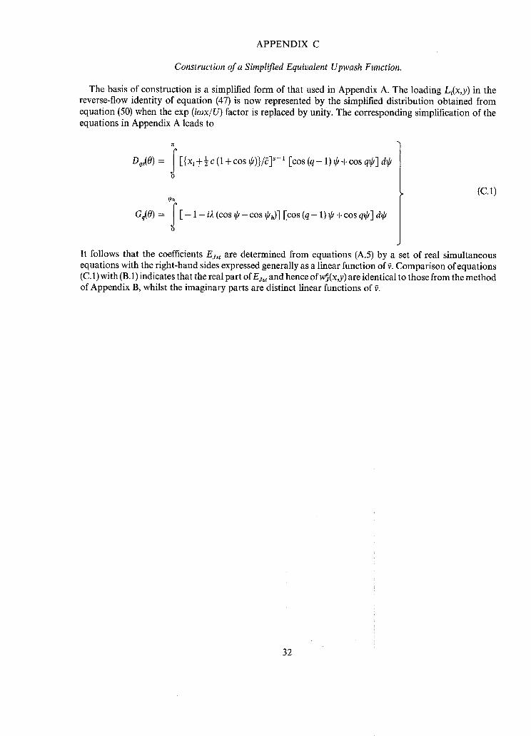
APPENDIX C

Construction of a Simplified Equivalent Upwash Function.

The basis of construction is a simplified form of that used in Appendix A. The loading Li(x,y) in the reverse-flow identity of equation (47) is now represented by the simplified distribution obtained from equation (50) when the exp (icox/U) factor is replaced by unity. The corresponding simplification of the equations in Appendix A leads to

Dqs(O) = i [{x, + ½ c (1 + cos ~0)}/8] ~-1 [cos (q - 1) ~ + cos q~] de 0

~h

Gq(O) = f [ - i - i2 (cos ~ - cos ~0h) ] [cos (q - 1) ~ + cos q@] d~k 0

(C.1)

It follows that the coefficients Ess ~ are determined from equations (A.5) by a set of real simultaneous equations with the right-hand sides expressed generally as a linear function of ~. Comparison of equations (C. 1) with (B.1) indicates that the real part ofE:s t and hence of w~s(x,y) are identical to those from the method of Appendix B, whilst the imaginary parts are distinct linear functions of ~.

32

APPENDIX D

A Direct Modification to the Exact Upwash.

This method of determining w~ is a direct procedure based on the values of the actual upwash Ws(x,y) from equation (42) in Section 4, namely

wj(x,y) = - - U I l +ff {x--xh(y)}/~ 1

= 0

over area C

over area (S-C)

(D.1)

where for the control surfaces in Fig. 1, the area C is defined by Xh(y) <<. X <<. xt(y ) and Ya ~ lyl ~< s. There is a chordwise discontinuity at the hinge line xh(y) and a spanwise discontinuity across each section y = +y, . Values ofw~s(X~,yv) at the collocation positions (xw,y~) of equations (12) and (13) are determined by treating these discontinuities independentty.

(i) Treatment of chordwise discontinuity. At each section y~, w} is to be determined for the chordwise collocation positions p = I(1)N. Denote

the hinge line by p = P,, so that by equation (12)

1 - cos 2N + 1 / = 2 c, / , let p** be the integer nearest to P,. (D.2)

It is assumed that

W~s(Xp~,y,) = Ws(Xp~,y,) when p = I(1)N excluding p = p*~,

but that

w~(xp~,y~) = Ws(Xp~,y~) + [p*~ +_ ½- P~] 6(PO when p = p*~,

(D.3)

(D.4)

where the + or - sign is selected to give [p*~+½-P,l ~ ½, and 5(PO is the increment in ws in crossing the discontinuity from P ~ - to P~+. If p** = P,, w~ is the average of the values ws(xp,,y 0 at p = P ~ - and p = P , + .

Applying equation (D.2) to the full-span control surface on the arrowhead wing, defined in Fig. lb for the collocation solution m(N) = 15(3), it is seen that p = p*~ = 2 is nearest to the hinge line p = P~ for all sections 0 ~< v ~< 7. Then, by equations (D.1), (D.3) and (D.4) with

/~ (PO = - U ,

w}(xl,,yv) = 0 ]

w~(x2v,yO = U(P~-2½) I w}(xa.y~) = Ws(X3,,,yO as given by (D.1)

(D.5)

33

(ii) Treatment of spanwise discontinuity.

For the spanwise discontinuity in Ws across the section y = ya, let v* be the integer nearest to

v = a = ( - ~ ) s i n - ~ ( ~ e ) . (D.6)

m-l) At each spanwise section y = y~, where v = 0(1) ~ includes v = v*, evaluate wej(Xpv,yv) as follows

for p = I(1)N :

when v < a , from equation (D.3) for all values p ' /

when v > a , from equation (D.3) for p @ p*~ ]

when v > a, from equation (D.3) for p = p*,

(D.7)

At v = v*, these values weAxp,y~) are modified by the addition of a correction term C}(p,v*) that allows for the spanwise discontinuity in wj across the section v = a. If p*, is the integer value p nearest to the hinge-line position P~ at v = a, then C}(p*,,v*) must incorporate the chordwise modification given by equation (D.4) for the chordwise discontinuity in wj at x = Xh(y a-b). Thus, when v = v*, the additional correction to weAx~,y.,) from equation (D.7) is

ceAp,V *) = [-V* __+ }-- a] A(p) for p =p p*, , (D.8)

but cej(p*a,V *) = [ v * ~ l _ a ] {A(P*a).q_rn, ~21 p"l (D.9)

where A(p) is the increment in wj in crossing the spanwise discontinuity at v = a; the + or - signs are selected to give Iv* + ½ - a I < ½ and [P*o + ½ - P ° I < ½. The corrections of equation (D.8)are applied when v* > a and v* < a. If v = v* --- a, it can be shown that the value of w s is given by the average of Ws(Xp~,yv) at v = a - and v = a + , with the addition when p = p*, of the correction [p*a+l--pa] (~(ea+).

For an outboard control Ya = ½ s and collocation solution re(N) = 15(3), as in Fig. 1,

equation (D.2) gives 2 < P~ < 2.5 and hence p*~ = 2 for all sections a ~< v ~< 7 ;

by equation (D.6), a = 8/3 and therefore v* = 3.

The upwash distribution wj is defined by equation (D.1) with the area C given by (p 1> P~, v >/8/3). The equivalent upwashes W~s(Xp,~,y,.) are then determined according to equation (D.7) with equations (D.8) and (D.9). Thus, by equation (D.1),

w3(xp.y~) = 0 if p = l o r i f v ~ < 2 ,

and w~(xp,yO -- - U [-1 + i~ (xp~- Xhd/g] ifp = 3 and v/> 4.

At the positions p = 2, by equations (D.4) and (D.1) and with P, from equation (D.2),

w~s(Xzv,yO = U[Pv-2½] ifv >/4;

34

with the correct ion from equat ion (D.9), for the posi t ion (19 = 2, v = v* = 3),

wes(xza,y3) = - U [-(2½- P3) + (2½- a) (2½- Pa)]

= U [Pa -2"472] since P , = ,2½.

F o r the posi t ion (p = 3, v = v* = 3) by equations (D.1) and (D.8),

w~(xaa,ya) = - U [1 + i~ ( x a a - Xh)/6] + [ . ~ ] A ( p = 3)

where

A(p = 3) = - U [ l + i ~ ( x 3 v - x h O / ~ ] with v = a = 8/3.

35

T A B L E 1

Lift and Pitching-Moment Derivatives for Plunging Mode.

- - m z

- - m ~

Solu- t ion* ~ 0

0 0 0

1 0

2 0 3 0

1.281 1.280

1"291

1 1.381 2 1.359 3 1-352

M = 0"781

= 0-25 ~7 = 0-5

- 0 - 0 1 7 - 0 . 0 8 1 - 0 . 0 1 8 - 0 . 0 8 5 - 0-021 - 0.094

1.268 1"260 1.268 1.260 1.281 1.278

- 0 . 0 2 8 - 0 - 1 2 5

- 0'029 - 0.128 - 0 . 0 3 2 - 0 . 1 4 1

1.368 1.362 1.346 1.340 1.342 1.342

~ = 1.0

- 0 - 3 7 1 - 0-388 - 0 - 4 1 5

1.294 1.299 1.338

- 0"548

- 0 ' 5 6 6 - 0 . 6 1 7

1.413 1.393 1 "429

~ 0

0

0

1"374

1.393

0

0

1.516

1-472

M = 0.927

9 = 1.0

- 0 . 2 2 8 - 0.245

1.333 1.368

- 0 - 3 8 8 - 0.421

1.532 1.546

T A B L E 2

Lift and Pitching-Moment Derivatives for Pitching Mode (Xo = 0).

M = 0-781 M = 0-927 Solu- t ion*

~ 0 ~ ~ = 1'0 ~--*0 ~ = 1'0

Io

lo

- - m 0

- - m 0

1 1.281 2 1.280 3 1.291

1 2.323 2 2.332 3 2.401

1 1.381 2 1.359 3 1.352

1 2.927 2 2.910 3 2.987

= 0.25 ~ = 0.5

1.261 1-211 1.259 1.208 1.271 1-220

2.351 2-374 2.360 2-383 2.431 2.457

1"344 1-246 1.322 1.221 1"313 1-209

2.959 2.994 2.941 2.977 3.024 3.070

1.020 1.015 1.054

2.428 2.445 2.538

0.879 0.845 0.851

3 . 0 8 4

3.078 3.228

1.374

1.393

2.356

2.502

1.516

1.472

3-150

,3.293

1-315 1.361

2.272 2-318

1.333 1.341

3.031 3.092

*Solut ion (1) = Theo ry of Ref. 1 with m(N) = 15(3), (Section 2). So lu t ion (2) = Reverse-f low solu t ions by Sect ions 4.1 and 2. Solu t ion (3) = Theory of Ref. 6 with re(N) = 12(4).

36

TABLE 3

Hinge-Moment Derivatives on Control Surfaces of Various Span tla, due to Plunging and Pitching Modes (Xo = 0).

M = 0.781

qa ~ 0 " ~ = 1"0

- - h z

-h~

-ho

- h ~

0 0.25 0.50 0.75

0 0.25 0-50 0.75

0 0.25 0.50 0.75

0 0.25 0.50 0.75

0 0 0 0

0.158 0.122

0.087 0-034

0.158 0.122 0.087 0.034

0.825 0.654 0.487 0.282

f = 0-25 ,7 = 0.5

- 0.020 - 0.083 - 0 . 0 1 6 - 0 . 0 6 7 - 0 . 0 1 2 - 0 . 0 5 1 - 0 . 0 0 8 -0 -033

0.161 0.173 0.123 0.129 0.087 0-088 0.033 0.033

0.132 0.060 0"097 0.025 0.065 - 0.001 0-018 -0 .03O

0.856 0.889 0.676 0.699 0.501 0.514 0.287 0.291

- 0 . 3 3 2 - 0"278 - 0 . 2 1 6 -0"139

0.240 0.168 0.102 0.034

- 0 . 1 7 9 - 0 - 2 3 6 - 0 . 2 5 6 - 0-222

1.004 0.791 0.568 0.310

M = 0"927

~-->0" ~ = 1"0

0 - 0"302 0 - 0"291 0 - 0"270 0 -0"197

0"194 0"346 0"137 0"264 0"079 0"164 0"008 0'036

0"194 0'057 0"137 -0"095 0"079 - 0'247

0"008 - 0"314

1"060 1" 140 0"815 0"985 0"562 0"768 0"276 0"404

*Method of Ref. 3 for ~ ~ 0.

37

TABLE 4

~e Equivalent Upwashes w s(xp,,,y,) Calculated by the Methods of Appendices A, B,~C and D for the Control-

Rotation Solution of the Arrowhead Planform when (t/, = 0.5, ~7 = 1) and re(N) = z(a) = 15(3).

Method

a

b

d

p = l p = 2 p = 3 v

R 1 I m R 1 I m R 1 I m

0 0-01518 1 -0.00039 2 -0.01684 3 0.08690 4 0.04987 5 0.13713 6 0.06348 7 0.16694

0 0-04192 1 -0.02108 2 -0-00103 3 0.07693 4 0-06143 5 0.13180 6 0"07109 7 0.16302

0 0"04192 1 -0.02108 2 -0.00103 3 0.07693 4 0.06143 5 0.13180 6 0.07109 7 0-16302

0 0 0 0 0 0 0

0"04985 -0 .03747

0.02452 0.00342 0.03010 0-02125 0-02049 0.02624

0.05551 -0.04088

0.02647 0'00269 0.03082 0.02128 0.02047 0-02652

0.02785 -0.01922

0.00982 -0.00891 -0.00938

0.00300 -0.01128

0.00940

0 0 0 0 0 0 0 0

-0-02512 +0.02956 -0.03445 -0.13597 -0.30366 -0.23955 -0.38534 -0 .32984

- 0.02076 + 0-02591 - 0-03145 - 0-13647 - 0"29999 - 0.24038 -0 '38313 - 0.33087

-0"02076 +0.02591 -0"03145 -0.13647 -0.29999 -0.24038 -0.38313 -0.33087

0 0 0

-0.14777 -0.20774 -0-24863 -0.29511 -0.33594

-0.00283 +0.00571 -0-00918 -0-00016 -0"03170 -0.00375 -0.03627 -0.00495

-0.00161 +0.00472 -0.00834 -0"00086 -0.03109 -0.00422 -0.03585~ -0 .00530

-0 '00174 0-00443

-0 .00720 0.01389

-0.00738 0.01070

-0.01493 0-00691

0 0 0 0 0 0 0 0

-0.01996 +0.01874 -0.01977 -0.77177 - 1.09548 -0.95712 - 1.07564 -0.98152

-0.02237 +0.02072 -0.02142 -0.77200 - 1'09819 -0.95706 - 1.07731 -0"98119

-0.02237 +0.02072 -0.02142 -0.77200 - 1.09819 -0.95706 - 1.07731 -0"98119

0 0 0

-0.83333 - 1.00000 - 1.00000 - 1.00000 -1.00000

-0.01532 +0.01502 -0"01555 -0.12346 -0.17415 -0 '10685 -0.12976 -0-08360

-0-01537 +0.01494 -0.01536 -0.12354 -0.17376 -0.10708 -0.12944 -0.08385

-0.00795 +0-00813 -0 .00894 -0-13552 -0.17561 -0.11894 -0.13041 -0.09468

0 0 0

-0.15657 -0.16134 -0.13784 -0.12037 -0.10962

38

TABLE 5

VariousSolutions~rtheDerivatives ~theControlSurfaces~a= ½0scillatingat~ = lwhen M = 0"781.

re(N)

15(3)

12(4) 20(4)

Solu- tion*

la lb lc ld 2

0.2767 0.2768 0.2770 0.2745 0.2665

0-2712 0.2673

-0"0244 -0.0249 -0.0252 -0.0212 -0-0226

-0.0250 -0.0279

- - m ~

0.4718 0.4724 0.4732 0.4662 0.4570

0.4681 0.4652

-m~

0"0037 0.0033 0.0032 0.0084 0.0037

-0.0032 0.0070

-he

0.4104 0-4118 0"4148 0"4222

0"3716 0-3697

-h~

0"1182 0'1178 0"1292 0"1252

0'1994 0'1953

*Solution (la) = w} of method (a) in Appendix A

Solution (lb) = w} of method (b) in Appendix B

Solution (lc) = w~ of method (c) in Appendix C

Solution (ld) = ~s of method (d) in Appendix D

Solution (2) =

Solution (3) =

Reverse-flow solutions in Section 4.1

Applied with the theory of Ref. 1 from

Section 2.1

Collocation method of Ref. 8 (equivalent upwashes in solutions by Davies' theory of

Ref. 6).

39

TABLE 6

Effect of Control-Span Parameter ~la and Frequency Parameter ~ on the Derivatives for Control-Surface Oscillations at M = 0-781.

0 0-25

0"25

0"50

0"50

1 '00

0"25

0"50

1"00

0"25

0'50

1.00

Solu- tion*

la lc ld 2

la lc ld 2

la lc ld 2

la lc ld 2

la lc ld 2

la lc ld 2

la lc ld 2

la lc ld 2

la lc ld 2

0.9314 0.9318 0.9250 0.9160

0'9184 0.9198 0.9129 0.9022

0.9034 0.9075 0-9005 0-8865

0-5791 0.5792 0.5736 0.5667

0.5696 0.5701 0.5646 0.5562

0.5536 0.5546 0.5501 0.5372

0.2984 0.2985 0.2947 0-2908

0-2919 0-2921 0.2886 0-2837

0.2767 0.2770 0.2745 0.2665

-0"0599 -0"0589 -0.0457 -0.0513

-0.0273 -0.0274 -0.0143 -0.0211

0.0161 0.0125 0.0265 0-0169

-0-0714 -0.0705 -0.0634 -0-0637

-0.0520 -0.0520 -0.0445 -0.0462

-0.0254 -0.0267 -0.0192 -0.0243

-0.0485 -0.0486 -0.0442 -0.0433

-0"0389 -0.0392 -0.0348 -0-0347

-0-0244 -0.0252 -0-0212 -0.0226

- - m ~

1"3460 1"3467 1-3357 1-3191

1"3342 1"3371 1"3254 1"3082

1"3206 1"3303 1"3163 1"2984

0'8905 0"8906 0"8795 0"8676

0.8830 0.8840 0.8728 0"8602

0"8710 0-8743 0-8631 0-8488

0"4901 0"4902 0"4821 0.4755

0"4849 0"4854 0"4774 0"4703

0"4718 0"4732 0"4662 0.4570

- m~

0"0670 0.0712 0"0833 0"0715

0"0996 0"1025 0"1147 0"1028

0"1358 0"1339 0"1479 0"1382

0"0023 0"0032 0.0122 0'0055

0"0212 0"0224 0"0306 0"0230

0'0424 0.0417 O'0502 0.0417

-0"0159 -0"0156 -0-0102 -0"0133

-0"0070 -0"0069 -0"0016 -0"0053

0"0037 0"0032 0.0084 0"0037

-he

0.6116 0.6124 0"6300

0.6206 0.6239 0.6396

0.6485 0.6608 0.6699

0.4655 0.4660 0.4768

0-4703 0-4721 0-4820

0.4864 0.4934 0.5000

0.4016 0.4018 0.4120

0.4034 0.4045 0.4141

0.4104 0.4148 0.4222

-h~

0.2117 0.2289 0.2192

0.2074 0.2237 0-2148

0.1834 0.1956 0.1898

0.1485 0.1618 0.1522

0.1466 0.1592 0.1503

0.1347 0"1456 0"1380

0.1227 0-1348 0-1300

0.1222 0.1340 0.1294

0.1182 0.1292 0.1252

*Solutions (la), (lc), (ld) and (2) as defined in Table 5.

40

TABLE 6---continued

qa

0"75 0"25

0"50

1 "00

Solu- tion*

la lc ld 2

la lc ld 2

la lc ld 2

0.0989 0.0989 0.0986 0.0962

0.0961 0.0961 0.0959 0.0932

0.0886 0.0886 0.0888 0.0851

-0.0175 -0.0175 -0.0162 -0.0156

-0.0143 -0.0144 -0.0131 -0.0127

-0-0085 -0-0087 -0-0076 -0.0075

--m~

0.1739 0.1740 0.1719 0.1685

0.1715 0.1716 0-1697 0.1661

0.1640 0.1643 0.1630 0.1583

-m~

-0"0090 -0.0090 -0"0069 -0-0078

-0.0062 -0.0063 -0.0042 -0.0053

-0.0018 -0.0019 -0.0001 -0.0014

-he

0.3048 0.3049 0.3091

0.3049 0.3056 0.3095

0.3055 0.3081 0.3112

-h~

0"0883 0-0990 0.0943

0.0881 0.0987 0.0941

0.0875 0.0978 0.0934

*Solutions (la), (lc), (ld) and (2) as defined in Table 5.

TABLE 7

Effect of Control-Span Parameter ~1~ on the Derivatives for Control-Surface Oscillations at ~ = 1 and M = 0.927.

0.25

0.50

0.75

Solu- tion*

la 2

Xa 2

la 2

la 2

0'8635 0"8459

0.5040 0-4833

0.2419 0.2280

0.0791 0.0750

-0.1142 -0.1296

-0.0919 -0.0974

-0.0390 -0.0378

-0.0051 -0.0031

- - m ~

1.3371 1.3311

0.8443 0.8263

0.4388 0.4223

0.1526 0.1459

-m~

-0.0576 -0.0788

-0.0703 -0.0861

-0.0330 -0.0392

-0.0026 -0.0026

-he

0-7366

0.5584

0.4748

0.3453

-h~

0"0838

0.0808

0.1046

0.0955

*Solution (la) = Theory of Ref. 1 with m(N) = 15(3) is applied with w~ of method (a) from Appendix A.

Solution (2) = Theory of Ref. 1 with m(N) = 15(3) applied to the reverse-flow solutions in Section 4.1.

41

t~

(a) D¢finit ion of planform Oz upwards

/ I ~ \ , ot = ( s -2Z)s

1" s -Z i

(b) Collocation points 0 y

on rounde~ planf~rm ~,,--; ,u,,_,----~°o co°,~------o,/!% ~ =~,~oc, oos,>

" ' 0 re(N) ==15(3.)_ (v,1 \

/ . • . \ ~. = s = . ~ - ~ )

, F ~/'---1 T/= I

FiG. 1. Notat ion and collocation points on arrowhead wing (A = 2).

O.Z

- 0 . Z

- 0 . 4

- 0 . 6

Zz

O-Z 0"4 ~ 0.6 0"8 1.0

1'6

1"5

1"4

1"3

• Xo= 0 ~ "

-m i J

/

J

1.7. 0 0-2 0,4 ~ 0"6 0"8 I '0

FIG. 2. Calculated plunging derivatives against for M = 0.781.

-g=

1"6

1"4

1.2

/,e

I '0

0"8

0"6

0"4

0.2

0

XO ~ - C r .

J

J x

- ~'--=-0 , Theory of Ref. 3

A ~ = 0"50 ~ T h e o r y of Ref. I

El ~" = 1.00 J X Experiment ~ ~ 0.085 (Ref. 10)

0.2 0-4 M 0 .6 0.8 1.0

FIG. 3, Calculated and measured lift derivatives lo against M.

1"6

1,4

1"2

I ' 0

0.8

0 '6

0 ,4

0.2

0 0

/ X o = ~" C r

[]

O

D

- ~ - - ~ 0 , Theory of Ref. 3

O ~ =0.25 "

~. ~ - 0 " 5 0 Theory of Ref. 1

t] • ~" ~1-00

x Experiment ~=~ 0.085 (Re/. I0)

/- X 0 = C r

[] O

X

0"2 0"4 M 0"6 0"8 I ' 0

FIG. 4. Calculated and measured lift derivatives lo against M.

0"8

0 " 6

0 4,! _

0"2

--m e

0

- 0 "2

- 0 "4

- 0 " 6

- 0 "8

- I "0

m--i--__b__

o=~ r

- - M =0-781

M =0"927 Theory of Ref. I

M = 0 " 7 8 1 , ~ small (Refs.9 ~ 3)

Exper iment M=0-8 (Ref . 10)

XO~C r \

<

o o-2 o-4 ~ o-6 o-s

I~'IG. 5. Calculated and measured pitching stiffness derivatives -rno against frequency parameter ~.

I '0

1.0

o;

0'8

0.7

-m~

0"6

0"5

0"4

0.5

0 .2

0.1

Legend

in Fig.5 >

X

X

/ J /

J i - - - ' J / 1 . x ~ / c r

×

X ° ~ Cr

0 0 0-2 0"4 ~ 0-6 0-8 I-0

FIG. 6. Calculated and measured pitching damp- ing derivatives - mo against frequency parameter ~.

0"6

0-4

0-Z

- m 0

0

- O ' Z

- 0 " 4

- 0 " 6

-0"8

- I "0 0"6

Theory of Ref. I

Theory of Ref. 6

Reverse-flow solution ¢qn.(59) wi th Ref.I

x Re f. I 0]Wind-t unnel ~tests, M~0- 8

"4" Ref. II Jond ~ " 0 " I

/ /

0"8 I-0 Xo /g I 'Z 1"4 1"6 1"8

FIG. 7. Calculated and measured pitching stiffness derivatives -mo for M = 0-781 against pitching

axis Xo/&

1.2

I . (3

0.8

-m~

0.

0 ,4

0.2

0 0"G

- Theory of Ref. I and Ref. 3 (v ' -~0)

- - - - - - Theory of Ref .6

Rever se-flow solut ion, ; =o.s /

-I-

eqn.(39) with Ref. I

Ref. 10 Wind-tunnel ' tests, M--0-8

Ref. II and ~--0-1

~-,-o/

-8 I '0 Xo/~- 1.2 I-4 1.6 1"8

FIG. 8. Calculated and measured pitching damp- ing derivatives -mo for M = 0.781 against pitching

axis Xo/&

4::-

1.4

1.2

1.0

0 .8

-h~

0"6

0"4

0.2

-h~

- 0 . 2

- 0 . 4

/ . . . . . . - - m--,,~

/

/ rio = 0"50

~a = 0

~ a = 0 . 2 5 /

Theory of Rcf, I

small (Refs. 9 • 3 )

Theory of Ref. 6

J J

+°=o.,o _______=~_~

= 0-75

~ = 0 +;02,

\

0 0-2 0-4 ~- 0"6 0-8

FIG. 9. Calculated h inge-moment derivatives - ho and - ho against frequency parameter ~ for various

control spans r/. at M = 0.781.

I '0

0-Z

R~ [w~]

U 0

-0 .2

-0"4

-0 '6

-0-8

- I ' 0

- I ' 2

- I .4 0

\ ' • I

I

I \ I

\ l I

,,\ I , \ I I I o I I

i I

o "7" = 151 eqn.(48: ~' with

7 J ~ = 3 Exact wj (x,y) on line p=3

/ /

\ / \ /

\, o /~

o \ , \ ./

0.2 0.4 y/s 0-6 0.8 1.0

0'05 ~m[w~]

Ug 0

-O.OS

-0"10

-0'15

"h

\ , o \ ,

\

1" i I I I I I

X I I

I

I I I I

/ t / /

/ I O

.~hS"

-0 .20~ 0.2 0.4 y/s 0.6 O. I.

FIG. 10. Spanwise var ia t ion of the equivalent upwashes w~(x3,,y,) by me thod (a), for par t - span

controls ~/a = 0"5 and 9 -- 1.

0 " 2

U 0

I I

- 0 . 2 . i

I

2 -0"4 T l)

- - 0 " 6 Method (o) l . •

~ethod (b) F ~°'J 15~3) " ~ . -0" 8 ~' ......... ~=Method(¢)J ' ' I

1 0 Method (d) l Exact wj. (x,Y4) II

- I ' 0 " -

-1 ' 20 0'2 0"4 ~ 0"6 0"8 I L.E. T.E.

0'05 Zm r .~]

-0 '05 /

/

-0"10

-0.15

-0-20

- 0 .25 0

L E

FIG. 11.

/ / "•k\ \ 'q

'], Method(o) ~ (0"1 \ \ ' ~

~ t h o ~ (c) jls{3j o Method {d)

-Exact w~" (x,Y4)

0.2 0"4 ~ 0.6 0-8

Comparison of the equivalent upwash distributions wes(x,y4 = 0"7071s) against chordwise parameter 4, for part-span controls ~a = 0"5 and

~ = 1 .

1.0 T.E.

0 "34

0"32

L~

0"2t

0"2(

0,24

o.2z o

o ~ = 0-25 1 ~, ~' =O'fiO ~ Method of ~'=0.01

Section 4.2 / [] ~ = i . o o j /

O~ F ---i~ 0 (Refs. 71 3) / 0 - - - - - - Woodcock (Refs. B, 13') /

/SJ /

,7 ,/,/////,(/ t / / / / L0.s

D

0.2 0-4 M 0"6 0.8 1.0

FIG. 12. Frequency effect on lift derivative l¢ against Mach number M for the control-span

parameter ~a = 0"5.

OO

o

0

-0"04

-0-08

-0.12

-0"16

-0"20 0

\ \ , N

\

\ ,

o Y=0-25 ], ~=0-50 Method of

/ Section 4-2 El ~=I.00 J 0 ~--~0 (,Refs. 7¢ 3)

r

Woodcock (Re fs. 8, 13)

~=1"0 ~-- Ref. 8

13

I~\~ii~ ~ .5

II

~=~0-01

0-2 0-4 M 0"6 0-8 I ' 0

FIG. 13. Frequency effect on lift derivative I¢ against Mach number M for the control-span

parameter r/, = 0-5.

0"50

0.49

- m~

0,4 8

0 "47

0'4 6

Method of Section 4-2 small (Refs.9and 7~

Woodcock (Refs.8, 1 3)

\

0"2 0 '4 ~ 0 "6 0-8 I-0

0'01

-m~

0

-0.01

-0.02

/ /

/ /

/ . /

/ /

- 0 . 0 3 / 0 0"2

J J /--J J

0-4 ~ 0"6 0-8

f f 5

FIG. 14. Pitching-moment derivatives -me and -m~ for controls t/a =,0.5 against frequency

parameter ~ at M = 0-781.

-0

4~

1"6

1"4

-m~

I '0

0-8

0"6

0-4

0 0 0"2

0"2

D V

z~J

v=0"5 ~ t ~'=1.0 * Section 4-1 Reverse f low

~'--~ 0 (,Refs.5 = 3 ) solutions

~ Xo-0

Ya-s~a

0"4 1/a 0"6 0"8 I ' 0

Fro. 15. Var ia t ion .o f stiffness derivatives 1¢ and - m e with control -span parameter r/. and frequency

parameter ~ at M = 0.781.

0 "04

0"02

zf

0

- 0 . 0 2

- 0-04

- 0 . 0 8

-0 -1C

-0.12

Section 4-1 Rev(rs~-flow )

Ref$.5 & 3 solutions

o Section 4-2 Direct-flow

O Refs-7 & 3 solutions

V=0.5

v = 0 - 2 5 o /

/

/ /o

/ /

\ /~ ~-~0

/

0 0-2 0-4 ~o 0-6 0-8 1-0

FIG. 16. Variat ion of damping derivative l~ with cont ro l -span parameter q. and frequency parameter

at M = 0.781.

0"14

0"1~

0"10,

0"08

Section 4-1 R~er~G-fla

- - - - - - Refs. S~3 solutions .

o S~_--ti~ 4-1 Direct-f low

0 RGfS.7 ~ 3 solutions

o-o2 L\\\\\\

0

- 0-02 . /

¢ \ \ I -

v "-~0

-0"04 0 0-2 0 '4 17 a 0.6 0"~,

FIG. 17. Variation of damping derivative - m ~ with control-span parameter t/G and frequency

parameter ~ at M = 0.781.

1,0

0 .5

0-4

-h~

0"3

0-2

J J J

J

J

J J

J

I Z 0 "s

/ / /,7

/

0.4

0-3

0-2

0-1

0-2

13

0.4 M 0-6 0'8 I'0

~=0,5~'I Method of section 4.3 ~-- I "0 J ~ " ~ 0 , Ref. 7 ('lx3sed on Cram" )

--4"0, Ref. 7 (based on CH" )

< I ~ Wooacock (nets. 8 1,13) ~ = 1

J

0.2 0.4 M 0-6 0-8 I-0

FIG. 18. Hinge-moment derivatives - he and - h~ against Mach number M for the control-span

parameter ~/G = 0-5.

0.45

0"40 ~

. h ~

0.~5

0"30

0-25

0'2(

0"15

0"10

0,05

_ _ m _ . . . . r - ~

0 0.2 0.4 ~ 0.6 0.B

Method of section 4.3 . . . . . . ~ small, Ref. 7( 'CH)

"='0 • P, e f .7 (Cram) Woodcock (Refs 8~ 13)

FIG. 19. H inge -momen t derivatives - he and - h~ for controls t/. = 0-5 against frequency parameter

at M = 0.781.

I'0

0"7

0"6

-h~

0"5

0.4

-

0"3

0"2

O"

i::: ii \

x•

~=1,0

Method of section 4.. ~

~ --~ 0 j Ref. ? (~=s~ on CH3

J ~-~=0-5

= I'0

0

FIG. 20. against

9 =0-25 .

%%

~ ",,,,i',, '

0-2 0.4 71o 0.6 0.g 1.0

H i n g e - m o m e n t de r i va t i ves - he a n d - h~ the con t ro l - span paramete r t/. for

M = 0.781.

Dd. 135646 K.5

Printed in Wales for Her Majesty's Stationery Office by Aliens Printers (Wales) Limited

R. & M. No. 3561

c Crown copyright 1969

Published by HER MAJESTY'S STATIONERY OFFICE

To be purchased from 49 High Holborn, London w.c.1

13:, Castle Street, Edinburgh r~H2 3AR 109 St. Mary Street, CardiffcF1 lJw

Brazennose Street, Manchester M60 8AS 50 Fairfax Street, Bristol BS 1 3DE 258 Broad Street, Birmingham 1

7 Linenhall Street, Belfast BT2 8AY or through any bookseller

R° & M. No, 3561

SBN 11 470231 4