Fermilab Note T\I-2404-AD-APC_TD Internal Report DESY _\I 08-01 .Mar 2008

Calculation of Asymptotic and RMS Kicks due to Higher Order Modes

in the 3.9 GHz Cavity

Abstract

L. Bellantoni (FN AL), H. Edwards (FNAL/DESY),

R. Wanzenberg (DESY)

March 27, 2008

FLASH plans to use a ~'third harmonicn (3.9 GHz) superconduct­ing cavity to compensate nonlinear distortions of the longitudinal phase space due to the sinusoidal curvature of the the cavity volt­age of the TESLA 1.3 GHz cavities. Higher order modes (HO.ivls) in the 3.9 GHz have a significant impact on the dynamics of the electron bunches in a long bunch train_ Kicks due to dipole modes can be enhanced a.long the bunch train depending on the frequency and Q-valne of the modes_ The enhancement factor for a eon­stant beam offset with respect to the cavity has been calculated. A simple Ivionte Carlo model of these effects, allmving for scatter in HOivI frequencies due to manufacturing variances, has also been implemented and results for both FLASH and for an XFEL-like configuration are presented.

1

1 Introduction

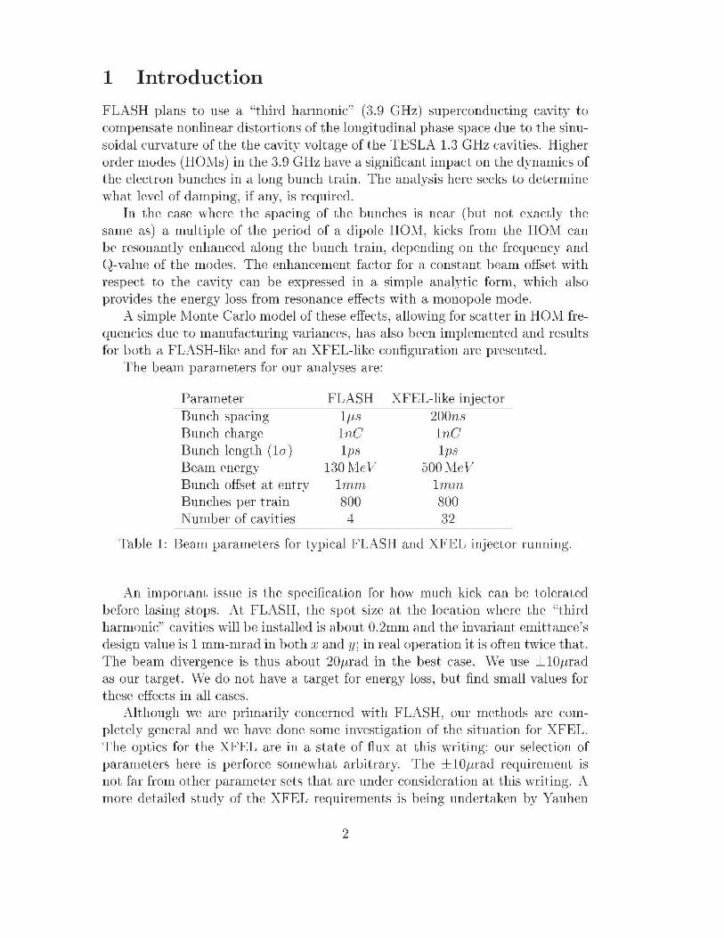
FLASH plans to use a ':third harmonid' (3.9 GHz) superconducting cavity to compensate nonlinear distortions of the longitudinal phase space due to the sinu­soidal curvature of the the cavity voltage of the TESLA 1.3 GHz cavities. Higher order modes (HO.ivls) in the 3.9 GHz have a significant impact on the dynamics of the electron bunches in a long bunch train. The analysis here seeks to determine \vhat level of damping, if any, is required.

In the case where the spacing of the bunches is near (but not exactly the same as) a multiple of the period of a dipole HO~'vI, kicks from the HOJ\;1 can be resonantly enhanced along the bunch train, depending on the frequency and Q-value of the modes. The enhancement factor for a constant beam offset ·with respect to the cavity can be expressed in a. simple analytic form, ·which also provides the energy loss from resonance effects ·with a. monopole mode.

A simple .ivionte Carlo model of these effects, allowing for scatter in HO}I fre­quencies due to manufacturing variances, has also been implemented and results for both a FLASH-like and for an XFEL-likc configuration arc presented.

The beam parameters for our analyses are:

Parameter 13unch spacing Bunch charge Bunch length (lrr) Beam energy Bunch offset at entry Bunches per train Number of cavities

FLASH lps lnC lps

130 ~vic \ 7

lmn1 800

4

XFEL-like injector 200ns lnC lps

500 }IcV lrnrn

800 32

Table 1: Beam parameters for typical FLASH and XFEL injector running.

An important issue is the specification for how much kick can be tolerated before lasing stops. At FLASH, the spot size at the location \vhere the ':third harmonicn cavities will be installed is about 0.2mm and the invariant emittance's design value is 1 mm-mrad in both :r: and y; in real operation it is often twice that. The beam divergence is thus a.bout 20prad in the best case. \Ve use ±lOprad as our target. \Ve do not have a target for energy loss, but find small values for these effects in all cases.

Although we arc primarily concerned with FLASH, our methods arc com­pletely general and we have done some investigation of the situation for XFEL. The optics for the XFEL are in a state of flux at this ·writing; our selection of parameters here is perforce somewhat arbitrary. The ±l01Lrad requirement is not far from other parameter sets that are under consideration at this vaiting. A more detailed study of the XFEL requirements is being undertaken by Yauhen

2

Kot and Thorsten Limberg. \Ve do not here allmv for betatron phase advance bet\veen the cavities, and this effect will be larger at the XFEL than at FLASH.

2 Wakefield due to HOMs

The purpose of this section is to define the parameters that are important for the long range wake field calculation. Our development follows reference [1] closely.

2.1 Modes in a cavity

2.1.1 The electric and magnetic fields

Consider a monopole (m = 0) or dipole mode (m = 1) mode with the frequency f = w / (2 7r) in a cavity ·with cylindrical symmetry. One obtains in complex notation for the electric and magnetic field:

E (r, c,!J, z, t) = ( E~~) (r, z) cos(m ¢) er

+ E~m) (r, z ) sin(rn (/J) e<P

+ E~m\r,z) cos(m¢) ez ) exp(-iwt)

( B!::_) (r, z) sin(n1, ~D) er

+ -8..t\r, z) cos(rn (jJ) e<P

+ Blm)(r, z ) sin('rr1q)) ez ) exp(-iwt).

2.1.2 The loss parameter and R/Q

(1)

The interaction of the beam 'vith a cavity mode is characterized bv the loss parameter k11m) (r) or by the quantity R/ q"' [2]. These parameters car~, be deter­minated from the numerically calculated fields using the l'v1AFIA post-processor [3, 4]. The longitudinal voltage for a given mode at a fixed radius r is defined as

L ·-i~ I( m) (r) = r dz E,~m) (r, z) exp(-i w z/c),

.lo

\vhile the total stored energy is given by:

3

(2)

(3)

From the voltage and stored energy the loss parameter and fl/ Q can be cal­culated:

k(m) (r) IVl1(m) (r) 12

4U(m)

(4)

R(m) 1 2 k(ml(r)

Q r2m w

For monopole modes the superscript (0) is usually omitted R/Q = fl(o) /Q. Al­though our definitions include a radial dependence in the loss parameter; R(m) /Q is independent of the radius r since it can be shmvn (see [2; 5]) that v(m) (r) f"V rm and therefore kCml(r) rv r 2 m.

2.1.3 The geometry parameter G 1 and the Q-value

The pmver I'.~ur dissipated into the cavity wall due to the surface resistivity R.rn.r can be calculated from the tangential magnetic field:

1 I 2 P.rnr = 2 flsur , dA IHsurl · (5)

For a superconducting cavity the surface resistance is the sum of the BCS (Bardeen, Cooper; Schrieffer) resistance RRcs, which depends on the frequency and the temperature, and a residual resistivity R 0 . The BCS resistance RRcs scales ·with the square of the frequency .f and exponentially ·with the temperature T:

. J2 RJJcs(.f; T) oc T exp(-1.76 TjT). (6)

The less-·well understood residual resistance R-0 adds directly to RJJcS' but remains in the limit T ---+ 0.

The total damping of a cavity mode is not only determined by the surface losses but also by coupling to external waveguides (HOIVI-dampers). Therefore one has to distinguish the Q-value Q0 which is defined above and the external Q-value Qcxl \vhich characterizes the coupling to external vvaveguides. Typically,

Qo >> Qc:z:l· The geometry parameter G 1 [6] is defined as:

(7)

G 1 is a purely geometric quantity that is independent of the cavity material; it depends only on the mode and the shape of the cavity that creates that mode.

4

r

C'

·~

Figure 1: A point charge q1 traversing a cavity with an offset r 1 followed by a test charge q2 with offset r 2 •

2.2 Wakefields

2.2.1 Wake potential

Consider the situation shown in Figure 1. A test charge q2 folhws a point charge q 1 at a distant s. The distant s is positive in the direction opposite to the motion of the point charge q 1• Both charges are relativistic ('o ~ c). The Lorentz force on the test charge due to the fields generated by the point charge q1 is

dp F = - = q2 ( E + c ez x B).

dt The wake potential of the point charge q1 is defined as:

(8)

(9)

The \Vake potential is the integrated Lorentz force on a. test charge. Causality requires W (s) = 0 for s < 0.

The longitudinal and transverse components of the ·wake potential a.re con­nected by the Panofsky-\Venzel theorem [7]

(10)

Integration of the transverse gradient (applied to the transverse coordinates of the test charge) of the longitudinal ·wake potential yields the transverse vvake potential.

2.2.2 Multipole expansion of the wake potential

If the structure traversed by the bunch is cylindrically symmetric then a multi pole expansion can be used to describe the wake potential. The location of the bunch train in the ( r, </J) plane will break the symmetry and determine the a11imuthal orientation of the m > 0 modes. Consider a.gain the situation shown in Figure 1.

5

Assume that the point charge q1 traverses the cavity at position (r1, (f?i), while the test charge follows at position (r2, (f'.)2). The longitudinal \vake potential may be expanded in multipoles:

00

H]1(r1,r2,(f'.)1,(f'.)2,s) = L ,.,rn,,.2m n·1im)(s) cosrn((f'.)2 -(f'.)1)- (11) m.=0

The functions Hl[m) ( s) are the longitudinal m-pole \Vake potentials. There is no a-priori relation between the vvake potentials of different azimuthal order m.

The transverse 'vake potential can be calculated using the Panofsky-\Vcnzcl theorem, and the transverse Jn-pole wake potentials arc defined as:

l F(m) ( -,) - 1·8 d -/ l,rr(m) (-.I) ·r_L 8 -- 8 '"II 8 '

--oo (12)

for rn > 0. There is no transverse monopole wake potential. The dipole wake potential docs not depend on the position of the test charge q2 • The kick on the test charge is linear in the offset of the point charge q1 .

2.2.3 Wakefields due to HOMs

It is possible to write the m-polc wake potentials H·i[m) (s) as a sum over all modes:

n1im)(s) = - L Wn(RQ(m)) cos(wns/c) exp(-1/Tn s/c) n n

(13)

(R(m)) :l(m) -, - _· - .' - ' , - ~ n 1- (.s) - c L Q _ sm(wn s/c) exp( 1/ 'n s/c).

n n

where Wn are the frequencies of the m-pole modes. A damping term has been included with the damping time Tn for mode n. As Q0 > > Oe:rt, the damping time of the voltage is very nearly

(14)

3 Effects of long range wakefields on a bunch train

3 .1 Energy deviations and kicks on the bunches

The long range \vakes due to HOivis can cause energy deviations and kicks on the bunches. A bunch train of JV bunches is shovm in Figure 2; the notation for the offsets with respect to the reference axis of the accelerator is .Ti and Yi and the

6

z

y

x

s

v = c e z

x

yx

y

j

jn

n

An energy deviation of 196 eV corresponds to an impedance (R/Q) of 10 0 and

a. loss parameter of k~o) = 0.188 V /pC. The factor 1/2 is a. consequence of the fundamental theorem of beam loading.

Kmv consider the transverse long range ·wakefields. The kick on bunch n due to the dipole vvake field is:

(Jn = (17)

where E11 is the energy of bunch. The kick on bunch n due to one dipole mode with revolution frequency ~·1 and damping constant T 1 is:

where the kick amplitude en on bunch n is defined as

R (l) (}~ _ C qh11.nch , · , . n- E . c--ru;

bea.m Q (19)

with respect to an arbitrary reference offset r 0 •

3.2 One dipole mode and a bunch train with constant offset

It is instructive to consider the simplified situation of a bunch with a constant offset ·with respect to the :'third harmonic'' cavity. This corresponds to an injec­tion error or an misalignment of the cavity. Since the long range dipole \Vakefield is a linear superposition of HOJVIs it is sufficient to consider only one mode at a time in all analytical formulas.

1viodcs from the first 3 dipole pa.ssbands with the highest values for R (1l /C2 arc summarized in table 2; taken from reference [8], !_llong with high R(m) /Q modes of other azimuthal number. The kick amplitude (} for the dipole modes has been calculated according to Equation 19 assuming that all bunches have the same energy of 130 .MeV: bunch charge of 1 nC and reference offset of 1 mm.

Furthermore it is now assumed that the bunch to bunch distance D.t is con-st ant:

6-8 1 D..t = -. = nfb -:

C !Jv (20)

where .ftu = 3.9 GHz is the frequency of the fundamental mode and nfb is the number of free buckets bet\veen bunches. The follmving bunch distances have to be considered for the operation of the injector linear accelerator:

8

.f / GHz m R(m) /Q / G1/ k (m) /r~2m) / 1i / prad n/cm(2m) n V /(pC crrl1m ))

7.506 0 23.3 475.5 0.55 4.834 1 50.7 277.3 0.77 1.22 5.443 1 20.9 426.2 0.36 0.50 7.669 1 29.5 470.7 0.71 0.71 9.133 2 11.2 402.9 0.32

Table 2: RF-parameters and kick amplitude of modes with high fl(m) /Q. For the dipole modes (rn = 1), the kick amplitude has been calculated for an beam energy of 130 :\foV, a bunch charge of 1 nC and an reference offset (ro) of 1 mm.

6t / ns 1/ 6t / JVIHz nfu 200 5.0 780

1000 1.0 3900 2000 0.5 7800

10000 0.1 39000

Table 3: Typical bunch to hunch distance for the operation of injector linear accelerator

The bunch distance can he translated into a phase distance r5 between bunches:

r5 ;\t 2 fi = w-, Ll. = 11-.- n fb, f Ju

(21)

where w1 = 27f .f1 is the frequency of the considered dipole mode. A small change in the dipole frequency due to fabrication tolerances '.Vill cause

a large change in the bunch to bunch phase since the number of free buckets is relatively large. One obtains for a bunch distance of 1/ 6t = DIHz:

1 66 = 211-f . nfh 6f1

. Ju

0.360 6f, kHz

(22)

(23)

A change of 10° in the bunch to bunch phase after n f b = 3900 free buckets corresponds to a frequency shift of about 20 kHz, ·which is much smaller than the expected variation due to manufacturing variations.

A bunch to bunch damping constant for the kick voltage is defined as:

w, . . f, 1 d = -)-6t = 211-f nfb -----r)1

2 (t:' 1 . Ju 2 lti (24)

where Q1 is the Q-value of the dipole mode, \vhich is usually dominated by the external Q-value of the HCnI damper. \Ve give most of our expressions both

9

1e-05

0.0001

0.001

0.01

0.1

1

10

100

1000 10000 100000 1e+06 1e+07 1e+08 1e+09

d

Q-value

Damping constant d for 1 MHz bunch spacing

f = 4.8 GHzf = 5.4 GHzf = 7.6 GHz

d = 0.50d = 0.15

due to one dipole mode are:

·where

_ ( 1 n-1 ) 0.En = E 2 + 2= cos(6 (n - j)) exp(-d (n - j)) ,

J=I

n-1

if L:sin((5(n-j)) exp(-d(n-J.)), j=l

( ! ) - R 2 E = -eqw1Qro , and

- C q R ( I) B= ----r0 .

E 0 /c Q

(25)

(26)

(27)

r 0 is a reference offset. The above expression (25) and (26) can be rewritten as

0.En ff(}+Re(Sn)),

(28)

with a sequence of complex sums Sn, defined as

n-1 n-1

Sn= L exp ((n - j) D) = L exp (.j D). (29) j=l j=l

The complex damping constant D is defined as D = i 6 - d. The sequence S11

may be calculated via a recurrence relation:

0

(Sn+ 1) exp(D),

or via an explicit expression for the sum of a geometric series:

S1)' = 1 - exp((n - 1) D) 1 ------- -----+ for n -+ oo.

exp(-D) - 1 exp(-D) - 1'

Furthermore let Rn be defined as:

exp((n - 1) D) Rn= ( ) exp -D -1

so that Sn = lim Sn - Rn.

n--+oc

The explicit expressions Re (Rn) and Im (Rn) are

e-nd (cos(n6) - e-d cos((n - 1) o)) Re (Rn) =

1 - 2 e-d cos(o) + e-2d

Im (Rn) e-nd (sin(no) - e-d sin((n - 1) o))

1 - 2 e-d cos(c5) + e-2 11

11

(30)

(31)

(32)

(33)

(34)

-4

-3

-2

-1

0

1

2

3

4

5

6

7

-180 -150 -120 -90 -60 -30 0 30 60 90 120 150 180

!

Functions FR,n and FI,n

FR,nFI,n

is much larger than ±21r. Consequently, it is valuable to calculate the average and therms value of FR,n(O; d) and Fr,n(O; d) over the range -71 ~ c5 ~ 71. \Ve are also interested in the absolute kick amplitude which is measured as the average of IF1 ,n ( 6, d) I· These a.re:

1 /" - - 1 -:--2

d() FR, n ( (); d) = -:-2 . 'if . -'ii .

(37)

1 j'" -, d6 Fi,n(6, d) = O 2 7f -r.

(38)

1 l7r - ( - ) - d() F1,n (), d 7f . 0 .

1 n-11- (-l)k - L exp(-kd) 7f k= l k

1 (exp(-nd) d ) - . H (n., d) + ln( coth( ;-- ) ) , 7r n 2

(39)

where the function H(n 1 d) is defined in terms of the hypergeometric function 2F 1

[9] as:

H(n,d) = (-lt 2F1(1,n;n+l;-exp(-d))- 2F1 (1,n;n+l;exp(-d)) (40)

Furthermore one obtains for the IlJvIS-values

R~vIS(FR,n) =

RJvIS(F1,n)

-1- r d8 FR,n((5, d)2

2 7f ./_,.

1 exp(-nd) sinh((n - l)d) - + ----------4 2 sinh(d)

1 + a2 - 2 a2n

4 (1 - a2 )

cxp(-nd) sinh((n - l)d) 2 sinh(d)

1 a2 - a2n

2 (1 - a 2 ) ·

For small ( « r1.) values of d \Ve have:

0=-1 Rl\!IS(F1,n) ~ y ~ ford---+ 0.

13

( 41)

( 42)

( 43)

0.1

1

10

100

1 10 100 1000 10000

bunch number n-1

RMS(FI,n(d))

d=0.1d=0.01

d=0.001d=0.0001

d=0.00001

d 0.1 0.01 0.001 0.0001 0.00001 n 13 118 1165 11641 116397

Table 5: Bunch number n for \vhieh the ratio of RTvIS values of the function Fr,n and FI is equal or larger than r = 0.95.

3.4 The asymptotic functions FR and F1

For nearly all cases of interest, the functions Fu,n ( b, d) and F1 ,n ( 8) d) reach their large-n asymptotic limits Fu( 8, d) and F1 ( 8) d) after only a small fraction of the hunch train has gone through the cavities. The expressions in this section arc then useful.

FI(6, d)

1 . - + lnn Ile (Sn) 2 n-+x

1 - e-'2d

2 (1 - 2 e-d cos(b) + e-2 d)

sinh( d) 2 (cosh(d) - cos(o))

1- a2

2 (1 - 2a cos( 6) + a2)

lim Im (Sn) n-+x

e-d sin(8) 1 - 2 e-d cos(8) + e-2 d

sin(b)

2 (cosh(d) - eos(8)) ·

a sin ( 6) (1 - 2acos(8) + a2)

( 46)

( 47)

A plot of these functions is shown in Figure 6 for a damping constant d = 0.15. Fundamentally, we are exciting a simple harmonic oscillator \vith a train of

6-function pulses; and FR( 6, d) is proportional to the response of the oscillator. It shows a characteristic resonance bell-shape, with the peak at the condition \Vhere the 8 pulses arrive at any sub-harmonic of the oscillator. The functions Fll(b, d) and F1 ( o, d) are asymptotic amplification factors along the bunch train; there is no hunch-to-bunch amplification of the energy deviation flEn or kick (;Jn if these functions arc smaller than one.

The average and the nns values of FR(o,d) and Fr(o,d) for -K-<::: o-<::: 7r are:

(Fu) 1 ;·7r 1 -. do Fll(b, d) = -2 7r -)T 2

( 48)

(Fr) 1 l7r - (" ) -. - d() Fr o, d = 0 2 7f . -7r ( 49)

15

-4

-3

-2

-1

0

1

2

3

4

5

6

7

-180 -150 -120 -90 -60 -30 0 30 60 90 120 150 180

!

Functions FR and FI

FRFI

1

10

100

1000

1e-05 0.0001 0.001 0.01 0.1

d

RMS(FI(d))

0

1

2

3

4

5

6

0 30 60 90 120 150 180

!

Function FI

d = 0.50d = 0.15d = 0.10d = 0.00

0.1

1

10

100

1000

0 0.1 0.2 0.3 0.4 0.5 0.6 0.7 0.8 0.9 1

d

Maximum and RMS of FI

Max(FI) RMS(FI) Max = 1.0Max = 3.3

The probability P that Fr( o, d) is larger than one is therefore approximately

1 Pr1 >1 ~ - arccos(3/5) ~ 0.3.

1r (63)

The amplification of the kick due to one H01I is expected to be smaller than one in about 70 % of the cavities of all possible random phases. Since several modes have to be considered the overall result will be different from this optimistic one-mode scenario (sec the discussion in section 3.6).

The probability that the function Fr(O; d) is larger than a constant A can be estimated from the proability that the function fr(o) is larger than A. In general we have:

(64)

For many practical cases it is Pp1 >,1 ~ PI1 > ,1 if the constant A is smaller than _\fax [Fr].

3. 5 The RMS kick over a bunch train due to one di pole mode

In the previous section 'NC have discussed the asymptotic kick on the bunch train. The average and R\IS values of the asymptotic function FR ( c5, d) and F1 ( c5, d) have been calculated for the phase o. l\mv vve drop the asymptotic limit, and average the kick (Jn for finite bunch munber n. \Ve give the Il.\IS kick over the bunch train as \vell. \Ve retain the full form of the kick

(65)

where F1 and Rn are defined as in Equations 47 and 32. The average and the R.\'18 of the kic~s over IV bunches in the train, normalized \vith respect to the kick amplitude (} arc

(e) ;e 1 N F1 - - '°"" Im ( R ) V ~ n

• n = l

R.\rn( e) ;e 1 '" ( 1 .\ ) 2

;V r~ (Im (Rn)) 2 - JY ?; Im (Rn)

The analytic expression for the sums are:

1 N --;! L Im (Rn) J\ n = I

- (N+2)d e 1

2N 1 + e- 2d - 2 e-d cos( 6)

. ( ) 1

. (') · (cNd(c2

d - 1) sin(6)+ cosh d - cos o

20

(66)

(67)

(68)

~T t (Im (Rn))2 ~ n=l

2edsin(Nc5) - e2dsin((2V + l)c5) - sin((N - l)o))

1

N (l + e-2d - 2e-d cos(r5)) 2

( ( _) cosh ( d) . ( _ ) ) - cos 6 + . ( ) srnh .N d +

srnh d

e-2(1V+:>) d 1

2N 1 + e-2d - 2 e-d cos( c5) 2

1

1 + e-~d - 2 e-2d cos(2 c5)

( 2 e(2 N+i) d(e2d - 1) cos(6)+

e2Nd(e

4d - 1) cos(2c5) - cos(2 (iV -1) c5) +

e~ d cos(2 (2V + 1) 6) + 2ed cos((2N - 1) 6) -

2e3d cos((2N + 1) c5))

(69)

\Vhile the general analytic expression for the average and the nns kick over a bunch train of N bunches a.re rather complicated the expressions in the limit of no damping at all (d -t 0) are much simpler:

lim (FJ) /0 d-tO

(70)

---.-- - Sm 0 1 (sin(Nb) . -) 2 (cos(b) - 1) N

lim RMS ( FJ) / {j d-tO

(71)

1 2 (1 _ . _ ., (,\)) _ 2 sin(N8) 2 + sin(2 1V 8) tan(J) 2

_ COS u N~ N

2 (1 - cos(c5)) 2

Furthermore one may look for the limit of the functions Ave0(N, b) and Rms0(N, 8) for long bunch trains ( N -t x). Provided the limit is ta.ken \vi th constant b, so that.JN -t oo,

lim Ave0(N, 8) lV-tx

1 8 - cot(-) 2 2

(72)

lim F1 (b, d) d-tO

21

0

5

10

15

20

25

30

35

40

0 5 10 15 20 25 30 35 40 45!

Average kick, 100 Bunches

AveFI, d = 0

3.6.1 An estimate based on the asymptotic RMS kick

An estimate using an Rl'vIS approach and including a sum square combination of the different modes in the cavity is:

(74)

If the damping constants of all modes are identical one obtains for 4 cavities:

(}RAIS RMS(F1)(d) ~ = RJvIS(F1 )(d) · 2.991,urad

(75)

(76)

The value 2.99lp,rad is based on the values in table 2. Equation (76) can be used as a criteria to determine the damping constant. d. If 'NC demand that. the combined R~v1S kick should not exceed half of the single bunch divergence:

2.991 /ffad · R\1S(Fr )(d) < 10 wad: (77)

one obtains for the required damping constant drmslO:

drmslO = 0.0219 . (78)

The corresponding Q-values of the modes are listed in Table 6 and the function Fr ( r5, drmsl 0 ) is plotted in Figure 11 for 0 ~ r5 ~ 7r. The IU\-1S and maximum of

f /GHz Qext

(1/ !:::.t = 1 l'v!Hz) 4.834 6.9 x 105

5.443 7.7 x 105

7.669 1.1 x 106

CJe.rt

(1/ !:::.t = 5 1vIHz) 1.4 x 105

1.5 x 105

2.1 x 105

Table 6: Q-va.lues of three modes for a damping eonstant d = 0.0219 and bunch­to-bunch distances of 1000 ns and 200 ns.

the function Fr(r5: d) for the damping constant dnnslO = 0.0219 are:

RivIS(Fr) (dnnsrn) = 3.33, IVIax [Fr] (dnnsrn) = 22.9 . (79)

So in the vmrst but very unlikely case the total kick can be:

;~

lVIax [F1] (drms10) · 4 L {jk (80) k=l

1vlax[F1] (drms10) · 9.71/trad = 222.4,urad.

23

0

5

10

15

20

25

0 30 60 90 120 150 180

!

Function FI

FIRMS(FI)

The R\IS value of the maximum possible kicks is smaller than l011rad if d =

dmvrs = 0.15, since (85)

The corresponding Q-va.lues are summarized in Table 7. The RNIS of the function

f /GHz Qext (1/ 6.t = 1 TvlHz)

4.834 1.0 x 105

5.443 1.14 x 10·5

7.669 1.6 x 105

Qe.r,t (1/ 6.t = 5 IVIHz)

2.0 x 101

2.3 x 101

3.2 x 101

Table 7: Q-values of three modes for a damping constant d = 0.15 and bunch-to­bunch distances of 1000 ns and 200 ns.

F1 ( J, d) is 1.2 and therefore

HRlvis Rl\IS(Fr)(dR11Is) · 2.99111,rad

3.59 prad ,

81or Max [Fr] (dmvrs) · 9.71 prad

32.2 prad .

(86)

(87)

Even in the worst case the total kick will only be a factor 1.5 larger than the single beam divergence of 20 prad.

One of the most strict alternatives is to constrain the worst case of the total kick to 10 prad:

3

Btot < :'viax [Fr] (d) · 4 L Ok (88) k = l

:'vfax [F1] ( d) · 9. 71 prad

< 10 prad

If the damping constant d is larger dmax = 0.47 we obtain

Max [F1] (d) :::; 1.03 , (89)

and the constrain Btot :::; 10 prad is met. The eorresponding Q-va.lues arc listed in Tab. 8. For this very strict eonstraint \VC have:

eRTlfS = R:VIS(Fr) (dmax) . 2.991 ttrad = 1.69 µ.rad . (90)

25

f /GHz

4.834 5.443 7.669

Qext

(1/ !:1t = 1 l\1Hz) 3.2 x 101

3.6 x 104

5.1 x 104

CJe.rt

(1/ !:1t = ;) MHz) 6.5 x 10a 7.3 x 103

1.0 x 104

Table 8: Q-values of three modes for a damping constant d = 0.47 and bunch-to­bunch distances of 1000 ns and 200 ns.

4 Monte Carlo Analysis

The problem has also been attacked eomputationa.lly with a simple 1-fontc Carlo calculation. A worst-case analysis for a single cavity, and typical-case analyses for both FLASH and XFEL configurations have been made. The analysis provides, with certain assumptions, CJe~:t requirements.

The analysis does alluw for the scatter of HO}I frequencies that ·will no doubt result from variations \vithin tolerances of the cavity dimensions and shapes that a.re pa.rt of the ma.nufaeturing tolerances. The analysis docs not a.llmv for the possibility that if HOM dampers fail utterly, fields may remain in the cavity for the relatively long time between bunch trains. Perhaps most importantly, there will be some active-feedback beam steering system that should ameliorate beam deflection effects and this remains still to be studied.

4.1 Method

The analysis is best explained by describing the objects from \vhich it is made. A mode is basically a frequency, an R~; l value, an azimuthal quantum number and a decay time. A cavity is a collection of modes and the corresponding vrnkefield functions H'll and HlJ_. A beamline is a set of cavities, \Vith the kicks and energy losses from each of the cavities summed.

A tcdmical note: the algorithm dircetly implements Equation 13 and for the bunch train lengths under consideration here, that requires taking the sin(fJ) and cos(fJ) for very large values of fJ indeed. Care has been taken to verify the numeric precision of these functions in this specific implementation of the algorithm.

All the modes listed in Table 2 are included in the simulation, although the quadrupole mode has a negligible effect. The effect of the monopole mode on the beam energy is computed, although we have concentrated on the transverse dynamics. A sixth entry exists in the code for the 3.9 GHz operating mode, but it is switched off and is not used.

26

4.2 Single cavity worst-case analysis

The \vorst-ca.sc is where a. cavity has a HOl\I with a peak in Fr that is directly on beam resonance and the cxtcrna.l dampers have failed so that damping is provided by the intrinsic power dissipation of the I\b surface a.lone. In this case, the asymptotic limit is not reached; the bunch train is not long relative to the wakefield time scale. The surface resistance is modeled from 3.9 GH:;r, \vith an R 8 cs of 20n0 scaled with the square of the frequency ratio, plus the residual resistance, R0 , of 20n0. The CJ-value is then obtained by dividing C1 of the mode by this resistance.

The monopole mode ·will, with over 800 bunches in the FLASH configura­tion, take about 800 ke \/ out of the last bunch in the train. The maximum of Fr corresponds to about 468 Hz from the exact on-resonance condition for all of the dipole modes 2

• The deflection from the dipole mode of highest R~ml in this case is shown in Figure 12; the other modes have the same shape but \vith the vertical scale proportional to R~;') . Figure 13 shows the crabbing angle, defined as the deflection angle (in the lab frame) at the laz bunch head minus the de­flecting angle at the bunch center. This is computed by changing, in effect, the trailing distance of the witness by one bunch-length, and taking the difference in displacement from the centroid displacement.

\Ve do not have a clear understanding as to how this can effect the lasing process, but note that the angles involved are typically smaller than the deflecting angles. The energy loss in this dipole mode at this pseudo-resonance condition is only 5ke1,.. .

It. is dear that even a single cavity hitting the worst-case will cause lasing to stop.

4.3 Typical-case analysis, FLASH beamline

In the typical-case analysis we use the ~fontc Carlo method to examine the prob­ability distribution for hcamlinc performance.

A virtual beamline is constructed of 4 cavities. The frequencies of the modes are shifted from the nominal simulation results of Table 2 by drawing on a uniform random distribution. The ·width of the distribution spans the full range of 6, corresponding to a frequency shift of -0.5 1vIHz to +0.5 IVIHz in the FLASH case, and l/5th that for the XFEL injector. \Vhile \Ve do not have enough cavities to really check, this is thought to be about the scale on which the scatter will actually be.

Simulated results such as in Figures 12 and 13, along ·with the corresponding energy loss plot are recorded. Then a ne\v beamline, constructed with new calls to

21n the long, bunch train limit, the maximum would occur at 6.f = f /2Q. However, without damping, 800 bunches is not near the long bunch train limit. Additionally, there arc large-~ oscillation effects, as described in section 3.4.

27

Bunch100 200 300 400 500 600 700 800

mrad

-0.7

-0.6

-0.5

-0.4

-0.3

-0.2

-0.1

-0

Bunch100 200 300 400 500 600 700 800

mrad

0

0.002

0.004

0.006

0.008

0.01

0.012

the pscudo-ra11dott1 number gm1crator is c:.reated and again, variation of deflection, nabhiug, aud t>11ergy loss wit.h respe<:t. t.o lrn11d1 1111mher i:< det.er111i11ed. The process is repeat.t><l .)000 or i11 some <:n.ses, I 0000 t.imes. At. en.ch bunch r111ml>er, we havP. an a.verage a.nd a.u R.:VIS. ovP.r 1.hose bea.mlines. nf drdlec1.i.-111, era.hbiug, 1:1.ml energy loss.

The 1:1.vernge drfieetion over an ensemble i~ e1:1.sily seen 1.0 be :tern, as <lelleeUon to the left i~ just as likely a!> deflection to the right. The average energy Joss is alw 7.cro: the sin of F:quation Ub i' replaced by the co' of Fquation l:fa. l'he width:; of the distributious of deflection a11glc, crabbing angle and energy Josi; describe ll.t t.he 10' lewl what. kiud of performa11<·t> one rn.n expt>c:t wht>11 the rmu:hine is n.c:t mi.I ly turned 011.

Cle;irly, a design 1.hal will keep dPllecl.ion down 1.0 0111· ±Hlf1.r<1.d goa.l at. 1.he G8.27'7< (la) confidence level is risky; we need the RMS l.o be well below Uie goal. llow far below i~ a difficult deci~ion involving overall program risk. .\101.with­standing, a statistical analy~is is able to provide us with a good !>ense of what levels of external damping we need to have.

Ap;;,iin, we do not obt<iin an <itccpt;,tblc result m1 jui;t cavity self~damping alone. Tf t.he HOM desig11 fa.ib n.c:ross the honnl, deflections of "' ±i:i011.rad nppt>a.r a.t the I rT level hy the eud of 1w 800 lmud1 trn.i11 in t.he 4 <:nvity. 5 rnode FLASH model, as ;;!iown iu Figure H. :>Jext., we del.enniue how far we ~m11;;1. lower lte:r.t

to sl.abili:te t.lic. bram.

Bunch

Figure 1 'l: The onc-5igma delleelion profile as a func:Uon of bunch number, avcr­ari;ed over ensemble.\ of C.000 virtual I·"! .!\SH beam liner,; without external damper!:'.

For tht> 7.i:iOo \:!Hz HIOJlOpolt> mode. lmwriug qocr.t to a bit. helow Ix I 07 <:a.lJSt'~ the R:VfS of 0..F. t.o flat.ten out n.t ln.rge bunch m1mbers to about :.n kf:F.

29

For the dipole modes, there is some allocation of the ±lOprad target into the three modes; we have to also allocate fractions of the deflection budget to the different deflecting modes. If \Ve require that the R:VIS deflection flattens out to a level \Vhere ±lOprad corresponds to 3a of the total deflection, and then allocate the deflection budget evenly among our three large dipole modes, then

each mode must contribute 10/trad/ (3/(3)) = l.9pra.d in the asymptotic limit for the 4 cavities, as the contributions from the included modes are added in quadrature.

The IVIontc Carlo ca.leulation differs from the analytic form of section 3.6.1 in that.

1. In the l\IC met.hod, the asymptotic limit. is not. assumed. It ·will in most cases he justified because the damping is strong.

2. In the .\IC method, angles are summed over modes and cavities, and then an RJl/IS is ta.ken; in the analytic form, the sequence of these tvvo operations is inverted.

3. In the analytic form, the damping constants of all the modes arc forced to be equal; in the l'l/IC method, the deflection in the long-lmnchtra.in limit. arc ta.ken to be equal.

4. Equation 77 sets lOprad to 1 times the R.\!JS deflect.ion; section 3.6.2 dis­cusses alternate, tight.er constraints. The 1.-IC met.hod uses a 3o- constraint..

The l\font.c Carlo results can be reproduced \vith analytically. \·Vit.h the re­quired values of C2e:r;t, the asymp0t.ic form of Equation 53 permits direct. solution for Qe.rt using the definition of H and d. These relations lead to C2ext for the 3 modes of 3.7 x 10~, 2.:) x 10·5 and 1.7 x 105 , or about 70-80% of the IvIC values.

The Qexl values that produce deflections of the specified level in the Monte Carlo, found basically by trial and error, are shO"wn in Table 9, along ·with the results of section 3.6.1 ·when a 3a constraint is used, the results of Phillipe Piot's (unpublished) calculation and the recent measurements from prototypes [10]. The system is ·well damped in the simulation, as shown in Figure 15.

4.4 Typical-case analysis, XFEL injector beamline

The typical-case analysis for our canonical XFEL configuration shmvs, as ex­pected, that the RMS deflection due to HO.\Is varies inversely as the beam energy and approximately as the square root of the number of cavities. This makes the deflection about 2/3 of what it ·would be in FLASH at. the same bunch spacing.

Moving the bunch frequency up to 5 :VIH z changes the relative contribution of the dipole modes by changing d and thereby increases the accumulated deflec­tions. \\There the asymptotic IUvIS values of the deflections, scaled to 24 cavities

30

Bunch100 200 300 400 500 600 700 800

mrad

-0.003

-0.002

-0.001

0

0.001

0.002

0.003

Frequency Azimuthal (GHz) rmmber 7.506 () 4.834 1 5.443 1 7.668 1

Qe.J:t

.\IC method 3o- Analytic 1.0 x 107

2.4 x 104

1.3 x 105

1.0 x 10s

1.8 x 104

2.0 x 104

2.8 x 104

Table Hl: Cdext requirements from this l\'Ionte Carlo study and the analytic forms of 3.6 .1 \vhen calculated for a 3o- constraint. The XFEL beam para.meters are used.

5 Conclusion

\Ve have studied the Qexl requirements for the '~third harmonic" cavities using sets of beam para.meters typical of FLASH and XFEL operation. A key assumption is that lasing \vill cease \Vhen the deflection due to \Vakefields approaches the divergence of the beam at the cavity location. \Ve have ta.ken the divergence to be ±lOprad for both beam para.meter sets. The XFEL optics in the vicinity of the "third harmonic" cavities is not finalized as \Ve write, but the ±lOprad condition is of the correct scale.

The reader need also be aware of the 'program risk' issue: what level of statistical confidence that this ±10/ffad specification be met without component replacement or change of beam parameters is required? Here, \Ve have selected a. 3o- level of confidence. One might choose to argue that the 3o- choice is too conservative. Choosing a la requirement relaxes the damping requirements by a.bout an order of magnitude.

The results arc based basically on three modes of high beam-cavity coupling. Adding in quadrature a number of other modes \Vi th lmver R(1 l / Q has little influence ( rv25%) on the damping required.

Both analytic and l\'Ionte-Ca.rlo based analysis have been done. Both a.llmv for manufacturing defects, but do not allmv for the action of any kind of active beam steering system and a.re quite conservative in that regard.

The results of the two analyses a.re broadly consistent and arc summarized in tables 9 and 10. It is encouraging that the Qe,rt values measured on prototypes a.re better than the required values.

For damping values of Qr;;xr in the 105 range, which are typical for functioning H0Jv1 mode dampers, the deflections reach their asymptotic values after a few lO's of bunches. In this case, our analytic results a.re particularly easy to use, and \Ve summarize them here.

The angular kick on bunch n E {1, 2, 3 ... } due to a single mode of angular frequency w and quality number Q in a. train 'vith bunches ~t seeonds apart is

32

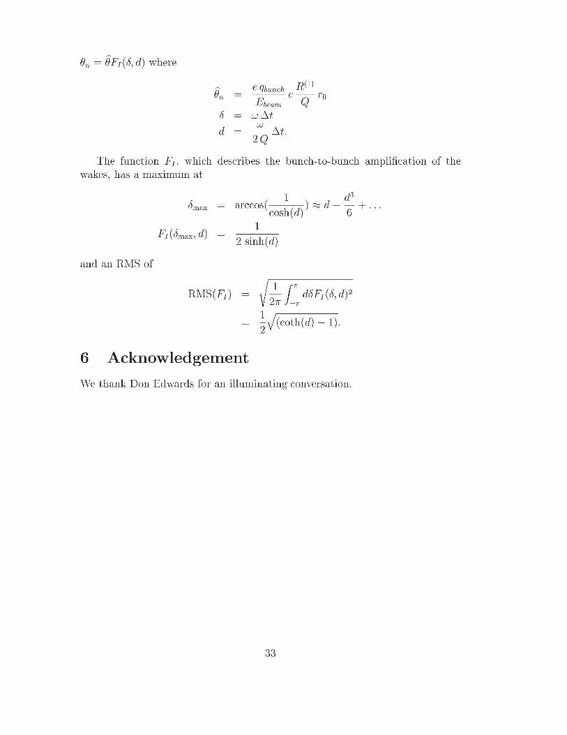
On = iJF,(<5,d) vvhere

r5

d

The function F1 i \vhich describes the bunch-to-bunch amplification of the wakes, has a maximum at

1 d3

arccos( ( ) ) ~ d - - + ... cosh d 6

1

2 sinh(d)

and an RivIS of

R1vIS(F1 )

~y!(coth(d) - 1).

6 Acknowledgement

\Ve thank Don Edwards for an illuminating conversation.

33

References

[1] R. \Vanzenberg: Monopole, D'ipole and Quadrnpole Passband" of the TESLA 9-cell cavity, TESLA 2001-33, Sept. 2001

[2] T. \Veiland, R. \Vanzenberg: Wake fields and impedances, in: Joint CS­CER~ part. acc. school: Hilton Head Island: SC, USA, 7 - 14 l\ov 1990 / Ed. by rvI Dienes: IvI .\fonth and S Turner. - Springer, Berlin, 1992- (Lecture notes in physics ; 400) - pp.39-79

[3] T. \Veiland, On the rmmer·'ical i·wlntion of Ma:J:weWs Eq'aations and Appli­cations in the Field of Accelerator Physics, Part. Acc. 15 (1984): 245-292

[4] MAFIA Release 4 (V4. 021) CST GrnbH, Biidinger Str. 2a, 64289 Darm­stadt, Germany

[;5] T. \Veiland: Comrnent on wake field compntat'ion 'in frrne domain, DESY .\I-83-02: Feb. 1983

[6] P.B. \Vilson High Energy Electrnn L'irwcs: Appl'ication to Storage Ring RF Systems and Linear Coniders, AIP Conference Proceedings 87, American Institute of Physics: ~ew York (1982),p. 450-;563

[7] \V.K.H. Panofsky: \\'.A. \Venzel, Some considerat'ions concerning the trans­verse deflection of charged particles in rad'io-freqnency fields , Rev. Sci. Inst. Vol 27, 11 (1956): 967

[8] \V.F.O. l'vlliller, J. Sekutowicz, R. \Vanzenberg and T. \Veiland: A Des'ign of a 3rd Harmon'ic Cavity for the TTF 2 Photcrinjector, TESLA-FEL 2002-0;), July 2002. T. Khabiboulline, N. Solyak and R. \Vanzenberg, Higher order modes of a 3rd harmonic cavity with an increased end-cnp iris FER.\HLAI3-T1vl-2210, DESY-TESLA-FEL-2003-01: .\fay 2003.

[9] .\'1. Abramowitz: I.A. Stegun, (eds.) Handbook of Mathematical Functions, 9th printing: Dover, Ne>v York 1970

[10] T. Khabiboulline: private communication.

34