c© 2016 James Yifei Yang

DISTRIBUTED CONTENT COLLECTION AND RANK AGGREGATION

BY

JAMES YIFEI YANG

DISSERTATION

Submitted in partial fulfillment of the requirementsfor the degree of Doctor of Philosophy in Electrical and Computer Engineering

in the Graduate College of theUniversity of Illinois at Urbana-Champaign, 2016

Urbana, Illinois

Doctoral Committee:

Professor Bruce Hajek, ChairProfessor Rayadurgam SrikantProfessor Nitin VaidyaAssistant Professor Sewoong OhProfessor Dah Ming Chiu, Chinese University of Hong Kong

ABSTRACT

Despite the substantial literature on recommendation systems, there have

been few studies in distributed settings, where peers provide recommenda-

tions locally. Motivated by word of mouth type of social behavior and the

advantages of sharing resources, we analyze an online distributed recommen-

dation system with joint content collection and rank aggregation. In such a

system, peers contact each other and exchange partial preference information

about items, which, for example, could be videos. Peers use recommendation

strategies to make decisions with limited knowledge and collect items that

are available from the contacted peers. The goal is to maximize the rate at

which peers collect their most preferred items.

Correlated preferences are modeled as rankings generated by a Plackett-

Luce ranking model with Zipf popularity distribution. We establish a per-

formance upper bound and use intuition provided by the bound to design

recommendation strategies with a range of complexity. Among these, the

direct recommendation rule emerges as being particularly simple and yet

effective. The direct recommendation rule is found to be remarkably robust,

working well over a broad range of correlation of preferences, initial video

availability, storage size, peer arrival pattern, and performance metric.

Correlated preferences are modeled as scores generated using an inde-

pendent crossover model. In order to explore performance for large scale

networks, we identify the fluid limit as the number of videos goes to infinity

for a mean field limit derived for the number of peers going to infinity under

a direct recommendation rule. Simulation results show that the limit anal-

ysis accurately predicts performance, not only for the independent crossover

model with scores, but also a model with rankings. The performance of

the direct recommendation rule is shown to be near optimal for large scale

systems.

Correlated preferences are modeled as scores generated using a two-stage

ii

independent crossover model. We propose four recommendation strategies

for heterogeneous preferences. We find that a simple rule, called the nearest

stored preference rule, is as effective as the more complex rules. The perfor-

mance of all the rules is far from a performance upper bound in case the peers

in different clusters are nearly independent. We find through simulation that

the gap can be nearly closed by using either exponential accumulation of

information or neighbor assignments such that most neighbors have similar

preferences.

iii

To my parents Yang Yang and Maizhi Yang

and to my wife Congcong Li,

for their love and support.

iv

ACKNOWLEDGMENTS

Firstly, I would like to express my sincere gratitude to my advisor, Professor

Bruce Hajek, for the continuous support of my Ph.D. study and related

research, and for his patience, motivation, and immense knowledge. His

guidance helped me in all the time of research and writing of this thesis. I

could not have imagined having a better advisor and mentor for my Ph.D.

study.

Besides my advisor, I would like to thank the rest of my thesis committee:

Prof. Rayadurgam Srikant, Prof. Nitin Vaidya, Prof. Sewoong Oh and Prof.

Dah Ming Chiu, for their insightful comments and encouragement, but also

for the hard questions which inspired me to widen my research from various

perspectives.

v

TABLE OF CONTENTS

CHAPTER 1 INTRODUCTION . . . . . . . . . . . . . . . . . . . . 11.1 Motivation . . . . . . . . . . . . . . . . . . . . . . . . . . . . . 21.2 Related Work . . . . . . . . . . . . . . . . . . . . . . . . . . . 21.3 The Basic Peer-to-Peer Framework . . . . . . . . . . . . . . . 41.4 Main Contributions . . . . . . . . . . . . . . . . . . . . . . . . 61.5 Organization . . . . . . . . . . . . . . . . . . . . . . . . . . . 8

CHAPTER 2 RANKING SYSTEM . . . . . . . . . . . . . . . . . . . 92.1 Plackett-Luce with Zipf(α) Model . . . . . . . . . . . . . . . . 92.2 An Upper Bound on System Performance . . . . . . . . . . . . 102.3 Three Recommendation Rules . . . . . . . . . . . . . . . . . . 122.4 Variation: Peers Arriving to Stable System . . . . . . . . . . . 162.5 Performance for Ranking Model . . . . . . . . . . . . . . . . . 172.6 Summary of Results . . . . . . . . . . . . . . . . . . . . . . . 252.7 Derivation of EM Algorithm for Estimating the Master Ranking 26

CHAPTER 3 SCORING SYSTEM AND LARGE SYSTEM SCALING 283.1 Independent Crossover Channel Model . . . . . . . . . . . . . 283.2 An Upper Bound on System Performance . . . . . . . . . . . . 293.3 The Mean Field Limit (N →∞) . . . . . . . . . . . . . . . . 303.4 Fluid Limit of the Mean Field Model (M →∞) . . . . . . . . 343.5 Analysis of the Plackett-Luce Model Using IC Channel Model 363.6 Performance for Scoring Model . . . . . . . . . . . . . . . . . 393.7 Summary of Results . . . . . . . . . . . . . . . . . . . . . . . 423.8 Proofs of Limit Theorems . . . . . . . . . . . . . . . . . . . . 43

CHAPTER 4 THE MULTI-CLUSTER FRAMEWORK . . . . . . . . 514.1 A Generative Cluster Model for Heterogeneous Peers . . . . . 524.2 Upper Bound on System Performance . . . . . . . . . . . . . . 524.3 Clustering: Similarity Measures and Error . . . . . . . . . . . 534.4 Recommendation Rules Based on Stored Partial Preference

Vectors . . . . . . . . . . . . . . . . . . . . . . . . . . . . . . . 594.5 Multi-Cluster Aware Global List Recommendation Rule . . . . 644.6 Performance for Multi-Cluster Scoring Model . . . . . . . . . . 664.7 Summary of Results . . . . . . . . . . . . . . . . . . . . . . . 74

vi

CHAPTER 5 CONCLUSION . . . . . . . . . . . . . . . . . . . . . . 76

REFERENCES . . . . . . . . . . . . . . . . . . . . . . . . . . . . . . . 78

vii

CHAPTER 1

INTRODUCTION

Online social networks have become a big part of our lives. They are espe-

cially helpful in advising people how to make decisions. In particular, there

is a rapidly growing number of objects and growing amount of information

describing the objects. Each person has somewhat different interests and

needs to search for the most relevant objects. Fortunately, in a given class

of objects, people’s preferences are statistically positively correlated, even if

they have some disagreements. This allows for a crowd sourcing effect, where

people can help each other find the most suitable objects. In this thesis, we

take the objects to be videos.

In a traditional video recommendation system, recommendations are pro-

vided in a centralized way. Peers upload preference information to a cen-

tral server and recommendations are computed by the central server. Fur-

thermore, peers only download videos from the server. In contrast, we

examine an online system in which peers are only contacting each other,

with, perhaps, some centralized coordination such as a tracking system.

Peers collect preference information only from their contacted peers and

provide recommendations for each other based on limited knowledge. Then,

peers download videos from their contacted peers. The availability of videos

depends on peers’ past contacts and decisions. Well designed peer-to-peer

systems can require less computational complexity, save server bandwidth

and storage, and resist malicious recommendations made by a server or small

group of peers.

The objective is to have each peer efficiently collect as many personally

preferred videos as possible under constraints on bandwidth, storage, and

information about preferences. A main factor contributing to efficiency is

the choice of recommendation rule that helps peers decide which videos to

collect. Strategies differ in how much preference information is gathered,

stored, and processed.

1

1.1 Motivation

Word of mouth plays an important role in how people make everyday de-

cisions—for example, choosing from candidates applying for a job position,

restaurants in a city, books to read, music to listen to, etc. The setting

of our work is movie videos. Having the peers receive recommendations in

a distributed way could be more helpful than receiving recommendations

from a centralized authority. Good decisions naturally lead to satisfaction,

happiness, and sometimes progress. However, not all choices are equally good

or bad because people have different views. Yet, it is crucial for people to

be efficient in making good decisions because time is a valuable resource.

Since people inherently have similar tastes, we need to find recommendation

strategies to take advantage of this correlation so peers can be efficient in

making good decisions.

1.2 Related Work

A wide variety of recommendation systems have been proposed, mostly

based on a centralized system in which recommendations are generated by

a centralized authority. Some recommendation systems may use matrix

completion techniques offline [1]. Online recommendation systems often use

neighborhood-based collaborative filtering that falls under peer-peer or item-

item paradigms, in which either an item is recommended to similar peers or

similar items are recommended to a peer [2, 3, 4, 5, 6]. Another interesting

aspect of online recommendation systems is cold-start recommendations,

where many peers or many items are added to the system at once. In this

regime, network structures such as social networks are often used [7].

This thesis pertains to an online distributed recommendation system with

content collection and rank aggregation done jointly, starting primarily from

a cold start state. Basic elements of the model were proposed in the pio-

neering work of Cruz [8]. Cruz modeled correlated preferences by assuming

there is a master ranking of videos, and the personal preferences of a peer

are correlated with the master ranking, giving rise to correlated personal

preferences among peers. Cruz studied the content collection problem by

formulating a happiness function to measure how many personally preferred

2

videos each peer has collected. He proposed a solution to the joint rank

aggregation problem based on each peer compiling a lossy aggregate of partial

rankings called the global list maintained by a peer, to be used to assist in

selecting which videos to download.

The choice of rank aggregation method is a major aspect of the system.

There is a large literature on rank aggregation; here we cover the part most

relevant to this thesis. In our work, we assume the observed preferences

are generated from a probabilistic model. There are many probabilistic

models on permutations, some of which are studied in [9] and [10], which fall

into one of two categories: nonparametric models and parametric models.

Jagabathula and Shah [11] studied a nonparametric approach to modeling

distributions over rankings. Most of the parametric models fall into one

of the following three categories: noisy comparison model, distance-based

model, and random utility model. Our work is based on the random utility

model.

The parametric models assume there is an underlying master ranking σ

over m objects. For the noisy comparison model, each peer independently

gives a pairwise comparison which agrees with the master ranking with

probability p > 12

[12]. An example of distance-based model is the Mallows

model, which randomly generates a full ranking σ over m objects from the

master ranking σ∗ with probability proportional to eβd(σ,σ∗), where β is a

fixed spread parameter and d(·, ·) can be any permutation distance such as

the Kemeny distance [12].

In our work, we adopt a special case of random utility model (RUM)

known as the Plackett-Luce (PL) model. Plackett [13] performed analysis on

permutations and Luce [14] formulated theory on individual choice behavior.

The PL model is assumed in many ranking related works. The Bradley-

Terry model [15] is a special case of the Plackett-Luce model obtained when

only pairwise partial rankings are reported. Hunter [16] showed that the

log likelihood function under the PL model is concave and proposed a mi-

norize/maximize (MM) algorithm for rank aggregation under generalized

Bradley-Terry models. He also showed that the algorithm may be prob-

lematic for sparse data due to over fitting. Guiver and Snelson [17] proposed

a Bayesian inference method for the PL model. This method uses divergence

measure and message passing techniques proposed by Minka [18]. In the

work of Cao et al. [19], rank aggregation is done by minimizing a particular

3

metric.

A well known probabilistic model of Thurstone [20] states a law of com-

parative judgment which specifies an unobserved random variable xi for each

object according to a distribution. It is well known that Luce’s choice axiom

is equivalent to the Thurstone model using Gumbel distributed independent

noise, a result attributed to Holman and Marley (see Lemma 6 of [21]).

There are some relations between our work and the theory of opinion

dynamics. The focus of opinion dynamics is on distributed averaging for

consensus problems. Boyd et al. [22], Nedich [23] and many others have

studied the averaging problem under various gossip constraints for different

network graphs. The estimate of the master ranking, in particular the

global list, is similar to opinion dynamics because the global list acts as

a consensus building mechanism. The global list’s prediction result depends

on the weighting function just as the consensus depends on the model of the

opinion dynamics. The model we study is different from those in much of

the literature on opinion dynamics because peers do not know their opinions

before watching the videos, so the opinions of peers are driven initially by

the opinions of others and ultimately by their personal evaluations.

1.3 The Basic Peer-to-Peer Framework

We explain in this section the assumptions about how peers contact each

other to exchange videos. We consider a simple closed homogeneous system.

The number of peers, N, and the number of videos, M, are fixed over time.

The peers are assumed to be indexed by [N ] , {1, . . . , N} and the videos are

assumed to be indexed by [M ]. It is assumed that there is a master preference

for the videos, and the preferences of individual peers are noisy versions of

the master preference. In the case preferences are expressed as rankings,

there is a master ranking of videos, and the rankings of peers are generated

independently using the Plackett-Luce distribution with parameters ordered

according to the master ranking, giving rise to the Plackett-Luce (PL) model.

In case preferences are expressed as scores, a master score is assigned to each

video, and the personal scores of peers are generated independently using a

crossover probability matrix, giving rise to the independent crossover (IC)

model. There are L possible scores, [L] = {1, ..., L}, for each video. Let

4

G1, . . . , GL be disjoint subsets of [M ], with union equal to [M ], and call the

videos indexed by G` type ` videos. This partition is equivalent to giving a

master score vector, where the video types are master scores. Let m` = |G`|for ` ∈ [L]. We adopt the convention that a lower numerical rank or score

indicates a more preferred video.

We imagine that the peers have no a priori information about which videos

they will eventually prefer, so the ordering of the videos according to master

preference is assumed to be uniform over all M ! permutations of the videos.

But for ease of notation in performance analysis, we assume without loss

of generality that the videos are indexed in order of nonincreasing master

preference.1

The system proceeds in synchronized time steps. Initially each peer is

endowed with C videos, assumed to be chosen uniformly at random from

among the set of M videos. Each video in the system occupies one unit of

storage space. Each peer in each time slot connects to another peer (called

the contacted peer) selected uniformly at random in order to download (i.e.

pull) a video, after a possible exchange of preference information. The link

bandwidth is assumed to be just sufficient to allow each peer to download

one video in each time step. The bandwidth incurred from the exchange of

preference information is assumed to be negligible.

We assume that each peer can store up to Smax videos for some value

of Smax. It might be relevant in some situations to consider systems for

which storage space imposes a severe constraint on the peers, but the focus

of this thesis is on a regime such that the storage constraint is not very

tight. In particular, for the parameters we have examined, peers can store

all the videos they personally highly prefer. Since peers evaluate the videos

they download, we assume that if a peer needs to evict a video, it evicts a

personally least preferred one.

A happiness function, Hn(t), is a performance metric used to measure how

happy each peer n is at any given time, depending on its personal preference

and the set of videos it has collected. We require Hn(t) to take values in

[0, 1] and to be a nonnegative, nonincreasing function of the set of ranks or

set of scores of the videos; i.e., a set of more favored videos gives higher

1A slight drawback of this convention is that in simulations, care must be taken to notmake any selection decisions, such as tie-breaking rules, depending on the indices of thevideos.

5

happiness than a set of less favored videos of the same size. The normalized

total system happiness at time t is defined to be the average, over all N

peers, of the happiness of individual peers. The objective is to have the peers

obtain collections of videos favored by themselves as quickly as possible, using

estimation and recommendation techniques. That is, to make the normalized

total system happiness quickly converge to one.

1.4 Main Contributions

The contributions of this thesis are the following:

Chapter 2: Ranking System

• In the single-cluster regime with homogeneous population, we provide

a performance upper bound based on a stochastic ordering property,

for distributed content collection and rank aggregation in the context

of the PL ranking model originally considered by Cruz [8].

• In the direction of an elaborate recommendation rule, we explain the

use and performance in simulation of a rank aggregation based on

iterative computation of a maximum likelihood estimator (MLE) by

the MM algorithm (similar to EM algorithm) of Hunter [16].

• In the direction of a moderate complexity recommendation rule, we pro-

vide variations of Cruz’s global list recommendation rule that markedly

improves the performance. We find in simulations that the improved

versions of Cruz’s global list recommendation rule perform close to the

upper bound.

• In the direction of a very simple recommendation rule, we propose

the direct recommendation rule, under which a peer downloads the

video most highly recommended by the contacted peer. Simulation

results show near optimal performance for this rule, not far behind the

performance of the other rules mentioned. Moreover, this rule appears

to be robust even with different levels of peer similarities, initial video

availabilities, storage sizes, peer arrival rates, and happiness functions.

6

Chapter 3: Scoring System with Large System Scaling

• We demonstrate how to apply mean field analysis (letting the number

of peers go to infinity) followed by fluid analysis (letting the number of

videos go to infinity) to provide a simple explicit approximation formula

for performance of the IC model under the direct recommendation rule.

We show through simulations that the analysis provides an accurate

prediction of the uptake rate of different videos by the population of

peers, even for the PL model. In addition, the numerical result of the

direct recommendation rule appears to be near optimal. The technique

for rigorously establishing the fluid limit of the mean field model should

be of independent interest to researchers in the network performance

analysis area.

• We prove a rigorous connection between the PL ranking model and IC

scoring model, in the limit of a large number of videos. This result

should be of independent interest to researchers in the ranking area.

Chapter 4: The Multi-Cluster Framework

• In the multi-cluster regime with heterogeneous population, we pro-

pose and demonstrate the performance of several recommendation rules

based on the insights gained from the study of recommendation rules

under the single-cluster model with homogeneous population. We dis-

tinguish two aspects of a recommendation rule: accumulation of infor-

mation and processing of information.

• In the direction of a recommendation rule using substantial information

processing, we propose the Bayesian rule with soft or hard clustering.

The Bayesian rule with soft clustering assigns weight to each stored

preference vector and makes use of all preference information for score

prediction. In contrast, the Bayesian rule with hard clustering uses a

threshold based on similarity and makes use of only highly correlated

preference information for score prediction.

• In the direction of a recommendation rule using moderate information

processing, we propose the nearest stored preference recommendation

rule, which involves a peer following a single preference vector from

other peers with the highest correlation to make a video selection.

7

Simulation results show performance similar to that of the Bayesian

rules.

• In the direction of a recommendation rule requiring minimal infor-

mation accumulation, we propose the multi-cluster aware global list

recommendation rule, which recursively combines preference informa-

tion. Because of noise introduced in the combining process, we find

through simulations that its performance is not as good as the other

recommendation rules when peers in different clusters are correlated.

• We show that either exponential accumulation of partial preference

vectors or neighbor assignments such that most neighbors have similar

preferences is sufficient for any of the above rules using stored preference

vectors to yield near optimal performance.

1.5 Organization

Chapter 2 analyzes the ranking system constructed using the PL model in the

single-cluster regime with homogeneous population. Chapter 3 analyzes the

scoring system constructed using the IC model in the single-cluster regime

with homogeneous population. Chapter 4 analyzes the scoring system con-

structed using the IC model in the multi-cluster regime with heterogeneous

population.

8

CHAPTER 2

RANKING SYSTEM

2.1 Plackett-Luce with Zipf(α) Model

For the PL model, the peers express preferences for videos by rankings, which

we model as follows. The videos are assumed to be indexed by [M ] in

decreasing order of master preference. Each peer n for n ∈ [N ] has an

intrinsic personal ranking of videos, Rn : [M ]→ [M ], which is a permutation

of [M ]. Let Pn : [M ] → [M ] be the inverse ranking function of Rn, so that

Pn(r) is the index of the video with rank r in Rn. The ranking Rn is a noisy

version of the master ranking, and is assumed to have the PL distribution with

some parameters w = (w1, w2, . . . , wM) ∈ RM+ such that w1 ≥ · · · ≥ wM . The

probability of a particular personal preference, Pn, is thus given as follows:

P(Pn|w) =∏

m∈[M ]

wPn(m)

wPn(m) + wPn(m+1) + ...+ wPn(M)

. (2.1)

That is, the distribution corresponds to weighted sampling without replace-

ment, where the weights are the parameters. The most preferred video, Pn(1),

is randomly selected with probabilities proportional to the weights. Given

the m − 1 most preferred videos, the mth most preferred video is selected

from the remaining M − (m − 1) videos with probabilities proportional to

weights.

The following exponential representation of the PL distribution is well

known; it is connected to the fact the PL model is a special case of the

Thurstone model [21]. If X1, . . . , XM are independent, exponentially dis-

tributed random variables such that Xm has rate parameter wm for each m,

then the rank of the mth video, Rn(m), is equal to the rank of Xm among the

M values X1, . . . , XM (with smaller numbers having lower numerical ranks).

We assume the wm’s are decreasing in m so that peers tend to prefer lower

9

indexed videos. Note that the PL distribution is invariant with respect to

multiplying all the weights by a constant. Since real life demand curves tend

to follow a heavy-tailed distribution [24], following Cruz [8], we often assume

a Zipf(α) distribution as the parameters for the PL model [24]; wm ∝ m−α

for some α > 0.

We adopt the following additional notation:

• Sn(t): subset of videos peer n is storing at tth time step

• Vn(t): subset of videos peer n has downloaded (and viewed) by tth time

step

• RStn(m) relative rank of video m in Sn(t) determined by peer n’s

ranking function, Rn

• RV tn(m) relative rank of video m in Vn(t) determined by peer n’s

ranking function, Rn

If A,B are finite subsets of R, A � B (A is better than B) indicates that

|A| ≥ |B| and a[i] ≤ b[i] for 1 ≤ i ≤ |B|, where a[1] < . . . < a[|A|] denotes the

ordered elements ofA and b[1] < . . . < b[|B|] denotes the ordered elements ofB.

The happiness function of a peer at time t is defined as Hn(t) = f({Rn(m) :

m ∈ Sn(t)}), where f : 2[M | → R, is assumed to be nondecreasing in the �order, and 2[M ] denotes the set of subsets of [M ].

2.2 An Upper Bound on System Performance

To obtain an upper bound on the happiness of a peer, no matter what

recommendation rule is used, consider an idealized system in which the

peer has access to a server that can provide any video, and for which a

genie reveals extra information. If the genie revealed to the peer the peer’s

own personal rankings of the videos, (R(m) : m ∈ [M ]), then the obviously

optimal rule of the peer would be to download videos in the order of increasing

numerical personal rank. This provides a rather trivial upper bound on the

happiness of a peer vs. time. Our focus is on a tighter upper bound, derived

by considering the case in which the peer has access to a server, and the

genie reveals only the master ranking to the peer. Since the preferences of

10

other peers in the system are conditionally independent given the master

ranking, the rankings of other peers provide no additional clues to the peer

about its own preferences. The following theorem shows the peer’s optimal

recommendation rule is to download the videos in the order of increasing

master rank (i.e. increasing index m).

Theorem 2.2.1. Let f : 2[M ] → [0, 1] be nondecreasing in the happiness

order ≺ . Let (R(m) : m ∈ [M ]) denote a random ranking vector generated by

the PL model with ordered weight parameters w1 ≥ · · · ≥ wM . If A,B ⊂ [M ]

such that A � B, then E [f({R(m) : m ∈ A})] ≥ E [f({R(m) : m ∈ B})] .

Proof of Theorem 2.2.1. We begin by introducing additional notation. If

F,G are random finite subsets of R, F �s G (“s” for “stochastic”) indicates

there exists a pair of random sets F , G on one probability space such that

(i) Fd.= F , (ii) G

d.= G, (iii) P

{F � G

}= 1. Given disjoint sets F, F ⊂ R,

let Γ(F, F ) denote the set of ranks of the elements of F among the elements

of F ∪ F . For example Γ({0.2, 0.6, 0.3}, {0.4, 1.7}) = {1, 2, 4}. Using the set

order �, Γ(F, F ) is nondecreasing in F and nonincreasing in F .

Suppose the assumptions of Theorem 2.2.1 hold. It suffices to prove

{R(m) : m ∈ A} ≺s {R(m) : m ∈ B}. We use the exponential representation

of the PL distribution, so there exist M independent random variables (Xm :

m ∈ [M ]) such that Xm is exponentially distributed with parameter wm

and R(m) = Γ({Xm}, {Xm′ : m′ ∈ [M ]\{m}}). A key property is that the

random variables Xm are stochastically nondecreasing in m.

Observe that {R(m) : m ∈ A} = Γ({Xm : m ∈ A}, {Xm : m ∈ [M ]\A})and the two arguments of Γ in this instance are mutually independent.

Similarly, {R(m) : m ∈ B} = Γ({Xm : m ∈ B}, {Xm : m ∈ [M ]\B}),where, again, the two arguments of Γ are independent. The fact that A � B

and the X’s are independent and stochastically ordered implies {Xm : m ∈A} �s {Xm : m ∈ B} and {Xm : m ∈ [M ]\A} ≺s {Xm : m ∈ [M ]\B}. The

conclusion follows from the monotonicity property stated for Γ.

In words, if a set A of videos is better than a set B of videos in the

master order, then A is stochastically better than B for a peer. The bound

suggests that performance in the original system would be nearly optimal

if (1) the peers could quickly and accurately infer the master order by

sharing preference information, and (2) the peer-to-peer content distribution

11

mechanism could provide requested videos nearly as well as a centralized

server.

2.3 Three Recommendation Rules

Three rules are presented in this section that could be used by peers to de-

termine which videos to download. The first two seek to aggregate rankings,

and then the peer downloads the video it does not have that is estimated

to be most liked. The third rule, the direct recommendation rule, uses a

minimal amount of state information.

2.3.1 EM Algorithm Rank Aggregation andMLE Recommendation Rule

Section 2.2 suggests that peers should try to download videos in the master

ranking order. We describe a fairly elaborate estimation technique in this

section that the peers could use to estimate the master preference order. The

idea is for each peer to accumulate all the partial personal rankings of the

peers it contacts, and apply a rank aggregation algorithm to estimate the

master ranking.

A peer n does not initially know its own personal ranking, but it is assumed

that after viewing videos, it can determine the ordering of those videos among

themselves, consistently with their order in the personal ranking of the peer.

Thus, eventually, if a peer views all of the videos, it can discover its own

personal ranking vector. We use RV tu to denote the partial ranking a peer u

has determined for the videos V tu that it has viewed up until time t.

Let Ku(t) ∈ [N ] be the peer that peer u contacts at the tth iteration.

In each time step, each peer u pulls the partial ranking from its randomly

contacted peer v = Ku(t), i.e. RV tv (m) for all m ∈ Vv(t). Peer u adds peer v’s

partial ranking to the list of its previously gathered partial rankings, denoted

by Y = {RV 1Ku(1)

, RV 2Ku(2)

, ..., RV tKu(t)}. As shown by Hunter [16], there are

efficient algorithms to compute the maximum likelihood estimator (MLE) of

the parameters wm for the videos from a list of partial permutations generated

by the PL model. In particular, the log likelihood ratio is concave in log(wm)

and the iterative MM algorithm, or the closely related EM algorithm [25], can

12

be used for the computation. The EM algorithm is shown below; it is very

similar to the MM algorithm of [16]. Note that while we call the estimator

the MLE estimator, it only maximizes likelihood under the false assumption

that the sets of videos observed have nothing to do with the rankings of the

videos. The assumption is false because the other peers have decided which

videos to view based on ranking information.

On one hand, this method does not even use all the information about

rankings that peers could collect under the rules of engagement for the

joint content collection and rank aggregation model we have assumed. In

particular, the contacted peers could pass on not only their own personal

rankings of the videos they have collected, but also information the contacted

peers have gathered from others. In this way, the information available to a

peer could be growing exponentially in time.

On the other hand, as we shall see in simulations, the information that is

shared for this rule leads to performance very close to the upper bound of

Section 2.2 in simulations, so there is little motivation to consider collecting

even more information. Rather, it seems more interesting to see how well

the peers can do while maintaining less information, which is the motivation

behind the recommendation rules considered next.

EM Algorithm for Estimating the Master Ranking

To derive an EM algorithm we use the exponential representation of the

PL distribution, with a vector of X’s becoming the complete data for each

observed partial ranking, and the order of the X’s being the observed data.

The complete data available at peer u at time t can thus be expressed as

X =(XKu(1), XKu(2), ..., XKu(t)

)where XKu(s) =

(XKu(s),m : m ∈ VKu(s)(s)

).

Each random variable of the form Xv,m is exponentially distributed with rate

parameter exp(θm).

Recall Y =(RV 1

Ku(1), RV 2

Ku(2), ..., RV t

Ku(t)

)is the vector of observed partial

rankings. Let PV iKu(s)

(r) : [|VKu(s)(s)|]→ VKu(s)(s), be the partial preference

function, which is the inverse of RV iKu(s)

. Denote the conditional probability

of the complete data given θ by Pcd(X|θ). The EM algorithm at the tth

iteration is shown as follows:

The expectation step is

Q(θ|θ(k)) = E[logPcd(X|θ)|Y, θ

(k)].

13

The maximization step is to select θ(k+1)

= arg minθQ(θ|θ(k)), which can be

computed in closed form, yielding the following iteration formula:

θ(k+1)m =

|{i|m ∈ VKu(s)(s), 1 ≤ s ≤ t}|∑s:m∈VKu(s),1≤s≤t

E[X(Ku(s),m)|RV s

Ku(s), θ

(k)] , (2.2)

where

E[X(Ku(s),m)|RV s

Ku(s), θ

(k)]

=∑RV s

Ku(s)(m)

j=1

(1∑

m∈VKu(s)(s)θ(k)m −

∑j−1r=1 θ

(k)

PV sKu(s)

(r)

).

Then, the order of video selection follows the decreasing order of θ’s. The

derivation is shown in the end of this chapter.

2.3.2 Cruz’s Global List Recommendation Rule for RankAggregation

Instead of storing all the partial rankings it receives from other peers as in

the previous section, a peer u can aggregate the information using a state

for each video, to reduce time and space complexity. Cruz [8] proposed

such a rule using linear updates of values for each video in a dictionary of

(video=m, value=Gtu(m)) pairs called a global list maintained by the peer.

The dictionary for a peer u after t time steps has an entry for each video in

the union of videos in storage at other peers contacted by peer u up to time

t. The update rule after contacting peer v at time t+ 1 is given by:

Gt+1u (m) =

{Gtu(m) +W t

u(RStv(m)) m ∈ Stv

Gtu(m) else

with initial value 0 for any video, where W tu is a weighting function that

is applied to the relative ranks that the contacted peer has assigned to the

videos in its storage. Each global list essentially estimates the popularity of

videos stored by contacted peers. Since a more favored video in the master

ranking will likely be favored by peers, the global list mechanism will lead to

more favored videos having a higher occurrence in the system. Note that the

choice of the weighting function plays an important role for estimating the

global popularity of videos in the system. We consider the following choices

of weighting functions:

14

Cruz’s Top-K Binary Weighting

W tv(r) = 1(r ≤ K).

A value in the dictionary for a video is incremented by one each time a

contacted peer ranks the video among the top K in its storage.

Positive Linear Weighting

W tv(r) =

2|Sv(t)|+ 1− 2r

2|Sv(t)|.

This function decreases from near one to near zero over the range 1 to |Sv(t)|.Intuitively, popularity information can be combined more accurately using a

graduated weighting function. Videos that are more preferred in the master

ranking are also likely to be ranked more highly in peers’ personal ranking,

which are noisy versions of the master ranking. Thus, higher ranked videos in

the master ranking tend to accumulate weights faster. Since C copies of each

video are uniformly distributed among peers’ starting storages at random,

the ranks of the videos stored in any peer with respect to the master ranking

are also likely to be distributed uniformly at random. Therefore, the linearity

of the weights assigned on each peer’s videos takes into account the uniform

randomness of the ranks.

Adaptive Linear Weighting

W tv(r) =

|Sv(t)|+1−2r|Sv(t)| , if |Su(t)| < Smax

2|Sv(t)|+1−2r2|Sv(t)| , if |Su(t)| = Smax.

This function initially takes the form of a linear function with values ranging

from near 1 to near -1. Once the peer’s storage reaches its maximum capacity,

the adaptive linear weighting function takes the form of a positive linear

weighting function. The use of negative weights early in the process is based

on the fact that videos are initially distributed uniformly at random. The

videos ranked in the bottom half of the starting storage are on average likely

to be less desirable than videos not in storage, so a ranking in the lower half of

the contacted peer’s videos should count negatively compared to a video that

15

has not even been viewed. Later on, the peers tend to have collected preferred

videos because less personally preferred videos are eventually removed. The

distribution of ranks of the videos stored in each peer with respect to the

master ranking becomes denser towards the higher ranked videos, so even a

lower half ranking is not necessarily negative compared to no information.

2.3.3 Direct Recommendation Rule

The direct recommendation rule is implemented as follows. In each time step,

each peer u pulls the partial ranking (RStv(m) : m ∈ Sv(t)) from its randomly

contacted peer v, and then selects the video in it with the highest rank from

among those that u has not yet viewed. Ideally, even this limited information

exchange allows popular videos (videos that are statistically more likely to

be preferred) to be disseminated quickly, with a minimum of complexity.

2.4 Variation: Peers Arriving to Stable System

The pattern of peer arrivals has a strong impact on the happiness of a given

peer. The previous section focused on a flash start scenario, in which all peers

simultaneously enter the system. As an example of another arrival pattern,

essentially the opposite of flash start, we consider a new peer arriving to

the system after the system has already stabilized. For this stable system

scenario, a new peer arrives with a random uniformly distributed set of videos

into a system in which the peers already present have collected their most

preferred videos according to their preference functions, {m : 1 ≤ Rv(m) ≤Sv}, where Sv is the storage capacity of peer v. In other words, the peer

arrival rate in the stable system scenario is very low.

We propose a counterintuitive hypothesis about systems using the direct

recommendation rule: the happiness of a newly arrived peer converges to one

more quickly in the flash start scenario than in the stable system scenario.

The reason is as follows. Each peer’s personal preference function is a noisy

version of the master ranking generated by the PL ranking model, so the

personal preferences of all the peers are statistically correlated. In the stable

system, the set of videos ranked most highly by each peer are available. In

the flash start system, higher ranked videos are downloaded iteratively into

16

each peer’s storage. While these are the videos ranked most highly by the

contacted peer at the time of contact, they may not be among the videos

with the highest ranking in the contacted peers personal ranking. Therefore,

it might seem that the availability of other peers’ personally preferred videos

would be beneficial.

Although in flash start every peer acquires its favorite videos slowly, we

argue that the happiness of each peer converges to one faster because of

the effect of belief propagation. Because of the PL model, a video that is

ranked higher in the master ranking is also more likely be ranked higher

by other peers by statistical correlation. Since the highest ranked video

in each peer’s storage is recommended and downloaded in each time step,

a video that is ranked higher in the master ranking will propagate more

frequently and become more popular than any lower ranked video in the

master ranking. Then the subtle difference between flash start and stable

system is that popular videos are downloaded in flash start and contacted

peer’s personally preferred videos are downloaded in stable system. Video

popularity has a better statistical representation of the master ranking in

the flash start scenario than in the personal preferences of peers. Therefore,

under direct recommendation, happiness converges faster to one in flash start

than in stable system.

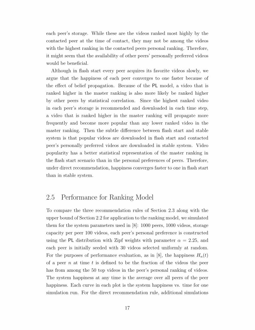
2.5 Performance for Ranking Model

To compare the three recommendation rules of Section 2.3 along with the

upper bound of Section 2.2 for application to the ranking model, we simulated

them for the system parameters used in [8]: 1000 peers, 1000 videos, storage

capacity per peer 100 videos, each peer’s personal preference is constructed

using the PL distribution with Zipf weights with parameter α = 2.25, and

each peer is initially seeded with 30 videos selected uniformly at random.

For the purposes of performance evaluation, as in [8], the happiness Hn(t)

of a peer n at time t is defined to be the fraction of the videos the peer

has from among the 50 top videos in the peer’s personal ranking of videos.

The system happiness at any time is the average over all peers of the peer

happiness. Each curve in each plot is the system happiness vs. time for one

simulation run. For the direct recommendation rule, additional simulations

17

are presented to evaluate the robustness of the performance.

2.5.1 Performance of MLE Recommendation Rule and UpperBounds

Figure 2.1 shows the happiness vs. time for (i) the MLE rule, (ii) the global

list recommendation rule with the adaptive linear choice of W , (iii) the upper

bound of Section 2.2, and (iv) the trivial upper bound of Section 2.2 (giving

rise to the straight line of slope 1/50). Both the MLE recommendation rule

and the global list recommendation rule give performance very close to the

upper bound, with the MLE having a slightly better performance than the

global list recommendation rule.

0 50 100 150 200 250 300 3500

0.2

0.4

0.6

0.8

1

Iterations

Norm

alized T

ota

l H

appin

ess

Global list updates: adaptive linearNo repeated downloads

MLE ignoringsampling bias

Peer knows true order,downloads from serverIdeal: peer

knowspreference

Figure 2.1: Video content collection performance with partial ranks andupper bounds in a system of 1000 peers, 1000 videos, 100 storage size, andk = 50

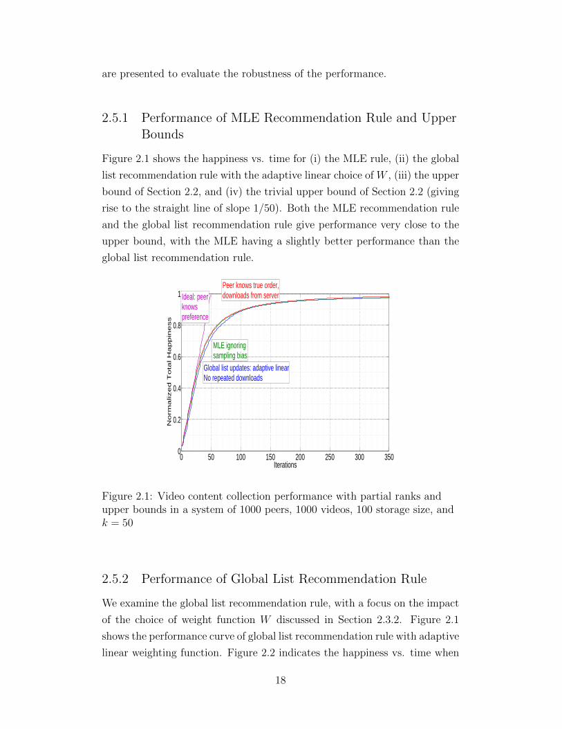
2.5.2 Performance of Global List Recommendation Rule

We examine the global list recommendation rule, with a focus on the impact

of the choice of weight function W discussed in Section 2.3.2. Figure 2.1

shows the performance curve of global list recommendation rule with adaptive

linear weighting function. Figure 2.2 indicates the happiness vs. time when

18

the weight function W used in the global list recommendation rule is Cruz’s

top-K weighting function with K = 50. Two curves are shown. For the

upper curve, peers do not download the same video twice. The performance

is sluggish for small t, which is to be expected; if a peer has at most K = 50

videos it will rate all of them in its top 50.1

Iterations0 50 100 150 200 250 300 350

No

rma

lize

d T

ota

l H

ap

pin

ess

0

0.2

0.4

0.6

0.8

1Global list updates: flat top 50No repeated downloads

Global list updates: flat top 50Repeated downloads permitted

Figure 2.2: Video content collection performance with Cruz’s binaryweighting function in a system of 1000 peers, 1000 videos, 100 storage size,and k = 50

The performance curves of the global list recommendation rule for all three

choices of weighting function W described in Section 2.3.2 are shown in

Figure 2.3. Both the positive linear W and the adaptive linear W perform

substantially better than the top-50 binary W, with adaptive linear doing

slightly better than positive linear.

2.5.3 Direct Recommendation - Robustness of Performance

In the simulations we have found that the direct recommendation rule per-

forms nearly as well as the more complex MLE recommendation rule or the

global list recommendation rule with positive linear or adaptive linear W .

1Simulation of the same system appears much better in Cruz’s paper, possibly due toleaking of master ranking information to peers during tie breaking.

19

Iterations0 50 100 150 200 250 300 350

No

rma

lize

d T

ota

l H

ap

pin

ess

0

0.2

0.4

0.6

0.8

1 Global list updates:adaptive linear

positive linear

flat top 50

Figure 2.3: Video content collection performance with linear weightingfunctions in a system of 1000 peers, 1000 videos, and 100 storage size

The performance curves are shown in Figure 2.4. In addition, the robustness

of the direct recommendation rule is explored under a variety of assumptions.

0 50 100 150 200 250 300 3500

0.2

0.4

0.6

0.8

1

Iterations

Norm

alized T

ota

l H

appin

ess

Global list updates: adaptive linearNo repeated downloads

Direct recommendation rule

Peer knows true order,downloads from server

Figure 2.4: Video content collection performance with directrecommendation in a system of 1000 peers, 1000 videos, 100 storage size,and k = 50

20

Varying α

Recall each peer’s personal preference is constructed using the PL ranking

model with Zipf weights wm ∝ m−α. The similarity among peers is increasing

in α. At the extreme value α = 0, the peers have independent preferences,

and at the extreme α → ∞ the peers have identical preferences. Figure 2.5

shows the upper bound and the performance of the direct recommendation

rule for α ∈ {2.25, 1.25, 0.8, 0.6, 0.2, 0}. The performance strongly depends

on α. However, it appears that the performance gap between the direct

recommendation rule and the upper bound is small over the complete range

of α, with the largest gap for α in the range 0.6 to 0.8. This illustrates

the robustness of the direct recommendation rule under different personal

preference distributions.

Iterations0 50 100 150 200 250 300 350

Norm

alized tota

l happin

ess

0

0.2

0.4

0.6

0.8

1Peer knows true order,downloads from server

1.25

2.25

0.8

0

0.2

0.6

Direct recommendation rule

Figure 2.5: Video content collection performance with directrecommendation in a system of 1000 peers, 1000 videos, and 100 storagesize, for several different Zipf parameter values

Varying Initial Video Availability

Recall each peer is initially seeded with 30 videos selected uniformly at

random. To check the performance of the direct recommendation rule at

different initial video availabilities, we have performed simulations with fewer

initial video availabilities at each peer. Figure 2.6 shows the performance

21

when each peer is initially seeded with 10, 5 or 1 videos selected uniformly

at random, respectively. It appears that the performance gaps of the direct

recommendation rule over different initial video availabilities are small when

each peer is initially seeded at least 5 videos. If each peer is seeded with only

one randomly selected video and M=N , then the probability a particular

video is initially present in the system is 1− (1− 1N

)N ≈ 1−e−1 ≈ 62%. This

limits the normalized total system happiness to about 62%. Figure 2.6 thus

shows near optimal performance for the direct recommendation rule even for

one initial available video per peer. This illustrates the robustness of the

direct recommendation rule under more restrictive initial video availabilities.

Iterations0 50 100 150 200 250 300 350

Norm

alized T

ota

l H

appin

ess

0

0.2

0.4

0.6

0.8

1

1

30

510

Figure 2.6: Video content collection performance with directrecommendation in a system of 1000 peers, 1000 videos, and 100 storagesizes, for several different initial video availabilities

Varying Storage Size

Recall each peer has a storage capacity of 100 videos. To check the per-

formance of the direct recommendation rule with different storage sizes, we

have performed simulations with smaller storage sizes at each peer. Figure 2.7

shows the performance when each peer has a storage capacity of 75, 50 or

30 videos, respectively. It appears that the performance gaps of the direct

recommendation rule over different storage sizes are small when storage sizes

22

are at least 50 videos, which is the threshold used in the happiness function.

If each peer has a storage capacity of 30 videos, which is the number of videos

initially available to each peer, then the normalized total system happiness is

limited to at most 3050

= 60%. Figure 2.7 thus shows near optimal performance

for the direct recommendation rule even for storage capacity of 30 videos per

peer. This illustrates the robustness of the direct recommendation rule under

more restrictive storage sizes.

Iterations0 50 100 150 200 250 300 350

Norm

alized T

ota

l H

appin

ess

0

0.2

0.4

0.6

0.8

1100

75

50

30

Figure 2.7: Video content collection performance with directrecommendation in a system of 1000 peers, 1000 videos, and various storagesizes

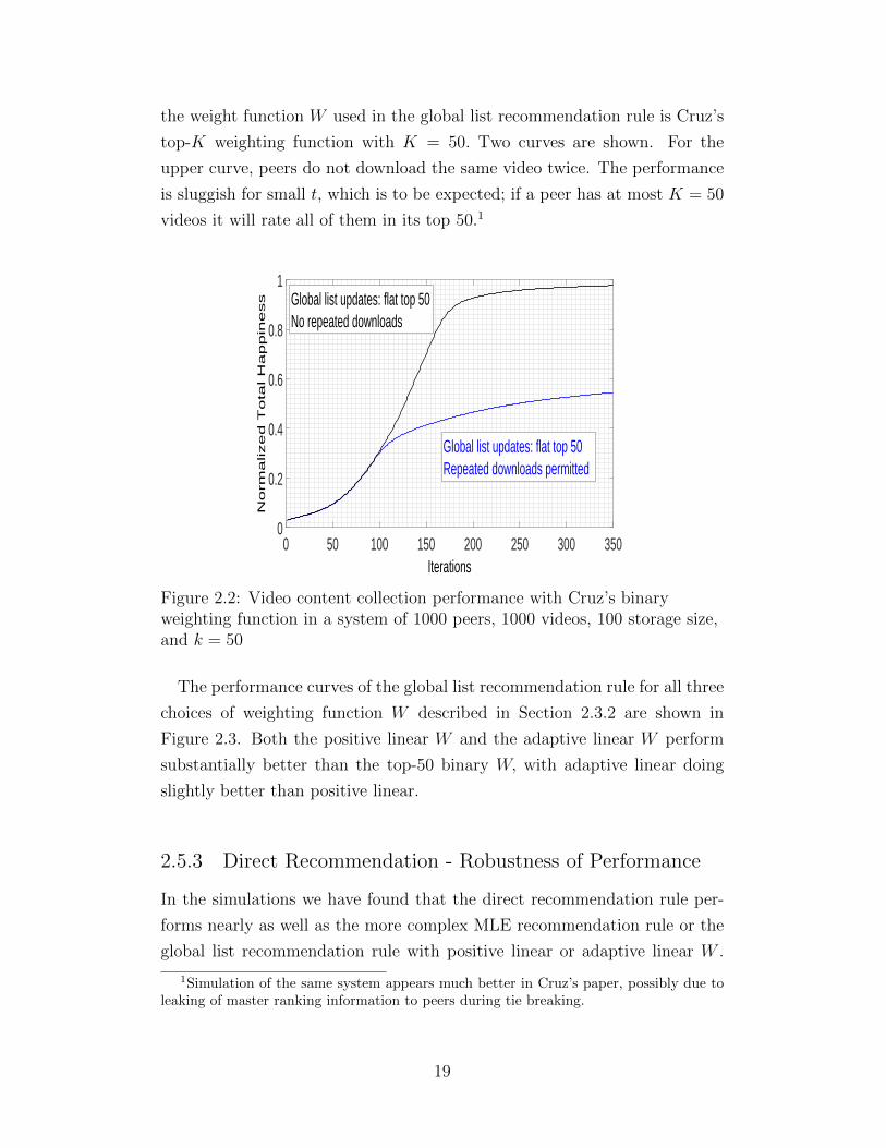
Variation: Peers Arriving to Stable System

To check the performance of the direct recommendation rule at different

peer arrival rates, we have performed simulations on a peer arriving under

two system scenarios: flash start and stable system. The corresponding

performance curves of the direct recommendation rule under the two system

states are shown in Figure 2.8.

The simulations give evidence in favor of our hypothesis that flash start

helps peers acquire their favored videos better than a stable system using the

direct recommendation rule due to the belief propagation effect (see Section

2.4), although the differences are small. This illustrates the robustness of the

23

0 50 100 150 200 250 300 3500

0.2

0.4

0.6

0.8

1

Iterations

Norm

alized T

ota

l H

appin

ess

Peer knows true order,downloads from server

Direct recommendation rulewith flash start

Direct recommendation rule, performanceseen by new peers in stable system

Figure 2.8: Effect of belief propagation for video content collection withdirect recommendation in a system of 1000 peers, 1000 videos, 100 storagesize, and k = 50

direct recommendation rule under the two extreme peer arrival patterns.

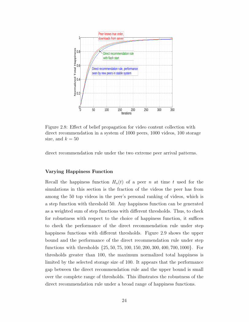
Varying Happiness Function

Recall the happiness function Hn(t) of a peer n at time t used for the

simulations in this section is the fraction of the videos the peer has from

among the 50 top videos in the peer’s personal ranking of videos, which is

a step function with threshold 50. Any happiness function can be generated

as a weighted sum of step functions with different thresholds. Thus, to check

for robustness with respect to the choice of happiness function, it suffices

to check the performance of the direct recommendation rule under step

happiness functions with different thresholds. Figure 2.9 shows the upper

bound and the performance of the direct recommendation rule under step

functions with thresholds {25, 50, 75, 100, 150, 200, 300, 400, 700, 1000}. For

thresholds greater than 100, the maximum normalized total happiness is

limited by the selected storage size of 100. It appears that the performance

gap between the direct recommendation rule and the upper bound is small

over the complete range of thresholds. This illustrates the robustness of the

direct recommendation rule under a broad range of happiness functions.

24

Iterations0 50 100 150 200 250 300 350

Norm

alized T

ota

l H

appin

ess

0

0.2

0.4

0.6

0.8

1

2550

75

150

200

300

400

7001000

100 Direct recommendation rule

Peer knows true order,downloads from server

Figure 2.9: Video content collection performance with directrecommendation in a system of 1000 peers, 1000 videos, and variousthresholds in happiness step functions

2.6 Summary of Results

In the single-cluster regime with homogeneous population and PL ranking

model, we analyzed the distributed recommendation system that jointly

performs content collection and rank aggregation. We found a performance

upper bound using stochastic comparison. Using the intuition obtained

from the performance upper bound, three recommendation rules of different

complexity are proposed. We proposed a deluxe recommendation rule that

estimates the master ranking using MLE. The deluxe recommendation rule

used the EM algorithm on partial rankings and was found to be near optimal

in the simulations. We reevaluated Cruz’s recommendation rule and obtained

insights in the global list recommendation rule and the weight functions.

With the intuition, we tried to optimize this approach and proposed more

efficient variations of the rule using different weighting functions to produce

an aggregate of partial rankings. Lastly, we proposed a simple greedy recom-

mendation rule called direct recommendation and found that its performance

is also near optimal in the simulations.

A main conclusion is that distributed content collection and rank aggrega-

tion is not only feasible, but the proposed direct recommendation rule works

25

remarkably well over a broad range of system parameters including strength

of correlation among peers, initial number of videos available, storage sizes,

peer arrival patterns, and choice of happiness functions. This conclusion is

illustrated by the simulations described in Section 2.5.3.

2.7 Derivation of EM Algorithm for Estimating the

Master Ranking

P. S. Efraimidis made the connection between WSNR and the collection of

independent exponential random variables [26]. Specifically, given a prob-

ability vector θ = (θ1, θ2, ..., θn), let X = {X1, X2, ..., Xn} be a vector of

independent exponential random variables with the given distribution rates

Xi ∼ Exp(θi) for 1 ≤ i ≤ n. The set of the exponential random variables

produces an ordered set of exponential jumps such that the orders follow the

same probability distribution as the order produced by WSNR. For example,

let n = 3 and suppose the order of exponential jumps is {X1, X3, X2},then X1 occurs before X2 and X3 with probability θ1

θ1+θ2+θ3, and by the

memoryless property of exponential random variable, X3 occurs before X2

with probability θ3θ2+θ3

.

Suppose we ignore the fact that θ in PL model is a permutation of the

Zipf distribution. Then, we have a convex problem to find MLE of θ. The

exponential representation will simplify the estimation method, i.e., the MM

algorithm can be reduced to the EM algorithm for our model.

For completeness, we derive the EM algorithm. Let θ = {θ1, θ2, ..., θ|M |}be the parameter to be estimated. The estimated parameters are the s-

caled Zipf parameters. Let X = {XCu(1),1, XCu(2),2, ..., XCu(t),t} be the com-

plete data, which is the vector of exponential variables sets with Zipf pa-

rameters as the rates, i.e. XCu(s),s = {x(Cu(s),m,s)|m ∈ |M |}. Let Y =

{PR1Cu(1)

, PR2Cu(2)

, ..., RV tCu(t)} be the observed direct ranking vectors. Let

PF tCu(t)

(r), 1 ≤ r ≤ VCu(t)(t), be the partial preference function, which is the

inverse of RV tCu(t)

. Then, the conditional probability of the complete data

given θ is Pcd(X|θ). We derive the expectation step and the maximization

step below.

26

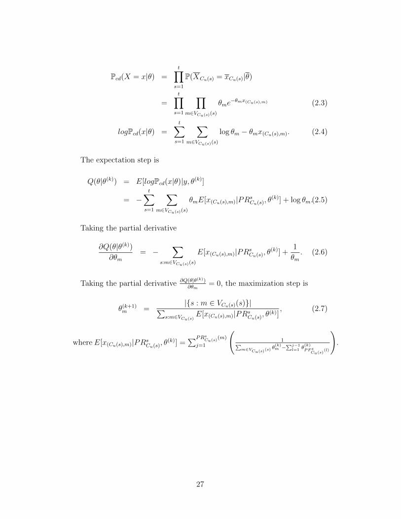
Pcd(X = x|θ) =t∏

s=1

P(XCu(s) = xCu(s)|θ)

=t∏

s=1

∏m∈VCu(s)(s)

θme−θmx(Cu(s),m) (2.3)

logPcd(x|θ) =t∑

s=1

∑m∈VCu(s)(s)

log θm − θmx(Cu(s),m). (2.4)

The expectation step is

Q(θ|θ(k)) = E[logPcd(x|θ)|y, θ(k)]

= −t∑

s=1

∑m∈VCu(s)(s)

θmE[x(Cu(s),m)|PRsCu(s), θ

(k)] + log θm.(2.5)

Taking the partial derivative

∂Q(θ|θ(k))∂θm

= −∑

s:m∈VCu(s)(s)

E[x(Cu(s),m)|PRsCu(s), θ

(k)] +1

θm. (2.6)

Taking the partial derivative ∂Q(θ|θ(k))∂θm

= 0, the maximization step is

θ(k+1)m =

|{s : m ∈ VCu(s)(s)}|∑s:m∈VCu(s)

E[x(Cu(s),m)|PRsCu(s)

, θ(k)], (2.7)

where E[x(Cu(s),m)|PRsCu(s)

, θ(k)] =∑PRs

Cu(s)(m)

j=1

(1∑

m∈VCu(s)(s)θ(k)m −

∑j−1l=1 θ

(k)

PFsCu(s)

(l)

).

27

CHAPTER 3

SCORING SYSTEM AND LARGE SYSTEMSCALING

An alternative to classifying videos by ranking them is for peers to classify

videos by assigning scores. We shall consider a model for correlated score

assignments by peers similar to the PL model for correlated rankings by peers.

At least for the direct recommendation rule, this provides some analytical

tractability, and, as shown in Section 3.5, the analysis can be applied back

to the PL ranking model.

3.1 Independent Crossover Channel Model

For the independent crossover (IC) channel model, there are L possible scores,

[L] = {1, ..., L}, for each video. Similar to the PL model, given a master

score vector, peers’ preferences are constructed so that they are conditionally

independent given the master score vector. To be consistent with the ranking

order in the previous sections, we let lower numbered scores represent more

preferred videos. Let M denote the number of videos and let G1, . . . , GL be

disjoint subsets of [M ], with union equal to [M ], and call the videos indexed

by G` type ` videos. This partition is equivalent to giving a master score

vector, where the video types are master scores. Let m` = |G`| for ` ∈ [L].

The IC channel model for L, G1, . . . , GL, and an L × L stochastic matrix

W is defined as follows. For any video in G`, a peer assigns personal score

`′ to the video with probability W``′ . The scores assigned by all peers to all

videos are assumed to be independent, given the types of the videos. Each

peer n for n ∈ [N ] has an intrinsic personal scores of videos, in : [M ]→ [L].

We can and do take the viewpoint that a peer decides what score to assign

to a video upon downloading the video.

The problem of distributed content collection and score aggregation among

N peers can be formulated for scores and the IC model just as it was for

28

rankings and the PL model. In particular, the happiness of a peer at time

t can be defined in terms of a happiness function, based on the scores of

the videos obtained by the peer up to time t. The direct recommendation

rule carries over with no change; when a peer contacts another peer, the

video downloaded is uniformly randomly selected from among the highest

scored (by the contacted peer) videos that are available at the contacted

peer and not yet possessed by the contacting peer. For analytical tractability

throughout the remainder of this section, we consider the IC model used under

the direct recommendation rule. We also show how the method can be applied

to give an approximate analysis for the PL ranking model used under the

direct recommendation rule.

If A,B are finite multisets of R, A � B (A is better than B) indicates

that |A| ≥ |B| and a[i] ≤ b[i] for 1 ≤ i ≤ |B|, where a[1] ≤ . . . ≤ a[|A|]

denotes the ordered elements of A and b[1] ≤ . . . ≤ b[|B|] denotes the ordered

elements of B. The happiness function of a peer at time t is defined as

Hn(t) = f({in(m) : m ∈ Sn(t)}), where f : 2[M | → R, is assumed to be

nondecreasing in the � order, and 2[M ] denotes the set of subsets of [M ].

3.2 An Upper Bound on System Performance

To obtain an upper bound on the happiness of a peer, no matter what

recommendation rule is used, consider an idealized system in which the peer

has access to a server that can provide any video, and for which a genie

reveals extra information. If the genie revealed to the peer the peer’s own

personal scores of the videos, (i(m) : m ∈ [M ]), then the obviously optimal

rule of the peer would be to download videos in the order of increasing

numerical personal scores. This provides a rather trivial upper bound on

the happiness of a peer vs. time. Our focus is on a tighter upper bound,

derived by considering the case in which the peer has access to a server, and

the genie reveals only the master scores to the peer. Since the preferences of

other peers in the system are conditionally independent given the master

scores, the scores of other peers provide no additional clues to the peer

about its own preferences. The following theorem shows the peer’s optimal

recommendation rule is to download the videos in the order of increasing

master score (e.g. increasing index m).

29

Theorem 3.2.1. Let f : 2[M ] → [0, 1] be nondecreasing in the happiness

order ≺ . Let (i(m) : m ∈ [M ]) denote a random scoring vector generated

by the IC model for some G1, ..., GL and W . Suppose the rows of W are

increasing in the usual stochastic order sense. If A,B ⊂ [M ] such that

A � B, then E [f({i(m) : m ∈ A})] ≥ E [f({i(m) : m ∈ B})] .

Proof of Theorem 3.2.1. Let a[1], ..., a[|A|] and b[1], ..., b[B] denote the ordered

elements of A and B respectively. By assumption, |A| ≥ |B| and a[m] ≤ b[m]

for 1 ≤ m ≤ |B|. Since the rows of W are nondecreasing in the stochastic

order sense, the scores (i(m) : m ∈ A) and (i(m) : m ∈ B) can be coupled

as follows. There exists (i′(m) : m ∈ A) and (i′′(m) : m ∈ B) on one

probability space such that (i) (i′(m) : m ∈ A)d.= (i(m) : m ∈ A), (ii)

(i′′(m) : m ∈ B)d.= (i(m) : m ∈ B), and (iii) P{(i′(m) : m ∈ A) � (i′′(m) :

m ∈ B)} = 1. Thus, P{f{i′(m) : m ∈ A}} ≤ f{i′′(m) : m ∈ B}} = 1, so

E[f{i′(m) : m ∈ A}] ≤ E[f{i′′(m) : m ∈ B}].

In words, if a set A of videos is better than a set B of videos in the

master order, then A is stochastically better than B for a peer. The bound

suggests that performance in the original system would be nearly optimal

if (1) the peers could quickly and accurately infer the master order by

sharing preference information, and (2) the peer-to-peer content distribution

mechanism could provide requested videos nearly as well as a centralized

server.

3.3 The Mean Field Limit (N →∞)

The state of the system at a given time consists of the states of all N peers.

Each peer has (L+1)M possible states, which we refer to as detailed states of

the peers. The detailed state of a peer can be written as i = (i(m) : m ∈ [M ])

where i(m) ∈ {0, . . . , L} indicates the score the peer assigns to video m, with

value zero denoting that the peer does not yet have the video. In a system of

N peers, let XNn (t) represent the state of peer n at time t. By definition, the

empirical distribution of peers in the system at time t, denoted by MN(t),

assigns probability MNi (t) = 1

N

∑Nn=1 1{XN

n (t)=i} to i for each possible detailed

state i of a peer. Then, each peer’s state transition probabilities given the

state of the system are denoted by KNij (~r) , P{XN

n (t + 1) = j| ~MN(t) =

30

~r,XNn (t) = i}, where ~r is a probability vector indexed by detailed states with

coordinates being a multiple of 1N

.

The number of possible system states, (L + 1)MN , grows exponentially

with N. Fortunately, because peers contact each other uniformly at random,

the ordering of peers is not relevant. By this exchangeability among peers,

the detailed state of the system at a given time can be represented by

the sequence of empirical distributions ( ~MN(t) : t ≥ 0), which forms a

Markov sequence. If we let N → ∞, we can apply mean field theory to

the system, implying that the empirical distribution becomes deterministic

by the following theorem.

Theorem 3.3.1. [27] Let (XNn (t) : t ≥ 0,∀n ∈ N) be a sequence of states

for objects in a system such that the sequence of the empirical distributions

of objects in the system ( ~MNi (t) : t ≥ 0) is a Markov sequence and the state

transitions for individual objects at time t+ 1 are conditionally independent

given the current state at time t. Suppose the transition probabilities have

the form P{XNn (t+ 1) = j| ~MN(t) = ~r,XN

n (t) = i} = KNij (~r). Assume for all

i, j, for N →∞, KNij (~r) converges uniformly in ~r to some Kij(~r), which is a

continuous function of ~r. Also assume that the initial empirical distribution~MN(0) converges almost surely to a deterministic limit ~µ(0). Define ~µ(t)

iteratively by its initial value ~µ(0) and for t ≥ 0:

~µj(t+ 1) =∑i

~µi(t)Kij(~µ(t)). (3.1)

Then for any fixed t ≥ 0, almost surely, limN→∞ ~MN(t) = ~µ(t).

Theorem 3.3.1 directly applies to the IC model with the direct recom-

mendation rule. For that application, KNij (~r) does not depend on N when

peers are allowed to contact themselves, so KNij (~r) ≡ Kij(~r). Since Kij(~r)

is a linear combination of the coordinates of ~r, it is a continuous function

of ~r. ~MN(0) is the empirical distribution of N i.i.d. random variables with

distribution not dependent on N ; we assume the same fraction of videos are

chosen uniformly at random to be initially stored in each peer. Therefore,~MN(0) = limN→∞ ~MN(0) a.s., where ~M(0) is the initial state distribution

for a peer. Theorem 3.3.1 gives rise to a mean field model, in which there is

a single tagged peer with a Markov evolution, such that for a time step from

t to t+ 1, the tagged peer interacts with a contacted peer selected using the

31

probability vector ~µ(t), independently of the past history of the tagged peer.

The vector ~µ(t) is also the distribution of the tagged peer at time t.

While the evolution of the empirical distribution of the detailed states is

deterministic in the limit N →∞, the number of possible states for a single

peer, (L+ 1)M , is still so large that solving the update equation (3.1) is not

computationally feasible for realistic choices of L and M. We next describe

how the state space can be reduced substantially by exploiting symmetry.

In the original system the initial distribution and the dynamics are invariant

with respect to reordering of the videos within each group G`, and that

invariance is inherited by the mean field limit. Specifically, if i is a possible

detailed state of a peer, let Z``′(i) be the number of videos the peer has

with master score ` and personal score `′. Define two states i and i′ to be

equivalent if Z(i) ≡ Z(i′). By the symmetry noted above, it follows that

~µi(t) = ~µi′(t). We refer to (Z``′(i) : `, `′ ∈ [L]) as the reduced state of a

peer. A peer has∏L

`=1

(L+m`m`

)possible reduced states. For the mean field

model, it suffices to track the probabilities of reduced states because the

probability of a detailed state can be recovered by dividing the probability of

its corresponding reduced state by the number of equivalent detailed states.

The sequence of reduced states of the tagged peer in the mean field model

continues to be a Markov process.

Another observation can be used to further reduce the number of states

considered. The determination of which video the tagged peer downloads

from a contacted peer does not involve how the tagged peer has rated its own

videos. Therefore, if (Z` : ` ∈ [L]) denotes how many videos the tagged peer

has from each of the master groups G` at some time t, the scores assigned to

those videos by the tagged peer are conditionally independent, with the scores

of videos in G` being assigned using the `th row of W. For determination of the

state of the tagged peer at time t+ 1, it does matter how the contacted peer

has rated the videos it has. But the distribution of the state of the contacted

peer is the same as that of the tagged peer, so the scores the contacted

peer has assigned to the videos it has from each master score group G` are

also conditionally independent and generated according to the `th row of W.

Equivalently, it is as if the contacted peer scores each of the videos it has from

each master group G` at the time of contact by the tagged peer. Therefore,

the mean field probability ~µ(t) can be computed by only keeping track of the

distribution of (Z` : ` ∈ [L]) for the tagged peer. Given (Z` : ` ∈ [L]) for a

32

peer at some time, the conditional distribution of detailed state is as follows.

Independently, for each `, the conditional distribution of the m` coordinates

(i(m) : m ∈ G`) is that there are m`−Z` zeros selected uniformly at random

from among the m` possible locations, and Z` nonzero scores, each selected

independently according to the `th row of W. We refer to (Z` : ` ∈ [L]) as the

more reduced state of a peer. There are∏L

`=1(m` + 1) possible more reduced

states.

In closing this section, we describe the mean field model for the more re-

duced states in more detail. It has the following parameters: positive integers

M,L,m1, . . . ,mL, such that M = m1+. . .+mL, an L×L crossover matrix W ,

and a constant c > 0 denoting the fraction of videos initially assigned to each

peer. We switch to using µ(M)t for the mean field limit distribution at time t,

to denote the dependence on M , in anticipation of the next section. The state

space for the model is S(M) ={z ∈ ZL+ : 0 ≤ z` ≤ m`

}. The dynamical aspect

of the mean field model is described by a function Φ(M) : S(M)×S(M) → Σ(L),

where Σ(L) = {p ∈ RL+ :∑

` p` ≤ 1}. The interpretation is that if the state

of the tagged peer is z and the randomly contacted peer has state z′, then

Φ(M)` (z, z′) is the probability that the tagged peer downloads a type ` video

from the contacted peer. The detailed specification of Φ(M)(z, z′) is a bit

complicated but can be briefly explained as an algorithm, as follows. Given

z and z′, first, for each `, generate a random variable representing the number

of type ` videos eligible for download, where eligible for download means three

conditions are satisfied: (i) the contacted peer has the video, (ii) the tagged

peer does not have the video, and (iii) the contacted peer classifies the video

as type 1 (true with probability W`1). If at least one video is eligible for

download, one such video is selected for download uniformly at random from

among those that are eligible. If no such videos are eligible, repeat steps (i)-

(iii) seeking a video of type 2 to download, and so on. If the contacted peer

has no video that the tagged peer does not have, no video is downloaded.

The mean field model determines a sequence (µ(M)t : t ≥ 0) of probability

distributions (represented as vectors) on S(M). These distributions are de-

termined recursively as follows. The initial distribution, µ(M)0 , corresponds

to selecting Mc videos uniformly at random from [M ] and recording the

number of each type selected. Given µ(M)t for some t ≥ 0, states Z and

Z ′, corresponding to a tagged peer and a contacted peer, are independently

generated with distribution µ(M)t , and then the video downloaded by the

33

tagged peer is determined using the distribution Φ(M)(Z,Z ′). If the video

is type `, the new state of the tagged peer Z is modified by increasing the

`th coordinate by one. Then, µ(M)t+1 is the probability distribution of the new

state of the tagged peer.

Once the sequence of distributions (µ(M)t : t ≥ 0) has been calculated,

we can define a Markov process modeling the entire time history, (Zt : t ≥0) = (Zt,` : t ≥ 0, ` ∈ [L]), of a tagged peer as follows. The initial state Z0

has distribution µ(M)0 , and, given Zt, the distribution of what type video is

downloaded to get Zt+1 is given by Φ(M,1,t)(Zt), where

Φ(M,1,t)(z) ,∑

z′∈S(M)

Φ(M)(z, z′)µ(M)t,z′ .

Like Φ(M), Φ(M,1,t) takes values in Σ(L). The “1” and “t” in the notation

Φ(M,1,t)(z) indicate that one argument of Φ(M)(z, z′) remains after z′, cor-

responding to the state of the contacted peer, is averaged out using the

distribution µ(M)t , which depends on t. Induction on t shows that Zt has

distribution µ(M)t for each t. This completes our description of the mean field

model.

3.4 Fluid Limit of the Mean Field Model (M →∞)

Although the number of possible more reduced states is much smaller than

the number of detailed states, it is still rather large and, furthermore, ex-

act computation of the state transition matrix for the more reduced states

essentially requires expanding to the reduced states and is computationally

expensive. For example, for 1000 videos, binary scores, and 50 videos with

the higher score, there are about 5 × 104 more reduced states, so the time

dependent transition probability matrix for the state of the tagged peer has

(5×104)2 entries. To reduce the complexity further we establish a fluid limit

of the mean field model as the number of videos converges to infinity. The

limit takes advantage of the fact, due to the law of large numbers, that the

distribution of the more reduced state of the tagged peer tends to concentrate

around its mean. This entails the limit of a limit, because the mean field

model itself arises as the number of peers converges to infinity.

Consider a sequence of mean field models as M → ∞ with L, c, and an

34

L × L crossover probability matrix W fixed. Also, let ρρρ = (ρ1, . . . , ρL) be

a fixed probability vector with positive coordinates, and let (m1, . . . ,mL)

depend on L in such a way that m` = ρ`M for ` ∈ [L]. To avoid trivial

complications, we assume Mc and m` for each ` are integer valued; this can

be done, for example, by assuming c and the coordinates of ρρρ are multiples

of 0.01 and M is a multiple of 100. Let

ϕ`(x, y) ,(1− x`/ρ`)y`W`1∑`′(1− x`′/ρ`′)y`′W`′1

and let (bτ : 0 ≤ τ ≤ (1−c)) denote the solution to bτ = ϕ(bτ , bτ ) with initial

state b0 = cρρρ. The following theorem is proved in Section 3.8.1.

Theorem 3.4.1. Suppose the first column of W has strictly positive entries.

As M → ∞, sup0≤t≤M(1−c) ‖ZtM − bt/M‖ → 0, where the convergence is in

probability.

The idea of the proof of Theorem 3.4.1 is as follows. Classical techniques

from the theory of differential equation limits of Markov processes (see for

example, [28] and the references therein) are applied to show that as M →∞,the scaled stochastic trajectory of Z concentrates along a deterministic path.

It follows that the peers contacted by the tagged peer also have states near the

same deterministic trajectory. The deterministic trajectory is identified by

drift analysis, which in the limit m→∞ after scaling in time and space gives

rise to the integral equation that is equivalent to the differential equation

determining b.

We next discuss the approximation suggested by Theorem 3.4.1. The

theorem shows that for large M , Zt is well approximated by zt , Mbt/M .

Expressing the differential equation for b in terms of z yields

zt,` =(1− zt,`

m`)zt,`W`1∑

`′(1−zt,`′

m`′)zt,`′W`′1

, z0 = ρρρMc. (3.2)

The righthand side of (3.2) has a natural interpretation. The numerator

represents the approximate number of videos from master group ` that are

eligible for transfer from the contacted peer, and the whole righthand side

represents the fraction of eligible videos that are from master group `. All

these videos are among those assigned score one by the contacted peer. By

35

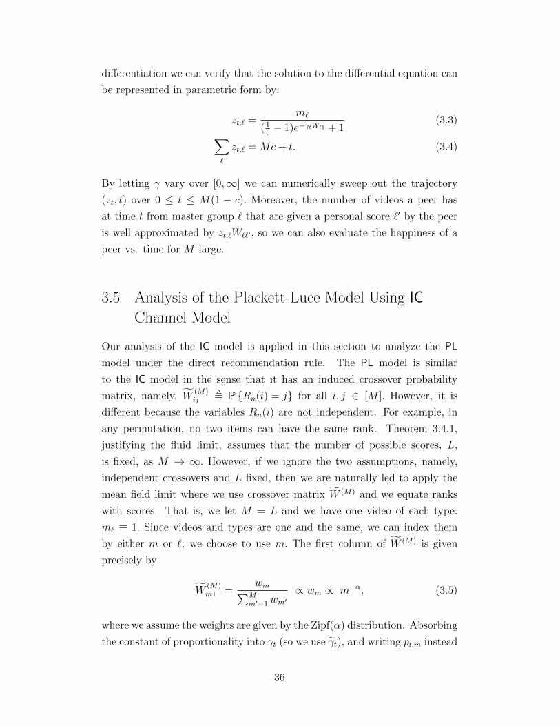
differentiation we can verify that the solution to the differential equation can

be represented in parametric form by:

zt,` =m`

(1c− 1)e−γtWl1 + 1

(3.3)∑`

zt,` = Mc+ t. (3.4)

By letting γ vary over [0,∞] we can numerically sweep out the trajectory

(zt, t) over 0 ≤ t ≤ M(1 − c). Moreover, the number of videos a peer has

at time t from master group ` that are given a personal score `′ by the peer

is well approximated by zt,`W``′ , so we can also evaluate the happiness of a

peer vs. time for M large.

3.5 Analysis of the Plackett-Luce Model Using IC

Channel Model

Our analysis of the IC model is applied in this section to analyze the PL

model under the direct recommendation rule. The PL model is similar

to the IC model in the sense that it has an induced crossover probability

matrix, namely, W(M)ij , P {Rn(i) = j} for all i, j ∈ [M ]. However, it is

different because the variables Rn(i) are not independent. For example, in

any permutation, no two items can have the same rank. Theorem 3.4.1,

justifying the fluid limit, assumes that the number of possible scores, L,

is fixed, as M → ∞. However, if we ignore the two assumptions, namely,

independent crossovers and L fixed, then we are naturally led to apply the

mean field limit where we use crossover matrix W (M) and we equate ranks

with scores. That is, we let M = L and we have one video of each type:

m` ≡ 1. Since videos and types are one and the same, we can index them

by either m or `; we choose to use m. The first column of W (M) is given

precisely by

W(M)m1 =

wm∑Mm′=1wm′

∝ wm ∝ m−α, (3.5)

where we assume the weights are given by the Zipf(α) distribution. Absorbing

the constant of proportionality into γt (so we use γt), and writing pt,m instead

36

of zt,`, we get the following expression for the probability a peer has videom at

time t for the PL model with Zipf(α) weights with the direct recommendation

rule:

pt,m =1

(1c− 1)e−γtm−α + 1

(3.6)∑m

pt,m = Mc+ t. (3.7)

In spite of the approximations we have made, comparison with simulations

in Section 3.6.3 suggests that (3.6)-(3.7) is rather accurate.

In the remainder of this section, we give a rigorous connection between the

PL model and IC model in the large M limit. To make a ranking model look

more like a score model it is natural to quantize ranks into a small number

of scores as follows. Let [L] = {1, . . . , L} be the set of possible scores, with

1 denoting the best score and L the worst score, and let ρρρ = (ρ1, . . . , ρL)

be a probability vector with strictly positive entries. Let {I1, . . . , IL} be

a partition of the interval [0, 1] into intervals such that I` has length ρ`.

Specifically, I1 = [0, ρ1], I2 = (ρ1, ρ1 + ρ2], I3 = (ρ1 + ρ2, ρ1 + ρ2 + ρ3] and

so on, and let ψ : [0, 1] → [L] be such that ψ(r) = ` for r ∈ I`. Map a

rank r ∈ [M ] into a score by applying ψ to the normalized rank, to get score

ψ(r/M). Let G` ={m ∈ [M ] : m

M∈ I`

}, which is the set of ranks in [M ] that

map to score `, and let m` = |G`|. It is easy to check that |m` − ρ`M | < 1

for all `. We assume the parameters (wm) are such that wm is decreasing

in m, so that the items are indexed according to some master order. It

is then natural to define the input score (or master score) of item m as

ψ(m/M). Thus, each item m has an input score ψ(m/M) and a random

output score ψ(R(m)/M). The PL model and quantization function ψ then

induce the crossover matrix W (M) obtained by tracking the scores of items

before and after the PL channel: W(M)``′ , 1

m`

∑m∈G` P {ψ(R(m)/M) = `′} .

That is, W(M)``′ is the probability that a randomly selected item with input

score ` is given output score `′. If L << M then there is little dependence

between the scores assigned to different items, given their input scores. The

following theorem states a precise form of this observation for the case that

the parameters w are given by a Zipf distribution: wm = (m/M)−α for some

α > 0. Since the PL model is invariant with respect to multiplicative scaling

of the w’s, this is equivalent to using parameters wm = m−α.

37

Define F∞(c) ,∫ 1

01− exp(−u−αc)du for c ≥ 0, and

W``′ ,1

ρ`

∫I`

P {F∞(xαZ) ∈ I`′} dx (3.8)

for `, `′ ∈ [L], where Z has the exponential probability distribution with

parameter one.1 The following theorem is proved in Section 3.8.2. It says

that for a fixed quantization function ψ, the quantized input and output

scores for a fixed number of videos under the PL model converge jointly in

distribution to the input and output scores for the same fixed number of

videos for the IC model.

Theorem 3.5.1. (Convergence of quantized PL to IC) Let α > 0 and for M ≥1 consider a random permutation R with the PL distribution with parameters

M and (wi = (i/M)−α : i ∈ [M ]). Fix a quantizer function ψ with parameters

L and ρρρ as described above. Fix K ≥ 1 and let A1, . . . , AK denote K indices

in [M ] selected uniformly at random without replacement. Note that ψ(Ai/M)

denotes the input score of item Ai and ψ(R(Ai)/M) denotes the output score

of item Ai.

Let (A1, . . . , AK , B1, . . . , BK) denote a vector of random variables such that

the K pairs (Ak, Bk), 1 ≤ k ≤ K, are mutually independent, and for each

k ∈ [K] : Ak has distribution ρρρ and P{Bk = j|Ak = i

}= Wij for i, j ∈ [L].

Then(ψ(A1

M

), . . . , ψ

(AKM

), ψ(R(A1)M

), . . . , ψ

(R(AK)M

))converges in dis-

tribution to (A1, . . . , AK , B1, . . . , BK) as M →∞.

Theorem 3.5.1 suggests a way to analyze the performance of the PL model

with a large number of peers and videos by approximating it by an IC model.

The idea is to adopt a quantizer function ψ, compute the corresponding

limiting crossover matrix W, and then use W in the mean field fluid limit

analysis given for the IC model.

Our experience with this approach and comparison with simulations showed

that the approximation improved as the number of levels L of the quantizer

increases; see Section 3.6.2. That led to the proposal to use M = L described

at the beginning of the section.

1The formula given for W is equivalent to W``′ , 1ρ`

∫I`×I`′

q(x, y)dxdy where, for each

x fixed, q(x, ·) is the pdf of the random variable F∞(xαZ). The function q is in a sensethe continuum limit of W as L→∞ with max` ρ` → 0.

38

3.6 Performance for Scoring Model

This section shows calculations and simulations that illustrate the mean field

and fluid limit convergence, and also illustrate how performance of the PL

model can be analyzed using the IC model. Then, the performance of the

fluid approximation is compared with the upper bound of Section 3.2. The

direct recommendation rule is assumed throughout. The model parameter

values are the same as used in [8] and Section 2.5: 1000 peers, 1000 videos, 30

random videos seeded per peer, Zipf parameter α = 2.25, with the exception

that the buffer space here is assumed to be unlimited. The happiness of a

peer at a given point in time is the fraction of videos it has with personal

score L∗ or better, among all videos with personal score L∗ or better, where

L∗ is such that the expected number of videos with personal score L∗ or

better is 50. Each curve in each plot is the system happiness vs. time for

one simulation run.

3.6.1 Direct Recommendation Rule with Binary Scores

To illustrate the mean field and fluid limit convergence for the IC model, we

consider the case of L = 2 and ρρρ = (0.050, 0.950). The 2×2 crossover matrix

W used is given by (3.8) for α = 2.25 and ρρρ. Namely,

W =

(0.7419 0.2586

0.0136 0.9864

).

Four performance curves are shown in Figure 3.1. One is the happiness for

a simulation of the entire system of 1000 peers, 1000 videos, with 50 type

1 videos. The second curve is the fluid approximation determined by (3.3),

(3.4), andW , as explained just after (3.4). The third curve is the performance

predicted by a hybrid between the pure mean field model and the fluid limit

of the mean field model, obtained as follows. Since L = 2, the more reduced

state of a peer has the form (z1, z2) ∈ {0, . . . , 50} × {0, . . . , 950}. For the

hybrid calculation we track the distribution of z1 which becomes a 51-state

Markov chain and we represent z2 by a deterministic real number updated by

drift analysis (similar to (3.13)). Thus, for each time step, the tagged peer

and contacted per have a random number of type 1 videos and a deterministic

39

number of type 2 videos, and the probability the tagged peer downloads a

type 1 video is calculated to get the peer distribution for the next time step.

The fourth curve is the upper bound of Section 3.2.

Examination of Figure 3.1 shows close agreement between the simulation

and the two numerically computed approximations to system happiness. In

addition, the direct recommendation rule with binary scores performs nearly

as well as the upper bound under IC model.

Iterations0 50 100 150 200 250 300 350

Norm

alized T

ota

l H

appin

ess

0

0.2

0.4

0.6

0.8

1

IC model with binaryscore and deterministichybrid dynamics

Simulation ofIC model withbinary score

IC model withbinary scoreand deterministicfluid dynamics

Peer knows true order,downloads from server

Figure 3.1: Video content collection performance with directrecommendation in a system of 1000 peers, 1000 videos, unlimited storagesize, and binary scores under IC model

3.6.2 Direct Recommendation Rule with Many Scores

Figure 3.2 shows the performance curves for the direct recommendation rule

under IC model for four different numbers of scores, L = 2, 3, 4, 1000. For

L = 2, 3, 4 the crossover matrix W is given by (3.8) with α = 2.25 and for

L = 1000 the crossover matrix is given by (3.5). In addition, the upper

bound of Section 3.2 is shown in the plot for L = 1000. The happiness

is calculated using the fluid approximation determined by (3.3), (3.4), and

W. The corresponding choices of Mρρρ, giving the number of videos in each

score group, are (50, 950), (50, 50, 900), (25, 25, 50, 900), and (1, 1, . . . , 1),

respectively.

40

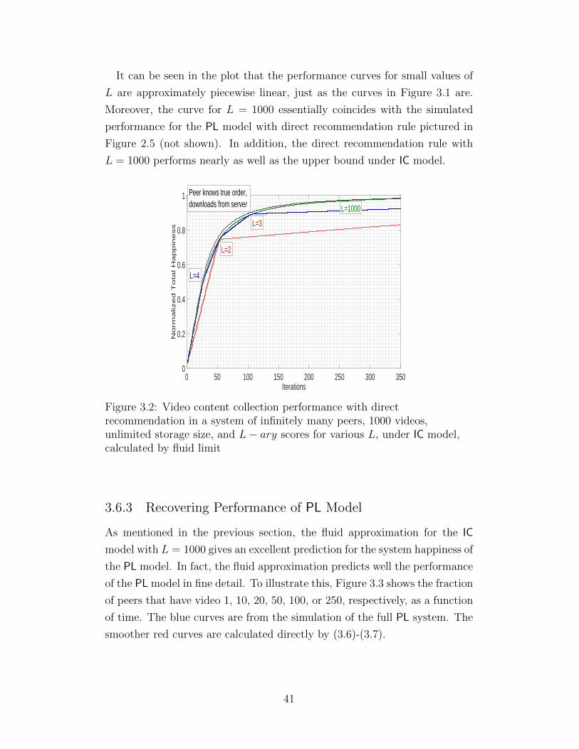
It can be seen in the plot that the performance curves for small values of

L are approximately piecewise linear, just as the curves in Figure 3.1 are.

Moreover, the curve for L = 1000 essentially coincides with the simulated

performance for the PL model with direct recommendation rule pictured in

Figure 2.5 (not shown). In addition, the direct recommendation rule with

L = 1000 performs nearly as well as the upper bound under IC model.

Iterations0 50 100 150 200 250 300 350

Norm

alized T

ota

l H

appin

ess

0

0.2

0.4

0.6

0.8

1

L=2

L=4

L=3

L=1000

Peer knows true order,downloads from server

Figure 3.2: Video content collection performance with directrecommendation in a system of infinitely many peers, 1000 videos,unlimited storage size, and L− ary scores for various L, under IC model,calculated by fluid limit

3.6.3 Recovering Performance of PL Model

As mentioned in the previous section, the fluid approximation for the IC

model with L = 1000 gives an excellent prediction for the system happiness of

the PL model. In fact, the fluid approximation predicts well the performance

of the PL model in fine detail. To illustrate this, Figure 3.3 shows the fraction

of peers that have video 1, 10, 20, 50, 100, or 250, respectively, as a function

of time. The blue curves are from the simulation of the full PL system. The

smoother red curves are calculated directly by (3.6)-(3.7).

41

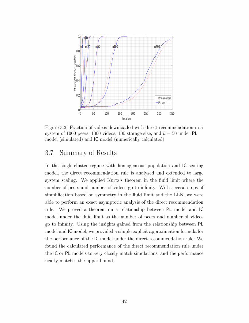
Iteration0 50 100 150 200 250 300 350

Fra

ction d

ow

nlo

aded

0

0.2

0.4

0.6

0.8

1

IC numericalPL sim

m20m1 m50 m100

m10

m250

Figure 3.3: Fraction of videos downloaded with direct recommendation in asystem of 1000 peers, 1000 videos, 100 storage size, and k = 50 under PLmodel (simulated) and IC model (numerically calculated)

3.7 Summary of Results

In the single-cluster regime with homogeneous population and IC scoring

model, the direct recommendation rule is analyzed and extended to large

system scaling. We applied Kurtz’s theorem in the fluid limit where the

number of peers and number of videos go to infinity. With several steps of

simplification based on symmetry in the fluid limit and the LLN, we were

able to perform an exact asymptotic analysis of the direct recommendation

rule. We proved a theorem on a relationship between PL model and IC

model under the fluid limit as the number of peers and number of videos

go to infinity. Using the insights gained from the relationship between PL

model and IC model, we provided a simple explicit approximation formula for

the performance of the IC model under the direct recommendation rule. We

found the calculated performance of the direct recommendation rule under

the IC or PL models to very closely match simulations, and the performance

nearly matches the upper bound.

42

3.8 Proofs of Limit Theorems

3.8.1 Proof of Theorem 3.4.1

To begin, we show that the distribution µ(M)0 of the initial state Z0 of the

tagged peer concentrates on a small subset of the state space. A random

variable X has the hypergeometric distribution with parameters n, k1, k2 if it

has the following interpretation. If k2 balls are drawn uniformly at random

without replacement from an urn initially containing n balls, of which k1 are

red, then X denotes the number of red balls drawn. Note that E [X] = k1k2n.

Hoeffding [29] showed that this distribution is convex order dominated by

the distribution that would result by sampling with replacement, namely,

by the binomial distribution, Binom(k2,

k1n

). In particular, since the square

function is convex, var(X) ≤ k2(k1n

)(1− k1n

) ≤ E [X] .2

By assumption, a peer initially has Mc videos, selected uniformly at ran-

dom from among all M videos, and for each ` ∈ [L], there are m` = ρlM

type ` videos (i.e. videos with master score `). Thus, the number of type `

videos the tagged peer initially has, denoted by Z0,`, has the hyperexponential

distribution with parameters M,Mc,Mρ`. By Hoeffding’s bound mentioned

above, E [‖Z0 − ρρρMc‖2] =∑

` var(Z0,`) ≤ Mc. Therefore, by the Markov

inequality, for any δ > 0, P {‖Z0 − ρρρMc‖ ≥ δM} ≤ cδ2M

M→∞−→ 0. That is,Z0

M→ ρρρc in probability as M →∞. This concentration result implies that the

initial state of any peer is greater than or equal to ρρρMc/2 coordinatewise with

probability converging to one. Since the states of peers are nondecreasing

with time, it follows that

inft≥0

∑z∈S(M):z≥ρρρMc/2

µ(M)t,z

M→∞−→ 1. (3.9)

Note that∑

` ϕ`(x, y) = 1 so that∑

` bt,` = c + t for 0 ≤ t ≤ 1 − c,

and b1−c = ρρρ. Therefore, to prove the theorem it suffices to show that for

2Hoeffding’s result also implies that Chernoff bounds for binomial distributions alsohold for the hypergeometric distribution. In particular, if X has a hypergeometricprobability distribution, the Chernoff bounds for binomial X imply (see Theorems 4.4

& 4.5 in [30]): P{∣∣∣∣ X

E[X] − 1

∣∣∣∣ ≥ ε} ≤ 2e−ε2E[X]/3, ∀0 ≤ ε ≤ 1. For simplicity in this

thesis, we will stick with bounds based on variance rather than exponential moments.

43

any fixed ε > 0, sup0≤t≤M(1−c−ε) ‖ZtM − bt/M‖ → 0. To this end, fix ε >

0 for the remainder of this proof. Consider the following subset of S(M):

S(M) ={z ∈ ZL+ : m`c/2 ≤ z` ≤ m` and

∑` z` ≤ (1− ε)M

}. We only need

to consider the system up until time M(1−c−ε) so that the upper constraint,∑` z` ≤ (1−ε)M, will not be violated by the state process of any peer. This,

together with (3.9), implies:

inf0≤t≤M(1−c−ε)

∑z∈S(M)

µ(M)t.z

M→∞−→ 1. (3.10)

In analogy with S(M) and S(M), let:

S(∞) = {x ∈ RL+ : 0 ≤ x` ≤ ρ`}

S(∞) = {x ∈ RL+ : cρ`/2 ≤ x` ≤ ρ` and

∑`

x` ≤ 1− ε}.

For x, y ∈ S(∞), the denominator of ϕ(x, y) is greater than or equal to

εcmin` ρ`W`1/2, and hence, bounded away from zero. It follows that ϕ and

its first derivatives over S(∞) × S(∞) are bounded and continuous. Let ϕ be

defined with domain S(∞) such that ϕ = ϕ over the set S(∞) × S(∞), and ϕ

and its first derivatives are bounded and continuous over S(∞) × S(∞). Since

bt ∈ S(∞) for 0 ≤ t ≤ 1−c−ε, we can also view b as the solution to b = ϕ(b, b)

with b0 = cρρρ.

We show in this paragraph that

supz,z′∈S(M)

∥∥∥∥Φ(M)(z, z′)− ϕ(z

M,z′

M

)∥∥∥∥→ 0 as M →∞. (3.11)

Since z, z′ ∈ S(M) implies zM, z′

M∈ S(∞), the meaning of (3.11) is unchanged

if ϕ is replaced by ϕ. To verify the claim, fix z, z′ ∈ S(M) and consider the

number of videos of some type ` eligible for transfer, assuming the tagged

peer has state z and the contacted peer has state z′. The number of type `

videos that (i) the contacted peer has and (ii) the tagged peer does not have,

denoted by N`, has the hyperexponential distribution with mean(Mρ`−z`)z′`

Mρ`.

In turn, given N`, the number of type ` videos eligible for transfer has the

Binom(N`,W`1) distribution, with mean(Mρ`−z`)z′`W`1

Mρ`≥ (Mρ` − z`)

cW`1

2,

where we used the fact z′` ≥ Mρ`c/2. The sum of these means is greater

44

than or equal to (M −∑

` z`)cmin`W`,1

2≥ M(1−ε)cmin`W`,1

2, where we used

the fact∑

` z` ≤ (1 − ε)M. Moreover, by the Chebychev inequalities for

hyperexponential and binomial random variables, the numbers of eligible

videos of each type are within δM of their means with high probability, for

arbitrarily small δ > 0. Therefore, the distribution of the type of the video

to be transferred is, in the limit m→∞, proportional to the means, namely,

it is given by ϕ(zM, z′

M

). Moreover, the estimates involved are uniform in

z, z′ ∈ S(M), implying (3.11) as claimed.

In analogy to the definition of Φ(M,1,t), let

ϕ(M,1,t)(x) ,∑

z′∈S(M)

ϕ

(x,z′

M

)µ(M)t,z′ . (3.12)

Let (B(M)t : 0 ≤ t ≤ M(1 − ε − t)) denote the deterministic, discrete-time

trajectory in RL+ defined recursively as follows:3

B(M)t =

t−1∑s=0

ϕ(M,1,s)

(B

(M)s

M

)+Mcρρρ. (3.13)

Next, we use arguments from the classical theory of limits of Markov

processes, to show that the trajectory of the Markov process Z closely follows

B with high probability. Adding and subtracting various terms and arranging

them yields:

Zt =t−1∑s=0

ϕ(M,1,s)

(ZsM

)

+t−1∑s=0

[Φ(M,1,s)(Zs)− ϕ(M,1,s)

(ZsM

)]+Mcρρρ+Mt. (3.14)

Mt =∑t−1

s=0

(Zs+1 − Zs − Φ(M,1,s) (Zs)

)+M0, and M0 = Z0 −Mcρρρ. The

process (Mt) is a mean zero Martingale. As explained near the beginning

of the proof, Hoeffding’s result yields E [‖M0‖2] ≤ Mc∑

` ρ`(1− ρ`) ≤ Mc.

Also, ‖Mt+1−Mt‖2 = ‖Zt+1−Zt−Φ(M,1,t)(Zt)‖2 ≤ 2 with probability one.

Furthermore, the increments of square integrable Martingales are orthogonal

3By convention,∑t−1s=0 is zero for t = 0.

45

random variables. Thus,

E[‖Mt‖2

]= E

[‖M0‖2

]+

t−1∑s=0

E[‖Ms+1 −Ms‖2

]≤Mc+ 2t.

Therefore, using Doob’s L2 inequality,

E

[sup

0≤s≤M(1−ε−c)‖Ms‖

2

]≤ 4E

[‖MM(1−ε−c)‖

2]≤ 8M.

Hence, if δ > 0 is a small fixed constant, by the Markov inequality,

P

{sup

0≤s≤M(1−ε−c)‖Ms‖ ≥

δM

2

}≤ 32

δ2M→ 0 as M →∞.

By (3.10), (3.11), and the boundedness of Φ and ϕ, it follows that the norm

of the quantity in square brackets in (3.14) is at most δ/2 for M sufficiently

large. Hence, (3.14) yields that, with probability converging to one as M →∞,

Zt =t−1∑s=0

ϕ(M,1,s)

(ZsM

)+Mcρρρ+ et, (3.15)

where ‖et‖ ≤ δM for 0 ≤ t ≤M(1− ε− c). Since ϕ has bounded derivatives,

the derivatives of ϕ(M,1,s) are uniformly bounded over all s, so that ϕ(M,1,s) is

cL-Lipschitz continuous for all s for some finite constant cL. So, subtracting

the respective of sides of (3.13) from (3.15) and using ‖et‖ ≤ δM yields that

‖Zt −B(M)t ‖ ≤ cL

M

t−1∑s=0

‖Zs −B(M)s ‖+ δM.

Thus, by induction on t, ‖Zt−B(M)t ‖ ≤ (1+ cL

M)tδM ≤ exp( cLt

M)δM. Therefore,

with probability converging to one as M →∞,

sup0≤t≤M(1−ε−c)

∥∥∥∥ZtM − B(M)t

M

∥∥∥∥ ≤ ecLδ. (3.16)

Next, we revisit the definition (3.12) of ϕ(M,1,t). It shows that ϕ(M,1,t)(x) is

obtained by averaging out y in ϕ(x, y) using the probability distribution of

46

Zt/M. But (3.16) shows that Zt/M is close to B(M)t /M with high probability.

It follows that for any δ > 0,

∥∥∥∥ϕ(M,1,t)(x) − ϕ(x,

B(M)t

M

)∥∥∥∥ → 0 as M → ∞,

uniformly over x ∈ S(∞) and t ∈ [0,M(1− ε− c)]. Applying this observation

to (3.13) then yields

B(M)t

M=

1

M

t−1∑s=0

ϕ

(B

(M)s

M,B

(M)s

M

)+ cρρρ+ e′t, (3.17)

where max0≤t≤M(1−ε−c) ‖e′t‖ → 0 as M → ∞. Introduce time scaling by

letting τ = t/n and b(M)τ =

B(M)Mτ

Mif τ is a multiple of 1/M and defining

b(M)τ elsewhere on [0, 1 − ε − c] by linear interpolation. Since ϕ is bounded

the functions b(M)τ are uniformly Lipschitz continuous, and hence by the

Arzela-Ascoli theorem, any subsequence has a convergent sub-subsequence.

By (3.17), any limit trajectory b(∞) satisfies

b(∞)τ =

∫ τ

0

ϕ(b(∞)σ , b(∞)

σ )dσ + cρρρ.

This integral equation has a unique solution, namely, b(∞) = b, so the entire

sequence b(M) converges uniformly to b asM →∞. So, sup0≤t≤M(1−ε−c) ‖B

(M)t

M−

bt/M‖ → 0, which, together with (3.16), implies Theorem 3.4.1.

3.8.2 Proof of Theorem 3.5.1

Using the exponential representation for the PL distribution with parameter

vector w1, . . . , wM , we can assume that R(m) is the rank of Xm among the in-

dependent random variables X1, . . . , XM , such that Xm is exponentially dis-

tributed with rate parameter wm for each m. Let FM(c) , 1M

∑m∈[M ] I{Xm≤c}.

That is, FM is the empirical cumulative distribution function of (Xm : m ∈[M ]). Notice that for any item m, R(m)

M= FM(Xm). That is, the rank of m,

normalized by division by M, is gotten by applying the function FM to Xm.

So FM is a stochastic ranking scale that maps X values into normalized ranks.

The following lemma shows that for large M , FM is well approximated by

F∞, which acts as a deterministic ranking scale.

Lemma 3.8.1. Let wm = (m/M)−α and

47

F∞(c) =∫ 1

01− exp(−u−αc)du. Then for any δ > 0,4

P{

supc≥0|FM(c)− F∞(c)| ≤ δ

}→ 1. (3.18)

Proof. By its definition, FM(c) for a fixed value of c, is the average of

M independent random variables, where the mth random variable has the

Bernoulli distribution with parameter 1− exp(−(m/M)−αc). Since Riemann

sums converge to integrals and can be bounded by integrals:

E[FM(c)

]=

1

M

M∑m=1

(1− exp(−(m/M)−αc)→ F∞(c)

var(FM(c)) ≤ 1

M2

M∑m=1

(1− exp(−(m/M)−αc) ≤ F∞(c)

M≤ 1

M,

it follows that, by the Chebychev inequality, FM(c)→ F∞(c) in distribution

as M →∞ for any fixed c. Select ci so that F∞(ci) = δi/2 for integers i with

1 ≤ i < 2/δ. Since the number of values of i is fixed, it follows that P {Eδ} →1 where Eδ , {maxi |FM(ci) − F∞(ci)| ≤ δ/2}. Furthermore, since FM is a

nondecreasing function and F∞ is a continuous, strictly increasing function,

both with range [0, 1], the event Eδ implies that supc≥0 |FM(c)−F∞(c)| ≤ δ,

so that (3.18) holds as claimed.

Proof of Theorem 3.5.1. We shall use a particular representation of (Ak, Bk).

Let U1, . . . , UK each be uniformly distributed on the interval [0, 1] and let

Z1, . . . , ZK each be exponentially distributed with mean one, and suppose

U1, . . . , UK , Z1, . . . , ZK are mutually independent. Then we can assume that

Ak = ψ(Uk) and Bk = ψ ◦ F∞(Uαk Zk). That is, with this representation,

the pairs (Ak, Bk), 1 ≤ k ≤ K are independent, the variables ψ(Uk) have

distribution (ρ1, . . . , ρK), and P{Bk = `′|Ak = `

}= W``′ (to prove the last

property, use the fact that given Ak = i, Uk is uniformly distributed over Ii).

A version of the continuous mapping theorem of measure theory (e.g. see

[31]) states that if a sequence of random vectors Vn converges in distribution

to a random vector V∞, and if φ is a Borel measurable function such that

P {V∞ ∈ Dφ} = 0, where Dφ is the set of discontinuity points of φ, then

4This is a variation of the Glivenko-Cantelli theorem; here the X’s are not identicallydistributed.

48

φ(Vn) converges in distribution to φ(V∞). In view of the continuous mapping

theorem, it suffices to prove(A1

M, . . . ,

AKM

,R(A1)

M, . . . ,

R(AK)

M

)d.→ (U1, . . . , UK , F∞(Uα

1 Z1), . . . , F∞(UαKZK)) (3.19)

as M → ∞. Indeed, applying the function φ : [0, 1]2K → [L]2K defined by

φ(x1, . . . , x2K) = (ψ(x1), . . . , ψ(x2K)) to the vectors on each side of (3.19)

makes the distributions of the corresponding sides match the distributions of

the vectors in the last sentence of Theorem 3.5.1. Since the random vector

on the righthand side of (3.19) has a joint probability density function, the

probability the vector is in Dφ is zero.

It remains to prove (3.19), and for that we use a coupling argument. First,

the random variable Ak for k ∈ [K] has the same distribution as dUkMe.So we can let Ak = dUkMe for all k in the event that the random variables

dUkMe are distinct, which has probability of converging to one as M →∞.That is, we can assume that the random vector (A1, · · · , AK) for each M and

the random vector (U1, . . . , UK) are all constructed on the same probability

space so that

P {Ak = dUkMe : 1 ≤ k ≤ K} ≥(

1− K

M

)KM→∞→ 1.

In particular, if follows that AkM→ Uk in the sense of convergence in proba-

bility, for each k. For the PL model, once the items A1, . . . , AK are selected,

exponential random variables (i.e. XAk : 1 ≤ k ≤ K) must be generated

for these items, as well as for all the other items. We can assume without

loss of generality that these exponential random variables are taken to be(AkM

)αZk : 1 ≤ k ≤ K, where (Z1, . . . , ZK) are the same exponential random

variables used for the representations of the B’s and appearing in (3.19).

Then R(Ak)M

= FM((

AkM

)αZk). Recall that P {Eδ} → 0 as M → ∞, and

49

|FM(c)− F∞(c)| ≤ δ for all c on the event Eδ. Thus, on the event Eδ,∣∣∣∣R(Ak)

M− F∞(Uα

k Zk)

∣∣∣∣=

∣∣∣∣FM ((dUkMeM

)αZk

)− F∞(Uα

k Zk)

∣∣∣∣≤ δ +

∣∣∣∣F∞((dUkMeM

)αZk

)− F∞(Uα

k Zk)

∣∣∣∣. (3.20)

By continuity of F∞, the second term in (3.20) converges to zero almost surely

as M → ∞, and hence also in the sense of convergence in probability. And

since δ > 0 is arbitrary, it follows that

∣∣∣∣R(Ak)M−F∞(Uα

k Zk)

∣∣∣∣→ 0 in probability

for each k. Thus (3.19) holds in the sense of convergence in probability, and

hence, also in distribution.

50

CHAPTER 4

THE MULTI-CLUSTER FRAMEWORK

Real world populations are usually heterogeneous. In order to model hetero-

geneous preferences, we consider a multi-cluster model for correlated score

assignments by peers and use insights gained from the single-cluster model

in Chapter 2 and Chapter 3 to propose distributed recommendation rules in

the multi-cluster regime.

We briefly compare centralized and distributed recommendation for multi-

cluster systems. For a centralized system, where all peers’ partial scoring

preferences are accessible, the central tracker can apply clustering algorithms

like the K-means heuristic to solve for the clustering problem, which includes

estimating the cluster centers’ score vectors. Once each peer knows its cluster

center score vector, it downloads videos from the central server according to

the preference order of its cluster center scores because of the stochastic

dominance property of PL with Zipf distribution, stated in Theorem 2.2.1.

For a distributed system which is the focus of this work, there are problems

of both limited preference information and limited video availability. Each

peer can be either selfish or helpful. If a peer is selfish, it first collects

preference information and estimates its cluster center score vector. Then

it downloads videos from its contacted peers according to the preference

order of its estimated cluster center scores. If a peer is helpful, it gathers

more preference information from contacted peers and passes on preference

information to contacted peers. Then it performs clustering on the collect-

ed preferences to identify every cluster center score vector. It downloads

videos based on the estimated cluster center scores to allow videos which are

commonly preferred among multiple clusters to disseminate faster; i.e., peers

cooperate to emulate a central tracker.

51

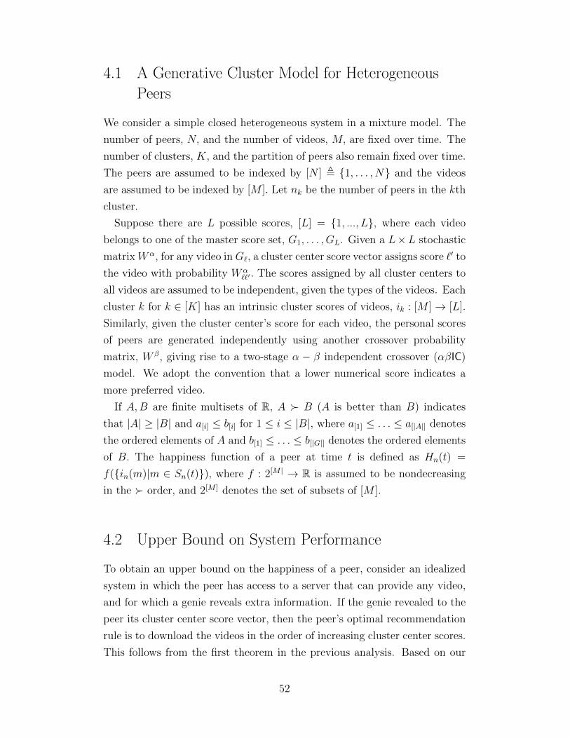
4.1 A Generative Cluster Model for Heterogeneous

Peers

We consider a simple closed heterogeneous system in a mixture model. The

number of peers, N, and the number of videos, M, are fixed over time. The

number of clusters, K, and the partition of peers also remain fixed over time.

The peers are assumed to be indexed by [N ] , {1, . . . , N} and the videos

are assumed to be indexed by [M ]. Let nk be the number of peers in the kth

cluster.

Suppose there are L possible scores, [L] = {1, ..., L}, where each video

belongs to one of the master score set, G1, . . . , GL. Given a L×L stochastic

matrix Wα, for any video in G`, a cluster center score vector assigns score `′ to

the video with probability Wα``′ . The scores assigned by all cluster centers to

all videos are assumed to be independent, given the types of the videos. Each

cluster k for k ∈ [K] has an intrinsic cluster scores of videos, ik : [M ]→ [L].

Similarly, given the cluster center’s score for each video, the personal scores

of peers are generated independently using another crossover probability

matrix, W β, giving rise to a two-stage α − β independent crossover (αβIC)

model. We adopt the convention that a lower numerical score indicates a

more preferred video.

If A,B are finite multisets of R, A � B (A is better than B) indicates

that |A| ≥ |B| and a[i] ≤ b[i] for 1 ≤ i ≤ |B|, where a[1] ≤ . . . ≤ a[|A|] denotes

the ordered elements of A and b[1] ≤ . . . ≤ b[|G|] denotes the ordered elements

of B. The happiness function of a peer at time t is defined as Hn(t) =

f({in(m)|m ∈ Sn(t)}), where f : 2[M | → R is assumed to be nondecreasing

in the � order, and 2[M ] denotes the set of subsets of [M ].

4.2 Upper Bound on System Performance

To obtain an upper bound on the happiness of a peer, consider an idealized

system in which the peer has access to a server that can provide any video,

and for which a genie reveals extra information. If the genie revealed to the

peer its cluster center score vector, then the peer’s optimal recommendation

rule is to download the videos in the order of increasing cluster center scores.

This follows from the first theorem in the previous analysis. Based on our

52

mixture model assumptions, this upper bound performance of the multi-

cluster model is statistically the same as the upper bound performance of

the single-cluster model in Section 3.2.

4.3 Clustering: Similarity Measures and Error

This section explores similarity measures between two partial preference

vectors and investigates whether two such vectors can be inferred to be from

peers in the same cluster based on their similarity.

4.3.1 The Potential for Clustering Assuming the αβIC Model

In multi-cluster systems, the rate at which a peer contacts another peer

from the same cluster is reduced in proportion to the fraction of peers in

the contacting peer’s cluster. To provide better recommendations when

contacted peers are in different clusters, it might be beneficial if peers use rec-

ommendation rules more complex than direct recommendations, specifically,

rules that perform clustering.

With the assumption that clusters are planted, the clustering problem is

the task of identifying which cluster each peer belongs to. If PL with Zipf

distribution induced crossover probability matrices are used, we can roughly

identify the difficulty of the clustering problem given the Zipf parameters.

For simplicity, we denote the Zipf parameters for the crossover probability

matrices Wα and W β as α and β respectively. When α is large, cluster

centers are more correlated than when α is small. If β is small, then personal

preferences of the same cluster are more scattered than when β is large. In

this combination of α and β, the clustering problem seems to be more difficult

than other combinations of α and β. In contrast, when α is small and β is

large, the clustering problem seems to be easier than other combinations of

α and β.

Note that if α is sufficiently large, although it is difficult to cluster pref-

erences, it is easy to find a near optimal recommendation rule because the

multi-cluster recommendation problem approximately reduces to the single-

cluster recommendation problem that we have previously studied. If β

is sufficiently small, it is also difficult to cluster preferences, because the

53

preferences are very scattered. In this case, the lack of correlations among

preferences cannot provide enough useful inference information, so recom-

mendation rules might not work well. Since some choices of α and β present

difficulty in clustering, we choose to analyze the distributed recommendation

system under α < β with moderate values.

4.3.2 Generic Similarity Measures for Clustering

Before analyzing the recommendation rules for the distributed system, we

study clustering measures on the mixture model to gain insight into clus-

tering. One way to make clustering decisions is to use distance or similarity

measures and a threshold. The calculations of distance or similarity measures

described here do not depend on Wα, W β, or clusters sizes (fraction of peers

in each cluster), although the thresholds will depend on these quantities. We

define the following distance and similarity measures which are commonly

used for scores (references), the normalized Euclidean distance and the cosine

similarity. The normalized Euclidean distance between two partial preference

vectors iu and iv is defined as

d(iu, iv) =

√∑m∈Su∩Sv(iu(m)− iv(m))2

|Su ∩ Sv|

and the cosine similarity between two partial preference vectors is defined as

s(iu, iv) =

∑m∈Su∩Sv iu(m)iv(m)√∑

m∈Su∩Sv iu(m)2√∑

m∈Su∩Sv iv(m)2,

where Su and Sv are the nonzero indices of the two partial preference vectors.

Because of the heavy tailed Zipf distribution and the choices of α and β,

in particular α < β, preferences under different clusters are less correlated

and thus more likely to yield larger differences in video scores. Normalized

Euclidean distance, which is more sensitive to the magnitude of the vectors,

would tend to result in a larger separation between two preferences from

different clusters compared to cosine similarity, which is more sensitive to

the angle between the vectors. For example, suppose in one case peer u

has (1, 5) and peer v has (5, 1) as scores for two common videos and in

another case peer u has (2, 10) and peer v has (10, 2) as scores for the two

54

videos. In both cases the cosine similarities are the same but the Euclidean

distances are different. According to our model assumptions and choices of

α and β, the second pair of preferences, (2, 10) and (10, 2), are less likely to

belong to the same cluster compared to the first pair, (1, 5) and (5, 1). An

example of Euclidean distance and cosine similarity is plotted in Figure 4.1

and Figure 4.2 between the partial preference vector of a peer from cluster 1

and the partial preference vectors of 1000 peers from clusters 1 to 10, ordered

with intervals of 100 peers in each cluster. Notice that the decision line on

the cosine similarity plot and the decision line on the normalized Euclidean

distance plot intersect nearly identical sets of peers, so only the distance

metric will be used in the following sections.

Peer Index0 100 200 300 400 500 600 700 800 900 1000N

orm

alized S

quare

d E

uclidean D

ista

nce

0.5

1

1.5

2

2.5

3

3.5

4

4.5

Figure 4.1: Normalized squared Euclidean distance between a peer fromcluster 1 and the rest

4.3.3 Model-Based Similarity Measure for Clustering

Suppose Wα, W β, prior distribution of master scores (fraction of videos in

each master score) and prior distribution of clusters (fraction of peers in

each cluster) are known, we can make clustering decisions by hypothesis

testing. The multi-cluster mixture model is shown in Figure 4.3. The

α channel between the master score vector and each cluster center score

vector is characterized by crossover probability matrix Wα and the β channel

55

Peer Index0 100 200 300 400 500 600 700 800 900 1000

Cosin

e S

imilarity

0.85

0.9

0.95

1

Figure 4.2: Cosine similarity between a peer from cluster 1 and the rest

between a cluster center score vector and each personal preference vector is

characterized by W β. We let H1 denote the hypothesis that the contacted

peer v is in the same cluster as the contacting peer u and H0 denote the

hypothesis that the contacted peer v is in a different cluster.

Master Scores

Cluster 1

Cluster K

Peer 1

Peer n

Peer N

Figure 4.3: Multi-cluster channel

When the contacting peer and the contacted peer share common videos, we

can calculate the posterior probability of the two hypotheses. Because of the

independent crossover channels, the following is true under either hypothesis:

The observed scores of the contacted peer are conditionally independent

given the scores of the contacting peer. The conditional probabilities of

the observed scores of the contacted peer given the scores of the contacting

peer under each hypothesis is thus the product of the conditional probability

for each video over all the common videos. Looking at a single video, the

56

conditional probability of observing score j from the contacted peer when

the contacting peer rates it score i under hypotheses H1 and H0 are shown

as follows:

H1 : PH1(j|i) =∑`

W β`iρ(`)W β

`j∑`′ ρ(`′)W β

`′i

(4.1)

H0 : PH0(j|i)

=∑m

(∑o

(∑`

W β`iρ(`)∑

`′ ρ(`′)W β`′i

Wαo`ρ(o)∑

o′ ρ(o′)Wαo′`

)Wαom

)W βmj, (4.2)

where ρ(`) is the prior distribution of score ` for 1 ≤ ` ≤ L. Recall that PL

induced matrices preserve the distributions of scores, so the distribution of

personal scores, cluster center scores and master scores are the same.

The posterior probabilities of H1 or H0 can be calculated as the product

of the conditional probability in (4.1) or (4.2) and the prior distribution of

clusters. When the two peers share multiple videos, the posterior probability

of each hypothesis is multiplicative over the set of common videos, shown as

follows:

H1 : P (H1|~i,~j) =PH1(~j|~i)P (H1)

ρ(~j)=

∏m PH1(j(m)|i(m)) · P (H1)

ρ(~j)(4.3)

H0 : P (H0|~i,~j) =PH0(~j|~i)P (H0)

ρ(~j)=

∏m PH0(j(m)|i(m)) · P (H0)

ρ(~j). (4.4)

4.3.4 Clustering Error

In multi-cluster systems, preference information is more useful if the prefer-

ences belong to peers who are similar to the contacting peer. Under a flash

start regime, peers share few common videos with each other. Since clustering

is based on the personal scores of the common videos shared between the

peers, it takes a long time for them to collect enough preference information

57

for the contacting peer to cluster. If the peers could view a common set of

test videos, it would speed up the clustering phase, which would allow peers

to quickly identify preferences that belong to their own clusters.

Having multiple common videos between peers decreases the decision error.

In hypothesis testing, the decision error based on a single common video can

be upper bounded in terms of the Bhattacharyya coefficient [32]. Given that

the contacting peer rates the video score i, the Bhattacharyya coefficient

is ρi ,∫ √

PH0(`|i)PH1(`|i)d`, where PHh(`|i) is the conditional probability

that the contacted peer rates the video score l under hypothesis h ∈ {0, 1}described in (4.1) and (4.2). The upper bound for the decision error is given

as Pe(π|i) ≤√π0π1ρi, where πh is the prior distribution of hypotheses H0

and H1. Based on the choice of Wα and W β, the decision error based on a

single common video can be calculated with respect to the personal scores

of the contacting peer. For example, when α = 0.8 and β = 2.25, the

Bhattacharyya coefficient is

ρi = [0.6706, 0.7982, 0.8464, 0.8782, 0.9108, 0.9379, 0.9623, 0.9763, 0.9783, 0.9554],

corresponding to the contacting peer’s personal scores i = [1, 2, ..., 10] respec-

tively.

To upper bound the decision error on multiple common videos, notice

that only the Bhattacharyya coefficient needs to be changed to PHh(~|~i)since the observed personal scores of the videos from the contacted peer are

conditionally independent given the hypothesis and the personal scores of the

contacting peer. The Bhattacharyya coefficient for a set of common videos

is thus the product of the ρi’s, PHh(~|~i) =∏

m PHh(`(m)|i(m)). Because the

Bhattacharyya coefficient is multiplicative, the upper bound of the decision

error decreases exponentially. Peers can make clustering decisions with high

accuracy after viewing just a small set of common videos. In the following

section, a small set of common videos are given to each peer to view initially.

58

4.4 Recommendation Rules Based on Stored Partial

Preference Vectors

One performance benchmark is when peers do not cluster and follow the

simple direct recommendation rule as if the contacted peer is in the same

cluster. This recommendation rule performs poorly for the multi-cluster

system, because the rate of downloading videos from other peers with similar

preferences is very low. This section describes recommendation rules for

which peers collect partial preference vectors of other peers.

Each peer stores a set of partial preference vectors that is updated each

time the peer contacts another peer. We consider two possibilities for how

aggressively peers collect partial preference vectors:

Linear Collection of Partial Preference Vectors

When a peer contacts another peer, the contacted peer’s preference vector

is first added to the set of vectors stored by the contacting peer. If the

number of stored partial preference vectors exceeds a maximum storage size,

the vector least similar to the contacting peer’s preference vector is removed.

We call this the least similar preference (LSP) storage management policy.

Since at most one partial preference vector is added per contact, the number

of stored vectors increases linearly until the maximum storage size is reached.

Exponential Collection of Partial Preference Vectors

With just a small set of partial preference vectors, few videos have sufficiently

many scores for accurate score prediction. To increase the accuracy of

recommendations, more preference information can be collected. For this

method, when a peer contacts another peer, the entire set of stored partial

preference vectors from the contacted peer is collected. This allows the

amount of preference information at each peer to grow exponentially in time

until the maximum storage size is reached. Each peer essentially emulates the

server’s role in collecting preference information and estimating its personal

preference, except the peer is still restricted to collect videos from the peers

it contacts. Because there are more available partial preference vectors as a

result of the exponential collection of partial preference vectors, it makes

sense to increase the storage capacity at each peer while still using the

LSP storage management policy. Also, more restrictive thresholds can be

59

applied in recommendation rules to yield more accurate score prediction.

Recommendation rules based on the lists of stored partial preference vectors

are described next.

4.4.1 Nearest Stored Preference Recommendation Rule

A simple rule using the list of stored partial preference vectors is the nearest

stored preference recommendation rule. For this rule, peer clustering and

video selection are done in a two-step procedure, followed each time a peer

contacts another peer.

Step 1) Based on the fact that preference information from another peer is

more valuable if it is more correlated with the contacting peer’s preference,

the contacting peer is likely to learn more about its own preferences from

more correlated preferences. In the first step, the strength of correlation

between the contacting peer’s preference vector and each of its stored partial

preference vectors is calculated by the distance metric or the model-based

similarity measure, described in Section 4.3.

Step 2) The contacting peer selects the most similar partial preference vec-

tor from its stored set. The videos with numerically higher (bad) scores are

filtered out from this partial preference vector, so only videos with sufficiently

good scores are considered. Then, the contacting peer downloads from the

contacted peer’s available videos following the order of the filtered partial

preference vector. If no videos can be selected due to the unavailability at

the contacted peer, the next most similar partial preference vector is selected

and filtered. This process continues until the contacting peer finds a video

to download from the contacted peer.

4.4.2 Bayesian Recommendation Rules

Bayesian Recommendation Rule with Soft Clustering

We next describe a two-step procedure in which all sufficiently similar pref-

erence vectors from the contacting peer’s stored set are identified and then

combined to estimate the cluster center scores for the contacting peer. The

first step is calculating the strength of correlation between the contacting

60

peer’s preference vector and each of its stored partial preference vectors.

The second step is combining stored scoring preference information and

estimating which video to download. Details are as follows:

Focusing on a contacting peer, denoted by peer u, let PS be peer u’s set

of stored partial preference vectors. We split each partial preference vector

from the set PS into two subvectors as follows: one with preferences for

videos that peer u has rated and the other with preferences for videos that

peer u has not rated. Let PSR denote the set of subvectors for videos peer

u has rated and let PSNR denote the set of subvectors for videos peer u has

not rated. Let iu be the partial preference vector of peer u and cu be peer

u’s cluster center score vector. Following the same partition as above, let iu,r

and cu,r denote the parts of iu and cu restricted to the domain of videos peer

u has rated and let iu,nr and cu,nr denote the parts of iu and cu restricted to

the domain of videos peer u has not rated yet.

Step 1) For each preference vector is ∈ PS, the probability is is in the same

cluster as peer u is calculated. Recall that for a given is, H0,s is the hypothesis

that is is in a different cluster from peer u, and H1,s is the hypothesis that is

is in the same cluster as peer u. The strength of correlation between peer u’s

preference vector and each stored partial preference vector is is calculated

independently using the posterior probabilities of hypotheses H0,s and H1,s.

Note that to calculate the posterior probabilities of hypotheses H0,s and H1,s

for each stored partial preference vector, it suffices to use the corresponding

partial preference vector from PSR and iu,r. Thus, we apply (4.3) and (4.4)

and substitute ~i = iu,r and ~j = is,r ∈ PSR to get P (H1,s|is,r, iu,r) and

P (H0,s|is,r, iu,r).Step 2) Peer u downloads video with the highest posterior expected hap-

piness. The posterior expected happiness for a particular video m not yet

viewed by peer u can be calculated from the posterior distribution of peer

u’s personal score of the video and the happiness function. The posterior

distribution of peer u’s personal score of each video is based on the posterior

distribution of peer u’s cluster center score of the video and the crossover

probability matrix W β. Therefore, given the happiness function and W β,

in order to determine which video to download, it suffices to calculate the

posterior distribution of peer u’s cluster center score for each video. We

explain how to do that next.

Following (4.1) and (4.2) with a slight modification, given the cluster center

61

score of video m is a, the likelihood of observing score b from a stored partial

preference vector is under hypothesis H1,s or H0,s respectively, is shown as

follows:

H1,s : PH1,s(b|a) = W βab (4.5)

H0,s : PH0,s(b|a) =∑a′

(∑o

Wαoaρ(o)Wα

oa′∑o′ ρ(o′)Wα

o′a

)W βa′b. (4.6)

Combining (4.5) and (4.6) for the video, given peer u’s cluster center score

of video m is a, the likelihood of observing score b for video m in vector is is

as follows:

P (b|a, is,r, iu,r) = PH0,s(b|a) · P (H0,s|is,r, iu,r)

+PH1,s(b|a) · P (H1,s|is,r, iu,r) (4.7)

Combining the entire set of stored partial preference vectors for video m,

given peer u’s cluster center score of video m is a, the likelihood of observing

the scores over the set of stored partial preference vectors is as follows:

P (PSNR(m)|a, PSR, iu,r) =∏is∈PS

P (is,nr(m)|a, is,r, iu,r).

Applying the Bayes rule, the posterior probability of score cu,nr(m) of peer

u’s cluster center score for an unrated video m, given the observations from

the set of stored partial preference vectors, is as follows:

P (cu,nr(m) = a|PS, iu,r) =P (PSNR(m)|a, PSR, iu,r) · ρ(a)∏

is∈PS ρ(is,nr(m)). (4.8)

Combining (4.8) with the happiness function and W β, we obtain the

expected happiness for each video that the contacting peer has not rated.

The peer then downloads an available video from the contacted peer with

62

the highest expected happiness. Here we have made the approximations that

each peer’s stored partial preference vectors are independent and scores of

videos are independent when calculating the posterior probability distribu-

tion of the cluster center scores.

Bayesian Recommendation Rule with Hard Clustering

The previous Bayesian recommendation rule can be modified to become a

Bayesian recommendation rule with hard decision. The first step of the two-

step procedure is the same as before; the strength of correlation between the

contacting peer’s preference vector and each of its stored partial preference

vectors is calculated independently. The second step is similar to the nearest

stored preference recommendation rule because this rule also filters informa-

tion. This recommendation rule makes a hard decision and ignores the stored

partial preference vectors that are not sufficiently similar to the contacting

peer, i.e. the stored partial preference vectors that are not likely to be in the

same cluster as the contacting peer. The second step is also similar to the

Bayesian recommendation rule with soft decision because this rule combines

stored partial preference vectors to estimate which video to download, but

only on the set of stored partial preference vectors that are similar to the

contacting peer. Details are as follows:

Step 1) For each preference vector is ∈ PS, the probability is is in the same

cluster as peer u is calculated using the posterior probability of hypotheses

H0,s and H1,s, i.e. P (H0,s|is,r, iu,r) and P (H1,s|is,r, iu,r).Step 2) Declare is is from the same cluster as peer u if P (H1,s|is,r, iu,r)

exceeds a threshold. The threshold is set by the Neyman-Pearson criteria,

being sufficiently large to restrict the probability of false alarm to be low, so

the remaining set of stored partial preference vectors is very likely to be in the

same cluster as the contacting peer. Let PSS ⊆ PS denote the remaining

set of stored partial preference vectors.

Peer u downloads video with the highest posterior expected happiness. The

posterior expected happiness for a particular video m not yet viewed by peer

u can be calculated from the posterior distribution of peer u’s cluster center

score, the happiness function, and W β. In contrast to the soft clustering rule,

this recommendation rule calculates the posterior distribution of peer u’s

cluster center score for each video based on PSS, which is assumed to contain

63

partial preference vectors only in peer u’s cluster after the hard decision.

Then for is ∈ PSS, we use P (H0,s|is,r, iu,r) = 0 and P (H1,s|is,r, iu,r) = 1

and (4.7) becomes P (b|a, is,r, iu,r) = PH1,s(b|a). Combining the set PSS for

video m, given peer u’s cluster center score of video m is a, the likelihood of

observing the scores over PSS is as follows:

P (PSSNR(m)|a) =∏

is∈PSS

PH1,s(is,nr(m)).

Applying Bayes rule, the posterior probability of score cu,nr(m) of peer u’s

cluster center score for an unrated video m, given the observations from the

set of stored partial preference vectors in the same cluster as the contacting

peer, is as follows:

P (cu,nr(m) = a|PSS, iu,r) =P (PSSNR(m)|a) · ρ(a)∏

is∈PSS ρ(is,nr(m)). (4.9)

Combining (4.9) with the happiness function and W β, we obtain the

expected happiness for each video that the contacting peer has not rated.

The peer then downloads an available video from the contacted peer with

the highest expected happiness. Here we have made the approximations that

each peer’s stored partial preference vectors are independent and scores of

videos are independent when calculating the posterior probability distribu-

tion of the cluster center scores.

4.5 Multi-Cluster Aware Global List Recommendation

Rule

In all previously discussed recommendation rules, each peer collects multiple

partial preference vectors. The stored partial preference vectors are then

processed to determine which video to download. A minimalistic approach

without the need to store partial preference vectors is to recursively combine

them. We call this recommendation rule the multi-cluster aware global list

recommendation rule, and we denote the aggregate of the partial preference

vectors the global list, which follows from Cruz [8]. Each peer maintains

64

one global list, denoted by gu. A peer’s global list is a set of L vectors of

tallies, in which the mth tally of the `th vector, gu(`,m), stores the number

of partial preference vectors observed so far that belong to the same cluster

as the contacting peer and have rated score l for video m.

The multi-cluster aware global list recommendation rule is a two-step

procedure executed when one peer contacts another. The first step is for the

contacting peer to update its global list. The second step is for the contacting

peer to estimate which video to download. Focusing on a contacting peer u,

details are as follows:

Step 1) The strength of correlation between peer u’s preference vector and

the contacted peer’s preference vector is calculated by the distance metric

or the model-based similarity measure. A hard decision is made using a

threshold to ignore the contacted peer’s preference vector if it belongs to

a different cluster. If the contacted peer’s preference vector belongs to the

same cluster as peer u, peer u’s global list is updated as follows: for each

video m ∈ [M ], gu(`,m) is incremented by one if the contacted peer rates

video m score ` ∈ [L].

Step 2) Similar to before, peer u downloads the video with the highest

posterior expected happiness. The posterior expected happiness of a partic-

ular video m not yet viewed by peer u can be calculated from the posterior

distribution of peer u’s cluster center score, the happiness function, and

W β. The difference is that this recommendation rule calculates the posterior

distribution of peer u’s cluster center score for each video based on the L

corresponding tallies from its global list, denoted by gu(m) = {gu(`,m) : ` ∈[L]}. Given peer u’s cluster center score of video m is a, the likelihood of

observing the L corresponding tallies is as follows:

P (gu(m)|a) =∏`∈[L]

P (`|a)gu(`,m).

Applying the Bayes rule, the posterior probability distribution of score

cu,nr(m) of peer u’s cluster center score for an unrated video m, given the L

corresponding tallies from its global list, is as follows:

65

P (cu,nr(m) = a|gu(m)) =P (gu(m)|a) · ρ(a)∏

`∈[L] ρ(`)gu(`,m). (4.10)

Combining (4.10) with the happiness function and W β, we obtain the

expected happiness for each video that the contacting peer has not rated.

The peer then downloads an available video from the contacted peer with

the highest expected happiness. Here we have made the approximation that

the contacted peers are distinct so the contacting peer’s global list is recur-

sively updated without checking for duplicate partial preference vectors and

scores of videos are independent when calculating the posterior probability

distribution of the cluster center scores.

Note that the multi-cluster aware global list recommendation rule is almost

exactly the same as the Bayesian recommendation rule with hard clustering,

because both recommendation rules have the same hard clustering in step

1 and the same Bayesian recommendation rule to calculate the posterior

distribution of each peer’s cluster center scores. The subtle difference is in

the Bayesian recommendation rule with hard clustering; each peer calcu-

lates the posterior distribution of its cluster center scores based on a set

of stored partial preference vectors with LSP storage management policy.

In the multi-cluster aware global list recommendation rule, because of the

aggregated tallies, each peer effectively calculates the posterior distribution

of its cluster center scores based on the partial preference vectors from all

of its contacted peers that are sufficiently similar. The multi-cluster aware

global list recommendation rule is the same as the Bayesian recommendation

rule with hard clustering with unlimited storage of partial preference vectors

and without LSP storage management policy.

4.6 Performance for Multi-Cluster Scoring Model

To compare the recommendation rules described in Section 4.4 along with the

upper bound of Section 4.2 for application to the scoring model, we simulated

them for the system parameters similar to the ones used in [8] and Section 3.6:

1000 peers, 1000 videos, and 30 random videos seeded per peer. In addition,

10 random common videos are seeded for each peer. Each peer obtains

66

the preference vector of its contacted peer and stores at most 30 preference

vectors with LSP storage management policy. For the generative cluster

model, the Zipf parameters are α = 0 and β = 2.25, so the cluster centers

are well separated. We assign scores to the videos from {1, ..., L} with L = 10

and distribution ρ = (0.025, 0.025, 0.025, 0.025, 0.5, 0.5, 0.1, 0.1, 0.3, 0.3). The

10×10 crossover matrices Wα and W β used are given by (3.8). The happiness

of a peer at a given point in time is the fraction of videos it has with personal

score L∗ = 2 or better, so the expected number of videos with personal score

L∗ = 2 or better is 50. Each curve in each plot is the system happiness vs.

time for one simulation run.

4.6.1 Benchmarks

Before simulating the proposed recommendation rules, we would like to check

the impact of multi-clusters on the distributed recommendation system. To

illustrate the difference between multi-cluster and single-cluster, two bench-

marks are shown. Given a genie telling each peer its cluster center score

vector, the first benchmark is the upper bound described in Section 4.2,

when peers download according to their cluster center’s score vectors from

the server. This is the same upper bound shown in the single-cluster section.

The second benchmark is when peers download according to the simple

direct recommendation rule described in Section 4.4, which is the same

rule described in the single-cluster section, but applied on the multi-cluster

system. The performance curves are shown in Figure 4.4. We observe a

large gap between the performance of the direct recommendation rule and

the upper bound.

4.6.2 Nearest Stored Preference Recommendation Rule

Recall that the nearest stored preference recommendation rule stores prefer-

ence vectors from all of the peer’s previously contacted peers up to the storage

constraint and performs a simple filtering algorithm. It is very similar to the

direct recommendation rule because both recommendation rules utilize a

simple greedy filtering algorithm. The major difference is that the nearest

stored preference recommendation rule stores multiple preference vectors so

67

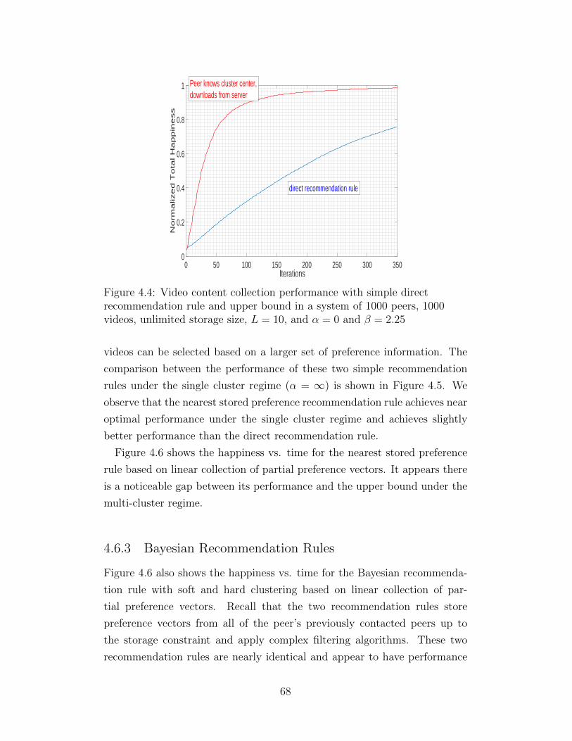
Iterations0 50 100 150 200 250 300 350

No

rma

lize

d T

ota

l H

ap

pin

ess

0

0.2

0.4

0.6

0.8

1 Peer knows cluster center,downloads from server

direct recommendation rule

Figure 4.4: Video content collection performance with simple directrecommendation rule and upper bound in a system of 1000 peers, 1000videos, unlimited storage size, L = 10, and α = 0 and β = 2.25

videos can be selected based on a larger set of preference information. The

comparison between the performance of these two simple recommendation

rules under the single cluster regime (α = ∞) is shown in Figure 4.5. We

observe that the nearest stored preference recommendation rule achieves near

optimal performance under the single cluster regime and achieves slightly

better performance than the direct recommendation rule.

Figure 4.6 shows the happiness vs. time for the nearest stored preference

rule based on linear collection of partial preference vectors. It appears there

is a noticeable gap between its performance and the upper bound under the

multi-cluster regime.

4.6.3 Bayesian Recommendation Rules

Figure 4.6 also shows the happiness vs. time for the Bayesian recommenda-

tion rule with soft and hard clustering based on linear collection of par-

tial preference vectors. Recall that the two recommendation rules store

preference vectors from all of the peer’s previously contacted peers up to

the storage constraint and apply complex filtering algorithms. These two

recommendation rules are nearly identical and appear to have performance

68

Iterations0 50 100 150 200 250 300 350

No

rma

lize

d T

ota

l H

ap

pin

ess

0

0.2

0.4

0.6

0.8

1

Nearest stored preference

Peer knows true order,downloads from server

Direct recommendation rule

Figure 4.5: Video content collection performance with nearest storedpreference recommendation rule in a system of 1000 peers, 1000 videos,unlimited storage size, L = 10, and α =∞ and β = 2.25

similar to that of the nearest stored preference rule.

Iterations0 50 100 150 200 250 300 350

No

rma

lize

d T

ota

l H

ap

pin

ess

0

0.2

0.4

0.6

0.8

1 Peer knows cluster center,downloads from server

Bayesian methodw/ hard clustering

Bayesian methodw/ soft clustering

Nearest stored preference

Figure 4.6: Video content collection performance with nearest storedpreference recommendation rule and Bayesian recommendation rule withsoft and hard clustering in a system of 1000 peers, 1000 videos, unlimitedstorage size, L = 10, and α = 0 and β = 2.25

69

4.6.4 Multi-Aware Global List Recommendation Rule

Figure 4.7 shows the happiness vs. time for the multi-cluster aware global

list recommendation rule based on linear collection of partial preference

vectors. Recall that the recommendation rule requires only the space for

one preference vector to store the aggregate preference information from the

peer’s previously contacted peers and applies complex filtering algorithm. It

appears to have performance similar to that of the nearest stored preference

rule.

Iterations0 50 100 150 200 250 300 350

No

rma

lize

d T

ota

l H

ap

pin

ess

0

0.2

0.4

0.6

0.8

1 Peer knows cluster center,downloads from server

Nearest stored preference

Global listmethod

Figure 4.7: Video content collection performance with nearest storedpreference recommendation rule and multi-cluster aware global listrecommendation rule in a system of 1000 peers, 1000 videos, unlimitedstorage size, L = 10, and α = 0 and β = 2.25

4.6.5 Cluster Correlations

To check the performance of the recommendation rules under more similar

personal preference distribution under the generative cluster model, the Zipf

parameter α is changed from 0 to 0.8 to yield correlated cluster centers.

When α is 0, the cluster centers are uniformly random. When α is 0.8,

the cluster centers are slightly correlated. Figure 4.8 shows the performance

of the recommendation rules described in Section 4.4 when α = 0.8 and

based on linear collection of partial preference vectors. In the simulation,

70

the nearest stored preference rule performs the best, displaying its robustness

against varying personal preference distributions similar to the robustness of

the direct recommendation rule in the single-cluster regime. The Bayesian

recommendation rule performs slightly better with soft clustering than with

the hard clustering. The global list recommendation rule performs the worst.

The Bayesian recommendation rules and the global list recommendation rule

did not perform well, perhaps because when cluster centers are closer togeth-

er, preference information outside of the contacting peer’s cluster is more

likely to introduce noise in combining preference information to estimate

which video to download. In contrast, for the nearest stored preference rule,

preference information is not combined.

Iterations0 50 100 150 200 250 300 350

No

rma

lize

d T

ota

l H

ap

pin

ess

0

0.2

0.4

0.6

0.8

1 Peer knows cluster center,downloads from server

Global listmethod

Bayesian methodw/ hard clustering

Bayesian methodw/ soft clustering

Nearest stored preference

Figure 4.8: Video content collection performance with multi-cluster awarerecommendation rules in a system of 1000 peers, 1000 videos, unlimitedstorage size, L = 10, and α = 0.8 and β = 2.25

4.6.6 Exponential Collection of Partial Preference Vectors

To reduce the performance gap between the recommendation rules and the

upper bound, partial preference vectors are collected exponentially in time.

We relax the storage constraint for preference vectors and assume the band-

width incurred from the exchange of preference information is negligible.

Then, each peer collects both its contacted peers’ personal preference vec-

71

tor and its contacted peers’ stored partial preference vectors. Figure 4.9

shows the happiness vs. time for the multi-cluster aware recommendation

rules with exponential collection of partial preference vectors described in

Section 4.4. The three performance curves with exponential collection of

partial preference vectors appear to be significantly closer to the upper bound

compared to without exponential collection of partial preference vectors. Of

the three recommendation rules, the Bayesian recommendation rule with

soft clustering and that with hard clustering have similar performance and

perform better than the nearest stored preference rule.

Iterations0 50 100 150 200 250 300 350

No

rma

lize

d T

ota

l H

ap

pin

ess

0

0.2

0.4

0.6

0.8

1 Peer knows cluster center,downloads from server

Bayesian methodw/ hard clustering

Bayesian methodw/ soft clustering

Nearest stored preference

Exp.info.accum.

Figure 4.9: Video content collection performance with multi-cluster awarerecommendation rules with exponential collection of partial preferencevectors in a system of 1000 peers, 1000 videos, unlimited storage size,L = 10, and α = 0 and β = 2.25

4.6.7 Graphical Structures

So far, all simulations are based on a fully connected network graph with

uniformly random connections. Here, we explore graphical structures, where

each peer’s contacts are limited to its neighbors. To illustrate the effect of

neighborhood structure, we consider the following two types of neighbor-

hoods: a friendly neighborhood structure and a random neighborhood struc-

ture. In a friendly neighborhood structure, most of a peer’s neighbors are

72

from the same cluster. In a random neighborhood structure, each peer’s

neighbors belong to a random fixed subset of peers in the system.

For the friendly neighborhood structure, each peer has approximately 15

neighbors from its own cluster selected uniformly at random and 3 neighbors

from other clusters selected uniformly at random. The performances of the

nearest stored preference rule under the friendly neighborhood structure and

the fully connected network graph with uniformly random connections are

shown in Figure 4.10. Note that other recommendation rules have similar

performance as the nearest stored preference rule, so they are omitted in the

plot. It can be seen that the friendly neighborhood structure yields much

better performance than fully connected network graph in the beginning,

because preferred videos are more likely to be available from peers in the

same cluster.

Iterations0 50 100 150 200 250 300 350

No

rma

lize

d T

ota

l H

ap

pin

ess

0

0.2

0.4

0.6

0.8

1 Peer knows cluster center,downloads from server

Nearest stored preferencewith neighborhood structure

Nearest stored preference

Figure 4.10: Video content collection performance with genie in a system of1000 peers, 1000 videos, unlimited storage size, L = 10, α = 0, β = 2.25,and a friendly neighborhood structure

For the structure with random neighborhoods, each peer has approximately

18 neighbors selected uniformly at random from all the peers. The perfor-

mances of the nearest stored preference rule under the random neighborhood

structure and the fully connected network graph with uniformly random

connections are shown Figure 4.11. Note that other recommendation rules

have similar performance as the nearest stored preference rule, so they are

73

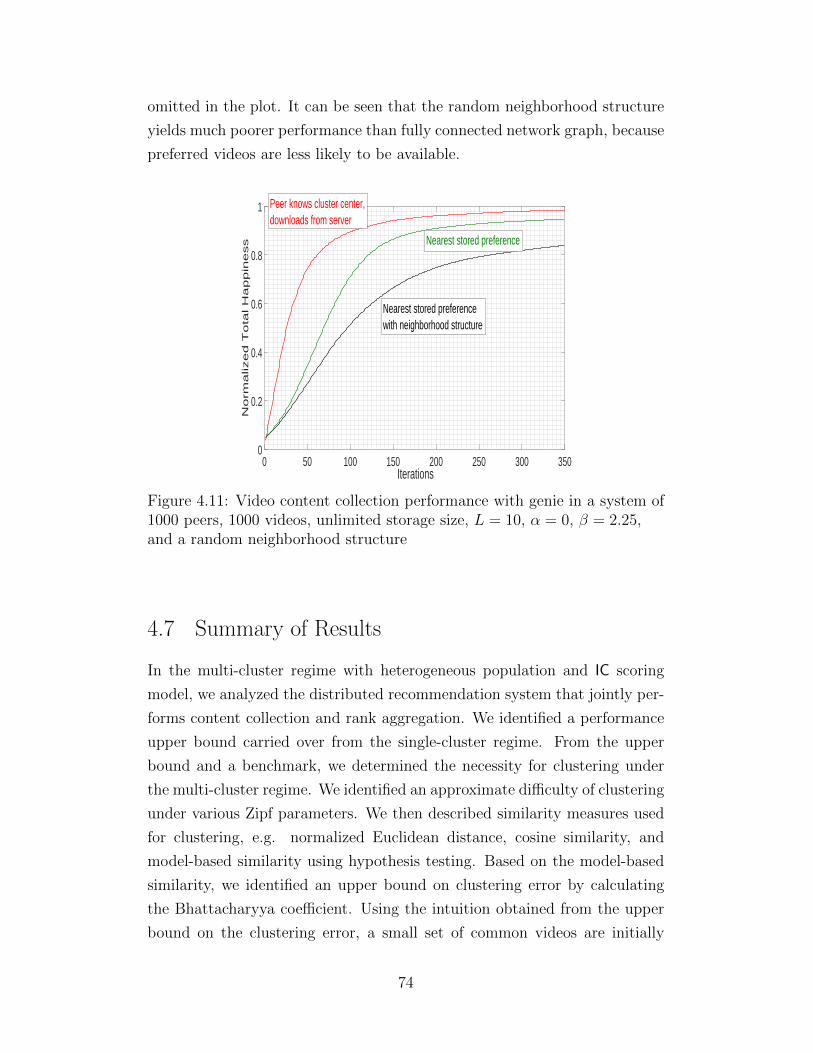
omitted in the plot. It can be seen that the random neighborhood structure

yields much poorer performance than fully connected network graph, because

preferred videos are less likely to be available.

Iterations0 50 100 150 200 250 300 350

No

rma

lize

d T

ota

l H

ap

pin

ess

0

0.2

0.4

0.6

0.8

1 Peer knows cluster center,downloads from server

Nearest stored preference

Nearest stored preferencewith neighborhood structure

Figure 4.11: Video content collection performance with genie in a system of1000 peers, 1000 videos, unlimited storage size, L = 10, α = 0, β = 2.25,and a random neighborhood structure

4.7 Summary of Results

In the multi-cluster regime with heterogeneous population and IC scoring

model, we analyzed the distributed recommendation system that jointly per-

forms content collection and rank aggregation. We identified a performance

upper bound carried over from the single-cluster regime. From the upper

bound and a benchmark, we determined the necessity for clustering under

the multi-cluster regime. We identified an approximate difficulty of clustering

under various Zipf parameters. We then described similarity measures used

for clustering, e.g. normalized Euclidean distance, cosine similarity, and

model-based similarity using hypothesis testing. Based on the model-based

similarity, we identified an upper bound on clustering error by calculating

the Bhattacharyya coefficient. Using the intuition obtained from the upper

bound on the clustering error, a small set of common videos are initially

74

given to each peer in order to increase the clustering accuracy.

Four multi-cluster aware recommendation rules were proposed. With some

modifications to the MLE rule, we proposed two deluxe recommendation

rules that estimate the cluster center scores: the Bayesian recommendation

rule with soft clustering and that with hard clustering. We proposed a

simple greedy recommendation rule inspired by the direct recommendation

rule, called the nearest stored preference rule. Lastly, we proposed a multi-

cluster aware global list recommendation rule that is modified from Cruz’s

recommendation rule. In terms of accumulation of information, peers under

the nearest stored preference rule and the Bayesian recommendation rules

need to store partial preference vectors, while the multi-cluster aware global

list recommendation rule does not. In terms of processing information, the

nearest stored preference rule has the simplest filtering algorithm.

A main conclusion is that distributed content collection and rank aggrega-

tion is feasible. Under well separated cluster centers, the proposed recommen-

dation rules all perform similarly, and the nearest stored preference rule is the

simplest. Under more correlated cluster centers, the nearest stored preference

rule works remarkably well, behaving similarly to the direct recommendation

rule in the single-cluster regime with homogeneous population. In general,

either exponential accumulation of partial preference vectors or neighbor

assignments such that neighbors have similar preferences is sufficient for the

nearest stored preference rule and Bayesian recommendation rules to achieve

near optimal performance.

75

CHAPTER 5

CONCLUSION

This thesis aims to understand a distributed system with joint content col-

lection and rank aggregation. For the single-cluster PL ranking model, we

presented a trivial performance upper bound and a tighter performance upper

bound using stochastic comparison. Using the intuition obtained from the

performance upper bound, we applied Hunter’s MM algorithm and proposed

an elaborate recommendation rule using this algorithm. We reevaluated

Cruz’s recommendation rule and proposed more efficient variations of the rule

that recursively combine partial rankings. Specifically, these are the linear

weighting functions. We also proposed a simple greedy recommendation

rule called direct recommendation and found in simulations that it is near

optimal. The direct recommendation rule is also robust in the sense that it

performs remarkably well over a broad range of system parameters.

For the single-cluster IC score model, we applied Kurtz’s theorem in the

fluid limit where the number of peers and number of videos go to infinity.

With several steps of simplification based on symmetry in the fluid limit and

the LLN, we were able to perform an exact asymptotic analysis of the direct

recommendation rule. We also stated a relationship between PL model and IC

model under the fluid limit. Using insights gained from this relationship, we

provided a simple explicit approximation formula for the performance of the

IC model under the direct recommendation rule. We also found in simulations

that the numerical performance result is very good approximation for the

direct recommendation rule under PL model in the fluid limit. In addition,

the numerical result of the direct recommendation rule appears to be near

optimal.

For the multi-cluster IC score model, we proposed four multi-cluster aware

recommendation rules based on the insights gained from the study of recom-

mendation rules under the single-cluster regime. We distinguished two as-

pects of a recommendation rule: accumulation of information and processing

76

of information. We extended the MLE recommendation rule from Hunter’s

MM algorithm to two recommendation rules: the Bayesian recommenda-

tion rule with soft clustering and that with hard clustering. The Bayesian

recommendation rules apply a complex filtering algorithm. We proposed a

simple greedy recommendation rule similar to the direct recommendation

rule, called the nearest stored preference rule, and found in simulations that

its performance is relatively good. The nearest stored preference rule applies

a simple filtering algorithm. Peers utilizing the nearest stored preference rule

or the Bayesian recommendation rules store multiple preference vectors up to

a storage constraint. We also extended the global list recommendation rule

by Cruz to a recommendation rule called the multi-cluster aware global list

recommendation rule. The multi-cluster aware global list recommendation

rule applies a complex filtering algorithm, but each peer recursively combines

partial preference vectors and stores only an aggregated version. However,

an aggregate of the partial preference vectors introduces noise in the multi-

cluster regime, so the performance of the multi-cluster aware global list

recommendation rule is not as good as the other recommendation rules when

peers in different clusters are correlated. Finally, for the accumulation of

preference information, we found that if the preferences of peers in different

clusters are nearly independent, either exponential accumulation of partial

preference vectors or neighbor assignments such that most neighbors have

similar preferences is sufficient for near optimal performance.

77

REFERENCES

[1] E. Candes and Y. Plan, “Matrix completion with noise,” IEEE, vol. 98,pp. 925–936, 2010.

[2] G. Bresler, G. Chen, and D. Shah, “A latent source model for onlinecollaborative filtering,” in Proc. NIPS, Montreal, Canada, 2014, pp.3347–3355.

[3] G. Bresler, D. Shah, and L. F. Voloch, “Collaborative filtering with lowregret,” 2015, arXiv:1507.05371 [cs.LG].

[4] O. Dabeer, “Adaptive collaborating filtering: The low noise regime,” inProc. ISIT, Istanbul, Turkey, 2013, pp. 1197–1201.

[5] G. Biau, B. Cadre, and L. Rouviere, “Statistical analysis of k-nearestneighbor collaborative recommendation,” The Annals of Statistics,vol. 38, pp. 1568–1592, 2010.

[6] L. Massoulie, M. Ohannessian, and A. Proutiere, “Greedy-Bayes ap-proach for targeted news dissemination,” in Proc. Sigmetrics, New York,NY, 2015, pp. 285–296.

[7] S. Caron and S. Bhagat, “Mixing bandits: A recipe for improved cold-start recommendations in a social network,” in Workshop on SocialNetwork Mining and Analysis, New York, NY, 2013.

[8] R. L. Cruz, “Ad-hoc networks at global scale,” in Proc. ICNC, SanDiego, CA, 2013, pp. 813–817.

[9] T. Qin, X. Geng, and T.-Y. Liu, “A new probabilistic model forrank aggregation,” in Proc. Advances in Neural Information ProcessingSystems 23, Vancouver, Canada, 2010, pp. 1948–1956.

[10] J. A. Lozano and E. Iruozki, “Probabilistic modeling on rankings,”2012. [Online]. Available: http://www.sc.ehu.es/ccwbayes/members/ekhine/tutorial ranking/data/slides.pdf

[11] S. Jagabathula and D. Shah, “Inferring rankings under constrainedsensing,” in Proc. NIPS, Vancouver, Canada, 2008, pp. 753–760.

78

[12] M. Braverman and E. Mossel, “Sorting from noisy information,” 2009,arXiv:0910.1191 [cs.DS].

[13] R. Plackett, “The analysis of permutations,” Applied Statistics, vol. 24,pp. 193–202, 1975.

[14] R. D. Luce, Individual Choice Behavior: A Theoretical Analysis. NewYork: Wiley, 1959.

[15] R. A. Bradley and M. E. Terry, “Rank analysis of incomplete blockdesigns i: The method of paired comparisons,” Biometrika, vol. 39, pp.324–345, 1952.

[16] D. R. Hunter, “MM algorithms for generalized Bradley-Terry models,”The Annals of Statistics, vol. 32, pp. 384–406, 2004.

[17] J. Guiver and E. Snelson, “Bayesian inference for Plackett-Luce rankingmodels,” in Proc. International Conference on Machine Learning, NewYork, NY, 2000, pp. 753–760.

[18] T. Minka, “Divergence measures and message passing,” MicrosoftResearch, Technical Report, 2005.

[19] Z. Cao, T. Qin, T. Y. Liu, M. F. Tsai, and H. Li, “Learning torank: From pairwise approach to listwise approach,” Microsoft Research,Technical Report, 2007.

[20] L. Thurstone, “A law of comparative judgement,” Psychological Reviews,vol. 34, pp. 273–286, 1927.

[21] J. Yellott, “The relationship between Luce’s choice axiom, Thurstone’stheory of comparative judgement, and the double exponential distribu-tion,” Journal of Mathematical Psychology, vol. 15, pp. 109–144, 1977.

[22] S. Boyd, A. Ghosh, B. Prabhakar, and D. Shah, “Randomized gossipalgorithms,” Journal IEEE/ACM Transactions on Networking, vol. 14,pp. 2508–2530, 2006.

[23] A. Nedich, Convergence Rate of Distributed Averaging Dynamics andOptimization in Networks. Now Publishers, 2015, vol. 2.

[24] L. A. Adamic, “Zipf, power-laws, and Pareto - a ranking tutorial,” http://www.hpl.hp.com/research/idl/papers/ranking/ranking.html, 2002.

[25] A. Dempster, N. Laird, and B. Rubin, “Maximum likelihood fromincomplete data via the EM algorithm,” Royal Statistical Society,vol. 39, pp. 1–38, 2006.

79

[26] P. S. Efraimidis and P. G. Spirakis, “Weighted random sampling with areservoir,” Information Processing Letters, vol. 97, pp. 181–185, 2006.

[27] J.-Y. L. Boudec, D. McDonald, and J. Mundinger, “A generic meanfield convergence result for systems of interacting objects,” in Proc.Quantitative Evaluation of Systems. IEEE, 2007, pp. 3–18.

[28] R. Darling and J. Norris, “Differential equation approximations forMarkov chains,” Probability Surveys, vol. 5, pp. 37–79, 2008.

[29] W. Hoeffding, “Probability inequalities for sums of bounded randomvariables,” Journal of the American Statistical Association, vol. 58, no.301, pp. 13–30, 1963.

[30] M. Mitzenmacher and E. Upfal, Probability and Computing: RandomizedAlgorithms and Probabilistic Analysis. New York, NY, USA: CambridgeUniversity Press, 2005.

[31] S. Ethier and T. Kurtz, Markov Processes: Characterization andConvergence. Wiley, 2009, vol. 282.

[32] V. Poor, An Introduction to Signal Detection and Estimation. Springer,1998.

80