Embed Size (px)
Citation preview

UCGE Reports Number 20294
Department of Geomatics Engineering
Development of Laser Fluorosensor Data Processing System and GIS Tools for Oil Spill Response
(URL: http://www.geomatics.ucalgary.ca/research/publications)
by
Maya Nand Jha
September 2009
UNIVERSITY OF CALGARY
Development of Laser Fluorosensor Data Processing System and GIS Tools for Oil Spill
Response
by
Maya Nand Jha
A THESIS
SUBMITTED TO THE FACULTY OF GRADUATE STUDIES
IN PARTIAL FULFILMENT OF THE REQUIREMENTS FOR THE
DEGREE OF (MASTER OF SCIENCE)
DEPARTMENT OF GEOMATICS ENGINEERING
CALGARY, ALBERTA
September, 2009
© Maya Nand Jha (2009)
ii
Abstract
An oil spill detection and decision support system is a critical tool in protecting
oceanic environment and reducing economic losses due to oil spill. Remote sensing data
can help in detecting minor spills before they cause widespread damage. This thesis
examines the characteristics and applications of different sensors with regard to oil spill
surveillance. Laser Fluorosensors, such as the Scanning Laser Environmental Airborne
Fluorosensor (SLEAF) sensor operated by Environment Canada, are among the most
appropriate sensors for oil spill surveillance. Algorithms for detecting oil spills using
laser fluorosensor datasets are analyzed. The algorithms are compared on the basis of
their ability to identify oil in the Scanning Laser Environmental Airborne Fluorosensor
(SLEAF) data as well as from the simulated data. A classification scheme is developed
for oil spill detection and classification based on the analysis. The developed oil spill
detection and classification scheme is employed to detect and classify oil from SLEAF
data acquired in parts of west and east coast of Canada.
Though various components and software tools exist for managing specific tasks
involved in oil spill response, there is a need to develop a comprehensive integrated
system for oil spill response. An integrated oil spill detection and response system can
greatly help disaster managers in directing resources and equipments for oil spill cleaning
and containment operations to appropriate locations. A software system is developed to
exhibit the feasibility of realizing such an integrated oil spill detection and decision
support system. The oil spill trajectory modeling tool is developed as a part of the system.
iii
Acknowledgements
This thesis is based on extensive research for around two years. This thesis would
not have been possible without support from many people. First, I would like to thank my
supervisor Dr. Yang Gao for his constant support, guidance and encouragement
throughout my research. I sincerely thank ESTD, Environment Canada and particularly
Dr. Brown for kindly providing the SLEAF dataset for this thesis. I wish to express my
deep appreciation to Dr. Xin Wang, Dr. Ayman Habib and Dr. Ron Wong for carefully
reading and providing comments concerning various aspects of this research.
I have been far from my parents Dr. Baua Nand Jha and Indira Jha during this
research but I always felt the warmth of their affection with me. I would like to thank my
brother Jaya Nand Jha and my sister-in-law Rashmi Jha for their constant encouragement
and support. I am grateful to my sister Hema Jha and brother-in-law Dr. Mani Kumar for
their love and support.
Members of PMIS research group have been really helpful and I am thankful to
them. I am grateful to members of DPRG group for their friendliness. I want to
particularly thank Ki In Bang for giving valuable suggestions in geo-referencing SLEAF
data, and Anna Jarvis for help and emotional support. The stay at University of Calgary
would not have been so much fun without my friends Sneha and Nidhi. Last but not the
least, I appreciate help and support from my flat-mates Jaydeep Tailor and Sandeep
Chandana during this research.

iv
Dedication
To my mother “Indira Jha” whose categorical love, affection
and occasional chiding has given me strength and guided me throughout
the life.
v
Table of Contents
Approval Page ..................................................................................................................... ii
Abstract ............................................................................................................................... ii
Acknowledgements ............................................................................................................ iii
Dedication .......................................................................................................................... iv
Table of Contents .................................................................................................................v
List of Tables .................................................................................................................... vii
List of Figures and Illustrations ....................................................................................... viii
List of Symbols, Abbreviations and Nomenclature ........................................................... xi
CHAPTER ONE: INTRODUCTION ..................................................................................1
1.1 Damages Caused by Oil Spill ....................................................................................1
1.2 Oil Spill Surveillance .................................................................................................3
1.3 Oil Spill Trajectory Modeling ....................................................................................5
1.4 Oil Spill Response and GIS .......................................................................................8
1.5 Research Objectives .................................................................................................11
1.6 Thesis Outline ..........................................................................................................12
CHAPTER TWO: STATE-OF-THE-ART SENSORS TECHNOLOGY FOR OIL
SPILL SURVEILLANCE .........................................................................................13
2.1 Remote Sensing for Oil Spill Surveillance ..............................................................13
2.1.1 Visible Sensors ................................................................................................14
2.1.2 Infrared Sensors ...............................................................................................16
2.1.3 Ultraviolet Sensors ..........................................................................................16
2.1.4 Radar ................................................................................................................17
2.1.5 Microwave .......................................................................................................19
2.1.6 Laser fluorosensor ...........................................................................................19
2.1.7 Laser-acoustic oil thickness sensor .................................................................21
2.2 Comparison of Remote Sensing Systems for Oil Spill Surveillance .......................22
CHAPTER THREE: EXISTING METHODS FOR LASER FLUOROSENSOR
DATA PROCESSING ..............................................................................................28
3.1 Oil Spill Detection using Laser Fluorosensors ........................................................28
3.2 Oil Spill Detection Methods and Algorithms ..........................................................37
CHAPTER FOUR: A SCHEME FOR OIL SPILL DETECTION AND
TRAJECTORY MODELING ...................................................................................40
4.1 Description of Dataset .............................................................................................40
4.2 Comparative Evaluation of Existing Methods for Oil Spill Detection ....................41
4.3 A Proposed Oil Spill Detection and Classification Scheme ....................................53
4.4 Geo-referencing of SLEAF Data .............................................................................58
4.5 Oil Spill Trajectory Modeling using Cellular Automata .........................................67
CHAPTER FIVE: RESULTS AND DISCUSSION ..........................................................71
5.1 Results of using Proposed Scheme on SLEAF Data ...............................................72
5.2 Oil Spill Disaster Products .......................................................................................76
vi
CHAPTER SIX: DEVELOPMENT OF A TOOL FOR OIL SPILL DETECTION
AND RESPONSE .....................................................................................................84
6.1 System Architecture .................................................................................................84
6.2 Software Tool Development ....................................................................................89
CHAPTER SEVEN: CONCLUSIONS AND RECOMMENDATIONS ..........................99
7.1 Conclusions ..............................................................................................................99
7.2 Recommendations ..................................................................................................101
REFERENCES ................................................................................................................103

vii
List of Tables
Table 1.1: Appearance of Oil on a Calm Water Surface .................................................... 3
Table 2.1: Remote Sensing Bands and Related Instruments used for Oil Spill
Detection (Adapted from Goodman, 1994) .............................................................. 14
Table 2.2: Requirements for Oil Spill Detection (Adapted from Fingas et al., 1998) ...... 23
Table 2.3: Comparison of Various Sensors for Oil Spill Detection ................................. 26
Table 3.1: Technical Specifications for some Laser Fluorosensors ................................. 30
Table 4.1: Summary Statistics for Light Oils (Data Source: Environment Canada) ........ 42
Table 4.2: Summary Statistics for Heavy Oils (Data Source: Environment Canada) ...... 43
Table 4.3: Summary Statistics for Some Crude Oils (Data Source: Environment
Canada) ..................................................................................................................... 43
Table 4.4: Summary Statistics for Background Materials (Data Source: Environment
Canada) ..................................................................................................................... 44
Table 4.5: Classification Results using Various Algorithms for Simulated Data............. 53
Table 4.6: Typical Values of Thresholds for Oil Spill Detection and Classification
Scheme ...................................................................................................................... 56

viii
List of Figures and Illustrations
Figure 1.1: Sea Birds Affected by the Exxon Valdez Oil Spill (Photo Courtesy of the
Exxon Valdez Oil Spill Trustee Council) ................................................................... 2
Figure 1.2: Processes Involved In Determining Fate and Behaviour of Oil Spill
(Graph Courtesy Of ITOP. © International Tanker Owners Pollution Federation
Limited (ITOPF ) ........................................................................................................ 7
Figure 2.1: Image of Exxon Valdez Oil Spill Captured by a Sensor in the Visible
Range (Source: NOAA, 2007) .................................................................................. 15
Figure 2.2: SAR Image (RADARSAT-1) of Oil Spill Caused by Katrina Hurricane
(2005) in the Gulf of Mexico .................................................................................... 18
Figure 2.3: Schematic Diagram of the Laser Fluorosensor (source: Laser Diagnostic
Instruments AS (LDI)) .............................................................................................. 20
Figure 3.1: Fluorescence Spectra of Light Oils. Data Source: Environment Canada ....... 31
Figure 3.2 Fluorescence Spectra of Crude Oils (Data Source: Environment Canada) ..... 32
Figure 3.3: Fluorescence Spectra of Heavy Oils (Data Source: Environment Canada) ... 32
Figure 3.4: Fluorescence Spectra of Background Materials (Data Source:
Environment Canada) ............................................................................................... 33
Figure 3.5: Fluorescence Spectra of Natural Water for Excitation Wavelength as 308
nm (Adapted from Grüner, 1991) ............................................................................ 34
Figure 3.6: Laser Induced Fluorescence (LIF) spectrum for Oil Slick and Sea Water
(Adapted from Hoge and Swift, 1980) ..................................................................... 35
Figure 4.1: Sample Simulated Data Generated for Light Oil by adding 10% Gaussian
Noise ......................................................................................................................... 45
Figure 4.2: Eigenvalues for the PCs Computed for Reference Spectrum......................... 49
Figure 4.3: PC Loading for Reference Materials .............................................................. 50
Figure 4.4: 3D Scatter Plot of Reference Materials in the PC Space ............................... 50
Figure 4.5: 2D Scatter Plot of Reference Materials in the PC Space (PC1 and PC2) ...... 51
Figure 4.6: Eigenvalues for the PCs Computed for Ratio Components ........................... 51
Figure 4.7: 3D Scatter Plot of Reference Materials in the PC Space for Ratio
Components .............................................................................................................. 52

ix
: Figure 4.8: Correlation Map for Reference Fluorescence Spectra ................................. 56
Figure 4.9: Scheme for Oil Spill Detection and Classification ......................................... 57
Figure 4.10: Components and Coordinate Systems for a Typical LiDAR System .......... 60
Figure 4.11: Coordinate Systems for SLEAF ................................................................... 61
Figure 4.12: Angular Field of Views for Elliptical Scanner ............................................. 64
Figure 4.13: Angular Position of a Point in Elliptical Footprint ....................................... 65
Figure 4.14: The Von Neumann Neighborhood ............................................................... 67
Figure 4.15: The Moore Neighborhood ............................................................................ 67
Figure 4.16: Oil Masses in Neighbourhood of Cell (i,j) at Time t.................................... 68
Figure 5.1: Study Area Displaying Locations of SLEAF Test Flights Conducted by
Environment Canada ................................................................................................. 72
Figure 5.2: Observed Fluorescence Spectra for Thick Oil Film of Diesel in Vancouver
Island ......................................................................................................................... 74
Figure 5.3: Observed Fluorescence Spectra for Thin Film of .......................................... 74
Diesel in Vancouver Island Area ...................................................................................... 74
Figure 5.4: Fluorescence Spectra of Water (Gelbstoff) in Vancouver Island Area .......... 75
Figure 5.5: Fluorescence Spectra of Turbid Water in Vancouver Island Area ................. 75
Figure 5.6: Fluorescence Spectra of Water (Gelbstoff) in East Coast of Canada ............. 76
Figure 5.7: Georeferenced and Processed SLEAF Data in East Coast of Canada ........... 79
Figure 5.8: Oil Spill Detected around Vancouver Island .................................................. 79
Figure 5.9: Oil Slick Extracted from SLEAF Data around Vancouver Island ................. 80
Figure 5.10: Emergency Response Map for Oil Spill at Vancouver Island...................... 81
Figure 5.11: Oil Spill Trajectory Map with Assumed Parameters for Trajectory
Modeling ................................................................................................................... 82
Figure 5.12: ESI map for the Shoreline of Southern California (Source: NOAA) ........... 83
Figure 6.1: Use Case Scenerio for Integrated System for Oil Spill Response ................. 88

x
Figure 6.2: System Architecture of Integrated System for Oil Spill Response ............... 88
Figure 6.3: SLEAF Data Processing and Analysis Flow Chart ........................................ 91
Figure 6.4: Hawth’s Analysis Tool for Creating Vector Grids ......................................... 92
Figure 6.5: Software Tool Providing General Information about the Prototype System . 93
Figure 6.6: Laser Fluorosensor Data Processing Part of the System ................................ 93
Figure 6.7: Dialog Box Showing that Processing of Laser Fluorosensor Data is
Complete ................................................................................................................... 94
Figure 6.8: Tool for Oil Spill Incident Reporting ............................................................. 94
Figure 6.9: Oil Spill Trajectory Modeling Tool Showing Options for Selecting
Different Oil Types ................................................................................................... 95
Figure 6.10: Oil Spill Trajectory Modeling Tool Showing Options for Selecting
Different Measurement Type for Oil ........................................................................ 95
Figure 6.12: Trajectory of Oil Spill after Time Interval of 150 Minutes .......................... 96
Figure 6.13: GUI for GIS Analysis Component of the System ........................................ 97
Figure 6.14: Oil Spill Emergency Response Map Displayed in GIS Analysis Tool ........ 97
Figure 6.15: Oil Spill Trajectory Map Displayed in GIS Analysis Tool .......................... 98
Figure 6.16: ESI Map Displayed in GIS Analysis Tool ................................................... 98

xi
List of Symbols, Abbreviations and Nomenclature
Abbreviation Definition AISA Airborne Imaging Spectrometer for
Applications
APIs Application Programming Interfaces
AVIRIS Airborne Visible/Infrared Imaging
Spectrometer
CA Cellular Automaton
CAs Cellular Automata
CDOM Coloured Dissolved Organic Matter
DSS Decision Support System
EMS Enterprise Message Service
ENEA Ente per le Nuove tecnologie, l'Energia e
l'Ambiente
ESB Enterprise Service Bus
ESI Environmental Sensitivity Index
ESRI Environmental Systems Research Inc.
ESTD Emergency Science and Technology Division
GIS Geographic Information Systems
GNOME General NOAA Operational Modeling
Environment
GNSS Global Navigation Satellite System
GPS Global Positioning System
GUI Graphical User Interface
IDE Integrated Development Environment
INS Inertial Navigation System
IR Infrared
IROE-CNR Istituto di Ricerca sulle Onde
Elettromagnetiche del Consiglio Nazionale
delle Richerche
ISTOP Integrated Satellite Tracking of Oil polluters
LBS Location Based Services
LDI Laser Diagnostic Instruments
LEAF Laser Environmental Airborne Fluorosensor
LiDAR Light Detection and Ranging
LIF Laser Induced Fluorescence
LURSOT Laser-Ultrasonic Remote Sensing of Oil
Thickness
MIR Mid-band Infrared
MWR Microwave radiometer
NOAA National Oceanic and Atmospheric
Administration
PMIS Positioning and Mobile Information Systems
PCA Principal Component Analysis
PCs Principal Components
xii
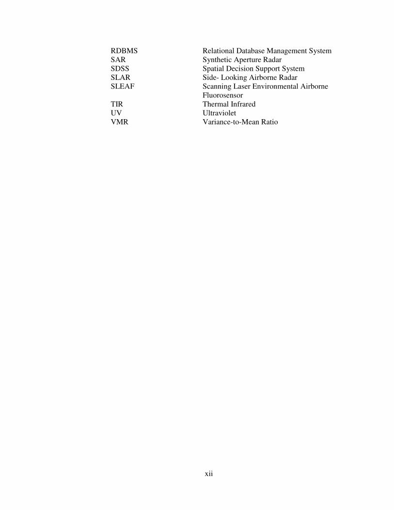
RDBMS Relational Database Management System
SAR Synthetic Aperture Radar
SDSS Spatial Decision Support System
SLAR Side- Looking Airborne Radar
SLEAF Scanning Laser Environmental Airborne
Fluorosensor
TIR Thermal Infrared
UV Ultraviolet
VMR Variance-to-Mean Ratio

1
Chapter One: Introduction
Petroleum products play an important role in modern society, particularly in the
transportation, plastics, and fertilizer industries. There are typically ten to fifteen transfers
involved in moving oil from the oil field to the final consumer. Oil spills can occur
during the transportation or storage of the oil, and the spillage can happen in water, ice or
on land. Marine oil spills can be highly dangerous given that the wind, waves and
currents can scatter an oil spill over a wide area within just a few hours in the open sea
(Fingas, 2001). Between 1988 and 2000, there were 2,475 spills which released over
800,000 litres of oil in Toronto and surrounding regions (Li, 2002). An oil spill can
occur due to a number of reasons, including transportation accidents. Grüner (1991)
mentions that in addition to accidents, the controlled release of oil by shipping operators
and oil production platforms are major sources of oil spill. Many oiled birds have been
found in the east and west coast of Canada due to illegal oil discharges (Brown et al.,
2004a and Brown et al., 2006b). Various measures such as firm legislations and strict
operating procedures have been imposed to prevent oil spills, but these measures cannot
completely eliminate the risk of oil spills (Fingas, 2001).
1.1 Damages Caused by Oil Spill
Once oil is spilled, it quickly spreads to form a thin layer on the water surface,
known as an “oil slick”. As time passes, the oil slick becomes thinner, forming a layer
known as “sheen” which has a rainbow like appearance. Light oils are highly toxic but
evaporate quickly. Heavy oils are less toxic but persist in the environment for a long
time. Heavy oils can get mixed with pebbles and sandy beaches and remain there for
years (Environment Canada, 2007). Fuels and crude oil contribute to 48% and 29% of

2
total spilled oil into the sea worldwide, respectively (Brekke and Solberg, 2005). The
environmental impacts of oil spills can be considerable. Oil spills in water may severely
affect the marine environment causing a decline in phytoplankton and other aquatic
organisms. Phytoplankton is at the bottom of the food chain and can pass absorbed oil on
to higher levels in the food chain. Oiled birds display behavioural changes leading to loss
of eggs and even death (Figure 1.1). The livelihood of many coastal people can be
impacted by oil spills, particularly those whose livelihood is based on fishing and tourism
(NOAA, 2009). The movement of oil on land depends on various factors such as oil type,
soil type and moisture content of the soil. Oil spilled on agricultural land can impact soil
fertility and pollute ground water resources (Fingas, 2001).
Figure 1.1: Sea Birds Affected by the Exxon Valdez Oil Spill (Photo Courtesy of the Exxon Valdez Oil Spill Trustee Council)

3
1.2 Oil Spill Surveillance
Oil spill surveillance constitutes an important component of oil spill disaster
management. Advances in remote sensing technologies can help to identify parties
potentially responsible for oil spill incident and to identify minor spills before they cause
widespread damage (Jha et al., 2008a). Remote sensing data can be very useful input for
an oil spill detection and decision support system (DSS). Fingas (2001) describes the
guidelines for estimating oil thickness using visual surveillance as shown in Table 1.1.
The appearance of oil varies from silvery-sheen to dark brown.
Table 1.1: Appearance of Oil on a Calm Water Surface
Oil Appearance Approximate Film
Thickness (µµµµm)
Silvery sheen 0.05
Rainbow sheen 0.15
Reddish-brown sheen 0.50
Brownish 2.00
Dark 10.00
Dark Brown 50.00
Visual detection of an oil spill is not reliable as oil can be confused with other
substances, e.g. sea weeds and fish sperm. Moreover, oil on the surface cannot be
observed clearly through fog and darkness (Fingas, 2001). Remote sensing can be used

4
for detecting and monitoring oil spills. Sensors can provide the following information for
oil spill contingency planning (Grüner, 1991):
• The location and spread of an oil spill over a large area
• The thickness distribution of an oil spill to estimate the quantity of spilled
oil
• A classification of the oil type in order to estimate environmental damage
and to take appropriate response activities
• Timely and valuable information to assist in clean-up operations
Remote sensing technologies for oil spill surveillance have been reviewed by
many authors. Goodman (1994) notes that the operational use of remote sensing for oil
spill contingency planning is limited although simple systems, such as UV/IR systems
and radar, have been used to some extent for responding to oil spills. Brown and Fingas
(1997) found that no single sensor can give all the information required for oil spill
contingency planning. Currently, many coastal nations have proper maritime surveillance
systems in place to detect and monitor oil spill (Brown and Fingas, 2005). Due to the
large number of sensors currently available for oil spill surveillance, there is a need for a
comprehensive overview and comparison of the existing sensors. A better understanding
of the oil spill surveillance sensor characteristics will help improve the effectiveness and
operational use of these sensors for oil spill response and contingency planning. Laser
Fluorosensors can detect oil under the water surface and on various backgrounds
including snow or ice (Brown and Fingas, 2003a). The operational use of laser
fluorosensors is expected to increase with time since it is the most useful instrument for
oil spill detection (Jha et al., 2008b). Accordingly, it is important to analyze the reliability

5
and robustness of various oil spill detection algorithms. In this thesis, an in-depth analysis
of existing algorithms for oil spill detection and classification is provided, further to
which, a novel method is developed.
1.3 Oil Spill Trajectory Modeling
Once oil is spilled in an oceanic environment, it is important to know the
movement of oil spill from the start of the incident to its removal from the sea due to
various processes. Moreover, the knowledge about the oil state such as density, viscosity,
emulsion state and chemical composition is also needed at all stages of oil spill for
choosing the appropriate response actions. Oil spill modeling in the oceanic environment
is a complicated process as the behaviour and spread of the spilled oil depends on various
processes including evaporation, drift, spreading, emulsification, dispersion, dissolution
and entrainment (Figure 1.2). These processes are described briefly here.
• Drift: Drift is the horizontal and vertical transport of centre of the oil slick
by wind and sea currents.
• Spreading: The oil slick area increases and oil slick thickness decreases
with time in the spreading process. Spreading is an important aspect in
understanding its role in the weathering process and containment
operations.
• Natural dispersion: Dispersion is the process by which wind-driven
waves split the surface oil layer into water droplets and propel them into
the water column.
• Emulsification: Water comes into the oil and forms water-in-oil
emulsions. The main effect of emulsification is the increase in the
6
viscosity and the volume of the oil spill. This makes clean up operations
more difficult.
• Evaporation: The volatile components in the oil go from their liquid state
into vapours. Light oil evaporates quicker than heavy oils. Evaporation
can cause loss of petroleum hydrocarbons upto 25% in short term and 40%
in the long term.
• Dissolution: Dissolution is the process in which the soluble components
of crude oil dissolve into water. It is more active when spill first occurs.
• Sedimentation and shoreline stranding: Sedimentation is the process
when spilled oil reaches a coastline and returns to the marine environment
• Photo-oxidation: Oil undergoes oxidation in presence of sunlight. This is
a long term process.
• Biochemical degradation: Micro-organisms break petroleum
hydrocarbons into simpler products. Biochemical degradation is also a
long term process.

7
Figure 1.2: Processes Involved In Determining Fate and Behaviour of Oil Spill (Graph Courtesy Of ITOP. © International Tanker Owners Pollution Federation Limited (ITOPF )
A detailed analysis of the current techniques available for oil spill modeling can
be found in Reed et al. (1999), Brebbia (2001) and Fingas (2001). Cellular Automata
(CAs) are simple but useful technique to model complicated physical processes in
discrete space and time. It was introduced by Ulam and Von Neumann in 1951. Fate of
oil spill in oceanic environment can be successfully modeled using cellular automata
(Karafyllidis, 1997; Rusinovic and Bogunovic, 2006). Karafyllidis (1997) has proposed a
simple method to model oil spill trajectory using CAs which has been applied in this
thesis to develop a tool for oil spill trajectory modeling. The details of the method
developed by Karafyllidis (1997) for oil spill trajectory modeling using Cellular
Automata is provided in section 4.5.

8
1.4 Oil Spill Response and GIS
Contingency planning refers to establishing some plan of action to counter
emergencies. The purpose of contingency planning is to minimize economic and
environmental damages in case of an oil spill. Fingas (2001) has described that response
action for an oil spill can be divided into various phases such as alerting and reporting,
evaluation and mobilization, containment and recovery, disposal and remediation.
However, traditional methods suffer from the lack of updated information and situational
awareness. Hugh (1977) developed an oil spill contingency plan for oil spill response in
marine environment. His plan emphasized on resources at risk such as aquatic organisms
and public beaches. Green (1996) notes that effective response planning should include
timely acquisition of data and information in a cost-effective manner. Geographic
information systems (GIS) with comprehensive storage and analysis capability can be an
effective tool for oil spill response (Howlett and Bradstreet, 1996). Moreover, GIS is
designed to solve spatial problems and many issues related to oil spill contingency
planning and any emergency management are spatial.
The response time is crucial for an oil spill in the open ocean as wind and current
can rapidly spread the oil over a large area in a short time. GIS can facilitate rapid
response and thereby mitigate environmental and economic damages caused by an oil
spill. The timeframe for collecting and processing the data is important for oil spill
surveillance and monitoring. Real time remote sensing data is essential for oil spill
response so that resources can be immediately directed to sensitive areas for cleaning and
containment operations. The integration of a remote sensing data processing component
with GIS can greatly assist decision makers. Environmental sensitivity index (ESI)

9
describes the susceptibility of shorelines due to damages caused by oil pollution (Fingas,
2001). ESI is commonly used for evaluating potential risks due to an oil spill. ESI map as
a GIS tool can be useful for oil spill decision support system. In addition to having
shorelines ranked in terms of their susceptibility to damage caused by an oil spill, it also
includes the areas which are environmentally or economically sensitive to an oil spill.
ESI map has information about location of fishes, birds, human facilities, any relevant
natural feature, types of shoreline etc. ESI maps for USA shorelines are freely available
at National Oceanic and Atmospheric Administration (NOAA) website which can be
combined with oil spill models to predict the impact of an oil spill. ESI maps for Canada
are maintained by oil spill responding agencies, but are not freely available for public
use. The list of agencies that need to be notified about an oil spill should be part of any
oil spill contingency plan. There should also be a procedure to inform the public about
the oil spill incident. A GIS system can contain a list of individuals and agencies who
need to be notified in case of an oil spill, and they can be automatically notified in event
of an oil spill. Oil spill emergency response typically utilizes an extensive set of
resources, equipment and multiple agencies and the coordination between them is a
difficult and complex task. Effective communication is crucial to any emergency
response (Cova, 1999). A GIS based oil spill detection and decision support system can
facilitate communication between various agencies and any relevant data about oil spill
incident can be shared quickly among them.
A knowledge-based spatial decision support system (SDSS) for oil spill response
can resolve the problems ingrained in the traditional oil spill response decision making.
GIS is still mostly used as a spatial database or mapping tool for the oil spill response
10
(Ranger and Cassas, 1995). The problem is attributed to the lack of modeling capability
in the GIS system. Armstrong and Densham (1990) have mentioned that a spatial
decision support system (SDSS) consists of the following components:
1. A database management system
2. Analysis routines
3. Display and report generators
4. A user interface
There is a need for an oil spill decision support system, which can use available data and
information to tackle oil spill response in a better way. There are components available
for the various parts of oil spill response but an integrated comprehensive GIS system is
required to quickly respond to an oil spill. For example, General NOAA Operational
Modeling Environment (GNOME) is the oil spill trajectory model used by oil spill
responders in event of an oil spill but the environmental risk associated with an oil spill
can not be estimated using GNOME. The available expert knowledge can be put together
to build an expert system with GIS capabilities. A combination of GIS and an expert
system can provide significant advantages to decision makers. The unavailability of an
expert system for oil spill contingency planning despite significant advancement in
technologies acts as a hindrance in effective oil spill response (Graham, 2004; Ornitz and
Champ, 2002). A web-based GIS system can resolve the problem of accessibility. The oil
spill responders and responsible agencies can access the up-to-date information about an
oil spill from anywhere in the world if an internet connection is accessible.

11
1.5 Research Objectives
The primary objective of this research is to develop a scheme for oil spill
detection and classification. Laser fluorosensor data processing will be discussed in detail
due to the ability of laser fluorosensors in detecting and classifying oil on various
backgrounds in real time. This research also aims to develop additional tools including oil
spill trajectory modeling tool and oil spill disaster products which can help personnel
involved in oil spill response in taking quick and better decisions. The research objectives
of the thesis are:
• To evaluate various remote sensing sensors for oil spill detection and
classification. State-of-the-art sensors technology for oil spill surveillance will be
discussed and various sensors will be studied based on their ability to detect and
classify oil.
• To analyze issues associated with processing laser fluorosensor data for oil spill
detection and classification. The algorithms to process laser fluorosensor data will
be discussed and analyzed.
• To develop a scheme for oil spill detection and classification using laser
fluorosensor data. Reliable oil spill detection is important for oil spill response.
• To develop software which can act as an integrated system for oil spill response
and will include components for oil spill detection, oil spill trajectory modeling
and oil spill disaster products. System architecture for conceiving a GIS system
for oil spill response will be discussed. The developed software will demonstrate
that a system can be realized which can handle requirements of oil spill disaster
management.
12
1.6 Thesis Outline
Chapter 1 presents introduction, the problem statement and research objectives for
this thesis.
Chapter 2 contains review of the state-of-the-art sensors technology for oil spill
surveillance. Various remote sensing sensors available for oil spill surveillance are
discussed and compared based on several criteria.
Chapter 3 discusses the issues associated with processing laser fluorosensor data.
The advantages and disadvantages of various existing algorithms for laser fluorosensor
data are discussed.
Chapter 4 explains the oil spill detection and classification scheme that has been
developed in this research. Scanning Laser Environmental Airborne Fluorosensor
(SLEAF) data format is described. The procedure of geo-referencing SLEAF data is
explained as well. The use of Cellular Automata (CAs) for oil spill trajectory modeling is
described.
Chapter 5 provides the analysis of real world laser fluorosensor data based on oil
spill detection and classification scheme developed in this research. Oil spill disaster
products are discussed.
Chapter 6 explains development of a software tool for oil spill detection and
response. The system architecture for realizing an integrated system for oil spill response
is discussed. The technologies used for developing the software tool are explained in
detail.
Chapter 7 builds on the observations and conclusions drawn from this research as
well as recommendations for the future work.
13
Chapter Two: State-of-the-Art Sensors Technology for Oil Spill Surveillance
There are many sensors available to detect oil spills on various kinds of surfaces.
Oil spill location, extent as well as thickness distribution can be obtained by using remote
sensors. Multi-temporal imaging captured by remote sensing sensors can provide
important information required to model the spread of an oil spill (Natural Resources
Canada, 2009). Oil spill models may be useful for cleanup operations and controlling the
oil spill. Remote sensing devices for oil spill detection include infrared video and
photography, thermal infrared imaging, airborne laser fluorosensors, airborne and space-
borne optical sensors, and airborne and space-borne SAR (Natural Resources Canada,
2009). Satellite remote sensing suffers from low spatial and temporal resolution although
it provides a synoptic view and a more cost effective system than an airborne platform,
which is typically used for oil spill surveillance (Brown and Fingas, 2001a). The
usefulness of various sensors with regard to oil spill surveillance is described in this
chapter.
2.1 Remote Sensing for Oil Spill Surveillance
Remote sensing bands and related instruments for oil spill detection are shown in
Table 2.1. Infrared, visible and UV sensors will not be able to detect oil in inclement
weather such as heavy rain or fog (Goodman, 1994). Visible sensors are generally used to
create a base map for the oil spill. Active sensors use their own energy source to capture
information whereas passive sensors do not have their own energy source and rely on
other energy sources. A brief description of sensors useful for oil spill detection is given
in the following sections.

14
Table 2.1: Remote Sensing Bands and Related Instruments used for Oil Spill Detection (Adapted from Goodman, 1994)
Band Wavelength Type of Instruments
Radar 1-30 cm SLAR/SAR
Passive microwave 2-8 mm Radiometers
Thermal infrared (TIR) 8-14 µm Video cameras and line scanners
Mid-band infrared (MIR) 3-5 µm Video cameras and line scanners
Near infrared 1-3 µm Film and video cameras
Visual 350-750 nm Film, video cameras and
spectrometers
Ultraviolet 250-350 nm Film, Video cameras and line
scanners
2.1.1 Visible Sensors
Thermal and visible scanning systems as well as aerial photography were
commonly used airborne remote sensing sensors at the start of 1970 (Wadsworth, 1992).
Visible sensors (passive sensors operating in the visible region of the light) are still
widely used in oil spill remote sensing despite many shortcomings. The reflectance of oil
is higher than that of water but oil also absorbs some radiation in the visible region.
These sensors are not good for oil detection as it is difficult to distinguish oil from the
background (Figure 2.1). Water surface may have shining effect due to the blowing wind.
Sun-glint and wind sheen may create an impression similar to oil sheen. Moreover, sea
weeds and a darker shoreline may be mistaken for oil. Visible sensors can not normally

15
operate at night as they are based on the reflectance of sunlight. Visible sensors are
widely available and can be easily mounted on an aircraft. Video cameras possess a lower
resolution than still cameras but are still in widespread use for oil spill remote sensing.
Visible sensors are inexpensive and simple in operation; therefore, they are often used to
create the basic data in coastal areas (Brown and Fingas, 1997; Goodman, 1994).
Figure 2.1: Image of Exxon Valdez Oil Spill Captured by a Sensor
in the Visible Range (Source: NOAA, 2007)
Improvements in sensor technologies have led to the development of
hyperspectral sensors such as Airborne Visible/Infrared Imaging Spectrometer (AVIRIS)
and Airborne Imaging Spectrometer for Applications (AISA). A hyperspectral image
consists of ten to hundreds of spectral bands and can provide a spectral signature for an
object. Plaza et al. (2001) and Salem and Kafatos (2001) have reported the use of
hyperspectral data for oil spill detection. Extensive spectral information can be used to
16
discriminate between light and crude oil. Hyperspectral data has very high spatial and
spectral resolution, hence data analysis is little difficult and computationally intensive.
Hyperspectral sensors can not detect oil in emulsions formed by water and oil.
2.1.2 Infrared Sensors
Infrared sensors are passive sensors. The oil absorbs solar radiation and emits
some part of it as the thermal energy mainly in the thermal infrared region (8-14 µm). Oil
has a lower emissivity than water in the thermal infrared region (TIR) and therefore oil
has a distinctively different spectral signature in the thermal infrared region compared to
the background water (Salisbury et al., 1993). TIR is typically used for oil spill detection
in the IR region. Infrared sensors can provide some information about the relative
thickness of oil slicks. These sensors are unable to detect emulsions of oil in water as
emulsions contain 70% of water and thermal properties of emulsion are similar to the
background water (Brown and Fingas, 1997).
Thermal radiation from sea weeds and the shoreline appear similar to the radiation
arising from the oil which may lead to a false positive result. The infrared sensors are
relatively inexpensive remote sensing technologies which can be used to detect oil spills
and are hence widely used systems for oil spill surveillance (Brown and Fingas, 2005).
2.1.3 Ultraviolet Sensors
UV scanners capture the ultraviolet radiation reflected by the sea surface. A UV
sensor is a passive sensor as it uses reflected sunlight in the ultraviolet region (0.32-0.38
micron) for detecting oil spills. Oil has stronger reflectivity than water in the UV region.
Even a very thin oil film has a strong reflectance in the UV region. Very thin sheens of
thickness (less than 0.1 micron) can be detected using a UV sensor. However, UV
17
sensors cannot detect oil thickness greater than 10 micron. UV images can only give
information about the relative thickness of the oil slick (Grüner, 1991).
False detection may occur due to the wind sheen, sun glint and sea weeds.
Interferences in UV are different from IR and a combination of these two techniques can
provide improved results for oil spill detection (Brown and Fingas, 1997; Goodman,
1994). The ultraviolet images can be overlayed with infrared images to generate an oil
spill relative thickness map. UV images are based on the reflected sunlight and hence
cannot operate in the night.
2.1.4 Radar
Radar is an active sensor and operates in radio wave region. Radar waves are
reflected by capillary waves on the ocean and therefore, a bright image is obtained for
ocean water. Oil diminishes capillary waves and as a result, if oil is present in the ocean
then reflectance is reduced. Hence, the presence of oil can be detected as dark part in the
bright image for the ocean (Brown et al., 2003). Radar is useful as it can be used to detect
oil over a large area. Thus, it can be used as a first assessment tool to detect the possible
location of an oil spill. Radar can work in both inclement weather and at night. SAR
(Synthetic Aperture Radar) and SLAR (Side Looking Airborne Radar) are the two most
common types of Radar which can be used for oil spill remote sensing. SAR has superior
spatial resolution and range than SLAR (Brown and Fingas, 1997). However, SLAR is
less expensive and predominantly used for airborne remote sensing. A SAR image
captured by RADARSAT-1 of an oil spill caused by Hurricane ‘Katrina’ is shown in
Figure 2.2. The darker region in Figure 2.2 can be an oil spill, but sophisticated
algorithms and expert guidance are needed to find the actual extent of the oil spill.

18
The major problem with this technology is false detection. The interference in
detecting oil may be due to the presence of organic substances other than oils which
produce films on the sea surface. Seaweed creates this type of film and may lead to a
false alarm in the radar image. Both low and high wind speeds influence oil spill
detection (Jones, 2001). SAR is the most widely used sensor on space-borne platforms
for oil spill detection.
Figure 2.2: SAR Image (RADARSAT-1) of Oil Spill Caused by Katrina Hurricane (2005) in the Gulf of Mexico

19
2.1.5 Microwave
MWR (Microwave radiometer) is a passive sensor and is used for oil spill
detection and oil thickness measurements. Oil emits stronger microwave radiation than
water and appears brighter than the water (which is dark in the background). Measuring
oil thicknesses with MWR involves the interference of radiation from the upper and
lower boundaries of the oil film (Brown and Fingas, 1997). Biogenic materials can
produce similar signals to oil which may lead to a false alarm. This sensor can work well
in adverse weather conditions and in both, day and night settings. MWR sensors are
expensive and complicated in operation. MWR sensors require information about many
environmental characteristics and oil properties in order to accurately detect the oil. The
main disadvantage of using the MWR sensor is its low spatial resolution.
2.1.6 Laser fluorosensor
Laser fluorosensor is an active sensor and uses characteristic fluorescence
properties of oil for oil spill detection. Some aromatic hydrocarbon compounds in
petroleum oils absorb laser-induced UV light to become electronically excited. The
excitation is released through fluorescence emission by the compound mainly in the
visible region. A multi-channel receiver is used to record the fluorescence spectrum
(Goodman, 1994). Fluorescence spectrum of gelbstoff and phytoplankton look different
from that of petroleum oils. Different types of oils have distinct fluorescence emission
signature which allows for oil classification. Water Raman scattering signal occurs due to
the energy transfer between water molecules and incident light. Water Raman scattering
signal is discussed in detail in section 3.1. An oil film on the water surface suppresses the
water Raman scattering signal which can be also used as a distinguishing feature. A

20
schematic diagram depicting operation of a typical laser fluorosensor is shown in Figure
2.3. A laser scanner mounted on the aircraft hits the targets with laser pulses of some
specified excitation wavelength. The induced fluorescence spectra is recorded and stored.
Every laser target point in the flight path has a fluorescence spectra associated with it.
Figure 2.3: Schematic Diagram of the Laser Fluorosensor (source: Laser Diagnostic Instruments AS (LDI))
The laser fluorosensor is the most useful and reliable instrument to detect oil on
various backgrounds including water, soil, weeds, ice and snow. They are the only
reliable sensors to detect oil in the presence of ice or snow (Zielinski et al., 2001 and
Brown and Fingas, 2003a). The laser fluorosensor signals also contain information about
some ecologically relevant properties including seawater attenuation coefficients;
phytoplankton and gelbstoff concentrations (i.e. coloured dissolved organic matter).
These parameters are useful in describing the ecological state of coastal waters (Brown

21
and Fingas, 2003a). Laser fluorosensor was found to successfully detect water-in-oil
emulsions whereas other sensors including UV, IR, and MWR have problems in
detecting these emulsions (Brown et al., 2004b). Laser fluorosensors can be used for day
and night operations. The atmosphere should be reasonably clear for the operational use
of laser fluorosensors. The excitation wavelength for the laser is typically chosen as 308
or 355 nm (Grüner, 1991). The U.S. Coast Guard tested three laser fluorosensor systems
for subsurface oil spill detection (Fant and Hensen, 2006) and found them to be
successful in detecting surface and subsurface refined oils but the results were not
encouraging for the real time detection of crude oils. This may be attributed to the poor
performance of the algorithms for detecting heavy oils. Laser fluorosensors are discussed
in more detail in the next chapter.
2.1.7 Laser-acoustic oil thickness sensor
This sensor detects the oil based on its acoustic or mechanical properties rather
than its optical and electromagnetic properties and can be used to measure the absolute
oil thickness. The laser-acoustic sensor is an active sensor and can operate day and night
(Goodman, 1994). The time taken by ultrasonic waves to travel in oil is measured by
three lasers and the oil thickness can be computed by using this time of flight. Brown and
Fingas (2003b) found that results of laboratory tests of measuring oil thickness using
LURSOT sensor indicate great potential. In 2006, the LURSOT system was successfully
tested for oil slick thickness measurements from an aircraft by Environment Canada
(Brown et al., 2006a). LURSOT uses CO2 laser in infrared region to create thermal pulse.
This thermal pulse leads to creation of acoustic pulse and time of travel of this acoustic
pulse is measured by Nd:YAG laser in infrared region and HeNe laser (~630 nm).

22
However, laser-acoustic sensors are bulky and expensive and cannot work in fog and
cloud.
2.2 Comparison of Remote Sensing Systems for Oil Spill Surveillance
Sensors can be compared based on various oil spill surveillance criteria.
Specifically, the spatial resolution of the sensors can be important factor. Brown and
Fingas (2001a) note that the width of a typical oil spill window is less than 10 meters and
hence the spatial resolution of sensors should be at least 10 meters. The timeframe for
collecting and processing the data is important for oil spill surveillance and monitoring.
Time is particularly critical for an oil spill occurring in the open ocean as wind and
current can rapidly spread the oil over a large area in a short time. Goodman (1994) notes
that any remote sensing data available only after 2-3 hours of oil spill is of little use.
Brown et al. (2003) mention that remote sensing data should be available within an hour
of the spill. The minimum spatial resolution and time requirement for various tasks in oil
spill monitoring are given in Table 2.2. The large oil spill is defined as any oil spill where
volume of the spilled oil is greater than 10, 000 gallons. The small oil spills are generally
due to the illegal oil discharges and not due to accidents. The width of a typical oil spill
windrow is greater than 10 meters and, hence spatial resolution should be greater than 10
meters. Spatial resolution requirement is higher for oil spill detection than that for the oil
spill mapping in case of large oil spill. Oil spill disaster managers are looking for very
small amounts of oil, sometimes less than visible amounts in case of oil spill detection.
However, for oil spill mapping the spatial resolution requirement depends on the actual
scale of the oil spill and the scale of the map. The existing airborne sensors have greater
spatial and temporal resolution than the space-borne sensors. Since time is a critical

23
factor (due to dynamic nature of oil spills) airborne sensors are currently used for tactical
response. Visible sensors are the best in terms of having a high spatial resolution. Sensors
capturing a synoptic view of the area are desirable and will help in monitoring the oil
spill over a large area. Radar sensors (SAR and SLAR) can capture a large area and are
useful for providing general view of affected area. While satellite remote sensing can
capture a large area it suffers from low spatial resolution.
Table 2.2: Requirements for Oil Spill Detection (Adapted from Fingas et al., 1998)
Minimum Resolution Requirements (m)
Maximum Time During
Which Useful Data Can Be
Collected (Hours)
Task Large
Spill
Small
Spill
Detect oil on water 6 2 1
Map oil on water 10 2 12
Map oil on
land/shore 1 0.5 12
Tactical water
cleanup 1 1 1
Tactical support
land/shore 1 0.5 1
Thickness/volume 1 0.5 1
Legal and
prosecution 3 1 6
General
documentation 3 1 1
Long-range
surveillance 10 2 1

24
Sensors should be operational in day and night in order to constitute an effective
surveillance system, since it may be required any time of the day. Visible and UV sensors
cannot work at night and this is the great disadvantage associated with using them. The
effect of weather conditions such as rain and fog should be limited. Radar sensors are the
best sensors for oil spill surveillance in case of cloud and fog. However, oil spill
detection from radar images are affected by wind speeds and these images are useful for
only a small wind window. The cost and size of sensors can also play significant role in
using sensors for oil spill surveillance. IR sensors are inexpensive and this has led to their
widespread use for oil spill surveillance. Advanced sensors such as laser fluorosensors
are expensive which makes their operational use difficult. Moreover, most of the
advanced sensors require a dedicated aircraft which makes them even more expensive to
operate. The major problem with most of the sensors used for oil spill is false detection
(due to sea weed, sun sheen etc). The detection of oil slicks by laser fluorosensors is
unaffected by sea weed, sun sheen and other factors that can yield a false positive result.
Laser fluorosensors are also the only sensor which can detect oil on various backgrounds
including ice or snow. Detecting an oil spill on the shoreline is extremely important for
cleaning operations and the laser fluorosensor is the only sensor which can positively
detect oil on shorelines.
Oil can be classified into heavy, medium crude and light crude or refined oil.
Once classified, it is easier to respond to the oil spill and to model the oil spill drift and
spreading. For example, light oil such as diesel evaporates quickly whereas the
evaporation rate of heavy oil is slow. Laser fluorosensor has capability to classify oil.
Hyperspectral sensors also have some limited ability to classify oil.

25
Measuring oil thickness is important in modeling the spread of an oil spill.
However, simply detecting and mapping the relative thickness of an oil spill is not
sufficient for oil spill contingency planning. The measurement of oil thickness on the
water surface can provide information about the oil quantity. If the surface area of the
spill is known, the total volume of the oil can be calculated from this information.
Moreover, oil spill countermeasures such as dispersant application can be directed to the
thicker portion of the oil slick. The composite image created by combining IR and UV
images can give some idea of the relative thickness of an oil slick. Laser fluorosensors
are limited in their ability to measure oil slick thickness as an oil slick of thicknesses
greater than 10-20µm cannot be measured. MWR can measure oil slick thickness
between 50 µm to a few millimetres but suffer from coarse spatial resolution. The
LURSOT sensor developed by Environment Canada is the only sensor available for
measuring absolute oil slick thickness (Brown and Fingas, 2006a). A comparison of
various remote sensing technologies for oil spill surveillance is shown in Table 2.3. The
cost information is from Fingas and Brown (2005) and the horizontal range information
is from Trieschmann et al. (2001). As Laser acoustic oil thickness sensor is still under
research and development, no concrete information is provided about the price.

26
Table 2.3: Comparison of Various Sensors for Oil Spill Detection
Visible Infrared UV Radar Microwave Radiometer
Laser Fluorosensor
Laser-acoustic
oil thickness
sensor
Cost (K$) 0.25-20 1-200 100-300 1200-8000 400-2000 300-2000 Expensive
False Detection
Sea
weed,
darker
shoreline
Sea
weed,
shoreline
Wind
sheen, sun
glint and
sea weed
Many
interferences
No
significant
interferences
Can identify
oil on any
background
Low
Thickness Information
No Relative
thickness
No Relative
thickness
under some
conditions
50 µm-few
mm
< 20 µm Measures
Absolute
thickness
Spatial Resolution
High High High High Low High, line
profile
High, line
profile
Weather Requirement
Cloudless
, Clear
Absence
of cloud
and
heavy
fog
Requires
clear
atmosphere
All weather.
Detection
dependent
upon wind
speed
All weather
except
heavy rain
Can not
penetrate
cloud and fog
Can not
penetrate
cloud and
fog
24 hour operation
No Yes No Yes Yes Yes Yes
Horizontal Range (300m
Altitude)
Medium ±250m ±250m ±30 km ±250m ±75m Small
Dedicated Aircraft
No No No Yes Yes Yes Yes
Oil Classification
No No No No No Yes No
From the above discussion it can be concluded that there is currently no single
sensor available which can give an accurate estimate for all the parameters required for
oil spill contingency planning. However, laser fluorosensors are the most useful sensors
for real time oil spill detection and response. They are sensitive to sheens of oil which
can not be seen in the visible region. Laser fluorosensors can also detect oil in emulsions
(while other sensors may have difficulty detecting oil in emulsions). The U.S. Coast
Guard conducted a cost benefit analysis for the operational use of laser fluorosensor in oil
spill detection and found that the high cost of operating laser fluorosensors hinders their
operational use. They also concluded that a low cost multi-sensor system is needed for

27
the Coast Guard since no single sensor can provide all information for oil spill response
(Fant and Hensen, 2006). Lennon (2006) discusses the combined use of hyperspectral
imagery and laser fluorosensor data for oil spill surveillance. The Emergency Science and
Technology Division (ESTD) of Environment Canada conducts oil spill surveillance in
the event of major oil spills in Canada. Environment Canada has a combination of
sensors including SLEAF, UV, IR and SAR sensors (Brown and Fingas, 2005).

28
Chapter Three: Existing Methods for Laser Fluorosensor Data Processing
As per the discussion in Chapter 2, laser fluorosensors are one of the best sensors
for oil spill surveillance. Since the laser fluorosensor data can be processed and
transferred in real-time due to the advancement in technology, laser fluorosensors can be
useful for the development of real-time oil spill detection and decision support systems.
This chapter describes the issues associated with processing laser fluorosensor data for oil
spill detection and classification. A literature review of algorithms which are being used
to process laser fluorosensor data is presented. SLEAF data is provided by Environment
Canada for this research.
3.1 Oil Spill Detection using Laser Fluorosensors
Laser fluorosensor was first used for airborne surveillance in 1970. Most of the
laser fluorosensors use laser for excitation in the ultraviolet wavelength range of 300 and
355 nm. These wavelengths are in some way a compromise as these can excite all types
of oils with reasonably good efficiency. Shorter wavelengths are good for exciting light
oils, but not appropriate for crude and heavy refined oils whereas larger wavelengths are
appropriate for crude and heavy refined oils and not for light oils. Laser Environmental
Airborne Fluorosensor (LEAF) was the early system developed by Barringer Research
Limited for the Canadian Government. Now, the development work for laser
fluorosensor in Canada is under the aegis of the Emergencies Science and Technology
Division (ESTD) of Environment Canada. Currently, Environment Canada uses SLEAF
for oil spill surveillance. SLEAF has a 308 nm XeCl excimer laser for excitation. The
detector has 64 spectral channels (328-664 nm) and collects only laser induced
fluorescence, thereby discarding most of the background solar radiation. The
29
fluorescence reference spectra have been collected in laboratory conditions using a
telescope at a distance of 39 meters in such a way that it simulates the SLEAF operation
at a distance of 300 meters. The raw output from SLEAF had been calibrated against few
targets. This calibration is being used for recording fluorescence spectra in all SLEAF
data collection processes. Hence the fluorescence spectra recorded during SLEAF data
collection process denote relative intensity rather than absolute intensity. The scanner has
the facility to operate in narrow or wide swath coverage which is 1/3 to 1/6 of the
operating altitude (300-600 m). SLEAF has been tested successfully by Environment
Canada in oil spill situations (Brown et al., 2004a and Brown et al., 2006b). The SLEAF
data is used as laser fluorosensor data in this research. Some other prominent research
centers working on laser fluorosensors are following:
• University of Oldenburg, Germany
• Ente per le Nuove tecnologie, l'Energia e l'Ambiente (ENEA), Italy
• Istituto di Ricerca sulle Onde Elettromagnetiche del Consiglio Nazionale
delle Richerche (IROE-CNR), France
• NASA Oceanographic LIDAR project, USA
• Laser Diagnostic Instruments AS, Estonia
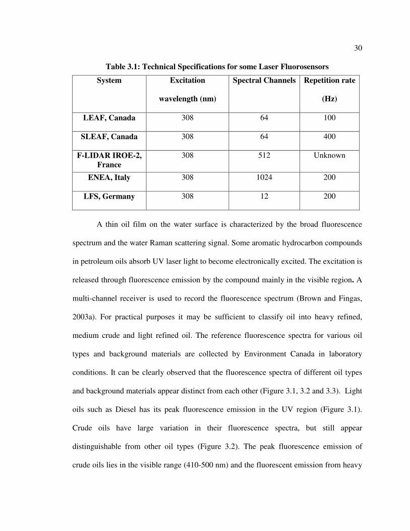
Table 3.1 describes the technical specifications for various laser fluorosensors (Adapted
from Brown and Fingas, 2003a).
30
Table 3.1: Technical Specifications for some Laser Fluorosensors
System Excitation
wavelength (nm)
Spectral Channels Repetition rate
(Hz)
LEAF, Canada 308 64 100
SLEAF, Canada 308 64 400
F-LIDAR IROE-2, France
308 512 Unknown
ENEA, Italy 308 1024 200
LFS, Germany 308 12 200
A thin oil film on the water surface is characterized by the broad fluorescence
spectrum and the water Raman scattering signal. Some aromatic hydrocarbon compounds
in petroleum oils absorb UV laser light to become electronically excited. The excitation is
released through fluorescence emission by the compound mainly in the visible region. A
multi-channel receiver is used to record the fluorescence spectrum (Brown and Fingas,
2003a). For practical purposes it may be sufficient to classify oil into heavy refined,
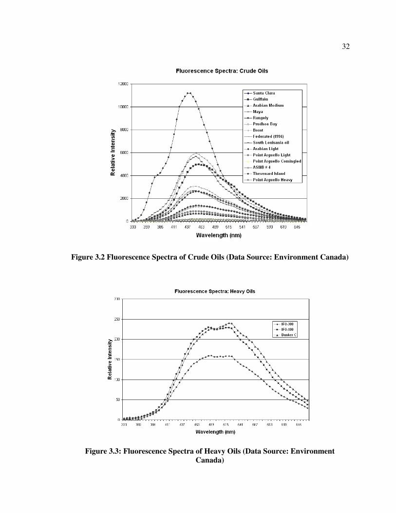
medium crude and light refined oil. The reference fluorescence spectra for various oil
types and background materials are collected by Environment Canada in laboratory
conditions. It can be clearly observed that the fluorescence spectra of different oil types
and background materials appear distinct from each other (Figure 3.1, 3.2 and 3.3). Light
oils such as Diesel has its peak fluorescence emission in the UV region (Figure 3.1).
Crude oils have large variation in their fluorescence spectra, but still appear
distinguishable from other oil types (Figure 3.2). The peak fluorescence emission of
crude oils lies in the visible range (410-500 nm) and the fluorescent emission from heavy

31
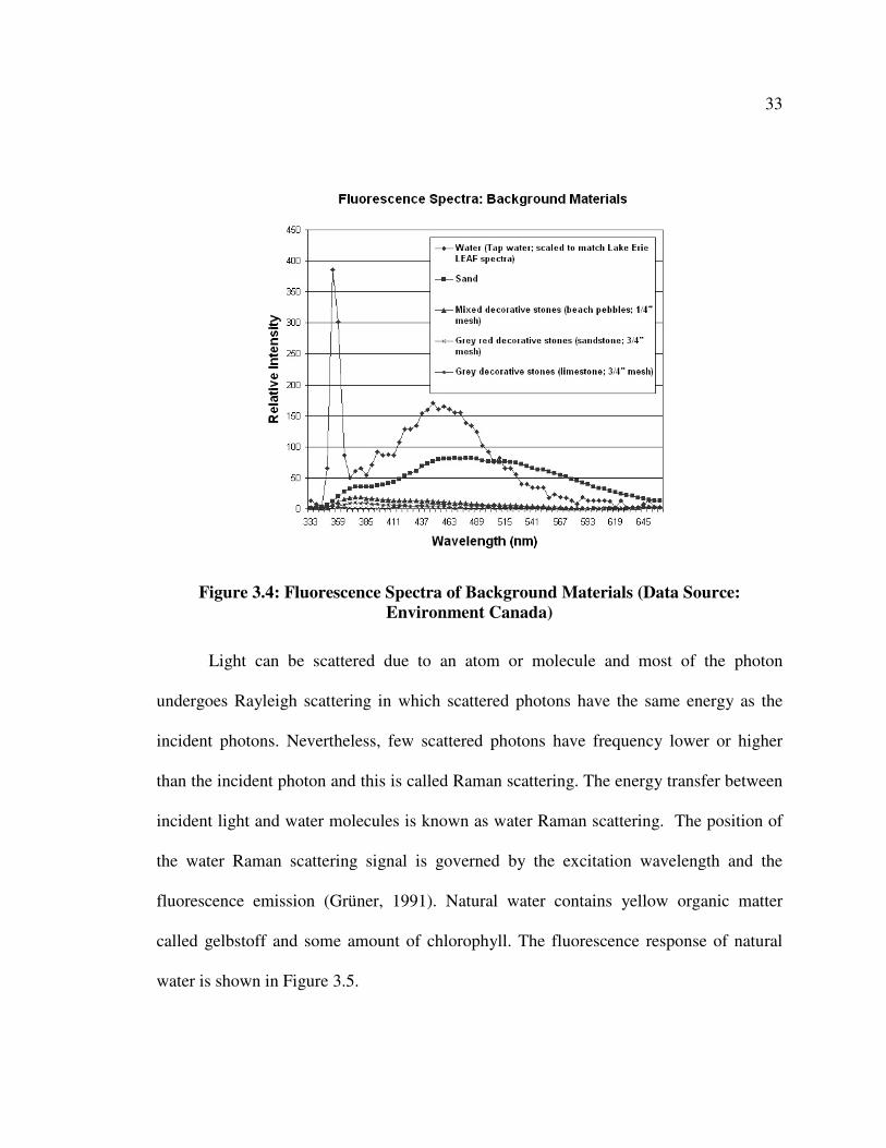
refined oils is considerably lower than others (Figure 3.3). Oil spills in coastal areas are
damaging and difficult to detect. An oil spill in an open sea tends to reach the coastal
regions due to various factors including wind and current. Possible background materials
include water, sand and stone. Figure 3.4 shows the fluorescence spectra of background
materials.
Figure 3.1: Fluorescence Spectra of Light Oils. Data Source: Environment Canada
32
Figure 3.2 Fluorescence Spectra of Crude Oils (Data Source: Environment Canada)
Figure 3.3: Fluorescence Spectra of Heavy Oils (Data Source: Environment Canada)
33
Figure 3.4: Fluorescence Spectra of Background Materials (Data Source: Environment Canada)
Light can be scattered due to an atom or molecule and most of the photon
undergoes Rayleigh scattering in which scattered photons have the same energy as the
incident photons. Nevertheless, few scattered photons have frequency lower or higher
than the incident photon and this is called Raman scattering. The energy transfer between
incident light and water molecules is known as water Raman scattering. The position of
the water Raman scattering signal is governed by the excitation wavelength and the
fluorescence emission (Grüner, 1991). Natural water contains yellow organic matter
called gelbstoff and some amount of chlorophyll. The fluorescence response of natural
water is shown in Figure 3.5.

34
Figure 3.5: Fluorescence Spectra of Natural Water for Excitation Wavelength as 308 nm (Adapted from Grüner, 1991)
The oil film on the water suppresses the water Raman scattering signal
corresponding to the absorption coefficient of the oil (Hoge and Swift, 1980). If the
excitation wavelength is 308 nm (XeCl laser) then the water Raman scattering signal is
observed at 344 nm. The water Raman scattering signal is useful for fluorescence
calibration as well as for estimating oil thickness to some extent (Brown and Fingas,
2003a). To obtain the oil thickness from the Raman signal depression data, the following
data must be known (Figure 3.6):
(1) Seawater background fluorescence from organic materials
(2) Oil fluorescence
The ratio of the Raman intensity measured above the oil slick and the Raman
intensity measured outside the oil slick is a function of thickness d of the oil film and the

35
attenuation coefficient of the oil film. The attenuation coefficient of a material is its
ability to reduce intensity of energy beam passing through it. The attenuation coefficient
of the oil depends upon the oil type. The relation can be represented in Equation 3.1
(Hoge and Swift, 1980).
Figure 3.6: Laser Induced Fluorescence (LIF) spectrum for Oil Slick and Sea Water
(Adapted from Hoge and Swift, 1980)
*1/( ) ln( / )d k k R Re r
= − + (3.1)
where d is the thickness of oil spill, R* is the Raman Intensity measured above the oil
slick, R is the Raman Intensity measured outside the oil slick in background water, e
k is
the attenuation coefficient of oil at the excitation wavelength, r
k is the attenuation
coefficient of oil at the Raman wavelength. Raman intensity is also used for correcting

36
the fluorescence signal for optical penetration depth in the water column. A fluorescence
signal normalized by Raman intensity indicates the concentration of fluorescent
substances. Laser fluorosensors cannot measure oil thickness greater than 10-20 microns
as UV laser light is completely absorbed by oil and cannot reach the underlying water
(Brown and Fingas, 2003b).
Various characteristics can be used for oil identification such as spectral shape,
the fluorescence decay time, the position of the fluorescent peak, the fluorescence yield,
the depression of water Raman scattering signal, and the variation of these parameters
with the excitation wavelength (Quinn et al., 1994). Fluorescence yield is the total
fluorescence emission for a given substance. The time at which the intensity becomes 1/e
of the original value is known as Fluorescence decay time. Fluorescence decay time can
be useful for the identification of oil in laboratory conditions, but its practical application
may be limited by a variety of factors in the field (Camagni, 1991). When oil undergoes
weathering due to environmental factors, its fluorescence properties also change.
However, the spectral shape changes are not significant and oils can still be distinguished
as light refined, crude and heavy refined oils (Jha et al., 2008b). The life time of the oil
can be significantly affected by natural weathering and consequently the fluorescence
decay time may not be able to classify weathered oil. The peak of the fluorescence return
for crude oils is centered between 420-490 nm while the peak of the fluorescence return
from chlorophyll is centered on 680 nm and hence the fluorescence emission from
chlorophyll can be easily distinguished from that from oil (Patsayeva et al., 2000). The
peak of fluorescence return from gelbstoff or yellow matter is centered on 420 nm and,
hence it may be difficult to detect crude oils on water rich with gelbstoff. Gelbstoff can
37
be present in high amounts in coastal areas. However, the fluorescence return from oil is
much larger in magnitude than water with high amount of CDOM and this can be useful
in differentiating oil from the water (Dick and Fingas, 1992). Hence, if the fluorescence
emission peak exceeds a threshold set for water then it can be used as the first indicator
for the presence of oil. The fluorescence emission peak depends on the target distance,
type of the oil, oil thickness and the amount of oil dispersed in water (Patsayeva et al.,
2000).
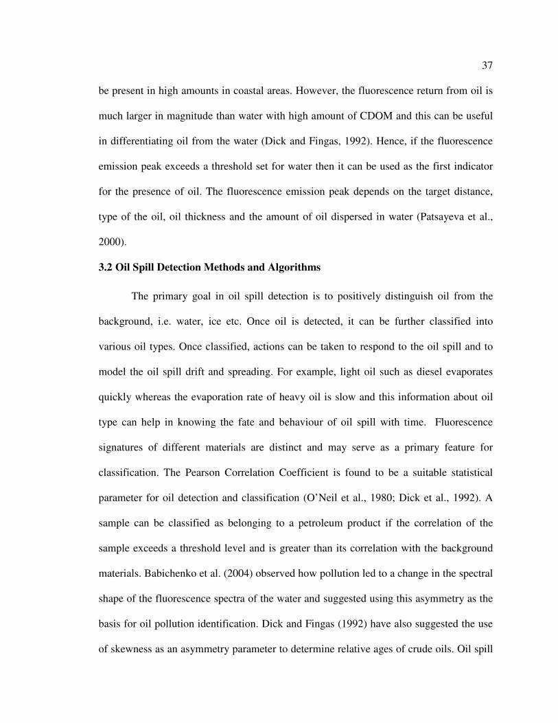
3.2 Oil Spill Detection Methods and Algorithms
The primary goal in oil spill detection is to positively distinguish oil from the
background, i.e. water, ice etc. Once oil is detected, it can be further classified into
various oil types. Once classified, actions can be taken to respond to the oil spill and to
model the oil spill drift and spreading. For example, light oil such as diesel evaporates
quickly whereas the evaporation rate of heavy oil is slow and this information about oil
type can help in knowing the fate and behaviour of oil spill with time. Fluorescence
signatures of different materials are distinct and may serve as a primary feature for
classification. The Pearson Correlation Coefficient is found to be a suitable statistical
parameter for oil detection and classification (O’Neil et al., 1980; Dick et al., 1992). A
sample can be classified as belonging to a petroleum product if the correlation of the
sample exceeds a threshold level and is greater than its correlation with the background
materials. Babichenko et al. (2004) observed how pollution led to a change in the spectral
shape of the fluorescence spectra of the water and suggested using this asymmetry as the
basis for oil pollution identification. Dick and Fingas (1992) have also suggested the use
of skewness as an asymmetry parameter to determine relative ages of crude oils. Oil spill

38
detection and classification can also be carried out based on the ratio of values of the
relative intensity of various spectral bands in the fluoresence spectra (Alaruri et al., 1995;
Quinn et al., 1994). Quinn et al. (1994) note that the emission spectra obtained using a
single excitation wavelength cannot be used to classify the oil into specific oil types but it
can classify the oil into three broad categories: light refined, medium crude and heavy
refined oil. Quinn et al. (1994) consider a number of parameters, including the spectral
and temporal characteristics of the fluorescence spectra of the material and use Principal
Component Analysis (PCA) to reduce the feature space (to a few significant PCs). PCA
has been widely used for oil classification (James and Dick, 1996; Alaruri et al., 1995).
For example, James and Dick (1996) discuss the advantages of using PCA over the
Pearson Correlation Coefficient. They note that PCA involves less computation and can
help in separating the mixed pixels, although it is assumed that materials are optically
thick which can be valid for littoral oil spills but may not be applicable for open ocean
spills. Moreover, they did not address the classification problems for dealing with in-situ
data which may require more than simply adding Gaussian noise. The Pearson
Correlation Coefficient and PCA have been widely used for oil spill detection and
classification, and the theory is described below. The Pearson Correlation Coefficient
( ρ ) yields the quantitative value of the correspondence between observed and reference
spectra (Equation 3.2).
2 22 2
N X Y X Yi i i i
i i i
N X X N Y Yi i i i
i i i i
ρ
−∑ ∑ ∑
= − −∑ ∑ ∑ ∑
(3.2)

39
where i
X and i
Y are the intensity values for the ith spectral band in reference and
observed spectra respectively and N is the number of spectral bands used in finding the
correlation. A correlation value of +1 indicates perfect correlation; a value of 0 indicates
no correlation; and a correlation value of -1 indicates perfect anti-correlation between the
reference and observed spectra (O’Neil et al., 1980).
The PC transformation is a linear transformation which produces uncorrelated and
noise segregated components. The data is transformed such that first few PCs have the
most variances. Accordingly, later components can be ignored. The Principal Component
Transformation (Y) may be expressed as in Equation 3.3.
TY A X= (3.3)
where A is the matrix of eigenvectors which diagonalizes the covariance matrix x
Σ of
original data (X) as expressed by Equations 3.4 and 3.5.
T
y xA AΣ = Σ (3.4)
1
2
0 0 0 0
0 0 0 0
. 0 . . .
. . . . 0
0 0 0 0
y
N
λ
λ
λ
Σ =
(3.5)
where 1λ , 2λ ,… Nλ are the eigenvalues of the matrix xΣ and 1λ > 2λ >… Nλ . The choice of
the matrix to find eigenvectors depends upon the application as second moment matrix
and correlation matrix can also be used instead of covariance matrix xΣ . Comprehensive
details about PCA can be found in Jackson (1991).
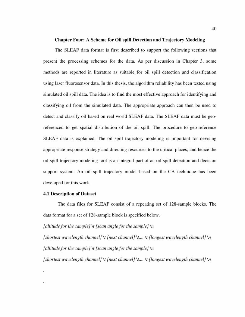
40
Chapter Four: A Scheme for Oil spill Detection and Trajectory Modeling
The SLEAF data format is first described to support the following sections that
present the processing schemes for the data. As per discussion in Chapter 3, some
methods are reported in literature as suitable for oil spill detection and classification
using laser fluorosensor data. In this thesis, the algorithm reliability has been tested using
simulated oil spill data. The idea is to find the most effective approach for identifying and
classifying oil from the simulated data. The appropriate approach can then be used to
detect and classify oil based on real world SLEAF data. The SLEAF data must be geo-
referenced to get spatial distribution of the oil spill. The procedure to geo-reference
SLEAF data is explained. The oil spill trajectory modeling is important for devising
appropriate response strategy and directing resources to the critical places, and hence the
oil spill trajectory modeling tool is an integral part of an oil spill detection and decision
support system. An oil spill trajectory model based on the CA technique has been
developed for this work.
4.1 Description of Dataset
The data files for SLEAF consist of a repeating set of 128-sample blocks. The
data format for a set of 128-sample block is specified below.
[altitude for the sample] \t [scan angle for the sample] \n
[shortest wavelength channel] \t [next channel] \t.... \t [longest wavelength channel] \n
[altitude for the sample] \t [scan angle for the sample] \n
[shortest wavelength channel] \t [next channel] \t.... \t [longest wavelength channel] \n
.
.
41
[altitude for the sample] \t [scan angle for the sample] \n
[shortest wavelength channel] \t [next channel] \t...... \t [longest wavelength channel] \n
[time of first sample] \t [latitude] \t [longitude] \t [heading] \t [pitch] \t [roll] \t [course
over ground] \t [ground speed] \n
The scan angle is given in degrees and the scanning pattern is elliptic with major
axis along the flight direction (7.6 x 5.3 degrees). The sampling rate is 350 Hz. The
minimum wavelength specified is 332.6 nm and the maximum wavelength is 662.8 nm.
The last line for the block which contains time, latitude and longitude applies to the
preceding 128-sample block. This sequence repeats until the End of File. “Time of first
sample” applies to the first sample of the 128-sample block and remaining time
references have been interpolated for the other samples.
4.2 Comparative Evaluation of Existing Methods for Oil Spill Detection
The reference laser fluorescence spectra for various petroleum products and
background materials provided by Environment Canada are used. The summary statistics
for various kinds of oils and background materials provide more insight into data
characteristics (Table 4.1, 4.2, 4.3, 4.4). The summary statistics is generated using
Microsoft excel for the reference laser fluorescence spectra data provided by
Environment Canada. Sum denotes the summation of intensity values over all the bands
and range denotes the difference between maximum and minimum intensity values for a
given material. Skewness is the measure of symmetry of dataset. It is zero for normal
distributions. If distribution has an asymmetric tail stretching towards more positive
values then skweness is positive otherwise skewness is negative. Skewness is positive for
light oils, crude oils and all background materials except sand whereas it is negative for
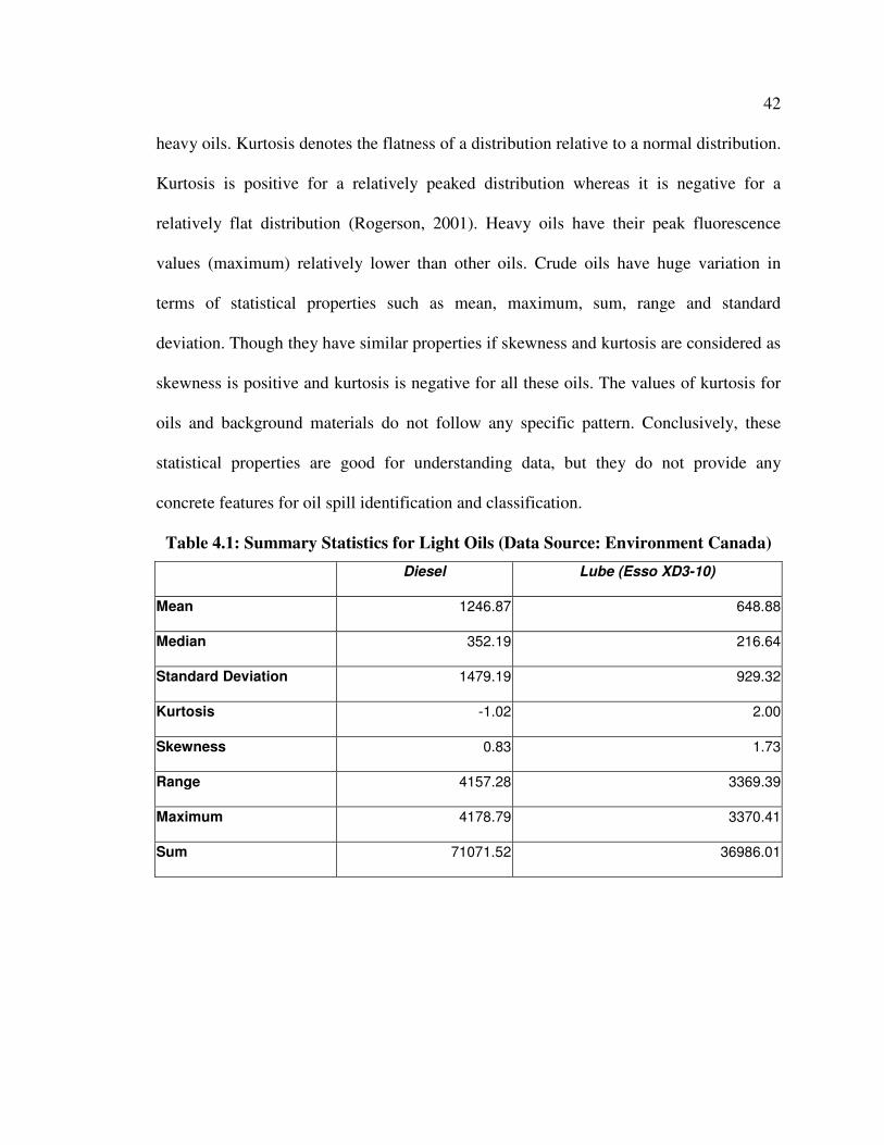
42
heavy oils. Kurtosis denotes the flatness of a distribution relative to a normal distribution.
Kurtosis is positive for a relatively peaked distribution whereas it is negative for a
relatively flat distribution (Rogerson, 2001). Heavy oils have their peak fluorescence
values (maximum) relatively lower than other oils. Crude oils have huge variation in
terms of statistical properties such as mean, maximum, sum, range and standard
deviation. Though they have similar properties if skewness and kurtosis are considered as
skewness is positive and kurtosis is negative for all these oils. The values of kurtosis for
oils and background materials do not follow any specific pattern. Conclusively, these
statistical properties are good for understanding data, but they do not provide any
concrete features for oil spill identification and classification.
Table 4.1: Summary Statistics for Light Oils (Data Source: Environment Canada)
Diesel Lube (Esso XD3-10)
Mean 1246.87 648.88
Median 352.19 216.64
Standard Deviation 1479.19 929.32
Kurtosis -1.02 2.00
Skewness 0.83 1.73
Range 4157.28 3369.39
Maximum 4178.79 3370.41
Sum 71071.52 36986.01

43
Table 4.2: Summary Statistics for Heavy Oils (Data Source: Environment Canada)
IFO-300 IFO-180 Bunker C
Mean 93.86 132.61 137.65
Median 95.88 136.28 144.30
Standard Deviation 50.22 74.55 75.79
Kurtosis -1.45 -1.46 -1.34
Skewness -0.13 -0.12 -0.23
Range 149.11 220.03 233.61
Maximum 159.71 229.59 239.97
Sum 5349.82 7558.56 7845.77
Table 4.3: Summary Statistics for Some Crude Oils (Data Source: Environment Canada)
Santa Clara Gullfaks Arabian Medium Maya Rangely
Mean 94.29 2202.82 335.88 105.74 1124.96
Median 88.63 1836.72 298.07 97.70 876.01
Standard Dev 54.52 1637.62 219.04 66.84 840.99
Kurtosis -1.44 -1.33 -1.35 -1.43 -1.25
Skewness 0.18 0.40 0.30 0.20 0.45
Range 160.11 4753.68 650.42 195.75 2504.43
Maximum 177.83 4961.90 701.16 210.60 2612.02
Sum 5374.37 125560.71 19145.28 6027.06 64122.49

44
Table 4.4: Summary Statistics for Background Materials (Data Source: Environment Canada)
Water Sand Beach Pebbles Sandstone Limestone
Mean 66.33 52.35 7.18 3.08 2.75
Median 55.40 53.21 6.06 2.45 1.63
Standard Deviation 55.42 22.20 5.61 2.21 2.65
Kurtosis -1.13 -1.31 -1.06 -0.80 0.95
Skewness 0.51 -0.17 0.50 0.63 1.38
Range 168.97 68.97 18.68 7.22 9.75
Maximum 170.95 81.76 18.75 7.34 9.75
Sum 3780.56 2983.98 409.15 175.54 156.59
For each reference material, 20 simulated fluorescence spectra are generated by
adding 10% white Gaussian noise to the reference fluorescence spectra. Some sample
fluorescence spectra generated from the reference spectra of light oil are shown in Figure
4.1. As there are 25 reference materials, the total number of simulated fluorescence
spectra is 500.

45
Figure 4.1: Sample Simulated Data Generated for Light Oil by adding 10% Gaussian Noise
The Raman scattering bands are not considered for the classification since this
feature commonly occurs in fluorescence spectra over the water surface. The most
general approach to classify and detect oil involves the determination of the spectral
distance between the simulated and the reference spectra. The observed spectra can be
labelled as that reference material for which this spectral distance is minimum. In the
second approach, PCA is applied to the collection of the reference spectra and only those
PCs which contribute significantly to the variance in the reference data are considered for
creating the PC space. The oil classification is based on the spectral distance between the
observed fluorescence spectra and the reference spectra in the PC space. The third
approach is based on Pearson Correlation Coefficient for classifying and detecting oil. In
the fourth approach, the ratios of the relative intensities in different spectral bands (for

46
each pair) are used as a distinguishing feature. When considering 58 spectral bands, the
number of ratio combinations will be 1653 ( 58
2C ), the idea therefore is to regard the
distinguishing combinations as relevant. For this purpose, the variance-to-mean ratio
(VMR) is calculated to find variability for each ratio combination for all the reference
materials. The six ratio combinations with the highest VMR ratio were considered and
then PCA was applied to find the only significant components. The spectral distance
between observed and reference spectra was used as the basis for the classification in this
newly formed PC space. A scheme has been developed for the classification of the
observed SLEAF data based on the results of algorithms applied to simulated data.
The PCs for all the reference spectra were computed. The plot of eigenvalues
depicting variance contained in their corresponding PCs is shown in Figure 4.2. Only the
first three PCs contribute significantly to the data’s variance and hence the classification
is based on only these PCs. The PC loading plot explains the contribution of the original
bands in forming the PCs. As mentioned earlier, the minimum wavelength for data
acquisition is 332.6 nm and the maximum wavelength is 662.8 nm. There are 64 receiver
channels to capture the fluorescence spectrum. This implies that the band 1 corresponds
to the wavelength of 332.6 nm whereas the band 64 corresponds to the wavelength of
662.8 nm. The approximate difference between two consecutive bands is 5.2 nm. For the
first PC, it can be observed that the contribution of bands increases with the band increase
till the band 24 and then the contribution starts decreasing (Figure 4.3). The second and
third PCs have more uniform contribution from all original bands than the first PC. The
scatter plot for all reference materials in the PC space is shown in Figure 4.4. The light
oils are shown in blue; the heavy oils are shown in green; the crude oils are shown in red,

47
the water is shown in cyan; the sand is shown in black and stone is shown in magenta.
The used legend remains the same for Figure 4.5 and 4.7. The light oils and the crude oils
are well separated from background materials, but the heavy oils seem closer to the
background materials in the PC space. The identification of the heavy oil on the
background materials can be problematic. The 2D scatter plot is then created to check the
separability more closely in the PC space created by PC1 and PC2 (Figure 4.5). The
reference materials are found to be well separated in the 2D space as well.
The six ratio components having the highest VMR were identified and PCA was
applied to find the significant components. The plot of eigenvalues for the covariance
matrix is determined for these six ratio components (Figure 4.6). It can be observed that
only the first PC is significant. The 3D scatter plot for reference materials in PC space for
the ratio components is shown in Figure 4.7. The reference materials are closely placed n
this PC space except the heavy oils. Thus, the oil spill identification and classification
results using this PC space can give incorrect results. Moreover, the technique based on
the ratio components can be sensitive to noise in data. This can work well if the effect of
noise is uniform over the whole fluorescence spectrum as in that case the ratios will not
be affected. Ratio Components can be useful in case of real SLEAF data as this technique
only considers the ratios of relative intensities in different bands and not the actual values
of the relative intensities of the target materials. The classification results based on the
simulated data using PCs for ratio components were not satisfactory. Accordingly, it was
concluded that the ratio components are not a reliable feature for oil spill detection and
classification. As previously mentioned, the classification process should successfully
classify the oil into the following three broad categories: light refined, crude and heavy
48
refined oil. Hence, the results are categorized into specific and aggregate (broad)
categories. The successful specific classification implies that a particular oil remains
classified in the same category after adding 10% white Gaussian noise. The results of
classification using the other algorithms with the simulated data are shown in Table 4.5.
The background materials are successfully classified with 100% accuracy by all three
approaches. All algorithms are highly successful in classifying oil into the three broad
categories of light refined, crude and heavy refined oil with classification accuracy
around 100%. This implies that all these three approaches can detect and classify oils into
the broad categories even if the data is noisy. The classification accuracy for all three
approaches in specific categories for light oils is 100%. The reference sample set of the
light oils only consists of two oils namely “Diesel” and “Lube (Esso XD3-10) and
specific classification into these two oils are possible by all three approaches. The
classification accuracy for specific classification in case of the heavy oils is around 95%
when General and PCA approach is used. On the other hand, classification accuracy is
only 83% when Pearson Correlation Coefficient is used. Hence, General and PCA
approach can be more reliable than Pearson Correlation Coefficient for classification into
specific categories in case of the heavy oils. The classification accuracy for the
classification into specific categories for the crude oils is around 90% when using
General and PCA approach. The performance of Pearson Correlation Coefficient is the
worst for specific oil classification among all the methods used. The results are
particularly bad in case of classifying the crude oils into specific categories as the
accuracy is only 42%. The low specific oil classification accuracy in case of crude oils
when using Pearson Correlation Coefficient can be due to high correlation among the oils
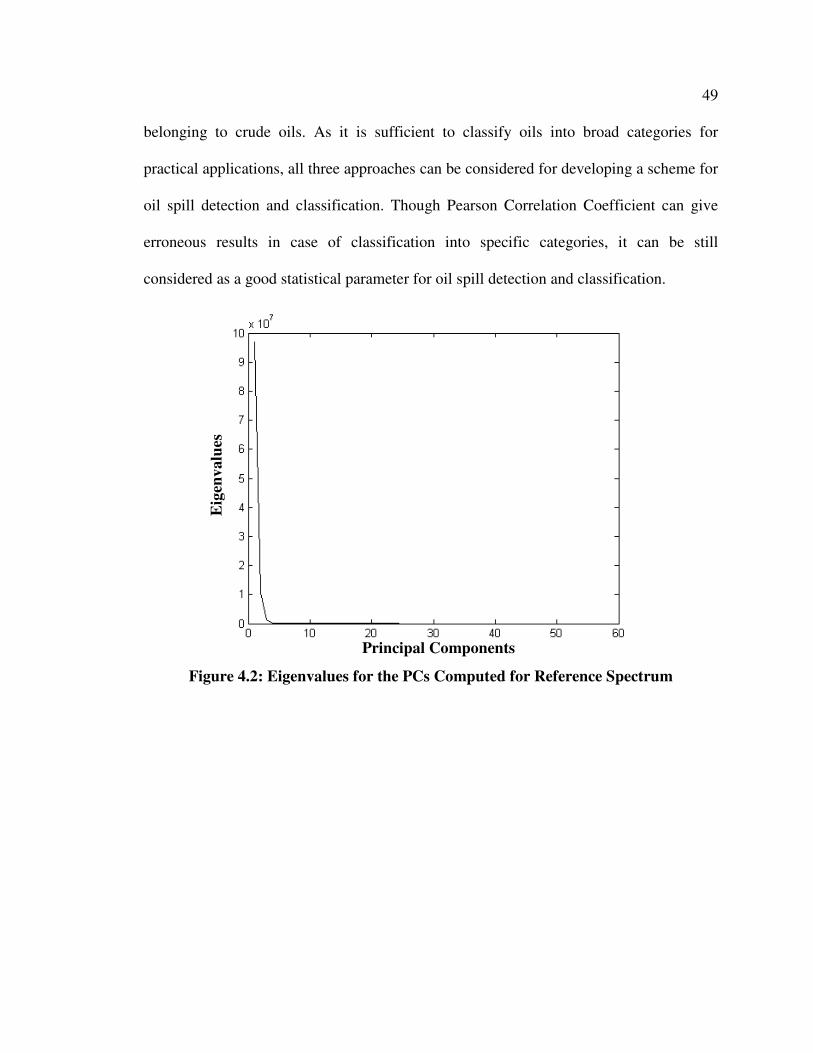
49
belonging to crude oils. As it is sufficient to classify oils into broad categories for
practical applications, all three approaches can be considered for developing a scheme for
oil spill detection and classification. Though Pearson Correlation Coefficient can give
erroneous results in case of classification into specific categories, it can be still
considered as a good statistical parameter for oil spill detection and classification.
Figure 4.2: Eigenvalues for the PCs Computed for Reference Spectrum
Eig
env
alu
es
Principal Components
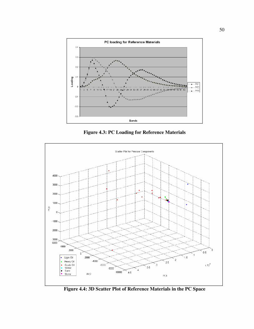
50
Figure 4.3: PC Loading for Reference Materials
Figure 4.4: 3D Scatter Plot of Reference Materials in the PC Space

51
Figure 4.5: 2D Scatter Plot of Reference Materials in the PC Space (PC1 and PC2)
Figure 4.6: Eigenvalues for the PCs Computed for Ratio Components
Eig
env
alu
es
Principal Components

52
Figure 4.7: 3D Scatter Plot of Reference Materials in the PC Space for Ratio
Components

53
Table 4.5: Classification Results using Various Algorithms for Simulated Data
Type General (%) PCA (%) Correlation (%)
Light Oil Broad 100 100 100
Specific 100 100 100
Crude Oil Broad 100 100 99.7
Specific 90.7 90 42
Heavy Oil Broad 100 100 100
Specific 95.8 95 83.3
Water 100 100 100
Sand 100 100 100
Stone 100 100 100
4.3 A Proposed Oil Spill Detection and Classification Scheme
Oil’s fluorescence emission depends on various factors such as the oil thickness,
the distance from the target and atmospheric conditions. If PCA or General approach is
used, the observed SELAF data has to be normalized so that it can be compared to the
reference spectra collected in the laboratory (Almhdi, 2007). The data normalization is a
difficult process as the information about the oil thickness, the distance from the target
and atmospheric conditions are needed. It is difficult to model effect of these conditions
on the fluorescence spectra. Moreover, these information are often not available in the
field conditions. Classification of data using Pearson Correlation Correlation depends
only on the shape of the fluorescence spectra and not the total fluorescence emission.
Pearson Correlation Correlation is used to classify the data in the case of the actual

54
SLEAF data due to the erroneous nature of data normalization. Classification based on
the correlation coefficient will not yield reliable results if high correlations between
reference materials exist. Accordingly, it is imperative to investigate the correlation
between various reference materials. The correlation map for different materials is shown
in Figure 4.8. This correlation map is generated using MATLAB. Features 1-2 belong to
light oil, features 3-5 belong to heavy oil, features 6-20 belong to crude oils, feature 21 is
water and features 22-25 are other background materials. The oil spill detection and
classification scheme is shown in Figure 4.9. High correlation between petroleum
products and background materials is the primary challenge for accurate oil spill
detection. If maximum correlation between reference and observed spectra is greater than
threshold ‘th0’ then classification can be reliable otherwise the observed point can be
labelled as ‘unknown’. Light oils have a high correlation with the stones, but the
fluorescence emission from stones are significantly lower than that from light oils and
this can be a distinguishing factor (see Figure 3.1 and Figure 3.4). A threshold ‘th1’ can
be selected. Heavy oils (IFO 180 and IFO 300) and some crude oils (e.g. Arabian
Medium) have a high correlation with sand, but the fluorescence emission from sand is
significantly lower than those for these oils (Figure 3.3 and Figure 3.4). A threshold (th2)
of fluorescence emission may be used to distinguish sand from oils. If fluorescence
emission of the observed material is greater than this threshold (th2) it may belong to
heavy oils or some crude oils. As peak of fluorescence emission from crude oils are
significantly higher than heavy oils a threshold ‘th 3’ can be chosen. Some crude oils
such as Thevenard Island, ASMB#4 and South Louisiana Oil have a high correlation with
the water. Marine oil spills can cause serious environmental degradation, and hence it is

55
important that a reliable mechanism is established to distinguish oil from the water.
Compared to the fluorescence emissions of water, those from the correlated crude oils are
high (Figure 3.2), and thus a threshold ‘th4’ can be set for the minimum peak
fluorescence emission. If the peak fluorescence emission is less than this threshold, we
consider it to be water. Oceanic water may contain gelbstoff and the amount of gelbstoff
can be considerably high in coastal regions. The fluorescence emission from gelbstoff
may also be high. The Raman suppression can be a useful parameter to assist in
distinguishing the fluorescence spectra from oil and gelbstoff. Oil suppresses the water
Raman scattering signal considerably in comparison to the gelbstoff and, therefore the
ratio of the peak fluorescence emission and the water Raman scattering signal for oil will
be much higher than that of water containing gelbstoff. An appropriate threshold ‘th4’
can be selected such that the material will be assumed to be oil if the ratio is higher than
the threshold and as water otherwise. Selection of the values of the six thresholds
indicated in the scheme i.e. th0, th1, th2, th3 , th4 and th5 should be done with great care
as this can affect the oil spill detection and classification results. The ground truth is
required to get the appropriate values of these thresholds. The developed oil spill
detection and classification scheme can be used for finding oil from the area where
ground truth is available. The thresholds can be adjusted to get the correct results. This
process can be repeated for other areas where ground truth is available to get the suitable
values of these thresholds. The ground truth could not be obtained for this research and
hence initial values of these thresholds are obtained by carefully analysing reference
fluorescence spectra. These values are later adjusted based on the results obtained by
applying developed oil spill detection and classification scheme on real world SLEAF

56
data and feedback from ESTD, Canada. The set of thresholds which are used for the oil
spill detection and classification scheme in this research is shown in Table 4.6.
Table 4.6: Typical Values of Thresholds for Oil Spill Detection and Classification Scheme
Thresholds th0 Th1 th2 th3 th4 th5
0.9 200 130 250 500 3
Figure 4.8: Correlation Map for Reference Fluorescence Spectra

57
Figure 4.9: Scheme for Oil Spill Detection and Classification
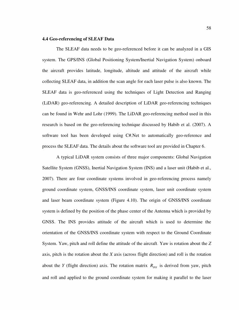
58
4.4 Geo-referencing of SLEAF Data
The SLEAF data needs to be geo-referenced before it can be analyzed in a GIS
system. The GPS/INS (Global Positioning System/Inertial Navigation System) onboard
the aircraft provides latitude, longitude, altitude and attitude of the aircraft while
collecting SLEAF data, in addition the scan angle for each laser pulse is also known. The
SLEAF data is geo-referenced using the techniques of Light Detection and Ranging
(LiDAR) geo-referencing. A detailed description of LiDAR geo-referencing techniques
can be found in Wehr and Lohr (1999). The LiDAR geo-referencing method used in this
research is based on the geo-referencing technique discussed by Habib et al. (2007). A
software tool has been developed using C#.Net to automatically geo-reference and
process the SLEAF data. The details about the software tool are provided in Chapter 6.
A typical LiDAR system consists of three major components: Global Navigation
Satellite System (GNSS), Inertial Navigation System (INS) and a laser unit (Habib et al.,
2007). There are four coordinate systems involved in geo-referencing process namely
ground coordinate system, GNSS/INS coordinate system, laser unit coordinate system
and laser beam coordinate system (Figure 4.10). The origin of GNSS/INS coordinate
system is defined by the position of the phase center of the Antenna which is provided by
GNSS. The INS provides attitude of the aircraft which is used to determine the
orientation of the GNSS/INS coordinate system with respect to the Ground Coordinate
System. Yaw, pitch and roll define the attitude of the aircraft. Yaw is rotation about the Z
axis, pitch is the rotation about the X axis (across flight direction) and roll is the rotation
about the Y (flight direction) axis. The rotation matrix INS
R is derived from yaw, pitch
and roll and applied to the ground coordinate system for making it parallel to the laser

59
unit coordinate system. The procedure of deriving the rotation matrix can be found in
detail in Habib (2009).
The laser unit has a laser scanner which measures distance to the ground points
and scans angles. The origin of the laser unit coordinate system is at the laser firing point.
The Y direction for the laser unit coordinate system is assumed to be in the flight
direction and the X axis is considered across the flight direction. The Z direction is
assumed to be in the vertical direction and perpendicular to the XY plane. The laser beam
coordinate system share same origin as the laser unit coordinate system. The scan angles
define the rotational offset between the laser unit coordinate system and the laser beam.
There is spatial and rotational offset/boresighting between the GNSS/INS unit and the
laser unit. The spatial offset between the GNSS/INS system and the laser unit can be
denoted by a vector GPr
with respect to the GNSS/INS coordinate system. The rotational
offset is the orientation of the laser unit with respect to the GNSS/INS system. The
rotation matrix R∆ is applied to the GNSS/INS coordinate system for making it parallel
to the laser unit coordinate system. scanR is the rotation matrix derived using scan angles
and it is applied to laser unit coordinate system to make it parallel to the laser beam
coordinate system. The range vector ρv
denotes the coordinates of target point in laser
beam coordinate system.
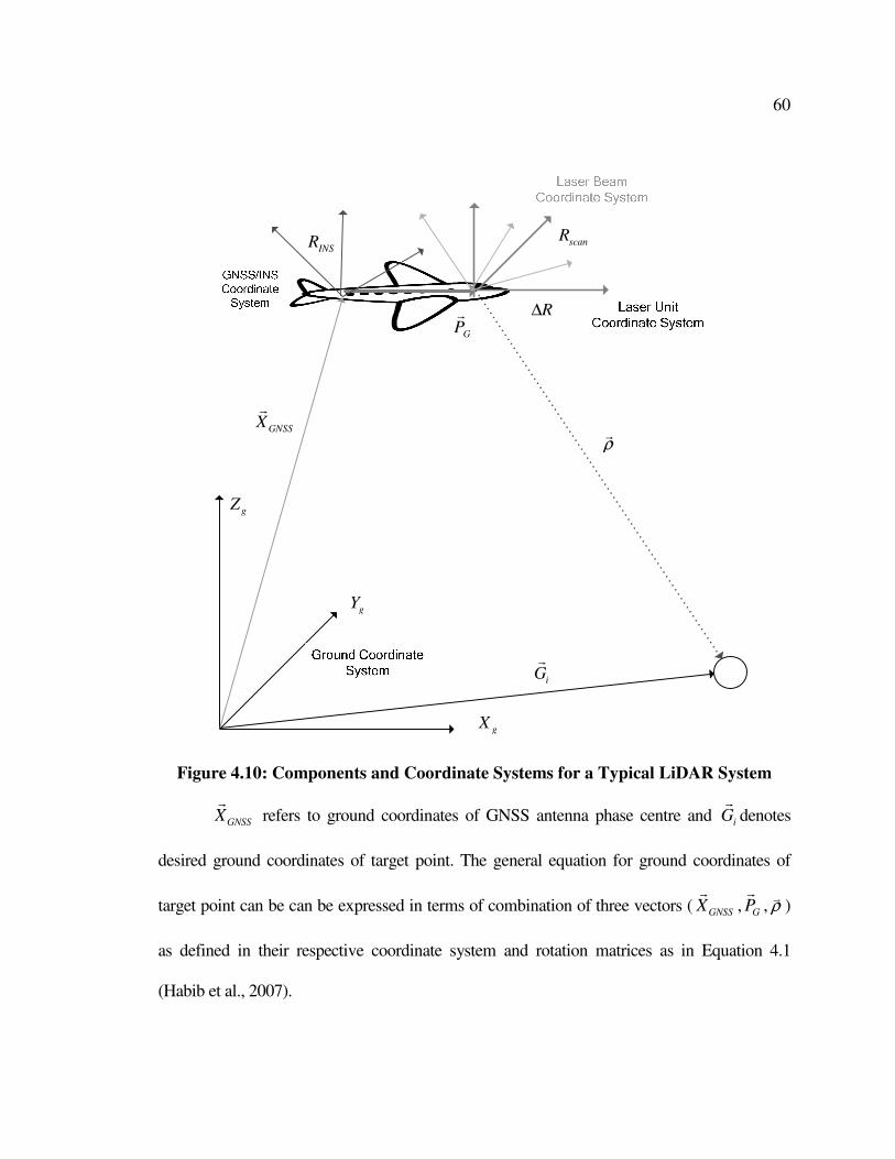
60
ρr
iGr
INSR
gX
gY
gZ
GPr
scanR
R∆
GNSSXr
Figure 4.10: Components and Coordinate Systems for a Typical LiDAR System
GNSSXr
refers to ground coordinates of GNSS antenna phase centre and iGr
denotes
desired ground coordinates of target point. The general equation for ground coordinates of
target point can be can be expressed in terms of combination of three vectors ( GNSSXr
, GPr
, ρv
)
as defined in their respective coordinate system and rotation matrices as in Equation 4.1
(Habib et al., 2007).

61
0
0
i
i
i
i GNSS INS G INS scan
X
G Y X R P R RR
Z ρ
= = + + ∆ −
r r r (4.1)
The general Equation 4.1 can not be used for geo-referencing SLEAF data due to
the limitation in the acquired SLEAF dataset. There is no range ( ρ ) information
provided for SLEAF dataset. No information is provided in the dataset about spatial and
rotational boresighting/offset. Considering that spatial accuracy is not so critical in this
application, the effect of spatial and rotational boresighting/offset will be ignored. Thus,
the GNSS/INS coordinate system will be identical to the laser unit coordinate system
with respect to the ground coordinate system. (Figure 4.11).
/GNSS INSXr
iGr
INSR
gX
gY
gZ
INSX
INSY
INSZ
Figure 4.11: Coordinate Systems for SLEAF
62
As explained in section 4.1 for SLEAF dataset description, the dataset consists of
repeating sets of 128-sample block. The position provided by the GNSS system
GNSSXr
belongs to the first sample for that sample block, but the aircraft moves forward
and a term speedPr
is added to GNSSXr
to compensate for the movement because of the speed
of the aircraft. The position of the target in the laser unit coordinate system can be
measured using scan angle tθ at time ‘t’ and total field of views Tα and βT (Figure 4.12
and Figure 4.13). As SLEAF is used for detecting oil in ocean, we can assume that the
surface for a given set of sample block has no significant variation in elevation from the
reference. speedPr
and laserPr
are defined in the GNSS/INS coordinate system or laser unit
coordinate system as in Equation 4.2 and Equation 4.3.
0
*
0
speedP speed time
=
r (4.2)
laser
X
P Y
H
= −
r (4.3)
where X, Y, -H are the coordinates of target point observed in laser unit coordinate
system. The position of the object in the ground coordinates system iGr
is a combination
of three vectors 0t
GNSSXr
, speedPr
and laserPr
defined in the coordinate systems specified above
(Equation 4.4).
63
0 0
0
0
* * *
0
i
i
i
t tt t t t
i GNSS INS speed INS laser GNSS INS INS
X X
G Y X R P R P X R V t R Y
HZ
t t t
= = + + = + ∆ + −
= + ∆
r r r r r
(4.4)
where,
iGr
: Ground coordinates of the object point under consideration
0t
GNSSXr
: Ground coordinates of the GNSS antenna phase center at time 0t
speedPr
: Aircraft movement in GNSS/INS coordinate system in time t∆
laserPr
: The position of the target object in laser unit coordinate system.
0t
GNSSXr
is originally given in terms of latitude and longitude which must be transformed
into a suitable projected coordinate system to facilitate further calculation. A projected
coordinate system is based on a geographic coordinate system and locations are specified
by x, and y coordinates in a grid (ArcGIS Desktop Help, 2009). Any projection system
would introduce certain distortion. The conical projection system is suitable for mid-
latitude region. The Lambert conformal conic projection is commonly used conical
projection system for USA and Canada and has been used in this research. The latitude
and longitude derived from the onboard GPS are projected into Lambert conformal conic
projection and hence GNSSXr
denotes the transformed coordinates. t
INSR can be derived by
using the values of yaw, pitch and roll provided in the dataset. Altitude H is also provided
in the dataset. The only problem is to derive expression for X and Y in terms of altitude of
the aircraft, two total angular field of views ( Tα and βT) and scan angle tθ at time t

64
(Figure 4.12). SLEAF uses an elliptical scanner to capture the data. A nutating mirror is
part of the elliptical scanning system which is used to form elliptical footprints on the
ground. Tα is the total angular field of view with respect to the flight direction, and βT is
the total angular field of view with respect to the across flight direction (Figure 4.12). As
specified in the data description section of this chapter, values of Tα and Tβ are 7.6 and
5.3 degrees respectively.
Tβ
Tα
Figure 4.12: Angular Field of Views for Elliptical Scanner
The major axis is along the flight direction as specified in SLEAF data description. The
equation of ellipse can be expressed by Equation 4.5.
2 2
2 21
x y
a b+ = (4.5)
where, ‘a’ is the semi-minor axis and ‘b’ is the semi-major axis of the ellipse. The
relationship between the angular field of views Tα , Tβ and a, b can be evaluated using
principles of trigonometry as expressed by Equation 4.6 if altitude of aircraft is assumed
as 1.

65
tan( / 2)
tan( / 2)
T
T
a
b
β
α
=
= (4.6)
Putting values of a and b in Equation 4.5, we get Equation 4.7 (Habib et al., 2007).
2 2
2 21
tan ( / 2) tan ( / 2)T T
x y
β α+ = (4.7)
A typical laser foot print at time ‘t’ can be represented as in Figure 4.13. tx and ty are the
position of target point with respect to the laser unit coordinate system. tx and ty can be
expressed in term of scan angle tθ and tr as follows
cos
sin
t t t
t t t
x r
y r
θ
θ
=
= (4.8)
Now, ( tx , ty ) point lies on the ellipse and will satisfy Equation 4.5. Equation 4.9 can be
obtained by substituting x and y with tx and ty in Equation 4.7.
tθ
( )tt yx,tr
X
Y
Figure 4.13: Angular Position of a Point in Elliptical Footprint
2 2 2 2
2 2
cos sin1
tan ( / 2) tan ( / 2)
t t t t
T T
r rθ θ
β α+ = (4.9)

66
After solving Equation 4.9, the radius tr can be given as in Equation 4.10 (Habib et al.,
2007).
)2/(tansin)2/(tancos
)2/tan()2/tan(
2222
TtTt
TT
trβθαθ
αβ
+= (4.10)
The values of ( tx , ty ) can be obtained from Equation 4.8. Now if the altitude of aircraft
is H, X and Y for Equation 4.3 can be obtained as follows (Equation 4.11 and Equation
4.12).
*tX x H= (4.11)
HyY t *= (4.12)
The ground coordinates of target points can now be estimated using Equation 4.4.
As described earlier, the SLEAF data set is composed of sets of 128-samples.
Each sample consists of two lines. The first line of each sample contains altitude, scan
angle; these values are stored in an Array say ‘dataArray’. The second line contains
fluorescence spectra for that sample. The scheme developed for oil spill detection and
identification is used for assigning material type to that sample. This information is stored
as feature type ‘dataArray’. This ‘dataArray’ is added to an arraylist say ‘data’. This
process is repeated till we reach 128th
sample or 256th
line in the SLEAF text file. Now,
we have scan angle, altitude and feature type stored for each sample as ‘dataArray’ in the
arraylist ‘data’. At the 257th
line for the set of 128-samples, the latitude, longitude,
attitude and speed are provided corresponding to the first sample. Based on the geo-
referencing process discussed here, the ground coordinates of each 128-samples is

67
obtained and stored. The whole process is repeated for all set of 128-samples in the
SLEAF data file until we reach the end of file.
4.5 Oil Spill Trajectory Modeling using Cellular Automata
CA is made up of identical n-dimensional cells. The value of the physical quantity
under consideration at a cell denotes the local state of that cell. The interactions between
cells are assumed to be local and the neighbourhood of a cell is defined by adjacent and
diagonal cells. The state at a particular cell is calculated from states of neighbouring cells
and the state of that cell in previous time step based on a CA local rule, which is typically
the same for all cells in the CA. A two dimensional CA can have four bordering cells
(von Neumann neighbourhood) or eight bordering cells (Moore neighbourhood) as shown
in Figure 4.14 and 4.15 respectively.
*
Figure 4.14: The Von Neumann Neighborhood
*
Figure 4.15: The Moore Neighborhood
If Moore neighbourhood is considered, the cell state 1
,
t
i jC+
at time t+1 can be defined as
function of eight neighbourhood cells as in Equation 4.13.
1
, 1, 1 1, 1, 1 , 1 , , 1 1, 1 1, 1, 1( , , , , , , , , )t t t t t t t t t t
i j i j i j i j i j i j i j i j i j i jC F C C C C C C C C C+
− − − − + − + + − + + += (4.13)
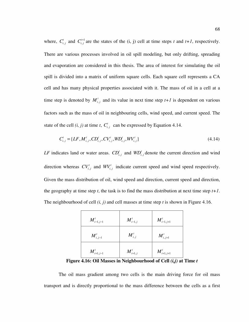
68
where, ,
t
i jC and 1
,
t
i jC+
are the states of the (i, j) cell at time steps t and t+1, respectively.
There are various processes involved in oil spill modeling, but only drifting, spreading
and evaporation are considered in this thesis. The area of interest for simulating the oil
spill is divided into a matrix of uniform square cells. Each square cell represents a CA
cell and has many physical properties associated with it. The mass of oil in a cell at a
time step is denoted by ,
t
i jM and its value in next time step t+1 is dependent on various
factors such as the mass of oil in neighbouring cells, wind speed, and current speed. The
state of the cell (i, j) at time t, ,
t
i jC can be expressed by Equation 4.14.
, , , , , ,{ , , , , , }t t t t t t
i j i j i j i j i j i jC LF M CD CV WD WV= (4.14)
LF indicates land or water areas. ,
t
i jCD and ,
t
i jWD denote the current direction and wind
direction whereas ,
t
i jCV and ,
t
i jWV indicate current speed and wind speed respectively.
Given the mass distribution of oil, wind speed and direction, current speed and direction,
the geography at time step t, the task is to find the mass distribution at next time step t+1.
The neighbourhood of cell (i, j) and cell masses at time step t is shown in Figure 4.16.
1, 1
t
i jM − −
1,
t
i jM −
1, 1
t
i jM − +
, 1
t
i jM − ,
t
i jM , 1
t
i jM +
1, 1
t
i jM + −
1,
t
i jM +
1, 1
t
i jM + +
Figure 4.16: Oil Masses in Neighbourhood of Cell (i,j) at Time t
The oil mass gradient among two cells is the main driving force for oil mass
transport and is directly proportional to the mass difference between the cells as a first

69
order approximation. For example, the oil mass at cell (i, j) due to oil mass in cell (i-1, j)
can be given as in Equation 4.15.
1
, , 1, ,( )t t t t
i j i j i j i jM M m M M+
−= + − (4.15)
where, m is a constant and governs the portion of the mass difference transferred to the
neighbouring cell. The mass transport between diagonal cell will be less than the mass
transport between adjacent cells and it can be modeled by introducing an additional
diagonal factor ‘d’. Therefore, considering all eight neighbouring cells 1
,
t
i jM+
can be given
by Equation 4.16 (Karafyllidis, 1997).
1
, , 1, , , 1 , , 1 ,
1, , 1, 1 , 1, 1 ,
1, 1 , 1, 1 ,
( ) ( ) ( )
( ) ( ) ( )
( ) ( )
t t t t t t t t
i j i j i j i j i j i j i j i j
t t t t t t
i j i j i j i j i j i j
t t t t
i j i j i j i j
M M m M M m M M m M M
m M M md M M md M M
md M M md M M
+
− − +
+ − − − +
+ − + +
= + − + − + −
+ − + − + − +
− + −
(4.16)
No oil transport between cells is possible if a neighbouring cell represents a land. The
‘LF’ flag for a cell indicates whether a cell represents land or not. An additional term to
take care of evaporation can be added (Equation 4.17), where tT is the temperature of
environment, m
t is the model time step and p is a constant (Karafyllidis, 1997).
1
, , 1, , , 1 , , 1 ,
1, , 1, 1 , 1, 1 ,
1, 1 , 1, 1 ,
( ) ( ) ( )
( ) ( ) ( )
( ) ( )
t t t t t t t t
i j i j i j i j i j i j i j i j
t t t t t t
i j i j i j i j i j i j
t t t t t
i j i j i j i j m
M M m M M m M M m M M
m M M md M M md M M
md M M md M M pt T
+
− − +
+ − − − +
+ − + +
= + − + − + −
+ − + − + − +
− + − −
(4.17)
Direction coefficients are defined to take wind and current effects into
consideration. For example, direction coefficient for south direction can be represented as
in Equation 4.18 (Karafyllidis, 1997).

70
,, ,
,
, max
,
, max
t
i j t tw ci j i j
t
i j
tci j
t
i j
twi j
S S S
CVS
CV
WVS R
WV
= +
=
=
(4.18)
,t
wi j
S is called wind direction constant and ,
tci j
S is called current direction constant. ,
t
i jWV
and ,
t
i jCV are wind and current speeds in the cell (i, j) at time step t. R is wind-current
transformation factor and used to transform wind speed to wind-driven current speed.
Typical values of R lie between 0.03 to 0.16. max
WV and max
CV are the maximum wind
and current speed in that area. The final equation considering all the factors can be
written as expressed by Equation 4.19 (Karafyllidis, 1997).
1
, , , 1, , , , 1 ,
, , 1 , , 1, , , 1, 1 ,
, 1, 1 , , 1, 1
((1 ) ) ((1 ) )
((1 ) ) ((1 ) ) ((1 ) )
((1 ) ) ((1 )
t t t t t t t t
i j i j i j i j i j i j i j i j
t t t t t t t t t
i j i j i j i j i j i j i j i j i j
t t t t t
i j i j i j i j i j
M M m N M M m W M M
m E M M m S M M md NW M M
md NE M M md SW M
+
− −
+ + − −
− + + −
= + + − + + − +
+ − + + − + + −
+ + − + + ,
, 1, 1 ,
)
((1 ) )
t
i j
t t t t
i j i j i j m
M
md SE M M pt T+ +
− +
+ − −
(4.19)
The value of m and d for the time step of 30 minutes was found to be 0.0014 and 0.18
respectively (Karafyllidis, 1997).

71
Chapter Five: Results and Discussion
The methodology for oil spill detection and classification was discussed in
Chapter 4. Many existing algorithms used for oil spill detection and classification may
work well for simulated data with additive noise, but they have been found to be
ineffective for real world data, which can be attributed to a number of reasons. The
fluorescence emission captured in the actual data acquisition process may get affected by
various factors including the distance of the sensor from the target and oil thickness.
SLEAF data from 2004 and 2006 Environment Canada flights are used for testing
methods for oil spill detection. The data collected in 2004 was acquired on the east coast
of Canada and the data collected in 2006 is from the area around Vancouver Island.
Figure 5.1 shows the location of the study area. These data were collected by
Environment Canada to check for illegal oil discharges in the ocean. As laser
fluorosensors can detect even the sheen of oil from the background materials, SLEAF
data is expected to detect even small traces of any small oil discharge. Data collection
and the methods have been elaborated in Brown et al. (2004a) and Brown et al. (2006b).
The identification of oil in coastal areas can be challenging due to various factors such as
the presence of large amounts of suspended materials and the lower depth of the water
column.
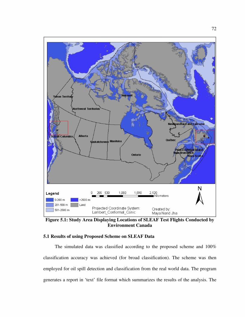
72
Figure 5.1: Study Area Displaying Locations of SLEAF Test Flights Conducted by Environment Canada
5.1 Results of using Proposed Scheme on SLEAF Data
The simulated data was classified according to the proposed scheme and 100%
classification accuracy was achieved (for broad classification). The scheme was then
employed for oil spill detection and classification from the real world data. The program
generates a report in ‘text’ file format which summarizes the results of the analysis. The

73
sample from the ‘text’ file is provided below. The results are saved in a personal
geodatabase which also facilitates further GIS analysis.
X: -2104601.22966204, Y: 2043406.30789842 Max Correlation is: 0.983976865895914 This spectra belongs to Material 0 Diesel
X: -2104601.41274777, Y: 2043406.28800501 Max Correlation is: 0.974989134340548 This spectra belongs to Material 0 Diesel
X: -2104601.59583349, Y: 2043406.2681116 Max Correlation is: 0.971220277558307 This spectra belongs to Material 0 Diesel
X: -2104601.77891921, Y: 2043406.24821819 Max Correlation is: 0.956692802038031 This spectra belongs to Material 20 Water
X: -2104601.96200493, Y: 2043406.22832478 Max Correlation is: 0.971905956257307 This spectra belongs to Material 20 Water
X: -2104602.14509066, Y: 2043406.20843137 Max Correlation is: 0.957579084095699 This spectra belongs to Material 20 Water
X: -2104602.32817638, Y: 2043406.18853796 Max Correlation is: 0.951878238195994 This spectra belongs to Material 20 Water
Light oil slick (diesel) is detected in the area around Vancouver Island which is
consistent with Environment Canada observations. Observed fluorescence spectra
containing thick and thin oil films are shown in Figure 5.2 and Figure 5.3, respectively.
The spectra showing water rich with gelbstoff and turbid water are shown in Figure 5.4
and Figure 5.5, respectively. The oil was not found in the SLEAF Canadian east coast
data. East coast regions contain high doses of gelbstoff as evident from the high
fluorescence emissions of water in that area (Figure 5.6).

74
Figure 5.2: Observed Fluorescence Spectra for Thick Oil Film of Diesel in Vancouver Island
Figure 5.3: Observed Fluorescence Spectra for Thin Film of
Diesel in Vancouver Island Area

75
Figure 5.4: Fluorescence Spectra of Water (Gelbstoff) in Vancouver Island Area
Figure 5.5: Fluorescence Spectra of Turbid Water in Vancouver Island Area

76
Figure 5.6: Fluorescence Spectra of Water (Gelbstoff) in East Coast of Canada
5.2 Oil Spill Disaster Products
Oil spill disaster products in map format can be a useful tool for oil spill
responders and decision makers. Maps can present enormous information in a
conceptually simple way. Maps are an essential component of planning and management
of an oil spill. The system can integrate the spill locations and trajectory vectors with
additional data from the database to provide utilities such as the oil spill location map, oil
spill trajectory map, oil spill risk map, oil spill affected area map and oil spill emergency
response maps. These maps can be used in managing the equipment and resources such
as booms, skimmers and chemicals for oil spill clean up and containment operations. A
base GIS map is first created based on common features required for all oil spill disaster
products. Base GIS map includes bathymetry layer, layer containing street network, layer

77
having provinces, layer containing major cities etc. Oil spill information can be combined
with base map to create oil spill location map. Oil spill trajectory map is created using
prediction of trajectory of oil spill along with the base map. The Oil Spill Risk Map
explains the risk associated with an oil spill. The estimated trajectory of oil spill can be
combined with infrastructure and environmental data to evaluate the risk with respect to a
particular oil spill. Oil Spill Affected Area Map can be derived by using the actual extent
and spread of an oil spill. The actual damage caused by an oil spill can be estimated using
this map. Oil Spill Emergency Response Map provides the locations important to the
emergency response for the oil spill. For example, GIS layers indicating police stations,
emergency response centers, government agencies oil spill access points, road networks,
etc can be combined to formulate an effective response mechanism.
The geo-referenced SLEAF data from the Canadian east coast is shown in Figure
5.7. Many SLEAF flight lines can be seen around this area, but no oil discharge is
detected. Diesel discharge is detected around Vancouver Island area as shown in Figure
5.8. Elliptical footprints of SLEAF can be seen in this Figure. Diesel points are separated
from these elliptical foot prints and are combined with appropriate GIS layers to get oil
spill location map (Figure 5.9). Oil spill location map gives general information about an
oil spill and its surroundings. Oil Spill Emergency Response Map serves as important
tool for oil spill responder as it can help in taking quick and informed decisions (Figure
5.10). Any information which can be useful for oil spill emergency response agencies
such as police stations, emergency response centers, can be a part of this map. The exact
information about locations of police stations, hospitals, disaster support centers, oil spill
response agencies are not freely available and, hence some arbitrary locations are

78
assumed for the sake of this work. Oil spill trajectory is generated based on an imaginary
oil spill incident specified in oil spill trajectory modeling tool. Oil spill trajectory is
modeled based on assumed wind and current magnitude and direction. Oil spill trajectory
map is created combining predicted oil spill trajectory with base map (Figure 5.11).
Environmental information presented in map form can be useful for estimating damages
due to an oil spill as well as directing resources to proper locations. ESI map is a crucial
part of the system and can greatly assist disaster managers in taking decisions. ESI maps
for Canada is not freely available and, hence for illustration purposes ESI map for
Southern California, USA is shown in Figure 5.12. This ESI map is based on the data
provided by NOAA. The ESI map has coastal shorelines graded from 1 to 10, where 1
indicates the least environmental sensitivity and 10 indicates the highest environmental
sensitivity. ESI map also has other information useful for oil spill response planning such
as locations of biological resources and human-use resources.

79
Figure 5.7: Georeferenced and Processed SLEAF Data in East Coast of Canada
Figure 5.8: Oil Spill Detected around Vancouver Island

80
Figure 5.9: Oil Slick Extracted from SLEAF Data around Vancouver Island
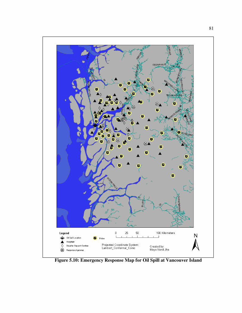
81
Figure 5.10: Emergency Response Map for Oil Spill at Vancouver Island

82
Figure 5.11: Oil Spill Trajectory Map with Assumed Parameters for Trajectory Modeling

83
Figure 5.12: ESI map for the Shoreline of Southern California (Source: NOAA)
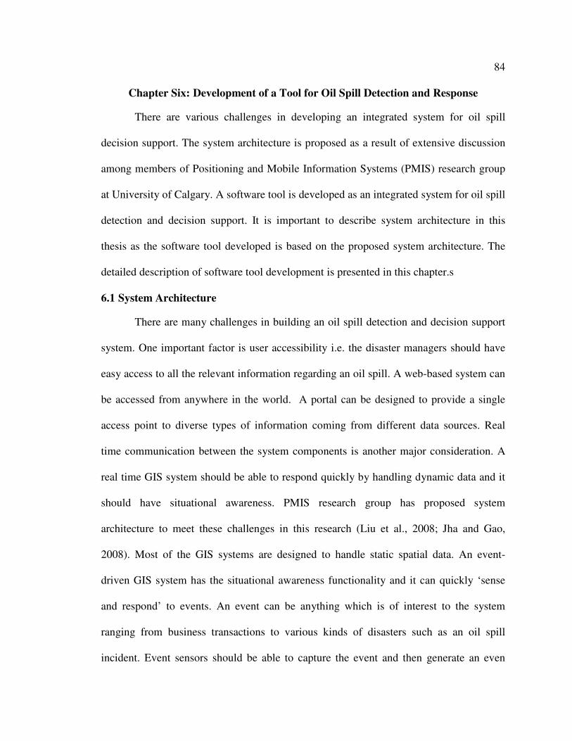
84
Chapter Six: Development of a Tool for Oil Spill Detection and Response
There are various challenges in developing an integrated system for oil spill
decision support. The system architecture is proposed as a result of extensive discussion
among members of Positioning and Mobile Information Systems (PMIS) research group
at University of Calgary. A software tool is developed as an integrated system for oil spill
detection and decision support. It is important to describe system architecture in this
thesis as the software tool developed is based on the proposed system architecture. The
detailed description of software tool development is presented in this chapter.s
6.1 System Architecture
There are many challenges in building an oil spill detection and decision support
system. One important factor is user accessibility i.e. the disaster managers should have
easy access to all the relevant information regarding an oil spill. A web-based system can
be accessed from anywhere in the world. A portal can be designed to provide a single
access point to diverse types of information coming from different data sources. Real
time communication between the system components is another major consideration. A
real time GIS system should be able to respond quickly by handling dynamic data and it
should have situational awareness. PMIS research group has proposed system
architecture to meet these challenges in this research (Liu et al., 2008; Jha and Gao,
2008). Most of the GIS systems are designed to handle static spatial data. An event-
driven GIS system has the situational awareness functionality and it can quickly ‘sense
and respond’ to events. An event can be anything which is of interest to the system
ranging from business transactions to various kinds of disasters such as an oil spill
incident. Event sensors should be able to capture the event and then generate an even

85
object which can be further processed in the system (Liu et al., 2008). Event driven GIS
system can be understood as similar to nervous system in our body. The basic
components of an event-driven GIS system are events, services, orchestration (event
processes) and the Enterprise Service Bus (ESB). ESB is a crucial part of an event-driven
GIS system as it facilitates a robust environment for accessing events and processes. Any
system can attach to ESB with built-in “publish and subscribe” facilities without
interfering with other existing systems attached to ESB. Another advantage of ESB is that
applications developed in multiple programming languages can interact with each other
via ESB. Various system components are described below.
• Sensors that generate events: These may include call centers, satellites or airborne
images, CCTV etc for oil spill accidents.
• Internet portal: It provides a centralized service for oil spill detection and decision
support.
• Web-GIS services: These services can generate oil spill disaster products
including oil spill location and trajectory maps, risk map and emergency response
maps. Location based services (LBS) can be also part of Web-GIS services.
• Orchestrations (Event Processes): These event processes include business logic
for oil spill disaster response such as oil spill image analysis, laser fluorosensor
data processing, trajectory analysis, risk analysis and emergency response
analysis.
• Other systems that are interested in receiving/exchanging advanced events
generated from Web-GIS or oil spill management system can be registered into
the system. Potential system components can be following:

86
o Fleet management system
o Other emergency systems
o Hospital management systems
o Government service system
o Applications in police department
o Other applications developed for oil spills by other departments
• Database Management System: All output results and relevant input data will be
stored in database. A robust database is needed to facilitate easy retrieval and
manipulation of information.
• Enterprise Service Bus: ESB provides the environment to access events and
services. TIBCO Enterprise Message Service by TIBCO software Inc is popular
software to facilitate real time flow of information and this will be used as ESB in
our system.
The use case diagram for the integrated system for oil spill response developed
for this research is shown in Figure 6.1. There can be two primary users for this system.
The first kind of users can be laser fluorosensor (SELAF) data providers. They can use
this system to check if SLEAF dataset captured for a particular area has any oil. The
other important user can be oil spill disaster manager. Oil spill disaster manager can also
have access to the SLEAF datasets and he/she can use the laser fluorosensor data
processing tool to analyse SLEAF data for oil. The oil spill reporting tool is available
which can be used to report an oil spill at a given location. GIS analysis tool can be used
for detailed spatial analysis and can be useful for directing appropriate resources to the oil
spill incident location. The system can be defined for more use cases if low-level design

87
is available. Different system components can be made available to different users based
on their responsibility and role. The system design as proposed by PMIS research group
is shown in Figure 6.2. The laser fluorosensor data source processing system, oil spill
reporting tool, oil spill trajectory modeling tool, GIS analysis tool and any other system
components can communicate with each other using ESB. Laser fluorosensor data
processing system is developed in this thesis utilizing the oil spill detection and
classification scheme developed in this research. The software tool developed in this
research can generate a personal geodatabase containing oil spill information when
SELAF data and the reference spectra files are provided. This personal geodatabase can
be then published to ESB. Oil spill reporting tool can be used to report an oil spill
incident and this event can be published to ESB. Any application interested in getting
information about a new oil spill can be subscribed to ESB. GIS components have been
developed to report an oil incident and model oil spill trajectory. The development of
software tool is explained in detail in the next section.
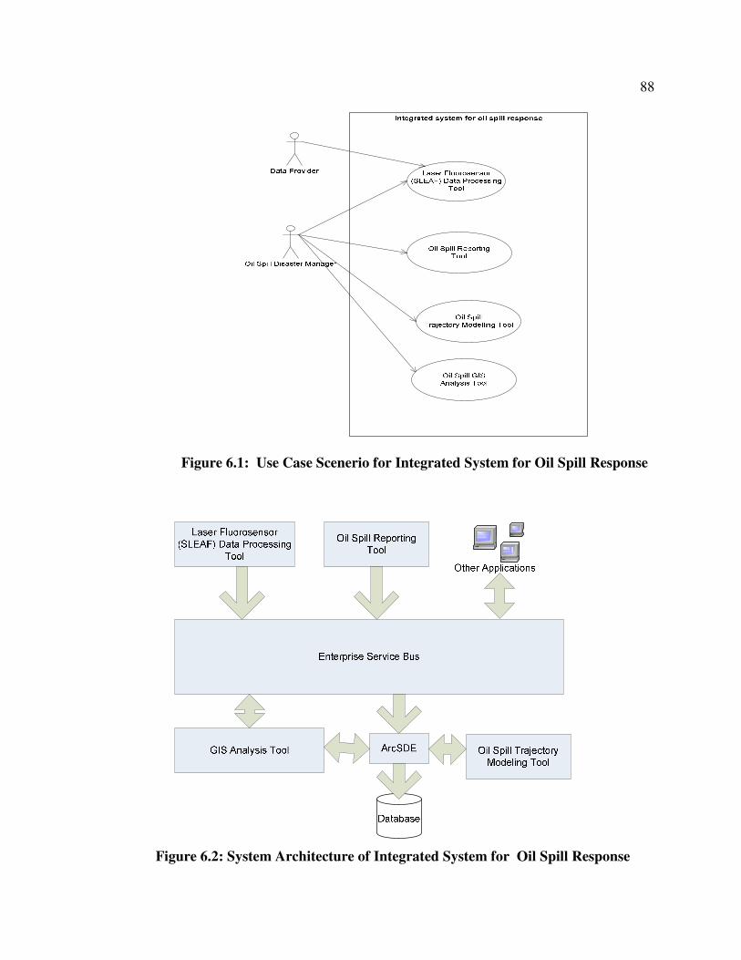
88
Figure 6.1: Use Case Scenerio for Integrated System for Oil Spill Response
Figure 6.2: System Architecture of Integrated System for Oil Spill Response
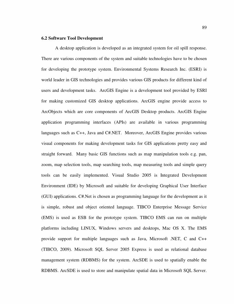
89
6.2 Software Tool Development
A desktop application is developed as an integrated system for oil spill response.
There are various components of the system and suitable technologies have to be chosen
for developing the prototype system. Environmental Systems Research Inc. (ESRI) is
world leader in GIS technologies and provides various GIS products for different kind of
users and development tasks. ArcGIS Engine is a development tool provided by ESRI
for making customized GIS desktop applications. ArcGIS engine provide access to
ArcObjects which are core components of ArcGIS Desktop products. ArcGIS Engine
application programming interfaces (APIs) are available in various programming
languages such as C++, Java and C#.NET. Moreover, ArcGIS Engine provides various
visual components for making development tasks for GIS applications pretty easy and
straight forward. Many basic GIS functions such as map manipulation tools e.g. pan,
zoom, map selection tools, map searching tools, map measuring tools and simple query
tools can be easily implemented. Visual Studio 2005 is Integrated Development
Environment (IDE) by Microsoft and suitable for developing Graphical User Interface
(GUI) applications. C#.Net is chosen as programming language for the development as it
is simple, robust and object oriented language. TIBCO Enterprise Message Service
(EMS) is used as ESB for the prototype system. TIBCO EMS can run on multiple
platforms including LINUX, Windows servers and desktops, Mac OS X. The EMS
provide support for multiple languages such as Java, Microsoft .NET, C and C++
(TIBCO, 2009). Microsoft SQL Server 2005 Express is used as relational database
management system (RDBMS) for the system. ArcSDE is used to spatially enable the
RDBMS. ArcSDE is used to store and manipulate spatial data in Microsoft SQL Server.

90
ArcSDE acts as a bridge between user and RDBMS and user has to deal with ArcSDE
without caring about particulars of RDBMS.
Figure 6.5 shows the part of the software displaying general information about the
system and the tools integrated in the system that are available to the user for oil spill
detection and decision support. The main input for SLEAF data processing is a text file
which contains information about observed fluorescence spectra for each target point.
The reference data is required which consists of fluorescence spectra of oils and
background materials collected in laboratory conditions. Laser fluorosensor data
processing software component can accept input SELAF file and the reference file from
the user. Thresholds can be specified by the user for the oil spill detection and
classification process or the default values may be used (Figure 6.6, 6.7). The laser
fluorosensor data processing tool processes data based on the proposed oil spill detection
and classification scheme. Every sample point is geo-referenced and then classified to
determine the oil traces. At the end of this process, a geodatabase containing locations of
each sample and associated feature type is obtained. This information should be
published to TIBCO EMS so that any applications interested in receiving this information
can get it via TIBCO EMS. TIBCO EMS accepts messages in form of XML only. The
geodatabase is converted into XML feature class and then published to TIBCO EMS. The
laser fluorosensor data processing process can be explained graphically by a flow chart
(Figure 6.3).

91
Figure 6.3: SLEAF Data Processing and Analysis Flow Chart
A detailed report is also generated which provides more information about the oil
spill detection and classification process. An oil spill incident can also be reported by
simply specifying location, date and amount and type of the oil spill (Figure 6.8).
Oil spill trajectory can be modeled by using the ‘Trajectory Modeling’ tool which
is based on the previously described CA model. Vector grids for oil mass distribution are
created using ‘Hawth’s Analysis Tool’ which is a freely available GIS tool for spatial
analysis (Figure 6.4). The detailed information about ‘Hawth’s Analysis Tool’ can be
found at Spatial Ecology Website (Spatial ecology, 2009). The grids for wind and current
information can also be added to the system to provide information about wind and
current velocity for each grid.
92
Figure 6.4: Hawth’s Analysis Tool for Creating Vector Grids
In the trajectory modeling tool, user is provided with default values of a number
of parameters, but it can be changed according to the user’s experience and knowledge
about the environmental settings (Figure 6.9, 6.10). Users click on grid where oil spill is
reported and input the required information and the ‘Save’ button stores this information
into the database (Figure 6.11). The spread of the spill is provided to the user once he/she
clicks on the ‘Model Trajectory’ button (Figure 6.12). GIS analysis tool is provided for
advanced GIS analysis (Figure 6.13). Many GIS functions such as map manipulation
tools, map searching tools, map measuring tools and simple query tools are made
available to the user by using ArcGIS Engine Map Control. Advanced users such as
Disaster Managers will have access to this tool. Oil spill disaster products are available

93
via this tool and other layers can be added by users if desired (Figure 6.14, 6.15, 6.16).
More components can be added to the system to enhance functionality of the system.
Figure 6.5: Software Tool Providing General Information about the Prototype System
Figure 6.6: Laser Fluorosensor Data Processing Part of the System

94
Figure 6.7: Dialog Box Showing that Processing of Laser Fluorosensor Data is Complete
Figure 6.8: Tool for Oil Spill Incident Reporting

95
Figure 6.9: Oil Spill Trajectory Modeling Tool Showing Options for Selecting Different Oil Types
Figure 6.10: Oil Spill Trajectory Modeling Tool Showing Options for Selecting Different Measurement Type for Oil

96
Figure 6.11: Saved Oil Spill Information in Oil Spill Trajectory Modeling Tool
Figure 6.12: Trajectory of Oil Spill after Time Interval of 150 Minutes
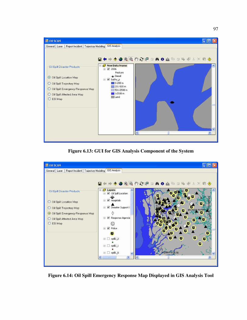
97
Figure 6.13: GUI for GIS Analysis Component of the System
Figure 6.14: Oil Spill Emergency Response Map Displayed in GIS Analysis Tool

98
Figure 6.15: Oil Spill Trajectory Map Displayed in GIS Analysis Tool
Figure 6.16: ESI Map Displayed in GIS Analysis Tool

99
Chapter Seven: Conclusions and Recommendations
Oil spills causes significant damage to economy and environment and proper oil
spill contingency planning can reduce response time and assist oil spill responders. The
research aimed to develop an oil spill detection system based on laser fluorosensor data.
Additional GIS tools were developed to assist oil spill responders in case of an oil spill.
7.1 Conclusions
Oil spill surveillance is an important part of oil spill contingency planning.
Current remote sensing sensors have been evaluated in terms of their usefulness for
detecting and monitoring oil spills. Laser fluorosensors were found to be the best
available sensor for oil spill surveillance as they can detect oil on various backgrounds
including ice and the shoreline. However, no single sensor had capability to provide all
the information needed for oil spill surveillance. Real time remote sensing data is
essential for oil spill response so that resources can be immediately directed to sensitive
areas for cleaning and containment operations.
The characteristics of laser fluorosensors were studied in detail in this research.
SLEAF operated by Environment Canada was found to successfully detect oil in test
flights by Environment Canada. An oil detection and classification scheme can make use
of various features such as spectral shape, the fluorescence decay time, the position of the
fluorescent peak, the fluorescence yield, the depression of water Raman scattering signal,
and the variation of these parameters with the excitation wavelength. The broad
fluorescence spectrum and water Raman scattering properties was found to be reliable in
order to improve oil spill detection and classification. Various algorithms were evaluated
in terms of their ability to detect and classify oil from simulated data as well as actual
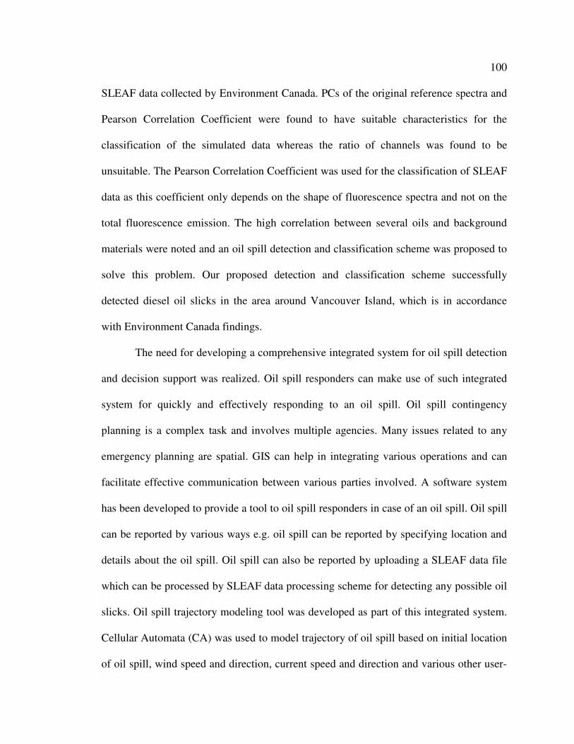
100
SLEAF data collected by Environment Canada. PCs of the original reference spectra and
Pearson Correlation Coefficient were found to have suitable characteristics for the
classification of the simulated data whereas the ratio of channels was found to be
unsuitable. The Pearson Correlation Coefficient was used for the classification of SLEAF
data as this coefficient only depends on the shape of fluorescence spectra and not on the
total fluorescence emission. The high correlation between several oils and background
materials were noted and an oil spill detection and classification scheme was proposed to
solve this problem. Our proposed detection and classification scheme successfully
detected diesel oil slicks in the area around Vancouver Island, which is in accordance
with Environment Canada findings.
The need for developing a comprehensive integrated system for oil spill detection
and decision support was realized. Oil spill responders can make use of such integrated
system for quickly and effectively responding to an oil spill. Oil spill contingency
planning is a complex task and involves multiple agencies. Many issues related to any
emergency planning are spatial. GIS can help in integrating various operations and can
facilitate effective communication between various parties involved. A software system
has been developed to provide a tool to oil spill responders in case of an oil spill. Oil spill
can be reported by various ways e.g. oil spill can be reported by specifying location and
details about the oil spill. Oil spill can also be reported by uploading a SLEAF data file
which can be processed by SLEAF data processing scheme for detecting any possible oil
slicks. Oil spill trajectory modeling tool was developed as part of this integrated system.
Cellular Automata (CA) was used to model trajectory of oil spill based on initial location
of oil spill, wind speed and direction, current speed and direction and various other user-

101
defined parameters. Various oil spill disaster products such as oil spill location map, oil
spill risk map and oil spill emergency response map can be made available to the disaster
managers.
The system architecture to meet the research objectives was discussed. ESB can
provide environment for communication between various system components such as
remote sensing image processing system, Web-GIS and database. More components can
be added to the system during the development as all components are loosely coupled or
independent of each other and only communicate via ESB. A prototype desktop
application was developed using Visual Studio 2005 (C#.NET) to demonstrate the
feasibility of such as system. ArcGIS Engine was used to develop spatial components of
the system. Microsoft SQL Server 2005 Express was used as RDBMS for the system.
ArcSDE was used to handle spatial data query and manipulation and it acts as bridge
between users and the RDBMS. The developed prototype system displays the feasibility
of creating a fully operational comprehensive integrated system for oil spill disaster
management. Though, system is specifically designed for handling oil spill disasters, but
can be easily extended to handle other disasters such as Urban Fire, Floods etc.
7.2 Recommendations
The objective of this research is to provide a reliable oil spill detection system
based on laser fluorosensor data. Some additional tools were developed to assist oil spill
responders in case of an oil spill. This research contributed in realizing this goal to some
extent, but still a lot of work is needed to achieve the full-fledged system. Reliable oil
spill detection and classification is an important part of this work as this can
tremendously help in reducing ambiguity in terms of identifying and responding to an oil

102
spill. Laser fluorosensor can be a useful input for a real-time system as it can be
processed for detecting and classifying oil in real-time. An oil spill detection and
classification scheme is developed for reliable oil spill detection and classification, but
further research is needed to improve and check the reliability of our outlined oil spill
detection and classification scheme.
The oil spill trajectory model used in this research is based on many
simplifications and has ignored some processes involved in deciding fate and behaviour
of oil spill. Oil spill trajectory modeling is complicated and extensive research is needed
to understand various aspects of the modeling.
The goal of the research is to develop a web-based GIS system so that it can be
accessible from anywhere in the world. A desktop system was developed in this research,
but more work is needed to convert this system to a web-based system. The system
architecture is designed for an oil spill detection and decision support system and clearly
defines system components at high-level. A detailed low-level design based on the user
requirements should be prepared based on the real requirements of oil spill disaster
managers in case of an oil spill.
103
References
Alaruri, S.D., M. Rasas, O. Alamedine, S. Jubian, F. Al-Bahrani and M. Quinn, “Remote
Characterization of Crude and Refined Oils using a Laser Fluorosensor System”,
Optical Engineering, 34:01, pp. 214-221, 1995.
Almhdi, K.H., P. Valigi, V. Gulbinas, R. Westphal and R. Reuter, “Classification with
Artificial Neural Networks and Support Vector Machines: Application to Oil
Fluorescence Spectra”, EARSeL eProceedings, 6, 2007.
ArcGIS Desktop Help, Topic: Projected Coordinate System.
http://webhelp.esri.com/arcgisdesktop/9.3/index.cfm?TopicName=About_projected_c
oordinate_systems. Last accessed on Aug 14, 2009.
Armstrong, M.P. and P.J. Densham, “Database organization startegies for spatial decision
support system”, International Journal of Geographical Information Systems, 4:1, pp.
3-20, 1990.
Babichenko, S., A. Dudelzak and L. Poryvkina, “Laser Remote Sensing of Coastal and
Terrestrial Pollution by FLS-LiDAR”, EARSeL eProceedings, 3, 2004.
Brebbia, C.A., Oil Spill Modeling and Processes, WIT Press, UK, 2001.
Brekke, C. and A. Solberg, “Oil spill detection by satellite remote sensing”, Remote
Sensing of Environment, 95, pp.1 –13, 2005.
Brown, C. and M. Fingas, “Review of Oil Spill Remote Sensing”, Spill Science &
Technology Bulletin, 4.4, pp.199-208, 1997.

104
Brown, C. and M. Fingas, “New space-borne sensors for oil spill response”, International
SPILL Conference, American Petroleum Institute, Washington, DC, pp. 911-916,
2001a.
Brown, C. and M. Fingas, “Upcoming Satellites: Potential Applicability to Oil Spill
Remote Sensing”. Proceedings of the 24th Arctic and Marine Oil Spill Program
(AMOP) Technology Seminar, Environment Canada, Ottawa, ON, Canada, pp. 495-
505, 2001b.
Brown, C. and M. Fingas, “Review of the Development of Laser Fluorosensors for Oil
Spill Application”, Marine Polution Bulletin, 47, pp. 477–484, 2003a.
Brown, C. and M. Fingas, “Development of airborne oil thickness measurements”,
Marine Pollution Bulletin, 47, pp. 485–492, 2003b.
Brown, C. and M. Fingas, “A review of current global oil spill surveillance, monitoring
and remote sensing capabilities”, Proceedings of the 28th Arctic and Marine Oil Spill
Program (AMOP) Technical Seminar, Environment Canada, Ottawa, ON, Canada,
pp. 789-798, 2005.
Brown, C., M. Fingas and R. Hawkins, “Synthetic Aperture Radar Sensors: Viable for
Marine Oil Spill Response?”, Proceedings of the 26th Arctic and Marine Oil Spill
Program (AMOP) Technology Seminar, Environment Canada, Ottawa, ON, Canada,
pp. 299-310, 2003.

105
Brown, C., M. Fingas and R. Marois, “Oil Spill Remote Sensing: Laser Fluorosensor
Demonstration Flights off the East Coast of Canada”, Proceedings of the 27th Arctic
and Marine Oilspill Program (AMOP) Techical Seminar, Environment Canada,
Ottawa, ON, Canada, pp. 317-334, 2004a.
Brown, C., M. Fingas, R. Marois, B. Fieldhouse and R. Gamble, “Remote Sensing of
Water-In-Oil Emulsions: Initial Laser Fluorosensor Studies”, Proceedings of the 27th
Arctic and Marine Oilspill Program (AMOP) Techical Seminar, Environment
Canada, Ottawa, ON, Canada, pp. 295-306, 2004b.
Brown, C., M. Fingas, J. Monchalin, C. Neron and C. Padioleau, “Airborne measurement
of oil slick thickness”, Proceedings of the 29th Arctic and Marine Oilspill Program
(AMOP) Technical Seminar, Environment Canada, Ottawa, ON, pp. 911-919, 2006a.
Brown, C., M. Fingas and R. Marois, “Oil Spill Remote Sensing Flights around
Vancouver Island”, Proceedings of the 29th Arctic and Marine Oilspill Program
(AMOP) Technical Seminar, Environment Canada, Ottawa, ON, Canada, pp. 921-
930, 2006b.
Camagni, P., A. Colombo, C. Koechler, N. Omenetto, P. Qi and G. Rossi, “Fluorescence
Response of Mineral Oils: Spectral Yield vs Absorption and Decay Time”, Applied
Optics, 30:1, pp. 26-35, 1991.
Cova, T.J., “GIS in emergency management, Geographical Information Systems:
Principles, Techniques, Applications and Management” (P.A. Longley, M.F.

106
Goodchild, D.J. Maguire, D.W. Rhind, editors), John Wiley & Sons, New York, pp.
845–858, 1999.
Dick, R. and M.F. Fingas, “First Results of Airborne Trials of a 64-Channel Laser
Fluorosensor for Oil Detection”, Proceedings of the 15th Arctic and Marine Oilspill
Program (AMOP) Technical Seminar, Environment Canada, Ottawa, ON, Canada,
pp. 365-379, 1992.
Dick, R., M. Fruhwirth, M. Fingas and C. Brown, “Laser Fluorosensor Work in Canada”,
Proceedings of the First Thematic Conference: Remote Sensing for Marine and
Coastal Environments, New Orleans, USA, pp. 223-236, 1992.
Fant, J. and K. Hansen, “U.S. Coast Guard Laser Fluorosensor Testing”, Proceedings of
the 29th Arctic and Marine Oilspill Program (AMOP) Technical Seminar,
Environment Canada, Ottawa, ON, Canada, pp. 951-964, 2006.
Fingas, M., The Basics of Oil Spill Cleanup, CRC Press, Boca Raton, FL, 2001.
Fingas, M. and C. Brown, “An Update on Oil Spill Remote Sensors”, Proceedings of the
28th Arctic and Marine Oilspill Program (AMOP) Techical Seminar, Environment
Canada, Ottawa, ON, pp. 825-860, 2005.
Fingas, M.F., C.E.Brown and J.V.Mullin, “A comparison of the utility of airborne oil
spill remote sensors and satellite sensors”, Proceedings of the 5th conference on
remote sensing for Marine and Coastal Environments, Environmental research
institute of Michigan, ann arbor, Michigan , USA, 1, pp.I-171-I-178, 1998f

107
Goodman, R., “Overview and Future Trends in Oil Spill Remote Sensing”, Spill Science
& Technology Bulletin, 1.1, pp.11-21, 1994.
Graham, G., “Expert Systems for Marine Oil Spill Response Operations”, Georgia
Basin/Puget Sound Research Conference Proceedings, 2004.
Green, D., "Troubled Waters: Despite tougher maritime legislation, oil spills at sea still
foul our coastlines", Mapping Awareness, 10:6, pp. 19-22, 1996.
Grüner, K., R. Reuter and H. Smid, “A New Sensor System for Airborne Measurements
of Maritime Pollution and of Hydrographic Parameters”, Geojournal, 24:1, pp. 103-
117, 1991.
Habib A., “ENGO 531 - Advanced Photogrammetric and Ranging Techniques”, Chapter
7. http://dprg.geomatics.ucalgary.ca/files/Courses/431/AKAM_431_CH7_6_2008.pdf
. Last accessed on June 13, 2009.
Habib, A., K. Bang, A. Jarvis, and M. N. Jha, “LiDAR System Calibration”, Submitted to
the Korean Electronics and Telecommunications Research Institute (ETRI), 2007.
Hoge, F.E. and R.N. Swift, “Oil Film Thickness Measurement using Airborne Laser
Induced Water Raman Backscatter”, Applied Optics, 19, pp. 3269–3281, 1980.
Howlett, E. and M.R. Bradstreet, “GIS component software for oil spill response”, Earth
Observation Magazine, 5:12, pp. 26-29, 1996.

108
Hugh, H. and R.Mendds, "Oil spill contingency planning", Proceedings of the Second
SPE Exposition and Conference, Port of Spain, 1977.
Jackson, J.E., A User’s Guide to PCsComponents, W InterScience, J Wiley & Sons,
1991.
James, R.T.B. and R. Dick, “Design of Algorithms for the Real-time Airborne Detection
of Littoral Oil-Spills by Laser-Induced Fluorescence”, Proceedings of the 19th Arctic
and Marine Oilspill Program (AMOP) Technical Seminar, Environment Canada,
Ottawa, ON, Canada, pp.1599-1608, 1996.
Jha, M.N. and Y. Gao, “Oil Spill Contingency Planning using Laser Fluorosensors and
Web-Based GIS”, Proceedings of MTS/IEEE Oceans Conference, Quebec City, 2008.
Jha, M.N., J. Levy and Y. Gao, “Advances in Remote Sensing for Oil Spill Disaster
Management: State-of-the-Art Sensors Technology for Oil Spill Surveillance”,
Sensors, 8, pp. 236-255, 2008a.
Jha, M.N., Y. Gao and J. Levy, “An Analysis of Oil Spill Detection Algorithms using
Laser Fluorosensor Data”, Proceedings of the 31st Arctic and Marine Oilspill
Program (AMOP) Technical Seminar, Environment Canada, Ottawa, ON, Canada,
pp. 741-758, 2008b.
Karafyllidis, I., “A model for the prediction of oil slick movement and spreading using
cellular automata”, Environment International, Elsevier, 23:6, pp. 839-850, 1997.
109
Lennon, M., S. Babichenko, N. Thomas, V. Mariette, G. Mercier and A. Lisin,
“Detection and Mapping of Oil Slicks in the Sea by Combined Use of Hyperspectral
Imagery and Laser Induced Fluorescence”, EARSeL eProceedings, 5, pp 1-9, 2006.
Li, J., “Spill Management for the Toronto AOC: The City of Toronto Study”, Report and
factsheet prepared for the Great Lakes Sustainability Fund, Burlington, Ontario,
Canada, 2002.
Liu, S., Y. Gao and S. Li, “Emergency Management System using Event-driven GIS”,
Proceedings of the 31st Arctic and Marine Oilspill Program (AMOP) Technical
Seminar, Environment Canada, Ottawa, ON, Canada, pp. 405-414, 2008.
Natural Resources Canada Website,
http://ccrs.nrcan.gc.ca/resource/tutor/fundam/chapter5/28_e.php. Last accessed on
June 13, 2009.
National Oceanic and Atmospheric Administration (NOAA), USA website.
http://response.restoration.noaa.gov/. See Topic: Emergency Response, Responding
to Oil Spills. Last accessed on June 13, 2009.
O'Neil, R.A., L. Buja-Bijunas and D.M. Rayner, “Field Performance of a Laser
Fluorosensor for the Detection of Oil Spills”, Applied Optics, 19:6, 1980.
Ornitz, B. and M. Champ, Oil spill first principles: Prevention and best response, NY:
Elsevier, 2002.
110
Patsayeva S., V. Yuzhakov, V. Varlamov, R. Barbini, R. Fantoni, C. Frassanito and A.
Palucci, “Laser Spectroscopy of Mineral Oils on Water Surface”, EARSeL
eProceedings, 1, pp. 106-115, 2000.
Plaza, J., R. Pérez, A. Plaza, P. Martínez and D. Valencia, “Mapping oil spills on sea
water using spectral mixture analysis of hyperspectral image data”, Proceedings of
SPIE, 5995, 599509-1, 2001.
Prentki, R., “Oil Spill Modeling towards the Close of the 20th Century: Overview of the
State of the Art”, Spill Science & Technology Bulletin, 5:1 , pp. 3 – 16, 1999.
Quinn, M.F., A.S. Al-Otaibi, P.S. Sethi, F. Al-Bahrani and O. Alamedine, “Measurement
of Analysis Procedures for Remote Identification of Oil Spills using a Laser
Fluorosensor”, International Journal of Remote Sensing, 15:13, pp. 2637 – 2658,
1994.
Ranger, R.L. and D.B. CAsas, Cassas, “Computer enhancement of spill response decision
support”, Proceedings of the 18th Arctic and Marine Oilspill Program (AMOP)
Technical Seminar, Environment Canada, Ottawa, ON, Canada, pp. 297-312, 1995.
Rogerson, P., Statistical Methods for Geography. Sage Publications, London, 2001.
Rusinovic, Z. and N. Bogunovic, “Cellular automata based model for the prediction of oil
slicks behaviour”, 28th International Conference Information Technology Interfaces,
pp. 569 – 574, 2006.
111
Salem, F. and M. Kafatos, “Hyperspectral image analysis for oil spill mitigation”, 22nd
Asian Conference on Remote Sensing, Singapore, 1, pp. 748–753, 2001.
Salisbury, J., D. D'aria and F. Sabins, “Thermal Infrared Remote Sensing of Crude Oil
Slicks”, Remote Sensing of Environment, 45, pp. 225-231, 1993.
Samberg, A., “Advanced oil pollution detection using an airborne hyperspectral LiDAR
technology”, Proceedings of SPIE, the International Society for Optical Engineering,
5791, pp. 308-317, 2005.
Spatial Ecology Website, http://www.spatialecology.com/htools/. Last accessed on June
13, 2009.
TIBCO EMS Website, http://www.tibco.com/software/messaging/enterprise-message-
service/default.jsp. Last accessed on June 13, 2009.
Trieschmann, O., Th. Hunsänger, and U. Barjenbruch, “A multiple remote sensor system
for the aerial surveillance of the north sea and baltic sea”, Presented at the Fifth
International Airborne Remote Sensing Conference, San Francisco, California, pp.
17-20 2001. Available on http://www.bafg.de/servlet/is/5863/proceedings.pdf.
Wadsworth, A., W. J. Looyen, R. Reuter, and M. Petit, “Aircraft experiments with vsible
and infrared sensors”, International Journal of Remote Sensing, 13:6, pp. 1175 –
1199, 1992.
Wehr, A. and U. Lohr. “Airborne laser scanning—an introduction and overview”, ISPRS
Journal of Photogrammetry & Remote Sensing, 54, pp. 68–82, 1999.