Embed Size (px)
Citation preview

1
CATHODIC PROTECTION MODELLING OF BURIED STRUCTURES
By
ALOK SHANKAR
A THESIS PRESENTED TO THE GRADUATE SCHOOL OF THE UNIVERSITY OF FLORIDA IN PARTIAL FULFILLMENT
OF THE REQUIREMENTS FOR THE DEGREE OF MASTER OF SCIENCE
UNIVERSITY OF FLORIDA
2012

2
© 2012 Alok Shankar

3
To my parents and brother

4
ACKNOWLEDGMENTS
I would like to sincerely thank my research advisor Prof. Mark Orazem for his
constant encouragement, support and guidance throughout my research work. His
valuable inputs brought in immense value to this work. Secondly, I thank my colleagues
in our research group Liu Chao, Christopher Cleveland, and Darshit for their help and
meaningful suggestions during the course of this research work.
5
TABLE OF CONTENTS page
ACKNOWLEDGMENTS .................................................................................................. 4
LIST OF TABLES ............................................................................................................ 7
LIST OF FIGURES .......................................................................................................... 9
ABSTRACT ................................................................................................................... 12
CHAPTER
1 INTRODUCTION .................................................................................................... 14
2 LITERATURE REVIEW .......................................................................................... 17
Corrosion ................................................................................................................ 17
Electrode Kinetics ................................................................................................... 17 Application to Corrosion in Soil ............................................................................... 21 Corrosion Prevention Methods ............................................................................... 21
Cathodic Protection ................................................................................................ 22 Criterion for Cathodic Protection ............................................................................. 22
Anode Polarization .................................................................................................. 23 Galvanic Anodes .............................................................................................. 23
Impressed Current Anodes ............................................................................... 24 Tank Bottoms .......................................................................................................... 25
3 CATHODIC PROTECTION 3-D MODELLING SOFTWARE ................................... 28
Soil Domain ............................................................................................................ 28 Pipe or Inner Domain .............................................................................................. 30
Domain Coupling .................................................................................................... 31 Numerical Development .......................................................................................... 31
4 RESULTS AND DISCUSSION ............................................................................... 33
Dimensional Analysis of Anode Parameters ........................................................... 33
Influence of Anode Distance from Pipe ............................................................ 34 Influence of Anode Depth ................................................................................. 34 Influence of Anode Length................................................................................ 35
Influence of Anode Diameter ............................................................................ 35 Cathodic Interference in Pipelines .......................................................................... 36
Base Case: Single Pipe .................................................................................... 36 Two Pipes in Cross Over Configuration ........................................................... 36
One pipe unprotected ................................................................................ 36 Both pipes protected with independent CP ................................................ 37
6
Both pipes with independent CP systems and holiday on one pipe ........... 38
Effect of Coating on CP in Tank Bottoms ................................................................ 38 Tank Bottom with Coating Flaws ............................................................................ 40
5 CONCLUSIONS ..................................................................................................... 70
APPENDIX: POTENTIAL AND CURRENT DISTRIBUTIONS ON PIPELINES ......... 72
LIST OF REFERENCES ............................................................................................... 84
BIOGRAPHICAL SKETCH ............................................................................................ 85

7
LIST OF TABLES
Table page 2-1 Parameters for the oxygen and chlorine evolution reactions [13] ....................... 27
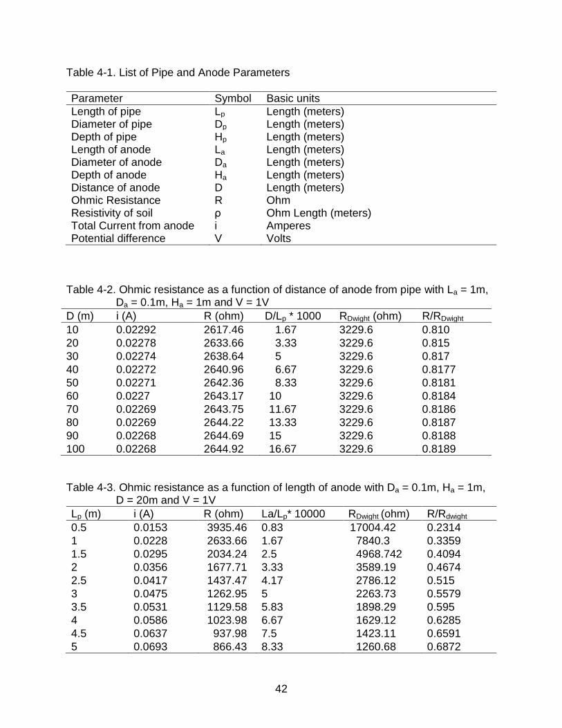
4-1 List of Pipe and Anode Parameters .................................................................... 42
4-2 Ohmic resistance as a function of distance of anode from pipe with La = 1m, Da = 0.1m, Ha = 1m and V = 1V .......................................................................... 42
4-3 Ohmic resistance as a function of length of anode with Da = 0.1m, Ha = 1m, D = 20m and V = 1V ........................................................................................... 42
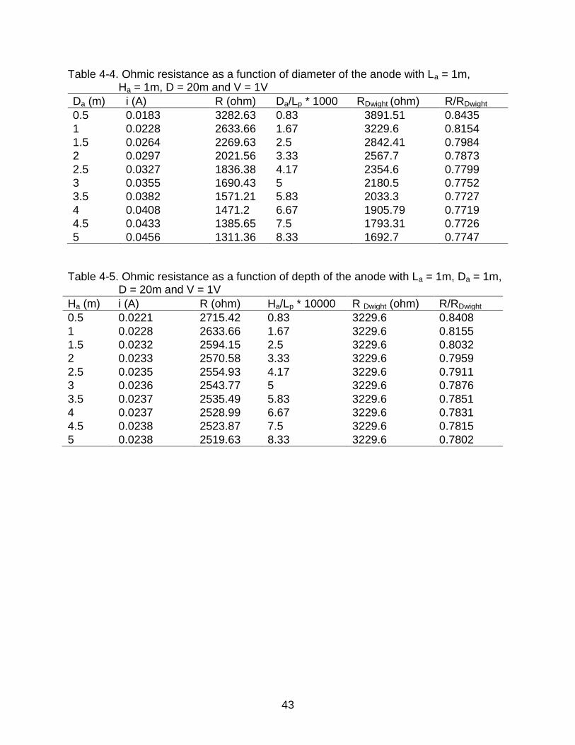
4-4 Ohmic resistance as a function of diameter of the anode with La = 1m, Ha = 1m, D = 20m and V = 1V ............................................................................ 43
4-5 Ohmic resistance as a function of depth of the anode with La = 1m, Da = 1m, D = 20m and V = 1V ........................................................................................... 43
4-6 Coating and Steel property parameters for the CP3D simulations ..................... 44
4-7 Simulation parameters ........................................................................................ 44
4-8 Anode parameters used in CP3D simulations .................................................... 44
4-9 Model parameters and result of single pipe configuration .................................. 45
4-10 Model parameters and result of two pipes single CP configuration .................... 45
4-11 Model parameters and result of two pipes with independent CP configuration .. 46
4-12 Model parameters and result of two pipes having independent CP with holiday on one pipe configuration ....................................................................... 46
4-13 Model Parameters and simulation results for tank bottoms with different coating properties ............................................................................................... 47
4-14 Non dimensional Current density as a function of non dimensional radius on tank bottoms with different coating properties .................................................... 48
4-15 Off Potential distribution as a function of non dimensional radius on tank bottoms with different coating properties ............................................................ 49
4-16 Model Parameters and simulation results for tank bottoms with different coating properties and holidays .......................................................................... 50
4-17 Current and On Potential distribution as a function of Distance along the Radius on tank bottoms with different coating properties and holidays .............. 51

8
A-1 Potential and Current Distribution on Pipe 1 Single pipe .................................... 72
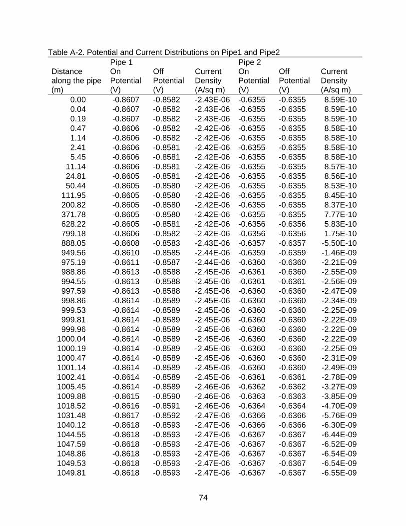
A-2 Potential and Current Distributions on Pipe1 and Pipe2 ..................................... 74
A-3 Potential and Current Distributions Pipe1 and Pipe2 .......................................... 76
A-4 Potential and Current Distributions on Pipe1 ...................................................... 79
A-5 Potential and Current Distribution on Pipe2 ........................................................ 81
9
LIST OF FIGURES
Figure page 4-1 Non Dimensional Ohmic resistance as a function of D with La, Da, Ha fixed ....... 52
4-2 R/RDwight as a function of Distance of anode with La, Da, Ha fixed ....................... 52
4-3 Non Dimensional Ohmic resistance as a function of Da with La, Da, D fixed ....... 52
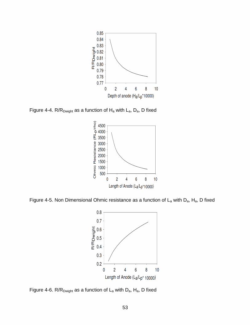
4-4 R/RDwight as a function of Ha with La, Da, D fixed ................................................. 53
4-5 Non Dimensional Ohmic resistance as a function of La with Da, Ha, D fixed ....... 53
4-6 R/RDwight as a function of La with Da, Ha, D fixed ................................................. 53
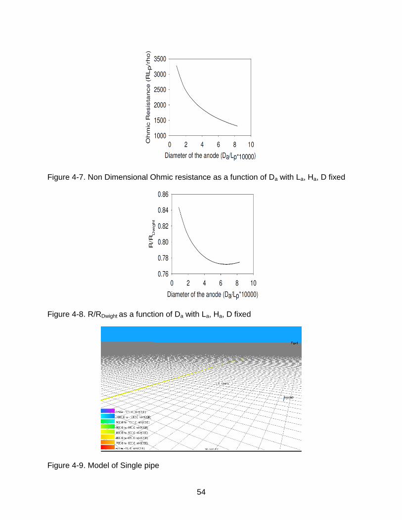
4-7 Non Dimensional Ohmic resistance as a function of Da with La, Ha, D fixed ....... 54
4-8 R/RDwight as a function of Da with La, Ha, D fixed.................................................. 54
4-9 Model of Single pipe ........................................................................................... 54
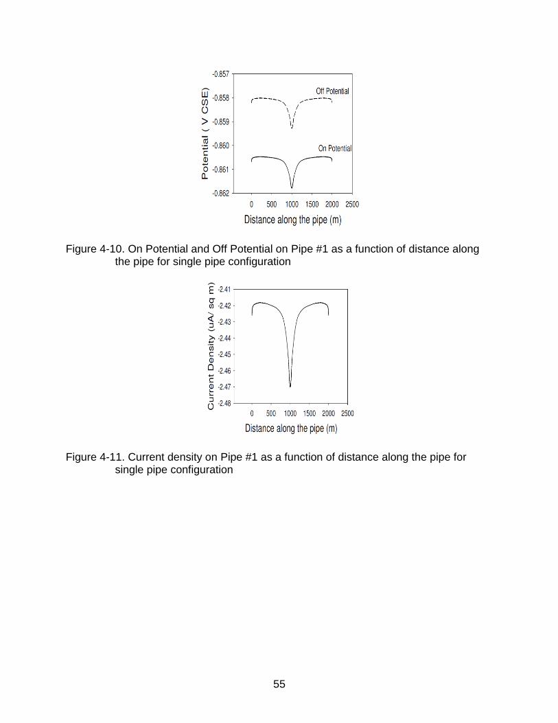
4-10 On Potential and Off Potential on Pipe #1 as a function of distance along the pipe for single pipe configuration ........................................................................ 55
4-11 Current density on Pipe #1 as a function of distance along the pipe for single pipe configuration ............................................................................................... 55
4-12 Model of two Pipes with Single CP ..................................................................... 56
4-13 On Potential and Off Potential on Pipe #1 as a function of distance along the pipe for two Pipes with Single CP configuration ................................................. 56
4-14 Current Density on Pipe #1 as a function of distance along the pipe for two Pipes with Single CP configuration ..................................................................... 57
4-15 On Potential and Off Potential on Pipe #2 as a function of distance along the pipe for two Pipes with Single CP configuration ................................................. 57
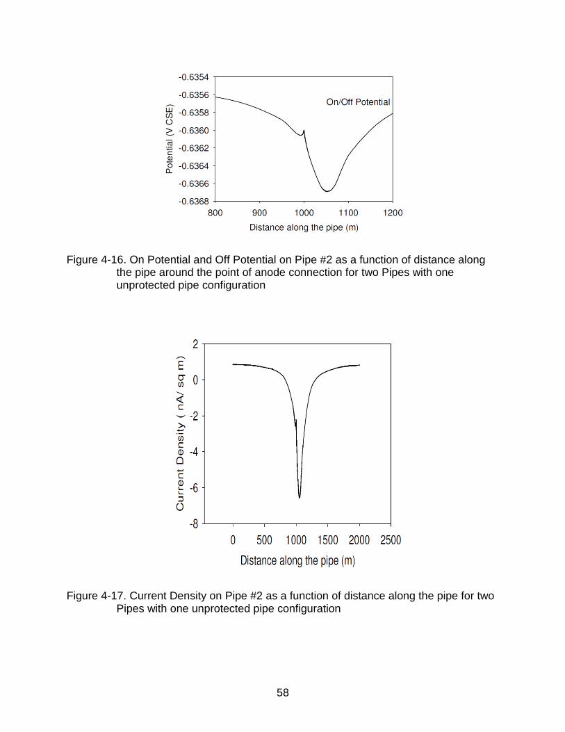
4-16 On Potential and Off Potential on Pipe #2 as a function of distance along the pipe around the point of anode connection for two Pipes with one unprotected pipe configuration ........................................................................... 58
4-17 Current Density on Pipe #2 as a function of distance along the pipe for two Pipes with one unprotected pipe configuration ................................................... 58
4-18 Current Density on Pipe #2 as a function of distance along the pipe around the point of anode connection for two Pipes with one unprotected pipe configuration ....................................................................................................... 59
10
4-19 Model of two pipes with independent Cp ............................................................ 59
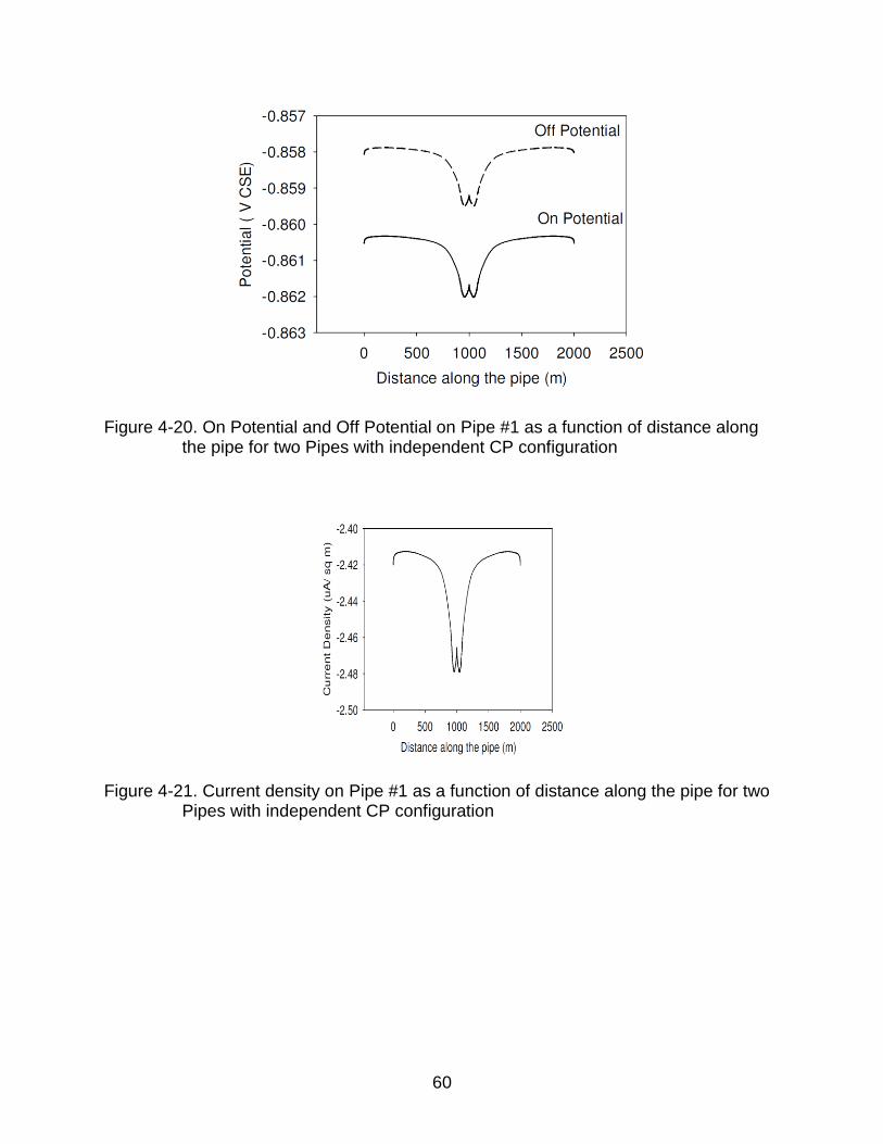
4-20 On Potential and Off Potential on Pipe #1 as a function of distance along the pipe for two Pipes with independent CP configuration ........................................ 60
4-21 Current density on Pipe #1 as a function of distance along the pipe for two Pipes with independent CP configuration ........................................................... 60
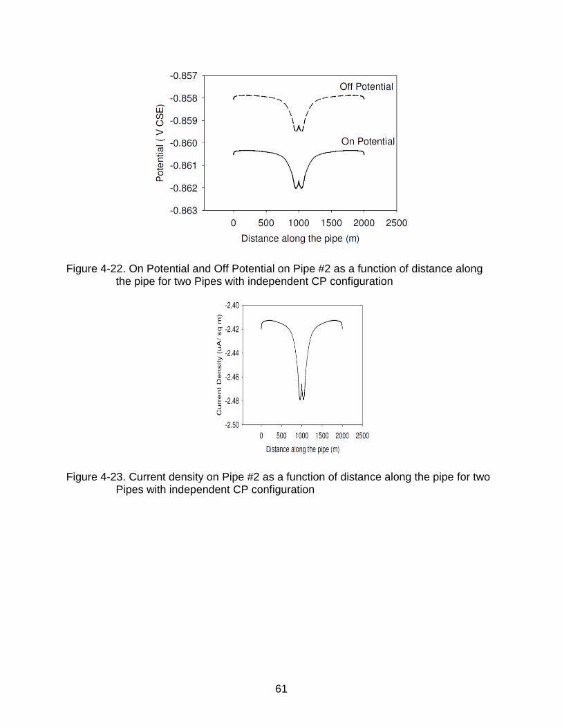
4-22 On Potential and Off Potential on Pipe #2 as a function of distance along the pipe for two Pipes with independent CP configuration ........................................ 61
4-23 Current density on Pipe #2 as a function of distance along the pipe for two Pipes with independent CP configuration ........................................................... 61
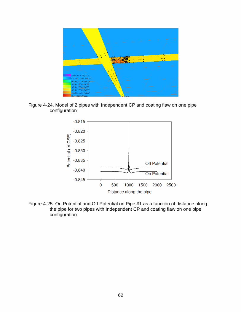
4-24 Model of 2 pipes with Independent CP and coating flaw on one pipe configuration ....................................................................................................... 62
4-25 On Potential and Off Potential on Pipe #1 as a function of distance along the pipe for two pipes with Independent CP and coating flaw on one pipe configuration ....................................................................................................... 62
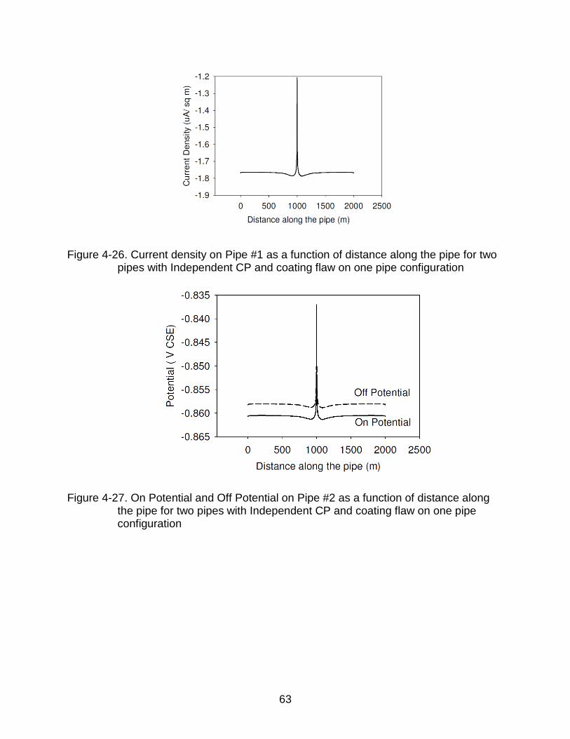
4-26 Current density on Pipe #1 as a function of distance along the pipe for two pipes with Independent CP and coating flaw on one pipe configuration ............. 63
4-27 On Potential and Off Potential on Pipe #2 as a function of distance along the pipe for two pipes with Independent CP and coating flaw on one pipe configuration ....................................................................................................... 63
4-28 Current density on Pipe #2 as a function of distance along the pipe for two pipes with Independent CP and coating flaw on one pipe configuration ............. 64
4-29 Steel A ................................................................................................................ 64
4-30 Steel B ................................................................................................................ 65
4-31 Coating A ............................................................................................................ 65
4-32 Coating B ............................................................................................................ 66
4-33 Non dimensional Current Density as a function of non dimensional radius on Tank Bottoms with different coating properties ................................................... 66
4-34 Off Potential as a function of non dimensional radius on Tank Bottoms with different coating properties ................................................................................. 67
4-35 Coating A with holiday exposing Steel B ............................................................ 67
4-36 Coating B with holiday exposing Steel B ............................................................ 68

11
4-37 Current Density as a function of Distance along the Radius on Tank Bottoms with different coating properties and holidays ..................................................... 68
4-38 On Potential as a function of Distance along the Radius on Tank Bottoms with different coating properties and holidays ..................................................... 69
12
Abstract of Thesis Presented to the Graduate School of the University of Florida in Partial Fulfillment of the Requirements for the Degree of Master of Science
CATHODIC PROTECTION MODELLING OF BURIED STRUCTURES
By
Alok Shankar
May 2012
Chair: Mark Orazem Major: Chemical Engineering
Petroleum products are of vital importance to the preservation of
industrial civilization. These products have been transported over long distances by
buried steel pipelines. The pipes are generally in soil environments which contain
oxygen and therefore can undergo corrosion. Over the past years, several accidents
have been reported which were caused by corrosion, resulting in loss of property and
life. These pipes are protected against corrosion using coating and cathodic protection
systems.
As the demand for petroleum has increased over the years, multiple pipelines
sharing rights of way have been used to transport the products. These products are
stored in large above ground storage tanks. As each structure is provided with
independent cathodic protection system, there arises the possibility of interaction
between the different CP systems installed. This interference can cause regions on the
structure to be either over or under protected. The effect is greater when there are
coating defects in the structures.
The objective of this work was to use CP3D, a numerical simulation tool, to study
the effect of interference in cathodic protection systems for pipelines. The calculated

13
potential and current distributions along the length of the structure were used to
understand the interference effect and performance of cathodic protection system. The
simulation tool was also used to extend the recent modeling studies of tank bottoms to
account for the presence of coatings and coating flaws on the ability of CP systems to
provide adequate protection.

14
CHAPTER 1 INTRODUCTION
Petroleum products are of vital importance to the preservation of
industrial civilization. These products have been transported over long distances by
buried steel pipelines. The pipes are present in soil environments which contain oxygen
and water. Therefore an unprotected pipe may undergo corrosion. Coatings are used as
primary protection for buried pipelines and cathodic protection installations are used as
secondary protection. Over the past years, several incidents have been reported which
were caused by corrosion or failure of protection systems, resulting in loss of property
and lives [1].
One such incident occurred in Plum Borough, Pennsylvania in 2008, where a
natural gas explosion destroyed a residence, killing a man and seriously injuring a 4-
year-old girl. Two other houses were destroyed, and 11 houses were damaged
amounting to property damage and losses worth a million dollars. The National
Transportation Safety Board determined that the probable cause of the leak and
explosion was excavation damage to the 2-inch natural gas distribution pipeline that
stripped the pipe’s protective coating and made the pipe susceptible to corrosion and
failure [2].
Direct currents are deliberately introduced into the earth to apply cathodic
protection to any buried structure. The current may damage other structures which are
present in the same earth. The corrosion engineer is responsible to prevent damage to
the underground structure. Cathodic interference is a more manageable problem than
stray current. A steady exposure exists hence more accurate measurements and
adjustments can be carried out. The source of current is under control and the rectifier

15
can be switched on and off when desired. When the magnitude of the current involved
is high, the exposure can be severe as all the current return is by the earth path than
just at the portion where leaks occur [3].
There are approximately 8.5 million regulated and non-regulated aboveground
storage tanks (ASTs) and underground storage tanks (USTs) for hazardous materials
(HAZMAT) in the United States.
The total cost of corrosion for storage tanks is estimated to be $7.0 billion per year
(ASTs and USTs). The cost of corrosion for all ASTs was estimated at $4.5 billion per
year. A vast majority of the ASTs are externally painted, which is a major cost factor for
the total cost of corrosion. In addition, approximately one-third of ASTs have cathodic
protection (CP) on the tank bottom, while approximately one-tenth of ASTs have internal
linings. These last two corrosion protection methods are applied to ensure the long-term
structural integrity of the ASTs [4].
Petroleum products are generally stored in a collection of aboveground storage
tanks called tank farms. These tanks are cylindrical, built from steel, and placed on the
soil. These tank bottoms are subjected to similar corrosion as the buried pipelines. The
tank bottoms are generally made of thinner metal than pipelines as it is supported by
ground and only subjected to hydrostatic pressures. The thinner metal is more easily
prone to even slow rates of corrosion. Hence, it is critical to provide cathodic protection
to tank bottoms which presents design challenges compared to buried pipelines [5].
The type of coating on the tank bottoms plays an important role in the performance
of cathodic protection system. It affects the distribution of the protection current when
different types of coatings exist.
16
Since the times cathodic protection was used, the engineers had to rely on
experience and intensive monitoring to optimize the design to prevent corrosion.[3] The
performance of the cathodic protection system depends crucially on the anode
parameters. The parameters such as distance of anode from the structure, the depth of
the anode, diameter and length of the anode play a major role in determining the extent
of protection of any buried structure. Wrong currents and positions can lead to
unprotected or over protected areas on the buried structures [6]

17
CHAPTER 2 LITERATURE REVIEW
Corrosion
Corrosion of metallic materials is classified into three groups.[7] The first
classification is wet Corrosion where the liquid electrolytes namely water with dissolved
species forms the corrosive environment. The second classification namely dry
corrosion also known as chemical corrosion comprises of dry gas as the corrosive
environment. The third classification is corrosion in other fluids such as fused salts and
molten metals. The current study is restricted to Wet corrosion of steel.
Electrode Kinetics
Iron corrosion has been described in two mechanisms depending on the pH. The
soil environment presents an alkaline environment for cathodic protection. [8] [9].
Under high pH values,
R.D.S- -
2Fe + 2 OH Fe(OH) + 2e (2-1)
2 -
2Fe(OH) Fe + 2OH (2-2)
where R.D.S. stands for Rate-Determining Step. The sum of reactions (2-1) and (2-2)
gives the net reaction which is an anodic reaction when the reaction proceeds from left
to right.
For iron deposition, the reactions are written as
2 -
2Fe(OH) Fe + 2OH (2-3)
-
2Fe(OH) + 2e Fe + 2OH (2-4)
where equation (2-4) represents the cathodic reactions from left to right.
18
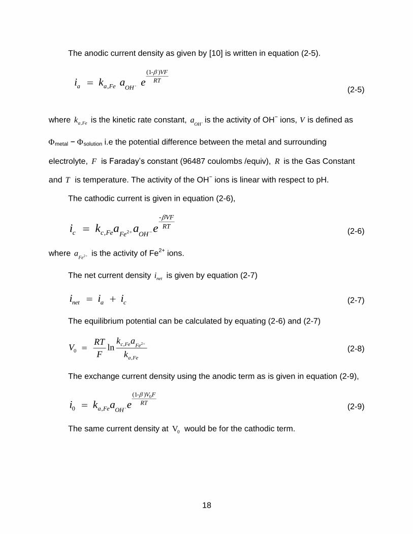
The anodic current density as given by [10] is written in equation (2-5).
-
(1- )
, VF
RTa a Fe OHi k a e
(2-5)
where ,a Fek is the kinetic rate constant, -OHa is the activity of OH− ions, V is defined as
metal − solution i.e the potential difference between the metal and surrounding
electrolyte, F is Faraday’s constant (96487 coulombs /equiv), R is the Gas Constant
and T is temperature. The activity of the OH− ions is linear with respect to pH.
The cathodic current is given in equation (2-6),
2
-
, VF
RTc c Fe Fe OHi k a a e
(2-6)
where 2Fea is the activity of Fe2+ ions.
The net current density neti is given by equation (2-7)
net a ci i i (2-7)
The equilibrium potential can be calculated by equating (2-6) and (2-7)
2,
0
,
ln c Fe Fe
a Fe
k aRTV
F k
(2-8)
The exchange current density using the anodic term as is given in equation (2-9),
0
-
(1- )
0 , V F
RTa Fe OH
i k a e
(2-9)
The same current density at 0V would be for the cathodic term.
19
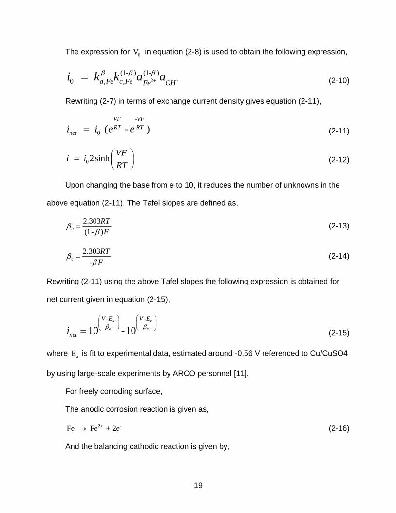
The expression for 0V in equation (2-8) is used to obtain the following expression,
2 -
(1- ) (1- )
0 , , a Fe c Fe Fe OHi k k a a
(2-10)
Rewriting (2-7) in terms of exchange current density gives equation (2-11),
-
0 ( - )VF VF
RT RTneti i e e (2-11)
0 2sinhVF
i iRT
(2-12)
Upon changing the base from e to 10, it reduces the number of unknowns in the
above equation (2-11). The Tafel slopes are defined as,
2.303
(1- )a
RT
F
(2-13)
2.303
-c
RT
F
(2-14)
Rewriting (2-11) using the above Tafel slopes the following expression is obtained for
net current given in equation (2-15),
- -
10 -10
a c
a c
V E V E
neti
(2-15)
where aE is fit to experimental data, estimated around -0.56 V referenced to Cu/CuSO4
by using large-scale experiments by ARCO personnel [11].
For freely corroding surface,
The anodic corrosion reaction is given as,
2 -Fe Fe + 2e (2-16)
And the balancing cathodic reaction is given by,
20
- -
2 2O + 2H O + 4e 4OH (2-17)
Equation (2-17) is known as the oxygen-reduction reaction. A Tafelian nature is
assumed for the rate of oxygen reaction. When a steel pipe is connected to another
active metal anode (Zn or Mg), a second cathodic reaction occurs. Also, the potential
shifts sufficiently negative.
- -
2 22H O + 4e H + 2OH (2-18)
The above reaction (2-18) is commonly known as the hydrogen evolution reaction.
Since the hydrogen evolution reaction follows Tafel kinetics, an equation similar to the
cathodic reaction is used [1].
Corrosion potential can be defined as the potential difference between a reference
electrode and a freely corroding surface. Corrosion potential is different from equilibrium
potential as more than one reaction takes place. It is a function of the oxygen content
and transport characteristics for oxygen within the electrolyte of the system.
The sum of the equations gives the total current which can be written as,
, ,
, ,
, ,2 2
, ,2 2
, ,2 2
, ,2 2
- -
- -
- -
10 -10
10 -10
10 -10
a Fe c Fe
a Fe c Fe
a O c O
a O c O
a H c H
a H c H
V E V E
total
V E V E
V E V E
i
(2-19)
The above equation can be further simplified by ignoring certain terms depending on the
potential range of interest. Upon setting the equation to zero and solving for V, we can
calculate the corrosion potential Vcorr. This is the same potential as the one measured
21
under zero current experimental condition. It is measured using a reference electrode
just outside the surface of the metal.
Application to Corrosion in Soil
When two different metals are interconnected in soil, one metal will corrode at a
higher rate than it would independently and the other would corrode at a lower rate. This
can be used as boundary condition in a numerical method considering that the kinetics
is known. A mass transfer limited reaction would exist as the reactant comes from the
electrolyte. The equation (2-20) can be used to describe the kinetics at the boundary. In
a steady state soil system as discussed in [12] bare steel takes the form,
2
2
2
2
2
- ( - - ) - -
- -
lim
1 10 - - 10
1 - 10
HFe
HFe
O
O
V EV E
soil V E
O
i
i
(2-20)
where 2limOi is the mass transfer limited current density for oxygen reduction. It is
termed as limiting as part of the current due to oxygen reduction cannot exceed the
value of 2limOi .
Since it is assumed that sufficient water is always available around the pipe in soil
environment, no limitation is observed for hydrogen evolution reaction to proceed under
kinetic limitation.
Corrosion Prevention Methods
Several measures can be implemented for removing or reducing the effect of the
conditions that leads to corrosion [7]. One way is to select a material does not corrode
in the actual environment. The surrounding environment can be changed, e.g. we can
22
remove oxygen from the environment or add anti corrosion chemical behaving as
inhibitors. Other method is incorporating design modifications which avoid corrosion.
The potential of the metal surface can be changed to a more negative value. Coatings
can be applied to provide a barrier for the metal against the corrosive environment.
Cathodic Protection
The technique where an undesired reaction is replaced by a more desired reaction
on a given metal surface is known as cathodic protection. For example the undesired
reaction for buried metallic structure is the dissolution of metal.
The principle of cathodic protection is to have a secondary surface within the
conductive soil at a more negative potential than the pipe steel. The pipe steel is
connected to this surface with a wire [1].
The cathodic protection in general practice is coupled with coatings to protect the
areas of defected coating or holidays from corrosion. The coating forms the primary
form of protection. Cathodic protection installations can be used for buried metallic
pipelines, buried tanks, other offshore structures [7].
The theoretical basis of cathodic protection is provided by an Evans diagram. The
activation process controls the metal dissolution reaction. The cathodic reaction
diffusion is limited at higher density. When we increase the cathodic current density, the
potential of the metal decreases and the anodic dissolution rate reduces. Since
logarithmic scales are used for current, for each unit in decrease of metal potential, the
current requirements increase exponentially. [3]
Criterion for Cathodic Protection
The cathodic protection to be applied to a given structure depends on the material
of the structure to be protected, the environment of the structure, the level of protection
23
required, the potential at the electrolyte interface and the non uniform corrosion
potentials of the corroding structures.
If the level of protection is too little then excessive corrosion can take place, on the
other hand excessive current can cause disbonding of the coatings.
For a buried steel structure, the potential criteria proposed are:
Potential of the structure with respect to saturated Cu/CuSO4 is -850mV under aerobic conditions. This is the most widely used criterion as it is easy to employ.
-300 mV negative potential shift is observed when current is applied.
Since protection criteria is dependent on the potential of the structure at the soil
interface, corrections have to be incorporated to the measurements performed when
reference electrode is placed some distance away from the structure. The
measurements are thus carried out in ON and OFF condition of the CP system to satisfy
the potential shift criteria. [3]
Anode Polarization
The typical anodes used in cathodic protection are Galvanic or Sacrificial anodes
and impressed current anodes. These undergo a similar electrochemical process as the
buried structure like pipes or tank bottoms. The corrosion term comprises of an
oxidation-reduction reaction but the interest lies in corrosion (oxidation) of the anode
material.
Galvanic Anodes
These types of anodes are more active than the metal of the structure that needs
to be protected. Typical galvanic anodes used in soil environment are carbon steel, zinc
and magnesium. These have large driving forces in the highly resistive soil environment
to provide protection. [7]
24
The galvanic anode model is described as
2
- -
10 - 1
corr
anode
V E
galvanic Oi i
(2-21)
Where galvanici is current due to galvanic anode, 2Oi is the mass-transfer-limited current
density for oxygen reduction, V is the voltage of the anode, is the voltage just
outside the surface of the anode, corrE is the free corrosion (equilibrium) potential of the
anode and anodeβ is the Tafel slope for the anode corrosion reaction. The three
parameters of the model are generally known for all types of galvanic anodes. The
contribution of the hydrogen reaction is small at the typical operating potentials and
hence ignored [1].
Since the driving force for reduction reaction is always higher than freely corroding
steel, the operating conditions typically ensure that the reduction is always mass
transfer limit. Thus, a constant term is assumed.
Impressed Current Anodes
Impressed current cathodic protection is applied through an external power current
source. Usually, the outside current source is a rectifier which provides the activity. The
orders of current densities and power output range on impressed current anodes are
usually higher than that of galvanic anodes thus greater driving force. The numbers of
anodes required are fewer even in highly resistive environments. Larger areas can be
protected using the impressed current cathodic protection system. They provide the
user the ability to adjust the protection levels. The anode consumption levels are usually
much lower than galvanic anodes and hence the system has a longer life.[3]
25
A dimensionally stable anode connected to the positive terminal of a direct current
source is the set up of an impressed current system. The pipe is connected to the
negative terminal of the DC source.
The most probable reactions of ICCP system are water oxidation and chloride
oxidation as the anodes do not react [1].
+ -
2 22H O O + 4H + 4e (2-22)
- -
22Cl Cl + 2e (2-23)
The impressed current anode model is given as,
2 - - -
10 - 1
rectifier O
anode
V V E
ICCPi
(2-24)
where ICCPi is current density in ICCP anode, an additional term rectifierV is added to the
exponent to account for the potential setting of the rectifier, V is the voltage of the
anode, is the voltage just outside the surface of the anode, 2OE is the equilibrium
potential for the oxygen evolution reaction, and anode is the Tafel slope for the oxygen
evolution reaction.
Tank Bottoms
Cathodic protection of storage tanks against external corrosion requires good
coating and low protection current density. Effective cathodic protection with small
protection current densities can be achieved with new installations. For older tanks,
larger current densities are required. It also depends on the coating and the state of the

26
tanks. The cost for protective installations and work is generally higher for older tank
installations [5].
The criterion for protection used for tank bottoms are similar to the ones used for
pipelines where oxygen reduction is assumed to be the standard cathodic reaction on
the tank bottoms.
The circular area of a tank bottom has inherent non uniform current distribution.
This leads to a compromise in the delivery of protection current to the center of the tank.
A more uniform behavior can be observed if certain limitations to the kinetics and mass
transfer are applied [5].

27
Table 2-1. Parameters for the oxygen and chlorine evolution reactions [13]
Reaction Equilibrium Potential (E), mV (CSE)
Tafel Slope (β), mV/decade
O2 evolution -172 100 Cl2 evolution 50 100

28
CHAPTER 3 CATHODIC PROTECTION 3-D MODELLING SOFTWARE
CP3D is a complex, powerful, and computationally intensive piece of modeling
software. The prediction of the performance of cathodic protection systems under
conditions like modern use of coatings, localized failure of pipes at discrete coating
defects requires a mathematical model that can account for current and potential
distributions in both angular and axial directions. This model accounts for current flow in
the soil, pipes and the circuitry. Long pipes exhibit non negligible potential difference
along the steel [1].
The current software accounts for the flow of current through two separate
domains. The first is the soil domain enclosed by the pipes and anodes surfaces,
interface between soil and air and interface between soil and any buried surfaces if any.
The second domain contains the metallic wall of the pipe, the volume of the anode and
connecting wires and resistors for the return of the protective current. These domains
are electrochemically linked.
Soil Domain
This domain contains the material in which the pipes and anodes are buried. It
does not comprise the interior volume of the pipeline steel. The concentrations and
potential within the soil needs a solution of a coupled set of equations, including
conservation of each individual solute species [10]. The material balance equation over
a small volume element is given in equation (3-1).
( . )i i
cN R
t
(3-1)

29
and electroneutrality expression is given as,
0i i
i
z c (3-2)
where ic is the concentration of species i, iR is the rate of generation of species i due to
homogeneous reactions, and iN is the net flux vector for species i. In a dilute
electrolytic solution, the contributions to the flux iN are from convection, diffusion, and
migration. Under the assumption that soil represents a dilute solution, the flux is
given as
i iz ci i i
FN vc D c
RT
(3-3)
where v is the fluid velocity, iD is the diffusion coefficient for species i, iz is the charge
associated with species i, F is Faraday’s constant, and is the potential. Under the
assumption of a steady-state and a uniform concentration of ionic species, the current
density, expressed in terms of contributions from the motion of each ionic species, can
be given in terms of potential by Ohm’s law. The mobility is related to the diffusion
coefficient by the Nerst-Einstein equation.
i iD RTu (3-4)
The current current density is given by equation (3-5).
i i i
i
F z N (3-5)
where the conductivity , in terms of individual species contributions is expressed as
2 2
i i i
i
F z u c (3-6)

30
The conductivity has a uniform value because the concentration is uniform. The
assumption that concentrations are uniform yields Laplace equation given by equation
(3-7).
2 0 (3-7)
This is commonly used in cathodic protection models. The uniform concentration
assumption means that the gradients in concentration that are associated with pipeline
and anode surface reactions are assumed to occur within a thin layer adjacent to the
pipe and anode surfaces. This gradient in concentration within the narrow layer is
incorporated into the boundary condition which describes the electrochemical reactions.
Pipe or Inner Domain
When we consider long pipelines and large current levels, the potential drop in the
pipelines is significant [14].The flow of current through the pipe steel, anodes, and
connecting wires is strictly governed by the Laplace’s equation.
.( ) 0V (3-8)
where V is the departure of the potential of the metal from a uniform value and is the
material conductivity. The conductivity of the pipe-metal domain is not necessarily
uniform. A simplified version of Laplace equation given by equation (3-9)
ww
w
LV IR I
A (3-9)
can be used to account for the potential drop across connecting wires, where wR is the
resistance of the wire, is the electrical resistivity, wL is the length of the wire, and wA
is the cross-sectional area of wire.
31
Domain Coupling
The inner and outer domains described in sections 3.1 and 3.2, respectively, are
linked by boundary conditions where the current density on metal surfaces is related to
values of local potential. The type of surface governs the specific form of the
relationship required like bare steel, coated steel, galvanic anodes, and impressed
current anodes have been discussed earlier [1].
Numerical Development
Laplace’s equation has been solved for many boundary conditions and domains.
The software can be used to solve this equation for arbitrary arrangements of pipes and
anodes within the domain and the nonlinear boundary conditions that arise from the
chemistry at the boundaries as discussed earlier [1].
For corrosion problems where the activity is observed at the boundaries, the
boundary element numerical technique is used for solving governing equation at the
boundaries in soil domain.
The finite element method is used to solve the pipe steel domain. The solutions for
the current and potential distributions are available around the circumference and along
the length of the pipe. The domain is divided into elements using piecewise continuous
polynomial isoparametric shape functions. A special type of thin shell elements is
introduced here which are specifically designed for potential problems on shells where
the material’s absolute property, is large.
The pipe and anode are electrically connected using bonds and resistors. These
go from connection node on one pipe to connection node on another pipe. Thus, no
extra nodes are introduced. The resistor if specified within the wire, its resistance is
added to the total resistance of the bond. The boundary element domain and finite

32
element domain are coupled at the interface between the two domains where the Ohm’s
Law is valid within either domain.
33
CHAPTER 4 RESULTS AND DISCUSSION
The following section covers the effect of anode parameters on the performance of
cathodic protection systems, the interaction between the cathodic protection systems in
pipelines in cross over configuration, and effect of coatings on the protection current in
tank bottoms.
Dimensional Analysis of Anode Parameters
The current density is highest at the anode. It is important to understand the effect
of anode parameters on the performance of cathodic protection systems. The primary
current distribution was used to calculate Ohmic resistance. The anode parameters are
then validated using the Ohmic resistances.
The Buckingham pi method is used to find the relation between non dimensional
parameters as given in Table 4-1.
The relation obtained is
, , , p a a a
p p p p
RL D H L Df
L L L L
(4-1)
Theoretically, the resistance at the anode is calculated using the Dwight’s formula
80.005 ln - 1
p
Dwight
p p
LR
L D
(4-2)
The resistances were then compared to understand the effect of the anode parameters
and determine the dominant ones.
A pipe, 6 km long, 300 mm diameter at 1 m depth having equipotential surface
connected to an equipotential anode of different length, diameter buried at different
depths in soil having 10,000 ohm cm resistivity was modeled using CP3D software to
34
understand the effect of primary current distribution and the associated Ohmic
resistance on parameters associated with anode.
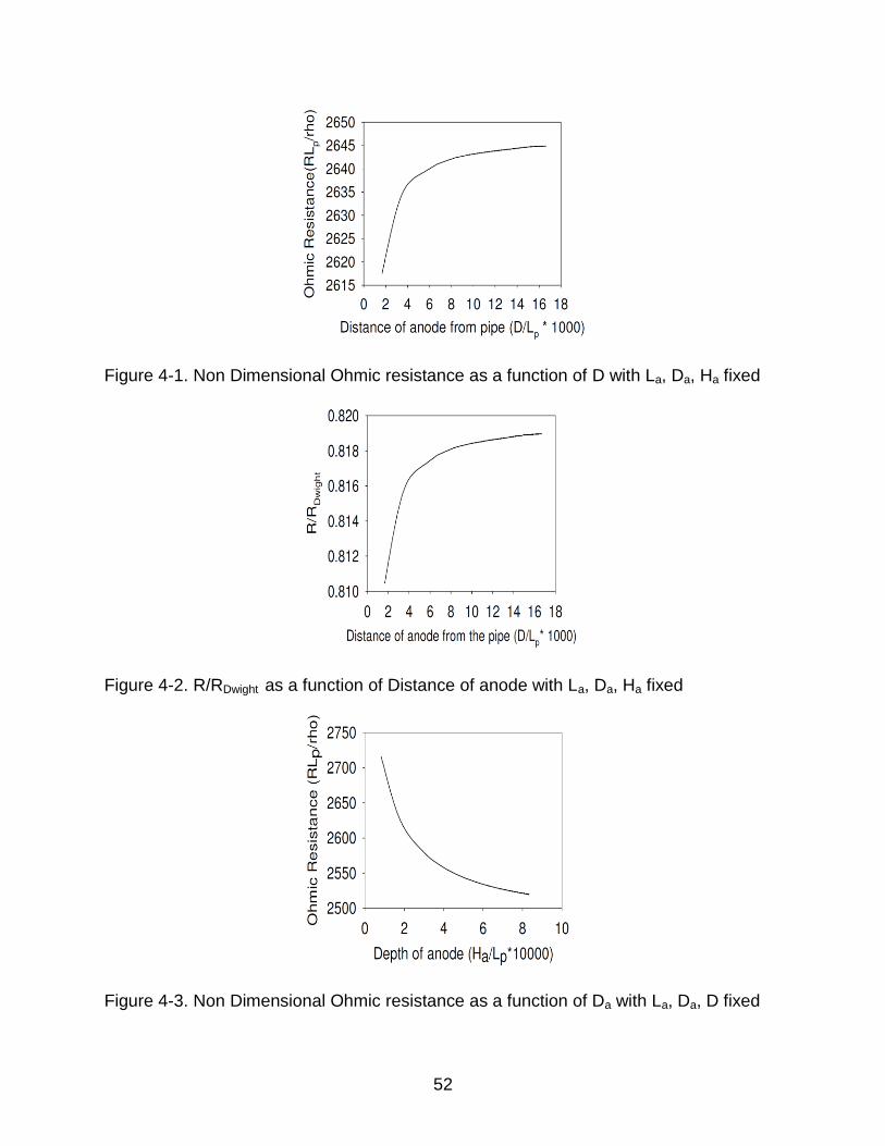
Influence of Anode Distance from Pipe
The variation of Ohmic resistance with distance of the anode from the pipe was
studied. The simulations resulted in slight variations of Ohmic resistance with distance
of anode from the pipe as seen in Figure 4-1. The resistance increased due to the
increase in soil section as the distance of the anode from the pipe increased. The
current density was highest near the anode and it reduced as distance from the anode
increased. Hence, for an equipotential anode, the change in resistance was observed to
be steeper near the anode than away from it.
The resistance measured using the simulation software was compared with the
Dwight resistance at the anode as shown in Figure 4-2. Better agreement between the
resistances was observed as the distance of the anode from the pipe was increased but
complete agreement was not seen as the Dwight resistance assumes that the anode is
placed infinitely away from the cathode where as in the simulation the cathode (pipe) is
located at a finite distance from the anode.
Influence of Anode Depth
The variation of Ohmic resistance with depth of the anode from the pipe was
studied. The simulations resulted in considerable variations of Ohmic resistance with
depth of the anode as shown in Figure 4-3. The amount of current at the anode would
be larger upon increasing the depth of the anode. As the depth of anode was increased,
greater section of soil is available for current to flow through the soil. Hence, for an
equipotential anode, the resistance decreased as we increased the depth of the anode.

35
The resistance measured using the simulation software was compared with the
Dwight resistance at the anode as shown in Figure 4-4. It was observed that the
agreement between the resistances decreased as the depth of the anode was
increased but complete agreement is not observed as the Dwight resistance does not
take into account the depth of the anode.
Influence of Anode Length
The variation of Ohmic resistance with length of the anode from the pipe was
studied. The simulations resulted in large variations of Ohmic resistance with increase
in the length of anode as shown in Figure 4-5. The amount of current at the anode
would be larger upon increasing the length of the anode. Hence, for an equipotential
anode, the Ohmic resistance measured at the anode decreased as the length of the
anode was increased.
Upon comparing the simulation resistance with the Dwight resistance as given in
Figure 4-6, it was observed that there was no complete agreement between the values
as the Dwight resistance does not account for the finite distance of the anode from the
cathode (pipe) and the depth of the anode.
Influence of Anode Diameter
The variation of Ohmic resistance with diameter of the anode was studied. The
simulations resulted in large variations of Ohmic resistance with increase in the
diameter of anode as shown in Figure 4-7. The amount of current at the anode would be
larger upon increasing the diameter of the anode. Hence, for an equipotential anode,
the Ohmic resistance measured at the anode decreases as the diameter of the anode is
increased.
36
Upon comparing the simulation resistance with the Dwight resistance given by
Figure 4-8, it is observed that there is no complete agreement between the values as
the Dwight resistance does not account for the finite distance of the anode from the
cathode (pipe) and the depth of the anode.
Cathodic Interference in Pipelines
The following section describes the different cases where interaction between the
cathodic protection installations for two pipelines in a cross over configuration was
observed.
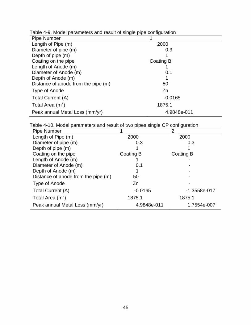
Base Case: Single Pipe
A single pipe, 2 km long, buried in the soil of resistivity 10000 ohm cm, connected
to a zinc anode at a certain distance was modeled using CP3D software as shown in
Figure 4-9.The model parameters are given in Table 4-9. The potential distribution
along the length of the pipe was observed to be uniform and in the protected range of
potentials as shown in Figure 4-10. The current density distribution along the length of
the pipe was cathodic and uniform shown in Figure 4-11. At the drainage point where
the anode was connected to the pipe, a more cathodic behavior was observed.
Two Pipes in Cross Over Configuration
Two pipes of equal dimensions and same coating properties were modeled in a
cross over configuration to understand the effect of interaction between different CP
systems installed on the respective pipelines.
One pipe unprotected
Two pipes of equal dimensions and same coating properties were modeled in a
cross over configuration as shown in Figure 4-12. The model parameters are given in
Table 4-10. A cathodic protection system was connected only to one of the pipes. The
37
potential and current distributions on the pipe with the CP system installed showed
same behavior as the single pipe without the effect of the new pipe introduced. The
potential and current distributions were uniform along the length of the pipe and in the
protection range as shown by Figure 4-13 and Figure 4-14 respectively.
The potential distribution on pipe which does not have a CP system installed was
outside the protection range but nearly uniform along the length of the pipe as shown in
Figure 4-16. At the cross over region, a minor peak in the potential and current
distributions was observed as shown in Figure 4-17 and Figure 4-18 respectively. This
is attributed to minor anodic potential and associated anodic current on the pipe. As a
result, localized corrosion can be observed at the cross over location.
Both pipes protected with independent CP
Two pipes of same dimensions and coating properties; each having independent
CP system installed was modeled to understand the interaction between CP systems as
shown in Figure 4-19. The model parameters are given in Table 4-11. The potential and
current distributions on both the pipes were in the protected range as shown in Figure 4-
20 and Figure 4-21 respectively. On pipe #1 two dips were observed in the potential and
current distributions. One dip is associated with the drainage point where the CP system
is connected to the pipe #1. The other dip is the associated with the CP connected to
the pipe #2 which are affecting the potential distribution on pipe #1. This is indicative of
interaction between the two CP systems. Similar behavior was observed in pipe #2 as
well where the CP of pipe #1 is affecting the distributions on pipe #2 as shown in Figure
4-22 and Figure 4-23.
38
Both pipes with independent CP systems and holiday on one pipe
The two pipe system in cross over configuration with a coating flaw on pipe #1 was
modeled to understand the effect of interaction between CP systems as shown in Figure
4-24. The model parameters are given in Table 4-12. The specifications of the holiday
are described in Table 4-12. The potential distribution on pipe #1 was observed to be
non uniform. More positive potential was observed at the site where coating flaw is
present as given in Figure 4-25. An anodic current as shown in Figure 4-26 is
associated at the site of coating flaw indicating that this location is most prone to
corrosion. Anodes with larger driving force should be used to ensure that the potentials
are in the protected range along the entire length of the pipe.
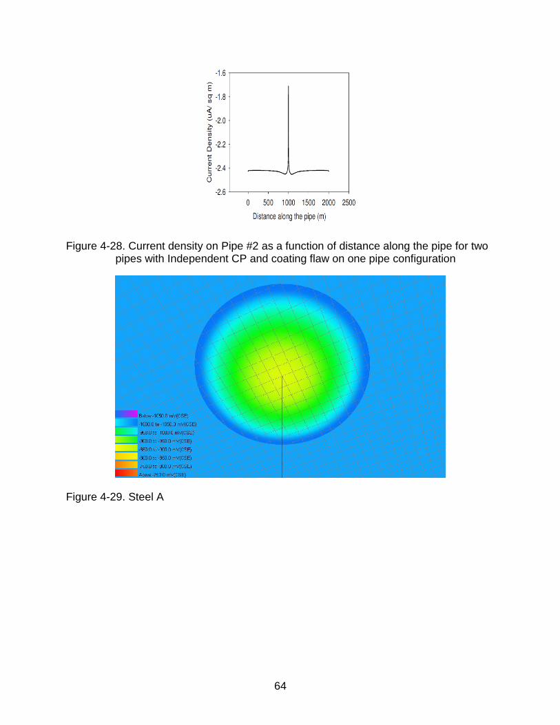
The potential distribution on pipe #2 is non uniform. A sharp positive peak in the
potential distribution is observed at the site where the coating flaw is present on pipe #1
as shown in Figure 4-27. An anodic current is associated at the same location indicating
that localized corrosion is possible at this location despite the absence of coating defect
on pipe #2 as shown in Figure 4-28. This behavior can be attributed to the possible
interaction between the 2 CP systems installed.
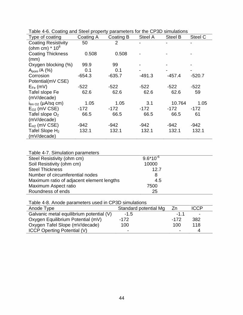
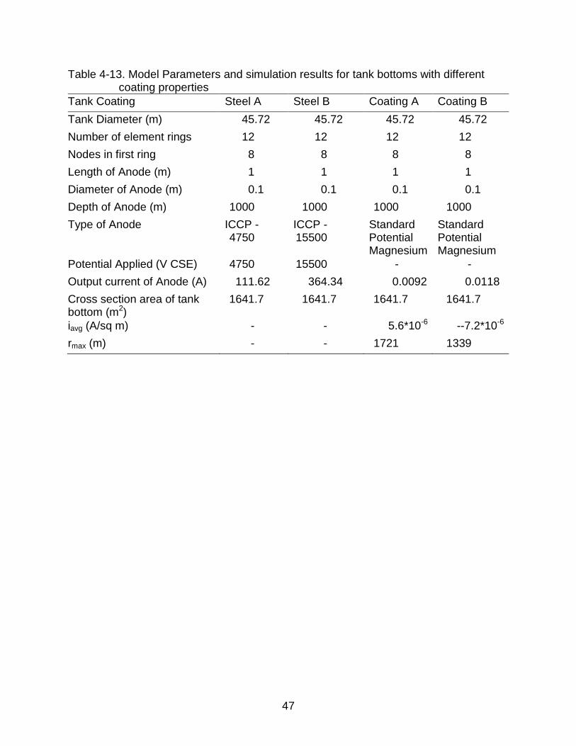
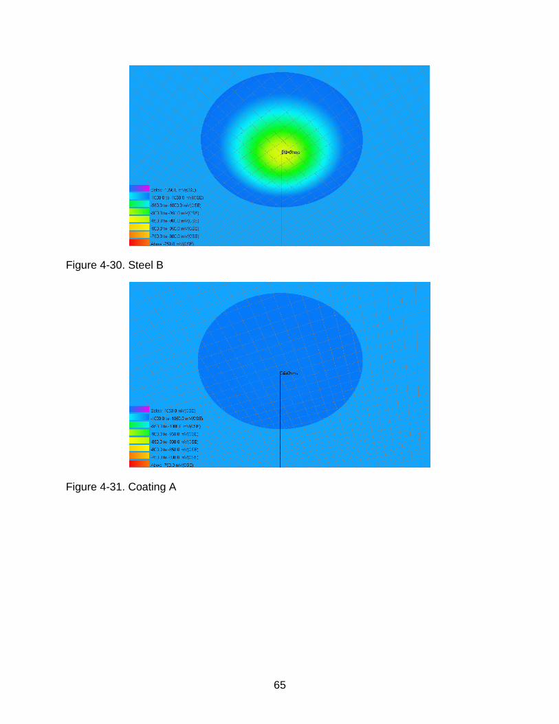
Effect of Coating on CP in Tank Bottoms
Tank bottoms with bare steel properties and different coatings connected to anode
located far away were modeled to understand the effect of coating properties on tank
bottoms. Four configurations were studied namely Steel A, Steel B, Coating A and
Coating B in a soil of uniform resistivity of 10000 ohm cm as shown in Figure 4-29,
Figure 4-30, Figure 4-31 and Figure 4-32 respectively. The model parameters and
anode specifications are given in Table 4-13. The protection current density as a
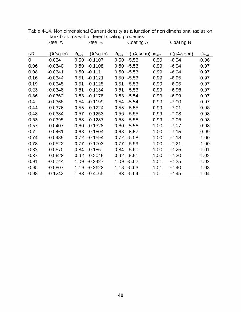
function of non dimensional radius is as shown in Figure 4-33.
39
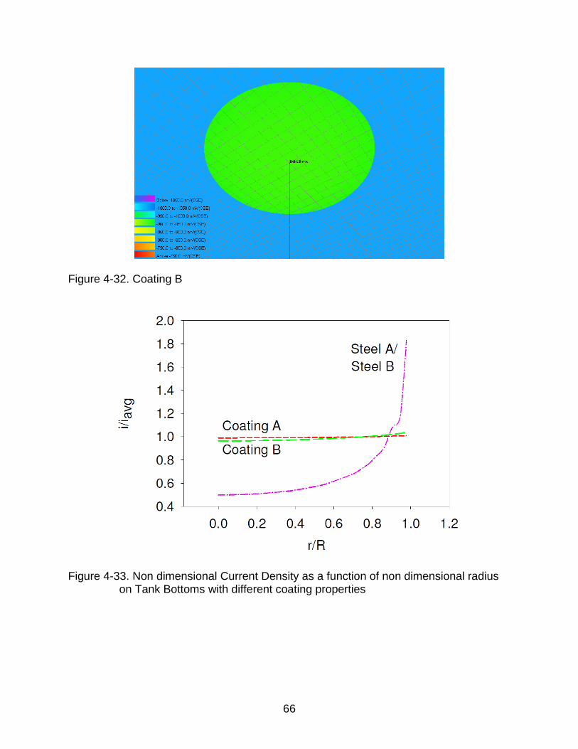
Riemer and Orazem[1] had reported that a tank bottom with no coatings cannot
be protected by a deep well remote ground bed when the output of the anode is 14.2
Amperes and anode is placed 250 feet from the tank bottom. In the case of Steel A and
Steel B where no coatings are present, the protection current distribution is observed to
be non uniform with the outer most ring having higher current density than the middle of
the tank bottom. This behavior is seen when Tafel kinetics apply where the corrosion
and hydrogen evolution play a role. The center of the tank was poorly polarized as the
net current density would be below the mass transfer limited current density for oxygen
reaction.
Upon increasing the applied potential to a larger value, the output current from the
anode also increased as shown in Table 4-12. The current distribution was observed to
be non uniform as the earlier result but the potential distribution in the tank bottoms
were observed to be in the protected range. The center of the tank had a potential of -
870 mV CSE and the outermost ring had a potential of -1065 mV CSE. The increased
net current is now above the mass transfer limited current density for oxygen reaction
and hence the tank bottom with no coatings was protected.
When we apply coatings in the tank bottoms, a near uniform current density was
observed along the radius of the tank bottom. The protection current required for coated
tank bottoms was lesser than in the case of tank bottoms with no coatings as a
reduction in transport of oxygen through a uniform barrier is seen. The potentials along
the radius are observed to be in the protection range as shown in Figure 4-34. The
uniform current density distribution helps in CP design where the maximum radius that
40
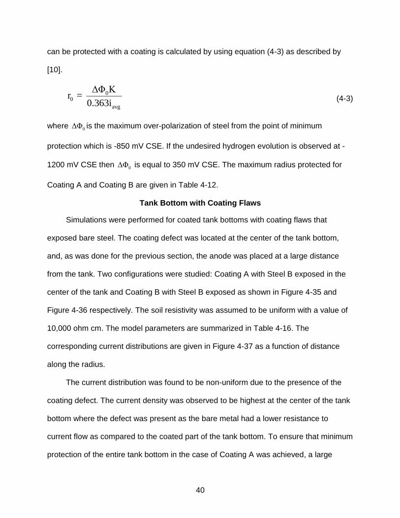
can be protected with a coating is calculated by using equation (4-3) as described by
[10].
00
avg
ΔΦ Κr =
0.363i
(4-3)
where 0ΔΦ is the maximum over-polarization of steel from the point of minimum
protection which is -850 mV CSE. If the undesired hydrogen evolution is observed at -
1200 mV CSE then 0ΔΦ is equal to 350 mV CSE. The maximum radius protected for
Coating A and Coating B are given in Table 4-12.
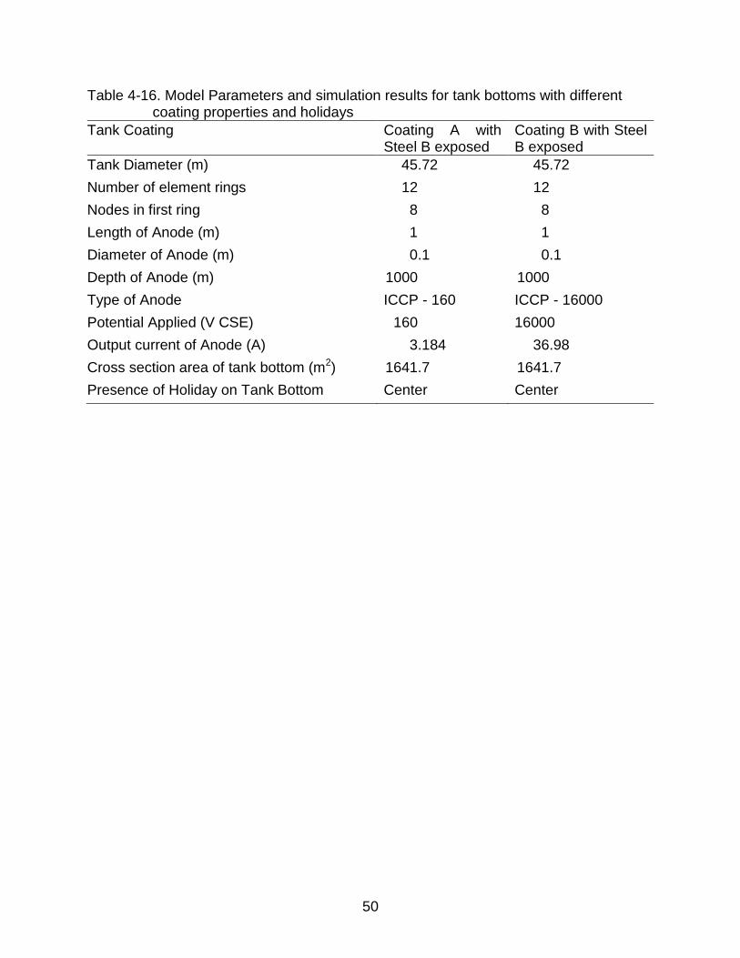
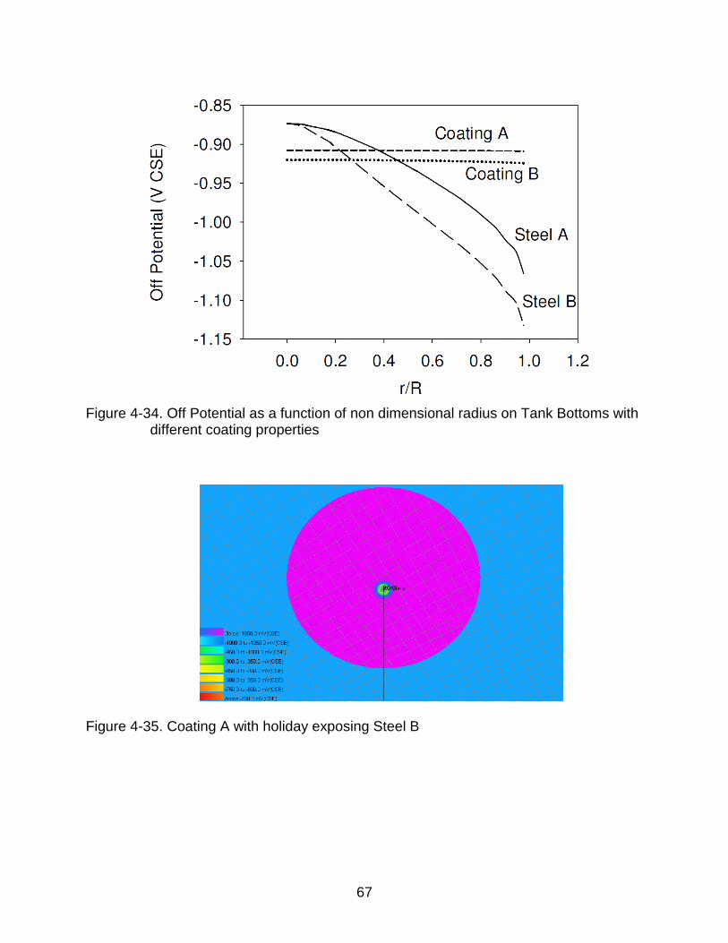
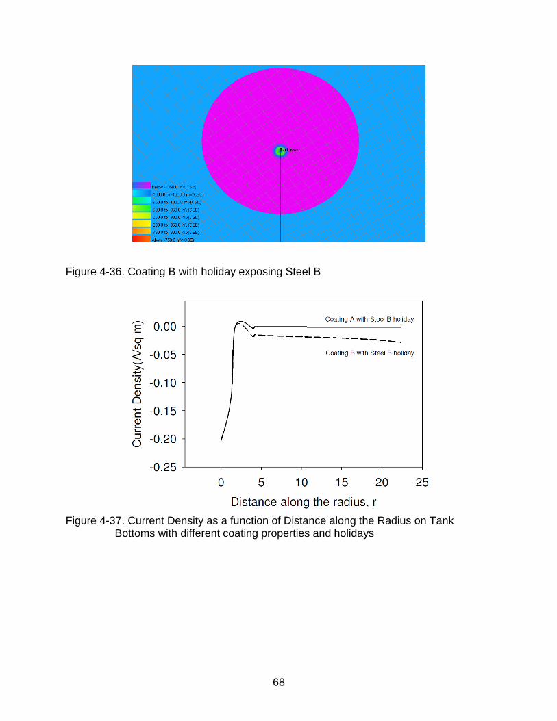
Tank Bottom with Coating Flaws
Simulations were performed for coated tank bottoms with coating flaws that
exposed bare steel. The coating defect was located at the center of the tank bottom,
and, as was done for the previous section, the anode was placed at a large distance
from the tank. Two configurations were studied: Coating A with Steel B exposed in the
center of the tank and Coating B with Steel B exposed as shown in Figure 4-35 and
Figure 4-36 respectively. The soil resistivity was assumed to be uniform with a value of
10,000 ohm cm. The model parameters are summarized in Table 4-16. The
corresponding current distributions are given in Figure 4-37 as a function of distance
along the radius.
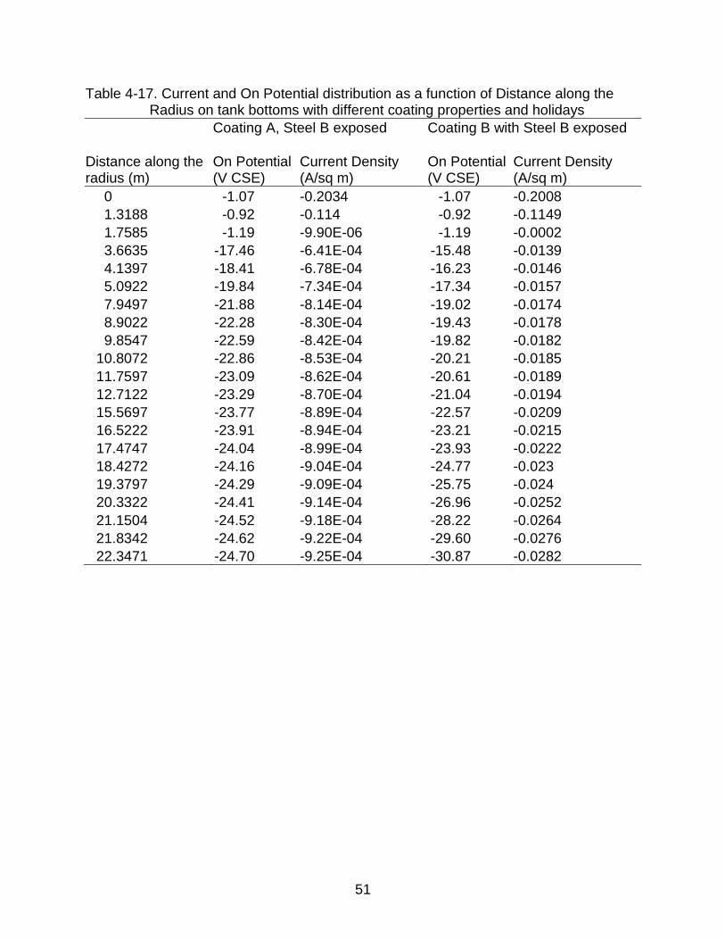
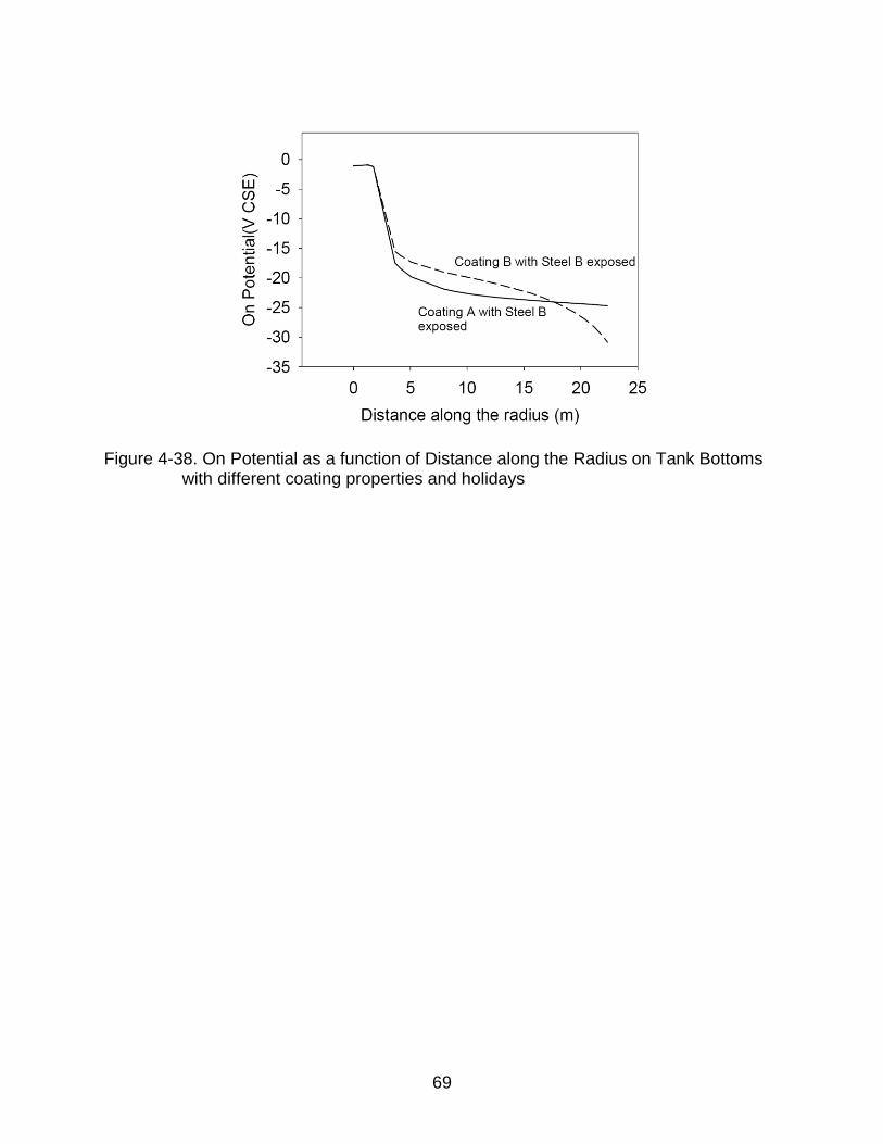
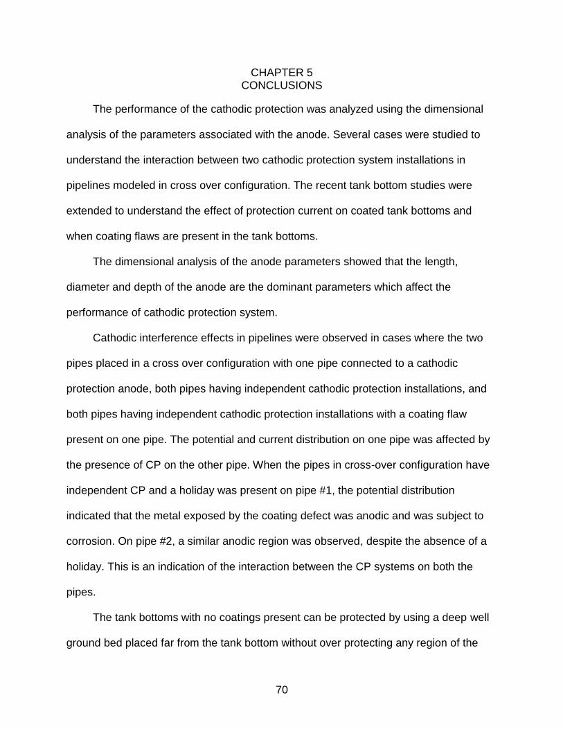
The current distribution was found to be non-uniform due to the presence of the
coating defect. The current density was observed to be highest at the center of the tank
bottom where the defect was present as the bare metal had a lower resistance to
current flow as compared to the coated part of the tank bottom. To ensure that minimum
protection of the entire tank bottom in the case of Coating A was achieved, a large

41
potential of 160V had to be applied. This resulted in large areas of tank bottom being
over protected as shown by the potential values in Table 4-17. In the case of Coating B,
a larger potential of 1600 V was applied to ensure minimum protection was achieved of
the tank bottom. This also resulted in large areas of the tank bottom being over
protected as shown by the potential distribution in Figure 4-38.
42
Table 4-1. List of Pipe and Anode Parameters
Parameter Symbol Basic units
Length of pipe Lp Length (meters) Diameter of pipe Dp Length (meters) Depth of pipe Hp Length (meters) Length of anode La Length (meters) Diameter of anode Da Length (meters) Depth of anode Ha Length (meters) Distance of anode D Length (meters) Ohmic Resistance R Ohm Resistivity of soil ρ Ohm Length (meters) Total Current from anode i Amperes Potential difference V Volts
Table 4-2. Ohmic resistance as a function of distance of anode from pipe with La = 1m, Da = 0.1m, Ha = 1m and V = 1V
D (m) i (A) R (ohm) D/Lp * 1000 RDwight (ohm) R/RDwight
10 0.02292 2617.46 1.67 3229.6 0.810
20 0.02278 2633.66 3.33 3229.6 0.815
30 0.02274 2638.64 5 3229.6 0.817
40 0.02272 2640.96 6.67 3229.6 0.8177
50 0.02271 2642.36 8.33 3229.6 0.8181
60 0.0227 2643.17 10 3229.6 0.8184
70 0.02269 2643.75 11.67 3229.6 0.8186
80 0.02269 2644.22 13.33 3229.6 0.8187
90 0.02268 2644.69 15 3229.6 0.8188
100 0.02268 2644.92 16.67 3229.6 0.8189
Table 4-3. Ohmic resistance as a function of length of anode with Da = 0.1m, Ha = 1m, D = 20m and V = 1V
Lp (m) i (A) R (ohm) La/Lp* 10000 RDwight (ohm) R/Rdwight
0.5 0.0153 3935.46 0.83 17004.42 0.2314
1 0.0228 2633.66 1.67 7840.3 0.3359
1.5 0.0295 2034.24 2.5 4968.742 0.4094
2 0.0356 1677.71 3.33 3589.19 0.4674
2.5 0.0417 1437.47 4.17 2786.12 0.515
3 0.0475 1262.95 5 2263.73 0.5579
3.5 0.0531 1129.58 5.83 1898.29 0.595
4 0.0586 1023.98 6.67 1629.12 0.6285
4.5 0.0637 937.98 7.5 1423.11 0.6591
5 0.0693 866.43 8.33 1260.68 0.6872
43
Table 4-4. Ohmic resistance as a function of diameter of the anode with La = 1m, Ha = 1m, D = 20m and V = 1V
Da (m) i (A) R (ohm) Da/Lp * 1000 RDwight (ohm) R/RDwight
0.5 0.0183 3282.63 0.83 3891.51 0.8435
1 0.0228 2633.66 1.67 3229.6 0.8154
1.5 0.0264 2269.63 2.5 2842.41 0.7984
2 0.0297 2021.56 3.33 2567.7 0.7873
2.5 0.0327 1836.38 4.17 2354.6 0.7799
3 0.0355 1690.43 5 2180.5 0.7752
3.5 0.0382 1571.21 5.83 2033.3 0.7727
4 0.0408 1471.2 6.67 1905.79 0.7719
4.5 0.0433 1385.65 7.5 1793.31 0.7726
5 0.0456 1311.36 8.33 1692.7 0.7747
Table 4-5. Ohmic resistance as a function of depth of the anode with La = 1m, Da = 1m, D = 20m and V = 1V
Ha (m) i (A) R (ohm) Ha/Lp * 10000 R Dwight (ohm) R/RDwight
0.5 0.0221 2715.42 0.83 3229.6 0.8408
1 0.0228 2633.66 1.67 3229.6 0.8155
1.5 0.0232 2594.15 2.5 3229.6 0.8032
2 0.0233 2570.58 3.33 3229.6 0.7959
2.5 0.0235 2554.93 4.17 3229.6 0.7911
3 0.0236 2543.77 5 3229.6 0.7876
3.5 0.0237 2535.49 5.83 3229.6 0.7851
4 0.0237 2528.99 6.67 3229.6 0.7831
4.5 0.0238 2523.87 7.5 3229.6 0.7815
5 0.0238 2519.63 8.33 3229.6 0.7802
44
Table 4-6. Coating and Steel property parameters for the CP3D simulations
Type of coating Coating A Coating B Steel A Steel B Steel C
Coating Resistivity (ohm cm) * 108
50 2 - - -
Coating Thickness (mm)
0.508 0.508 - - -
Oxygen blocking (%) 99.9 99 - - - Apore /A (%) 0.1 0.1 - - - Corrosion Potential(mV CSE)
-654.3 -635.7 -491.3 -457.4 -520.7
EFe (mV) -522 -522 -522 -522 -522 Tafel slope Fe (mV/decade)
62.6 62.6 62.6 62.6 59
ilim O2 (µA/sq cm) 1.05 1.05 3.1 10.764 1.05 EO2 (mV CSE) -172 -172 -172 -172 -172 Tafel slope O2 (mV/decade)
66.5 66.5 66.5 66.5 61
EH2 (mV CSE) -942 -942 -942 -942 -942 Tafel Slope H2 (mV/decade)
132.1 132.1 132.1 132.1 132.1
Table 4-7. Simulation parameters
Steel Resistivity (ohm cm) 9.6*10-6 Soil Resistivity (ohm cm) 10000 Steel Thickness 12.7 Number of circumferential nodes 8 Maximum ratio of adjacent element lengths 4.5 Maximum Aspect ratio 7500 Roundness of ends 25
Table 4-8. Anode parameters used in CP3D simulations
Anode Type Standard potential Mg Zn ICCP
Galvanic metal equilibrium potential (V) -1.5 -1.1 - Oxygen Equilibrium Potential (mV) -172 -172 382 Oxygen Tafel Slope (mV/decade) 100 100 118 ICCP Operting Potential (V) - - 4
45
Table 4-9. Model parameters and result of single pipe configuration
Pipe Number 1
Length of Pipe (m) 2000 Diameter of pipe (m) 0.3 Depth of pipe (m) 1 Coating on the pipe Coating B Length of Anode (m) 1 Diameter of Anode (m) 0.1 Depth of Anode (m) 1 Distance of anode from the pipe (m) 50
Type of Anode Zn
Total Current (A) -0.0165
Total Area (m2) 1875.1
Peak annual Metal Loss (mm/yr) 4.9848e-011
Table 4-10. Model parameters and result of two pipes single CP configuration
Pipe Number 1 2
Length of Pipe (m) 2000 2000 Diameter of pipe (m) 0.3 0.3 Depth of pipe (m) 1 1 Coating on the pipe Coating B Coating B Length of Anode (m) 1 - Diameter of Anode (m) 0.1 - Depth of Anode (m) 1 - Distance of anode from the pipe (m) 50 -
Type of Anode Zn -
Total Current (A) -0.0165 -1.3558e-017
Total Area (m2) 1875.1 1875.1
Peak annual Metal Loss (mm/yr) 4.9848e-011 1.7554e-007

46
Table 4-11. Model parameters and result of two pipes with independent CP configuration
Pipe Number 1 2
Length of Pipe (m) 2000 2000 Diameter of pipe (m) 0.3 0.3 Depth of pipe (m) 1 1 Coating on the pipe Coating B Coating B Length of Anode (m) 1 1 Diameter of Anode (m) 0.1 0.1 Depth of Anode (m) 1 1 Distance of anode from the pipe (m) 50 50
Type of Anode Zn Zn
Total Current (A) -0.00454 -0.00454
Total Area (m2) 1875.1 1875.1
Peak annual Metal Loss (mm/yr) 4.7753e-011 4.7758e-011
Table 4-12. Model parameters and result of two pipes having independent CP with holiday on one pipe configuration
Pipe Number 1 2
Length of Pipe (m) 2000 2000 Diameter of pipe (m) 0.3 0.3 Depth of pipe (m) 1 1 Coating on the pipe Coating B Coating B Length of Anode (m) 1 1 Diameter of Anode (m) 0.1 0.1 Depth of Anode (m) 1 1 Distance of anode from the pipe (m) 50 50
Type of Anode Zn Zn
Holiday Present Absent
Location of holiday Cross over junction -
Type of holiday Steel C -
Length of holiday (mm) 500 -
Width of holiday 300 -
Total Current (A) -0.0049 -0.0045
Total Area (m2) 1875.1 1875.1
Peak annual Metal Loss (mm/yr) 1.2573e-009 1.1509e-010
Peak annual Metal Loss at holiday (mm/yr)
2.3542e-006 -
47
Table 4-13. Model Parameters and simulation results for tank bottoms with different coating properties
Tank Coating Steel A Steel B Coating A Coating B
Tank Diameter (m) 45.72 45.72 45.72 45.72
Number of element rings 12 12 12 12
Nodes in first ring 8 8 8 8
Length of Anode (m) 1 1 1 1
Diameter of Anode (m) 0.1 0.1 0.1 0.1
Depth of Anode (m) 1000 1000 1000 1000
Type of Anode ICCP - 4750
ICCP - 15500
Standard Potential Magnesium
Standard Potential Magnesium
Potential Applied (V CSE) 4750 15500 - -
Output current of Anode (A) 111.62 364.34 0.0092 0.0118
Cross section area of tank bottom (m2)
1641.7 1641.7 1641.7 1641.7
iavg (A/sq m) - - 5.6*10-6 --7.2*10-6
rmax (m) - - 1721 1339
48
Table 4-14. Non dimensional Current density as a function of non dimensional radius on tank bottoms with different coating properties
Steel A
Steel B
Coating A
Coating B
r/R i (A/sq m) i/iavg i (A/sq m) i/iavg i (µA/sq m) i/iavg i (µA/sq m) i/iavg
0 -0.034 0.50 -0.1107 0.50 -5.53 0.99 -6.94 0.96
0.06 -0.0340 0.50 -0.1108 0.50 -5.53 0.99 -6.94 0.97
0.08 -0.0341 0.50 -0.111 0.50 -5.53 0.99 -6.94 0.97
0.16 -0.0344 0.51 -0.1121 0.50 -5.53 0.99 -6.95 0.97
0.19 -0.0345 0.51 -0.1125 0.51 -5.53 0.99 -6.95 0.97
0.23 -0.0348 0.51 -0.1134 0.51 -5.53 0.99 -6.96 0.97
0.36 -0.0362 0.53 -0.1178 0.53 -5.54 0.99 -6.99 0.97
0.4 -0.0368 0.54 -0.1199 0.54 -5.54 0.99 -7.00 0.97
0.44 -0.0376 0.55 -0.1224 0.55 -5.55 0.99 -7.01 0.98
0.48 -0.0384 0.57 -0.1253 0.56 -5.55 0.99 -7.03 0.98
0.53 -0.0395 0.58 -0.1287 0.58 -5.55 0.99 -7.05 0.98
0.57 -0.0407 0.60 -0.1328 0.60 -5.56 1.00 -7.07 0.98
0.7 -0.0461 0.68 -0.1504 0.68 -5.57 1.00 -7.15 0.99
0.74 -0.0489 0.72 -0.1594 0.72 -5.58 1.00 -7.18 1.00
0.78 -0.0522 0.77 -0.1703 0.77 -5.59 1.00 -7.21 1.00
0.82 -0.0570 0.84 -0.186 0.84 -5.60 1.00 -7.25 1.01
0.87 -0.0628 0.92 -0.2046 0.92 -5.61 1.00 -7.30 1.02
0.91 -0.0744 1.09 -0.2427 1.09 -5.62 1.01 -7.35 1.02
0.95 -0.0807 1.19 -0.2622 1.18 -5.63 1.01 -7.40 1.03
0.98 -0.1242 1.83 -0.4065 1.83 -5.64 1.01 -7.45 1.04
49
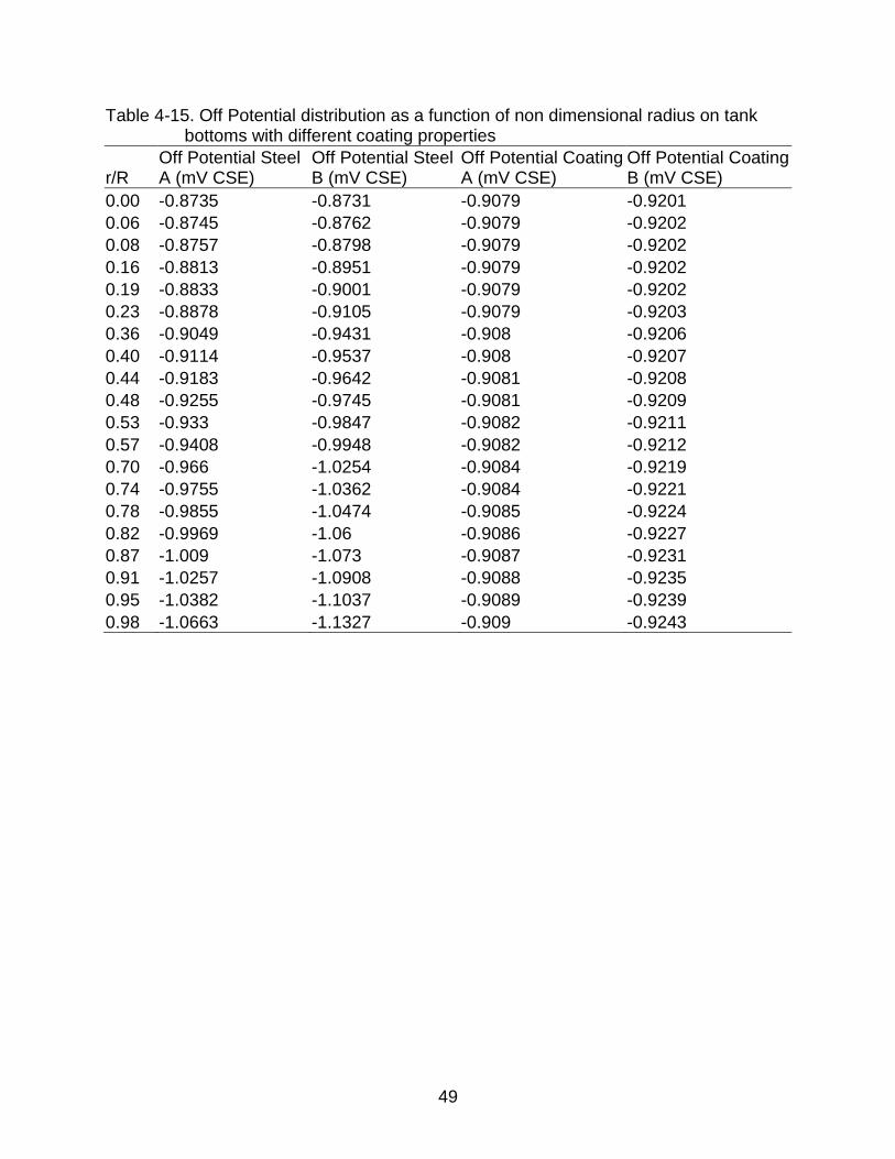
Table 4-15. Off Potential distribution as a function of non dimensional radius on tank bottoms with different coating properties
r/R Off Potential Steel A (mV CSE)
Off Potential Steel B (mV CSE)
Off Potential Coating A (mV CSE)
Off Potential Coating B (mV CSE)
0.00 -0.8735 -0.8731 -0.9079 -0.9201
0.06 -0.8745 -0.8762 -0.9079 -0.9202
0.08 -0.8757 -0.8798 -0.9079 -0.9202
0.16 -0.8813 -0.8951 -0.9079 -0.9202
0.19 -0.8833 -0.9001 -0.9079 -0.9202
0.23 -0.8878 -0.9105 -0.9079 -0.9203
0.36 -0.9049 -0.9431 -0.908 -0.9206
0.40 -0.9114 -0.9537 -0.908 -0.9207
0.44 -0.9183 -0.9642 -0.9081 -0.9208
0.48 -0.9255 -0.9745 -0.9081 -0.9209
0.53 -0.933 -0.9847 -0.9082 -0.9211
0.57 -0.9408 -0.9948 -0.9082 -0.9212
0.70 -0.966 -1.0254 -0.9084 -0.9219
0.74 -0.9755 -1.0362 -0.9084 -0.9221
0.78 -0.9855 -1.0474 -0.9085 -0.9224
0.82 -0.9969 -1.06 -0.9086 -0.9227
0.87 -1.009 -1.073 -0.9087 -0.9231
0.91 -1.0257 -1.0908 -0.9088 -0.9235
0.95 -1.0382 -1.1037 -0.9089 -0.9239
0.98 -1.0663 -1.1327 -0.909 -0.9243
50
Table 4-16. Model Parameters and simulation results for tank bottoms with different coating properties and holidays
Tank Coating Coating A with Steel B exposed
Coating B with Steel B exposed
Tank Diameter (m) 45.72 45.72
Number of element rings 12 12
Nodes in first ring 8 8
Length of Anode (m) 1 1
Diameter of Anode (m) 0.1 0.1
Depth of Anode (m) 1000 1000
Type of Anode ICCP - 160 ICCP - 16000
Potential Applied (V CSE) 160 16000
Output current of Anode (A) 3.184 36.98
Cross section area of tank bottom (m2) 1641.7 1641.7
Presence of Holiday on Tank Bottom Center Center
51
Table 4-17. Current and On Potential distribution as a function of Distance along the Radius on tank bottoms with different coating properties and holidays
Coating A, Steel B exposed
Coating B with Steel B exposed
Distance along the radius (m)
On Potential (V CSE)
Current Density (A/sq m)
On Potential (V CSE)
Current Density (A/sq m)
0 -1.07 -0.2034 -1.07 -0.2008
1.3188 -0.92 -0.114 -0.92 -0.1149
1.7585 -1.19 -9.90E-06 -1.19 -0.0002
3.6635 -17.46 -6.41E-04 -15.48 -0.0139
4.1397 -18.41 -6.78E-04 -16.23 -0.0146
5.0922 -19.84 -7.34E-04 -17.34 -0.0157
7.9497 -21.88 -8.14E-04 -19.02 -0.0174
8.9022 -22.28 -8.30E-04 -19.43 -0.0178
9.8547 -22.59 -8.42E-04 -19.82 -0.0182
10.8072 -22.86 -8.53E-04 -20.21 -0.0185
11.7597 -23.09 -8.62E-04 -20.61 -0.0189
12.7122 -23.29 -8.70E-04 -21.04 -0.0194
15.5697 -23.77 -8.89E-04 -22.57 -0.0209
16.5222 -23.91 -8.94E-04 -23.21 -0.0215
17.4747 -24.04 -8.99E-04 -23.93 -0.0222
18.4272 -24.16 -9.04E-04 -24.77 -0.023
19.3797 -24.29 -9.09E-04 -25.75 -0.024
20.3322 -24.41 -9.14E-04 -26.96 -0.0252
21.1504 -24.52 -9.18E-04 -28.22 -0.0264
21.8342 -24.62 -9.22E-04 -29.60 -0.0276
22.3471 -24.70 -9.25E-04 -30.87 -0.0282
52
Figure 4-1. Non Dimensional Ohmic resistance as a function of D with La, Da, Ha fixed
Figure 4-2. R/RDwight as a function of Distance of anode with La, Da, Ha fixed
Figure 4-3. Non Dimensional Ohmic resistance as a function of Da with La, Da, D fixed
53
Figure 4-4. R/RDwight as a function of Ha with La, Da, D fixed
Figure 4-5. Non Dimensional Ohmic resistance as a function of La with Da, Ha, D fixed
Figure 4-6. R/RDwight as a function of La with Da, Ha, D fixed
54
Figure 4-7. Non Dimensional Ohmic resistance as a function of Da with La, Ha, D fixed
Figure 4-8. R/RDwight as a function of Da with La, Ha, D fixed
Figure 4-9. Model of Single pipe
55
Figure 4-10. On Potential and Off Potential on Pipe #1 as a function of distance along the pipe for single pipe configuration
Figure 4-11. Current density on Pipe #1 as a function of distance along the pipe for single pipe configuration

56
Figure 4-12. Model of two Pipes with Single CP
Figure 4-13. On Potential and Off Potential on Pipe #1 as a function of distance along the pipe for two Pipes with Single CP configuration

57
Figure 4-14. Current Density on Pipe #1 as a function of distance along the pipe for two Pipes with Single CP configuration
Figure 4-15. On Potential and Off Potential on Pipe #2 as a function of distance along the pipe for two Pipes with Single CP configuration
58
Figure 4-16. On Potential and Off Potential on Pipe #2 as a function of distance along the pipe around the point of anode connection for two Pipes with one unprotected pipe configuration
Figure 4-17. Current Density on Pipe #2 as a function of distance along the pipe for two Pipes with one unprotected pipe configuration

59
Figure 4-18. Current Density on Pipe #2 as a function of distance along the pipe around the point of anode connection for two Pipes with one unprotected pipe configuration
Figure 4-19. Model of two pipes with independent Cp
60
Figure 4-20. On Potential and Off Potential on Pipe #1 as a function of distance along the pipe for two Pipes with independent CP configuration
Figure 4-21. Current density on Pipe #1 as a function of distance along the pipe for two Pipes with independent CP configuration
61
Figure 4-22. On Potential and Off Potential on Pipe #2 as a function of distance along the pipe for two Pipes with independent CP configuration
Figure 4-23. Current density on Pipe #2 as a function of distance along the pipe for two Pipes with independent CP configuration
62
Figure 4-24. Model of 2 pipes with Independent CP and coating flaw on one pipe configuration
Figure 4-25. On Potential and Off Potential on Pipe #1 as a function of distance along the pipe for two pipes with Independent CP and coating flaw on one pipe configuration
63
Figure 4-26. Current density on Pipe #1 as a function of distance along the pipe for two pipes with Independent CP and coating flaw on one pipe configuration
Figure 4-27. On Potential and Off Potential on Pipe #2 as a function of distance along the pipe for two pipes with Independent CP and coating flaw on one pipe configuration
64
Figure 4-28. Current density on Pipe #2 as a function of distance along the pipe for two pipes with Independent CP and coating flaw on one pipe configuration
Figure 4-29. Steel A
65
Figure 4-30. Steel B
Figure 4-31. Coating A
66
Figure 4-32. Coating B
Figure 4-33. Non dimensional Current Density as a function of non dimensional radius on Tank Bottoms with different coating properties
67
Figure 4-34. Off Potential as a function of non dimensional radius on Tank Bottoms with
different coating properties
Figure 4-35. Coating A with holiday exposing Steel B
68
Figure 4-36. Coating B with holiday exposing Steel B
Figure 4-37. Current Density as a function of Distance along the Radius on Tank
Bottoms with different coating properties and holidays
69
Figure 4-38. On Potential as a function of Distance along the Radius on Tank Bottoms with different coating properties and holidays
70
CHAPTER 5 CONCLUSIONS
The performance of the cathodic protection was analyzed using the dimensional
analysis of the parameters associated with the anode. Several cases were studied to
understand the interaction between two cathodic protection system installations in
pipelines modeled in cross over configuration. The recent tank bottom studies were
extended to understand the effect of protection current on coated tank bottoms and
when coating flaws are present in the tank bottoms.
The dimensional analysis of the anode parameters showed that the length,
diameter and depth of the anode are the dominant parameters which affect the
performance of cathodic protection system.
Cathodic interference effects in pipelines were observed in cases where the two
pipes placed in a cross over configuration with one pipe connected to a cathodic
protection anode, both pipes having independent cathodic protection installations, and
both pipes having independent cathodic protection installations with a coating flaw
present on one pipe. The potential and current distribution on one pipe was affected by
the presence of CP on the other pipe. When the pipes in cross-over configuration have
independent CP and a holiday was present on pipe #1, the potential distribution
indicated that the metal exposed by the coating defect was anodic and was subject to
corrosion. On pipe #2, a similar anodic region was observed, despite the absence of a
holiday. This is an indication of the interaction between the CP systems on both the
pipes.
The tank bottoms with no coatings present can be protected by using a deep well
ground bed placed far from the tank bottom without over protecting any region of the

71
tank bottom. The only concern is that the applied potential be sufficient to drive the
necessary current. A non-uniform potential distribution was observed along the radius of
the tank bottom. The current density was highest at the outer ring of the tank bottom
and least at the center. The off potential was more cathodic at the outer ring than the
center of the tank bottom.
The coated tank bottoms had a uniform current distribution along the radius of the
tank. The magnitude of the protection current required was significantly smaller than the
case when the tank bottom had no coating. The protection current required for tank
bottom with Coating A was lower than with Coating B as the resistivity and oxygen
blocking property of Coating A was higher. The maximum radius protected was larger in
the case of tank bottom with Coating A than Coating B.
The distribution of protection current was non uniform when coating flaws were
present at the center of the tank in coated tank bottoms. Most of the protection current
was directed towards the site of coating flaw. The protection current required in the case
where tank bottom had Coating A and Steel B exposed in holiday was less than the
case of tank bottom with Coating B with Steel B exposed as the resistivity and oxygen
blocking property of Coating A is higher. When a large driving force was applied to
ensure minimum protection of the center of tank bottom where coating flaw was
present, the other regions of the tank bottom were overprotected.
72
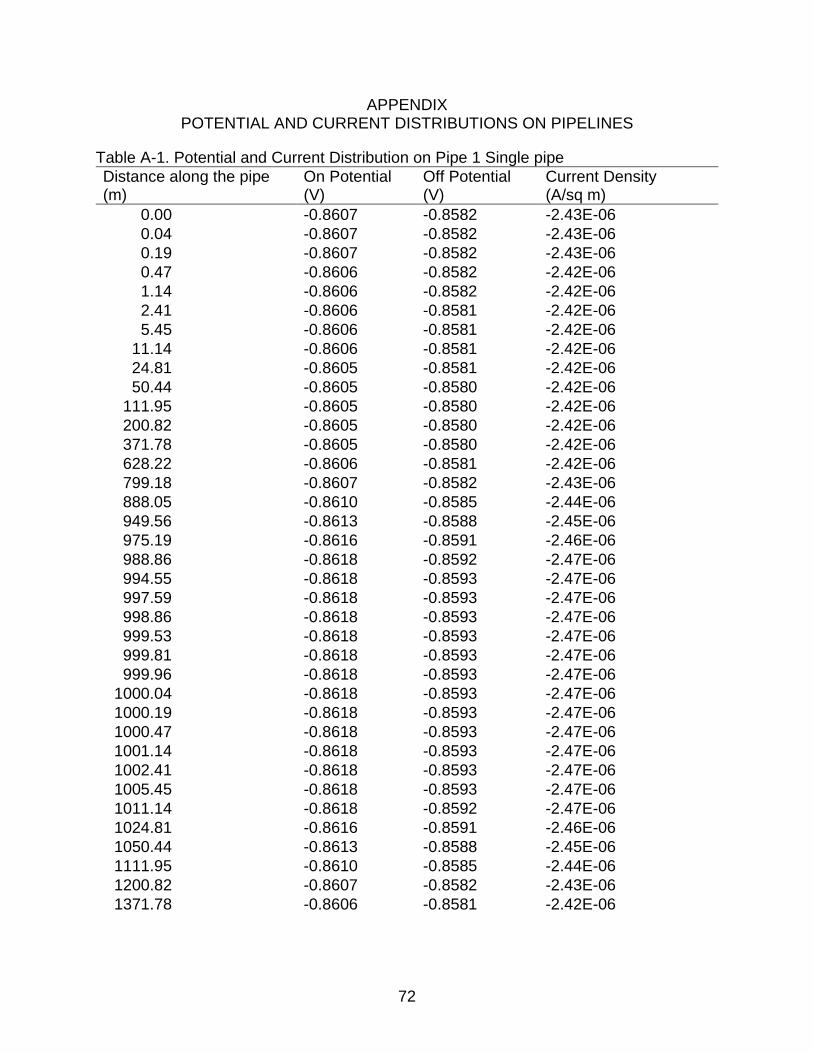
APPENDIX POTENTIAL AND CURRENT DISTRIBUTIONS ON PIPELINES
Table A-1. Potential and Current Distribution on Pipe 1 Single pipe
Distance along the pipe (m)
On Potential (V)
Off Potential (V)
Current Density (A/sq m)
0.00 -0.8607 -0.8582 -2.43E-06
0.04 -0.8607 -0.8582 -2.43E-06
0.19 -0.8607 -0.8582 -2.43E-06
0.47 -0.8606 -0.8582 -2.42E-06
1.14 -0.8606 -0.8582 -2.42E-06
2.41 -0.8606 -0.8581 -2.42E-06
5.45 -0.8606 -0.8581 -2.42E-06
11.14 -0.8606 -0.8581 -2.42E-06
24.81 -0.8605 -0.8581 -2.42E-06
50.44 -0.8605 -0.8580 -2.42E-06
111.95 -0.8605 -0.8580 -2.42E-06
200.82 -0.8605 -0.8580 -2.42E-06
371.78 -0.8605 -0.8580 -2.42E-06
628.22 -0.8606 -0.8581 -2.42E-06
799.18 -0.8607 -0.8582 -2.43E-06
888.05 -0.8610 -0.8585 -2.44E-06
949.56 -0.8613 -0.8588 -2.45E-06
975.19 -0.8616 -0.8591 -2.46E-06
988.86 -0.8618 -0.8592 -2.47E-06
994.55 -0.8618 -0.8593 -2.47E-06
997.59 -0.8618 -0.8593 -2.47E-06
998.86 -0.8618 -0.8593 -2.47E-06
999.53 -0.8618 -0.8593 -2.47E-06
999.81 -0.8618 -0.8593 -2.47E-06
999.96 -0.8618 -0.8593 -2.47E-06
1000.04 -0.8618 -0.8593 -2.47E-06
1000.19 -0.8618 -0.8593 -2.47E-06
1000.47 -0.8618 -0.8593 -2.47E-06
1001.14 -0.8618 -0.8593 -2.47E-06
1002.41 -0.8618 -0.8593 -2.47E-06
1005.45 -0.8618 -0.8593 -2.47E-06
1011.14 -0.8618 -0.8592 -2.47E-06
1024.81 -0.8616 -0.8591 -2.46E-06
1050.44 -0.8613 -0.8588 -2.45E-06
1111.95 -0.8610 -0.8585 -2.44E-06
1200.82 -0.8607 -0.8582 -2.43E-06
1371.78 -0.8606 -0.8581 -2.42E-06

73
Table. A-1. Continued
Distance along the pipe (m)
On Potential (V)
Off Potential (V)
Current Density (A/sq m)
1888.05 -0.8605 -0.8580 -2.42E-06
1949.56 -0.8605 -0.8580 -2.42E-06
1975.19 -0.8605 -0.8581 -2.42E-06
1988.86 -0.8606 -0.8581 -2.42E-06
1994.55 -0.8606 -0.8581 -2.42E-06
1997.59 -0.8606 -0.8581 -2.42E-06
1998.86 -0.8606 -0.8582 -2.42E-06
1999.53 -0.8606 -0.8582 -2.42E-06
1999.81 -0.8607 -0.8582 -2.43E-06
1999.96 -0.8607 -0.8582 -2.43E-06
2000.00 -0.8607 -0.8582 -2.43E-06
74
Table A-2. Potential and Current Distributions on Pipe1 and Pipe2
Pipe 1 Pipe 2 Distance along the pipe (m)
On Potential (V)
Off Potential (V)
Current Density (A/sq m)
On Potential (V)
Off Potential (V)
Current Density (A/sq m)
0.00 -0.8607 -0.8582 -2.43E-06 -0.6355 -0.6355 8.59E-10
0.04 -0.8607 -0.8582 -2.43E-06 -0.6355 -0.6355 8.59E-10
0.19 -0.8607 -0.8582 -2.43E-06 -0.6355 -0.6355 8.59E-10
0.47 -0.8606 -0.8582 -2.42E-06 -0.6355 -0.6355 8.58E-10
1.14 -0.8606 -0.8582 -2.42E-06 -0.6355 -0.6355 8.58E-10
2.41 -0.8606 -0.8581 -2.42E-06 -0.6355 -0.6355 8.58E-10
5.45 -0.8606 -0.8581 -2.42E-06 -0.6355 -0.6355 8.58E-10
11.14 -0.8606 -0.8581 -2.42E-06 -0.6355 -0.6355 8.57E-10
24.81 -0.8605 -0.8581 -2.42E-06 -0.6355 -0.6355 8.56E-10
50.44 -0.8605 -0.8580 -2.42E-06 -0.6355 -0.6355 8.53E-10
111.95 -0.8605 -0.8580 -2.42E-06 -0.6355 -0.6355 8.45E-10
200.82 -0.8605 -0.8580 -2.42E-06 -0.6355 -0.6355 8.37E-10
371.78 -0.8605 -0.8580 -2.42E-06 -0.6355 -0.6355 7.77E-10
628.22 -0.8605 -0.8581 -2.42E-06 -0.6356 -0.6356 5.83E-10
799.18 -0.8606 -0.8582 -2.42E-06 -0.6356 -0.6356 1.75E-10
888.05 -0.8608 -0.8583 -2.43E-06 -0.6357 -0.6357 -5.50E-10
949.56 -0.8610 -0.8585 -2.44E-06 -0.6359 -0.6359 -1.46E-09
975.19 -0.8611 -0.8587 -2.44E-06 -0.6360 -0.6360 -2.21E-09
988.86 -0.8613 -0.8588 -2.45E-06 -0.6361 -0.6360 -2.55E-09
994.55 -0.8613 -0.8588 -2.45E-06 -0.6361 -0.6361 -2.56E-09
997.59 -0.8613 -0.8588 -2.45E-06 -0.6360 -0.6360 -2.47E-09
998.86 -0.8614 -0.8589 -2.45E-06 -0.6360 -0.6360 -2.34E-09
999.53 -0.8614 -0.8589 -2.45E-06 -0.6360 -0.6360 -2.25E-09
999.81 -0.8614 -0.8589 -2.45E-06 -0.6360 -0.6360 -2.22E-09
999.96 -0.8614 -0.8589 -2.45E-06 -0.6360 -0.6360 -2.22E-09
1000.04 -0.8614 -0.8589 -2.45E-06 -0.6360 -0.6360 -2.22E-09
1000.19 -0.8614 -0.8589 -2.45E-06 -0.6360 -0.6360 -2.25E-09
1000.47 -0.8614 -0.8589 -2.45E-06 -0.6360 -0.6360 -2.31E-09
1001.14 -0.8614 -0.8589 -2.45E-06 -0.6360 -0.6360 -2.49E-09
1002.41 -0.8614 -0.8589 -2.45E-06 -0.6361 -0.6361 -2.78E-09
1005.45 -0.8614 -0.8589 -2.46E-06 -0.6362 -0.6362 -3.27E-09
1009.88 -0.8615 -0.8590 -2.46E-06 -0.6363 -0.6363 -3.85E-09
1018.52 -0.8616 -0.8591 -2.46E-06 -0.6364 -0.6364 -4.70E-09
1031.48 -0.8617 -0.8592 -2.47E-06 -0.6366 -0.6366 -5.76E-09
1040.12 -0.8618 -0.8593 -2.47E-06 -0.6366 -0.6366 -6.30E-09
1044.55 -0.8618 -0.8593 -2.47E-06 -0.6367 -0.6367 -6.44E-09
1047.59 -0.8618 -0.8593 -2.47E-06 -0.6367 -0.6367 -6.52E-09
1048.86 -0.8618 -0.8593 -2.47E-06 -0.6367 -0.6367 -6.54E-09
1049.53 -0.8618 -0.8593 -2.47E-06 -0.6367 -0.6367 -6.54E-09
1049.81 -0.8618 -0.8593 -2.47E-06 -0.6367 -0.6367 -6.55E-09

75
Table A-2. Continued
Pipe 1 Pipe 2 Distance along the pipe (m)
On Potential (V)
Off Potential (V)
Current Density (A/sq m)
On Potential (V)
Off Potential (V)
Current Density (A/sq m)
1049.96 -0.8618 -0.8593 -2.47E-06 -0.6367 -0.6367 -6.55E-09
1050.04 -0.8618 -0.8593 -2.47E-06 -0.6367 -0.6367 -6.55E-09
1050.19 -0.8618 -0.8593 -2.47E-06 -0.6367 -0.6367 -6.55E-09
1050.47 -0.8618 -0.8593 -2.47E-06 -0.6367 -0.6367 -6.55E-09
1051.14 -0.8618 -0.8593 -2.47E-06 -0.6367 -0.6367 -6.56E-09
1052.41 -0.8618 -0.8593 -2.47E-06 -0.6367 -0.6367 -6.56E-09
1055.45 -0.8618 -0.8593 -2.47E-06 -0.6367 -0.6367 -6.54E-09
1061.14 -0.8618 -0.8592 -2.47E-06 -0.6367 -0.6367 -6.46E-09
1074.81 -0.8616 -0.8591 -2.46E-06 -0.6366 -0.6366 -5.78E-09
1100.44 -0.8613 -0.8588 -2.45E-06 -0.6363 -0.6363 -4.00E-09
1161.95 -0.8610 -0.8585 -2.44E-06 -0.6359 -0.6359 -1.85E-09
1247.70 -0.8607 -0.8582 -2.43E-06 -0.6357 -0.6357 -3.65E-10
1406.16 -0.8606 -0.8581 -2.42E-06 -0.6356 -0.6356 3.44E-10
1643.84 -0.8605 -0.8580 -2.42E-06 -0.6355 -0.6356 6.66E-10
1802.30 -0.8605 -0.8580 -2.42E-06 -0.6355 -0.6355 7.68E-10
1888.05 -0.8605 -0.8580 -2.42E-06 -0.6355 -0.6355 7.86E-10
1949.56 -0.8605 -0.8581 -2.42E-06 -0.6355 -0.6355 8.02E-10
1975.19 -0.8605 -0.8581 -2.42E-06 -0.6355 -0.6355 8.07E-10
1988.86 -0.8606 -0.8581 -2.42E-06 -0.6355 -0.6355 8.10E-10
1994.55 -0.8606 -0.8581 -2.42E-06 -0.6355 -0.6355 8.11E-10
1997.59 -0.8606 -0.8581 -2.42E-06 -0.6355 -0.6355 8.12E-10
1998.86 -0.8606 -0.8582 -2.42E-06 -0.6355 -0.6355 8.12E-10
1999.53 -0.8606 -0.8582 -2.43E-06 -0.6355 -0.6355 8.12E-10
1999.81 -0.8607 -0.8582 -2.43E-06 -0.6355 -0.6355 8.12E-10
1999.96 -0.8607 -0.8582 -2.43E-06 -0.6355 -0.6355 8.12E-10
2000.00 -0.8607 -0.8582 -2.43E-06 -0.6355 -0.6355 8.12E-10
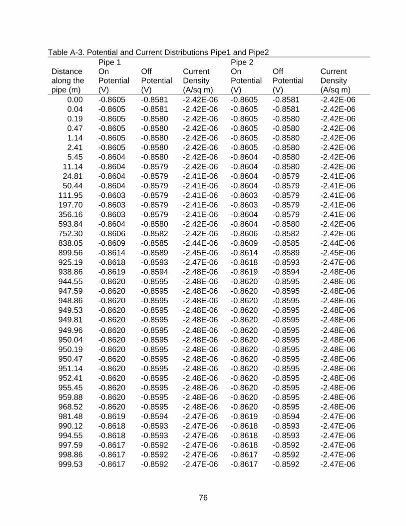
76
Table A-3. Potential and Current Distributions Pipe1 and Pipe2
Pipe 1 Pipe 2 Distance along the pipe (m)
On Potential (V)
Off Potential (V)
Current Density (A/sq m)
On Potential (V)
Off Potential (V)
Current Density (A/sq m)
0.00 -0.8605 -0.8581 -2.42E-06 -0.8605 -0.8581 -2.42E-06
0.04 -0.8605 -0.8581 -2.42E-06 -0.8605 -0.8581 -2.42E-06
0.19 -0.8605 -0.8580 -2.42E-06 -0.8605 -0.8580 -2.42E-06
0.47 -0.8605 -0.8580 -2.42E-06 -0.8605 -0.8580 -2.42E-06
1.14 -0.8605 -0.8580 -2.42E-06 -0.8605 -0.8580 -2.42E-06
2.41 -0.8605 -0.8580 -2.42E-06 -0.8605 -0.8580 -2.42E-06
5.45 -0.8604 -0.8580 -2.42E-06 -0.8604 -0.8580 -2.42E-06
11.14 -0.8604 -0.8579 -2.42E-06 -0.8604 -0.8580 -2.42E-06
24.81 -0.8604 -0.8579 -2.41E-06 -0.8604 -0.8579 -2.41E-06
50.44 -0.8604 -0.8579 -2.41E-06 -0.8604 -0.8579 -2.41E-06
111.95 -0.8603 -0.8579 -2.41E-06 -0.8603 -0.8579 -2.41E-06
197.70 -0.8603 -0.8579 -2.41E-06 -0.8603 -0.8579 -2.41E-06
356.16 -0.8603 -0.8579 -2.41E-06 -0.8604 -0.8579 -2.41E-06
593.84 -0.8604 -0.8580 -2.42E-06 -0.8604 -0.8580 -2.42E-06
752.30 -0.8606 -0.8582 -2.42E-06 -0.8606 -0.8582 -2.42E-06
838.05 -0.8609 -0.8585 -2.44E-06 -0.8609 -0.8585 -2.44E-06
899.56 -0.8614 -0.8589 -2.45E-06 -0.8614 -0.8589 -2.45E-06
925.19 -0.8618 -0.8593 -2.47E-06 -0.8618 -0.8593 -2.47E-06
938.86 -0.8619 -0.8594 -2.48E-06 -0.8619 -0.8594 -2.48E-06
944.55 -0.8620 -0.8595 -2.48E-06 -0.8620 -0.8595 -2.48E-06
947.59 -0.8620 -0.8595 -2.48E-06 -0.8620 -0.8595 -2.48E-06
948.86 -0.8620 -0.8595 -2.48E-06 -0.8620 -0.8595 -2.48E-06
949.53 -0.8620 -0.8595 -2.48E-06 -0.8620 -0.8595 -2.48E-06
949.81 -0.8620 -0.8595 -2.48E-06 -0.8620 -0.8595 -2.48E-06
949.96 -0.8620 -0.8595 -2.48E-06 -0.8620 -0.8595 -2.48E-06
950.04 -0.8620 -0.8595 -2.48E-06 -0.8620 -0.8595 -2.48E-06
950.19 -0.8620 -0.8595 -2.48E-06 -0.8620 -0.8595 -2.48E-06
950.47 -0.8620 -0.8595 -2.48E-06 -0.8620 -0.8595 -2.48E-06
951.14 -0.8620 -0.8595 -2.48E-06 -0.8620 -0.8595 -2.48E-06
952.41 -0.8620 -0.8595 -2.48E-06 -0.8620 -0.8595 -2.48E-06
955.45 -0.8620 -0.8595 -2.48E-06 -0.8620 -0.8595 -2.48E-06
959.88 -0.8620 -0.8595 -2.48E-06 -0.8620 -0.8595 -2.48E-06
968.52 -0.8620 -0.8595 -2.48E-06 -0.8620 -0.8595 -2.48E-06
981.48 -0.8619 -0.8594 -2.47E-06 -0.8619 -0.8594 -2.47E-06
990.12 -0.8618 -0.8593 -2.47E-06 -0.8618 -0.8593 -2.47E-06
994.55 -0.8618 -0.8593 -2.47E-06 -0.8618 -0.8593 -2.47E-06
997.59 -0.8617 -0.8592 -2.47E-06 -0.8618 -0.8592 -2.47E-06
998.86 -0.8617 -0.8592 -2.47E-06 -0.8617 -0.8592 -2.47E-06
999.53 -0.8617 -0.8592 -2.47E-06 -0.8617 -0.8592 -2.47E-06
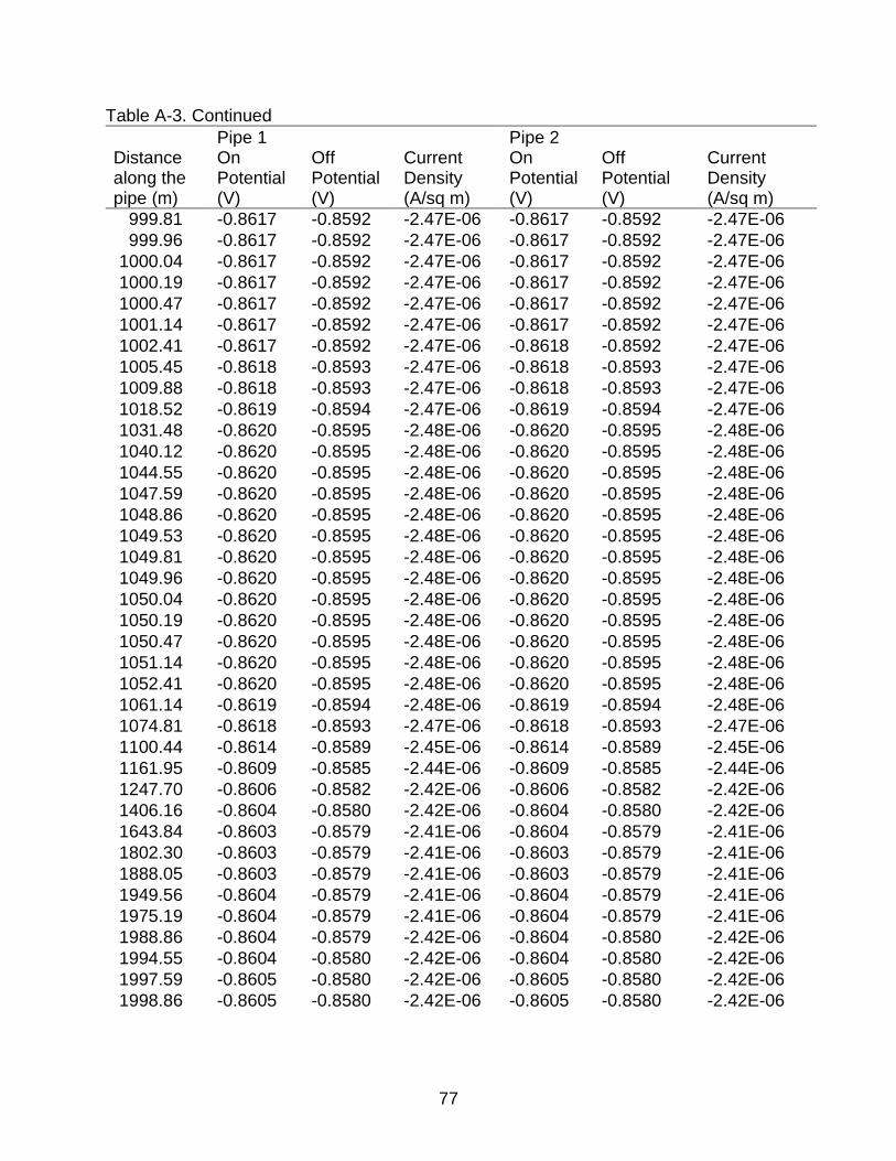
77
Table A-3. Continued
Pipe 1 Pipe 2 Distance along the pipe (m)
On Potential (V)
Off Potential (V)
Current Density (A/sq m)
On Potential (V)
Off Potential (V)
Current Density (A/sq m)
999.81 -0.8617 -0.8592 -2.47E-06 -0.8617 -0.8592 -2.47E-06
999.96 -0.8617 -0.8592 -2.47E-06 -0.8617 -0.8592 -2.47E-06
1000.04 -0.8617 -0.8592 -2.47E-06 -0.8617 -0.8592 -2.47E-06
1000.19 -0.8617 -0.8592 -2.47E-06 -0.8617 -0.8592 -2.47E-06
1000.47 -0.8617 -0.8592 -2.47E-06 -0.8617 -0.8592 -2.47E-06
1001.14 -0.8617 -0.8592 -2.47E-06 -0.8617 -0.8592 -2.47E-06
1002.41 -0.8617 -0.8592 -2.47E-06 -0.8618 -0.8592 -2.47E-06
1005.45 -0.8618 -0.8593 -2.47E-06 -0.8618 -0.8593 -2.47E-06
1009.88 -0.8618 -0.8593 -2.47E-06 -0.8618 -0.8593 -2.47E-06
1018.52 -0.8619 -0.8594 -2.47E-06 -0.8619 -0.8594 -2.47E-06
1031.48 -0.8620 -0.8595 -2.48E-06 -0.8620 -0.8595 -2.48E-06
1040.12 -0.8620 -0.8595 -2.48E-06 -0.8620 -0.8595 -2.48E-06
1044.55 -0.8620 -0.8595 -2.48E-06 -0.8620 -0.8595 -2.48E-06
1047.59 -0.8620 -0.8595 -2.48E-06 -0.8620 -0.8595 -2.48E-06
1048.86 -0.8620 -0.8595 -2.48E-06 -0.8620 -0.8595 -2.48E-06
1049.53 -0.8620 -0.8595 -2.48E-06 -0.8620 -0.8595 -2.48E-06
1049.81 -0.8620 -0.8595 -2.48E-06 -0.8620 -0.8595 -2.48E-06
1049.96 -0.8620 -0.8595 -2.48E-06 -0.8620 -0.8595 -2.48E-06
1050.04 -0.8620 -0.8595 -2.48E-06 -0.8620 -0.8595 -2.48E-06
1050.19 -0.8620 -0.8595 -2.48E-06 -0.8620 -0.8595 -2.48E-06
1050.47 -0.8620 -0.8595 -2.48E-06 -0.8620 -0.8595 -2.48E-06
1051.14 -0.8620 -0.8595 -2.48E-06 -0.8620 -0.8595 -2.48E-06
1052.41 -0.8620 -0.8595 -2.48E-06 -0.8620 -0.8595 -2.48E-06
1061.14 -0.8619 -0.8594 -2.48E-06 -0.8619 -0.8594 -2.48E-06
1074.81 -0.8618 -0.8593 -2.47E-06 -0.8618 -0.8593 -2.47E-06
1100.44 -0.8614 -0.8589 -2.45E-06 -0.8614 -0.8589 -2.45E-06
1161.95 -0.8609 -0.8585 -2.44E-06 -0.8609 -0.8585 -2.44E-06
1247.70 -0.8606 -0.8582 -2.42E-06 -0.8606 -0.8582 -2.42E-06
1406.16 -0.8604 -0.8580 -2.42E-06 -0.8604 -0.8580 -2.42E-06
1643.84 -0.8603 -0.8579 -2.41E-06 -0.8604 -0.8579 -2.41E-06
1802.30 -0.8603 -0.8579 -2.41E-06 -0.8603 -0.8579 -2.41E-06
1888.05 -0.8603 -0.8579 -2.41E-06 -0.8603 -0.8579 -2.41E-06
1949.56 -0.8604 -0.8579 -2.41E-06 -0.8604 -0.8579 -2.41E-06
1975.19 -0.8604 -0.8579 -2.41E-06 -0.8604 -0.8579 -2.41E-06
1988.86 -0.8604 -0.8579 -2.42E-06 -0.8604 -0.8580 -2.42E-06
1994.55 -0.8604 -0.8580 -2.42E-06 -0.8604 -0.8580 -2.42E-06
1997.59 -0.8605 -0.8580 -2.42E-06 -0.8605 -0.8580 -2.42E-06
1998.86 -0.8605 -0.8580 -2.42E-06 -0.8605 -0.8580 -2.42E-06
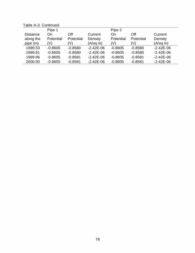
78
Table A-3. Continued
Pipe 1 Pipe 2 Distance along the pipe (m)
On Potential (V)
Off Potential (V)
Current Density (A/sq m)
On Potential (V)
Off Potential (V)
Current Density (A/sq m)
1999.53 -0.8605 -0.8580 -2.42E-06 -0.8605 -0.8580 -2.42E-06
1999.81 -0.8605 -0.8580 -2.42E-06 -0.8605 -0.8580 -2.42E-06
1999.96 -0.8605 -0.8581 -2.42E-06 -0.8605 -0.8581 -2.42E-06
2000.00 -0.8605 -0.8581 -2.42E-06 -0.8605 -0.8581 -2.42E-06
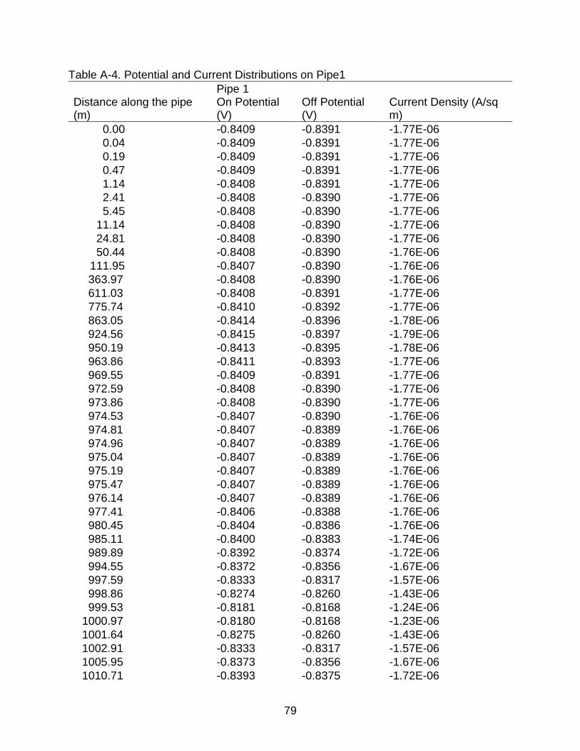
79
Table A-4. Potential and Current Distributions on Pipe1
Pipe 1 Distance along the pipe (m)
On Potential (V)
Off Potential (V)
Current Density (A/sq m)
0.00 -0.8409 -0.8391 -1.77E-06
0.04 -0.8409 -0.8391 -1.77E-06
0.19 -0.8409 -0.8391 -1.77E-06
0.47 -0.8409 -0.8391 -1.77E-06
1.14 -0.8408 -0.8391 -1.77E-06
2.41 -0.8408 -0.8390 -1.77E-06
5.45 -0.8408 -0.8390 -1.77E-06
11.14 -0.8408 -0.8390 -1.77E-06
24.81 -0.8408 -0.8390 -1.77E-06
50.44 -0.8408 -0.8390 -1.76E-06
111.95 -0.8407 -0.8390 -1.76E-06
363.97 -0.8408 -0.8390 -1.76E-06
611.03 -0.8408 -0.8391 -1.77E-06
775.74 -0.8410 -0.8392 -1.77E-06
863.05 -0.8414 -0.8396 -1.78E-06
924.56 -0.8415 -0.8397 -1.79E-06
950.19 -0.8413 -0.8395 -1.78E-06
963.86 -0.8411 -0.8393 -1.77E-06
969.55 -0.8409 -0.8391 -1.77E-06
972.59 -0.8408 -0.8390 -1.77E-06
973.86 -0.8408 -0.8390 -1.77E-06
974.53 -0.8407 -0.8390 -1.76E-06
974.81 -0.8407 -0.8389 -1.76E-06
974.96 -0.8407 -0.8389 -1.76E-06
975.04 -0.8407 -0.8389 -1.76E-06
975.19 -0.8407 -0.8389 -1.76E-06
975.47 -0.8407 -0.8389 -1.76E-06
976.14 -0.8407 -0.8389 -1.76E-06
977.41 -0.8406 -0.8388 -1.76E-06
980.45 -0.8404 -0.8386 -1.76E-06
985.11 -0.8400 -0.8383 -1.74E-06
989.89 -0.8392 -0.8374 -1.72E-06
994.55 -0.8372 -0.8356 -1.67E-06
997.59 -0.8333 -0.8317 -1.57E-06
998.86 -0.8274 -0.8260 -1.43E-06
999.53 -0.8181 -0.8168 -1.24E-06
1000.97 -0.8180 -0.8168 -1.23E-06
1001.64 -0.8275 -0.8260 -1.43E-06
1002.91 -0.8333 -0.8317 -1.57E-06
1005.95 -0.8373 -0.8356 -1.67E-06
1010.71 -0.8393 -0.8375 -1.72E-06
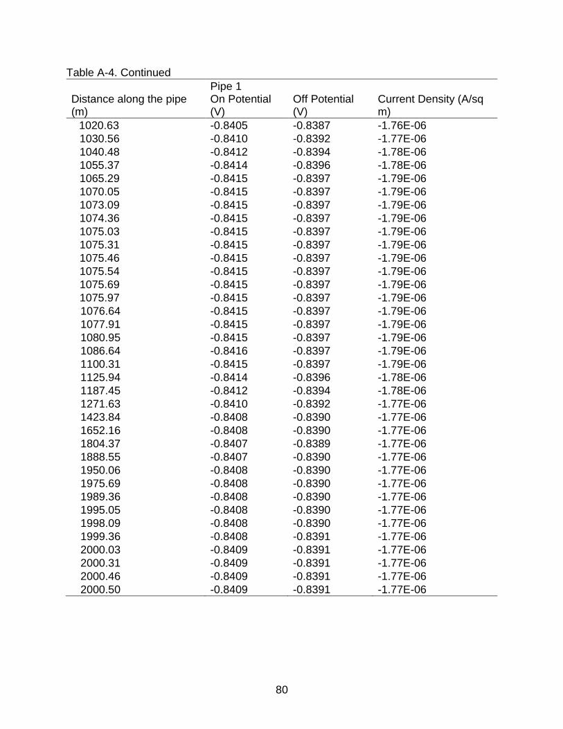
80
Table A-4. Continued
Pipe 1 Distance along the pipe (m)
On Potential (V)
Off Potential (V)
Current Density (A/sq m)
1020.63 -0.8405 -0.8387 -1.76E-06
1030.56 -0.8410 -0.8392 -1.77E-06
1040.48 -0.8412 -0.8394 -1.78E-06
1055.37 -0.8414 -0.8396 -1.78E-06
1065.29 -0.8415 -0.8397 -1.79E-06
1070.05 -0.8415 -0.8397 -1.79E-06
1073.09 -0.8415 -0.8397 -1.79E-06
1074.36 -0.8415 -0.8397 -1.79E-06
1075.03 -0.8415 -0.8397 -1.79E-06
1075.31 -0.8415 -0.8397 -1.79E-06
1075.46 -0.8415 -0.8397 -1.79E-06
1075.54 -0.8415 -0.8397 -1.79E-06
1075.69 -0.8415 -0.8397 -1.79E-06
1075.97 -0.8415 -0.8397 -1.79E-06
1076.64 -0.8415 -0.8397 -1.79E-06
1077.91 -0.8415 -0.8397 -1.79E-06
1080.95 -0.8415 -0.8397 -1.79E-06
1086.64 -0.8416 -0.8397 -1.79E-06
1100.31 -0.8415 -0.8397 -1.79E-06
1125.94 -0.8414 -0.8396 -1.78E-06
1187.45 -0.8412 -0.8394 -1.78E-06
1271.63 -0.8410 -0.8392 -1.77E-06
1423.84 -0.8408 -0.8390 -1.77E-06
1652.16 -0.8408 -0.8390 -1.77E-06
1804.37 -0.8407 -0.8389 -1.77E-06
1888.55 -0.8407 -0.8390 -1.77E-06
1950.06 -0.8408 -0.8390 -1.77E-06
1975.69 -0.8408 -0.8390 -1.77E-06
1989.36 -0.8408 -0.8390 -1.77E-06
1995.05 -0.8408 -0.8390 -1.77E-06
1998.09 -0.8408 -0.8390 -1.77E-06
1999.36 -0.8408 -0.8391 -1.77E-06
2000.03 -0.8409 -0.8391 -1.77E-06
2000.31 -0.8409 -0.8391 -1.77E-06
2000.46 -0.8409 -0.8391 -1.77E-06
2000.50 -0.8409 -0.8391 -1.77E-06

81
Table A-5. Potential and Current Distribution on Pipe2
Pipe 2 Distance along the pipe (m)
On Potential (V)
Off Potential (V)
Current Density (A/sq m)
0.00 -0.8607 -0.8582 -2.43E-06
0.04 -0.8607 -0.8582 -2.43E-06
0.19 -0.8607 -0.8582 -2.43E-06
0.47 -0.8607 -0.8582 -2.43E-06
1.14 -0.8607 -0.8582 -2.43E-06
2.41 -0.8606 -0.8582 -2.42E-06
5.45 -0.8606 -0.8581 -2.42E-06
11.14 -0.8606 -0.8581 -2.42E-06
24.81 -0.8606 -0.8581 -2.42E-06
50.44 -0.8605 -0.8581 -2.42E-06
111.95 -0.8605 -0.8581 -2.42E-06
196.13 -0.8605 -0.8580 -2.42E-06
348.34 -0.8605 -0.8581 -2.42E-06
576.66 -0.8606 -0.8581 -2.42E-06
728.87 -0.8607 -0.8583 -2.43E-06
813.05 -0.8609 -0.8585 -2.44E-06
874.56 -0.8612 -0.8587 -2.45E-06
913.86 -0.8613 -0.8588 -2.45E-06
919.55 -0.8613 -0.8588 -2.45E-06
922.59 -0.8613 -0.8588 -2.45E-06
923.86 -0.8613 -0.8588 -2.45E-06
924.53 -0.8613 -0.8588 -2.45E-06
924.81 -0.8613 -0.8588 -2.45E-06
924.96 -0.8613 -0.8588 -2.45E-06
925.04 -0.8613 -0.8588 -2.45E-06
925.19 -0.8613 -0.8588 -2.45E-06
925.47 -0.8613 -0.8588 -2.45E-06
926.14 -0.8613 -0.8588 -2.45E-06
927.41 -0.8613 -0.8588 -2.45E-06
930.45 -0.8613 -0.8588 -2.45E-06
935.21 -0.8612 -0.8588 -2.45E-06
945.13 -0.8612 -0.8587 -2.45E-06
955.06 -0.8611 -0.8586 -2.44E-06
964.98 -0.8608 -0.8584 -2.43E-06
979.87 -0.8603 -0.8578 -2.41E-06
989.79 -0.8591 -0.8567 -2.37E-06
994.55 -0.8570 -0.8547 -2.29E-06
997.59 -0.8531 -0.8510 -2.15E-06
998.86 -0.8475 -0.8455 -1.97E-06
999.53 -0.8424 -0.8406 -1.81E-06
999.81 -0.8396 -0.8378 -1.73E-06
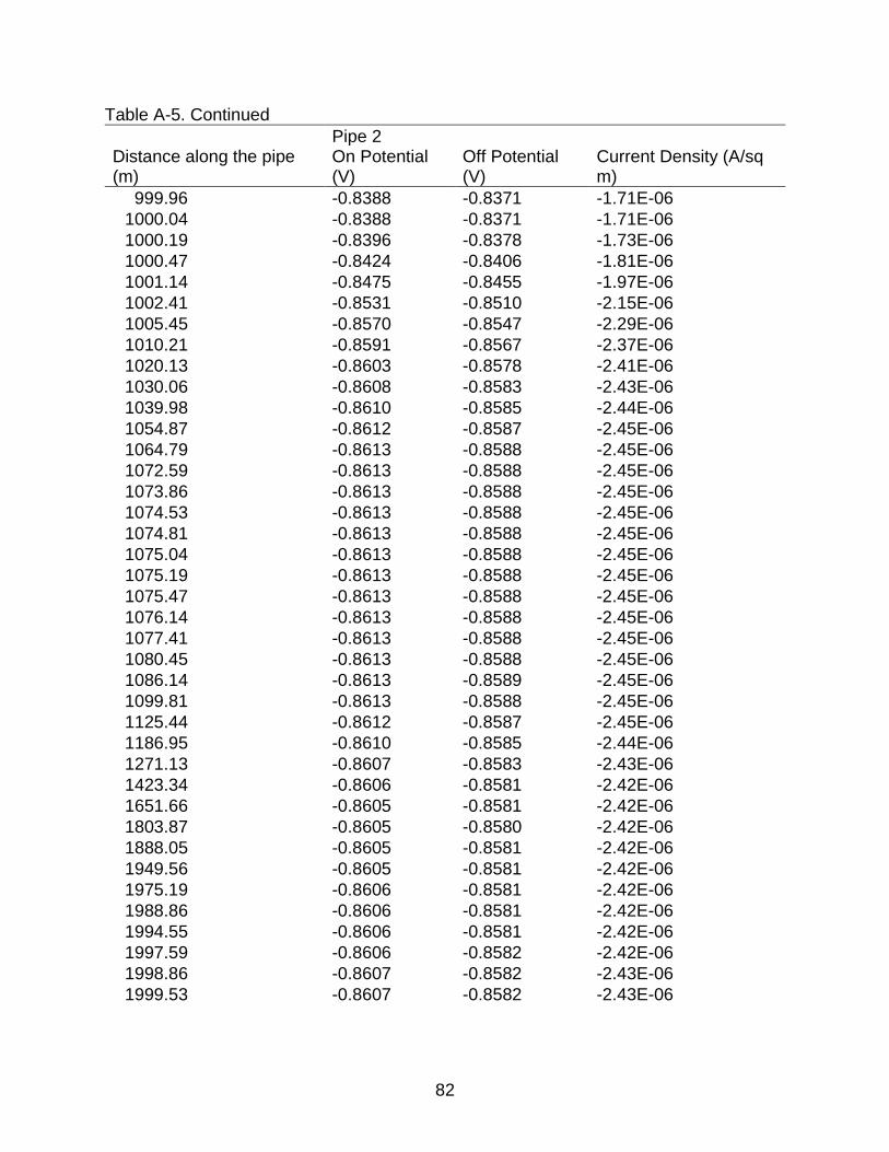
82
Table A-5. Continued
Pipe 2 Distance along the pipe (m)
On Potential (V)
Off Potential (V)
Current Density (A/sq m)
999.96 -0.8388 -0.8371 -1.71E-06
1000.04 -0.8388 -0.8371 -1.71E-06
1000.19 -0.8396 -0.8378 -1.73E-06
1000.47 -0.8424 -0.8406 -1.81E-06
1001.14 -0.8475 -0.8455 -1.97E-06
1002.41 -0.8531 -0.8510 -2.15E-06
1005.45 -0.8570 -0.8547 -2.29E-06
1010.21 -0.8591 -0.8567 -2.37E-06
1020.13 -0.8603 -0.8578 -2.41E-06
1030.06 -0.8608 -0.8583 -2.43E-06
1039.98 -0.8610 -0.8585 -2.44E-06
1054.87 -0.8612 -0.8587 -2.45E-06
1064.79 -0.8613 -0.8588 -2.45E-06
1072.59 -0.8613 -0.8588 -2.45E-06
1073.86 -0.8613 -0.8588 -2.45E-06
1074.53 -0.8613 -0.8588 -2.45E-06
1074.81 -0.8613 -0.8588 -2.45E-06
1075.04 -0.8613 -0.8588 -2.45E-06
1075.19 -0.8613 -0.8588 -2.45E-06
1075.47 -0.8613 -0.8588 -2.45E-06
1076.14 -0.8613 -0.8588 -2.45E-06
1077.41 -0.8613 -0.8588 -2.45E-06
1080.45 -0.8613 -0.8588 -2.45E-06
1086.14 -0.8613 -0.8589 -2.45E-06
1099.81 -0.8613 -0.8588 -2.45E-06
1125.44 -0.8612 -0.8587 -2.45E-06
1186.95 -0.8610 -0.8585 -2.44E-06
1271.13 -0.8607 -0.8583 -2.43E-06
1423.34 -0.8606 -0.8581 -2.42E-06
1651.66 -0.8605 -0.8581 -2.42E-06
1803.87 -0.8605 -0.8580 -2.42E-06
1888.05 -0.8605 -0.8581 -2.42E-06
1949.56 -0.8605 -0.8581 -2.42E-06
1975.19 -0.8606 -0.8581 -2.42E-06
1988.86 -0.8606 -0.8581 -2.42E-06
1994.55 -0.8606 -0.8581 -2.42E-06
1997.59 -0.8606 -0.8582 -2.42E-06
1998.86 -0.8607 -0.8582 -2.43E-06
1999.53 -0.8607 -0.8582 -2.43E-06
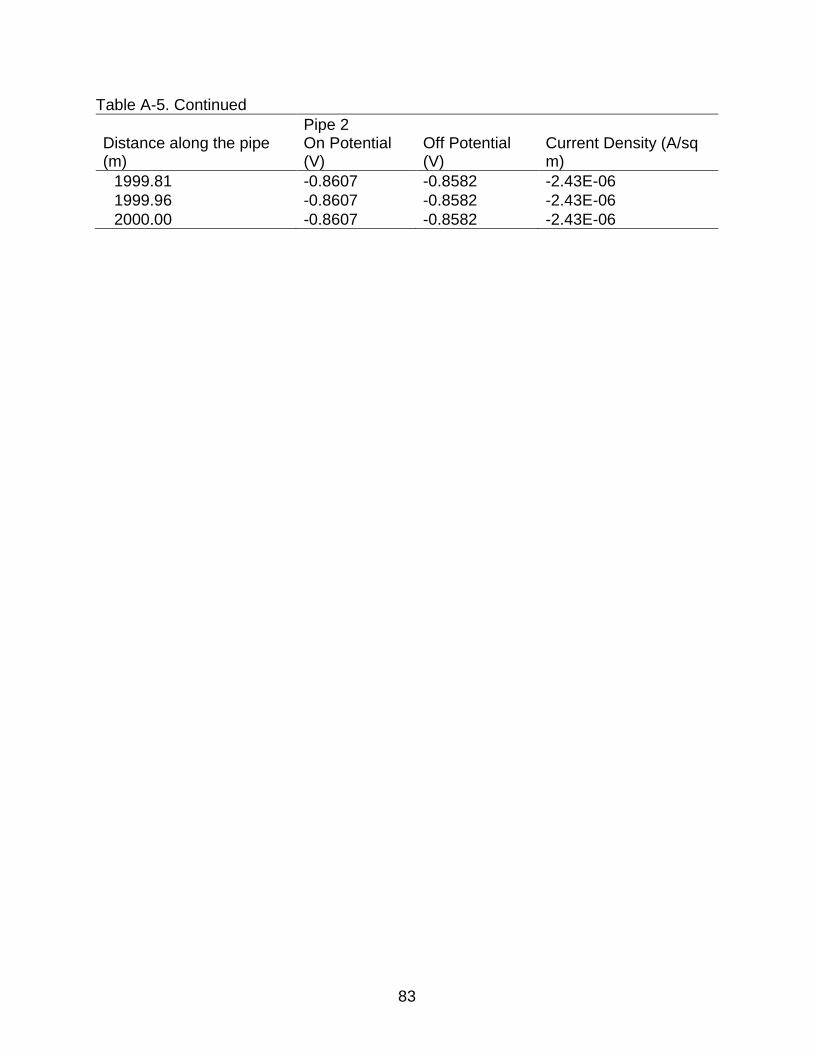
83
Table A-5. Continued
Pipe 2 Distance along the pipe (m)
On Potential (V)
Off Potential (V)
Current Density (A/sq m)
1999.81 -0.8607 -0.8582 -2.43E-06
1999.96 -0.8607 -0.8582 -2.43E-06
2000.00 -0.8607 -0.8582 -2.43E-06
84
LIST OF REFERENCES
[1] D.P. Riemer, Modeling cathodic protection for pipeline networks, University of Florida, Gainesville, 2000.
[2] Pipeline Accident Brief: Blumborough Pennsylvania, National Transportation Safety Board, Washington, D.C., 2008.
[3] P.R. Roberge, Handbook of Corrosion Engineering, McGraw-Hill, 2000.
[4] G.H. Koch, M.P.H. Brongers, N.G. Thompson, Y.P. Virmani, J.H. Payer, Corrosion Cost and Preventive Strategies in the United States, NACE International, CC Technologies Laboratory, United States, 2001.
[5] D.P. Riemer, M.E. Orazem, A mathematical model for the cathodic protection of tank bottoms, Corros. Sci. 47 (2005) 849-868.
[6] E. Santana Diaz, R. Adey, Optimising the location of anodes in cathodic protection systems to smooth potential distribution, Adv. Eng. Software. 36 (2005) 591-598.
[7] E.1. Bardal, I. NetLibrary, Corrosion and protection, Springer, London ; New York, 2004.
[8] J.O. Bockris, M. Gamboa Aldeco, M.E. Gamboa Aldeco, I. NetLibrary, A.K.N. Reddy, Modern electrochemistry. Volume 2A, Fundamentals of electrodics, 2nd edition., Kluwer Academic, New York, 2002.
[9] J. Morgan, Cathodic Protection, 2nd edition, NACE International, Houston, Texas, 1993.
[10] J.S. Newman, Electrochemical Engineering, 2nd edition, Prentice Hall, Englewood Cliffs, New Jersey, 1991.
[11] M.E. Orazem, J.M. Esteban, Phase II Final Report: A Three Dimensional Model for the Cathodic Protection of an Underground Pipeline, Technical Report, University of Florida, 1994.
[12] K. Kennelley, L. Bone, M. Orazem, Current and Potential Distribution on a Coated Pipline with Holidays Part I - Model and Experimental Verification, Corrosion. 49 (1993) 199-210.
[13] D.A. Jones, Principles and Preventions of Corrosion, Prentice Hall, Upper Saddle River, New Jersey, 1996.
[14] M. Orazem, J. Esteban, K. Kenelley, R. Degerstedt, Mathematical Model for Cathodic Protection of an Underground Pipeline with Coating Holidays: Part 1 - Theoritical Development, Corrosion. 53 (1997) 264-272.

85
BIOGRAPHICAL SKETCH
Alok Shankar completed his undergraduate studies in chemical engineering from
National Institute of Technology, Surathkal, India in 2010. He then enrolled at the
University of Florida, Gainesville for the Master of Science program in chemical
engineering in August 2010. He received his Master of Science degree in May 2012.