Buy The Complete Version of This Book at Booklocker.comassets.booklocker.com/pdfs/4514s.pdf · Excel’s consolidation capabilities are limited, ... returning different answers based

An Excel guide for finance and accounting professionals that "cuts to the chase" in fewer than 150 pages, containing top 10 lists for better modeling, reporting, and data analysis... plus macros and userforms. Truly a "must-read" for serious Excel users.

Navigating the Road to EXCEL-lence

Buy The Complete Version of This Book atBooklocker.com:

http://www.booklocker.com/p/books/4514.html?s=pdf


The “Must Read” Excel Guide for Finance and Accounting Professionals

Copyright © 2010 by Eric W. Augusta. All rights reserved

First edition printed January 2010

All rights reserved. Except as permitted by applicable copyright laws, no part of this book may be reproduced, duplicated, sold or distributed

in any form or by any means, either mechanical, by photocopy, electronic, or by computer, or stored in a database or retrieval system

without the express written permission of the publisher, except for brief quotations by reviewers.

ISBN: 978-1-60910-020-9

Printed in the United States of America

This is a work of non-fiction. The ideas presented are those of the author alone. All references to possible income to be gained from the techniques discussed in this book relate to specific past examples and

are not necessarily representative of any future results specific individuals may achieve.

v

TABLE OF CONTENTS

FORWARD ......................................................................................... vii

Chapter 1: 10 “Must Know” Excel FUNCTIONS ............................ 1 Function 1. SUM and “3-D” SUM for Consolidations .......................... 1 Function 2. IF (Plus Logical Functions AND, OR, NOT) .................... 3 Function 3. Conditional Summation ...................................................... 6 Function 4. VLOOKUP ....................................................................... 13 Function 5. CONCATENATION (“&”) .............................................. 17 Function 6. SUBTOTAL (Function) .................................................... 20 Function 7. INDIRECT ........................................................................ 22 Function 8. OFFSET ............................................................................ 24 Function 9. DATE (Year(Ref), Month(Ref), Day(Ref)) ...................... 27 Function 10. TEXT .............................................................................. 27

Chapter 2: 10 “Must Know” Excel FEATURES ........................... 29 Feature 1. Filtering (“Autofilter” in Excel 2003) ................................. 29 Feature 2. Data Validation ................................................................... 31 Feature 3. Conditional Formatting ....................................................... 33 Feature 4. AutoFill ............................................................................... 36 Feature 5. Named Ranges .................................................................... 39 Feature 6. Macro Recorder ................................................................... 45 Feature 7. Goal Seek ............................................................................ 54 Feature 8. Paste Special ....................................................................... 56 Feature 9. Edit, Replace ....................................................................... 58 Feature 10. Forms Controls .................................................................. 60

Chapter 3: Favorite Tips, Tricks, and Shortcuts ........................... 68 Tip 1. My Favorite “Double-Clicks” ................................................... 68 Tip 2. Filling in blank cells .................................................................. 70 Tip 3. The “Camera” Button ................................................................ 71 Tip 4. Creating Multiple Views using VBA to Hide Columns ............ 74 Tip 5. Using Checksums to avoid embarrassing errors ....................... 75 Tip 6. Underling like a pro – choose Font, Single Accounting............ 76

Eric W. Augusta

vi

Tip 7. Using “Very Hidden” worksheets .............................................. 77 Tip 8. Using F5 to delete multiple rows of special cells ....................... 80 Tip 9. The “Rule of 78” ........................................................................ 81 Tip 10. Using the “F4” key ................................................................... 82

Chapter 4: Architecture .................................................................... 85

Chapter 5: A GUIDE TO EXCEL AUTOMATION USING VBA (Visual Basic for Applications) .......................................... 92

About the Author .............................................................................. 133

1

Chapter 1 10 “Must Know” Excel FUNCTIONS

Excel functions are basically predefined formulas. All Excel functions have the same basic layout, which begins with the NAME of the function, followed by a list of ARGUMENTS enclosed in parentheses. With the Analysis ToolPak add-in installed (standard in Excel 2007) there are approximately 350 functions available. This Chapter describes the top 10 functions which I consider most useful for business people, especially when using Excel for financial modeling.

TIP – A fast way to figure out the arguments to be used in a function is to enter the NAME of the function in the formula bar (preceded by the “=” sign) then press “Ctrl” + “a”. This will immediately bring up the INSERT FUNCTION Dialog Box (sometimes referred to as the Formula Palette). This dialog box contains an explanation of each argument along with the proper order for the arguments and a link to the appropriate Help.

Function 1. SUM and “3-D” SUM for Consolidations

SUM is the most used Excel function. If you’re not using it please obtain a basic Excel reference book and read about it. As you do, make sure to understand the various options available for entering arguments, including individual cell references, range addresses and named ranges.

TIP –

Double-click (left mouse button) on the “SIGMA” button [2003 Standard Toolbar, AutoSum button; 2007 Home Ribbon, Edit, AutoSum button) to automatically generate a SUM formula in a cell.

Excel’s consolidation capabilities are limited, in my opinion. The basic choices are:

Eric W. Augusta

2

1) Use Excel’s CONSOLIDATE feature. [2003 Menu Bar, Data, Consolidate; 2007 Data Ribbon; Data Tools, Consolidate]

2) Create a formula using the “+” operator along with a series of specific cell / sheet references, or

3) Create a “3-D SUM” formula.

After trying all of these, I prefer the “3-D SUM” approach. It works by summing cells across sheets that are physically located BETWEEN and INCLUDING sheets referenced in the formula. For example, the formula “= SUM (Sheet1:Sheet5!D3)” will result in the addition of the contents of cell D3 on Sheet1, Sheet5, and all sheets physically located between Sheet1 and Sheet5 in the workbook.

The key benefits of this approach are simplicity, flexibility, and the fact it is DYNAMIC. My favorite technique is to create two “dummy” blank sheets, e.g. Sheet “A” and Sheet “Z”, located at either end of the sheets to be consolidated. The formula can then be set up as follows “= SUM(A:Z!C4)”. This formula will NOT need to be changed when sheets are added or deleted between sheets “A” and “Z”.

Example (where cell C4 on sheets “Division1”, “Division2”, and “Division3” is = 5).

When using this formula it’s important the row and column structures on each consolidated and the summary sheet are identical. If not, summing all the “C4” cells (in the example) may not produce a meaningful result.

When using this “3-D SUM” technique, exercise caution when adding or deleting rows or columns to the consolidating and summary sheets. In order for the consolidating formulas to automatically adjust, ALL


3

consolidating sheets AND the summary sheet must be selected (“grouped”) before the columns and/or rows are added or deleted.

Function 2. IF (Plus Logical Functions AND, OR, NOT)

“IF” functions are indispensable for building most financial models. They provide “intelligence” to distinguish between alternative conditions, returning different answers based on criteria set up in the IF formula. An IF formula has three arguments:

1) The Logical Test 2) The Value to be returned if the Logical Test is TRUE

and 3) The Value to be returned if the Logical Test is FALSE.

If we refer to these three arguments as A, B, and C, then a simple phrase captures the logic involved: “If A is True, then do B, otherwise do C”.

The six basic logic tests that can be used in the A portion of the arguments include Equal to (=), Greater Than (>), Less Than (<), Greater Than or Equal to (>=), Less Than or Equal to (<=), and Not Equal to (<>).

In the “A” portion (the logical test) Excel allows the use of numbers, text, or dates as criteria for testing. If text is used, it must be an exact match except for case, so be careful about extraneous spaces or characters. The criteria for testing in the A portion may be either entered directly in the formula, or referred to as external cells / ranges.

For example, the formula =IF(SUM(A1:A5)<0,”Sum is Negative”, SUM(A1:A5)) will return a text answer of “Sum is Negative” if the sum is negative, otherwise it will return the sum of range A1:A5.

Logical Functions AND, OR, NOT can be combined with IF formulas:

Excel allows the user to create what are called Logical formulas. The three functions that fall into this category are =AND(Test1,Test2, etc.),

Eric W. Augusta

4

=OR(Test1,Test2,etc.), and =NOT(Test1 argument only). The result of a Logical (sometimes called a Boolean) function is either TRUE or FALSE.

Example: = AND(A1=2, A2=3) will produce TRUE only if BOTH A1=2 and A2=3. Any other condition will produce FALSE

Example: = OR(A1=A2, D5=D6, F4=F5) will produce TRUE if ANY of the three logical tests are true.

Example: = NOT(A1=4) will produce TRUE if A1 is NOT equal to 4, and FALSE if A1 IS equal to 4.

Combining one of these with an IF formula is easy. Just think of any of the above three examples as replacing the entire “A” section of an IF statement. In this way you create an IF statement that meets the requirement of the “A” section, as being evaluated to a TRUE or a FALSE condition.

Example = IF(AND(A1=2, A2=3),”GO”, “STOP”) will return “GO” if the AND logical function is TRUE, and “STOP” if the AND logical function is FALSE.

“Nested” IF statements.

A “nested” IF formula is one where a second (or third, or fourth, up to a seventh in Excel 2003 or a 64th in Excel 2007) IF statement is inserted INSIDE the first statement’s “B” and/or “C” portion. This allows the formula to encompass multiple conditions. An example of a single level nested IF statement would be this formula for determining the grade, based on the score value:

Scores 8-10 = Excellent Scores 6-7 = Good Scores 0-5 = Fair


5

As you can see, this formula is complex to create with only ONE level of nesting. Imagine seven or more levels, if you can. And, these formulas can be very difficult to edit later on. For these reasons, I strongly recommend NOT using nested IF statements unless absolutely necessary. The alternative approach I recommend is a VLOOKUP table. The advantages are:

1) Easier to construct

2) Easier to edit the formula if necessary, and

3) Variables can be changed in the table WITHOUT having to modify the formula! The example below can replace the previous nested IF formula. For more on VLOOKUPS, please see below.

Eric W. Augusta

6

Function 3. Conditional Summation

SUMIF( 1 condition, Excel 2003 and Excel 2007)

SUMPRODUCT, DSUM ( multiple conditions, Excel 2003 and Excel 2007)

SUMIFS (multiple conditions, Excel 2007 only)

SUMIF is one of my favorite functions. It sums a range of cells, BASED ON A CRITERION. The syntax is:

=SUMIF(Evaluation Range, Criterion, Sum Range)

As you can guess, if the criterion in cell A9 is not an EXACT match to any cells in the Evaluation Range (excluding capitalization), an incorrect result can occur. One method to eliminate this problem is the create cell A9 as a DATA VALIDATED cell (see Features Chapters of book), using List Validation and referencing a separate list of valid criteria.

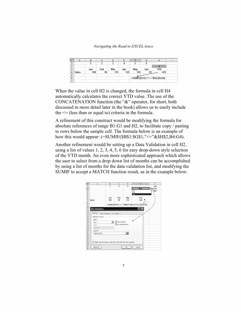
Another important, and sometimes overlooked aspect of the SUMIF function is its ability to recognize other logical operators, specifically >, <, <=, >=, and <>. Combining this with using SUMIF on a horizontal orientation allows us to create a clever method for automatically calculating YTD numbers in financial schedules. The following example shows how:


7

When the value in cell H2 is changed, the formula in cell H4 automatically calculates the correct YTD value. The use of the CONCATENATION function (the “&” operator, for short, both discussed in more detail later in the book) allows us to easily include the <= (less than or equal to) criteria in the formula.

A refinement of this construct would be modifying the formula for absolute references of range B1:G1 and H2, to facilitate copy / pasting to rows below the sample cell. The formula below is an example of how this would appear: (=SUMIF($B$1:$G$1,”<=”&$H$2,B4:G4).

Another refinement would be setting up a Data Validation in cell H2, using a list of values 1, 2, 3, 4, 5, 6 for easy drop-down style selection of the YTD month. An even more sophisticated approach which allows the user to select from a drop down list of months can be accomplished by using a list of months for the data validation list, and modifying the SUMIF to accept a MATCH function result, as in the example below:

Eric W. Augusta

8

Range Naming of the Criteria Range is also a good idea since this eliminates the need for using absolute references and makes the formula more readable. Other refinements include hiding the criteria row for aesthetic reasons, using Row, Hide or Data Group, and Outline.

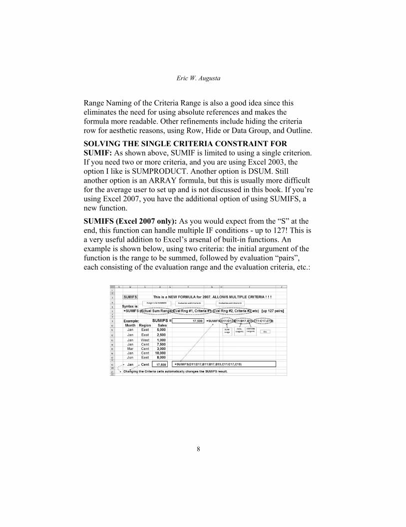
SOLVING THE SINGLE CRITERIA CONSTRAINT FOR SUMIF: As shown above, SUMIF is limited to using a single criterion. If you need two or more criteria, and you are using Excel 2003, the option I like is SUMPRODUCT. Another option is DSUM. Still another option is an ARRAY formula, but this is usually more difficult for the average user to set up and is not discussed in this book. If you’re using Excel 2007, you have the additional option of using SUMIFS, a new function.

SUMIFS (Excel 2007 only): As you would expect from the “S” at the end, this function can handle multiple IF conditions - up to 127! This is a very useful addition to Excel’s arsenal of built-in functions. An example is shown below, using two criteria: the initial argument of the function is the range to be summed, followed by evaluation “pairs”, each consisting of the evaluation range and the evaluation criteria, etc.:


9

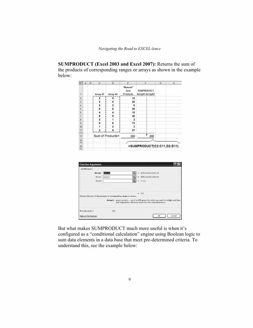
SUMPRODUCT (Excel 2003 and Excel 2007): Returns the sum of the products of corresponding ranges or arrays as shown in the example below:

But what makes SUMPRODUCT much more useful is when it’s configured as a “conditional calculation” engine using Boolean logic to sum data elements in a data base that meet pre-determined criteria. To understand this, see the example below:

Eric W. Augusta

10

The secret to this formula is the use of Boolean logic to determine if each element in the Region array is equal to the criterion cell C13 (“West”), and if it is, the Boolean result of TRUE is equal to a value of 1.

If FALSE, the value is 0. Only instances where “TRUE” times “TRUE” exist (“West” AND “B”) will multiplication of the column E array yield a non-zero result. Adding additional conditions beyond the two shown is a relatively straightforward exercise, which I leave to the reader to explore. About the only “downside” I’ve found to using SUMPRODUCT in this way is it isn’t as efficient as using the DSUM approach, described next. So for those readers where performance is an issue, DSUM may be a better solution.

DSUM:

Excel offers 12 database functions - DAVERAGE, DCOUNT, DCOUNTA, DGET, DMAX, DMIN, DPRODUCT, DSTDEV, DSTDEVP, DSUM, DVAR, and DVARP - to retrieve data from a table or database. DSUM, as its name suggests, allows you to sum selected data members within the data base, according to multiple criteria.

DSUM requires three arguments:

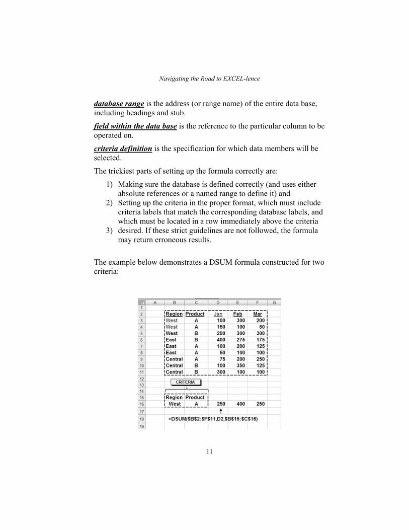
=DSUM (database range, field within the data base, criteria definition)


11

database range is the address (or range name) of the entire data base, including headings and stub.

field within the data base is the reference to the particular column to be operated on.

criteria definition is the specification for which data members will be selected.

The trickiest parts of setting up the formula correctly are:

1) Making sure the database is defined correctly (and uses either absolute references or a named range to define it) and

2) Setting up the criteria in the proper format, which must include criteria labels that match the corresponding database labels, and which must be located in a row immediately above the criteria

3) desired. If these strict guidelines are not followed, the formula may return erroneous results.

The example below demonstrates a DSUM formula constructed for two criteria:

Eric W. Augusta

12

Note the use of absolute references ($ signs) for the database range ($B$2:$F$11) and for the criteria range ($B$15:$C$16). This facilitates copying the formula to the right. This example can easily be expanded to three, four, five or more criteria by simply expanding the database and criteria ranges as appropriate to accommodate additional columns, such as adding a Salesperson column between columns B and C and adjusting the criteria range.

Another interesting use of the DSUM function is for summing across dates (or other values) that are within certain criteria parameters, using the standard >, <, <=, >=, <> logical comparisons. By including logical operators in the criteria (using concatenation with the symbols entered into cells A11 and B11) as shown below, this example shows how it is possible to sum only those amounts for dates that are greater than 1/11/10 AND less than or equal to 2/25/10.


13

Function 4. VLOOKUP

VLOOKUP for vertical tables (and HLOOKUP for horizontal tables) can be used to find data stored in a table. Its usefulness becomes obvious when you consider the alternative ─ a “nested” IF statement ─ which is cumbersome to create and difficult to edit.

The syntax for the VLOOKUP consists of four arguments, with the fourth argument (range lookup) being optional:

=VLOOKUP (lookup value, lookup table, lookup table column number, range lookup)

lookup value is the value, or reference to a cell containing the value, to be looked up in the table’s LEFTMOST COLUMN.

lookup table is the range that defines the entire table, including the leftmost column that contains the values being looked up. For example, the range of the table might be B6:F15, which defines a table five columns wide by ten rows down. Another more common way is to refer to tables by previously applying a NAMED RANGE to the entire table, then referring to this named range in the argument.

lookup table column number is the number of the column where the answer will be found. VLOOKUP tables have their columns numbered from left to right, starting with the first column on the left, designated as column 1.

range lookup is either TRUE or FALSE, and if nothing is entered, the default assumed is TRUE. If TRUE or nothing is entered for this argument, the lookup value is “scanned” down column 1 until the closest match without exceeding the lookup value is found.

At this point, the function moves over to the lookup table column number and finds the corresponding data element located in the cell of this column that is on the same row as the lookup value.

NOTE: for this to work, the lookup values in column 1 must be sorted in ascending sequence either by number values, date values, or text alphabetically.

Eric W. Augusta

14

For example:

If a non-exact match lookup value is entered, e.g. 2.3 with a TRUE or default range lookup, the result will be unchanged, since the value 2.3 is between 2 and 3 in column 1, which is being scanned for the match. But if a non-exact match lookup value is entered (e.g. 2.3) with a FALSE range lookup, the result will be an error (#N/A), since 2.3 isn’t found exactly in column 1.

Dealing with a #N/A error result for a VLOOKUP is often a major problem, since this can cause a “ripple effect” of errors throughout a spreadsheet. A simple solution is to combine the VLOOKUP with an IF statement that “traps” such an error before it can cause a problem. The secret to this formula is the ISERROR function, which returns TRUE if a #N/A answer is the result. Modifying the previous VLOOKUP as


15

follows will correct the problem by inserting a zero answer instead of the error. Note that in Excel 2007, a new function is available - IFERROR - that allows the user to create a simpler formula that achieves the same result, requiring only two arguments, the result if an error, the result if not an error.

Example [Excel 2003] =IF(ISERROR(VLOOKUP(A1,A3:C15,3,FALSE)),0,VLOOKUP(

A1,A3:C15,3,FALSE))

Example [Excel 2007] =IFERROR(VLOOKUP(A1,A3:C15,3,FALSE),0)

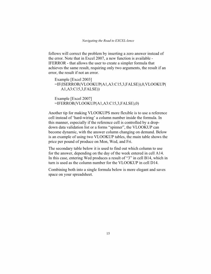
Another tip for making VLOOKUPS more flexible is to use a reference cell instead of ‘hard-wiring’ a column number inside the formula. In this manner, especially if the reference cell is controlled by a drop-down data validation list or a forms “spinner”, the VLOOKUP can become dynamic, with the answer column changing on demand. Below is an example of using two VLOOKUP tables, the main table shows the price per pound of produce on Mon, Wed, and Fri.

The secondary table below it is used to find out which column to use for the answer, depending on the day of the week entered in cell A14. In this case, entering Wed produces a result of “3” in cell B14, which in turn is used as the column number for the VLOOKUP in cell D14.

Combining both into a single formula below is more elegant and saves space on your spreadsheet.

Eric W. Augusta

16

A final note – some excellent applications for using VLOOKUP (or HLOOKUP) include:

1) Commission Plan calculations, e.g. enter Sales, lookup commission percent rate

2) Tax Tables, e.g. enter Taxable Income, lookup marginal percent tax rate

3) Inventory data lookups, e.g. enter part number, lookup Qty, Price, Status, etc.

A major shortcoming for VLOOKUP formulas is the requirement for using the LEFTMOST column of the table as the VLOOKUP column.

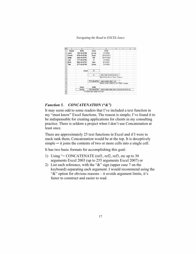
If this is not possible, or inconvenient to set up, consider setting up a simple combination of INDEX and MATCH functions.

The example below demonstrates using MATCH and INDEX to use the ‘Dept’ column for the lookup and the ‘SSN’ column for the answer.


17

Function 5. CONCATENATION (“&”)

It may seem odd to some readers that I’ve included a text function in my “must know” Excel functions. The reason is simple; I’ve found it to be indispensable for creating applications for clients in my consulting practice. There is seldom a project when I don’t use Concatenation at least once.

There are approximately 25 text functions in Excel and if I were to stack rank them, Concatenation would be at the top. It is deceptively simple ─ it joins the contents of two or more cells into a single cell.

It has two basic formats for accomplishing this goal:

1) Using “= CONCATENATE (ref1, ref2, ref3, etc up to 30 arguments Excel 2003 (up to 255 arguments Excel 2007) or

2) List each reference, with the “&” sign (upper case 7 on the keyboard) separating each argument. I would recommend using the “&” option for obvious reasons – it avoids argument limits, it’s faster to construct and easier to read.

Eric W. Augusta

18

Example of joining the contents of three cells together (both formats):

A caveat when using Concatenation ─ If numbers (values) are concatenated, they will be converted to text. To convert back to a value, either use the =VALUE function, multiply the result by 1, add zero to the result, or divide the result by one.

Example:

I often describe concatenation as a way to create “Smart Text”. This means creating what looks like text on a printed page, but which has the ability to calculate like an arithmetic formula ─ which it is! An example is shown below:


19

Company ABC’s financial model lists key assumptions in a separate area of the financial statements sheet, and management would like to see these assumptions replicated on the stub of the financial statements, as appropriate. But to avoid having to retype the financial statement stubs to reflect assumptions changes, “Smart Text” concatenation may be used.

If cell B3 is changed to 50 percent, this will automatically be reflected in cell A13’s result. This example brings up another important characteristic of concatenation ─ when formatted numbers are included in a concatenation formula, any previous number formatting is “lost”. In the above example, this means that the 45 percent value would appear in the concatenated cell A13 as simply 0.45. To fix this, we have two basic options:

1) Use arithmetic operations in the formula to convert the number scale to what is required (multiplying by 100 converts the 0.45 to 45) and then concatenate the missing “percent” ending to the 45 result, or

2) Use the TEXT function, a more elegant and flexible approach, but

one that also requires the user to have some knowledge of formatting codes ($, percent, ###, 0.0, etc). If the reader is comfortable with using these codes, then this is my recommended approach. The TEXT function is described in more detail later in this book as #10 in the list of “Must Know” Excel functions.

Eric W. Augusta

20

Other uses of concatenation:

1) Including a master, variable date into various related financial schedules that require the date to be part of the schedules title, heading, stub etc.

2) Calculating “footnotes” in financial reports, that automatically reflect any changes made to key schedules in the report.

Other Text Functions with which the reader may want to become familiar are LEFT, MID, RIGHT, SUBSTITUE and REPLACE, all described in most Excel reference books.

Function 6. SUBTOTAL (Function)

A common situation that confronts many finance and accounting professionals is a financial spreadsheet that contains various subtotal rows. Making sure the grand total does NOT double-count any of the subtotals can be a problem, but not if using the SUBTOTAL function, which automatically ignores any other SUBTOTAL functions within its range of summation arguments. In addition, it will ignore hidden rows


21

in a filtered list, another extremely powerful aspect of the SUBTOTAL function.

The SUBTOTAL’s syntax is:

= SUBTOTAL [function code, ref1, ref2, ref 3, etc up to 29 maximum (Excel 2003) or 254 (Excel 2007)].

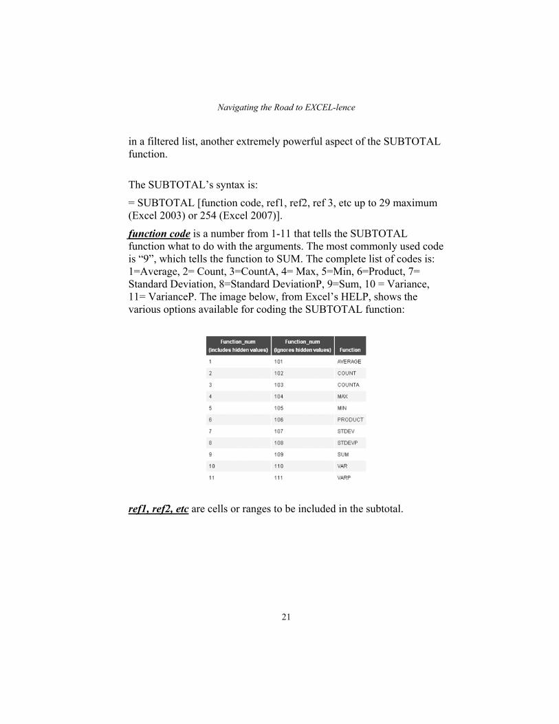
function code is a number from 1-11 that tells the SUBTOTAL function what to do with the arguments. The most commonly used code is “9”, which tells the function to SUM. The complete list of codes is: 1=Average, 2= Count, 3=CountA, 4= Max, 5=Min, 6=Product, 7= Standard Deviation, 8=Standard DeviationP, 9=Sum, 10 = Variance, 11= VarianceP. The image below, from Excel’s HELP, shows the various options available for coding the SUBTOTAL function:

ref1, ref2, etc are cells or ranges to be included in the subtotal.

Eric W. Augusta

22

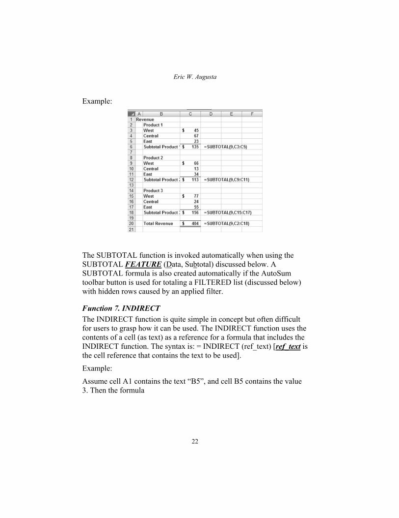
Example:

The SUBTOTAL function is invoked automatically when using the SUBTOTAL FEATURE (Data, Subtotal) discussed below. A SUBTOTAL formula is also created automatically if the AutoSum toolbar button is used for totaling a FILTERED list (discussed below) with hidden rows caused by an applied filter.

Function 7. INDIRECT

The INDIRECT function is quite simple in concept but often difficult for users to grasp how it can be used. The INDIRECT function uses the contents of a cell (as text) as a reference for a formula that includes the INDIRECT function. The syntax is: = INDIRECT (ref_text) [ref_text is the cell reference that contains the text to be used].

Example:

Assume cell A1 contains the text “B5”, and cell B5 contains the value 3. Then the formula


23

= INDIRECT (A1) would return 3, which is the contents of cell B5, which is the text reference contained in cell A1. This is obviously simplistic and of little value when constructed in this manner.

Let’s now examine three other practical applications of INDIRECT:

1) Using INDIRECT to access different VLOOKUP tables, depending on the range name selected in cell C11 (data validated cell to ensure only appropriate named ranges are selected).

An enhancement to this construct would be a separate table of Sales Reps, listing which are either “Jr” or “Sr”, and the appropriate named range table to use, thus eliminating the need to select the correct Rate Table in cell D11 (which would instead contain a formula such as = VLOOKUP(C11,TableReps,2,False)).

2) Use INDIRECT to create a two-level set of Data Validated cells, the second cell being dependent on the category selected in the first cell. In this situation, INDIRECT is used to define the appropriate LIST to be used in the Level 2 Data Validated Cell, which is dependent upon the selection made in the Level 1 cell, which uses the range “Spares” for its list.

Eric W. Augusta

24

3) Use INDIRECT to create Consolidating formulas that reference

sheets as text in cells B3, B5, B7 and the sheet level named range “Sales” entered as text in cell E1.

A side note on syntax – if you are using the more standard A1 reference system, the syntax above is fine. If you are using the R1C1 system, then you must include FALSE after the ref_text (separated with a comma) to let the function know to employ that system. The default is TRUE (A1) if omitted.

Function 8. OFFSET

The offset function allows you to refer to a location that is “offset” from a reference location. The syntax is:

= OFFSET (reference, rows offset from reference, columns offset from reference, height of new location, width of new location).


25

reference is the range or cell upon which the offset will be defined.

rows offset is the number of rows up (positive integer) or down (negative integer) for the offset.

columns offset is the number of columns to the right (positive integer) or left (negative integer) for the offset.

height (optional, default is 1) is the number of rows (positive integers only) to be returned.

width (optional, default is 1) is the number of columns (positive integers only) to be returned.

The OFFSET function can be used in several interesting ways. Three examples:

1) As a stand-alone function to return the value of the cell that is located “r” rows and “c” columns from the reference cell,

2) As a function INSIDE another function in order to return a range that the other function is expecting,

3) to create a dynamic named range, allowing the user to create charts, list boxes, combo boxes, etc. that automatically adjust for changes in the number of data input rows or columns.

Example 1:

Using OFFSET as a standalone function, each Revenue (invoice) amount can be offset to the right the number of months entered in cell B5.

Eric W. Augusta

26

Example 2:

Using OFFSET inside the SUM function allows for variable summation of the months, based on the YTD month entered in cell G2, since the OFFSET function is now returning a variable range.

Example 3:

Using OFFSET to define a named range (Insert, Name, Define) allows a Forms Control List Box to automatically adjust for variable numbers of data elements in the source list. The COUNTA part of the OFFSET formula is setting a variable HEIGHT, based on the count of names in column A. The fifth argument (Width) has been omitted, defaulting to 1.


27

Function 9. DATE (Year(Ref), Month(Ref), Day(Ref))

The DATE function is used to return a serial date, using the three arguments of Year, Month, and Day, each entered as integers. See the examples below for use of this function to create serial dates using inputs from three cells.

The Year, Month, and Day can be entered in separate cells, and using the DATE function, combined to create a serial date. These separate cells may be controlled with a Spinner or a Scroll Bar for easily changing dates across a wide range of values.

Function 10. TEXT

The TEXT function uses the syntax TEXT (value, format_text),converts a numeric value to text and allows you to specify

Eric W. Augusta

28

the display formatting by using the same formatting codes that are available for custom cell formatting.

The TEXT function is most important in modeling when used in conjunction with CONCATENATION to form “Smart Text”, or formulas that print to look like text.

The examples below illustrate the usefulness of this function when creating more complex financial models:

The primary requirement for the effective utilization of the TEXT function is an understanding of the formatting codes in Excel. Complete lists of these are available in most every Excel reference book as well as in on-line HELP.

An Excel guide for finance and accounting professionals that "cuts to the chase" in fewer than 150 pages, containing top 10 lists for better modeling, reporting, and data analysis... plus macros and userforms. Truly a "must-read" for serious Excel users.


Buy The Complete Version of This Book atBooklocker.com:

http://www.booklocker.com/p/books/4514.html?s=pdf

Documents

Buy The Complete Version of This Book at Booklocker.comassets.booklocker.com/pdfs/4514s.pdf · Excel’s consolidation capabilities are limited, ... returning different answers based