Embed Size (px)
Citation preview

Business Strategies Towards the
Creation, Absorption and Dissemination
of New Technologies
Dissertation
zur Erlangung des akademischen Grades
eines Doktors
der Wirtschafts- und Sozialwissenschaften
(Dr. rer. pol.)
des Departments Wirtschaftswissenschaften der
Universität Hamburg
von Lars Wiethaus
Hamburg, Juni 2005

Mitglieder der Promotionskommission
Vorsitzender: Prof. Dr. Manfred Holler
Erstgutachter: Prof. Dr. Wilhelm Pfähler
Zweitgutachter: Prof. Dr. Stefan Napel
Das wissenschaftliche Gespräch fand am 2. November 2005 statt.

Meinen Eltern

Preface
This cumulative thesis comprises four theoretical papers related to business strategies towards the creation, absorption and dissemination of new technologies.
The first paper “Absorptive Capacity and Connectedness: Why
Competing Firms also Adopt Identical R&D Approaches” is published in the International Journal of Industrial Organization, 23 (2005) 467-481. The Elsevier Science B.V. copyright is acknowledged. The
paper was presented at the “European Summer School on Industrial
Dynamics” (ESSID 2003), ZEW and University of Bocconi, in Corse.
The second paper “Cooperation or Competition in R&D When
Innovation and Absorption Are Costly” is forthcoming in Economics of Innovation and New Technology, 2006. I acknowledge the Taylor and Francis copyright. This paper was presented at the conference
‘Industrial Organization and Innovation’, INRA and GEAL, in
Grenoble and at the ‘Jahrestagung 2005’, Verein für Socialpolitik, in Bonn.
The third paper “Excess Absorptive Capacity and the Persistence of
Monopoly” was presented at ‘EARIE 2005’, European Association of
Research in Industrial Economics, in Porto, the ‘2nd ZEW Conference
on Innovation and Patenting’, ZEW, in Mannheim and the annual meeting of the German Association of Business Administration
(GEABA), ‘VI. Symposium zur ökonomischen Analyse der
Unternehmung’, in Freiburg.
The fourth paper “Knowledge Transfer in Buyer-Supplier
Relationships – When It (Not) Occurs” is the result of joint research
with Werner Bönte. The paper was presented at ‘EARIE 2005’, European Association of Research in Industrial Economics, in Porto and the annual meeting of the German Association of Business
Administration (GEABA), ‘VI. Symposium zur ökonomischen
Analyse der Unternehmung’, in Freiburg.
Hamburg, November 2005 Lars Wiethaus

Acknowledgements
I would like to thank Wilhelm Pfähler for his invaluable comments and guidance. I am also grateful to the other members of the committee, Stefan Napel and Manfred Holler, for reading and commenting on this thesis. I benefited considerably from discussions
with Werner Bönte, and would like to thank him for insightful comments and suggestions. Moreover Tom Gresik provided very helpful comments.
Many other people have contributed. Thanks are due, in particular,
to Johannes Bruder, Ludwig Burger, Heidrun Hoppe, Björn Möller, Stephan Tolksdorf and participants of seminars at the University of Hamburg and several conferences.
Finally I am indebted to Nina Carlsen for her support, encouragement and constant willingness to discuss the meaning and the purpose of my work.
Hamburg, November 2005 Lars Wiethaus

Contents
General Introduction
Absorptive Capacity and Connectedness:
Why Competing Firms also Adopt
Identical R&D Approaches
Cooperation or Competition in R&D
When Innovation and Absorption
Are Costly
Excess Absorptive Capacity and the
Persistence of Monopoly
Knowledge Transfer in
Buyer-Supplier Relationships
- When It (Not) Occurs
(with Werner Bönte)

General Introduction

1 Creation, Absorption and Dissemination of
New Technologies
In high-tech industries the creation of new technologies is the most impor-
tant origin of competitive advantage. At the same time, new technologies,
developed by one’s competitor, constitute the most severe threat to a firm’s
established market position. Not surprisingly high-tech firms invest substan-
tial amounts of money in research and development (R&D), i.e. up to 15.5 %
of sales1 in the pharmaceuticals & biotechnology sector as well as in the IT
hardware sector. R&D expenditures in the five most R&D intensive sectors
amount to a fivefold of companies’ dividends2. The decision on the optimal
R&D budget as well as its allocation to certain activities becomes, as Baumol
(2002) puts it, “a matter of life and death” for many firms. These decisions
are notably complex for at least two reasons. The first, rather general one,
arises from strategic behavior in high tech industries. The second reason is
due to the specific properties of new technologies. We shall briefly deal with
each point.
With respect to strategic behavior, Leahy and Neary (1997) note that
“since R&D is a component of fixed costs, industries where it is important
tend to be concentrated”. Indeed the bulk of R&D, in absolute terms, is
undertaken by firms with high market shares (Scherer 1967, Blundell and
Griffith 1998). By the same token most and major innovations are generated
by dominant firms (e.g. Sorescu et al. 2003). In concentrated, oligopolistic
industries one firm’s creation of a new technology, say the introduction of a
faster microprocessor, materially affects other firms’ demand and profitabil-
ity respectively. Being aware of this fact firms need to make their decisions
in anticipation of a competitor’s likely action as well as under consideration
of competitors’ responses. Between 2001 and 2003 the microprocessor manu-
1European Commission, "Monitoring industrial research: the 2004 EU industrial R&Dinvestment scoreboard".
2DTI, "The 2004 R&D Scoreboard. The top 700 UK and 700 international companiesby R&D Investment", www.innovation.gov.uk. Geroski et al. (1993), Bayus et al. (2003)and Sorescu et al. (2003) provide empirical studies on the relationship between innovationand firm profitability.
1

facturer AMD, for instance, devoted about 2.3 billion US $ to R&D (15% to
30% of sales) while having summed up losses of more than 1.5 billion3. Such
aggressive R&D investments would be rather unlikely in absence of Intel’s
progress and the threat of falling behind the technological edge. In this re-
spect, however, investments in new technology creation do not seem to differ
from any other sort of fixed costs, like investments in capacity.
What distinguishes an investment in new technology creation, e.g. R&D
investments, essentially from an investment in tangible assets is that new
technologies comprise, to some extent, the properties of a public good4. A
public good is both nonrival, i.e. its use by one person does not preclude its
use by another person, and nonexcludable, i.e. the owner of a good cannot
prevent others from using it. New technologies are nonrival in the sense that
“once the cost of creating a new set of instructions has been incurred, the
instructions can be used over and over again at no additional cost” (Romer
1990).
The extent to which new technologies are nonexcludable depends on the
nature of the technology in question and the legal system. For instance new
technologies as an outcome of basic research are less excludable as compared
to those that arise from solving a firm specific problem. The legal system
of patent and property rights protection, too, varies across countries and in-
dustries, being notably strong in the pharmaceutical and chemical industry
and rather weak in the semiconductor or biotechnology industry (e.g. Cohen
et al. 2000). Nonexcludabilities in new technology creation are commonly
expressed as technology or knowledge spillovers which “include any original,
valuable knowledge generated in the research process which becomes pub-
licly accessible, whether it be knowledge fully characterizing an innovation,
or knowledge of a more intermediate sort” (Cohen and Levinthal 1989). Im-
portant channels of spillovers are fluctuations of scientists or information that
has to be made public in order to commercialize a new technology (Mansfield
1985).
As a consequence of technological spillovers firms cannot appropriate all
3See annual reports, www.amd.com.4A second fundamental difference is that the outcome of R&D is uncertain which is,
however, not the focus of this thesis.
2

of their R&D efforts exclusively (Nelson 1959, Arrow 1962, Spence 1984)
which further complicates R&D related decisions. In particular it may be
profitable to reduce investments in new technology creation as compared to
a situation in which a firm’s own efforts would not simultaneously enhance
the competitiveness of its rival. Indeed, Jaffe (1998) stresses the implicit con-
nection between spillovers and strategic R&D reduction: “proponents and/or
reviewers will cite the diffuse and high-risk nature of the potential benefits
as reasons why private capital is not forthcoming, or note that the project
is not part of the proponent’s core business”. As an indicator of the impor-
tance of spillovers for R&D investments empirical literature as summarized
by Griliches (1992) suggests a spillover level5 between 50% and 100% relative
to private R&D investments within the industrial sector. Having said this,
spillovers are not exogenously given for a firm but determined by additional
actions, namely efforts to absorb and the firm’s willingness to disseminate
new technologies.
Efforts to absorb new technologies are necessary because the latter do not
rain “down upon its beneficiaries like manna from heaven, [in the sense that]
no effort is needed of the recipients, not even purchase of a bucket” (Kamien
and Zang 2000). Rather firms need the ability “to identify, assimilate and
exploit existing information”, i.e. absorptive capacity. In this context Cohen
and Levinthal (1989) highlighted the ‘second face’ of R&D: learning. That is,
besides the incentive to generate innovations, firms also seek to improve their
absorptive capacity. Anecdotal6 as well as empirical7 evidence support the
relevance of absorptive capacity as a second motivation for R&D investments.
However, the absorption of externally developed new technologies does
not (necessarily) require R&D efforts in terms of an own innovation. Empir-
ical studies8 indicate that absorption requires specific R&D efforts to imitate
5Measured as the gap between the social rate of return and the private rate of return onR&D investments. The spillover rates of Table 1 in Griliches (1992, p. S43) are expressedas the excess of the social rate of return with respect to the private rate of return (relativeto the social rate of return). Jaffe (1986) provides an early study on the importance ofknowledge spillovers.
6See Cohen and Levinthal (1989, 1990) and the work cited.7See Griffith et al. (2003).8See “Cooperation or Competition in R&D When Innovation and Absorption Are
3

(rather than to innovate). As a consequence firms need to adjust their deci-
sions towards new knowledge creation with respect to both their rivals’ likely
innovation and absorption efforts. The paper “Cooperation or Competition
in R&D When Innovation and Absorption Are Costly” analyzes firms’ si-
multaneous decisions with respect to innovation and absorption. The paper
“Excess Absorptive Capacity and the Persistence of Monopoly” addresses
the question how an incumbent firm may utilize its absorptive capacity as a
means to discourage a potential entrant’s innovation efforts and consequently
entry.
Yet technological spillovers are not exclusively described through a firm’s
involuntary leakage of knowledge and another firm’s efforts to absorb this
knowledge. In addition firms may have an incentive to stimulate the dis-
semination of new technologies. In the case of vertically related firms, i.e.
buyer-supplier relationships, the incentive for new technology dissemination
occurs because this usually increases the efficiency of the buyer-supplier rela-
tionship. Moreover, at first glance, firms do not risk the loss of a competitive
advantage in vertical relationships. Yet this paints only half the picture if a
supplier, for instance, maintains relationships with additional buyers. Then
each buyer needs to trade off efficiency gains from knowledge dissemination
against the threat of technology transfer through a common supplier (see the
paper “Knowledge Transfer in Buyer-Supplier Relationships - When It (Not)
Occurs”).
If firms are horizontally related, incentives for knowledge dissemination
are less straightforward because competitive advantages, in general, are tied
to technological advantage. However one may think of two reasons why
also competing firms may foster knowledge flows. Provided these flows are
sufficiently reciprocal (von Hippel 1987) firms are better off through the ex-
change of knowledge as compared to an individual creation of knowledge.
Furthermore knowledge dissemination frees firms from the above sketched
dilemma of aggressive R&D investments: if the dissemination of new tech-
nologies is guaranteed there hardly exists any pressure of creating them in
the first place. The practice of horizontal knowledge dissemination is well
documented through case evidence of von Hippel (1987), Schrader (1990) and
Costly” for an overview.
4

Baumol (2001) but has not been explained theoretically9. The paper “Ab-
sorptive Capacity and Connectedness: Why Competing Firms also Adopt
Identical R&D Approaches” deals with that question.
2 Purpose and Contributions
This thesis aims to identify and to close some gaps in the literature dealing
with business strategies towards the creation, absorption and dissemination
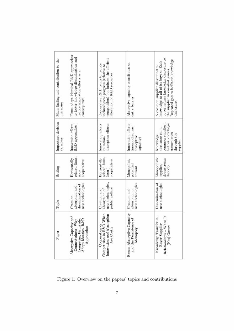
of new technologies. In doing so it comprises four theoretical papers. The
following abstracts and Figure 1 briefly link each paper to one ore more of the
above mentioned topics (creation, absorption and dissemination) and report
its main findings and contributions to the literature. For further details the
reader is referred to the particular paper.
Absorptive Capacity and Connectedness: Why Competing Firmsalso Adopt Identical R&D Approaches10 This paper explores firms’
decisions regarding the dissemination and absorption of new technologies as
well as their creation. In particular firms determine both the dissemination
and absorption through their choices of R&D approaches. Whereas identical
(broad) R&D approaches ‘connect’ firms with their R&D environment and
maximize knowledge dissemination and absorptive capacities, the opposite
holds for idiosyncratic R&D approaches. The model shows that competing
firms choose identical R&D approaches in order to maximize knowledge flows
between each other. In essence, this frees firms from the dilemma of aggres-
sive investment in R&D. Our analysis contrasts with Kamien and Zang’s
(2000) finding that competing firms chose idiosyncratic R&D approaches.
We demonstrate that their model also yields a Nash equilibrium for identical
(broad) R&D approaches.
9Knowledge dissemination, of course, may take place in the form of technology licensing.See Baumol (2004) for an overview.10This paper is published, see Wiethaus (2005). Molto et al. (2005) have independently
developed a related model with similar results.
5

Cooperation or Competition in R&D When Innovation and Ab-sorption Are Costly This paper analyses cost-reducing R&D investments
by firms that behave non-cooperatively or cooperatively. Firms face a trade-
off between allocating their R&D investments to innovate or to imitate, i.e.
to create ot to absorb new technologies. We find that the non-cooperative
behavior not only induces more imitation (absorption) but also, for the most
part, more innovation investments. Only the cooperative behavior, however,
ensures that R&D investments are allocated efficiently to innovation and to
imitation (absorption) in the sense that any given amount of industry-wide
cost-reduction is obtained for the minimum overall R&D costs.
Excess Absorptive Capacity and the Persistence of Monopoly This
paper considers a monopolist’s precommitment to absorb a potential en-
trant’s innovation as a means of entry deterrence. This precommitment, i.e.
excess absorptive capacity, always decreases the entrant’s efforts to create
new technologies whereas it increases (decreases) the monopolist’s efforts if
potential duopoly profits are low (high). If potential competition is à la
Bertrand, a certain degree of excess absorptive capacity indeed suffices to
render the monopolist more innovative than the entrant, such that even if
the innovation is drastic, monopoly will tend to persist. More excess ab-
sorptive capacity increases the monopolist’s equilibrium payoff whereas it
decreases the entrant’s.
Knowledge Transfer in Buyer-Supplier Relationships: When It(Not) Occurs A buyer’s technical knowledge may increase the efficiency
of its supplier. Suppliers, however, frequently maintain relationships with ad-
ditional buyers. Knowledge dissemination then bears the risk of benefiting
one’s own competitor due to opportunistic knowledge transmission through
the common supplier. We show that in one-shot relationships no knowledge
dissemination takes place because the supplier has an incentive for knowledge
transmission and, in anticipation of this outcome, buyers refuse to dissem-
inate any of their knowledge. In repeated relationships knowledge dissem-
ination is stabilized by larger technological proximity between buyers and
suppliers and destabilized by the absolute value of the knowledge.
6
Main
fin
din
g a
nd c
ontr
ibution t
o t
he
lite
ratu
re
Fir
ms
adopt
iden
tica
l R
&D
appro
ach
es
to fost
er k
now
ledge
dis
sem
ination a
nd
reduce
innovation e
ffort
s as
a
conse
quen
ce
Cooper
ative
R&
D t
ends
to r
educe
te
chnolo
gic
al pro
gre
ss (
rela
tive
to
com
pet
itio
n)
but
induce
s th
e ef
fici
ent
alloca
tion o
f R
&D
res
ourc
es
Abso
rptive
capaci
ty c
onst
itute
s an
entr
y b
arr
ier
A c
om
mon s
upplier
dis
sem
inate
s know
ledge
to a
ll o
f its
buyer
s. E
ach
buyer
ref
use
s know
ledge
dis
closu
re t
o
the
supplier
in o
ne-
shot
gam
es.
Rep
eate
d g
am
es faci
lita
te k
now
ledge
dis
closu
re.
Import
ant
dec
isio
n
vari
able
s
Innovati
on e
ffort
s,
R&
D a
ppro
ach
es
Innovati
on e
ffort
s,
imitation/
abso
rption e
ffort
s
Innovati
on e
ffort
s,
(monopolist
has
abso
rptive
capaci
ty)
Know
ledge
dis
closu
re (
to a
co
mm
on s
upplier
),
furt
her
know
ledge
transm
issi
on
thro
ugh t
he
supplier
Set
ting
Hori
zonta
lly
rela
ted fir
ms,
non-
cooper
ati
ve
Hori
zonta
lly
rela
ted fir
ms,
(n
on-)
co
oper
ati
ve
Monopolist
, pote
ntial
entr
ant
Monopolist
ic
supplier
, dow
nst
ream
duopoly
Topic
Cre
ation,
abso
rption a
nd
dis
sem
ination o
f new
tec
hnolo
gie
s
Cre
ation a
nd
abso
rption o
f new
tec
hnolo
gie
s,
public
wel
fare
Cre
ation a
nd
abso
rption o
f new
tec
hnolo
gie
s
Dis
sem
inati
on o
f new
tec
hnolo
gie
s
Paper
Abso
rptive
Capaci
ty a
nd
Connec
tednes
s: W
hy
Com
pet
ing F
irm
s als
o
Adopt
Iden
tica
l R
&D
A
ppro
ach
es
Cooper
ati
on o
r C
om
pet
itio
n in R
&D
When
In
novation and A
bso
rption
Are
Cost
ly
Exce
ss A
bso
rptive
Capaci
ty
and t
he
Per
sist
ence
of
Monopoly
Know
ledge
Tra
nsf
er in
Buyer
-Supplier
R
elationsh
ips –
When
It
(Not)
Occ
urs
Figure 1: Overview on the papers’ topics and contributions
7

References
[1] Arrow, K.J. (1962). Economic welfare and the allocation of resources.
In: Nelson, R.R. (Ed.). The Rate and Direction of Inventive Activity.
Princeton University Press, 609-625.
[2] Bayus, B.L., Erickson, G., Jacobson, R. (2003). The Financial Rewards
of New Product Introductions in the Personal Computer Industry. Man-
agement Science, 49, 197-210.
[3] Baumol, W.J. (2001). When is inter-firm coordination beneficial? The
case of innovation. International Journal of Industrial Organization, 19,
727-737.
[4] Baumol, W.J. (2002). The Free-Market Innovation Machine. Princeton
University Press.
[5] Blundell, R., Griffith, R. (1998). Market Share, Market Value and Inno-
vation in a Panel of British Manufacturing Firms. Review of Economic
Studies, 66, 529-555.
[6] Cohen, W. M., Levinthal, D. A. (1989). Innovation and learning: The
two faces of R&D. The Economic Journal, 99, 569-596.
[7] Cohen, W.M., Nelson, R.R., Walsh, J.P. (2000). Protecting their Intel-
lectual Assets: Appropriability Conditions and why U.S. Manufacturing
Firms Patent (or not). NBER Working Paper 7552.
[8] Geroski, P., Machin, S., Van Reenen, J. (1993). The profitability of
innovating firms. Rand Journal, 24, 198-211.
[9] Griffith, R., Redding, S., Van Reenen, J. (2003). R&D and Absorp-
tive Capacity: Theory and Empirical Evidence. Scandinavian Journal
of Economics, 105, 99-119.
[10] Griliches, Z. (1992). The Search for R&D Spillovers. Scandinavian Jour-
nal of Economics, 94, S29-S47.
8

[11] Jaffe, A.B. (1986). Technological Opportunity and Spillovers of R&D:
Evidence from Firms’ Patents, Profits, and Market Value. American
Economic Review, 76, 984-1001.
[12] Jaffe, A.B. (1998). The importance of ’spillovers’ in the policy mission
of the Advanced Technology Program. Journal of Technology Transfer,
23, 11-19.
[13] Kamien, M., Zang, I. (2000). Meet me halfway: research joint ventures
and absorptive capacity. International Journal of Industrial Organiza-
tion, 18, 995-1012.
[14] Leahy, D., Neary, J.P. (1997). Public Policy Towards R&D Oligopolistic
Industries. American Economic Review, 87, 642-662.
[15] Mansfield, E. (1985). How Rapidly Does New Industrial Technology
Leak Out? Journal of Industrial Economics, XXXIV, 217-223.
[16] Molto, M.J.G., Georgantzis, N., Orts, V. (2005). Cooperative R&D with
endogenous technology differentiation. Journal of Economics and Man-
agement Strategy, 14, 461-476.
[17] Nelson, R.R. (1959). The simple economies of basic research. Journal of
Political Economy, Vol. 67, 297-306.
[18] Romer, P.M. (1990). Endogenous Technological Change. Journal of Po-
litical Economy, 98, S71-S102.
[19] Sattler, H., Schrader, S. and Lüthje, C. (2003). Informal cooperation in
the US and Germany: cooperative managerial capitalism in interfirm
information trading. International Business Review, 12, 273-295.
[20] Scherer, F. (1967). Market Structure and the Employment of Scientists
and Engineers. American Economic Review, 57, 524-531.
[21] Schrader, S. (1990). Informal technology transfer between firms: Coop-
eration through information trading, Research Policy, 20, 153-170.
9

[22] Sorescu, A.B., Chandy, R.K., Prabhu, J.C. (2003). Sources and Finan-
cial Consequences of Radical Innovation: Insights fromPharmaceuticals.
Journal of Marketing, 67,82-102.
[23] Spence, A.M. (1984). Cost Reduction, Competition, and Industry Per-
formance. Econometrica, 52, 101-122.
[24] von Hippel, E. (1987). Cooperation between rivals: informal know-how
trading. Research Policy, 16, 291-302.
[25] Wiethaus, L. (2005). Absorptive Capacity and Connectedness: Why
competing firms also adopt identical R&D approaches. International
Journal of Industrial Organization, 23, 467-481.
10

Absorptive Capacity and Connectedness:
Why Competing Firms also Adopt
Identical R&D Approaches
Lars Wiethaus
October 2003, this version June 2005
Abstract
This paper explores the endogenous determination of R&D appro-
priability through the firms’ choice of R&D approaches. Whereas
identical broad R&D approaches ‘connect’ firms with their R&D
environment and maximize absorptive capacities, the opposite holds
for idiosyncratic R&D approaches. Our model shows that competing
firms choose identical R&D approaches in order to maximize knowl-
edge flows between each other. In essence, this frees firms from the
dilemma of aggressive investment in R&D. Our analysis contrasts with
Kamien and Zang’s (2000) finding that competing firms chose idiosyn-
cratic R&D approaches. We demonstrate that their model also yields
a Nash equilibrium for broad identical R&D approaches.
JEL Classification: O31, O32, L13Keywords: Absorptive Capacity; Spillovers; Appropriability; Inno-vation; R&D.
1

1 Introduction
Would competing firms follow the same research tracks (i.e. adopt identical
R&D approaches) with the purpose of fostering flows of technical knowledge
between each other?
Kamien and Zang (2000) argue that competing firms choose different re-
search tracks, i.e. adopt purely idiosyncratic R&D approaches in order not
to provide any valuable knowledge for their competitor: ”The intuition [...]
is that firms offset exogenous spillovers by choosing firm-specific R&D ap-
proaches. They only choose broad R&D approaches when there is no danger
that they will confer a benefit on their rival”. However, this theoretical pre-
diction appears to be contradicted by some anecdotal evidence. For example,
in the semiconductor industry, Lim (2000) has found that all major competi-
tors, including IBM, Motorola, Intel, AMD and many others, adopted the
same R&D approach in order to develop interconnects through which elec-
tricity could flow between various circuit elements, namely that of copper
technology. Alternatives such as aluminium technology would have been fea-
sible since each metal has its own advantages and disadvantages and "even
had they chosen copper, they might have developed something other than
the damascene process, and could certainly have deposited copper some other
way (e.g., PVD, CDV, or electroless deposition)" (Lim 2000). This suggests
that copper technology was not the ’obvious’ solution and as such was inde-
pendently developed by each firm. The decision whether or not to pursue the
copper approach apparently involved a trade-off between high appropriabil-
ity of each firm’s own R&D on the one hand, and "connectedness to external
sources of technical knowledge" (Lim 2000) on the other hand1.
By investigating this trade-off in more detail we wish to shed some light on
a so-far less acknowledged aspect of absorptive capacity, namely the firms’
decisions with respect to R&D approaches or - more generally speaking -
the firms’ connectedness2. The concept of absorptive capacity itself was
introduced by Cohen and Levinthal (1989) as a "second face of R&D" which
1Cockburn and Henderson (1998) empirically support the relevance of ’connectedness’between for-profit and publicly funded research in pharmaceuticals.
2The above-mentioned studies by Kamien and Zang (2000) and Lim (2000) have con-sidered connectedness, although only Lim (2000) uses the term ’connectedness’.
2

builds up "the firm’s ability to assimilate and exploit existing information".
Subsequent studies have primarily focused on internal R&D as a way to
achieve absorptive capacity. In this line of research Grünfeld (2003) pointed
out that the absorptive capacity (or learning) effect of R&D not only creates
an additional incentive for a firm’s own investments but also, due to lower
R&D appropriability, a strategic disincentive for the competitor. Our study
complements Grünfeld’s (2003) work in the sense that we re-examine Kamien
and Zang’s (2000) analysis by focusing on absorptive capacity through firms’
connectedness.3
The firms’ choice of their connectedness will determine industry-wide
R&D appropriability: the more (less) connected firms are, the lower (higher)
will be R&D appropriability. R&D appropriability has long been a matter of
policy concern and is widely discussed in the context of cooperative and non-
cooperative R&D4 (D’Aspremont and Jacquemin, 1988 - DJ throughout)5.
In general it is argued that in the case of low appropriability, cooperative
R&D yields the highest R&D investments, whereas in the case of high appro-
priability, the competitive R&D mode induces the highest R&D incentives.
Hence it is important to know which degree of appropriability is implied en-
dogenously by the firms’ decisions in a cooperative and a competitive R&D
environment.
In the case of cooperative R&D, it has been shown that firms endoge-
nously maximize knowledge flows between each other, whether, for example,
in terms of full knowledge-sharing (Poyago-Theotoky, 1999) or through the
adaptation of identical R&D approaches (Kamien and Zang, 2000). This out-
come is also socially desirable in terms of R&D investments, output quantities
3Cassiman et al. (2002) present a model in which absorptive capacity is built upthrough basic R&D expenditures. Kamien and Zang (2000) use the terms ’broad R&Dapproach’ and ’basic R&D’ as synonyms. Martin (2002) analyzes absorptive capacity in
the context of a tournamant model with uncertainty.4For the remainder of the paper we refer to cooperative R&D in the case of joint profit
maximization and to non-cooperative or competitive R&D in the case of independent profitmaximization.
5Suzumura (1992) extends the DJ framework to a broader set of cost and demandassumptions. A review of models with exogenous spillover levels is provided by De Bondt(1996).
3
and the firms’ profits (Kamien, Müller and Zang, 1992).
In the case of competitive R&D decisions on the other hand, previ-
ous studies predicted that firms endogenously minimize knowledge flows,
i.e. they do not disclose any of their knowledge to a competitor (Poyago-
Theotoky, 1999) or they select idiosyncratic R&D approaches (Kamien and
Zang, 2000)6. Minimum knowledge flows clearly induce the highest R&D
investment incentives in the competitive case; the welfare implications,
nonetheless, are ambiguous: Anbarci et al. (2002) have found that even
high knowledge flows and comparably low R&D investments may improve
welfare, as long as competitors’ R&D activities are sufficiently complemen-
tary to each other. Because they treat knowledge flows as an exogenous
phenomenon a theoretical prediction of whether and how high knowledge
flows among competitors actually occur is missing.
We shall offer one explanation by analyzing a simple three-stage com-
petitive R&D model. In the first stage, firms adopt R&D approaches. In
particular, the more (less) one firm’s R&D is related to a rival’s, the higher
(lower) are knowledge flows. Subsequently, firms decide on their R&D in-
vestments and finally engage in Cournot competition7. We would, of course,
expect cooperating firms to adopt identical R&D approaches because they
can internalize the beneficial effects of knowledge flows. But we find that
also competing firms adopt identical R&D approaches. Their purpose is not
only to benefit from a rival’s R&D. There also exists a strategic incentive to
reduce appropriability: it frees firms from a prisoner’s dilemma that would
otherwise force them to invest aggressively in R&D. Hence our results seem
to contradict the previous finding by Kamien and Zang who find that com-
peting firms adopt idiosyncratic R&D approaches in order to secure perfect
appropriability of their R&D investments.
Why do our results appear contrary to Kamien and Zang’s? The an-
swer is that there exists a second Nash equilibrium in the Kamien and Zang
6Though their result is restricted to a profit comparison in the case of full vs. noknowledge disclosure, Kultti and Takalo noted in 1998 that competitive firms have anincentive to foster knowledge flows as long as it is guaranteed that information flows aresufficiently symmetric.
7We adhere to Kamien and Zang’s game-structure and strategic choice variables in
order to ensure comparability.
4

model which also implies the adoption of broad identical R&D approaches
in the competitive case. It might have been overlooked because in their
model the first-order conditions of the competitive case are analytically in-
tractable. This drawback is due to Kamien and Zang’s rich framework which,
in contrast to our model, also accounts for internal R&D as a determinant
for absorptive capacity. We establish the second Nash equilibrium of their
model via simulations. It is then easy to verify full consistency between the
overall predictions of Kamien and Zang’s model and the one in this paper.
These are the same predictions as those provided by the seminal work of DJ;
obtained here in a setting in which knowledge flows are endogenous through
the firms’ absorptive capacities.
The remainder of the paper is organized as follows: in section two we
present the model, section three discusses our results in relation to Kamien
and Zang’s analysis, section four concludes.
2 A simple model
In this section we analyze a simple three-stage model. In the game’s first
stage, firms decide on their R&D approaches. In the second stage, R&D
expenditures are chosen and finally output quantities. All decisions are made
non-cooperatively as the cooperative case would simply replicate Kamien and
Zang’s solutions for their cooperative case, viz., firms select purely broad
(identical) R&D approaches to maximize spillover-flows. We propose that a
firm’s effective R&D level is given as
Xi = xi + β δi δj xj , i = 1, 2, i 6= j. (1)
By (1) the i’th firm obtains an effective cost reduction Xi, which amounts
to its own R&D efforts, xi and a fraction of its rival’s R&D efforts, xj. In
particular the variable δi, 0 6 δi 6 1, i = 1, 2 represent the firms’ choices
of R&D approaches: selection of a higher value of δi, i = 1, 2 refers to
broader (more similar) R&D approaches. That is, a firm’s absorptive ca-
pacity depends solely on its R&D approach: ACi = δi, i = 1, 2. Broader
R&D approaches keep firms better connected with the R&D environment,
which is equivalent to higher absorptive capacities, i.e. ∂ACi/∂δi > 0 and
5

δi = 1 ⇒ ACi = 1. Connectedness, however, works if and only if the i’th
firm’s counterpart j 6= i also connects itself by selecting a broad R&D ap-
proach. This means that although if firm i follows a purely broad R&D
approach, δi = 1 and thus maximizes potential knowledge flows firm j might
still disconnect itself by adopting an idiosyncratic R&D approach, δj = 0.
The parameter β, 0 6 β 6 1 refers to the exogenous spillover level commonlyemployed in the literature.
Each firm seeks to maximize its profit function
πi = (a− qi − qj)qi − (A−Xi)qi − (γ/2)x2i , i = 1, 2, i 6= j, (2)
where the demand function P (Q) = (a−qi−qj) determines the market priceas a function of the quantityQ = qi+qj produced by firm i and j respectively.
Firms have the option to lower their constant marginal production cost A by
the magnitude of their effective R&D level Xi as given by (1). R&D costs,
(γ/2)x2i , ensure decreasing returns to R&D expenditures, xi.
Third-stage solution Applying backward induction, we first derive the
firms’ third stage choices. In particular, from equation (2) we obtain the
Nash equilibrium in output quantities as:
q∗i =a−A+ 2Xi −Xj
3, i = 1, 2, i 6= j. (3)
Second-stage solution Given the solution to the third stage problem, the
second-stage profit-functions can be rewritten as:
πi = (q∗i )2 − (γ/2)x2i , i = 1, 2. (4)
The first-order condition with respect to R&D expenditures can be expressed
by:∂πi∂xi
=2
3q∗i
µ2∂Xi
∂xi− ∂Xj
∂xi
¶− γxi = 0, i = 1, 2, i 6= j. (5)
Note that by (1),µ2∂Xi
∂xi− ∂Xj
∂xi
¶= 2− βδiδj, i = 1, 2, i 6= j. (6)
6

We use (3) and (6) to solve (5) for the i’th firm’s optimal expenditure level
x∗i =2(a−A)(2− βδiδj)
Ψi, i = 1, 2, i 6= j, (7)
where
Ψi = 9γ − 2(2− βδiδj)(1 + βδiδj) > 0, i = 1, 2, i 6= j. (8)
Note that we are guaranteed to satisfy second-order conditions if γ > 8/9
which will be assumed throughout.
First-stage solution Finally, we are interested in the game’s first stage so-
lution in which firms non-cooperatively decide about their R&D approaches.
We state our findings in
Proposition 1 The non-cooperative R&D game has two symmetric
subgame-perfect Nash equilibria. One involves fairly broad (identical) R&D
approaches,
δ∗∗i , with 0.94 6 δ∗∗i 6 1, i = 1, 2.
Furthermore, δ∗∗i satisfies
δ∗∗i = 1 for all β < 0.884, i = 1, 2.
The second one implies purely idiosyncratic R&D approaches,
δ∗i = 0, i = 1, 2.
Proof. See Appendix.Throughout we refer to the symmetric subgame perfect Nash equilibria (in
pure strategies) simply as equilibria. The Proof of Proposition 1 is contained
in the appendix; here we argue by the particular effects which lead to our
result. As in the findings of Kamien and Zang (2000), the first-order condition
can be described by a direct and a strategic effect. Note that strategic effects
which are zero by the second stage solution (envelope theorem) are omitted:
∂πi∂δi
=∂q∗i∂δi
+∂q∗i∂xj
dx∗jdδi
, i = 1, 2, i 6= j. (9)
7

The direct effect,
∂q∗i∂δi
=βδj(2x
∗j − x∗i )3
>i=j0 (10)
is non-negative provided that 2x∗j > x∗i . This means the i’th firm gains di-
rectly through the adoption of a broader R&D approach as long as its own
expenditures, x∗i are not too high in proportion to a rival’s one, x∗j . The
intuition is that due to broader R&D approaches, firms obtain additional
reductions of their marginal production costs without having to incur any
additional R&D expenditures. Since δi determines not only incoming but
also outgoing knowledge flows, however, connectedness for the i’th firm pays
off if and only if the amount of knowledge to be received from a rival is
sufficiently high. Von Hippel (1987) and Schrader (1990) have reported this
pattern in the context of information trading between rivals’ employees. Such
trading does take place, but only if each engineer considers its counterpart’s
knowledge to be sufficiently reciprocal. Kultti and Takalo (1998) noted the
desirability of symmetric knowledge exchange between competitors by com-
paring firms’ profits in the case of knowledge exchange vs. no knowledge
exchange.
Next, we have the familiar ’appropriability term’
∂q∗i∂xj
=2βδiδj − 1
36 0⇐⇒ βδiδj 6
1
2, i = 1, 2, i 6= j. (11)
This effect is well-known from the research joint-venture literature: a rival’s
R&D efforts have a positive effect on a firm’s profits provided that the overall
level of appropriability is sufficiently low and vice versa (recall β ≷ 0.5 in theDJ case).
Lastly, what are the effects of a change in δi on the rival’s optimal R&D
expenditures in the game’s second stage, x∗j? By γ > 8/9 it follows that
(9γ − 2(2− βδiδj)2) > 0. This suffices to show that
dx∗jdδi
=2(−a+A)βδj(9γ − 2(2− βδiδj)
2)
Ψ2i
6 0, i = 1, 2, i 6= j. (12)
A broader R&D approach results in lower appropriability and hence reduces
the profitability of R&D investments from a rival’s point of view.
8

In order to explore the overall effect of a change of δi on profits in (9)
it helps to distinguish two cases. First suppose the appropriability term
∂q∗i /∂xj is negative. In this case the overall effect of adopting a broaderR&D approach is clearly positive: not only do firms profit from the direct
effect in (10), but, in addition, a broader R&D approach by (12) reduces the
rival’s R&D investments that, by (11), hurt the firm’s own profits. From (11)
it can be observed that appropriability term is certainly negative if β < 0.5 or
δiδj < 0.5. Now suppose the appropriability term ∂q∗i /∂xj is positive whichmeans that the rival’s R&D does not hurt but increases a firm’s own profits.
In this case firms have to trade-off the positive direct effect in (10) against the
disincentive a broader R&D approach causes to a rival’s R&D investments
in (12). Again, by (11) this trade-off can only occur if β > 0.5 where by
Proposition 1 it is assured that within this trade-off the positive direct effect
dominates the negative strategic one as long as β < 0.884 or δi < 0.94. Only
if the negative strategic effect eventually dominates the direct effect, if β = 1
say, do firms counteract by choosing a slightly more specific R&D approach
than δi = 1.
The derivation of the second equilibrium is as follows. Note that by
(10) and (12) ∂πi/∂δi = 0 for δj = 0. Clearly, if only one of the firms
chooses a purely firm-specific R&D approach by (1) any strategic interaction
concerning R&D approaches is ruled out, and effective R&D reduces to xi.
That is, neither firm can profitably deviate from a given profile δ∗i = δ∗j = 1.This result is well known from Kamien and Zang (2000), notably for the
same reasons (see below).
On the selection of one equilibrium As we have identified two Nash
equilibria in pure strategies, we are now interested to ascertain which is
more desirable from the firms’ point of view and hence which is more likely
to determine the industry outcome. Our arguments are based on Pareto and
risk dominance. Throughout we make use of
Definition 1 Let I denote the case in which firms adopt broad identical R&Dapproaches, δi = 1, i = 1, 2 and let S denote the case in which firms select
a purely specific R&D approach, δi = 0, i = 1, 2.
9

Furthermore, note the following comparative statics properties of sym-
metric profits:
Lemma 1 Symmetric profits, πi = πj = π , = I, S satisfy
∂πI
∂β> 0 for all β < β, 0.884 6 β 6 1, i = 1, 2, (13)
and∂πI
∂β< 0, for all β > β, 0.884 6 β < 1, i = 1, 2. (14)
Moreover,∂πS
∂β= 0, for all β, i = 1, 2, (15)
and
πI = πS, for β = 0, i = 1, 2. (16)
Proof. See Appendix.Having these results at hand we can state
Proposition 2 The equilibrium involving broad (identical) R&D ap-
proaches, δ∗∗i , (weakly) Pareto dominates the equilibrium for idiosyncratic
R&D approaches, δ∗i .
Proof. To show that π(δ∗∗) > πS we first show that symmetric first
stage profits satisfy πI > πS for the special cases of β = 1 and thereafter
derive πI > πS for 0 < β < 1. It follows then that π(δ∗∗) > πI whereas
π(δ∗∗) = πI = πS if β = 0. Symmetric first stage profits are given by
π = (q∗ )2 − 12γ(x∗ )2, = I, S (17)
where the star indicates the third stage and the second stage Nash equilib-
rium respectively. In particular, if β = 1 by (1) and (3) we have
q∗I =a−A+ 2x∗I
3, (18)
and
q∗S =a−A+ x∗S
3, (19)
10

where by (7),
x∗I =2(a−A)
9γ − 4 , (20)
and
x∗S =4(a−A)
9γ − 4 . (21)
It follows that π∗I > π∗S since x∗I < x∗S, but upon substitution of (20) in(18) and (21) in (19), q∗I = q∗S. Given this, cases β < 1 follow by Lemma 1.
In particular, 0 < β < β =⇒ πI > πS as πI = πS if β = 0 and ∂πS/∂β = 0,
whereas ∂πI/∂β > 0⇐⇒ β < β. Next, β > β =⇒ πI > πS because πI > πS
if β = 1 and ∂πS/∂β = 0, whereas ∂πI/∂β < 0 ⇐⇒ β > β. Next, π(δ∗∗) >πI follows by the Proof of Proposition 1: δ∗∗ < δI ⇐⇒ dπ/dδ < 0 ∀ δ > δ∗∗.Finally, if β = 0 =⇒ π(δ∗∗) = πI = πS from Proposition 1 (π(δ∗∗) = πI) and
Lemma 1 (πI = πS).
The intuition behind these results is that the selection of appropriability
through R&D approaches allows firms to free themselves from dilemmas of
over- and underinvestment in R&D respectively. This may be observed by
considering the appropriability to be determined solely through R&D ap-
proaches (i.e. β = 1).
If firms selected purely specific R&D approaches and thereby allowed no
spillovers to occur, they would be forced to invest aggressively: an exclusive
R&D investment gives the innovator a competitive advantage at the commer-
cialization stage, while the non-innovator’s position in the product market
would be worse than it otherwise would be. The result is well-known: both
firms end up with high R&D investments that are less profitable as compared
to the case in which neither of them had actually engaged in R&D. How-
ever, ’precommitment to weak appropriability’ essentially frees firms from
this dilemma as both the incentive to gain an exclusive competitive advan-
tage and (as a result) the threat of a considerable disadvantage diminish.
As a result, R&D investments are reduced when firms choose broader R&D
approaches8.
8Whether or not a simultaneous reduction of appropriability (i.e. more spillovers) andequilibrium R&D investments reduces technological progress and in turn lessens product-market-competiveness depends on the way in which spillovers enter the R&D productionfunction. Amir (2000) provides a seminal discussion of this pattern and Hauenschild
11
The logic behind the underinvestment case follows by similar arguments.
If R&D approaches were identical, firms would have to cut back on bilaterally
profitable R&D investments because they would risk a one-sided reduction of
their rival’s investments. Free-riding pays off in this case because of the weak
appropriability regime and (convex) R&D costs. ’Precommitment to higher
appropriability’ through more specific R&D approaches now protects invest-
ments and eliminates under-investment9. That is, the equilibrium choices
of R&D approaches yield the profit-maximizing appropriability regime given
uncoordinated equilibrium R&D investment decisions.
In contrast, if firms coordinate their decisions at the R&D stage, they
are able to internalize the benefits from each other’s R&D and therefore
maximize spillover flows between each other10. The crucial difference between
competitive and cooperative firms adopting broader (up to identical) R&D
approaches is that competitive ones reduce their R&D investments as a result,
whereas cooperative investments increase if appropriability decreases.
It remains to be validated that firms also prefer the equilibrium involving
broad (identical) R&D approaches, δ∗∗i , with respect to risk dominance. Indoing so we restrict our attention to the 2 × 2 game which follows by con-
sidering solely the firms’ equilibrium choices as reasonable strategies. Risk
dominance of δ∗∗i follows then straightforwardly if one keeps in mind that thedefection outcome, at which i chooses δ∗∗i whereas j 6= i adopts δ∗j , yields thesame payoffs for i and j as the case in which both play δ∗i . This payoff struc-ture is displayed below. The proposed payoffs follow by (1), since, if only
one of the firms adopts the purely idiosyncratic R&D approach, δi = δ∗i = 0,each firm’s effective R&D level collapses to xi. Accordingly in this case both
(2004) an extension to R&D with uncertainty. Anberci et al. (2003) give an alternativeinterpretation by the explicit introduction of complementarity into firms’ R&D activities.
9Again, following the model assumptions this happens only in a very limited parameter-range.10It might be easily checked that Kamien and Zang’s solution for the cooperative case
(firms choose purely general R&D approaches) also applies for our set-up. Calculationsare omitted for the sake of brevity.
12

firms earn πS 6 π(δ∗∗).
δ∗∗j δ∗j = 0δ∗∗i π(δ∗∗), π(δ∗∗) πS, πS
δ∗i = 0 πS, πS πS, πS
Payoff structure if firms select one of the two Nash equilibria.
We summarize these considerations in
Proposition 3 In the 2 × 2 game in which each player’s strategies are givenby the equilibrium choices, δ∗i and δ∗∗i , i = 1, 2, the equilibrium for broad
(identical) R&D approaches, δ∗∗i , risk dominates the equilibrium for idiosyn-
cratic R&D approaches, δ∗i .
Proof. For any positive probability that j selects δ∗∗j , i is strictly prefersselecting δ∗∗i instead of δ∗i , since πi(δ
∗∗i , δ
∗∗j ) = π(δ∗∗) > πS = πi(δ
∗∗i , δ
∗j) =
πi(δ∗i , δ
∗j), i = 1, 2, i 6= j.
We may conclude that the introduction of R&D approaches provides a
ready interpretation of how firms manage to share their knowledge without
exposing themselves to the risk of receiving less information in return. Essen-
tially, it is a firm’s ability to influence both incoming and outgoing knowledge
flows at the same time that leads to our results11.
3 Relationship to Kamien and Zang’s model
Kamien and Zang have found that competing firms chose purely idiosyncratic
R&D approaches - just the opposite result from ours. Thus, the question
arises whether this divergence simply stems from the fact that we have fo-
cused on absorptive capacity in terms of R&D approaches but have neglected
the relationship between absorptive capacity and internal investment levels.
In this section, we intend to demonstrate that this is not the case. How-
ever, it is not our purpose to re-examine the complete analysis of Kamien
11In contrast, Poyago-Theotoky (1999) derives reversed results. In her knowledge-
sharing model, firms are assumed to provide outgoing knowledge flows only. Not sur-prisingly, competing firms make no use of this option.
13

and Zang’s competitive case. Admittedly, we have not succeeded in provid-
ing an explicit solution due to intractable first-stage first-order conditions.
Nonetheless, it is possible to derive simulation results from which we present
two examples12.
Recall the effective R&D level as presupposed by Kamien and Zang13
XKi = xi + (1− δKi )(1− δKj )βx
δKii x
1−δKij , i = 1, 2, i 6= j. (22)
As mentioned above in Kamien and Zang’s representation of a firm’s effective
R&D level XKi , firm i’s absorptive capacity ACi = (1 − δKi )x
δKii depends
on both firm i’s internal R&D xi and its R&D approach δKi , where, for
computational reasons, δKi = 1−δi. Accordingly, in Kamien and Zang δKi = 0refers to purely broad R&D approaches and δKi = 1 to purely idiosyncratic
R&D approaches, precisely the opposite interpretation to that in our paper14.
We are interested in the behavior of Kamien and Zang’s first-order con-
dition for the competitive case (see equation (21) in their paper, superscript
K is omitted),
∂πi∂δi
=∂q∗i∂δi
+∂q∗i∂xj
dx∗jdδi
= 0, i = 1, 2, i 6= j. (23)
In Kamien and Zang’s model the second stage Nash equilibrium cannot be
solved for xi 6= xj explicitly but only for symmetric values, x∗i = x∗j = x∗ (see(14)K). In order to derive dx∗j/dδi we thus totally differentiate both firmi’s second-stage first-order condition ∂πi/∂xi = 0 (equation (12)K) and the
analogous first-order condition for firm j, ∂πj/∂xj = 0 with respect to δi.
12An extended analysis is available from the author upon request.13For the remainder, superscript K refers to Kamien and Zang (2000).14For a detailed discussion of Kamien and Zang’s model set-up the reader is referred to
the original paper.
14

value of the first-stage foc
0.2 0.4 0.6 0.8 1
-5
-4
-3
-2
-1
0.2 0.4 0.6 0.8 1
-7.5
-5
-2.5
2.5
5
7.5
B
Kδ
Kδ
A
B
A
1β =
0.5β =
value of the first-stage foc
0.2 0.4 0.6 0.8 1
-5
-4
-3
-2
-1
0.2 0.4 0.6 0.8 1
-7.5
-5
-2.5
2.5
5
7.5
BB
Kδ
Kδ
A
BB
A
1β =
0.5β =
Figure 1: Symmetric (non-cooperative) first-stage first-order conditions in
the Kamien and Zang model as a function of R&D approaches, δKi = δKj =
δK, i = 1, 2.
This yields two equations which can be solved for15
dx∗j/dδi =[(2
∂q∗i2
∂δi∂xi+ 2q∗i
∂2q∗i∂δi∂xi
)(2∂q∗j
2
∂xi∂xj+ 2q∗j
∂2q∗j∂xi∂xj
)
−(2(∂q∗i∂xi)2 + 2q∗i
∂2q∗i∂x2i− γ)(2
∂q∗2j∂δi∂xj
+ 2q∗j∂2q∗j∂δi∂xj
)](24)
∗ 1 / [(2(∂q∗i∂xi)2 + 2q∗i
∂2q∗i∂x2i− γ)(2(
∂q∗j∂xj)2 + 2q∗j
∂2q∗j∂x2j− γ)
−(2 ∂q∗2i∂xj∂xi
+ 2q∗i∂2q∗i∂xj∂xi
)(2∂q∗j
2
∂xi∂xj+ 2q∗j
∂2q∗j∂xi∂xj
)].
Now the derivatives of (24) and (23) can be computed and the first-order
condition (23) can be plotted as a function of δKi = δKj = δK . For the
sake of brevity we depict only two examples each assuming parameter values
a = 200, A = 100, and γ = 2 where the left graph of Figure 1 represents the
case of β = 0.5 and the right one the case of β = 116.
There are three relevant points to discuss with respect to the first-order
condition. First, the first-order condition goes from positive to negative at
δKi = 1, this constituting the Nash equilibrium for purely idiosyncratic R&D
15This formulation differs from equation (22) in the Kamien and Zang paper. While(22) is correct in the special case of δKi = 1, the authors agreed that their calculation ofdx∗j/dδi and the subsequent discussion of the first-order condition are in general incorrect.16Alternative parameter values do not change the patterns described below. Again,
extensive simulations are available from the author upon request.
15
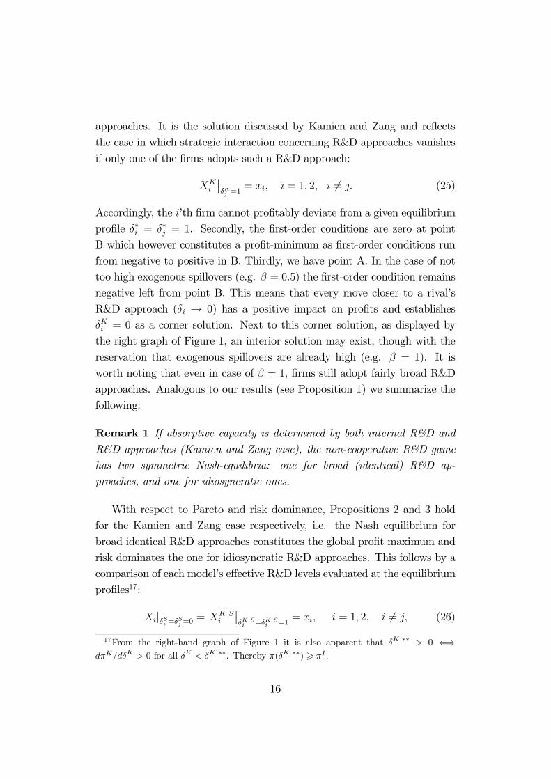
approaches. It is the solution discussed by Kamien and Zang and reflects
the case in which strategic interaction concerning R&D approaches vanishes
if only one of the firms adopts such a R&D approach:
XKi
¯δKj =1
= xi, i = 1, 2, i 6= j. (25)
Accordingly, the i’th firm cannot profitably deviate from a given equilibrium
profile δ∗i = δ∗j = 1. Secondly, the first-order conditions are zero at point
B which however constitutes a profit-minimum as first-order conditions run
from negative to positive in B. Thirdly, we have point A. In the case of not
too high exogenous spillovers (e.g. β = 0.5) the first-order condition remains
negative left from point B. This means that every move closer to a rival’s
R&D approach (δi → 0) has a positive impact on profits and establishes
δKi = 0 as a corner solution. Next to this corner solution, as displayed by
the right graph of Figure 1, an interior solution may exist, though with the
reservation that exogenous spillovers are already high (e.g. β = 1). It is
worth noting that even in case of β = 1, firms still adopt fairly broad R&D
approaches. Analogous to our results (see Proposition 1) we summarize the
following:
Remark 1 If absorptive capacity is determined by both internal R&D and
R&D approaches (Kamien and Zang case), the non-cooperative R&D game
has two symmetric Nash-equilibria: one for broad (identical) R&D ap-
proaches, and one for idiosyncratic ones.
With respect to Pareto and risk dominance, Propositions 2 and 3 hold
for the Kamien and Zang case respectively, i.e. the Nash equilibrium for
broad identical R&D approaches constitutes the global profit maximum and
risk dominates the one for idiosyncratic R&D approaches. This follows by a
comparison of each model’s effective R&D levels evaluated at the equilibrium
profiles17:
Xi|δSi =δSj =0 = XK Si
¯δK Si =δK S
i =1= xi, i = 1, 2, i 6= j, (26)
17From the right-hand graph of Figure 1 it is also apparent that δK ∗∗ > 0 ⇐⇒dπK/dδK > 0 for all δK < δK ∗∗. Thereby π(δK ∗∗) > πI .
16

Xi|δIi=δIj=1 = XK Ii
¯δK Ii =δK I
i =0= xi + βxj , i = 1, 2, i 6= j. (27)
Recall that model set-ups only differ in the firms’ effective R&D levelsXi and
XKi respectively. But by Remark 1, (26) and (27) this difference vanishes
endogenously through the firms’ choices of R&D approaches. In fact, by (27)
the DJ model set-up is obtained if we focus on the global profit maximum.
We can thus conclude
Remark 2 Based on Pareto and risk dominance both Kamien and Zang’sand our model predict that firms select broad (identical) R&D approaches.
In turn both models’ predictions concerning equilibrium R&D efforts, output
quantities and profits correspond to the predictions of the DJ model.
4 Conclusions
We find that competing firms tend to adopt identical R&D approaches to
achieve a high degree of connectedness which in turn reduces R&D appropri-
ability. This pattern is in accordance with anecdotal evidence, but has been
shown analytically only in the context of research joint ventures (i.e. joint
profit maximization). Next to direct gains (i.e. costless cost reductions) the
incentive to achieve low appropriability is due to a dilemma which otherwise
forces firms to invest aggressively in R&D.
The introduction of absorptive capacity in terms of R&D approaches is
unlikely to change the predictions of the DJ model. In fact it turns out that
both settings - the cooperative one (which was not the challenge here) and the
competitive one - ultimately lead to those identical broad R&D approaches
that imply the DJ formulation. Consequently, the DJ formulation of a firm’s
effective R&D level need not implicitly assume ”that the firms have formed
a research joint venture” as stated by Kamien and Zang (2000).
It is important to emphasize that our results are driven by the R&D ap-
proaches’ property of simultaneously affecting incoming and outgoing knowl-
edge flows. This explanation closes the gap between previous work that re-
ported information exchange between competitors (e.g. Baumol, 2000, Kultti
and Takalo, 1998) on the one hand, and those who found no such exchange
as an equilibrium strategy (e.g. Poyago-Theotoky, 1999, Kamien and Zang,
17

2000) on the other. With Kultti and Takalo (1998), we conclude that when-
ever firms find a device to assure the simultaneous sending and receiving
of information they will pursue this strategy, whereas they will not if they
face any risk of receiving less information in return (Poyago-Theotoky, 1999).
The application of absorptive capacity and R&D approaches is but the first
step to explain how even competing firms implicitly share their knowledge.
Apparently not only the incentive itself, but the way firms exchange informa-
tion is a promising field for future research. For instance, a framework that
incorporates trust in this context might be helpful to obtain new insights
(e.g. Bönte 2003).
Our analysis supplements recent findings by Anbarci et al. (2002). In
contrast to previous analyses (e.g. Kamien, Müller and Zang, 1992) they
point out that (exogenous) knowledge flows among competitors may improve
welfare as compared to perfectly appropriable R&D, provided that the degree
of complementarity in R&D outputs is sufficiently high. Yet the question of if
and how competing firms actually implement this mode of collaboration has
been left unresolved.18 Identical R&D approaches provide an interpretation
of how competing firms manage to foster knowledge flows between each other.
Acknowledgements The work in this paper was conducted in part while
the author was visiting the University of Notre Dame, whose hospitality is
gratefully acknowledged. I would like to thank Tom Gresik for helpful sug-
gestions and encouragement. This work gained significantly from discussions
with Werner Bönte, Stefan Napel and Wilhelm Pfähler. Thanks are also due
to Nina Carlsen, Heidrun Hoppe, Morton Kamien, Andrew Irving, Björn
Möller and participants at the European Summer School on Industrial Dy-
namics (ESSID 2003). I am grateful to an anonymous referee and Stephen
Martin, the editor, for their remarks. Errors and omissions are mine.
18Amir (2000) already explained the role of complementarity in R&D outputs by com-parison of the DJ and the KMZ framework.
18

Appendix
Proof of Proposition 1 First, suppose that β ∧ δi∧ δj 6= 0. Note that forδ∗∗i , i = 1, 2 constituting a Nash equilibrium it suffices to show that δ∗∗i is a
best response to δ∗∗j , i 6= j. As πi is continuously differentiable with respect
to δi,dπidδi
> 0 for all δi < δ∗∗i , i = 1, 2, i 6= j, (28)
implies δ∗∗i being a better response than any δi < δ∗∗i . The sign of the
derivative dπi/dδi can by (9) be computed as
sgndπidδi
= sgn2(−a+A)βδjΩi
3(Ψi)2, (29)
and thus dπi/dδi > 0⇔ Ωi < 0, where
Ωi = 16− 24βδiδj + 12(βδiδj)2 − 2(βδiδj)3 − 27γ + 27βδiδjγ. (30)
Next, define Ω0i := Ωi(γ = 8/9) and note that Ω0i < 0 ⇒ Ωi < 0 as by the
second-order condition γ > 8/9 and ∂Ωi/∂γ 6 0 for all β ∨ δi∨ δj 6 1. Thenwe have
Ω0i = 2(−4 + 6(βδiδj)2 − (βδiδj)3). (31)
Since ∂Ω0i/∂k > 0, k = β, δi, δj define Ω00i := Ω0i(β = 1, δj = δi = δ) and we
know that Ω00i < 0⇒ Ω0i < 0 as long as we look for simultaneously given bestresponses. The sign of dπi/dδi is thus determined by
Ω00i = 2(−4 + 6δ4 − δ6). (32)
Note thatΩ00i has a unique root for δ ≈ 0.94. In particular, Ω00i < 0⇔ δ < 0.94
and thereby δ < 0.94⇒ dπi/dδi > 0. This means that any symmetric Nashequilibrium in R&D approaches will satisfy δ∗∗ > 0.94. Moreover, existenceand uniqueness follows from (28) in the case of δ∗∗ = 1 and from (32) in thecase of δ∗∗ < 1 since dπi/dδi < 0 only if Ω00i > 0. We conclude by remarking
that given dπi/dδi changes its sign in δ∗∗ < 1 then dπi/dδi goes from positiveto negative and hence πi is maximized. This completes the proof of the first
claim.
19

The second claim follows immediately by similar arguments. In particu-
lar, define Ω000i := Ω0i(δj = δi = 1). Thus,
Ω000i = 2(−4 + 6β2 − β3). (33)
The unique root of Ω000i is β ≈ 0.884. Hence, β < 0.884 ⇒ dπi/dδi > 0 and
thereby establishes δ∗∗ = 1 being a corner solution. ¥
Proof of Lemma 1 By (2), (3) and (7) we can compute (subscripts are
omitted as we are interested in symmetric solutions)
sgn∂πI
∂β= sgn
16− 24β + 12β2 − 2β3 − 27γ + β27γ
(4 + 2β − 2β2 − 9γ)3 . (34)
Since γ > 8/9 by the second stage second-order condition, the denominator
of (34) is always negative. Note that the numerator of (34) is decreasing
in γ (for all β < 1) and for γ = 8/9 its unique root is β ≈ 0.884, (34)
being negative for β < 0.884. Thereby, ∂πI/∂β > 0, for all β < 0.884. The
term (−27γ + β27γ) indicates that the numerator tends to be negative for
β > 0.884 due to higher values of γ (γ > 8/9) whereby the uniqueness of the
root in β > 0.884 remains. Moreover, it is evident that the numerator of (34)
is certainly positive for β = 1. By continuity, this establishes the first and the
second claim of Lemma 1. The rest of the proof is straightforward following
arguments similar to those constituting δ∗ = 0 as a Nash equilibrium. In
particular, πSi /∂β = 0 because πSi itself cancels out any effects from β and
for β = 0, likewise any effects from differences in δ are cancelled out; hence
πSi¯β=0
= πSi¯β=0
. ¥
20

References
[1] Amir, R., (2000). Modelling imperfectly appropriable R&D via
spillovers. International Journal of Industrial Organization, 18, 1013-
1032.
[2] Anbarci, N., Lemke, R. and Santanu, R., (2002). Inter-firm complemen-
tarities in R&D: a re-examination of the relative performance of joint
ventures. International Journal of Industrial Organization, 20, 191-213.
[3] Baumol, W.J., (2001). When is inter-firm coordination beneficial? The
case of innovation. International Journal of Industrial Organization, 19,
727-737.
[4] Bönte, W., (2003). The Relevance of Knowledge Spillovers and Geo-
graphical Proximity for Trust in Buyer-Supplier Relations. Working Pa-
per, University of Hamburg.
[5] Cassiman, B., Perez-Castrillo, D. and Veugelers, R., (2002). Endogeniz-
ing know-how flows through the nature of R&D investments. Interna-
tional Journal of Industrial Organization, 20, 775-799.
[6] Cockburn, I., M. and Henderson, R., M., (1998). Absorptive capacity,
coauthoring behavior, and the organization of research in drug discovery.
Journal of Industrial Economics, 46, 157-182.
[7] Cohen, W.M. and Levinthal, D.A., (1989). Innovation and learning: The
two faces of R&D. The Economic Journal, 99, 569-596.
[8] D’Aspremont, C. and Jacquemin, A., (1988). Cooperative and Nonco-
operative R&D in Duopoly with Spillovers. American Economic Review,
78, 1133-1137.
[9] De Bondt, R., (1996). Spillovers and innovative activities. International
Journal of Industrial Organization, 15, 1-28.
[10] Grünfeld, L.A., (2003). Meet me halfway but don’t rush: absorptive
capacity and strategic R&D investment revisited. International Journal
of Industrial Organization, 21, 1091-1109.
21

[11] Hauenschild, N., (2003). On the role of input and output spillovers when
R&Dprojects are risky. International Journal of Industrial Organization,
21, 1065-1089.
[12] Kamien, M., Muller, E. and Zang, I., (1992). Research Joint Ventures
and R&D Cartels. The American Economic Review, 82, 1293-1306.
[13] Kamien, M and Zang, I., (2000). Meet me halfway: research joint ven-
tures and absorptive capacity, International Journal of Industrial Orga-
nization. 18, 995-1012.
[14] Kultti, K. and Takalo, T., (1998). R&D spillovers and information ex-
change. Economic Letters, 61, 121-123.
[15] Lim, K., (2000). The many faces of absorptive capacity: spillovers of
interconnect technology for semiconductor chips. MIT Sloan Working
Paper 4110.
[16] Martin, S., (2002). Spillovers, appropriability, and R&D. Journal of Eco-
nomics, 75, 1-32.
[17] Poyago-Theotoky, J.A., (1999). A Note on Endogenous Spillovers in a
Non-Tournament R&D Duopoly. Review of Industrial Organization, 15,
253-262.
[18] Schrader, S., (1990). Informal technology transfer between firms: Coop-
eration through information trading. Research Policy, 20, 153-170.
[19] Suzumura, K., (1992). Cooperative and Noncooperative R&D in an
Oligopoly with Spillovers. American Economic Review, 82, 1307-1320.
[20] von Hippel, E. (1987). Cooperation between rivals: Informal know-how
trading. Research Policy, 16, 291-302.
22

Cooperation or Competition in R&D
When Innovation and Absorption
Are Costly
Lars Wiethaus
January 2005, this version June 2005
Abstract
This paper analyses cost-reducing R&D investments by firms that
behave non-cooperatively or cooperatively. Firms face a trade-off be-
tween allocating their R&D investments to innovate or to imitate (ab-
sorb). We find that the non-cooperative behavior not only induces
more imitation (absorption) but also, for the most part, more inno-
vation investments. Only the cooperative behavior, however, ensures
that R&D investments are allocated efficiently to innovation and to
imitation (absorption) in the sense that any given amount of industry-
wide cost-reduction is obtained for the minimum overall R&D costs.
JEL Classification: O31, O32, L13Keywords: Absorptive Capacity, Cooperation; Spillovers; Innova-tion; Imitation; R&D.
1

1 Introduction
“European industry is investing too little in research and development
(R&D). Governments want to see Europe’s R&D investment rise from its
current 1.9% of GDP to 3% by 2010. And industry, they say, should pro-
vide most of that extra investment” (The Economist 2003, “Reinventing
Europe”). Yet to achieve this ambitious goal, policy makers might at least
want to provide appropriate investment incentives. Aimed at restoring firms’
incentives to engage in an activity whose results are only imperfectly appro-
priable due to knowledge spillovers, the European Commission has not only
relaxed competition law to allow cooperative R&D among competitors1 but
encourages the formation of research joint ventures (RJVs) explicitly. Se-
lected RJVs are receiving up to 50% of their costs whereby the Commission
estimated that more than 5000 RJVs were funded in the fourth Framework
Programme (1994-1998)2. Not surprisingly Caloghirou and Vonortas (2004)
report a considerable increase of RJVs in Europe since the mid 1980s. Hage-
doorn (2002) and Vonortas (1997) find the same pattern for worldwide and
for U.S. partnerships.
The increasing willingness to engage in cooperative R&D arguably reflects
some net benefit to the participating firms, arising, for instance, from R&D
cost and risk sharing, minimization of transaction costs and economies of
scale and scope3. Whether or not cooperative R&D does indeed stimulate
firms’ incentives to invest in R&D is far less definite and, by the same token,
increasing technological progress and consumers’ surplus are less clear cut.
1Barker and Cameron (2004) discuss block exemptions from Articles 81 and 82 of theEC Treaty (formerly Articles 85 and 86). U.S. policy moved in the same direction with the1984 enactment of the National Cooperative Research Act (NCRA) to allow cooperationin ’earlier’ stages of R&D. In 1993 the National Research and Production Act (NCRPA)extended cooperation to product development, prototyping and production (Geroski 1993,Vonortas 1997).
2The sixth Framework Programme (2002-2006) has a budget of 17.5 billion Euro, themost of which is devoted to RJV promotion, see Barker and Cameron (2004).
3Based on three categories of literature (i.e. transaction costs, strategic managementand industrial organization), Hagedoorn et al. (2000) provide an overview on theoreticalarguments related to incentives to form research partnerships and expected results fromresearch partnerships.
2

Seminal theoretical contributions4 by D’Aspremont and Jacquemin (1989)
and Kamien et. al. (1992) seem to confirm that cooperative R&D induces
more investments if knowledge spillovers are substantial: firms agree on high
R&D investments that maximize their joint profits instead of trying to free-
ride on each others’ efforts. Our analysis reveals that this R&D stimulating
effect of RJVs is significantly reduced (and may even vanish completely) if
one accounts for some specific costs of receiving spillovers.
Since the investment stimulating effect of cooperative R&D depends cru-
cially on the spillover-rate, previous recent theoretical studies by Kamien and
Zang (2000)5, Kaiser (2002 b), Grünfeld (2003), Martin (2003) and Leahy
and Neary (2004) have emphasized6 that knowledge spillovers, in turn, de-
pend on the firms’ ability to “identify, assimilate, and exploit knowledge from
the environment”, i.e. on the firms’ absorptive capacities as defined by Co-
hen and Levinthal (1989). These studies commonly incorporate the concept
of absorptive capacity by tying the receipt of spillovers to a firm’s own R&D.
This way, however, a firm receives valuable and applicable knowledge (i.e.
R&D or process-innovations) if and only if the firm itself creates valuable
and applicable knowledge for other firms to absorb.
Empirical evidence points in a different direction. Mansfield et al. (1981)
identify specific costs of imitation as “all costs of developing and introduc-
ing the imitative product, including applied research, product specification,
pilot plant or prototype construction, investment in plant and equipment,
and manufacturing and marketing start-up. (If there was a patent on the
innovation, the cost of inventing around it is included)”. On average these
costs represent up to 65% of the respective innovation cost. Link and Neufeld
(1986) find out that those who are in charge of R&D “employ different R&D
strategies, generally choosing between innovation or imitation” and Rosen-
berg and Steinmueller (1988) note that Japanese firms are very successful in
the absorption of American firms’ innovations whereas the Americans, “very
4See De Bondt (1996) for a survey. Kaiser (2002 a) provides an empirical study oncooperative and non-cooperative R&D in the German service sector.
5In contrast to Kamien and Zang’s prediction, Wiethaus (2005) demonstrates that non-cooperative firms tend to adopt identical R&D approaches, just like cooperative firms. Healso extends this finding to Kamien and Zang’s original model.
6Campisi et al. (2001) focus on the role of absorptive capacity in R&D competition.
3

good at innovation”, are rather poor imitators. Moreover Henderson and
Cockburn (1996) identify “costs of maintaining absorptive capacity, which
take the form here of large numbers of small and apparently unproductive
programs”. These observations suggest that a firm will imitate/absorb con-
tingent on specific costs rather than contingent on an own innovation.
The distinction between innovation and imitation/absorption alters previ-
ous results regarding the efficiency of non-cooperative and cooperative R&D
investment behavior and thus sheds some new light on the still prevalent
question: “to what extent R&D cooperation is preferred to R&D competi-
tion by both firms and societies [...]” (Sena 2004). With specific costs of
imitation/absorption cooperation only induces higher technological progress
and consumer surplus than the non-cooperative behavior if patent protection
is extremely weak and, at the same time, imitation/absorption is rather easy
from a technological point of view7. However, we also detect a new, welfare
enhancing, attribute of cooperative R&D investment decisions: resources tar-
geted to innovate on the one hand and those targeted to imitate/absorb on
the other are allocated efficiently in the sense that any given amount of cost
reduction is obtained for the minimum overall investment costs.
Kanniainen and Stenbacka (2000) also analyze the strategic interaction
between innovating and imitating firms. The authors focus, however, on the
implications of their results on subsidy and patent policy and do not address
how investment incentives are altered in the case of cooperation. The same
applies for Takalo’s (1998) model of innovation and imitation. Cassiman et
al. (2002) emphasize the role of investments in specific types of R&D such as
applied R&D, basic R&D and investments in intellectual property protection.
In contrast to our work their investigation is on non-cooperative investment
incentives of an incumbent firm facing a competitive fringe. Imitative and
7Based on the assumption that absorption requires no efforts at all, D’Aspremont andJaquemin (1989) found R&D cooperation to induce more efforts than R&D competition if50% of a firm’s R&D results spill over to its competitor in the product market. Accordingto Grünfeld (2003) this critical spillover rate shifts from 0.5 to about 0.618 due to the in-troduction of imitation/absorption as a function of innovation. With imitation/absorption
as a function of specific investments like in our model, cooperation might not at all inducehigher technological progress than the non-cooperative behaviour even if spillovers areperfect.
4

innovative R&D has, moreover, been analyzed by Hammerschmidt (1999) for
the non-cooperative case. If exogenous spillovers increase, imitative R&Dwill
increase whereas innovative R&D will decrease. On the one hand, we confirm
her results, though within a different model set-up (see below). On the other
hand, we extend her findings by the comparison of the non-cooperative case
with the cooperative one in terms of technological progress and allocative
efficiency of R&D investments.
The remainder of the paper is organized as follows. In section 2 we
introduce a two stage duopoly model. We describe how each firm’s first
stage investment in innovation and imitation/absorption translates into some
reductions of production costs. Then, for given amounts of cost reductions,
we derive the second stage Nash equilibrium in output quantities. Section 3
deals with the firms’ non-cooperative first-stage decisions. We formally (and
separately) analyze firms’ incentives to innovate and to imitate/absorb. This
yields intermediate results helping to explain intuitively the firms’ investment
behavior. The Nash equilibrium is described by numerical solutions. Section
4 proceeds in a similar fashion proposing, however, a cooperative solution
in the firms’ investment decisions. In section 5 we employ the results of
3 and 4 in order to establish the welfare implications of non-cooperative vs.
cooperative investment behavior in terms of technological progress, consumer
surplus and allocative efficiency of R&D investments. Section 6 concludes
and suggests directions for future research.
2 The Model
We consider a two-period duopoly model. In period 1, two identical firms i =
1, 2 determine their investment decisions aimed at process innovation. These
decisions are analyzed for both non-cooperative and cooperative behavior8.
In the second period firms compete in output-quantities, qi.
First period: investment in cost reductions Each firm can reduce
its constant marginal production costs, C, by a certain amount, Xi (cost
8We refer to the cooperative case if firms coordinate their decisions in order to maximizetheir joint profits, ceteris paribus.
5

reduction), through its efforts9 to generate a process-innovation, Ai, and its
efforts, Bi, to absorb/imitate the rival’s innovation, Aj.
We define innovation efforts, Ai, to include all activities that lower a firm’s
production costs through the creation and exploitation of new knowledge. In
turn innovation efforts not only benefit the ith firm but also enhances the
knowledge-pool potentially available for i’s rival j. Most obviously innovation
efforts contain some kind of applied R&D.
We define imitation/absorption efforts, Bi, to include all activities that
lower a firm’s production costs through the assimilation and exploitation of
externally created new knowledge (innovations). These efforts include im-
provements of a firm’s absorptive capacity in general (Cohen and Levinthal
1989) and all investments to implement the imitation in particular (Mans-
field et al. 1981). In turn innovation/absorption efforts do not per se provide
any new knowledge for another firm. Simply put the identification and as-
similation of new knowledge in form of a patent, its subsequent exploitation
in form of reverse-engineering and its application to commercial ends do cer-
tainly require R&D but do not require taking out a new patent or some
other sort of new knowledge. Also, instead of pushing R&D for one specific
application a firm may enhance its absorptive capacity by gaining a fuller
understanding of the broader scope of the research field. In this sense Rosen-
berg (1990) highlights the role of basic research “for evaluating the outcome
of much applied research and for perceiving its possible implications” and to
“understand, interpret and to appraise knowledge that has been placed upon
the shelf” (see Cassiman et al. 2003 for an application). A firm’s absorptive
capacity, moreover, “depends on the structure of communication between the
external environment and the organization, as well as among the subunits
of the organization [...]” (Cohen and Levinthal 1990). Obviously a firm can
establish and maintain a well-functioning organization in that sense without
benefiting its rival.
The ith firm’s cost reduction, Xi, can for example be written as the sum
of its own innovation efforts, Ai, and a Cobb-Douglas relationship10 between
9The terms efforts and investments are used synonymously throughout.10The Cobb-Douglas relationship is convenient for analytical tractability and because
parameters are easy to interpretate. Employing a CES function would be a more general
6

its efforts to imitate/absorb, Bi, and another firm’s innovation efforts, Aj,
Xi = Ai + βBαi A
1−αj , i = 1, 2, i 6= j. (1)
As we abstract from uncertainty, innovation efforts, Ai, correspond to in-
novation results. Imitation/absorption efforts, Bi, translate into imita-
tion/absorption results, βBαi A
1−αj , as a function of exogenous parameters
β, 0 6 β 6 1, and α, 0 6 α < 1 and, of course, Aj.
Note that higher values for α decrease the amount of cost reduction, Xi,
that the ith firm obtains for any given level of Bi 6 Aj (see Lemma 1),
whereas higher values for α (are likely to)11 reflect an increase the marginal
productivity of Bi. The economic interpretation of α is what Cohen and
Levinthal (1989) introduced as the difficulty of learning12. It is determined
by “the complexity of knowledge to be assimilated and the degree to which
the outside knowledge is targeted to the needs and concerns of the firm”.
Difficulty of learning makes imitation efforts, Bi, more critical to the ab-
sorption/imitation of a certain amount of Aj. Consequently α is likely to
increase the marginal productivity of Bi whereas it reduces i’s cost reduction
for given values of Aj and Bi, ceteris paribus. The counterpart expression,
(1− α), can be interpreted as the ease of learning, respectively.
A lower value of β, of course, reduces the amount of i’s cost reduction
for given values of Aj and Bi; in contrast to (a higher) α, however, a lower
β decreases the marginal productivity of Bi as well. The parameter β can
thus be interpreted as a measure of patent-protection. Stronger (weaker)
patent-protection, i.e. a lower (higher) β, decreases (increases) both the
approach, in particular, because it does not imply a substitution elasticicity of unitybetween Bi and Aj (I am grateful to an anonymeous referee who made this point). Howeverthis does not significantly alter the main qualitative results presented in section 5 (see alsofootnote 20). A robustness check is available from the author upon request.11If Bi is very small compared to Aj , an increase in α may, in fact, decrease the marginal
impact of Bi on Xi This is due to the model calibration with 0 6 α < 1.12Note that Cohen and Levinthal proposed that if learning became more difficult this
would always decrease the marginal impact of a firm’s own R&D on its absorptive capacity.This is in partial conflict, however, to the equal scale of innovation and imitation in (1)and thus in our model α does, for some parameter constellations not increase the marginalimpact of Bi on Xi.
7

level of another firm’s original innovation, Aj, that can be absorbed and the
marginal productivity of firm i’s efforts to absorb, Bi.
To clarify the difference between the legal dimension, β, and the techno-
logical dimension, α, consider the example of biotech drugs which are, despite
weak patent protection, difficult to copy as “the process is prone to conta-
mination and is highly variable, making the task complex and costly” (The
Economist 2003, “Carbon Copy”). Thus α is relatively high and β is rela-
tively low. Just the opposite seems to be true for conventional drugs where
patent protection is relatively strong but once patents expire, it becomes a
straightforward task to introduce a generic drug.
In line with the literature we propose that costs of innovation and imi-
tation/absorption are A2i and B2i respectively
13 which formalizes decreasing
returns to R&D investments.
Second period: Quantity competition In the product-market firms
compete in quantities with linear demand, P = a− bQ, where Q = qi + qj.
Initially firms have the same constant marginal production costs, Ci = Cj =
C. Thus, after innovation and imitation has occurred in the first period,
firms produce with constant marginal production costs C−Xi in the second
period. The ith firm’s profit-function can be expressed by
πi = (a− bQ)qi − (C −Xi)qi −A2i −B2i , i = 1, 2, i 6= j. (2)
The second stage Nash equilibrium is
q∗i = (a− C + 2Xi −Xj)/3b, i = 1, 2, i 6= j. (3)
Because variations in the parameters a, C and b do not change any of our
qualitative conclusions it is convenient to assume a − C = 1 and b = 1
throughout.
Focusing on the symmetric case the second-stage Nash equilibrium can
simply be expressed by
13An additional cost-parameter γ, as common in the literature, does not provide furtherinsights and since γ = 1 guarantees sufficiently concave profit-functions we can leave itout.
8

q∗ = (1 +X)/3 = (1 +A+ βBαA1−α)/3. (4)
Equation (4) reflects that in a symmetric equilibrium output quantities, q∗,and profits, π(q∗), are ceteris paribus increasing in weaker patent protection,β, and decreasing in the difficulty of learning, α, provided B < A (see Lemma
1). Of course, the higher β and the smaller α the stronger is knowledge
diffusion, ceteris paribus, and accordingly the larger is industry wide cost
reduction and market size. In the analyses to follow we will refer to q∗ as themarket size incentive to invest in R&D.
3 The non-cooperative investment case
Upon substitution of (3) into (2), the ith firm’s first-stage profit function can
be written as
π∗i = q∗i2 −A2i −B2
i , i = 1, 2, i 6= j, (5)
where the first-order conditions,
∂π∗i∂Ai
= q∗i∂q∗i∂Ai−Ai = 0, i = 1, 2, i 6= j, (6)
and∂π∗i∂Bi
= q∗i∂q∗i∂Bi−Bi = 0, i = 1, 2, i 6= j. (7)
have to be fullfilled simultaneously. Before we turn to the simultaneous
equilibrium we explore the incentives to innovate and the incentives to im-
itate/absorb separately. For the analyses to follow it is useful to have the
following intermediate result at hand:
Lemma 1 In the symmetric case any profit-maximizing simultaneous solu-tion to the first-order conditions (6) and (7) will satisfy B 6 A.
Proof. See appendix.
9
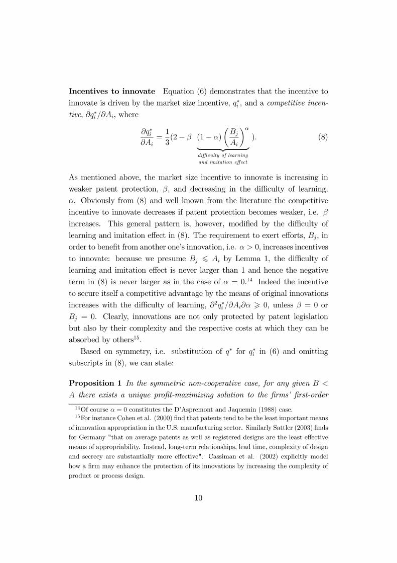
Incentives to innovate Equation (6) demonstrates that the incentive to
innovate is driven by the market size incentive, q∗i , and a competitive incen-tive, ∂q∗i /∂Ai, where
∂q∗i∂Ai
=1
3(2− β (1− α)
µBj
Ai
¶α
| z difficulty of learningand imitation effect
). (8)
As mentioned above, the market size incentive to innovate is increasing in
weaker patent protection, β, and decreasing in the difficulty of learning,
α. Obviously from (8) and well known from the literature the competitive
incentive to innovate decreases if patent protection becomes weaker, i.e. β
increases. This general pattern is, however, modified by the difficulty of
learning and imitation effect in (8). The requirement to exert efforts, Bj, in
order to benefit from another one’s innovation, i.e. α > 0, increases incentives
to innovate: because we presume Bj 6 Ai by Lemma 1, the difficulty of
learning and imitation effect is never larger than 1 and hence the negative
term in (8) is never larger as in the case of α = 0.14 Indeed the incentive
to secure itself a competitive advantage by the means of original innovations
increases with the difficulty of learning, ∂2q∗i /∂Ai∂α > 0, unless β = 0 or
Bj = 0. Clearly, innovations are not only protected by patent legislation
but also by their complexity and the respective costs at which they can be
absorbed by others15.
Based on symmetry, i.e. substitution of q∗ for q∗i in (6) and omittingsubscripts in (8), we can state:
Proposition 1 In the symmetric non-cooperative case, for any given B <
A there exists a unique profit-maximizing solution to the firms’ first-order
14Of course α = 0 constitutes the D’Aspremont and Jaquemin (1988) case.15For instance Cohen et al. (2000) find that patents tend to be the least important means
of innovation appropriation in the U.S. manufacturing sector. Similarly Sattler (2003) findsfor Germany "that on average patents as well as registered designs are the least effectivemeans of appropriability. Instead, long-term relationships, lead time, complexity of designand secrecy are substantially more effective". Cassiman et al. (2002) explicitly modelhow a firm may enhance the protection of its innovations by increasing the complexity ofproduct or process design.
10

conditions (6) in A. Denoting this solution A0 we have
sign∂A0
∂β= sign
à ∂q∗i∂Ai
¯i=j
!2− (1− α)
, (9)
and
sign∂A0
∂α= sign
à ∂q∗i∂Ai
¯i=j
!2− (1− α)
lnµBA
¶+ 1
. (10)
Proof. See appendix.Proposition 1 states how, for a given level of B, optimal innovation efforts
change if both the competitive incentive and the market size incentive are
taken into account. Equation (9) reveals that the sign of A0 in β depends
on the strengths of the (squared) competitive incentive relative to (1 − α),
the ease of learning. From (8) we can deduce that the squared competitive
incentive ranges between 1/9 and 4/9. Therefore if learning is easy, (1 −α) > 4/9, (9) is certainly negative. This is the commonly known case: the
decrease in the competitive incentive dominates the increase in the market
size incentive. However if learning is rather difficult, say (1 − α) < 4/9,
then efforts to innovate originally may increase in β which in turn implies
that the increase in the market size incentive dominates the decrease in the
competitive incentive16.
The sign of the derivative of A0 in α depends by (10) likewise on the
interplay between the squared competitive incentive and the ease of learning
(1−α). For the case that learning is rather easy, (1−α) > 4/9, we have just
established that the squared competitive incentive is certainly dominated.
Taking into account that ln(B/A) 6 0 we then have that (10) is positive.
Accordingly efforts to innovate increase if learning becomes more difficult.
This is due to the protection effect which increases the competitive incen-
tives. However if learning is already rather difficult and absorption/imitation
efforts B are low relative to A (that is ln(B/A) gets large), (10) is negative
16A more profound analysis of the causes and consequences of this result is beyond thescope of the present paper which aims to compare non-cooperative and cooperative R&Dinvestment incentives with each other. It shall be the subject to future research.
11

and if learning becomes more difficult this discourages innovation efforts.
Now the decrease in the market size incentive dominates the increase in the
competitive incentive.
Incentives to imitate/absorb By the first-order condition (7) the firms’
imitation efforts, Bi, are, analogous to the previous section, caused by the
market size incentive, q∗i , and the competitive incentive, ∂q∗i /∂Bi,
∂q∗i∂Bi
=2
3βα
µAj
Bi
¶1−α. (11)
The market size incentive to imitate/absorb is, once again by (4), increasing
in weaker patent protection, β, and decreasing in the difficulty of learning,
α. Alos taking the competitive incentive (11) into account reveals, not too
surprisingly, that efforts to imitate/absorb are unambiguously increasing if
patent protection becomes weaker. Moreover (11) confirms that the incentive
to imitate is increasing in the amount of “knowledge that has been placed
upon the shelf” (Rosenberg, 1990), Aj.
Proposition 2 In the symmetric non-cooperative case, for any given A >
B there exists a unique profit-maximizing solution to the firms’ first-order
conditions (7) in B. Denoting this solution B0 we have
∂B0
∂β> 0, (12)
and
sign∂B0
∂α= sign
12
Ã∂q∗i∂Bi
¯i=j
!2+ α
lnµBA
¶+ 1
. (13)
Proof. See appendix.Proposition 2 states the comparative statics of B, for a given level of
A, if both the market size and the competitive incentives are considered.
By (11) it is obvious that (13) is certainly positive if α is sufficiently small
whereas (13) is more likely to be negative the larger α and the larger the gap
between B and A. Of course, α > 0, initiates imitation/absorption incentives
in the first place. But also, if it gets too difficult to learn, high returns
12

of imitation/absorption investments in form of cheap external knowledge
diminish. By the same token (13) is more likely to be negative (positive) the
larger (smaller) Aj is relative to Bi.
Equilibrium characterization Since firms i = 1, 2 are identical we con-
sider a symmetric Nash equilibrium in Ai = Aj = A∗ and Bi = Bj = B∗
where A∗ and B∗ need to satisfy the first-order conditions (6) and (7) for thesymmetric case,
∂π∗i∂Ai
¯i=j
= q∗∂q∗i∂Ai
¯i=j
−A = 0 (14)
and∂π∗i∂Bi
¯i=j
= q∗∂q∗i∂Bi
¯i=j
−B = 0, (15)
in A and B simultaneously. Note that q∗ is given by (4) and derivatives(∂q∗i /∂Ai)|i=j and (∂q∗i /∂Bi)|i=j represent expressions (8) and (11) respec-tively omitting subscripts.
Unfortunately we cannot solve the first-order conditions (14) and (15) for
A∗ and B∗ explicitly. The parameter space, however, is limited by 0 6 β 6 1and 0 6 α < 1. Table 1 displays values for A∗ and B∗ as derived withMathematica for alternative parameter constellations17.
With one exception the results displayed in Table 1 suggest the following
regularities:
• Efforts to innovate, A∗, are decreasing (increasing) in β if α is small
(large). Moreover A∗ is increasing in the difficulty of learning, α.
• Efforts to imitate/absorb, B∗, are increasing in both β and α.
• The ratio of imitation/absorption efforts to innovation efforts, B∗/A∗,is increasing both in β and in α, whereby 0 6 B∗/A∗ 6 1.
The economic logic behind these results can be deduced from the effects as
discussed in the previous sections. Intuitively appealing imitation/absorption
17The results displayed in Table 1 remain robust with respect to alternative starting
values for the numerical solution procedure.
13

α β
0 0.2 0.5 0.8 1.0
0
B∗/A∗
B∗
A∗
0
0
2.857
0
0
2.631
0
0
2.222
0
0
1.754
0
0
1.429
0.2
B∗/A∗
B∗
A∗
0
0
2.857
0.173
0.476
2.757
0.306
0.775
2.532
0.430
0.958
2.223
0.520
1.028
1.978
0.5
B∗/A∗
B∗
A∗
0
0
2.857
0.219
0.622
2.846
0.420
1.118
2.799
0.608
1.639
2.700
0.740
1.912
2.582
0.8
B∗/A∗
B∗
A∗
0
0
2.857
0.218
0.629
2.884
0.477
1.423
2.984
0.727
2.228
3.147
0.9
2.963
3.293
0.99
B∗/A∗
B∗
A∗
0
0
2.857
0.201
0.582
2.890
0.499
1.534
3.073
0.796
2.770
3.477
0.995
3.937
3.957B∗ : equilibrium imitation/absorption efforts (times 10)
A∗ : equilibrium innovation efforts (times 10)
Table 1: Innovation and imitation/absorption efforts in the non-cooperative
equilibrium
efforts are increasing if patent protection decreases. By the same token ef-
forts to innovate decrease in β because the potential competitive advantage
diminishes if one’s rival gets in possession of the innovation as well. This is
true, however, if and only if learning is rather easy (small α). Otherwise, if
learning is sufficiently difficult and imitation/absorption costly respectively,
competitive advantages from innovation tend to persist. Along with increas-
ing market size incentives, then, even efforts to innovate increase in β.
Generally an increase in the difficulty of learning, α, increases both in-
novation efforts and imitation/absorption efforts. The former is due to the
technical protection of innovations whereas the latter stems from the fact
that difficulty of learning renders imitation/absorption efforts more produc-
14
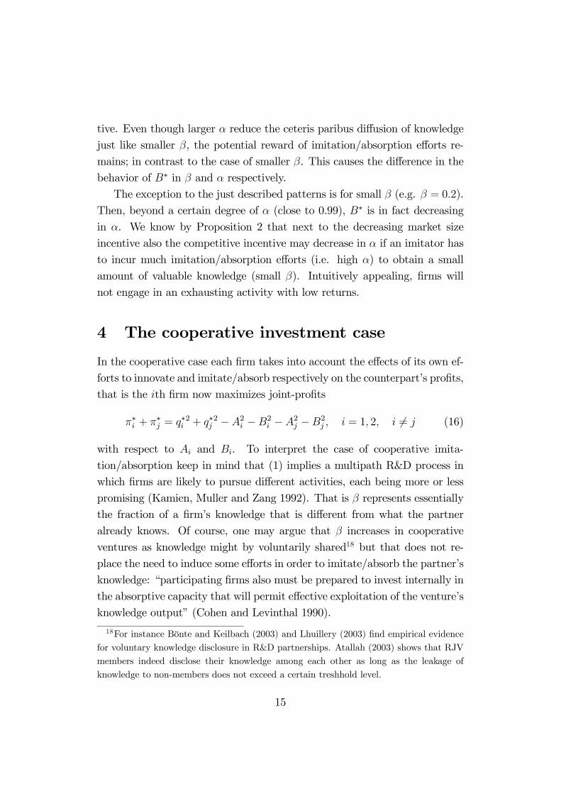
tive. Even though larger α reduce the ceteris paribus diffusion of knowledge
just like smaller β, the potential reward of imitation/absorption efforts re-
mains; in contrast to the case of smaller β. This causes the difference in the
behavior of B∗ in β and α respectively.
The exception to the just described patterns is for small β (e.g. β = 0.2).
Then, beyond a certain degree of α (close to 0.99), B∗ is in fact decreasingin α. We know by Proposition 2 that next to the decreasing market size
incentive also the competitive incentive may decrease in α if an imitator has
to incur much imitation/absorption efforts (i.e. high α) to obtain a small
amount of valuable knowledge (small β). Intuitively appealing, firms will
not engage in an exhausting activity with low returns.
4 The cooperative investment case
In the cooperative case each firm takes into account the effects of its own ef-
forts to innovate and imitate/absorb respectively on the counterpart’s profits,
that is the ith firm now maximizes joint-profits
π∗i + π∗j = q∗i2 + q∗j
2 −A2i −B2i −A2j −B2
j , i = 1, 2, i 6= j (16)
with respect to Ai and Bi. To interpret the case of cooperative imita-
tion/absorption keep in mind that (1) implies a multipath R&D process in
which firms are likely to pursue different activities, each being more or less
promising (Kamien, Muller and Zang 1992). That is β represents essentially
the fraction of a firm’s knowledge that is different from what the partner
already knows. Of course, one may argue that β increases in cooperative
ventures as knowledge might by voluntarily shared18 but that does not re-
place the need to induce some efforts in order to imitate/absorb the partner’s
knowledge: “participating firms also must be prepared to invest internally in
the absorptive capacity that will permit effective exploitation of the venture’s
knowledge output” (Cohen and Levinthal 1990).
18For instance Bönte and Keilbach (2003) and Lhuillery (2003) find empirical evidencefor voluntary knowledge disclosure in R&D partnerships. Atallah (2003) shows that RJVmembers indeed disclose their knowledge among each other as long as the leakage ofknowledge to non-members does not exceed a certain treshhold level.
15

The cooperative first-order conditions for each firm are given by
∂(π∗i + π∗j)∂Ai
= q∗i∂q∗i∂Ai
+ q∗j∂q∗j∂Ai−Ai = 0, i = 1, 2, i 6= j (17)
and∂(π∗i + π∗j)
∂Bi= q∗i
∂q∗i∂Bi
+ q∗j∂q∗j∂Bi−Bi = 0, i = 1, 2, i 6= j. (18)
In the following two sections we analyze the effects of cooperation on the
incentives to innovate and on the incentives to imitate/absorb separately.
Then we turn to the comparison of the simultaneous cooperative and non-
cooperative equilibrium. Similar to the non-cooperative case we can state:
Lemma 2 In the symmetric cooperative case any profit-maximizing simulta-neous solution to the first-order conditions (17) and (18) will satisfy B 6 A.
Proof. See appendix.
Effects of cooperation on incentives to innovate Comparing the non-
cooperative first-order condition (6) with the cooperative one (17), reveals
that the sign of∂q∗j∂Ai
=1
3(2β (1− α)
µBj
Ai
¶α
| z difficulty of learningand imitation effect
− 1), (19)
determines whether the non-cooperative or the cooperative mode induces
stronger efforts to innovate. As long as a firm’s innovation efforts increase a
rival’s equilibrium output quantity and (19) is positive, the cooperative mode
encourages by (17) innovation efforts as compared to the non-cooperative
mode, (6), and vice versa.
How is the sign of (19) shaped in the light of the difficulty of learning and
imitation effect? If there is no need to learn at all (i.e. α = 0) the labeled
part of (19) vanishes and the treshhold level β ≶ 0.5 of the D’Aspremont
and Jacquemin (1989) model alone determines which of the two cases induces
stronger incentives to innovate. However, if efforts to imitate/absorb become
more important the derivative (∂q∗j/∂Ai) decreases, i.e.
∂2q∗j∂Ai∂α
= −23β
µBj
Ai
¶αµ1− (1− α) ln
µBj
Ai
¶¶6 0. (20)
16

The sign follows because Bj 6 Ai and hence the second bracketed term in
(20) is non-negative. Thereby the higher α the more likely (19) is negative
and the more likely does the non-cooperative mode induce stronger incentives
to innovate as compared to the cooperative one.
On the other hand (19) is increasing in both weaker patent protection,
β, and another firm’s efforts to absorb, Bj. Either effect fosters knowledge
flows and thereby reduces the possibility to gain a competitive advantage in
the quantity competition (second-stage).
Effects of cooperation on incentives to imitate/absorb The effect of
imitation efforts, Bi, on a rival’s equilibrium output-quantity, q∗j ,
∂q∗j∂Bi
= −13βα
µAj
Bi
¶1−α, (21)
is non-positive which means by (18) and (7) that firms reduce efforts to
imitate/absorb in the cooperative case relative to the non-cooperative case.
Imitation/absorption reduces the imitator’s costs but, unlike innovation, does
not provide a direct positive externality that might create additional invest-
ment incentives if firms cooperate. In contrast, upon intensified product-
market competition, imitation/absorption indirectly hurts the counterpart’s
profits. Cooperation allows firms to internalize this negative externality and
accordingly softens the intensity of product-market competition .
Equilibrium characterization The first-order conditions for a joint profit
maximum in the symmetric cooperative case is obtained upon substitution
of (8) and (19) into (17) and respectively of (11) and (21) into (18):
∂(π∗i + π∗j)∂Ai
¯i=j
= q∗∂q∗i∂Ai
¯i=j
+ q∗∂q∗j∂Ai
¯i=j
−A = 0, (22)
and∂(π∗i + π∗j)
∂Bi
¯i=j
= q∗∂q∗i∂Bi
¯i=j
+ q∗∂q∗j∂Bi
¯i=j
−B = 0. (23)
Proceeding in a similar fashion as in the non-cooperative case we obtain
numerical solutions to (22) and (23) in A and B for alternative parameter
values of β and α. Denoting these solutions A and B, Table 2 provides some
17
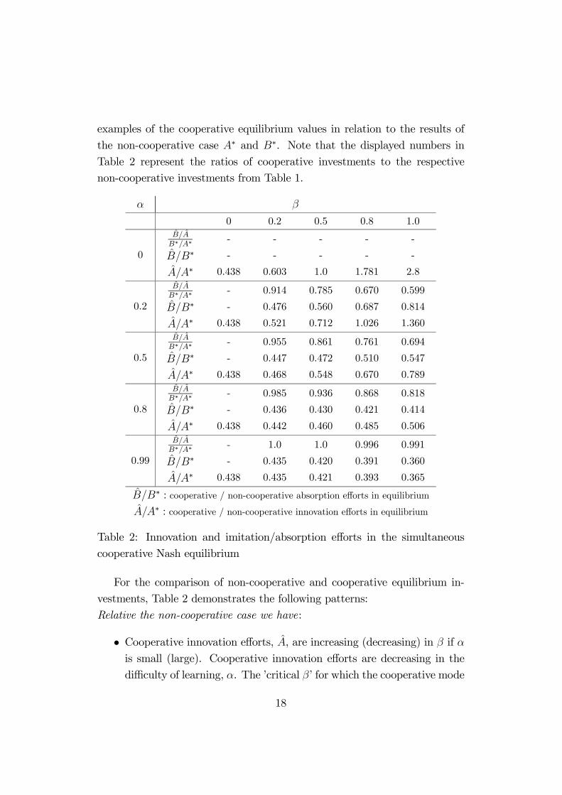
examples of the cooperative equilibrium values in relation to the results of
the non-cooperative case A∗ and B∗. Note that the displayed numbers inTable 2 represent the ratios of cooperative investments to the respective
non-cooperative investments from Table 1.
α β
0 0.2 0.5 0.8 1.0
0
B/AB∗/A∗
B/B∗
A/A∗
-
-
0.438
-
-
0.603
-
-
1.0
-
-
1.781
-
-
2.8
0.2
B/AB∗/A∗
B/B∗
A/A∗
-
-
0.438
0.914
0.476
0.521
0.785
0.560
0.712
0.670
0.687
1.026
0.599
0.814
1.360
0.5
B/AB∗/A∗
B/B∗
A/A∗
-
-
0.438
0.955
0.447
0.468
0.861
0.472
0.548
0.761
0.510
0.670
0.694
0.547
0.789
0.8
B/AB∗/A∗
B/B∗
A/A∗
-
-
0.438
0.985
0.436
0.442
0.936
0.430
0.460
0.868
0.421
0.485
0.818
0.414
0.506
0.99
B/AB∗/A∗
B/B∗
A/A∗
-
-
0.438
1.0
0.435
0.435
1.0
0.420
0.421
0.996
0.391
0.393
0.991
0.360
0.365
B/B∗ : cooperative / non-cooperative absorption efforts in equilibriumA/A∗ : cooperative / non-cooperative innovation efforts in equilibrium
Table 2: Innovation and imitation/absorption efforts in the simultaneous
cooperative Nash equilibrium
For the comparison of non-cooperative and cooperative equilibrium in-
vestments, Table 2 demonstrates the following patterns:
Relative the non-cooperative case we have:
• Cooperative innovation efforts, A, are increasing (decreasing) in β if α
is small (large). Cooperative innovation efforts are decreasing in the
difficulty of learning, α. The ’critical β’ for which the cooperative mode
18

induces higher investments than the non-cooperative one, A > A∗, isincreasing in the difficulty of learning, α.
• Cooperative efforts to imitate/absorb, B, are, similar to A, increas-
ing (decreasing) in β if α is small (large). Cooperative efforts to im-
itate/absorb, B, are decreasing in α. Within the complete parame-
ter range, cooperative efforts to imitate/absorb are lower than non-
cooperative ones.
• In the cooperative mode firms allocate less recourses to imitate/absorb.This divergence is increasing both in β and in α.
The results of Table 2 reveal that the R&D stimulating feature of co-
operation hinges rather critically on the presumption that no specific imi-
tation/absorption efforts are needed on the beneficiary’s side. For instance
α = 0.2 is sufficient to shift the well known β = 0.5 treshhold19 roughly up
to β = 0.8 and if α = 0.5 the non-cooperative mode unambiguously creates
stronger incentives to innovate than the cooperative one (e.g. A/A∗ = 0.630for β = 1). With regard to industry-wide cost reductions (i.e. technological
progress) and consumer surplus, however, the combined effect of innovation
and imitation/absorption efforts in equilibrium have to be considered. The
next section deals with this question and determines the critical values for β
and α at which the cooperative mode yields higher technological progress.
5 Welfare
Technological progress and consumer surplus Consumer surplus is
measured by the output quantities produced in (the symmetric) equilibrium
(4), whereX has to be substituted by the technological progress (i.e. effective
cost reduction) which is attained in the non-cooperative equilibrium
X∗ = A∗ + βB∗α
A∗1−α
,
19This is the critical spillover-level in the D’Aspremont and Jacquemin (1989) model, upto which cooperative efforts are higher than non-cooperative ones (see first line of Table2). Halmenschlager (2004) finds a critical spillover-level of 1/3 if two lagging firms conductR&D in order to catch up with one leader.
19

and the cooperative equilibrium respectively,
X = A+ βBα
A1−α
.
It is obvious that
X∗ − X ≶ 0⇐⇒ q∗(X∗) ≶ q∗(X).
As we cannot provide an explicit analytical solution for A∗, B∗ and A, B we
can neither do so for X∗ and X.
Nonetheless we offer a numerical approximation. In particular we sub-
stitute all the equilibrium solutions for (A∗, B∗) and (A, B), which from a
few were presented in Tables 1 and 2, into X∗ and X respectively. We then
obtain a list of numerical values for X∗ − X as a function of α and β. The
line in Figure 1 depicts all combinations of α and β at which X∗ − X = 0.
Figure 1 is a contour plot20 of the values we obtained for X∗ − X, that is a
geographic map of X∗ − X at which each contour joins values of the same
height. We modified the plot such that only the null contour was actually
plotted. To the north-west of the line X∗ − X > 0 and to the south-east
we have that X∗ − X < 0. Thus for a broad range of parameter constel-
lations, technological progress and consumer surplus is indeed lower in the
cooperative case as compared to the non-cooperative one21.
What restores non-cooperative incentives and respectively destroys coop-
erative incentives so fundamentally? One can think of two major effects that
increase non-cooperative investment incentives rather than cooperative ones.
First the requirement to exert specific costs in order to imitate/absorb pro-
tects innovations. Thereby firms profit more effectively from innovating in
the non-cooperative case because they can achieve a competitive advantage
rather exclusively (see (8)) whereas the positive externalities to be shared for
20In fact Figure 1 is a ListContourPlot of X∗ − bX. The Mathematica file is availablefrom the author upon request.21A robustness-check of these results, employing a CES function instead of the Cobb-
Douglas form in (1), is available from the author upon request. For reasonable parameter-extensions our results become more pronounced in the sense that the region of X∗ < bXdecreases. In addition, the mathematica file underlying Figure 1 (and intermediate resultsof the paper) is available upon request.
20

0.25 0.5 0.75 1
0.10.20.30.40.50.60.70.80.9
10.25 0.5 0.75 1
0.10.20.30.40.50.60.70.80.91
β
α
* ˆX X>
* ˆX X<0.25 0.5 0.75 1
0.10.20.30.40.50.60.70.80.9
10.25 0.5 0.75 1
0.10.20.30.40.50.60.70.80.91
β
α
* ˆX X>
* ˆX X<
Figure 1: Parameter constellations of α and β that determine whether
the non-cooperative case, or the cooperative case yields larger technologi-
cal progress, X∗, bX, and consumer surplus, q∗(X∗), q∗( bX).free in the cooperative case diminish by (19). The second reason stems from
the fact that the alternative way to obtain a cost reduction, namely through
imitation/absorption, does from another firm’s point of view not at all pro-
vide any positive externality but only intensifies competition in the product
market (see (11) vs. (21)). Hence, in this case cooperation only serves as a
device to cut back on aggressive investments to imitate/absorb which hurts
technological progress and consumers relative to the non-cooperative case.
Allocative efficiency of R&D investments In the non-cooperative case
firms always allocate a larger fraction of their overall investments to imi-
tate/absorb as compared to the cooperative case. This raises the question
which case induces the more efficient allocation in the sense that a given level
of cost reduction, Xi, is attained for minimum overall investments. We de-
rive the non-cooperative and the cooperative equilibrium allocation of efforts,
B∗/A∗ and B/A, and then compare these with the efficient allocation.
As for the non-cooperative and the cooperative case we have by (14) and
(15) and respectively (22) and (23):
21

Proposition 3 In equilibrium firms allocate their efforts in the ratio that
equals the ratio of the competitive incentives, i.e.
in the non-cooperative case
B∗
A∗=
∂q∗i∂Bi
¯A∗, B∗
∂q∗i∂Ai
¯A∗, B∗
=2βα
¡A∗B∗¢1−α
2− β(1− α)¡B∗A∗¢α , (24)
and in the cooperative case
B
A=
³∂q∗i∂Bi
+∂q∗j∂Bi
´¯A,B³
∂q∗i∂Ai
+∂q∗j∂Ai
´¯A,B
=βα³AB
´1−α1 + β(1− α)
³BA
´α . (25)
Proof. Substitution of (15) into (14) via q∗ implies (24) and substitutionof (23) into (22) via q∗ implies (25).Next, if firms allocate their R&D resources efficiently, each investment-
type, Ai and Bi, is employed such that the marginal overall cost reduction
due to the investment, ∂(Xiqi +Xjqj)/∂Ai and ∂(Xiqi +Xjqj)/∂Bi, equals
the marginal cost of the respective investment-type, 2Ai and 2Bi:
∂(Xiq∗i +Xjq
∗j )
∂Ai
¯i=j
= (q∗ +X
3)
µ1 + β(1− α)
µB
A
¶α¶= 2A (26)
and∂(Xiq
∗i +Xjq
∗j )
∂Bi
¯i=j
= (q∗ +X
3)
Ãβα
µA
B
¶1−α!= 2B (27)
In any case where (26) and (27) are not satisfied simultaneously it is possible
to achieve a higher cost reduction (or technological progress) for given R&D
costs through re-allocation of Ai and Bi. This brings us to
Proposition 4 In the efficient case firms allocate their resources in the sameratio as in the cooperative case, i.e.
B
A=
βα¡AB
¢1−α1 + β(1− α)
¡BA
¢α . (28)
22

Proof. We substitute (27) into (26) via (q∗+X/3) and solve for B/A to
get (28). Comparison of (28) and (25) completes the proof.
To understand the logic behind Proposition 4 one may view cooperation
as to comprise two independent optimization procedures: first on the overall
investment level and, secondly, on the allocation of this investment level ei-
ther to innovate or to imitate/absorb. Obviously, once the investment level
is fixed, it is certainly Pareto optimal from the firms’ point of view to allo-
cate efforts such that overall cost reductions, Xiq∗i + Xjq
∗j , are maximized.
The divergence between the non-cooperative allocation to the optimal (co-
operative) allocation is displayed by the ratio (B/A)/(B∗/A∗) in Table 2:the misallocation of R&D resources gets more pronounced the weaker patent
protection, β, and the larger the ease of learning, (1− α).
6 Conclusions
This paper has analyzed how the introduction of specific imitation and ab-
sorption efforts affects non-cooperative and cooperative incentives to invest in
cost reductions. Two main findings are contributed. First, non-cooperative
incentives to invest in cost-reducing R&D (whether for imitative/absorptive
or for innovative purposes) are, for the most part, larger than cooperative
ones. Second, only in the cooperative case, however, firms will allocate their
resources efficiently in the sense that the maximum industry-wide cost re-
duction is obtained for any given level of overall investments. The non-
cooperative case, in contrast, induces too much imitation/absorption relative
to innovation. Simply put, cooperation (RJVs) might be rather ineffective in
creating incentives whereas it guarantees that resources are not wasted. We
conclude that cooperation is hardly beneficial from the consumers’ point of
view, inducing, for the most part, less technological progress and consumer
surplus than the non-cooperative case whereas from the firms’ perspective
cooperation appears even more attractive than previously assumed.
European governments have clearly stated their primary goal of R&D
policy, namely to rise R&D investments up to 3% of GDP by 2010. Our
results suggest that the relaxation of competition law combined with sub-
stantial funding of cooperative R&D might not always be the appropriate
23

tool to induce increasing R&D investments when it comes to horizontally
related firms. While there may exist other good reasons to encourage coop-
erative R&D among product-market competitors, weak R&D appropriability
is hardly a sufficient condition if one agrees that receipt of spillovers requires
some, if moderate, specific investments.
A profound theoretical welfare analysis, of course, has to trade-off the
negative consumers’ perspective and the positive firms’ perspective against
each other. Future theoretical work should investigate under which circum-
stances the loss of technological progress might be outweighed by the increase
in the firms’ profits and an efficient allocation of R&D resources. Moreover
it would be interesting to know empirically whether there exist industry pat-
terns regarding the difficulty of learning.
Acknowledgements I am very grateful to Werner Bönte, Stefan
Napel, Tom Gresik and Wilhelm Pfähler for helpful comments. Thanks are
also due to Johannes Bruder, Ludwig Burger, Nina Carlsen and Stephan
Tolksdorf. Three anonymous referees provided very helpful comments. Spe-
cial thanks go to Stéphane Lemarie for a thorough discussion of the paper at
the conference Industrial Organization and Innovation 2005 in Grenoble.
24

Appendix
Proof of Lemma 1 and Propositions 1 and 2. For notational conve-
nience let
FA = q∗fqA −A = 0, (29)
and
FB = q∗fqB −B = 0 (30)
denote the first-order conditions (14) and (15) respectively where
fqA =∂q∗i∂Ai
¯i=j
=1
3
µ2− β(1− α)
µB
A
¶α¶, (31)
and
fqB =∂q∗i∂Bi
¯i=j
=2
3βα
µA
B
¶1−α. (32)
Lemma 1. We proceed by showing that the left hand side of (30) is
non-positive if (29) is satisfied and B = A. Then the fact that ∂FB/∂B < 0
if B > A completes the proof.
Upon substitution of A for B in (30) we have
FB|B=A =2
9βα(1 +A(β + 1))−A, (33)
whereas upon substitution of A for B, (29) can be solved for
A =2− β(1− α)
1− (β + 1)(2− β(1− α)). (34)
Then we substitute (34) into (33) to obtain
FB| B=A|FA=0 = −2− β − βα
7− β(1− α) + β2(1− α)6 0. (35)
Next∂FB
∂B
¯B>A
=∂q∗
∂BfqB + q∗
∂fqB∂B− 1 < 0, (36)
follows because
∂q∗
∂BfqB
¯B>A
=2
9
Ãβα
µA
B
¶1−α!26 2
9(37)
25

and ∂fqB/∂B 6 0 by (32). Thus the first-order condition (30) is non-positiveif B = A and if B > A it must be smaller. But then FB cannot go from
positive to negative in B if both B > A and (29) is satisfied. ¥
Proposition 1. By the implicit function rule, if
∂FA
∂A=
∂q∗
∂AfqA + q∗
∂fqA∂A− 1 6= 0 (38)
there exists a function A0 = f(B, β, α) that satisfies (29) in A and has partial
derivatives∂A0
∂β= −∂FA/∂β
∂FA/∂A(39)
and∂A0
∂α= −∂FA/∂α
∂FA/∂A. (40)
In order to evaluate (38) note that for the first term we have
∂q∗
∂AfqA 6
4
9(41)
because∂q∗
∂A=1
3
µ1 + β(1− α)
µB
A
¶α¶6 2
3(42)
and fqA 6 2/3 by (31). In order to evaluate the second term we substitute
the solution to (29) via q∗ = A/fqA into (38) and re-write the second term
asA
fqA
∂fqA∂A
=βα(1− α)Bα
2Aα − β(1− α)Bα6 3− 2
√2. (43)
Then by (41) and (43), (38) is strictly negative and A0 exists.Moreover, since
FA|A=0 = 2/9 > 0 (44)
the function A0 establishes the values for A in which (29) goes from positiveto negative and thus establishes a profit-maximum. (First claim).
Next, since ∂FA/∂A < 0 we have by (39) that
sign∂A0
∂β= sign
∂FA
∂β(45)
26

where∂FA
∂β=
∂q∗
∂βfqA + q∗
∂fqA∂β
(46)
Substituting the solution to (29) into (46) via q∗ = A/fqA yields
∂FA
∂β
¯FA=0
= BαA1−α(fqA)
2 − (1− α)
fqA. (47)
Since the denominator of (47) is strictly positive we have
sign∂A0
∂β= sign
£(fqA)
2 − (1− α)¤. (48)
This establishes the second claim.
Finally, be similar arguments we have
sign∂A0
∂α= sign
∂FA
∂α(49)
where∂FA
∂α=
∂q∗
∂αfqA + q∗
∂fqA∂α
. (50)
Again we substitute the solution to (29) into (50) via q∗ = A/fqA and obtain
∂FA
∂α
¯FA=0
= βBαA1−α((fqA)
2 − (1− α)) ln¡BA
¢+ 1
fqA. (51)
Hence
sign∂A0
∂α= sign
·((fqA)
2 − (1− α)) ln
µB
A
¶+ 1
¸(52)
This establishes the third claim.¥
Proposition 2. By the implicit function rule, if
∂FB
∂B=
∂q∗
∂BfqB + q∗
∂fqB∂B− 1 6= 0 (53)
the function B0 = f(A, β, α) that satisfies (30) in B exists and has partial
derivatives∂B0
∂β= − ∂FB/∂β
∂FB/∂B(54)
and∂B0
∂α= − ∂FB/∂α
∂FB/∂B. (55)
27

Upon substitution of (30) via fqB = B/q∗ into (53) we know that
∂q∗
∂BfqB
¯FB=0
=∂q∗
∂B
B
q∗=
βαBαA1−α
1 +A+ βBαA1−α< 1 (56)
whereas ∂fqB/∂B 6 0 and thus (53) is strictly negative.Moreover,
FB|B=0 =∞ (57)
and thereby the function B0 establishes the values for B in which (30) goes
from positive to negative and thus constitutes a profit-maximum. (First
claim).
Obviously ∂B0/∂β > 0 as both ∂q∗/∂β > 0 and ∂fqB/∂β > 0. (Second
claim).
Finally, applying the implicit-function-rule again, since ∂FB/∂B < 0 we have
sign∂B0
∂α= sign
∂FB
∂α(58)
where∂FB
∂α=
∂q∗
∂αfqB + q∗
∂fqB∂α
. (59)
Substitution of q∗ = B/fqB as implied by (30) yields
∂FB
∂α=1
3ln
B
AβBαA1−αfqB +
B
α
µ1− α ln
A
B
¶, (60)
which, after some re-arrangements, implies
sign∂B0
∂α= sign
·1 + ln
B
A
µ1
2(fqB)
2 + α
¶¸. (61)
¥
Proof of Lemma 2. For notational convenience let
CA = q∗cqA −A = 0 (62)
and
CB = q∗cqB −B = 0 (63)
28

denote the cooperative first-order conditions (22) and (23) respectively where
cqA =∂q∗i∂Ai
¯i=j
+∂q∗j∂Ai
¯i=j
=1
3
µ1 + β(1− α)
µB
A
¶α¶, (64)
and
cqB =∂q∗i∂Bi
¯i=j
+∂q∗j∂Bi
¯i=j
=1
3βα
µA
B
¶1−α. (65)
The proof of Lemma 2 follows by similar arguments as the proof of Lemma
1. We have
CB| B=A|CA=0 = −1− β(2α− 1)
8− β(2− α)− β2(1− α)6 0. (66)
Moreover∂CB
∂B
¯B>A
=∂q∗
∂BcqB + q∗
∂cqB∂B− 1 < 0, (67)
follows because
∂q∗
∂BcqB
¯B>A
=
Ã1
3βα
µA
B
¶1−α!26 1
9(68)
and ∂cqB/∂B 6 0 by (65). ¥
29

References
[1] Atallah, A. (2003). Information Sharing and the Stability of Cooper-
ation in Research Joint Ventures. Economics of Innovation and New
Technology, 12, 531-554.
[2] Barker, K., Cameron, H. (2004). European Union science and technol-
ogy policy, RJV collaboration and competition policy. In: Caloghirou,
Y., Vonortas, N.S., Ioannides, S. (Eds.). European Collaboration in Re-
search and Development. Cheltenham, UK, Edward Elgar.
[3] Bönte, W., Keilbach, M. (2005). Concubinage or Marriage? Informal
and Formal Cooperations for Innovation. International Journal of In-
dustrial Organization, 23, 279-302.
[4] Campisi, D., Mancuso, P., Nastasi, A. (2001). R&D Competition, Ab-
sorptive Capacity and Market Shares. Journal of Economics, 73, 57-80.
[5] Cassiman, B., Perez-Castrillo, D., Veugelers, R. (2002). Endogenizing
know-how flows through the nature of R&D investments. International
Journal of Industrial Organization, 20, 775-799.
[6] Cassiman, B., Veugelers (2002). Complementarity in the Innovation
Strategy: Internal R&D, External Technology Acquisition, and Cooper-
ation in R&D. Working Paper, EARIE 2002.
[7] Cohen, W.M., Levinthal, D.A. (1989). Innovation and learning: The two
faces of R&D. The Economic Journal, 99, 569-596.
[8] Cohen, W.M., Levinthal, D.A. (1990). Absorptive Capacity: A New Per-
spective on Learning and Innovation. Administrative Science Quarterly,
35, 128-152.
[9] Cohen, W.M., Nelson, R.R., Walsh, J.P. (2000). Protecting their Intel-
lectual Assets: Appropriability Conditions and why U.S. Manufacturing
Firms Patent (or not). NBER Working Paper 7552.
30

[10] Caloghirou, Y., Vonortas, N.S. (2004). RJVs in Europe: trends, per-
formance, impacts. In: Caloghirou, Y., Vonortas, N.S., Ioannides, S.
(Eds.). European Collaboration in Research and Development. Chel-
tenham, UK, Edward Elgar.
[11] D’Aspremont, C., Jacquemin, A. (1988). Cooperative and Noncoopera-
tive R&D in Duopoly with Spillovers. American Economic Review, 78,
1133-1137.
[12] De Bondt, R. (1996). Spillovers and innovative activities. International
Journal of Industrial Organization, 15, 1-28.
[13] Grünfeld, L.A. (2003). Meet me halfway but don’t rush: absorptive
capacity and strategic R&D investment revisited. International Journal
of Industrial Organization, 21, 1091-1109.
[14] Geroski, P. (1993). Antitrust policy towards co-operative R&D ventures.
Oxford Review of Economic Policy, 9, 58-71.
[15] Hagedoorn, J., Link, A.N., Vonortas, N.S. (2000). Research partner-
ships. Research Policy, 29, 567-586.
[16] Hagedoorn, J. (2002). Inter-firm R&D partnerships: an overview of ma-
jor trends and patterns since 1960. Research Policy, 31, 477-492.
[17] Halmenschlager, C. (2004). R&D-Cooperating Laggards versus a Tech-
nological Leader. Economics of Innovation and New Technology, 13, 717-
732.
[18] Hammerschmidt, A. (1999). R&D Spillovers and absorptive capacity.
Working paper, University of Vienna.
[19] Henderson, R., Cockburn, I. (1996). Scale, Scope, and Spillovers: The
Determinants of Research Productivity in Drug Discovery. Rand Journal
of Economics, 27, 32-59.
[20] Kaiser, U. (2002 a). An empirical test of models explaining research
expenditures and research cooperation: evidence for the German service
sector. International Journal of Industrial Organization, 20, 747-774.
31

[21] Kaiser, U. (2002 b). R&D Spillovers and Endogenous Absorptive Capac-
ity. Journal of Institutional and Theoretical Economics, 158, 286-303.
[22] Kamien, M., Muller, E., Zang, I. (1992). Research Joint Ventures and
R&D Cartels. The American Economic Review, 82, 1293-1306.
[23] Kamien, M., Zang, I. (2000). Meet me halfway: research joint ventures
and absorptive capacity. International Journal of Industrial Organiza-
tion, 18, 995-1012.
[24] Kanniainen, V., Stenbacka, R. (2000). Endogenous Imitation and Impli-
cations for Technology Policy. Journal of Institutional and Theoretical
Economics, 156, 360-381.
[25] Leahy, D., Neary, J.P. (2004). Absorptive Capacity, R&D Spillovers, and
Public Policy. Working Paper University of Dublin and CEPR.
[26] Lhuillery, S. (2003). Voluntary technological disclosure as an efficient
knowledge management device: an empirical study. Economics of inno-
vation and new technology, forthcoming.
[27] Link, A.L., Neufeld, J.L. (1986). Innovation versus Imitation: investi-
gating alternative R&D strategies. Applied Economics, 18, 1359-1363.
[28] Mansfield, E., Schwartz, M., Wagner, S. (1981). Imitation Costs and
Patents: An Empirical Study. The Economic Journal, 91, 907-918.
[29] Martin, S. (2002). Spillovers, appropriability, and R&D. Journal of Eco-
nomics, 75, 1-32.
[30] Rosenberg, N. (1990). Why do firms do basic research (with their own
money)? Research Policy, 19, 165-174.
[31] Rosenberg, N., Steinmueller, E. (1988). Why are Americans Such Poor
Imitators? American Economic Review, 78, 229-234.
[32] Sena, V. (2004). The Return of the Prince of Denmark: A Survey on
Recent Developments in the Economics of Innovation. The Economic
Journal, 114, 312-332.
32

[33] Sattler, H. (2003). Appropriability of Product Innovations: An Empiri-
cal Analysis for Germany. International Journal of Technology Manage-
ment, 26, 502-528.
[34] Takalo, T. (1998). Innovation and Imitation under Imperfect Patent
Protection. Journal of Economics, 67, 229-241.
[35] Veugelers, R. (1998). Collaboration in R&D: An Assessment of Theo-
retical and Empirical Findings. De Economist, 146, 419-443.
[36] Vonortas, N.S. (1997). Research joint ventures in the US. Research Pol-
icy, 26, 577-595.
[37] Wiethaus, L. (2005). Absorptive capacity and connectedness: Why com-
peting firms also adopt identical R&D approaches. International Journal
of Industrial Organization, 23, 467-481.
33

Excess Absorptive Capacity and the
Persistence of Monopoly
Lars Wiethaus
June 2005
Abstract
We consider a monopolist’s precommitment to imitate a potential
entrant’s innovation as a means of entry deterrence. This precommit-
ment, i.e. excess absorptive capacity, always decreases the entrant’s
efforts to innovate whereas it increases (decreases) the monopolist’s
efforts if potential duopoly profits are low (high). If potential compe-
tition is à la Bertrand, a certain degree of excess absorptive capacity
indeed suffices to render the monopolist more innovative than the en-
trant, such that even if the innovation is drastic, monopoly will tend
to persist. More excess absorptive capacity increases the monopolist’s
equilibrium payoff whereas it decreases the entrant’s.
JEL Classification: O31, O32, L13Keywords: Absorptive Capacity; Persistence of Monopoly; Entrydeterrence; Innovation; Imitation
1

1 Introduction
In high-tech industries the persistence of dominant, monopolistic firms can
be explained by superior innovative performance of the monopolist relative to
a potential entrant. Superior performance, in turn, follows greater incentives
to invest in new products or processes. Accordingly, market structure in
high-tech industries is tied to the question whether it is the incumbent or
the entrant who has greater incentives to innovate. Arrow (1962), Gilbert
and Newberry (1982) and Reinganum (1983) provide seminal answers based
on asymmetries in the monopolist’s and the potential entrant’s returns from
a successful innovation (see below). Numerous refinements1 of these early
works argue that an incumbent’s initial technological lead or some kind of
precommitment to innovate (Etro 2004) reduces an entrant’s incentives to
innovate and induces the persistence of monopoly respectively.
As an alternative explanation we consider how an incumbent’s precom-
mitment to imitate preserves its dominant position. The idea is based on
the fact that innovations, in general, are subject to knowledge spillovers2
for which the recipient needs to have absorptive capacity, i.e. the “ability
to identify, assimilate, and exploit knowledge from the environment and to
apply it to commercial ends” (Cohen and Leventhal 1989 and 1990). Our
central assumption is that an incumbent rather than an entrant has built
up and maintains such a capacity, either simply as a by-product of previous
R&D or, somewhat more purposely, by means of basic research (Rosenberg
1990) and “large numbers of small and apparently unproductive [research]
programs” (Henderson and Cockburn 1996). In either case some costs of
imitation are sunk. This precommitment to imitate constitutes a credible
(counter-)threat to the entrant’s innovative threat.
Apparently a monopolist only needs absorptive capacity to affect poten-
tial competition. We highlight the strategic dimension with the notion of
absorptive capacity in excess to the amount needed if there were no poten-
tial competition (i.e. zero absorptive capacity3).
1See Tirole (1988), chapter 10, for an overview.2See Griliches (1992) for an overview.3Needless to say, this picture is highly stylized in the sense that a monopolist which is
not threatened by entry may still benefit from an absorptive capacity due to knowledge
2

To illustrate the idea of excess absorptive capacity, consider Microsoft’s
reaction to Netscape’s competitive threat. Case evidence provided by Klein
(2001) suggests that Microsoft’s browser, Internet Explorer, was clearly infe-
rior to Netscape’s Navigator during 1995-964. But "during 1995-97, Microsoft
devoted more than $ 100 million per year to browser software development",
and in September 1997 Microsoft achieved superiority in internet browser
technology with the release of Internet Explorer 4.0. Apparently Microsoft
not only possessed the absorptive capacity to catch up with the progress in
browser technology but also had stronger investment incentives to develop
the superior and hence eventually successful browser5.
In light of the initially cited theories on incentives to innovate, Microsoft’s
massive investments are indeed surprising. According to Gilbert and Katz
(2001) the battle between Microsoft and Netscape was essentially about es-
tablishing a programming platform; in particular Navigator was a distribu-
tion vehicle for Java and server based applications whereas Internet Explorer
was linked to Windows. Due to network effects the dominant programming
platform would in turn promote the persistence of Microsoft’s monopoly or
the creation of new monopoly, respectively. Hence, in the terminology of
Reinganum (1983), the innovation at stake was drastic (no efficiency effect)
such that the entrant, Netscape, should have invested more than the in-
cumbent6. At the same time Arrow’s (1962) replacement effect might have
arguably been strong due to Microsoft’s comfortable returns from Windows
whereas Netscape possessed the initial technological advantage, which, again,
supports less investments by the incumbent Microsoft.
How does excess absorptive capacity help to explain this investment be-
spillovers from research institutes or universities. We abstract from such linkages for thesake of simplicity.
4The quality evaluation of Internet Explorer and Navigator was based on the share of"wins" in three independent computer magazines.
5Microsoft’s success in the battle with Netscape has been primarily related to its ag-gressive (zero) pricing of Internet Explorer and its tying of Internet Explorer to Windows.Klein (2001), however, reports that it was not before Microsoft had a comparable productavailable until Internet Explorer’s usage began to increase.
6Even if one argued that the development of the internet browser technology was de-terministic rather than uncertain the Gilbert and Newberry (1982) model would predict
at least innovation efforts of equal size.
3

havior? And to which degree does it benefit (hurt) the incumbent (entrant)?
These are the questions we seek to answer in this paper. In particular we set
up a model in which the incumbent maintains excess absorptive capacity. It
is measured by the probability of an immediate imitation of an entrant’s inno-
vation. Knowing this probability firms choose their investments to innovate
under uncertainty.
With respect to the first question, we show that excess absorptive capacity
reduces the entrant’s innovation investments and has two effects on the in-
cumbent’s investments. On the one hand it induces an aggressive innovation
effect : deterring the entrant’s innovation efforts increases the profitability of
the incumbent’s investments. On the other hand excess absorptive capac-
ity creates a copycat effect, countervailing the former: an incumbent reduces
its own innovation efforts to free ride on a successful innovation by the en-
trant. The copycat effect vanishes if profits in post-innovation competition
approach zero (i.e. Bertrand competition). Then the aggressive innovation
effect might indeed be sufficiently strong to guarantee more innovation efforts
by the incumbent; even, as illustrated above, if the innovation is drastic (as
defined by Reinganum 1983) and the incumbent replaces, for the most part,
itself (Arrow 1962). These findings are consistent with the (scarce) empirical
evidence on innovation behavior by incumbents and entrants7.
The second question, i.e. to what extent excess absorptive capacity
benefits (hurts) the incumbent (entrant), is closely related to Cohen and
Levinthal’s (1994) analysis of a monopolist’s incentives to invest in absorp-
tive capacity. Their model, however, regards absorptive capacity as a pub-
lic good to be shared with potential entrants, namely the identification of
promising new technologies. As criticized by Joglekar et al. (1997), their
model omits “one critical element of absorptive capacity, namely a firm’s
ability to defend itself against the threat of external technology”. Whereas
Joglekar et al. (1997) “never indicate how their alternative specifications
7Blundell and Griffith (1999) find a positive relationship between innovation and marketshare (to reflect incumbency) as well as between innovation and a firm’s knowledge stock.In contrast, Czarnitzki and Kraft (2004) find entrants more likely to innovate which mightbe due to the fact that they employ a relative measure for innovativeness: the R&D-to-salesratio. Our model, however, aims to explain absolute incentives to innovate.
4

change [Cohen and Levinthal’s] results”8, our model addresses this question.
Excess absorptive capacity clearly mimics such a defense capability, and we
find it increases (decreases) the incumbent’s (entrant’s) equilibrium payoff.
The paper is organized as follows. Section two presents a description of
the model. In section three we analyze how (a given) excess absorptive capac-
ity affects the incumbent’s and the entrant’s incentives to innovate. In par-
ticular we start with the simple case of post-innovation Bertrand competition
and then extend our findings to the general case in which a post-innovation
duopoly is profitable. Building on the results of three, section four analyzes
an incumbent’s incentives to accumulate excess absorptive capacity. We first
investigate the change of the firms’ equilibrium payoffs due to excess absorp-
tive capacity and then establish its absolute (maximum) value. Section five
concludes.
2 The model
We consider a two stage setting. In the first stage only the incumbent, I, ex-
ists and builds up an absorptive capacity. Subsequently, in stage two, I and
the (potential) entrant, E, decide simultaneously on their efforts/investments
to obtain an innovation under uncertainty. A successful innovation bene-
fits the innovator in terms of lower production costs (process-innovation) or
enhanced product quality (product-innovation); either interpretation is suit-
able. We propose that innovations cannot be fully protected by patents which
means that both firms can innovate successfully and that innovations can be
imitated. Imitation, however, does not occur automatically, like ’manna from
heaven’, but requires absorptive capacity, the "ability to identify, assimilate,
and exploit knowledge from the environment and to apply it to commercial
ends" (Cohen and Levinthal 1989, 1990).
For simplicity we normalize the entrant’s absorptive capacity to zero,
whereas the incumbent’s absorptive capacity is measured by the probabil-
ity, βI , of an immediate imitation of a potential entrant’s innovation, where
0 6 βI 6 1. In the innovation stage the level of βI is given and common
8Cohen and Levinthal’s (1997) reply to Joglekar’s et al. "Comments on ’Fortune Favorsthe Prepared Firm’".
5

gross payoffs
entrant incumbent
(non-) αE αI πD πD
success αE (1− αI)βI πD πD
cases αE (1− αI)(1− βI) πL πF
(1− αE) αI 0 πM(c)
(1− αE) (1− αI) 0 πM(c)
Table 1: Firms’ gross payoffs depending on innovation and imitation successes
knowledge. Furthermore we follow Rosen (1991) and Kanniainen and Sten-
backa (2000) in modelling innovation efforts directly through the probability
of a successful innovation by the incumbent and entrant respectively9, αI and
αE, where 0 6 αI , αE 6 1. The firms thus determine αI and αE and bear
innovation costs of the form (a/2)α2I and (a/2)α2E, where a > 0.
As displayed by Table 1, the firms’ payoffs depend on which one of them
gets the innovation. If both firms innovate successfully (first row), either firm
earns symmetric duopoly profits πD. The same applies if only the entrant
innovates whereas the incumbent succeeds in imitating (second row). If the
entrant is successful and the incumbent does neither manage to innovate
nor to imitate (third row), the entrant receives (cost- or quality-) leader
profits, πL, and the incumbent gets follower profits respectively. Consider
now the cases in which the entrant fails to innovate. Then, of course, the
entrant earns nothing and the incumbent gets monopoly profits given by the
new technology, πM(c), or monopoly profits for the old technology, πM(c),
depending on whether or not the incumbent innovates successfully (fourth
and fifth row).
We assume πM(c) > πM(c) and πL > πD > πF > 0 with equality only
if competition is à la Bertrand. Moreover, πM(c) > πL with equality only if
the innovation is drastic. Finally, we make the standard assumption πM(c) >
2πD, i.e. intensified competition reduces industry profits.
The incumbent’s and the entrant’s innovation stage payoff functions can
9The terms innovation efforts, investments and success probability are used synony-mously throughout the paper.
6

be written as
VI = αI(1− αE)πM(c) + αIαEπ
D + (1− αI)(1− αE)πM(c) (1)
+(1− αI)αEβIπD + (1− αI)αE(1− βI)π
F − (a/2)α2I ,
and, respectively,
VE = αE(1− αI)(1− βI)πL + αEαIπ
D + αE(1− αI)βIπD − (a/2)α2E. (2)
3 Incentives to innovate (2nd stage)
In section three we seek answers to the following questions. First, how does
excess absorptive capacity change the incumbent’s and the entrant’s equilib-
rium innovation efforts? Secondly we investigate which of the firms exerts
more innovation efforts in absolute terms and, as a consequence, is more likely
to dominate the post-innovation market. In doing so we start with the case of
potential Bertrand competition in section 3.1. In this case there exists only
one effect of excess absorptive capacity, the aggressive innovation effect. In
the more general and complicated case of non-Bertrand competition (section
3.2) an additional (copycat) effect occurs.
In the second stage the incumbent maximizes (1) with respect to αI and
the entrant (2) with respect to αE, given the incumbent’s excess absorptive
capacity, βI . The first-order conditions are
∂VI∂αI
= (1− αE)(πM(c)− πM(c)) + αE(1− βI)(π
D − πF )− aαI = 0 (3)
and
∂VE∂αE
= (1− αI)(1− βI)πL + (βI(1− αI) + αI)π
D − aαE = 0. (4)
To assure concavity of the profit functions (1) and (2) in αI and αE we
assume a > πM(c), i.e. second-order conditions are always satisfied. By
(3) and (4) this assumption also guarantees an interior solution to the firms’
maximization problem with αI , αE < 1. The interpretation of this technically
motivated assumption is that innovation projects are so complex that firms
never find it optimal to set αI , αE = 1.
7

3.1 Bertrand competition and the aggressive innova-tion effect
In the case of potential Bertrand competition we have πD = πF = 0. Let
αrI and αr
E denote the incumbent’s and the entrant’s reaction-function as
implied by (3) and (4), then
αrI = (1− αE)(π
M(c)− πM(c))/a (5)
and
αrE = (1− αI)(1− βI)π
L/a. (6)
By (5), αrI is independent of βI and thus excess absorptive capacity has no
direct effect on the incumbent’s optimal innovation efforts. Since competi-
tion is à la Bertrand the incumbent would actually not benefit from imitating
an entrant’s innovation (i.e. πD = 0) and hence βI does not affect its op-
timization procedure directly. Due to (6), however, the entrant’s optimal
innovation efforts are decreasing in βI . Since (5) and (6) imply that the
firms’ decision variables are strategic substitutes as defined by Bulow et al.
(1984), i.e. ∂αrI(αE)/∂αE < 0 and ∂αr
E(αI)/∂αI < 0, the decrease of the en-
trant’s efforts causes an increase of the incumbent’s equilibrium innovation
efforts (see Figure 1). Upon substitution of (6) into (5) and solving for αI ,
we obtain the incumbent’s equilibrium innovation efforts10,
α∗I =(πM(c)− πM(c))(a− (1− βI)π
L)
a2 − (1− βI)(πM(c)− πM(c))πL
, (7)
and upon substitution of (5) into (6) we solve for the entrant’s equilibrium
efforts respectively,
α∗E =(1− βI)(a− (πM(c)− πM(c))πL
a2 − (1− βI)(πM(c)− πM(c)πL
. (8)
10Comparative statics of α∗I and α∗E are discussed for the more general case in section3.2, see Lemma 1.
8
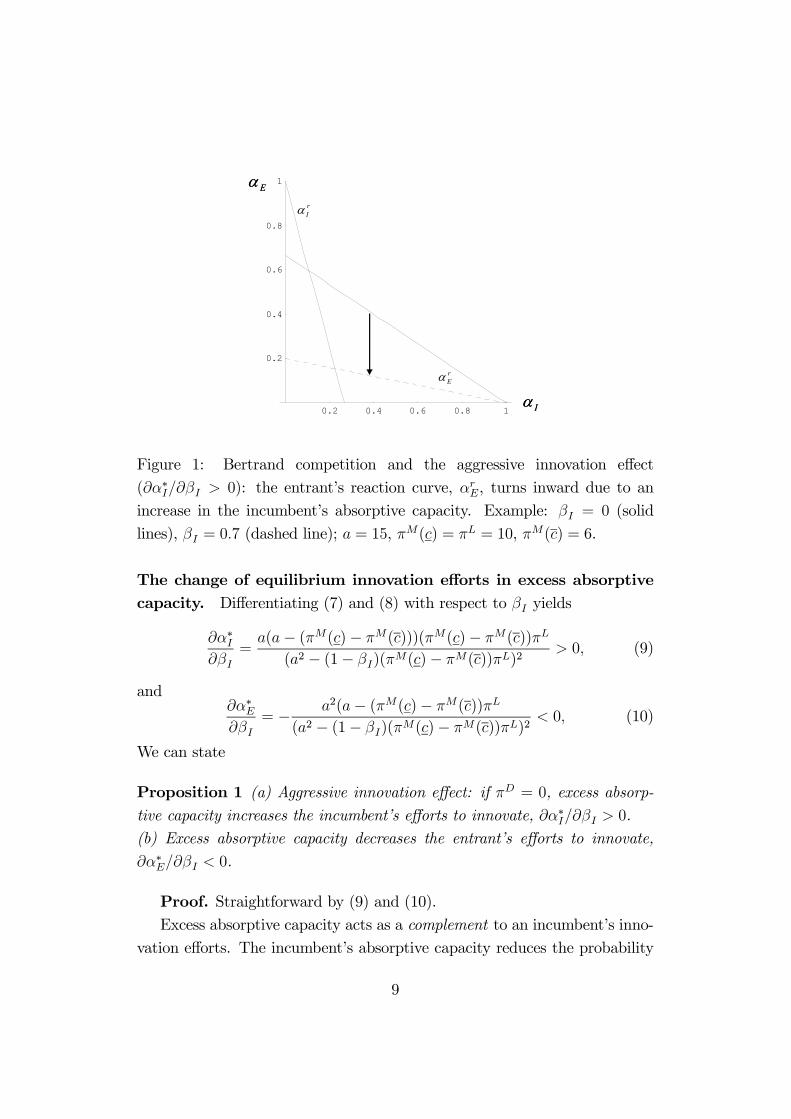
0.2 0.4 0.6 0.8 1
0.2
0.4
0.6
0.8
1
Iα
Eα
rEα
rIα
0.2 0.4 0.6 0.8 1
0.2
0.4
0.6
0.8
1
Iα
Eα
rEα
rIα
Figure 1: Bertrand competition and the aggressive innovation effect
(∂α∗I/∂βI > 0): the entrant’s reaction curve, αrE, turns inward due to an
increase in the incumbent’s absorptive capacity. Example: βI = 0 (solid
lines), βI = 0.7 (dashed line); a = 15, πM(c) = πL = 10, πM(c) = 6.
The change of equilibrium innovation efforts in excess absorptivecapacity. Differentiating (7) and (8) with respect to βI yields
∂α∗I∂βI
=a(a− (πM(c)− πM(c)))(πM(c)− πM(c))πL
(a2 − (1− βI)(πM(c)− πM(c))πL)2
> 0, (9)
and∂α∗E∂βI
= − a2(a− (πM(c)− πM(c))πL
(a2 − (1− βI)(πM(c)− πM(c))πL)2
< 0, (10)
We can state
Proposition 1 (a) Aggressive innovation effect: if πD = 0, excess absorp-tive capacity increases the incumbent’s efforts to innovate, ∂α∗I/∂βI > 0.(b) Excess absorptive capacity decreases the entrant’s efforts to innovate,
∂α∗E/∂βI < 0.
Proof. Straightforward by (9) and (10).Excess absorptive capacity acts as a complement to an incumbent’s inno-
vation efforts. The incumbent’s absorptive capacity reduces the probability
9

that the entrant captures, after a successful innovation, the profits of a cost-
or quality-leader, πL, which decreases the marginal profitability of the en-
trant’s innovation efforts. The reduction of the entrant’s innovation efforts in
turn increases the probability of a unique innovation by the incumbent which
secures monopoly profits, πM(c). It is worth emphasizing that here excess
absorptive capacity has the purely strategic value of deterring an entrant’s
innovation (and entry, respectively). The incumbent itself gains nothing from
its absorptive capacity, i.e. πD = 0, once the entrant has in fact innovated.
Which firm will innovate with a higher probability? Note that (7)
and (8) have identical denominators and hence, by the numerators, α∗I−α∗E <
0 if and only if
πM(c)− πM(c)− (1− βI)πL < 0, (11)
which implies the following
Proposition 2 If πD = 0, the entrant innovates with a higher probability
than the incumbent, α∗E > α∗I , if and only if
βI <πL − (πM(c)− πM(c))
πL.
There exists a ’limit absorptive capacity’ in the sense that α∗E = 0 if and onlyif βI = 1.
Proof. Straightforward by (11) (first claim) and (8) (second claim).To understand the intuition behind Proposition 2 it is useful to begin
with a special case:
Corollary 1 In the case of a drastic innovation, πL = πM(c), the entrant
innovates with a higher probability than the incumbent, α∗E > α∗I , if and onlyif
βI <πM(c)
πM(c).
Due to Reinganum (1983) it has been well established that an entrant has
greater incentives to innovate than an incumbent, provided the innovation is
drastic (or if the entrant, at least, captures a sufficiently high share of the
10

post-innovation market) and there is uncertainty in the innovation process.
Corollary 1 meets these conditions and, indeed, confirms Reinganum’s result
in case there exists no excess absorptive capacity, βI = 0. However, since
πM(c)/πM(c) < 1, Corollary 1 also establishes that a certain degree of excess
absorptive capacity, βI 6 1, suffices to make the incumbent more innovativethan the entrant. How does this happen?
Recall that the assumption of a drastic innovation eliminates Gilbert and
Newberry’s (1982) efficiency effect according to which the entrant lacks some
incentives to innovate because, unlike the incumbent, it does not monopolize
the post-innovation market if it innovates successfully. Excess absorptive ca-
pacity essentially revitalizes Gilbert and Newberry’s argument because the
threat of an immediate imitation reduces the expected value of the entrant’s
innovation. This way the entrant expects lower values from a successful inno-
vation than the incumbent, even if the innovation itself would be sufficiently
drastic to force the (non-successful) incumbent out of the market.
According to Arrow (1962) the incumbent monopolist also lacks some
incentives to innovate because it only replaces its old profit stream with a
new one. Therefore the smaller its incremental profits from an innovation
(πM(c) − πM(c)), i.e. the stronger the replacement effect, the more excess
absorptive capacity a monopolist needs to commit itself to higher innovation
efforts than the entrant. Indeed if the ratio πM(c)/πM(c) approaches 1 so
must βI . At this limit, in fact, the entrant will not try to innovate at all and
neither would the incumbent, as can easily be checked by (7).
Proposition 2 relaxes the assumption of a drastic innovation and explicitly
accounts for Gilbert and Newberry’s argument that an entrant profits less
from an innovation of a given size than an incumbent, i.e. πL < πM(c).
Due to this effect, of course, the incumbent needs less absorptive capacity to
commit itself to a higher innovation level.
3.2 Non-Bertrand competition and the copycat-effect
Consider now the more general case of πD > 0 and πF > 0, a setting that
would reflect, for instance, Cournot competition or Bertrand competition
with differentiated products. The first-order conditions (3) and (4) then
11
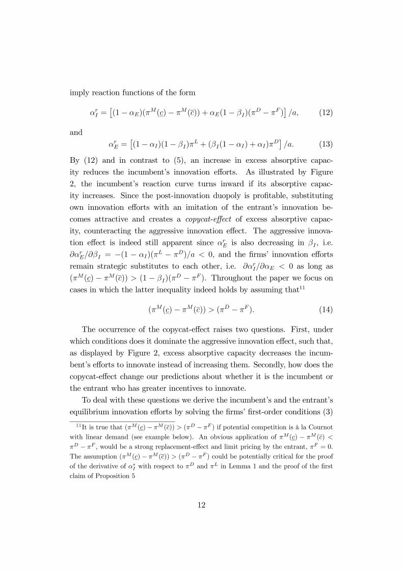
imply reaction functions of the form
αrI =
£(1− αE)(π
M(c)− πM(c)) + αE(1− βI)(πD − πF )
¤/a, (12)
and
αrE =
£(1− αI)(1− βI)π
L + (βI(1− αI) + αI)πD¤/a. (13)
By (12) and in contrast to (5), an increase in excess absorptive capac-
ity reduces the incumbent’s innovation efforts. As illustrated by Figure
2, the incumbent’s reaction curve turns inward if its absorptive capac-
ity increases. Since the post-innovation duopoly is profitable, substituting
own innovation efforts with an imitation of the entrant’s innovation be-
comes attractive and creates a copycat-effect of excess absorptive capac-
ity, counteracting the aggressive innovation effect. The aggressive innova-
tion effect is indeed still apparent since αrE is also decreasing in βI , i.e.
∂αrE/∂βI = −(1 − αI)(π
L − πD)/a < 0, and the firms’ innovation efforts
remain strategic substitutes to each other, i.e. ∂αrI/∂αE < 0 as long as
(πM(c) − πM(c)) > (1 − βI)(πD − πF ). Throughout the paper we focus on
cases in which the latter inequality indeed holds by assuming that11
(πM(c)− πM(c)) > (πD − πF ). (14)
The occurrence of the copycat-effect raises two questions. First, under
which conditions does it dominate the aggressive innovation effect, such that,
as displayed by Figure 2, excess absorptive capacity decreases the incum-
bent’s efforts to innovate instead of increasing them. Secondly, how does the
copycat-effect change our predictions about whether it is the incumbent or
the entrant who has greater incentives to innovate.
To deal with these questions we derive the incumbent’s and the entrant’s
equilibrium innovation efforts by solving the firms’ first-order conditions (3)
11It is true that (πM (c)− πM (c)) > (πD − πF ) if potential competition is à la Cournot
with linear demand (see example below). An obvious application of πM (c) − πM (c) <
πD − πF , would be a strong replacement-effect and limit pricing by the entrant, πF = 0.The assumption (πM (c)− πM (c)) > (πD − πF ) could be potentially critical for the proofof the derivative of α∗I with respect to π
D and πL in Lemma 1 and the proof of the firstclaim of Proposition 5
12

0.2 0.4 0.6 0.8 1
0.2
0.4
0.6
0.8
1
Iα
Eα rIα
rEα
0.2 0.4 0.6 0.8 1
0.2
0.4
0.6
0.8
1
Iα
Eα rIα
rEα
Figure 2: Non-Bertrand competition and dominance of the copycat effect
(∂α∗I/∂βI < 0): the entrant’s and the incumbent’s reaction curves, αrE and
αrI , turn inward due to an increase in the incumbent’s absorptive capacity.
Example: βI = 0 (solid lines), βI = 0.7 (dashed lines); a = 15, πM(c) =
πL = 10, πM(c) = 6, πD = 4, πF = 1.
and (4) simultaneously for
α∗I =a(πM(c)− πM(c))− Ω(πL − βI(π
L − πD))
a2 − Ω(1− βI)(πL − πD)
(15)
and
α∗E =a(πL − βI(π
L − πD))− (1− βI)(πM(c)− πM(c))(πL − πD)
a2 − Ω(1− βI)(πL − πD)
, (16)
where
Ω = (πM(c)− πM(c))− (1− βI)(πD − πF ), (17)
and 0 < Ω < a by (14). The fact that Ω < a also implies that the denomi-
nators of (15) and (16) are strictly positive.
For the analysis to follow it is convenient to have the following interme-
diate results at hand:
Lemma 1 (a) The incumbent’s equilibrium innovation efforts, α∗I, are in-creasing in πM(c) and decreasing in πM(c), πL, πD and πF ,
13

(b) the entrant’s equilibrium innovation efforts, α∗E, are decreasing in πM(c)
and increasing in πM(c), πL, πD and πF .
Proof. See Appendix.The logic behind Lemma 1 can be deduced from a firm’s individual incen-
tive to innovate and the fact that innovation efforts are strategic substitutes.
In particular an increase in πM(c) increases the profit stream the incumbent
gets on top of its current monopoly profits, πM(c). Hence the incumbent
invests more and, as a consequence of the strategic substitutability, the en-
trant less. This logic applies to an increase in πL and πM(c) respectively. The
entrant increases its innovation efforts if πD gets larger because in the case
of a profitable post-innovation duopoly it profits from its innovation even if
the incumbent also innovates or imitates. The increase of α∗E in πD again
causes α∗I to decrease in πD. In order to understand the change of α∗I in πF
note the incumbent’s incentives to innovate are not only driven by the profit
it gains from an innovation if the entrant does not innovate, πM(c)− πM(c),
but also by the probability to obtain πD rather than πF if the entrant inno-
vates successfully. Hence the larger the incumbent’s profits as a follower the
smaller its incentives to innovate with the purpose to get πD instead of πF .
The change of the entrant’s probability to innovate, α∗E, with respect to anincrease in the follower’s profits is, once again, caused by the fact that αI
and αE are strategic substitutes.
The change of equilibrium innovation efforts in excess absorptivecapacity. With respect to the incumbent it is helpful to assume βI = 0
for a second and to think of two sources that create its incentives to in-
novate. First the incumbent seeks to earn incremental monopoly profits
πM(c) − πM(c) > 0 in case the entrant does not innovate successfully. Sec-
ondly, in case the entrant is successful, the incumbent’s own innovation still
secures incremental profits πD − πF > 0 as compared to profits from the old
technology/product, πF . Now, excess absorptive capacity, βI > 0, works as a
substitute to the incumbent’s own innovation in achieving the latter benefit,
πD − πF , which is attainable, just as well, through an imitation. In contrast
excess absorptive capacity complements the incumbent’s own innovation to
accomplish πM(c)− πM(c) by discouraging the entrant from innovating. In
14

essence, the incumbent adopts a copycat (aggressive innovation) strategy if
the substitutional (complementary) effects dominate. We state this more
precisely in
Proposition 3 (a) Dominance of the copycat effect: excess absorptive ca-pacity decreases the incumbent’s efforts to innovate, ∂α∗I/∂βI < 0, if
πM(c)− πM(c)
πD − πF+ 2βI 6
πL
πL − πD+ 1.
(b) Excess absorptive capacity decreases the entrant’s efforts to innovate,
∂α∗E/∂βI < 0.
Proof. See Appendix.As long as the weak inequality in Proposition 3 is satisfied we are guar-
anteed that, in contrast to Proposition 1, excess absorptive capacity is a
substitute to an incumbent’s efforts to innovate. Even though the reverse
statement to Proposition 3 does not follow immediately if the inequality
does not hold we focus on this restricted case as it still captures the main
economic logic.
The left- (LHS) and the right-hand-side (RHS) of the inequality in Propo-
sition 3 balances the strengths of the complementary or substitutional effects
as caused by exogenous (market and technological) conditions. In particu-
lar the LHS accounts for the conditions that directly affect the incumbent’s
innovation incentives as sketched above. Accordingly the larger πD − πF
relative to πM(c)− πM(c) the more likely the incumbent will adopt a copy-
cat strategy and cut back on own innovation efforts as a consequence of its
absorptive capacity.
The RHS takes into account the entrant’s incentives to innovate and, as a
consequence, the relative effectiveness of a copycat or aggressive innovation
strategy by the incumbent. Note first that large leader profits πL increase an
entrant’s incentives to innovate. This makes outspending the entrant on R&D
rather expensive but free-riding on the entrant’s (likely) success attractive:
the incumbent rather adopts a copycat strategy. On the other hand πL−πD
measures the effectiveness of excess absorptive capacity in order to induce
an aggressive innovation strategy: the larger the gap between πL and πD,
15

the more will the incumbent’s absorptive capacity discourage an entrant’s
innovation, which in turn increases the likelihood that the incumbent gets
πM(c) rather than πD after an own successful innovation. This again renders
the incumbent’s innovation efforts more profitable. The lower πL − πD the
more likely will the incumbent adopt a copycat strategy.
The effect of βI in the inequality can be explained as follows. The larger
the incumbent’s absorptive capacity the lower are by part (b) of Lemma 1 the
entrant’s incentives to innovate. Then it is in fact unlikely that the entrant
will be successful at all, hence a copycat strategy becomes less attractive.
Given the fact that a potential entrant’s efforts to innovate always de-
crease in excess absorptive capacity whereas the incumbent’s efforts may
either increase or decrease the question on the net effect of these changes is
apparent. We provide the answer in
Proposition 4 Excess absorptive capacity decreases the firms’ overall inno-vation efforts, ∂(α∗I + α∗E)/∂βI < 0.
Proof. See Appendix.
Which firm will innovate with a higher probability? In the general
case of πD > 0 and πF > 0 the corresponding result to Proposition 2 is
Proposition 5 The entrant innovates with a higher probability than the in-cumbent, α∗E > α∗I, if
βI <πL − (πM(c)− πM(c))
πL − πD.
The higher βI the more likely we have α∗I > α∗E and βI = 1 =⇒ α∗E = (π
D/a),
i.e. there exists no ’limit absorptive capacity’.
Proof. See Appendix.Proposition 5 confirms the main qualitative result of Proposition 2: the
higher the excess absorptive capacity of the incumbent the less likely can we
guarantee that α∗E > α∗I . The difference to Proposition 2 is that the conditionin Proposition 5 depends also on post-innovation duopoly profits, πD. The
denominator reflects, again, how effective an incumbent’s absorptive capacity
16

works as a barrier to innovation and to entry respectively. If and only if the
gap between the entrant’s profit as a cost-leader, πL, and the duopoly profit,
πD, gets sufficiently large, excess absorptive capacity can threaten the entrant
such that it incurs less efforts to innovate than the incumbent.
An example: Potential Cournot Competition with linear demandand constant marginal costs As yet the results stated in Propositions
4 and 5 are not linked to a particular type of product market competition.
This raises the question in which relation the particular profit differences
may stand to each other for a given type of competition and innovation
size. As an example we consider the case of Cournot competition with linear
demand, a − bQ, where Q = qI + qE in the case we calculate πL, πD, πF ,
and Q = qI if we calculate πM(c), πM(c). We suppose, moreover, constant
marginal costs of production, c−xi, i = I,E, where xi 6 a− c measures the
size of the i’th firm’s process-innovation. Note that for πF , πM(c) we have
x = 0. Straightforward algebra, which is omitted for brevity, reveals that the
following relations hold depending on the size of the innovation, x:
minor innovation : πL − πD < πD − πF < πM(c)− πM(c) < πL
major innovation : πD − πF < πL − πD < πM(c)− πM(c) < πL
radical innovation : πD − πF < πM(c)− πM(c) < πL − πD < πL.
The example suggests that it is in particular (πL−πD) which increases in thesize of the innovation. If the innovation is minor then (πL−πD) < (πD−πF )and the incumbent will rather adopt the copycat strategy. However if the
innovation, x, exceeds a certain degree we have (πL − πD) > (πD − πF ) and
eventually even (πL − πD) > (πM(c) − πM(c)). By Proposition 3 drastic
innovations induce an aggressive innovation strategy by the incumbent and,
as confirmed by Proposition 5, monopoly tends to persist in these cases.
17

4 Direct and strategic effects of excess ab-
sorptive capacity (1st stage)
Thus far we have left open the question of how much absorptive capacity will
be built up by an incumbent. In seeking an answer, the difficulty of deter-
mining an appropriate cost measure for absorptive capacity arises. As afore-
mentioned a firm may build up absorptive capacity partly as a by-product
of previous research and partly through specific, extra investments. In our
basic model, therefore, we abstract from such specific costs and restrict our
attention to the direct and strategic effects, which excess absorptive capac-
ity has on the incumbent’s and the entrant’s equilibrium payoffs12. Needless
to say, the incumbent would have to trade off its benefits from absorptive
capacity against the respective costs of building it up.
Effects on the incumbent’s equilibrium payoff The derivative of the
incumbent’s equilibrium payoff VI with respect to βI can be written as
dVIdβI
=∂VI∂βI
+∂VI∂αI
dα∗IdβI
+∂VI∂αE
dα∗EdβI
, (18)
where ∂VI/∂αI = 0 by the second stage maximization problem (envelope the-
orem) and dα∗E/dβI = ∂α∗E/∂βI as given by Proposition 3. We are thus leftwith the direct effect ∂VI/∂βI and the strategic effect (∂VI/∂αE)(dα
∗E/dβI).
Calculating the respective derivatives from (1) and substituting these into
(18) yields
dVIdβI
= α∗E(1− α∗I)(πD − πF )| z
direct copycat effect, >0
(19)
−α∗I(πM(c)− πD)| z
success benefit
+ (1− α∗I)(πM(c)− βIπ
D − (1− βI)πF )| z
failure benefit
dα∗EdβI<0| z
strategic deterrence effect, >0
.
According to (19) the incumbent benefits from more absorptive capacity for
two reasons. As indicated by the first effect, the incumbent firm profits di-12In the terminology of Fudenberg and Tirole (1984) we are analyzing the effects of excess
absorptive capacity in the case of entry accommodation and entry deterrence respectively.
18

rectly because it receives incremental profits (πD − πF ) if only the entrant
innovates successfully. On the other hand more absorptive capacity also ben-
efits the incumbent for strategic reasons: decreasing the entrant’s incentives
to innovate, ∂α∗E/∂βI < 0, pays off because the incumbent firm then receivesπM(c) > πD if it innovates successfully and πM(c) > βIπ
D + (1 − βI)πF if
it fails to innovate. This positive strategic effect indicates that an incum-
bent over-invests in its absorptive capacity13. Without costs of absorptive
capacity VI is indeed maximized at βI = 1.
Effects on the entrant’s equilibrium payoff Proceeding in a similar
way as above, we obtain
dVEdβI
=∂VE∂βI
+∂VE∂αE
dα∗EdβI
+∂VE∂αI
dα∗IdβI
, (20)
where, again, ∂VE/∂αE = 0 and dα∗I/dβI = ∂α∗I/∂βI as given by Proposition3. Calculating the respective derivatives from (2) and rearranging terms
slightly gives
dVEdβI
= −α∗E(πL − πD)
·(1− α∗I) + (1− βI)
dα∗IdβI
¸< 0. (21)
Of course, excess absorptive capacity only affects the entrant’s equilibrium
payoff in case it succeeds in innovating, that is with probability α∗E. Thenexcess absorptive capacity reduces the entrant’s payoff by (πL−πD), i.e. the
incremental profit of being a cost- or quality-leader instead of a symmetric
duopoly competitor. By the square bracketed expression in (21) this effect is
contingent on two cases. First, if the incumbent does not innovate success-
fully, i.e. with probability (1 − α∗I), an additional unit of excess absorptivereduces the potential entrant’s payoff simply because it increases the proba-
bility of an immediate imitation (by one unit). However, even if the incum-
bent does not imitate successfully, (1 − βI), excess absorptive capacity still
13Benoit and Krishna (1991) show that preemptive capacity may facilitate entry indynamic competition by increasing competitive intensity and, as a consequence, making acollusive outcome more sustainable. Hence if post-innovation competition is dynamic andpreemptive absorptive capacity increases competitive intensity one might derive differentconclusions regarding the incumbent’s incentives to over-invest.
19

affects the entrant’s payoff as it changes the incumbent’s innovation behavior,
dα∗I/dβI . If the aggressive innovation effect dominates, dα∗I/dβI > 0, the for-
mer is substantiated, whereas, if the copycat effect dominates, dα∗I/dβI < 0,it is weakened. In any case the square bracketed expression remains positive
such that the overall effect of excess absorptive capacity on the entrant’s equi-
librium payoff is certainly negative (see appendix). Thus excess absorptive
capacity constitutes a barrier to entry. We summarize these considerations
in
Proposition 6 Excess absorptive capacity increases (decreases) the incum-bent’s (entrant’s) second stage equilibrium payoff.
Proof. See appendix.
5 Conclusion
As an alternative to studies that focus on how an incumbent’s superior ability
to innovate preserves its dominant position, this paper analyzes an incum-
bent’s superior ability to imitate, i.e. its excess absorptive capacity, as a
means of deterring an external innovation and entry respectively. The con-
cept of excess absorptive capacity allows to relax assumptions of initial tech-
nological leads by the incumbent as well as first-mover-advantages in innova-
tion. Yet even without these assumptions our results indicate that monopoly
tends to persist. First we show that excess absorptive capacity always de-
creases the entrant’s incentives to innovate whereas it increases (decreases)
the incumbent’s incentives if potential duopoly profits are low (high). In any
case a larger excess absorptive capacity ensures that the incumbent tends
to innovate with a higher probability than the entrant. Secondly we find
excess absorptive capacity to increase (decrease) the incumbent’s (entrant’s)
equilibrium payoffs.
Our paper suggests a number of extensions. First some of our (main)
conclusions hinge on the fact that innovation efforts are strategic substi-
tutes. If one defines innovation efforts as a flow of investments rather than
an up-front expenditure, however, the firms’ strategic variables are (often)
20

complements14 and it has to be validated in how far our results remain true
in these cases15. Closely related, secondly, we applied a static set-up for
something dynamic in nature. For a dynamic R&D race with knowledge ac-
cumulation Doraszelski (2003) derives simulation results that suggest firms
invest more aggressively if they have a large knowledge stock. This bears
resemblance to our aggressive innovation finding but seems to jar with the
outcome of the copycat strategy. It appears worthwhile to integrate the ad-
vantages of both set-ups, an explicit formulation of absorptive capacity and
the multistage nature of the Doraszelski (2003) model. Thirdly Hoppe et al.
(2005) identify free-riding effects among several incumbents who bid for a li-
cense in order to prevent entrants from obtaining the license. Similar to their
context in which each incumbent is willing to avoid entry but would rather
prefer the other incumbent to pay the price of preemption, in our model sev-
eral incumbents might rely on each other to bear the costs of maintaining an
excess absorptive capacity.
Acknowledgements I would like to thank Werner Bönte, Tom Gre-
sik, Heidrun Hoppe, Stefan Napel and Wilhelm Pfähler for very helpful com-
ments. Thanks are also due to Ludwig Burger, Johannes Bruder and Nina
Carlsen.
14See Martin (1999) for an overview of R&D games with strategic substitutes and com-
plements.15Chen (2000) shows that an incumbent’s and an entrant’s innovation investments de-
pend crucially on whether the new product is a strategic substitute or complement to themonopolists old product.
21

Appendix
Proof of Lemma 1. For notational convenience let fI = 0 and fE = 0
denote the incumbent’s and the entrant’s first-order conditions as given by
(3) and (4) which are satisfied in α∗I and α∗E as given by (15) and (16). Then
we have by the implicit function rule and Cramer’s rule that
∂α∗i∂Π
=
¯JΠi
¯|J | , i = I,E, Π = πM(c), πM(c), πL, πD, πF ,
where |J | is the Jacobian determinant of the equation system fI = 0 and
fE = 0,
|J | =¯¯ ∂fI/∂αI ∂fI/∂αE
∂fE/∂αI ∂fE/∂αE
¯¯
= (∂fI/∂αI)(∂fE/∂αE)− (∂fI/∂αE)(∂fE/∂αI)
= a2 − Ω(1− βI)(πL − πD) > 0, (22)
where Ω is given by (17), 0 < Ω < a by (14), and¯JΠi
¯is the determinant of
the Jacobian with the i’th column replaced with partial derivatives,−∂fi/∂Π.In particular¯
JπM (c)I
¯=
¯¯ −∂fI/∂πM(c) ∂fI/∂αE
−∂fE/∂πM(c) ∂fE/∂αE
¯¯ = a(1− α∗E) > 0,
which implies, as |J | > 0 by (22), that ∂α∗i /∂πM(c) > 0. Respectively we
obtain¯JπM (c)I
¯= −a(1− α∗E)⇒ ∂α∗I/∂π
M(c) < 0¯JπL
I
¯= −(1− α∗I)(1− βI)Ω⇒ ∂α∗I/∂π
L < 0¯JπD
I
¯= −aα∗E(πD − πF )− (α∗I(1− βI) + βI)Ω⇒ ∂α∗I/∂π
D < 0¯JπF
I
¯= −a(1− βI)α
∗E ⇒ ∂α∗I/∂π
F < 0.
This establishes part (a).
Next we calculate¯JπM (c)E
¯=
¯¯ ∂fI/∂αI −∂fI/∂πM(c)∂fE/∂αI −∂fE/∂πM(c)
¯¯
= −(1− a∗E)(1− βI)(πL − πD)⇒ ∂α∗E/∂π
M(c) < 0.
22

Proceeding in a similar fashion yields¯JπM (c)E
¯= (1− a∗E)(1− βI)(π
L − πD)⇒ ∂α∗E/∂πM(c) > 0,¯
JπL
E
¯= a(1− α∗I)(1− βI)⇒ ∂α∗E/∂π
L > 0,¯JπD
E
¯= a(α∗I(1− βI) + βI) + α∗E(1− βI)(π
D − πF )(πL − πD)
⇒ ∂α∗E/∂πD > 0,¯
JπF
E
¯= (−1 + βI)
2α∗E(πL − πD)⇒ ∂α∗E/∂π
F > 0
This establishes part (b).¥
Proof of Proposition 3. Unfortunately implicit differentiation as in the
proof of Lemma 1 does not reveal the sign of ∂α∗I/∂βI and ∂α∗E/∂βI respec-tively. Therefore we need to consider equilibrium innovation efforts, α∗I andα∗E, as given by (15) and (16) explicitly. In doing so let NI and D denote the
numerator and the denominator of (15). Then
∂α∗I∂βI
=(∂NI/∂βI)D − (∂D/∂βI)NI
D2, (23)
where
∂NI
∂βI= (πM(c)−πM(c))(πL−πD)−(πD−πF ) £2πL(1− βI)− πD(1− 2βI)
¤,
and∂D
∂βI=£(πM(c)− πM(c))− 2(1− βI)(π
D − πF )¤(πL − πD).
Note that
∂NI/∂βI − ∂D/∂βI
= (πD − πF )©2(1− βI)(π
L − πD)− [2πL(1− βI)− πD(1− 2βI)]ª
= −(πD − πF )πD
and hence ∂NI/∂βI < ∂D/∂βI . Now suppose that ∂NI/∂βI 6 0. On the
one hand, if ∂D/∂βI > 0 then ∂α∗I/∂βI is unambiguously negative, becauseD > 0 ∧ N > 0. On the other hand, if ∂D/∂βI < 0 then ∂α∗I/∂βI < 0
23

because ∂D/∂βI < 0 =⇒ |∂NI/∂βI | > |∂D/∂βI | and D > N . It is the case
that ∂NI/∂βI 6 0 if and only if
πM(c)− πM(c)
πD − πF6£2πL(1− βI)− πD(1− 2βI)
¤πL − πD
which can be re-written as
πM(c)− πM(c)
πD − πF6 πL + (πL − πD)(1− 2βI)
πL − πD
⇐⇒ πM(c)− πM(c)
πD − πF+ 2βI 6 πL
πL − πD+ 1.
This establishes the first claim.
Second claim.∂α∗E∂βI
= − 1
D2(πL − πD)Φ,
where
Φ = a3 − a2(πM(c)− πM(c)) (24)
+(−1 + βI)2(πM(c)− πM(c))(πL − πD)(πD − πF )
+a((πM(c)− πM(c))πD − (1− βI)(πD − πF )(πD(1 + βI) + πL(1− βI)).
Note that ∂α∗E/∂βI is negative as long as Φ is positive. We have that
∂Φ
∂πM(c)= −a(a− πD) + (−1 + βI)
2(πL − πD)(πD − πF ) < 0
because a > (πD − πF ) ∧ (a− πD) > (πL − πD) and respectively
∂Φ
∂πM(c)= a(a− πD)− (−1 + βI)
2(πL − πD)(πD − πF ) > 0.
We set πM(c) = a and ∂πM(c) = 0 in order to evaluate Φ below its minimum
level:
Φ¯πM (c)=a, πM (c)=0 = aπD(a− 2(1− βI)(π
D − πF )) > 0,
because a > πM(c) > 2πD. (Second claim).¥
24

Proof of Proposition 4. By similar arguments as in the proof of Lemma
1 we derive¯JβII
¯= (1− α∗I)(π
L − πD)Ω− aα∗E(πD − πF )¯
JβIE
¯= (α∗E(1− βI)(π
D − πF )− a(1− α∗I)(πL − πD),
to establish, after some re-arrangements, that¯JβII
¯+¯JβIE
¯= −α∗E(πD − πF )(a− (1− βI)(π
L − πD)
−(1− α∗I)(πL − πD)(a− Ω)
⇒ ∂α∗I/∂βI + ∂α∗E/∂βI < 0.
¥
Proof of Proposition 5. First claim. Letting NI and NE still denote the
numerators of (15) and (16) we have that sign(α∗I−α∗E)⇐⇒ sign(NI−NE).
After some re-arrangements we can write
NI −NE = a©(πM(c)− πM(c))− (πL − βI(π
L − πD))ª
−©(1− βI)(πL − πD)(πM(c)− πM(c)) + Ω(πL − βI(π
L − πD))ª,
where the first curly bracketed term is negative if and only if
βI <πL − (πM(c)− πM(c))
πL − πD,
and the second curly bracketed term is strictly positive. This establishes the
first claim.
The second claim follows by
∂(NI −NE)
∂βI= −a(πL − πD)− (πD − πF )(2πL(1− βI)− πD(1− 2βI)) < 0,
and the third claim follows straightforwardly upon setting βI = 1 in (16).¥
Proof of Proposition 6. First claim (the incumbent’s equilibrium pay-
off). Straightforward by (19).
Second claim (the entrant’s equilibrium pay-off). By (21), dVE/dβI < 0
if Ψ = (1− α∗I) + (1− βI)(dα∗I/dβI) > 0. By (15) and (23) we can compute
Ψ = aΦ/D2 > 0, where D still denotes the denominator of (15) and Φ > 0
is given by (24) in the proof of Proposition 4, second claim.¥
25

References
[1] Arrow, K.J., (1962). Economic welfare and the allocation of resources
for invention. In: Nelson, R. (Ed.). The Rate and Direction of Inventive
Activity. Princeton University Press, 609-624.
[2] Benoit, J.-P., Krishna, V. (1991). Entry deterrence and dynamic com-
petition. International Journal of Industrial Organization, 9, 477-495.
[3] Blundell, R., Griffith, R. (1999). Market Share, Market Value and Inno-
vation in a Panel of British Manufacturing Firms. Review of Economic
Studies, 66, 529-555.
[4] Bulow, J., Geanakoplos, J., Klemperer, P. (1985). Multimarket
oligopoly, strategic substitutes and complements. Journal of Political
Economy, 93, 448-511.
[5] Chen, Y. (2000). Strategic Bidding by Potential Competitors: Will
Monopoly Persist?. Journal of Industrial Economics, XLVIII, 161-175.
[6] Cohen, W. M., Levinthal, D. A. (1989). Innovation and learning: The
two faces of R&D. The Economic Journal, 99, 569-596.
[7] Cohen, W. M., Levinthal, D. A. (1990). Absorptive Capacity: A New
Perspective on Learning and Innovation. Administrative Science Quar-
terly, 35, 128-152.
[8] Cohen, W. M., Levinthal, D. A. (1994). Fortune Favors the Prepared
Firm. Management Science, 40, 227-251.
[9] Czarnitzki, D., Kraft, K. (2004). An empirical test of asymmetric models
on innovative activity: who invests more into R&D, the incumbent or
the challenger? Journal of Economic Behavior & Organization, 54, 153-
173.
[10] Doraszelski, U. (2003). An R&D race with knowledge accumulation.
RAND Journal of Economics, 34, 20-42.
26

[11] Etro, F. (2004). Innovation by Leaders. The Economic Journal, 114,
281-303.
[12] Fudenberg, D., Tirole, J. (1984). The Fat-Cat Effect, the Puppy-Dog
Ploy, and the Lean and Hungry Look. American Economic Review, 74,
361-366.
[13] Gilbert, R. J., Katz, M. L. (2001). An Economist’s Guide to U.S. v.
Microsoft. Journal of Economic Perspectives, 15, 25-44.
[14] Gilbert, R. J., Newberry, D. M. G. (1982). Preemptive Patenting and
the Persistence of Monopoly. American Economic Review, 72, 514-526.
[15] Griliches, Z. (1992). The Search for R&D Spillovers. Scandinavian Jour-
nal of Economics, 94, S29-S47.
[16] Henderson, R., Cockburn, I. (1996). Scale, Scope, and Spillovers: The
Determinants of Research Productivity in Drug Discovery. Rand Journal
of Economics, 27, 32-59.
[17] Hoppe, H. C., Jehiel, P., Moldevanu, B. (2005). License Auctions and
Market Structure. Journal of Economics and Management Strategy,
forthcoming.
[18] Joglekar, P., Bohl, A. H., Hamburg, M. (1997). Comments on "Fortune
Favors the Prepared Firm". Management Science, 43, 1455-1463.
[19] Kanniainen, V., Stenbacka, R. (2000). Endogenous Imitation and Impli-
cations for Technology Policy. Journal of Institutional and Theoretical
Economics, 156, 360-381.
[20] Klein, B. (2001). The Microsoft Case: What Can a dominant Firm Do
to Defend Its Market Position? Journal of Economic Perspectives, 15,
45-62.
[21] Martin, S. (1999). Advanced Industrial Economics. fourth edition,
Blackwell, Oxford.
27

[22] Reinganum, J. F. (1983). Uncertain Innovation and the Persistence of
Monopoly. American Economic Review, 73, 741-748.
[23] Rosen, R. J. (1991). Research and development with asymmetric firm
sizes. RAND Journal of Economics, 22, 411-429.
[24] Rosenberg, N. (1990). Why do firms do basic research (with their own
money)? Research Policy, 19, 165-174.
[25] Tirole, J. (1988). The Theory of Industrial Organization. MIT Press,
Cambridge, Massachusetts.
28

Knowledge Transfer in
Buyer-Supplier Relationships
- When It (Not) Occurs
Werner Bönte and Lars Wiethaus
June 2005
Abstract
A buyer’s technical knowledge may increase the efficiency of its
supplier. Suppliers, however, frequently maintain relationships with
additional buyers. Knowledge disclosure then bears the risk of benefit-
ing one’s own competitor due to opportunistic knowledge transmission
through the common supplier. We show that in one-shot relationships
no knowledge disclosure takes place because the supplier has an incen-
tive for knowledge transmission and, in anticipation of this outcome,
buyers refuse to disclose any of their knowledge. In repeated relation-
ships knowledge disclosure is stabilized by larger technological prox-
imity between buyers and suppliers and destabilized by the absolute
value of the knowledge.
JEL Classification: O31, O32, L13, L20Keywords: Knowledge Transfer; Knowledge Spillovers; Cooperation;Innovation; Repeated Games.
1
1 Introduction
Knowledge sharing among vertically related firms is commonly regarded as a
key ingredient to efficient buyer-supplier relationships. In particular, the dis-
closure of technical knowledge1 by a customer may increase the supplier’s pro-
duction efficiency. Kotabe et al. (2003) document this positive effect empir-
ically for suppliers in the U.S. and Japanese automotive industry. Moreover,
increasing supplier performance usually translates into lower input prices or
enhanced input quality respectively.2 Thus, buyers indeed have an incentive
to disclose their technical knowledge to their suppliers.3
Frequently, however, firms purchase inputs from the same suppliers as
their rivals. If a common supplier is either not able or not willing to treat
obtained knowledge confidentially, the leakage of knowledge to rivals may
dampen or even outweigh the gains from an increased supplier performance.
According to empirical evidence such concerns are ubiquitous. Grindley,
Mowery and Silverman (1994) report that manufacturers of semiconductor
materials and equipment (SME) were concerned over sharing information
with members of SEMATECH (the Semiconductor Manufacturing Technol-
ogy Consortium) because they feared the disclosure of proprietary informa-
tion to their competitors. Cassiman and Veugelers (2002) and Bönte and
Keilbach (2005) find that firms which cannot protect their proprietary inno-
vations by strategic protection mechanisms, such as complex or idiosyncratic
production processes, have a lower propensity to engage in knowledge sharing
R&D cooperations with their suppliers.4
1Alternative types of valuable knowledge in vertical relationships are demand and costinformation, see Lee and Whang (2000) for a survey of supply chain information sharing.
2For instance, Dyer and Hatch (2004 a, b) relate Toyota’s superior quality- and profitperformance to its more intense knowledge sharing with suppliers as compared to GeneralMotors, Ford and Daimler-Chrysler.
3Of course, a supplier may also have an incentive to disclose its knowledge to customers.Harhoff (1996), for instance, shows that a monopolist supplier may voluntarily disclose
knowledge to customers in order to induce process and product innovations by customers,which in turn may enhance the demand for the supplier’s intermediate good.
4Firms may also engage in horizontal knowledge sharing with firms from the sameindustry. Empirical evidence suggests that such direct transfer occurs (Appleyard 1996,Sattler et al. 2003, Schrader, 1991). Jost (2005) investigates theoretically the limits of
2

Of course, suppliers will try to meet such objections. Consider, for exam-
ple, the electronic manufacturer Flextronics who builds products for a bunch
of high-tech firms, including direct competitors such as Motorola and Eric-
sson. According to Flextronics’ management the company “had been able
to erect ‘fire walls’ to prevent proprietary information from leaking between
competitors”.5 The credibility of such promises, however, is questionable
if the supplier benefits from knowledge transmission. Then the disclosed
knowledge may be opportunistically misappropriated by the supplier, which
immediately raises the question of how much knowledge the buyer should
disclose in the first place.
We seek answers to these questions by employing a four stage model. In
the first stage two downstream firms, i.e. buyers, decide how much of their
proprietary technical knowledge they disclose to an upstream monopolist,
i.e. their common supplier. Any disclosed knowledge increases the supplier’s
production efficiency. In the second stage the common supplier decides how
much of one buyer’s knowledge it transfers to the other one. In the third
stage the supplier sets its price, i.e. the buyers’ input price. In the fourth
stage the downstream firms compete in output-quantities. This scenario is
analyzed both for a one-shot buyer-supplier-relationship and for repeated
relationships.
The combination of potential supplier opportunism and downstream com-
petition is the key ingredient to our knowledge sharing model. Only few pre-
vious studies consider these issues. Baiman and Rajan (2002) address the role
of opportunism in buyer-supplier relationships. In contrast to our work they
focus on a bilateral buyer-supplier relationship in which the supplier misap-
propriates the information by using it for himself; for instance, the supplier
may emerge as a competitor to the knowledge sharing buyer. Their setting
thus reflects an arguably stronger and more costly kind of misappropriation
than our knowledge-transfer scenario.
Similar to our setting Li (2002) and Zhang (2002) consider informa-
tion sharing of competing downstream firms to a common supplier. In
their model, however, information is about demand or cost uncertainty. As
such horizontal knowledge sharing networks.5The New York Times 2001, “Ignore the Label, It’s Flextronics Inside”.
3

the supplier takes advantage of these informations to seek more rents from
its buyers, the latter suffer from disclosing their knowledge in any bilat-
eral buyer-supplier relationship. The leakage effect of information from one
downstream firm to another is negative if demand information is at stake
but positive when it comes to cost information. In contrast, the disclosure
of technical knowledge in our model induces a positive effect within the bi-
lateral buyer-supplier relationship (i.e. increased production efficiency and a
lower input price) whereas the leakage of technical knowledge always hurts
(benefits) the revealing (receiving) downstream firm.
Harhoff et al. (2003) propose that two downstream firms may reveal
their innovations because their common supplier may refine them. Yet re-
finements are only profitable in the case that both downstream firms adopt
the improved innovation. This in turn causes a downstream firm to reveal
its innovation if and only if it expects the other downstream firm to adopt
it too. Our study is in contrast motivated by the above mentioned empirical
studies that suggest firms to disclose their innovation specifically if these can-
not be adopted too easily by their competitor or if the innovation is treated
confidentially by the supplier respectively.
Our study extends the scope of previous works as we analyze explicitly
the supplier’s incentive to behave opportunistically. Moreover, to behave op-
portunistically either in a one-shot buyer-supplier relationship or in repeated
relationships. Our results suggest that this distinction is crucial to under-
stand knowledge disclosure in buyer-supplier relationships. In particular we
find that a buyer discloses its technical knowledge completely as long as
the common supplier does not further transfer ‘too much’ of that knowledge
to the other downstream firm. The supplier, however, has an incentive to
give away all of its knowledge to downstream firms. The announcement to
treat the obtained knowledge confidentially (e.g. to install ‘firewalls’) is thus
not credible6 (not a subgame perfect equilibrium) and, anticipating that, a
downstream firm will not disclose any of its knowledge in the first place.7
6Miliou (2004) investigates the welfare effects of firewalls in a setting with exogenousspillovers from a buyer to a vertically integrated supplier. However, he leaves open thequestion of whether the supplier has an incentive to install a firewall.
7Thereby our results also indicate that the case of full knowledge sharing as analyzed
4

These predictions change if the buyer can threaten not to disclose its
knowledge in subsequent periods. We identify two types of knowledge sharing
equilibria in the repeated game. In the first one each buyer discloses its
knowledge completely whereby the supplier does not further transfer ‘too
much’ of it. In the second, more subtle one, each buyer, again, discloses
its knowledge completely but the supplier further transfers all of it. This
equilibrium occurs because revealing and receiving knowledge implies a net
benefit for the downstream firms. Here, in fact, one buyer threatens the
other one by not disclosing its knowledge in future periods if it did not
receive an adequate amount of knowledge in return. Both types of equilibria
are stabilized by a larger technological proximity between the buyers and the
supplier and destabilized by the absolute value of knowledge.
The paper is arranged as follows. In section 2 we set up the model. In
particular we derive the downstream firms’ optimal output quantities in the
fourth stage and the supplier’s input price in the third stage of the model.
In section 3 we analyze the downstream firms’ incentives for knowledge dis-
closure in a one-shot relationships. In section 4 we investigate the case in
which firms interact repeatedly. Section 5 concludes.
2 The Basic Model
We consider two vertically related industries where two firms in the down-
stream industry, i = 1, 2 transform the intermediate input produced by the
upstream industry into a final output. The upstream industry is character-
ized by a monopolist supplier, u, as we are essentially interested in the case
in which downstream competitors are related to a common supplier.
Our model consists of four stages. In the first stage each downstream firm
(buyer) decides how much of its proprietary knowledge it discloses to the up-
stream monopolist (supplier). This knowledge transfer lowers the supplier’s
production costs. Once the upstream firm possesses the new knowledge,
from i say, it decides in the second stage, whether it further transfers this
knowledge to j. In the third stage the upstream firm sets the intermediate
by Ishii (2004) will not be an equilibrium.
5

input price and in the fourth stage the downstream firms compete in the final
output market a la Cournot.
The upstream firm produces with marginal costs of production, c − Y,
where c is an exogenous parameter, c > Y , and
Y = t(αixi + αjxj), i = 1, 2, i 6= j (1)
represents the amount of cost-reduction the upstream firm realizes due to
the knowledge transfer of the downstream firms. In particular xi (xj) mea-
sures the size of i’s ( j’s) proprietary knowledge. The endogenous variables
αi ∈ (0, 1), i = 1, 2, represent the fraction of knowledge the downstream
firms actually disclose to u. The upstream firm’s benefit from any amount of
the downstream industry’s knowledge, however, might be technologically lim-
ited. The parameter t ∈ (0, 1) captures the degree of technological proximitybetween the upstream firm and the downstream firms.
The downstream firms’ marginal costs of production are A+w−Xi, where
A is an exogenous parameter, A > Xi, w is the intermediate input price and
Xi = xi + βiαjxj, i = 1, 2, i 6= j (2)
is the amount of cost-reduction each downstream firm realizes due to the sum
of its own proprietary knowledge, xi, and the fraction of its rival’s knowledge,
xj, that gets into its domain. The ith firm receives its rival’s knowledge
according to the fraction αj, the rival has previously revealed to the upstream
monopolist and the fraction βi ∈ (0, 1), i = 1, 2, that is transferred from firmj’s knowledge to firm i via the common supplier. According to equation (2)
the ith downstream firm will utilize all of its rival’s knowledge if αj = βi = 1.
This implies that these firms have chosen to follow the same technological
trajectories in the first place. This presumption is in line with a recent finding
of Wiethaus (2005) who shows that competing firms indeed tend to adopt
identical R&D approaches8. Since we are interested in firms’ incentives to
disclose their proprietary knowledge but not in their incentives to create that
knowledge we will assume throughout the rest of the paper that both firms
8He also extends this finding to Kamien and Zang’s (2000) model according which theauthors had previously predicted that competing firms adopted different R&D approaches.
6

possess an innovation of given and identical size: x = xi = xj9.
We summarize these considerations in the firms’ profit functions. The ith
downstream firm’s profit-function can be written as
πi = (P (Q)− (A+ w −Xi))qi, i = 1, 2 (3)
where P (Q) = a− bQ determines the price of the final product as a function
of the firms’ joint output quantity, Q = qi + qj. We assume that both
downstream firms pay the same input price w, i.e. the monopolist supplier
does not differentiate the input price. Without loss of generality we assume
b = 1. Supposing that the final product is produced with a 1:1 technology
(one unit of final product requiring exactly one unit of input) the upstream
firm’s profit-function is
πu = (w − (c− Y ))Q. (4)
Using the standard backwards induction procedure we first derive the
firms’ decisions starting in the fourth stage. Differentiation of (3) with re-
spect to qi and qj respectively and then solving both first-order-conditions
simultaneously for qi and qj yield the firms’ equilibrium output quantities,
q∗i =a−A− w + 2Xi −Xj
3i = 1, 2 i 6= j. (5)
where Xi, and Xj respectively, are given by (2). We assume that the down-
stream firms take the price of the intermediate input w as given.
In the third stage the upstream firm sets the intermediate input price.
Anticipating the downstream firms’ behavior in the final product market the
upstream firm maximizes its profits upon substitution of
Q∗ = q∗i + q∗j =2(a−A− w) +Xi +Xj
3i = 1, 2 i 6= j (6)
forQ in (4). Solving the first-order-condition, ∂πu/∂w|Q=Q∗ = 0, for w yieldsthe intermediate input price
w∗ =2(a−A+ c− Y ) +Xi +Xj
4. (7)
9Firms’ R&D investments have been anaylized extensively by, among others,D’Aspremont and Jacquemin (1988) and Kamien et al. (1992) for the case of horizon-tally related firms and by Atallah (2002) and Ishii (2004) for the case of vertically relatedfirms.
7

By (6) and (7) it is apparent that a decrease of marginal costs in the down-
stream industry due to an increase in knowledge (Xi,Xj) creates an addi-
tional demand effect for the intermediate input which in turn increases the
monopolist’s profit-maximizing price10, ∂w∗/∂Xi > 0, and its profits respec-
tively. If the downstream firms, however, disclose their knowledge to the up-
stream firm this lowers also upstream production costs by Y = t(αix+ αjx)
and, as a consequence, w∗. We will refer to this latter mechanism as the costefficiency effect.
3 Knowledge disclosure in a one-shot rela-
tionship
We will investigate four scenarios when analyzing the remaining stages of the
game: In the first one the parameter β is assumed to be exogenous because
the upstream firm does not deliberately transfer knowledge disclosed by one
downstream firm to the other downstream firm. Therefore, in this scenario
the game reduces to a three-stage game. In the second case the upstream
monopolist decides opportunistically whether or not to transfer the disclosed
knowledge at the second stage. In both scenarios the downstream firm is
supposed to maximize solely its own profits when deciding about disclosure
of knowledge at the first stage. In the third scenario we propose a cooperative
solution between the downstream firm and the upstream monopolist.
Absence of supplier opportunism In this section we analyze a down-
stream firm’s incentive to disclose its knowledge to the upstream monopolist
assuming that the latter does not behave opportunistically.11 In other words
the supplier treats disclosed knowledge confidentially and does therefore not
take any action to pass on the disclosed knowledge to the other downstream
firm.10Banerjee and Lin (2003) point out that this effect raises a rival’s costs and may hence
stimulate downstream firms’ R&D.11A customer’s expectation that a common supplier will not exploit the vulnerabilities
created by knowledge disclosure may be viewed as the customer’s trust in the supplier.See e.g. Bönte (2005).
8

In order to obtain the ith firm’s output quantity we substitute w∗ for win (5) which yields
q∗∗i =2(a−A− c+ Y ) + x(2 + 7αjβi − 5αiβj)
12i = 1, 2 i 6= j, (8)
given the monopolist’s optimal price w∗ and prior to i’s knowledge disclosureto its supplier. The parameters βi and βj take the value zero if the upstream
firm is able to keep the shared knowledge fully secret whereas positive val-
ues reflect the leakage of knowledge to downstream firms that is (here) not
intended by the upstream firm. Making use of (8) and (7) we can write (3)
as
π∗i = (a− (q∗∗i + q∗∗j )− (A+ w∗ −Xi))q∗∗i i = 1, 2 i 6= j. (9)
Differentiating (9) with respect to αi yields
∂πi∂αi
= x(2t− 5βj)2(a−A− c+ Y ) + x(2 + 7αjβi − 5αiβj)
72. (10)
Note that the fraction in (10) is strictly positive which means that the sign
of (2t − 5βj) alone determines whether knowledge transfer to the upstreammonopolist is profitable from a downstream firm’s point of view. We state
this more precisely in
Lemma 1 There exists a critical level of knowledge leakage from the up-
stream firm, u, to the ith firm’s rival j, which determines whether the ith
firm discloses all or nothing of its knowledge to the upstream firm. Denoting
this critical level βcj, we have
βcj >2
5t =⇒ α∗i = 0,
and
βcj <2
5t =⇒ α∗i = 1, i = 1, 2 i 6= j.
Proof. By (10), ∂π/∂αi > 0⇐⇒ 2t− 5βj > 0, for all αi ∈ (0, 1).The intuition for this result is rather straightforward if we look at the
marginal effects of knowledge disclosure by firm i on its own profit and on
the rival’s profit in a more general way:
9

∂πi∂αi
=∂πi∂Xi>0
∂Xi
∂αi=0| z
direct effect=0
+∂πi∂w<0
∂w∗
∂αi(<0)| z
price effect
(>0)
+∂πi∂qj<0
∂q∗∗j∂αi>0| z
strategic effect60
, (11)
∂πj∂αi
=∂πj∂Xj>0
∂Xj
∂αi>0| z
direct effect>0
+∂πj∂w<0
∂w∗
∂αi(<0)| z
price effect
(>0)
(12)
The direct marginal effect of knowledge disclosure on ith firm’s own profit
in equation (11) is zero. Consequently, the decision of the ith firm about the
disclosure of knowledge to the upstream monopolist is driven by a price
effect and a strategic effect. The sign of the price effect in equation (11)
depends on the sign of the change of the intermediate input price: ∂w∗/∂αi =
−14x(2t − βj). This sign will be positive if the cost efficiency effect, 2t,
is stronger than the additional demand effect, −βj. The strategic effect isalways negative because the ith firm’s knowledge reduces j’s production costs
and increases its output quantity respectively: ∂q∗∗j /∂αi =112x(2t + 7βj).
Obviously knowledge disclosure by downstream firms will not occur unless
the price effect is positive.12
Thus, the sign of the marginal effect of knowledge disclosure on firm
i’s own profit is determined by the counteracting (positive) price effect and
(negative) strategic effect. In contrast, the marginal impact of knowledge
disclosure by firm i on the rival’s profit is always positive provided βj 6= 0.The price effect in (12) is positive because the price effect is the same for both
firms and firm i will not have an incentive to disclose knowledge if this effect
is negative or zero. The direct effect is positive because ∂Xj/∂αi = βjx.
Rather counter-intuitively, equations (11) and (12) imply that the ith firm
will disclose its technical knowledge to the upstream monopolist being aware
that this benefits its rival more than itself. However, according to Lemma
1 the rival must not benefit too much. For example, given the parameter t
12The brackets indicate that we suppose a positive price effect.
10
takes the value 1, firm i will only be willing to disclose its knowledge if less
than 40% of this knowledge (βj < 2/5) leak out to the competitor.
Taken together, for any additional unit of knowledge a buyer i transfers
to its supplier it hinges critically on βj whether the additional demand of
firm j does not increase w∗ too much and, furthermore, the loss of firmi’s competitiveness in the final product market is not too strong. Thus,
downstream firms will disclose their knowledge if the upstream firm is able
and willing to keep the disclosed knowledge secret (β = 0) or if the level of
involuntary knowledge leakage is, at least, not to high, i.e. β/t < 2/5.13
Presence of supplier opportunism So far, we have assumed that the
upstream firm tries to treat shared knowledge confidentially. We will now
endogenize β and allow for opportunistic behavior of the supplier. To derive
the upstream firm’s second stage profit-function we first substitute w∗ for win (6) to get
Q∗∗ =2(a−A− c+ Y ) +Xi +Xj
6i = 1, 2 i 6= j, (13)
the final product production quantity, given w∗. Then, keeping in mind thatw∗ and Q∗∗ are functions of Xi = x+ αjβix, i = 1, 2, i 6= j, the upstream
firm maximizes
π∗u = (w∗ − (A− Y ))Q∗∗ (14)
with respect to βi. The first-order-condition,
∂πu∂βi
=1
12αjx(2(a−A− c+ Y ) +Xi +Xj) > 0 (15)
is non-negative, which brings us to
Proposition 1 The upstream firm will always transfer all of the knowledge
it obtains from a downstream firm, i, to i0s rival, j, i.e. β∗i = 1, i = 1, 2.
13A critical leakage level does also exist for knowledge disclosure in horizontal researchjoint ventures (RJVs) between competitors. Atallah (2003) shows that firms will notdisclose their knowledge to their RJV partners (insiders) if leakage of knowledge to rivalswhich are not RJV partners (outsiders) exceeds a critical level. The latter is increasing(decreasing) in the number of insiders (outsiders).
11

Proof. Straightforward by (15).The reason for this result is the additional demand effect. By comparison
of (13) and (15) it is obvious that for any unit of knowledge the upstream firm
transfers from one downstream firm to another, it increases the demand for
its own intermediate input proportionally. However, if the ith firm expects
that the upstream firm has an incentive to transfer all of the knowledge it
receives from i to firm j, i.e. β∗j = 1, we can conclude with the following
Proposition 2 In the non-cooperative case the downstream firms will not
disclose any of their knowledge to their (common) upstream supplier, i.e.
α∗i = 0, i = 1, 2 i 6= j.
Proof. Straightforward by Proposition 1 and Lemma 1.
Buyer-supplier cooperation As yet, we have assumed that the down-
stream and the upstream firm maximize solely their own profits when decid-
ing about disclosure and the transfer of knowledge and our results suggest
that behavior causes a knowledge sharing dilemma. However, cooperation
between vertically related firms may help to overcome this dilemma. If the
upstream monopolist’s gain from knowledge disclosure is higher than the
downstream firm’s loss then the monopolist and the downstream firm might
agree on knowledge disclosure. The monopolist will compensate the down-
stream firm for its losses; any additional profits might be split.
Such a solution is feasible if and only if the effect of the downstream
firm’s knowledge disclosure is positive for i’s and u’s joint profits. We thus
differentiate
π∗i + π∗u = (a− (q∗∗i + q∗∗j )− (A+ w∗ −Xi))q∗∗i + (w
∗ − (A− Y ))Q∗∗ (16)
with respect to αi. Since downstream firms are symmetric we consider a
supplier’s cooperation with both downstream firms. Thus we calculate ∂(π∗i+π∗u)/∂αi and then simplify the resulting expression by setting i = j. This
yields
∂(π∗i + π∗u)∂αi
¯i=j
= x(β + 14t)(a−A− c+ x(1 + αβ + 2αt))
36. (17)
12

In contrast to (10), (17) is strictly positive, regardless of the monopolist’s
further knowledge transfer, β. We can thus state
Proposition 3 In the cooperative (joint-profit-maximizing) case the down-stream firms will disclose all of their knowledge to their (common) upstream
supplier, i.e. α∗i = 1, i = 1, 2 i 6= j.
Proof. By (17) ∂(π∗i + π∗u)/∂αi > 0, for all αi ∈ (0, 1).
Reciprocal knowledge disclosure Our model is based on the assump-
tion that there is a unidirectional flow of knowledge from downstream firms
to the upstream firm whereby the former benefit from lower input prices.
One might argue, however, that a downstream firm may choose to provide
information to the upstream firm not only because of the price effect but
also in the expectation that it will receive valuable information in return.
At least for the knowledge transfer between competitors the literature sug-
gests that “reciprocity appears to be one of the fundamental rules governing
information sharing” (Schrader, 1990, p.154).14
Let us therefore suppose that the supplier too possesses valuable technical
knowledge which, upon disclosure, may increase the production efficiency of
its buyers. Buyers still decide about knowledge disclosure in the first stage
whereby the common supplier decides about disclosing its knowledge in the
second stage. The supplier could announce, for instance, that she will disclose
her knowledge to firm i only if the latter has already disclosed its technical
knowledge.
However, the disclosure of knowledge by the upstream firm leads to an
increase in the demand for the intermediate input (demand effect) which in
turn increases the upstream firm’s profit. Hence the supplier’s profit max-
imizing decision is to fully disclose her technical knowledge to each of the
buyers, even if the latter do not disclose any of their knowledge. The sup-
plier’s announcement to refuse knowledge disclosure is thus not credible and
will therefore not affect the buyers’ decisions. In contrast to pure horizon-
14Kultti and Takalo (1998) show that competitors have an incentive to share informationif the exchange is not too asymmetric.
13

tal knowledge disclosure, reciprocity will not facilitate knowledge disclosure
from buyers to a common supplier.
4 Knowledge disclosure in repeated relation-
ships
We consider now the case in which firms interact repeatedly. In particular
we assume that the following (previously defined) stage game is repeated
infinitely: (1) downstream firms choose αi, (2) the upstream firm chooses
βi, (3) the upstream sets w and (4) the downstream firms determine their
output quantities, qi. We assume that with respect to the stage game’s third
stage and fourth stage no cooperation takes place, that is the stage game’s
subgame perfect equilibria as given by (7) and (8) remain unchanged.
What kind of cooperation is attainable in stages one and two of the in-
finitely repeated game? First, the upstream firm u can promise not to be-
have opportunistically by disclosing not too much of i’s knowledge to j, i.e.
βj 6 2/5t. That is the common supplier installs a weak firewall. Secondly,even if u behaves opportunistically, i.e. βi = βj = 1, the downstream firms
may still disclose knowledge to the upstream firm, as the full transmission
outcome, αi = αj = βi = βj = 1 is Pareto superior to the no disclosure
subgame perfect equilibrium of the one-shot game. We will investigate these
settings in more detail below.
Weak firewall setting Suppose the following trigger strategy15 by the ith
downstream firm: in the first period it fully discloses its knowledge to the
upstream firm, αi = 1. In the tth stage, if firm u has maintained a weak
firewall of βj ≤ 2/5t in all t − 1 periods then the ith firm plays αi = 1;
otherwise it plays the subgame-perfect outcome of the stage game, αi = 0.
Since downstream firms are symmetric we suppose an identical behavior.
Then let π2/5u denote u’s weak firewall profit, i.e. both downstream firms
15We employ trigger strategies to derive some basic comparative static results regard-ing the stability of cooperative solutions. Abreu’s (1986 and 1988) optimal punishmentstrategies would increase the stability of cooperative solutions relative to trigger strategies.
14

disclose their knowledge and βj = βi = 2/5t.16 Let π1u denote denote u’s
cheat profit, i.e. both downstream firms disclose their knowledge and the
upstream firm behaves opportunistically (βj = βi = 1) and let π00u denote
u’s profit if neither downstream firm discloses its knowledge to u. Computing
the respective profits by (14), (13) and (7) yields
π2/5u =1
6(a−A− c+
·1 +
12
5t
¸x)2, (18)
π1u =1
6(a−A− c+ [2 + 2t]x)2. (19)
The squared bracketed terms in (18) and (19) reveal that the upstream firm
has indeed a short-term incentive to behave opportunistically and to transfer
the received knowledge completely but, as indicated by
π00u =1
6(a−A− c+ x)2, (20)
the upstream firm will suffer from this opportunistic behavior in subsequent
periods when the downstream firms withhold their knowledge. The supplier
will maintain its weak firewall, i.e. βj = βi = 2/5t, if
1
1− δπ2/5u > π1u +
δ
1− δπ00u , (21)
where δ = (1− p)/(1 + r) is the common discount rate, p is the probability
that the game ends immediately and r is an interest rate. Solving (21) for
δ yields the critical discount factor to sustain the weak firewall equilibrium,
δw:
δw >(5− 2t)(10(a−A− c) + (15 + 22t)x)
25(1 + 2t)(2(a−A− c) + (3 + 2t)x). (22)
Proposition 4 Maintenance of a weak firewall, βi = βj = 2/5t and repeated
downstream knowledge disclosure, αi = αj = 1, is stabilized by an increase in
the technological proximity between the downstream and the upstream firm,
∂δw/∂t < 0, and destabilized by an increase in the value/amount of knowl-
edge, ∂δw/∂x > 0.
16Recall that for the supplier there is no need to promise a knowledge transmissionless than 2/5t because buyers themselves benefit from disclosing their knowledge as longas βi < 2/5t, i = 1, 2. If buyers are indifferent about disclosing their knowledge to thesupplier (i.e. βi = 2/5t) we assume they will disclose.
15
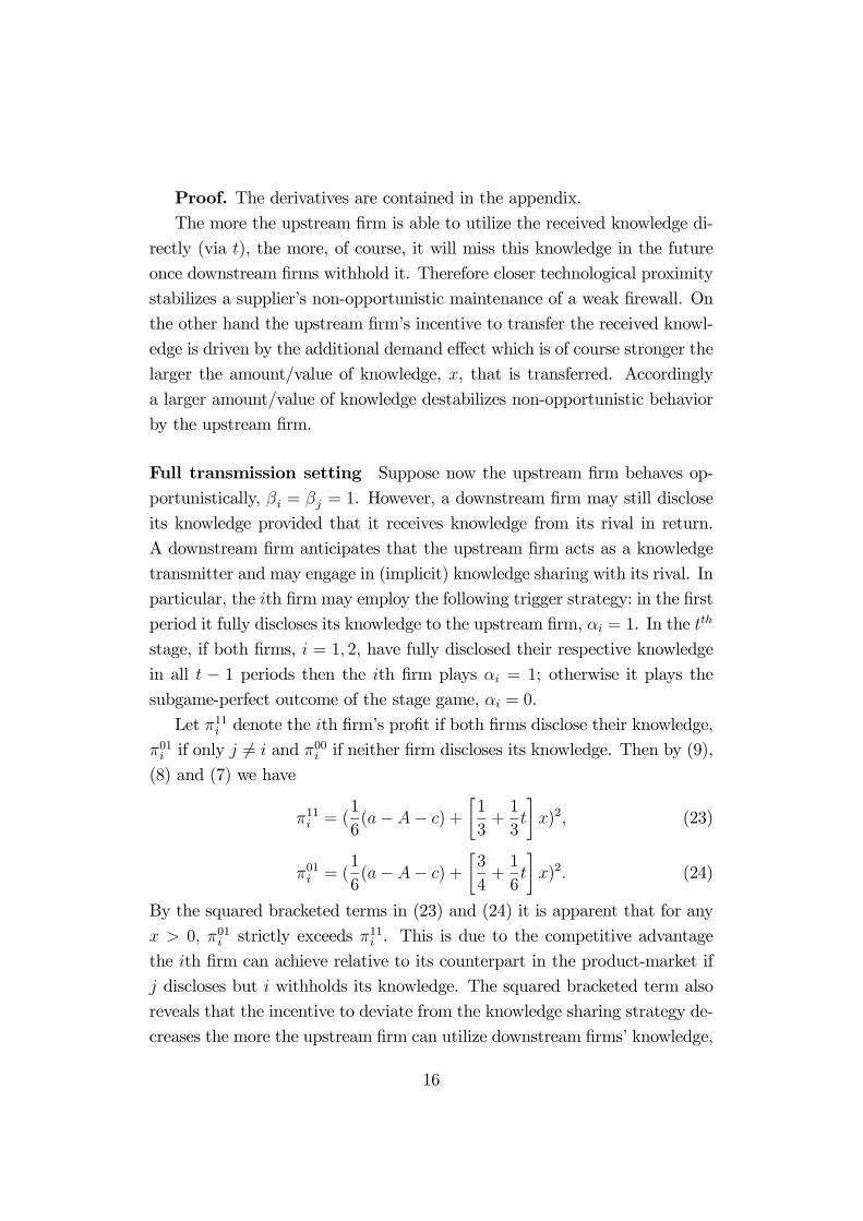
Proof. The derivatives are contained in the appendix.The more the upstream firm is able to utilize the received knowledge di-
rectly (via t), the more, of course, it will miss this knowledge in the future
once downstream firms withhold it. Therefore closer technological proximity
stabilizes a supplier’s non-opportunistic maintenance of a weak firewall. On
the other hand the upstream firm’s incentive to transfer the received knowl-
edge is driven by the additional demand effect which is of course stronger the
larger the amount/value of knowledge, x, that is transferred. Accordingly
a larger amount/value of knowledge destabilizes non-opportunistic behavior
by the upstream firm.
Full transmission setting Suppose now the upstream firm behaves op-
portunistically, βi = βj = 1. However, a downstream firm may still disclose
its knowledge provided that it receives knowledge from its rival in return.
A downstream firm anticipates that the upstream firm acts as a knowledge
transmitter and may engage in (implicit) knowledge sharing with its rival. In
particular, the ith firm may employ the following trigger strategy: in the first
period it fully discloses its knowledge to the upstream firm, αi = 1. In the tth
stage, if both firms, i = 1, 2, have fully disclosed their respective knowledge
in all t − 1 periods then the ith firm plays αi = 1; otherwise it plays the
subgame-perfect outcome of the stage game, αi = 0.
Let π11i denote the ith firm’s profit if both firms disclose their knowledge,
π01i if only j 6= i and π00i if neither firm discloses its knowledge. Then by (9),
(8) and (7) we have
π11i = (1
6(a−A− c) +
·1
3+1
3t
¸x)2, (23)
π01i = (1
6(a−A− c) +
·3
4+1
6t
¸x)2. (24)
By the squared bracketed terms in (23) and (24) it is apparent that for any
x > 0, π01i strictly exceeds π11i . This is due to the competitive advantage
the ith firm can achieve relative to its counterpart in the product-market if
j discloses but i withholds its knowledge. The squared bracketed term also
reveals that the incentive to deviate from the knowledge sharing strategy de-
creases the more the upstream firm can utilize downstream firms’ knowledge,
16

as captured by a larger t. Finally note that the downstream firms’ profits of
the one-shot non-disclosure equilibrium,
π00i = (1
6(a−A+ x))2 (25)
are clearly smaller than those given by (23) and (24). The ith firm continues
to disclose its knowledge as long as
1
1− δπ11i > π01i +
δ
1− δπ00i (26)
where the discount rate δ is defined as above. Solving (26) for δ yields the
critical discount factor to sustain the knowledge sharing equilibrium, δf :
δf >(5− 2t)(4(a−A− c) + (13 + 6t)x)
(7 + 2t)(4(a−A− c) + (11 + 2t)x).(27)
Proposition 5 Full knowledge transmission, βi = βj = 1, and repeated
downstream knowledge disclosure, αi = αj = 1, is stabilized by an increase in
the technological proximity between the downstream and the upstream firm,
∂δf/∂t < 0, and destabilized by an increase in the value/amount of knowl-
edge, ∂δf/∂x > 0.
Proof. The derivatives are contained in the appendix.The intuition behind this result is that downstream firms not only ben-
efit directly from each other’s knowledge but also due the reduction of the
intermediate input price. Of course the latter benefit occurs only to the ex-
tent to that the downstream firms’ knowledge lowers also the upstream firm’s
production costs, as captured by t. Hence technological proximity between
vertically related firms stabilizes knowledge disclosure via the cost efficiency
effect (see (7)). In contrast a larger value of the information to be shared, x,
increases the downstream firms’ incentives to achieve a short-term competi-
tive advantage more than it increases the benefit of the cost-efficiency effect.
Thus more valuable information destabilize knowledge disclosure.
Comparison of the weak firewall and the full transmission equilib-rium Which of the two equilibria is more likely to come about given that
17

their stability is ensured by (22) and (27)? We would expect the Pareto-
superior setting to be chosen by the firms. By Proposition 1 the upstream
firm will certainly prefer the full transmission setting. It remains to be val-
idated which setting appears beneficial from the downstream firms’ point
of view. We thus need to compare the downstream firms’ disclosure profits
of the full transmission setting, π11i as given by (23), with the downstream
firms’ profits in the weak firewall setting. Let π2/5i denote the latter profit,
i.e. αi = αj = 1 and βj = βi = 2/5t. Then by (9), (8) and (7) we get
π2/5i = (
1
6(a−A− c) +
·1
6+2
5t
¸x)2,
which is smaller than the profits given by (23). Thus, downstream firms
tend to fully disclose their knowledge even under ‘opportunistic’ behavior of
the supplier. Obviously, in the full transmission setting the behavior of the
supplier is not really opportunistic. In fact, each downstream firm anticipates
that it is ‘cheated’ in the same way by the common supplier as its rival.
The upstream firm acts as an intermediary that guarantees the complete
transfer of knowledge disclosed by downstream firms. Though downstream
firms could just as well engage in a direct (horizontal) exchange of knowledge,
the indirect exchange via the common supplier generates an extra benefit: it
lowers the input price if t > 0. This effect stabilizes the knowledge sharing
equilibrium and does not exist in pure horizontal knowledge sharing.
5 Summary and Conclusion
We have analyzed the conditions for knowledge disclosure in buyer-supplier
relationships. The key feature of our model is the notion of a common sup-
plier through which knowledge disclosed by one buyer may leak out to the
other one. Downstream knowledge disclosure thus bears the risk of benefit-
ting one’s rival. In such a setting the conditions for knowledge disclosure by
buyers (see Table 1, second column) are driven by the anticipated behavior
of the common supplier (third column) and the mode in which knowledge
disclosure takes place (first column).
The analysis of the one-shot relationship setting provides the following
results:
18

Knowledge disclosure modeBuyers’
knowledge
disclosure, α∗
Supplier’s
knowledge
transmission, β∗
One-shot relationship
absence of
supplier opportunism∗100%⇔ β < 40%
0%⇔ β > 40%exogenous
presence of
supplier opportunism0% 100%
buyer-supplier cooperation 100% 100%
reciprocal exchange 0% 100%
Repeated relationships
weak firewall∗ 100% 40%
full transmission 100% 100%∗ The displayed results imply t=1, for details see Lemma 1 and section 4.
Table 1: Equilibrium solutions of the game’s first stage (buyers’ knowledge
disclosure) and second stage (supplier’s knowledge transmission) respectively
If the downstream firm is confident that the common upstream supplier does
not transmit ‘too much’ of the disclosed knowledge to its competitor, full
knowledge disclosure occurs even if the competitor benefits more from this
than the disclosing firm itself. In contrast, downstream knowledge disclo-
sure will not occur at all if buyers anticipate opportunistic behavior of their
common supplier. In fact the supplier’s announcement to treat the obtained
knowledge confidentially (to install a firewall) is not credible in a one-shot
relationship.
One way to overcome this knowledge sharing dilemma is buyer-supplier
cooperation (i.e. joint profit maximization). The upstream firm can compen-
sate the downstream firm for its losses, as the supplier’s gain from knowledge
disclosure is higher than the buyer’s loss. On the other hand, reciprocal
knowledge exchange does not facilitate knowledge disclosure by downstream
firms. The upstream firm’s announcement to hold back its own knowledge
as a response of refused downstream knowledge disclosure is not credible.
In the case of repeated relationships we identify two possible equilibria:
19

In the first one buyers proceed with complete knowledge disclosure as long
as the supplier maintains a weak firewall. In the second, more subtle one,
knowledge disclosure occurs even under full knowledge transmission through
the supplier. Here the supplier acts as an intermediary for implicit down-
stream knowledge sharing. Both the weak firewall and the full transmission
setting are stabilized by an increase in the degree of technological proximity
between the downstream and the upstream firm whereas they are destabi-
lized by an increase in the value/amount of knowledge. The latter suggests
that a downstream firm’s disclosure of incremental innovations is more likely
than disclosure of major innovations.
As a by-product we provide an additional explanation for intraindustry
knowledge spillovers. These are usually regarded as an involuntary leakage of
knowledge. According to our results intraindustry spillovers may well be the
result of voluntary knowledge disclosure to suppliers and further knowledge
transmission respectively. A higher degree of technological proximity be-
tween customers and suppliers facilitates voluntary inter industry knowledge
spillovers as well as intraindustry spillovers.
Our model has several possible extensions. One can analyze, for instance,
how product differentiation affects downstream firms’ incentives for knowl-
edge disclosure. In our model firms in the downstream industry make use
of one input to produce a homogenous final product. This implies that all
firms in the downstream industry benefit from lower input prices due to
knowledge disclosure in the same way. Suppose that firms in the down-
stream industry offer differentiated products and that specific intermediate
inputs are required to produce them. Then, it is not guaranteed that knowl-
edge disclosure by one downstream firm leads to identical price reductions
for all intermediate inputs. Moreover, varying degrees of competition in the
upstream and the downstream industry may also influence the results. Fur-
thermore, our model with symmetric downstream firms can be extended to
one with asymmetric firms which differ, for instance, with respect to their
ability to make use of the rival’s knowledge.
Acknowledgements We would like to thank Stefan Napel and Wil-
helm Pfähler for very helpful comments.
20

Appendix
Proposition 4 By (22) we calculate
∂δw∂t
= − 24(10((a−A)2 + c2) + f1 + f2 + f3)
(25(1 + 2t)2(2(a−A− c) + (3 + 2t)x))2< 0,
where
f1 = (a−A)(25 + 24t+ 4t2)x > 0,f2 = (15 + 36t+ 28t2)x2 > 0,f3 = (20(a−A) + (25 + 24t+ 4t2)x)c > 0,
and∂δw∂x
=24t(5− 2t)(a−A− c)
(25(1 + 2t)(2(a−A− c) + (3 + 2t)x))2> 0.
Proposition 5 By (27) we have
∂δf∂t
= −16(24((a−A)2 + c2) + g1 + g2 + g3)
(7 + 2t)(4(a−A− c) + (11 + 2t)x)2< 0,
with
g1 = (a−A)(109 + 52t+ 4t2)x > 0,g2 = (127 + 148t+ 28t2)x2 > 0,g3 = (48(a−A) + (109 + 52t+ 4t2)x)c > 0.
Finally note that
∂δf∂x
=8(5 + 8t− 4t2)(a−A− c)
(7 + 2t)(4(a−A− c) + (11 + 2t)x)2> 0.
21
References
[1] Abreu, D.J. (1986). Extremal equilibria of oligopolistic supergames.
Journal of Economic Theory, 39, 191-225.
[2] Abreu. D.J. (1988). On the theory of infinitely repeated games with
discounting. Econometrica, 56, 383-396.
[3] Appleyard, M. (1996). How Does Knowledge Flow? Interfirm Patterns
in the Semiconductor Industry. Strategic Management Journal, 17, 137-
154.
[4] Atallah, G. (2002). Vertical R&D Spillovers, Cooperations, Market
Structure, and Innovation. Economics of Innovation and New Technol-
ogy, 11, 179-202.
[5] Atallah, G. (2003). Information Sharing and the Stability of Cooper-
ation in Research Joint Ventures. Economics of Innovation and New
Technology, 12, 531-554.
[6] Baiman, S., Rajan, M.V. (2002). The Role of Information and Oppor-
tunism in the Choice of Buyer-Supplier Relationships. Journal of Ac-
counting Research, 40, 247-278.
[7] Bönte, W. (2005). Inter-Firm Trust in Buyer-Supplier Relations: Are
Knowledge Spillovers and Geographical Proximity Relevant? Working
Paper, University of Hamburg.
[8] Bönte, W., Keilbach, M. (2005). Concubinage or Marriage? Informal
and Formal Cooperations for Innovation. International Journal of In-
dustrial Organization, 23 , 279-302.
[9] Banerjee, S., Lin P. (2003). Downstream R&D, raising rival’s costs, and
input price contracts. International Journal of Industrial Organization,
21, 79-97.
[10] Cassiman, B., Veugelers, R. (2002). R&d Cooperation and Spillovers:
Some Empirical Evidence from Belgium. American Economic Review,
92, 1169-1184.
22

[11] D’Aspremont, C. and Jacquemin, A. (1988). Cooperative and noncoop-
erative R&D in duopoly with spillovers. American Economic Review,
78, 1133-1137.
[12] Dyer, J.H., Hatch, N.W. (2004 a). Using Supplier Networks to Learn
Faster. MIT Sloan Management Review, 45, 3, 57-64.
[13] Dyer, J.H., Hatch, N.W. (2004 b). Network-specific capabilities, network
barriers to knowledge transfers, and competitive advantage. Academy of
Management Proceedings, V1-V6.
[14] Grindley, P., Mowery, D. and Silverman, B. (1994). SEMATECH and
collaborative research: Lessons for the design of high technology consor-
tia. Journal of Policy Analysis and Management, 13, 723-758.
[15] Harabi, N. (1998). Innovation through Vertical Relations between Firms,
Suppliers and Customers: a Study of German Firms. Industry and In-
novation, 5, 157-179.
[16] Harhoff, D. (1996). Strategic Spillovers and Incentives for Research and
Development. Management Science, 42, 907-925.
[17] Harhoff, D., Henkel, J., von Hippel, E. (2003). Profiting from volun-
tary information spillovers: how users benefit by freely revealing their
innovations. Research Policy 32, 1753-1769.
[18] Ishii, A. (2004). Cooperative R&D between vertically related firms with
spillovers. International Journal of Industrial Organization, 22, 1213-
1226.
[19] Jost, P.-J. (2005). The Limits of Networking: The Case of R&D-
Cooperations. Discussion Paper Series in Economics and Management
(GEABA), No. 05-10.
[20] Kamien, M., Muller, E., Zang, I. (1992). Research Joint Ventures and
R&D Cartels. American Economic Review, 82, 1293-1306.
23

[21] Kamien, M., Zang, I. (2000). Meet me halfway: research joint ventures
and absorptive capacity. International Journal of Industrial Organiza-
tion, 18, 995-1012.
[22] Kotabe, M., Martin, X., Domoto, H. (2003). Gaining from vertical
partnerships: Knowledge transfer, relationship duration, and supplier
performance in the U.S. and Japanese automotive industries. Strategic
Management Journal, 24, 293-316.
[23] Kultti, K. and Takalo, T. (1998). R&D spillovers and information ex-
change. Economics Letters, 61, 121-123.
[24] Lee, H.L., So, K.C., Tang, C.S. (2000). The value of information sharing
in a two-level supply chain. Management Science 46, 626-643.
[25] Lee, H.L., Whang, S. (2000). Information sharing in a supply chain.
International Journal of Technology Management, 20, 373-387.
[26] Li, L. (2002). Information Sharing in a Supply Chain with Horizontal
Competition. Management Science, 48, 1196-1212.
[27] Milliou, C. (2004). Vertical Integration and R&D information flow: is
there a need for ‘firewalls’? International Journal of Industrial Organi-
zation, 22, 25-34.
[28] Sattler, H., Schrader, S. and Lüthje, C. (2003). Informal cooperation in
the US and Germany: cooperative managerial capitalism in interfirm
information trading. International Business Review, 12, 273-295.
[29] Schrader, S., (1990). Informal technology transfer between firms: Coop-
eration through information trading. Research Policy, 20, 153-170.
[30] Wiethaus, L. (2005). Absorptive Capacity and Connectedness: Why
competing firms also adopt identical R&D approaches. International
Journal of Industrial Organization, 23, 467-481.
[31] Zhang, H. (2002). Vertical Information Exchange in a Supply Chain
with Duopoly Retailers. Production and Operations Management 11,
531-546.
24


Curriculum Vitae
Date/Place of Birth: 29 January 1975 in Herdecke
Education
o Doctoral Studies in Economics, University of Hamburg, July
2002 – November 2005
o Diploma in Business Administration, University of Hamburg, May 2002
o Independent Studies, University of Notre Dame, September
2001 – January 2002
o Abitur, Gymnasium Wildeshausen, 1994
Professional Experience
o Research and Teaching Fellow (Wissenschaftlicher Mitar-
beiter), University of Hamburg, September 2002 – August 2005
o Freelancer, Q & A Qualified Analysis (Consulting), Hamburg,
September 2004 – January 2005
o Intern, DGM Consulting (Deutsche Gesellschaft für Mittelstandsberatung), Hamburg, October 1999 – December 1999
o Intern, Haspa (Hamburger Sparkasse), August 1998 – April 1999
o Intern, RITZ Messwandler, Hamburg, July 1998 – September 1998