Embed Size (px)
Citation preview

Business and Economics
It is the fun It is the reality
It is the true leader of the world

"People shouldn't bury themselves in the mathematics, because the mathematics are only tools," says Kenneth Froot, a professor at Harvard Business School who teaches courses in risk management. "One needs to have a wide and robust vocabulary to talk about risk, simply because no single mathematical formula is going to capture all of what risk is."

Copyright © 2007 Pearson Addison-Wesley. All rights reserved.
3-3
Meaning of Money
• Money (money supply)—anything that is generally accepted in payment for goods or services or in the repayment of debts;
• Wealth—the total collection of pieces of property that serve to store value
• Income—flow of earnings per unit of time

Copyright © 2007 Pearson Addison-Wesley. All rights reserved.
3-4
Evolution of the Payments System
• Commodity Money ( Gold Standard & Breton Wood) • Fiat Money• Checks• Electronic Payment• E-Money
Copyright © 2007 Pearson Addison-Wesley. All rights reserved.
3-5
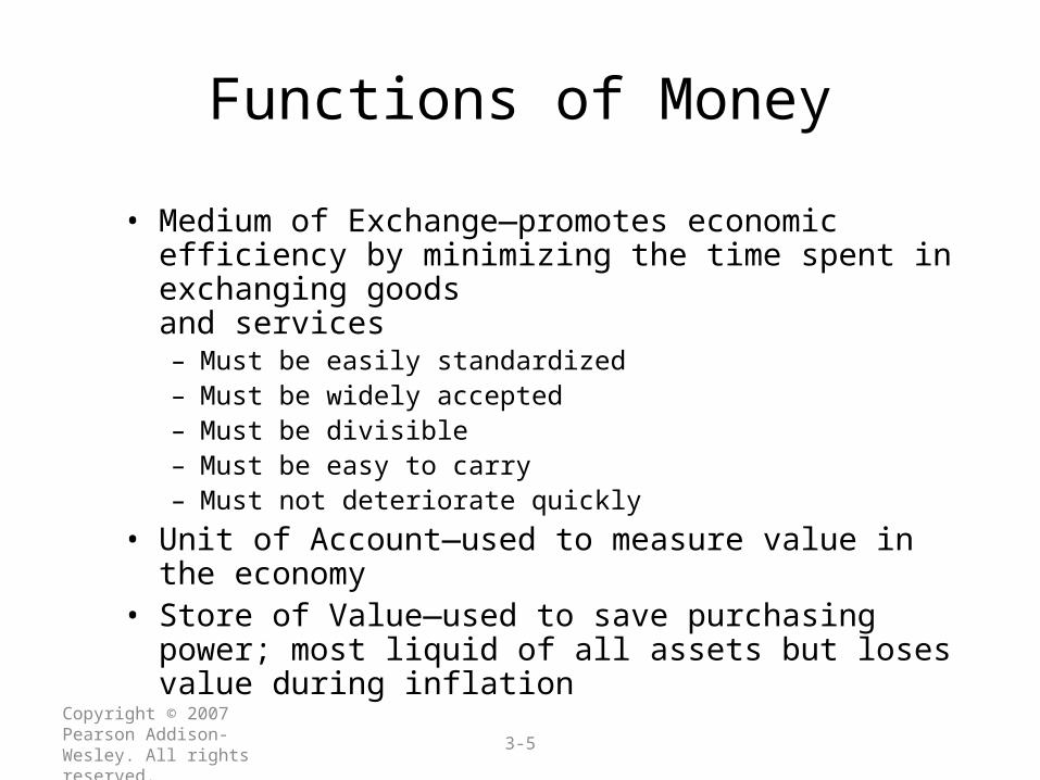
Functions of Money
• Medium of Exchange—promotes economic efficiency by minimizing the time spent in exchanging goods and services– Must be easily standardized– Must be widely accepted– Must be divisible– Must be easy to carry– Must not deteriorate quickly
• Unit of Account—used to measure value in the economy
• Store of Value—used to save purchasing power; most liquid of all assets but loses value during inflation
0
100
200
300
400
500
600
700
1850 1875 1900 1925 1950 1975 2000
GOLDPRICE
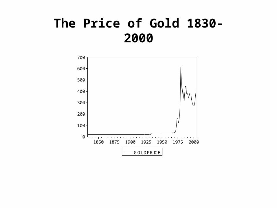
The Price of Gold 1830-2000
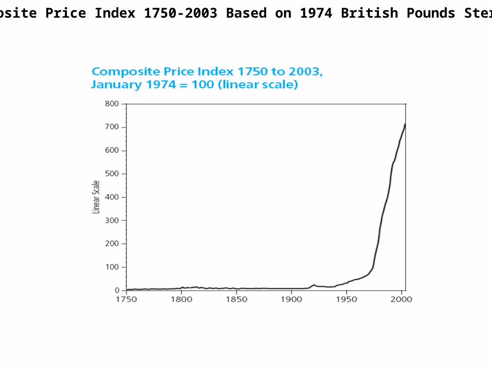
Composite Price Index 1750-2003 Based on 1974 British Pounds Sterling

US Gold Reserves between 1944 and 2004 (millions of ounces)

Purchasing Power of the Currencies of the Ten Leading Industrial Nations from 1980-1999 (in 1980 adjusted values)
0.00%
20.00%
40.00%
60.00%
80.00%
100.00%
120.00%
1980 1981 1982 1983 1984 1985 1986 1987 1988 1989 1990 1991 1992 1993 1994 1995 1996 1997 1998
اليابان
ألمانيا
سويسرا
النمسا
أمريكا
فرنسا
كندا
بريطانيا
أسبانيا
إيطاليا
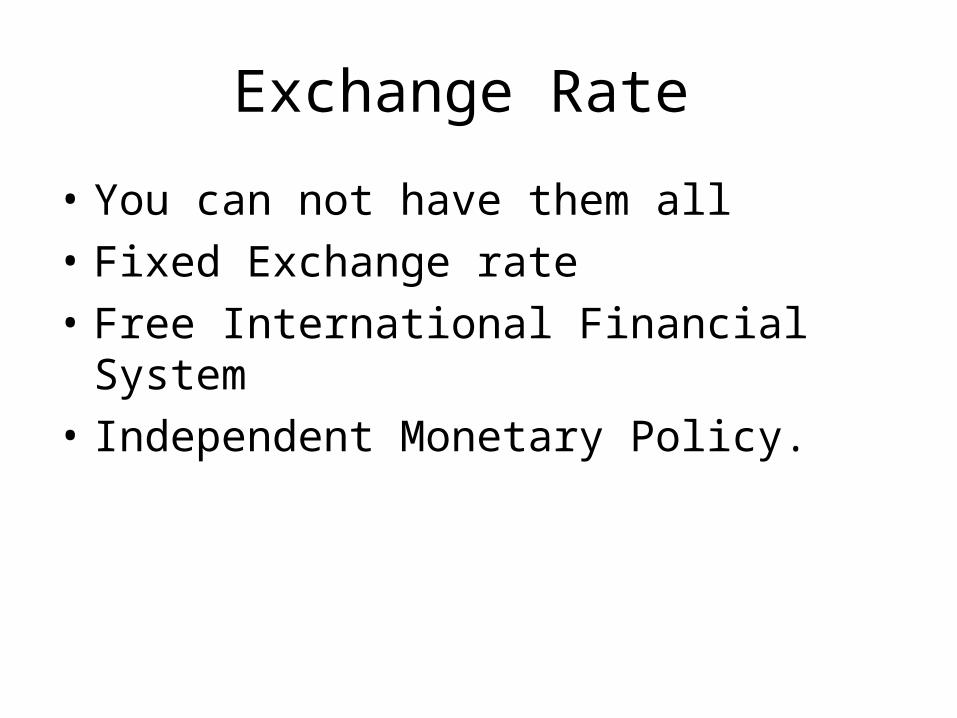
Exchange Rate
• You can not have them all• Fixed Exchange rate • Free International Financial System• Independent Monetary Policy.

The Business CycleLe
vel o
f Rea
l Out
put
Time
Peak
Peak
Peak
Recession
Recession
Expa
nsio
n Expa
nsio
n
Trough
Trough
Growth
Trend
O 7.1Phases of the Business Cycle

Copyright © 2007 Pearson Addison-Wesley. All rights reserved.
1-12
Money and Business Cycles
• Evidence suggests that money plays an important role in generating business cycles
• Recessions (unemployment) and booms (inflation) affect all of us
• Monetary Theory ties changes in the money supply to changes in aggregate economic activity and the price level

English Price Level and Real Wage, 1264-2002 (1270 = 100)

Consumer Prices in the United States,1776-2003

Inflation Has Remained Low and Stable in Recent Years

Money and Hyperinflation in Germany, 1922-1924

The Evolving U.S. Economy
– Figure interprets the changes in real GDP and the price level each year from 1960 to 2005 in terms of shifting AD, SAS, and LAS curves.
– In 1960, the price level was 21 and real GDP was $2.5 trillion.
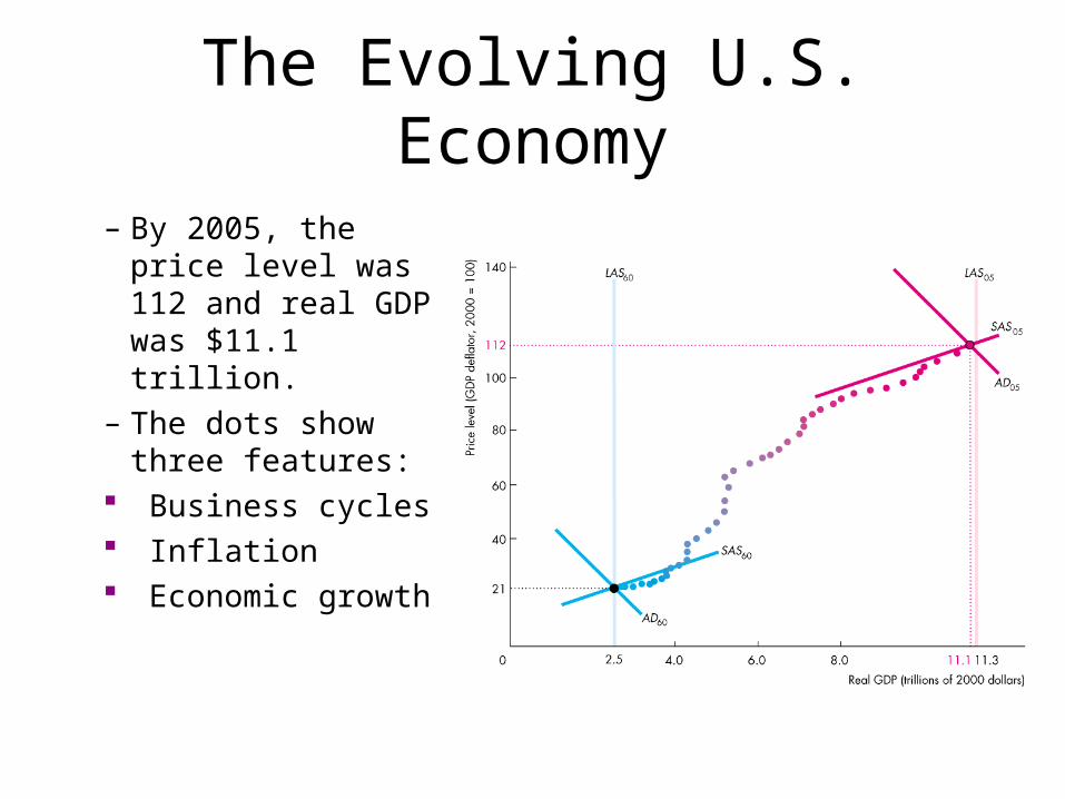
The Evolving U.S. Economy
– By 2005, the price level was 112 and real GDP was $11.1 trillion.
– The dots show three features:
Business cycles Inflation Economic growth
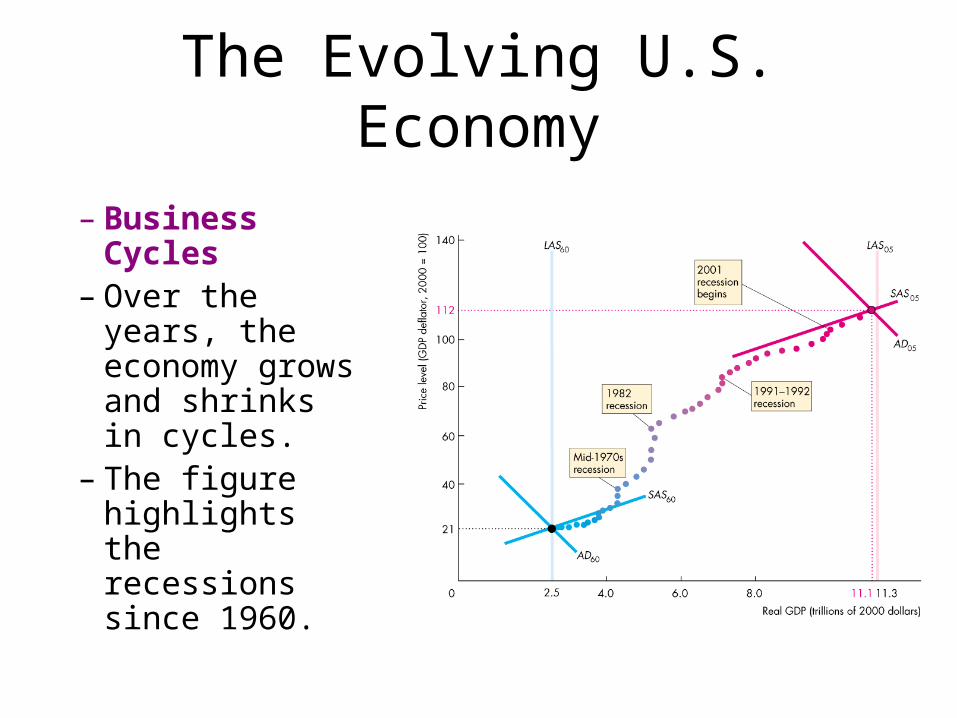
The Evolving U.S. Economy
– Business Cycles– Over the years,
the economy grows and shrinks in cycles.
– The figure highlights the recessions since 1960.

The Evolving U.S. Economy
– Inflation– The upward
movement of the dots shows inflation.
– Economic Growth– The rightward
movement of the dots shows the growth of real GDP.

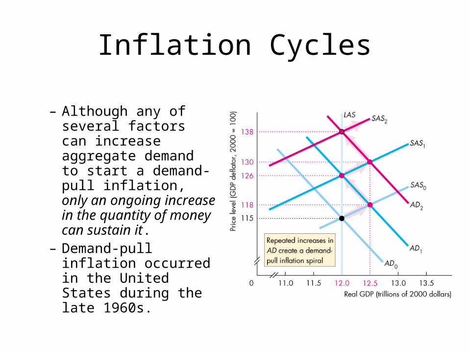
Inflation Cycles
– In the long run, inflation occurs if the quantity of money grows faster than potential GDP.
– In the short run, many factors can start an inflation, and real GDP and the price level interact.
– To study these interactions, we distinguish two sources of inflation:
Demand-pull inflation Cost-push inflation

Inflation Cycles
– Demand-Pull Inflation– An inflation that starts because aggregate demand
increases is called demand-pull inflation. – Demand-pull inflation can begin with any factor
that increases aggregate demand. – Examples are a cut in the interest rate, an increase
in the quantity of money, an increase in government expenditure, a tax cut, an increase in exports, or an increase in investment stimulated by an increase in expected future profits.

Inflation Cycles
• Initial Effect of an Increase in Aggregate Demand– Figure (a) illustrates
the start of a demand-pull inflation.
– Starting from full employment, an increase in aggregate demand shifts the AD curve rightward.

Inflation Cycles
– The price level rises, real GDP increases, and an inflationary gap arises.
– The rising price level is the first step in the demand-pull inflation.

Inflation Cycles
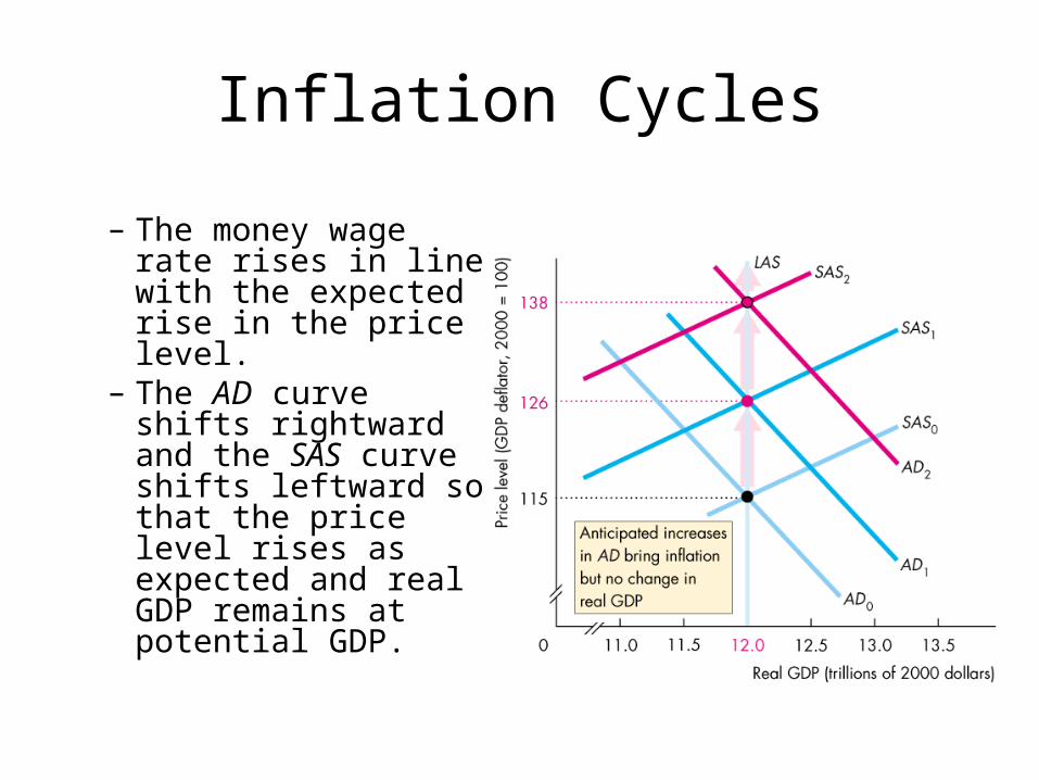
• Money Wage Rate Response– Figure (b) illustrates the
money wage response. – The money wages rises
and the SAS curve shifts leftward.
Real GDP decreases back to potential GDP but the price level rises further.

Inflation Cycles
• A Demand-Pull Inflation Process– Figure illustrates a
demand-pull inflation spiral.
Aggregate demand keeps increasing and the process just described repeats indefinitely.
Inflation Cycles
– Although any of several factors can increase aggregate demand to start a demand-pull inflation, only an ongoing increase in the quantity of money can sustain it.
– Demand-pull inflation occurred in the United States during the late 1960s.
Inflation Cycles
– Cost-Push Inflation– An inflation that starts with an increase in costs is
called cost-push inflation.– There are two main sources of increased costs:– 1. An increase in the money wage rate– 2. An increase in the money price of raw
materials, such as oil

Inflation Cycles• Initial Effect of a Decrease
in Aggregate Supply– Figure illustrates the start
of cost-push inflation.– A rise in the price of oil
decreases short-run aggregate supply and shifts the SAS curve leftward.
– Real GDP decreases and the price level rises.

Inflation Cycles
• Aggregate Demand Response– The initial increase in costs creates a one-time rise in
the price level, not inflation.– To create inflation, aggregate demand must increase. – That is, the Fed must increase the quantity of money
persistently.

Inflation Cycles
– Figure illustrates an aggregate demand response.
– Suppose that the Fed stimulates aggregate demand to counter the higher unemployment rate and lower level of real GDP.
– Real GDP increases and the price level rises again.

Inflation Cycles
• A Cost-Push Inflation Process– If the oil producers
raise the price of oil to try to keep its relative price higher,
– and the Fed responds by increasing the quantity of money,
– a process of cost-push inflation continues.
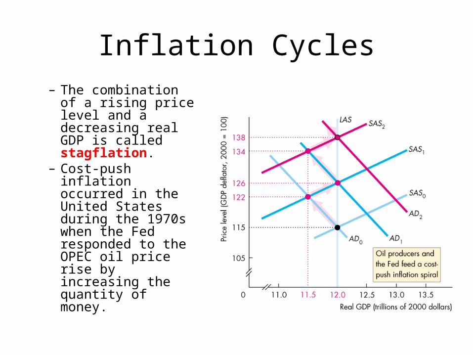
Inflation Cycles– The combination of
a rising price level and a decreasing real GDP is called stagflation.
– Cost-push inflation occurred in the United States during the 1970s when the Fed responded to the OPEC oil price rise by increasing the quantity of money.
Inflation Cycles
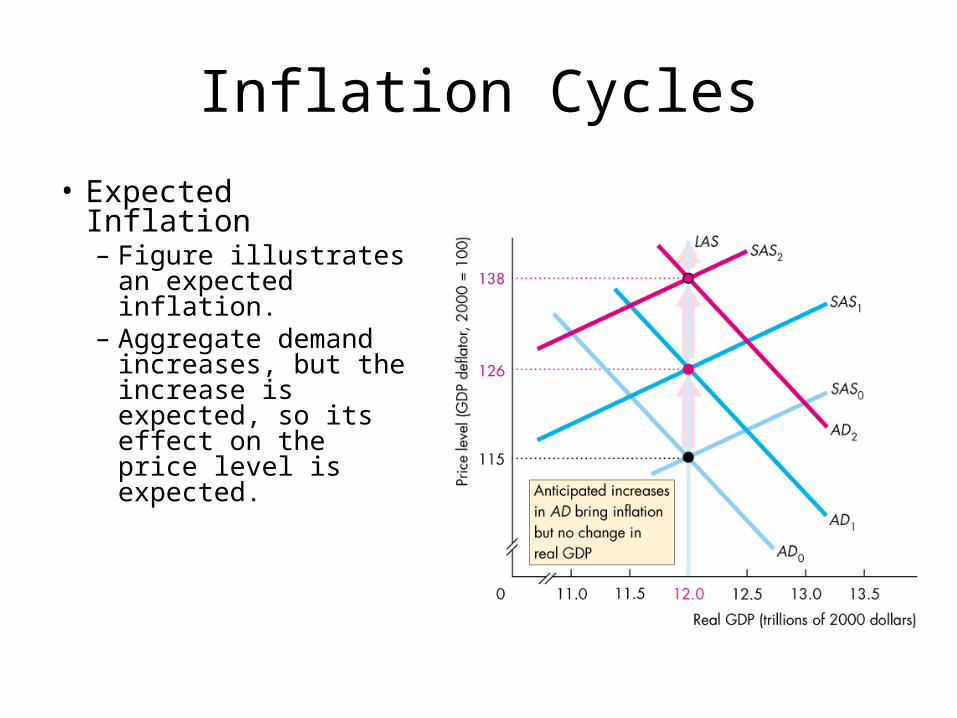
• Expected Inflation– Figure illustrates an
expected inflation.– Aggregate demand
increases, but the increase is expected, so its effect on the price level is expected.
Inflation Cycles
– The money wage rate rises in line with the expected rise in the price level.
– The AD curve shifts rightward and the SAS curve shifts leftward so that the price level rises as expected and real GDP remains at potential GDP.

Inflation Cycles
• Forecasting Inflation– To expect inflation, people must forecast it.– The best forecast available is one that is based on
all the relevant information and is called a rational expectation.
– A rational expectation is not necessarily correct but it is the best available.
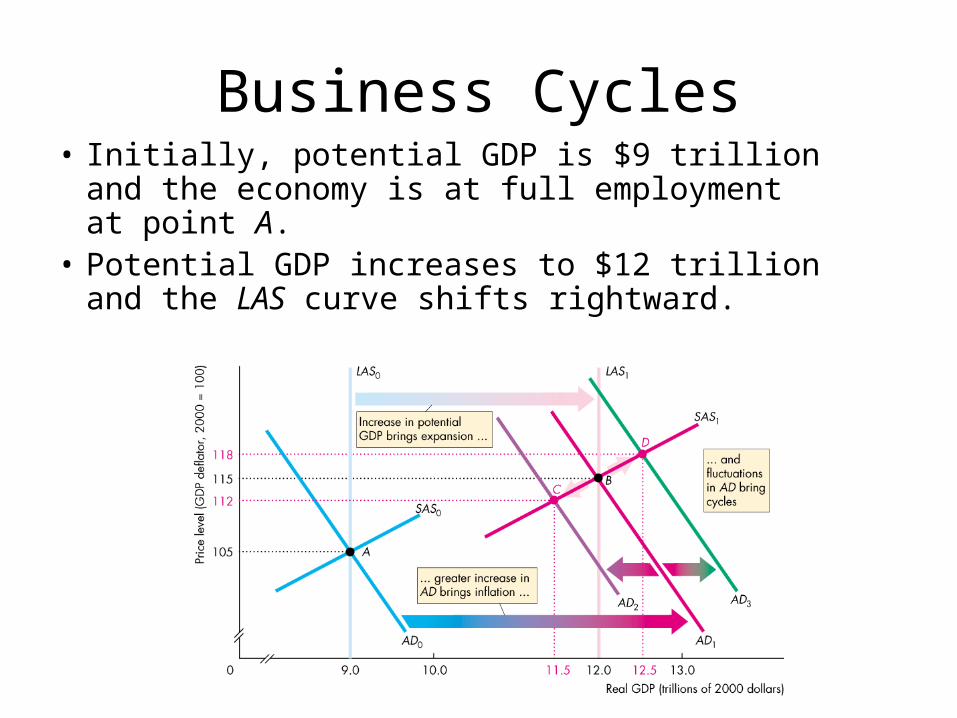
Business Cycles• Initially, potential GDP is $9 trillion and the
economy is at full employment at point A.• Potential GDP increases to $12 trillion and
the LAS curve shifts rightward.
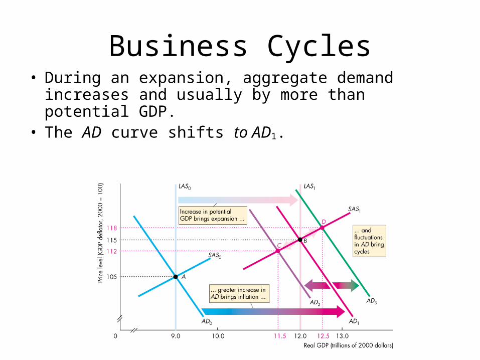
Business Cycles• During an expansion, aggregate demand increases
and usually by more than potential GDP.• The AD curve shifts to AD1.

Business Cycles• Assume that during this expansion the price level
is expected to rise to 115 and that the money wage rate was set on that expectation.
• The SAS shifts to SAS1.
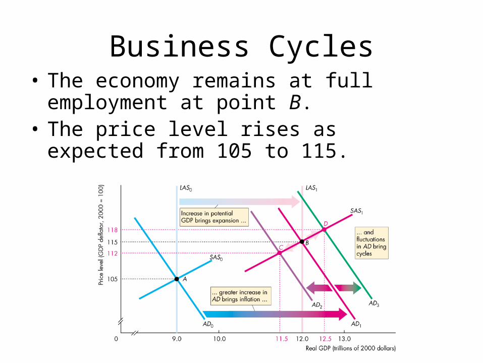
Business Cycles• The economy remains at full employment at
point B.• The price level rises as expected from 105 to
115.

Business Cycles• But if aggregate demand increases more slowly
than potential GDP, the AD curve shifts to AD2.• The economy moves to point C.• Real GDP growth is slower and inflation is less
than expected.

Business Cycles• But if aggregate demand increases more quickly
than potential GDP, the AD curve shifts to AD2.• The economy moves to point D.• Real GDP growth is faster and inflation is higher
than expected.
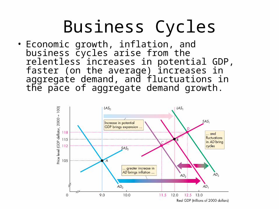
Business Cycles• Economic growth, inflation, and business cycles
arise from the relentless increases in potential GDP, faster (on the average) increases in aggregate demand, and fluctuations in the pace of aggregate demand growth.
The Federal Budget
– The federal budget is the annual statement of the federal government’s outlays and tax revenues.
– The federal budget has two purposes:– 1. To finance the activities of the federal government– 2. To achieve macroeconomic objectives– Fiscal policy is the use of the federal budget to
achieve macroeconomic objectives, such as full employment, sustained economic growth, and price level stability.
The Supply-Side: Employment and Potential GDP
– Fiscal policy has important effects employment, potential GDP, and aggregate supply—called supply-side effects.
– An income tax changes full employment and potential GDP.
The Supply-Side: Employment and Potential GDP
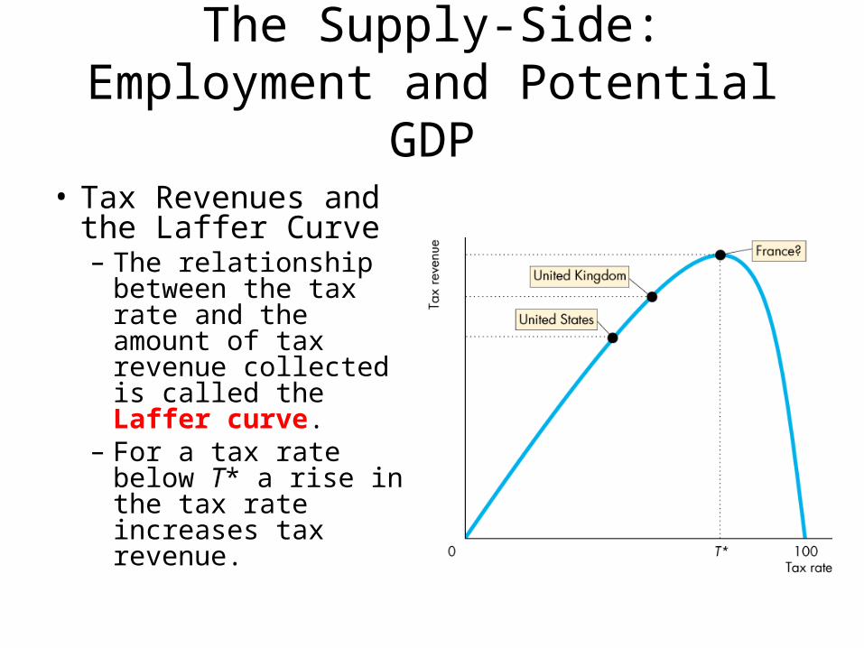
• Tax Revenues and the Laffer Curve – The relationship
between the tax rate and the amount of tax revenue collected is called the Laffer curve.
– For a tax rate below T* a rise in the tax rate increases tax revenue.

The Conduct of Monetary Policy
• The Federal Funds Rate– The Fed’s choice of policy instrument (which is the
same choice as that made by most other major central banks) is a short-term interest rate.
– Given this choice, the exchange rate and the quantity of money find their own equilibrium values.
– The specific interest rate that the Fed targets is the federal funds rate, which is the interest rate on overnight loans that banks make to each other.

The Conduct of Monetary Policy
• Hitting the Federal Funds Rate Target: Open Market Operations– An open market operation is the purchase or sale of
government securities by the Fed from or to a commercial bank or the public.
– When the Fed buys securities, it pays for them with newly created reserves held by the banks.
– When the Fed sells securities, they are paid for with reserves held by banks.
– So open market operations influence banks’ reserves.
Origins and Issues of Macroeconomics
– Economists began to study economic growth, inflation, and international payments during the 1750s.
– Modern macroeconomics dates from the Great Depression, a decade (1929-1939) of high unemployment and stagnant production throughout the world economy.
– John Maynard Keynes book, The General Theory of Employment, Interest, and Money, began the subject.
Origins and Issues of Macroeconomics
• Short-Term Versus Long-Term Goals– Keynes focused on the short-term—on
unemployment and lost production.– “In the long run,” said Keynes, “we’re all dead.”– During the 1970s and 1980s, macroeconomists
became more concerned about the long-term—inflation and economic growth.

Economic Growth and Fluctuations
–Economic growth is the expansion of the economy’s production possibilities—an outward shifting PPF.–We measure economic growth by the increase in real GDP.–Real GDP (real gross domestic product) is the value of the total production of all the nation’s farms, factories, shops, and offices, measured in the prices of a single year.
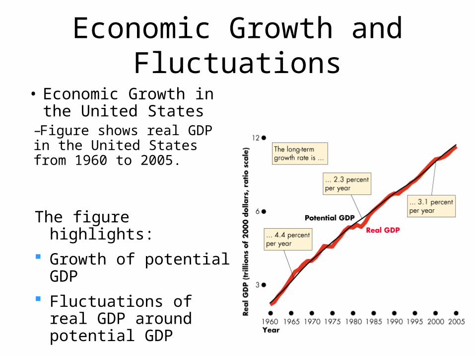
Economic Growth and Fluctuations
• Economic Growth in the United States–Figure shows real GDP in the United States from 1960 to 2005.
The figure highlights: Growth of potential GDP Fluctuations of real GDP
around potential GDP

Economic Growth and Fluctuations
–Growth of Potential GDP–Potential GDP is the value of production when all the economy’s labor, capital, land, and entrepreneurial ability are fully employed.–During the 1970s, the growth of output per person slowed—a phenomenon called the productivity growth slowdown.
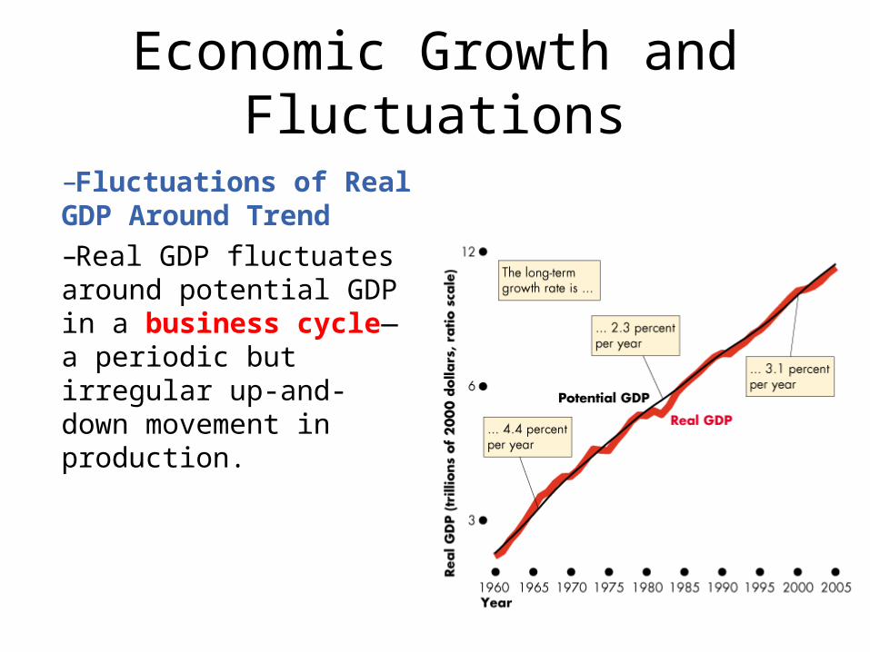
Economic Growth and Fluctuations
–Fluctuations of Real GDP Around Trend–Real GDP fluctuates around potential GDP in a business cycle—a periodic but irregular up-and-down movement in production.

Economic Growth and Fluctuations
–Every business cycle has two phases:–1. A recession–2. An expansion–and two turning points:–1. A peak–2. A trough–Figure on the next slide illustrates these features of the business cycle.

Economic Growth and Fluctuations– Most recent business cycle in the United States

Economic Growth and Fluctuations
–A recession is a period during which real GDP decreases for at least two successive quarters.–An expansion is a period during which real GDP increases.
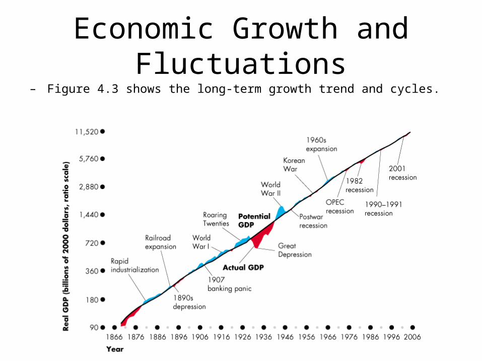
Economic Growth and Fluctuations– Figure 4.3 shows the long-term growth trend and cycles.
Economic Growth and Fluctuations
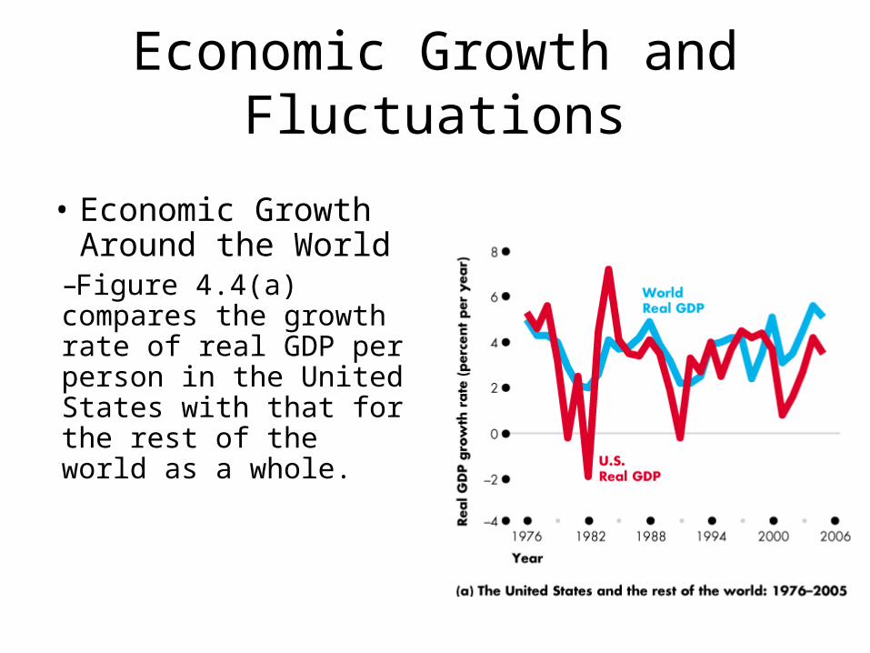
• Economic Growth Around the World–Figure 4.4(a) compares the growth rate of real GDP per person in the United States with that for the rest of the world as a whole.
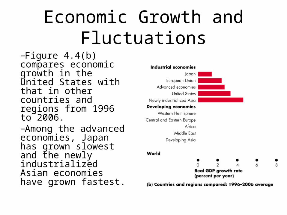
Economic Growth and Fluctuations–Figure 4.4(b) compares economic growth in the United States with that in other countries and regions from 1996 to 2006.–Among the advanced economies, Japan has grown slowest and the newly industrialized Asian economies have grown fastest.
Economic Growth and Fluctuations
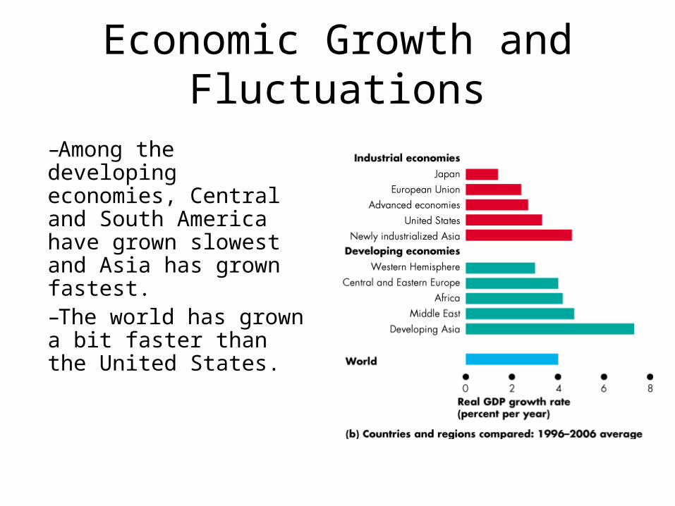
–Among the developing economies, Central and South America have grown slowest and Asia has grown fastest.–The world has grown a bit faster than the United States.

• The Lucas Wedge and Okun Gap– How costly are the growth slowdown and the
lost output over the business cycle?– To answer that question we measure: The Lucas wedge The Okun gap
Economic Growth and Fluctuations

• The Lucas Wedge– The Lucas wedge is
the accumulated loss of output from the productivity growth slowdown of the 1970s .
– Figure 4.5(a) shows that the Lucas wedge is $72 trillion or 6.5 times the real GDP in 2005.
Economic Growth and Fluctuations
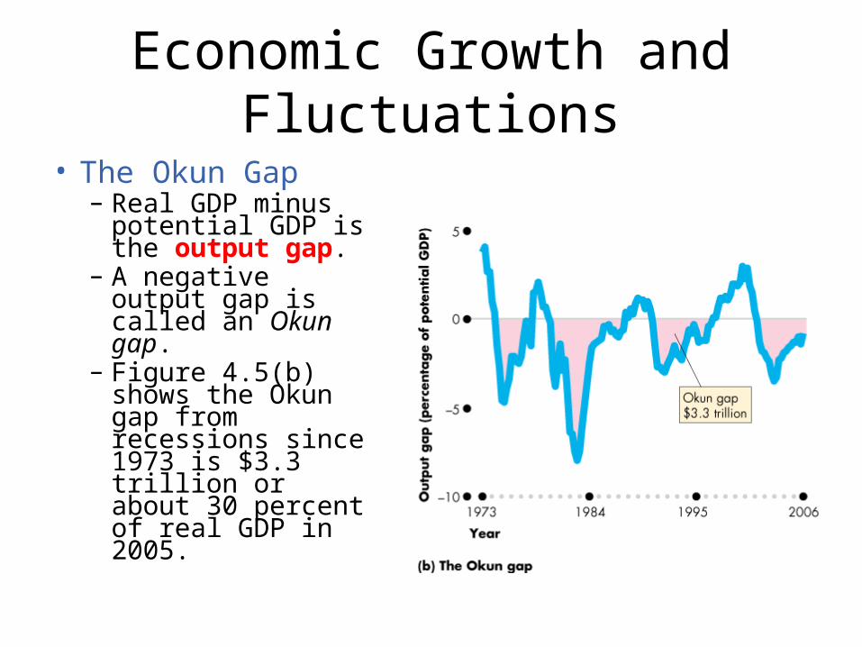
• The Okun Gap– Real GDP minus
potential GDP is the output gap.
– A negative output gap is called an Okun gap.
– Figure 4.5(b) shows the Okun gap from recessions since 1973 is $3.3 trillion or about 30 percent of real GDP in 2005.
Economic Growth and Fluctuations
• Benefits and Costs of Economic Growth– The Lucas wedge is a measure of the dollar value of
lost real GDP if the growth rate slows. This cost translates into real goods and services.
– It is a cost in terms of less health care for the poor and elderly, less cancer and AIDS research, worse roads, and less to spend on clean air, more trees, and cleaner lakes.
– But fast growth is also costly. Its main costs is forgone current consumption. To sustain growth, resources must be allocated to advancing technology and accumulating capital rather than to current consumption.
Economic Growth and Fluctuations
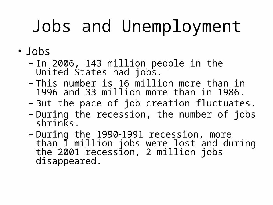
Jobs and Unemployment• Jobs– In 2006, 143 million people in the United States
had jobs.– This number is 16 million more than in 1996 and
33 million more than in 1986. – But the pace of job creation fluctuates.– During the recession, the number of jobs shrinks.– During the 19901991 recession, more than 1
million jobs were lost and during the 2001 recession, 2 million jobs disappeared.

Jobs and Unemployment• Unemployment– Not everyone who wants a job can find one. – On an average day in a normal year, 7 million
people in the United States are unemployed.– In a recession, the number is larger. For example,
in 1990-1991 recession, 9 million people were looking for jobs.
– The unemployment rate is the number of unemployed people expressed as a percentage of all the people who have jobs or are looking for one.

Jobs and Unemployment– The unemployment rate is not a perfect measure of
the underutilization of labor. For two reasons:– The unemployment rate – 1. Excludes people who are so discouraged that
they have given up looking for jobs.– 2. Measures unemployed people rather than
unemployed labor hours. So it does not tells us about the number of part-time workers who want full-time jobs.

Jobs and Unemployment• Unemployment in in United States– Figure 4.6 shows the unemployment rate from
1926 to 2006.

Jobs and Unemployment– During the 1930s, the unemployment rate hit 25 percent.
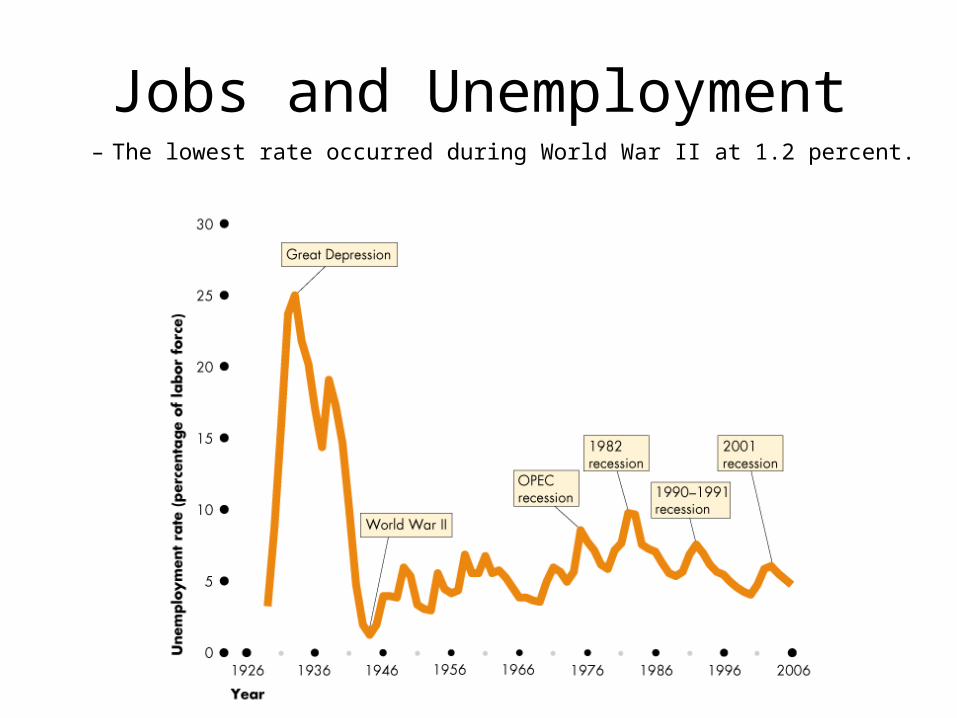
Jobs and Unemployment– The lowest rate occurred during World War II at 1.2 percent.

Jobs and UnemploymentDuring recent recessions, the unemployment rate increased but was not as high as in the Great Depression.

Jobs and UnemploymentThe unemployment rate is never zero. Since World War II, it has averaged 5 percent.

Jobs and Unemployment• Unemployment
Around the World– Figure 4.7 compares
the unemployment rate in the United States with those in Japan, Western Europe, and Canada.
– The U.S. unemployment rate has been lower than that in Western Europe and Canada but higher than that in Japan.

Jobs and Unemployment– The cycle in
unemployment in Canada is similar to that in the United States.
– The cycle in unemployment in Western European is out of phase with that in the United States.
– Unemployment in Japan has drifted upwards since the mid-1990s.
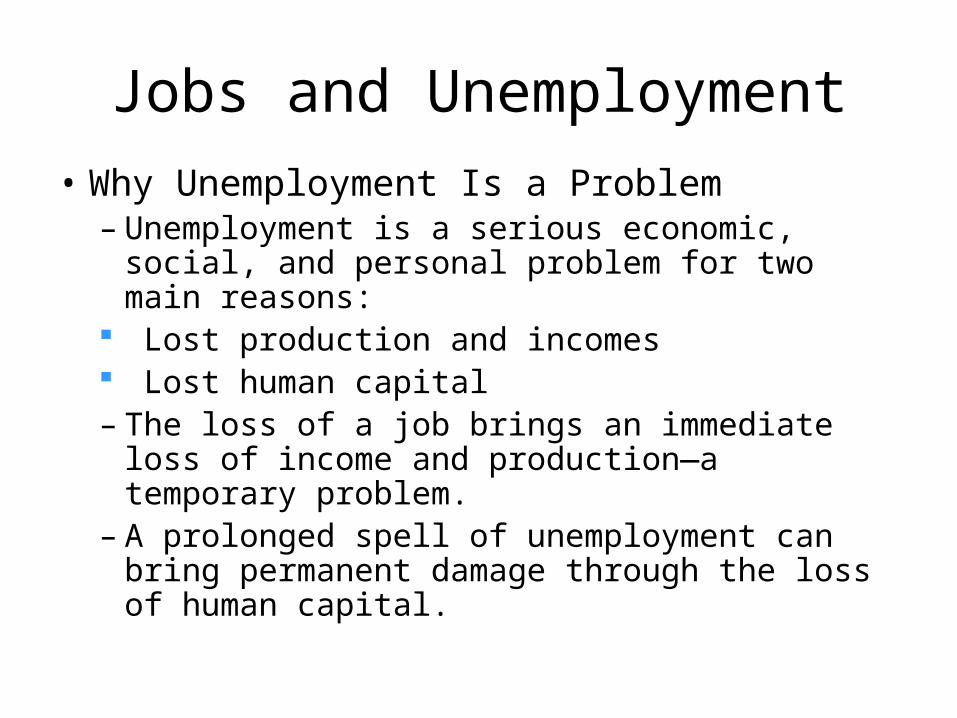
Jobs and Unemployment• Why Unemployment Is a Problem– Unemployment is a serious economic, social, and
personal problem for two main reasons: Lost production and incomes Lost human capital– The loss of a job brings an immediate loss of
income and production—a temporary problem.– A prolonged spell of unemployment can bring
permanent damage through the loss of human capital.

Inflation and the Dollar
– We measure the level of prices—the price level— as the average of the prices that people pay for all the goods and services that they buy.
– The Consumer Price Index—the CPI—is a common measure of the price level.
– We measure the inflation rate as the percentage change in the price level.
– Inflation arises when the price level is rising persistently.
– If the price level is falling, inflation is negative and we have deflation.
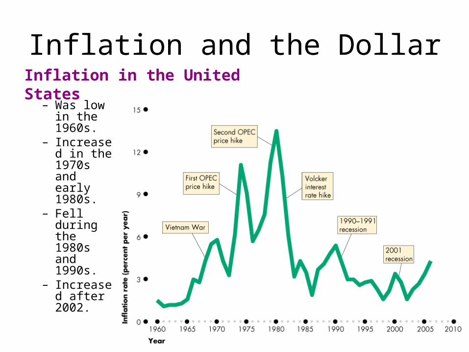
Inflation and the Dollar
– Was low in the 1960s.
– Increased in the 1970s and early 1980s.
– Fell during the 1980s and 1990s.
– Increased after 2002.
Inflation in the United States

Inflation and the Dollar
• Inflation Around the World– Figure (a) shows the
inflation rate in the United States compared with that in other industrial countries.
– U.S. inflation is similar to that in other industrial countries.

Inflation and the Dollar
– Figure (b) shows the inflation rate in industrial countries has been much lower than that in developing countries.
Inflation and the Dollar
• Hyperinflation– The most serious type of inflation is hyperinflation—
an inflation rate that exceeds 50 percent a month.– Why Inflation is a Problem – Inflation is a problem for many reasons, but the main
one is that once it takes hold, it is unpredictable. – Unpredictable inflation is a problem because it Redistributes income and wealth Diverts resources from production

Inflation and the Dollar
– Unpredictable changes in the inflation rate redistribute income in arbitrary ways between employers and workers and between borrowers and lenders.
– A high inflation rate is a problem because it diverts resources from productive activities to inflation forecasting.
– From a social perspective, this waste of resources is a cost of inflation.
– Eradicating inflation is costly because it brings a period of greater than average unemployment.

Inflation and the Dollar
• The Value of the Dollar– The value of the U.S. dollar in terms of other
currencies is called the exchange rate—a measure of how much your dollar will buy in other parts of the world.
– An example is the number of pesos that 1 U.S. dollar will buy.

Surpluses, Deficits, and Debts
– Figure shows the U.S. dollar exchange rate.
– When value of the dollar decreases, the U.S. dollar depreciates against other currencies.
– When value of the dollar increases, the U.S. dollar appreciates against other currencies.

Inflation and the Dollar
• Why the Exchange Rate Matters– When the U.S. dollar appreciates, U.S. consumers
pay less for imported goods.– But the higher dollar makes it harder for U.S.
producers to complete in foreign markets. A higher dollar hurts U.S producers.
– When the U.S. dollar depreciates, U.S. consumers pay more for imported goods. So a lower dollar hurts consumers.
– But the lower dollar makers it easier for U.S. producers to complete in foreign markets.
Surpluses, Deficits, and Debts
• Government Budget Balance– If a government collects more in taxes than it spends,
it has a government budget surplus. – If a government spends more than it collects in taxes,
it has a government budget deficit.
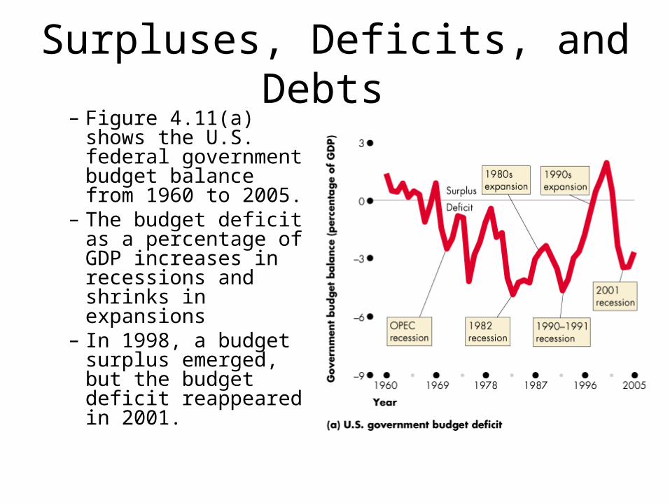
Surpluses, Deficits, and Debts – Figure 4.11(a) shows
the U.S. federal government budget balance from 1960 to 2005.
– The budget deficit as a percentage of GDP increases in recessions and shrinks in expansions
– In 1998, a budget surplus emerged, but the budget deficit reappeared in 2001.

Surpluses, Deficits, and Debts
• International Surplus and Deficit– If a nation imports more than it exports, it has an
international deficit.– If a nation exports more than it imports, it has an
international surplus.– The balance on the current account equals U.S.
exports minus U.S. imports but also takes into account interest payments paid to and received from the rest of the world.

Surpluses, Deficits, and Debts – Figure 4.11(b) shows
the U.S. current account balance from 1960 to 2005.
– During the 1980s expansion, a large deficit appeared but it almost disappeared during the 1990–1991 recession.
– The current account deficit in 2005 was 6.3 percent of GDP.
Surpluses, Deficits, and Debts
• Deficits Bring Debts– A debt is the amount that is owed.– When a government or a nation has a deficit, its
debt grows.– A government’s or a nation’s debt equals the sum
of all past deficits minus past surpluses. – A government’s debt is called national debt.

Surpluses, Deficits, and Debts
– Figure (a) shows the U.S. government debt from 1945 to 2005.
– Budget surpluses and rapid economic growth shrink the debt.
– Budget deficits and slower economic growth swelled the debt.
Surpluses, Deficits, and Debts
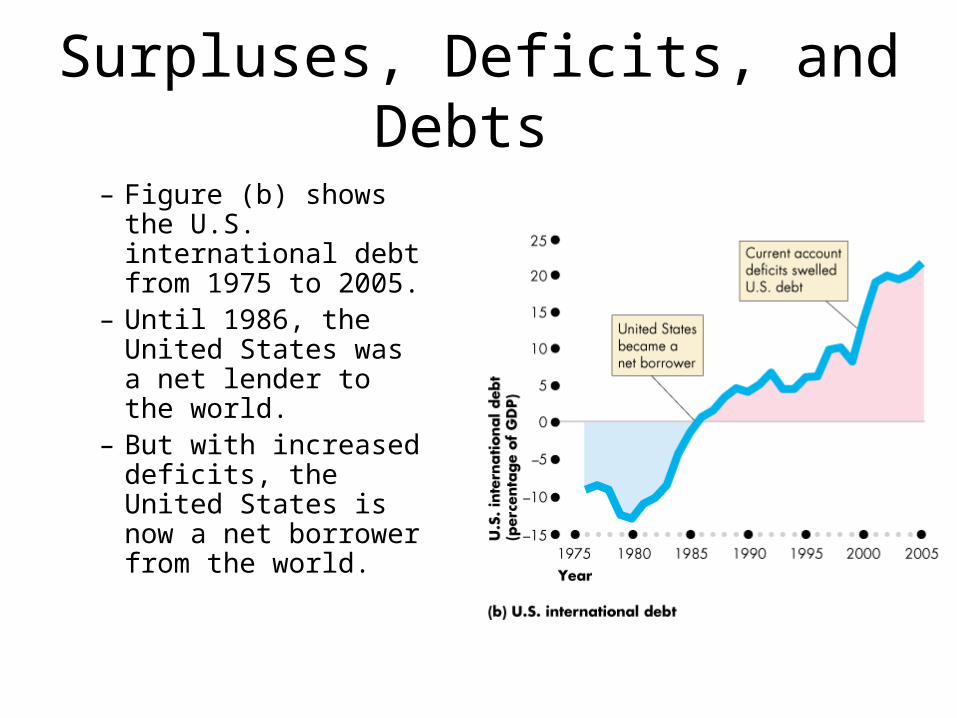
– Figure (b) shows the U.S. international debt from 1975 to 2005.
– Until 1986, the United States was a net lender to the world.
– But with increased deficits, the United States is now a net borrower from the world.

Assets Liabilities and Net Worth
Creating a Bank
• Creating a Bank
• Vault Cash
Creating a BankBalance Sheet 1: Wahoo Bank
Cash $250,000 Stock Shares $250,000

Assets Liabilities and Net Worth
Creating a Bank• Acquiring Property and
Equipment
Acquiring Property and EquipmentBalance Sheet 2: Wahoo Bank
Cash $10,000 Stock Shares $250,000Property $240,000
Assets Liabilities and Net Worth
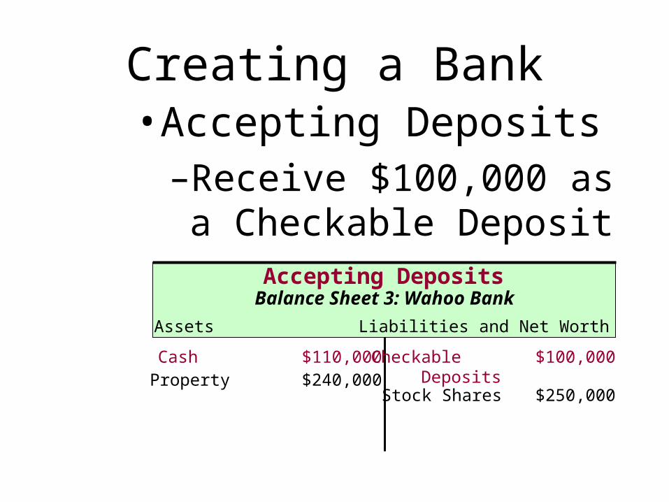
Creating a Bank• Accepting Deposits–Receive $100,000 as a
Checkable DepositAccepting Deposits
Balance Sheet 3: Wahoo Bank
Cash $110,000 Checkable Deposits
$100,000Property $240,000
Stock Shares $250,000

Creating a Bank• Depositing Reserves in a
Federal Reserve Bank–Required Reserves–Reserve Ratio
:
ReserveRatio =
Commercial Bank’sRequired Reserves
Commercial Bank’sCheckable-Deposit Liabilities

Assets Liabilities and Net Worth
Creating a Bank
Depositing Reserves at the FedBalance Sheet 4: Wahoo Bank
Cash $0 Checkable Deposits $100,000
Property $240,000 Stock Shares $250,000
Type of DepositCurrent
RequirementStatutory
Limits
Checkable Deposits:$0-$7.8 Million$6-$48.3 MillionOver $48.3 Million
Noncheckable NonpersonalSavings and Time Deposits
0% 310
3% 38-14
0 0-9
Reserves $110,000

Creating a Bank
Excess Reserves
ExcessReserves = -Actual
ReservesRequiredReserves
Assets Liabilities and Net Worth
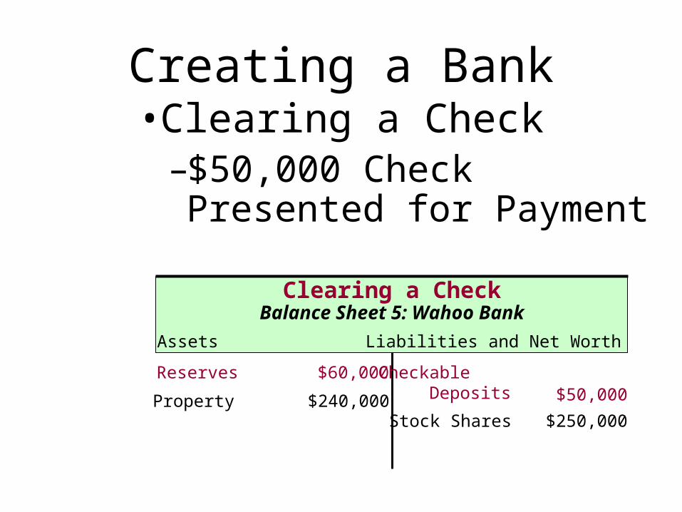
Creating a Bank
Clearing a CheckBalance Sheet 5: Wahoo Bank
Checkable Deposits $50,000Property $240,000Stock Shares $250,000
Reserves $60,000
• Clearing a Check–$50,000 Check Presented
for Payment

Assets Liabilities and Net Worth
Money Creating Transactions:
When a Loan is NegotiatedBalance Sheet 6a: Wahoo Bank
Checkable Deposits $100,000
Property $240,000 Stock Shares $250,000
Reserves $60,000
• Granting a Loan–$50,000 Loan Deposited to
Checking Account
Loans $50,000
Assets Liabilities and Net Worth
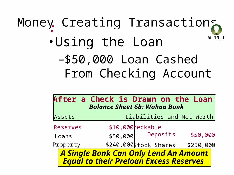
Money Creating Transactions:
After a Check is Drawn on the Loan Balance Sheet 6b: Wahoo Bank
Checkable Deposits $50,000
Property $240,000 Stock Shares $250,000
Reserves $10,000
• Using the Loan–$50,000 Loan Cashed From
Checking Account
Loans $50,000
A Single Bank Can Only Lend An AmountEqual to their Preloan Excess Reserves
W 13.1

Assets Liabilities and Net Worth
Money Creating Transactions
Buying Government SecuritiesBalance Sheet 7: Wahoo Bank
Checkable Deposits $100,000
Property $240,000 Stock Shares $250,000
Reserves $60,000
• Buying Government Securities From Dealer–Deposits Payment Into Checking
Account
Securities $50,000

The Banking System
Bank ABank BBank CBank DBank EBank FBank GBank HBank IBank JBank KBank LBank MBank NOther Banks
Bank
(1)AcquiredReserves
and Deposits
(2)RequiredReserves(Reserve
Ratio = .2)
(3)Excess
Reserves(1)-(2)
(4)Amount Bank CanLend; New Money
Created = (3)
$100.0080.0064.0051.2040.9632.7726.2120.9716.7813.4210.74
8.596.875.50
21.99
$20.0016.0012.8010.24
8.196.555.244.203.362.682.151.721.371.104.40
$80.0064.0051.2040.9632.7726.2120.9716.7813.4210.74
8.596.875.504.40
17.59
$80.0064.0051.2040.9632.7726.2120.9716.7813.4210.74
8.596.875.504.40
17.59$400.00
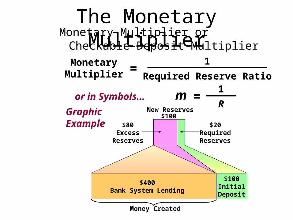
The Monetary MultiplierMonetary Multiplier or Checkable-Deposit MultiplierMonetaryMultiplier =
1
Required Reserve Ratio
or in Symbols… m =1
RNew Reserves
$100$20
RequiredReserves
$80Excess
Reserves
$100Initial
Deposit
$400Bank System Lending
Money Created
GraphicExample

Interest Rates• Equilibrium Interest Rate• Interest Rates and Bond Prices–Bond Prices Fall When
Interest Rates Rise–Bond Prices Rise When
Interest Rates Fall–Inverse Relationship Between
Interest Rates and Bond Prices
W 14.2
G 14.1
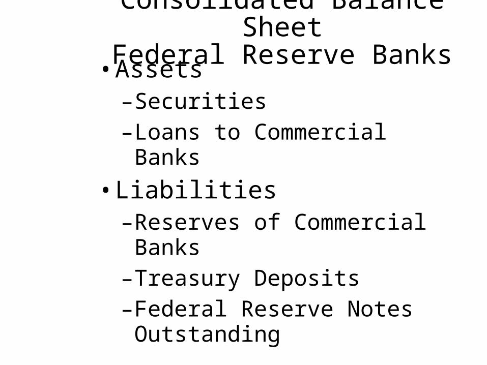
Consolidated Balance SheetFederal Reserve Banks
• Assets–Securities–Loans to Commercial Banks
• Liabilities–Reserves of Commercial Banks–Treasury Deposits–Federal Reserve Notes
Outstanding

Consolidated Balance SheetFederal Reserve Banks
SecuritiesLoans to Commercial BanksAll Other Assets
Total
Reserves of Commercial BanksTreasury DepositsFederal Reserve Notes (Outstanding)All Other Liabilities and Net WorthTotal
Consolidated Balance Sheet of the 12 Federal Reserve BanksMarch 29, 2006 (in Millions)
Assets Liabilities and Net Worth
Source: Federal Reserve Statistical Release, H.4.1, May 7, 2003
$758,551
19,25059,967
$837,768
$ 14,9234,463
754,56763,615
$837,768

Tools of Monetary Policy• Open Market Operations–Buying Securities• From Commercial Banks• From the Public
–Selling Securities• To Commercial Banks• To the Public
• When the Fed Sells Securities, Commercial Bank Reserves are Reduced
O 14.2
W 14.3
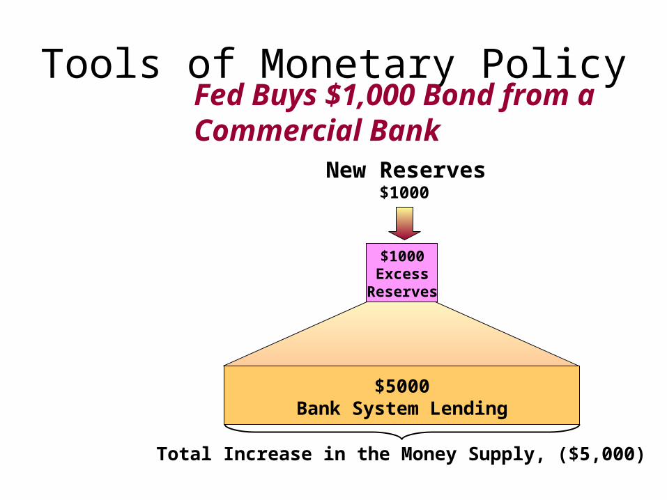
Tools of Monetary Policy
New Reserves$1000
$5000Bank System Lending
Total Increase in the Money Supply, ($5,000)
Fed Buys $1,000 Bond from a Commercial Bank
$1000Excess
Reserves

Tools of Monetary Policy
Check is DepositedNew Reserves
$1000
Total Increase in the Money Supply, ($5000)
Fed Buys $1,000 Bond from the Public
$200RequiredReserves
$800Excess
Reserves
$1000Initial
CheckableDeposit
$4000Bank System Lending

Tools of Monetary Policy• The Reserve Ratio–Raising the Reserve Ratio–Lowering the Reserve Ratio
• The Discount Rate–Borrowing from the Fed by
Banks Increases Reserves and Enhances Lending Ability
• Relative Importance of Each
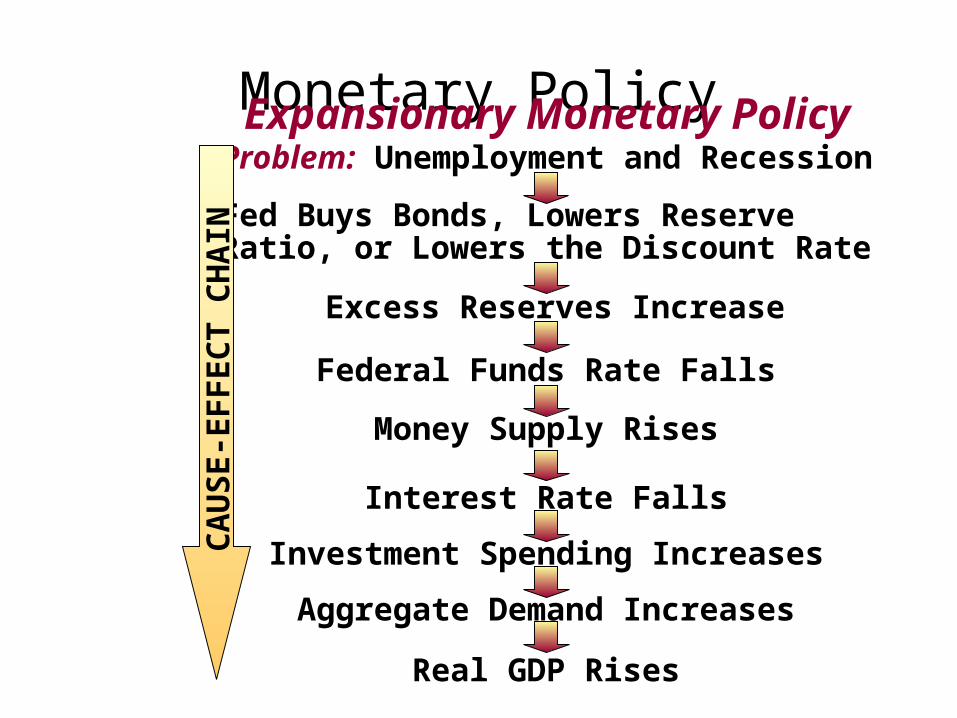
Monetary PolicyExpansionary Monetary PolicyProblem: Unemployment and Recession
Fed Buys Bonds, Lowers ReserveRatio, or Lowers the Discount Rate
Excess Reserves Increase
Federal Funds Rate Falls
Money Supply Rises
Interest Rate Falls
Investment Spending Increases
Aggregate Demand Increases
Real GDP Rises
CAU
SE-E
FFEC
T CH
AIN

Monetary PolicyRestrictive Monetary PolicyProblem: Inflation
Fed Sells Bonds, Increases ReserveRatio, or Increases the Discount Rate
Excess Reserves Decrease
Federal Funds Rate Rises
Money Supply Falls
Interest Rate Rises
Investment Spending Decreases
Aggregate Demand Decreases
Inflation Declines
CAU
SE-E
FFEC
T CH
AIN