Application of Mixture Theory

to solid tumors andnormal pressure hydrocephalus

by

Andrijana Burazin

A thesis

presented to the University of Waterloo

in fulfillment of the

thesis requirement for the degree of

Doctor of Philosophy

in

Applied Mathematics

Waterloo, Ontario, Canada, 2013

c© Andrijana Burazin 2013

I hereby declare that I am the sole author of this thesis. This is a true copy of the thesis,

including any required final revisions, as accepted by my examiners.

I understand that my thesis may be made electronically available to the public.

ii

Abstract

In this Thesis, the theory of poroelasticity, namely the Mixture Theory version – a ho-

mogenized, macroscopic scale approach used to describe fluid flow through a porous medium

– is employed in three separate cases pertaining to a biological phenomenon.

The first investigation explores the behavior of interstitial fluid pressure (IFP) in solid

tumors. Thus, in Chapter 2, a Mixture Theory based approach is developed to describe the

evolution of the IFP from that in a healthy interstitium to the elevated levels in cancerous

tumors. Attention is focused on angiogenesis, a tightly regulated process in healthy tissue

that provides all necessary nutrients through the creation of new blood vessels. Once this

process becomes unruly within a tumor, angiogenesis gives rise to an abnormal vasculature

by forming convoluted and leaky blood vessels. Thus, the primary focus of the model is on

the capillary filtration coefficient and vascular density as they increase in time, which in turn

elevates the tumor IFP. Later, the Mixture Theory model is extended to simulate the effects

of vascular normalization, where the cancer therapy not only prunes blood vessels, but reverts

the chaotic vasculature to a somewhat normal state, thereby temporarily lowering the tumor

IFP.

In Chapter 3, the validity of an assumption that was made in order to facilitate the math-

ematical calculations is investigated. In addition to all of the Mixture Theory assumptions, it

is assumed that the pore pressure p is proportional to the tissue dilatation e. This assumption

is examined to determine how appropriate and accurate it is, by using a heat type equation

without the presence of sources and sinks under the assumption of a spherical geometry. The

results obtained under the proportionality of p and e, are compared with the results obtained

without this assumption. A substantial difference is found, which suggests that great care

must be exercised in assuming the proportionality of p and e.

The last application is reported in Chapter 4 and it investigates the pathogenesis of

normal pressure hydrocephalus. In a normal brain, cerebrospinal fluid (CSF) is created by

the choroid plexus, circulates around the brain and the spinal cord without any impediment,

and then is absorbed at various sites. However, normal pressure hydrocephalus occurs when

there is an imbalance between the production and absorption of CSF in the brain that causes

the impaired clearance of CSF and the enlargement of ventricles; however, the ventricular

iii

pressure in this case is frequently measured to be normal. Thus, a mathematical model

using Mixture Theory is formulated to analyze a possible explanation of this brain condition.

Levine (1999) proposed the hypothesis that CSF seeps from the ventricular space into the

brain parenchyma and is efficiently absorbed in the bloodstream. To test this hypothesis,

Levine used the consolidation theory version of poroelasticity theory, with the addition of

Starling’s law to account for the absorption of CSF in the brain parenchyma at steady state.

However, the Mixture Theory model does not agree with the results obtained by Levine

(1999) which leads one to conclude that the pathogenesis of normal pressure hydrocephalus

remains unknown.

To conclude the Thesis, all three applications of Mixture Theory are discussed and the

importance and contribution of this work is highlighted. In addition, possible future directions

are indicated based on the findings of this Thesis.

iv

Acknowledgements

Dr. Tenti has been a great inspiration throughout my PhD journey at UW, and I will

forever be indebt and grateful to him for his mentoring. He has enlightened me with knowledge

and has encouraged me throughout the good times and the bad times to become more self-

confident. None of my efforts, especially this thesis, would have been possible without him.

Dr. Sivaloganathan with his good spirits and sense of humor always had a calm demeanor

in any situation. I will forever admire his dedication to the Biomedical research group - in

the way he bridges multidisciplinary research to tackle biomedical problems. And thus, this

thesis would not have been the same without his editing and piecing of ideas together.

I would like to thank all the past and present members of the Biomedical research group.

You have helped me grow - academically and non-academically alike. I wish you all the best

in your future endeavors.

Helen Warren, you have been a wonderful help and very motherly, especially when I had

my conundrums and odd ends to figure out. Stephanie Evers, you have been awesome, and I

truly appreciated our conversations.

To my loving family, this definitely would not have been easy without you all! Thanks

Chris for your support and being there, and of course, for your alma mater card.

v

For dd.

vi

Contents

List of Tables x

List of Figures xi

1 Introduction 1

2 Formulation of the tumor interstitial fluid pressure problem 8

2.1 Introduction . . . . . . . . . . . . . . . . . . . . . . . . . . . . . . . . . . . . . . . . . . . . . . . . . . . . . . . . . . . . . . . . . . . 8

2.2 Formulation of the mathematical model . . . . . . . . . . . . . . . . . . . . . . . . . . . . . . . . . . . . . . . . .9

2.3 Solution . . . . . . . . . . . . . . . . . . . . . . . . . . . . . . . . . . . . . . . . . . . . . . . . . . . . . . . . . . . . . . . . . . . . . . .15

2.3.1 Steady state . . . . . . . . . . . . . . . . . . . . . . . . . . . . . . . . . . . . . . . . . . . . . . . . . . . . . . . . . . . . .15

2.3.2 Transient state . . . . . . . . . . . . . . . . . . . . . . . . . . . . . . . . . . . . . . . . . . . . . . . . . . . . . . . . . . 16

2.4 Parameters . . . . . . . . . . . . . . . . . . . . . . . . . . . . . . . . . . . . . . . . . . . . . . . . . . . . . . . . . . . . . . . . . . . .18

2.5 Results. . . . . . . . . . . . . . . . . . . . . . . . . . . . . . . . . . . . . . . . . . . . . . . . . . . . . . . . . . . . . . . . . . . . . . . .22

2.5.1 Steady state . . . . . . . . . . . . . . . . . . . . . . . . . . . . . . . . . . . . . . . . . . . . . . . . . . . . . . . . . . . . .23

2.5.2 Transient state . . . . . . . . . . . . . . . . . . . . . . . . . . . . . . . . . . . . . . . . . . . . . . . . . . . . . . . . . . 24

2.6 Application to anti-angiogenesis therapy . . . . . . . . . . . . . . . . . . . . . . . . . . . . . . . . . . . . . . . 32

3 Testing the approximation (2μ + λ)e(r, t) = p(r, t) in a hollow 43

spherically symmetric domain

vii

3.1 Introduction . . . . . . . . . . . . . . . . . . . . . . . . . . . . . . . . . . . . . . . . . . . . . . . . . . . . . . . . . . . . . . . . . . 43

3.1.1 Some details of De Leeuw (1965) argument . . . . . . . . . . . . . . . . . . . . . . . . . . . . . . 45

3.1.2 Case of spherically symmetric sand drain . . . . . . . . . . . . . . . . . . . . . . . . . . . . . . . . 47

3.2 Step 1: Approximated case . . . . . . . . . . . . . . . . . . . . . . . . . . . . . . . . . . . . . . . . . . . . . . . . . . . . 48

3.3 Steps 2 and 3: Test case . . . . . . . . . . . . . . . . . . . . . . . . . . . . . . . . . . . . . . . . . . . . . . . . . . . . . . .51

3.4 Step 4: Comparison . . . . . . . . . . . . . . . . . . . . . . . . . . . . . . . . . . . . . . . . . . . . . . . . . . . . . . . . . . . 58

3.4.1 Parameters . . . . . . . . . . . . . . . . . . . . . . . . . . . . . . . . . . . . . . . . . . . . . . . . . . . . . . . . . . . . . .59

3.4.2 Results . . . . . . . . . . . . . . . . . . . . . . . . . . . . . . . . . . . . . . . . . . . . . . . . . . . . . . . . . . . . . . . . . .59

4 Examining the behavior of normal pressure hydrocephalus 66

4.1 Review of the work done by Levine (1999) . . . . . . . . . . . . . . . . . . . . . . . . . . . . . . . . . . . . . 66

4.1.1 Radial steady state pressure distribution of parenchymal tissue . . . . . . . . . . .67

4.1.2 Radial steady state displacement distribution of parenchymal tissue . . . . . . 69

4.2 Radial steady state pressure and displacement distribution in . . . . . . . . . . . . . . . . . . 72

normal pressure hydrocephalus according to mixture theory

4.2.1 Radial steady state pressure . . . . . . . . . . . . . . . . . . . . . . . . . . . . . . . . . . . . . . . . . . . . . 72

4.2.2 Radial steady state displacement . . . . . . . . . . . . . . . . . . . . . . . . . . . . . . . . . . . . . . . . 75

4.3 Results. . . . . . . . . . . . . . . . . . . . . . . . . . . . . . . . . . . . . . . . . . . . . . . . . . . . . . . . . . . . . . . . . . . . . . . .78

4.3.1 Parameters . . . . . . . . . . . . . . . . . . . . . . . . . . . . . . . . . . . . . . . . . . . . . . . . . . . . . . . . . . . . . .78

4.3.2 Radial steady state pressure distribution . . . . . . . . . . . . . . . . . . . . . . . . . . . . . . . . .80

4.3.3 Radial steady state displacement distribution . . . . . . . . . . . . . . . . . . . . . . . . . . . . 83

5 Discussion and conclusion 86

viii

Appendix A: Formulation of mixture theory 91

Appendix B: Relation between tissue dilatation and 96

interstitial fluid pressure

Appendix C: Calculations of analytic solution for the approximated case 98

in Chapter 3

Appendix D: Calculations of constants to the general solution 100

in Chapter 3

References 105

ix

List of Tables

Table 2.1: Model parameter values . . . . . . . . . . . . . . . . . . . . . . . . . . . . . . . . . . . . . . . . . . . . . . . . . . . . . .19

Table 2.2: Parameter T values for various elastic materials . . . . . . . . . . . . . . . . . . . . . . . . . . . . . . 20

Table 2.3: Parameter values for frequency D and time scale t∗ . . . . . . . . . . . . . . . . . . . . . . . . . . .21

Table 2.4: Parameter values for frequency F and time scale t∗∗ . . . . . . . . . . . . . . . . . . . . . . . . . . 22

Table 2.5: Values for vascular density SV and parameter E . . . . . . . . . . . . . . . . . . . . . . . . . . . . . . .29

Table 2.6: Anti-angiogenesis therapy timeline . . . . . . . . . . . . . . . . . . . . . . . . . . . . . . . . . . . . . . . . . . . 34

Table 2.7: Values for vascular density SV in anti-angiogenesis therapy timeline. . . . . . . . . . . .39

Table 3.1: Hollow sphere radii values. . . . . . . . . . . . . . . . . . . . . . . . . . . . . . . . . . . . . . . . . . . . . . . . . . . .59

Table 4.1: Parameter values for A2 and k . . . . . . . . . . . . . . . . . . . . . . . . . . . . . . . . . . . . . . . . . . . . . . . 79

Table 4.2: Levine (1999) Lame coefficient values with fixed ν = 0.35 . . . . . . . . . . . . . . . . . . . . . 80

Table 4.3: Ventricular displacement ur(ri) according to the mixture theory model . . . . . . . 84

Table 4.4: Ventricular displacement ur(ri) according to the elastic . . . . . . . . . . . . . . . . . . . . . . .84

parameters suggested by Levine (1999) with ri = 4 cm

x

List of Figures

Figure 1.1: Geometry of the brain parenchyma . . . . . . . . . . . . . . . . . . . . . . . . . . . . . . . . . . . . . . . . . . . 6

Figure 2.1: IFP steady state profile . . . . . . . . . . . . . . . . . . . . . . . . . . . . . . . . . . . . . . . . . . . . . . . . . . . . . 23

Figure 2.2: Behavior of α(t) modeled by Lp(t) with D1 = 130 second−1 . . . . . . . . . . . . . . . . . . . 25

Figure 2.3: Behavior of α(t) modeled by Lp(t) with D2 = 1 day−1 . . . . . . . . . . . . . . . . . . . . . . . 26

Figure 2.4: Behavior of α(t) modeled by Lp(t) with D3 = 13 day−1 . . . . . . . . . . . . . . . . . . . . . . . 26

Figure 2.5: Transient IFP profile modeled by Lp(t) with D1 = 130 second−1 . . . . . . . . . . . . . . 27

Figure 2.6: Transient IFP profile modeled by Lp(t) with D2 = 1 day−1 . . . . . . . . . . . . . . . . . . 28

Figure 2.7: Transient IFP profile modeled by Lp(t) with D3 = 13 day−1 . . . . . . . . . . . . . . . . . . 28

Figure 2.8: Behavior of α(t) modeled by SV (t) with F2 = 1

7 day−1 . . . . . . . . . . . . . . . . . . . . . . . . 30

Figure 2.9: Behavior of α(t) modeled by SV (t) with F4 = 1

16 day−1 . . . . . . . . . . . . . . . . . . . . . . . 30

Figure 2.10: Evolution of IFP modeled by SV (t) with F2 = 1

7 day−1 . . . . . . . . . . . . . . . . . . . . . . 31

Figure 2.11: Evolution of IFP modeled by SV (t) with F4 = 1

16 day−1 . . . . . . . . . . . . . . . . . . . . . 32

Figure 2.12: Evolution of IFP modeled by Lp(t) with M = 13 day−1 . . . . . . . . . . . . . . . . . . . . . .36

Figure 2.13: Evolution of IFP modeled by Lp(t) with SV = 20, 30 and 40 cm−1 . . . . . . . . . . .37

xi

Figure 2.14: Evolution of IFP modeled by Lp(t) with M = 1, 13 and 1

5 day−1 . . . . . . . . . . . . 37

Figure 2.15: Evolution of IFP modeled by SV (t) with S = 1

5 day−1 . . . . . . . . . . . . . . . . . . . . . . . 40

Figure 2.16: Evolution of IFP modeled by SV (t) with S

V

N= 20, 30 and 40 cm−1 . . . . . . . . . .41

Figure 2.17: Evolution of IFP modeled by SV (t) with S = 1

3 , 15 and 1

7 day−1 . . . . . . . . . . . . . .41

Figure 3.1: Hollow cylindrical domain . . . . . . . . . . . . . . . . . . . . . . . . . . . . . . . . . . . . . . . . . . . . . . . . . . .46

Figure 3.2: Hollow spherical domain . . . . . . . . . . . . . . . . . . . . . . . . . . . . . . . . . . . . . . . . . . . . . . . . . . . . 49

Figure 3.3: Pressure profile for soft saturated clay with . . . . . . . . . . . . . . . . . . . . . . . . . . . . . . . . . .60

the inner and outer radii of 0.2 cm and 0.5 cm

Figure 3.4: Pressure profile for soft saturated clay with . . . . . . . . . . . . . . . . . . . . . . . . . . . . . . . . . .61

the inner and outer radii of 0.5 cm and 1 cm

Figure 3.5: Pressure profile for soft saturated clay with . . . . . . . . . . . . . . . . . . . . . . . . . . . . . . . . . .61

the inner and outer radii of 5 cm and 10 cm

Figure 3.6: Pressure profile for very soft saturated clay with . . . . . . . . . . . . . . . . . . . . . . . . . . . . .62

the inner and outer radii of 0.2 cm and 0.5 cm

Figure 3.7: Pressure profile for very soft saturated clay with . . . . . . . . . . . . . . . . . . . . . . . . . . . . .63

the inner and outer radii of 0.5 cm and 1 cm

Figure 3.8: Pressure profile for very soft saturated clay with . . . . . . . . . . . . . . . . . . . . . . . . . . . . .63

the inner and outer radii of 5 cm and 10 cm

Figure 3.9: Transient state profile for medium saturated clay with . . . . . . . . . . . . . . . . . . . . . . . 64

the inner and outer radii of 0.2 cm and 0.5 cm

xii

Figure 3.10: Transient state profile for medium saturated clay with . . . . . . . . . . . . . . . . . . . . . .64

the inner and outer radii of 0.5 cm and 1 cm

Figure 3.11: Transient state profile for medium saturated clay with . . . . . . . . . . . . . . . . . . . . . .65

the inner and outer radii of 5 cm and 10 cm

Figure 4.1: Steady state pressure profile with A21 = 7.2 cm−2 . . . . . . . . . . . . . . . . . . . . . . . . . . . . 81

Figure 4.2: Steady state pressure profile with A22 = 21.6 cm−2 . . . . . . . . . . . . . . . . . . . . . . . . . . .82

Figure 4.3: Steady state pressure profile with A23 = 36 cm−2 . . . . . . . . . . . . . . . . . . . . . . . . . . . . .82

Figure 4.4: Steady state pressure profile with A24 = 10 cm−2 . . . . . . . . . . . . . . . . . . . . . . . . . . . . .83

xiii

Chapter 1

Introduction

The aim of this Thesis is to report the results of three separate investigations with a

common theme – the application of the theory of poroelasticity via the Mixture Theory

approach, to biological tissue.

The first application – reported in Chapter 2 – is of interest to oncological research, as it

investigates the behavior of interstitial fluid pressure (IFP) in solid tumors. For quite a long

time, IFP has been known to be higher than the hydrostatic pressure of healthy interstitium.

Young et al. (1950) claimed that the IFP may be an essential factor in the dissemination

of malignant tumors. Their experimental results showed that the IFP of tumors is higher

than that of normal tissue. This phenomenon has been confirmed by other studies of solid

tumors (Guillino et al., 1964), also covering many types of cancers such as breast carcinoma

(Less et al., 1992; Nathanson and Nelson, 1994), metastatic melanoma (Curti et al., 1993;

Boucher et al., 1991), and neck carcinoma (Gutman et al., 1992). In spite of the advances,

the mechanism responsible for the increased IFP remained obscure.

A breakthrough in understanding the elevated IFP phenomenon occurred when Jain

(1987a, 1987b) identified a key problem in cancer treatment. He claimed that due to the

increased IFP, therapeutic agents are not distributed adequately and uniformly within a

tumor. Once administered, the drug agents were found to be located around the blood vessels

and in some instances in abundance within the outer edge of the tumor. Consequently, no

desired therapeutic effects occurred in the center of the tumor. Baxter and Jain (1989)

suggested that the elevated IFP, acting as an adverse pressure gradient, limits the transport

in tumors. This, in turn, causes a reduction of the driving force for transvascular exchange

of both fluid and macromolecules.

To describe the IFP behavior in a solid tumor, Baxter and Jain (1989) developed a

mathematical model. Macroscopically, the solid tumor is modeled as spherical in shape,

1

homogeneous, tissue-isolated, and without a necrotic core. The tumor interstitium is viewed

as a rigid porous medium where the fluid flow is regulated by Darcy’s law. Assuming that the

lymphatic drainage and oncotic pressure are negligible (Jain et al., 2007), the transcapillary

exchange of fluid is governed by Starling’s law. Using the two laws that govern the transport

process in a solid tumor, an explicit formula for the steady state IFP is derived. When

expressed in dimensionless form, this formula depends only on the dimensionless tumor radius

and a dimensionless parameter

α = R

√Lp

K

S

V, (1.1)

where R is the tumor radius (cm), SV is the vascular surface area per unit volume (cm−1), Lp

is the capillary permeability of the microvascular wall (cm second−1 mmHg−1), and K is the

hydraulic conductivity of the interstitium (cm2 second−1 mmHg−1); all of these parameters

are assumed constant.

The model by Baxter and Jain (1989) was extended several years later to include the

time-dependent behavior of the IFP in solid tumors (Netti et al., 1995, 1997), by using

the Mixture Theory approach (Kenyon, 1976a,b). In these attempts the transient IFP was

studied in the following manner: by starting from the elevated steady state IFP value and

artificially disturbing this equilibrium by increasing the vascular pressure and then, after the

IFP had reached a stable value, a decrease in the vascular pressure caused IFP to return

to its initial value. The results of this simulation showed that the IFP near the center of

the tumor followed very closely the changes in the microvascular pressure, with a delay of

only a few seconds. Intuitively, this behavior is the result of the form of the volumetric flow

rate out of the vasculature per unit volume. In the simplest case of negligible lymphatic and

oncotic gradients, this flux is given by JvV = LpS

V (pv − p), where pv is the blood pressure and

p is the IFP, both having the units in mmHg. Since Lp and SV are taken to be constant,

an increase of pv will increase the flux. Also, since the tumor hydraulic conductivity K is

kept constant, the increasing flux will elevate the IFP in order to maintain the equilibrium.

Furthermore, the tumor value of the capillary filtration coefficient LpSV is very high due to

the excess leakiness of the capillary walls; hence, extravasation will be very rapid once the

blood pressure is raised.

The conclusions drawn from these mathematical models offered useful insights into the

causes of the elevated tumor IFP, but by no means provided a definitive explanation of the

2

mechanisms responsible for the phenomenon. In particular, the constancy (as well as the

actual value) of the tumor hydraulic conductivity K has been questioned. For instance,

Khosvarani et al. (2004) found experimentally that the response time of the tumor IFP to a

perturbation of the steady state can be substantially different from one tumor to the next,

and is strongly influenced by the value of K. A few years later Milosevic et al. (2008) re-

analyzed the data using a more refined mathematical model, and estimated the values of K

for different tumors.

In Chapter 2, a macroscopic mathematical model is developed to describe the time evo-

lution of a tumor IFP. The attention is placed on the mechanisms which are responsible for

the rise of the IFP from its value in healthy interstitium to the measured value in a cancerous

state.

As an organ grows, all necessary nutrients are supplied through the creation of new blood

vessels (angiogenesis). In healthy tissue angiogenesis is a tightly regulated process, in which

the onset and offset mechanisms are controlled by a large number of molecular and mechanical

factors (Carmeliet and Jain, 2011; Jain, 2003). The parameter α defined in (1.1) is constant.

In contrast, as demonstrated by Gullino (1976), the cells in cancerous tissue acquire the

ability to stimulate angiogenesis. Proceeding in an unregulated fashion, angiogenesis gives

rise to an abnormal vasculature with blood vessels that are saccular, convoluted, leaky, and

have defects in pericyte coverage and function due to the over-expression of the vascular

endothelial growth factor (VEGF) signalling protein (Heldin et al., 2004). Thus, as the

tumor evolves, the capillary filtration coefficient and the vascular density increase and the

parameter α becomes dependent on time.

The Mixture Theory model is further employed to simulate the effect of ‘vascular normal-

ization’of the IFP profile. The hypothesis of vascular normalization, proposed by Jain (2001,

2005), postulates that anti-angiogenesis therapy does not just prune vessels, but reverts the

abnormal vascular structure and function toward a more normal state, thereby lowering the

tumor IFP for a short period of time.

The second application – detailed in Chapter 3 – is more mathematical in nature, and

bears relevance to the work in Chapter 2. In the model in Chapter 2, on top of the require-

ments needed for the Mixture Theory, it is assumed that the pore pressure p and the tissue

dilatation e are proportional. As a result, the fundamental partial differential equations of

3

poroelasticity theory reduce to a standard heat-type equation for the pore pressure in the

case of no sources, or to the simplest case of a reaction-diffusion equation when sources are

present. This assumption is used in previous models which investigate the behavior of IFP in

solid tumors (Netti et al., 1995, 1997), and is clearly of interest to determine how appropriate

and accurate it is.

In contrast to the application of poroelasticity theory to solid tumors, this proportional-

ity assumption problem is well known (Bear, 1988), and has been studied in the context of

a groundwater flow (Verruijt, 1969). The approximation has been found to be either good

or bad, depending on the geometry of the system and the type of boundary conditions pre-

scribed. However, no general test of the approximation has been made. An exception among

these studies is De Leeuw (1965), where the necessary and sufficient conditions for the exact

proportionality between p and e were identified in the special case of a vertical cylindrical

sand drain satisfying the conditions of plane strain and axial symmetry.

Since the paper by De Leeuw (1965) is not readily accessible, Chapter 3 starts with a

detailed review of his work. For simplicity, the mathematical model developed there using

Mixture Theory assumes no presence of sources and is analyzed, as done by De Leeuw, by

using the full system of PDEs under the assumption of spherical symmetry. The results

obtained under the assumption of the proportionality of p and e are compared with the

results in the case when this assumption is not employed. The difference between the two

cases turns out to be substantial. As was mentioned in passing by De Leeuw (1965), it is not

clear what the appropriate boundary conditions would be for the non-proportional case.

The third application – reported in Chapter 4 – studies the pathogenesis of normal pres-

sure hydrocephalus. In a normally functioning brain, the cerebral spinal fluid (CSF) is pro-

duced in the choroid plexuses—long, convoluted strands of vascular tissue located in the third

and lateral ventricles. CSF secretes from the production sites into the third and lateral ven-

tricles and flows through the aqueduct of Sylvius to reach the fourth ventricle. From there,

the foramen of Luschka or of Magendie act as pathways through which CSF enters the cranial

subarachnoid space. Alternatively, some CSF also penetrates through the lateral ventricle

wall and traverses the entire brain parenchyma to arrive at the cranial subarachnoid space.

Once in the cranial subarachnoid space, two events can occur—either the CSF circulates

within the cranial subarachnoid space to flow into the spinal subarachnoid space and then

4

back, or CSF reenters the veins through the arachnoid villi which protrude into the venous

system (Nolte, 1981; Schurr and Polsky, 1993).

One reason why the brain develops hydrocephalus is due to an obstruction which may

block the CSF flow and prevent extrusion of CSF from the lateral ventricles. Consequently,

the pressure in the lateral ventricles increases, which forces the ventricular wall to expand

and compresses the periventricular brain parenchyma. The mechanism by which the CSF

flow impairment occurs is classified into two forms: non-communicating and communicating.

In the first form, a blockage either in the aqueduct of Sylvius or the foramina of Luschka

prevents CSF from entering the cranial subarachnoid space, and thus, CSF accumulates in the

ventricles. A large pressure gradient between the ventricles and the cranial subarachnoid space

forms and causes ventricular dilatation. In communicating hydrocephalus, the ventricles and

cranial subarachnoid space freely communicate, and hence there is no impediment to the

normal CSF flow. However, there is an imbalance between the production and absorption

of CSF, but the mechanism that causes the impaired clearance of CSF and the enlargement

of ventricles is not fully understood. Paradoxically, as observed mostly in elderly patients,

ventricular pressure is frequently measured to be within a normal range. This particular form

of communicating hydrocephalus is known as ”normal pressure hydrocephalus”.

The literature on hydrocephalus is vast, and a review up to the end of the last century

is found in Tenti et al. (2000). Recently, Smillie et al. (2005) and Sobey and Wirth (2006)

contributed to the research done in this area, including models of normal pressure hydro-

cephalus, by applying poroelasticity theory and fluid mechanics to a spherical domain and

prescribing more sophisticated boundary conditions than used previously. Chapter 4 focuses

on the work done by Levine (1999), who has studied extensively the pathogenesis of normal

pressure hydrocephalus. Since the brain is very complex in structure, Levine views the brain

parenchyma as a radially symmetric spherical shell, as shown in Figure 1.1.

5

ri

ro

Subarachnoid Space

ParenchymaVentricle

Figure 1.1: Geometry of the brain parenchyma

The central cavity filled with CSF represents the lateral and third ventricles, from which

CSF might penetrate through the ventricular wall into the brain parenchyma. The brain

subarachnoid space at the outer edge of the parenchyma is considered as a thin CSF-filled

shell. Under this description of the parenchyma, Levine investigates three hypotheses: (a)

”No Seepage” (NS) hypothesis, which assumes that the ventricular wall is impermeable to

CSF; (b) ”Seepage, Efficient Parenchymal Absorption” (SEPA) hypothesis, which assumes

that CSF seeps from the ventricular space into the brain parenchyma and is efficiently ab-

sorbed in the bloodstream; and (c) ”Seepage, Inefficient Parenchymal Absorption” (SIPA)

hypothesis, which allows for CSF to penetrate the ventricular wall and to enter the brain

parenchyma; however, CSF is absorbed inefficiently in the parenchyma, but efficiently in the

cranial subarachnoid space.

Levine analyzed the three hypotheses by using the consolidation theory (Biot, 1941),

supplemented by a reduced form of Starling’s law (Fung, 1990) to account for the absorption

of CSF. For each hypothesis, the steady state of the parenchymal interstitial fluid pressure is

calculated, as well as the changes in fluid content and the tissue displacement. In the end, the

SEPA hypothesis appears to best account for the clinical features found in normal pressure

hydrocephalus.

Aspects of Levine’s (1999) model do not appear convincing, such as the values and the

interpretation of the parameters in his modified version of consolidation theory. Consequently,

6

in Chapter 4, a Mixture Theory based model is formulated to test the SEPA hypothesis, where

the parameter values are consistent with the assumptions of this theory (see Appendix A).

The results are substantially different from Levine (1999) and lead to the conclusion that the

pathogenesis of normal pressure hydrocephalus is still unknown.

The last chapter is dedicated to an in-depth discussion of the results of all three investi-

gations and stresses the relevance and contribution of this work. Before closing the Thesis,

suggestions of possible directions for future work are given.

Appendix A presents the formulation of Mixture Theory, starting from the conservation

laws. Appendix B addresses the relation between tissue dilatation and pore pressure. Ap-

pendix C provides the analytic solution of the heat type equation under the assumption of

proportionality between p and e found in Chapter 3. Lastly, Appendix D shows the detailed

calculation of the constants from the general solution in Chapter 3, where the proportionality

between p and e is not employed.

7

Chapter 2

Formulation of the tumor interstitial fluid pressureproblem

2.1 Introduction

In this Chapter, a macroscopic mathematical model describing the time evolution of a

tumor is formulated. The model is derived by employing a formulation of fluid flow through

a porous medium using mixture theory as developed by Kenyon (1976a,b) – to better under-

stand the transient behavior of interstitial fluid pressure (IFP) in solid tumors. The focus of

the model is placed on the mechanisms which are responsible for the rise of IFP from a healthy

interstitium to a cancerous state. Thus, attention is drawn to a dimensionless parameter α

that was first identified by Baxter and Jain (1989), and defined as

α = R

√Lp

K

S

V, (2.1)

where R is the solid tumor radius (cm), SV is the vascular surface area per unit volume

(cm−1), Lp is the permeability coefficient of the capillary walls (cm second−1 mmHg−1), and

K is the hydraulic conductivity of the interstitium (cm2 second−1 mmHg−1). The parameter

α involves the values that characterize the fluid movement in a solid tumor, as well as its

physical quantities.

In this model, the following interpretation of tumor progression from healthy interstitium

to cancerous state is adopted. As an organ grows, the nutrients necessary to keep the organ

functioning are normally supplied by newly created blood vessels – a process called angiogen-

esis. This process is tightly regulated, and the onset and offset mechanisms are controlled by

a large number of molecular and mechanical factors (Carmeliet and Jain, 2011; Jain, 2003).

For healthy interstitium, the parameter α is kept constant. In contrast, as demonstrated

by Gullino (1976), cells in cancerous tissue acquire the ability to initiate angiogenesis. This

physiological process is triggered primarily by an over-expression of a signalling protein, called

8

vascular endothelial growth factor (VEGF), and proceeds in an unregulated fashion, causing

an abnormally increased growth of new blood vessels from pre-existing vessels, as well as the

deterioration of capillary walls. Angiogenesis eventually leads to a chaotic tumor vasculature

– blood vessels that are saccular, convoluted, leaky, and have defects in pericyte coverage

and function (Heldin et al., 2004) – within a solid tumor. Furthermore, fluid enters from the

deteriorating capillary walls into the tumor interstitium (Carmeliet and Jain, 2011; Goel et

al., 2011). Thus, as the tumor evolves, the capillary permeability coefficient Lp and vascular

density SV increase, and the parameter α becomes a function of time.

As outlined in Chapter 1, none of the models that study the evolution of IFP in a solid

tumor, including Netti et al. (1995, 1997) through a change in microvascular pressure and

Khosvarani et al. (2004) and Milosevic et al. (2008) through a perturbation of the hydraulic

conductivity K value, provide an explanation of how the tumor IFP evolves from a value close

to that found in a normal interstitium to the abnormally elevated value reached at steady

state in a tumor microenvironment. This work presents a mathematical model of tumor IFP

evolution where the dimensionless parameter α is a function of time. The time scale begins

from the moment angiogenesis is triggered in a cancerous tumor, and ends when the IFP

reaches cancerous steady state values.

Later, the mathematical model is used to simulate the effect of ‘vascular normalization’

on the behavior of tumor IFP. Since 2001, Jain (2001, 2005) sought to establish the hypothesis

that anti-angiogenic therapy reverts the chaotic tumor vascular network to a more normal

state, thereby lowering tumor IFP. Modeling the administration of anti-angiogenesis therapy

allows for a study of its effects on the tumor IFP, under the above understanding of tumor

progression.

2.2 Formulation of the mathematical model

In this section, the assumptions and brief overview of mixture theory, on which the

mathematical model is based, are discussed. For full details of the theory the reader is

referred to either Kenyon (1976b) or to Appendix A of this Thesis.

9

Mathematical model

A solid tumor is idealized as a mass of soft tissue in the shape of a sphere, which facili-

tates analytical calculations and allows to focus on the basic underlying mechanisms. Normal

tissue parameter values are assumed for a tumor when it is in a precancerous state. After an-

giogenesis becomes unregulated, the deterioration of the capillary walls and the expansion of

the vascular network the parameters reach tumor steady state values. Due to the assumptions

needed in order to apply the mixture theory (see Appendix A), the solid tumor is treated as a

homogenized medium. At each point the solid and the fluid phases coexist. Individually, the

solid phase and the fluid phase are incompressible, and the biphasic material is completely

saturated.

Further assumptions are made about the transport process within a solid tumor. The

transcapillary exchange of fluid in a homogeneous tissue is assumed to be governed by Star-

ling’s law:

Ω(r, t) = LpS

V(pe − p) − Lpl

Sl

V(p − pl), (2.2)

where Lp and Lpl are the hydraulic conductivity of the capillaries and the lymphatics re-

spectively (both with units cm second−1 mmHg−1), and SV and Sl

V are the vascular and the

lymphatic surface area per unit tissue volume (both with units cm−1). All pressures are

measured in mmHg. The expression pe = pv − σ(πc − πi) is the effective vascular pressure;

pv and pl are the vascular and the lymphatic pressures; p = p(r, t) is the interstitial fluid

pressure (IFP)where r = (x, y, z) is the location within the tumor (in cm) and t is time (in

second). The parameters σ, πc, and πi are, respectively, the osmotic reflection coefficient of

plasma proteins, the colloid osmotic pressure of plasma and the colloid osmotic pressure of

interstitial fluid. It is generally accepted that in a solid tumor, πc ≈ πi, so that pe ≈ pv (Jain

et al., 2007). Based on the fact that the lymphatic drainage is negligible (Baxter and Jain,

1989) in a solid tumor, equation (2.2) reduces to:

Ω(r, t) = LpS

V(pv − p). (2.3)

The motion of the fluid relative to the solid in the interstitium of the tumor is described by

a generalized form of Darcy’s law (derived in Appendix A, equation (A13)):

φ

(v − ∂u

∂t

)= −K∇p, (2.4)

10

where φ is the dimensionless volume fluid fraction being the volume of fluid per unit volume

of tissue, v(r, t) is the fluid velocity (with units cm second−1), u(r, t) is the solid displacement

vector (in cm), and K is the hydraulic conductivity (with units cm2 second−1 mmHg−1).

Now, the fundamental equations from the classical conservation principles of mechanics

are introduced, supplemented by the appropriate constitutive equations. First, the conserva-

tion of mass equation for the entire mixture is given by:

∂e

∂t− K∇2p = Ω(r, t), (2.5)

where e = ∇ · u is the tissue dilatation defined as the change of volume per unit volume

of tissue, and Ω(r, t) is the fluid source term given by equation (2.3). (The details of the

derivation are found in Appendix A.) Since equation (2.5) is not a closed equation for a

single variable, another relation is needed. The next partial differential equation comes from

the principle of conservation of linear momentum – i.e., the continuum version of Newton’s

second law. Since all body forces and inertia forces are neglected, the equation of motion for

the entire mixture with the appropriately derived stress tensors for the fluid and the solid

components is

μ∇2u + (2μ + λ)∇(∇ · u) = ∇p, (2.6)

where μ and λ are the Lame parameters for an elastic solid (with units mmHg). Furthermore,

taking the divergence of each term of this equation yields

(2μ + λ)∇2e = ∇2p. (2.7)

As a result, equations (2.5) and (2.7) form a closed system in the unknown functions p and

e.

One would be tempted, after integrating equation (2.7) to substitute the result into (2.5)

without the source term Ω(r, t) which leads to

∂e

∂t− K(2μ + λ)∇2e = 0. (2.8)

The PDE (2.8) represents an equation for the tissue dilatation e. One can impose boundary

conditions on e in equation (2.8), but they would not have any physical meaning. Thus, this

approach is not useful. However, in Chapter 3, this particular PDE is studied. Given that

e = ∇·u, equation (2.8) can be written in terms of the solid displacement vector u and then,

boundary conditions in terms of stress and strain can be imposed. The solution of the PDE

11

in terms of u is employed to find the pressure solutions, and the full details are found in

Chapter 3.

One way to obtain a connection between e and p is by rewriting the relation (2.7) as:

∇2 (p − (2μ + λ)e) = 0, (2.9)

which is equivalent to ⎧⎪⎨⎪⎩

p − (2μ + λ)e = f(x, y, z, t),

∇2f = 0,(2.10)

where f is an unknown harmonic function. In the special case when f(x, y, z, t) ≡ 0, equation

(2.10) gives the relation:

(2μ + λ)e = p. (2.11)

(The validity of equation (2.11) is discussed in Appendix B.) This approach seems to be the

simplest; however, it needs to be justified. In ground water literature, this special case has

been studied in depth, and reviewed by Verruijt (1969). In particular, a detailed account of

the relation between volume dilatation and pressure is carried out by De Leeuw (1965), using

a cylindrical hollow sand drain. Chapter 3 is devoted to testing how good an approximation

equation (2.11) is in a spherical geometry, motivated by the work of De Leeuw (1965).

Keeping in mind the special case assumption about the relation between e and p, equation

(2.11) is applied to (2.5), and along with (2.3) gives a linear PDE

∂p

∂t− K(2μ + λ)∇2p = (2μ + λ)Lp

S

V(pv − p), (2.12)

which is a closed equation for the unknown function p. Using spherical coordinates with the

origin at the center of the tumor and R being the tumor radius, the assumption of isotropy

implies that the IFP is a function of time and radial distance only. The time scale of the

model is that obtained by placing the time origin at the moment when the avascular tumor

cells start releasing unregulated VEGF, so that the initial condition for the pressure equals

the IFP of the surrounding normal tissue value pi. Thus, in terms of relative IFP,

p = p − pi, (2.13)

equation (2.12) is given by

∂p

∂t− K(2μ + λ)

(2r

∂p

∂r+

∂2p

∂r2

)= (2μ + λ)Lp

S

V(pv − [p + pi]). (2.14)

12

The boundary conditions for the isolated solid tumor to be imposed on equation (2.14) are

similar to Netti et al. (1995, 1997); in particular, zero flux at the tumor center and continuity

of the IFP at the periphery: ⎧⎪⎨⎪⎩

∂p(0,t)∂r = 0,

p(R, t) = 0,p(r, 0) = 0.

(2.15)

A considerable simplification of the problem is produced by a non-dimensionalization

procedure. Suitable characteristic length and pressure for the radial distance and the pressure

are the radius R and the vascular pressure pv, but there is no obvious choice for the time

scale T (which is determined later). By introducing the new variables for the radius r = rR ,

the time t = tT , and the IFP p = p

pv, into equation (2.14), the choice of T is selected to

make the coefficient K(2μ + λ) of the Laplacian equal to 1. Thus, the characteristic time T

is calculated to be

T =R2

K(2μ + λ), (2.16)

and the resulting dimensionless PDE for the pressure is

∂p

∂t− 2

r

∂p

∂r− ∂2p

∂r2+ α2p = α2(1 − pi). (2.17)

The dimensionless parameter,

α2 = R2Lp

K

S

V, (2.18)

plays an important role in this mathematical model.

As outlined in Section 2.1, when angiogenesis becomes unregulated primarily due to the

over-expression of the signalling protein VEFG, α2 becomes dependent on time because either

Lp or SV starts to increase. Two functions are introduced to account for this: first, the time

dependence of the permeability of the capillaries is modeled by Lp(t), while using values forSV taken from a range reported in the literature (Jain et al., 2007); and second, the time

dependence of the surface area per unit volume of the capillary walls is modeled by SV (t) with

the values of Lp, reflecting the tumor state being either normal or cancerous tissue, taken

from literature (Jain et al., 2007). Following the former approach, the formula (2.18) can be

written as

α2(t) = ALp(t), (2.19)

13

where A = R2

KSV is a constant. In the latter case,

α2(t) = BS

V(t), (2.20)

where B = R2Lp

K is a constant. Thus, equation (2.17) becomes

∂p

∂t− 2

r

∂p

∂r− ∂2p

∂r2+ α2(t)p = α2(t)(1 − pi), (2.21)

where α2(t) is given either by equation (2.19) or equation (2.20) with the constraints⎧⎪⎪⎨⎪⎪⎩

∂p(0,t)∂r = 0,

p(1, t) = 0,p(r, 0) = 0.

(2.22)

Representation of α2(t) by Lp(t)

The origin of the time scale is set at the instant when angiogenesis becomes unregulated

in the solid tumor, once the over-expression of VEGF occurs. It is assumed that until then

the permeability of the capillary walls is that prevailing in the healthy interstitium; that is,

set Lp(0) ≡ L0p = constant. As the time t > 0 increases, the capillary walls become leakier,

leading to an increase in the permeability; however, this process does not go on indefinitely,

but reaches a plateau, after which Lp takes on the value typical of a fully developed tumor

as measured experimentally, which is denoted as L∞p . Thus, a simple model reproducing this

behavior is given by

α2(t) = α20

[1 + C

(1 − e−Dt

)], (2.23)

where α20 = R2 L0

p

KSV is a constant based on the values for the normal tissue and C, D > 0 are

constants. Even more compactly,

Lp(t) = L0p

[1 + C

(1 − e−Dt

)], (2.24)

where the parameter C, since it has no dimension, is given by

C =L∞

p

L0p− 1. (2.25)

The constant D is non-dimensionalized by the same time scale T (2.16); that is,

D = DT = DR2

K(2μ + λ). (2.26)

14

Representation of α2(t) by SV (t)

A suitable representation of α2(t) using SV (t) is similar in nature to the previous case.

Once the unregulated angiogenesis process begins with the over-expression of VEGF released

to promote abnormally increased growth of new blood vessels from pre-existing blood vessels,

at time t = 0, SV gradually increases until it plateaus, and α2(t) takes on the exponential

form

α2(t) = α20

[1 + E

(1 − e−F t

)], (2.27)

where α20 = R2 L0

p

KSV

0is a constant related to the normal tissue, S

V

0is the initial surface area

per unit volume of capillaries, and E, F > 0 are constants.

Proceeding by analogy with the previous case, it follows that

S

V(t) =

S

V

0 [1 + E

(1 − e−F t

)], (2.28)

where the parameter E is dimensionless, and given by

E =L∞

pSV

∞

L0p

SV

0 − 1, (2.29)

with SV

∞being the higher surface area per unit volume of the capillaries when the tumor

is fully developed. The parameter F is non-dimensionalized exactly as D of the preceding

model.

2.3 Solution

The objective of this Section is to show how the steady state and transient solutions are

obtained.

2.3.1 Steady state

The steady state equation is obtained by setting ∂p∂t = 0 in equation (2.21) and using the

limit as t → ∞ such that the capillary wall parameters become Lp(t) → L∞p (or S

V (t) → SV

∞).

Then, the steady state equation for the dimensionless pressure becomes

−2r

dp

dr− d2p

dr2+ α2

∞p = α2∞(1 − pi), (2.30)

15

where

α2∞ = R2L∞

p

K

S

V. (2.31)

To eliminate the first term in equation (2.30). Define w(r) = rp(r) to obtain

d2w

dr2− α2

∞w = −rα2∞(1 − pi). (2.32)

Equation (2.32) is subjected to the boundary conditions⎧⎪⎨⎪⎩

w(0) = 0,

w(1) = 0.(2.33)

The general solution of equation (2.32) is

w(r) = c1e−α∞r + c2e

α∞r + r(1 − pi), (2.34)

where the constants c1 and c2 are determined from equation (2.33). After simplifying,

w(r) = (1 − pi)(1 − sinh(α∞r)

sinh(α∞)

). (2.35)

Changing back to p, the steady state solution is

p(r) =p − pi

pv − pi= (1 − pi)

(1 − 1

r

sinh(α∞r)sinh(α∞)

), (2.36)

which has the same behavior as identified by Baxter and Jain (1989).

2.3.2 Transient state

Here, the derivation of the analytic solution is discussed in detail. As well, an outline of

the numeric approach is presented.

Analytic solution

Equation (2.21) is a nonhomogeneous linear partial differential equation which is now

investigated with homogenous boundary conditions (2.22). This boundary value problem can

be solved by the method of eigenfunction expansion. To further simplify the boundary value

problem, define z(r, t) = rp(r, t) so that the second term on the left hand side in equation

(2.21) is eliminated:

∂z

∂t− ∂2z

∂r2+ α2(t)z = rα2(t)(1 − pi), (2.37)

16

and ⎧⎪⎨⎪⎩

z(0, t) = 0,z(1, t) = 0,z(r, 0) = 0.

(2.38)

The method of eigenfunction expansion, employed to solve the nonhomogeneous problem

of equation (2.37) with the homogeneous boundary conditions (2.38), consists of expanding

the unknown solution z(r, t) as a series of related eigenfunctions:

z(r, t) =∞∑

n=1

bn(t)φn(r), (2.39)

where bn(t) is a function of time. Equation (2.39) is obtained using the standard separation

of variables technique. The solutions are given by the eigenfunctions φn(r) = sin(nπr) with

eigenvalues λn = n2π2, for n = 1, 2, 3, .... Furthermore, the initial condition on z implies that

z(r, 0) =∞∑

n=1

bn(0)φn(nπr) = 0, (2.40)

for an arbitrary r; hence, bn(0) = 0.

Proceeding with the term-by-term differentiation of z(r, t),

∂z

∂t=

∞∑n=1

dbn(t)dt

sin(nπr)

∂2z

∂r2=

∞∑n=1

−bn(t)(nπ)2 sin(nπr). (2.41)

and substituting the above results into equation (2.39) yields∞∑

n=1

[b′n(t) + bn(t)(α2(t) + (nπ)2)] sin(nπr) = rα2(t)(1 − pi). (2.42)

Using the orthogonality of φn(r), an ordinary differential equation for bn(t) is obtained:

b′n(t) + bn(t)(α2(t) + (nπ)2) =∫ 10 rα2(t)(1 − pi) sin(nπr)dr∫ 1

0 sin2(nπr)dr≡ qn(t), (2.43)

where

qn(t) = 2α2(t)(1 − pi)(−1)n+1

(nπ). (2.44)

The integrating factor

I(t) = exp(∫ t

0(α2(t′) + (nπ)2)dt′

)= exp

(∫ t

0α2(t′)dt′ + (nπ)2t

), (2.45)

17

applied to equation (2.43) produces

bn(t) = 2(1 − pi)(−1)n+1

(nπ)I(t)−1

∫ t

0

(I(t) α2(t′)

)dt′, (2.46)

remembering that bn(0) = 0. Thus, the final solution to the nonhomogeneous PDE (2.21)

with boundary conditions (2.22), after the variable has been changed back to p, is

p(r, t) = 2(1 − pi)

r

∞∑n=1

(−1)n+1 sin(nπr)nπ

I(t)−1∫ t

0

(I(t) α2(t′)

)dt′. (2.47)

The last part consists of using a particular form for α2(t) given by (2.23):

p(r, t) = 2(1 − pi)

r

∞∑n=1

(−1)n+1 sin(nπr)nπ

β−1(t)∫ t

0

(β(t) α2

0

[1 + C(1 − e−Dt′)

])dt′, (2.48)

where

β(t) = exp([

α20(1 + C) + (nπ)2

]t +

α20C

D(e−Dt − 1)

). (2.49)

A major difficulty in proceeding further lies with the the term exp(

α20C

D(e−Dt′ − 1)

)in

the integrand of equation (2.48), which makes it impossible to find a simple primitive. Using

the linear approximation to e−Dt in the integrand only works for small time intervals, over

which the solution does not reach its growth plateau. To avoid the difficulty, Simpson’s rule

for numerical integration is used to solve equation (2.48) algebraically.

A time dependent solution similar to equation (2.48) is obtained in the case where α2(t)

is modeled by SV (t) as defined in equation (2.27).

Numerical solution

The PDE (2.21) with boundary conditions (2.22) is also solved numerically in MATLAB

using a finite difference method (in particular the forward in time and centered in space

numeric scheme). The numerical solution matched the analytical solution.

2.4 Parameters

In order for the mathematical model of tumor interstitial fluid pressure (IFP) to have

predictive capabilities, the parameter values are now discussed and selected. Most of the

parameter values used in the mathematical model have been measured directly; however,

some were calculated.

18

Table 2.1 shows the values needed for the representation of α2(t). Since no major tumor

growth is assumed, the radius of the solid tumor is fixed. Also, the hydraulic conductivity

K is assumed constant, meaning that the ease with which fluid passes through the tumor

interstitium does not change even though more fluid enters the tumor interstitium.

Parameter Value Reference

R 0.4 cm Jain et al. (2007)

K 2.5 × 10−7 cm2 second−1 mmHg−1 Jain et al. (2007)

SV 50 – 250 cm−1 Jain et al. (2007)

L0p (normal tissue) 3.6 × 10−8 cm second−1 mmHg−1 Jain et al. (2007)

L∞p (tumor) 1.9 × 10−6 cm second−1 mmHg−1 Jain et al. (2007)

α0 (normal tissue) 1.1–2.4 Jain et al. (2007)α∞ (tumor) 7.7–17.3 Jain et al. (2007)

pi (−3) – (3) mmHg Lunt et al. (2008)

pv 15 – 25 mmHg Lunt et al. (2008)

Table 2.1: Model parameter values

The vascular density SV in Jain et al. (2007) is given to be 50 − 250 cm−1 for both the

normal tissue and the tumor. It is not clear what the vascular density should be for either

state, and thus, the choice of SV is discussed later for each model. However, to calculate the

value of α0 or α∞ by taking the square root of equation (2.18), all parameter values are fixed,

except the value for SV , which varies - i.e. under the normal tissue state using L0

p, when SV is

50 cm−1, α0 is the lower extreme of 1.1, and when SV is 250 cm−1, α0 is the higher extreme

of 2.4. The same can be seen for α∞. Furthermore, the surrounding tissue pressure pi ranges

between −3 and 3 mmHg, and the value used in the model is the average, 0 mmHg. Lastly,

the value of the vascular pressure pv is cited to be in the range 15− 25 mmHg; in this study,

an average of 20 mmHg is used.

It is a very challenging task to select parameter values to capture the essence of the

phenomenon under investigation. In Table 2.1, none of the parameter values have an error

bar, which means that the uncertainties in the parameter values may be considerable.

19

Scaling parameter T

When graphing the behavior of α2(t), the time interval for dimensionless time t needs to

be addressed. Normally, t runs from 0 to 1. In Section 2.2,

T =R2

K(2μ + λ)(2.50)

was defined as the characteristic time scale to make the time t dimensionless. However, the

time interval from 0 to 1 is not the one over which α2(t) or the IFP reach their steady state

plateau. Such a choice is not appropriate for the following reason. The relevant characteristic

time scale must cover the time interval between the release of the unregulated VEGF and

the establishment of the steady state. Assuming that R = 0.4 cm and K = 2.5 × 10−7 cm2

second−1 mmHg−1 are kept constant as suggested by Jain at al. (2007), the value of the

parameter T depends crucially on the value of the Lame coefficients μ and λ, as seen in Table

2.2.

Material λ (mmHg) μ (mmHg) T (second) Reference

Biological tissue 684 15.2 896 Netti et al. (1995, 1997)

Very soft clay 3.0 × 104 7.5 × 103 14.2 Bowles (1988)

Saturated soft clay 1.5 × 105 3.6 × 104 2.9 Bowles (1988)

Rubber 3.0 × 108 2.0 × 108 9.1 × 10−4 Bowles (1988)

Table 2.2: Parameter T values for various elastic materials

The fourth column of this table shows that if T were the appropriate time scale then the

IFP would reach the steady state in no more than 15 minutes. In other words, the effect of

the unregulated VEGF would increase the hydraulic permeability of the vascular walls from

L0p = 3.6×10−8 to L∞

p = 1.86×10−6 (cm2 second−1 mmHg−1) in less than 15 minutes, which

contradicts the experimental findings of it lasting days – rather than minutes or seconds – as

obtained by several groups (Bates and Curry, 1996; Chang et al., 2000; Pocock et al., 2003).

Frequency parameter

The model allows one to determine an appropriate time scale in the following way by

using the frequency parameter. Consider the case where the time evolution of the IFP is

regulated by the time evolution of α2(t) defined in terms of Lp(t). From equation (2.24),

20

the steady state is reached when e−Dt << 1. However, because of equation (2.26), Dt is the

same as Dt, which means that the scaling parameter T does not influence the time scale.

Thus, for instance, an approximate value of the true time scale t∗ accurate to less than 1%

can be obtained by taking Dt∗ ≈ 5, where the frequency of D is estimated from experimental

measurements. The same conclusion is reached in the case where α2(t) is modeled using SV

with the frequency parameter F .

In essence, the frequency parameter governs the time scale for the behavior of α2(t) and

hence the IFP to reach its steady state. The time needed to reach steady state depends on the

rate at which the tumor grows (either being a fast growing tumor or a slow growing tumor),

as discussed next. Thus, the model shows that the time scale depends on the type of tumor

growth rather than on the changing parameters that comprise α or the scaling parameter T .

Parameter D

The value of the parameter that governs exponential growth varies depending on the rate

of solid tumor growth and on the way α2(t) is modeled. In the case where α2(t) is modeled

by Lp(t), the value for D is chosen from an in-vivo experiment performed on mice where the

permeability of capillaries within a solid tumor was measured after exposure to VEGF - an

over-expressed protein that triggers angiogenesis. Bates and Curry (1996) show that during

the initial exposure to VEGF it only takes approximately 30 seconds for a rapid increase in

Lp to occur, and within 24 hours, Lp is fivefold greater than its original value. For a slow

growing tumor, a 3 day interval was selected to observe the effect on the model. With these

time intervals, a possible value of D is selected (see Table 2.3), which defines the asymptotic

time t∗ for the steady-state to be achieved.

Tumor rate of growth Frequency Di (i = 1,2,3) Time scale ti∗ (i = 1,2,3)

Fast D1 = 130 second−1 t1∗ ≈ 150 second

Intermediate D2 = 1 day−1 t2∗ ≈ 5 days

Slow D3 = 13 day−1 t3∗ ≈ 15 days

Table 2.3: Parameter values for frequency D and time scale t∗

21

Parameter F

In the case of modeling α2(t) by SV (t), the possible values of F are selected from the

work by Algire and Chalkley (1945). Algire and Chalkley were interested in examining the

spatial and temporal distributions of vascular morphology of tumors and used mice with a

transplanted human tumor as their experimental model. In their work, it has been observed

that a fast growing tumor, such as a sarcoma, begins to sprout new capillaries from the

pre-existing blood vessels within 2− 3 days and the vascular space increases 40− 50 percent

within 5 − 8 days. However, a slow growing tumor such as a melanoma took at least 8 days

before any sprouting occurred and the vascular space never exceeded 25 percent during the

entire observation period. A sample of values of F is provided in Table 2.4 to calculate the

time scale t∗∗ for the steady state to be reached.

Rate of tumor growth Frequency Fi (i = 1, 2, 3, 4) Time scale ti∗∗

Rapid growing tumor

Sprouting 2-3 days F1 = 13 day−1 t1∗∗ ≈ 14 days

Increased SV 5-8 days F2 = 1

7 day−1 t2∗∗ ≈ 33 days

Slow growing tumor

Sprouting 8 days F3 = 18 day−1 t3∗∗ ≈ 38 days

Increased SV 16 days∗ F4 = 1

16 day−1 t4∗∗ ≈ 77 days

Table 2.4: Parameter values for frequency F and time scale t∗∗

In Table 2.4, for a slow growing solid tumor, the frequency F4 = 116 day−1 was estimated

in the case of the increased vascular density. The estimate was based on the fact that for a

rapidly growing solid tumor it takes approximately double the amount of time for the initial

formation of new blood vessels. This was merely done to give a qualitative sample for the

value of t∗∗ needed so that α2(t) reaches its steady state.

2.5 Results

From the proceeding sections, it is evident that the formulation of the mathematical

model through mixture theory allows the study of the effect of α2(t) or α(t), as well the

resulting interstitial fluid pressure (IFP) distribution, both as functions of time, with time

measured in seconds or days.

22

2.5.1 Steady state

The dimensionful form of equation (2.36), by substituting for the dimensionless variables

p = ppv

and r = rR and then the relative pressure p = p − pi, is given by

p(r) = pv

(1 − R

r

sinh(α∞rR)

sinh(α∞)

)+ pi. (2.51)

This equation is used to study the steady-state IFP profile.

According to steady state IFP equation (2.51), the IFP profile is governed by the the

dimensionless parameter α∞. Figure 2.1 shows a sample of the behavior of IFP depending on

α∞, which is consistent with the literature (Baxter and Jain, 1989). However, the interpreta-

tion of the parameter α∞ is different. In the model this parameter is fixed by the asymptotic

value L∞p

SV of the capillary’s filtration coefficient, where S

V varies from 50− 250 cm−1 to give

different α∞ values; on the other hand, Baxter and Jain (1989) consider α∞ as a variable

parameter.

As the value of α∞ increases, IFP increases throughout the tumor and rapidly drops near

the periphery. When the value of α∞ decreases beyond the values shown in Figure 2.1, the

IFP gets closer to zero more quickly.

0 0.1 0.2 0.3 0.40

5

10

15

20

radius (cm)

pres

sure

(mm

Hg)

α∞

= 7.7 α

∞ = 13.4

α∞

= 17.3

Figure 2.1: IFP steady state profile

23

2.5.2 Transient state

The main result of the mathematical model comes from the transient solution. The

transient results show how the IFP within a solid tumor increases in time as the capillary

walls become ’leakier’ (modeled by Lp(t)) or as the surface area per unit volume of the

vasculature increases (modeled by SV (t)).

In analyzing the evolution of IFP with Lp(t) and with SV (t), the full dimensional form of

the solution is considered. One location within a solid tumor is selected: r = 0.2 cm, about

halfway between the center and the periphery of a solid tumor. This particular location is

chosen because, as Figure 2.1 shows, near the center and the edge of a solid tumor, the IFP

is strongly influenced by the boundary conditions. It would be of interest to observe the

IFP changes occurring in the middle of a solid tumor, in order to gauge the effectiveness of

therapeutic agents, since it is known that the uptake is more efficient in lower IFP regions

near the edge and stands no chance of reaching the center (Goel et al., 2011).

Time-scale considerations are crucial to the analysis of the transient state. Both the

analytical and fully numerical solutions of the boundary value problem (2.21) with boundary

conditions (2.22) modeled by either Lp(t) or SV (t) require the use of the dimensionless time

t = tT , where T is given by equation (2.16). Thus, the elastic constants λ and μ must

be selected consistent with the assumptions stated in Section 2.4. This implies that the

viscoelasticity of the solid matrix should be negligible, which cannot happen if the elastic

parameters come from the biological tissue as in Netti et al. (1995, 1997). Thus, the values

measured in saturated soft clay listed in Table 2.2 are employed as a realistic representation

of the actual system. The results of the simulations for the various frequency parameters are

presented for the behavior of α(t) and IFP with the time scales plotted in real time. Thus,

the model predicts that the rise of the tumor IFP to an equilibrium value very close to the

vascular pressure is the same for different types of tumors, but occurs on different time scales.

Evolution of α(t) modeled by Lp(t)

The transient behavior of α(t) modeled by Lp(t) is simulated using equation (2.23) in full

dimensional form,

α(t) = α0

√1 + C (1 − e−Dt), (2.52)

24

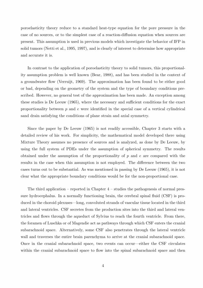
where t is in either seconds or days. The parameters that are fixed are: the tumor radius

R = 0.4 cm, the vascular network density SV = 150 cm−1, being a nominal value of the

range provided in Table 2.1, and the hydraulic conductivity K = 2.5 × 10−7 cm2 second−1

mmHg−1. However, the capillary permeability coefficient Lp increases from the normal tissue

value L0p = 3.6 × 10−8 cm2 second−1 mmHg−1 to the tumor value L∞

p = 1.9 × 10−6 cm2

second−1 mmHg−1. Thus, the value for C is calculated by equation (2.25) to be 50.7.

Figure 2.2, Figure 2.3 and Figure 2.4 show the effect of the frequency D from Table 2.3

on α(t). In all cases, α(t) start with the normal tissue value of α0 = 1.1 and gradually reaches

the tumor value of α∞ = 7.7. The only difference between the three graphs is the time needed

to reach steady state. Figure 2.2, with D1 = 130 second−1, shows that α reaches the carrying

capacity within seconds; however, Figure 2.3 and Figure 2.4, with D2 = 1 day−1 and D1 = 13

day−1 respectively, show that steady state occurs within several days.

0 50 100 150 200 250 3001

2

3

4

5

6

7

8

time (second)

α(t)

D1 = second −1130

Figure 2.2: Behavior of α(t) modeled by Lp(t) with D1 = 130 second−1

25

0 2 4 6 8 101

2

3

4

5

6

7

8

time (day)

α(t)

D2 = 1 day−1

Figure 2.3: Behavior of α(t) modeled by Lp(t) with D2 = 1 day−1

0 5 10 15 20 25 301

2

3

4

5

6

7

8

time (day)

α(t) D3 = day −11

3

Figure 2.4: Behavior of α(t) modeled by Lp(t) with D3 = 13 day−1

26

Evolution of IFP modeled by Lp(t)

The analytic IFP transient solution in full dimensional form is

p(r, t) =2 pv r

R

∞∑n=1

(−1)n+1 sin(nπ rR)

nπβ(t)−1

∫ tT

0

(β(t) α2(t′)

)dt′ + pi, (2.53)

where

β(t) = exp([

α20(1 + C) + (nπ)2

] t

T+

α20C

DT(e−Dt − 1)

). (2.54)

The behavior of α(t) impacts the evolution of IFP within a solid tumor in this model as

seen in Figure 2.5, Figure 2.6 and Figure 2.7. As time elapses, the IFP increases, which is

regulated by α(t) – in particular, by the frequency D – and reaches the tumor steady state

IFP value.

0 50 100 150 200 250 3000

5

10

15

20

time (second)

pres

sure

(mm

Hg)

D1 = second −1

r = 0.2 cm

130

Figure 2.5: Transient IFP profile modeled by Lp(t) with D1 = 130 second−1

27

0 2 4 6 8 100

5

10

15

20

time (day)

pres

sure

(mm

Hg)

D2 = 1 day−1

r = 0.2 cm

Figure 2.6: Transient IFP profile modeled by Lp(t) with D2 = 1 day−1

0 5 10 15 20 25 300

5

10

15

20

time (day)

pres

sure

(mm

Hg)

D3 = day −1

r = 0.2 cm

13

Figure 2.7: Transient IFP profile modeled by Lp(t) with D3 = 13 day−1

28

Evolution of α(t) modeled by SV (t)

The transient behavior of α(t) modeled by SV (t) is simulated using equation (2.27),

α(t) = α0

√1 + E (1 − e−Ft), (2.55)

where t is in days. As in the previous case with Lp(t), the hydraulic conductivity K =

2.5×10−7 cm2 second−1 mmHg−1 is kept constant. The capillary permeability coefficient Lp

increases from the normal tissue value L0p = 3.6 × 10−8 cm second−1 mmHg−1 to the tumor

value L∞p = 1.9 × 10−6 cm second−1 mmHg−1. However, since the vascular density is of

interest, two cases are considered. Given that the range of SV , is the same for both normal

tissue and a solid tumor, 50− 250 cm−1, the normal tissue value SV

0is fixed at 50 cm−1, the

lower extreme. For the tumor value, two SV possibilities are considered: when S

V

∞assumes

150 cm−1, the average of the range, or 250 cm−1, which is the higher extreme. Thus, the

parameter E is calculated from equation (2.29) to be either 154.0 or 257.3, depending on the

tumor value for SV , as shown in Table 2.5. Lastly, the frequency F represents the increase in

the vascular network. The two values examined are for SV increased when the tumor growth

is rapid, F2 = 17 day−1, and when the tumor growth is slow, F4 = 1

16 day−1, as per Table 2.4.

Case Normal tissue Tumor E equation (2.89)

1 SV

0= 50 cm−1 S

V

∞= 150 cm−1 154.0

2 SV

0= 50 cm−1 S

V

∞= 250 cm−1 257.3

Table 2.5: Values for vascular density SV and parameter E

Figure 2.8 and Figure 2.9 illustrate the behavior of α(t) modeled by SV (t) using equation

(2.55). Both figures begin with α0 = 1.1 when SV

0= 50 cm−1 and rise to α∞ = 13.4 when

SV

∞= 150 cm−1, or α∞ = 17.3 when S

V

∞= 250 cm−1. As in the Lp(t) model, the only

difference again is the length of time needed for the steady state to occur. The steady state

is achieved in approximately 10 days with the frequency F2, and 40 days with the frequency

F4.

29

0 20 40 60 800

2

4

6

8

10

12

14

16

18

time (day)

α(t)

Case 1 Case 2

F2 = day −117

Figure 2.8: Behavior of α(t) modeled by SV (t) with F2 = 1

7 day−1

0 50 100 150 2000

2

4

6

8

10

12

14

16

18

time (day)

α(t)

Case 1 Case 2

F4 = day −1116

Figure 2.9: Behavior of α(t) modeled by SV (t) with F4 = 1

16 day−1

30

Evolution of IFP modeled by SV (t)

The analytic IFP transient state solution in full dimensional form is

p(r, t) =2 pv r

R

∞∑n=1

(−1)n+1 sin(nπ rR)

nπψ(t)−1

∫ tT

0

(ψ(t) α2(t′)

)dt′ + pi, (2.56)

where

ψ(t) = exp([

α20(1 + E) + (nπ)2

] t

T+

α20E

FT(e−Ft − 1)

). (2.57)

Similar to the case of IFP modeled by Lp(t), α(t) affects the increase in IFP within a

solid tumor as seen in Figure 2.10 and Figure 2.11. The figure shows how the IFP gradually

increase to its steady state. Again, the rate at which steady state occurs depends on the

frequency F . The smaller the value of the frequency F , the longer the IFP takes to attain

its steady state.

0 20 40 60 800

5

10

15

20

time (day)

pres

sure

(mm

Hg)

Case 1 Case 2

F2 = day −1

r = 0.2 cm

17

Figure 2.10: Evolution of IFP modeled by SV (t) with F2 = 1

7 day−1

31

0 50 100 150 2000

5

10

15

20

time (day)

pres

sure

(mm

Hg)

Case 1 Case 2

F4 = day−1

r = 0.2 cm

116

Figure 2.11: Evolution of IFP modeled by SV (t) with F4 = 1

16 day−1

2.6 Application to anti-angiogenesis therapy

Angiogenesis is one of the hallmarks of cancer. It is a physiological process believed

to be triggered by an imbalance of pro- and anti- angiogenic signals within solid tumors

that creates an abnormal vasculature network characterized by dilated, tortuous and hyper-

permeable capillaries. The consequences of the vascular abnormalities include temporal and

spatial heterogeneity of blood flow and oxygen distribution, decreased levels of oxygen (known

as hypoxia), and increased vascular density, capillary permeability, and increased tumor IFP

within a solid tumor (Goel et al., 2011). This in turn leads to a hostile and chaotic tumor

microenvironment and a significant reduction in the efficacy of cancer therapies, including

radiotherapy and chemotherapy.

Since the discovery of an over-expression of vascular endothelial growth factor (VEGF)

as a contributor to the angiogenic process, clinical efforts have found therapeutic ways to

block the activity of VEGF. The control of VEGF, referred to as anti-VEGF therapy or

anti-angiogenesis therapy, consists of altering the tumor vasculature to resemble the ’normal’

vasculature of normal tissue. This ’vascular normalization’ is characterized by a decrease in

32

the capillary permeability, in vascular density, and in tumor IFP. Vascular normalization also

improves the oxygenation within a solid tumor (Carmeliet and Jain, 2011). The concentration

of oxygen is not incorporated into the models studied in this work and could be of interest

for future research.

The findings of the proposed mathematical model can be extended to possibly assist

experimentalists in their efforts in identifying the optimal time interval to administer anti-

angiogenesis therapy, along with other cancer treatments. This optimal time interval is

defined as the period from the commencement of anti-angiogenesis therapy to the moment

when the normalization effects wear off, following the cessation of the administration of anti-

angiogenesis therapy. This is precisely the window of time during which therapeutic agents,

such as radiation therapy and chemotherapy, can be effectively delivered to possibly prevent

further solid tumor development and metastasis.

Mathematical model for anti-angiogenesis therapy

The anti-angiogenesis therapy mathematical model is similar to the previous models where

the evolution of IFP from a healthy interstitium to a cancerous state was examined. The

PDE (2.21) subject to the boundary conditions (2.22), and under the same assumptions

is employed; however, it is extended to predict the IFP distribution within a solid tumor

due to the effects of anti-angiogenesis therapy. The main feature of the anti-angiogenesis

therapy models is that IFP decreases from the tumor steady-state to the normalized state

and increases from the normalized state to the tumor steady-state either by a change in the

hydraulic permeability of the vascular walls modeled by Lp(t), or in the vascular density

modeled by SV (t).

When analyzing the IFP distribution due to the effects of anti-angiogenesis therapy, three

time intervals are considered, as seen in Table 2.6. Within the three intervals, the continuous

function α2(t) is modeled by either Lp(t) or SV (t) to predict the IFP change due to the various

stages in anti-angiogenesis therapy.

33

Therapy timeline Time interval Description

Pre-therapy 0 ≤ t ≤ t1 IFP evolves from a normal tissuestate at time t = 0 to a tumor state

at time t1

During therapy t1 ≤ t ≤ t2 therapy is administered at time t1and the IFP decreases until time t2

when the effects of the therapy wear off

Post-therapy t2 ≤ t ≤ t3 from time t2 the IFP reboundsback to the tumor state values

at some time t3

Table 2.6: Anti-angiogenesis therapy timeline

Within every time interval the representation of α2(t) changes its form. In the time

intervals between 0 and t1 and between t2 and t3, α2(t) assumes the exponential form as

modeled by Lp(t) (2.23) or by SV (t) (2.27) in full dimensional form as previously elaborated

on. The effects of anti-angiogenesis therapy modeled by either Lp(t) or SV (t) next.

Model of IFP evolution by Lp(t) with anti-angiogenesis therapy

To simulate the effect of anti-angiogenesis, an exponentially decreasing function of time

is considered

α2(t) = P + Qe−Mt, t1 ≤ t ≤ t2, (2.58)

where P , Q and M are constants. The parameters P and Q can be determined the following

way. As anti-angiogenic therapy is applied after the IFP has reached the tumor steady state,

the first condition applied is

α2(t1) = α2∞ =

R2

KL∞

pS

V, (2.59)

and when α2(t) decreases to its minimum at t2, the second condition applied is

α2(t2) = α2N =

R2

KLN

pS

V, (2.60)

where αN is the normalized value of the dimensionless parameter. Thus, the function (2.58)

is calculated to be

α2(t) = α2∞

[1 + J

(e−Mt − e−Mt1

)], t1 ≤ t ≤ t2, (2.61)

34

where the constant J is

J =(

LNp

L∞p

− 1)(

e−Mt2 − e−Mt1)−1

. (2.62)

Value for the frequency parameter M

Since there are three time intervals in the anti-angiogenesis therapy, three different fre-

quencies are needed. In the time interval from 0 to t1, the parameter D (2.29) assumes 1

day−1 for an intermediate growing tumor (Table 2.3). The same frequency value, denoted as

D∗, is used in the interval from t2 to t3. This assumption is based on the fact that it takes

approximately the same amount of time for the IFP to rebound back to its tumor value as

it takes initially starting with a healthy interstitium, since an increase in Lp is a fast process

within a solid tumor (Bates and Curry, 1996).

All that remains now is to determine the parameter M and the endpoints t1 and t2 of the

time interval over which anti-angiogenic therapy is effective. The IFP grows until it reaches

the tumor steady state value and is capped off at time t1 which marks the commencement of

the anti-angiogenesis therapy. From t1 to t2, the parameter M assumes the frequency value

of 13 day−1. It has been observed in human transplanted carcinomas growing in mice that

with a single injection of anti-VEGF treatment DC101 the vascular permeability drops to

approximately 50 percent of its initial value within 3 days (Tong et al., 2004). Furthermore,

the normalization window is short lived – about 6 days (Jain, 2005, 2008). For the purposes

of our model, the transient normalization window runs for approximately 15 days in order to

simulate the effects of anti-VEGF treatment, since Tong et al. (2004) reported that the anti-

VEGF treatment DC101 significantly reduces the tumor IFP even after 15 days. Around day

15, denoted as time t2, the anti-angiogenesis therapy begins to wear off and the IFP begins

to rise up to time t3.

Results of transient IFP modeled by Lp(t) with anti-angiogenesis therapy

The PDE (2.21) with the same boundary conditions (2.22) is integrated with the appro-

priate initial condition in each time interval, and with the appropriate form of the function

α2(t) given by

α2(t) =R2

KLp(t)

S

V, (2.63)

35

where SV is regarded as a parameter in order to gain an insight into how the pressure profile

changes with the vascular surface density. The results are shown in Figure 2.12, where the

IFP profile of the tumor is simulated for three different values of SV – namely the lower

extreme, the average value, and higher extreme, as seen in Table 2.1. The parameters R, K,

L∞p are taken from Table 2.1. The value of normalized hydraulic permeability parameter LN

p ,

3.7× 10−7 cm second−1 mmHg−1, has been taken from Jain et al. (2007). From Figure 2.12,

it is clear that the ”window” of reduced IFP in the middle of the tumor (located 0.2 cm from

the center) is noticeable only for the lower extreme of the vascular density. The IFP barely

decreases for the average value and higher extreme value of SV .

As a sensitivity analysis, Figure 2.13 shows that values of SV lower than 50 cm−1 further

decrease the IFP in the time interval t1 ≤ t ≤ t2. However, when SV is 20 cm−1, 30 cm−1

or 40 cm−1, the corresponding tumor values of α∞ are 4.9, 6.0 and 7.0 at times t1 and t3

which are barely high enough to increase the IFP to a cancerous state according to Jain et al.

(2007). Lastly, Figure 2.14, using SV = 50 cm−1, shows that increasing the frequency value

M only forces the IFP to decrease faster to its steady state within the 15 day normalization

window.

0 5 10 15 20 250

5

10

15

20

time (day)

pres

sure

(mm

Hg)

= 50 cm−1

= 150 cm−1

= 250 cm−1

r = 0.2 cm

SVSVSV

t1 t2 t3

Figure 2.12: Evolution of IFP modeled by Lp(t) with M = 13 day−1

36

0 5 10 15 20 250

5

10

15

20

time (day)

pres

sure

(mm

Hg)

r = 0.2 cm

t1 t2 t3

= 40 cm−1

= 30 cm−1

= 20 cm−1

SVSVSV

Figure 2.13: Evolution of IFP modeled by Lp(t) with SV = 20, 30 and 40 cm−1

0 5 10 15 20 250

5

10

15

20

time (day)

pres

sure

(mm

Hg)

M = 1 day−1

M = day−1

M = day−1

= 50 cm−1

r = 0.2 cm

15

SV

13

t1 t2 t3

Figure 2.14: Evolution of IFP modeled by Lp(t) with M = 1, 13 and 1

5 day−1

37

Model of IFP evolution by SV (t) with anti-angiogenesis therapy

The effect of anti-angiogenesis modeled by SV (t) is formulated again by an exponentially

decreasing function of time

α2(t) = U + V e−St, t1 ≤ t ≤ t2, (2.64)

where U , V and S are constants. The parameters U and V are calculated as follows. As

anti-angiogenic therapy is applied after the IFP has reached the tumor steady state, the first

condition applied is

α2(t1) = α2∞ =

R2

KL∞

pS

V

∞, (2.65)

and when α2(t) decreases to its minimum at t2, the second condition applied is

α2(t2) = α2N =

R2

KLN

pS

V

N

, (2.66)

where SV

Nis the normalized value of the vascular density. Thus, the function (2.64) is

calculated to be

α2(t) = α2∞

[1 + X

(e−St − e−St1

)], t1 ≤ t ≤ t2, (2.67)

where the constant X is

X =(

LNp

SV

N

L∞p

SV

∞ − 1)(

e−St2 − e−St1)−1

. (2.68)

Value for the frequency parameter S

In the time interval from 0 to t1, the parameter F (2.29) assumes F2 = 17 day−1 for a

fast growing tumor with increased SV from Table 2.4. The same frequency values, denoted as

F ∗2 , are used in the interval from t2 to t3. This is based on the assumption that the vascular

density would increase after anti-angiogenesis therapy at the same frequency as it did in the

case of an increase from a healthy interstitium to a cancerous state.

The frequency parameter S and the endpoints t1 and t2 of the time interval over which

anti-angiogenic therapy is effective are determined in the following way. Once the IFP

reaches its tumor steady state, it is capped off at t1, marking the commencement of the

anti-angiogenesis therapy. From t1 to t2, the parameter S assumes the frequency value of15 day−1. Tong et al. (2004) reported that, in human transplanted carcinomas growing in

38

mice, within 2 − 3 days after a single injection of DC101 many of the vessels become less

tortuous besides being smaller in diameter, and by day 5, in some regions of the tumor, some

of the vessels regressed completely. The effects on the IFP due to a ’normalized’ vasculature

are again simulated for approximately 15 days. Around day 15, denoted as time t2, the IFP

decrease is stopped, which represents the loss of the effects of DC101. From then on, the IFP

rebounds to a tumor state value at time t3.

Results of transient IFP modeled by SV (t) with anti-angiogenesis therapy

The evolution of IFP due to anti-angiogenesis therapy modeled by SV (t) is approached

differently compared to the previous case. Clinical studies have shown that anti-angiogenesis

therapy prunes the newly formed blood vessels and shrinks and decreases the permeability

of the pre-existing capillaries (Carmeliet and Jain, 2011). Thus, the parameter SV is not kept

constant, but rather changes. Again, the PDE (2.21) with the same boundary conditions

(2.22) is integrated with the appropriate initial condition in each time interval and with the

appropriate form of the function α2(t).

Under the normal tissue state and the vascular normalization process, SV assumes the

lower extreme value of 50 cm−1. The vascular normalization is characterized by the range

50−250 cm−1 for the values of SV , according to Jain et al. (2007); however, any value greater

than 50 cm−1 results in a value of αN close to tumor α∞ value which does not effectively

decrease the IFP. Furthermore, in modeling by SV (t), when a tumor attains tumor values

at time t1 and t3, SV is either 150 cm−1, which is the average value, or 250 cm−1, which is

the higher extreme. The changes in vascular density SV within the anti-angiogenesis therapy

timeline are summarized in two cases in Table 2.7.

Time interval Case A Case B

0 ≤ t ≤ t1 normal tissue → tumor normal tissue → tumorSV

0= 50 cm−1 → S

V

∞= 150 cm−1 S

V

0= 50 cm−1 → S

V

∞= 250 cm−1

t1 ≤ t ≤ t2 tumor → normalized tumor → normalizedSV

∞= 150 cm−1 → S

V

N= 50 cm−1 S

V

∞= 250 cm−1 → S

V

N= 50 cm−1

t2 ≤ t ≤ t3 normalized → tumor normalized → tumorSV

N= 50 cm−1 → S

V

∞= 150 cm−1 S

V

N= 50 cm−1 → S

V

∞= 250 cm−1

Table 2.7: Values for vascular density SV in anti-angiogenesis therapy timeline

39

In conjunction with SV changing, the value for Lp needs to represent the state of the

tumor in the model as well. Thus, the values of L0p and L∞

p are taken from Table 2.1, and

the normalized LNp is 3.7 × 10−7 cm second−1 mmHg−1 (Jain et al., 2007). Lastly, R and K

are kept constant, and their respective values can be found in Table 2.1.

In the middle of the tumor (located 0.2 cm from the center), Figure 2.15 shows a 25%

drop in IFP in the time interval t1 ≤ t ≤ t2 for both Case A and Case B from Table 2.7.

In Figure 2.16, if the normalized SV

Nis less than 50 cm−1 at time t2, while the tumor S

V

∞

assumes the average value of 150 cm−1 at times t1 and t3, the IFP drops approximately 35%

– nowhere near the IFP for a healthy interstitium. Again, considering Case A for the change

in SV in Table 2.7, a decrease in the frequency S in the time interval t1 ≤ t ≤ t2 only delays

the IFP in reaching its steady state, as seen in Figure 2.17.

0 10 20 30 500

5

10

15

20

time (day)

pres

sure

(mm

Hg)

Case A Case B

S = day−1

r = 0.2 cm

t1 t2 t3

15

Figure 2.15: Evolution of IFP modeled by SV (t) with S = 1

5 day−1

40

0 10 20 30 500

5

10

15

20

time (day)

pres

sure

(mm

Hg)

S = day −1

r = 0.2 cm

t1 t2 t3

= 40 cm−1

= 30 cm −1

= 20 cm−1

SVSVSV15

N

N

N

Figure 2.16: Evolution of IFP modeled by SV (t) with S

V

N= 20, 30 and 40 cm−1

0 10 20 30 500

5

10

15

20

time (day)

pres

sure

(mm

Hg)

Case A r = 0.2 cm

t1 t2 t3

S = day−1

S = day −1

S = day−117

15

13

Figure 2.17: Evolution of IFP modeled by SV (t) with S = 1

3 ,15 and 1

7 day−1

41

From both models which describe the rise of IFP from normal tissue values to tumor

tissues values and the application to anti-angiogenesis therapy, it is clear that the capillary

permeability Lp has a greater effect on the tumor IFP than the vascular density SV . In the

case of the evolution of IFP modeled by Lp(t) from normal tissue values to tumor values,

Lp depends on the tumor growth rate and drastically influences the IFP, as seen in Figures

2.5-2.7. Modeling by SV (t), the IFP reaches tumor steady state roughly at the same time

independent of the type of tumor growth which shows that vascular density may not be an

important contributor to the IFP evolution. Similar behavior of Lp and SV are also seen in

the model which incorporates the effects of anti-angiogenesis therapy. The model of IFP

evolution by Lp(t) shows that the decrease in IFP was influenced highly by the tumor growth

rate, as seen in Figure 2.14. Whereby having different values of SV , which were kept constants,

also influenced the amount of IFP decrease within a solid tumor, as seen in Figure 2.12.

However, modeling S/V as a time dependent function appears to have the same impact on

the decrease in IFP independent of the actual change in S/V, as seen in Figure 2.15, and of

the tumour growth rate as in Figure 2.17. Thus, from a clinical perspective, according to

these models which incorporate anti-angiogenesis therapy, the primary parameter to focus

on is the capillary permeability Lp, which highly influences the IFP change within a tumor.

The models also predict that the optimal time for anti-angiogenesis therapy in conjunction

with other cancer treatments such as radiotherapy and chemotherapy would be after time

t1 and before t2. Note that these models are very crude and only focus on the changes in

capillary permeability and vascular density. Within a solid tumor, there are other changes

in the microenviroment that occur such as hypoxia and acidosis which are not accounted for

and may be of importance to consider.

42

Chapter 3

Testing the approximation (2μ + λ)e(r, t) = p(r, t) in a hollowspherically symmetric domain

3.1 Introduction

As seen in Chapter 2, the mathematical model adopted in this Thesis is built on two

partial differential equations. The first equation is the continuity equation with field variables

which depend on both space r = (x, y, z) in centimeters and time t in seconds:

∂e

∂t− K∇2p =

LpS

V(pv − p), (3.1)

where e(r, t) is the tissue dilatation being the change of volume per unit volume of both the

fluid and the solid phase together, K is the hydraulic conductivity coefficient (with units

cm2 second−1 mmHg−1), Lp is the permeability of the capillary walls with (units in cm

second−1 mmHg−1), and SV is the surface area per unit volume of blood vessels (with units

cm−1). All pressure quantities are measured in mmHg. The variable p(r, t) is the interstitial

fluid pressure (IFP) and pv is the microvascular pressure. The second equation contains the

relation between e and p which is derived in Appendix A, equation (A28), namely

(2μ + λ)∇2e = ∇2p, (3.2)

where μ and λ are the Lame parameters for elasticity of a solid material (with units mmHg).

It is evident that equation (3.1) alone is not closed, and thus, equation (3.2) is needed. As

mentioned in Chapter 2 and Appendix A, there is a special case in which equation (3.2)

implies a linear relation between e and p, namely

(2μ + λ)e = p. (3.3)

To summarize the argument, equation (3.2) may be rewritten as

∇2(p − (2μ + λ)e) = 0, (3.4)

43

which is equivalent to ⎧⎪⎨⎪⎩

p − (2μ + λ)e = f(r, t),

∇2f = 0,(3.5)

where f(r, t) is an unknown harmonic function. Only in the case when f is identically zero,

the combination of equations (3.1) and (3.5) gives

12μ + λ

∂p

∂t− K∇2p =

LpS

V(pv − p), (3.6)

which is the PDE for the IFP used in Chapter 2.

Taking f ≡ 0 in equation (3.5) is a special case which appears in many places in the

ground water flow literature (Bear, 1988). It holds in the one-dimensional case when the

fluid flow as well as deformations occur in one direction only, as discussed in Verruijt (1969).

Also, f ≡ 0 is valid in the three-dimensional case, assuming that the radial displacements

vanish identically. However, in the present context, it is difficult to justify physically such an

assumption. Furthermore, after investigating the relation between e and p in more detail in

spherical coordinates under the assumption of radial symmetry, it appears that taking f to

be identically zero is questionable; for, as shown in Appendix B, even in the simplest case of

spherical symmetry, the function f(r, t) does not vanish, but remains as an arbitrary function

of time,

f = b(t). (3.7)

This form of f still leaves two unknown variables in equation (3.1),

12μ + λ

(∂p

∂t− ∂b(t)

∂t

)− K∇2p =

LpS

V(pv − p), (3.8)

and so even in the simplest case of spherical symmetry the condition ∂b∂t = 0 needs to be

satisfied for the pressure to obey equation (3.6). De Leeuw (1965) first found the necessary

and sufficient conditions on f by considering a hollow cylindrical sand drain under the as-

sumptions of axial symmetry and plane strain. Using Biot’s equations of the linear theory of

poroelasticity (1941) and assuming that the fluid is incompressible, De Leeuw described the

three-dimensional system by two equations, both depending on space r and time t, which in

his notation and coordinate-independent form are as follows:

k

γw∇2u =

∂e

∂t, (3.9)

44

where k is the permeability, γw is the unit weight of water, u is water pressure, and e is the

volume dilatation; the second equation reads

(K +43G)∇2e = ∇2u, (3.10)

where K is the compressibility modulus and G is the shear modulus of the solid constituent.

By expressing equation (3.10) in cylindrical coordinates r, θ, and z, and integrating, it

follows that

(K +43G)e = u + g(r, θ, z, t), (3.11)

where g must satisfy ∇2g = 0. Under the assumption of axial symmetry and plane strain,

that is, ∂∂θ = 0 and ∂

∂z = 0, except for ∂uz∂z = constant, one finds

(K +43G)e = u + g(t), (3.12)

where now g depends solely on time. Taking the derivative of equation (3.12) with respect

to t and substituting into equation (3.9) yields

k

γw∇2u =

1K + 4

3G

(∂u

∂t+

∂g

∂t

), (3.13)

which gives a ”heat-type” equation when ∂g∂t = 0. De Leeuw then goes on to show that for

the sand drain problem appropriate boundary conditions need to be considered in order to

make ∂g∂t precisely zero; consequently, the hydraulic pressure and the dilatation are exactly

proportional in that case.

3.1.1 Some details of De Leeuw (1965) argument

De Leeuw is careful to point out that this result is not generally valid, and it certainly

does not hold in spherical coordinates. However, in most of the porous media literature, as

well as in Chapter 2, the assumption that e and p are proportional has been used; hence, given

that the condition g = 0 is only an approximation, the question that needs to be answered

is: how good an approximation is it?

In order to test this assumption, and therefore answer the question, a review of the De

Leeuw (1965) paper in more detail is needed so as to see how the geometry - and hence the

boundary conditions - affect the problem. De Leeuw solved the system of PDEs (3.9) and

45

(3.10) for a vertical sand drain consisting of a hollow cylindrical body as sketched in the

figure below,

xy

z

z=h

z=0

Rρ

Figure 3.1: Hollow cylindrical domain

with the following boundary conditions

0 < z < h, r = R, ur = f1(t), (3.14)

0 < z < h, r = ρ, ur = f2(t), (3.15)

z = h, ρ < r < R, pv = f3(t), (3.16)

0 < z < h, r = ρ, u = f4(t), (3.17)

0 < z < h, r = R,∂u

∂r= 0, (3.18)

z = 0 and z = h, 0 < r < R,∂u

∂z= 0, (3.19)

where h is the height of the cylinder, ρ and R are the inner and outer radii of the cylinder,

and pv is the applied load. The coordinate system is cylindrical, and plane strain and axial

symmetry are assumed. The functions of time fi(t), where i = 1, 2, 3, 4, are arbitrary. Note

that the notation of De Leeuw is a bit confusing since ur is radial displacement while u is the

hydraulic pressure.

Using the Laplace transform, De Leeuw found the general solution of the two coupled

PDEs, that is, he found the transformed quantities e(r, s) and u(r, s). Finally, taking advan-

tage of the equation of motion, applying the transformed boundary conditions, and inverting

46

the Laplace transform, De Leeuw was able to show that the function g in equation (3.12)

must satisfy the following condition:

∂g

∂t= − ∂

∂t

[4GRρ

R2 − ρ2

(f1

ρ− f2

R

)+ f3 + 2f4

]. (3.20)

It is clear that in cylindrical geometry, with plane strain and axial symmetry, and with the

special boundary conditions

f1 = f2 = f4 = 0, f3 = pv = constant, (3.21)

the harmonic function g is a constant, which can be taken to be zero. This makes the volume

dilatation e proportional to the hydrostatic pressure u. Also, it is obvious from equation

(3.20) that this proportionality does not exist if even one of the functions fi depends on time.

3.1.2 The case of a spherically symmetric sand drain

In order to simplify the mathematical analysis, De Leeuw (1965) considered the case

of consolidation in the absence of sources. Therefore, for the same reason, the right-hand

side of equation (3.1) is set to zero and equation (3.2) is kept unchanged. For the reader’s

convenience, these equations are repeated below:

∂e

∂t=

κ

η∇2p, (3.22)

where the hydraulic conductivity has been expressed in terms of the permeability κ and the

viscosity η, and

(2μ + λ)∇2e = ∇2p, (3.23)

which is equivalent to ⎧⎪⎨⎪⎩

p − (2μ + λ)e = f(r, t),

∇2f = 0.(3.24)

Now, if f(r, t) ≡ 0, then equation (3.22) becomes

∂p

∂t= γ∇2p, (3.25)

where γ = κη (2μ+λ), and the problem is reduced to a ”heat-type” equation for the hydraulic

pressure.

The enormous mathematical simplification resulting from this kind of argument repre-

sents explains the popularity of the assumption of proportionality of hydraulic pressure and

47

dilatation. The analysis is far more complicated in the general case, for as pointed out already

by Verrujit (1969), the solution of the basic PDEs (3.22) and (3.23) is not enough, since the

boundary conditions for the elastic material are given in terms of stresses or displacements –

not in terms of dilatation. Therefore, after obtaining the general solution for e(r, t) = ∇ · uand p(r, t) from equations (3.22) and (3.23), the equation of motion is employed in order to

solve for u(r, t), namely

μ∇2u + (μ + λ)∇e = ∇p, (3.26)

where the boundary conditions can be enforced. This problem is far more difficult than solving

the ”heat-type” equation (3.25) with a constant initial condition and constant boundary

conditions.

Going back to the question raised earlier - namely, how good an approximation f(r, t) ≡ 0

is in the case of a homogeneous, spherically symmetric domain - a test can be constructed as

follows:

1. Solve equation (3.25) with appropriate initial and boundary conditions;

2. Find the general solution of the system of PDEs (3.22) and (3.23) to get the general form

of e(r, t) and p(r, t);

3. Substitute these into equation (3.26) and solve for u(r, t) with the same boundary condi-

tions as in Step 1, and thus, calculate the stress tensor, and hence, the pressure.

4. Compare the hydraulic pressure values obtained in Step 1 and Step 3.

3.2 Step 1: Approximated case

Equation (3.25) from Section 3.1 which is analogous to the heat equation is solved ana-

lytically with appropriate initial and boundary conditions.

Since the interest is to study the pressure behavior within a sphere with a hollow spherical

center as shown in Figure 3.2, the PDE (3.25) is rewritten in spherical coordinates, assuming

radial symmetry:

∂p(r, t)∂t

= γ

(2r

∂p(r, t)∂r

+∂2p(r, t)

∂r2

). (3.27)

48

The boundary conditions imposed on equation (3.27) are analogous to those in De Leeuw

(1965) paper for a cylindrical body with a cylindrical hollow center for the sand drain problem,

namely ⎧⎪⎨⎪⎩

p(ri, t) = f1(t),p(ro, t) = f2(t),p(r, 0) = 0,

(3.28)

where ri and ro are the inner and outer radii of the sphere, and f1(t) and f2(t) are arbitrary

functions of time. Note that in this case no boundary conditions need to be prescribed for

the stresses; hence, there is no need to bring in explicitly the equation of motion (3.26).

xy

z

riro

Figure 3.2: Hollow spherical domain

This boundary value problem is solved by applying the Laplace transform:

P (r, s) =∫ ∞

0p(r, t) exp(−st)dt. (3.29)

The PDE (3.27) and the boundary conditions are transformed as:

d2P

dr2+

2r

dP

dr− s

γP = 0 (3.30)

with ⎧⎪⎨⎪⎩

P (ri, s) = F1(s),

P (ro, s) = F2(s).(3.31)

The initial condition P (r, 0) = 0 was used in deriving equation (3.30).

49

To proceed in solving the differential equation (3.30), a change of variable is applied. Let

P = y(r,s)r . Then, dP

dr = y′r−yr2 and d2P

dr2 = y′′

r − 2 y′

r2 + 2yr3 , and equation (3.30) reads(

y′′

r− 2

y′

r2+

2y

r3

)+

2r

(y′r − y

r2

)− s

γ

y

r= 0, (3.32)

which reduces to

y′′ − s

γy = 0. (3.33)

The characteristic equation, q2 − sγ = 0, gives q = ±

√sγ . Thus, the general solution is

y = c1(s)e

√sγ r

+ c2(s)e−√

sγ r

, (3.34)

where c1(s) and c2(s) are so far arbitrary functions of s. The solution (3.34) can be written

in the form

y = M(s) sinh(√

s

γr) + N(s) cosh(

√s

γr), (3.35)

where M(s) and N(s) are arbitrary functions of s. This form is extremely valuable in applying

the inverse Laplace transform later in the calculations. Thus,

P (r, s) =M(s)

rsinh(

√s

γr) +

N(s)r

cosh(√

s

γr). (3.36)

Now, the Laplace transformed boundary conditions (3.31) are used to find M(s) and

N(s). Equations (3.31) and (3.36) yield

F1(s) =M(s)

risinh(

√s

γri) +

N(s)ri

cosh(√

s

γri) (3.37)

and

F2(s) =M(s)

rosinh(

√s

γro) +

N(s)ro

cosh(√

s

γro). (3.38)

Solving this linear system for M(s) and N(s), one obtains

M(s) =riF1(s) cosh(

√sγ ro) − roF2(s) cosh(

√sγ ri)

sinh(√

sγ (ro − ri))

. (3.39)

and

N(s) =riF1(s) sinh(

√sγ ro) − roF2(s) sinh(

√sγri)

sinh(√

sγ (ro − ri))

. (3.40)

50

The hyperbolic identity sinh(x− y) = sinh(x) cosh(y)− cosh(x) sinh(y) has been used several

times to simplify M(s) and N(s), as well as the final result. Substituting equations (3.39)

and (3.40) into (3.36) yields

P (r, s) =riF1(s) sinh(

√sγ (ro − r)) + roF2(s) sinh(

√sγ (r − ri))

r sinh(√

sγ (ro − ri))

. (3.41)

Before the inverse Laplace transform can be applied to equation (3.41), F1(s) and F2(s)

cannot be left as arbitrary functions of s. Thus, in light of De Leeuw (1965) sand drain

problem, the boundary conditions f1(t) and f2(t) are assumed to be constants:{f1(t) = α,f2(t) = β,

(3.42)

where α < β. Their Laplace transforms are{F1(s) = α

s ,

F2(s) = βs .

(3.43)

Thus, the solution of the approximated case (3.41) reads

P (r, s) =riα sinh(

√sγ (ro − r)) + roβ sinh(

√sγ (r − ri))

rs sinh(√

sγ (ro − ri))

. (3.44)

The inversion of the Laplace-transformed solution (3.44) is straightforward, and is re-

ported, for completeness, in Appendix C. However, it is unlikely that such an inversion can

be made in the test case problem formulated at the end of Section 3.1, namely the calculation

of the pressure p when it is not assumed to be proportional to the dilatation e. Consequently,

it is the above solution for P (r, s) that is compared with its analogous expression in the second

problem. This is clearly legitimate since - as it is well known - for continuous functions of at

most exponential order the original function p(r, t) is mapped uniquely into the transformed

function P (r, s) (D.V. Widder, Advanced Calculus, Chapter 13, Dover 1989). In short, the

goodness of the approximation in question can be assessed in terms of the frequency domain

as well as in the terms of the time domain.

3.3 Steps 2 and 3: Test case

In this Section, the general solution of the system of PDEs (3.22) and (3.23) from Section

3.1 is computed in order to get the general form of e(r, t) and p(r, t). Then, these quantities are

51

substituted into equation (3.26) which is solved for u(r, t) with the same boundary conditions

as in Section 3.2. Note that the calculations and the final solution will be in modified spherical

Bessel function form. This is primarily done for convenience, otherwise the expressions would

be very long. However, one can take the modified spherical Bessel function form of the final

solution and convert it into hyperbolic functions sinh and cosh, as done in Appendix D

equation (D30).

To test the approximation made in Section 3.2, the same system of PDEs is considered:

∂e(r, t)∂t

=κ

η∇2p(r, t), (3.45)

and

(2μ + λ)∇2e(r, t) = ∇2p(r, t). (3.46)

The first equation is known as the storage equation in groundwater flow literature. The

second equation is obtained by taking the divergence of the equation of motion

μ∇2u(r, t) + (μ + λ)∇e(r, t) = ∇p(r, t), (3.47)

and by using the relation e = ∇ · u.

The general solution to the above system is found in the following manner. Equation

(3.46) is substituted into equation (3.45):

∂e

∂t= γ∇2e, (3.48)

where γ = κη (2μ+λ). Since the domain of the problem is a homogeneous, radially symmetric

hollow sphere, equation (3.48) is converted into spherical coordinates:

∂e

∂t= γ

[1r2

∂

∂r

(r2∂e

∂r

)]. (3.49)

Using the Laplace transform,

E(r, s) =∫ ∞

0e(r, t) exp(−st)dt, (3.50)

the PDE (3.49) is rewritten as:

sE(r, s) = γ

[1r2

d

dr

(r2dE(r, s)

dr

)], (3.51)

52

under the assumption that e(r, 0) = 0. Now, viewing s as a constant, the differential equation

(3.51) is rearranged as

d2E

dr2+

2r

dE

dr− s

γE = 0. (3.52)

Recognizing that equation (3.52) is the same as to equation (3.30) in Section 3.2, the

method used in solving equation (3.30) can be employed on equation (3.52) to arrive at the

same general solution (3.39) in terms of hyperbolic functions sinh and cosh. However, unlike

in Section 3.2, where the quantity being solved for was pressure p(r, t), it is not possible to

impose boundary conditions on the volume dilatation e = ΔVV , which is neither a force nor

a stress quantity. This particular issue has been brought up in Chapter 2 and has been well

known in groundwater flow studies as reviewed in Verruijt (1969). Thus, e is expressed in

terms of the solid displacement vector u, since the two are directly related via e = ∇·u. Once

this is accomplished, boundary conditions can be imposed on the system in terms of stress

and strain which can be defined in terms of displacement ur.

To avoid cumbersome calculations, it is convenient to apply the change of variable,

q =√

s

γr, (3.53)

to equation (3.52) which results in the equation(s

γ

)d2E

dq2+

2q

√s

γ

√s

γ

dE

dq− s

γE = 0, (3.54)

or more simply

d2E

dq2+

2q

dE

dq− E = 0. (3.55)

Equation (3.55) is identified as the modified spherical Bessel equation of order zero. The

general solution is (Abramowitz and Stegun (1964), Chapter 10)

E(q, s) =√

π

2q

[A(s)I 1

2(q) + B(s)I− 1

2(q)

], (3.56)

where A(s) and B(s) are arbitrary constants of integration, and√

π2q I 1

2(q) = sinh(q)

q and√π2qI− 1

2(q) = cosh(q)

q are the spherical Bessel functions.

Having a general solution for E(q, s), the next step is to obtain a general solution for

P (q, s), which is the Laplace transformed pressure p(r, t) together with the variable change

53

(3.53). As discussed in Appendix B, equation (3.46) is equivalent to

p(r, t) − (2μ + λ)e(r, t) = g(t), (3.57)

with ∇2g(t) = 0. The Laplace transforms

P (r, s) =∫ ∞

0p(r, t) exp(−st)dt (3.58)

and

G(s) =∫ ∞

0g(t) exp(−st)dt, (3.59)

and the variable change (3.53) give

P (q, s) − (2μ + λ)E(q, s) = G(s), (3.60)

where ∇2G(s) = 0. From equations (3.56) and (3.60), it follows that

P (q, s) = (2μ + λ)√

π

2q

[A(s)I 1

2(q) + B(s)I− 1

2(q)

]+ G(s). (3.61)

Equation (3.61) is used later in this calculation.

From the equation of motion (3.47), the Terzaghi stress tensor is obtained (see Appendix

A). In the geometry of this model, it has only one non-zero component:

τrr(r, t) = λe + 2μerr = λe + 2μ∂ur

∂r, (3.62)

where err is the strain component and u = (ur, 0, 0) is the displacement in the r direction (due

to the assumption of radial symmetry, the second and third components are set to zero). By

means of the Laplace transform and the change of variable (3.53), equation (3.62) is written

as

τrr(q, s) = λE(q, s) + 2μdUr(q, s)

dq

√s

γ. (3.63)

This shows that the term dUrdq needs to be found. Now, note that the volume dilatation e is

defined as

e = err + eθθ + eφφ, (3.64)

where err = ∂ur∂r , eθθ = ur

r , and eφφ = urr are displacement-strain components in the r, θ and

φ directions for a sphere under the assumption of radial symmetry. The Laplace transformed

equation (3.64) yields

E(r, s) =dUr

dr+

Ur

r+

Ur

r=

1r2

d

dr(r2Ur), (3.65)

54

and then under the variable change (3.53)

E(q, s) =√

s

γ

1q2

d

dq(q2Ur). (3.66)

Combining with equation (3.56), it follows that√s

γ

1q2

d

dq(q2Ur) =

√π

2q

[A(s)I 1

2(q) + B(s)I− 1

2(q)

]. (3.67)

By integrating,

q2Ur =√

γ

s

⎡⎢⎢⎢⎢⎢⎣A(s)

∫q2

√π

2qI 1

2(q)dq

︸ ︷︷ ︸J1

+B(s)∫

q2

√π

2qI− 1

2(q)dq

︸ ︷︷ ︸J2

⎤⎥⎥⎥⎥⎥⎦ + C(s), (3.68)

where C(s) is an arbitrary constant of integration. As is well known, the differentiation

formulas for the spherical Bessel functions give:

d

dq

[q2

√π

2qI− 3

2

]= q2

√π

2qI− 1

2(q), (3.69)

and

1q

d

dq

[q2

√π

2qI 3

2

]= q

√π

2qI 1

2(q), (3.70)

(see Abramowitz and Stegun (1964), Formulas 10.2.22 and 10.2.23). These relations are useful

in evaluating the integrals that appear in equation (3.68):

J1 =∫

qq

√π

2qI 1

2(q)dq =

∫q1q

d

dq

[q2

√π

2qI 3

2

]dq = q2

√π

2qI 3

2(q), (3.71)

and

J2 =∫

q2

√π

2qI− 1

2(q)dq =

∫d

dq

[q2

√π

2qI− 3

2

]dq = q2

√π

2qI− 3

2(q). (3.72)

Substituting equations (3.71) and (3.72) into (3.68) leads to

q2Ur =√

γ

s

[A(s)q2

√π

2qI 3

2(q) + B(s)q2

√π

2qI− 3

2(q)

]+ C(s), (3.73)

which simplifies to

Ur =√

γ

s

[A(s)

√π

2qI 3

2(q) + B(s)

√π

2qI− 3

2(q)

]+

C(s)q2

. (3.74)

55

Given that Ur is found, dUrdq is calculated to be

dUr

dq=

√γ

s

[A(s)

d

dq

(√π

2qI 3

2(q)

)+ B(s)

d

dq

(√π

2qI− 3

2(q)

)]− 2

C(s)q3

=√

γ

s

[A(s)

√π

2q

(I 1

2(q) − 2

qI 3

2(q)

)+ B(s)

√π

2q

(I− 5

2(q) +

1qI− 3

2(q)

)]− 2

C(s)q3

.

(3.75)

Furthermore, it is easy to show that

d

dq

(√π

2qI 3

2(q)

)=

√π

2qI 1

2(q) − 2

q

√π

2qI 3

2(q), (3.76)

and,

d

dq

(√π

2qI− 3

2(q)

)=

√π

2qI− 5

2(q) +

1q

√π

2qI− 3

2(q). (3.77)

Consequently, equation (3.63) with the assistance of (3.56) takes on the form

τrr(q, s) = λ

√π

2q

[A(s)I 1

2(q) + B(s)I− 1

2(q)

]

+ 2μ

√s

γ

(√γ

s

√π

2q

[A(s)

(I 1

2(q) − 2

qI 3

2(q)

)+ B(s)

(I− 5

2(q) +

1qI− 3

2(q)

)]− 2

C(s)q3

),

(3.78)

or in simplified form

τrr(q, s) = λ

√π

2q

[A(s)I 1

2(q) + B(s)I− 1

2(q)

]

+ 2μ

√π

2q

[A(s)

(I 1

2(q) − 2

qI 3

2(q)

)+ B(s)

(I− 5

2(q) +

1qI− 3

2(q)

)]− 4μ

√s

γ

C(s)q3

.

(3.79)

For the comparison to the solution (3.44) of the approximated case in Section 3.2, the

pressure needs to be computed. It is given by equation (3.61); however, the values of the

arbitrary constants of integration A(s), B(s) and G(s) need to be found, which requires the

application of boundary conditions. For obvious reasons these boundary conditions need to

be the same as in Section 3.2. Thus, ⎧⎪⎨⎪⎩

p(ri, t) = α,

p(ro, t) = β,(3.80)

56

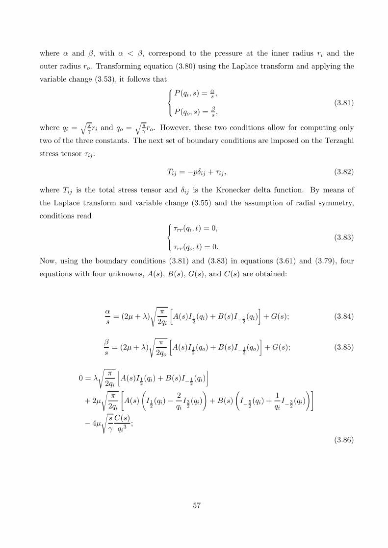
where α and β, with α < β, correspond to the pressure at the inner radius ri and the

outer radius ro. Transforming equation (3.80) using the Laplace transform and applying the

variable change (3.53), it follows that⎧⎪⎨⎪⎩

P (qi, s) = αs ,

P (qo, s) = βs ,

(3.81)

where qi =√

sγ ri and qo =

√sγro. However, these two conditions allow for computing only

two of the three constants. The next set of boundary conditions are imposed on the Terzaghi

stress tensor τij :

Tij = −pδij + τij , (3.82)

where Tij is the total stress tensor and δij is the Kronecker delta function. By means of

the Laplace transform and variable change (3.55) and the assumption of radial symmetry,

conditions read ⎧⎪⎨⎪⎩

τrr(qi, t) = 0,

τrr(qo, t) = 0.(3.83)

Now, using the boundary conditions (3.81) and (3.83) in equations (3.61) and (3.79), four

equations with four unknowns, A(s), B(s), G(s), and C(s) are obtained:

α

s= (2μ + λ)

√π

2qi

[A(s)I 1

2(qi) + B(s)I− 1

2(qi)

]+ G(s); (3.84)

β

s= (2μ + λ)

√π

2qo

[A(s)I 1

2(qo) + B(s)I− 1

2(qo)

]+ G(s); (3.85)

0 = λ

√π

2qi

[A(s)I 1

2(qi) + B(s)I− 1

2(qi)

]

+ 2μ

√π

2qi

[A(s)

(I 1

2(qi) −

2qi

I 32(qi)

)+ B(s)

(I− 5

2(qi) +

1qi

I− 32(qi)

)]

− 4μ

√s

γ

C(s)qi

3;

(3.86)

57

0 = λ

√π

2qo

[A(s)I 1

2(qo) + B(s)I− 1

2(qo)

]

+ 2μ

√π

2qo

[A(s)

(I 1

2(qo) −

2qo

I 32(qo)

)+ B(s)

(I− 5

2(qo) +

1qo

I− 32(qo)

)]

− 4μ

√s

γ

C(s)qo

3.

(3.87)

In Appendix D, the values for A(s), B(s) and G(s) are found (C(s) is not needed).

Once the smoke clears in Appendix D, equation (3.61) becomes

P (q, s) = (2μ + λ)√

π

2q

[A(s)

sI 1

2(q) +

B(s)s

I− 12(q)

]+

G(s)s

, (3.88)

where the over-barred quantities are defined in Appendix D (Equations D21-D23). Returning

back to r via relation (3.53), the solution for the test case is

P (r, s) = (2μ + λ)

√π

2r

√γ

s

[A(s)

sI 1

2(r

√s

γ) +

B(s)s

I− 12(r

√s

γ)]

+G(s)

s. (3.89)

As anticipated at the end of Section 3.2, the inversion of the Laplace transformed pressure

(3.89) is far from trivial; however, it is not necessary, as explained earlier. It is possible to

work directly with the pressure expressed in the frequency domain.

3.4 Step 4: Comparison

In this Section, the Laplace transformed expressions are compared for both the approxi-

mated case and the test case.

58

3.4.1 Parameters

Three different hollow spheres which are considered are shown in Table 3.1.

Sphere Inner radius ri (cm) Outer radius ro (cm) Location r (cm)

1 0.2 0.5 0.35

2 0.5 1 0.75

3 5 10 7.5

Table 3.1: Hollow sphere radii values

Hollow spheres 1 and 2 are close to the size of a tumor, as reported in literature (Jain and

Baxter, 1988; Jain et al., 2007; Lunt et al., 2008). Hollow sphere 3 is more relevant for the

study of ground water flow, where the size of an aquifer can range from centimeters to meters

(Verruijt, 1970; Bear and Verruijt, 1987). To study the pressure behavior for each hollow

sphere, a location r is selected halfway between the inner radius ri and the outer radius ro.

At locations near the inner and the outer radii, the pressure is dominated by the boundary

conditions, and is therefore not considered.

The value of the parameter γ = κη (2μ+λ) is based on the following values. Since κ

η is the

hydraulic conductivity K, it is assigned the value of 2.5× 10−7 cm2 second−1 mmHg−1 (Jain

et al., 2007) as in Chapter 2, for consistency. The Lame elastic parameters μ and λ take on

the values for soft saturated clay from Chapter 2, that is, 3.6 × 104 mmHg and 1.5 × 105

mmHg (Bowles, 1988), respectively. Thus, the value of γ is approximately 0.06 mmHg.

The boundary conditions are selected to be α = 5 mmHg for the inner radius and β = 30

mmHg for the outer radius. These values are reasonable for biological tissue and are selected

to test the approximated case against the test case.

3.4.2 Results

Here, the Laplace transformed solutions for the approximated case,

P (r, s) =riα sinh(

√sγ (ro − r)) + roβ sinh(

√sγ (r − ri))

rs sinh(√

sγ (ro − ri))

, (3.90)

59

and for the test case,

P (r, s) = (2μ + λ)

√π

2r

√γ

s

[A(s)

sI 1

2(r

√s

γ) +

B(s)s

I− 12(r

√s

γ)]

+G(s)

s, (3.91)

are simulated. Note that equation (3.91) is written in modified spherical Bessel form for

convenience and can be converted into hyperbolic functions sinh and cosh as in Appendix D,

equation (D30).

Figure 3.3, Figure 3.4 and Figure 3.5 clearly show that there is a significant enough

difference between the two solutions. In fact, as the inner and the outer radii increase,

the pressure difference between the approximated case and the test case grows larger. This

pressure difference cannot be ascribed to the boundary conditions, as their effects become

less prominent at the location halfway between the two radii.

0 2 4 6 8 100

5

10

15

20

frequency (1/second)

pres

sure

(mm

Hg)

Test case Approximated case

r = 0.35 cm = 3.6x104 mmHgλ = 1.5x105 mmHgμ

Figure 3.3: Pressure profile for soft saturated clay with

the inner and outer radii of 0.2 cm and 0.5 cm

60

0 2 4 6 8 100

5

10

15

20

frequency (1/second)

pres

sure

(mm

Hg)

Test case Approximated case

r = 0.75 cm = 3.6x104 mmHgλ = 1.5x105 mmHgμ

Figure 3.4: Pressure profile for soft saturated clay with

the inner and outer radii of 0.5 cm and 1 cm

0 2 4 6 8 100

5

10

15

20

frequency (1/second)

pres

sure

(mm

Hg)

Test case Approximated case

r = 7.5 cm = 3.6x104 mmHgλ = 1.5x105 mmHgμ

Figure 3.5: Pressure profile for soft saturated clay with

the inner and outer radii of 5 cm and 10 cm

61

Varying the Lame elastic parameters μ and λ, using the three hollow sphere sizes specified

in Table 3.1, also shows a significant enough pressure difference between the approximated

case and the test case solutions. Figure 3.6, Figure 3.7 and Figure 3.8 show the behavior of

the pressure with very soft saturated clay having the Lame parameter values of μ = 7.5×103

mmHg and λ = 3.0 × 104 mmHg (Bowles, 1988). Figure 3.9, Figure 3.10 and Figure 3.11

illustrate the effects of the elastic parameter values for medium saturated clay, in which case

μ = 6.8 × 104 mmHg and λ = 2.7 × 105 mmHg (Bowles, 1988). As the values of μ and λ

increase, the pressure difference becomes far smaller between the approximated case and the

test case.

0 2 4 6 8 100

5

10

15

20

frequency (1/second)

pres

sure

(mm

Hg)

Test case Approximated case

r = 0.35 cm = 7.5x103 mmHgλ = 3.0x104 mmHgμ

Figure 3.6: Pressure profile for very soft saturated clay with

the inner and outer radii of 0.2 cm and 0.5 cm

62

0 2 4 6 8 100

5

10

15

20

frequency (1/second)

pres

sure

(mm

Hg)

Test case Approximated case

r = 0.75 cm = 7.5x103 mmHgλ = 3.0x104 mmHgμ

Figure 3.7: Pressure profile for very soft saturated clay with

the inner and outer radii of 0.5 cm and 1 cm

0 2 4 6 8 100

5

10

15

20

frequency (1/second)

pres

sure

(mm

Hg)

Test case Approximated case

r = 7.5 cm = 7.5x103 mmHgλ = 3.0x104 mmHgμ

Figure 3.8: Pressure profile for very soft saturated clay with

the inner and outer radii of 5 cm and 10 cm

63

0 2 4 6 8 100

5

10

15

20

frequency (1/second)

pres

sure

(mm

Hg)

Test case Approximated case

r = 0.35 cm = 6.8x104 mmHgλ = 2.7x105 mmHgμ

Figure 3.9: Transient state profile for medium saturated clay with

the inner and outer radii of 0.2 cm and 0.5 cm

0 2 4 6 8 100

5

10

15

20

frequency (1/second)

pres

sure

(mm

Hg)

Test case Approximated case

r = 0.75 cm = 6.8x104 mmHgλ = 2.7x105 mmHgμ

Figure 3.10: Transient state profile for medium saturated clay with

the inner and outer radii of 0.5 cm and 1 cm

64

0 2 4 6 8 100

5

10

15

20

frequency (1/second)

pres

sure

(mm

Hg)

Test case Approximated case

r = 7.5 cm = 6.8x104 mmHgλ = 2.7x105 mmHgμ

Figure 3.11: Transient state profile for medium saturated clay with

the inner and outer radii of 5 cm and 10 cm

Since the model discussed in Chapter 3 is a heat-type equation solved for both the ap-

proximated case and the test case – in particular, analyzing the proportionality of the tissue

dilatation e and the IFP p – a possible theme for future investigation would be to incorporate

the effect of a source or a sink term in the PDE (3.22) coupled with (3.23). The inclusion of

a source or a sink might decrease the pressure difference between the approximated case and

the test case, and the results can be compared with the work done in Chapter 2, where the

fundamental PDE has a fluid source term. However, as seen in the calculations for the test

case in Section 3.3, the addition of a source or a sink term might significantly increase the

complexity of the calculations.

Lastly, the Lame parameter values are crucial for this model in order to study the tumor

IFP phenomena. For example, using the medium saturated clay is not realistic for tumors,

since the texture of clay is too hard in comparison to tumor tissue; however, it may be more

beneficial in the study of ground water flow. Thus, in order for this model to be relevant

for tumors, appropriate Lame parameter values for the solid constituent of tumor tissue are

needed.

65

Chapter 4

Examining the behavior of normal pressure hydro-cephalus

4.1 Review of the work done by Levine (1999)

As explained in Chapter 1, this Chapter is concerned with another application of mixture

theory, namely the pathogenesis of normal pressure hydrocephalus. Before doing so, and for

completeness, the theoretical analysis of D. N. Levine (1999) is reviewed in some detail using

his own notation.

Levine (1999) focuses on explaining the pathogenesis of normal pressure hydrocephalus

through exploring the role of the brain parenchyma in absorbing cerebrospinal fluid (CSF).

The governing equations are the same as those of consolidation theory (Biot, 1941), with

the addition of Starling’s law to account for the absorption of CSF. From these equations,

the radial expressions for the steady state pressure and displacement distribution are derived

explicitly along with other mechanical parameters such as stress and strain.

Geometrically, the brain parenchyma is represented as a radially symmetric spherical shell

with a concentrically CSF-filled spherical cavity representing the lateral and third ventricles.

The subarachnoid space at the outer edge of the parenchyma is treated as a thin CSF-filled

shell. Levine assumes that the parenchyma consists of a solid matrix permeated by two

networks of fluid-filled channels: the first consists of the parenchymal interstitial fluid; the

second consists of the blood in the cerebral vessels, most of which is in the capillaries and

the veins (Levine, 1999, pages 880-881). Both the solid matrix and the fluids are intrinsically

incompressible. At the macroscopic level, the tissue is assumed to be homogeneous and

isotropic. All pressures are measured relative to the cerebral venous pressure.

66

4.1.1 Radial steady state pressure distribution of parenchymal tissue

Within the brain parenchyma, two laws govern the transport process:

(1) Darcy’s law represents the fluid flow through the parenchyma in proportion to, and in

the opposite direction to the pressure gradient; thus

Vr(r) = −k′∂P

∂r, (4.1)

where r is the radial distance, Vr(r) is the radial change in the volume flow across a unit

area per unit time, k′ is the coefficient of parenchymal hydraulic conductivity, and P is

the incremental interstitial fluid pressure, also referred to as the pore pressure.

(2) Starling’s law describes the transcapillary exchange of interstitial fluid and blood plasma:

Vab = kP, (4.2)

where Vab represents the amount of fluid absorbed into the blood per unit volume of

parenchyma per unit time, and k is the coefficient of parenchymal absorption.

To determine the steady state radial distribution of the incremental interstitial fluid

pressure, the conservation of mass equation is formulated as:

∂ξ

∂t= k′

(∂2P

∂r2+

2r

∂P

∂r

)− kP, (4.3)

where ξ is the change of fluid content per unit volume of tissue and t is time. Equation (4.3)

represents the total flow of interstitial fluid from a given volume of brain parenchyma. The

inflow is the negative of the divergence of the flow vector centered at a point at radius r:

−(

∂Vr(r)∂r

+2Vr(r)

r

). (4.4)

Equation (4.4) is thought of as the amount of interstitial fluid entering across the boundary

walls of a small volume of tissue. Substituting Darcy’s law (4.1) into (4.4) yields the first

term on the right hand side of (4.3). The outflow is obtained by using Starling’s law (4.2).

At steady state, the left hand side of equation (4.3) is set to zero, which makes the change

in fluid content time independent, and therefore, the pressure is given by the modified Bessel’s

equation

d2P

dr2+

2r

dP

dr=

P

k, (4.5)

67

where k = k′

k. The general solution of the differential equation (4.5) is

P (r) =A1

rsinh

(r√k

)+

A2

rcosh

(r√k

), (4.6)

where A1 and A2 are constants determined by boundary conditions.

Two different sets of boundary conditions are used to obtain the steady state fluid pres-

sure. The first set of boundary conditions is⎧⎨⎩

P = Pv, at r = ri,

P = 0, at r = ro,(4.7)

where Pv is the small increment of ventricular CSF pressure, ri and ro are the radii of

the boundaries separating the ventricles and the parenchyma, and the parenchyma and the

subarachnoid space, respectively. Applying boundary conditions (4.7) to (4.6) yields the first

pressure solution

P (r) =Pvri sinh

(ro−r√

k

)r sinh

(ro−ri√

k

) . (4.8)

The second set of boundary conditions prescribes the rate of entry of CSF into the brain

parenchyma, denoted as ψ. This determines a radial velocity of CSF flow at the ventricular

wall which is equal to ψ4πr2

i. By means of Darcy’s law (4.1), the boundary condition at the

ventricle wall is

dP

dr= − ψ

4πr2i k

′ , at r = ri, (4.9)

and at the outer edge of the parenchyma,

P = 0, at r = ro. (4.10)

Substituting the boundary conditions (4.9) and (4.10) into equation (4.6), this second pressure

solution reads

P (r) =ψ√

k sinh(

ro−r√k

)4πrk′

[ri cosh

(ro−ri√

k

)+

√k sinh

(ro−ri√

k

)] . (4.11)

Evaluating equation (4.11) at r = ri gives the value of Pv that is needed for CSF to enter the

parenchyma and to be absorbed at the rate ψ.

Finally, under the ’Seepage, Efficient Parenchymal Absorption’ (SEPA) hypothesis, the

parameter k is assumed to be small relative to (ro − r)2. Using the approximations

68

cosh(

x√k

)≈ 1

2ex√k ≈ sinh

(x√k

)≈ 1

2ex√k , which hold for x√

klarge, the sinh and cosh terms are

replaced by the exponential functions. (Here, it is assumed that the points r are not too close

to the outer edge ro of the brain parenchyma.) With this approximation, the first pressure

solution (4.8) reduces to:

P (r) =Pvri

re− r−ri√

k . (4.12)

Now, the size of Pv needs to be calculated. Using equation (4.11) with the approximation

for small k, the second pressure solution (4.11) reduces to

Pv =ψ√

k

4πr2i k

′ , (4.13)

which represents the value of Pv for parenchymal absorption at the rate ψ.

4.1.2 Radial steady state displacement distribution of parenchymal tissue

To determine the radial displacement of the parenchymal tissue caused by an increment of

Pv, Levine formulated the equations for the volume of parenchyma in the following manner.

As a result of displacement, each volume element of the parenchyma undergoes strain which

is a fractional change of length. Under radial symmetry, only the radial components er(r)

and tangential components eθ(r) are needed; they are defined as:

er(r) =∂ur(r)

∂r, (4.14)

eθ(r) =ur(r)

r. (4.15)

Using the radial strain defined above, the fractional change in volume, also referred to as the

volume strain, of the parenchyma e(r) is derived as:

e = er + 2eθ =∂ur

∂r+ 2

ur

r. (4.16)

Next, the expanded Hooke’s law (Biot, 1941) is employed. This law states that the compo-

nents of strain, er and eθ, and the change in fluid content per unit volume of parenchyma ξ

are linearly related to the components of stress and to the change in fluid pressure P :

er =σr

E− ν

E(σθ + σφ) +

P

3H, (4.17)

eθ =σθ

E− ν

E(σr + σφ) +

P

3H, (4.18)

69

ξ =σr + σθ + σφ

E+

P

R, (4.19)

where E is Young’s modulus, H is the energy of strain, ν is the Poisson ratio, and R is

the ratio of change in pore pressure to change in fluid content in the absence of stresses. At

each point of the parenchyma, determined using the stress radial component σr(r), tangential

component σθ(r), and axial component σφ(r). Now, solving the equations (4.17), (4.18) and

(4.19) of the expanded Hooke’s law for incremental stresses and change in interstitial fluid

content in terms of strains and change in pore pressure yields:

σr = 2Ger +2Gν

1 − 2νe − αP, (4.20)

σθ = −Ger +G

1 − 2νe − αP, (4.21)

ξ = αe +P

M, (4.22)

where G is the shear modulus, and α represents the ratio of change in fluid content to change

in parenchymal volume when pore pressure in equation (4.22) does not change (P = 0). The

expression 1M is derived to be a type of capacitance, that is, the amount of interstitial fluid

that can be forced into an unchanging volume of parenchyma (e = 0) per unit increase in pore

pressure. It should be stressed here that although these are the equations derived by Biot

(1941), the assumption made there was that the system was unsaturated. This important

point is discussed in Chapter 5.

Now, if the acceleration of the tissue and the body forces such as gravitation are neglected,

then the equation of equilibrium says that as the sum of the forces acting on the boundaries

of the volume is zero:

∂σr

∂r+

2r(σr − σθ) = 0. (4.23)

Then, the equation for the radial tissue displacements caused by Pv is determined by substi-

tuting equations (4.20) and (4.21) into (4.23) using the relation (4.16):

∂2ur

∂r2+

2r

∂ur

∂r− 2ur

r2=

(1 − 2ν)α2G(1 − ν)

∂P

∂r. (4.24)

70

The term ∂P∂r , obtained by differentiating equation (4.8), is employed to solve the differential

equation (4.24). The general solution of the differential equation (4.24) is

ur(r) = − (1 − 2ν)αPvrik

2G(1 − ν) sinh(

ro−ri√k

)[√k cosh

(ro−r√

k

)r

+k sinh

(ro−r√

k

)r2

]+

C1

r2+ C2r (4.25)

The constants C1 and C2 are determined from the boundary conditions.

At the inner edge of the brain parenchyma, the compressive radial stress Pv acts on

the ventricular wall. Using equation (4.20) with (4.14) and (4.15), the boundary condition

imposed is

−Pv = 2G∂ur

∂r+

2Gν

1 − 2ν

(∂ur

∂r+ 2

ur

r

), at r = ri. (4.26)

At the outer surface, the brain parenchyma is prevented from any significant radial expansion

by a rigid skull, and thus,

ur(r) = 0, at r = ro. (4.27)

Substituting the boundary conditions (4.26) and (4.27) into the general solution (4.27), C1

and C2 are computed:

C1 =Pvr

3o

2G[Γ3 + 1+ν

2(1−2ν)

](12

+(1 − 2ν)α

√k

1 − ν

[cosh(

ro−ri√k

)+ 1+ν

2(1−2ν)Γ2

ri sinh(

ro−ri√k

) +√

k

r2i

]), (4.28)

and

C2 = − Pvr3o

2G[Γ3 + 1+ν

2(1−2ν)

](12

+(1 − 2ν)α

√k

1 − ν

[cosh(

ro−ri√k

)− Γ

ri sinh(

ro−ri√k

) +

√k

r2i

]), (4.29)

where Γ = rori

. Substituting C1 from (4.28) and C2 from (4.29) into the general solution (4.25)

yields the radial displacement of the parenchyma tissue at steady state.

Under the SEPA hypothesis, the displacement of the ventricular wall can be found by

substituting r = ri into the general solution for the displacement distribution (4.25), along

with (4.28) and (4.29), and by simplifying the expression using the approximations of the

hyperbolic terms for small k, with the following result:

ur(ri) =Pvri

2G

((1 − 2ν)(Γ3 − 1) − 3(1−2ν)α

√k

ri

2(1 − 2ν)Γ3 + 1 + ν

). (4.30)

71

4.2 Radial steady state pressure and displacement distributionin normal pressure hydrocephalus according to mixture theory

The geometry is kept the same as in Levine (1999), and in light of the assumptions

necessary in mixture theory (see Appendix A for the formulation of mixture theory), the brain

parenchyma is treated as a homogenized medium, such that at every point the solid and the

fluid phases coexist simultaneously. Both the solid and the fluid phases are incompressible,

and the biphasic material is completely saturated.

Further assumptions are made on the transport process within the brain. The transcap-

illary exchange of the fluid in the homogeneous tissue is given by Starling’s law:

Ω(r, t) = −LpS

V(p(r, t)− pv), (4.38)

where spatial and temporal coordinates are denoted as r (in cm) and t (in second) respectively,

and Ω(r, t) is the net fluid movement. Lp is the permeability of the capillary wall (with units

cm second−1 mmHg−1), SV is the vascular surface area per unit tissue volume (with units

cm−1), p is the interstitial fluid pressure (IFP) (with units mmHg), and pv is the venous

pressure (with units mmHg). As in Chapter 2, the osmotic pressure term in Starling’s law

has been dropped as done by Levine (1999). Now, since the CSF absorption occurs through

the bloodstream, the surrounding pressure is assumed to be greater than the venous pressure.

Lastly, the motion of fluid relative to the solid in the interstitium of the brain is described

by a generalized form of Darcy’s law:

φ

(v(r, t) − ∂u(r, t)

∂t

)= −K∇p(r, t), (4.39)

where φ is the dimensionless volumetric fraction of the fluid defined as the change in fluid

volume per unit volume of the tissue, v is the fluid velocity (with units cm second−1), and u

is the solid displacement vector represented (in cm).

4.2.1 Radial steady state pressure

Using the appropriate field equations for the conservation of mass and the conservation

of linear momentum for each phase under the above governing assumptions, the fundamental

partial differential equation of the entire mixture obtained is

∂e(r, t)∂t

− K∇2p(r, t) = Ω(r, t), (4.40)

72

where e = ∇ · u is the tissue dilatation being the change of volume per unit volume of tissue

and K is the hydraulic conductivity (with units cm2 second−1 mmHg−1). Since the steady

state IFP is needed, the PDE (4.40) becomes:

−K∇2p(r) = −LpS

V(p(r) − pv). (4.41)

In spherical coordinates, equation (4.41) becomes

d2p(r)dr2

+2r

dp(r)dr

− A2p(r) = −A2pv, (4.42)

where A2 = Lp

KSV .

The boundary conditions imposed on equation (4.42) are similar to Levine (1999):⎧⎨⎩

p = pi, at r = ri,

p = po, at r = ro,(4.43)

where pi is the pressure acting on the ventricular wall in mmHg at r = ri and po is the atmo-

spheric pressure in mmHg at the outer boundary of the parenchyma at r = ro. In contrast

to Levine’s approach, all pressures are measured relative to the atmospheric pressure. Thus,

p(r) = p(r) − po, (4.44)

and using relation (4.44), the differential equation (4.42) and the boundary conditions (4.43)

read

d2p(r)dr2

+2r

dp(r)dr

− A2p(r) = −A2pv, (4.45)

with ⎧⎨⎩

p = pi − po = pi, at r = ri,

p = 0, at r = ro.(4.46)

The variable change

P (r) = rp(r) (4.47)

is applied to simplify the differential equation (4.45) and the boundary conditions (4.46). It

follows that

d2P (r)dr2

− A2

rP (r) = −A2pv, (4.48)

73

subject to ⎧⎨⎩

P = ripi, at r = ri

P = 0, at r = ro.(4.49)

The general solution of the differential equation (4.48) is

P (r) = C1e−Ar + C2e

Ar + rpv. (4.50)

The constants C1 and C2 are determined by applying the boundary conditions (4.49):

C1 =ropve

Ari + ri(pi − pv)eAro

2 sinh(A(ro − ri))(4.51)

and

C2 =−ropve

−Ari − ri(pi − pv)e−Aro

2 sinh(A(ro − ri)). (4.52)

Then, the final solution is

P (r) =ropve

Ari + ri(pi − pv)eAro

2 sinh(A(ro − ri))e−Ar − ropve

−Ari + ri(pi − pv)e−Aro

2 sinh(A(ro − ri))eAr + rpv. (4.53)

Finally, using the variable change (4.47), the steady state pressure distribution is

p(r) =−ropv

r

sinh(A(r − ri))sinh(A(ro − ri))

+ri(pi − pv)

r

sinh(A(ro − r))sinh(A(ro − ri))

+ pv, (4.54)

which reduces to Levine’s result if pv = po = 0. The first and second derivative of p(r), which

is needed later in the radial displacement calculation, are

dp(r)dr

=ropv

sinh(A(ro − ri))

[−A cosh(A(r − ri))

r+

sinh(A(r − ri))r2

]+

ri(pi − pv)sinh(A(ro − ri))

[−A cosh(A(ro − r))

r− sinh(A(ro − r))

r2

], (4.55)

and

d2p(r)dr2

= − ri(pi − pv)sinh(A(ro − ri))

[2 sinh(A(ro − r))

r3+

A cosh(A(ro − r))r2

]

+Ari(pi − pv)

sinh(A(ro − ri))

[cosh(A(ro − r))

r2+

A sinh(A(ro − r))r

]

+ropv

sinh(A(ro − ri))

[− 2 sinh(A(r − ri))

r3+

A cosh(A(r − ri))r2

]

− Aropv

sinh(A(ro − ri))

[− cosh(A(r − ri))

r2+

A sinh(A(r − ri))r

]. (4.56)

74

4.2.2 Radial steady state displacement

Neglecting the external body forces, the equation of motion for the entire mixture reduces

to the equilibrium equation

∂

∂xjTij = 0, (4.57)

where the summation convention over repeated indices is used and

Tij = −pδij + τij , (4.58)

where δij is the Kronecker delta function, is the stress tensor of the entire mixture expressed

in Cartesian coordinates. The tensor τij is Terzaghi’s effective stress which is related to the

strain by

τij = λekkδij + 2μeij . (4.59)

The tissue dilatation is referred to as ekk = e. The strain tensor eij is defined in terms of the

components ui of the displacement vector as

eij =12

(∂ui

∂xj+

∂uj

∂xi

). (4.60)

The parameters λ and μ are Lame’s constants of elasticity (with units mmHg). Then, equation

(4.57) reduces to

μ∇2u + (λ + μ)∇(∇ · u) = ∇p, (4.61)

which is written in coordinate independent form for simplicity. With some algebra using

spherical coordinates, considering the radial component only, and employing the relative

pressure p(r) as defined in equation (4.44), the differential equation (4.61) reads

(2μ + λ)(

d2ur(r)dr2

+2r

dur(r)dr

− 2r2

ur(r))

=dp(r)dr

, (4.62)

where dpdr was calculated in the previous section, equation (4.55). Applying the variable change

w(r) = rur(r) (4.63)

yields

d2w(r)dr2

− 2r2

w(r) =r

(2μ + λ)dp(r)dr

. (4.64)

75

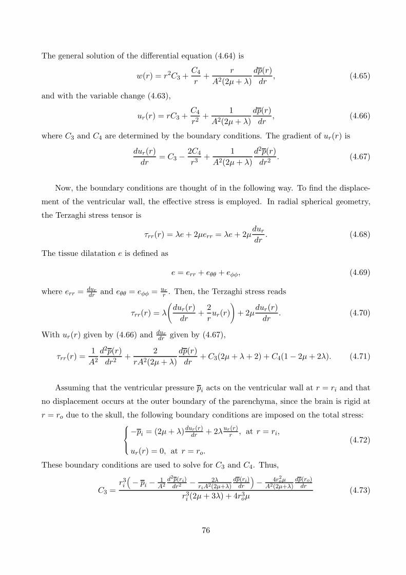
The general solution of the differential equation (4.64) is

w(r) = r2C3 +C4

r+

r

A2(2μ + λ)dp(r)dr

, (4.65)

and with the variable change (4.63),

ur(r) = rC3 +C4

r2+

1A2(2μ + λ)

dp(r)dr

, (4.66)

where C3 and C4 are determined by the boundary conditions. The gradient of ur(r) is

dur(r)dr

= C3 −2C4

r3+

1A2(2μ + λ)

d2p(r)dr2

. (4.67)

Now, the boundary conditions are thought of in the following way. To find the displace-

ment of the ventricular wall, the effective stress is employed. In radial spherical geometry,

the Terzaghi stress tensor is

τrr(r) = λe + 2μerr = λe + 2μdur

dr. (4.68)

The tissue dilatation e is defined as

e = err + eθθ + eφφ, (4.69)

where err = durdr and eθθ = eφφ = ur

r . Then, the Terzaghi stress reads

τrr(r) = λ

(dur(r)

dr+

2rur(r)

)+ 2μ

dur(r)dr

. (4.70)

With ur(r) given by (4.66) and durdr given by (4.67),

τrr(r) =1A2

d2p(r)dr2

+2

rA2(2μ + λ)dp(r)dr

+ C3(2μ + λ + 2) + C4(1 − 2μ + 2λ). (4.71)

Assuming that the ventricular pressure pi acts on the ventricular wall at r = ri and that

no displacement occurs at the outer boundary of the parenchyma, since the brain is rigid at

r = ro due to the skull, the following boundary conditions are imposed on the total stress:⎧⎪⎨⎪⎩−pi = (2μ + λ)dur(r)

dr + 2λur(r)r , at r = ri,

ur(r) = 0, at r = ro.

(4.72)

These boundary conditions are used to solve for C3 and C4. Thus,

C3 =r3i

(− pi − 1

A2d2p(ri)

dr2 − 2λriA2(2μ+λ)

dp(ri)dr

)− 4r2

oμA2(2μ+λ)

dp(ro)dr

r3i (2μ + 3λ) + 4r3

oμ(4.73)

76

and

C4 =r2i r

2o

[ro

(ripi + ri

A2d2p(ri)

dr2 + 2λA2(2μ+λ)

dp(ri)dr

)− ri(2μ+3λ)

A2(2μ+λ)dp(ro)

dr

]r3i (2μ + 3λ) + 4r3

oμ. (4.74)

where p(ri) and p(ro) are the boundary conditions (4.46), and

dp(ri)dr

=−roApv

ri sinh(A(ro − ri))− A(pi − pv) cosh(A(ro − ri))

sinh(A(ro − ri))+

pv − pi

ri, (4.75)

dp(ro)dr

=−Apv cosh(A(ro − ri))

sinh(A(ro − ri))+

pv

ro− A

ri

ro

(pi − pv)sinh(A(ro − ri))

, (4.76)

and

d2p(ri)dr2

= −(pi − pv)[

2r2i

+A cosh(A(ro − ri))ri sinh(A(ro − ri))

]

+ A(pi − pv)[

cosh(A(ro − ri))ri sinh(A(ro − ri))

+ A

]+

2roApv

r2i sinh(A(ro − ri))

. (4.77)

Substituting C3 from (4.73) and C4 from (4.74) into the general solution (4.66) results in the

formula for the radial displacement of the parenchyma tissue at steady state.

The steady state radial displacement solution is messy; it has been checked using MAT-

LAB that the solution satisfies the radial displacement differential equation and boundary

conditions. However, one can evaluate dp(r)dr (4.55) at ri and ro as well as d2p(r)

dr2 (4.56) at ri

and simplify the results by the approximation that sinh(x) → cosh(x) as x → ∞. Since the

value of A in the argument of sinh and cosh is large enough for this approximation to be

accurate to 9 decimal places, the derivates can be written as follows:

dp(ri)dr

= − roApv

ri sinh(A(ro − ri))− (pi − pv)(1 + riA) cosh(A(ro − ri))

ri sinh(A(ro − ri)); (4.78)

dp(ro)dr

=pv(1 − roA) cosh(A(ro − ri))

ro sinh(A(ro − ri))− A

ri

ro

(pi − pv)sinh(A(ro − ri))

; (4.79)

and

d2p(ri)dr2

=ri(pi − pv) cosh(A(ro − ri))

sinh(A(ro − ri))

[2r3i

+2A

r2i

+A2

ri

]+

2roApv

r2i sinh(A(ro − ri))

. (4.80)

Equations (4.78), (4.79), and (4.80) can be substituted in the expression for C3 given by

(4.73) and the expression for C4 given by (4.74); however, the radial displacement solution

(4.66) remains complex nevertheless.

77

4.3 Results

In this Section, the steady state results for both the pressure and the ventricle displace-

ment are given and compared with Levine’s (1999) results for the SEPA hypothesis.

4.3.1 Parameters

The radial values for the brain are chosen to represent a brain that has been altered due

to normal pressure hydrocephalus. The ventricle wall and the outer edge of the parenchyma

are at ri = 4 cm and ro = 8 cm, as found in Levine (1999) for the SEPA hypothesis. It

is assumed that parenchymal compression has occurred (due to the ventricular expansion),

since Levine (1999) states that in a normal brain without any ventricular expansion, ri = 2

cm.

All pressure values for the new model are relative to the atmospheric pressure of 760

mmHg. A characteristic feature of normal pressure hydrocephalus is that the ventricular

pressure (or the intracranial pressure) is identical to that of a normal brain. The normal

range for intracranial pressure is measured to be 0 − 10 mmHg. At the upper limit of the

normal range, 20 − 25 mmHg, treatment should be initiated to relieve the brain pressure

(Ghajar, 2000). Thus, in the mixture-theory based model, the ventricular pressure pi at ri

is taken to be 15 mmHg, as the average of the higher extreme of the normal range and the

lower extreme of the upper limit. At r = ro, the pressure is assigned to be the atmospheric

pressure of 0 mmHg, since the subarachnoid space is in contact with the sagittal sinus; the

sagittal sinus pressure is 3 − 8 mmHg relative to the atmospheric pressure, and may fall as

low as −10 mmHg (Albright et al., 1991); so 0 mmHg is roughly the average. The venous

pressure pv in the brain is varied so that its effects on the model can be investigated. The

values of pv which are used in the model are -5 mmHg, -2 mmHg, and 0 mmHg.

The parameter A2 is defined as Lp

KSV , where Lp is the permeability of the veins, S

V is the

surface area density of the veins, and K is the hydraulic conductivity of the parenchyma.

Assuming that the brain tissue is similar to normal tissue, the values for A2 are taken from

Jain et al., (2007), noting that the values quoted for the capillaries are used for the veins as a

crude approximation: Lp = 3.6× 10−8 cm second−1 mmHg−1, K = 2.5× 10−7 cm2 second−1

mmHg−1, and SV = 50 − 250 cm−1. From these, the dimension of A2 is easily calculated to

be L−2, where L represents length. The values for A21, A2

2, and A23 are calculated by varying

78

SV from the lower extreme of 50 cm−1, to the average of 150 cm−1, and to the higher extreme

of 250 cm−1, as seen in Table 4.1. Also, in Levine (1999), the parameter k = k′

k(where the

permeability coefficient k′ comes from Darcy’s law and the absorption coefficient k comes

from Starling’s law) has the units cm2, or the dimension of L2. One can write the inversely

proportional relation between A2 and k,

A2 =1k, (4.81)

and Table 4.1 shows the corresponding k values as well. For the value k4, Levine uses 0.1 cm2

in his analysis, and the corresponding A24 is 10 cm−2 by equation (4.81). Since the actual

values for k′ and k are not given when considering k4, the values for K and Lp are used to

calculate the values for SV . In other words, since k = k′

k= 0.1 cm2 for Levine, and in the

mixture-theory based model, k = 1A2 = K

LpSV

, the vascular surface density is extracted from

the equation 10 = KLp

SV

by using the values K and Lp from Jain et al., (2007).

Vascular surface area density SV (cm−1) A2

i (cm−2) ki (cm2)

50 A21 = 7.2 k1 = 0.14

150 A22 = 21.6 k2 = 0.05

250 A23 = 36 k3 = 0.03

69 A24 = 10 k4 = 0.1

Table 4.1: Parameter values for A2 and k

The values of the elastic moduli are needed for the displacement distribution. For the

mixture-theory based model, the Lame parameters are taken from Chapter 2; the values

μ = 3.6 × 104 mmHg and λ = 1.5 × 105 mmHg, to ensure consistency with the assumptions

made in mixture theory (that asymptotic values for the solid matrix are used, and not those

of the biological tissue). Also, the elastic moduli in Levine (1999) are taken for comparison

purposes. Levine mentions that the Poisson ratio ν is 0.35 and provides the following values

for Young’s modulus E: the range 1−2×104 Nm−2 and 1×103 Nm−2, as cited in Taylor and

Miller (2004). Converting the Young’s modulus values into millimeters of mercury and fixing

ν = 0.35, the corresponding Lame’s coefficients are calculated using the following relations:

μ =E

2(1 + ν), (4.82)

79

and

λ =Eν

(1 + ν)(1 − 2ν). (4.83)

Table 4.2 shows the Lame coefficients when Young’s modulus is varied with a fixed Poisson

ratio.

E (Nm−2) E (mmHg) μ (mmHg) λ (mmHg)

1 × 103 7.5 2.8 6.5

1 × 104 75 27.8 64.8

2 × 104 150 55.6 129.6

Table 4.2: Levine (1999) Lame coefficient values with fixed ν = 0.35

4.3.2 Radial steady state pressure distribution

The radial steady state pressure profiles were obtained from

p(r) =−ropv

r

sinh(A(r − ri))sinh(A(ro − ri))

+ri(pi − pv)

r

sinh(A(ro − r))sinh(A(ro − ri))

+ pv, (4.84)

using the A2 values from Table 4.1, and varying the venous pressure pv. The results are

shown in Figures 4.1-4.4.

From these figures, it is evident that the larger the value of A2 is – that is, the larger the

value of SV is – the faster the pressure drops from its value at r = ri to the venous pressure pv,

before increasing to the atmospheric pressure po close to r = ro. All figures show that CSF is

absorbed at locations between 4.5 cm and 5.5 cm in the parenchyma. Furthermore, the value

of pv plays a profound role in the behavior of the steady state pressure distribution. If pv is

slightly less than po, then the pressure from the ventricle wall drops to pv and rebounds back

to po close to the outer edge of the parenchyma. If pv is equal to 0 mmHg, then equation

(4.84) becomes

p(r) =ripi

r

sinh(A(ro − r))sinh(A(ro − ri))

, (4.85)

which coincides with Levine’s (1999) steady state solution (4.8). In this case, CSF absorption

occurs approximately within a centimeter from the ventricular wall and the pressure remains

constant throughout the parenchyma all the way to the outer edge. This means that most of

the CSF absorption occurs very close to the ventricular wall.

80

4 5 6 7 8−5

0

5

10

15

radius (cm)

pres

sure

(mm

Hg)

pv = −5 mmHg pv = −2 mmHg pv = 0 mmHg

A2

1 = 7.2 cm−2

Figure 4.1: Steady state pressure profile with A21 = 7.2 cm−2

Finally, it is important to mention the effect of pv below the atmospheric pressure. When

pv is less than 0 mmHg, the IFP slightly increases near the outer boundary. This implies that

the filtration velocity, given by Darcy’s law, reverses its direction and a small amount of CSF

from the subarachnoid space enters the brain parenchyma to be absorbed nearby. This effect

has been observed by Kenyon (1976a) who refers to it as ”retrograde filtration”. In Figures

4.1-4.4, the retrograde filtration is hardly noticeable when the venous pressure is very close

to atmospheric pressure.

81

4 5 6 7 8−5

0

5

10

15

radius (cm)

pres

sure

(mm

Hg)

pv = −5 mmHg pv = −2 mmHg pv = 0 mmHg

A2

2 = 21.6 cm−2

Figure 4.2: Steady state pressure profile with A22 = 21.6 cm−2

4 5 6 7 8−5

0

5

10

15

radius (cm)

pres

sure

(mm

Hg)

pv = −5 mmHg pv = −2 mmHg pv = 0 mmHg

A2

3 = 36 cm−2

Figure 4.3: Steady state pressure profile with A23 = 36 cm−2

82

4 5 6 7 8−5

0

5

10

15

radius (cm)

pres

sure

(mm

Hg)

pv = −5 mmHg pv = −2 mmHg pv = 0 mmHg

A24 = 10 cm−2

Figure 4.4: Steady state pressure profile with A24 = 10 cm−2

4.3.3 Radial steady state displacement distribution

According to the mixture theory model, the radial steady state displacement ur(r) is

given by equations (4.66) and (4.73)-(4.77). Its numeric values are presented in Table 4.3;

the first column shows the range of values of A2, as in Table 4.1, and the second column

indicates the range of values of the venous pressure. The value of the ventricular radius is

ri = 4 cm, as in Levine (1999), under the SEPA hypothesis, and the elastic parameters are

μ = 3.6 × 104 mmHg and λ = 1.5 × 105 mmHg as used before. Since in all cases the values

of ur(ri) are negligible, it clearly shows that the ventricular displacement is independent of

the vascular surface area density SV and of the venous pressure pv.

83

A2i (cm−2) pv (mmHg) ur(ri) (cm)

−5 5.6 × 10−4

A21 = 7.2 −2 5.2 × 10−4

0 4.9 × 10−4

−5 5.7 × 10−4

A22 = 21.6 −2 5.2 × 10−4

0 5.0 × 10−4

−5 5.7 × 10−4

A23 = 36 −2 5.3 × 10−4

0 5.0 × 10−4

−5 5.6 × 10−4

A24 = 10 −2 5.2 × 10−4

0 5.0 × 10−4

Table 4.3: Ventricular displacement ur(ri) according to the

mixture theory model

μ, λ (mmHg)

2.8, 6.5

55.6, 129.6

A2i (cm−2) pv (mmHg) ur(ri) (cm)

−5 8.1

A21 = 7.2 −2 7.6

0 7.2

−5 8.4

A23 = 36 −2 7.7

0 7.3

−5 0.41

A21 = 7.2 −2 0.38

0 0.36

−5 0.42

A23 = 36 −2 0.39

0 0.37

Table 4.4: Ventricular displacement ur(ri) according to the elastic

parameters suggested by Levine (1999) with ri = 4 cm

84

The ventricular displacement becomes extremely sensitive when changing the elastic pa-

rameters μ and λ (or G and ν in the notation by Levine (1999)). When μ = 2.8 mmHg and

λ = 6.5 mmHg, for any A2 and pv values, the ventricular displacement ranges from 7.2 cm

to 8.4 cm which is far too large. The brain parenchyma would be severely compressed. Also,

Levine’s model predicts compression of the brain beyond the outer boundary which is set at

8 cm which is clearly not realistic. These values are not an error in the calculations using

the mixture theory model. Furthermore, for the case when μ = 55.6 mmHg and λ = 129.6

mmHg, the ventricular wall displacement, for any A2 and pv values, ranges from 0.36 cm to

0.42 cm. Here, these displacement values seem acceptable to explain normal pressure hydro-

cephalus; however, the Lame parameters represent of the values of the brain tissue and not of

the asymptotic values of the solid matrix in accordance to the assumptions made in mixture

theory.

85

Chapter 5

Discussion and conclusion

The center of attention of this Thesis is the development of mathematical models, using

theory of poroelasticity (developed in the study of the flow through a porous medium), and

their application to biological tissues.

Two mechanisms suggest a time dependence when describing the flow through a porous

medium. The first mechanism occurs as the fluid permeates an elastic porous material. The

drag force between the fluid and the solid may cause the solid matrix to deform. Conversely,

the solid matrix can deform due to a force being applied to it, which may induce a fluid

flow in the pores. These mechanisms can be coupled, and the mechanical properties of the

material assume a time-dependent character.

The theory of poroelasticity has a long and distinguished history, which one can find in

a recent monograph by de Boer (2000). There exist two versions of the theory:

a. Consolidation Theory, developed by M. Biot (1941) in the context of soil mechanics and

ground waterflow; and

b. Mixture Theory, whose name derives from early theoretical developments involving mix-

tures of gases (de Boer, 2000).

The two versions have been shown to be equivalent (e.g. Simon, 1992); however, in this work,

the Mixture Theory version of poroelasticity is employed because of its sharper theoretical

formulation.

Chapter 2 uses Mixture Theory to derive a mathematical model that explains the mech-

anism responsible for the increase of the IFP in solid tumors. A similar model, also using

Mixture Theory, was previously formulated by Netti et al. (1995, 1997) from a different point

of view. The model starts with the IFP steady state in a fully developed tumor. Artificially,

the IFP is perturbed from its steady state in order to study the response of the IFP when

86

the vascular pressure was increased and later, decreased. One of the main findings was that

the changes in IFP are closely related to the vascular pressure variations with a time delay

of approximately 10 seconds. The time delay is highly influenced by the choice of the Lame

parameters – i.e., the stiffness parameters λ and μ – reputedly valid for soft biological tissue.

As mentioned in the analysis of Chapter 2, the Lame parameters for biological tissue

are inconsistent with one of the fundamental assumptions of Mixture Theory. The param-

eter should be that of only the solid matrix, and the viscoelasticity of the solid constituent

is negligible. In Appendix A where Mixture Theory is formulated, it is pointed out that the

asymptotic values of the elastic moduli λ and μ must be used. Although these values have

never been reported in literature, the order of magnitude of the elastic moduli should be

greater than those reported by Netti et al. (1995, 1997), close to the measured values for

saturated soft clay, listed in Table 2.2 and used in the simulations. The elastic moduli values

have a profound effect on the identification of the appropriate time scale over which the IFP

grows to reach the observed elevated value at steady state.

In fact, Netti et al. (1995, 1997) define the time scale by the parameter

T =R2

K(2μ + λ), (5.1)

which arises from the non-dimensionalization of the mathematical problem, whereas Chapter

2 identifies the time scale which is linked the type of a solid tumor. Based on Chapter 2,

equation (2.24),

Lp(t) = L0p

[1 + C

(1 − e−Dt

)], (5.2)

the IFP steady state is obtained as soon as the value of the vascular permeability Lp(t)

reaches very close to Lp(∞). In turn, the rate at which steady state is reached depends on

the parameter D that represents the rate of tumor growth, which is known to vary from tumor

to tumor (Bates and Curry, 1996). Some typical values of this parameter are shown in Table

2.3, and are used to simulate the steady state and the transient IFP profile, shown in Figure

2.5-2.7 for a fixed location inside the tumor. These figures clearly show that the pressure

trend is the same, but the time for when steady state is reached is different depending on the

tumor type.

The existence of different time scales has already been found experimentally by Khosra-

vani et al. (2004) and by Milosevic et al. (2008). With a sudden insertion of a needle into the

87

center of the tumor (which was part of the measurement system), the transient fluid response

was recorded. To understand the cause of the IFP behavior, simulations were created, based

on a discrete mathematical model which does not use poroelasticity theory. The conclusion

was that the shape and the time period of the pressure recordings were due to the variations of

the hydraulic conductivity K in the tumor interstitium. However, the Mixture Theory model

in Chapter 2 offers an alternative explanation of the existence of different time scales. It is

difficult to say more than this until in situ measurements of K can be done, which requires

overcoming serious technical challenges as stated in Milosevic et al. (2008).

A second investigation using Mixture Theory is reported in Chapter 3 of this Thesis, but

for the moment its discussion is postponed in order to proceed first with the application found

in Chapter 4. As stated in Chapter 1, the objective is to determine whether a Mixture Theory

based mathematical model can explain the pathogenesis of normal pressure hydrocephalus

under the hypothesis that most of the cerebrospinal fluid (CSF) is effectively absorbed in

the brain parenchyma, rather than in the arachnoid villi as commonly believed. The idea

is that as CSF crosses the ventricular wall and flows through the parenchymal interstitium

to be absorbed by the venous blood, it drags along the solid matrix and produces a finite

displacement of the ventricular wall. As the wall expands, the permeability of the wall

increases and smaller pressure gradients are needed to push the CSF into the parenchyma, so

that the intracranial pressure is indistinguishable from that of the pressure in a normal brain.

This hypothesis has been adopted by Levine (1999) and analyzed using Biot’s consolidation

theory along with the addition of Starling’s law – or a reduced form of it.

The mathematical model constructed and used in Chapter 4 shows that Levine’s con-

clusions are not tenable, because the displacements of the ventricular wall implied by the

parenchymal absorption hypothesis are negligible. Interestingly enough, a similar conclusion

was reached by Sobey and Wirth (2006), where consolidation theory was also used under

the assumption that the parenchymal permeability is a function of the dilatation. The use

of a Poiseuille-like law describes the fluid mechanics of the CSF flowing in the aqueduct of

Sylvius.

In the analysis of Levine (1999), several misunderstandings of consolidation theory appear

and need to be addressed. For instance, the nature of the porous medium being the brain is

defined as: ”The parenchyma consists of three components: a solid matrix permeated by two

networks of fluid-filled channels. [...] The first fluid network consists of the interstitial fluid

88

in the interconnected channels of extracellular space. [...] The second fluid network consists

of the blood in the cerebral vessels [...]. Although all of the solid and fluid elements are

intrinsically incompressible [...] the three components of the parenchyma are analogous to a

porous soil consisting of solid, incompressible elements (the solid matrix) and pores occupied

by both water (interstitial fluid) and pockets of air (intravascular blood)” (Levine, 1999,

pages 880-881). This is not a proper analogy. The gas phase in Biot’s consolidation theory

is compressible, while the intravascular blood is not, by the assumption in Levine (1999). In

fact, when describing the meaning of the parameters α and Q in the formula for the variation

of the pore water content θ,

θ = αε +σ

Q, (5.3)

where ε is the dilatation and σ is the pore pressure, Biot (1941) states that: ”It is quite

obvious that the constants α and Q will be of significance for a soil not completely saturated

with water and containing air bubbles” (Biot, 1941, page 159).

Another misunderstanding of the poroelasticity theory occurs when the values of elastic

moduli for the porous medium are discussed in Levine (1999). Very low values are favored for

the shear modulus G (approximately 400 Nm2 ) and the Poisson ratio ν (about 0.35). Moreover,

it is suggested that in later stages of normal pressure hydrocephalus both G and ν increase

because the brain becomes more rigid. This contradicts the initial assumption that all the

poroelasticity parameters are constant.

These problems do not occur in the derivation of the mathematical model based on

Mixture Theory in Chapter 4. As already mentioned in connection with the work done in

Chapter 2, the values of the elastic moduli must be chosen so that the viscoelasticity of the

solid matrix is negligible. Furthermore, there is no confusion about the pore water content θ

as in Biot (1941), for both the water content and the solid content are represented by their

respective volume fractions. This follows from the homogenization procedure, which starts

from the individual equations for the fluid and the solid and then is averaged to produce a

mixture in which each point contains both the fluid and the solid phases. Thus, the fluid and

solid volume fractions become scalar fields – see Appendix A for details.

The mathematical models presented in this Thesis are still limited by the assumptions

necessary in the formulation of Mixture Theory. Among the assumptions are:

i. Homogeneity and isotropy;

89

ii. Linearity of the stress-strain relations;

iii. Small strains; and,

iv. Validity of Darcy’s law and the modified version of Starling’s law (i.e., the complete

neglect of the osmotic pressure).

In Chapter 2, a further assumption is made to make the mathematical work more manageable,

which is common with most other works (e.g., Netti et al., 1995, 1997). The pore pressure

is taken to be proportional to the tissue dilatation. Chapter 3 investigates the validity of

this assumption by solving the exact system of PDEs and comparing the results with the

proportionality assumption. To simplify the calculations, the case of no sinks or sources is

considered in Chapter 3 for a hollow spherical sand drain. This is analogous with the work

done by De Leeuw (1965) for a hollow cylindrical sand drain. The conclusion is that the

proportionality, in general, is quite poor. As a result, a future direction of research would be

to extend the work in Chapter 3 by adding a source and/or sink terms to test against the

model used in Chapter 2.

90

Appendix A

Formulation of mixture theory

The main focus of this Appendix A is to present the formulation of mixture theory in

detail. The reader can also refer to Kenyon (1976b) for a more general and in depth derivation

of mixture theory.

In mixture theory, the continuum is modeled as a poroelastic medium in which the pores

are completely filled with a Newtonian viscous fluid and the solid skeleton is linearly elastic.

The medium is initially homogeneous and both phases are intrinsically incompressible; that

is, the unjacketed compressibility (Biot and Willis, 1957) is negligible for the range of pore

pressure intended here, and compression of the medium occurs only because of a redistribution

of the fluid and the solid components. Inertia forces associated with seepage in the matrix

are negligible because the Reynolds number based on pore size is much smaller than 1.

Furthermore, the inertia in the bulk material is disregarded as long as the relaxation time for

the constant strain is much shorter than the consolidation time. Finally, the effects due to

matrix viscoelasticity will be negligible provided that the relaxation time for solid dilatation

is small compared to the consolidation time and that the asymptotic values of the elastic

moduli μ and λ are used to characterize the matrix stiffness (Kenyon, 1976b). Roughly

speaking, this means that the rate of change of volume in the bulk material is assumed to be

limited by the speed with which fluid can enter the pores, and not by the speed with which

the matrix can relax independently of pore fluid flow.

The domain of the homogeneous continuum is taken to be a subset D ⊂ IR3. Spatial

and temporal coordinates are denoted by r and t respectively. Define F (r, t) to be the

difference between the source of fluid and the sink of fluid per unit time while the solid phase

91

is conserved. On D, the conservation of mass equation for the fluid phase f and the solid

phase s in the presence of F (r, t) is written as:

∂ρf

∂t+ ∇ ·

(ρfvf

)= F (A1)

∂ρs

∂t+ ∇ · (ρsvs) = 0, (A2)

where ρf and ρs are the apparent densities and vf and vs are the velocities. Adding term by

term equations (A1) and (A2), it yields

∂ρ

∂t+ ∇ · (ρv) = F, (A3)

where the mass density is ρ = ρf + ρs and the momentum density is ρv = ρfvf + ρsvs.

The first step is to rewrite equations (A1) and (A2) in terms of true density ρT defined

as:

true mass density of fluid: ρfT = ΔM f/ΔV f

true mass density of solid: ρsT = ΔM s/ΔV s.

In what follows, ρfT and ρs

T are assumed dependent on t only (and not on the location in

space). The relation between apparent density and true density of the fluid phase is

ρf =ΔM f

ΔV=

ΔM f

ΔV f

ΔV f

ΔV= ρf

Tφf (A4)

where φf = ΔV f/ΔV is the volume fraction of the fluid. Likewise,

ρs =ΔM s

ΔV=

ΔM s

ΔV s

ΔV s

ΔV= ρs

Tφs (A5)

where φs = ΔV s/ΔV is the volume fraction of the solid. Note that φf and φs are functions

of both r and t and are related by φf + φs = 1 which means that the biphasic material is

completely saturated. Thus, using equations (A4) and (A5) in (A1) and (A2) gives

∂ρfTφf

∂t+ ∇ ·

(ρf

Tφfvf)

= F (A6)

∂ρsTφs

∂t+ ∇ · (ρs

Tφsvs) = 0. (A7)

Next, taking into account the assumption that each phase is incompressible and expanding

equations (A6) and (A7), it follows that

∂φf

∂t+ ∇ ·

(φfvf

)= q(r, t) (A8)

92

∂φs

∂t+ ∇ · (φsvs) = 0, (A9)

where the quantity on the right hand side of equation (A8) is q(r, t) = F

ρfT

.

Adding term by term equations (A8) and (A9), and taking into account the condition of

full saturation, φf + φs = 1, gives

∇ ·(φfvf + (1 − φf )

∂u

∂t

)= q, (A10)

where u is the solid displacement vector. From equation (A10), the volumetric flux M can

be extracted:

M =(φfvf + (1 − φf )

∂u

∂t

)= N +

∂u

∂t, (A11)

where N is the relative velocity of the fluid and the solid:

N = φf

(vf − ∂u

∂t

). (A12)

Then, by Darcy’s law, it follows that

N = −k

η∇p = −K∇p, (A13)

where k is the permeability of the porous medium, η is the shear viscosity of the fluid and p

is the pore fluid pressure. The constant K equals k divided by η. Since ∇ · M = q(r, t), the

refined result is

∂e

∂t− K∇2p = q, (A14)

where e = ∇ · u is the solid or tissue dilatation.

Now, conservation of momentum equations for each phase are introduced as:

ρf

(∂vf

∂t+ vf · ∇vf

)= ∇ · T

f (A15)

ρs

(∂vs

∂t+ vs · ∇vs

)= ∇ · T

s, (A16)

where Tf and T

s are the stress tensors for the fluid and the solid respectively. Body forces

are neglected in equations (A15) and (A16) due to the very small effect on the continuum.

Inertia forces associated with seepage in the matrix are negligible on the grounds that the

Reynolds number based on pore size is much smaller than one and that the relaxation time

93

for constant strain of the bulk material is much shorter than the consolidation time. Thus,

neglecting body forces and inertia forces reduces the above equations to:

∇ · Tf = 0 (A17)

∇ · Ts = 0. (A18)

Now, the form of the constitutive equation for the fluid phase is

Tf =

(−φfp + ξ∇ · vf

)I + 2ηD, (A19)

where p is the pore fluid pressure, ξ is the second viscosity coefficient, I is the identity matrix,

η is the shear viscosity, and D is the rate of strain. Note that the fluid phase is incompressible

which implies that ∇ · vf = 0, then equation (A19) becomes

Tf = −φfpI + 2ηD, (A20)

which is approximately

Tf ≈ −φfpI. (A21)

Equation (A20) holds under the assumption of mixture theory that the fluid phase is a

Newtonian viscous fluid. Hence, equation (A21) implies that the tensor D is negligible on the

grounds that the contact forces of the solid phase are greater than the viscous forces of the

fluid phase. Finally, the constitutive equation for the solid phase is written as:

Ts = (−φsp + λs∇ · u) I + 2μsε, (A22)

where λs and μs are Lame’s elasticity parameters and ε is the strain tensor.

The relation of these tensors to the other field variables – i.e., the constitutive theory

of a general incompressible fluid-solid mixture – has been given by Kenyon (1976b) among

others. Specialized to this system, using equations (A21) and (A22), a constitutive equation

for the whole mixture is derived. This is done by adding equations (A21) and (A22) and by

employing the fact that the biphasic material is completely saturated, φs + φf = 1:

Tm = T

f + Ts = −pI + τij , (A23)

where m represents the mixture and τij is the contact stress defined as

τij = λeI + 2με. (A24)

In order to avoid clutter, the elasticity parameters will be denoted as μ and λ.

94

In the derivation of mixture theory, Kenyon (1976b) pointed out that the pore fluid

pressure p produces an effective bulk area-averaged hydrostatic pressure in the fluid in the

mixture of amount φfp. Similarly, it produces an effective bulk area-averaged hydrostatic

pressure of amount φsp in the solid. It has no other effect on the solid, in the sense that

the pore pressure acting on the solid elements does not produce any change in shape and,

in particular, does not induce any ‘cell–to–cell’ contact. Therefore, the contact stress τij of

equation (A24) coincides with the Terzaghi stress (Terzaghi, 1943).

Then, the equation of motion becomes

∇ · Tm = ∇ ·

(T

f + Ts)

= 0, (A25)

which reduces to

−∇p + (μ + λ)∇(∇ · u) + μ∇2u = 0. (A26)

Taking the divergence of each term and remembering the fact that e = ∇ · u is the solid

dilatation, equation (A26) can be written as

(2μ + λ)∇2e = ∇2p. (A27)

Together with e = ∇·u, equations (A14) and (A26) form a closed system of five equations

with five unknown variables: e, p, and the three components of u.

95

Appendix B

Relation between tissue dilatation and interstitial fluidpressure

In this Appendix, the relation between the tissue dilatation e and the interstitial fluid

pressure (IFP) p is discussed in detail. As shown in Appendix A, the form of this relation

depends crucially on the harmonic function f given by equation (A30). In particular, when

f = 0, then e and p are proportional, and this assumption was used by Netti et al. (1995,

1997) as well as in follow-up works - including this one, in particular in Chapter 2. It is,

therefore, clearly of interest to ascertain whether this assumption can be justified on physical

and/or mathematical grounds.

It should be noted that this problem is not new, for it was first investigated by researchers

studying the dynamics of fluids in porous media (Verruijt, 1969; Bear, 1988), particularly in

the study of unsteady ground water flow in compressible soils. The appeal of the assumption

f = 0 is due to the fact that the entire three-dimensional system of partial differential equa-

tions embodying consolidation theory (Biot, 1941), as well as mixture theory, is reduced to a

single parabolic equation for the pore pressure. But despite many attempts, the hypothesis

f = 0 could be justified only for a single case, namely that of cylindrical body satisfying the

conditions of plane strain and axial symmetry, as shown by De Leeuw (1965).

First, the general relation between e and p, namely

p − (2μ + λ)e = f, (B1)

is employed to eliminate the gradient of e and p from the equation of motion, as follows.

Assuming that u is radial symmetric, i.e., u = u(r)er, where er is the unit vector of the r

component, and using spherical coordinates, equation (B1) is shown to imply

(2μ + λ)∂e

∂r+

∂f

∂r=

∂p

∂r. (B2)

96

Now, under the same assumption, the equation of motion (same as equation (A27) in Ap-

pendix A) becomes

μ

(2r

∂ur

∂r+

∂2ur

∂r2− 2ur

r2

)+ (μ + λ)

∂e

∂r=

∂p

∂r. (B3)

The relation e = ∇ · u can be written as

e =2ur

r+

∂ur

∂r, (B4)

and so

∂e

∂r=

2r

∂ur

∂r+

∂2ur

∂r2− 2ur

r2. (B5)

This allows for the pressure gradient to be represented as

∂p

∂r= (2μ + λ)

(2r

∂ur

∂r+

∂2ur

∂r2− 2ur

r2

)+

∂f

∂r. (B6)

Substituting equations (B5) and (B6) into (B3) yields

∂f

∂r= μ

(2r

∂ur

∂r+

∂2ur

∂r2− 2ur

r2

)− μ

(−2ur

r2+

2r

∂ur

∂r+

∂2ur

∂r2

)= 0 (B7)

Thus, under radial symmetry assumed above, the harmonic function f depends only on time.

Furthermore, the assumption that all field quantities depend on r and t forces the solutions

of ∇2f = 0 to be in the form

f(r, t) =a(t)r

+ b(t), (B8)

where a(t) and b(t) are arbitrary functions of time. However, since ∂f∂r = 0, as shown in

equation (B7), it follows that

∂f

∂r= −a(t)

r2= 0. (B9)

This implies that a(t) = 0 which results in

f = b(t), (B10)

i.e., f being an arbitrary function of time.

97

Appendix C

Calculation of the analytic solution for the approxi-mated case in Chapter 3

Referring to Chapter 3, Section 3.2, the Laplace inverse of solution (3.44), namely

P (r, s) =riα sinh(

√sγ (ro − r)) + roβ sinh(

√sγ (r − ri))

rs sinh(√

sγ (ro − ri))

, (C1)

can be computed analytically. The techinque used here is adopted from Powers (1999), pages

379-381, since rarely does the inverse Laplace of transcendental functions appears in a table

of transforms. It is based on the following result:

Theorem

Let p and q be polynomials, q of lower degree than p, and let p have only simple

roots, r1, r2, ..., rk. Then

L−1

(q(s)p(s)

)=

q(r1)p′(r1)

er1t +q(r2)p′(r2)

er2t + ... +q(rk)p′(rk)

erkt. (C2)

By extending the above theorem to transcendental functions, the inverse transform of Equa-

tion (C1) is computed in the following way.

Part A

When r0 = 0, multiply equation (C1) by s − r0 = s to find A0 and take the limit as s

approaches r0. The right hand side goes to A0. On the left hand side,

A0(r) = lims→0

riα sinh(√

sγ (ro − r)) + roβ sinh(

√sγ (r − ri))

r sinh(√

sγ (ro − ri))

= lims→0

ri(ro − r)α cosh(√

sγ (ro − r)) + ro(r − ri)β cosh(

√sγ (r − ri))

r(ro − ri) cosh(√

sγ (ro − ri))

=ri(ro − r)α + ro(r − ri)β

r(ro − ri). (C3)

98

Thus, the portion of p(r, t) corresponding to s = 0 is

ri(ro − r)α + ro(r − ri)βr(ro − ri)

, (C4)

which is easily recognizable as the steady state solution.

Part B

When rn = −n2π2γ(ro−ri)2

for n = 1, 2, 3, ..., the term An(r) needs to be represented as

An(r) =q(rn)u′(rn)

. (C5)

From equation (C1), the numerator is q = riα sinh(√

sγ (ro − r)) + roβ sinh(

√sγ (r − ri)), and

the denominator is u = rs sinh(√

sγ (ro − ri)). Take

√rn = inπ

√γ

(ro−ri)in all the calculations.

Then,

An(r) =q(rn)u′(rn)

=riα sinh(ro−r√

γinπ

√γ

(ro−ri)) + roβ sinh(r−ri√

γinπ

√γ

(ro−ri))

r[sinh(ro−ri√

γinπ

√γ

(ro−ri)) + cosh(ro−ri√

γinπ

√γ

(ro−ri))]

=riα sinh( ro−r

ro−riinπ) + roβ sinh( r−ri

ro−riinπ)

r[sinh(inπ) + inπ

2 cosh(inπ)] . (C6)

Using the identities sinh(ix) = i sin(x) and cosh(ix) = cos(x), equation (C6) becomes

An(r) =riαi sin( ro−r

ro−rinπ) + roβi sin( r−ri

ro−rinπ)

r[inπ2 cos(nπ)

]=

2(−1)n

rnπ

[riα sin

(ro − r

ro − rinπ

)+ roβ sin

(r − ri

ro − rinπ

)]. (C7)

Hence, the portion of p(r, t) that arises from each rn is

An(r)exp(rnt) =2(−1)n

rnπ

[riα sin

(ro − r

ro − rinπ

)+ roβ sin

(r − ri

ro − rinπ

)]exp

(−(nπ)2γ(ro − ri)2

t

).

(C8)

Assembling the piece from Part A and Part B gives the full solution

p(r, t) = αri

r

[ro − r

ro − ri+

∞∑n=1

2(−1)n

nπsin

(ro − r

ro − rinπ

)exp

(−(nπ)2γ(ro − ri)2

t

)]

+ βro

r

[r − ri

ro − ri+

∞∑n=1

2(−1)n

nπsin

(r − ri

ro − rinπ

)exp

(−(nπ)2γ(ro − ri)2

t

)]. (C9)

99

Appendix D

Calculations of constants for the general solution inChapter 3

In this Appendix, the details of the calculation of the constants needed in Chapter 3,

Section 3.3 are given. Using the boundary conditions (3.83) and (3.85),⎧⎪⎪⎪⎪⎪⎪⎪⎪⎪⎪⎨⎪⎪⎪⎪⎪⎪⎪⎪⎪⎪⎩

P (qi, s) = αs ,

P (qo, s) = βs ,

τrr(qi, s) = 0,

τrr(qo, s) = 0.

(D1)

together with equations (3.63) and (3.81)

P (q, s) = (2μ + λ)√

π

2q

[A(s)I 1

2(q) + B(s)I− 1

2(q)

]+ G(s), (D2)

and

τrr(q, s) = λ

√π

2q

[A(s)I 1

2(q) + B(s)I− 1

2(q)

]

+ 2μ

√π

2q

[A(s)

(I 1

2(q) − 2

qI 3

2(q)

)+ B(s)

(I− 5

2(q) +

1qI− 3

2(q)

)]− 4

√s

γ

C(s)q3

,

(D3)

one obtains four equations for the four unknown constants – A(s), B(s), G(s), and C(s):

α

s= (2μ + λ)

√π

2qiI 1

2(qi)︸ ︷︷ ︸

Γi

A(s) + (2μ + λ)√

π

2qiI− 1

2(qi)︸ ︷︷ ︸

Φi

B(s) + G(s); (D4)

β

s= (2μ + λ)

√π

2qoI 1

2(qo)︸ ︷︷ ︸

Γo

A(s) + (2μ + λ)√

π

2qoI− 1

2(qo)︸ ︷︷ ︸

Φo

B(s) + G(s); (D5)

100

0 =[(2μ + λ)I 1

2(qi) −

4μ

qiI 3

2(qi)

]︸ ︷︷ ︸

Ωi

A(s)

+[λI− 1

2(qi) + 2μI− 5

2(qi) +

2μ

qiI− 3

2(qi)

]︸ ︷︷ ︸

Λi

B(s) − 4√

s1√

γ

1qi

3

√2qi

π︸ ︷︷ ︸Mi

√s

C(s); (D6)

0 =[(2μ + λ)I 1

2(qo) −

4μ

qoI 3

2(qo)

]︸ ︷︷ ︸

Ωo

A(s)

+[λI− 1

2(qo) + 2μI− 5

2(qo) +

2μ

qoI− 3

2(qo)

]︸ ︷︷ ︸

Λo

B(s) − 4√

s1√

γ

1qo

3

√2qo

π︸ ︷︷ ︸Mo

√s

C(s). (D7)

For simplicity, equations (D4)-(D7) are written as:

α

s= ΓiA(s) + ΦiB(s) + G(s); (D8)

β

s= ΓoA(s) + ΦoB(s) + G(s); (D9)

0 = ΩiA(s) + ΛiB(s) − Mi√

sC(s); (D10)

0 = ΩoA(s) + ΛoB(s) − Mo√

sC(s). (D11)

Equations (D10) and (D11) can be rewritten as:

0 =Ωi

MiA(s) +

Λi

MiB(s) −

√sC(s); (D12)

0 =Ωo

MoA(s) +

Λo

MoB(s) −

√sC(s). (D13)

Now, equation (D8) is subtracted from (D9), and equation (D14) is subtracted from (D13)

which yields:

(Γo − Γi)A(s) + (Φo − Φi)B(s) =β − α

s, (D14)

and ( Ωo

Mo− Ωi

Mi

)A(s) +

( Λo

Mo− Λi

Mi

)B(s) = 0, (D15)

101

respectively. The determinant of the linear system of equations (D14) and (D15) is

Δ = (Γo − Γi)( Λo

Mo− Λi

Mi

)− (Φo − Φi)

( Ωo

Mo− Ωi

Mi

). (D16)

Solving for A(s) and B(s) yields

A(s) =

(β−α

s

) (ΛoMo

− ΛiMi

)Δ

=(β − α)(ΛoMi − ΛiMo)

s(MiMo)Δ=

A(s)s

(D17)

and

B(s) =−

(β−α

s

) (ΩoMo

− ΩiMi

)Δ

=(α − β)(ΩoMi − ΩiMo)

s(MiMo)Δ=

B(s)s

, (D18)

respectively. Finally, the constant G(s) is given by either

G(s) =α

s− ΓiA(s) − ΦiB(s), (D19)

or

G(s) =β

s− ΓoA(s) − ΦoB(s). (D20)

(The constant C(s) is not needed.) The expansion of equations (D17), (D18) and (D19)

yields

A(s) =A(s)

s=

(β − α)(ΛoMi − ΛiMo)s[(Γo − Γi)(ΛoMi − ΛiMo) − (Φo − Φi)(ΩoMi − ΩiMo)]

, (D21)

B(s) =B(s)

s=

(α − β)(ΩoMi − ΩiMo)s[(Γo − Γi)(ΛoMi − ΛiMo) − (Φo − Φi)(ΩoMi − ΩiMo)]

, (D22)

and

G(s) =G(s)

s=

α

s− Γi

((β − α)(ΛoMi − ΛiMo)

s[(Γo − Γi)(ΛoMi − ΛiMo) − (Φo − Φi)(ΩoMi − ΩiMo)]

)

− Φi

((α − β)(ΩoMi − ΩiMo)

s[(Γo − Γi)(ΛoMi − ΛiMo) − (Φo − Φi)(ΩoMi − ΩiMo)]

). (D23)

Finally, plugging in equations (D21), (D22) and (D23) into equation (D2) gives the solution

for the test case:

P (q, s) = (2μ + λ)√

π

2q

[A(s)

sI 1

2(q) +

B(s)s

I− 12(q)

]+

G(s)s

. (D24)

The constants are rather complicated. However, writing each modified Bessel function

in terms of hyperbolic functions, or starting from scratch where solving the problem is done

solely using hyperbolic functions, allows the constants to be slightly simplified. First, the

102

determinant of the system of equations (D4)-(D7), modified by the substitution qi =√

Ari

and qo =√

Aro, where A = sγ , becomes:

Δ∗ =2μ + λ

A32

[(2μ + λ)A sinh(

√A(ro − ri))

(r2i

ro− r2

o

ri

)

+ 4μ sinh(√

A(ro − ri))( 1

ro− 1

ri

)

+4μA12 cosh(

√A(ro − ri))

(ri

ro+

ro

ri

)− 8A

12 μ

]. (D25)

Then, with A(s), B(s) and G(s) written using hyperbolic functions,

A(s)∗ =β − α

sA32 Δ∗

[(2μ + λ)A(r2

i cosh(√

Ari) − r2o sinh(

√Aro))

+4μ(cosh(√

Ari) − cosh(√

Aro)) − 4μ√

A(ri sinh(√

Ari) − ro sinh(√

Aro)];

(D26)

B(s)∗ =α − β

sA32 Δ∗

[(2μ + λ)A(r2

i sinh(√

Ari) − r2o sinh(

√Aro))

+4μ(sinh(√

Ari) − sinh(√

Aro)) − 4μ√

A(ri cosh(√

Ari) − ro cosh(√

Aro)];

(D27)

and, the constant G(s)∗ has two possible forms, one of which is

G(s)∗ =α

s+

(2μ + λ)(α − β)

sriA32 Δ∗

[(2μ + λ)Ar2

o sinh(√

A(ro − ri))

+4μ sinh(√

A(ro − ri)) + 4μ√

A(ri − ro cosh(√

A(ro − ri))]

(D28)

Now, substituting (D26), (D27) and (D28) into the equation (3.63) in Chapter 3, Section 3.3,

with q =√

Ar, yields

P (r, s) = (2μ + λ)[A(s)∗r√

Asinh(

√Ar) +

B(s)∗r

cosh(√

Ar)]

+ G(s)∗ . (D29)

Simplifying further, the Laplace-transformed expression for the test case in terms of hyper-

bolic functions is

P (r, s) =(2μ + λ)(α − β)

sA32 Δ∗

[1r

{(2μ + λ)A

[r2i sinh(

√A(ri − r)) − r2

o sinh(√

A(ro − r))]

+ 4μ[sinh(

√A(ri − r)) − sinh(

√A(ro − r))

]−4μ

√A

[ri cosh(

√A(ri − r)) − ro cosh(

√A(ro − r))

]}+

1ri

{(2μ + λ)Ar2

o sinh(√

A(ro − ri))

+4μ sinh(√

A(ro − ri)) + 4μ√

A(ri − ro cosh(√

A(ro − ri))}]

+α

s. (D30)

103

Equation (D30) is still messy; however, it is more manageable than the one that uses Bessel

functions.

104

References

M. Abramowitz and I. A. Stegun. Handbook of Mathematical Functions With Formulas,

Graphs, and Mathematical Tables. National Bureau of Standards Applied Mathematics

Series, Washington, 1964.

A. L. Albright, I. F. Pollack, and P. D. Adelson. Principles and practice of pediatric neuro-

surgery. Thieme New York, New York, 1999.

G. H. Algire and H. W. Chalkley. Vascular reactions of normal and malignant tissues in

vivo. I. Vascular reactions of mice to wounds and to normal and neoplastic transplants.

J. Nati. Cancer Inst., 6:73-85, Aug 1945.

D. O. Bates and F. E. Curry. Vascular endothelial growth factor increases hydraulic conduc-

tivity of isolated perfused microvessels. Am. J. Physiol. Society (Heart Circ. Physiol.),

271:H2520-H2528, Dec 1996.

L. T. Baxter and R. K. Jain. Transport of fluid and macromolecules in tumors I. Role of

interstitial pressure and convection. Microvasc. Res., 37:77-104, Jan 1989.

J. Bear, Dynamics of Fluids in Porous Media. American Elsevier Publishing Company, Inc.,

New York, 1988.

J. Bear and A. Verruijt, Modeling groundwater flow and pollution. D. Reidel Publishing

Company, New York, 1987.

M. A. Biot. General theory of three-dimensional consolidation. J. Appl. Phys., 12:155-164,

Feb 1941.

105

M. A. Biot and D. G. Willis. The Elastic Coefficients of the Theory of Consolidation. J.

Appl. Mech., 24:594-598, Dec 1957.

Y. C. Boucher, L. T. Baxter, and R. K. Jain. Interstitial Pressure Gradients in Tissue-Isolated

and Subcutaneous Tumors: Implications for Therapy. Cancer Res., 50:4478-4484, Aug

1990.

J. E. Bowles. Foundation analysis and design, fourth edition. McGraw-Hill Book Company,

New York, 1988.

P. Carmeliet and R. K. Jain. Molecular mechanisms and clinical applications of angiogenesis.

Nature, 473:298-307, Sep 2011.

Y. S. Chang, L. L. Munn, M. V. Hillsley, R. O. Dull, J. Yuan, S. Lakshminarayanan, T. W.

Gardner, R. K. Jain, and J. M. Tarbell. Effect of vascular endothelial growth factor on

cultured endothelial cell monolayer transport properties. Microvasc Res, 59:26577, Mar

2000.

B. D. Curti, W. J. Urba, W. G. Alvord, J. E. Janik, J. W. Smith II, K. Madara, and D.

L. Longo. Interstitial pressure of subcutaneous nodules in melanoma and lymphoma

patients: changes during treatment. Cancer Res, 53:2204-2207, May 1993.

R. de Boer. Theory of Porous Media. Highlights in the Historical Development and Current

Status. Springer, New York, 2000.

E. H. De Leeuw. The Theory of Three-dimensional Consolidation Applied to Cylindrical

Bodies. Proceedings of the 6th Int. Conf. of Soil Mechanics and Foundation Eng., 1:287-

290, 1965.

Y. C. Fung. Biomechanics. Springer-Verlag, New York, 1990.

J. Ghajar. Traumatic brain injury. The Lancet, 356:923-929, Sep 2000.

106

S. Goel, D. G. Duda, L. Xu, L. L. Munn, Y. Boucher, D. Fukumura, and R. K. Jain. Nor-

malization of the vasculature for treatment of cancer and other disease. Physiol. Rev.,

91:1071-1121, Jul 2011.

P. M. Gullino. Angiogenesis and oneogenesis. J Nat Cancer Inst, 61:639-643, 1976.

P. M. Gullino, S. H. Clark, and F. H. Grantham. The interstitial fluid of solid tumors. Cancer

Res, 24:780-797, Jun 1964.

R. Gutmann, M. Leunig, J. Feyh, A. E. Goetz, K. Messmer, E. Kastenbauer, and R. K. Jain.

Interstitial hypertension in head and neck tumors in patients: correlation with tumor

size. Cancer Res., 52:1993-1995, Apr 1992.

C. H. Heldin, K. Rubin, K. Pietras, and A. Ostman. High interstitial fluid pressure – an

obstacle in cancer therapy. Nature Rev., Cancer, 4:806-813, Oct 2004.

R. K. Jain. Transport of molecules in the tumor interstitium: A review. Cancer Res.,

47:3039-3051, Jun 1987a.

R. K. Jain. Transport of molecules across tumor vasculature. Cancer Metastasis Rev., 6:559-

594, Dec 1987b.

R. K. Jain. Normalizing tumor vasculature with anti-angiogenic therapy: a new paradigm

for combination therapy. Nat. Med., 7:987-989, Sep 2001.

R. K. Jain. Molecular regulation of vessel maturation. Nat. Med., 9:685-693, 2003.

R. K. Jain. Normalization of tumor vasculature: an emerging concept in antiangiogenic

therapy. Science., 307:58-62, 2005.

R. K. Jain. Taming vessels to treat cancer. Scientific American., 298:56-63, Jan 2008.

R. K. Jain and L. T. Baxter. Mechanisms of heterogeneous distribution of monoclonal anti-

bodies and other macromolecules in tumors: Significance of elevated interstitial pressure.

Cancer Res., 48:7022-7032, Dec 1988.

107

R. K. Jain, R. T. Tong, and L. L. Munn. Effect of Vascular Normalization by Antiangiogenic

Therapy on Interstitial Hypertension, Peritumor Edema, and Lymphatic Metastasis: In-

sights from a Mathematical Model. Cancer Res., 67:2729-2715, Mar 2007.

D. E. Kenyon. Transient filtration in a porous elastic cylinder. ASME J. Appl. Mech.,

43:594-598, Dec 1976a.

D. E. Kenyon. The theory of an incompressible solid-fluid mixture. Arch. Rat. Mech. Anal.,

62:131-147, Jun 1976b.

H. Khosravani, B. Chugh, M. F. Milosevic, and K. H. Norwich. Time response of interstitial

fluid pressure measurements in cervix cancer. Microvascular Res., 68:63-70, Jul 2004.

J. R. Less, M. C. Posner, Y. Boucher, D. Borochovitz, N. Wolmark, and R. K. Jain. Inter-

stitial hypertension in human breast and colorectal tumors. Cancer Res, 52:6371-6374,

Nov 1992.

D. N. Levine. The pathogenesis of normal pressure hydrocephalus: A theoretical analysis.

Bull. Math. Biol., 61:875-916, Sep 1999.

S. J. Lunt, A. Fyles, R. P. Hill, and M. Milosevic. Interstitial fluid pressure in tumors:

therapeutic barrier and biomarker of angiogenesis. (Report). Future Oncology, 10:793-

805, Dec 2008.

M. Milosevic, S. J. Lunt, E. Leung, J. Skliarenko, P. Show, A. Fyles, and R. P. Hill. Interstitial

permeability and elasticity in human cervix cancer. Microvascular Res, 75:381-390, Nov

2008.

S. D. Nathanson and L. Nelson. Interstitial fluid pressure in breast cancer, benign breast

conditions, and breast parenchyma. Ann Surg Oncol., 1:333-338, 1994.

P. A. Netti, L. T. Baxter, Y. Boucher, R. Skalak, and R. K. Jain. Time-dependent behavior

of interstitial fluid pressure in solid tumors: implications for drug deliver. Cancer Res.

55:5451-5458, Nov 1995.

108

P. A. Netti, L. T. Baxter, Y. Boucher, R. Skalak, and R. K. Jain. Macro- and Microscopic

Fluid Transport in Living Tissues: Application to Solid Tumors. AIChE Journal, 43:818-

834, Mar 1997.

J. Nolte. The human brain: An introduction to its functional anatomy. The C. V. Mosby

Company, Toronto, 1981.

T. M. Pocock, R. R. Foster, and D. O. Bates. Evidence of a role for TRPC channels in VEGF-

mediated increased vascular permeability in vivo. Am J Physiol Heart Circ Physiol,

286:H1015H1026, Oct 2003.

D. L. Powers. Boundary value problems, fourth edition. Harcourt/Academic Press, New

York, 1999.

P. H. Schurr and C. E. Polkey. Hydrocephalus. Oxford University Press, New York, 1993.

B. R. Simon. Multiphase poroelastic finite element models for soft tissue structures. Appl.

Mech. Rev., 45:191-217, 1992.

A. Smillie, I. Sobey, and Z. Molnar. A hydroelastic model of hydrocephalus. J. Fluid Mech.,

539:417-443, Apr 2005.

I. Sobey and B. Wirth. Effect of non-linear permeability in a spherically symmetric model of

hydrocephalus. Mathematical Medicine and Biology, 23:339361, 2006.

Z. Taylor and Z. Miller. Reassessment of Brain Elasticity for Analysis of Biomechanisms of

Hydrocephalus. Journal of Biomechanics, 37:1263-1269, Aug 2004.

G. Tenti, J. M. Drake, and S. Sivaloganathan. Brain biomechanics: mathematical modeling

of hydrocephalus. Neurol. Res., 22:19-24, Jan 2000.

Terzaghi, K. Theoretical Soil Mechanics. John Wiley and Sons, New York, 1943.

R. T. Tong, Y. Boucher, S. V. Kozin, F. Winkler, D. J. Hicklin, and R. K. Jain. Vascular

Normalization by Vascular Endothelial Growth Factor Receptor 2 Blockade Induces a

109

Pressure Gradient Across the Vasculature and Improves Drug Penetration in Tumors.

Cancer Res., 64:3731-3736, Jun 2004.

A. Verruijt. Flow Through Porous Media (R.J.M. De Wiest, ed.). Academic Press, New

York, 1969.

A. Verruijt. Theory of groundwater flow. Gordon and Breach Science Publishers Inc., New

York, 1970.

D. V. Widder. Advanced Calculus, Second Edition. Dover Publications, Inc., Mineola, 1989.

J. S. Young, C. E. Lumsden, and A. L. Stalker. The significance of the ”tissue pressure”

of normal testicular and of neoplastic (Brown-Pearce carcinoma) tissue in the rabbit. J.

Pathol. Bacteriol., 62:313-333, Jul 1950.

110