Building Block of a Programmable NeuromorphicSubstrate: A Digital Neurosynaptic Core

John V. Arthur∗‡, Paul A. Merolla∗, Filipp Akopyan∗, Rodrigo Alvarez∗,Andrew Cassidy∗, Shyamal Chandra∗, Steve Esser∗, Nabil Imam†,

William Risk∗, Daniel Rubin∗, Rajit Manohar†, and Dharmendra Modha∗∗IBM Almaden Research Center, Almaden, CA, USA

†Cornell University, Ithaca, NY, USA‡Email: arthurjo@us.ibm.com

Abstract—The grand challenge of neuromorphic computationis to develop a flexible brain-like architecture capable of awide array of real-time applications, while striving towards theultra-low power consumption and compact size of biologicalneural systems. To this end, we fabricated a key building blockof a modular neuromorphic architecture, a neurosynaptic core.Our implementation consists of 256 integrate-and-fire neuronsand a 1,024×256 SRAM crossbar memory for synapses thatfits in 4.2mm2 using a 45nm SOI process and consumes just45pJ per spike. The core is fully configurable in terms ofneuron parameters, axon types, and synapse states and its fullydigital implementation achieves one-to-one correspondence withsoftware simulation models. One-to-one correspondence allows usto introduce an abstract neural programming model for our chip, acontract guaranteeing that any application developed in softwarefunctions identically in hardware. This contract allows us torapidly test and map applications from control, machine vision,and classification. To demonstrate, we present four test cases (i)a robot driving in a virtual environment, (ii) the classic gameof pong, (iii) visual digit recognition and (iv) an autoassociativememory.

I. INTRODUCTION

Custom neuromorphic chips have steadily marched towardsthe goal of matching the incredible power efficiency and scaleof biological neural systems [1], [2], [3]. Despite advances onthe hardware front, there has been little progress to using thesechips for real-world applications. One of the main obstaclesholding back the wide spread utility of low-power neuro-morphic chips is the lack of a consistent software–hardwareneural programming model, where neuron parameters andconnections can be learned off-line to perform a task insoftware with a guarantee that the same task will run on power-efficient hardware.

In this paper, we present a digital neurosynaptic core thatby design has a functional specification that can be simulatedin any software environment. Our core incorporates centralelements from neuroscience, including 256 leaky integrate-and-fire neurons, 1024 axons, and 256×1024 synapses. Duringoperation, the core runs a discrete event simulation, and foreach time step the activity in terms of spikes per neuron,neuron state, etc. is identical to the equivalent property ofa corresponding software simulation. This one-to-one corre-spondence allows algorithm development to proceed withouthardware in hand, enabling parallel algorithm and hardware

progress. In contrast, approaches that use dense analog cir-cuits to model neural components do not maintain one-to-onecorrespondence between hardware and software, due to devicemismatch and statistical fluctuations (e.g., changes in ambienttemperature) [4].

Given that our digital hardware is equivalent to a softwaremodel, one can ask: why not take the software model itself andtranslate it into hardware directly using either conventional orcommodity computational substrates? Running the softwarespecification on conventional supercomputers is out of thequestion due to high power consumption [5]. Commoditychips, which include DSP [6], GPU [7], and FPGA [8]solutions, also lead to relatively high power that limits scal-ing. Specifically, these solutions require high-bandwidth tocommunicate spikes from separately located processing andmemory, and to meet real-time performance clock speeds aretypically run in the gigahertz range. In contrast, we implementfanout by integrating crossbar memory with neurons to keepdata movement local, and use an asynchronous event-drivendesign where each circuit evaluates in parallel and withoutany clock, dissipating power only when performing usefulcomputation. These architectural choices result in a core thatimplements a family of parameterized spatiotemporal func-tions in a naturally power constrained manner, where powergrows linearly with activity. In practice, our prototype chipfabricated in a 45nm SOI process consumes just 45pJ of activepower per spike [9].

To demonstrate our approach, we implement four neuralapplications that were first developed in software and subse-quently mapped to the neurosynaptic core.

II. ARCHITECTURE

The basic building blocks of our neurosynaptic core areaxons, synapses, and neurons (Fig. 1(a)). Within the core,information from the axons is modulated by the synapses asit flows to the neurons. The structure of the core consists ofK = 1024 axons that connect via K×N binary-valued synapsesto N = 256 neurons. We denote the connection between axonj and neuron i as Wji.

The dynamics of the core are updated at a discrete timestep, ∆t. Let t denote the index of the current time step,where t has units of milliseconds (i.e., ∆t = 1ms). Each axon

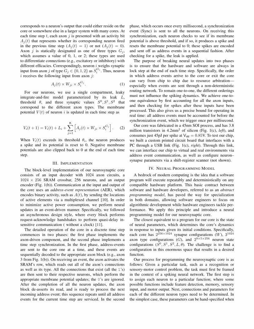
corresponds to a neuron’s output that could either reside on thecore or somewhere else in a larger system with many cores. Ateach time step t, each axon j is presented with an activity bitAj(t) that represents whether its corresponding neuron firedin the previous time step (Aj(t) = 1) or not (Aj(t) = 0).Axon j is statically designated as one of three types Gj ,which assumes a value of 0, 1, or 2; these types are usedto differentiate connections (e.g., excitatory or inhibitory) withdifferent efficacies. Correspondingly, neuron i weighs synapticinput from axon j of type Gj ∈ {0, 1, 2} as SGj

i . Thus, neuroni receives the following input from axon j:

Aj(t)×Wji × SGj

i . (1)

For our neurons, we use a single compartment, leakyintegrate-and-fire model parameterized by its leak L,threshold θ, and three synaptic values S0, S1, S2 thatcorrespond to the different axon types. The membranepotential V (t) of neuron i is updated in each time step as

Vi(t+ 1) = Vi(t) + Li +

K∑j=1

[Aj(t)×Wji × S

Gj

i

]. (2)

When Vi(t) exceeds its threshold θi, the neuron producesa spike and its potential is reset to 0. Negative membranepotentials are also clipped back to 0 at the end of each timestep.

III. IMPLEMENTATION

The block-level implementation of our neurosynaptic coreconsists of an input decoder with 1024 axon circuits, a1024 × 256 SRAM crossbar, 256 neurons, and an outputencoder (Fig. 1(b)). Communication at the input and output ofthe core uses an address-event representation (AER), whichencodes binary activity, such as A(t), by sending the locationsof active elements via a multiplexed channel [10]. In orderto minimize active power consumption, we perform neuralupdates in an event-driven manner. Specifically, we followedan asynchronous design style, where every block performsrequest-acknowledge handshakes to perform quasi-delay in-sensitive communication ( without a clock) [11].

The detailed operation of the core in a discrete time stepcommences in two phases: the first phase implements theaxon-driven component, and the second phase implements atime step synchronization. In the first phase, address-eventsare sent to the core one at a time, and these events aresequentially decoded to the appropriate axon block (e.g., axon3 from Fig. 1(b)). On receiving an event, the axon activates theSRAM’s row, which reads out all of the axon’s connectionsas well as its type. All the connections that exist (all the 1’s)are then sent to their respective neurons, which perform theappropriate membrane potential updates; the 0’s are ignored.After the completion of all the neuron updates, the axonblock de-asserts its read, and is ready to process the nextincoming address event; this sequence repeats until all addressevents for the current time step are serviced. In the second

phase, which occurs once every millisecond, a synchronizationevent (Sync) is sent to all the neurons. On receiving thissynchronization, each neuron checks to see if its membranepotential is above threshold, and if so, it produces a spike andresets the membrane potential to 0; these spikes are encodedand sent off as address events in a sequential fashion. Afterchecking for a spike, the leak is applied.

The purpose of breaking neural updates into two phasesis to ensure that the hardware and software are always inlock step at the end of each time step. Specifically, the orderin which address events arrive to the core or exit the corecan vary from chip to chip due to resource arbitration—especially when events are sent through a non-deterministicrouting network. To remain one-to-one, the different orderingsmust not influence the spiking dynamics. We achieve one-to-one equivalence by first accounting for all the axon inputs,and then checking for spikes after these inputs have beenprocessed. This also gives us a precise bound for operating inreal time: all address events must be accounted for before thesynchronization event, which we trigger once per millisecond.

Our core was fabricated in a 45nm SOI process, and has 3.8million transistors in 4.2mm2 of silicon (Fig. 1(c), left), andconsumes just 45pJ per spike at Vdd = 0.85V. To test our chip,we built a custom printed circuit board that interfaces with aPC through a USB link (Fig. 1(c), right). Through this link,we can interface our chip to virtual and real environments viaaddress event communication, as well as configure neuron–synapse parameters via a shift-register scanner (not shown).

IV. NEURAL PROGRAMMING MODEL

A bedrock of modern computing is the idea that a softwareprogram will execute repeatably and deterministically on anycompatible hardware platform. This basic contract betweensoftware and hardware developers, referred to as an abstractprogramming model, has paved the way for specializationin both domains, allowing software engineers to focus onalgorithmic development while hardware engineers tackle per-formance. We apply this principle and introduce a neuralprogramming model for our neurosynaptic core.

The closest equivalent to a program for our core is the stateof neural parameters, which determines the core’s dynamicsin response to inputs given its initial conditions. Specifically,each core has 2256×1024 synapse configurations (W ), 31024

axon type configurations (G), and 29×5×256 neuron stateconfigurations (S0, S1, S2, L, θ). The challenge is to find aconfiguration in this enormous space that results in a desiredfunction.

Our process for programming the neurosynaptic core is asfollows: Given a particular task, such as a recognition orsensory-motor control problem, the task must first be framedin the context of a spiking neural network. The first step isto assign each neuron to a particular function; where somepossible functions include feature detection, memory, sensoryinput, and motor output. Next, connections and parameters foreach of the different neuron types need to be determined. Inthe simplest case, these parameters can be hand-specified when

Name Description Range

Wji Connection

between axon

j and neuron i

0,1

Gj Axon type 0,1, 2

Si0..2 Synapse

values

-256

to 255

Li Leak -256

to 255

i Threshold 1 to

256

K A

xo

ns

N Neurons

K N Synapses

Wji Gj

Si0..2

Li

i

(a)

A3

A2

A1

AK

De

co

de

… A1 , A3

Input spikes

1

0

1

0

time

dt

Axo

n A

ctivity A

(t)

Axons

N1 N2 N3 NM

Ne

uro

ns

Crossbar Synapses Type

GK

G3

N1 N1 N3 N3 NM M NM

1 0 1 1

N1

N2 …

Select & Encode

Output spikes

G2

G1

Sync

(b)

2mm

3m

m

256 Neurons

10

24

Axo

ns

1024x256

Synapses

Core CPLD

Spikes Out

Axons from

USB

Spikes to

USB

Spikes In

(c)

Fig. 1. (a) The core consists of axons, represented as rows; dendrites, represented as columns; synapses, represented as row–column junctions; and neuronsthat receive inputs from dendrites. The parameters that describe the core have integer ranges as indicated. (b) Internal blocks of the core include axons (A),crossbar synapses implemented with SRAM, axon types (G), and neurons (N). An incoming address event activates axon 3 (A3), which reads out that axon’sconnections, and results in updates for neurons N1, N3 and NM. (c) left Neurosynaptic die measure 2mm × 3mm including the I/O pads. right Test boardthat interfaces with the chip via a USB 2.0 link. Spike events are sent to a PC for data collection, and are also routed back to the chip to implement recurrentconnectivity.

the function is straightforward. For more complex functions,the parameters need to be learned offline, typically throughan optimization procedure on a representative dataset froma real or virtual environment. Finally, these parameters aretransformed into a hardware-compatible format, where theycan be downloaded to the hardware platform and tested inreal-time.

To demonstrate our neural programming framework, wedescribe four example applications that have been mappedto our hardware in the following subsections. Results werecollected from our custom chip via the PC-USB interface,while using the host PC for graphics display, user interface,and supporting software as necessary. We also verified for anumber of test cases that each application operated exactly aspredicted by the software model. Detailed information on thespecific parameter values used for each example can be foundin the appendix.

A. Autonomous Virtual Robot Driver

For our first application, we programmed the neurosynapticcore to steer a simulated robot around a virtual racetrack. Thegoal of the robot driver application is to keep the robot on the

racetrack using an autonomous, closed-loop control system.The virtual robot is a physics based emulation of the real-life MobileRobots Pioneer 3-AT (P3AT), a four wheel driverobotic platform with a vision sensor. We defined a clover-shaped racetrack in the Unreal Tournament 3 virtual environ-ment. The autonomous control system receives visual inputfrom its camera, and controls the robot by issuing differentialwheel speed commands to the left and right wheels. Fig. 2(a)shows screenshots of the view seen by the robot camera andthe robot on the racetrack in the virtual environment.

Controlling the P3AT robot in the virtual environmentrequires two key components: vision to see the racetrack anda control system to direct the robot’s actions. In the virtualenvironment, we simplified the vision task of detecting theroad by performing preprocessing on the host computer, andfocused on implementing the control system on the hardware.

We program the neurosynaptic core to implement a negativeproportional feedback controller in which difference in powerapplied to the left and right wheels is proportional to thedifference in the P3AT’s direction of travel and the directionto the center of the road (in visual space). Therefore, when theP3AT drives down the center of the road both wheels receive

(a) Virtual Environment (b) System Block Diagram

0 50 100 150 200 250

50

100

150

200

250

time (ms)

neur

on in

dex

0 0.2 0.4 0.6 0.8 10

0.5

1

1.5

fraction of neurons enabledmea

n di

stan

ce to

cen

ter

(c) Results

Fig. 2. (a) Screenshots of the robot-eye view in the virtual environment at top and the simulated P3AT robot on the racetrack at bottom. (b) Autonomousrobot control system block diagram. (c) top Spike activity of network during driving task. bottom Average distance from center of driving track, as a functionof the number of neurons used where distance saturates at 2.0 in failed trials.

equal power. The system is a self-contained closed loop, and ablock diagram is shown in Fig. 2(b). Vision processing consistsof a layer of “On” feature detectors that spike when the road iswithin their receptive field. Note that this feature layer couldbe augmented with many other features (e.g., “Off” features,edges, road color statistics, etc.) for a more complex visualprocessing system, which would be necessary in more realisticenvironments. The neurons in the sensory layer, which residein the neurosynaptic core, are driven from these feature layerdetectors to essentially form road detectors that represent theposition of the road in the visual field. The motor commandprocessing block integrates the spiking output from the sensorylayer and produces two values, one for both of the left andright wheels to steer the robot. The power to each wheel isproportional to the number of spikes on each side of the visualfield; therefore, if the road is left of center the left wheelreceives greater power, causing a turn to the left, centeringthe position of the road in the visual scene.

We program the neurosynaptic core as follows, mapping thesensory neuron layer to the hardware. There are 512 “On”-features, which are mapped to 1024 axons, half excitatory andhalf inhibitory. The 256 neurons are then divided up acrossthe visual field, centered at uniform intervals and each takinginput from 32 excitatory and 16 inhibitory axons. The roaddetectors are excitatory in the center (S0 = +2), inhibitory onthe edges (S1 = −2), and zero elsewhere, forming a matchedfilter that fires maximally when the road is centered in thefilter’s receptive field.

We measured the robustness of our neural controller byvarying the fraction of neurons enabled(from 10 to 100%)and tracking the average distance the robot deviated from thecenter of the track (Fig. 2c). Using 100% of the neurons,the performance is near perfect (low mean-squared error), anddegrades smoothly with decreasing percentage of neurons.

B. Pong Player

For our second example, we simulated the classic videogame of Pong and implemented an autonomous player that iscontrolled by the neurosynaptic core. The goal of Pong is tokeep a moving ball contained in a 2D box, where one wallof the box is open such that the ball must be hit by a paddlecontrolled by a player. To make the game more challengingthe direction of the ball is randomly perturbed when it bouncesoff the wall opposite to the paddle. Because the ball movesfaster than the paddle, the challenge for the player is to predictthe correct paddle position far enough in advance.

To implement an autonomous player, the neural networkinteracts with the game the same way a normal player would,through visual access to the ball’s position and a 1D paddlecontroller but without access to precise ball position, velocity,and kinematics that virtual players typically have. The playingarea is divided into a 16 × 14 grid corresponding to visualreceptive fields of 224 neurons that are direction selective,spiking only when the ball moves towards the virtual player’sside of the field (loosely based on the fly visual system [12]).For paddle-control, we assign 14 motor neurons to controla joystick (inertial controller), which moves the paddle’slocation toward the position of the most active motor neuron.

We implement the player with a spiking neural networkusing three subsystems: sensory, reset, and motor. The functionof the sensory neurons is to store the ball’s trajectory as a traceof neural activity (Fig. 3(b-c)). Specifically, sensory neuronsbecome active when the ball moves across the game area,and remain active without external input via excitatory self-connections (autapses). To reset the persistent activity betweenvolleys, the sensory neurons receive strong inhibition froman interneuron when the ball reaches the paddle, and thesensory neurons remain inhibited until the ball reaches thebottom row of the playing area (shutoff by a second inhibitoryinterneuron).

Finally, to associate ball trajectories with the appropriate

0 0.1 0.2 0.3 0.4 0.50.7

0.75

0.8

0.85

0.9

0.95

1

∆V − velocity increments

Perf

orm

ance

a b

paddle side

sensory neurons c

d

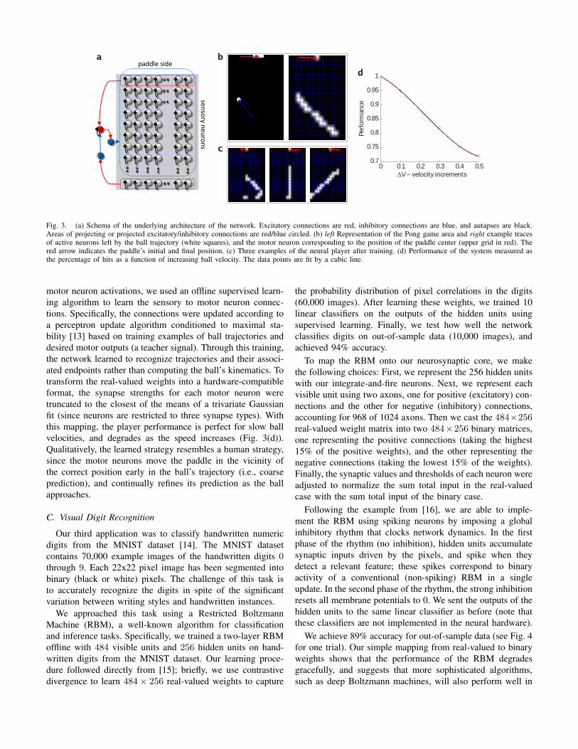
Fig. 3. (a) Schema of the underlying architecture of the network. Excitatory connections are red, inhibitory connections are blue, and autapses are black.Areas of projecting or projected excitatory/inhibitory connections are red/blue circled. (b) left Representation of the Pong game area and right example tracesof active neurons left by the ball trajectory (white squares), and the motor neuron corresponding to the position of the paddle center (upper grid in red). Thered arrow indicates the paddle’s initial and final position. (c) Three examples of the neural player after training. (d) Performance of the system measured asthe percentage of hits as a function of increasing ball velocity. The data points are fit by a cubic line.

motor neuron activations, we used an offline supervised learn-ing algorithm to learn the sensory to motor neuron connec-tions. Specifically, the connections were updated according toa perceptron update algorithm conditioned to maximal sta-bility [13] based on training examples of ball trajectories anddesired motor outputs (a teacher signal). Through this training,the network learned to recognize trajectories and their associ-ated endpoints rather than computing the ball’s kinematics. Totransform the real-valued weights into a hardware-compatibleformat, the synapse strengths for each motor neuron weretruncated to the closest of the means of a trivariate Gaussianfit (since neurons are restricted to three synapse types). Withthis mapping, the player performance is perfect for slow ballvelocities, and degrades as the speed increases (Fig. 3(d)).Qualitatively, the learned strategy resembles a human strategy,since the motor neurons move the paddle in the vicinity ofthe correct position early in the ball’s trajectory (i.e., coarseprediction), and continually refines its prediction as the ballapproaches.

C. Visual Digit Recognition

Our third application was to classify handwritten numericdigits from the MNIST dataset [14]. The MNIST datasetcontains 70,000 example images of the handwritten digits 0through 9. Each 22x22 pixel image has been segmented intobinary (black or white) pixels. The challenge of this task isto accurately recognize the digits in spite of the significantvariation between writing styles and handwritten instances.

We approached this task using a Restricted BoltzmannMachine (RBM), a well-known algorithm for classificationand inference tasks. Specifically, we trained a two-layer RBMoffline with 484 visible units and 256 hidden units on hand-written digits from the MNIST dataset. Our learning proce-dure followed directly from [15]; briefly, we use contrastivedivergence to learn 484× 256 real-valued weights to capture

the probability distribution of pixel correlations in the digits(60,000 images). After learning these weights, we trained 10linear classifiers on the outputs of the hidden units usingsupervised learning. Finally, we test how well the networkclassifies digits on out-of-sample data (10,000 images), andachieved 94% accuracy.

To map the RBM onto our neurosynaptic core, we makethe following choices: First, we represent the 256 hidden unitswith our integrate-and-fire neurons. Next, we represent eachvisible unit using two axons, one for positive (excitatory) con-nections and the other for negative (inhibitory) connections,accounting for 968 of 1024 axons. Then we cast the 484×256real-valued weight matrix into two 484×256 binary matrices,one representing the positive connections (taking the highest15% of the positive weights), and the other representing thenegative connections (taking the lowest 15% of the weights).Finally, the synaptic values and thresholds of each neuron wereadjusted to normalize the sum total input in the real-valuedcase with the sum total input of the binary case.

Following the example from [16], we are able to imple-ment the RBM using spiking neurons by imposing a globalinhibitory rhythm that clocks network dynamics. In the firstphase of the rhythm (no inhibition), hidden units accumulatesynaptic inputs driven by the pixels, and spike when theydetect a relevant feature; these spikes correspond to binaryactivity of a conventional (non-spiking) RBM in a singleupdate. In the second phase of the rhythm, the strong inhibitionresets all membrane potentials to 0. We sent the outputs of thehidden units to the same linear classifier as before (note thatthese classifiers are not implemented in the neural hardware).

We achieve 89% accuracy for out-of-sample data (see Fig. 4for one trial). Our simple mapping from real-valued to binaryweights shows that the performance of the RBM degradesgracefully, and suggests that more sophisticated algorithms,such as deep Boltzmann machines, will also perform well in

22 x 22 Visible Units

968 Axons x 256 Neurons 10 Label Neurons

Axo

ns

Synapses

Input

Predicted: 3

+

-

Per

cent

age

Cor

rect

Digits (a) (b)

Fig. 4. (a) Pixels that represent visible units drive spike activity on excitatory (+) and inhibitory (-) axons to stimulate a 16 × 16 grid of neurons on thechip. Here, spikes are indicated as black squares, and encode the digit as a set of features. The spikes are sent to an off-chip linear classifier that predicts 3as the most likely digit, whereas 6 is the least likely. (b) Measured performance for each digit for out-of-sample data (points), and the average performance(red line) is 89%.

hardware despite low precision synaptic weights.

D. Autoassociation

Our fourth application was storing and recalling patternsin a manner that allows a subset of a pattern to retrieve thewhole. The challenge of this autoassociation task is storingpatterns implicitly in synaptic weights such that they can berecalled with fidelity. We approach autoassociation in twodistinct ways, one with a sparse version of the classic HopfieldNetwork and the other with a two-layer spiking network(Fig. 5).

The Hopfield Network is a classic neural network, whichrealizes autoassocative memory in a recurrently connectednetwork by increasing connection strengths between correlatedneurons while decreasing strengths between anticorrelatedneurons across stored memory patterns. We select a sparseHopfield implementation, storing m binary patterns of lengthn = 256 each with 8 1s (sparsity γ = 8/256) [17], [18]. Sucha sparse implementation is less sensitive to low precision(binary) weights while maintaining a high memory capacity.We trained the network offline, computing real-valuedconnection strengths from neuron j to neuron i with theHopfield Rule given by:

Wji =

m∑k=1

(vkjγ− 1

)(vkiγ− 1

)

where vkj and vki are the stored states of the jth and ith neuronsin pattern k.

We mapped the real-valued synaptic strengths to the binaryneurosynaptic core using the same procedure that we usedfor the RBM (Section 4.3): We imposed a global inhibitoryrhythm that clocks neuron dynamics; we binarized the weightmatrix (Wij) by using two axons for each neuron’s recurrentconnections, setting postive weights to one on a positive axon(S0

i > 0) and the rest to one on a negative axon (S1i < 0)

and setting S0i , S1

i such that the sum total of excitation and

inhibition were preserved. Then, we set all neurons’ thresholds(θi = 1) so that any net excitation caused a neuron to spike,signalling the recall of a 1.

We tested the Hopfield Network’s capacity, the numberof patterns it can store, as well as its completion, how wellit recalls stored patterns. To test capacity, we activated eachpattern in its entirety (10 sets of patterns) and after 10 timesteps observed similarity between the final state and storedpattern, given by the overlap:

β =1

n

n∑i=1

(pi − γ)(vi − γ)/γ/(1− γ)

where p is the original pattern, and v is the network state. Wefound that for few patterns stored (α = m/n < 0.6) patternswere well maintained, with β ≈ 1; as more patterns werestored, storage degraded, with with β decreasing further below1 as the number of stored patterns increased (Fig. 5(b)). Wetested the network’s completion by activating half the 1s ineach pattern (β = 0.5) and observing how the pattern overlapβ changed. For few patterns stored (α < 0.6), patterns werefaithfully recalled; β increased to ≈ 1. As the number ofpattern stored increased (0.6 < α < 1.0), the network statemoved closer to stored patterns but did not consistently recallfull patterns; β increased above 0.5 but did not reach 1. Asthe number of pattern stored was further increased (α > 1.0),the network state moved further from the stored patterns; βdecreased below 0.5, degrading from the partially activatedpattern.

In a similar manner to the Hopfield network, we imple-mented autoassociative pattern recall in a two-layer spikingnetwork. The two-layer spiking network stores patterns in theconnections between two excitatory layers of neurons [19].The first layer, E1, acts as both the input and output. Whenactivated, E1 neurons drive the second layer, E2, activatingonly the neuron(s) most selective to the input, ensured bywinner-take-all inhibition mediated by a neuron in layer I(Fig. 5(c)). Through reciprocal connections, activity in E2

(a)

0 1 20

0.5

1

α, patterns / neurons

β, o

verla

p(b)

E1

...

E2 I

...

......

(c)

presentedstored recalled

pa

tte

rn 1

pa

tte

rn 2

pa

tte

rn 3

(d)

Fig. 5. (a) The Hopfield Network stores patterns in a recurrent weight matrix. (b) When the ratio of patterns to neurons (α) increases, when initializedto the stored patterns (black), overlap (β) decreases. When initialized to stored patterns with half of the ones dropped (gray), the overlap increases. (c) Thetwo-layer network (E1 and E2) stores patterns in reciprocal connections between the excitatory layers. (d) When presented with stored patterns with half ofthe ones dropped, the network restores the patterns.

drives recall of all E1 neurons in the original pattern. In asystem with 121 neurons in both E1 and E2, we stored 121patterns consisting of 8 randomly selected E1 neurons. Thepatterns were learned offline by initializing weights betweenE1 and E2 to 0, then assigning each pattern to a unique E2neuron and setting the weights between that E2 neuron and thepattern in E1 to 1. To test completion, we activated half theE1 neurons in a pattern each with probability 0.1 per step for50 time steps (20 trials per pattern). The two-layer networkshowed 0.995 correct hit rate, and 0.011 false positive rate(Fig. 5(d)).

V. DISCUSSION

A long standing goal of the neuromorphic community is tobuild compact, scalable, and power-efficient neural hardwarethat is supported by a corresponding software environment.Two recent notable projects with similar aims are PyNN [20]and the SpiNNaker project [21]. Our breakthrough neurosy-naptic core is the first of its kind in working silicon to inte-grate neurons, dense synapses, and communication on chip,leading to ultra-low active power in a dense technology, whilesimultaneously demonstrating one-to-one correspondence witha determinstic neural programming model.

As we look forward to building multicore chips with tens ofthousands of neurons and millions of synapses, the challengebecomes searching the astronomic parameter space to find aconfiguration that achieves a desired neural function. In thecurrent neural programming model, our approach is to learnparameters offline where any optimization technique can beused (i.e., the algorithm may or may not be neural inspired).An alternative approach is to integrate learning into the neuralhardware itself (e.g., using spike timing-dependent plasticity),allowing connections to be updated during run time (see [22],[23] for examples). This approach, however, is limited tolearning rules that are efficient to implement in hardware.We believe that a hybrid of these two approaches is the best,similar to evolutionary biology: nature provides a hardwiredscaffold, while nurture allows for online adaptation.

APPENDIX ANEURAL PROGRAMS (SOURCE)

The neurosynaptic core is defined as the set of parameters:

{Wji, Gj , SGj

i , Li, θi}

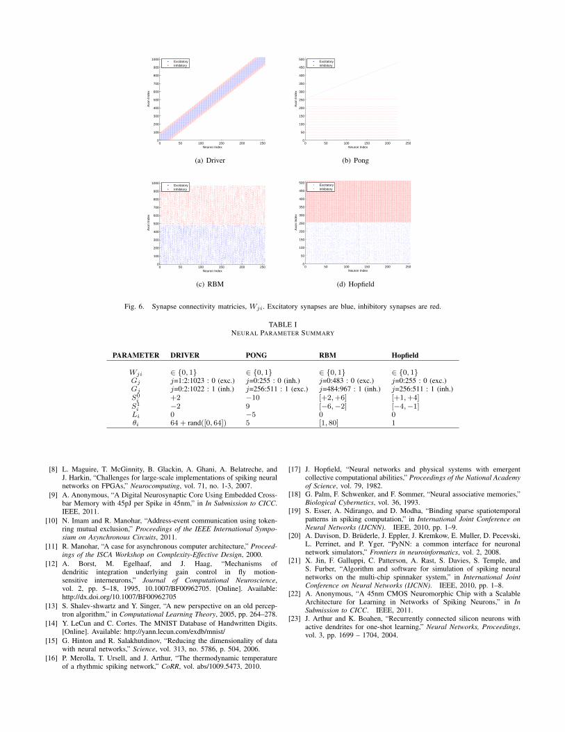
For each of the four demos, the neural parameter values usedto program each application, are listed in Table I. The synapticconnectivity matrix Wji, is shown in Fig. 6.

ACKNOWLEDGMENT

This research was sponsored by DARPA under contractNo. HR0011-09-C-0002. The views and conclusions containedherein are those of the authors should not be interpreted asrepresenting the official policies, either expressly or implied,of DARPA or the U.S. Government. Authors thank Sue Gilson,Greg Corrado, Scott Hall, Kavita Prasad, Scott Fairbanks,Jon Tse, Ben Hill, Robert Karmazin, and Carlos Ortega fortheir contributions. Approved for Public Release, DistributionUnlimited.

REFERENCES

[1] C. Mead, Analog VLSI and neural systems. Addison-Wesley, 1989.[2] K. Boahen, “Neurogrid: emulating a million neurons in the cortex,”

in IEEE international conference of the engineering in medicine andbiology society, 2006.

[3] G. Indiveri, E. Chicca, and R. Douglas, “A VLSI array of low-powerspiking neurons and bistable synapses with spike-timing dependentplasticity,” IEEE Transactions on Neural Networks, vol. 17, no. 1, pp.211–221, 2006.

[4] A. Montalvo, R. Gyurcsik, and J. Paulos, “Building blocks for atemperature-compensated analog vlsi neural network with on-chip learn-ing,” in IEEE International Symposium on Circuits and Systems (ISCAS),vol. 6, 1994, pp. 363–366.

[5] R. Ananthanarayanan, S. Esser, H. Simon, and D. Modha, “The cat isout of the bag: cortical simulations with 109 neurons, 1013 synapses,”in Proceedings of the Conference on High Performance ComputingNetworking, Storage and Analysis. ACM, 2009, p. 63.

[6] B. Shi, E. Tsang, S. Lam, and Y. Meng, “Expandable hardware for com-puting cortical feature maps,” in Proceedings of the IEEE InternationalSymposium on Circuits and Systems (ISCAS). IEEE, 2006.

[7] J. M. Nageswaran, N. Dutt, J. L. Krichmar, A. Nicolau, and A. Vei-denbaum, “Efficient simulation of large-scale spiking neural networksusing cuda graphics processors,” in Proceedings of the InternationalJoint Conference on Neural Networks (IJCNN). IEEE, 2009, pp. 3201–3208.

0 50 100 150 200 2500

100

200

300

400

500

600

700

800

900

1000

Neuron IndexA

xon

Inde

x

ExcitatoryInhibitory

(a) Driver

0 50 100 150 200 2500

50

100

150

200

250

300

350

400

450

500

Neuron Index

Axo

n In

dex

ExcitatoryInhibitory

(b) Pong

0 50 100 150 200 2500

100

200

300

400

500

600

700

800

900

1000

Neuron Index

Axo

n In

dex

ExcitatoryInhibitory

(c) RBM

0 50 100 150 200 2500

50

100

150

200

250

300

350

400

450

500

Axo

n In

dex

Neuron Index

ExcitatoryInhibitory

(d) Hopfield

Fig. 6. Synapse connectivity matricies, Wji. Excitatory synapses are blue, inhibitory synapses are red.

TABLE INEURAL PARAMETER SUMMARY

PARAMETER DRIVER PONG RBM Hopfield

Wji ∈ {0, 1} ∈ {0, 1} ∈ {0, 1} ∈ {0, 1}Gj j=1:2:1023 : 0 (exc.) j=0:255 : 0 (inh.) j=0:483 : 0 (exc.) j=0:255 : 0 (exc.)Gj j=0:2:1022 : 1 (inh.) j=256:511 : 1 (exc.) j=484:967 : 1 (inh.) j=256:511 : 1 (inh.)S0i +2 −10 [+2,+6] [+1,+4]S1i −2 9 [−6,−2] [−4,−1]Li 0 −5 0 0θi 64 + rand([0, 64]) 5 [1, 80] 1

[8] L. Maguire, T. McGinnity, B. Glackin, A. Ghani, A. Belatreche, andJ. Harkin, “Challenges for large-scale implementations of spiking neuralnetworks on FPGAs,” Neurocomputing, vol. 71, no. 1-3, 2007.

[9] A. Anonymous, “A Digital Neurosynaptic Core Using Embedded Cross-bar Memory with 45pJ per Spike in 45nm,” in In Submission to CICC.IEEE, 2011.

[10] N. Imam and R. Manohar, “Address-event communication using token-ring mutual exclusion,” Proceedings of the IEEE International Sympo-sium on Asynchronous Circuits, 2011.

[11] R. Manohar, “A case for asynchronous computer architecture,” Proceed-ings of the ISCA Workshop on Complexity-Effective Design, 2000.

[12] A. Borst, M. Egelhaaf, and J. Haag, “Mechanisms ofdendritic integration underlying gain control in fly motion-sensitive interneurons,” Journal of Computational Neuroscience,vol. 2, pp. 5–18, 1995, 10.1007/BF00962705. [Online]. Available:http://dx.doi.org/10.1007/BF00962705

[13] S. Shalev-shwartz and Y. Singer, “A new perspective on an old percep-tron algorithm,” in Computational Learning Theory, 2005, pp. 264–278.

[14] Y. LeCun and C. Cortes. The MNIST Database of Handwritten Digits.[Online]. Available: http://yann.lecun.com/exdb/mnist/

[15] G. Hinton and R. Salakhutdinov, “Reducing the dimensionality of datawith neural networks,” Science, vol. 313, no. 5786, p. 504, 2006.

[16] P. Merolla, T. Ursell, and J. Arthur, “The thermodynamic temperatureof a rhythmic spiking network,” CoRR, vol. abs/1009.5473, 2010.

[17] J. Hopfield, “Neural networks and physical systems with emergentcollective computational abilities,” Proceedings of the National Academyof Science, vol. 79, 1982.

[18] G. Palm, F. Schwenker, and F. Sommer, “Neural associative memories,”Biological Cybernetics, vol. 36, 1993.

[19] S. Esser, A. Ndirango, and D. Modha, “Binding sparse spatiotemporalpatterns in spiking computation,” in International Joint Conference onNeural Networks (IJCNN). IEEE, 2010, pp. 1–9.

[20] A. Davison, D. Bruderle, J. Eppler, J. Kremkow, E. Muller, D. Pecevski,L. Perrinet, and P. Yger, “PyNN: a common interface for neuronalnetwork simulators,” Frontiers in neuroinformatics, vol. 2, 2008.

[21] X. Jin, F. Galluppi, C. Patterson, A. Rast, S. Davies, S. Temple, andS. Furber, “Algorithm and software for simulation of spiking neuralnetworks on the multi-chip spinnaker system,” in International JointConference on Neural Networks (IJCNN). IEEE, 2010, pp. 1–8.

[22] A. Anonymous, “A 45nm CMOS Neuromorphic Chip with a ScalableArchitecture for Learning in Networks of Spiking Neurons,” in InSubmission to CICC. IEEE, 2011.

[23] J. Arthur and K. Boahen, “Recurrently connected silicon neurons withactive dendrites for one-shot learning,” Neural Networks, Proceedings,vol. 3, pp. 1699 – 1704, 2004.