1

Buckling of fibres and yarns within ropes and other fibre assemblies

R.E. Hobbs*, M.S. Overington, J.W.S. Hearle and S.J. Banfield

Tension Technology International Ltd, TTI House, Preston PR1 3NA, UK

* Address for correspondence: Department of Civil Engineering, Imperial College, LondonSW7 2BU, UK

Individual yarns within ropes can be subject to axial compression even though the ropeas a whole is under tension. This leads to buckling in sharp kinks and then to failure byaxial compression fatigue after repeated cycling. An existing elastic theory, whichapplies to heated pipelines subject to lateral and axial restraint, predicts alternativemodes of either continuous buckling or intermittent buckled zones alternating with slipzones. The mechanics of axially compressed yarns within ropes are similar, but thetheory has been extended to cover plastic deformation at hinge points. The predictedform of groups of saw-tooth buckles, which curve at the ends of the zones into the sliplengths, is in agreement with observed effects. Numerical calculation gives quantitativepredictions in agreement with experimental results, despite uncertainty about thecorrect values for bending stiffness and plastic yield moment, depending on whether theyarns act as solid rods or freely slipping fibre assemblies.

1 INTRODUCTION

Fibre and wire ropes are primarily intended for service as tensile elements, but failure mayresult from axial compression of parts of the cross-section, namely individual fibres, yarns orstrands, while the bulk of the rope is safely in tension. Similar effects may occur in othertextile structures, such as carpets or industrial woven fabrics. If the axial compression leadsto a mild rounded buckling, as in an elastic deformation, there will be little damage, but if, asoften happens, plastic yielding leads to sharp kinks, then fibres will fail in repeated cycling. In ropes, axial compression of individual components can arise from a number of causesincluding:

C Bending. If a rope under tension passes over a sheave (pulley) or is taken round anyother solid object with too small a radius, components inside the curve may be putinto compression. Ropes may also buckle into bent forms or, at low or zero tension,be forced to bend by transverse forces.

C Rope twisting. If a parallel assembly of fibres is twisted in either direction at constantlength, the outer layers are forced into longer paths and so develop tension. If theoverall rope tension falls below the value developed in this way, the rope will contractand the central fibres will be put into compression. In a simple twisted structure, anincrease of twist will cause the central straight components to go into compression,whereas a decrease of twist will compress the outer components. In morecomplicated rope structures, with twist at several levels, the precise effects willdepend on the geometry, but twisting will always force some components into axialcompression in the absence of sufficient overall rope tension.

2

Twisting in tension-tension cycling can develop for two reasons. If the rope is nottorque-balanced, tension will cause a torque to develop, and this can lead to the ropetwisting against a soft termination, such as a splice, or against other line components. Similarly, if other line components, such as connecting wire ropes, are not torque-balanced, twist may be transmitted to the fibre rope. Alternatively, if there isnonuniformity along the rope, different sections of rope will twist against each other. All of these effects have been found in practice.

Buckling into three-dimensional curved paths also gives rise to twist.

C Length imbalance. If, as a result of manufacture or subsequent handling and use, oneor more components of a rope is longer (parallel to the axis of the rope) at zerotension than the other components, then the equilibrium state of the entire rope at zerotension will have the longer components in compression and the shorter ones intension. A critical positive tension is needed to eliminate axial compression in thelonger elements.

Similar effects can clearly arise in umbilicals, armoured electrical and optical cables, andhoses. Indeed, the wider range of elemental properties in some of these products may makesensitive elements such as optical fibres more rather than less likely to be put intocompression.

Compression by itself is not usually a major problem, rather it is the response tocompression, and how often this response is repeated which is of concern. If a rope as awhole is subject to an axial compressive force, it will buckle into a smooth curve with aradius that is too large to cause fibre damage. The only exceptions would be for very shortlengths of rope or where a rope is restrained from buckling by a lateral pressure. Thecommon damaging situation is when a component within a rope is forced into compressionwhile subject to the restraint of neighbouring components, such as a sheave, or other ropecomponents which are still under tension. In high strength fibre ropes, this restrainedbuckling of the compressed element is known as kinking, and is a form of elasto-plasticbuckling of the fibre or group of fibres against the restraint afforded by the neighbouringelements which are still in tension.

Kinking due to axial compression is a phenomenon that occurs on many scales frommountain ranges to oriented polymer molecules. In fibres, the effects at the molecular levelare shown by the presence of kinkbands, which run across the fibres at about 45E, whenfibres are uniformly compressed, or, more commonly, on the inside of bends. Repeatedflexing of fibres leads to failure, either due to breakdown along kinkbands or to axial splittingfrom the accompanying shear stresses. As described by Hearle et al (1998), these forms offailure have been observed in laboratory flex tests and in ropes and carpets after cyclicloading. In typical test conditions, failure may occur in around 1000 cycles in aramid fibres,Hearle and Wong (1977), but polyester and nylon fibres would last longer, Hearle andMiraftab (1991). Data from yarn buckling tests carried out for FIBRE TETHERS 2000(1995), show severe strength loss in aramid yarns after 20,000 cycles, in HMPE yarns after200,000 cycles and in polyester yarns after 1,000,000 cycles.

The first reported engineering failure in an aramid rope due to axial compression fatigue was

3

in the mooring lines for the construction ship Ocean Builder I used in the erection of the Lenatower in the Gulf of Mexico in 1983, Riewald (1986) and Riewald et al (1986). The lineswere deployed on buoys in 1045 feet of water 4-6 weeks before the arrival of the ship. Onrecovering and tensioning, four ropes failed, reportedly at 20% of rated strength. The failurewas very thoroughly investigated and explained in the following way. Torque generated inthe ropes due to wave action led to rotation, causing shear and compressive strains, which inturn led to fibre kinking with an accompanying loss of strength. Laboratory studies andocean deployments, resulting from the investigation of this failure, gave more examples ofkinking occurring due to axial compression. Gross kinks were seen in yarns and severe fibredamage was shown up as strongly dyed bands at regular intervals along the yarns. The studyof this failure led to improved rope constructions and procedures as a way of avoiding axialcompression fatigue.

The occurrence of axial compression fatigue in various types of fibre ropes was found aftertension-tension cycling in the joint industry study, FIBRE TETHERS 2000 (1995). Samplesof these ropes were made available for microscopic examination in the Department ofTextiles at UMIST, with results reported by Hearle et al (1998). The observed effectsincluded the following :

C a wavy buckling of yarns or strands, at fairly low curvature, which would not belikely to cause serious damage to fibres

C kinkbands running across fibres indicating regions of uniform axial compression

C sharp kinks of fibres as a whole, usually occurring cooperatively across yarns

C breaks of fibres along kinkbands within fibres

C axial splits, which would have been caused by fibre bending

Commonly, the sharp fibre kinks, with internal damage that could be picked out by dyeingaramid yarns, occurred in groups in zig-zag sections separated by straight lengths. This, inturn, led to broken pieces, which were a few millimetres in length, followed by unbrokenportions, which were a few centimetres long. Some examples are described later in thispaper.

2. ANALYSIS

2.1 Approach to modelling

The observed failure modes in a rope suggest that an element of a rope fails by bucklingbecause it is carrying an axial compressive load even though it is laterally restrained byadjacent elements carrying tension. The phenomena appear at a number of different scales ina rope : a sub-rope may buckle in a multi-rope assembly, a strand may buckle whilerestrained by adjacent strands, or a yarn fail when restrained by adjacent yarns. It is alsoobserved that the buckles become more severe as the elements get smaller. Ropes andstrands take up gentle, harmless elastic curves, while yarns and particularly the individual

4

y )) % n 2y %m8

(4x 2 & L 2) ' 0 (1)

P ' f(L) (2)

filaments in them form much more deleterious plastic hinges or kinks, kinks which areapparent even at the molecular level. This part of the paper models the buckling of theelement by examining the theory behind the buckling of a semi-infinite beam-columncarrying an axial load whilst laterally supported by other elements. The beam is assumed tobe elastic initially, and then to yield at a known "plastic hinge" moment. Two classes ofbuckles are considered, namely general periodic modes and localised modes, which are moredamaging in practice because of energy inputs from adjacent, unbuckled, areas of the beam. The elastic behaviour of such a beam is, fortunately, fairly well understood because it hasproved to be of economic importance in many other areas. The plastic behaviour has not,apparently, been examined before, and it is developed ab initio here, based on the premisethat it is preceded by elastic buckling, which may be non-damaging in itself but whichtriggers the plastic buckling.

2.2 Elastic Buckling

As noted above, there is a large volume of earlier work on the lateral buckling of long beamsagainst lateral restraint, related to the lateral buckling of railway tracks and, later, submarinepipelines. The lateral restraining force may be elastic, i.e. proportional to the lateraldisplacement, or frictional, i.e. of constant magnitude and opposing further growth ofdeflection.

However, for a linearly elastic lateral restraint only a periodic mode (Mode 4 of Fig.1) ispossible, and the observed presence of localised modes in ropes suggests that the "frictional"or constant force lateral restraint model, where localised modes (Modes 1-4 of Fig.1) arepossible, is a better choice. This view is reinforced by the presence of a radial pressure p onthe buckling element in a rope under tension due to the helical nature of adjacent elements orany braided jacket. This pressure is, to the first order, unaffected by any buckle, and thelateral restraint on unit length of the element is therefore taken as pd, where d is the diameterof the element. The analysis that follows is then very close to that for submarine pipelines byHobbs (1984) and Hobbs and Liang (1989), so that it is only presented in summary here.

In the notation of Fig.2, the governing differential equation for the buckled beam is

where a prime denotes differentiation of the displacement y with respect to the longitudinalcoordinate x, m=pd/EI and n2=P/EI. E is Young's Modulus for the beam, I its effectivesecond moment of area, P the compressive axial load and L the buckle half-wavelength. Thesolution to this differential equation is presented in Hobbs (1984), but proceeds byconsidering the boundary conditions for the various modes, whether localised or periodic,and in each case gives a relationship of the form:

5

mL

o

12

(y ))2 ' (Po & P) LEA (3)

Po ' P % g(L) (4)

Ls ' (Po & P)/(µpπd) (5)

s ' 0.5(Po & P) Ls/EA (6)

The other important element in the analysis is to recognise that as the buckle forms the forcein it drops to maintain displacement compatibility. In the pipeline analysis, and with equalvalidity here, the axial load is displacement controlled rather than force controlled. In thepipeline the axial force is induced by the restraint of thermal expansion, and if (by buckling)the line can take up a slightly longer path the force will be reduced to some extent. Likewise,in the rope the compressive force will be reduced by buckling. Considering the 4 mode first,if the force just before buckling is Po, and falls to P on buckling, displacement compatibilityfor a buckle of length L requires the change in arc length around the buckle to match thegrowth in length due to the force change, or:

where A is the cross-sectional area of the beam.

Using the solution to the differential equation (1), the integral on the left hand side can beevaluated and equation (3) rearranged to yield an equation of form:

Turning to the localised modes, Modes 1-4, equations (2) and (3) will be modified by twofactors. The first is trivial, in that the total length L (measured over the 1 to 4 halfwaves asappropriate) of the buckle should be considered. The second is more basic, and recognisesthat the compatibility condition, equation (3), should be modified to include the influence oftwo 'slipping lengths' adjacent to the localised buckle (Fig.3). The slip lengths form toaccommodate the difference between Po, the force remote from the buckle which isunchanged by the formation of the buckle, and the lower force P, within the buckle itself. The slip length, Ls, is determined by the effective friction between the beam and thesurroundings. If the friction coefficient is µ, and the radial pressure p on a beam of diameterd, or perimeter πd, then:

The slip lengths on either side of the buckle then feed some displacement into the buckle,equal to the average force change in Ls times the length divided by the axial rigidity. Theinward movement s each side is thus:

The compatibility condition, equation (3) becomes:

6

mL

o

12

(y ))2 ' (Po & P) LEA

% 2s

substituting for Ls from equation (5) and for s

mL

o

12

(y ))2 ' (Po & P) LEA

% (Po & P)2/(EAµpπd)

(7)

P ' 4π2EI/L 2 (8)

Po ' P % 4.7050 x 10&5 AE(pd/EI)2 L 6 (9)

y ' 4.4495 x 10&3 pdEI

L 4 (10)

M ' 0.05066 pd L 2 (11)

y ) ' 0.01267 pdL 3/EI (12)

P ' k1EIL 2 (13)

The solutions to this quadratic in (Po-P) for the various localised modes lead to a series ofrelationships similar to equation (4). The details and, more usefully, the results are given inHobbs (1984) and Hobbs and Liang (1989), and re-presented here recognising thecorrespondence (i) between w in Hobbs and Liang (1989) and µpπd here, and (ii) betweenµLw for modes 1-4 in Hobbs and Liang (1989), or φw for the 4 mode in Hobbs (1984) and pdhere.

For the 4 mode:

The maximum amplitude of the buckle

and the maximum bending moment

while the maximum slope

The results for modes 1-4 can be presented in a common format. Taking the half-wavelengthof the most significant part of the buckle as L in each case (Fig.4), and using the constants ofTable I, the reduced axial force within the buckle is given by

Then

7

Po ' P % k3µpπdL 1 % k2AEpdL 5

µπ(EI)2

0.5

&1 (14)

y ' k4 pdL 4/EI (15)

M ' k5 pd L 2 (16)

M ' Mp ' k5 pd L 2 (17)

The maximum amplitude of the buckle

while the maximum moment

Table IConstants for Lateral Buckling Modes

ModeConstants

k1 k2 k3 k4 k5

1234

4

80.764π2

34.0628.20

4π2

6.391 x 10-5

1.743 x 10-4

1.668 x 10-4

2.144 x 10-4

0.51.0

1.2941.608

2.407 x 10-3

5.532 x 10-2

1.032 x 10-2

1.047 x 10-2

4.4495 x 10-3

0.069380.10880.14340.1483

0.050664.7050 x 10-5

2.3 Plastic Buckling

2.3.1 Infinite mode

As noted earlier, it is assumed that elastic buckling defines the shape from which plasticbuckling grows. In particular, the buckle length at which the first plastic hinge forms in thevarious modes can be determined from equation (11) for the 4 mode, or equation (16) formodes 1-4 by putting

8

y ' yp % 0.5Lpθ (18)

Mp ' Ppyp ' P(yp % 0.5Lpθ) (19)

P ' Ppyp /(yp % 0.5Lpθ) (20)

(Pop & Pp) Lp /EA ' ep, say (21)

mL

o0.5(y ))2

where Mp is the fully plastic moment (hinge moment) for the buckling element. Assumingthat such a moment can be calculated for a bundle of filaments, equation (17) defines thebuckle length in the various modes at the onset of plasticity. Given this value of L, denotedLp to flag the onset of plasticity, equations (8)-(10) for the 4 mode, and (13)-(15) for modes1-4 then define the maximum amplitude, yp, the force in the buckle, P p, and the axial forceremote from the buckle, Pop, all at the onset of plasticity as the subscript indicates.

Concentrating first on the periodic 4 mode, it is assumed that following the onset of plasticitythe half-wavelength remains constant at Lp, but the amplitude grows and the waveformchanges to a sawtooth form (Fig.5) because the curvature is concentrated at the hinges.

If the (small) slope of the incremental displacement "sawtooth" is θ, the amplitude (Fig.5)grows from yp to

Since the maximum moment in the elastic curve is Mp and remains constant as the plastic"mechanism" develops, then

It might be noted that the lateral force per unit length, pd, does not appear in equation (19)because it cancels.

Equation (19) may be rearranged to give

In essence, because the amplitude grows while the moment remains constant, the axial loadin the buckle must fall.

A second condition exploits the idea of displacement compatibility which was so importantin the elastic analysis. Just before the onset of plasticity, the force in the buckle is Pp, whichis less than the prebuckling force Pop, so that the length Lp must have extended by

It is also worth recalling that this extension matches the arc length term

The extension, or "endo", changes as the plastic buckle develops and the force changes to P,with which is associated a prebuckling force Po. (Po is none too easy to visualise in the 4

9

e ' (Po & P) Lp /EA (22)

∆e ' e&ep ' 2Lp

2(1&cosθ) ' Lpθ

2/2 (23)

(Po & P) & (Pop & Pp) ' EAθ2/2 (24)

Po ' P % (Pop & Pp) % EAθ2/2 (25)

mode, but in modes 1-4 is the force in the beam well away from the plastic buckle). The newvalue of e is

The change in endo, e-ep, is associated with additional "arc length" effects, which are easy toevaluate for the sawtooth incremental form of Fig.5:

for small θ. Substituting for e and ep, and rearranging

or

Equations (20) and (25) are of practical use, taken with equation (18). Equation (20) definesP as a function of θ, and equation (25) gives Po(θ). Equation (18) allows the results to beplotted as a function of the peak amplitude of the buckle, a parameter which can also be used,Hobbs (1984), to present the elastic results.

2.3.2 Modes 1-4

The approach is to combine the ideas developed for the mode 4 plastic buckling, and theconcepts employed in treating the elastic buckling modes 1-4.

To make progress, it is necessary to make some assumptions concerning the likelyincremental geometry of the various plastic buckling modes. The first assumption is that theplastic buckle lengths are similar to the elastic ones, and the second group of assumptionsconcern the number and location of hinges in the collapse mechanisms (Fig.6), and someother geometric details such as the amplitude ratio in mode 4.

With these assumptions, it is possible to find, for each mode:

(i) equations defining the buckle amplitude analogous to equation (18);(ii) equations analogous to equation (20) for the reduced value of P in the plastic buckle; (iii) equations analogous to equation (23) for ∆e leading to results comparable to a

combination of equations (14) and (25) for the force Po remote from the buckle.

In detail, then, the amplitudes are given by

10

y ' yp % c3 Lp θ (26)

P ' Ppyp/y ' Ppyp/(yp % c3Lpθ) (27)

∆e ' c1Lpθ2 (28)

2∆s ' 2(s&sp) ' (Po&P)2 & (Pop&Pp)2 /(EAµpπd) (29)

∆e ' 2∆s % (Pp&P)Lp/EA (30)

∆e ' 0.983 Lpθ2,

Lp ' 2k3Lp ' 2.588Lp

P ' Ppyp/(yp % 0.5Lpθ)

Po ' P % (Pop&Pp)2 % 0.983Lpθ

2EAµpπd & 2.588Lp(PP&P)µpπd 0.5 (31)

and the force P by

where c3 is a constant given in Table II for the various modes.

The changes in arc length are

where the coefficients c1 are also given in Table II.

As the plastic buckle forms, three effects are apparent:

(i) the load in the buckle drops from Pp to P, while the equilibrium value of the forceremote from the buckle falls from Pop to Po;

(ii) e increases by ∆e (equation (28));(iii) the slip into the buckle increases by ∆s each side or 2∆s in total, where

The incremental compatibility condition then becomes

where the second term on the right hand side represents the incremental extension of thewhole buckle as it develops plastically.

Taking mode 3 as an example:

Substituting these results and equation (29) into equation (30) and rearranging, Po is found asa function of θ

In general, for modes 1-4:

11

Po ' P % (Pop&Pp)2 % c1Lpθ

2EAµpπd & c2Lp(Pp&P)µpπd 0.5 (32)

where the constants c1 and c2 are given in Table II.

Table IIConstants for plastic lateral buckling

ModeConstants

c1 c2=2k3 c3

1234

0.350.6080.9830.830

12

2.5883.216

0.350.3460.50.4

Operationally, for each mode equation (27) defines P as a function of θ, and equation (32)then gives Po(θ). Equation (26) allows the results to be plotted as a function of the amplitudeof the buckle, y.

3. APPLICATION OF MODEL

3.1 Role of imperfections

The general form of the results of the foregoing analysis is summarised in Fig. 7, togetherwith a schematic presentation of the effects of various imperfections in rope lay up. Thefigure shows plots of buckle amplitude against the axial compressive load on a ropecomponent at a position remote from the buckle.

Fig. 7(a) focuses on the purely elastic behaviour, and is indicative of the phenomenaencountered in any of the localised modes, Modes 1-4, which are of greater practicalimportance than the infinite mode. Using equations (14) and (15), the upper curve is thelocus of force and amplitude in an initially perfectly straight rope element in staticequilibrium, an “equilibrium path”. The descending part of this curve, from A to B, consistsof points in unstable equilibrium, while the rising part of the curve is stable. The consequenceis that if a perfect system were brought by some means to a point such as A and released itwould not stay put, but would instead snap dynamically to some position with a much greateramplitude and wavelength such as C. It is not easy to visualise just how a perfectly straightrope element might be made, still less taken up to point A, but in the classical literature inthis field it was widely thought that the minimum of curve AC, point B, represented a forcebelow which buckling could not occur in a perfect axially loaded element. The lowestminimum for modes 1-4 was for some time regarded as a “safe load” (or in thermally loaded

12

beams, equivalently, as a “safe temperature”) for use in design with an appropriate safetymargin.

However, once engineers began to address the effects of the initial imperfections which areinevitably present in real railway tracks and pipelines, it rapidly became clear that the “safetemperature” was a potentially dangerous illusion. This may be seen from the three curvesfrom D1, D2, D3 in Fig. 7(a), where the effects of three different initial amplitudes of buckles,or irregularities, are sketched. All of them erode the “safe load” at B to some extent. The firstcurve indicates the consequences of a small initial misalignment: a curve rising from D1 to apeak at E before falling to a minimum below B before rising again to meet the perfect curveasymptotically near C. The falling part of this curve, too, is unstable, so that an imperfectbeam subjected to a load gradually increasing from zero would only follow path D1 as far asE before suddenly losing stability and snapping to F on the rising part of the curve. Largerimperfections D2 and D3 show respectively a smaller snap at a lower load, and a monotonic(albeit nonlinear) rising behaviour. At large enough amplitudes all of the imperfect curvesconverge asymptotically to the perfect response.

It is certain that the elements of a rope are no more likely than a pipeline or railway track tobe perfectly straight at zero load. As well as any imperfections in the manufacturing process,the helical lay of, say, a core strand will predispose the strand to buckle in different directionswithin a given lay length, while the gaps between the neighbouring strands will inevitablyprovide a lower radial pressure locally than the uniform radial pressure assumed in theanalysis, as well as some space for the core strand to deform into. Thus even before thequestion of the possibility of plastic hinge formation in the strand is addressed it is clear thata strand is likely to be affected by significant initial imperfection effects in the same way asthe pipelines whose analysis suggested this treatment.

Fig. 7(b) outlines some of the possibilities once the formation of plastic hinges is postulated.As the amplitude of buckles increases, so does the maximum bending curvature, which willeventually reach the plastic yield condition. In principal, depending only on the plastic yieldmoment of the yarn or strand under consideration, a plastic hinge could occur at the crest of abuckle at any amplitude, whether small or large. The “perfectly straight case” is representedby the lines from H1, H2, H3, H4. The plastic responses, which are superimposed on thecurve ABC from Fig. 7(a), peel off from the elastic equilibrium path and drop below it,before rising again at rather large amplitudes. It was noted above that the perfect path wouldsnap from A in the elastic case: in the plastic case the snap would be more vigorous becauseit would be to a much larger amplitude than that on the elastic rising path.

The behaviour of the elasto-plastic imperfect system is illustrated in Fig. 7(b) by “snapping”from the curve D1 of Fig. 7(a). Some interesting possibilities arise. Taking hinge formation atthe first of the four amplitudes selected in the perfect case, at H5, plasticity would developwell before E, the peak of the elastic imperfect curve, and cause a snap at once to a ratherlarge amplitude. At this point it is worth recalling that although the amplitude grows in aplastic buckle it has been assumed in the analysis above that the wavelength, defined as it isby the hinge positions, does not change: in this it differs from the elastic analysis whereamplitude growth goes hand in hand with wavelength growth.

13

Prediction of hinge formation at equilibrium positions like H6, H7, H8 would imply that astrand under load increasing steadily from zero would first reach point E. For the cases, H6and H7, it would then start to snap elastically, but, when the critical amplitude was reachedwould peel off the unstable dynamic buckling curve to form hinges at amplitudes H6 and H7,close to those of H2 and H3 respectively. The snap would continue at constant wavelengthtowards the rising part of the plastic equilibrium paths from H6 to H7, joining asymptoticallyaround G. For case H8, there would also be snap at E, but to the elastic line, which would befollowed until the plastic hinge formed at H8, close to H4.

As noted below, buckling in rope yarns has been observed where realistic numerical valuesfor the yarn and fibre properties seem to be consistent with the small amplitude/short half-wavelength formation of plastic hinges. A history like D1 H5 or D1 E with a snap towards G atconstant wavelength would provide a plausible explanation for the observed condition of theyarns.

It is recognised that much of the above discussion is heuristic, but it appears to cast light onphenomena which have been the subject of much debate among the authors. Withoutinformation on the nature of imperfections - and a more complicated theory - it is notpossible to make a prediction of the response based on independent input data. However, theplastic deformation equations can be solved if an arbitrary choice of the amplitude, and hencealso the half-wavelength and slip length, of buckles is made.

3.2 Numerical calculation

A computer program has been written to determine solutions to the equations. Calculationsapplicable to an aramid (Twaron 1000) rope, for which experimental observations are givenin the next section, have been carried out. This rope was tested in tension-tension cycling at38+24% break load. The rope has a “wire-rope construction” with 6 strands round a singlecore strand. Each strand is composed of 6-round-1 rope yarns. The core rope yarns in eachstrand contain 7 “textile” yarns, as supplied by the fibre manufacturer; the outer rope yarns ineach strand contain 5 “textile” yarns. The calculations relate to the core rope yarn of the corestrand. The relevant parameters in SI units, with conversions in brackets are as follows. Thesymbols relate to the rope yarn, which is the basis for the calculation, and the values used inthe computation are put in bold.

FIBRE: linear density = 1.7E-7 (1.7 dtex); density = 1.44E3 (1.44 g/cm3); area = 1.7E-7/1.44E3 = 1.18E-10 (1.18 x 10-4 mm2); diameter = /(4A/π) = /(4 x 1.18E-10 / 3.142) =1.226E-5 (12.26 µm).

“TEXTILE” YARN: 1000 fibres; linear density = 1.7E-4 (1700 dtex); total fibre area =1.18E-7 (0.118 mm2); diameter of equivalent solid rod = /(4 x 1.18E-7 / 3.142) = 3.876E-4(0.3876 mm). Assume packing factor = 0.7: area = 1.68E-7 (0.168 mm2); diameter = /(4 x1.68E-7 / 3.142) = 4.625E-4 (0.46 mm).

ROPE YARN (strand core): 7 “textile” yarns; linear density = 1.19E-3 (1190 tex); total fibrearea = 8.26E-7 (0.826 mm2); diameter of equivalent solid rod = 1.03E-3 (1.03 mm).Assuming packing factor = 0.67: area A = 1.23E-6 (1.23 mm2); diameter d = /(4 x 1.23E-6 /

14

3.142) = 1.25E-3 (1.25 mm), which was the measured diameter.

ROPE: number of “textile” yarns = (7 x 7) in strand cores + (7 x 6 x 5) in strand outers =259; total fibre area = 3.05E-5 (30.5 mm2). Assume packing factor of 0.635: area = 4.80E-5;diameter = /(4 x 4.80E-5 / 3.142) = 7.82E-3 (7.82 mm), which was the measured diameter.

MECHANICAL PROPERTIES: fibre modulus = 7.8E10 (78 GPa); for packing factor of0.67, yarn modulus E = 5.23E10 (52.3 GPa).Fibre yield stress = 5E8 (0.5 GPa); this is the value given by van der Zwaag and Kampschoer(1987) for Twaron; Allen (1987) gives 0.37 GPa for Kevlar. Yarn yield stress (corrected forpacking) fy = 3.35E8 (0.335 GPa). Coefficient of friction µ = 0.15; measurements in FIBRE TETHERS 2000 (1995) gave valuesbetween 0.12 and 0.19.

RADIAL PRESSURE: p = 1E8 (0.1 GPa). The minimum tension in the fatigue testing was14% of break load. The rope has a nominal break load of 5 tonne (50 kN), which, since itcontains 259 yarns, would give a tensile strength of approximately 1.15 GPa and a minimumtensile stress on the rope of approximately 0.16 GPa. This implies that the radial pressurewould equal 63% of the tensile stress. Calculations carried out using a computer programOPTTI-ROPE from TTI Ltd gave values of radial pressure between 0.07 and 0.18 Gpa.

Although there is uncertainty in some of the above values, the major problem is in decidingthe values to take for the bending stiffness and the plastic bending moment of the yarn. These quantities depend on the frictional interaction between fibres in the yarn, and maychange as a buckle develops and the stresses in the rope change. One extreme is that the yarnacts as a solid rod. The other extreme to be considered is a yarn with free sliding betweenfibres. This case assumes no frictional interaction between fibres, but has cooperativebuckling of individual filaments so that the lateral and axial restraints in the model would acton the yarn as a whole. The experimental observations indicate that it is rope yarns thatbuckle, and this is assumed in the following calculations. Other options would be bucklingand slipping of strands, “textile” yarns, or, most unlikely of all, individual fibres.

As noted above, there are two bounds to the bending stiffness and the plastic moment values,with the expectation that the truth will lie somewhere between these limits. Consider thebending rigidity EI first. The upper limit, the solid rod, has a second moment of area, I = d4 /64 where d is again the yarn diameter, and the influence of the voids between individualfibres is accounted for by reducing Young’s Modulus from the fibre value to the yarn valueof 52.3GPa. The lower limit is simply the second moment of area of an individual fibre,multiplied by the number of fibres in the yarn. This value should be multiplied by the fibremodulus to produce the correct value of the bending rigidity EI. In practice, to avoid havingto input both the fibre and yarn moduli separately, the value of I calculated here was scaledup by dividing it by the packing fraction and the correct EI produced by using the yarnmodulus. Thus the limits on I used here were:

SOLID ROD: Second moment of area I = 1.20E-13 (0.120 mm4); EI = 6276 Nmm2

FREE SLIDING FIBRES: Second moment of area I = 7.76E-18 / 0.67 (11.58E-6 mm4); EI =

15

0.606 Nmm2

Turning to the calculation of the limits on the fully plastic moment of the rope yarn, it hasbeen noted that the fibre yield stress in compression (0.5 GPa) is very much smaller than thatin tension. As yielding develops this means that the bending neutral axis shifts towards thetension side of the fibre and at the limit a very small tension area at very high stress balancesthe rest of the fibre cross section which is yielding in compression. Simple statics thensuggests that the fully plastic moment of the fibre is r3 fy, where r is the fibre radius, and thefully plastic moment of the bundle of N fibres is just:

Mp = N r3 fy (33)

At the other, solid rod, limit the same concept is exploited (rather speculatively) with theyield stress reduced to the yarn value of 0.335 GPa to give:

Mp = d3 fy / 8 (34)

where d is now the yarn diameter.

Substituting the values quoted earlier, the plastic moment limits are:

SOLID ROD. Mp = 2.57E-1 Nm (257 Nmm)

FREE SLIDING FIBRES. Mp = 2.53E-3Nm (2.53 Nmm)

It is worth noting at this point that the computer program written using the analysis presentedin this paper does not input Mp directly. Rather, the values of the plastic buckle length givenby substituting the limits on Mp into equation (17) were recorded (for Mode 4 the values are3.72 mm for the solid rod and 0.369 mm for the free sliding fibres). In addition it should berecognised that the co-existing compressive force in the element at buckling will reduce theeffective plastic moment. With the area of 1.23 mm2, an axial force of 300 N will give acompressive stress of some 0.26 GPa or roughly 50% of yield, cutting Mp by the sameproportion.

Substitution of the numerical values in the equations gives values of buckle length, buckleamplitude, and slip length between buckles. The dimensional quantities are known to a goodapproximation, and a sensitivity analysis shows that only small changes are introduced byvarying the modulus E, the coefficient of friction µ, or the radial pressure p by factors of twoeither way. Large changes come from the big differences in bending properties.

Figures 8 (a) and 8(b)show the solutions for the mode 4, perfect, elastic and elasto-plasticbuckling for the solid rod and the free sliding of fibres in the rope yarn. Values of the buckleamplitude, buckle length and slip length at the elastic minimum point B are given in TableIII.

Table IIIPredictions for mode 4, perfect elastic buckling.

16

At point B Solid rod Free sliding

buckle amplitude(mm) 1.22 0.0165

half-wavelength(mm) 8.75 0.296

slip length(mm) 19.70 1.84

We next consider the departure of the plastic curve from the elastic curve. For the solid rod,the plastic buckle length is [3.72] mm, which is less than the value of [8.75] mm at the elasticminimum. This causes the computer program to produce the square root of a negativequantity, suggesting that plastic buckling would not occur in the “perfect” case. However, thisis not a problem when imperfections are present, as described in the previous section. Sincethe departure in the imperfect case may occur at various lengths, it was arbitrarily assumedthat plasticity might occur at buckle lengths of [8.75] (equal to the elastic minimum), [7.5] or[10.0] mm. For the free-sliding buckling, the elastic minimum is at [0.296] mm, and thecalculations have also been made for [0.25] and [0.350] mm. The results of the calculationsare shown in Table IV. Other values of EI are selected for intermediate cases between thesolid rod and free sliding, as shown in the lower part of Table IV. The buckle lengths are atthe elastic minima. The results cover a wide range, due to the uncertainties in the bendingbehaviour of yarn subject to lateral pressure and to the arbitrary choice of buckle length. However they are qualitatively compatible with a response which matches the observed valuesgiven in the next section.

Table IVPredictions for mode 4, elasto-plastic buckling

SOLID ROD CASE FREE SLIDING CASE

EI, Mp = 6276 Nmm2, 257 Nmm 0.606 Nmm2, 2.53 Nmm

half wave-length (mm) 8.75 7.5 10 0.296 0.25 0.35

buckle amplitude (mm) 1.87 1.62 2.8 0.027 0.014 0.044

slip length (mm) 19.7 9.52 35.5 1.84 0.92 3.55

INTERMEDIATE CASES EI = 627 EI = 62.7 EI = 6.27

half-wavelength (mm) 3.56 1.62 0.653

buckle amplitude(mm) 0.534 0.228 0.065

slip length (mm) 8.65 6.14 2.72

3.3 Sensitivity

The results in the previous section show the major influence of the bending properties on thebuckling response. As slip develops radially inwards at an incipient hinge in the solid rod, theeffective second moment of area will fall progressively. It might be expected that at somepoint the buckle wavelength will “gel” (in cooperation with the imperfections which are

17

present) and a full hinge will form at constant buckle length. The range of buckle lengthsbetween the solid rod and cooperating fibre limits certainly includes those found in the tests,described below.

In addition, although the uncertainty in the bending stiffness does place limitations on thequantitative use of the present analysis, it is still useful to indicate the effects of changes in theother parameters involved. Table V gives results (for the two limiting cases of the bendingproperties) which indicate the influences of halving (one at a time) Young’s modulus, E, theradial pressure, p, and the friction coefficient, µ. Perhaps the most interesting effect revealedby this parametric study is the large influence of the friction coefficient on the slip length andhence the minimum gap between buckle groups, which is (as noted earlier) twice the sliplength.

Table VSensitivity predictions: values changed from standard in bold type

INPUT VALUES SOLID ROD CASE FREE SLIDING CASE

E (GPa) 52.3 26.2 52.3 52.3 52.3 26.2 52.3 52.3

p (GPa) 0.1 0.1 0.05 0.1 0.1 0.1 0.05 0.1

µ 0.15 0.15 0.15 0.075 0.15 0.15 0.15 0.075

CALCULATED

half -wave length (mm) 8.75 6.76 10.19 8.98 0.296 0.253 0.346 0.307

buckle amplitude (mm) 1.85 1.63 1.77 2.18 0.027 0.028 0.027 0.033

slip length (mm) 19.7 9.79 24.1 35.3 1.84 1.48 2.27 3.18

4. OBSERVATIONS OF KINKING

In the joint industry study, FIBRE TETHERS 2000 (1995), ropes with 5 and 120 tonne breakloads were subject to tension-tension fatigue over a variety of ranges. The ropes were made inseveral different constructions from aramid, HMPE, LCP and polyester fibres. When cycledbetween a higher tension and low enough values of minimum load, there was evidence ofaxial compression fatigue. By marking the ropes with strips of adhesive tape, it was possibleto observe twisting in some tests. Ropes, which were not torque-balanced but wereterminated with splices, showed a cyclic rotation at the centre of the test length. This isexplained by varying tension causing a varying torque, which then leads to a cyclic twisting ofthe rope against the low torsional resistance of the splices at each end. In some other tests,with rigid terminations, there was relative rotation in different parts of the test lengths due torope variability. Another cause of axial compression is a difference in component lengths.Axial compression in one rope was attributed to tension in a braided jacket. The tightness ofthe jacket indicated a strong radial component of yarn tension. In the helical braid, the axialcomponent of tension in the jacket yarns puts the core into compression.

A number of these ropes were examined to observe the form of damage. One technique usedin studying aramid ropes was to dye the yarns with a red dye (Kodak 8314 p-

18

dimethylaminocinnamaldehyde). The dye is selectively absorbed into damaged regions. Intypical observations, sharp red bands about 0.5 mm wide were observed crossing the yarns. Sometimes these were single bands, which would correspond to mode 1 above; in otherplaces, there were groups of several bands, corresponding to a higher mode. The damagedareas were separated from one another by undamaged lengths of yarn, qualitatively in accordwith the theoretical predictions.

Rope samples were also studied by visual examination, photography, optical microscopy andscanning electron microscopy. A few examples will be shown here, but a larger selection ofthe observations are reported by Hearle et al (1998).

The Twaron rope specified in section 3.2, which was cycled at 38+24% break load with resinsocket terminations, failed after 173,950 cycles. The core rope yarn of the core strand hadmany breaks distributed over the entire length. Unbroken portions of other yarns retainedbetween 72.5 and 84.3% of their strength, but some individual break values were as low as63% strength retention. Thus the failure is compatible with break at the peak load of 62% ofnew break load. Figure 9 shows the core yarn of the core strand broken into short pieces,between about 3 and 15 mm long, and long pieces, between about 70 and 150 mm long. Thepieces at about 150 mm length show an unbroken buckle at the mid-point, so that the sliplength is about 70mm. These lengths correspond to the half-wavelengths and slip lengthscomputed in the previous section.

An HMPE (Dyneema) rope in a similar construction was unfailed after a million cycles at20+19.5% break load with resin socket terminations. Despite the very low minimum load(0.5% of break load), this longer life could be attributed to a combination of lower peak load,higher resistance to axial compression fatigue in HMPE, and the fact that this must have beena well-made rope in a rigid termination. Nevertheless, all the yarns showed evidence ofbuckling. Fig. 10(a) shows groups of buckles at intervals along all the yarns of an outerstrand, which retained between 40 and 95% of new strength. Fig. 10(b) shows buckles in theouter yarns of the core strand and breaks in the centre yarn.

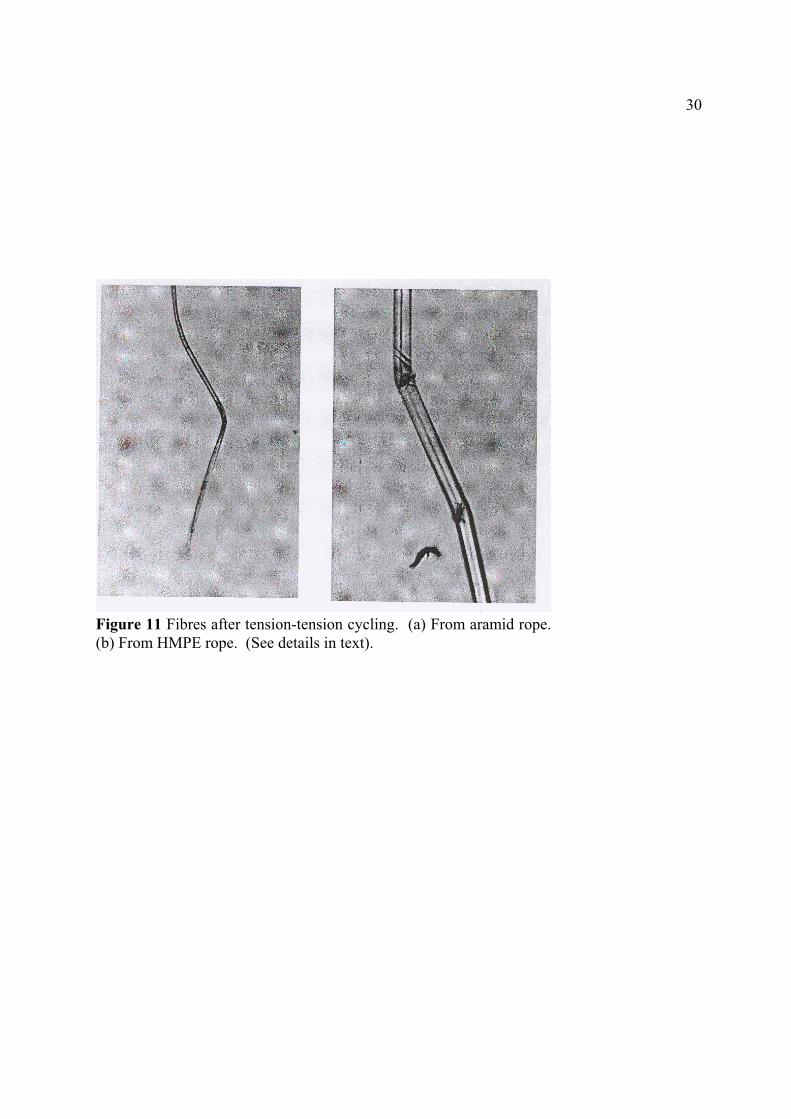
From the UMIST SEM studies, which are reported in greater detail in Hearle et al (1998), Fig.11 (a) shows the appearance of an aramid fibre extracted from the same Twaron rope asspecified above, but cycled at 40+20% break load for one million cycles. Although the ropehad not failed, some yarn breaks had occurred. The appearance at the unbroken end is similarto that shown at the end of the sets of predicted buckle forms in Fig. 6. The next more severebend has broken. Figure 11(b) shows a Twaron fibre from a parallel yarn rope cycled at40+25% break load without failing after one million cycles. The higher magnification showsup the internal kink bands within the fibre at the gross kinks in the fibre as a whole.

A comprehensive and explicit quantitative recording of the buckle parameters was not carriedout in FIBRE TETHERS 2000 (1995). However the above ranges of 3 to 15 mm for the half-wavelength and 35 to 70 mm for the slip length are typical of what was seen. Some of thebuckling appeared to be mode 1, but other examples had up to ten or more buckles in a group. Comparison with the predicted values in Tables IV and V suggest that the yarns tend towardsthe solid rod case, which is not surprising in view of the lateral pressures.

5.0 CONCLUSIONS

The analysis of kinking presented here facilitates a treatment of restrained buckling within

19

ropes and other fibre assemblies. In tension members, axial compression occurs when somecomponents are under axial compressive loading, even though the whole assembly is undertension. In other situations, such as treading on carpets, the loading action may put the wholeof a localised part of the assembly into compression, but within a constrained surrounding ofother yarns. Because oriented fibres have low compressive yield stress, which causes a lowplastic bending moment, the buckling results in sharp kinks, which fail after repeated cycling.

The model, which follows earlier treatments of elastic buckling in pipelines, predicts thatgroups of saw-tooth buckles will be separated by straight slip lengths. The forces involved arethe axial compressive load, the frictional resistance to axial slip, and the lateral restraint ofradial pressure. The yarn modulus and the friction coefficient have a role in determining thedisplacement in the slip zone, which affects the axial compressive force, but the dominantyarn properties are the bending stiffness, which sets the pattern of initial elastic buckling, andthe bending yield moment, which determines the formation of plastic hinges. Unfortunately,there is a wide range of possible values for these quantities, depending on the ease with whichfibres can slide over one another in the yarns. The extremes range from that for the yarnacting as a solid rod to the sum of the bending of the individual fibres. There is alsouncertainty about the numerical values of some controlling parameters and about somefeatures of the model, such as the role of imperfections and the way in which the lateralpressure operates.

While the analysis could be refined, its present accuracy may be close to the accuracy withwhich systems can be defined, and it is debatable where further efforts could best be focussed- on analytic refinements or the acquisition of better data. Nonetheless, the present modeldoes reproduce the experimentally observed pattern of groups of closely spaced kinksseparated by undamaged areas which have unloaded into the adjacent buckle zones. Although the observed values of 3 to 15 mm for the half-wavelength and 35 to 70 mm for theslip length are not entirely within the ranges of 0.25 to 10 mm and 1 to 35 mm respectively forthe predictions in Tables IV and V, the calculated sensitivities are such that it would not bedifficult to find a set of parameters to fit any observed results.

REFERENCES

Allen, S. J., 1987. Tensile recoil measurements of compressive strength for polymeric highperformance fibres, J. Materials Sci. 22, 853-859.

Fibre Tethers 2000, 1995. High Technology Fibres for Deepwater Tethers and Moorings.Noble Denton Europe Ltd, London, England.

Hearle, J.W.S., Lomas, B., and Cooke, W.D., 1998. An Atlas of Fibre Fracture and Damageto Textiles, Woodhead Publishing Company, Cambridge, England.

Hearle, J.W.S., and Miraftab, M., 1991. The Flex Fatigue of Polyamide and Polyester Fibres. Part 1: The Influence of Temperature and Humidity, J. Materials Sci., 26, 2861-2867.

Hearle, J.W.S., and Wong, B.S., 1977. Flexural Fatigue and Surface Abrasion of Kevlar-29and Other High-modulus Fibres, J. Materials Sci. 12, 2447-2455.

Hobbs, R.E., 1984. In-service Buckling of Heated Pipelines, ASCE, J. Transportation

20

Engineering, 110, 175-189.

Hobbs, R.E., and Liang, F., 1989. Thermal Buckling of Pipelines Close to Restraints, 8thInternational Conference on Offshore Mechanics and Arctic Engineering, The Hague, March1989, Vol. 5, pages 121-127.

Riewald, P.G., 1986. Performance Analysis of an Aramid Mooring Line, 18th Annual OTC,Houston, Texas, May 1986, paper OTC 5187.

Riewald, P.G., Walden, R.G., Whitehill, A.S., and Koralek, A.S., 1986. Design andDeployment Parameters Affecting the Survivability of Stranded Aramid Fibre Ropes in theMarine Environment, IEEE OCEANS ‘86, Conference Proceedings, Washington D.C.,September 1986, page 284.

van der Zwaag, S., and Kampschoer, G, 1987. Paper presented at Rolduc Polymer Conference,1987.

Nomenclature

A cross-sectional areac coefficients (Table 2)d element diameterE Young’s moduluse end shortening, “endo”I effective second moment of areak coefficients (Table 1)L buckle half-wavelengthø overall length of buckleLs slip lengthM momentm pd/EIn (P/EI)0.5

N number of fibres in yarnP compressive axial loadp radial pressure on elements inward slip to a bucklex longitudinal coordinatey displacement normal to x

∆ change in quantityµ friction coefficientθ plastic mechanism angle

Subscripts

o original, remote from bucklep plastic

21

s slip^ peakN derivative

Figure 1 Periodic and localised modes

22

Figure 2 Details of lateral buckling

23

Figure 3 Slip lengths and force distribution

24

Figure 4 Geometry of elastic buckles

25

Figure 5 Development of elastic-plastic periodic mode: (a) at elastic limit; (b)incremental plastic mechanism

26

Figure 6 Geometry of plastic localised modes.

27

Figure 7 (a) Elastic buckling in perfect and imperfect situations. (b) Correspondingelasto-plastic buckling

28

Figure 8 Predicted buckling for case specified in text: (a) solid rod; (b) free sliding

29

Figure 9 Core yarn of a core strand in an aramid rope after axialcompression fatigue. (See details in text).

Figure 10 (a)Yarns of outer strand of anHMPE rope after tension-tension cycling. (b)Yarns of core strand. (See details in text).

30

Figure 11 Fibres after tension-tension cycling. (a) From aramid rope.(b) From HMPE rope. (See details in text).