Embed Size (px)
Citation preview

Haar function construction of Brownian bridge and Brownian motion
Wellner; 10/30/2008
Existence of Brownian motion and Brownian bridge as continuousprocesses on C[0, 1]
The aim of this subsection to convince you that both Brownian motionand Brownian bridge exist as continuous Gaussian processes on [0, 1], andthat we can then extend the definition of Brownian motion to [0,∞).Definition 1. Brownian motion (or standard Brownian motion, or a Wienerprocess) S is a Gaussian process with continuous sample functions and:(i) S(0) = 0;(ii) E(S(t)) = 0, 0 ≤ t ≤ 1;(iii) E{S(s)S(t)} = s ∧ t, 0 ≤ s, t ≤ 1.
Definition 2. A Brownian bridge process U is a Gaussian process withcontinuous sample functions and:(i) U(0) = U(1) = 0;(ii) E(U(t)) = 0, 0 ≤ t ≤ 1;(iii) E{U(s)U(t)} = s ∧ t− st, 0 ≤ s, t ≤ 1.
Theorem 1. Brownian motion S and Brownian bridge U exist.
Proof. We first construct a Brownian bridge process U. Let
h00(t) ≡ h(t) ≡
t 0 ≤ t ≤ 1/2 ,1− t 1/2 ≤ t ≤ 1 ,0 elsewhere .
(1)
For n ≥ 1 let
hnj(t) ≡ 2−n/2h(2nt− j), j = 0, . . . , 2n − 1 . (2)
For example, h10(t) = 2−1/2h(2t), h11(t) = 2−1/2h(2t− 1), while
h20(t) = 2−1h(4t), h21(t) = 2−1h(4t− 1) ,
h22(t) = 2−1h(4t− 2), h23(t) = 2−1h(4t− 3) .
Note that |hnj(t)| ≤ 2−n/22−1.The functions {hnj : j = 0, . . . , 2n − 1, n ≥ 0} are called the Schauder
functions; they are integrals of the orthonormal (with respect to Lebesgue
1

measure on [0, 1]) family of functions {gnj : j = 0, . . . , 2n− 1, n ≥ 0} calledthe Haar functions defined by
g00(t) ≡ g(t) ≡ 21[0,1/2](t)− 1,
gnj(t) ≡ 2n/2g00(2nt− j) , j = 0, . . . , 2n − 1, n ≥ 1 .
Thus∫ 1
0
g2nj(t)dt = 1,
∫ 1
0
gnj(t)gn′j′(t)dt = 0 if n 6= n′, or j 6= j′ ,
(3)and
hnj(t) =
∫ t
0
gnj(s)ds, 0 ≤ t ≤ 1 . (4)
Furthermore, the family {gnj}2n−1
j=0, n≥0∪{g(·/2)} is complete: any f ∈ L2(0, 1)has an expansion in terms of the g’s. In fact the Haar basis is the simplestwavelet basis of L2(0, 1), and is the starting point for further developmentsin the area of wavelets.
Now let {Znj}2n−1
j=0, n≥0 be independent identically distributed N(0, 1) ran-dom variables; if we wanted, we could construct all these random variableson the probability space ([0, 1],B[0,1], λ). Define
Vn(t, ω) =2n−1∑j=0
Znj(ω)hnj(t) ,
Um(t, ω) =m∑
n=0
Vn(t, ω) .
For m > k
|Um(t, ω)− Uk(t, ω)| = |m∑
n=k+1
Vn(t, ω)| ≤m∑
n=k+1
|Vn(t, ω)| (5)
where
|Vn(t, ω)| ≤2n−1∑j=0
|Znj(ω)||hnj(t)| ≤ 2−(n/2+1) max0≤j≤2n−1
|Znj(ω)| (6)
since the hnj, j = 0, . . . , 2n − 1 are 6= 0 on disjoint t intervals.
2

Now P (Znj > z) = 1 − Φ(z) ≤ z−1φ(z) for z > 0 (by “Mill’s ratio”) sothat
P (|Znj| ≥ 2√n) = 2P ((Znj ≥ 2
√n) ≤ 2√
2π(2√n)−1e−2n . (7)
Hence
P
(max
0≤j≤2n−1|Znj| ≥ 2
√n
)≤ 2nP (|Z00| ≥ 2
√n) ≤ 2n
√2πn−1/2e−2n ; (8)
since this is a term of a convergent series, by the Borel-Cantelli lemmamax0≤j≤2n−1 |Znj| ≥ 2
√n occurs infinitely often with probability zero; i.e. ex-
cept on a null set, for all ω there is anN = N(ω) such that max0≤j≤2n−1 |Xnj(ω)| <2√n for all n > N(ω). Hence
sup0≤t≤1
|Um(t)− Uk(t)| ≤m∑
n=k+1
2−n/2n1/2 ↓ 0 (9)
for all k,m ≥ N ′ ≥ N(ω). Thus Um(t, ω) converges uniformly as m → ∞with probability one to the (necessarily continuous) function
U(t, ω) ≡∞∑n=0
Vn(t, ω) . (10)
Define U ≡ 0 on the exceptional set. Then U is continuous for all ω.Now {U(t) : 0 ≤ t ≤ 1} is clearly a Gaussian process since it is the sum
of Gaussian processes. We now show that U is in fact a Brownian bridge: byformal calculation (it remains only to justify the interchange of summation
3

and expectation),
E{U(s)U(t)} = E
{∞∑n=0
Vn(s)∞∑
m=0
Vm(t)
}
=∞∑n=0
E{Vn(s)Vn(t)}
=∞∑n=0
E
{2n−1∑j=0
Znj
∫ s
0
gnjdλ
2n−1∑k=0
Znk
∫ t
0
gnkdλ
}
=∞∑n=0
2n−1∑j=0
∫ s
0
gnjdλ
∫ t
0
gnjdλ
=∞∑n=0
2n−1∑j=0
∫ 1
0
1[0,s]gnjdλ
∫ 1
0
1[0,t]gnjdλ+ st− st
=
∫ 1
0
1[0,s](u)1[0,t](u)du− st
= s ∧ t− st
where the next to last equality follows from Parseval’s identity. Thus U isBrownian bridge.
Now let Z be one additional N(0, 1) random variable independent of allthe others used in the construction, and define
S(t) ≡ U(t) + tZ =∞∑n=0
Vn(t) + tZ . (11)
Then S is also Gaussian with 0 mean and
Cov[S(s),S(t)] = Cov[U(s) + sZ,U(t) + tZ]
= Cov[U(s),U(t)] + stV ar(Z)
= s ∧ t− st+ st = s ∧ t .
Thus S is Brownian motion. Since U has continuous sample paths, so doesS. 2
The following figures illustrate the construction given in the theorem.
4
0.2 0.4 0.6 0.8 1.0
0.1
0.2
0.3
0.4
0.5
Figure 1: The Schauder function h00.
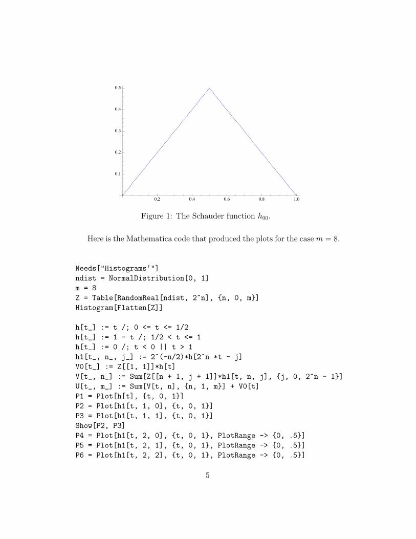
Here is the Mathematica code that produced the plots for the case m = 8.
Needs["Histograms‘"]
ndist = NormalDistribution[0, 1]
m = 8
Z = Table[RandomReal[ndist, 2^n], {n, 0, m}]
Histogram[Flatten[Z]]
h[t_] := t /; 0 <= t <= 1/2
h[t_] := 1 - t /; 1/2 < t <= 1
h[t_] := 0 /; t < 0 || t > 1
h1[t_, n_, j_] := 2^(-n/2)*h[2^n *t - j]
V0[t_] := Z[[1, 1]]*h[t]
V[t_, n_] := Sum[Z[[n + 1, j + 1]]*h1[t, n, j], {j, 0, 2^n - 1}]
U[t_, m_] := Sum[V[t, n], {n, 1, m}] + V0[t]
P1 = Plot[h[t], {t, 0, 1}]
P2 = Plot[h1[t, 1, 0], {t, 0, 1}]
P3 = Plot[h1[t, 1, 1], {t, 0, 1}]
Show[P2, P3]
P4 = Plot[h1[t, 2, 0], {t, 0, 1}, PlotRange -> {0, .5}]
P5 = Plot[h1[t, 2, 1], {t, 0, 1}, PlotRange -> {0, .5}]
P6 = Plot[h1[t, 2, 2], {t, 0, 1}, PlotRange -> {0, .5}]
5

0.2 0.4 0.6 0.8 1.0
0.05
0.10
0.15
0.20
0.25
0.30
0.35
Figure 2: The Schauder functions h10 and h11.
P7 = Plot[h1[t, 2, 3], {t, 0, 1}, PlotRange -> {0, .5}]
Show[P4, P5, P6, P7]
Plot[V0[t], {t, 0, 1}]
Plot[V[t, 1], {t, 0, 1}, PlotStyle -> {Thickness[1/200], RGBColor[0.0, 0.0, 1.00], Dashing[{}]}]
Plot[V[t, 2], {t, 0, 1}, PlotStyle -> {Thickness[1/200], RGBColor[0.1, 0.00, .90], Dashing[{}]}]
Plot[V[t, 3], {t, 0, 1}, PlotStyle -> {Thickness[1/200], RGBColor[0.2, 0.00, .80], Dashing[{}]}]
Plot[V[t, 4], {t, 0, 1}, PlotStyle -> {Thickness[1/200], RGBColor[0.3, 0.00, .70], Dashing[{}]}]
Plot[V[t, 5], {t, 0, 1}, PlotStyle -> {Thickness[1/200], RGBColor[0.4, 0.00, .60], Dashing[{}]}]
Plot[V[t, 6], {t, 0, 1}, PlotStyle -> {Thickness[1/200], RGBColor[0.5, 0.00, .50], Dashing[{}]}]
Plot[V[t, 7], {t, 0, 1}, PlotStyle -> {Thickness[1/200], RGBColor[0.6, 0.00, .40], Dashing[{}]}]
Plot[V[t, 8], {t, 0, 1}, PlotStyle -> {Thickness[1/200], RGBColor[0.7, 0.00, .30], Dashing[{}]}]
Plot[U[t, 8], {t, 0, 1}, PlotStyle -> {Thickness[1/200], RGBColor[0.0, 0.50, .50], Dashing[{}]}]
6

0.0 0.2 0.4 0.6 0.8 1.0
0.1
0.2
0.3
0.4
0.5
Figure 3: The Schauder functions h20, h21, h22, h23.
0.2 0.4 0.6 0.8 1.0
0.05
0.10
0.15
0.20
0.25
Figure 4: A sample path of the random function V0(t).
7

0.2 0.4 0.6 0.8 1.0
!0.10
!0.08
!0.06
!0.04
!0.02
0.02
0.04
Figure 5: A sample path of the random function V1(t).
0.2 0.4 0.6 0.8 1.0
!0.2
!0.1
0.1
0.2
Figure 6: A sample path of the random function V2(t).
8

0.2 0.4 0.6 0.8 1.0
!0.5
!0.4
!0.3
!0.2
!0.1
0.1
Figure 7: A sample path of the random function V3(t).
0.2 0.4 0.6 0.8 1.0
!0.15
!0.10
!0.05
0.05
0.10
0.15
Figure 8: A sample path of the random function V4(t).
9

0.2 0.4 0.6 0.8 1.0
!0.15
!0.10
!0.05
0.05
0.10
0.15
Figure 9: A sample path of the random function V5(t).
0.2 0.4 0.6 0.8 1.0
!0.10
!0.05
0.05
0.10
Figure 10: A sample path of the random function V6(t).
10

0.2 0.4 0.6 0.8 1.0
!0.10
!0.05
0.05
0.10
Figure 11: A sample path of the random function V7(t).
0.2 0.4 0.6 0.8 1.0
!0.04
!0.02
0.02
0.04
Figure 12: A sample path of the random function V8(t).
11

0.2 0.4 0.6 0.8 1.0
-0.4
-0.2
0.2
0.4
0.6
Figure 13: A sample path of the random function U8(t).
0.2 0.4 0.6 0.8 1.0
-0.6
-0.4
-0.2
0.2
0.4
0.6
Figure 14: A sample path of the random function S8(t).
12