Embed Size (px)
Citation preview

Characterisation of Emissions and
Combustion Stability of a Port Fuelled
Spark Ignition Engine
Nicholas M Brown, BSc, MSc.
Thesis submitted to the University of Nottingham for
the degree of Doctor of Philosophy
March 2009
Nicholas M Brown The University of Nottingham
Table of Contents
ABSTRACT............................................................................................................... i
ACKNOWLEDGEMENTS...................................................................................... iii
NOMENCLATURE.................................................................................................. iv
GENERAL SUBSCRIPTS....................................................................................... vi
ABBREVIATIONS................................................................................................. vii
CHAPTER 1 INTRODUCTION................................................... 1
1.1 Background ................................................................................................ 1
1.2 Research Objectives ................................................................................... 3
1.3 Layout of Thesis ........................................................................................ 5
CHAPTER 2 LITERATURE REVIEW ............................................ 8
2.1 Introduction ............................................................................................... 8
2.2 Legislation the European perspective ......................................................... 8
2.3 SI combustion process and factors affecting combustion stability .............. 11
2.3.1 Spark ignition and flame initiation ................................................................. 12
2.3.2 Early flame development ................................................................................ 13
2.3.3 Flame propagation .......................................................................................... 14
2.3.4 Flame termination .......................................................................................... 15
2.4 Measures of cyclic variability .................................................................... 15
2.5 Variable Valve Timing .............................................................................. 17
Nicholas M Brown The University of Nottingham
CHAPTER 3 TEST FACILITY AND KEY EXPERIMENTAL VARIABLES ......... 19
3.1 Introduction .............................................................................................. 19
3.2 Power Plant Description ........................................................................... 19
3.3 Engine control and data acquisition .......................................................... 20
3.4 Test Equipment ........................................................................................ 21
3.5 Determination of Key Experimental Variables .......................................... 22
3.5.1 Determination of relative spark timing .......................................................... 23
3.5.2 AFR calculation and determination ............................................................... 24
3.5.3 Influence of Valve overlap on the residual gas fraction .................................. 27
3.5.4 Comparison of theoretical and measured residual gas fraction ...................... 30
3.5.5 IMEP and COVIMEP ........................................................................................ 35
3.6 Discussion and Summary .......................................................................... 40
CHAPTER 4 DETERMINATION OF MASS FRACTION BURNED ................ 41
4.1 Introduction .............................................................................................. 41
4.2 Rassweiler and Withrow Technique .......................................................... 41
4.2.1 Calculation of the polytropic index for compression ...................................... 44
4.2.2 Calculation of the polytropic index for expansion and methods for
determining the end of combustion ................................................................................ 45
4.2.3 Pressure Referencing ...................................................................................... 46
4.3 Heat release approach ............................................................................... 47
4.3.1 Heat transfer ................................................................................................... 48
4.3.2 Blowby ............................................................................................................ 49
4.3.3 Evaluation of the heat release approach ........................................................ 50
4.4 Discussion and Summary .......................................................................... 52
CHAPTER 5 PHYSICAL AND CHEMICAL LIMITS OF STABLE OPERATION .... 54
5.1 Introduction .............................................................................................. 54

Nicholas M Brown The University of Nottingham
5.2 The influence of chemical and physical parameters on cycle to cycle
stability, initial testing ........................................................................................ 55
5.3 Evaluation of test methodology................................................................. 58
5.3.1 Influence of removing partial burning and misfiring cycles from nIMEPCOV ... 58
5.3.2 Comparison of stability limit from constant air and constant fuel tests
operating at MBT* spark timing ................................................................................... 59
5.3.3 Validity of using net work output to characterise combustion stability ........ 60
5.3.4 Comparison of stability limit from constant air and constant fuel tests
operating at spark timings retarded from MBT* ........................................................... 61
5.4 Comparison of parameters used to define stability limits .......................... 63
5.5 Discussion and Summary .......................................................................... 64
CHAPTER 6 THE CAUSES OF STABILITY LIMITS ............................. 66
6.1 Introduction .............................................................................................. 66
6.2 The change in flame development and rapid burn angle as stability limits
are approached and exceeded at MBT* spark timing .......................................... 67
6.3 The change in flame development and rapid burn angle as stability limits
are approached and exceeded at dMBT* spark timing ........................................ 70
6.4 Discussion and Summary .......................................................................... 72
CHAPTER 7 EMISSONS CHARACTERISATION................................. 74
7.1 Introduction .............................................................................................. 74
7.2 Characterisation of Emissions and Previous Work .................................... 75
7.3 Generic Representation ............................................................................. 76
7.3.1 CO Emissions Index ....................................................................................... 76
7.3.2 HC Emissions Index ....................................................................................... 77
7.3.3 NOx Emissions Index ..................................................................................... 79
7.4 Assessment of emissions models over the NEDC ....................................... 80
Nicholas M Brown The University of Nottingham
7.5 Alternative Approach to Determining MBT* ............................................ 81
7.6 Combustion Efficiency .............................................................................. 82
7.7 Discussion and Summary .......................................................................... 84
CHAPTER 8 EMISSIONS GENERIC FUNCTION PHYSICAL UNDERPINNING .... 86
8.1 Introduction .............................................................................................. 86
8.2 Calculation of cylinder temperature and gas species.................................. 87
8.3 CO Emissions ........................................................................................... 87
8.4 HC Emissions............................................................................................ 90
8.5 NOx Emissions ......................................................................................... 93
8.6 Discussion and Summary .......................................................................... 96
CHAPTER 9 THEORETICAL ASSESSMENT OF STABILITY LIMITS ............. 98
9.1 Introduction .............................................................................................. 98
9.2 Finite heat release model description ........................................................ 98
9.3 Wiebe function investigation ................................................................... 100
9.4 Modelling methodology ........................................................................... 102
9.5 Modelling results ..................................................................................... 103
9.6 Discussion and Summary ........................................................................ 104
CHAPTER 10 DISCUSSION AND CONCLUSIONS............................. 105
10.1 Introduction ............................................................................................ 105
10.2 Discussion ............................................................................................... 105
10.3 Further Work ......................................................................................... 108
Nicholas M Brown The University of Nottingham
10.4 Conclusions ............................................................................................. 109
REFERENCES.......................................................................................................112
TABLES.................................................................................................................120
FIGURES................................................................................................................128

Nicholas M Brown The University of Nottingham
i
Abstract
“Characterisation of Emissions and Combustion
Stability of a Port Fuelled Spark Ignition
Engine”
The chemical and physical limits of cycle-to-cycle combustion variability and engine
out emissions of a gasoline port fuelled spark ignition engine have been investigated.
The experimental investigations were carried out on a V8 engine with port fuel
injection and variable intake valve timing.
The chemical limits of stable combustion have been shown to be a function of
burned gas, fuel and air mixture. The widest limit, gas fuel ratio of <24, burned gas
fraction <0.27 and AFR >9 was found at maximum brake torque spark timing.
Retarding the spark timing by 10oCA caused a small reduction in the stable area,
20oCA retard reduced the stable combustion area significantly, whereby stable
combustion occurred within an area of gas fuel ratio of <19, burned gas fraction
<0.2 and AFR >10.
Burn rate analysis indicated increased variability in both the flame development and
rapid burn period. The increase in variability in the rapid burn period is greater
than that associated with the flame development. The variability is magnified from
flame development through the rapid burn phase. This finding was consistent for
unstable combustion caused by exceeding chemical and physical limits.
Engine out emissions were investigated and characterised using engine global state
parameters, for example AFR, burned gas fraction, for both stable and unstable

Nicholas M Brown The University of Nottingham
ii
combustion conditions. Carbon monoxide and oxides of nitrogen emissions
correlations were unaffected by the presence of unstable combustion events whereas
hydrocarbon emissions showed a significant increase. The incorporation of these
findings were implemented into an engine simulation (Nu-SIM V8) investigating the
impact for the New European Drive Cycle condition.
Nicholas M Brown The University of Nottingham
iii
Acknowledgements
Firstly I would like to thank Professor Paul Shayler, my supervisor at the Engines
Research group. His help, guidance and support throughout the course of
researching and writing this thesis. Thanks is also given to the technical staff of the
Engine Research group, Geoff Fryer and Paul Haywood, for ensuring that the test
facility was kept in top notch working order, and especially John McGhee, for all his
advice and encouragement. All my friends and former colleagues within the
department are also thanked, particularly Adam for helping, advising and
supporting during much of the research.
Thanks also to the Ford Motor Company, the commercial partners of the Engines
Research group, for the provision of the test engine and financial backing.
Finally, I would like to thank my family support and especially my wife, Liz, for all
her help, support, encouragement and, most of all, patience.
Nicholas M Brown The University of Nottingham
iv
Nomenclature
vc Average heat capacity [kJ/kg K]
B Bore [m]
bx Burned gas mass fraction [-]
cr Compression ratio [-]
2R
Correlation coefficient [-]
Crank angle [degs]
sV Cylinder swept volume [m3]
sV Cylinder swept volume [m3]
cyl Cylinder volumetric efficiency [-]
or d Difference [-]
ep Exhaust manifold gas pressure [Pa]
eT Exhaust manifold gas temperature [K]
lossEVO Exhaust valve opening mean effective
pressure loss [kPa or bar]
Q Heat release or transfer [J]
ch Heat transfer coefficient [W/m2K]
lossICW Incremental compression mean effective
pressure loss [kPa or bar]
m Intake manifold gas density [kg/m3]
mp Intake manifold gas pressure [Pa]
mT Intake manifold gas temperature [K]
uS Laminar burning velocity [m/s]
am Mass flow rate of air induced [kg/s]
fm Mass flow rate of fuel induced [kg/s]
fm Mass of fuel in cylinder charge [kg]
mep Mean effective pressure [kPa or bar]
pS Mean piston speed [m/s]
A Measured and calculated oxygen-
containing species to measured carbon [-]

Nicholas M Brown The University of Nottingham
v
containing species
*
ix Mole fraction of species indicated on a dry
basis [-]
ix Mole fraction of species indicated on a wet
basis [-]
ringA Orifice area facilitating cylinder blowby [m2]
n Polytropic index/ Wiebe form factor [-]
p Pressure [bar or Pa]
rx Residual gas mass fraction [-]
R Specific gas constant [J/kg K]
IMEP Standard deviation of indicated mean
effective pressure [kPa or bar]
am Trapped cylinder air mass [kg]
bm Trapped cylinder burned mass [kg]
fm Trapped cylinder fuel mass [kg]
EGRm Trapped external exhaust gas recirculated [kg]
im Trapped intake charge mass [kg]
K Water gas equilibrium constant (3.5) [-]
a Wiebe efficiency factor [-]
cW Work per cycle [J]
Nicholas M Brown The University of Nottingham
vi
General subscripts
0-10% 0-10% mass fraction burned
10-90% 10-90% mass fraction burned
bby Blowby
c Compression
d Delay
e Expansion
f N:C ratio in a given fuel
g Gross
ht Heat transfer
i Internal
id Ignition delay
max Maximum value
n Net
s Spark
y H:C ratio in a given fuel
z O:C ratio in a given fuel
Nicholas M Brown The University of Nottingham
vii
Abbreviations
AFR Air Fuel Ratio
BDC Bottom Dead Centre
CA Crank Angle
CAE Computer Aided Engineering
CCV Cycle to Cycle Variation
CO Carbon Monoxide
CO2 Carbon Dioxide
COV Coefficient of Variance
COVIMEP Coefficient of Variance of IMEP
ECU Engine Control Unit
EDC European Drive Cycle
EGR Exhaust Gas Recirculation
EMS Engine Management System
EOC End of Combustion
EVO Exhaust valve opening
FID Flame Ionisation Detector
FTP75 Federal Test Procedure 75
GDI Gasoline Direct Injection
GFR Gas Fuel Ratio
HC Unburned Hydrocarbon
HCs Unburned Hydrocarbons
HEGO Heated Exhaust Gas Oxygen sensor
IC Internal Combustion
IMEP Indicated Mean Effective Pressure
IMPR Inlet manifold pressure referencing
IVC Intake valve closing
MAF Mass Air Flow
MAP Manifold Absolute Pressure
MBT Maximum Brake Torque
MBT* Minimum Spark Advance for Best Torque
NDIR Nondispersive - Infrared Analysers
NEDC New European Drive Cycle
NO Nitric Oxide
NO2 Nitrogen Dioxide

Nicholas M Brown The University of Nottingham
viii
NOx Oxides of Nitrogen
Nu-SIM Nottingham University Simulation
NVH Noise Vibration and Harshness
O2 Oxygen
OBD Onboard Diagnostics
PFI Port Fuel Injected
PIPR Polytropic index pressure referencing
PMEP Pumping mean effective pressure
PW Pulse Width
rpm Revolutions per minute
SI Spark Ignition
TDC Top Dead Centre
UEGO Universal Exhaust Gas Oxygen sensor
VCT Variable Cam Timing
VO Valve Overlap
VVT Variable Valve Timing
VVTi Variable Intake Valve Timing
WOT Wide Open Throttle
Nicholas M Brown The University of Nottingham
1
CHAPTER 1
Introduction
1.1 Background
This thesis contains two main areas of research both related to gasoline fuelled
spark ignition (SI) engines. Firstly, evaluating the combustion process and causes of
cycle to cycle variability (CCV) and secondly characterising feedgas emissions. The
experimental work was carried out on a modern port fuel injected (PFI) gasoline
engine with variable intake valve timing (VVTi). The application of variable valve
technologies is becoming commonplace amongst the new generation of SI engines,
for reasons which include raising power output, extending the working range of
engine speed and reducing part-load throttling losses. Yet there exists interactions
between valve events and the combustion process that need to be more fully
understood. The aim of the combustion study is to investigate these interactions,
the limits of stable operation and the causes of CCV. Directly linked to this study is
the characterisation of emissions using measurable or easily determinable factors of
engine state and what physics of behaviour underpins the connection of these. The
emissions studies are more generally used to understand engine performance.
The number of cars globally exceeds 550 million with an estimated rate of
production of 45 million cars per year [1]. The market share of diesel powered
passenger cars has increased substantially in Western Europe from 28 to 49% in the
last 6 years [2], in the US the SI engine still remains the power plant of choice with
a significant proportion powered by large capacity V8 engines. The V8 designs are
regarded as having good noise, vibration and harshness (NVH) characteristics
associated with high power at full load, meaning that these engines tend to be
lightly loaded at most in-service operating conditions. The consequence of operating
at light load is that fuel economy and engine-out pollutant emissions are inherently
greater, predominantly due to high throttling losses. Applications of the V8 engine

Nicholas M Brown The University of Nottingham
2
in Europe are mainly found in the luxury vehicle market. Due in part to the higher
profit to cost ratio and customer expectations, electronic throttle control and
variable valve timing first emerge in the same market.
The scope to raise the efficiency of the SI engine through design improvements has
reduced as key parameters such as compression ratio and combustion chamber
design have evolved towards their best achievable values or designs. Modern SI
engines typically have compression ratios between 9 – 11, with pentroof, 4 valve per
cylinder combustion chamber design. These advancements affect the efficiency of the
engine across the entire operating range, yet the diverse nature of the operating
range means there still exists compromises between design variables. Optimisation of
the gas exchange process throughout the operating range by the use of variable
valve timing (VVT) has potential to improve volumetric, mechanical and thermal
efficiencies therefore reducing fuel consumption and emissions. Systems used on
engines vary in complexity that generally fall into two categories variable phase
systems and variable event timing systems, with the ability in either case to add
variable lift.
Application of VVT systems coupled with advances in aftertreatment systems has
increased the interest in the operation of SI engines with lean, dilute mixtures. This
is a potentially more fuel efficient and less polluting mode of operation compared to
traditional SI engines that are required to operate within a close bound around
stoichiometric. One significant problem associated with lean and or dilute mixture
preparation is that the combustion process is likely to be less stable cycle by cycle.
The development of limiting physical and chemical parameters is necessary so
engines can operate in areas that are not associated with increasing cyclic
variability. This can result in a rapid increase in hydrocarbon (HC) emissions and a
noticeable decrease in engine work output.
The move from mechanical to electronic control of the engine has been of significant
importance. Both modern SI and diesel vehicles being controlled by an engine
management system (EMS) embedded in the engine control unit (ECU). The
complexity of the EMS has increased due to more sensors and actuators embedded
in the engine, coupled with increasingly stringent legislation. Particularly important
Nicholas M Brown The University of Nottingham
3
on SI engines is the use of oxygen sensors (commonly known as heated exhaust gas
oxygen sensor (HEGO) and universal heated exhaust gas oxygen sensor (UEGO)).
These sensors are integral in maintaining closed loop fuelling and therefore high
conversion efficiencies of the exhaust aftertreatment system, vital in adhering to
legislation.
The use of computer aided engineering (CAE) has become commonplace in the
automotive industry with models of different complexities being used throughout the
design procedure to reduce development time and optimise the final product. The
drive cycle defined in standard legislative test procedures, the new European drive
cycle (NEDC) in Europe, federal test procedure 75 (FTP75) in North America, for
example are used to simulate operating conditions arising in vehicle service. Driving
vehicles through these standard cycles allows a standardised comparison of emissions
and fuel economy of different vehicles. Development of vehicle models that predict
engine performance over the drive cycle, off cycle and steady state conditions
enables evaluation of important system interactions that effect emissions and fuel
economy. The models can be used in the development stages of the vehicle allowing
evaluation of strategy and calibration changes. Importantly the model can be used
to evaluate the effect of sensor failure or degradation on emissions and the resulting
consequences on the aftertreatment system over the vehicle lifetime, on a legislative
perspective, 80,000km or 5 years (Euro III), from January 2005 (Euro IV)
100,000km or 5 years [3].
1.2 Research Objectives
Specific tasks undertaken include:
Investigate the chemical (air/fuel/residual fractions) and physical (spark
timing) limits of stable work output of a V8 SI engine with VVTi.
Investigate, evaluate and utilise the most robust method for calculating the
mass fraction burned rates from the measured cylinder pressure data.
Nicholas M Brown The University of Nottingham
4
Determine the instability of which part of the combustion event, flame
development or rapid burn causes unstable work output.
Develop a set of emissions generic functions, describing CO, HC and NOx
emissions across the full operating range of the V8 engine.
Incorporate and assess the influence of the emissions generic functions
developed over the NEDC in Nottingham University Simulation (Nu-SIM)
V8
Compare and contrast the generic functions with physical based emissions
models.
The investigations reported in this thesis are primarily concerned with the
combustion process and emissions from a PFI SI engine with VVTi. Previous work
[4] established combustion stability limits based on variability in the work output of
an I4 engine both at fully warm and cold operation. The transition from stable to
unstable operation at a range of engine speeds and loads was characterised using the
mixture gas fuel ratio (GFR). It was found that at fully warm conditions a rapid
decay in combustion stability consistently occurred at a GFR of 25:1. This study
only investigated the variations in work output, no analysis of the combustion was
provided. Further work by Lai [5] used experimental data to develop boundaries of
stable work output based on chemical factors, namely, GFR, burned gas fraction
( bx ) and air fuel ratio (AFR), with minimal investigation on the influence of spark
timing, using similar methodology to that of [4]. Analysis of the combustion was
provided using software developed by the author, where overall, variations in work
output were caused as the burn progresses through the charge with little pre-
conditions from the early stages of flame development. The aim of the current work
was to further investigate the limits on stable operation including a detailed study
of the influence of spark retard, since this is routinely used as a method of reducing
catalyst light off times by increasing the burned gas temperature. The cause of the
variation in work output is investigated by calculating and correlating burn rates
and key burn parameters. Specifically investigating the correlation between
variability in the flame development and rapid burn angle. Additional to this work
is a comparison with alternative methods of defining mixture limits on stable
Nicholas M Brown The University of Nottingham
5
operation that have been applied to PFI gasoline engines operating on a mixture of
liquid and hydrogen fuel [6].
Previous work [7] showed that emissions of carbon monoxide (CO), oxides of
nitrogen (NOx combination of nitric oxide (NO) and nitrogen dioxide(NO2)) and
unburned hydrocarbons (HCs) from three fixed valve timing SI engines were all very
similar and could be represented using ‘generic functions’ based on measured engine
parameters. These functions have been applied to a data set from the V8, with
particular emphasis on the influence of variable valve timing which has not been
previously investigated. The effect of unstable combustion conditions on emissions is
characterised separately. The emissions data is used to calculate combustion
efficiency, highlighting the importance of determining stable operating limits, which
are particularly important when variable valve strategies are available. Finally in
some cases, previously developed physical models are compared with the results
from the ‘generic functions’
The findings from the experimental work have been used to develop feature models
that have been used in a V8 version of Nu-SIM, the initial Nu-SIM V8 was
developed by Harbor [8] for which the author contributed a significant amount of
engine data to which sub models were fitted. These models have been further
reviewed and updated in light of the findings from the combustion and emissions
study, incorporating the combustion efficiency calculations allowing the influence of
unstable combustion cycles to be accurately represented by a representative drop in
work output. Results from Nu-SIM are presented over the NEDC assessing the
effect of the new emissions models.
1.3 Layout of Thesis
The investigations in this thesis include further development of mixture limits on
combustion stability, characterisation of emissions and development and
implementation of feature models in Nu-SIM V8. In Chapter 2, relevant literature is

Nicholas M Brown The University of Nottingham
6
reviewed in relation to the combustion process, included is a historical and current
review of European legislation relating to motor vehicles.
In Chapter 3, a review of the engine test facility is presented. This includes an
overview of the hardware and software used to capture the engine data. Methods
used to calculate key experimental variables are presented. Of key importance the
method and results from the in-cylinder gas sampling system, used to characterise
the influence of variable valve timing on the residual gas fraction.
In Chapter 4, methods of determining mass fraction burned parameters are assessed.
These are the Rassweiler and Withrow method and the traditional first law of
thermodynamics approach. Results from the two methods as the combustion process
becomes unstable are compared. Critically, the number of cycles required to
accurately calculate burned mass fraction values is defined.
In Chapter 5, the chemical and physical limits on combustion stability in terms of a
limit on cyclic variability of indicated mean effective pressure (IMEP) are defined.
The data used was taken from sweeps carried out in three different ways: either
constant fuelling, air charge or load at engine speeds and loads typical of the V8
engine.
Chapter 6 develops the causes of CCV by establishing the link between the
variation of IMEP with burned mass fraction data.
Chapter 7 uses the functional form of the previously developed ‘generic functions’ [7]
to fit the emissions data from the V8 engine. The influence of VVTi is taken into
account by adding new functions; an assessment of an alternative method for
determining relative spark timing and variations in combustion efficiency is also
presented. The influence of the newly developed emissions and combustion models
on vehicle performance are shown by comparing outputs from the V8 version of Nu-
Sim. Chapter 8 reviews literature related to the emissions work developed in
Chapter 7, where applicable the ‘generic functions’ are underpinned using previously
developed physical models. In the case of HC emissions the functions are broken
down into two parts, emissions resulting from normal combustion process and those
from unstable operating conditions.

Nicholas M Brown The University of Nottingham
7
Chapter 9 is used to revisit the stability investigation. A simple heat release model
is used to investigate the relationship between variability in the flame development
and the rapid burn periods, where the variations in heat release was produced by
manipulating the Wiebe function.
Discussions and conclusion are provided in chapter 10.
Nicholas M Brown The University of Nottingham
8
CHAPTER 2
Literature Review
2.1 Introduction
Relevant literature and background to the work presented in this thesis are reviewed
in this chapter, although specific literature relating to emission formation
mechanisms is reviewed in the relevant chapter. Firstly, European legislation
relating to SI motor vehicles are described in detail from its inception to the current
standards, with reference to Onboard Diagnostics (OBD). An overview of the
combustion process is provided, discussing previous work that has described the
causes of cycle to cycle variability. Methods of extending stability limits and
emerging gasoline technology that are capable of utilizing these technologies are also
discussed. VVT strategies are introduced, with both the types and effects of each
system being reviewed.
2.2 Legislation the European perspective
This section focuses on the development of emissions legislation relating to motor
vehicles within the European Community, Figure 1 provides an overview of the
emissions limits imposed and the associated percentage reduction of each emission
from the first legislation. The first legislation came into force in 1970 [9] this
legislation only related to spark ignition engines, imposing limits on emissions of
HCs and CO. The legislation comprised three separate tests. The type 1 test, known
as the European Drive Cycle (EDC) shown in Figure 2 was designed to mimic
conditions of urban journeys from an initial cold engine start. The test lasting
thirteen minutes comprised four cycles that were carried out without interruption,
each cycle containing 15 phases (idling, acceleration, steady speed, deceleration,
Nicholas M Brown The University of Nottingham
9
etc). The vehicle was soaked prior to the test for a period of six hours at between 20
to 30oC, the actual test start, when exhaust gas collection began, was 40 second
after the initial attempt to start the engine. The mass of CO and HCs had to be less
than the legislative limit, where the limits varied with vehicle reference weight as
indicated by the error bars. Conformity of production for a series of vehicles was
also described, where CO and HC limits had to be no greater than 20% and 30%
higher than the legislative limits respectively. Test types 2 and 3 limited CO
emissions at idle and HC crankcase emissions respectively. Emissions of NOx were
not included in the legislation until 19761. The conflicting engine strategies required
to reduce NOx and HC emissions simultaneously was reflected in the legislation
when a further refinement in 19832 combined these two emissions into one limit,
thus allowing engine manufacturers to pursue strategies to lower NOx or HC
emissions. The new legislation also applied to diesel powered vehicles, due essentially
to the increased market share. Although further legislation altered vehicle
categorisation and introduced limits on particulates, significant changes to the
vehicle testing procedure occurred with the introduction of what is commonly
known as Euro I legislation [9]3.
The Euro I legislation altered test type 1 (the EDC) by introducing an extra urban
cycle proceeding the four elementary urban cycles as shown in Figure 2, with the
new drive cycle known as the new EDC (NEDC). The issues of fuel economy were
raised whereby in the future measures to curb carbon dioxide (CO2) emissions would
be proposed. Euro I legislation for spark ignition engines was only achievable with
exhaust after treatment systems; these systems require specific operating conditions
to maintain high conversion efficiencies [10]. The emissions recorded for the type 1
1 Date of legislation, type approval required from 01/10/77, prohibit the entry into service of
vehicles from 1/10/80.
2 Date of legislation, type approval required from 01/10/84, prohibit the entry into service of
vehicles from 1/10/86.
3 Date of legislation, type approval required from 01/7/92, prohibit entry into service of
vehicles from 31/12/92.

Nicholas M Brown The University of Nottingham
10
test were therefore multiplied by a deterioration factor, supplied by the
manufacturer, based on experimental data, or specified in the legislation, the aim
that the aftertreatment system was robust enough to meet the standards for
80,000km. Euro I also introduced limits on evaporative emissions. To increase the
rate of development of cleaner vehicles that would meet new legislation earlier,
provisions for tax incentives were put in place to equal the expenditure on the
aftertreatment costs. Euro II further reduced the emissions limits.
Euro III and IV legislation were introduced together in 19984, with different
implementation dates, allowing engine manufacturers to better plan the engine and
aftertreatment system developments required to meet the future standards and take
full advantage of the tax incentives available if they met the standards early. Along
with the further reduction in the emissions levels significant changes to the vehicle
tests were made. Emissions were sampled from key on for the NEDC and a new test
was introduced to specifically legislate against cold start emissions, namely CO (15
g/km) and HCs (1.8 g/km), where the vehicle was driven over the EDC with the
ambient temperature maintained at -7oC.
The issues of maintaining highly efficient emissions control systems over the vehicle
lifetime were further addressed with the introduction of OBD for emissions control
systems. ‚Emissions control systems‛ were defined as the EMS and any emission-
related component in the exhaust or evaporative system which supplies an input or
receives an output from the EMS. The OBD system must have the capability to
record in the EMS any malfunction of an emission-related component or system that
would result in emissions exceeding the limits. Specifically related to SI engines, it
was necessary to be able to detect and log engine misfire either caused by poor fuel
metering or the absence of spark, if the occurrence of misfire exceeded a certain
threshold then fuelling was disabled to the misfiring cylinder. Oxygen sensors
(HEGO and/or UEGO) needed to be checked for continuity and fuelling
4 Date of legislation, Euro III type approval required from 01/01/00, prohibit entry into
service from 1/01/02, Euro IV type approval from 01/01/05, prohibit entry into service from
01/01/06

Nicholas M Brown The University of Nottingham
11
perturbation strategies needed to be included as part of the EMS to check for failing
catalysts. The OBD test in the legislation required manufacturers to supply faulty
components that needed to flag errors when the vehicle was driven over the NEDC.
The direct impact on the consumer was that the vehicle is fitted with an OBD dash
light, that illuminates when OBD faults are registered, this indicates the EMS has
moved into a limp home or emergency start-up strategy and requires the fault to be
diagnosed and remedied. Finally, the move from Euro III to IV requires the
increased robustness of the emission control system with conformity of in service
vehicles required for 100,000km compared to 80,000km previously.
Significant reductions in vehicle out emissions have been achieved since the
introduction of legislation, although much of the reduction has been achieved with
aftertreatment systems, which necessitates, in SI engines for the combustion system
to be operating at a relatively stable condition, namely stoichiometric. The drive for
lower CO2 emissions both from the customer and governments needs advancements
in the combustion system so as to achieve the minimum fuel consumption. These
necessary changes are likely to move the combustion process towards less stable
regimes, which need to be fully understood before a successful design can be
productionised.
2.3 SI combustion process and factors affecting
combustion stability
In a PFI spark ignition engine in which fuel and air are inducted together, forming a
relatively homogeneous mixture, it is plausible to divide the combustion process of
this mixture into four distinct phases: (1) spark ignition; (2) early flame
development; (3) flame propagation; and (4) flame termination. It is widely accepted
[11,12,13,14] that significant improvements in fuel economy can be achieved by
operating with lean or dilute mixtures. Three factors are predominant in causing the
improvement in fuel economy: (1) reduced pumping work at constant break load
(with dilute mixtures because fuel and air remain constant; hence intake pressure

Nicholas M Brown The University of Nottingham
12
increases, with lean mixtures because the air is increased; hence intake pressure
increases); (2) reduced heat transfer to the walls because the burned gas
temperature is decreased significantly; and (3) a reduction in the degree of
dissociation in the high-temperature burned gases which allows more of the fuel’s
chemical energy to be converted to sensible energy near TDC. The first two of these
are comparable in magnitude and each is about twice as important as the third. The
problem associated with lean and dilute mixtures is that the combustion process is
significantly less robust. The mixture is harder to ignite and flame propagation is
slower with a greater susceptibility for partial burning, a combination of these
factors leads to an unacceptable increase in cyclic variability limiting the range of
operating conditions. The next sections provide a review of each phase of
combustion discussing techniques used to reduce cyclic variability therefore
extending the stable operating range.
2.3.1 Spark ignition and flame initiation
The ignition energy required to ignite quiescent stoichiometric gasoline and air
mixture is about 0.2mJ. Conventional ignition system delivers a spark with 30 to
50mJ where spark durations are greater than 0.5ms [14]. In a typical spark
discharge there are a number of important phases, namely the breakdown, electrical
arc and glow discharge phases. The first two phases establish the ignition plasma; it
is during the glow discharge phase that self sustaining propagation of the flame
kernel begins. The successful development of a flame kernel depends on a large
number of parameters such as ignition energy, plasma volume and location,
chemical reactions, mean flow field and turbulence around the spark plug location
[15]. Even if successful propagation of the flame kernel occurs fluctuations in any of
the factors mentioned contribute to CCV. A number of researchers have
investigated methods of enhancing the flame ignition. A comprehensive study of
different ignition systems by Geiger et al [16] showed that transistorized coil ignition
systems lead to better flame initiation of lean mixtures than a capacity-discharge
ignition system. In the same study, spark plugs with thin electrodes and extended
electrode gaps were found to extend the lean limit for stable combustion which was
Nicholas M Brown The University of Nottingham
13
corroborated by the findings of [17-20]. The study by Rivin et al [19] using a disc-
shape high swirl combustion chamber operating on lean methane mixtures
investigated the spark plug orientation and flow velocity through the spark gap.
Enhanced spark discharge characteristics (80mJ spark energy) were able to achieve
reliable ignition of ultra lean mixtures (equivalence ratios of between 0.62 to 0.64).
The spark plug orientation was found to have no influence on the lean misfire limit.
At high flow velocities past the spark gap (8.6m/s) no reliable combustion of the
mixtures with an equivalence ratio of 0.66 could be achieved, even with the
enhanced spark discharge system. This failure to ignite is likely to be caused by
excessive stretching of the flame kernel [21]. Many engine based studies [22-24]
however, have highlighted that increasing the mean flow velocity and the turbulence
using a variety of different mechanisms extends the lean operating limit by reducing
the onset of excessively high cycle to cycle variations.
2.3.2 Early flame development
The early flame development period is typically defined by the period between spark
and a specified mass fraction burned, although the criteria used varies between
different researchers. Early research by Hires et al [24] referred to the flame
development stage as the initiation stage, or ‘ignition delay’, which was the period
from spark to one percent mass fraction burned. Although this was an arbitrary
point it represented a state where significant energy release began and a fully
developed flame front had been established. This period has been used by other
researchers [25-27] to help understand the causes of cyclic variability and lean
operating limits. Alternatively 2 percent mass fraction period [28] and the 10
percent mass fraction period [22,29] have been used when establishing causes of
cyclic variability. In most cases no reasons are provided as to the choice of period,
the choice simply being arbitrary, others [30] however state that the earliest period
that can be investigated is dependent on the noise in the pressure measurements
and heat release calculations. Because researchers have used various different
periods, establishing how variability in the early flame development period

Nicholas M Brown The University of Nottingham
14
influences the overall combustion process and therefore variability in work output is
hard to ascertain.
Work by Holmstrom and Denbratt [31] presented a limited number of experimental
results where the variability in the 0-2, 0-10, 0-50 and 0-90 percent mass fraction
were provided. The same variability was found in each period, indicating how
variability in the early flame development period is maintained throughout the rest
of the burn. A model was developed specifically investigating the contribution to
cyclic variability of random walk of the flame kernel; 0-1 percent mass fraction
burned period. Comparing with the experimental results showed that the model
predicted only 25 percent of the standard deviation of the combustion duration,
IMEP, maximum pressure and location of maximum pressure. It was suggested that
additional variability observed could be attributed to flow field fluctuations causing
variations in the wrinkling and stretching of the flame kernel during the initial flame
development exacerbated by variations in mixing between the fuel, air and residual
gas.
2.3.3 Flame propagation
In this phase the flame is assumed to be fully turbulent and is when the main
portion of in-cylinder charge is burned, commonly referred to as the rapid burn
period. Again this period is defined differently by researchers due to the different
definitions for the flame development period. In all modern SI engines the spark
plug location is in the centre of the combustion chamber and in the absence of a
directed mean flow the flame propagates spherically out from the spark. The rate of
propagation is strongly dependent on the active flame front area and the physical
and chemical properties embodied in the laminar burning velocity, which is solely a
function of mixture composition, temperature and pressure [32]. The development of
the flame kernel directly influences the active flame front of the propagating flame;
therefore cyclic variability will be manifested in the flame propagation period. The
contribution to overall cyclic variability from only the flame propagation period is
therefore complex to resolve from experimental work.

Nicholas M Brown The University of Nottingham
15
2.3.4 Flame termination
Flame termination is characterised, typically as the period of 90 to 100 percent mass
fraction burned. In this period the flame impinges on the cylinder walls, locally
quenching the flame and significantly slowing the rate of burn. Cyclic variability in
this period is likely to have been manifested by variability in the flame development
and rapid burn period. Comparisons of calculated mass fraction burned profiles and
Schlieren images of the propagating flame indicate that even when essentially 100
percent of the mass has been burned there is still the presence of burning charge
[33].
2.4 Measures of cyclic variability
The most important factor with regard to engine performance characteristics is the
CCV in IMEP, the most commonly used term used to define the variability is the
coefficient of variation ( IMEPCOV ) in IMEP (COV is defined as the standard
deviation divided by the mean). IMEP is related to the in-cylinder pressure history
and is therefore influenced by various factors such as the rate of heat release from
the combustion, heat losses to the cylinder walls and cylinder volume change due to
piston motion. It has been shown [34,14] that IMEPCOV in the order of 10 percent
can result in vehicle driveability problems. Although in the past different thresholds
have been used; 6 percent [35], 7 percent [36], 13 percent [37] and 36 percent [38].
More recent work by Hill [39] suggested the IMEPCOV limit should be set to 5
percent, the limit was set more conservatively than other researchers to allow some
room for overshoot on controllers thus ensuring driveability would not be
compromised. Work using a single cylinder engine [17] looking at methods to extend
the lean misfire limit used IMEPCOV of 2 percent as the threshold value. The limit
used will be dependent on experimental equipment. For example factors such as
engine cylinder number, number of cylinders monitored and data acquisition system
will affect the limit.

Nicholas M Brown The University of Nottingham
16
Researchers have in the past used a number of other factors to identify cyclic
variability. A literature review by Ozdor et al [40] identified parameters that had
been used by researchers. There were four distinct areas. Firstly pressure related
parameters, in cylinder peak pressure ( maxp ), in cylinder peak pressure location
(maxp ), maximum rate of pressure rise ( max( / )dp d ), maximum rate of pressure rise
location ( max( / )dp d ), IMEP of individual cycles and IMEPCOV . Secondly combustion
related parameters, maximum rate of heat release ( max( / )dQ d ), maximum burning
mass rate ( max( / )bdx d ), ignition delay ( id), combustion duration ( d
) and
time in crank angles elapsed from ignition to a moment at which a certain mass
fraction is burnt ( bx ). Fourthly flame front related parameters and fifthly exhaust
gas related parameters, although both these parameters are used to a lesser extent.
One of the easiest parameters to calculate is maxp since no engine position
measurements are required, yet variations in this parameter have been shown [36] to
initially increase as the lean limit was approached, in a similar fashion to IMEPCOV .
Once IMEPCOV exceeded 5 percent variations in maxp were found to actually
decrease. This can be explained by the fact that near the misfire limit the pressure
due to combustion is negligible therefore maxp will simply reflect the compression
pressure which is constant for a given load therefore variability will decrease. This
would also apply, therefore to variability in maxp . A study by Brown et al [12] came
to similar conclusions where IMEPCOV and maxpCOV showed no correlation when the
ignition timing was varied.
The heat release profile is calculated using the first law of thermodynamics which
can also be used to calculate the mass fraction burned profiles, although it is more
usual to calculate burn parameters using the Rassweiler and Withrow method.
Typically the approach adopted by researchers [17], in recent times is to use
IMEPCOV as the key variable to determine cyclic variability and analyse the causes
of the IMEPCOV from calculated burn parameters. These typically include the use of
different burn durations, for example 0-10 percent mass fraction burned (flame
development angle ( 0 10%( ) )) and 10-90 percent (rapid burn angle ( 10 90%( ) )).

Nicholas M Brown The University of Nottingham
17
The variation of researchers’ approaches to investigate CCV makes it difficult to
compare results and establish definitive reasons for the causes of the variability. It is
though necessary to investigate both the variability in work output from the engine,
namely IMEP and to understand the root causes of this variability, analyse the
burn rates, simply investigating pressure related parameters are unlikely to provide
significant information to understand the variations.
2.5 Variable Valve Timing
The manipulation of valve timings provides the ability to overcome some constraints
that are implicit with an SI automotive engine design, since typically a compromise
between valve timings to maintain stable idle combustion and wide open throttle
(WOT) maximum power needs to be adopted [41].
VVT can be used to describe variable phasing mechanisms, where the valves open
and close at different times in the cycle, where on simple systems phasing the intake
valve is preferred, with more complex systems phasing both the intake and exhaust.
Some systems also utilise variable valve lift along with phasing where typically two
or three settings are available, finally the most complex of systems utilise both
intake and exhaust valve phasing and lift where the lift can be different for each
intake or exhaust valves. Many mechanisms have been investigated to implement
VVT. Work by Moriya et al [42] tabulated the merits of many different designs
during the description of the development of a continuously variable intake cam
phasing system, as with many systems the one offering the most independence and
therefore the greatest of possible benefits, electromagnetic controlled valves is also
the most complex and hardest to implement. Although comparing the deliverables
namely, increased power, torque, fuel economy and a reduction in emissions against
the number of additional parts cam phasing was described as being the most cost
effective.
Variable intake cam phasing has been investigated by a number of researchers [43-
45]. Leone et al [43] showed that a significant benefit of advancing the intake valve
Nicholas M Brown The University of Nottingham
18
timing at part load was that the residual gas fraction ( rx ) substantially increased,
this resulted in a direct reduction in NOx and HC emissions, pumping work is also
reduced due to the increased internal residual recirculation therefore a higher
manifold absolute pressure (MAP) is required to maintain a given load. The results
were compared with dual equal and exhaust only valve phasing where dual equal
was found to provide the greatest fuel economy benefit and exhaust only greatest
NOx reduction, concerns were also raised with the intake only strategy since this
increased the probability for engine knock. Duckworth and Barker [44] included port
throttling investigations alongside variable intake cam phasing, benefits were found
from both systems. Specifically from the variable valve phasing improved idle
stability, peak power and fuel consumption was demonstrated; specific reference was
made to the ability to replace external exhaust gas recirculation (EGR) systems
with the internal EGR created by changing the valve timing.

Nicholas M Brown The University of Nottingham
19
CHAPTER 3
Test Facilities and Key Experimental
Variables
3.1 Introduction
This chapter describes the engine test facility, data acquisition system and how key
experimental variables were determined, namely, AFR, burned gas fraction ( bx ),
minimum spark advance for best torque ( *MBT ), IMEP and IMEPCOV . The test
engine was a production Jaguar AJ27; naturally aspirated PFI 4.0l V8. The engine
was equipped with an electronically controlled throttle and variable intake cam
phasing. An in-line automatic transmission was used to couple the engine to a
dynamometer. The engine was instrumented to allow data acquisition while software
provided by Jaguar was used to interrogate and adapt calibration settings of the
EMS. The test facility and software for data acquisition were designed and
implemented by Harbor [8] and Lai [5], and only a brief description is provided here.
The experimental procedure used to determine key variables is described
highlighting the effect of changes in valve overlap (VO) on bx and the particular
problems associated with determining AFR when experimenting at unstable
operating conditions.
3.2 Power Plant Description
The AJ27 is a 90o V8, quad cam, 32 valve engine with an aluminium structure that
has been in production since 1996; Table 1 provides engine specifications as defined
by Szczupak et al [46]. Of particular importance to this study was that the intake
valve timing could be phased over 42oCA, while maintaining a constant opening

Nicholas M Brown The University of Nottingham
20
duration of 230oCA, the exhaust cam timing was fixed, as shown in Figure 3. The
full range of cam phasing was only available above 1000rpm.
The engine was coupled via a production automatic gear box to a 250kW Froude
Consine eddy current dynamometer, the controller of which could run in one of
three modes; constant brake torque, speed or power. The 5 speed gear box was
locked in 4th gear corresponding to a gear ratio of 1:1. Fuel was pumped to the
engine from the original vehicle fuel tank by an external fuel pump, the fuel
supplied was standard pump 95 octane ultra low sulphur unleaded petrol complying
with BS EN 22B; additional specifications are shown in Table 2. A cooling tower
was installed to provide cooling for the engine and dynamometer via different
cooling circuits. An automatic cooling replenishing system was used for directly
cooling the dynamometer, while the engine was cooled indirectly via a heat
exchanger coupled to the engine coolant circuit. An extra heat exchanger was used
to cool the engine oil. The exhaust system was again taken from a production
vehicle and was installed on the test bed with minimal modifications including
catalysts and silencers, allowing representative measurements to be made.
3.3 Engine control and data acquisition
The engine was controlled with a 16bit dual processor production EMS. Calibration
parameters such as spark timing, cam phasing and fuelling could be interrogated
and altered using software provided by Jaguar. The system also allowed 16 EMS
variables to be logged. An independently controlled stepper motor was used to
actuate the pedal position and hence control the electronic throttle.
Data acquisition was achieved using hardware and software (LabVIEW) from
National Instruments. Two data acquisition systems were developed in LabVIEW.
The first, ‘time based’, where steady state measurements such as temperatures, inlet
and exhaust manifold pressures were recorded, the system had the capability to
record from 32 differential analog input channels at typically a rate of 5 Hz. Table 3
shows the variables recorded and relevant location of all the variables logged using
Nicholas M Brown The University of Nottingham
21
the time based data acquisition system. The second ‘triggered based’, was used to
acquire high speed data, primarily for the acquisition of in-cylinder pressure, 8
differential analog input channels could be recorded up a rate of 500kHz, more than
adequate for the range of engine speeds investigated.
3.4 Test Equipment
All thermocouples used were K type with accuracy of ±1oC across the operating
range. Supplementary AFR sensors (Horiba MEXA-700) were installed on both
exhaust lines (one for each bank). The intake and exhaust manifold pressure were
measured using Kulite sensors. Either feed gas or post catalyst emissions could be
sampled using an emissions stack capable of measuring NOx, HC, CO, CO2 and
oxygen (O2). NOx was measured on a wet basis (exhaust gas directly sampled) using
a chemiluminescent gas analyser, HCs were also measured on a wet basis using a
flame ionisation detector (FID) gas analyser, CO and CO2 were measured on a dry
basis using nondispersive - infrared analysers (NDIR) and O2 was measured on a dry
basis using a paramagnetic analyser [47]. All analysers were calibrated following the
manufacturers guidelines before each testing session and recalibrated at the end of
the testing period to check for drift.
In-cylinder pressure was measured in two cylinders, one from each cylinder bank,
with Kistler piezoelectric 6052A high speed pressure transducers flush mounted in
the cylinder head, the signal from the transducer was amplified using Kistler 5011
charge amplifier. The Kistler 6052A is reported [48] to be robust to the intermittent
exposure to the combustion event in an internal combustion (IC) engine which can
result in thermal shock. This is the contraction and expansion of its diaphragm due
to the temperature difference, causing the force applied to the quartz crystal to be
different for a given cylinder pressure. Thermal shock causes errors in pressure
measurements with notable errors in the calculated values of IMEP . The work by
Rai et al [48] has characterised the effect of thermal shock on IMEP using
reference water cooled sensors as a baseline, thermal shock was shown to be
dependent on sensor type, engine speed and peak in-cylinder pressure, with the
Nicholas M Brown The University of Nottingham
22
greatest effects being at low engine speed, high loads and advanced ignition timings.
Results for the Kistler 6052A show IMEP errors due to thermal shock are less than
-1%, with the sensor completely recovering from the effects of thermal shock by the
end of the expansion stroke.
The in-cylinder pressure is logged with reference to the engine crank angle (CA);
CA was measured using a Hohner shaft encoder that was coupled to the crank shaft.
The encoder gave a Top Dead Centre (TDC) pulse and a pulse every 0.5 degrees
crank angle (oCA). Significant errors in calculated values of IMEP can occur when
the cylinder volume is phased incorrectly with the in cylinder pressure, that results
from the cylinder pressure being referenced incorrectly with the crank angle.
Previous work by Brunt [49] has shown that for a 1oCA TDC phasing error, the
associated error in calculated IMEP can be up to 6% for a SI engine operating
from idle to full load. Two methods for determining TDC to accuracies greater than
1oCA are available, analytical determination based on motored traces or a
capacitance probe. Nilsson and Eriksson [50] have analytically investigated 4
methods of determining TDC from simulated pressure traces with the most robust
method determining TDC within 0.1oCA, but the methods are sensitive to errors in
geometry and heat transfer information. The benefit of the capacitance probe is that
it is mounted in the engine and can be used under fired and motored conditions, the
probe outputs a continuous signal based on the proximity of the piston to the probe
and therefore allows direct comparison with the TDC signal from the shaft encoder
as shown in Figure 4. The capacitance probe was successfully used in the engine to
determine TDC to ±0.2oCA, acceptable here since this study focuses on the
variability of IMEP rather than absolute values.
3.5 Determination of Key Experimental Variables
The work presented here relies on the determination and calculation of key
experimental variables. The choice of method used is dependent on the engine
operating condition. The methods are described in the following subsections.
Nicholas M Brown The University of Nottingham
23
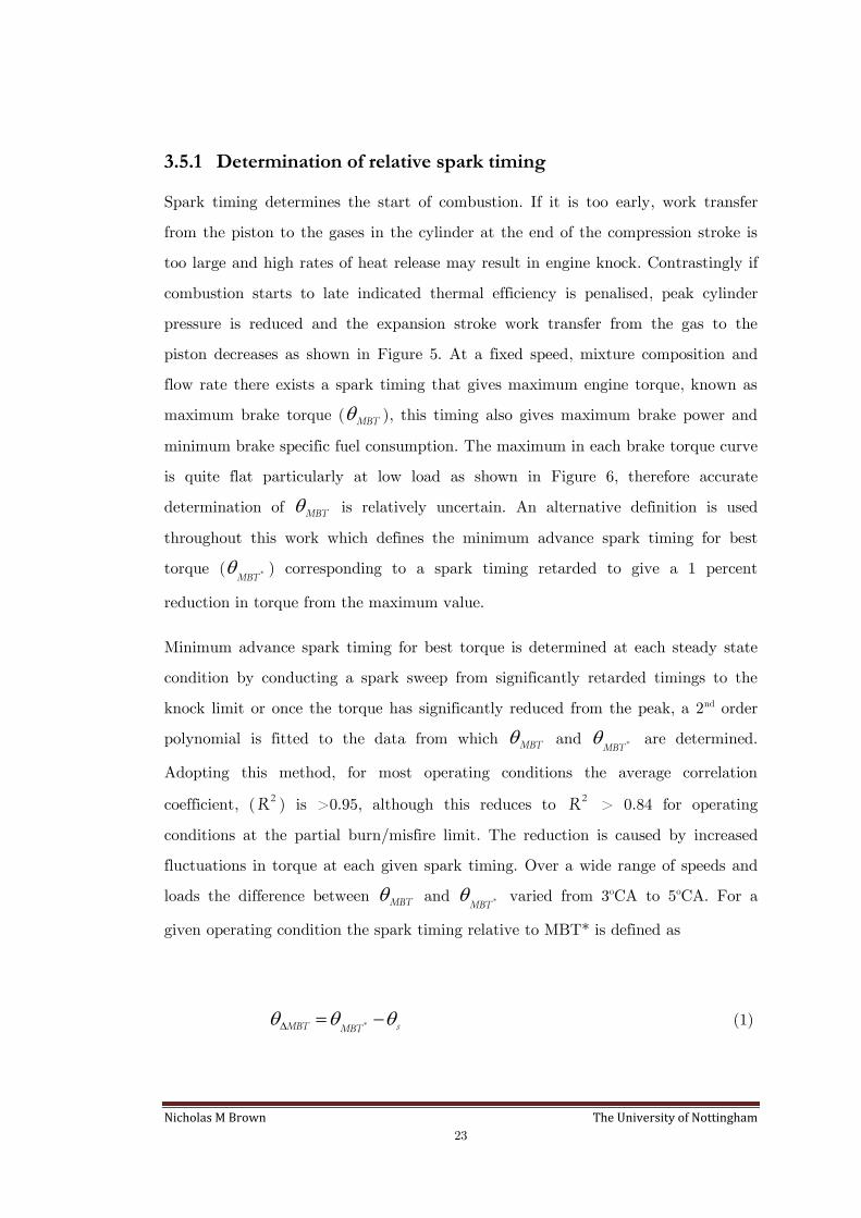
3.5.1 Determination of relative spark timing
Spark timing determines the start of combustion. If it is too early, work transfer
from the piston to the gases in the cylinder at the end of the compression stroke is
too large and high rates of heat release may result in engine knock. Contrastingly if
combustion starts to late indicated thermal efficiency is penalised, peak cylinder
pressure is reduced and the expansion stroke work transfer from the gas to the
piston decreases as shown in Figure 5. At a fixed speed, mixture composition and
flow rate there exists a spark timing that gives maximum engine torque, known as
maximum brake torque ( MBT ), this timing also gives maximum brake power and
minimum brake specific fuel consumption. The maximum in each brake torque curve
is quite flat particularly at low load as shown in Figure 6, therefore accurate
determination of MBT is relatively uncertain. An alternative definition is used
throughout this work which defines the minimum advance spark timing for best
torque ( *MBT ) corresponding to a spark timing retarded to give a 1 percent
reduction in torque from the maximum value.
Minimum advance spark timing for best torque is determined at each steady state
condition by conducting a spark sweep from significantly retarded timings to the
knock limit or once the torque has significantly reduced from the peak, a 2nd order
polynomial is fitted to the data from which MBT and *MBT are determined.
Adopting this method, for most operating conditions the average correlation
coefficient, ( 2R ) is >0.95, although this reduces to 2R > 0.84 for operating
conditions at the partial burn/misfire limit. The reduction is caused by increased
fluctuations in torque at each given spark timing. Over a wide range of speeds and
loads the difference between MBT and *MBT
varied from 3oCA to 5oCA. For a
given operating condition the spark timing relative to MBT* is defined as
*MBT sMBT (1)
Nicholas M Brown The University of Nottingham
24
where s is the absolute spark timing. A value of zero MBT corresponds to MBT*
and a positive MBT refers to spark timings retarded from MBT*.
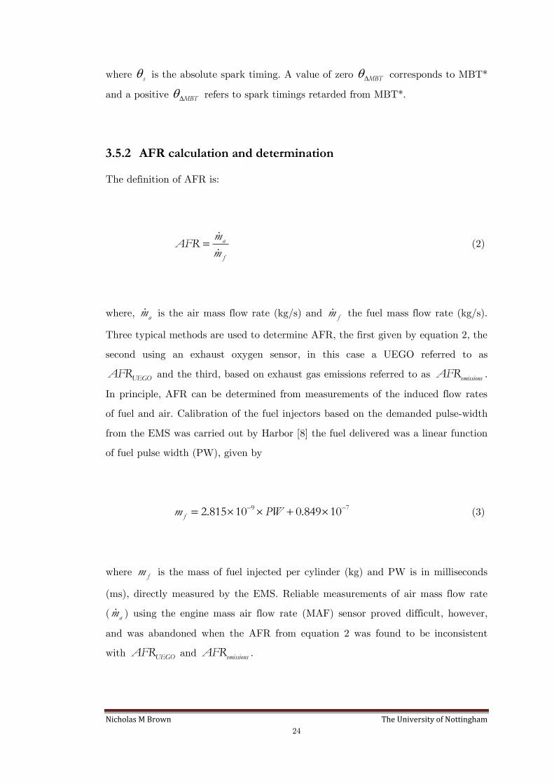
3.5.2 AFR calculation and determination
The definition of AFR is:
a
f
mAFR
m
(2)
where, am is the air mass flow rate (kg/s) and fm the fuel mass flow rate (kg/s).
Three typical methods are used to determine AFR, the first given by equation 2, the
second using an exhaust oxygen sensor, in this case a UEGO referred to as
UEGOAFR and the third, based on exhaust gas emissions referred to as emissionsAFR .
In principle, AFR can be determined from measurements of the induced flow rates
of fuel and air. Calibration of the fuel injectors based on the demanded pulse-width
from the EMS was carried out by Harbor [8] the fuel delivered was a linear function
of fuel pulse width (PW), given by
9 72.815 10 0.849 10fm PW (3)
where fm is the mass of fuel injected per cylinder (kg) and PW is in milliseconds
(ms), directly measured by the EMS. Reliable measurements of air mass flow rate
( am ) using the engine mass air flow rate (MAF) sensor proved difficult, however,
and was abandoned when the AFR from equation 2 was found to be inconsistent
with UEGOAFR and emissionsAFR .
Nicholas M Brown The University of Nottingham
25
Several methods of calculating AFR based on measured exhaust gas emissions have
been proposed [51-54]. An assessment of different methods was carried out by Lynch
and Smith [55], the findings showed that the methods used by Urban and Sharp [54]
and Fukui et al [52] were essentially identical and more accurate than other
methods because fewer simplifying assumptions were made. The method of Urban
and Sharp [54] was therefore applied and is briefly outlined, for a generalised fuel
which can be described as y z fCH O N :
4.773 28.96
12.011 1.008 15.999 14.008emissions
AAFR
y z f
(4)
A is the measured ratio of oxygen-containing species to measured carbon
containing species, y is the H:C ratio assumed to be 1.85, with both z and f
being zero for standard pump grade gasoline. A is given by:
2
2 2 2
2
2
( )( )
2 2 4 4( ) (5)
4 2
CO CO COCO NOCO O NO HC
CO CO
HC CO CO
yx x xx x z yx x x x
Kx xy zA
x x x
K , the water gas equilibrium constant is assumed to be 3.5, with all species, ix
measured as mole fractions with the same background moisture, in this case wet.
The NOx and 2NOx are measured as a combined
xNOx the ratio of 2
:NO NOx x was
set to be constant across all operating conditions as 10:1.
The oxygen concentration was measured using a paramagnetic analyser, the
measured oxygen concentration is affected by other paramagnetic gases, namely

Nicholas M Brown The University of Nottingham
26
NOx , COx and 2COx . A correction to the
2Ox accounting for NOx , COx and 2COx is
made based on values given in [56], where the correct oxygen concentration used in
the emissionsAFR calculation is given by:
2 2 2( ) ( ) 0.442 0.00623 0.00354O corrected O measured NO CO COx x x x x (6)
The exhaust gas emissions are measured directly on a percentage molar volume
basis, 2
*
COx , *
COx and 2
*
Ox are measured on a dry basis whereas HCx and NOx are
measured on a wet basis. The relationship between wet and dry species is given by:
2
*(1 )i H O ix x x (7)
where:
2
2
2 2
* *
* * * *2 [1 /( ) ( /2)( )]
CO CO
H O
CO CO CO CO
x xyx
x Kx y x x
(8)
The Horiba MEXA-700 UEGO sensors are quoted to have an accuracy to within
0.3 AFR in the range of 9.5-20 AFR, and within 2.0 AFR for the rest of the lean
operating range [57]. UEGO sensors all operate on the Nernst principle, basically, by
applying a pump voltage, oxygen from the exhaust gas is pumped through a
diffusion barrier into or out of a diffusion gap that remains at stoichiometric. The
pump current is proportional to the exhaust-gas oxygen concentration and this is a
non-linear measure for AFR [58]. Figure 7 shows the difference in emissionsAFR and
UEGOAFR . For the range shown the difference between emissionsAFR and UHEGOAFR
is within the 10% error, although as indicated by the trendline once the AFR is
greater than 20 the UEGOAFR measures leaner than that determined from the
emissions. This phenomenon is essentially caused by the occurrence of partial and

Nicholas M Brown The University of Nottingham
27
misfiring cycles at those very lean operating conditions, significantly increasing the
HC emissions that results in inaccuracies in measurements from the UEGO and
emissions to different degrees. Winborn [4] highlighted these problems experimenting
at partial burning/misfiring conditions where the UEGOAFR was found to measure
leaner than the mixture ratio supplied. The work involved operating the engine at a
constant throttle angle, engine speed and temperature; it can therefore be assumed
the air charge is constant. The fuel flow rate is therefore directly proportional to
changes in the injector fuel pulse width. Comparing the instantaneous fuel injected
with the fuel injected of a stable AFR at the given operating condition allows
determination of a corrected exhaust gas cAFR during unstable operating
conditions, where:
_
_
emissions stable f stable
c
f unstable condition
AFR mAFR
m (9)
fm
is determined in both cases from equation 3.
Figure 8 compares the inaccuracy
of UEGOAFR and emissionsAFR . It is apparent that UEGOAFR predicts substantially
leaner than the cAFR , although the error associated with using emissionsAFR is less
than the UEGOAFR in the worst case scenario the error difference can be as high as
20%. Based on these findings, at stable operating conditions emissionsAFR was used,
for unstable operating conditions the AFR was calculated from equation 9.
3.5.3 Influence of Valve overlap on the residual gas fraction
VVT is known to affect the in-cylinder residual gas fraction ( rx ). Many researchers
[45, 59-61] have investigated the effect of different VVT mechanisms on the burned
gas fraction, emissions and other engine performance parameters. A comparative
study by Leone et al [43] investigating four variable camshaft timing (VCT)
strategies at part load has described the predominant effects of variable intake cam
phasing. Significant advancement of the intake events extends the VO period into
Nicholas M Brown The University of Nottingham
28
the exhaust stroke, since the intake manifold is at a lower pressure exhaust gas
back-flows from the exhaust port and cylinder into the intake port. This exhaust gas
is then drawn back into the cylinder on the subsequent stroke. Thus increasing the
intake manifold pressure, reducing pumping work and increasing the rx resulting in
a reduction in NOx and HC emissions.
Accurate knowledge of the rx is required for modelling purposes and understanding
combustion and emissions characteristics, for this reason an experimental test
facility was developed to sample in cylinder gases that enabled direct calculation of
the rx . The experimental method and apparatus adopted is similar to that used by
Toda et al [59].
The experimental apparatus and control circuitry was designed and validated
previously [62] although the author aided in adapting the design for application to
the AJ27, therefore a brief summary is given here. A conventional spark plug was
modified to accommodate a 1.2mm capillary tube; this tube was connected to a
E7T05071 Mitsubishi gasoline direct injection (GDI) fuel injector which acted as the
sample valve. Initial design of the apparatus mounted the injector on the engine to
minimise the capillary volume, this design was found to be susceptible to failure due
to high frequency oscillations of the injector, causing the capillary tube to fracture.
A more robust system was implemented where the injector body was mounted away
from the engine but resulted in increased capillary volume hence longer sample
periods.
The sample period was determined indirectly from the ignition timing and once
started was actuated every cycle. The sampling system was designed to ensure that
the injector opened only when in-cylinder pressure was greater than atmospheric.
The end of the sample period was set at 10oCA before sparking, this value was
chosen so as to minimise the effects of the sampling process on combustion. The
sampled in-cylinder gas was directly feed into a CO2 gas analyser. A limiting factor
for the experimental set up was that the CO2 analyser required a minimum flow rate
of 0.3l/min, this was achieved for every test condition by retarding the spark timing
where necessary, hence increasing the sample period and pressure differential.
Operating under these optimised conditions meant there was a time delay of
Nicholas M Brown The University of Nottingham
29
approximately 30s from the start of sampling before the analyser settled to a
constant output representative of the operating condition.
The rx was calculated from the following:
2 2
2 2
c i
e i
CO CO
r
CO CO
x xx
x x
(10)
where the subscripts c, i and e are measured dry in-cylinder, intake manifold and
exhaust CO2 mole fractions, because CO2 mole fractions are measured on a dry
basis. A correction factor Z ,
2
* * *
( ) 1
( ) 1 0.5[ ( ) 0.74 ]
i wet
i dry CO CO CO
xZ
x y x x x
(11)
is used to convert the dry mole fraction measurements to wet.
The sampling period was determined by the spark timing, under light load operating
conditions the spark timing needed to be retarded from MBT* to produce a
sufficient flow rate. Figure 9 shows that changes in relative spark timing have
negligible effects on the measured rx . The effect of VO on the measure rx is shown
in Figure 10a-c. The change in rx is non linear and is only significant for VOs of
greater than 20oCA with the rx more than doubling for a VO change of 42oCA at
1500rpm. The effect of volumetric efficiency is shown by the different load points at
each engine speed, where at higher loads and therefore higher volumetric efficiency
the rx is smaller at all VOs. The rx is influenced by engine speed at a given VO,
reducing engine speed results in increased rx essentially because there is greater
time for exhaust gases to backflow into the cylinder and intake port. The measured
results were used to produce a model of rx using the model based calibration
Nicholas M Brown The University of Nottingham
30
(MBC) toolbox in MATLAB. Engine speed, inlet manifold pressure and VO were
the input factors, contour plots shown in Figure 11, indicate as with the measured
results the highest rx will occur at the lowest engine speed, lightest load and
largest VO. In this case due to the limitations of the cam phasing mechanism the
highest rx of 0.35 was attainable at 1000rpm, 0.44bar inlet manifold pressure and
42oCA VO.
3.5.4 Comparison of theoretical and measured residual gas
fraction
Previous work [4] derived a method to determine the GFR and the rx . This
derivation is shown here. The GFR is defined as the total trapped mass in the
cylinder divided by the trapped fuel mass, which can be expressed in terms of AFR
and the burned gas fraction ( bx ) in the unburned mixture during compression:
bb
a f b
mx
m m m
(12)
where bm is the trapped burned mass, am is the trapped air mass and fm is the
trapped fuel mass, from which
( )
1
a f b
b
b
m m xm
x (13)
The GFR is therefore given by

Nicholas M Brown The University of Nottingham
31
1
1
a f b
f b
m m m AFRGFR
m x
(14)
The burned gas fraction comprises both residual gases from the preceding cycle and
exhaust gas recirculated externally (EGR) which is defined as
EGR
a EGR
mEGR
m m
(15)
The residual gas fraction is defined as
rr
i r
mx
m m
(16)
where the trapped intake charge ( im ) includes the recirculated gas:
i a EGR fm m m m (17)
and
b EGR rm m m (18)
Using equations (14) to (18), the burned gas fraction given by (13) can be expressed
in the form
Nicholas M Brown The University of Nottingham
32
(1 ) .
1
rb r
x AFR EGRx x
AFR EGR (19)
A simple method for estimating the rx was established. Where rx is related to
compression ratio and volumetric efficiency. The use of volumetric efficiency
implicitly accounts for changes in engine speed, throttle angle and the effects of
different intake and exhaust systems. Combining the definition given by equation
(15) and (17),
( )( 1 )a EGR
i
m m AFR EGRm
AFR
(20)
and using volumetric efficiency to define the cylinder volumetric efficiency as based
on the intake mass of normal gaseous components,
a EGR m s cylm m V (21)
where sV is the engine swept volume, cyl
is the volumetric efficiency from
manifold to cylinder and m is the density of the air and recirculated gas mixture in
the intake port, treated as a perfect gas mixture,
( 1 )s cyl m
i
m
V AFR EGR pm
RT AFR (22)
Nicholas M Brown The University of Nottingham
33
where mp is the intake manifold pressure, mT
is the intake manifold temperature
and R is the specific gas constant. If the rx is proportional to the clearance volume
and gas state at the end of the exhaust stroke on the preceding cycle, then
11i e m
c cyl
r m e
m T p AFR EGRY r
m T p AFR (23)
where eT is the exhaust gas temperature, ep is the exhaust gas pressure and cr is
the engine compression ratio, the product of the proportionality constant Y and
the temperature ratio /e mT T are typically close to 2, therefore substituting
equation (23) into equation (16), gives
1
1 2( / )( 1) ( 1 )/r
m e c cyl
xp p r AFR EGR AFR
(24)
Equation (24) has been shown [4] to produce values that are consistent with
literature, in these cases only engines with fixed standard valve timing arrangements
were compared. The error ratio between the measured rx and the predicted rx
(equation 24) is shown in Figure 12. The error ratio in all the cases increases with
larger VOs, the increase being non linear. The error ratio starts to increase from
approximately 10 - 15oCA, with a slight dependence on engine speed. The error ratio
is unaffected by load changes at the three engine speeds since the change in the rx
is accounted for by the volumetric efficiency term in equation (24).
Lai [5] investigated a method of correcting the predicted rx based on equation (19)
by introducing a fictitious ‘internal’ (EGRi) term, where rx was the value predicted
by equation (24) and bx was the measured residual gas fraction. This is equivalent
to the burned gas fraction in this case since the AJ27 had no external EGR system.

Nicholas M Brown The University of Nottingham
34
It was found, to a good approximation that the mass of EGRi was a simple
polynomial function of VO.
7 2 7 5120(2.555 ( ) 7.1105 ( ) 5.1014 )iegrm e VO e VO e
N
(25)
Substituting the value from equation (25) into equation (15)
iegr
i
a iegr
mEGR
m m
(26)
and finally calculating the actual residual gas fraction:
_
(1 ) .
1
r ir corrected r
i
x AFR EGRx x
AFR EGR
(27)
The correlation between the measured and predicted _r correctedx is shown in Figure
13, the empirical trend follows the overall trend from the measured results, with
particularly good performance at the highest measured rx . Although an attempt
was made to apply a semi-physical model described by [63] it was found that this
model under predicted the rx at high VOs. Throughout this work, values for the
rx are calculated from equation 27 ( _r correctedx ).

Nicholas M Brown The University of Nottingham
35
3.5.5 IMEP and COVIMEP
The in-cylinder pressure data can be used to calculate the work transfer from the
gas to the piston per cycle per unit swept volume:
c
s
Wmep
V (28)
where cW is the work delivered per cycle and sV is the swept volume of one
cylinder. For this work, the engine output is measured in terms of the IMEP. There
are two definitions of IMEP, firstly net IMEP ( nIMEP ) which includes all four
strokes
720
0
1n
s
IMEP pdVV
(29)
and gross IMEP ( gIMEP ) which includes only the compression and expansion
strokes
540
180
1n
s
IMEP pdVV
(30)
The difference between nIMEP and gIMEP is termed the pumping mean effective
pressure (PMEP):
n gPMEP IMEP IMEP (31)

Nicholas M Brown The University of Nottingham
36
In the case of the AJ27 the intake cam can be phased, for a conventional engine
with fixed intake cam timing, intake valve closing (IVC) is a trade-off between low
speed torque and high speed power [64]. Phasing the intake cam is in part used to
decrease PMEP, where advancing the intake cam at part load increases the VO and
as has been shown the rx , therefore a higher MAP is required to maintain the load.
The convention described by equations (29) and (30) assumes that the work
associated with exchanging the exhaust gas with fresh charge occurs only during the
exhaust and intake strokes with no impact on the indicated work. Previous work
[65] showed that this method did not allow a valid comparison of the PMEP work
reducing strategies since the convention did not take into account valve timing
effects occurring during the expansion and compression stroke. The method is
described and applied here to clarify the effect of the intake cam phasing on the
work output from the AJ27.
Firstly a calculation is made to account for the expansion work loss by opening the
exhaust valve before bottom dead centre (BDC). This is achieved by extrapolating
the expansion pressure from exhaust valve opening (EVO) to BDC using a curve
fitted to enPV where en is based on the measured expansion stroke data prior to
EVO. The difference between the two areas from EVO to BDC is normalised by the
swept volume as is termed the EVO expansion loss ( lossEVO ),
1
( )BDC
loss extrapolated measured
s EVO
EVO p p dVV
(32)
A similar correction is made for the effects of early or late IVC. With early IVC, the
intake MAP must increase to maintain the same torque. Late IVC allows nearly the
complete elimination of the intake stroke pumping work but results in a large
increase of work during the first part of the compression stroke. This increased work
is termed incremental compression work ( lossICW ) and is quantified in a similar way
to the method adopted to determine the lossEVO . The compression stroke pressure
is extrapolated to BDC based on cnpV with cn determined over an interval where
Nicholas M Brown The University of Nottingham
37
cnpV is approximately linear. The difference between the two areas from BDC to
IVC is normalised by the swept volume and is termed the lossICW :
1
( )IVC
loss extrapolated measured
s BDC
ICW p p dVV
(33)
The work related to the gas exchange process is therefore defined as:
adj loss lossPMEP PMEP ICW EVO (34)
and the adjusted gIMEP is given by:
_g adj g loss lossIMEP IMEP ICW EVO (35)
in both cases lossICW and lossEVO are expressed as positive numbers. Finally the
adjusted _n adjIMEP is given by:
_ _n adj g adj adjIMEP IMEP PMEP (36)
Both cn and en should be close to a value of 1.3. The calculation in both cases is
based on a linear fit to the measured data over 10oCA before spark timing for cn
and 10oCA after the end of combustion for en . The resulting range of cn and en by
applying this method was 1.3±0.04 and 1.3±0.03 respectively. An example of the
extrapolated data is shown in Figure 14 with the intake cam fully retarded (late
Nicholas M Brown The University of Nottingham
38
IVC). The method was applied to a set of data comprising both fully advanced and
retarded IVC timings at two loads and three engine speeds. The torque was held
constant for both valve timings. The effect of the change in the IVC timing on
calculated lossEVO and lossICW is shown in Figure 15 at each engine speed and
load. The change in the calculated lossEVO for the two valve timings is minimal
compared to the change in lossICW , which is a result of the fixed EVO. The
difference between gIMEP and _g adjIMEP is shown in Figure 16, with Figure 17
showing the difference between PMEP and adjPMEP . In both cases the effect of
including lossEVO and lossICW on the PMEP and gIMEP calculations is
insignificant when compared to the traditional integral method. In light of these
results all calculations of work related parameters ( nIMEP , gIMEP and PMEP) are
made using the conventional integral method.
A significant amount of work presented in later chapters focuses on combustion
stability and although many parameters exist to quantify combustion stability,
IMEPCOV is often used since this provides a direct correlation between variability in
combustion and deterioration in vehicle driveability [14, 34]. The definition is given
by:
( )
IMEPIMEPCOV
mean IMEP
(37)
Being that the calculation involves average and standard deviation values,
IMEPCOV will be dependent on the sample size. The required sample size for a
representative value of IMEPCOV was investigated for both stable and unstable
operating conditions. Figure 18 shows the effect of cycle number on the calculated
value of nIMEPCOV for stable operating conditions, after 100 samples the
nIMEPCOV
can be regarded as being representative of the operating condition with any increase
in sample size, up to 1000 cycles resulting in a change in nIMEPCOV of less than
0.1. These findings are similar to those of Hill [39] where for operating conditions

Nicholas M Brown The University of Nottingham
39
where IMEPCOV was less than 5, sample sizes as low as 10 or 20 could give a good
estimation of IMEPCOV . The influence of cycle number during unstable operating
conditions is shown in Figure 19, in this case it is necessary to use a sample size of
500 to gain a representative value of nIMEPCOV , the use of 1000 cycles results in a
change in nIMEPCOV of less than 0.2. This sample size is less than that adopted by
Shayler et al [66] where a sample size of 2000 was used, although the effect of
sample size was not investigated on the value of IMEPCOV . More recent work [6]
investigating stability limits used 400 cycles to calculate IMEPCOV . An evaluation
of IMEP calculation routines and analysis errors by Brunt and Emtage [49]
suggested that the minimum number of cycles to gain a representative mean IMEP
value was 150, it was suggested for best practice that 300 should be used. Although
it is apparent that variable sample sizes could be used to calculate an accurate
IMEPCOV , dependent on operating condition, throughout this work a sample size of
500 is used.
Nicholas M Brown The University of Nottingham
40
3.6 Discussion and Summary
The test facilities have been described. The features of the AJ27 engine used in the
experimental elements of the research have been introduced. A PC-based data
acquisition system was used in conjunction with a Jaguar EMS and software used to
interrogate and manipulate engine variables. The additional engine instrumentation
has been described enabling detailed measurements of the engine condition. A
description of the methodology adopted to determine key experimental variables is
described. These include the determination of maximum brake torque and minimum
advance for best torque spark timing, where a simple 2nd order polynomial was
found to represent the spark sweep accurately. An evaluation of different methods
to determine AFR was carried out, both UEGO and emissions provide similar AFR
measurements at stable operating conditions. At unstable operating conditions
where partial burning/misfiring cycles are apparent, both the AFR calculated from
the emissions and UEGO measure leaner than the actual supplied AFR. Previously
developed experimental apparatus [62] was modified and successfully applied to the
AJ27 to enable the measurement of in-cylinder residual gases ( rx ). Increasing the
valve overlap (VO) by advancing the intake valve opening substantially increases
the rx , although modelled results show that MAP is the most important variable in
determining the rx followed by VO and then rpm. Calculated values of rx were
found to under predict measured rx , an empirical correction factor is applied
allowing reasonable determination of rx across the fully operating range. The
traditional integral method for the calculation of mep was compared to an
alternative method [65] for the full range of VO on the AJ27. The difference
between the calculated values of the two methods was very small; the traditional
method was therefore adopted throughout. Finally it was shown that IMEPCOV is
influenced by sample size, for accurate representation of IMEPCOV over the entire
operating range 500 samples are required.

Nicholas M Brown The University of Nottingham
41
CHAPTER 4
Determination of Mass Fraction Burned
4.1 Introduction
In this chapter, two methods of determining the mass fraction burn profiles are
investigated. The merits of both approaches are examined and important
considerations to be taken into account when applying either method are reviewed.
In both cases the burned mass fraction is determined from the measured in-cylinder
pressure and volume. There are two methods widely used for determining the mass
fraction burn profile. Firstly the Rassweiler and Withrow method, secondly, the
approach based on the first law of thermodynamics, which is applied to both SI and
diesel engines. The main aim of the investigation is to apply both methods, evaluate
the results and decide upon which method will be used throughout this work to
determine the mass fraction burn profiles and related burn duration angles.
4.2 Rassweiler and Withrow Technique
The Rassweiler and Withrow method [67] is based on experimental observations of
combustion in a constant volume bomb. It was found that the mass fraction burned
was approximately equal to the fractional pressure rise.
x x
t t
m pX
m p (38)

Nicholas M Brown The University of Nottingham
42
where m is mass, p is pressure and the suffix t indicates the conditions at the end
of combustion (EOC). For a given amount of energy release in a specific volume, the
combustion pressure rise cp is inversely proportional to the volume V
1cp
V (39)
During combustion in an engine cylinder the pressure change is a result of two
separate processes, pressure change due to combustion and the pressure change due
to piston motion causing a change in volume, V . The compression and expansion
process before and after combustion were found to be well fitted by a polytropic
relation:
constantnpV (40)
Therefore the pressure produced due to V is given by:
n
p
Vp p
V
(41)
where pp is the pressure produced by the change in volume at a given crank angle
( ), p is the pressure measured at the previous half crank position, n is the
polytropic index. The pressure resulting from combustion is therefore given by
c pp p p (42)

Nicholas M Brown The University of Nottingham
43
The calculation of the pressure rise due to combustion can take place at all crank
angle intervals from spark timing to exhaust valve opening. The calculated
combustion pressures have been evaluated at different volumes, to maintain
consistency with the constant volume experiments the pressure must be referenced
to a specific volume, in this case the volume at top dead centre (TDC).
' ( )c p
TDC
Vp p p
V
(43)
The burned mass fraction at any given is therefore,
'
'
cspark
EOC
cspark
p
x
p
(44)
Apart from the required pressure and volume data, a value for the polytropic index
(n ) and end of combustion (EOC) are required. The gas temperature inside the
cylinder during the compression and expansion is different. During compression the
fuel-air mixture and wall temperatures are similar therefore heat flow can occur in
either direction. The compression n will be near to a value of 1.3. Contrastingly the
expansion process, where the gas temperature is significantly higher due to
combustion, results in positive heat flow and normally the calculated expansion
index is lower, although still remains 1.3 (±0.05) [14]. This necessitates the
calculation of individual compression and expansion polytropic indexes.
Nicholas M Brown The University of Nottingham
44
4.2.1 Calculation of the polytropic index for compression
Both polytropic indexes need to be calculated in regions of the pressure data that
are free from combustion, the compression index ( )cn is therefore determined before
spark discharge. The cn is used in the calculation until TDC from then until the
EOC the expansion index e( )n is used. The method used to determine both the
compression and expansion index is outlined in [68]. The n value is established on
the basis of satisfying zero combustion pressure ( ). This uses the relationship
between the n and the predicted over a small crank angle interval. A value of n
is chosen to give equal to zero before combustion commences (spark discharge).
The relationship between n and is approximately linear, as given by:
'{ln( / ) /( ( / ))}
ln( / )
p p p V Vn
V V (45)
Therefore in each case n is identified by linearly interpolation over a range of trial
values until the value of n is found that gives zero . As increases, the value of
n decreases for a compression process and increases for an expansion process.
Due to the effect of signal noise on real data the value of will fluctuate with
crank location. The number of points depends on the signal to noise level of the
combustion pressure record. Previous work [68] calculated the average over a
summation of 10 points at a resolution of 1oCA to suppress the effects of signal
noise. This method was applied here. It was found that the calculated value of the
cn was dependent on spark timing as shown in Figure 20, where the index increases
to values greater than 1.3 for spark timings within 10oCA of top dead centre (TDC),
suggesting strong heat rejection from the gases to the cylinder walls. The influence
of the high cn index on key calculated mass fraction burned angles namely the flame
development angle 0 10%( ) and the rapid burn angle 10 90%( ) is shown in
Figure 21 and Figure 22 respectively. The calculated values are insensitive to
changes in the cn . This is attributed to the cn only being used until TDC.
Nicholas M Brown The University of Nottingham
45
4.2.2 Calculation of the polytropic index for expansion and
methods for determining the end of combustion
The calculation of the en is more complex. In certain cases, the EOC and therefore
the point at which the en is calculated, is determined from the calculated
combustion pressure which is a function of the en . Two of these methods [68] are,
the ‘first negative index’ where the EOC is located when the first negative
combustion pressure occurs. Secondly ‘sum negative index’ where the EOC is
determined when 3 consecutive negative combustion pressures occur. The second
method is seen as a more robust method for determining the EOC since it reduces
the influence of signal noise. In both cases an iterative method is adopted whereby
an initial EOC point is set as 10oCA before exhaust valve opening (EVO). The en is
then calculated using the standard method. A new EOC is then determined using
either method 1 or 2 along with a new en . The loop is exited once there is no
change in the EOC location. Alternatively two different methods adopted by [68]
‘tuned index’ and [69] 1.15' index'pV do not require such an iterative process. For
the tuned index equation 45 is applied to point in the expansion stroke where under
normally combusting cycles combustion will have ceased. The point selected was
just before EVO. The final method 1.15 indexpV simply uses the point where
1.15pV reaches a maximum plus 10oCA to indicate the EOC. In all cases, as with
the cn the en is an average value calculated over 10oCA.
The distribution of the en calculated using the four methods is shown in Figure 23.
The en should be approximately 1.3; therefore the distribution is produced by
normalising the calculated en to 1.3. Both the first negative and the sum negative
methods produce distributions that are biased towards higher values. This is more
noticeable with the sum negative method than with the first negative method, where
the average en is 1.52 and 1.45 respectively. The distribution produced by the
1.15pV method is a very narrow band around the 1.3 value, which is a result of the
method, where the average en is 1.29. The late polytropic index method produces a
distribution that is significantly biased towards higher values of the en this is due
to the relative lateness, compared to the other methods for determining the en . The
Nicholas M Brown The University of Nottingham
46
average en in this case is 1.58. The overall trend exhibited is that the en varies
significantly with the point in the expansion stroke where it is calculated, with
calculations late in the expansion stroke resulting in higher values of the en .
The sensitivity of the 0 10% and the 10 90% to the variation of the en from the
four methods is investigated in Figure 24 and Figure 25 respectively. For
convenience, as with the cn variations in the burn parameters are compared to
those calculated using a fixed, en of 1.3. The mass fraction burn parameters,
particularly the 10 90% are more sensitive to differences in the en than the cn .
The tuned index method for determining the en shows the greatest deviation from
the fixed value, the effect is that the 10 90% in some cases is over twice as long.
This is due to the fact that larger en values suggest heat addition from the gases
resulting in extended burn durations. The difference between all four methods
reduces as the burn duration increases since the EOC point for all four methods
converge to the same point. The 1.15pV method is shown to be the most robust
method for determining the EOC due to the resulting en being close to 1.3.
Throughout this work the mass fraction burned profile is determined using 1.15pV
to locate the EOC.
4.2.3 Pressure Referencing
The in-cylinder pressure measurements are made using piezoelectric transducers.
The piezoelectric transducers measure dynamic pressure rather than absolute and
need to be referenced. It has been shown [70] that incorrect pressure referencing
results in errors of pressure derived parameters such as the polytropic index. Two
methods were investigated, inlet manifold pressure referencing (IMPR) and
polytropic index pressure referencing (PIPR). The disadvantage of PIPR is that a
polytropic index has to be specified and as has been shown the value varies with
operating condition.
The dynamic pressure has therefore been referenced to absolute using IMPR. The
pressure referencing is normally carried out at BDC during induction, taking the

Nicholas M Brown The University of Nottingham
47
average of several points to reduce the sensitivity to noise, typically 10o to 20o CA.
It was found [70] that the correction value was dependent on crank angle and was
suggested this would be engine dependent. This method was applied to measured
data to minimise the inaccuracies associated with incorrect pressure referencing. The
effect of changing the crank angle location of the pressure referencing is shown in
Figure 26. The dynamic pressure averaged over 20oCA ( 10o CA either side of the
reference point) are referenced to inlet manifold pressure, the datum point on the
figure indicating referencing at BDC. Changing the position of the referencing has
an insignificant effect on the absolute pressure, with a change in referencing point of
±15oCA resulting in a change in absolute pressure of ±0.01bar. Pressure referencing
was therefore carried out at BDC.
4.3 Heat release approach
The heat release approach is a single zone model based on the first law of
thermodynamics, where net heat release is given by [14]:
1
1 1
netdQ dV dpp V
d d d
(46)
where p and V are the instantaneous pressure and volume measurements and the
value of gamma ( ) is calculated based on the mixture composition and
temperature at each crank angle using equations developed by NASA [71]. The gross
rate of heat release is calculated by adding the energy exchange to heat transfer and
to blowby to the net rate of heat release as shown by:
1
1 1
gross bbyhtdQ dQdV dp dQ
p Vd d d d d
(47)
Nicholas M Brown The University of Nottingham
48
Integration of the gross heat release from the start to the EOC should give the total
heat released by combustion, where this value under normally combusting
conditions should account for approximately 92 to 96% of the energy supplied in the
fuel. The remainder is attributed to combustion inefficiency, fuel lost in the crevices,
quench layers on the cylinder walls and fuel absorbed into the oil layers on the
cylinder liner and any deposits [72]. The instantaneous heat release divided by the
total provides the mass fraction burned profile from which both the 0 10% and
10 90% are determined.
4.3.1 Heat transfer
Heat transfer on average accounts for between 15 to 20% of the total energy release
[14]. Convective heat transfer is responsible for the majority of the losses.
Convective heat transfer is given by:
ht cQ h A T (48)
where ch is heat transfer coefficient, A is the cylinder surface area and T is the
difference in temperature between the cylinder charge and the cylinder wall ( wT ).
Calculation of the heat transfer coefficient is complex and many uncertainties exist.
The Woschni [73] correlation is used here,
0.2 0.8 0.55 0.83.26ch B p T w (49)
where the units are ch (W/m2K), bore ( )B m , pressure ( )p kPa , temperature
(K)T and velocity ( / )w m s . The average cylinder velocity is determined from
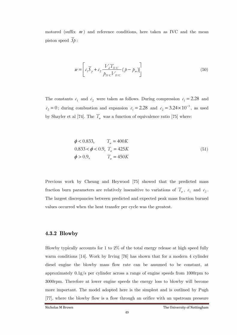
Nicholas M Brown The University of Nottingham
49
motored (suffix m ) and reference conditions, here taken as IVC and the mean
piston speed Sp :
1 2 ( )d IVCp m
IVC IVC
V Tw c S c p p
p V
(50)
The constants 1c and 2c were taken as follows. During compression 1 2.28c and
2 0c ; during combustion and expansion 1 2.28c and 3
2 3.24 10c , as used
by Shayler et al [74]. The wT was a function of equivalence ratio [75] where:
0.833, 400
0.833 0.9, 425
0.9, 450
w
w
w
T K
T K
T K
(51)
Previous work by Cheung and Heywood [75] showed that the predicted mass
fraction burn parameters are relatively insensitive to variations of wT , 1c and 2c .
The largest discrepancies between predicted and expected peak mass fraction burned
values occurred when the heat transfer per cycle was the greatest.
4.3.2 Blowby
Blowby typically accounts for 1 to 2% of the total energy release at high speed fully
warm conditions [14]. Work by Irving [76] has shown that for a modern 4 cylinder
diesel engine the blowby mass flow rate can be assumed to be constant, at
approximately 0.1g/s per cylinder across a range of engine speeds from 1000rpm to
3000rpm. Therefore at lower engine speeds the energy loss to blowby will become
more important. The model adopted here is the simplest and is outlined by Pugh
[77], where the blowby flow is a flow through an orifice with an upstream pressure

Nicholas M Brown The University of Nottingham
50
equal to the cylinder pressure and a downstream pressure equal to crankcase
pressure. This results in choked flow during the compression and expansion stroke of
the cycle. Applying classical one-dimensional isentropic flow and assuming 1.4
the blowby mass flow rate is given by:
1
20.68 ( )bby ringm A p (52)
where ringA is the orifice area, in the absence of experimental data ringA was fitted
so that bbym was a constant value of 0.1g/s at each operating condition. Applying
this method it was found ringA could be set as a constant of 2.71e-7m2. The density
of the cylinder charge is evaluated using the cylinder wall temperature and
measured in-cylinder pressure. The rate of energy transfer to blowby can therefore
be calculated using:
60 1
360 1
bby bby
trapped
dQ m pV
d N m
(53)
where N is the engine speed and trappedm is the total trapped mass of air calculated
from measured air and fuel mass flow rates and the modelled residual mass fraction
given in Chapter 3.
4.3.3 Evaluation of the heat release approach
A set of experimental data was analysed using the heat release approach described
above to investigate the robustness of the models used. Figure 27 shows the
influence of relative spark timing on the percentage of fuel accounted for at three
typical engine speeds. Examination of the proportion of fuel energy released which is
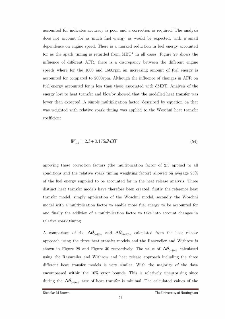
Nicholas M Brown The University of Nottingham
51
accounted for indicates accuracy is poor and a correction is required. The analysis
does not account for as much fuel energy as would be expected, with a small
dependence on engine speed. There is a marked reduction in fuel energy accounted
for as the spark timing is retarded from MBT* in all cases. Figure 28 shows the
influence of different AFR, there is a discrepancy between the different engine
speeds where for the 1000 and 1500rpm an increasing amount of fuel energy is
accounted for compared to 2000rpm. Although the influence of changes in AFR on
fuel energy accounted for is less than those associated with dMBT. Analysis of the
energy lost to heat transfer and blowby showed that the modelled heat transfer was
lower than expected. A simple multiplication factor, described by equation 54 that
was weighted with relative spark timing was applied to the Woschni heat transfer
coefficient
2.3 0.175scaleW dMBT (54)
applying these correction factors (the multiplication factor of 2.3 applied to all
conditions and the relative spark timing weighting factor) allowed on average 95%
of the fuel energy supplied to be accounted for in the heat release analysis. Three
distinct heat transfer models have therefore been created, firstly the reference heat
transfer model, simply application of the Woschni model, secondly the Woschni
model with a multiplication factor to enable more fuel energy to be accounted for
and finally the addition of a multiplication factor to take into account changes in
relative spark timing.
A comparison of the 0 10% and 10 90% calculated from the heat release
approach using the three heat transfer models and the Rassweiler and Withrow is
shown in Figure 29 and Figure 30 respectively. The value of 0 10% calculated
using the Rassweiler and Withrow and heat release approach including the three
different heat transfer models is very similar. With the majority of the data
encompassed within the 10% error bounds. This is relatively unsurprising since
during the 0 10% rate of heat transfer is minimal. The calculated values of the
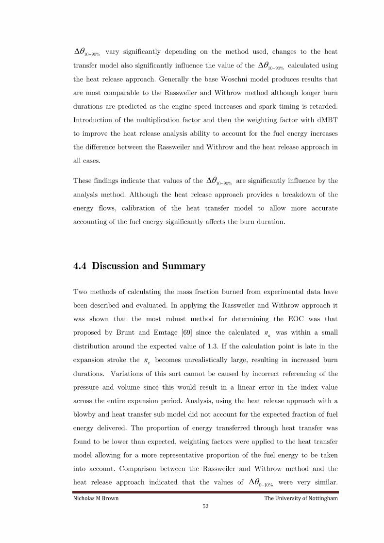
Nicholas M Brown The University of Nottingham
52
10 90% vary significantly depending on the method used, changes to the heat
transfer model also significantly influence the value of the 10 90% calculated using
the heat release approach. Generally the base Woschni model produces results that
are most comparable to the Rassweiler and Withrow method although longer burn
durations are predicted as the engine speed increases and spark timing is retarded.
Introduction of the multiplication factor and then the weighting factor with dMBT
to improve the heat release analysis ability to account for the fuel energy increases
the difference between the Rassweiler and Withrow and the heat release approach in
all cases.
These findings indicate that values of the 10 90% are significantly influence by the
analysis method. Although the heat release approach provides a breakdown of the
energy flows, calibration of the heat transfer model to allow more accurate
accounting of the fuel energy significantly affects the burn duration.
4.4 Discussion and Summary
Two methods of calculating the mass fraction burned from experimental data have
been described and evaluated. In applying the Rassweiler and Withrow approach it
was shown that the most robust method for determining the EOC was that
proposed by Brunt and Emtage [69] since the calculated en was within a small
distribution around the expected value of 1.3. If the calculation point is late in the
expansion stroke the en becomes unrealistically large, resulting in increased burn
durations. Variations of this sort cannot be caused by incorrect referencing of the
pressure and volume since this would result in a linear error in the index value
across the entire expansion period. Analysis, using the heat release approach with a
blowby and heat transfer sub model did not account for the expected fraction of fuel
energy delivered. The proportion of energy transferred through heat transfer was
found to be lower than expected, weighting factors were applied to the heat transfer
model allowing for a more representative proportion of the fuel energy to be taken
into account. Comparison between the Rassweiler and Withrow method and the
heat release approach indicated that the values of 0 10% were very similar.
Nicholas M Brown The University of Nottingham
53
Significant differences were found between values of 10 90% with in general the
heat release approach producing values greater than the Rassweiler and Withrow
method.
The choice of analysis method to determine the mass fraction burned by researchers
varies and without detailed knowledge of the method used, comparison of results is
impossible. Throughout this work the Rassweiler and Withrow method is adopted to
calculated the mass fraction burned using the Brunt and Emtage [69] method for
determining the ECO. Final consideration in this chapter is similar to the issues
raised with the calculation IMEPCOV in Chapter 3, where it was shown calculated
values were dependent on the number of cycles. Figure 31 shows the influence of
different cycle numbers to calculate 0 10%
COV and 10 90%
COV . At stable
operating conditions both parameters for the three engine speeds shown have
reached stable values with the minimum number of cycles (50) any increase in the
number of cycles results in insignificant changes to the values calculated. The trend
is repeated with the unstable operating conditions, the only exception being that the
required number of cycles to calculate a representative value of 10 90%
COV , where
it can be seen the number of cycles needs to be at least 200.
Nicholas M Brown The University of Nottingham
54
CHAPTER 5
Physical and Chemical limits of stable
operation
5.1 Introduction
Considered in this chapter are the parameters which limit stable operation in a
gasoline engine. Throughout the chapter IMEPCOV is used as the parameter to
describe the transition from stable to unstable operating conditions. Initial work by
Winborn [4] established that limits on stable operation of lean AFR mixtures at
various operating conditions could be characterised as a function of GFR for both
fully warm and cold operating conditions. The influence of spark timing was also
investigated, no change in the limiting value of GFR was found. Lai [5] expanded on
this work with the use of two diagrams, establishing both a rich AFR, bx and GFR
limits on stable operation. Only limited data was presented at spark timings
retarded from MBT*. The work presented in this chapter further develops the
diagrams presented by Lai [5]. Further understanding is provided as to the trends
observed and clarification of the limits of stable operation is provided by adopting
two testing methodologies. Finally, GFR as a parameter used to describe limits on
stable operation is compared to the thermal dilution parameter (TDP) defined by
[6] to rationalise stable operating range of a gasoline engine operating on different
fuel mixtures.
Nicholas M Brown The University of Nottingham
55
5.2 The influence of chemical and physical parameters on
cycle to cycle stability, initial testing
The results presented in this section were obtained using the test methodology
described in [4,5]. Firstly a stable (AFR 14.6) steady state test point is achieved
at a given throttle angle and valve timing. The fuel pulsewidth is then decreased to
increase the AFR (and GFR) until an unstable operating point is achieved, unstable
is defined as nIMEPCOV greater than 10 (this test methodology is defined as
‘constant air’). A discrepancy in the method of calculating nIMEPCOV exists between
[4] and [5]: misfiring and partial burning cycles5 were removed from the calculation
by [4] whereas [5] included all cycles, the implication being that at conditions where
misfiring cycles exist nIMEPCOV will be greater in the work presented by [5]. Here,
in this initial analysis, all cycles are included and therefore the data processing is
consistent with [5]. At each steady state condition a spark sweep is conducted to
ascertain MBT* spark timing, where the first data set is taken. To establish the
influence of spark retard on CCV two more data sets are taken with the spark
timing retarded from MBT* by 10 and 20oCA respectively.
The influence of chemical parameters, AFR, bx and relative spark timing was
investigated in 2 combustion stability diagrams. These two diagrams show the
boundaries of stable operation and show what parameters are involved in a way
which is diagrammatically clear.
The first /a bm m plotted against /f bm m results in straight lines of constant GFR
bounding regions of stability. From Chapter 3 equation 14.
a f b
f
m m mGFR
m
5 A misfiring cycle is defined as a cycle producing less than 5% IMEPn than the average. A partial burn
cycle is defined as producing less than 70% IMEPn than the average.
Nicholas M Brown The University of Nottingham
56
1 a b
f f
m mGFR
m m
1 a b b
b f f
m m mGFR
m m m
rearranging:
( 1) 1fa
b b
mmGFR
m m (55)
The burned gas in the unburned mixture during compression acts as a diluent, that
dilutes the fuel and air mixture. Once the amount of burned gas reaches a certain
limit, the air fuel mixture will become over diluted and combustion becomes
unstable. The second diagram is used to establish the burned gas fraction limit over
the range of AFRs tested. From equation 14, since
1
1 b
AFRGFR
x
rearranging:
1
b
GFR AFRx
GFR
1 11 AFR
GFR GFR (56)
Plots of bx against AFR as shown by equation 56 are straight lines provided GFR
is a fixed value. A stable region is formed by equation 56, burned gas fraction limit
and AFR limit. The two diagrams are used to represent data at three different
spark timings, MBT*, dMBT*=10 and dMBT*=20. These are shown in Figure 32,
Figure 33 and Figure 34. For a given relative spark timing there exists mixture ratio
limits that are dependent on both AFR and GFR. At MBT* operating conditions
the range of mixture ratios available for stable combustion are at a maximum, with
the stable operating range being bounded by a constant line of GFR = 24 for lean
Nicholas M Brown The University of Nottingham
57
and dilute mixtures, and an AFR = 10 for the rich operating limit. The stability
limits for high levels of dilution are better represented in Figure 33, which provides
zoomed in views of these areas for each spark timing. The bx limiting curve,
derived from Figure 34 intersects the rich limit as the dilution is increased up to the
maximum near to an AFR of 14, it is suggested that at high dilution levels,
0.27bx and lean mixture ratios, AFR>14.6 the stability limit can no longer be
described using GFR and that there is greater dependence on bx . Although similar
trends can be observed for both dMBT*=10 and dMBT*=20, the dilution and
mixture ratio limits are significantly reduced, particularly for the latter. For
dMBT*=10 the GFR limit is slightly reduced from 24 to 23, the rich limit remains
the same as for MBT*, with a notable change in the dilution limit, again the
maximum dilution for stable operation occurs at an AFR of 14. Significant reduction
in the stable operating mixtures occurs for dMBT*=20, the GFR limit is reduced to
19 and the rich limit although not as affected by the spark retard moves from an
AFR of 9 to 10. Again the most notable change is the dilution limit; the maximum
tolerable dilution is reduced to 20 percent across a similar AFR range. Figure 35
provides an overview of the limiting curves highlighting the significantly reduced
operating mixture ratios that can sustain stable combustion when MBT*=20.
Certain implications of the test method and analysis need to be raised, firstly, what
is the influence of removing misfiring cycles on nIMEPCOV , are these dominating the
reason for increasing nIMEPCOV ? The test method involves maintaining constant air
charge and reducing fuelling, therefore the average nIMEP reduces as the mixture
becomes lean, would this test method therefore affect the stability limit? The
influence of retarding spark timing could have a similar effect. Since the average
nIMEP reduces as the spark timing is retarded, would this reduction affect the
stability limit? Finally the use of nIMEPCOV , although this variable is representative
of variability of ‘useful’ work output from the engine, ultimately what the driver will
notice, to what extent is variability in combustion contributing to nIMEPCOV , since
nIMEPCOV takes into account variations in both combustion and the pumping work.
It is thought that variations in pumping work would be small compared to those
associated with combustion, but since the results come from a multi cylinder engine
Nicholas M Brown The University of Nottingham
58
and all the cylinders are not instrumented it is possible variations in pumping work
could become substantial as the cyclic variations increase. To what extent, though,
needs to be established.
To answer in part some of these questions another set of tests were conducted.
5.3 Evaluation of test methodology
The tests were not as expansive as previously shown, and the focus is the GFR ratio
limit rather than the bx or rich limit. In part the study was dictated by the fact the
bx limit could be reached only at low engine speeds, therefore providing insufficient
comparable data and that much work in both research and commercially focus on
lean burn technology. Three engine speeds were used 1000, 1500 and 2000rpm which
were typically encountered during the NEDC for this engine type, VO was
constant at each engine speed although varied between engine speeds to ensure
different initial bx . Effectively 3 operating conditions were investigated. *MBT
spark timing was established at each test point as described previously. To establish
the influence of test method on the stability limit constant air testing was
conducted, along with this method another method was used, instead of maintaining
constant air and reducing the fuelling to reach the stability limit the fuelling was
held constant and the throttle angle increased.
5.3.1 Influence of removing partial burning and misfiring cycles
from nIMEPCOV
Figure 36 shows the difference in nIMEPCOV for calculations involving all cycles and
those which are deemed not to have misfired or partially burned. As would be
expected when misfiring and partially burning cycles are removed the value of
nIMEPCOV and the rate of increase of nIMEPCOV reduces compared to the all cycles
case, this would in turn make it more difficult to determine the stability limit. Yet if
Nicholas M Brown The University of Nottingham
59
the limit was, as is here defined as where nIMEPCOV is greater than 10 then as can
be seen both figures indicate a similar GFR stability limit.
5.3.2 Comparison of stability limit from constant air and constant
fuel tests operating at MBT* spark timing
The influence on nIMEP and nIMEPCOV for the three engine speeds as the GFR is
increased is shown on Figure 37. The influence of the two different test methods on
nIMEP is apparent, where for constant fuelling nIMEP increases to a peak until the
point at which stability decreases, indicated by the associated increase in nIMEPCOV
where from that point onwards nIMEPCOV increases rapidly. As expected the
stability limit from the three engine speeds is the same. The constant air charge
results show that there is a linear decrease in nIMEP as the fuelling is decreased,
where there is a slightly earlier upturn in nIMEPCOV compared to the constant air
method, therefore it could be argued the results from this method would indicate
effectively a richer GFR stability limit. To further investigate this trend additional
examination of the data is presented. An alternative is provided in Figure 38 where
the data is re-plotted by removing the influence of changing nIMEP by looking only
at the change in variability by plotting the standard deviation (stdev) in nIMEP as
a function of GFR. Using the stdev in nIMEP the difference in the rate of
deterioration in stability as GFR is increased between the two test methods is
negligible. This suggests deficiencies in using the constant air method for
understanding and establishing stability limits, since part of the increase in
nIMEPCOV could be caused by the reduction in average nIMEP therefore not being
directly related to the presence of partial burning and misfiring cycles. Figure 39
shows when partially burning and misfiring cycles occurred for both test methods. It
is interesting that the point where the increase in nIMEPCOV occurs actually
corresponds to the point where partial burning cycles begin to be detected for both
test types and that for further increases misfiring cycles start to be detected.
Although the constant air test method results in a reduction in average nIMEP the

Nicholas M Brown The University of Nottingham
60
reason for increasing measured instability is due to the CCV. These results show
that when comparing results from the two different test methods, both result in the
same stability limit, but more importantly the occurrence of the instability is a
direct reflection of cycle to cycle variations and not a reflection of the change in
operating condition.
5.3.3 Validity of using net work output to characterise
combustion stability
As was raised earlier the combustion stability parameters shown have all been
derived from net work output, which is dependent on both variations in combustion
work and variations in the pumping work. The correlation between nIMEP and
gIMEP is shown in Figure 40 a, where the data for both constant air and fuel are
characterised by a single linear correlation, the correlation coefficients produce the
expected trend whereby higher gIMEP results in a smaller difference between
nIMEP and gIMEP due to reducing PMEP. Figure 40b shows the correlation
between nIMEPCOV and
gIMEPCOV . The gradient of the line of best fit indicates a
proportional offset between both parameters, where overall the nIMEPCOV is 25
percent greater than gIMEPCOV . This has significant implications with the data
presented since a substantial proportion of the measured variability arises during
the pumping stroke and is not directly related to variations in combustion. As
mentioned a reason for the difference could in part be attributed to variations in
pumping work. An alternative is the influence of signal-to-noise ratio on in-cylinder
pressure data.
The influence of signal-to-noise ratio will be unique to the rig and the method of
signal filtering adopted. Filtering was used here, where the method adopted was as
that of Shayler and Wiseman [68], where filtering is particularly necessary when
deriving combustion parameters namely the end of combustion. The Savitzky-Golay
filter used, effectively fits a polynomial through a segment of the unfiltered signal, in
this case a 3 third order polynomial was fitted every 11 measurement points

Nicholas M Brown The University of Nottingham
61
(5.5oCA), this smoothing period was chosen so as not to filter the high frequency
part of the pressure trace namely the peak pressure region. Figure 41 shows an
unfiltered and filtered pressure trace and the associated error ratio between the two.
There is significant high frequency noise on the pumping loop which decreases
during the power stroke, where the filtered data follows the unfiltered data with
very good accuracy indicated by the average error being 1. For the data sets
previously shown in this Chapter the difference in values of both nIMEPCOV and
gIMEPCOV between unfiltered and filtered in-cylinder pressure data is significantly
less than 1% indicating the signal filtering has not influenced the trend seen. It is
thought the contribution of variability from the pumping work will be higher for a
multi-cylinder engine due to the increased number of cylinder interactions occurring
compared to a single cylinder engine, but it is important to quantify this difference
to enable differentiation between combustion derived variability and that associated
to pumping work.
5.3.4 Comparison of stability limit from constant air and constant
fuel tests operating at spark timings retarded from MBT*
The two test methods investigated, constant air and fuel, were shown to produce
similar stability limits when chemical parameters were changed. Figure 34 highlights
the detrimental influence on stability when spark timing is retarded from the
optimum, yet again the reason for the increase in COV needs to be established to
ensure it is a reflection of combustion instability and not caused by the
experimental method. Figure 42 shows the influence of spark retard on gIMEPCOV
whereby for a given GFR increasing spark retard increases gIMEPCOV where as the
limiting GFR is approached the increase in instability for a given spark retard
becomes greater. Data at dMBT* of 15 and 20 were not captured at the last two
GFRs since the engine stalled at these conditions. Retarding the spark timing
reduces the average gIMEP , to investigate to what extent this accounts for
increases in gIMEPCOV is shown in two further figures. Firstly, Figure 43 re-plots

Nicholas M Brown The University of Nottingham
62
the data shown in Figure 42 where gIMEPCOV is replaced by stdev of gIMEP , this
indicates a similar trend as with Figure 42, although the increase in stdev of
gIMEP compared to gIMEPCOV with retarding spark timing is less at given GFRs,
this is more apparent at the richer GFRs. The reason for this trend is explained in
Figure 44. Increasing gIMEPCOV is caused in the case of spark timing changes by
increasing stdev of gIMEP and reduction in average gIMEP , the contribution of
both these factors to gIMEPCOV is quantified by calculating
gIMEPCOV by assuming
a constant value of average gIMEP defined by
*
_ *g
g
IMEP
g MBT
stdevIMEPCOV
IMEP (57)
Figure 44 shows the percentage difference in gIMEPCOV calculated using both
approaches. The contribution of reducing gIMEP is significant, particularly at the
maximum spark retard where approximately 35% of the value of gIMEPCOV results
from the associated reduction in average gIMEP . As the chemical stability limit is
approached this contribution reduces. This has an influence on gIMEPCOV and
affects the defined stability limits for the most retarded spark timings, where for
example the stability limit for dMBT = 20 would increase by approximately 1 GFR.
As a final comparison Figure 45 shows the change in stability limits with spark
retard, although there is some scatter all the data at a given relative spark timing is
characterised accurately with a single line where the reduction in stability limit with
increasing spark retard is apparent.

Nicholas M Brown The University of Nottingham
63
5.4 Comparison of parameters used to define stability
limits
Throughout this work GFR has been used to characterise stability limits, whereby
data from different engine speeds, loads, valve timings collapsed on to a single GFR
characteristic. Work by Tully and Heywood [6] investigated alternative parameters
that were particularly applicable with an engine operating on different fuel mixtures.
The first of two parameters was defined as the Volumetric Dilution Parameter,
VDP, representing the heat value per unit volume of the air/fuel mixture. The
second the Thermal Dilution Parameter, TDP, representing the heating value per
unit heat capacity of the air/fuel mixture, where combustion and emissions
parameters were found to correlate with TDP. For example, the parameter collapsed
on to a single characteristic the point at which combustion became unstable for
tests with different fuels and at different operating loads. The non dimensionless
parameter is given by:
_ , 1fuel onlyT
TDPT
(58)
where
.
.
f f
i
tot v
m LHV
Tm c
(59)
It is assumed the combustion process is modelled at constant volume and the change
in combustion composition is ignored, therefore vc = average heat capacity of the
unburned mixture. Where the mass weighted average vc was calculated from the
heat capacity of the individual components of the mixture at a representative
reference temperature. Figure 46 shows the performance of using TDP to define

Nicholas M Brown The University of Nottingham
64
stability limits. The data as with GFR collapses on to a single characteristic when
plotted using TDP, where the stability limit occurs at an approximate TDP value of
1.55, similar to the 1.57 found by Tully [6].
5.5 Discussion and Summary
The initial set of tests covered a wide range of operating conditions with the aim of
describing the chemical stability boundaries at 3 physical spark timings. The widest
set of boundaries, GFR limit 24, bx <0.27 and AFR > 9 was found at MBT* spark
timings. Only a small reduction in the boundaries occurred at dMBT*=10, where
the GFR limit was reduced to 23. When the spark timing was retarded by 20oCA
from MBT* the stability boundaries significantly reduced with a GFR limit of 19,
bx <0.2 and AFR > 10. This testing was termed ‘constant air’ testing since it
moved towards the stability limits by reducing fuelling while holding the throttle
angle constant. Issues with the test method and therefore the results were raised,
whereby the stability limit could be occurring early due to a combination of CCV
and lowering average nIMEP resulting in higher nIMEPCOV , hence a second set of
tests was conducted to validate the results from the first experimental set. Constant
air tests along with constant fuel tests were carried out, where constant fuel tests
increased the throttle angle to reach the stability limit. The results showed that the
stability limit was not influenced by the test method even though in the case of the
constant air tests there was a linear reduction in average nIMEP towards the
stability limit. It was found however that 25% of the nIMEPCOV is occurring in the
pumping stroke and therefore not directly related to CCV, where this difference will
be engine/rig specific, but it is recommended that when investigating CCV
gIMEPCOV should be used. The influence of spark retard on gIMEPCOV was
rationalised, whereby 35% of the increase at dMBT*=20 is accounted for by the
reduction in average gIMEP , in effect the magnitude of the CCV became greater
for a given gIMEP , although as the chemical stability limit was approached this
contribution reduced. As a comparison the results were plotted against TDP [6] this
parameter as with GFR collapsed the data on to a single characteristic. Combustion

Nicholas M Brown The University of Nottingham
65
stability has been shown to be a function of chemical and physical parameters, inlet
fuel/air/residual mixture fractions and spark timing respectively, a spark retard of
10oCA from the optimum does not significantly influence the stability limits whereas
a spark retard of 20oCA causes a marked reduction in stability limits.

Nicholas M Brown The University of Nottingham
66
CHAPTER 6
The Cause of Stability Limits
6.1 Introduction
The limits on stable operation reported in Chapter 5 were explored through the
study of variations in engine work output . IMEP provides information from the
entire cycle or only the combustion stroke if gIMEP is used, whereby variability
from only the combustion process can be indicated. Yet because IMEP is an
integral value over the combustion period it cannot provide any information on
which part of the combustion process is causing the variability, to establish this the
cylinder pressure information needs to be analysed and the associated mass fraction
burned calculated. In this Chapter, the aim is to establish the dominant part of the
burn that contributes to CCV. Establishing this link is important since it provides
valuable insight into which part of the burn is causing the variability in IMEP . To
understand which portion of the burn is dominant the mass fraction burn is broken
down into two sections, firstly the 0 10% and the rapid burn angle 10 90% . The
flame development angle encompasses the period when the flame develops from a
small kernel initiated by the spark to the point at which it has become fully
influenced by the turbulence within the cylinder, the fully turbulent flame then
propagates burning the majority of the cylinder mass during the rapid burn period.
The method adopted to determine the mass fraction burned was described in
Chapter 4.
Nicholas M Brown The University of Nottingham
67
6.2 The change in flame development and rapid burn
angle as stability limits are approached and exceeded
at MBT* spark timing
At MBT* spark timing both the constant air and fuel testing showed the chemical
limit was reached at a GFR of 24. The combined data is used here to investigate the
influence on mass fraction burned durations. Figure 47 shows the change in mass
fraction burn durations as GFR is increased for the three engine speeds investigated
previously, all at MBT* spark timing. The shortest burn duration in both cases
occurs at the minimum GFR (in this case this is equivalent to a stoichiometric
AFR). As the GFR ratio is increased both the 0 10% and the 10 90% increase,
whereby the 0 10% increases at approximately a constant rate to the maximum
GFR value, with the 10 90% relatively unaffected with the initial increase in GFR
but more rapidly increasing in duration once the GFR exceeds 21. Interestingly, the
two burn durations increase from similar minimum values, 22oCA to maximums of
45oCA. The increase in mass fraction burn duration for these sets of tests is
essentially caused by changes in the laminar burning velocity. Although the burning
process within the cylinder is turbulent, the increase in GFR for the tests shown has
no influence on turbulence since the engine speed and valve timing remain constant,
hence there will be no change in turbulent burning velocity apart from the change
embodied in the laminar burning velocity.
The laminar burning velocity is a function of temperature, pressure and mixture
ratio. Work by Rhodes and Keck [78] found an empirical relationship describing the
influence of all the parameters mentioned above, based on constant volume bomb
experiments, whereby the laminar burning velocity ( uS ) is given by;
0.733(1 2.06 )uu uo b
o o
T pS S x
T p (60)
Nicholas M Brown The University of Nottingham
68
where uoS is the undiluted laminar flame speed,
oT the referenced temperature
(298K), op reference pressure (1 atmosphere),
uT unburned gas temperature, p
actual pressure and bx volume fraction of diluent.
An estimate of the change in laminar burning velocity as the GFR is increased is
given in Figure 47. The calculation of uS assumes the unburned gas undergoes
adiabatic compression, whereby the calculated uT is based on measured cylinder
pressure with the initial cylinder temperature at the start of compression assumed to
be that of the measured inlet manifold temperature. Mixture ratios are based on
measured parameters, where the values are calculated from methods discussed in
Chapter 3. The values plotted are the inverse of uS normalised at nominally the
same GFR. In both plots, a and b, uS is an average value, whereby the calculated
values are the mean average value during either the 0 10% or 10 90% . The
change in uS in both cases is very similar. This is effectively caused by the
dominant influence of the mixture fraction in these calculations, and also that the
combustion process is phased to maintain MBT* spark timing. The second effect
means that each part of the combustion process will see similar temperatures and
pressures although the change in mixture fraction towards more lean regimes
reduces the absolute values. Figure 47 provides an overview of the combustion
process; as the mixture ratio moves towards and exceeds stability limits, both the
0 10% and 10 90% both increase, approximately doubling over the range shown
(~20oCA to 40oCA 18-27GFR). This does not provide information on the cause of
stability limits, however increasing combustion duration does not directly indicate
the combustion process is likely to be more unstable, stability limits are caused by
variability between combustion events, not simply by a longer burning process.
Understanding which part of the combustion process is responsible for stability
limits in terms of work output, IMEP , the normalised variability in 0 10% and
10 90% are plotted in Figure 48. Figure 48a indicates that there is a relatively
small change in 0 10%COV as the stability limit is reached and exceeded, where it
could be argued that taking the scatter into account there is actually no change in
the variability, it is also worth noting that the approximate value of 0 10%COV is
Nicholas M Brown The University of Nottingham
69
7% across the entire range of GFR. Both the magnitude and change in 10 90%COV
are much more substantial than those seen for 0 10%COV . Figure 48b indicates that
not only is the variability of 10 90%COV greater than that associated with 0 10%
COV
the increase in variability is significant, nearly trebling as the stability limit is
reached and surpassed. In Chapter 5 issues were raised relating to the use of COV ,
these are applicable here although the influence is the inverse, in both cases the
average burn durations increases therefore the instability indicated by calculating
COV will be lower than if the duration had remained constant. Figure 49a and b
shows the change in standard deviation of the 0 10% ( 0 10%stdev ) and 10 90%
( 10 90%stdev ). There is a distinct difference between Figure 49a and Figure 48a,
whereby there is a notable increase in the 0 10%stdev , there is a similar pattern
between Figure 49b and Figure 48b indicating the increase in variability of the
10 90% is still greater than that of 0 10% . The fact that Figure 49 suggests an
apparent correlation between the variability of 0 10% and 10 90% is further
investigated in Figure 50. The correlation between increasing variation in the
10 90% and 10 90% is significant, whereby the correlation coefficient is
approximately 0.7, though this appears to break down at the same point when the
stability limit is reached and exceeded (at 0 10% 4stdev ). Yet, the general
correlation suggests that the move towards less stable combusting cycles is
manifested in changes in the 0 10% where the instability is further magnified in
the 10 90% , with approximately a 3 times increase in instability in the 10 90%
compared to the 0 10% . The source of CCV appears to lie in the variability of the
0 10% phase and is magnified in the 10 90% .
Previous work [31,79,80] investigated the causes of cyclic variability, as with much
of the research carried out in this field a number of different parameters were used,
not just burn rates and the associated variations. All compared experimental results
with models of differing complexities. In the case of [31] the simulations suggested
that 25% of the standard deviation of combustion duration, IMEP, maximum
pressure and maximum pressure location was caused by ‘random walk’ of the flame
kernel operating at stoichiometric conditions. Although this value is less than that
found from the experimental work presented here the order of magnitude is similar,
although some caution should be used in comparing these results due to the
Nicholas M Brown The University of Nottingham
70
different factors used. The work presented by [79] concluded that displacement of
the flame kernel during the early stages of combustion has a major part in the
origination of cycle to cycle variations, again many factors were used to assess the
variations, including 0 10%COV and 10 90%
COV . The modelled results from [80]
provided a fundamental appreciation of the causes of the variability during early
stages of flame development, whereby initially the flame burns with a rate close to
laminar flame speed, yet as the flame grows the influence of turbulence increases
until a point where the flame is a fully developed turbulent flame. The work showed
that the flame development period is most susceptible to flame stretch, where
excessive flame stretch can lead to unstable burning and eventually the flame will
quench. Flame stretch is characterised by the Karlovitz number, representing the
ratio of chemical to eddy lifetime. In effect a high Karlovitz number indicates high
flame stretch, therefore a less stable flame. It was shown that for the initial flame
development process flame stretch for lean mixtures can enter regions of partial
quench therefore resulting in less robust initial flame propagation. It is likely a
combination of the factors discussed above will increase the cyclic variations seen in
the results shown but it does appear that variability in the initial flame
development is magnified during the propagation phase.
6.3 The change in flame development and rapid burn
angle as stability limits are approached and exceeded
at dMBT* spark timing
An increase in instability was shown to occur as the spark timing was retarded,
although the absolute level of instability was shown to be amplified when using
COV parameters since there was a reduction in average work output not just an
increase in CCV. The influence on burn rate parameters is initially shown in Figure
51, with the change in 0 10% and 10 90% duration plotted as a function of GFR
for a range of spark retards (sub plots a and b are a repeat of Figure 47 and are
Nicholas M Brown The University of Nottingham
71
shown to ease comparison). Dealing with the 0 10% first, the change in relative
spark timing is shown to have an interesting trend, whereby if the spark timing is
retarded from MBT* by 5 degrees there is a slight reduction in 0 10% that
becomes most notable at the highest GFR. There is a significant change in the
0 10% when the dMBT*=10, with a reduction in 0 10% of approximately 25%
at the highest GFR. There is also a change in the shape of the curve with the
gradient moving from an increasing duration as seen with MBT* and dMBT*=5 to
a flat profile, whereby the changes in GFR no longer influence the 0 10% . For the
final two spark timings dMBT*=15 and dMBT*=20 the trend is similar to that
seen for dMBT*=10 although there is an increase in duration and a slight upturn in
gradient the absolute burn durations are still lower than those seen at MBT* and
dMBT*=5. This trend is predominantly caused by the relative location of the
0 10% and the associated change in thermodynamic conditions. Spark retard
results in the 0 10% moving closer to TDC where the unburned gas temperature
is higher than at MBT*, the result is that the associated uS is greater manifesting
in reduced 0 10% . The results suggest that a spark retard of 10 from MBT*
results in cylinder thermodynamic conditions that produce the most rapid and
consistently the most rapid 0 10% across the wide range of GFR.
The results for the 10 90% are contrary to those shown for 0 10% and in many
respects are more simple. Generally there is an increase in 10 90% as the spark
timing is reduced from MBT*, with the increase reaching a maximum with a spark
retard of 20. The trend of increasing duration as GFR is moved to leaner conditions
is maintained as the spark timing is retarded. Scatter in the data increases as the
spark timing is retarded, this reflects the generally unstable nature of the
combustion process at these conditions. The two types of tests, constant air and fuel
indicate similar relationships with spark retard for both the 0 10% and the
10 90% .
As with the MBT* data to understand which part of the combustion event is
causing a reduction in cycle stability, plots of 0 10%COV and 10 90%
COV are shown in
Figure 52, for completeness the MTB* is re-plotted as a datum. As the spark timing
is retarded from MBT* the change in 0 10%COV is marginal for a given GFR, it is
Nicholas M Brown The University of Nottingham
72
only once dMBT*=15 that there is a notable increase in 0 10%COV , where for a
given GFR the trendline suggests 0 10%COV is increased by ~30%. At dMBT*=20
there is a further ~30% increase in 0 10%COV compared back to dMBT*. It should
be noted though that the scatter in the data increases at the extreme spark retards
and therefore it could be suggested 0 10%COV is no longer a function of GFR. The
influence of spark retard on 10 90%COV follows a more consistent trend whereby as
the spark timing is retarded for a given GFR there is always (as shown by the
trendline) an increase in 10 90%COV , as with the 0 10%
COV there is a reasonable
amount of scatter in the data particularly at the maximum spark retard. For
completeness the change in 0 10%stdev and 10 90%stdev is shown in Figure 53. The
change in 0 10%stdev is reasonably consistent, whereby with retarded spark timing
at a given GFR there is an increase in 0 10%stdev , at the maximum spark retard,
the data shows the 0 10%stdev is insensitive to GFR whereby the level of variability
is greater than that for all other spark timings but there is no increase as the GFR
ratio is increased. The change in 10 90%stdev follows a more expected trend, with a
significant increase in 10 90%stdev with GFR, whereby the absolute level of
variability is increased as the spark timing is retarded from MBT*.
Figure 54 correlates 0 10%stdev and 10 90%stdev . At MBT* spark timing the
increase in variability of the 0 10% is directly proportional with that of 10 90% ,
for retarded timings the same statement holds yet the correlation between the two is
significantly reduced for the maximum retarded spark timings. At a spark retard of
10oCA the 10 90%stdev increases for a given 0 10%stdev but once the spark timing is
retarded by 10oCA any additional spark retard results in the same 10 90%stdev for a
given 0 10%stdev , in effect the maximum level of 10 90%stdev has been realised.
6.4 Discussion and Summary
Greater understanding of the causes of CCV have been established in this chapter
by correlating combustion parameters 0 10% and 10 90% and the associated
variations in these parameters with GFR. Increases in burn duration have been
Nicholas M Brown The University of Nottingham
73
shown to directly correlate with increases in CCV, this is predominantly caused by
variability in 0 10% which is translated into greater variability in the 10 90% , in
effect the source of the variability is manifested in the 0 10% and does not start
occurring in the 10 90% . The influence of spark timing changes has been
described, whereby the changes in 0 10% are different to those of 10 90% as the
spark timing is retarded. The 0 10% decreases significantly as the spark timing is
retarded from MBT* to a minimum at dMBT*=10, caused predominantly by the
more favourable thermodynamic conditions, since the 0 10% is occurring closer to
TDC where the unburned gas temperature is greater than if the spark timing is at
MBT*. Although the 0 10% reduces in duration the actual variability increases as
the spark timing is retarded to a maximum at the maximum spark retard. The
characteristics of the 10 90% are much more straight forward, as the spark timing
is retarded both the duration and variability increase again to a maximum at the
maximum spark retard. The cause of combustion variability is similar between
MBT* operating conditions and retarded spark timing cases, the combustion
variability starts in the 0 10% and is amplified during the 10 90% . Although for
significant spark retards, >15oCA the correlation reduces, indicating increased levels
of instability occurring in the 10 90% .

Nicholas M Brown The University of Nottingham
74
CHAPTER 7
Emissions Characterisation
7.1 Introduction
Current European legislation on pollutant emissions from spark ignition engines sets
limits on emissions of carbon monoxide (CO), unburned hydrocarbons (HC’s) and
oxides of nitrogen (NOx). The main reason to restrict, specifically these emissions is
their toxicity and the detrimental impact they have on the environment [81].
Legislation restricts the emissions per kilometre (km), determined over a
representative drive cycle, for example the NEDC, which all new vehicles must
adhere to. The use of a vehicle model that predicts emissions flow rates accurately is
therefore a very powerful tool that can be used to assess the required performance of
the vehicle aftertreatment system.
The emissions work here focuses on the characterisation of engine out pollutant
emissions in the exhaust gas stream of a PFI engine, not emissions formation in
cylinder. The engine was operated with variable valve timing, at stable and unstable
combusting conditions. The methodology uses the connections between exhaust
emissions and engine global parameters such as AFR, bx and spark timing relative
to the optimum. Emissions are more sensitive to changes in operating conditions
with for example a few degree changes in spark timing resulting in a small decrease
in torque but a doubling of pollutant emissions. An alternative approach using NOx
emissions to determine spark timing relative to MBT* is highlighted and evaluated.
The impact of deteriorating combustion stability on emissions is investigated and
decoupled from normally occurring emissions. Physical underpinning of forms of
generic functions is deferred until Chapter 8.

Nicholas M Brown The University of Nottingham
75
7.2 Characterisation of Emissions and Previous Work
Exhaust emissions based on measurements of molar volumetric concentrations in the
exhaust gases vary with engine speed, load, AFR, spark timing and EGR rate.
Normalising values provides a useful comparison of data and aids the direct
comparison of emissions from different engines. The normalised value is termed the
emissions index, defined as:
gas
gas
fuel
mEI
m
(61)
where gasm refers to the particular emission in question, for this study CO, HC’s
and NOx.
Emissions concentrations are sensitive to a small set of particular engine parameters
and have been shown to produce repeatable trends from one engine to the next.
Shayler et al [7] developed a set of ‘generic functions’, based on a number of
independent variables, namely AFR, spark timing relative to the optimum and the
bx . The functions were derived from analysis of a large database of experimental
data from four-valve cylinder DOHC engines with typical pentroof, open chamber
features. The functions were successfully used by Horn [82] to predict emissions
accurately for a Mitsubishi DISI engine operating in homogenous charge mode.
Although the emissions from the same engine operating under stratified mode were
described using trained neural networks.
The trends characterised were found to be universal and adjustments where
necessary were simple scaling factors of the original functions. The original functions
derived by [7] and modified functions used to characterise the Jaguar AJ27 where
necessary are shown in Table 4 referred to as Series 1 and Series 2 respectively. The
form of the generic equations and values for the constants are provided in Table 5
and Table 6.
Nicholas M Brown The University of Nottingham
76
7.3 Generic Representation
7.3.1 CO Emissions Index
Carbon monoxide emissions are a function of equivalence ratio. Under lean
operation there is sufficient oxygen to oxidise the CO to CO2 but CO remains in the
exhaust due to limiting chemical reaction rates as discussed in Chapter 8. CO is
present in the exhaust gases during rich operation due to insufficient oxygen. Figure
55 shows the fit of Jaguar AJ27 data to both Series 1 and Series 2. The correlation
when the engine operates rich is excellent, as found by Horn [82] Series 1 under
predicts COEI for lean operating points, the alternative function Series 2 shows
improved correlation with these points as highlighted by Figure 56. There is no
noticeable change in COEI with varying intake cam timing. Siewert [83], made
similar findings when operating a single cylinder engine with two extreme intake
valve opening times. Although these findings are contrary to Leone et al [43] that
stated the early intake valve opening intake turbulence decreases, increasing mixture
charge inhomogeneity resulting in higher CO emissions.
The generic functions were previously fitted to data sets where there was no
information about the combustion stability. Using nIMEPCOV as a method of
distinguishing between unstable and stable combustion operating points the
contribution of ‘normal’ emissions and those resulting from unstable combustion can
be decoupled. Figure 57 shows the effect of combustion instability on COEI , the
trend in CO emissions remains the same as for the stable operating points. This is
highlighted in Figure 58 by the comparison of the measured and predicted COEI at
unstable and stable operating conditions, where it is shown that there is no
significant deviation due to increasing instability.
Nicholas M Brown The University of Nottingham
77
7.3.2 HC Emissions Index
Hydrocarbon emissions index is a function of equivalence ratio and relative spark
timing. The original generic function work found that HCEI was approximately
proportional to GFR which is used here as a starting point. The change in the
relative emissions index ( /HCEI GFR ) with equivalence ratio is shown in Figure
59. The data from the AJ27 comprises only experimental points where the VO was
fixed to 15oCA and nIMEPCOV < 4.0. These constraints are applied since this is a
typical VO period for conventional SI engines [84] and combustion instability
increases the hydrocarbon emissions (discussed later), thus ensuring the changes in
hydrocarbon emissions are only a function of equivalence ratio. Although it is
evident that there is a significant spread of data, due to experimental scatter and
the limitations of a simple equivalence ratio function, the Jaguar AJ27 data is
shown to follow the original function with no less accuracy than the original PFI
engine data. The shape of the curve is dictated by oxygen availability and bulk gas
temperature. Under rich operation 1.4 HC emissions account for only 3% of the
fuel burned although there is 40% excess fuel, CO accounts for the significant
proportion of excess fuel with H2 the remainder. Lean combustion and therefore
lower temperature causes an increase in HC emissions due to the reduced rate of HC
oxidation to CO, this is further discussed in Chapter 8. The correlation between
GFR and HCEI is investigated in Figure 60 and Figure 61. The correlation between
HCEI and equivalence ratio is very similar to that shown for relative HCEI ,
therefore a generic function was created to predict HCEI as a function of
equivalence ratio. Comparing measured and predicted error ratio for this generic
function against GFR shows that under stable operating conditions the correlation
is poor, R2 = 0.0542.
The influence of VO on HCEI is shown in Figure 62 by comparing the error ratio
correlation of measured and predicted as a function of VO. Increasing VO produces
a notable reduction in HCEI with the maximum reduction of approximately 20% at
the maximum VO. The reason for the reduction was hypothesized by [43] where the
increased VO period causes gas to backflow into the intake port and is therefore
drawn back into the cylinder during the intake stroke where the unburned
Nicholas M Brown The University of Nottingham
78
hydrocarbons are ‘re-burned’. A study by Seabrook et al [85] using a fast flame
ionisation hydrocarbon detector placed in the exhaust port showed that due to the
VO period, significant back flow occurs from the exhaust port into the intake port.
The backflow significantly reduced the final hydrocarbon peak associated with the
exhaust process.
The final part of the generic function for hydrocarbon emissions is the effect of
spark timing. Altering the spark timing phases and changes the duration of the
combustion process. Rationalisation of the influence of spark timing changes are
achieved by referencing spark timing to the optimum values at MBT*. Figure 63
shows the influence of spark timing on normalised HCEI . The correlation between
the generic function and the data set is excellent. The influence of AFR is as was
previously found; the effect of external EGR could not be evaluated since the engine
did not have an external EGR system. The effect of EGR previously, was similar to
reducing AFR, where the reduction in HC emissions due to retarded spark timing is
less because of lower expansion and exhaust port temperatures. The combined
performance of the HC generic function is shown in Figure 64, although each
individual part of the generic function contributes errors, overall the predictions are
within 30% of measured values.
Combustion instability is associated with poor driveability and an increase in HC
emissions, due firstly to lower combustion temperatures reducing post flame HC
oxidation both during expansion and in the exhaust port, followed by partial burn
and then misfiring cycles. The effect of combustion instability is shown in Figure 65;
the deviation from the generic function is significant with in some cases the HCEI
exceeding 100% of the predicted value. In these cases combustion stability limits
were exceeded by operating the engine past the lean or dilution limits. Combustion
instability limits can also be reached and exceeded by retarding the spark timing
from the optimum, this effect is shown in Figure 66. Where under stable operating
conditions spark retard reduces HCEI , spark retard that results in reduced
combustion stability increases the HCEI from the minimum occurring at MBT*.
Rationalisation of the influence of combustion instability on HCEI is shown in
Figure 67, where the increase in HCEI due to both chemical and physical factors is
Nicholas M Brown The University of Nottingham
79
described by a single linear function of nIMEPCOV . Determining the point at which
HCEI starts to increase due to combustion instability is hard to define due to
scatter of experimental data. A reasonable approach to gaining some insight is to
evaluate the point at which the equivalence ratio function and the nIMEPCOV
function intersect at a given equivalence ratio. At an equivalence ratio of 1.0 the
intersection point is equivalent to a nIMEPCOV of 2.5, although the spread of data
about this point suggests nIMEPCOV between the range of 2.5 - 4. The upper limit is
chosen here.
Application of the HCEI generic function falls into two parts, stable and unstable
with the switching point between the two defined as nIMEPCOV >4. In the stable
region HCEI is a function of equivalence ratio, relative spark timing and VO. For
nIMEPCOV >4 HCEI is predicted using the base equivalence ratio function with the
addition of the linear function of nIMEPCOV . The overall performance of the HC
generic function is shown in Figure 68 where again the majority of the predictions
are within 30% of the measured values.
7.3.3 NOx Emissions Index
NOx emissions are predominantly a function of the burned gas temperature and
oxygen availability, these factors can be described using AFR, GFR and relative
spark timing. Figure 69 shows the agreement between the measured and the
predicted NOx emissions index over a range of AFR and GFR at MBT*. The trends
are consistent with previous work [7], although the overall prediction was
approximately double the measured values across the entire operating range. A
constant correction factor as shown in Table 4 is applied to all predictions. There is
no noticeable direct effect of VO on xNOEI as shown in Figure 70, changes in VO
have been shown to significantly influence the residual gas fraction, and these are
accounted for in the generic function by GFR. As with HCEI , xNOEI is
substantially affected by changes in spark timing relative to the optimum as shown
in Figure 71. The original function fitted to engine data by Shayler et al [7] is shown
Nicholas M Brown The University of Nottingham
80
to under predict xNOEI when the spark timing is advanced from MBT*, the reason
for this is that the original function was fitted to experimental data with engines
operating up to dMBT values of –10. For dMBT < 20 the generic function provides
a very accurate prediction, if dMBT ≥ 20, xNOEI remains at a constant value of
approximately 0.12. The influence of combustion instability on xNOEI at MBT* is
shown in Figure 72. From Figure 73 it is apparent that reducing combustion
stability leads to a reduction in xNOEI , the reduction is not predicted by the
current generic function. There is a greater reduction in xNOEI due to increasing
bx than was previously found, essentially due to the increased data set at the
unstable combustion conditions. The prediction of the generic function is improved
at these conditions without reducing the accuracy at stable operating points by
altering the bx constant as shown by the comparison of Figure 73 and Figure 74.
Reduction in xNOEI from spark retard that also results in reduced combustion
stability follows the original generic function as shown in Figure 75. The predictions
of xNOEI generally fall within the 30% error, with less scatter exhibited than with
the HCEI generic function, due essentially to the more simplistic formation
mechanisms of xNOEI emissions than HCEI .
7.4 Assessment of emissions models over the NEDC
The influence of the models developed in the previous sections have been assessed
using NuSIM, a vehicle simulation model whereby the engine system has been
modelled based on experimental data. The engine controller was defined based on a
prototype production controller designed by Jaguar. Figure 76 shows a comparison
between the original emissions models and those based on the measurements from
the AJ27, both real emissions flow rate and cumulative emissions are shown. Figure
77 shows a difference plot whereby new minus old emissions predictions are
presented highlighting more easily the differences. There is generally no difference in
CO emissions due to the model predicting the engine running most of the drive cycle
slightly rich of stoichiometric. Of particular note is the significant difference between

Nicholas M Brown The University of Nottingham
81
the models in relation to the HC emissions, whereby the new model indicates
increased HC emissions during both transient and steady state operation. The
increase is caused by the additional contribution of unsteady combustion HC
emissions, where during the transients the nIMEPCOV is increasing to values in
excess of 25 with certain steady state periods the engine predicted to be operating
with a nIMEPCOV of approximately 15. The cause of the high
nIMEPCOV is
predominantly due to the engine running with large valve overlaps increasing the
bx to levels that are exceeding the stability limit. The change in NOx emissions is
small but generally lower than the old model due to the correction factor applied
and the high levels of bx during steady state operation.
It is unlikely that a production variant of an engine controller would result in engine
excursions and steady state conditions causing such increases in HC emissions. The
model does show the importance of accurate engine calibration to avoid unnecessary
increases in HC emissions.
7.5 Alternative Approach to Determining MBT*
Typical engine management systems (EMS) are calibrated to maintain spark timing
as close to MBT* as possible, since this timing corresponds to maximum brake
power and minimum brake specific fuel consumption. The exact location of MBT* is
often hard to determine due to the relative flatness of the torque curve. Further
problems can arise when determining MBT* spark timing when spark sweeps are
knock limited, the method described in Chapter 3 to determine MBT* can
frequently result in over extrapolation of MBT* under these conditions as shown in
Figure 78. Although advancing or retarding spark timing from MBT* adversely
effects brake specific fuel consumption, there is much more of a notable effect on
HCEI and particularly xNOEI , for example retarding the spark timing by 4oCA
from MBT* increases the brake specific fuel consumption by 6% but reduces xNOEI
by 23%. Therefore knowledge of spark timing relative to MBT* is much more

Nicholas M Brown The University of Nottingham
82
important from the emissions perspective. An alternative method for determining
MBT* from xNOEI is investigated.
There are two possible methods for determining MBT* from xNOEI . Firstly using
the xNOEI trend from a spark sweep, or applying the generic functions to a single
data point whereby the expected error between torque and xNOEI derived MBT*
would be 30%. The first method utilises the robust correlation between spark timing
and xNOEI as shown in Figure 71. Investigating this correlation further for data
only at stoichiometric conditions xNOEI exhibits a linear increase for dMBT < 16
as shown in Figure 79. The excellent linear correlation between dMBT < 16 and
xNOEI is shown to apply over eight individual spark sweeps. The accuracy is
increased if as would be the purpose of using this method, the correlation was
applied only for one spark sweep. Application of this method requires a linear line of
best fit through the data set, the most retarded spark timing xNOEI value is
assigned the constant value line, where the straight line intersects the constant line
the actual spark timing has a relative spark timing of 16 (MBTD = 16), an example
is shown in Figure 80. This method has limitations, the spark sweep ideally should
have data points retarded more than MBTD = 16 so that an accurate crossing point
can be determined and as shown in Figure 80 and the method itself can only be
applied to spark sweep data. The method has been shown to have an accuracy of
predicting MBT* to within 3oCA from MBT* evaluated using the torque based
method.
7.6 Combustion Efficiency
The development of the generic functions including unstable combustion data has
lead to an investigation of combustion efficiency since it was likely that previously
developed trends would no longer be applicable. Combustion efficiency is defined by
Heywood [14]:

Nicholas M Brown The University of Nottingham
83
1
[ /( )]
i
f
i LHV
ic
f a f LHV
x Q
m m m Q (62)
where the mass fractions ( ix ) are CO, hydrogen (H2), HCs and particulates
(assumed to be zero in a SI engine) and iLHVQ are the lower heating values of these
species. Where the heating values for CO is 10.1MJ/kg and H2 is 120MJ/kg, the
lower heating value for HCs is assumed to be the same as the fuel, 44MJ/kg.
Shayler and Chick [86] modelled c using the data presented by Heywood [14] using
the following functions
0.98c (63)
for less than one, and by
22.662 2.26 0.577c (64)
for greater than one. Reducing combustion stability leads to increasing HC
emissions and therefore reduced c , the AJ27 data was used to calculated the c ,
where H2 was calculated from the water gas shift reactions based on the measured
and determined exhaust gas concentrations of CO and CO2 and H2O. Figure 81
shows that c is significantly influenced by bx . With the lowest levels of bx the c
follows the previously developed function, where a significant reduction in c occurs
when the mixture becomes rich due to incomplete combustion and therefore the
presence of CO. As the mixture becomes increasingly lean ( 0.73) the
combustion stability limits are reached and then exceeded, HC emissions increase
rapidly, reducing the c . As the bx is increased the lean limit where c reduces,
Nicholas M Brown The University of Nottingham
84
moving towards stoichiometric conditions where the combustion process is most
robust, this trend continues until the bx > 0.25 where across the entire equivalence
ratio range c is offset from the fitted trend. Further increase in bx leads to
extremely unstable combustion, ultimately causing the engine to stall.
7.7 Discussion and Summary
Feedgas Emissions including combustion efficiency have been successfully described
using generic functions where the functions have been further developed to include
the influence of unstable operating conditions and valve overlap. CO emissions were
shown to be accurately characterised by a single function, whereby there was no
need to include functions for the influence of valve overlap and differentiating
between stable and unstable operating conditions. HC emissions are more complex,
due to the numerous contributory sources within the cylinder and the complex
formation and consumption that occurs during the combusting stroke. Again the
general form of the functions were applied, although the dependence on GFR was
disregarded, it is thought the inclusion of GFR in the original function aided
collapsing unstable combusting conditions on to the function, whereas in this
case unstable combusting conditions were described separately. For stable operating
conditions changes in valve overlap had a significant influence on HC emissions,
where from the datum overlap of 15oCA to the maximum valve overlap of 42oCA
HC emissions reduced by approximately 20%. The influence of relative spark timing
was shown to follow previous trends. The influence of deteriorating combustion
stability on HC emissions was established whereby there was a deviation from the
predicted HC emissions when nIMEPCOV was greater than 2.5-4, where the increase
in HC emissions with nIMEPCOV followed the same trend whether
nIMEPCOV was
increased by chemical ( bx and AFR ) or physical means (changes to relative spark
timing). NOx emissions are described using the originally developed functions with
minor changes to improve the predictions. There was no direct influence of valve
overlap on NOx emissions. The reduction in NOx emissions with valve overlap was
described by the increase in bx . As with CO emissions the inclusion of unstable

Nicholas M Brown The University of Nottingham
85
operating conditions did not require additional functions. The robust correlation
between relative spark timing and xNOEI was shown and a method for determining
relative spark timing based on xNOEI rather than the traditional torque based
approach, where the results showed both methods would produce MBT* spark
timing within 3oCA from each other.
The final part of this chapter dealt with combustion efficiency determined from the
emissions. The experimental data showed that with an engine with variable valve
timing the traditional functional form of combustion efficiency as a function of no
longer holds true. It is necessary to take into account the change in combustion
efficiency with bx and that for a given equivalence ratio combustion efficiency can
be substantially reduced by high levels of bx , this is a direct reflection of the results
shown in Chapter 5.
Nicholas M Brown The University of Nottingham
86
CHAPTER 8
Emissions Generic Function Physical
Underpinning
8.1 Introduction
The generic functions to describe the emissions from SI engines developed in
Chapter 7 were based on measurable engine parameters such as AFR and bx , with
the specific application to predict emissions for a vehicle model. This chapter
underpins the functions developed by comparing the results with more
fundamentally based approaches, including literature reviews relating to each of the
emissions. Typically these types of approaches are used with thermodynamic
simulations of the cylinder, where the combustion process is modelled along with
emission formation on a crank resolved basis, these methods can be used relatively
successfully to predict CO and NOx emissions, whereas the complexities involved
with HC formation and consumption mean the models tend to be highly complex.
Results from such simulations are compared with the generic functions providing
underpinning of the form the functions have taken.
Nicholas M Brown The University of Nottingham
87
8.2 Calculation of cylinder temperature and gas species
The major species of combusted hydrocarbon fuels at low temperatures are N2, H2O,
CO2 and O2 or CO and H2. At higher temperatures, approximately greater than
2200K, these major species dissociate and react to form additional species. The
concentration of each species given sufficient time will reach an equilibrium level,
where the production and removal of each species is at equal rates. The second law
of thermodynamics defines the criterion for chemical equilibrium, for complex
chemical equilibrium compositions, such as required here, standardised computer
methods are available [87], commonly known as the NASA-Lewis method. The
method used to calculate flame temperatures and equilibrium species here is a
simplified approach, as developed by Olikara and Borman [88].
8.3 CO Emissions
CO formation is one of the principle reaction steps in the hydrocarbon combustion
mechanism, summarised by [14]
2RH R RO RCHO RCO CO (65)
where R stands for the hydrocarbon radical. The CO formed in the combustion
process is then oxidised to CO2 at a slower rate. The principle reaction being
2CO OH CO H (66)
Figure 82 shows the COEI generic function and equilibrium COEI at three points in
the cycle. Firstly equilibrium COEI at average peak burned gas pressures and
Nicholas M Brown The University of Nottingham
88
temperatures, where the temperature is defined as adiabatic flame temperature
evaluated at measure peak cylinder pressure. Secondly equilibrium COEI evaluated
at the end of expansion temperatures, the temperature has been assumed to be
constant, at 1800K [84], across the equivalence ratio range. Finally equilibrium
COEI calculated at measured exhaust port temperatures. The measured
concentration of COEI is lower than the peak cycle temperatures and pressures but
is higher than equilibrium values for the exhaust port conditions near to
stoichiometric and lean conditions. This indicates the formation and removal of CO
in the exhaust, is kinetically controlled, the drop in temperature and pressure
caused by the expansion process is at a faster rate than the time constants of the
controlling reactions, therefore CO does not remain locally equilibrated.
A study by Newhall [89] investigated the oxidation of CO during the expansion
stroke by carrying out a series of kinetic calculations assuming the burned gas at the
time of the peak cylinder pressure was uniform and in equilibrium. The study found
that although reaction (66) is slow compared to many of the precursor hydrocarbon
reactions it is sufficiently fast enough to be continuously equilibrated throughout
expansion, this indicates that reactions producing OH and H must be themselves
involved in rate limited reactions. The reactions studied, firstly the bimolecular
atom exchange reactions
2OH H H O (67)
2OH O O H (68)
2 2OH H H O H (69)
2OH OH H O O (70)
secondly the three body recombination reactions
2H OH M H O M (71)
Nicholas M Brown The University of Nottingham
89
2H H M H M (72)
2O O M O M (73)
of these two sets of reactions studied, only the three body recombination reactions
were found to be rate limiting. As shown in Figure 83 the prediction of COEI by
Newhall [89] compared to the measured data across a range of equivalence ratios is
reasonable with much improved accuracy compared to the equilibrium results near
to stoichiometric. The reason for the inaccuracy can be attributed to the fact that
Newhall based the expansion calculations on constant peak cycle temperature and
pressure and that the burned gas was uniform.
Further investigations by [90,91] investigated the influence of non-uniform burned
gas temperature during blow down and exhaust part of the cycle, it was found that
a distinct CO concentration gradient exists. Exhaust gases that exited the cylinder
first during blow down contained significantly higher concentrations of CO than the
exhaust gases that left later, this was attributed to the early exhaust fraction
cooling more rapidly. The conclusions from [90,91] were that, during fuel rich
operation average exhaust CO concentrations are close to equilibrium concentrations
in the burned gases during expansion. For close to stoichiometric operation the
partial equilibrium calculations are shown to be in good agreement with the
experimental data, the calculated equilibrium values of CO late in the expansion
stroke and in the exhaust port are shown to be orders of magnitude lower. Under
lean operation measured CO concentrations are significantly higher than those
predicted by any of the kinetic models. A suggested reason for this discrepancy is
that hydrocarbon emissions emerging during expansion such as those exhausted
from the crevices are only partially oxidised to CO. A model developed by Lee and
Morley [92] investigating the processes undergone by fuel that escapes the normal
combustion event, using 84 kinetically controlled reactions during expansion found
as before that under lean operation there was insignificant kinetic limitations in the
bulk gas chemistry to produce the concentrations of CO observed in the exhaust

Nicholas M Brown The University of Nottingham
90
system. The introduction of two pulses of hydrocarbons entering the cylinder during
expansion improved the prediction of CO emissions.
Figure 84 shows the COEI generic function broken down into three distinct areas,
for equivalence ratios greater than 1.05, COEI is equivalent to equilibrium
concentrations in the bulk burned gases near the end of expansion, in a close band
around stoichiometric (0.95 – 1.05) the partial equilibrium models apply. For lean
mixtures, COEI is attributed to partial oxidation of unburned hydrocarbons.
8.4 HC Emissions
The generic functions developed in Chapter 7 to describe HCEI simplifies the
complexities of HC emissions that arise from SI engines. An overview of the subject
by Cheng et al [72] produced an HC flow chart for the fuel that escaped normal
combustion, as shown in Figure 85.
The flow chart shows that approximately 1% of the fuel entering the cylinder is not
involved in normal combustion because it is absorbed by the oil, this is equivalent
to 16% of the HC feedgas emissions arising from oil layers. A further study,
investigating the effect of oil layers on HC emissions by Linna et al [93] has
suggested that oil layers account for less than 10 percent of total HC emissions. The
deposits again were predicted to contribute 16% of the HC emissions, essentially
they act as additional crevices within the combustion chamber absorbing fuel. An
investigation by Haidar H A et al [94] suggested that the combustion chamber
deposits could account for between 10 to 20 percent of the HC emissions, the study
also found that the additional HC emissions from the combustion chamber deposits
stabilised long before the combustion chamber thickness did. An added implication
of combustion chamber deposits was studied experimentally by Kalghatgi [95] where
volumetric efficiency was reduced by 2 – 3 percent due to the deposits heating the
intake charge, the deposits were also found to promote knock (Knock Limited Spark
Advance (KLSA) was reduced).

Nicholas M Brown The University of Nottingham
91
There have been many studies [96-98] since the paper by Cheng et al [72]
investigating HC emissions due to liquid fuel, essentially these have investigated the
effects of open and closed intake valve injection, different forms of injection,
predominantly investigating the differences between fully prevaporised fuel injection
and typical fuel injection, including changes in fuel impingement location. The
findings by Landsberg et al [96] suggests that about 5% of the injected fuel enters
the cylinder as liquid and this increases the HC emissions by approximately 11%
above the fully vaporised gasoline HC emission level assuming half this liquid
vaporises in the cylinder and does not impinge on the walls. This finding suggests
that Cheng et al [72] overestimated the HC emissions due to liquid fuel, but this is a
comparison with prevaporised fuel injection which will have HC emissions that have
arisen from liquid fuel in the cylinder, one possible source of the liquid fuel arising
from wall wetting. The HC emissions arising from the flame quench layer was
established by LoRusso et al [99] which showed that the quench layer contributed
no more than 3 to 12 percent to the hydrocarbons observed in the exhaust gases.
The largest source of HC emissions results from charge mixture being trapped in
crevice regions, these regions where the flame cannot propagate can be equivalent to
1.6 percent of the clearance volume [100]. A model investigating HC emissions, only
considering crevice and fuel absorption/desorption process from oil layers developed
by Sodre and Yates [101] showed that the crevice contribution to HC emissions is
between 70 to 85 percent with fuel contributions the remaining 15 to 30 percent.
New piston designs have also been investigated recently, the findings by Bignion
and Spicher [102] showed that a 30 percent decrease in HC emissions was achieved
by increasing the piston top land crevice volume, facilitating greater flame intrusion
into the piston top land region and allowing earlier scavenging with more effective
post flame oxidation.
A widely investigated area since the overview by Cheng et al [72] is into the
oxidation process the HC emissions undergo in the hot post flame combustion gases
and in the exhaust port and runner. The study by Bian et al [103] found that post
combustion oxidation depends on fuel structure, heat release rate, reaction rates and
diffusion processes. Investigations [104-108] highlighted the importance of gas
temperature in the oxidation process, the critical temperature suggested was
Nicholas M Brown The University of Nottingham
92
approximately 1400K below which no appreciable oxidation occurred. The study by
Norris and Hochgreb [109] suggested that in-cylinder post combustion oxidation
could reduce HCs escaping the main combustion event by between 50 – 90%.
Although as suggested by Eng et al [105] the majority of HC oxidation occurs
within the cylinder, experimental results by Caton et al [110] showed that between 2
and 70 percent of HC emissions exiting the cylinder oxidised in the exhaust port.
The final part of the exhaust system that facilitates HC oxidation is the exhaust
port runner, although as shown by Drobot et al [108] the reduction of HC emissions
in the runner compared to the port was negligible reducing cylinder out HC
emissions by only a further 2 percent.
It is apparent from these studies that feedgas HC emissions result from many
sources the quantification of which in this study is impossible. It is possible to break
the trend shown in Figure 86 into two distinct areas, where HC emissions result
from bulk gas and normal mechanisms, as described above. Bulk gas HC emissions
result from partial oxidation of the fuel and are most apparent when the mixture is
rich of stoichiometric, the species that are known to represent bulk gas HC
emissions are methane and acetylene. The work by [105,106] quantified the
percentage of bulk gas HC emissions that were present across a range of .
Although both these studies were conducted using hydrocarbon specific fuels the
trends in the production of the bulk gases would be similar with gasoline, these
findings are applied to the hydrocarbon generic function as shown in Figure 87.
Although the bulk gas contribution does account for a significant proportion of the
HCEI as the mixture becomes increasingly rich there is still an increase in the
normal HCEI , this is accounted for by a reduced overall oxidation rate due to less
oxygen availability. The same trend appears as the mixture becomes increasingly
lean, in this case there is insignificant contribution of HCs from the bulk gases and
the increase is associated with reduced oxidation due to lower combustion and
expansion temperatures. It has been shown that HCEI increase by orders of
magnitude with reducing combustion stability. There is a critical where
continued reduction in the fuel supplied rapidly reduces combustion stability and
increases HCEI where the critical depends on the bx , as shown in Figure 88.
The development of the HCEI can therefore be broken down into three distinct
Nicholas M Brown The University of Nottingham
93
areas, bulk gas HC emissions, normal HC emissions and those attributed to
combustion instability.
8.5 NOx Emissions
The generic function describing xNOEI is primarily a function of AFR and GFR.
These findings were originally observed experimentally by [59,111,112]. The findings
by Quader [111] showed that residual gases with higher specific heat capacity gave
larger NOx reductions indicating the importance of temperature in the formation of
NOx emissions.
The study of NOx emissions from internal combustion engines are extensive as listed
previously, with particular emphasis being placed on NO (nitric oxide) emissions
since in SI engines NO is the predominant oxide of nitrogen produced inside the
engine cylinder. There are four established NO formation mechanisms: (a) thermal,
(b) prompt, (c) nitrous oxide and (d) fuel nitrogen. The thermal mechanism
dominates the formation of NO in SI engines with the prompt mechanism being
significant during rich and highly diluted operation and the nitrous oxide
mechanism being significant during lean operation. The thermal or extended
Zeldovich mechanism as it is well known comprises three reactions:
2O N NO N (74)
2N O NO O (75)
N OH NO H (76)
The rates of these reactions are generally slower than the combustion rate therefore
combustion reactions can generally be assumed to be unaffected by the above
reactions. This essentially means that the production of NO in the post flame gases
almost always dominates any flame front produced NO. The concentrations of N2,
Nicholas M Brown The University of Nottingham
94
O2, O, OH and H in the post flame combustion gases may be assumed to be in
equilibrium. The N atoms exist at low concentrations (~10-7 mol fraction) and a
steady state approximation is valid for these species [14]. The reason for describing
these reactions as ‘thermal’ is because the reactions involve breaking the strong
triple bond of the N2 molecule, which will only occur at high temperatures, for this
reason reaction 74 is rate limiting and is so slow that NO does not achieve
equilibrium concentrations [113].
An explicit expression may be derived for the changes in NO concentration, for the
derivation, nitrogen atoms are assumed to be in steady state and the other species
are assumed to be in equilibrium. For these conditions the formation rate for nitric
oxide may be derived [14].
2
1[ ] 2 (1 )
(1 )
d NO R
dt K
(77)
where the terms are:
1 1 2 1[ ] [ ] [ ] [ ]e e e eR k O N k NO N (78)
2 2 2 2[ ] [ ] [ ] [ ]e e e eR k NO O k NO O (79)
3 3 3[ ] [ ] [ ] [ ]e e e eR k N OH k NO H (80)
[ ]
[ ]
a
e
NO
NO (81)
1
2 3
RK
R R
(82)

Nicholas M Brown The University of Nottingham
95
Where [ ]eXX is the equilibrium concentration for species XX, and [ ]aNO is the
actual nitric oxide concentration. The use of equation 13 means that the rate
coefficient of either the forward or the reverse reaction is sufficient and the steady
state nitrogen atom is incorporated into the expression. The reaction coefficients
used to calculate actual NO concentrations is shown in Table 7. Figure 89 shows the
NO concentration as a function of time for five temperatures at 1000kPa and three
equivalence ratios, the dashed lines representing the equilibrium NO concentrations
for each given condition. As shown the NO concentration increases rapidly at first
and then more slowly as it approaches its final equilibrium value. There is a
significant influence of temperature and equivalence ratio where for a change in
equivalence ratio from 0.9 to 1.1 at the highest temperature (2700K) equilibrium
NO decreases almost 2.5 times. For the stoichiometric case, the highest temperature
(2700K), NO has reached 90% of its equilibrium value in about 1.2ms. For the next
temperature (2600K), 90% is reached in 2.6ms. For 2500K, 2400K and 2200K the
time required to reach 90% of the equilibrium values are 6, 15.5 and >50ms. To put
these into context the typical combustion duration of the AJ27 operating at MBT*
over a range of loads and speeds is on average 62 oCA which at 650, 1500 and
3000rpm is 16, 7 and 3.4ms. This means that within the time available for
combustion NO concentration may not reach equilibrium, especially at the lower
temperature periods and during the expansion stroke NO will be kinetically limited
or ‘frozen’.
The study of NO emissions using the Zeldovich mechanism is typically investigated
using thermodynamic cycle simulations where pressure and temperature vary
throughout the calculations, a crank based model [113 -117]. As has been shown to
investigate the Zeldovich mechanism temperature and equilibrium species are
required. A simple approach to investigate the trends exhibited by the generic
function adopted here is to base the calculations on constant temperature, pressure
and equilibrium species evaluated at the adiabatic flame temperature of the given
mixture essentially a development of the results shown in Figure 89 (dependent on
both the AFR and residual gas fraction). The adiabatic flame temperature and
species equilibriums were determined from initial conditions of 1000kPa and a
temperature of 700K. Figure 90 shows the NOEI as a function of GFR, although in
Nicholas M Brown The University of Nottingham
96
this case GFR = AFR + 1, so there are no residuals in this calculation. The time
required to reach equilibrium NOEI for rich and stoichiometric cases is only 5ms,
whereas for the lean cases, GFR >18.5 (AFR>17.5) equilibrium is reached after
16ms. The reason for this trend is the reduction in adiabatic flame temperature,
once the temperature drops below 2350K the rate of formation of NO reduces
significantly. The reduction in flame temperature when operating an engine at an
AFR >17 primarily accounts for the reduction in NOx emissions, and although the
adiabatic flame temperature continues to increase in the rich region the reduction in
available oxygen reduces NO emissions as implied by the reduction in equilibrium
NO. A major effect of burned gases is to increase the heat capacity of the charge,
therefore reducing the adiabatic flame temperature at a given AFR as shown in
Figure 91. An increase in the bx from 0 – 25% causes a reduction in adiabatic flame
temperature from 2542 – 2175K at stoichiometric fuelling, the effect on NOEI is
shown in Figure 92. A comparison between the kinetic results (16ms) and the
xNOEI generic function is shown in Figure 93. For rich and stoichiometric AFRs
the generic function and the kinetic results produce very similar trends, for lean
AFRs there is greater difference between the two, where the kinetic results suggest a
greater reduction in NOEI with increasing bx . The comparison between the generic
function and the model indicate that essentially the generic function can be
described using the established extended Zeldovich mechanism for NO production.
8.6 Discussion and Summary
The form of all the generic functions has been investigated, with support from
literature. CO is a principal species in the hydrocarbon oxidation process, the
presence of which in the exhaust gases is a caused predominantly by slow precursor
reactions when operating at stoichiometric conditions. When lean of stoichiometric
the presence of CO is a result of partial oxidation of hydrocarbons being oxidised
late in the expansion stroke, at rich conditions the CO is equivalent to equilibrium
concentrations in the bulk burned gases near the end of expansion. HC emissions are
caused by a variety of sources, the predominant source when the engine is operating
Nicholas M Brown The University of Nottingham
97
at stable combustion conditions are from the crevices. The generic function
describing HC emissions has been broken down into ‘normal’ HC emissions caused
by partial oxidation of HC during the combustion process. As the equivalence ratio
is richened an additional source contributes to the overall measured HC level, bulk
gas HC emissions are created and remain due to insufficient oxygen. As the mixture
is weakened or diluted there is a rapid increase in HC emissions caused by
longer/partial burning, or finally miss firing cycles, these sources are significantly
greater than any of the others discussed. The NOx emissions generic function has
been underpinned using the extensively researched thermal (extended Zeldovich)
NO production mechanism. The combination of AFR and bx effectively describes
the changes in peak temperatures within the cylinder which is key in the NOx
production.
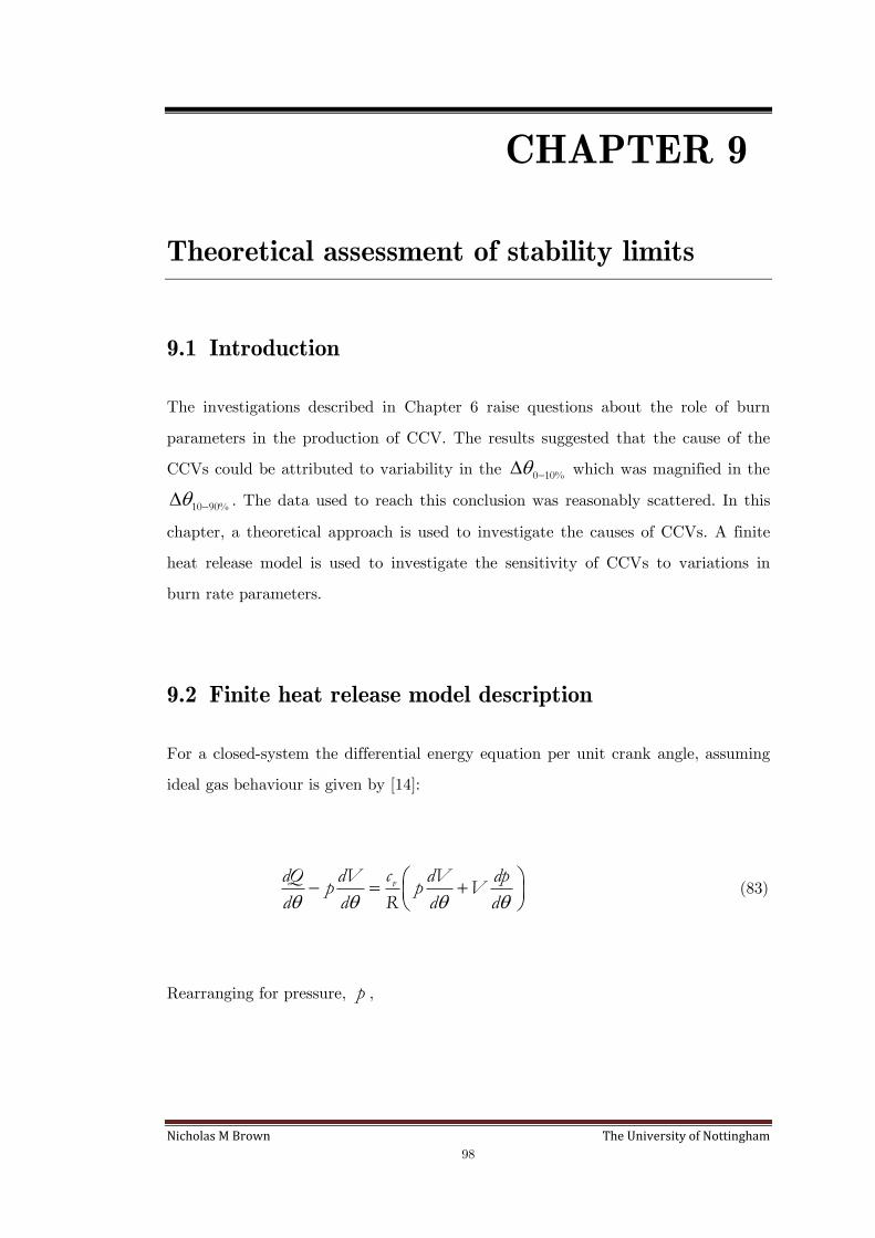
Nicholas M Brown The University of Nottingham
98
CHAPTER 9
Theoretical assessment of stability limits
9.1 Introduction
The investigations described in Chapter 6 raise questions about the role of burn
parameters in the production of CCV. The results suggested that the cause of the
CCVs could be attributed to variability in the 0 10% which was magnified in the
10 90% . The data used to reach this conclusion was reasonably scattered. In this
chapter, a theoretical approach is used to investigate the causes of CCVs. A finite
heat release model is used to investigate the sensitivity of CCVs to variations in
burn rate parameters.
9.2 Finite heat release model description
For a closed-system the differential energy equation per unit crank angle, assuming
ideal gas behaviour is given by [14]:
vdQ dV c dV dpp p V
d d R d d
(83)
Rearranging for pressure, p ,

Nicholas M Brown The University of Nottingham
99
1dp p dV dQ
d V d V d
(84)
The rate of heat release as a function of crank angle is obtained by differentiating
the cumulative heat release and is given by:
bs
dQ dxQ
d d (85)
where sQ is the total energy available at spark, determined from the mass of fuel,
and fuel lower heating value. A typical cumulative heat release, burn fraction curve
can be represented analytically by the Wiebe (although it is noted the correct
spelling of the Wiebe is actually Vibe, as discussed in [118]) function:
( ) 1 exp
n
sb
d
x a
(86)
where dq is the heat release duration (oCA), n is the Wiebe form factor and a is
the Wiebe efficiency factor. Parameters a and n are adjustable and are used to fit
experimental data, previous work has resulted with a = 5 and n = 3 [14]. sq , is
the spark timing as set in the EMS, this differs from some research [119] whereby an
ignition timing was preferred, with the ignition timing being established when the
mass fraction burned was equal to one percent. The EMS spark timing is preferred
since in spark ignition engines there is no such thing as an ignition delay, the flame
starts to propagate outward immediately following the spark discharge. Previous
experimental work [119] using a lean burn natural gas fuelled spark-ignition engine
investigated the changes in n at different operating conditions with a fixed. A
reasonable correlation between n and spark timing was established, whereby as the

Nicholas M Brown The University of Nottingham
100
spark timing was advanced n decreased indicating that as the spark timing was
advanced the combustion rate increased. Changes in manifold pressure had no effect
on the value of n . The spark timing correlation was only presented in absolute
form, spark timing relative to the optimum, MBT* or MBT was not established.
The influence of varying both a and n on the performance of a spark ignition
engine has been investigated by Caton [120] using a thermodynamic cycle
simulation. As a was increased it was shown that the start of combustion needed to
be retarded to maintain maximum performance, a similar requirement was
established when n was increased. Whereby parameters such as power and thermal
efficiency increased modestly as a was increased from 3 to 7, with the effect of a
small increase in n 1 to 3 resulting in a negligible increase.
9.3 Wiebe function investigation
The effect of changes in these parameters for a constant dq is shown in Figure 94.
Increasing a results in an almost equal decrease in both the 0 10% and the
10 90% whereas increasing n results in only an increase in the 0 10% . The
Wiebe function was fitted (minimising the sum of the square errors) to the
measured mass fraction burn curves by manipulating both a and n . The sensitivity
of a and n to different definitions of dq was investigated, whereby the dq was
varied by adopting two different end of combustion locations, when bx of the
measured data equalled 90% and 99%. Figure 95 and Figure 96 indicate that values
of a and n are insensitive to the two definitions of the dq , for this study 99% was
used to indicate the end of combustion. The average correlation coefficient (R2)
between the measured and the fitted Wiebe function was >0.99, indicating an
extremely good correlation and validating the applicability of using the function for
this investigation. The influence of previously discussed parameters, namely relative
spark timing and GFR on the values of a and n are shown in Figure 97a and b. At
MBT* a is at a maximum value, this suggests that 0 10% is at a minimum with
MBT* spark timing, this is contrary to what the experimental data had shown
previously, although the difference in the value of a would result in only a small

Nicholas M Brown The University of Nottingham
101
change in the 0 10% , approximately 1oCA. The trend for an increasing value of a
with increasing GFR again is contrary to the experimental data, whereby it has
been shown that as the GFR increases so does the 0 10% , as with the spark
timing influence the magnitude of change in a results in only small change in the
0 10% . The effect on the 10 90% as a increases is more consistent with those
trends exhibited by the experimental data for changes in relative spark timing,
whereby at MBT* the 10 90% is at the shortest duration, with increasing duration
as the spark timing is retarded. The proportional relationship between GFR and a
is again contrary to the experimental data. This raises concerns as to the validity of
using the Wiebe function for describing accurately the trends exhibited by the
experimental data, yet as can be seen there is significant scatter about the trends
established. The trends established for n reflect more those seen with the
experimental data, as the spark timing is retarded from the optimum n reduces
indicating a more rapid 0 10% , n also increases with GFR again this relationship
was also apparent in the experimental data. It should also be noted that the
experimental scatter is significantly less than that seen for a .
Although values of a and n can be adjusted to fit the experimental data, if the
combustion duration is fixed as has been used here the value of a should also be
fixed since
ln(1 0.99) 4.6052a (5)
The change in n as a function of relative spark timing and GFR is re-investigated
with the value of a set to 4.6052, the results are shown in Figure 98. Fixing
a changes the fitted values of n and more importantly the trend as GFR changes.
Where previously as GFR had increased the value of n also increased which
indicated an increase in the 0 10% which was consistent with the experimental
data, with a fixed the fitted values of n decrease, suggesting a decrease in 0 10%
with increasing GFR. The trend of a decrease in the value of n as the spark timing
is retarded is maintained. It should be noted that the performance of the fit is
Nicholas M Brown The University of Nottingham
102
degraded, as would be expected when only n is being varied but the level of
degradation is not significant, average R2 changing reducing from 0.992 to 0.9969.
Generally the results suggest the Wiebe function is not ideal in modelling
experimental burn data, particularly where the data covers a wide range of
operating conditions and of relevance to this data set, the wide range of burn
durations. Although it is not correct to vary both parameters, n and a , it has been
shown that the results from this investigation provides values, particularly of n
that are more representative of the trends shown by the experimental data. By
varying a with a fixed duration, determined from the experimental data it is in
effect introducing a method for varying the duration of the combustion. The range
of fitted a values was between 3.454 and 8.301 which is equivalent to burn
durations of 96.8% to 99.9%, this converts to no more than 6oCA increase in
combustion duration, taking this into account it could be concluded that by varying
a it allows errors in the experimentally derived burn rate to be accounted for.
9.4 Modelling methodology
A matrix of simulations was created adopting a single factorial approach. The
parameters varied were a , n , dq and spark timing Table 8 shows the range of each
parameter. The ranges encompassed values measured experimentally. Each
simulation consisted of running the model 500 times while applying random
variations to the mean value of each parameter, thus simulating CCV. The
magnitude of the randomness was increased, for example all mean parameter values
were fixed, including the variability of the parameter being investigated. Typically
three runs were conducted, with the variability increasing for subsequent runs
following the datum run, where typically the COV of the parameter resulted in
variability that was consistent with stable engine operating conditions. Figure 99
provides an example of the output from the model, whereby the correlation between
gIMEPCOV and both 0 10%COV and 10 90%
COV is shown. There is good correlation
between 0 10%COV and
gIMEPCOV , as indicated by the R2 value of 0.96,
Nicholas M Brown The University of Nottingham
103
interestingly the correlation between 10 90%COV and
gIMEPCOV is poor, suggesting
CCV are particularly sensitive to variations in the 0 10% and less so to those
associated with the 10 90% . It should be noted though, that this is only an
example of the output from the model and with a relatively fast total burn duration.
To investigate the sensitivity of CCV to the varied parameters the results
themselves were modelled using the MBC toolbox in MATLAB, the same tool that
was used to model the cylinder residual gas fraction (see Chapter 3).
9.5 Modelling results
The key parameters, 0 10%COV and 10 90%
COV were used as inputs to the model of
gIMEPCOV . The models created included only polynomial terms so as to establish
the parameters that had the greatest influence on gIMEPCOV . The polynomial order
was also limited to a maximum of six since although increasing the order would
improve the fit of the models to the data it would also mean establishing dominant
factors would become increasingly difficult. The final restriction was to only model
results that had gIMEPCOV > 5, since values below this are within expected
‘normal’ operating variability. The results from the models using 0 10%COV and
10 90%COV as the only input factors did not provide satisfactory correlations as
shown in Table 9. In an attempt to resolve the poor correlation an additional term
was added. Along with 0 10%COV and 10 90%
COV , dq was added since typically
increasing combustion variability is associated with increasing dq . Table 10 provides
the new correlation coefficients with the additional input factor. In all cases the
correlation coefficients have improved, although the 6th order model appears the best
in terms of ability to model the trends a review of all models indicated the cubic
model provided the most realistic trends.
The results of the model are presented in Figure 100. The modelled data presented
is consistent with the measured results, whereby as the dq increases the effect of
increasing 10 90%COV results in greater
gIMEPCOV . What the model does not reflect
is a correlation between 0 10%COV and 10 90%
COV that was suggested by the
Nicholas M Brown The University of Nottingham
104
measured data, in fact the model indicates maximum gIMEPCOV with minimum
0 10%COV . This is not fully unexpected,
gIMEPCOV is always going to be more
sensitive to variations in 10 90%COV since it is over this burn duration that the
largest proportion of gIMEP is produced. The investigation in this chapter has
indicated that the model used here, or particularly the model used to simulate the
burn profile does not have sufficient coupling between the 0 10% and 10 90% .
Importantly it also shows this kind of model is unlikely to provide sufficient detail
to enable such a correlation to be found.
9.6 Discussion and Summary
A finite heat release model was used to investigate the correlations between
0 10%COV and 10 90%
COV and gIMEPCOV . An investigation of the Wiebe function
indicated that by manipulating both a and n the function matched the measured
data very well, although the trends developed for a did not generally support the
experimental findings. The ability of such a simple function to predict the burn
duration of such a wide range of operating conditions indicates the validity of using
it for modelling purposes. The finite heat release model was used to investigate the
effect of random variations in the burn rate. The results indicated that increasing
variations in 10 90%COV lead to the greatest variations in
gIMEPCOV , there was no
correlation with 0 10%COV , to gain a reasonable such fit through the data dq was
required. The results indicated that although such a model can be used to
investigate influences on gIMEPCOV the ability to understand causes of CCV and
the propagation of early flame variations into later burn phases cannot be
established. Work should be focused on flame surface imaging to understand better
the transmission of early flame variability to later stages, this work along with a
CFD based modelling approach could be used to better establish a link between
variability in early flame development and whether that variation propagates and
magnifies into the rapid burning phase.
Nicholas M Brown The University of Nottingham
105
CHAPTER 10
Discussions and Conclusions
10.1 Introduction
Accurate understanding of emissions and combustion variability over a wide range
of operating conditions is key in understanding the robustness of the combustion
system. Without this knowledge issues could arise with calibration and
aftertreatment systems such as catalysts. A significant amount of research has been
focused at understanding emissions and combustion variability. The knowledge of
both has increased significantly with highly complex models providing detailed
understanding of emissions formation and the combustion process. This research is
key to providing a better understanding of both processes, but establishing stable
operating limits and functions to describe emissions based on experimental engine
data provides significant insight into the robustness of the combustion system.
This thesis focuses on developing and assessing stable operating limits for a typical
modern PFI engine with variable intake valve timing and understanding the causes
of unstable combustion. This work is presented alongside further developments of
functions describing emissions across the entire operating envelope.
10.2 Discussion
The work in this thesis develops models to describe emissions across the entire
engine operation and develops physical and chemical limits on stable combustion.
Both investigations include further work to underpin the correlations based on
theoretical approaches. The experimental work was carried out on a modern PFI SI
engine with VVTi, the addition of VVTi was shown to have a significant influence
Nicholas M Brown The University of Nottingham
106
on the residual gas fraction. It was key to the investigation to establish accurate
understanding of the residual gas fraction due to changes in valve overlap. This was
achieved by the use of in cylinder gas sampling which provided the necessary
information to calculate accurately the residual gas fraction. Although the in-
cylinder sampling provides the most accurate method of determining the residual
gas fraction NOx emissions have been shown to be highly sensitive to changes in
residual gas fraction. Changes in NOx emissions could therefore be used in the
future on engines with more complex valve timing/ phasing systems to indirectly
calculate the residual gas fraction.
The determination of mass fraction burned profiles from experimental data was
investigated thoroughly ensuring a robust method was adopted. The two commonly
used methods Rassweiler and Withrow and the approach based on the first law of
thermodynamics were evaluated. Both methods resulted in very similar initial burn
periods but there was significant variations in the rapid burn period. In the current
study, the Rassweiler and Withrow method was adopted. The differences found
raises questions as to the ability to compare researchers results since variability in
mass fraction burned will occur simply due to the calculation method.
Limits on stable combustion have been established that are defined using chemical
terms namely AFR and GFR and relative spark timing. The GFR term takes into
account variations in the residual gas fraction, which enables data to be collapsed on
to a single characteristic. Although GFR is a robust parameter for standard gasoline
operation an alternative parameter, TDP [6] has been shown to be applicable for
different fuel operation since this parameter approximates the flame temperature of
the mixture which GFR would not do. The widest range of stable operation occurs
when spark timing is set to MBT* and although a slight reduction occurs as the
spark timing is initially retarded a significant reduction occurs when the start
timing is retarded by 20degs. During normal vehicle operation the engine is unlikely
to be running at such significant spark retards due to the efficiency penalty
associated with such spark timings. Times when this spark retard maybe used is
during starting and the idle period post starting so as to achieve rapid catalyst light
off times. The implication of the findings suggest care should be taken when using
excessive spark retard since the potential for unstable combusting cycles to occur

Nicholas M Brown The University of Nottingham
107
increases significantly. The stable combustion island developed could be used as an
initial go/ no go criteria for engine calibration since it will be generically similar for
all port fuelled gasoline engines.
The limits on stable combustion was characterised using gIMEPCOV , this parameter
describes variations in work output from the engine. gIMEPCOV only provides an
understanding of variability in work output which is an integral parameter, it does
not provide an understanding of the causes of the variation. Analysis of the burn
rates and the key burn phases, the 0 10% and the 10 90% indicted that moving
towards chemical stability limits resulted in increased variability and duration in
both combustion phases. The variability in work output was manifested in the
0 10% and magnified in the 10 90% . This is consistent with results presented by
other researchers. It should be noted that although variations in the 0 10% result
in variations in 10 90% it is the variations in the latter that directly influences the
value of gIMEPCOV . Moving towards the physical stability limit by retarding the
spark timing resulted in a similar phenomenon as with the chemical limits, although
the correlation between variability in 0 10% and 10 90% reduced as the spark
timing was retarded. The reduced correlation is caused by the combustion being
phased significantly into the exhaust stroke therefore increasing the susceptibility of
the 10 90% phase to partial burning which would not be reflected in the 0 10% .
Parameters affecting emissions were evaluated, CO and HC emissions could be
described using equivalence ratio. The key to improving the accuracy of the HC
emissions predictions was to add functions that take into account valve overlap and
particularly unstable combustion. Increasing valve overlap was found to reduce HC
emissions compared to the typical timings adopted, although this improved the
predictive capability of the model, the key addition was to add HC contributions
from unstable combustion. Over the NEDC drive cycle the additional unstable term
was shown to result in significantly increased HC emissions during transient
operation, essentially caused by the wide fluctuations in AFR/ GFR during the
manoeuvres. NOx emissions were only influenced by AFR and bx , there was no
direct change in NOx emissions with valve timing. Theoretical evaluation of the
Nicholas M Brown The University of Nottingham
108
NOx function indicated the predictions were generally consistent with those from
Zeldovich formation mechanism.
10.3 Further Work
Factors affecting emissions and combustion stability have been investigated in this
thesis. Much of the work is experimental and although some theoretical assessments
have been made more work could be conducted in this area. With increased focus on
greater fuel economy and the use of different fuels to facilitate ultra lean
combustion, research in this field with reference to the work presented here could be
used to understand the benefits and limitations of different technologies.
Specific examples of areas that should be investigated further include:
Comparisons of combustion stability of stratified SI combustion systems,
does the combustion system exhibit the same characteristics in terms of
how combustion stability degrades?
Comparisons of combustion stability of direct injection compression ignition
combustion systems, again can correlations and comparisons be made
enabling more generic understanding of what limits stable combustion in
all the reciprocating engine forms?
The functions used to describe emissions for both NOx and CO were
reasonable in the level of accuracy the predictions provided. HC emissions
were more scattered. Further experimental work and modelling is
recommended to be undertaken to understand the sources of variability.
Operating the experimental engines on gaseous fuels would provide a good
basis for removing some scatter from the data.
The addition of unsteady combustion predictions in NuSIM could be coupled
with an aftertreatment model to better understand the implications of
unstable combustion events on catalyst efficiencies and therefore vehicle
out emissions.
Nicholas M Brown The University of Nottingham
109
The experimental work presented here was conducted using an instrumented V8
engine. Although this engine was ideal for this work since it provided a production
engine configuration further research work on both emissions and combustion
benefit from utilising single cylinder engines. These provide a flexible tool for
improving understanding and reducing experimental variability in terms of
emissions and combustion measurements. Single cylinder engines can also be
modified allowing optical access enabling an additional number of measurements to
be taken facilitating better understanding of the combustion process.
10.4 Conclusions
Chapter 3 – Test facility and experimental variables
AFR can be determined indirectly using sensors, such as UEGO or HEGO or
directly from the air induced and fuel injected. For unstable combustion
operating conditions significant errors in AFR occur from using the sensors.
Increasing the VO by phasing the intake valve while the exhaust valve
timing remains constant increases the rx whereby the variables, in the order
of greatest influence on rx are MAP, VO and rpm.
Chapter 4 – Mass fraction burn determination
Comparisons between the Rassweiler and Withrow approach and a heat
release model including heat transfer and blowby terms to calculate the mass
fraction burned profile indicated the rapid burn duration was greater using
the heat release approach.
The number of cycles required to establish variations in burn rates was 50
and 200 for stable and unstable operating conditions respectively.
Chapter 5 – Physical and chemical limits of stable operation
Limits of stable combustion can be defined using GFR and AFR, whereby
the rich limit is defined at a given AFR and lean limit at a constant GFR. A
non linear function of AFR and GFR describes the stability limit between
the rich and lean limit, where the most robust operating conditions are
slightly rich of stoichiometric.
Nicholas M Brown The University of Nottingham
110
Two different test methodologies were used to investigate the stability limits,
both methods, constant air and fuel resulted in the same stability limits
being establish. Indicating the parameters used are robust.
The greatest range of stable combustion occurs at MBT* spark timing, a
small decrease in the stable range occurs at dMBT*=10, where further spark
retard, dMBT*=20 results in a significant reduction.
gIMEPCOV should be used for investigating combustion variability, significant
variations in the pumping work causes nIMEPCOV to not just reflect
combustion variability.
Chapter 6 – The cause of stability limits
The flame development time decreases to a minimum as the spark timing is
retarded from MBT* (as the spark timing moves towards TDC), whereas the
rapid burn time continuously increases.
There is a reasonable correlation between the variability in the flame
development time and rapid burn time, indicating cycle to cycle variability is
predominantly caused in the flame development and magnified in the rapid
burn time.
Chapter 7 – Emissions Characterisation
CO emissions for both unstable and stable combusting conditions can be
described as only a function of equivalence ratio.
For stable combustion operation and typical valve timings and overlaps HC
emissions can be described using only equivalence ratio. Additional functions
are required to provide an accurate model of HC emissions, taking into
account valve timing, relative spark timing and combustion stability.
NOx emissions can be described using AFR, GFR and relative spark timing,
no correction for unstable combustion conditions is required.
Combustion efficiency traditionally described as a function of equivalence
ratio is also a function of burned gas fraction whereby increasing burned gas
fraction at a constant equivalence ratio reduces the combustion efficiency.
Chapter 8 – Emissions Generic Function Physical Underpinning
HC emissions can be broken down into two sources, bulk and unstable
combustion related. Under normal operation hydrocarbon emissions are
predominantly caused by unburned fuel being trapped in the crevices. The
greatest contribution though comes from unstable combustion.
Nicholas M Brown The University of Nottingham
111
NOx emissions can be described using the extended Zeldovich thermal NOx
mechanism the results are consistent with the NOx generic function
developed.
Chapter 9 – Theoretical assessment of stability limits
The Wiebe function can be used to accurately describe a wide range of
experimental data including stable and unstable combusting operating
conditions by manipulating both a and n .
A theoretical assessment of the causes of gIMEPCOV indicated 0 10%
COV ,
10 90%COV and combustion duration are the key parameters. Where
increasing 10 90%COV is the dominant factor in increasing
gIMEPCOV .
Nicholas M Brown The University of Nottingham
112
References
1. Colls, J, ‘Air Pollution’, E & FN Spon, 1997.
2. US Department of Energy: EERE (Energy Efficiency and Renewable Energy).
http://www.eere.energy.gov/vehiclesandfuels/facts/2005/fcvt_fotw386.shtml
accessed 9th of November 2005.
3. ‘Directive 98/69/EC of the European Parliament and of the Council’, Official
Journal of the European Committees, October 1998.
4. Winborn L D, ‘The Cold Operation of SI Engines and the Significance of Fuel
Losses, Oil Dilution, and Mixture Gas/Fuel Ratio’, PhD Thesis, University of
Nottingham, 2001.
5. Lai W C, ‘Valve Timing, Charge Dilution and Cycle-To-Cycle Stability of Work
Output of a Spark Ignition Engine’, PhD Thesis, University of Nottingham,
2004.
6. Tully E J, Heywood J B, ‘Lean-Burn Characteristics of a Gasoline Engine
Enriched with Hydrogen from a Plasmatron Fuel Reformer’, SAE Paper 2003-
01-0630, 2003.
7. Shayler P J, Chick J, Darnton N J, Eade D, ‘Generic Functions for Fuel
Consumption and Engine-out Emissions of HC,CO and NOx of Spark-Ignition
Engines’, Proceedings of ImechE, Part D, Journal of Automobile Engineering,
Vol 213, pp365-378, 1999.
8. Harbor N, ‘The Development and Integration of Systems Models for the
Simulation of V8 Engine Performance Attributes’, PhD Thesis, University of
Nottingham, 2004.
9. ‘Directive 98/69/EC of the European Parliament and of the Council’, Official
Journal of the European Committees, October 1998.
10. Gupta V, ‘The Modelling of Automotive Engines and Emissions Aftertreatment
to Investigate Behaviour and Control’, PhD Thesis, University of Nottingham,
2005.
11. Shiomoto G H, Sawyer R F and Kelly, ‘Characterisation of the Lean Misfire
Limit’, SAE Paper 780235, 1978.
12. Brown A G, Stone C R and Beckwith P, ‘Cycle-To-Cycle Variations in Spark
Ignition Engine Combustion – Part I: Flame Speed and Combustion
Measurements and a Simplified Turbulent Combustion Model, SAE Paper
960612, 1996.
13. Horie, K, et al, ‘The Development of a High Fuel Economy and High
Performance Four-Valve Lean Burn Engine’, SAE Paper 920455, 1992.

Nicholas M Brown The University of Nottingham
113
14. Heywood J B, ‘Internal Combustion Engine Fundamentals’, McGraw-Hill, 1988.
15. Hillard J C and Springer G S, ‘Fuel Economy in Road Vehicles Powered by
Spark Ignition Engines’, Plenum Press, New York & London, pp186, 1984.
16. Geiger J, Pischinger S, Bowing R, Kob H-J and Thiemann J, ‘Ignition Systems
for Highly Dilute Mixtures in SI-Engines’, SAE Paper 1999-01-0799, 1999.
17. Goldwitz J A and Heywood J B, ‘Combustion Optimization in a Hydrogen-
Enhanced Lean Burn SI Engine’, SAE Paper 2005-01-0251, 2005.
18. Hori T, Shibata M, Okabe S and Hashizume K, ‘Super Ignition Spark Plug with
Fine Centre & Ground Electrodes’, SAE Paper 2003-01-0404, 2003.
19. Rivin B, Dulger M and Sher E, ‘Extending Lean Misfire Limit of Methane-Air
Mixtures by Means of an Enhanced Spark Discharge’, SAE Paper 1999-01-0573,
1999.
20. Gillespie L, Lawes M, Sheppard C G W and Woolley R, ‘Aspects of Laminar
and Turbulent Burning Velocity Relevant to SI Engines’, SAE Paper 2000-01-
0192, 2000.
21. Inoue T, Matsushita S, Nakanishi K and Okano H, ‘Toyota Lean Combustion
System – The Third Generation System’, SAE Paper 930873, 1993.
22. Johansson B and Soderberg F, ‘The Effect of Valve Strategy on In-Cylinder
Flow and Combustion’, SAE Paper 960582, 1996.
23. Arcoumanis C, Bae C S and Hu Z, ‘Flow and Combustion in a Four-Valve,
Spark-Ignition Optical Engine’, SAE Paper 940475, 1994.
24. Hires S D, Tabaczynski R J and Novak J M, ‘The Prediction of Ignition Delay
and Combustion Intervals for a Homogeneous Charge Spark Ignition Engine’,
SAE Paper 780232, 1978.
25. Young M B, ‘Cyclic Dispersion – Some Quantitative Cause-and-Effect
Relationships’, SAE Paper 800459, 1980.
26. Hacohen J, Belmont M R and Ashcroft S J, ‘Flame Speed in a Spark Ignition
Engine’, SAE Paper 942050, 1994.
27. Matekunas F A, ‘Modes and Measures of Cyclic Combustion Variability’, SAE
Paper 830337, 1983.
28. Russ S, Lavoie G and Dai W, ‘SI Engine Operation with Retarded Ignition: Part
1 – Cyclic Variations’, SAE Paper 1999-01-3506, 1999.
29. Rousseau S, Lemoult B and Tazerout M, ‘Combustion characterisation of
Natural Gas in a Lean Burn-Ignition Engine’, Proceedings of ImechE, Part D,
Journal of Automobile Engineering, Vol. 213, pp481-489, 1999.
30. Johansson B, ‘Influence of the Velocity near the Spark Plug on Early Flame
Development’, SAE Paper 930481, 1993.
Nicholas M Brown The University of Nottingham
114
31. Holmstrom Karin and Denbratt I, ‘Cyclic Variations in an SI Engine Due to the
Random Motion of the Flame Kernel’, SAE Paper 961152, 1996.
32. Bradley D, Lawes M and Sheppard C G W, ‘Combustion and the
Thermodynamic Performance of Spark Ignition Engines’, Proceedings of ImechE,
Part C, Journal of Mechanical Engineering Science, Vol. 214, pp257-268, 2000.
33. Gatowski J A, Heywood J B and DeLeplace C, ‘Flame Photographs in a Spark-
Ignition Engine’, Combustion and Flame, Vol. 56, pp.71-81, 1984.
34. Kuroda H, Nakajima Y, Sugihara K, Takagi Y and Muranaka S, ‘The Fast Burn
with Heavy EGR, New Approach for Low NOx and improved Fuel Economy’,
SAE Paper 780006, 1978.
35. Harrington J, ‘A Study of Carburation Effects on Power Emissions Lean Misfire
Limit & EGR Tolerance of a Single Cylinder Engine’, SAE Paper 760754, 1976.
36. Shiomoto G H, Sawyer R F and Kelly, ‘Characterisation of the Lean Misfire
Limit’, SAE Paper 780235, 1978.
37. Quader A A, ‘Lean Combustion & The Misfire Limit in Spark Ignition Engines,
SAE Paper 741055, 1974.
38. Ryan T W, Lestz S S and Meyer W E, ‘Extension of the Lean Misfire Limit and
Reduction of Exhaust Emissions of an SI Engine by Modification of the Ignition
and Intake System’, SAE Paper 740105, 1974.
39. Hill M J, ‘The Limits and Control of Mixture Leaness for Stable Engine
Operation’, PhD Thesis, University of Nottingham, 2001.
40. Ozdor N, Dulger M and Sher E, ‘Cyclic Variability in Spark Ignition Engines: A
Literature Survey’, SAE Paper 940987, 1994.
41. Asmus T W, ‘Fuel Economy in Road Vehicles Powered by Spark Ignition
Engines’, Plenum Press, 1984, pp149-181, Editors Hillard J C and Springer G S.
42. Moriya Y, Watanabe A, Uda H, Kawamura H, Yoshioka M and Adachi, M, ‘A
Newley Developed Intelligent Variable Valve Timing System – Continuously
Controlled Cam Phasing as Applied to a New 3 Litre Inline 6 Engine’, SAE
Paper 960579, 1996.
43. Leone T G, Christenson E J and Stein R A, ‘Comparison of Variable Camshaft
Timing Strategies at Part Load’, SAE Paper 960584, 1996.
44. Duckworth R F and Barker, L, ‘A Comparative Study of Variable Camshaft
Phasing and Port Throttling for Performance and Emissions’, SAE Paper
960580, 1996.
45. Nagumo S and Hara S, ‘Study of Fuel Economy Improvement Through Control
of Intake Valve Closing Timing: Cause of Combustion Deterioration and
Improvement’, JSAE9439311, 1995.
Nicholas M Brown The University of Nottingham
115
46. Szczupak D, Brunson D, Carling J, Cooke J, Joyce M, Massey N and White C,
‘The Jaguar AJ V8 Engine’, SAE paper 970914, 1997.
47. Signal Group, ‘MaxSys 900 System Data Manual’, Issue 1.0, 1999.
48. Rai H S, Brunt M F J and Loader C P, ‘Quantification and Reduction of IMEP
Errors Resulting from Pressure Transducer Thermal Shock in an S.I. Engine’,
SAE Paper 1999-01-1329, 1999.
49. Brunt M F J and Emtage A L, ‘Evaluation of IMEP Routines and Analysis
Errors’, SAE Paper 960609, 1996.
50. Nilsson Y and Eriksson L, ‘Determining TDC Position Using Symmetry and
Other Methods’, SAE Paper 2004-01-1458, 2004.
51. Spindt R S, ‘Air-Fuel Ratios from Exhaust Gas Analysis’, SAE Paper 650494,
1965.
52. Fukui T, Tamura Y, Omori S and Saitoh S, ‘Accuracy of A/F Calculation from
Exhaust Gas Composition of SI Engine’, SAE Paper 891971, 1989.
53. Uyehara O, ‘A Method to Estimate H2 in Engine Exhaust and Factors that
Affect NOx and Particulates in Diesel Engine Exhaust, SAE Paper 910732, 1991.
54. Urban C M and Sharp C A, ‘Computing Air/Fuel Ratio from Exhaust
Composition’, ASME, Natural Gas and Alternative Fuels for Engines, ICE - Vol.
24, 1994.
55. Lynch D and Smith W, ‘Comparison of AFR Calculation Methods Using Gas
Analysis and Mass Flow Measurement’, SAE Paper 971013, 1997.
56. SAE Recommended Practice, ‘Instrumentation and Techniques for Exhaust Gas
Emissions Measurement’, SAE J254, 1984.
57. Horiba Ltd., ‘A/F Analyser MEXA-700λ Instruction Manual’, 2000.
58. Bosch, ‘Gasoline-Engine Management’, 2nd Edition, Professional Engineering
Publishing Limited, UK, 2004.
59. Toda T, Nohira H and Kobashi K, ‘Evaluation of Burned Gas Ratio (BGR) as a
Predominant Factor to NOx’, SAE Paper 760765, 1976.
60. Fallahzadeh F, Subranhmanyam J P and Babu M K G, ‘A Variable Valve
Timing Engine for the Improvement in Engine Performance and Emission
Characteristics’, SAE Paper 2000-01-1414, 2000.
61. Schirm E, De Jesus G A R and Valle R M, ‘Performance Controlling of Spark
Ignition Engine by the Variation of the Intake Valve Opening Angle’, SAE
Paper 2003-01-3720, 2003.
62. Alger L, ‘The Advantages and Control of Variable Valve Timing Under Part-
Load Operating Conditions’, PhD Thesis, University of Nottingham, 2005.

Nicholas M Brown The University of Nottingham
116
63. Fox J W, Cheng W K and Heywood J B, ‘A Model for Predicting Residual Gas
Fraction in Spark-Ignition Engines’, SAE Paper 931025, 1993.
64. Asmus T W, ‘Valve Events and Engine Operation’, SAE Paper 820749, 1982.
65. Shelby M H, Stein R A, Warren C C, ‘A New Analysis Method for Accurate
Accounting of IC Engine Pumping Work and Indicated Work’, SAE Paper 2004-
01-1262, 2004.
66. Shayler P J, Winborn L D and Hill M J, ‘The Influence of Gas / Fuel Ratio on
Combustion Stability and Misfire Limits of Spark Ignition Engine’, SAE Paper
2000-01-1208, 2000.
67. Rassweiler G M and Withrow L, ‘Motion Pictures of Engine Flame Propagation
Model of SI Engines’, SAE Journal (Trans.), Vol.42, pp185-204, 1938.
68. Shayler P J, Wiseman M W and Ma T, ‘Improving the Determination of Mass
Fraction Burnt’, SAE Paper 900351, 1990.
69. Brunt M F J, and Emtage, A, ‘Evaluation of Burn Rate Routines and Analysis
Errors’, SAE Paper 970037, 1997.
70. Brunt M F J, and Pond, C R, ‘Evaluation of Techniques for Absolute Cylinder
Pressure Correction’, SAE Paper 970036, 1997.
71. Svehla, R A, and McBride, B J, ‘Fortran IV Computer Program for Calculating
of Thermodynamic and Transport Properties of Complex Chemical Systems’,
NASA Technical Note TND-7056, NASA Lewis Research Centre, 1973.
72. Cheng W K, Hamrin D, Heywood J B, Hochgreb S, Min K and Norris M, ‘An
Overview of Hydrocarbon Emissions Mechanisms in Spark-Ignition Engines’,
SAE Paper 932708, 1993.
73. Woschni G, ‘A Universally Applicable Equation for Instantaneous Heat Transfer
Coefficient in the Internal Combustion Engine’, SAE Paper 670931, 1967.
74. Shayler P J, May S A and Ma T, ‘Heat Transfer to the Combustion Chamber
Walls in Spark Ignition Engines’, SAE Paper 950686, 1995.
75. Cheung H M and Heywood J B, ‘Evaluation of a One-Zone Burn-Rate Analysis
Procedure Using Production SI Engine Pressure Data’, SAE Paper 932749, 1993.
76. Irving R J, ‘Applications of Cylinder Pressure Transducers as Low Cost Sensors
for Diesel Engines’, PhD Thesis, The University of Nottingham, 2008.
77. Pugh G J, ‘The Analysis of Hest Release in the Investigation of Split-Main Fuel
Injection in a Diesel Engine’, PhD Thesis, The University of Nottingham, 2004.
78. Rhodes D B and Keck J C, ‘Laminar Burning Speed Measurements of Indolene-
Air-Dilutent Mixtures at High Pressures and Temperatures’ SAE Paper 850047,
1985.
Nicholas M Brown The University of Nottingham
117
79. Stone, C R, Brown A G, and Beckwith P, ‘Cycle-by-Cycle Variations in Spark
Ignition Engine Combustion – Part II: Modelling of Flame Kernel Displacements
as a Cause of Cycle-by-Cycle Variations, SAE Paper 960613, 1996.
80. Merdjani S, and Sheppard C G W, ‘Gasoline Engine Cycle Simulation Using the
Leeds Turbulent Burning Velocity Correlations’, SAE Paper 932640, 1993.
81. Elsom D M, ‘Atmospheric Pollution: A Global Problem’, Blackwell, 1992.
82. Horn G, ‘The Prediction of Fuel Economy and Pollutant Emissions to Assess
the Benefits of Direct Injection Gasoline Engines’, PhD Thesis, University of
Nottingham, 2002.
83. Siewert R M, ‘How Individual Valve Timing Events Affect Exhaust Emissions’,
SAE Paper 710609, 1971
84. Ferguson C R, Kirkpatrick A T, ‘Internal Combustion Engines’, 2nd Edition,
John Wiley & Sons, Inc., 2001.
85. Seabrook J, Nightingale C, Richardson S H, ‘The Effect of Variables on
Hydrocarbon Emissions - An Investigation with Statistical Experiment Design
and Fast Response FID Measurements’, SAE Paper 961951, 1996.
86. Shayler P J, and Chick J, ‘A Method of Predicting Brake Specific Fuel
Consumption Maps’, SAE Paper 1999-01-0556, 1999.
87. Svehla, R A, and McBride, B J, ‘Fortran IV Computer Program for Calculating
of Thermodynamic and Transport Properties of Complex Chemical Systems’,
NASA Technical Note TND-7056, NASA Lewis Research Centre, 1973.
88. Olikara, C, and Borman G L, ‘A Computer Program for Calculating Properties
of Equilibrium Combustion Products with Some Applications to I.C. Engines’,
SAE Paper 750468, 1975.
89. Newhall H K, ‘Kinetics of Engine-Generated Nitrogen Oxides and Carbon
Monoxide’, Twelfth Symposium on Combustion, pp603-613, 1969.
90. Lavoie G A, ‘Spectroscopic Measurement of Nitric Oxide in Spark Ignition
Engines’, Combustion and Flame, Vol. 15, pp97-108, 1970.
91. Johnson G L, Caretto L S, and Starkman, E S, ‘The Kinetics of CO Oxidation
in Reciprocating Engines’, paper presented at the Western States Section, The
Combustion Institute, Spring Meeting, April 1970.
92. Lee G R and Morley C, ‘Chemical Modelling of Hydrocarbon Exhaust
Emissions’, SAE Paper 941958, 1994.
93. Linna J-R, Malberg H, Bennet P J, Palmer P J, Tian T and Cheng W K,
‘Contribution of Oil Layer Mechanism to the Hydrocarbon Emissions from
Spark-Ignition Engines’, SAE Paper 972892, 1997.
Nicholas M Brown The University of Nottingham
118
94. Haidar H A and Heywood J B, ‘Combustion Chamber Deposit Effects on
Hydrocarbon Emissions from a Spark-Ignition Engine’, SAE Paper 972887.
95. Kalghatgi G T, ‘Effects on Combustion Chamber Deposits, Compression Ratio
and Combustion Chamber Design on Power and Emissions in Spark-Ignition
Engines’, SAE Paper 972886, 1997.
96. Landsberg G B, Heywood J B and Cheng W K, ‘Contribution of Liquid Fuel to
Hydrocarbon Emissions in Spark Ignition Engines’, SAE Paper 2002-02-3587.
97. Stanglmaier R H, Li J and Matthews R D, ‘The Effects of In-Cylinder Wall
Wetting Location on the HC Emissions from SI Engines’, SAE Paper 199-01-
0502.
98. Meyer R and Heywood J B, ‘Effect of Engine and Fuel Variables on Liquid Fuel
Transport into the Cylinder in Port-Injected SI Engines’, SAE Paper 1999-01-
0563.
99. LoRusso J A, Kaiser E W and Lavoie G A, ‘In-Cylinder Measurements of Wall
Layer Hydrocarbons in a Spark Ignited Engine’, Combustion Science and
Technology, Vol. 33, pp75-112, 1983.
100. Min K, Cheng W K and Heywood J B, ‘The Effects of Crevices on the
Engine-Out Hydrocarbon Emissions in SI Engines’, SAE Paper 940306, 1994.
101. Sodre J R and Yates D A, ‘An Improved Model for Spark Ignition Engine
Exhaust Hydrocarbons’, SAE Paper 971011, 1997.
102. Bignion E and Spicher U, ‘Investigation of the Influence of Top Land
Crevice Geometry on Hydrocarbon Emissions from SI Engine’, SAE Paper
982560, 1998.
103. Bian X, Prabhu S K, Yang W, Miller D L and Cernansky N P, ‘Tracer Fuel
Injection Studies on Exhaust Port Hydrocarbon Oxidation’, SAE Paper 982559,
1998.
104. Wu K-C and Hochgreb S, ‘Numerical Simulation of Post-Flame Oxidation of
Hydrocarbons in Spark Ignition Engines’, SAE Paper 970886, 1997.
105. Eng J A, Leppard W R, Najt P M and Dryer F L, ‘Experimental
Hydrocarbon Consumption Rate Correlations from a Spark Ignition Engine’,
SAE Paper 972888, 1998.
106. Eng J A, Leppard W R, Najt P M and Dryer F L, ‘The Interaction Between
Nitric Oxide and Hydrocarbon Oxidation Chemistry in a Spark Ignition Engine’,
SAE Paper 972889, 1997.
107. Wu K-C, Hochgreb S and Norris M G, ‘Chemical Kinetic Modelling of
Exhaust Hydrocarbon Oxidation’, Combustion and Flame, Vol.25, pp193-201,
1994.
Nicholas M Brown The University of Nottingham
119
108. Drobot K, Cheng W K, Trinker F H, Kaiser E W, Siegel W O, Cotton D F
and Underwood J, ‘Hydrocarbon Oxidation in the Exhaust Port and Runner of a
Spark Ignition Engine’, Combustion and Flame, Vol.25, pp422-430, 1994.
109. Norris M G and Hochgreb S, ‘Extent of Oxidation of Hydrocarbons
Desorbing from the Lubricant Oil in Spark Ignition Engines’, SAE Paper
960069, 1996.
110. Caton J A, Heywood J B and Mendillo J V, ‘Hydrocarbon Oxidation in a
Spark Ignition Engine Exhaust Port’, Combustion Science and Technology,
Vol.37, pp153-169, 1984.
111. Quader A A, ‘Why Intake Charge Dilution Decreases Nitric Oxide Emission
from Spark Ignition Engines’, SAE Paper 710009, 1971.
112. Benson J D and Stebar R F, ‘Effects of Charge Dilution on Nitric Oxide
Emission from a Single-Cylinder Engine’, SAE Paper 710008, 1971.
113. Caton J A, ‘Detailed Results for Nitric Oxide Emissions as Determined from
a Multiple-Zone Cycle Simulation for a Spark-Ignition Engine’, ASME, ICE-Vol.
39, ICEF2002-491, 2002.
114. Dean A M and Bozzelli, ‘Combustion Chemistry of Nitrogen’, in Gas-Phase
Combustion Chemistry, ed. W C Gardiner, Jr., pp. 361-422, Springer-Verlag,
2000.
115. Rublewski M and Heywood J B, ‘Modelling NO Formation in Spark Ignition
Engines with a Layered Adiabatic Core and Combustion Inefficiency Routine’,
SAE Paper 2001-01-1011, 2001.
116. Miller R, Russ S, Weaver C, Kaiser E, Newman C, Davis G and Lavoie G,
‘Comparison of Analytically and Experimentally Obtained Residual Fractions
and NOx Emissions in Spark-Ignited Engines’, SAE Paper 982562, 1998.
117. Miller R, Davis G, Lavoie C, Newman C and Gardner T, ‘A Super-Extended
Zel’dovich Mechanism for NOx Modelling and Engine Calibration’, SAE Paper
980781, 1998.
118. Oppenheim, A K, and Kuhl, A L, ‘Life of Fuel in Engine Cylinder’, SAE
Paper 980780, 1998.
119. Rousseau, S, Lemoult, B and Tazerout, M, ‘Combustion Characterisation of
Natural Gas in a Lean Burn Spark-Ignition Engine’, Proceedings of ImechE,
Part D, Journal of Automobile Engineering, Vol 213, pp481-489, 1999.
120. Caton, J A, ‘The Effect of Burn Rate Parameters on The Operating
Attributes of a Spark-Ignition Engine As Determined From The Second Law of
Thermodynamics’, 2000 Spring Engine Technology Conference of the ASME-
ICED, 2000.
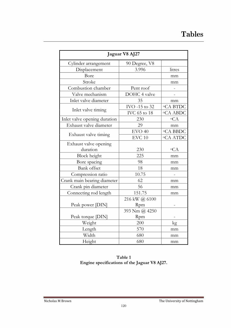
Nicholas M Brown The University of Nottingham
120
Tables
Jaguar V8 AJ27
Cylinder arrangement 90 Degree, V8
Displacement 3.996 litres
Bore mm
Stroke mm
Combustion chamber Pent roof -
Valve mechanism DOHC 4 valve -
Inlet valve diameter 35 mm
Inlet valve timing IVO -15 to 32 oCA BTDC
IVC 65 to 18 oCA ABDC
Inlet valve opening duration 230 oCA
Exhaust valve diameter 29 mm
Exhaust valve timing EVO 40 oCA BBDC
EVC 10 oCA ATDC
Exhaust valve opening duration 230 oCA
Block height 225 mm
Bore spacing 98 mm
Bank offset 18 mm
Compression ratio 10.75 -
Crank main bearing diameter 62 mm
Crank pin diameter 56 mm
Connecting rod length 151.75 mm
Peak power [DIN] 216 kW @ 6100
Rpm -
Peak torque [DIN] 393 Nm @ 4250
Rpm -
Weight 200 kg
Length 570 mm
Width 680 mm
Height 680 mm
Table 1 Engine specifications of the Jaguar V8 AJ27.
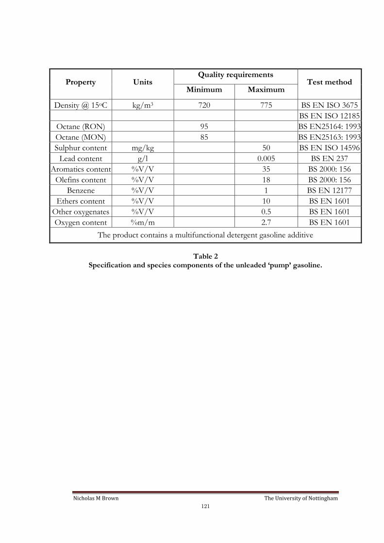
Nicholas M Brown The University of Nottingham
121
Property Units Quality requirements
Test method Minimum Maximum
Density @ 15oC kg/m3 720 775 BS EN ISO 3675
BS EN ISO 12185
Octane (RON) 95 BS EN25164: 1993
Octane (MON) 85 BS EN25163: 1993
Sulphur content mg/kg 50 BS EN ISO 14596
Lead content g/l 0.005 BS EN 237
Aromatics content %V/V 35 BS 2000: 156
Olefins content %V/V 18 BS 2000: 156
Benzene %V/V 1 BS EN 12177
Ethers content %V/V 10 BS EN 1601
Other oxygenates %V/V 0.5 BS EN 1601
Oxygen content %m/m 2.7 BS EN 1601
The product contains a multifunctional detergent gasoline additive
Table 2
Specification and species components of the unleaded ‘pump’ gasoline.
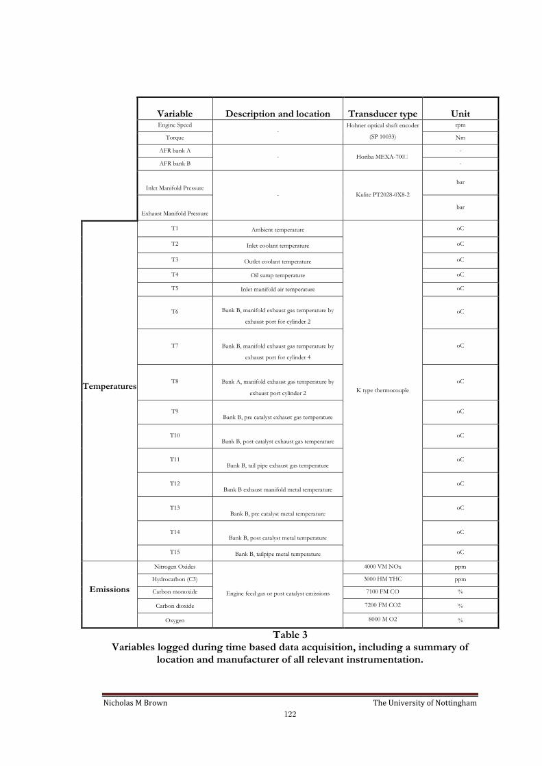
Nicholas M Brown The University of Nottingham
122
Variable Description and location Transducer type Unit
Engine Speed -
Hohner optical shaft encoder
(SP 10033)
rpm
Torque Nm
AFR bank A - Horiba MEXA-700
-
AFR bank B -
Inlet Manifold Pressure - Kulite PT2028-0X8-2
bar
Exhaust Manifold Pressure bar
Temperatures
T1 Ambient temperature
K type thermocouple
oC
T2 Inlet coolant temperature oC
T3 Outlet coolant temperature oC
T4 Oil sump temperature oC
T5 Inlet manifold air temperature oC
T6 Bank B, manifold exhaust gas temperature by
exhaust port for cylinder 2
oC
T7 Bank B, manifold exhaust gas temperature by
exhaust port for cylinder 4
oC
T8 Bank A, manifold exhaust gas temperature by
exhaust port cylinder 2
oC
T9 Bank B, pre catalyst exhaust gas temperature
oC
T10 Bank B, post catalyst exhaust gas temperature
oC
T11 Bank B, tail pipe exhaust gas temperature
oC
T12 Bank B exhaust manifold metal temperature
oC
T13 Bank B, pre catalyst metal temperature
oC
T14 Bank B, post catalyst metal temperature
oC
T15 Bank B, tailpipe metal temperature oC
Emissions
Nitrogen Oxides
Engine feed gas or post catalyst emissions
4000 VM NOx ppm
Hydrocarbon (C3) 3000 HM THC ppm
Carbon monoxide 7100 FM CO %
Carbon dioxide 7200 FM CO2 %
Oxygen 8000 M O2 %
Table 3 Variables logged during time based data acquisition, including a summary of
location and manufacturer of all relevant instrumentation.
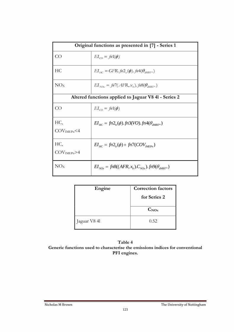
Nicholas M Brown The University of Nottingham
123
Original functions as presented in [7] - Series 1
CO 1( )COEI fn
HC *. 2 ( ). 4( )HC a dMBTEI GFR fn fn
NOX *7( , ). 8( )NOx b dMBTEI fn AFR x fn
Altered functions applied to Jaguar V8 4l - Series 2
CO 1( )COEI fn
HC,
COVIMEPn<4
*2 ( ). 3( ). 4( ) HC b dMBTEI fn fn VO fn
HC,
COVIMEPn>4
2 ( ) 7( ) HC b IMEPnEI fn fn COV
NOX *8(( , ). ). 9( )NOx b NOx dMBTEI fn AFR x C fn
Engine Correction factors
for Series 2
CNOx
Jaguar V8 4l 0.52
Table 4 Generic functions used to characterise the emissions indices for conventional
PFI engines.

Nicholas M Brown The University of Nottingham
124
GENERIC EQUATION
CO 1
21 ( ) exp( ) afn a b
21 ( ) exp( ) bfn a b c
1
1 ( )cfn a b
HC
COVIMEPn<4
& 22 ( )a b
cfn a b
23( ) . . fn VO a bVO cVO
0DMBT
4 ( ) 1 a DMBTfn
0DMBT
24 ( ) 1 5( ) 6( ). b DMBT DMBTfn fn fn EGR
25( )
b
fn a c
26( ) . . fn EGR a b EGR c EGR
HC
COVIMEPn>4
COV<4
&2 ( ) 7( )a b IMEPnfn fn COV
7( ) *IMEPn IMEPnfn COV a COV b
NOX
2x=0.13
0.112
. .8( , ) exp
x or y1 . .
b
b y
xa c AFR e AFRfn AFR x
b AFR d AFR
20DMBT
29( ) . . DMBT DMBT DMBTfn a b c
20DMBT
9( ) 0.12 DMBTfn
Altered function as used by Horn [82] and on the AJ27 engine. x is the original value for fn7, y is the altered value fitted to AJ27 engine.
Table 5 Functional form of the generic equations.

Nicholas M Brown The University of Nottingham
125
a b c d e
1 ( )afn -8.395 5.5181
1 ( )bfn -2.725 2.78 0.015
1 ( )cfn -2.725 2.78
2 ( )afn -0.00484 0.004326 0.0013313
2 ( )bfn -0.07083 0.062996 0.0232
3( )fn VO 1.072 -0.00299 -0.000127
4 ( )a DMBTfn
4 ( )b DMBTfn
5( )fn -0.00326 2.134e-4 0.0016489
6( )fn EGR 1 -0.016643 -0.002866
7( )IMEPnfn COV 0.1266 0.6728
8( , )bfn AFR x -0.00326 -0.12489 -7.41e-5 0.004 4.072e-5
9( )DMBTfn 1 -0.021 -0.00051
9( )
DMBTfn 1 -0.0505 0.00041
Function remains in the same form but the constants were altered so as to predict experimental results more accurately (Jaguar V8 4l only).
Table 6 Values of required constants used in the generic equations.
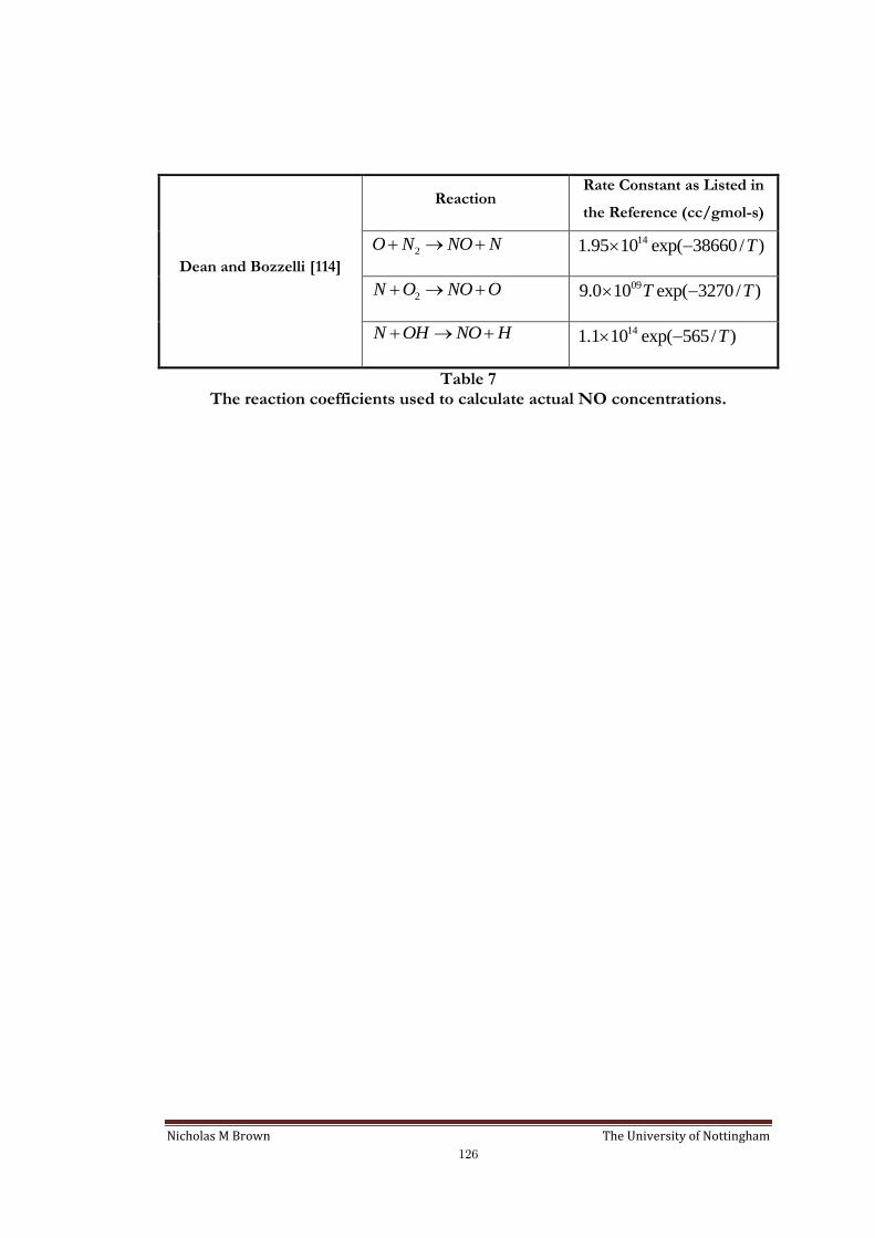
Nicholas M Brown The University of Nottingham
126
Dean and Bozzelli [114]
Reaction Rate Constant as Listed in
the Reference (cc/gmol-s)
2O N NO N 141.95 10 exp( 38660/ )T
2N O NO O 099.0 10 exp( 3270/ )T T
N OH NO H 141.1 10 exp( 565/ )T
Table 7 The reaction coefficients used to calculate actual NO concentrations.
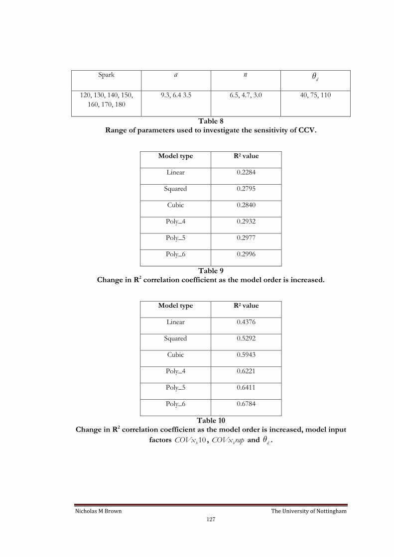
Nicholas M Brown The University of Nottingham
127
Spark a n dq
120, 130, 140, 150,
160, 170, 180
9.3, 6.4 3.5 6.5, 4.7, 3.0 40, 75, 110
Table 8 Range of parameters used to investigate the sensitivity of CCV.
Model type R2 value
Linear 0.2284
Squared 0.2795
Cubic 0.2840
Poly_4 0.2932
Poly_5 0.2977
Poly_6 0.2996
Table 9 Change in R2 correlation coefficient as the model order is increased.
Model type R2 value
Linear 0.4376
Squared 0.5292
Cubic 0.5943
Poly_4 0.6221
Poly_5 0.6411
Poly_6 0.6784
Table 10 Change in R2 correlation coefficient as the model order is increased, model input
factors 10bCOVx , bCOVx rap and dq .
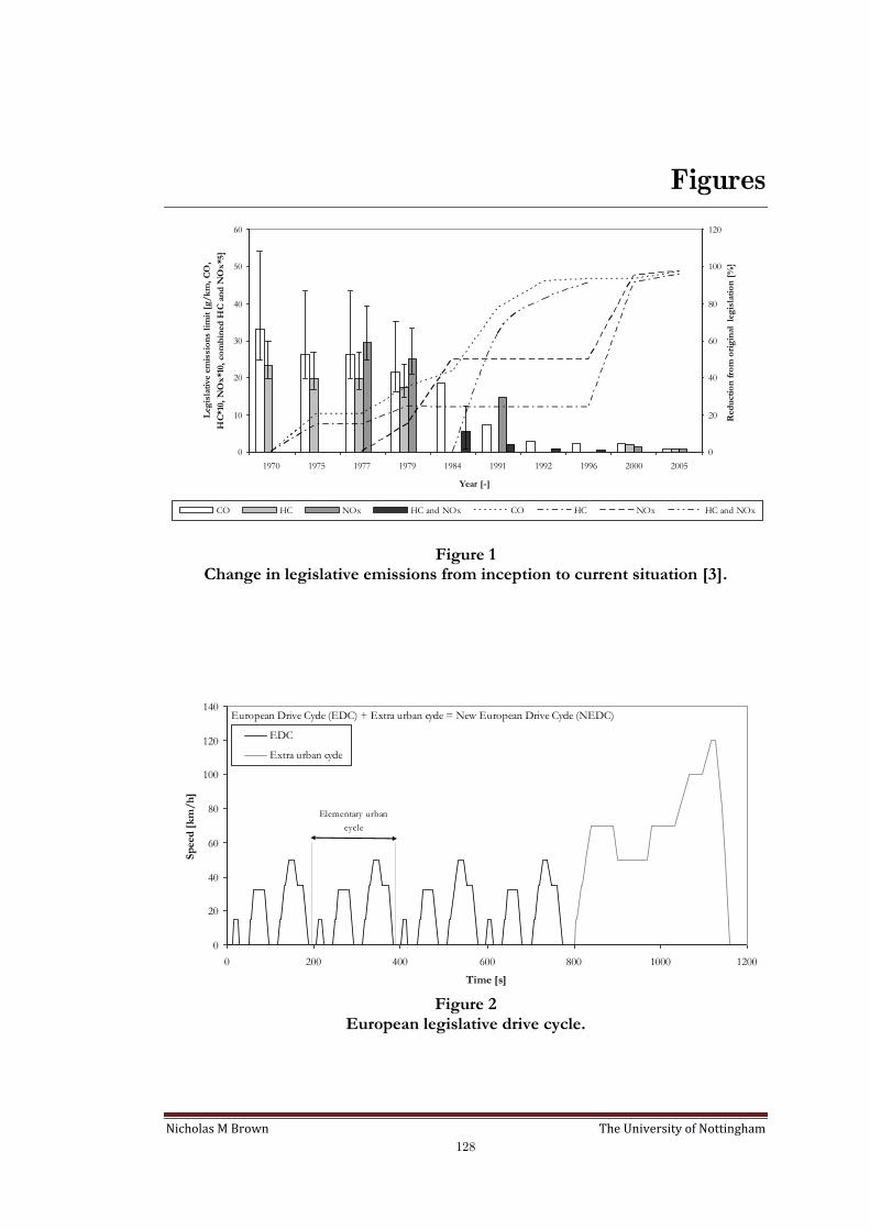
Nicholas M Brown The University of Nottingham
128
Figures
0
10
20
30
40
50
60
1970 1975 1977 1979 1984 1991 1992 1996 2000 2005
Year [-]
Leg
isla
tive
em
issi
on
s li
mit
[g
/k
m,
CO
,..
.
HC
*10,
NO
x*1
0, c
om
bin
ed H
C a
nd
NO
x*5
]..
..
0
20
40
60
80
100
120
Red
uct
ion
fro
m o
rig
inal..
. le
gis
lati
on
[%
]...
CO HC NOx HC and NOx CO HC NOx HC and NOx
Figure 1 Change in legislative emissions from inception to current situation [3].
0
20
40
60
80
100
120
140
0 200 400 600 800 1000 1200
Time [s]
Sp
eed
[k
m/
h]
EDC
Extra urban cycle
Elementary urban
cycle
European Drive Cycle (EDC) + Extra urban cycle = New European Drive Cycle (NEDC)
Figure 2
European legislative drive cycle.

Nicholas M Brown The University of Nottingham
129
TDC
IVO
BDC
EVC
10
4018
32
IVC
IVCEVO
IVO
TDC
BDC
EVC
10
4065
15
Figure 3 Minimum and maximum intake cam settings showing the associated intake
valve timing changes.
0.28
0.29
0.30
0.31
0.32
0.33
0.34
0.35
-3 -2.5 -2 -1.5 -1 -0.5 0 0.5 1 1.5 2 2.5 3
Cank angle [o]
Vo
ltag
e [
V]
2200rpm
1500rpm
idle
TDC output
Figure 4 Comparison of the output of the AVL 428 capacitance probe and the shaft encoder TDC position, the standard deviation of TDC position over the
speed range is ±0.1oCA, with an average offset from the shaft encoder TDC of ±0.4oCA.
EVO

Nicholas M Brown The University of Nottingham
130
0
5
10
15
20
25
-140 -120 -100 -80 -60 -40 -20 0 20 40 60 80 100 120 140
Crank angle [o]
Cyli
nd
er
pre
ssu
re [
bar].
spark at -50oCA,
80% of peak torque
spark at -10oCA,
10% of peak torqueMBT* spark timing
spark at 30oCA,
peak torque (24Nm)
Figure 5 In cylinder pressure traces (ensemble averaged from 500 cycles at each spark
timing). AJ27 operating at 1500rpm, light load, AFR = 14.6.
0
20
40
60
80
100
120
140
160
180
200
-40 -35 -30 -25 -20 -15 -10 -5 0 5 10
Crank angle [oATDC]
To
rqu
e [
Nm
]
Spark timing
for MBT
Spark timing
for MBT*
Figure 6 Change in brake torque with spark advance at 5 loads (0.41, 0.50, 0.57, 0.65
and 0.74 bar inlet manifold pressure) all at 1500rpm.
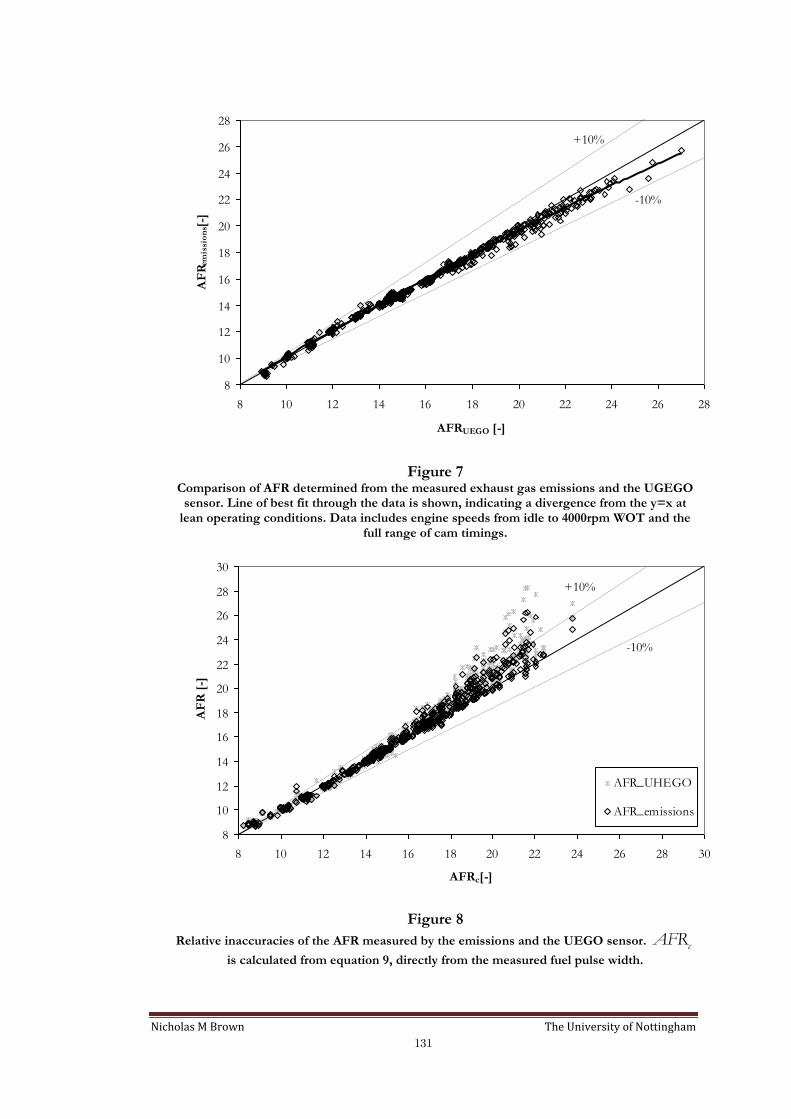
Nicholas M Brown The University of Nottingham
131
8
10
12
14
16
18
20
22
24
26
28
8 10 12 14 16 18 20 22 24 26 28
AFRUEGO [-]
AF
Rem
issi
on
s [-]
+10%
-10%
Figure 7 Comparison of AFR determined from the measured exhaust gas emissions and the UGEGO
sensor. Line of best fit through the data is shown, indicating a divergence from the y=x at lean operating conditions. Data includes engine speeds from idle to 4000rpm WOT and the
full range of cam timings.
8
10
12
14
16
18
20
22
24
26
28
30
8 10 12 14 16 18 20 22 24 26 28 30
AFRc[-]
AF
R [
-]
AFR_UHEGO
AFR_emissions
+10%
-10%
Figure 8
Relative inaccuracies of the AFR measured by the emissions and the UEGO sensor. cAFR
is calculated from equation 9, directly from the measured fuel pulse width.
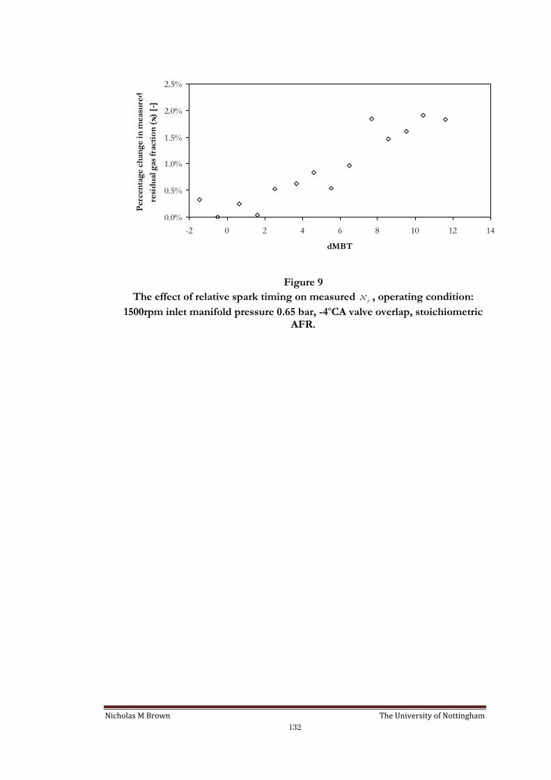
Nicholas M Brown The University of Nottingham
132
0.0%
0.5%
1.0%
1.5%
2.0%
2.5%
-2 0 2 4 6 8 10 12 14
dMBT
Per
cen
tag
e c
han
ge i
n m
easu
red.....
resi
du
al g
as
fracti
on
(x
r) [
-]..
Figure 9
The effect of relative spark timing on measured rx , operating condition:
1500rpm inlet manifold pressure 0.65 bar, -4oCA valve overlap, stoichiometric AFR.

Nicholas M Brown The University of Nottingham
133
0.00
0.05
0.10
0.15
0.20
0.25
0.30
-5 0 5 10 15 20 25 30 35 40 45
Valve overlap [oCA]
Mea
sure
d x
r [-
]...
0.48
0.75
1.00
0.00
0.05
0.10
0.15
0.20
0.25
0.30
-5 0 5 10 15 20 25 30 35 40 45
Valve overlap [oCA]
Mea
sure
d x
r [-]
...
0.43
0.68
0.95
0.00
0.05
0.10
0.15
0.20
0.25
0.30
-5 0 5 10 15 20 25 30 35 40 45
Valve overlap [oCA]
Mea
sure
d x
r [-
]...
0.40
0.66
0.93
Figure 10 The effect of valve overlap (defined as the angle at which the intake valve
opens in oCA to the oCA the exhaust valve closes, no minimum opening height applies) at three engine speeds: [a] 650rpm, [b] 1500rpm and [c] 2500rpm. The
legend in all cases is inlet manifold pressure [bar].
[a]
[b]
[c]
increasing load
increasing load
increasing load
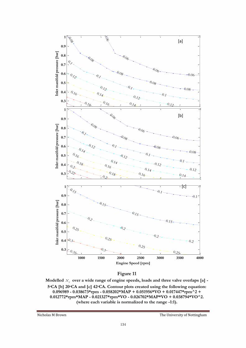
Nicholas M Brown The University of Nottingham
134
0.06
0.06
0.060.06
0.08
0.08
0.08
0.08
0.08
0.1
0.1
0.1
0.1
0.12
0.12
0.12
0.12
0.14
0.14
0.16
0.16
0.18
Inle
t m
anif
old
pre
ssu
re [
bar
]
0.3
0.4
0.5
0.6
0.7
0.8
0.9
1
0.06
0.06
0.06
0.08
0.08
0.080.08
0.1
0.1
0.1
0.1
0.12
0.12
0.12
0.12
0.14
0.14
0.14
0.140.16
0.16
0.16
0.18
0.18
0.2
0.20.22
Inle
t m
anif
old
pre
ssu
re [
bar
]
0.3
0.4
0.5
0.6
0.7
0.8
0.9
1
0.1
0.1
0.15
0.15
0.15
0.150.2
0.2
0.2
0.2
0.25
0.25
0.25
0.25
0.3
0.3
0.35
Engine Speed [rpm]
Inle
t m
anif
old
pre
ssu
re [
bar
]
1000 1500 2000 2500 3000 3500 4000
0.3
0.4
0.5
0.6
0.7
0.8
0.9
1
Figure 11
Modelled rx over a wide range of engine speeds, loads and three valve overlaps [a] -
5oCA [b] 20oCA and [c] 42oCA. Contour plots created using the following equation: 0.096989 - 0.038673*rpm - 0.058202*MAP + 0.051956*VO + 0.017447*rpm^2 +
0.012772*rpm*MAP - 0.021327*rpm*VO - 0.026702*MAP*VO + 0.038794*VO^2. (where each variable is normalized to the range -1:1).
[a]
[b]
[c]

Nicholas M Brown The University of Nottingham
135
0.8
1.0
1.2
1.4
1.6
1.8
2.0
2.2
-5 0 5 10 15 20
Valve overlap [oCA]
Measu
red
/p
red
icte
d e
q(2
4)
x
r [-
]...
0.48
0.75
1.00
0.8
1.0
1.2
1.4
1.6
1.8
2.0
2.2
-5 0 5 10 15 20 25 30 35 40 45
Valve overlap [oCA]
Measu
red
/p
red
icte
d e
q(2
4)
x
r [-
]...
0.43
0.68
0.95
0.8
1.0
1.2
1.4
1.6
1.8
2.0
2.2
-5 0 5 10 15 20 25 30 35 40 45
Valve overlap [oCA]
Measu
red
/p
red
icte
d e
q(2
4)
x
r [-
]...
0.40
0.66
0.93
Figure 12
The error ratio of measured and predicted rx at three engine speeds
(measured data as shown in Figure 11) [a] 650rpm, [b] 1500rpm and [c] 2500rpm.
[a]
[b]
[c]
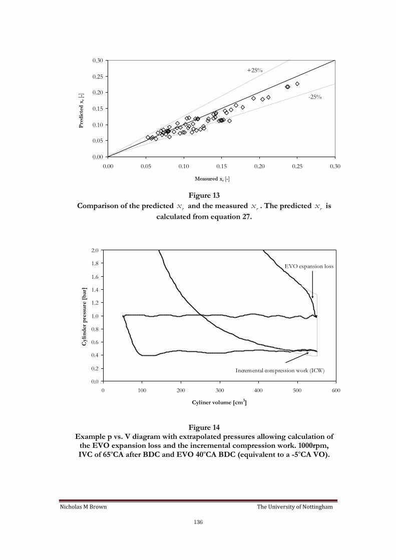
Nicholas M Brown The University of Nottingham
136
0.00
0.05
0.10
0.15
0.20
0.25
0.30
0.00 0.05 0.10 0.15 0.20 0.25 0.30
Measured xr [-]
Pre
dic
ted
xr
[-]...
+25%
-25%
Figure 13
Comparison of the predicted rx and the measured rx . The predicted rx is
calculated from equation 27.
0.0
0.2
0.4
0.6
0.8
1.0
1.2
1.4
1.6
1.8
2.0
0 100 200 300 400 500 600
Cyliner volume [cm3]
Cyli
nd
er
pre
ssu
re [
bar]....
EVO expansion loss
Incremental compression work (ICW)
Figure 14 Example p vs. V diagram with extrapolated pressures allowing calculation of
the EVO expansion loss and the incremental compression work. 1000rpm, IVC of 65oCA after BDC and EVO 40oCA BDC (equivalent to a -5oCA VO).
Measured xr [-]
Pre
dic
ted x
r [-]
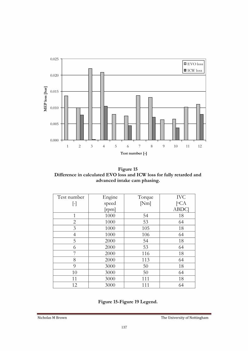
Nicholas M Brown The University of Nottingham
137
0.000
0.005
0.010
0.015
0.020
0.025
1 2 3 4 5 6 7 8 9 10 11 12
Test number [-]
ME
P lo
ss [
bar]
EVO loss
ICW loss
Figure 15 Difference in calculated EVO loss and ICW loss for fully retarded and
advanced intake cam phasing.
Test number [-]
Engine speed [rpm]
Torque [Nm]
IVC [oCA
ABDC]
1 1000 54 18
2 1000 53 64
3 1000 105 18
4 1000 106 64
5 2000 54 18
6 2000 53 64
7 2000 116 18
8 2000 113 64
9 3000 50 18
10 3000 50 64
11 3000 111 18
12 3000 111 64
Figure 15-Figure 19 Legend.
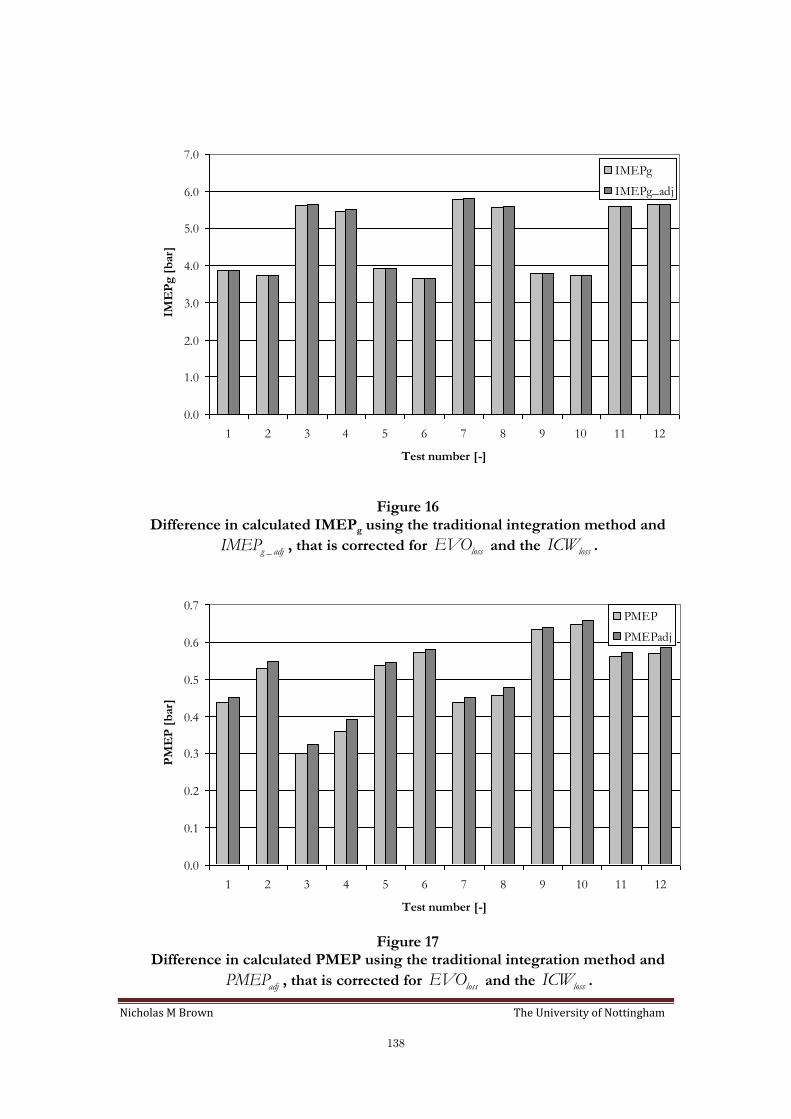
Nicholas M Brown The University of Nottingham
138
0.0
1.0
2.0
3.0
4.0
5.0
6.0
7.0
1 2 3 4 5 6 7 8 9 10 11 12
Test number [-]
IME
Pg
[b
ar]
IMEPg
IMEPg_adj
Figure 16 Difference in calculated IMEPg using the traditional integration method and
_g adjIMEP , that is corrected for lossEVO and the lossICW .
0.0
0.1
0.2
0.3
0.4
0.5
0.6
0.7
1 2 3 4 5 6 7 8 9 10 11 12
Test number [-]
PM
EP
[b
ar]
PMEP
PMEPadj
Figure 17
Difference in calculated PMEP using the traditional integration method and
adjPMEP , that is corrected for lossEVO and the lossICW .
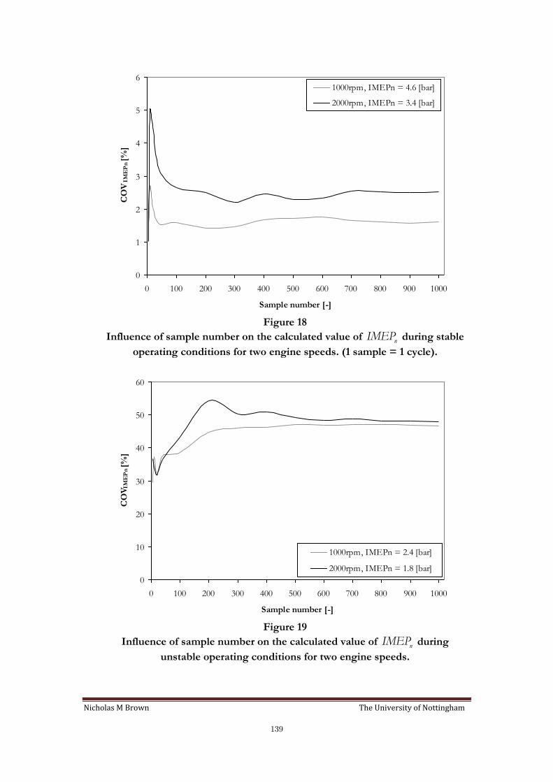
Nicholas M Brown The University of Nottingham
139
0
1
2
3
4
5
6
0 100 200 300 400 500 600 700 800 900 1000
Sample number [-]
CO
V IM
EP
n [%
]
1000rpm, IMEPn = 4.6 [bar]
2000rpm, IMEPn = 3.4 [bar]
Figure 18
Influence of sample number on the calculated value of nIMEP during stable
operating conditions for two engine speeds. (1 sample = 1 cycle).
0
10
20
30
40
50
60
0 100 200 300 400 500 600 700 800 900 1000
Sample number [-]
CO
VIM
EP
n [%
]
1000rpm, IMEPn = 2.4 [bar]
2000rpm, IMEPn = 1.8 [bar]
Figure 19
Influence of sample number on the calculated value of nIMEP during
unstable operating conditions for two engine speeds.

Nicholas M Brown The University of Nottingham
140
1.22
1.24
1.26
1.28
1.30
1.32
1.34
1.36
1.38
1.40
1.42
-45 -40 -35 -30 -25 -20 -15 -10 -5 0
Spark timing [oATDC]
Co
mp
ress
ion
po
lytr
op
ic i
nd
ex
[-]...
1000rpm
1500rpm
2000rpm
Figure 20
Influence of spark timing on calculated compression polytropic index ( )compn for
three engine speeds (constant throttle angle and valve overlap (VO) for each engine speed).
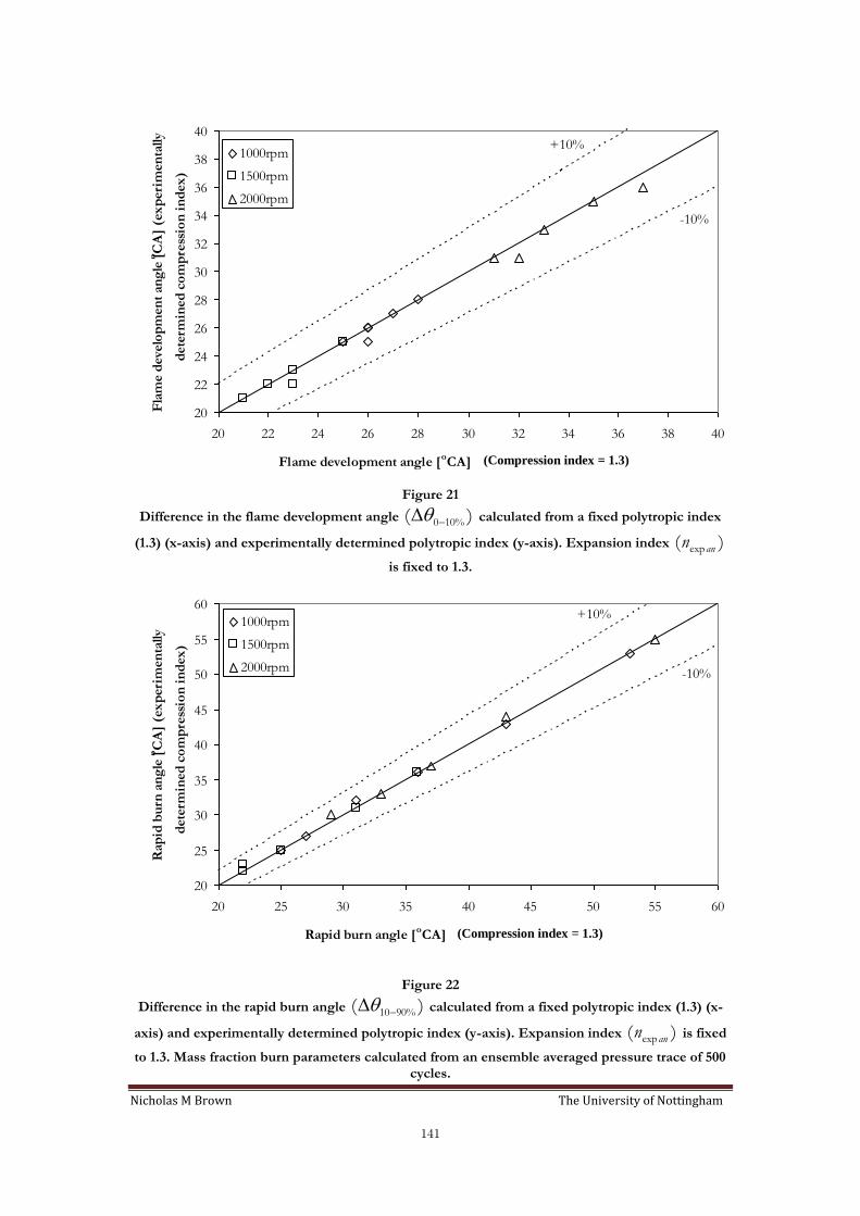
Nicholas M Brown The University of Nottingham
141
20
22
24
26
28
30
32
34
36
38
40
20 22 24 26 28 30 32 34 36 38 40
Flame development angle [oCA] (adiabatic compression index)
Fla
me d
eve
lop
men
t an
gle
[oC
A]
(ex
peri
men
tally..
dete
rmin
ed
co
mp
ress
ion
in
dex
)
1000rpm
1500rpm
2000rpm
+10%
-10%
Figure 21
Difference in the flame development angle 0 10%( ) calculated from a fixed polytropic index
(1.3) (x-axis) and experimentally determined polytropic index (y-axis). Expansion index exp( )ann
is fixed to 1.3.
20
25
30
35
40
45
50
55
60
20 25 30 35 40 45 50 55 60
Rapid burn angle [oCA] (adiabatic compression index)
Rap
id b
urn
an
gle
[oC
A]
(ex
peri
men
tally..
dete
rmin
ed
co
mp
ress
ion
in
dex
)
1000rpm
1500rpm
2000rpm
+10%
-10%
Figure 22
Difference in the rapid burn angle 10 90%( ) calculated from a fixed polytropic index (1.3) (x-
axis) and experimentally determined polytropic index (y-axis). Expansion index exp( )ann is fixed
to 1.3. Mass fraction burn parameters calculated from an ensemble averaged pressure trace of 500 cycles.
(Compression index = 1.3)
(Compression index = 1.3)
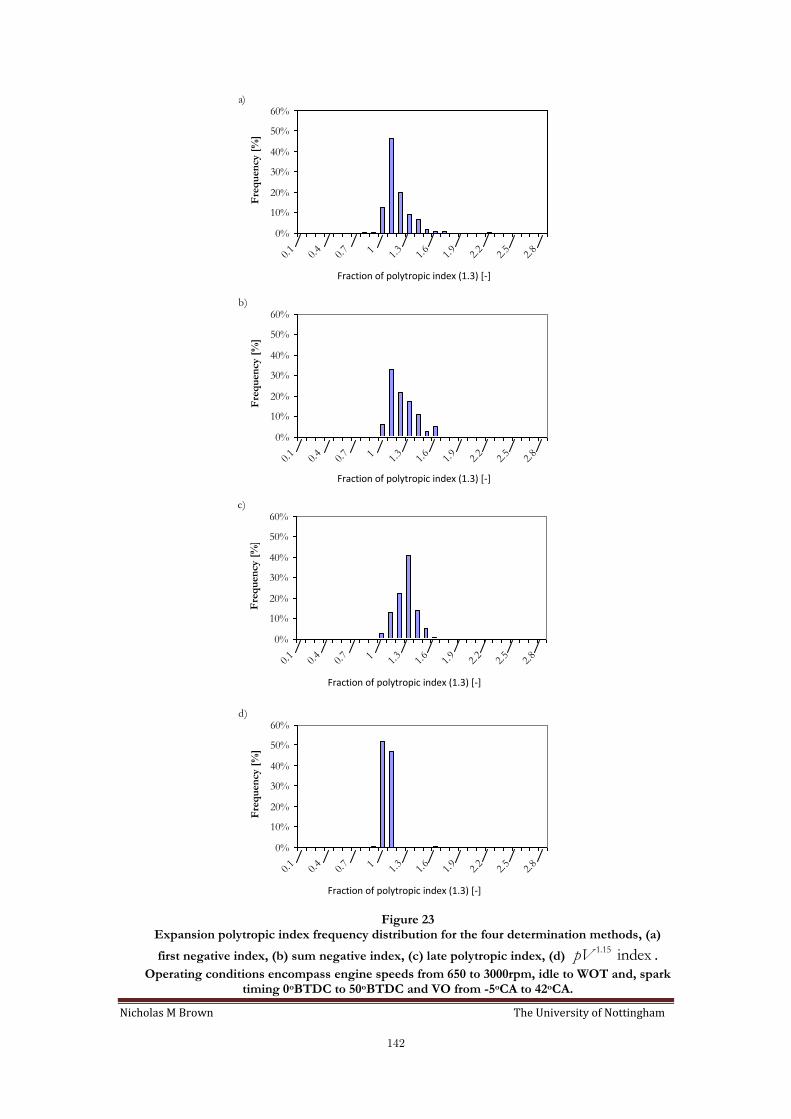
Nicholas M Brown The University of Nottingham
142
0%
10%
20%
30%
40%
50%
60%
0.1
0.4
0.7 1 1.
31.
61.
92.
22.
52.
8
Fraction of adiabatic index [-]
Fre
qu
ency
[%
]
a)
0%
10%
20%
30%
40%
50%
60%
0.1
0.4
0.7 1 1.
31.
61.
92.
22.
52.
8
Fraction of the adiabtic index [-]
Fre
qu
ency
[%
]
b)
0%
10%
20%
30%
40%
50%
60%
0.1
0.4
0.7 1 1.
31.
61.
92.
22.
52.
8
Fraction of adiabatic index [-]
Fre
qu
ency
[%
]
c)
0%
10%
20%
30%
40%
50%
60%
0.1
0.4
0.7 1 1.
31.
61.
92.
22.
52.
8
Fraction of the adiabatic index [-]
Fre
qu
ency
[%
]
d)
Figure 23 Expansion polytropic index frequency distribution for the four determination methods, (a)
first negative index, (b) sum negative index, (c) late polytropic index, (d) 1.15 indexpV .
Operating conditions encompass engine speeds from 650 to 3000rpm, idle to WOT and, spark timing 0oBTDC to 50oBTDC and VO from -5oCA to 42oCA.
Fraction of polytropic index (1.3) [-]
Fraction of polytropic index (1.3) [-]
Fraction of polytropic index (1.3) [-]
Fraction of polytropic index (1.3) [-]

Nicholas M Brown The University of Nottingham
143
20
22
24
26
28
30
32
34
36
38
40
20 22 24 26 28 30 32 34 36 38 40
Flame development angle [oCA] (adiabatic expansion index)
Fla
me d
eve
lop
men
t an
gle
[oC
A]
(ex
peri
men
tally..
dete
rmin
ed
ex
pan
sio
n i
nd
ex
)
first negative
sum negative
tuned
pV^1.15
+10%
-10%
Figure 24
Difference in the flame development angle 0 10%( ) calculated from a fixed polytropic index
(1.3) (x-axis) and experimentally determined polytropic index (y-axis). Compression index ( )compn
is fixed to 1.3. 1000rpm set of data from Figure 21.
20
30
40
50
60
70
80
20 30 40 50 60 70 80
Rapid burn angle [oCA] (adiabatic expansion index)
Rap
id b
urn
an
gle
[oC
A]
(ex
peri
men
tally..
dete
rmin
ed
ex
pan
sio
n i
nd
ex
)
first negative
sum negative
tuned
pV^1.15
+10%
-10%
Figure 25
Difference in the rapid burn angle 10 90%( ) calculated from a fixed polytropic index (1.3) (x-
axis) and experimentally determined polytropic index (y-axis). Compression index ( )compn is fixed
to 1.3. 1000rpm set of data from Figure 22.
(Expansion index = 1.3)
(Expansion index = 1.3)

Nicholas M Brown The University of Nottingham
144
-0.07
-0.06
-0.05
-0.04
-0.03
-0.02
-0.01
0.00
0.01
0.02
-15 -10 -5 0 5 10 15 20 25 30 35
Shift in IMPR angle [oCA]
Ch
an
ge i
n p
ress
ure
[b
ar]..
.
2000rpm 2.4bar BMEP 1200rpm 2.6bar BMEP 3000rpm 5.2bar BMEP
650rpm 1.5bar BMEP 650rpm 6.5bar WOT 1500rpm 4.4bar BMEP
2500rpm WOT
Figure 26
Change in the referenced pressure as the location of the referencing point is altered. Where the datum value is taken as bottom dead centre (the correction value is an average value calculated over 20oCA, with 10oCA either side of the
referencing point).
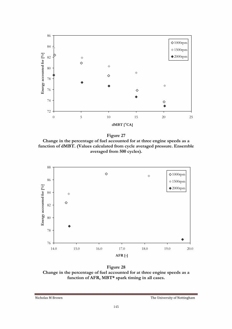
Nicholas M Brown The University of Nottingham
145
72
74
76
78
80
82
84
86
0 5 10 15 20 25
dMBT [oCA]
En
erg
y a
cco
un
ted
fo
r [%
]...
1000rpm
1500rpm
2000rpm
Figure 27
Change in the percentage of fuel accounted for at three engine speeds as a function of dMBT. (Values calculated from cycle averaged pressure. Ensemble
averaged from 500 cycles).
76
78
80
82
84
86
88
14.0 15.0 16.0 17.0 18.0 19.0 20.0
AFR [-]
En
erg
y a
cco
un
ted
fo
r [%
]...
1000rpm
1500rpm
2000rpm
Figure 28
Change in the percentage of fuel accounted for at three engine speeds as a function of AFR, MBT* spark timing in all cases.
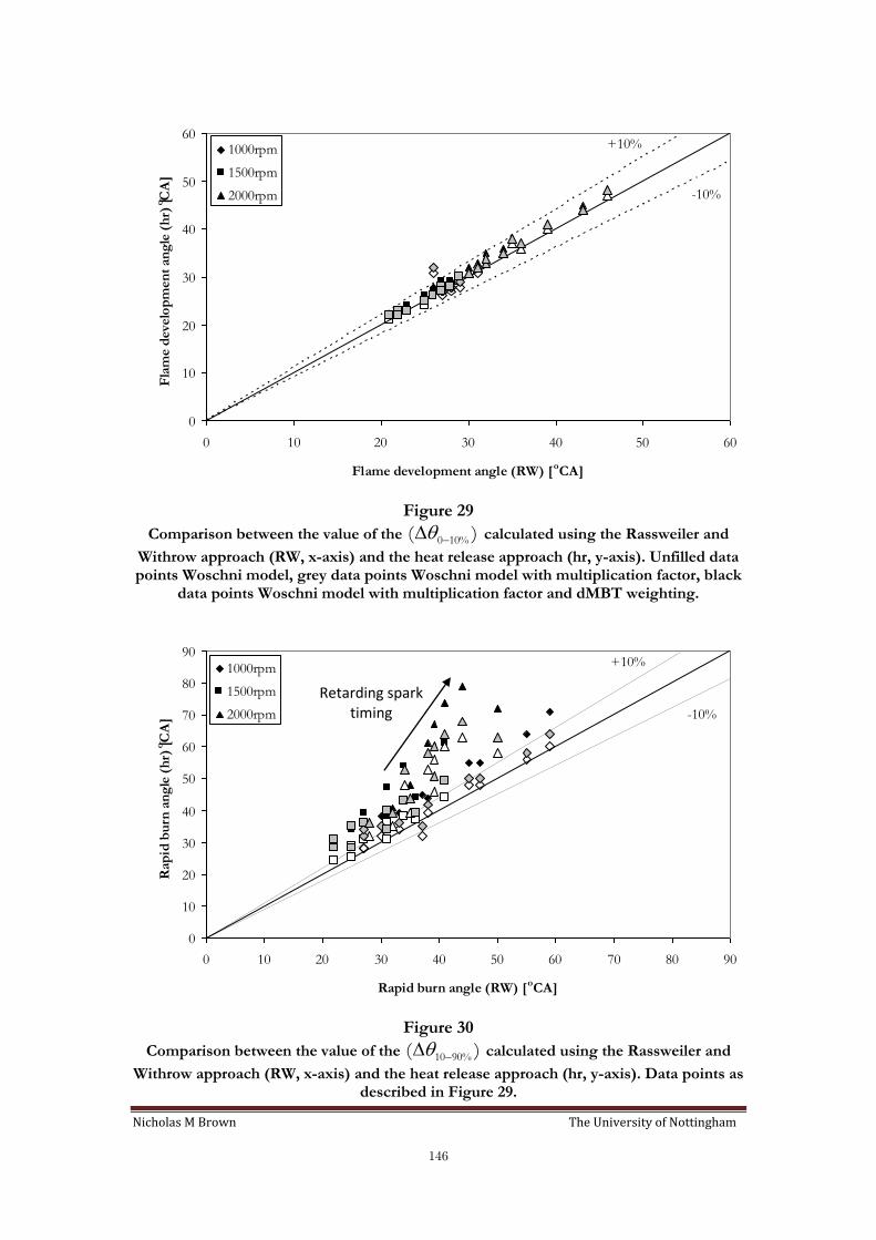
Nicholas M Brown The University of Nottingham
146
0
10
20
30
40
50
60
0 10 20 30 40 50 60
Flame development angle (RW) [oCA]
Fla
me d
eve
lop
men
t an
gle
(h
r) [o C
A].
..1000rpm
1500rpm
2000rpm
+10%
-10%
Figure 29
Comparison between the value of the 0 10%( ) calculated using the Rassweiler and
Withrow approach (RW, x-axis) and the heat release approach (hr, y-axis). Unfilled data points Woschni model, grey data points Woschni model with multiplication factor, black
data points Woschni model with multiplication factor and dMBT weighting.
0
10
20
30
40
50
60
70
80
90
0 10 20 30 40 50 60 70 80 90
Rapid burn angle (RW) [oCA]
Rap
id b
urn
an
gle
(h
r) [oC
A].
..
1000rpm
1500rpm
2000rpm
+10%
-10%
Figure 30
Comparison between the value of the 10 90%( ) calculated using the Rassweiler and
Withrow approach (RW, x-axis) and the heat release approach (hr, y-axis). Data points as described in Figure 29.
Retarding spark timing

Nicholas M Brown The University of Nottingham
147
0.0
1.0
2.0
3.0
4.0
5.0
6.0
0 200 400 600
Sample number [-]
CO
V f
lam
e d
evelo
pm
en
t an
gle
[%
]...
1000rpm
1500rpm
2000rpm
0
2
4
6
8
10
12
14
0 200 400 600
Sample number [-]
CO
V r
ap
id b
urn
an
gle
[%
]...
1000rpm
1500rpm
2000rpm
0
2
4
6
8
10
12
0 200 400 600
Sample number [-]
CO
V f
lam
e d
evelo
pm
en
t an
gle
[%
]...
1000rpm
1500rpm
2000rpm
0
5
10
15
20
25
30
35
40
0 200 400 600
Sample number [-]
CO
V r
ap
id b
urn
an
gle
[%
]...
1000rpm
1500rpm
2000rpm
Figure 31
Influence of sample size on 0 10%
COV and 10 90%
COV at (a) stable operating
conditions ( 10nIMEPCOV ) and (b) unstable operating conditions
( 10nIMEPCOV ).
a)
b)
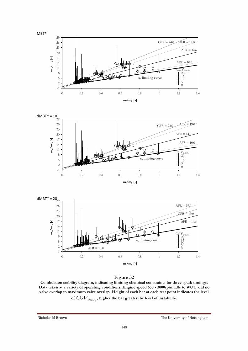
Nicholas M Brown The University of Nottingham
148
-1
2
5
8
11
14
17
20
23
26
29
0 0.2 0.4 0.6 0.8 1 1.2 1.4
mf/mb [-]
m a/
m b
[-]
...
COVIMEPn
05101520
GFR = 24.0 AFR = 19.0
AFR = 14.6
AFR = 10.0
xb limiting curve
-1
2
5
8
11
14
17
20
23
26
29
0 0.2 0.4 0.6 0.8 1 1.2 1.4
mf/mb [-]
m a/
m b
[-]
...
COVIMEPn
05101520
GFR = 23.0 AFR = 19.0
AFR = 14.6
AFR = 10.0
xb limiting curve
-1
2
5
8
11
14
17
20
23
26
29
0 0.2 0.4 0.6 0.8 1 1.2 1.4
mf/mb [-]
m a/
m b
[-]
...
COVIMEPn
05101520
GFR = 19.0
AFR = 19.0
AFR = 14.6
AFR = 10.0
xb limiting curve
Figure 32 Combustion stability diagram, indicating limiting chemical constraints for three spark timings.
Data taken at a variety of operating conditions: Engine speed 650 - 3000rpm, idle to WOT and no valve overlap to maximum valve overlap. Height of each bar at each test point indicates the level
of nIMEPCOV , higher the bar greater the level of instability.
MBT*
dMBT* = 10
dMBT* = 20
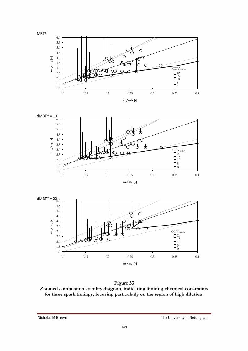
Nicholas M Brown The University of Nottingham
149
1.0
1.5
2.0
2.5
3.0
3.5
4.0
4.5
5.0
5.5
6.0
0.1 0.15 0.2 0.25 0.3 0.35 0.4
mf/mb [-]
m a/
m b
[-]
...
COVIMEPn
05101520
1.0
1.5
2.0
2.5
3.0
3.5
4.0
4.5
5.0
5.5
6.0
0.1 0.15 0.2 0.25 0.3 0.35 0.4
mf/mb [-]
m a/
m b
[-]
...
COVIMEPn
20151050
1.0
1.5
2.0
2.5
3.0
3.5
4.0
4.5
5.0
5.5
6.0
0.1 0.15 0.2 0.25 0.3 0.35 0.4
mf/mb [-]
m a/
m b
[-]
COVIMEPn
20151050
Figure 33
Zoomed combustion stability diagram, indicating limiting chemical constraints for three spark timings, focusing particularly on the region of high dilution.
MBT*
dMBT* = 10
dMBT* = 20
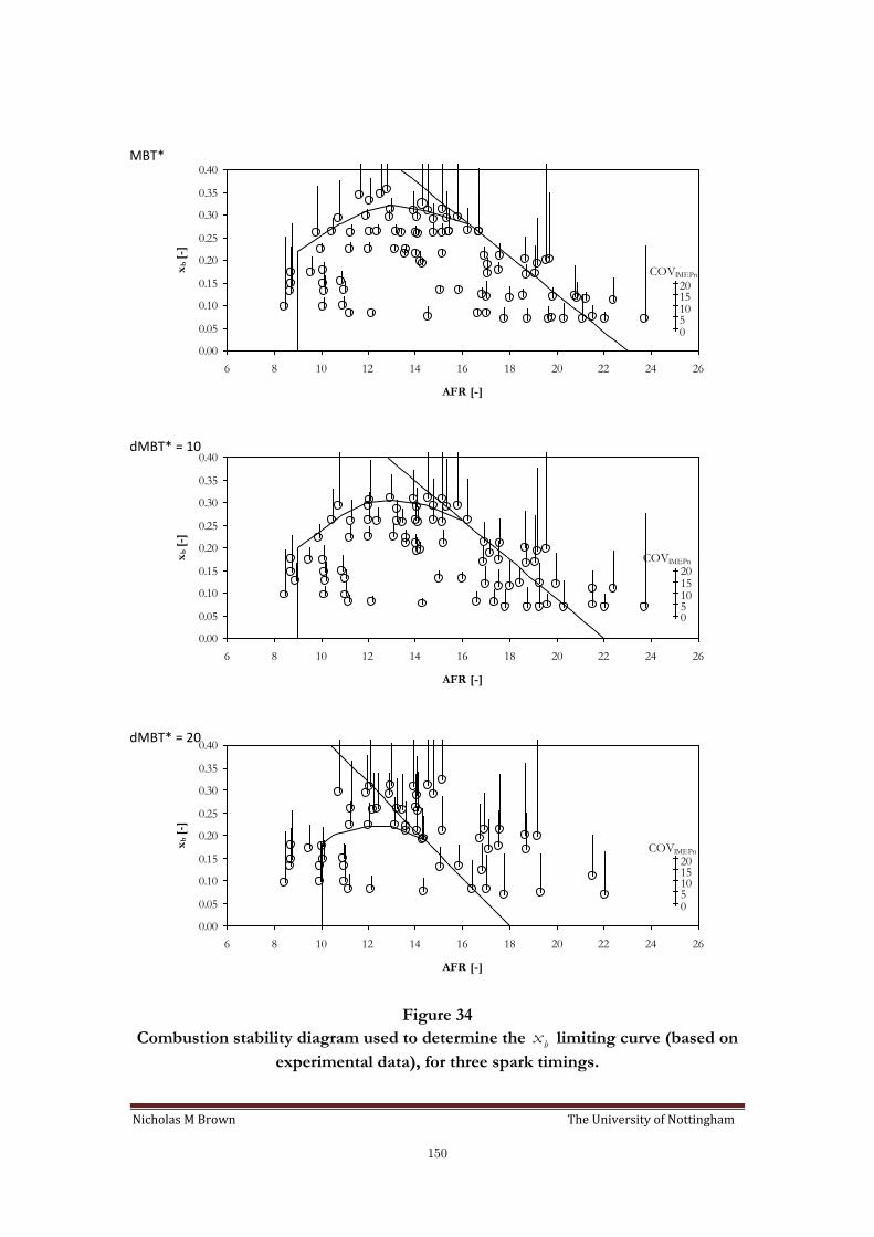
Nicholas M Brown The University of Nottingham
150
0.00
0.05
0.10
0.15
0.20
0.25
0.30
0.35
0.40
6 8 10 12 14 16 18 20 22 24 26
AFR [-]
xb
[-]
COVIMEPn
05101520
0.00
0.05
0.10
0.15
0.20
0.25
0.30
0.35
0.40
6 8 10 12 14 16 18 20 22 24 26
AFR [-]
xb
[-]
COVIMEPn
05101520
0.00
0.05
0.10
0.15
0.20
0.25
0.30
0.35
0.40
6 8 10 12 14 16 18 20 22 24 26
AFR [-]
xb
[-]
COVIMEPn
05101520
Figure 34
Combustion stability diagram used to determine the bx limiting curve (based on
experimental data), for three spark timings.
MBT*
dMBT* = 10
dMBT* = 20
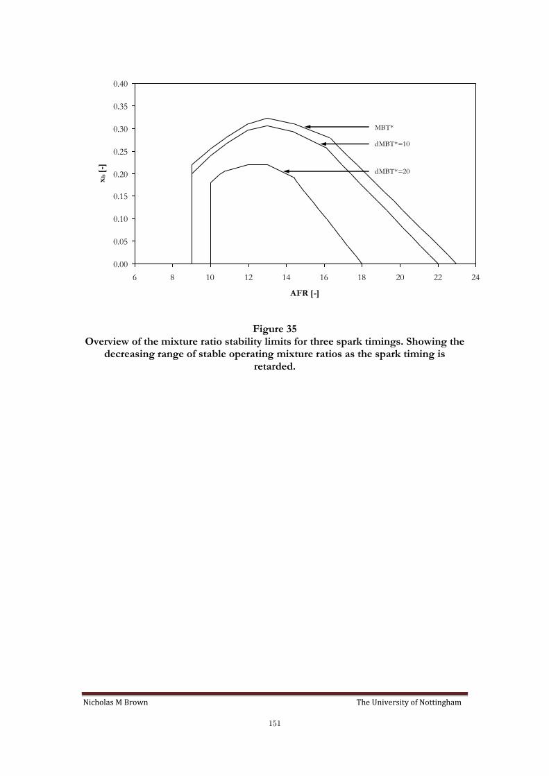
Nicholas M Brown The University of Nottingham
151
0.00
0.05
0.10
0.15
0.20
0.25
0.30
0.35
0.40
6 8 10 12 14 16 18 20 22 24
AFR [-]
xb
[-]
MBT*
dMBT*=10
dMBT*=20
Figure 35 Overview of the mixture ratio stability limits for three spark timings. Showing the
decreasing range of stable operating mixture ratios as the spark timing is retarded.

Nicholas M Brown The University of Nottingham
152
0
10
20
30
40
15 17 19 21 23 25 27 29
GFR [-]
CO
VIM
EP
n [%
]
0
10
20
30
40
15 17 19 21 23 25 27 29
GFR [-]
CO
VIM
EP
n [%
]
Figure 36
The influence of removing partial burning and misfiring cycles from the
calculation of nIMEPCOV . Where a) includes all cycles, b) has removed partial
burning and misfiring cycles. Constant fuel data black points, constant air data grey data points.
a)
b)

Nicholas M Brown The University of Nottingham
153
0
1
2
3
4
5
15 17 19 21 23 25 27 29
GFR [-]
IME
Pn [
bar
].
0
5
10
15
20
25
30
35
40
45
CO
VIM
EP
n [b
ar]
constant air test
constant fuel test
0
1
2
3
4
5
15 17 19 21 23 25 27 29
GFR [-]
IME
Pn [
bar
].
0
5
10
15
20
25
30
35
40
45
CO
VIM
EP
n [b
ar]
constant air test
constant fuel test
0
1
2
3
4
5
15 17 19 21 23 25 27 29
GFR [-]
IME
Pn [
bar
].
0
5
10
15
20
25
30
35
40
45
CO
VIM
EP
n [b
ar]
constant air test
constant fuel test
Figure 37 The change in IMEPn and COVIMEPn with GFR for two different test methods,
constant fuel tests indicated with diamonds and constant air tests indicated with squares. Where a) is 1000rpm, b) 1500rpm and c) 2000rpm.
a)
b)
c)
[%]
[%]
[%]

Nicholas M Brown The University of Nottingham
154
0
1
2
3
4
5
15 17 19 21 23 25 27 29
GFR [-]
IME
Pn [
bar]
.
0.0
0.1
0.2
0.3
0.4
0.5
0.6
0.7
0.8
std
ev
IME
Pn
[b
ar]
constant air test
constant fuel test
0
1
2
3
4
5
15 17 19 21 23 25 27 29
GFR [-]
IME
Pn [
bar
].
0.0
0.1
0.2
0.3
0.4
0.5
0.6
0.7
0.8
std
ev I
ME
Pn
[b
ar]
constant air test
constant fuel test
0
1
2
3
4
5
15 17 19 21 23 25 27 29
GFR [-]
IME
Pn [
bar]
.
0.0
0.1
0.2
0.3
0.4
0.5
0.6
0.7
0.8
std
ev
IME
Pn
[b
ar]
constant air test
constant fuel test
Figure 38 The change in IMEPn and stdev IMEPn with GFR for two different test methods, data as Figure 24. Constant fuel tests indicated with diamonds and constant air tests indicated
with squares.
a)
b)
c)

Nicholas M Brown The University of Nottingham
155
0
1
2
3
4
5
15 17 19 21 23 25 27 29
GFR [-]
IME
Pn [
bar]
.
0
5
10
15
20
25
30
Par
tial b
urn
ing
an
d
mis
firi
ng
cycle
s [%
]
constant air test
constant fuel test
0
1
2
3
4
5
15 17 19 21 23 25 27 29
GFR [-]
IME
Pn [
bar]
.
0
5
10
15
20
25
30
Part
ial b
urn
ing
an
d
mis
firi
ng
cycle
s [%
]
constant air test
constant fuel test
0
1
2
3
4
5
15 17 19 21 23 25 27 29
GFR [-]
IME
Pn [
bar]
.
0
5
10
15
20
25
30
Par
tial b
urn
ing
an
d
mis
firi
ng
cycle
s [%
]
misfire misfire partial burn partial burn
constant air test
constant fuel test
Figure 39 The change in IMEPn and % partial burning and misfiring cycles with GFR for two
different test methods, data as Figure 24. Constant fuel tests indicated with diamonds and constant air tests indicated with squares.
a)
b)
c)
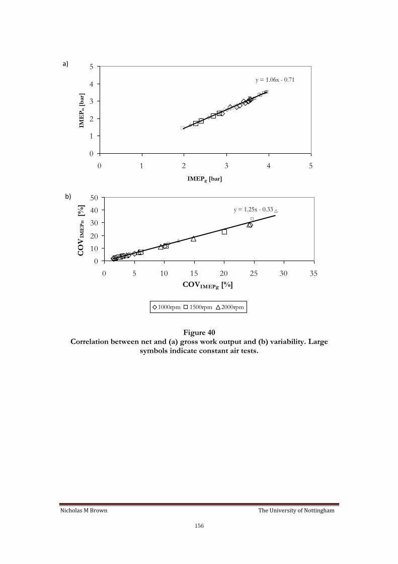
Nicholas M Brown The University of Nottingham
156
y = 1.06x - 0.71
0
1
2
3
4
5
0 1 2 3 4 5
IMEPg [bar]
IME
Pn [
bar
].
y = 1.25x - 0.33
0
10
20
30
40
50
0 5 10 15 20 25 30 35
COVIMEPg [%]
CO
VIM
EP
n [
%].
1000rpm 1500rpm 2000rpm
Figure 40 Correlation between net and (a) gross work output and (b) variability. Large
symbols indicate constant air tests.
a)
b)

Nicholas M Brown The University of Nottingham
157
0.0
1.0
2.0
3.0
4.0
5.0
6.0
7.0
8.0
0 50 100 150 200 250 300 350
oCA [-]
Pre
ssu
re [
bar]
0.90
0.95
1.00
1.05
1.10
0 50 100 150 200 250 300 350
oCA [-]
Err
or
rati
o [
-]
Figure 41 Comparison of filtered and unfiltered motored pressure cycle data, and the error
ratio between the two (unfiltered/filtered), engine speed 1500rpm

Nicholas M Brown The University of Nottingham
158
0
5
10
15
20
25
30
35
15 17 19 21 23 25 27 29
GFR [-]
CO
VIM
EP
g [%
]
dMBT* = 20
dMBT* = 15
dMBT* = 10
dMBT* = 5
dMBT* = 0
Figure 42
The influence of spark retard on gIMEPCOV over a range of GFRs. Engine speed
1000rpm, constant fuel testing.
0.00
0.10
0.20
0.30
0.40
0.50
0.60
0.70
0.80
0.90
15 17 19 21 23 25 27 29
GFR [-]
std
ev
IME
Pg
[b
ar]
dMBT* = 20
dMBT* = 15
dMBT* = 10
dMBT* = 5
dMBT* = 0
Figure 43
The influence of spark retard on stdev gIMEP over the same range of GFRs and
engine conditions as shown in Figure 42.

Nicholas M Brown The University of Nottingham
159
0.0
5.0
10.0
15.0
20.0
25.0
30.0
35.0
40.0
15 17 19 21 23 25 27 29
GFR [-]
(CO
VIM
EP
g-C
OV
*IM
EP
g)/
CO
VIM
EP
g [%
]
dMBT* = 20
dMBT* = 15
dMBT* = 10
dMBT* = 5
dMBT* = 0
Figure 44
The % difference in gIMEPCOV calculated using a constant value of mean gIMEP
based on the value at dMBT* = 0 and the normally calculated value of gIMEPCOV .

Nicholas M Brown The University of Nottingham
160
0
10
20
30
40
50
15 20 25 30
GFR [-]
CO
VIM
EP
g [%
].
0
10
20
30
40
50
15 20 25 30
GFR [-]
CO
VIM
EP
g [%
].
0
10
20
30
40
50
15 20 25 30
GFR [-]
CO
VIM
EP
g [%
].
0
10
20
30
40
50
15 20 25 30
GFR [-]
CO
VIM
EP
g [%
].
0
10
20
30
40
50
15 17 19 21 23 25 27 29
GFR [-]
CO
VIM
EP
g [%
].
1000rpm 1500rpm 2000rpm 1000rpm 1500rpm 2000rpm
retarding spark
timing
Figure 45
The change in gIMEPCOV with GFR at different spark timings, a) MBT*, b)
dMBT* = 5, c) dMBT* = 10, d) dMBT* = 15 and e) dMBT* = 20. Where the data for retarded spark timings is not corrected for the associated reduction in average
gIMEP . Open symbols constant fuel test points, filled symbols constant air test
points.
b) a)
c) d)
e)
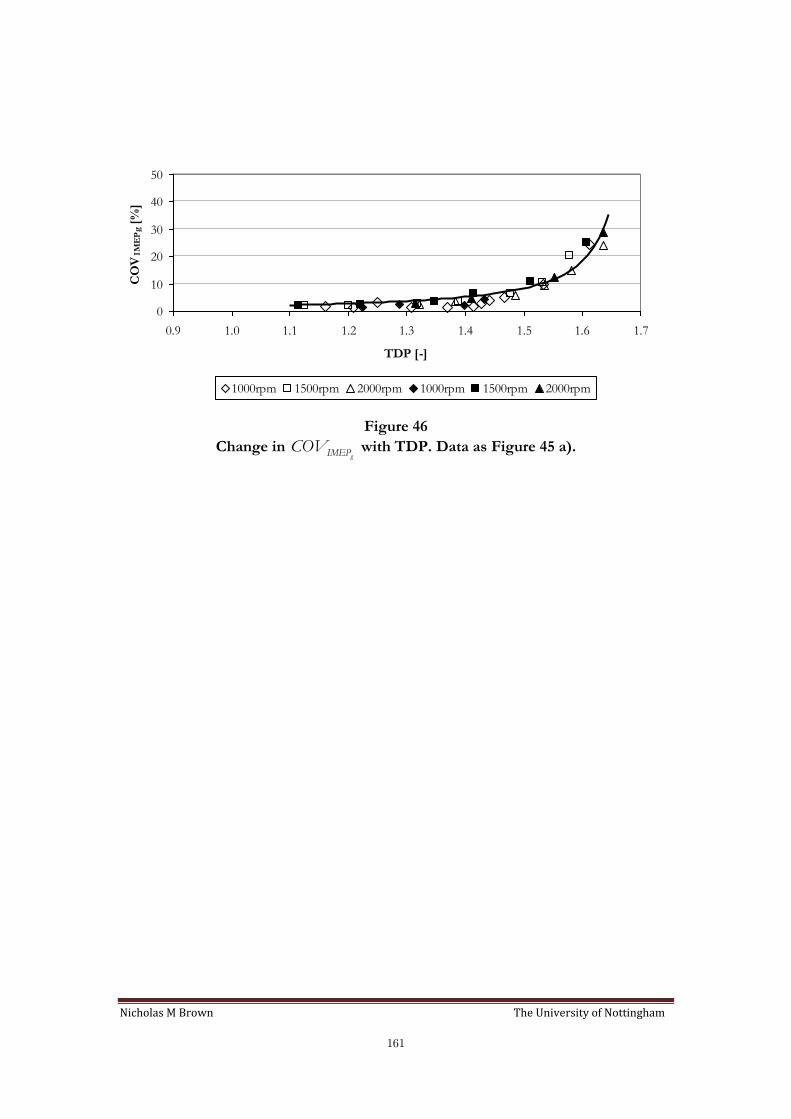
Nicholas M Brown The University of Nottingham
161
Figure 46
Change in gIMEPCOV with TDP. Data as Figure 45 a).
0
10
20
30
40
50
0.9 1.0 1.1 1.2 1.3 1.4 1.5 1.6 1.7
TDP [-]
CO
VIM
EP
g [%
].
1000rpm 1500rpm 2000rpm 1000rpm 1500rpm 2000rpm
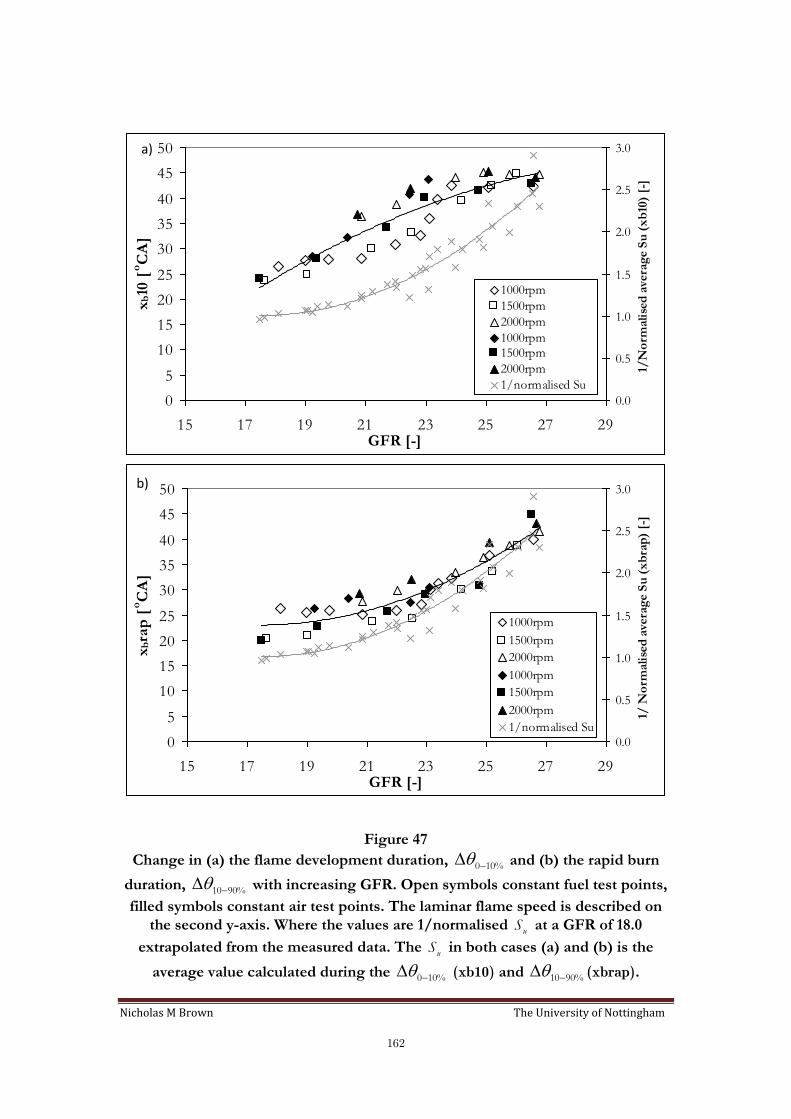
Nicholas M Brown The University of Nottingham
162
0
5
10
15
20
25
30
35
40
45
50
15 17 19 21 23 25 27 29GFR [-]
xb10
[oC
A]
0.0
0.5
1.0
1.5
2.0
2.5
3.0
1/N
orm
ali
sed
ave
rag
e S
u (
xb
10)
[-]
1000rpm
1500rpm
2000rpm
1000rpm
1500rpm
2000rpm
1/normalised Su
0
5
10
15
20
25
30
35
40
45
50
15 17 19 21 23 25 27 29GFR [-]
xbra
p [
oC
A]
0.0
0.5
1.0
1.5
2.0
2.5
3.0
1/ N
orm
ali
sed
ave
rag
e S
u (
xb
rap
) [-
]
1000rpm
1500rpm
2000rpm
1000rpm
1500rpm
2000rpm
1/normalised Su
Figure 47
Change in (a) the flame development duration, 0 10% and (b) the rapid burn
duration, 10 90% with increasing GFR. Open symbols constant fuel test points,
filled symbols constant air test points. The laminar flame speed is described on
the second y-axis. Where the values are 1/normalised uS at a GFR of 18.0
extrapolated from the measured data. The uS in both cases (a) and (b) is the
average value calculated during the 0 10% (xb10) and 10 90% (xbrap).
a)
b)

Nicholas M Brown The University of Nottingham
163
0
2
4
6
8
10
12
14
16
15 17 19 21 23 25 27 29GFR [-]
CO
Vx
b10
[%
]
1000rpm 1500rpm
2000rpm 1000rpm
1500rpm 2000rpm
0
5
10
15
20
25
30
35
40
45
15 17 19 21 23 25 27 29GFR [-]
CO
Vx
bra
p [
%]
1000rpm 1500rpm
2000rpm 1000rpm
1500rpm 2000rpm
Figure 48
Change in (a) 0 10%COV and (b) the 10 90%
COV with increasing GFR. Open
symbols constant fuel test points, filled symbols constant air test points. Values calculated as stated in Chapter 3.
a)
b)
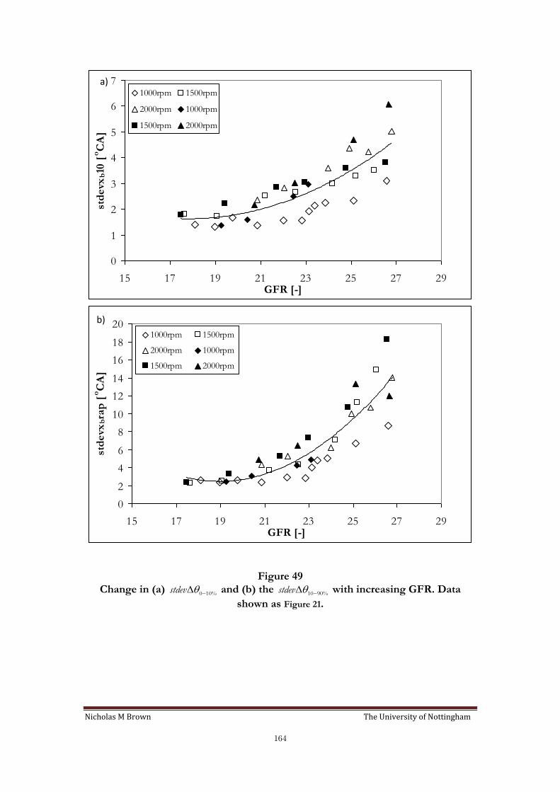
Nicholas M Brown The University of Nottingham
164
0
1
2
3
4
5
6
7
15 17 19 21 23 25 27 29GFR [-]
std
evx
b10
[oC
A]
1000rpm 1500rpm
2000rpm 1000rpm
1500rpm 2000rpm
0
2
4
6
8
10
12
14
16
18
20
15 17 19 21 23 25 27 29GFR [-]
std
evx
bra
p [
oC
A]
1000rpm 1500rpm
2000rpm 1000rpm
1500rpm 2000rpm
Figure 49
Change in (a) 0 10%stdev and (b) the 10 90%stdev with increasing GFR. Data
shown as Figure 21.
a)
b)

Nicholas M Brown The University of Nottingham
165
y = 3.10x - 2.11
R2 = 0.71
0
2
4
6
8
10
12
14
16
18
20
0.0 1.0 2.0 3.0 4.0 5.0 6.0 7.0stdevxbrap [
oCA]
std
evx
b10
[oC
A]
1000rpm 1500rpm
2000rpm 1000rpm
1500rpm 2000rpm
Figure 50
Correlation between 0 10%stdev and 10 90%stdev . Data as Figure 21.
Std
ev_
xbra
p [
oC
A]
Stdev_xb10 [oCA]
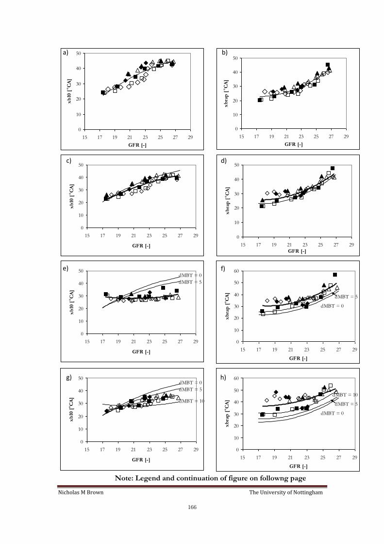
Nicholas M Brown The University of Nottingham
166
0
10
20
30
40
50
15 17 19 21 23 25 27 29
GFR [-]
xb
10 [
oC
A]
0
10
20
30
40
50
15 17 19 21 23 25 27 29
GFR [-]
xb
rap
[oC
A]
0
10
20
30
40
50
15 17 19 21 23 25 27 29
GFR [-]
xb
10 [
oC
A]
0
10
20
30
40
50
15 17 19 21 23 25 27 29
GFR [-]
xb
rap
[oC
A]
0
10
20
30
40
50
15 17 19 21 23 25 27 29
GFR [-]
xb
10 [
oC
A]
dMBT = 0
dMBT = 5
0
10
20
30
40
50
60
15 17 19 21 23 25 27 29
GFR [-]
xb
rap
[oC
A]
dMBT = 0
dMBT = 5
0
10
20
30
40
50
15 17 19 21 23 25 27 29
GFR [-]
xb
10 [
oC
A]
dMBT = 0
dMBT = 5
dMBT = 10
0
10
20
30
40
50
60
15 17 19 21 23 25 27 29
GFR [-]
xb
rap
[oC
A]
dMBT = 0
dMBT = 5
dMBT = 10
Note: Legend and continuation of figure on followng page
b) a)
c) d)
e) f)
g) h)
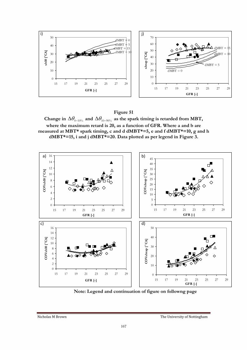
Nicholas M Brown The University of Nottingham
167
0
10
20
30
40
50
15 17 19 21 23 25 27 29
GFR [-]
xb
10 [
oC
A]
dMBT = 0
dMBT = 5
dMBT = 10 dMBT = 15
0
10
20
30
40
50
60
70
15 17 19 21 23 25 27 29
GFR [-]
xb
rap
[oC
A]
dMBT = 0
dMBT = 5
dMBT = 10
dMBT = 15
Figure 51
Change in 0 10% and 10 90% as the spark timing is retarded from MBT,
where the maximum retard is 20, as a function of GFR. Where a and b are measured at MBT* spark timing, c and d dMBT*=5, e and f dMBT*=10, g and h
dMBT*=15, i and j dMBT*=20. Data plotted as per legend in Figure 3.
0
2
4
6
8
10
12
14
16
15 17 19 21 23 25 27 29
GFR [-]
CO
Vx
b10
[oC
A]
0
5
10
15
20
25
30
35
40
45
15 17 19 21 23 25 27 29
GFR [-]
CO
Vx
bra
p [
oC
A]
0
2
4
6
8
10
12
14
16
15 17 19 21 23 25 27 29
GFR [-]
CO
Vx
b10
[oC
A]
0
10
20
30
40
50
15 17 19 21 23 25 27 29
GFR [-]
CO
Vx
bra
p [
oC
A]
Note: Legend and continuation of figure on followng page
i) j)
a) b)
c) d)
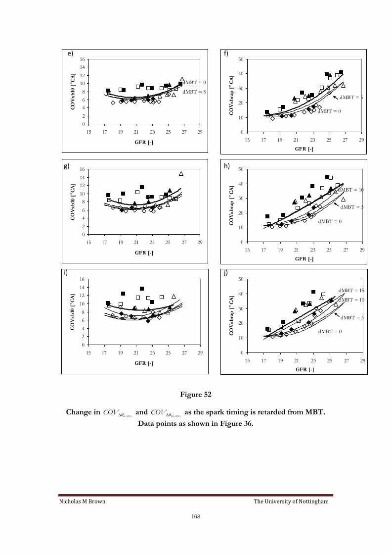
Nicholas M Brown The University of Nottingham
168
0
2
4
6
8
10
12
14
16
15 17 19 21 23 25 27 29
GFR [-]
CO
Vx
b10
[oC
A]
dMBT = 0
dMBT = 5
0
10
20
30
40
50
15 17 19 21 23 25 27 29
GFR [-]
CO
Vx
bra
p [
oC
A]
dMBT = 0
dMBT = 5
0
2
4
6
8
10
12
14
16
15 17 19 21 23 25 27 29
GFR [-]
CO
Vx
b10
[oC
A]
0
10
20
30
40
50
15 17 19 21 23 25 27 29
GFR [-]
CO
Vx
bra
p [
oC
A]
dMBT = 0
dMBT = 5
dMBT = 10
0
2
4
6
8
10
12
14
16
15 17 19 21 23 25 27 29
GFR [-]
CO
Vx
b10
[oC
A]
0
10
20
30
40
50
15 17 19 21 23 25 27 29
GFR [-]
CO
Vx
bra
p [
oC
A]
dMBT = 0
dMBT = 5
dMBT = 10
dMBT = 15
Figure 52
Change in 0 10%COV and 10 90%
COV as the spark timing is retarded from MBT.
Data points as shown in Figure 36.
e) f)
g) h)
i) j)
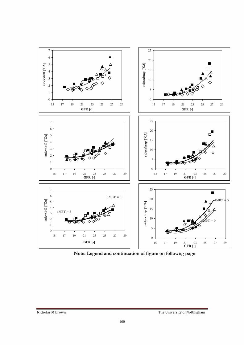
Nicholas M Brown The University of Nottingham
169
0
1
2
3
4
5
6
7
15 17 19 21 23 25 27 29
GFR [-]
std
evx
b10
[oC
A]
0
5
10
15
20
25
15 17 19 21 23 25 27 29
GFR [-]
std
evx
bra
p [
oC
A]
0
1
2
3
4
5
6
7
15 17 19 21 23 25 27 29GFR [-]
std
evx
b10
[oC
A]
0
5
10
15
20
25
15 17 19 21 23 25 27 29GFR [-]
std
evx
bra
p [
oC
A]
0
1
2
3
4
5
6
7
15 17 19 21 23 25 27 29
GFR [-]
std
evx
b10
[oC
A]
dMBT = 0
dMBT = 5
0
5
10
15
20
25
15 17 19 21 23 25 27 29GFR [-]
std
evx
bra
p [
oC
A]
dMBT = 0
dMBT = 5
Note: Legend and continuation of figure on followng page
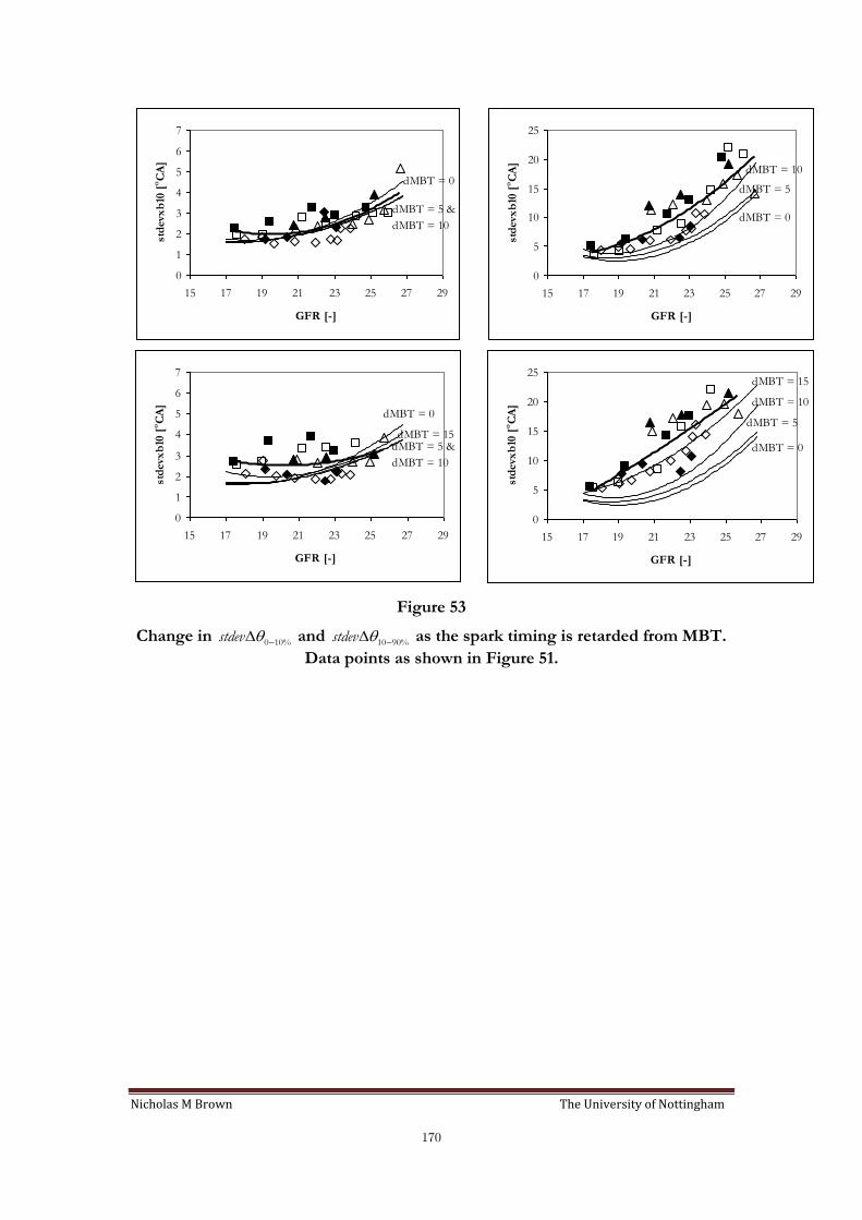
Nicholas M Brown The University of Nottingham
170
0
1
2
3
4
5
6
7
15 17 19 21 23 25 27 29
GFR [-]
std
evx
b10
[oC
A]
dMBT = 0
dMBT = 5 &
dMBT = 10
0
5
10
15
20
25
15 17 19 21 23 25 27 29
GFR [-]
std
evx
b10
[oC
A]
dMBT = 0
dMBT = 5
dMBT = 10
0
1
2
3
4
5
6
7
15 17 19 21 23 25 27 29
GFR [-]
std
evx
b10
[oC
A]
dMBT = 0
dMBT = 5 &
dMBT = 10
dMBT = 15
0
5
10
15
20
25
15 17 19 21 23 25 27 29
GFR [-]
std
evx
b10
[oC
A]
dMBT = 0
dMBT = 5
dMBT = 15
dMBT = 10
Figure 53
Change in 0 10%stdev and 10 90%stdev as the spark timing is retarded from MBT.
Data points as shown in Figure 51.

Nicholas M Brown The University of Nottingham
171
R2 = 0.7062
R2 = 0.675
R2 = 0.7512
R2 = 0.4363
R2 = 0.1926
0
5
10
15
20
25
0.0 1.0 2.0 3.0 4.0 5.0 6.0 7.0
stdevxb10 [oCA]
std
evx
bra
p [
oC
A]
MBT* dMBT*=5 dMBT*=10 dMBT*=15 dMBT*=20
MBT*
dMBT*=5
dMBT*=20
dMBT*=15dMBT*=10
Figure 54
Correlation between 0 10%stdev and 10 90%stdev for the four spark timing cases,
MBT*, dMBT*=5, dMBT*=10, dMBT*=15 and dMBT*=20. Linear trendlines used in all cases

Nicholas M Brown The University of Nottingham
172
0.0
0.2
0.4
0.6
0.8
1.0
1.2
0.6 0.7 0.8 0.9 1.0 1.1 1.2 1.3 1.4
Equivalence ratio [-]
CO
Em
issi
on
s in
dex
[-]..
..
Generic function Series 1
Generic function Series 2
Jaguar AJ27
1.6l Sigma Engine data
1.8l Zetec Engine data
2.0l I4 Engine data
richlean
Figure 55
Carbon monoxide emission index as a function of equivalence ratio for four production engines (typical design, pentroof, four valve per cylinder), at a range
of operating conditions. Specifically the AJ27 operating range is from idle (650rpm) to wide open throttle at 3500rpm, encompassing the full range of intake
cam settings.
0.00
0.02
0.04
0.06
0.08
0.10
0.12
0.14
0.16
0.18
0.20
0.6 0.7 0.8 0.9 1.0
Equivalence ratio [-]
CO
Em
issi
on
s in
dex
[-]..
..
Generic function Series 1
Generic function Series 2
Jaguar AJ27
1.6l Sigma Engine data
1.8l Zetec Engine data
2.0l I4 Engine data
Figure 56
Highlighting the improved prediction of carbon monoxide emissions index by using generic function series 2.

Nicholas M Brown The University of Nottingham
173
0.0
0.2
0.4
0.6
0.8
1.0
1.2
0.5 0.6 0.7 0.8 0.9 1.0 1.1 1.2 1.3 1.4
Equivalence ratio [-]
CO
Em
issi
on
s in
dex
[-]..
.
richlean
0
10
20
30
COVimep
Figure 57
AJ27 carbon monoxide emissions index including operating point stability information (COVIMEP). Height of each bar at each test point indicates the level of
nIMEPCOV , higher the bar greater the level of instability.
0.0
0.1
0.2
0.3
0.4
0.5
0.6
0.7
0.8
0.9
1.0
0.0 0.1 0.2 0.3 0.4 0.5 0.6 0.7 0.8 0.9 1.0
Measured CO Emissions Index [-]
Pre
dic
ted
CO
Em
issi
on
s In
dex
[-]....
stable operating conditions
unstable operating conditions
+10
-10%
Figure 58 Performance of the carbon monoxide generic function for both unstable and
stable operating points (where unstable is defined as nIMEPCOV >10).
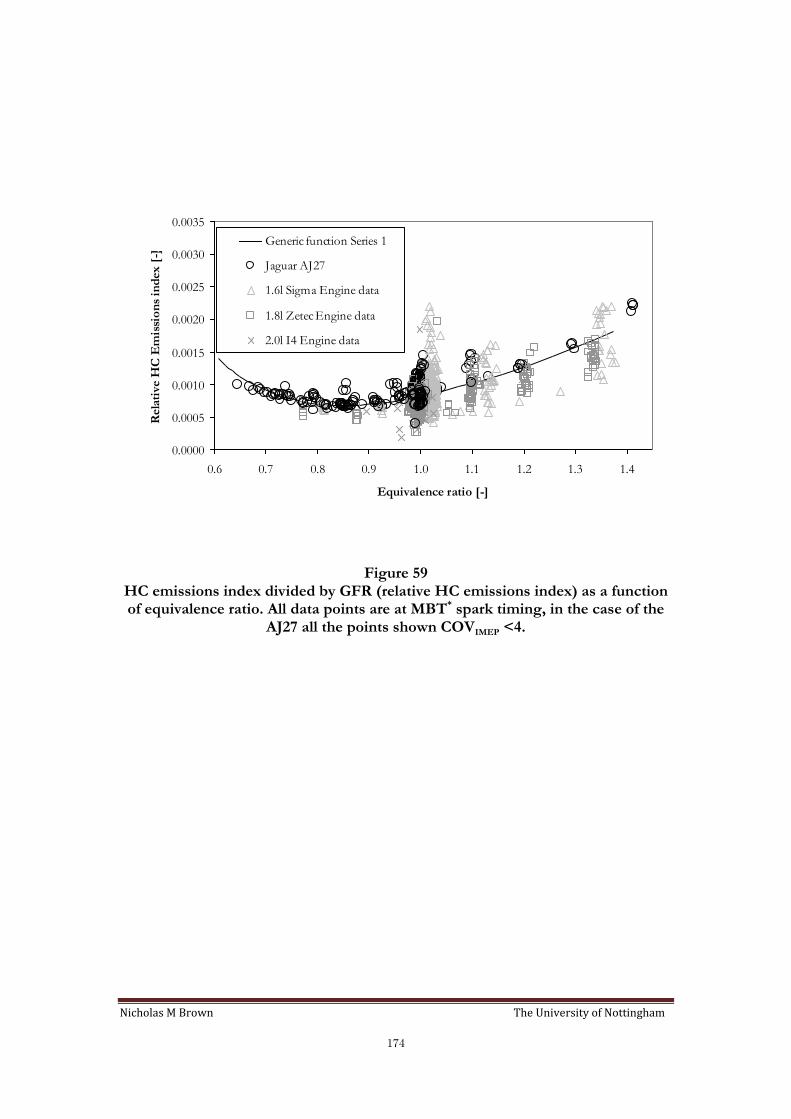
Nicholas M Brown The University of Nottingham
174
0.0000
0.0005
0.0010
0.0015
0.0020
0.0025
0.0030
0.0035
0.6 0.7 0.8 0.9 1.0 1.1 1.2 1.3 1.4
Equivalence ratio [-]
Rela
tive
HC
Em
issi
on
s in
dex
[-]....
Generic function Series 1
Jaguar AJ27
1.6l Sigma Engine data
1.8l Zetec Engine data
2.0l I4 Engine data
Figure 59 HC emissions index divided by GFR (relative HC emissions index) as a function of equivalence ratio. All data points are at MBT* spark timing, in the case of the
AJ27 all the points shown COVIMEP <4.
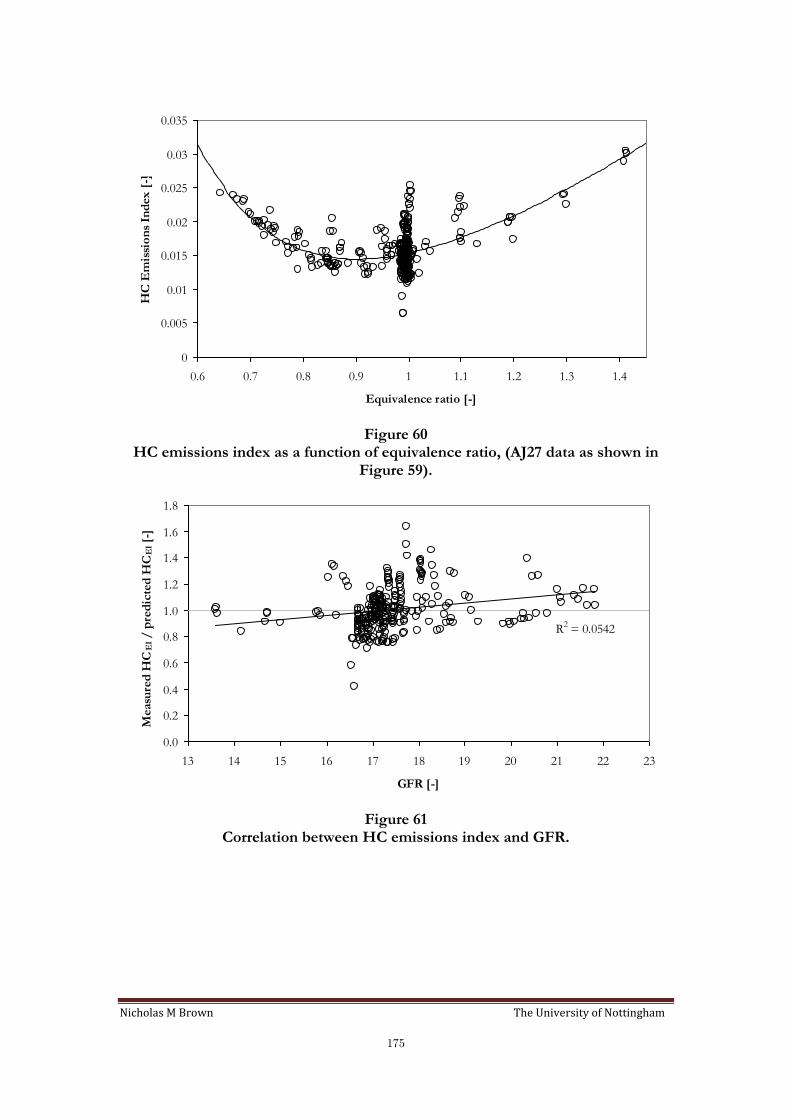
Nicholas M Brown The University of Nottingham
175
0
0.005
0.01
0.015
0.02
0.025
0.03
0.035
0.6 0.7 0.8 0.9 1 1.1 1.2 1.3 1.4
Equivalence ratio [-]
HC
Em
issi
on
s In
dex
[-]..
.
Figure 60
HC emissions index as a function of equivalence ratio, (AJ27 data as shown in Figure 59).
R2 = 0.0542
0.0
0.2
0.4
0.6
0.8
1.0
1.2
1.4
1.6
1.8
13 14 15 16 17 18 19 20 21 22 23
GFR [-]
Measu
red
HC
EI /
pre
dic
ted
HC
EI [-
]....
Figure 61
Correlation between HC emissions index and GFR.
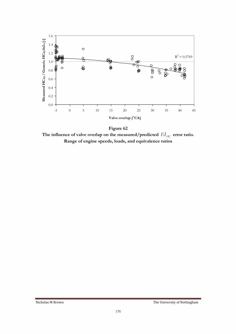
Nicholas M Brown The University of Nottingham
176
R2 = 0.5769
0.0
0.2
0.4
0.6
0.8
1.0
1.2
1.4
1.6
-5 0 5 10 15 20 25 30 35 40 45
Valve overlap [oCA]
Measu
red
HC
EI /
Gen
eri
c H
C E
I fn
2 b [
-]
Figure 62
The influence of valve overlap on the measured/predicted HCEI error ratio.
Range of engine speeds, loads, and equivalence ratios

Nicholas M Brown The University of Nottingham
177
0.0
0.2
0.4
0.6
0.8
1.0
1.2
-25 -20 -15 -10 -5 0 5 10 15 20 25 30 35
MBTD [oCA]
No
rmali
sed
HC
Em
issi
on
s In
dex
[-]....
AFR 11.0
AFR 13.0
AFR 14.6
AFR 17.0 AFR 17.0
AFR 14.6
AFR 11.0
AFR 13.0
Figure 63
The effect of spark timing changes relative to the optimum for four different AFRs. The lines through the data are formed using the generic function 4b.
0.00
0.01
0.02
0.03
0.04
0.05
0.06
0.00 0.01 0.02 0.03 0.04 0.05 0.06
Measured HC Emissions Index [-]
Pre
dic
ted
HC
Em
issi
on
s In
dex
[-]...
-30% error
+30% error
Figure 64
Overall performance of the HC generic function (equivalence ratio, valve overlap and dMBT). Idle to 3500rpm WOT, valve overlap from -5 to 42oCA and dMBT -15
to 20oCA.
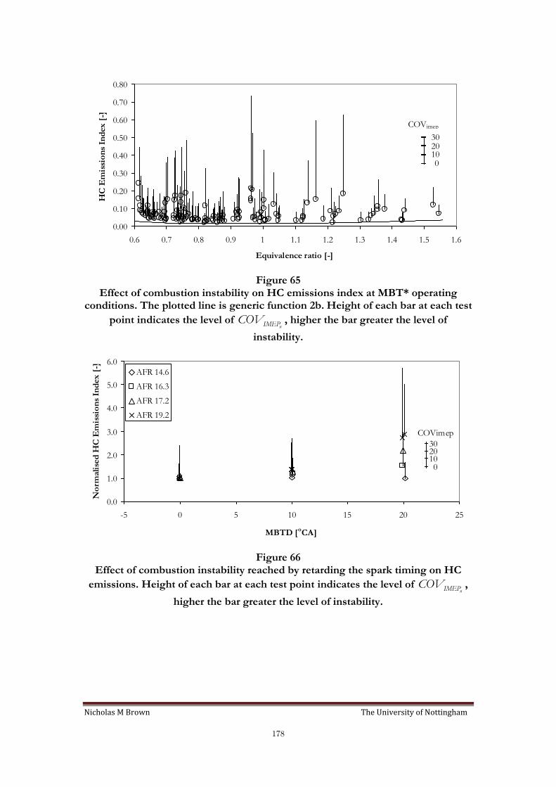
Nicholas M Brown The University of Nottingham
178
0.00
0.10
0.20
0.30
0.40
0.50
0.60
0.70
0.80
0.6 0.7 0.8 0.9 1 1.1 1.2 1.3 1.4 1.5 1.6
Equivalence ratio [-]
HC
Em
issi
on
s In
dex
[-]..
..
COVimep
3020100
Figure 65
Effect of combustion instability on HC emissions index at MBT* operating conditions. The plotted line is generic function 2b. Height of each bar at each test
point indicates the level of nIMEPCOV , higher the bar greater the level of
instability.
0.0
1.0
2.0
3.0
4.0
5.0
6.0
-5 0 5 10 15 20 25
MBTD [oCA]
No
rmali
sed
HC
Em
issi
on
s In
dex
[-]....
AFR 14.6
AFR 16.3
AFR 17.2
AFR 19.2
COVimep
3020100
Figure 66
Effect of combustion instability reached by retarding the spark timing on HC
emissions. Height of each bar at each test point indicates the level of nIMEPCOV ,
higher the bar greater the level of instability.
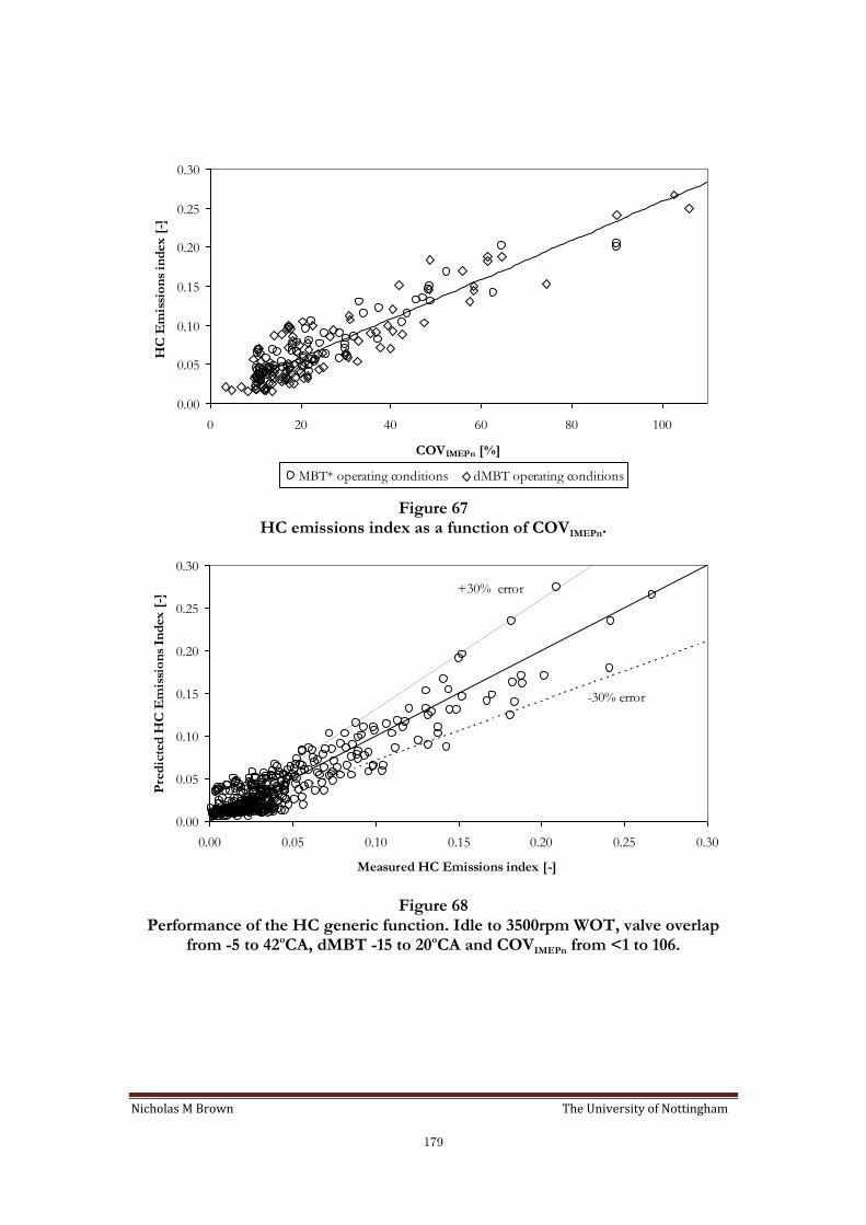
Nicholas M Brown The University of Nottingham
179
0.00
0.05
0.10
0.15
0.20
0.25
0.30
0 20 40 60 80 100
COVIMEPn [%]
HC
Em
issi
on
s in
dex
[-]..
..
MBT* operating conditions dMBT operating conditions
Figure 67
HC emissions index as a function of COVIMEPn.
0.00
0.05
0.10
0.15
0.20
0.25
0.30
0.00 0.05 0.10 0.15 0.20 0.25 0.30
Measured HC Emissions index [-]
Pre
dic
ted
HC
Em
issi
on
s In
dex
[-]....
-30% error
+30% error
Figure 68
Performance of the HC generic function. Idle to 3500rpm WOT, valve overlap from -5 to 42oCA, dMBT -15 to 20oCA and COVIMEPn from <1 to 106.

Nicholas M Brown The University of Nottingham
180
0.00
0.02
0.04
0.06
0.08
0.10
0.12
0.14
10 12 14 16 18 20 22 24 26
GFR [-]
NO
x E
mis
sio
ns
Ind
ex
[-]..
..
10.6
13.3
14.6
15.317.1
Figure 69
NOx emissions index as a function of GFR over a range of AFRs for the AJ27, operating at MBT* spark timing. The range of GFR at a given AFR result from
variations in load and valve overlap.
0.0
0.2
0.4
0.6
0.8
1.0
1.2
1.4
-5 0 5 10 15 20 25 30 35 40 45
Valve overlap [oCA]
Measu
red
NO
x EI /
Gen
eri
c N
Ox E
I fn
7 [
-]
Figure 70
The influence of valve overlap on the measured/predicted xNOEI error ratio.
Range of engine speeds, loads, and AFRs at MBT* spark timing.
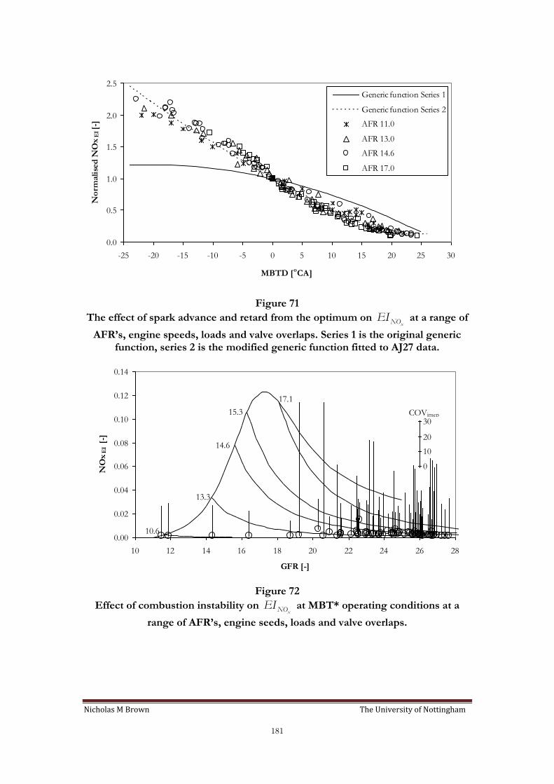
Nicholas M Brown The University of Nottingham
181
0.0
0.5
1.0
1.5
2.0
2.5
-25 -20 -15 -10 -5 0 5 10 15 20 25 30
MBTD [oCA]
No
rmali
sed
NO
x E
I [-]
Generic function Series 1
Generic function Series 2
AFR 11.0
AFR 13.0
AFR 14.6
AFR 17.0
Figure 71
The effect of spark advance and retard from the optimum on xNOEI at a range of
AFR’s, engine speeds, loads and valve overlaps. Series 1 is the original generic function, series 2 is the modified generic function fitted to AJ27 data.
0.00
0.02
0.04
0.06
0.08
0.10
0.12
0.14
10 12 14 16 18 20 22 24 26 28
GFR [-]
NO
x E
I [
-]
10.6
13.3
14.6
15.3
17.1
0
10
20
30COVimep
Figure 72
Effect of combustion instability on xNOEI at MBT* operating conditions at a
range of AFR’s, engine seeds, loads and valve overlaps.
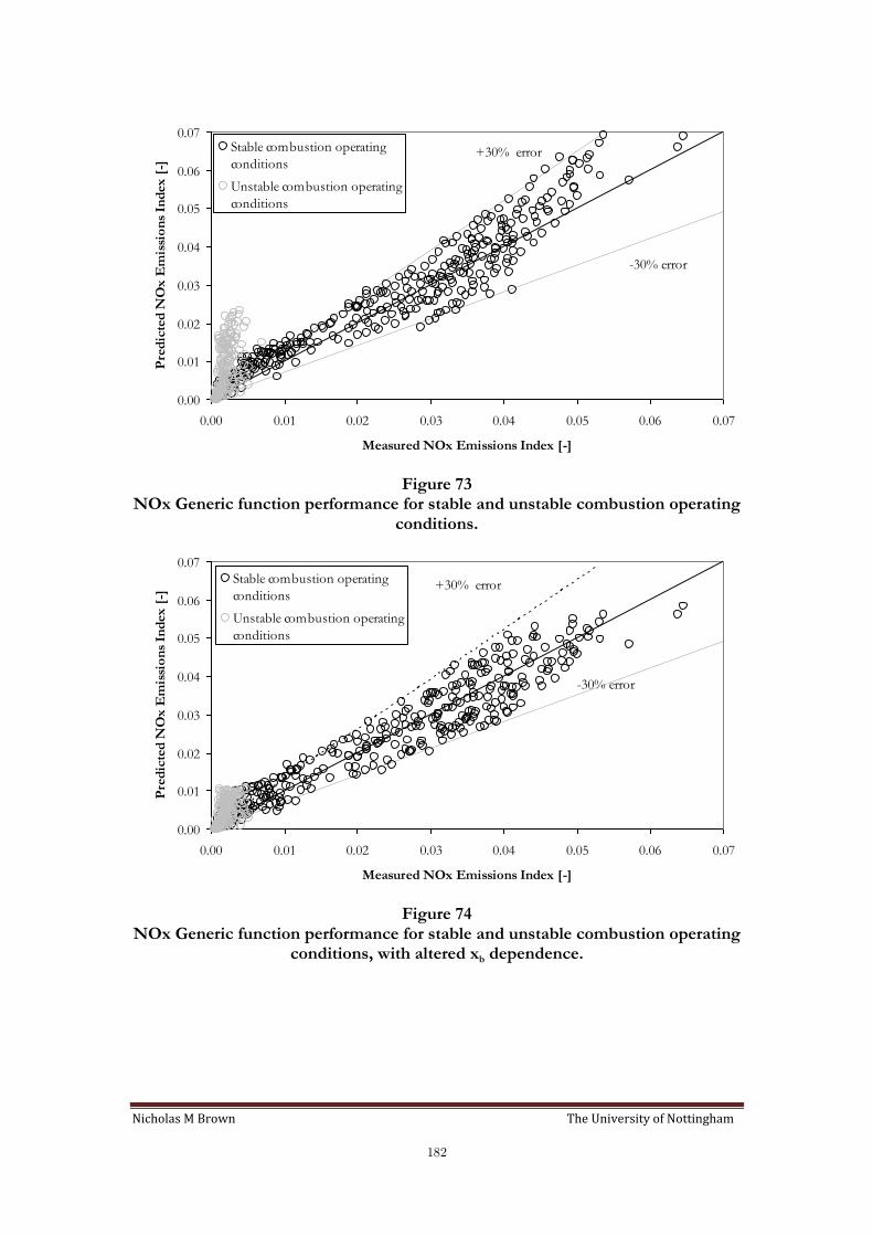
Nicholas M Brown The University of Nottingham
182
0.00
0.01
0.02
0.03
0.04
0.05
0.06
0.07
0.00 0.01 0.02 0.03 0.04 0.05 0.06 0.07
Measured NOx Emissions Index [-]
Pre
dic
ted
NO
x E
mis
sio
ns
Ind
ex
[-]
... Stable combustion operating
conditions
Unstable combustion operating
conditions
+30% error
-30% error
Figure 73
NOx Generic function performance for stable and unstable combustion operating conditions.
0.00
0.01
0.02
0.03
0.04
0.05
0.06
0.07
0.00 0.01 0.02 0.03 0.04 0.05 0.06 0.07
Measured NOx Emissions Index [-]
Pre
dic
ted
NO
x E
mis
sio
ns
Ind
ex
[-]...
Stable combustion operating
conditions
Unstable combustion operating
conditions
+30% error
-30% error
Figure 74
NOx Generic function performance for stable and unstable combustion operating conditions, with altered xb dependence.

Nicholas M Brown The University of Nottingham
183
0.0
0.5
1.0
1.5
2.0
2.5
3.0
3.5
4.0
-5 0 5 10 15 20 25 30
MBTD [oCA]
No
rmali
sed
NO
x E
I [-
]AFR 14.6
AFR 16.3
AFR 17.2
AFR 19.2
Generic function Series 2COVimep
30
20
10
0
Figure 75
Effect of combustion instability reached by retarding the spark timing on xNOEI .
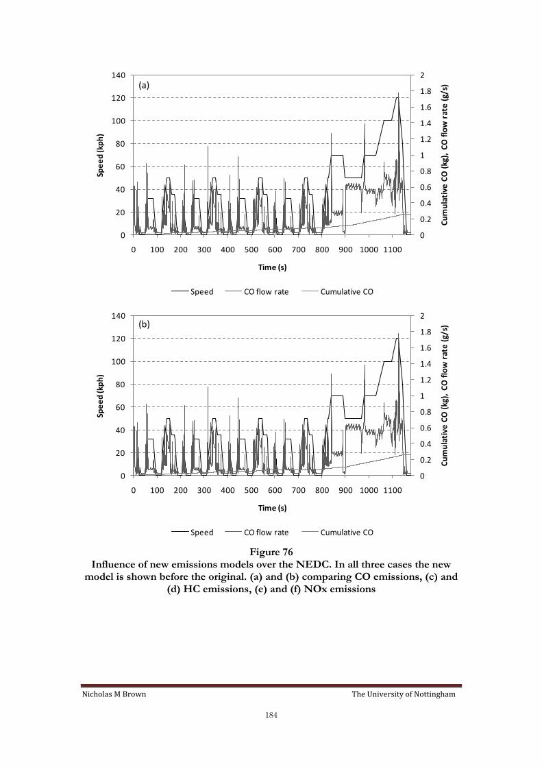
Nicholas M Brown The University of Nottingham
184
0
0.2
0.4
0.6
0.8
1
1.2
1.4
1.6
1.8
2
0
20
40
60
80
100
120
140
0 100 200 300 400 500 600 700 800 900 1000 1100
Cu
mu
lati
ve C
O (
kg),
CO
flo
w r
ate
(g/
s)
Spe
ed
(kp
h)
Time (s)
Speed CO flow rate Cumulative CO
0
0.2
0.4
0.6
0.8
1
1.2
1.4
1.6
1.8
2
0
20
40
60
80
100
120
140
0 100 200 300 400 500 600 700 800 900 1000 1100
Cu
mu
lati
ve C
O (
kg),
CO
flo
w r
ate
(g/
s)
Spe
ed
(kp
h)
Time (s)
Speed CO flow rate Cumulative CO
Figure 76 Influence of new emissions models over the NEDC. In all three cases the new
model is shown before the original. (a) and (b) comparing CO emissions, (c) and (d) HC emissions, (e) and (f) NOx emissions
(a)
(b)

Nicholas M Brown The University of Nottingham
185
0
0.05
0.1
0.15
0.2
0.25
0
20
40
60
80
100
120
140
0 100 200 300 400 500 600 700 800 900 1000 1100
Cu
mu
lati
ve H
C (
kg),
HC
flo
w r
ate
(g/
s)
Spe
ed
(kp
h)
Time (s)
Speed HC flow rate Cumulative HC
0
0.05
0.1
0.15
0.2
0.25
0
20
40
60
80
100
120
140
0 100 200 300 400 500 600 700 800 900 1000 1100
Cu
mu
lati
ve H
C (
kg),
HC
flo
w r
ate
(g/
s)
Spe
ed
(kp
h)
Time (s)
Speed HC flow rate Cumulative HC
Figure 76 Influence of new emissions models over the NEDC. In all three cases the new
model is shown before the original. (a) and (b) comparing CO emissions, (c) and (d) HC emissions, (e) and (f) NOx emissions
(c)
(d)

Nicholas M Brown The University of Nottingham
186
0
0.02
0.04
0.06
0.08
0.1
0.12
0
20
40
60
80
100
120
140
0 100 200 300 400 500 600 700 800 900 1000 1100
Cu
mu
lati
ve N
Ox
(kg)
, N
Ox
flo
w r
ate
(g/
s)
Spe
ed
(kp
h)
Time (s)
Speed NOx flow rate Cumulative NOx
0
0.02
0.04
0.06
0.08
0.1
0.12
0.14
0
20
40
60
80
100
120
140
0 100 200 300 400 500 600 700 800 900 1000 1100
Cu
mu
lati
ve N
Ox
(kg)
, N
Ox
flo
w r
ate
(g/
s)
Spe
ed
(kp
h)
Time (s)
Speed NOx flow rate Cumulative NOx
Figure 76
Influence of new emissions models over the NEDC. In all three cases the new model is shown before the original. (a) and (b) comparing CO emissions, (c) and
(d) HC emissions, (e) and (f) NOx emissions
(e)
(f)

Nicholas M Brown The University of Nottingham
187
-0.03
-0.02
-0.01
0
0.01
0.02
0.03
0.04
0.05
0.06
0.07
0 100 200 300 400 500 600 700 800 900 1000 1100
dif
CO
, HC
an
d N
Ox
flo
w r
ate
(g/
s)
Time (s)
dif CO dif HC dif NOx
Figure 77 Difference plots (New emissions flow rate – Old emissions flow rate) over the
NEDC. (note difference between old and new CO mostly 0, hence it appears no data plotted)
0
20
40
60
80
100
120
140
160
180
200
-5 0 5 10 15 20 25
Spark timing [°CA]
To
rqu
e [
Nm
]
MBT* MBT
over extrapolated MBT* and MBT
Figure 78
Knock limited spark sweep at high loads causing over extrapolation of MBT* and MBT spark timing.

Nicholas M Brown The University of Nottingham
188
R2 = 0.97
0.0
0.5
1.0
1.5
2.0
2.5
-25 -20 -15 -10 -5 0 5 10 15 20 25
MBTD [oCA]
No
rmali
sed
NO
x E
I [-
]
Figure 79
Linear relationship between relative spark timing (-23 to 16) and normalised
xNOEI . Eight individual spark sweeps at 650rpm, 1500rpm, 2000rpm and
3000rpm, light and medium load. Baseline is 0.12 of MBT* xNOEI .
-5
0
5
10
15
20
25
0.000 0.005 0.010 0.015 0.020 0.025 0.030 0.035 0.040
NOx Emissions Index [-]
Sp
ark
tim
ing
[oC
A]
Figure 80
The application of the method to calculate relative spark timing from measured
xNOEI .
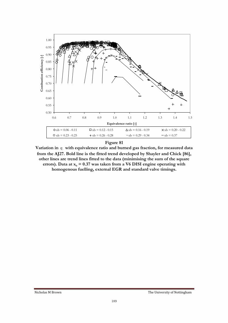
Nicholas M Brown The University of Nottingham
189
0.50
0.55
0.60
0.65
0.70
0.75
0.80
0.85
0.90
0.95
1.00
0.6 0.7 0.8 0.9 1.0 1.1 1.2 1.3 1.4 1.5
Equivalence ratio [-]
Co
mb
ust
ion
eff
icie
ncy [
-]...
xb = 0.06 - 0.11 xb = 0.12 - 0.15 xb = 0.16 - 0.19 xb = 0.20 - 0.22
xb = 0.23 - 0.25 xb = 0.26 - 0.28 xb = 0.29 - 0.34 xb = 0.37
Figure 81 Variation in c with equivalence ratio and burned gas fraction, for measured data
from the AJ27. Bold line is the fitted trend developed by Shayler and Chick [86], other lines are trend lines fitted to the data (minimising the sum of the square
errors). Data at xb = 0.37 was taken from a V6 DISI engine operating with homogenous fuelling, external EGR and standard valve timings.

Nicholas M Brown The University of Nottingham
190
0.0
0.2
0.4
0.6
0.8
1.0
1.2
0.6 0.7 0.8 0.9 1.0 1.1 1.2 1.3 1.4
Equivalence ratio [-]
CO
Em
issi
on
s in
dex
[-]..
.CO generic function
Equilibrium at the end of expansion
Equilibrium at measured exhaust port temperature
Equilibrium at peak burned gas temperatures and
pressures
min
max
mean
Figure 82
COEI , generic function and calculated at points throughout the cycle.
0.0
0.2
0.4
0.6
0.8
1.0
1.2
1.4
0.7 0.8 0.9 1.0 1.1 1.2 1.3 1.4
Equivalence Ratio [-]
CO
Em
issi
on
s In
dex
[-]..
.
Newhall kinetic model
COEI generic function
Figure 83
Comparison between the Newhall [89] kinetic model used to predict COEI and
the COEI generic function.

Nicholas M Brown The University of Nottingham
191
0.0
0.2
0.4
0.6
0.8
1.0
1.2
1.4
0.7 0.8 0.9 1.0 1.1 1.2 1.3 1.4
Equivalence Ratio [-]
CO
Em
issi
on
s In
dex
[-]..
.
COEI equilbrium at
1800K (3) COEI partial equilibrium
model [5] (2) Partially oxidised
HC emissions (1)
Figure 84
The COEI generic function, highlighting the production mechanisms of CO.
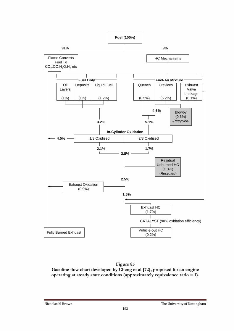
Nicholas M Brown The University of Nottingham
192
Figure 85 Gasoline flow chart developed by Cheng et al [72], proposed for an engine operating at steady state conditions (approximately equivalence ratio = 1).
Fuel (100%)
Flame Converts
Fuel To
CO2,CO,H
2O,H
2 etc
91%
HC Mechanisms
9%
Fuel-Air MixtureFuel Only
Exhuast
Valve
Leakage
(0.1%)
Oil
Layers
(1%)
Deposits
(1%)
Liquid Fuel
(1.2%)
Quench
(0.5%)
Crevices
(5.2%)
In-Cylinder Oxidation
3.2%
4.6%Blowby
(0.6%)
-Recycled-5.1%
1/3 Oxidised 2/3 Oxidised
2.1% 1.7%
3.8%
Residual
Unburned HC
(1.3%)
-Recycled-
2.5%
Exhaust Oxidation
(0.9%)
1.6%
Fully Burned Exhuast
Exhuast HC
(1.7%)
CATALYST (90% oxidation efficiency)
Vehicle-out HC
(0.2%)
4.5%

Nicholas M Brown The University of Nottingham
193
0
0.005
0.01
0.015
0.02
0.025
0.03
0.035
0.6 0.7 0.8 0.9 1 1.1 1.2 1.3 1.4
Equivalence ratio [-]
HC
Em
issi
on
s In
dex
[-]..
.
Figure 86 HC emissions index as a function of equivalence ratio
0.000
0.005
0.010
0.015
0.020
0.025
0.030
0.035
0.6 0.7 0.8 0.9 1.0 1.1 1.2 1.3 1.4
Equivalence ratio [-]
HC
Em
issi
on
s In
dex
[-]..
.
EIHC generic function
BULK GAS EIHC
NORMAL EIHC
Figure 87
HC emissions index as a function of equivalence ratio
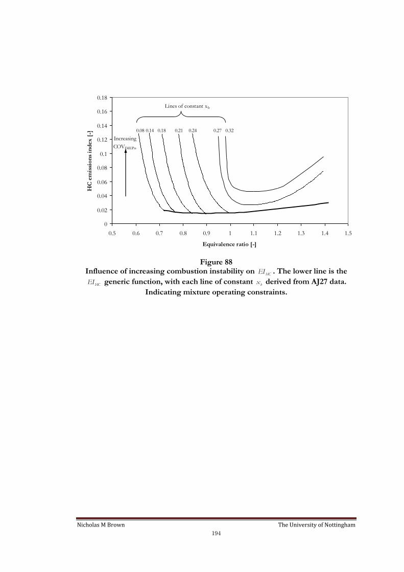
Nicholas M Brown The University of Nottingham
194
0
0.02
0.04
0.06
0.08
0.1
0.12
0.14
0.16
0.18
0.5 0.6 0.7 0.8 0.9 1 1.1 1.2 1.3 1.4 1.5
Equivalence ratio [-]
HC
em
issi
on
s in
dex
[-]..
.
Lines of constant xb
0.08 0.14 0.18 0.21 0.24 0.27 0.32
Increasing
COVIMEPn
Figure 88
Influence of increasing combustion instability on HCEI . The lower line is the
HCEI generic function, with each line of constant bx derived from AJ27 data.
Indicating mixture operating constraints.

Nicholas M Brown The University of Nottingham
195
0
2000
4000
6000
8000
10000
12000
0 2 4 6 8 10 12 14 16 18 20
Time [ms]
NO
[p
pm
]Pressure = 1000kPa
= 0.9T = 2700K
T = 2600K
T = 2500K
T = 2400K
T = 2200K
Equilib rium (2700K)
Equilib rium (2600K)
Equilib rium (2500K)
Equilib rium (2400K)
Equilib rium (2200K)
0
1000
2000
3000
4000
5000
6000
7000
8000
0 2 4 6 8 10 12 14 16 18 20
Time [ms]
NO
[p
pm
]
Pressure = 1000kPa
= 1.0
0
500
1000
1500
2000
2500
3000
3500
4000
4500
5000
0 2 4 6 8 10 12 14 16 18 20
Time [ms]
NO
[p
pm
]
Pressure = 1000kPa
= 1.1
Figure 89
NO concentration as a function of time for five temperatures at 1000kPa and three equivalence ratios.

Nicholas M Brown The University of Nottingham
196
2250
2300
2350
2400
2450
2500
2550
2600
10.0 12.0 14.0 16.0 18.0 20.0 22.0 24.0 26.0
GFR [-]
Ad
iab
ati
c f
lam
e t
em
pera
ture
[K
]...
0.00
0.05
0.10
0.15
0.20
0.25
NO
em
issi
on
s in
dex
[-]..
.
EINOx generic function
Equilibrium NO at
adiabatic flame temperature
NOEI at 2 - 16ms
in 2ms incremetns
Figure 90
NOEI as a function of GFR (where GFR = AFR+1, xb=0), adiabatic flame
temperature as a function of GFR and the xNOEI generic function (as modified
for the AJ27). (All modelled calculations were based on iso-octane and have been offset to account for the difference in stoichiometric AFR compared to gasoline).
1800
1900
2000
2100
2200
2300
2400
2500
2600
2700
10 12 14 16 18 20 22 24 26
GFR [-]
Ad
iab
ati
c f
lam
e t
em
pera
ture
[K
]....
10.3
11.1
12.1
13.2 14.6
16.3
17.3
18.4
19.6
Figure 91 Adiabatic flame temperature as a function of GFR for lines of constant AFR. The upper curve is the locus point where bx is zero, moving down the constant AFR
curve bx increases from 0:0.05:0.25.
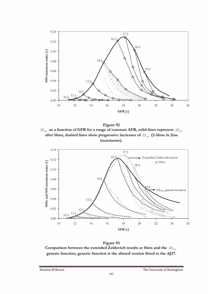
Nicholas M Brown The University of Nottingham
197
0.00
0.02
0.04
0.06
0.08
0.10
0.12
0.14
10 12 14 16 18 20 22 24 26
GFR [-]
NO
em
issi
on
s in
dex
[-]..
.
10.311.1
12.1
13.2
14.6
16.3
17.3
18.4
19.6
Figure 92
NOEI as a function of GFR for a range of constant AFR, solid lines represent NOEI
after 16ms, dashed lines show progressive increases of NOEI (2-16ms in 2ms
increments).
0.00
0.02
0.04
0.06
0.08
0.10
0.12
0.14
10 12 14 16 18 20 22 24 26
GFR [-]
NO
x a
nd
NO
em
issi
on
s in
dex
[-]...
10.311.1
12.1
13.2
14.6
16.3
17.3
18.4
19.6
Extended Zeldovich curves
at 16ms
EINOx generic function
Figure 93 Comparison between the extended Zeldovich results at 16ms and the
xNOEI
generic function, generic function is the altered version fitted to the AJ27.

Nicholas M Brown The University of Nottingham
198
0.0
0.2
0.4
0.6
0.8
1.0
-40 -30 -20 -10 0 10 20 30 40
Crank Angle [oATDC]
xb
[-]
increasing n, (2:1:9),
a = 2
n 0-10% 10-90%
2 10 43
3 15 42
4 20 42
5 23 42
6 25 41
7 27 41
8 28 41
9 28 41
0.0
0.2
0.4
0.6
0.8
1.0
-60 -50 -40 -30 -20 -10 0 10 20 30 40
Crank Angle [oATDC]
xb
[-] increasing a, (2:1:9),
n = 2
a 0-10% 10-90%
2 10 43
3 8 36
4 7 31
5 6 28
6 6 25
7 5 23
8 5 22
9 5 21
Figure 94 The effect of increasing a (efficiency factor) and n (form factor) on the shape of
the burned mass fraction curve produced from the Wiebe function and the related changes in the 10bx and bx rap .

Nicholas M Brown The University of Nottingham
199
y = 1.2x - 0.9
R² = 0.998
3.0
4.0
5.0
6.0
7.0
8.0
9.0
3.0 4.0 5.0 6.0 7.0 8.0 9.0
a c
alc
ula
ted
fro
m d
ura
tio
n d
efi
ned
as
90%
[-]
a calculated from duration defined as 99% [-]
Figure 95
Correlation between a calculated from the dq defined as 99% and 90%.
y = 1.0x - 0.1
R² = 0.994
2.0
2.5
3.0
3.5
4.0
4.5
5.0
5.5
6.0
6.5
7.0
2.0 3.0 4.0 5.0 6.0 7.0
n
n calculated from duration defined as 99% [-]
Figure 96
Correlation between n calculated from the dq defined as 99% and 90%.

Nicholas M Brown The University of Nottingham
200
y = 0.168x + 2.523 @ MBT*
y = 0.175x + 2.105 @ dMBT*=5
y = 0.190x + 1.639 @ dMBT*=10
y = 0.198x + 1.273 @ dMBT*=15
y = 0.189x + 1.143 @ dMBT*=20
3.0
3.5
4.0
4.5
5.0
5.5
6.0
6.5
7.0
7.5
8.0
8.0 10.0 12.0 14.0 16.0 18.0 20.0 22.0 24.0 26.0 28.0
a v
alu
e [
-]
GFR [-]
y = 0.168x + 2.523 @ MBT*
y = 0.175x + 2.105 @ dMBT*=5
y = 0.190x + 1.639 @ dMBT*=10
y = 0.198x + 1.273 @ dMBT*=15
y = 0.189x + 1.143 @ dMBT*=20
2.0
2.5
3.0
3.5
4.0
4.5
5.0
5.5
6.0
6.5
8.0 10.0 12.0 14.0 16.0 18.0 20.0 22.0 24.0 26.0 28.0
n v
alu
e [
-]
GFR [-]
MBT* dMBT*=5 dMBT*=10 dMBT*=15 dMBT*=20
Figure 97 Change in the values of Wiebe parameters a (plot (a)) and n (plot (b)) as a
function of relative spark timing and GFR.
(a)
(b)
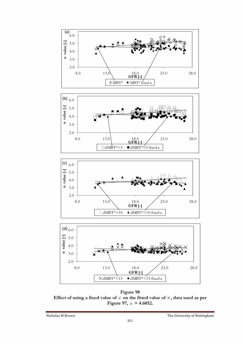
Nicholas M Brown The University of Nottingham
201
2.0
3.0
4.0
5.0
6.0
8.0 13.0 18.0 23.0 28.0
n v
alu
e [
-]
GFR [-]
MBT* MBT* fixed a
2.0
3.0
4.0
5.0
6.0
8.0 13.0 18.0 23.0 28.0
n v
alu
e [
-]
GFR [-]
dMBT*=5 dMBT*=5 fixed a
2.0
3.0
4.0
5.0
6.0
8.0 13.0 18.0 23.0 28.0
n v
alu
e [
-]
GFR [-]
dMBT*=10 dMBT*=10 fixed a
2.0
3.0
4.0
5.0
6.0
8.0 13.0 18.0 23.0 28.0
n v
alu
e [
-]
GFR [-]
dMBT*=15 dMBT*=15 fixed a
Figure 98 Effect of using a fixed value of a on the fitted value of n , data used as per
Figure 97, a = 4.6052.
(a)
(b)
(c)
(d)
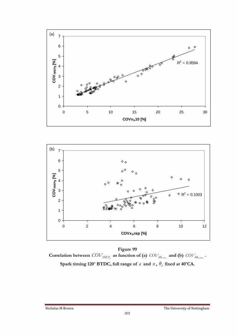
Nicholas M Brown The University of Nottingham
202
R2 = 0.9594
0
1
2
3
4
5
6
7
0 5 10 15 20 25 30
COVxb10 [%]
CO
VIM
EP
g [%
]
R2 = 0.1003
0
1
2
3
4
5
6
7
0 2 4 6 8 10 12
COVxbrap [%]
CO
VIM
EP
g [
%]
Figure 99
Correlation between gIMEPCOV as function of (a) 0 10%
COV and (b) 10 90%COV .
Spark timing 120o BTDC, full range of a and n , dq fixed at 40oCA.
(a)
(b)

Nicholas M Brown The University of Nottingham
203
0510
cov rba [%]
cov f
da [
%]
0 5 10 15 20 25 30 35 400
5
10
15
20
25
30
35
40
5
10
15
15
15
20
20
20
25
25
25
30
30
30
35
35
40
40
cov rba [%]
cov f
da [
%]
0 5 10 15 20 25 30 35 400
5
10
15
20
25
30
35
40
The effect of changes of 0 10%COV and 10 90%
COV on gIMEPCOV at five increasing dq :
(a) 30, (b) 50, (c) 70, (d) 90, (e) 115.
(a)
(b)

Nicholas M Brown The University of Nottingham
204
5
5
10
10
10
15
15
15
20
20
20
25
25
25
30
30
30
35
35
35
40
40
45
45
50
50
55
55
60
60
65 7075
80859095
cov rba [%]
cov f
da [
%]
0 5 10 15 20 25 30 35 400
5
10
15
20
25
30
35
40
0
0
0
5
5
5
10
10
10
15
15
15
20
20
20
25
25
25
30
30
30
35
35
35
40
40
45
45
50
50
55
55
60
60
65
7075
8085
9095100
cov f
da [
%]
cov rba [%]
0 5 10 15 20 25 30 35 400
5
10
15
20
25
30
35
40
The effect of changes of 0 10%COV and 10 90%
COV on gIMEPCOV at five increasing dq :
(a) 30, (b) 50, (c) 70, (d) 90, (e) 115.
(c)
(d)

Nicholas M Brown The University of Nottingham
205
15
15
20
20
20
25
25
25
30
30
30
35
35
35
40
40
40
45
45
45
50
50
50
55
55
55
60
60
60
65
65
65
70
70
70
75
75
75
80
80
85
85
90
90
95
95
100
100c
ov f
da [
%]
cov rba [%]
0 5 10 15 20 25 30 35 400
5
10
15
20
25
30
35
40
Figure 100
The effect of changes of 10bCOVx and 10 90%COV on
gIMEPCOV at five
increasing dq : (a) 30, (b) 50, (c) 70, (d) 90, (e) 115.
(e)