Brouwer and Euclid

Michael Beeson

July 18, 2017

Abstract

We explore the relationship between Brouwer’s intuitionistic mathe-matics and Euclidean geometry. Brouwer wrote a paper in 1949 called Thecontradictority of elementary geometry. In that paper, he showed that acertain classical consequence of the parallel postulate implies Markov’sprinciple, which he found intuitionistically unacceptable. But Euclid’sgeometry, having served as a beacon of clear and correct reasoning fortwo millennia, is not so easily discarded.

Brouwer started from a “theorem” that is not in Euclid, and requiresMarkov’s principle for its proof. That means that Brouwer’s paper did notaddress the question whether Euclid’s Elements really requires Markov’sprinciple. In this paper we show that there is a coherent theory of “non-Markovian Euclidean geometry.” We show in some detail that our theoryis an adequate formal rendering of (at least) Euclid’s Book I, and suf-fices to define geometric arithmetic, thus refining the author’s previousinvestigations (which include Markov’s principle as an axiom).

Philosophically, Brouwer’s proof that his version of the parallel pos-tulate implies Markov’s principle could be read just as well as geometricevidence for the truth of Markov’s principle, if one thinks the geometri-cal “intersection theorem” with which Brouwer started is geometricallyevident.

Contents

1 Introduction 2

2 Versions of the parallel postulate 42.1 Euclid’s parallel axiom . . . . . . . . . . . . . . . . . . . . . 52.2 Playfair’s axiom . . . . . . . . . . . . . . . . . . . . . . . . . 62.3 Brouwer’s intersection theorem . . . . . . . . . . . . . . . . 62.4 Euclid 5 formulated in Tarski’s language . . . . . . . . . . . 7

3 Constructive Euclidean geometry 73.1 Is Euclid constructive? . . . . . . . . . . . . . . . . . . . . . 73.2 The form of Euclid’s theorems and proofs . . . . . . . . . . 93.3 Euclidean geometry with Markov’s principle . . . . . . . . . 103.4 Angles and angle ordering . . . . . . . . . . . . . . . . . . . 11

1

4 Brouwer’s 1949 paper 124.1 What Brouwer actually proved . . . . . . . . . . . . . . . . 124.2 Implications of Brouwer’s theorem for

axiomatic geometry . . . . . . . . . . . . . . . . . . . . . . . 134.3 Why did Brouwer reject Markov’s principle? . . . . . . . . . 154.4 Two sides . . . . . . . . . . . . . . . . . . . . . . . . . . . . 16

5 Axioms of non-Markovian geometry 165.1 Markov’s principle and betweenness . . . . . . . . . . . . . 185.2 Distinct points and segment extension . . . . . . . . . . . . 195.3 The five-segment axiom and SAS . . . . . . . . . . . . . . . 215.4 Lines, rays, triangles, and right angles . . . . . . . . . . . . 225.5 Positive angles . . . . . . . . . . . . . . . . . . . . . . . . . 245.6 Non-Markovian inner Pasch . . . . . . . . . . . . . . . . . . 275.7 Non-Markovian outer Pasch . . . . . . . . . . . . . . . . . . 295.8 Line–circle and circle–circle continuity . . . . . . . . . . . . 305.9 Segment-circle continuity . . . . . . . . . . . . . . . . . . . 305.10 Dimension axioms . . . . . . . . . . . . . . . . . . . . . . . 315.11 List of axioms for reference . . . . . . . . . . . . . . . . . . 32

6 Development of non-Markovian geometry 346.1 Midpoints . . . . . . . . . . . . . . . . . . . . . . . . . . . . 356.2 Uniform perpendicular . . . . . . . . . . . . . . . . . . . . . 386.3 Euclid does not need Markov . . . . . . . . . . . . . . . . . 386.4 The exterior angle theorem and its consequences . . . . . . 396.5 Crossbar theorem . . . . . . . . . . . . . . . . . . . . . . . . 406.6 Further properties of angle ordering . . . . . . . . . . . . . 416.7 A lemma about two perpendiculars . . . . . . . . . . . . . . 426.8 Parallelograms . . . . . . . . . . . . . . . . . . . . . . . . . 436.9 Angle copying . . . . . . . . . . . . . . . . . . . . . . . . . . 446.10 Positive angles revisited . . . . . . . . . . . . . . . . . . . . 45

7 Geometric arithmetic without Markov’s principle 487.1 Coordinates . . . . . . . . . . . . . . . . . . . . . . . . . . . 487.2 Euclidean fields without Markov’s principle . . . . . . . . . 49

8 Geometric arithmetic 54

9 Some results about EG 549.1 A Kripke model of non-Markovian geometry . . . . . . . . . 549.2 EG is not too weak . . . . . . . . . . . . . . . . . . . . . . . 569.3 EG is strong enough . . . . . . . . . . . . . . . . . . . . . . 57

10 Conclusions 58

1 Introduction

Brouwer, in founding the philosophy of mathematics known as “intuition-ism”, rejected many of the mathematical results that were obtained in the

2

nineteenth century or before. The rejected body of mathematics has be-come known as “classical mathematics”. The word “classical” also bringsto mind the world of ancient Greece, where Euclid and his predecessorslaid the foundations of modern mathematical reasoning in the third cen-tury BCE. Euclidean geometry was for two millennia the sine qua non ofcareful reasoning; every educated person in Europe studied it; the Amer-ican Declaration of Independence was modeled on Euclidean reasoning.Brouwer did not directly challenge Euclid by name in any publication,but in 1949 he published a paper [7] with the title, Contradictority ofElementary Geometry.

Brouwer was never much of a diplomat. If his personality had beenmore diplomatic, he might have pointed out that, on a certain reading,certain theorems of elementary geometry related to the parallel postulatemay seem (intuitionistically) contradictory; but that every classical theo-rem permits various refinements, once constructive distinctions are takeninto account, and Euclid’s parallel postulate and its consequences are notexceptions.

What would Euclid have written, if he had come after Brouwer, insteadof before? Of course, he would not have thrown up his hands, thinkinggeometry is contradictory, and gone into investment banking instead. Wewill show in this paper that, if one is careful about the formulation ofthe axioms, Euclidean geometry is perfectly consistent with Brouwer’sintuitionism.

What Brouwer calls a “contradiction” has two parts: (i) Brouwer re-jects a certain property of the ordering of points on a line known asMarkov’s principle, and (ii) Brouwer shows that a certain “intersectiontheorem” (a classical consequence of Euclid’s parallel postulate) impliesMarkov’s principle, even though it appears not to imply the law of the ex-cluded middle. This result would be better summarized by the statement

Intuitionistic “elementary geometry” must distinguish betweendifferent propositions classically equivalent to Euclid’s parallelpostulate.

In previous work [4, 3], such distinctions were made, and a coherenttheory of constructive geometry developed. But that theory would nothave met with Brouwer’s approval, because Markov’s principle is assumedas an axiom. The reason for that was simple pragmatism: it enables oneto argue by contradiction and cases, as long as one is trying to provebetweenness and congruence assertions about specific points, rather thanassertions that more points exist with certain properties.1

Thus, the door is open (and has been open for 68 years) for a de-velopment of Euclidean geometry that explicitly avoids not only the lawof the excluded middle, but also Markov’s principle. We call this theory“non-Markovian Euclidean geometry”, or for short just “non-Markoviangeometry.” Perhaps it should be called “intuitionistic geometry”, if onefeels that the rejection of Markov’s principle is fundamental to intuition-ism.

1For logicians: allowing Markov’s principle enabled the double negation interpretation towork, allowing the “importation” of a certain class of geometrical results, whose classicalproofs are long and complicated.

3

The key concepts of non-Markovian geometry are the concepts of “dis-tinct points” and “positive angles.” The concept that a and b are distinctis written a#b, and is stronger than simple inequality a 6= b. Intuitively,a#b means that we have a positive lower bound on how far apart a and bare, although in axiomatic geometry there is of course no notion of “dis-tance.” The concept that angle abc is “positive”, written 0 < abc, meansintuitively that we have a lower bound on how different the directions ofthe rays bc and ba are.

Both these concepts will be defined in terms of betweenness and con-gruence, rather than be introduced as primitive. In particular the correctdefinition of “positive angle” is not obvious a priori. In order to ensurethat the axioms do not imply Markov’s principle immediately, Pasch’s ax-iom must be restricted to assume that certain angles are positive. Thenthe definition of “positive angle” must be broad enough to permit the ap-plications of Pasch that are needed to “bootstrap” geometry. But finally,we should be able to prove that a positive angle is simply the apex angleof an isosceles triangle (whose three points are distinct). Then EuclidBook I can be proved, when angles are assumed to be positive (and havepositive supplements) and triangles, by definition of “triangle”, have dis-tinct vertices. In the last section we give a metamathematical theorem tothe effect that this claim can be extended to (at least) Books II and IIIas well.2

There have been some papers on related subjects in the seven decadessince Brouwer’s rejection of “elementary geometry”, and the obligationarises to explain in what relation the present work stands to those papers.Almost all of those papers were about projective geometry, or affine geom-etry, or Desarguesian geometry, rather than Euclidean geometry, and alsowere based on (or included) apartness, which is rejected in this work. Hereis a brief, possibly incomplete, list of such papers. The first was Heyting’s1925 thesis (published two years later as [12] and again 34 years later as[13].) Heyting’s student van Dalen continued work on intuitionistic pro-jective spaces in [30, 31, 32]; see also [34] and [20, 21, 23, 22]. Aside fromthe previous work of the present author [3, 5], the only previous paper onconstructive Euclidean geometry was by Lombard and Vesley [19], whofollowed Heyting in taking apartness as primitive.

2 Versions of the parallel postulate

The “parallel postulate” of Euclid has been reformulated many times inthe history of geometry, as efforts to prove it led instead to many differentequivalent propositions. But not all these versions are equivalent usingintuitionistic logic. Euclid’s version requires two lines to meet, if twospecified angles “make less than two right angles.” A different version dueto the Englishman Playfair (1729), was popularized by Hilbert; it assertsthe impossibility of two different lines parallel to a given line through thesame point. In so doing it makes no existential assertion, unlike Euclid’sversion, which asserts the existence of an intersection point.

2This claim cannot be taken too literally, as of course Euclid does contain gaps and errors.

4

In this section, we will review several versions of the parallel postulate,and then discuss Brouwer’s 1949 proof. All these versions of the parallelpostulate, including Euclid’s own, are consistent with intuitionistic logic.Brouwer’s paper shows that his version of the parallel postulate impliesa certain ordering principle, known as Markov’s principle, which Brouwerbelieved to be contrary to the nature of the intuitionistic continuum, forreasons far removed from Euclidean geometry.

2.1 Euclid’s parallel axiom

Euclid’s postulate 5 is

If a straight line falling on two straight lines make the interiorangles on the same side less than two right angles, the twostraight lines, if produced indefinitely, meet on that side onwhich are the angles less than the two right angles.

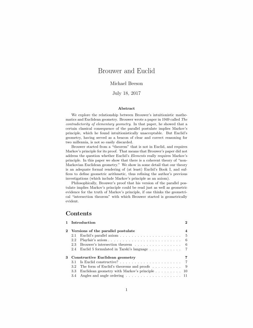
We consider the formal expression of Euclid’s parallel axiom. Let Land M be two straight lines, and let pq be the “straight line falling on”L and M , with p on M and q on L. We think that what Euclid meantby “makes the interior angles on the same side less than two right angles”was that, if K is another line through p, making the interior angles withpq equal to two right angles, then M would lie in the interior of one ofthose interior angles (see Fig. 1).

Euclid did not define “angle”, and did not define “lies in the interior ofan angle”, but these issues of precision have little to do with intuitionism.Assuming for the moment that we understand the notions of “angle” and“alternate interior angle”, then we can state Euclid’s parallel axiom, usingthree more points to “witness” that one ray of line M emanating from plies in the interior of one of the interior angles made byK. Fig. 1 illustratesthe postulate. The point asserted to exist is shown by a small open circle(a convention we will follow throughout).

bp

b

a

b

q

br

L

K

M

Figure 1: Euclid 5: M and L must meet on the right side, pro-vided B(q, a, r) and pq makes alternate interior angles equal withK and L.

In this formulation, the point is asserted to exist “on the right side”;more precisely, “on the same side of pq as a.” Euclid did not define “onthe same side of”, although his postulate uses that phrase. That notionwas, apparently, first defined by M. Pasch in 1882 (on page 27 of [25]).

5

2.2 Playfair’s axiom

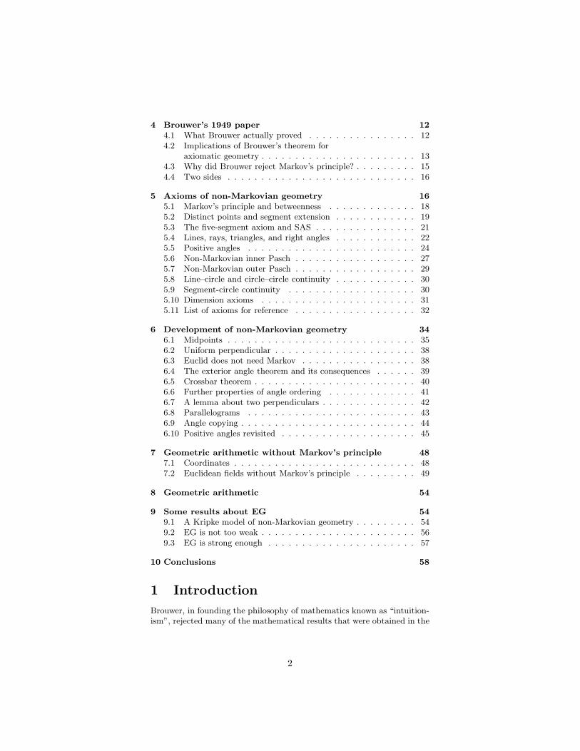
“Playfair’s axiom” is the version of the parallel axiom adopted by Hilbertin [15]. That version, unlike all the other versions, makes no existenceassertion at all, but only asserts that there cannot exist two different linesparallel to a given line through a given point.

bp

L

K

M

Figure 2: Playfair: if K and L are parallel, M and L are notparallel.

The conclusion of Playfair’s axiom is that M and L are not parallel. Bydefinition, parallel lines are lines that do not meet, so the conclusion is thatM and L cannot fail to meet. That is, not not there exists an intersectionpoint. Since ¬¬∃ is equivalent to ¬∀¬, no existential quantifier is neededto express Playfair’s axiom.

2.3 Brouwer’s intersection theorem

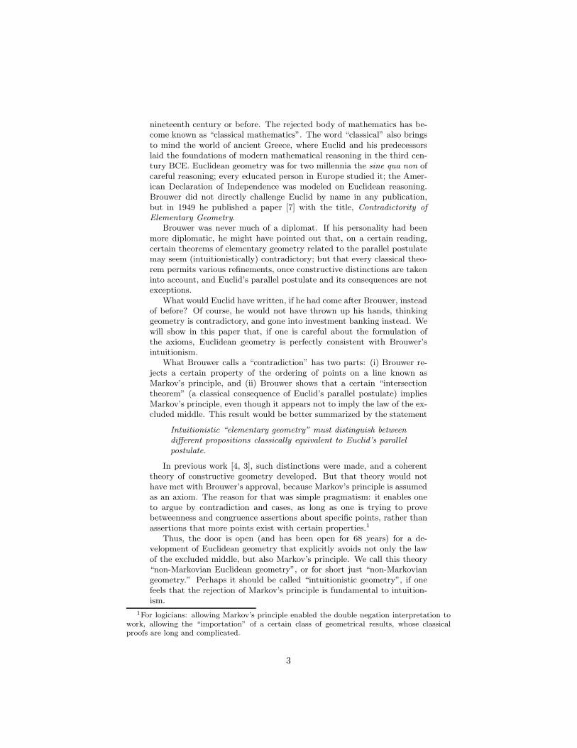
Brouwer considers a version of the parallel postulate similar to Euclid’s,but without the “witness” a in the hypothesis testifying to the side onwhich the angles are less than a right angle. It is similar to a variant ofPlayfair’s axiom in which “M and L cannot fail to meet” is replaced by“M and L meet.” Rather than calling it a “postulate”, Brouwer refers tothe “intersection theorem of Euclidean plane geometry”, which he statesas “a common point can be found for any two lines a and ℓ in the Euclideanplane which can neither coincide nor be parallel.” See Fig. 3.

bp

b

q

br

L

K

M

Figure 3: Brouwer’s intersection theorem: M and L must meet,provided pq makes alternate interior angles equal with K and L.

This version of the parallel postulate was rediscovered (or re-invented?)in [2, 4], where it was called the “strong parallel postulate.” There it was

6

introduced in an axiomatic setting that included the stability of between-ness, or Markov’s principle. As we shall discuss below, this version of theparallel postulate, in the absence of Markov’s principle, needs a strongerhypothesis to make constructive sense: he should have required that Mand K make a positive angle, i.e., are “positively non-collinear”. Withoutthat hypothesis, it is hardly surprising that Brouwer’s intersection the-orem implies Markov’s principle, for the hypothesis that M and K areunequal lines is a negative one, but the conclusion that M meets L is apositive one.

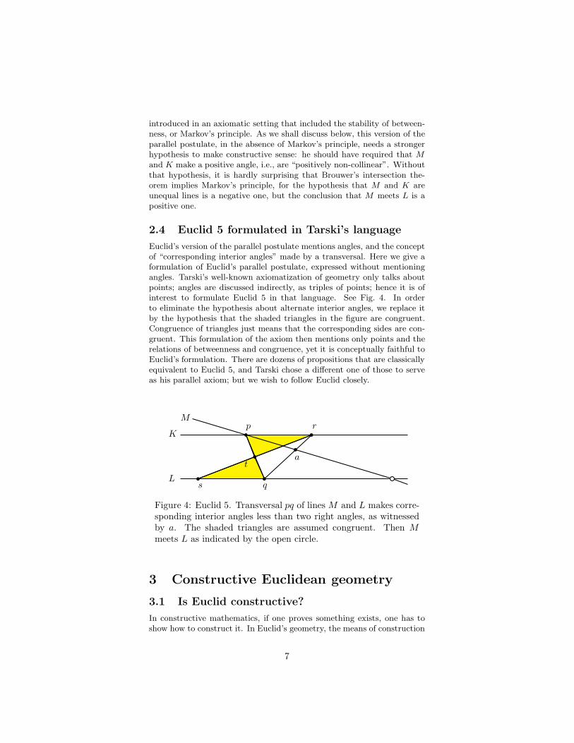
2.4 Euclid 5 formulated in Tarski’s language

Euclid’s version of the parallel postulate mentions angles, and the conceptof “corresponding interior angles” made by a transversal. Here we give aformulation of Euclid’s parallel postulate, expressed without mentioningangles. Tarski’s well-known axiomatization of geometry only talks aboutpoints; angles are discussed indirectly, as triples of points; hence it is ofinterest to formulate Euclid 5 in that language. See Fig. 4. In orderto eliminate the hypothesis about alternate interior angles, we replace itby the hypothesis that the shaded triangles in the figure are congruent.Congruence of triangles just means that the corresponding sides are con-gruent. This formulation of the axiom then mentions only points and therelations of betweenness and congruence, yet it is conceptually faithful toEuclid’s formulation. There are dozens of propositions that are classicallyequivalent to Euclid 5, and Tarski chose a different one of those to serveas his parallel axiom; but we wish to follow Euclid closely.

bp

b

a

b

qb

s

br

b

t

L

K

M

Figure 4: Euclid 5. Transversal pq of lines M and L makes corre-sponding interior angles less than two right angles, as witnessedby a. The shaded triangles are assumed congruent. Then M

meets L as indicated by the open circle.

3 Constructive Euclidean geometry

3.1 Is Euclid constructive?

In constructive mathematics, if one proves something exists, one has toshow how to construct it. In Euclid’s geometry, the means of construction

7

are not arbitrary computer programs, but ruler and compass. Therefore itis natural to look for quantifier-free axioms, with function symbols for thebasic ruler-and-compass constructions. The terms of such a theory cor-respond to ruler-and-compass constructions. These constructions shoulddepend continuously on parameters, since we want to allow an interpre-tation of geometry in which the points are given by successive approxi-mations. We can see the continuity of ruler-and-compass constructionsdramatically in computer animations, in which one can select some of theoriginal points and drag them, and the entire construction “follows along.”We expect that if one constructively proves that points forming a certainconfiguration exist, then the construction can be done “uniformly”, i.e.,by a single construction depending continuously on parameters.

To illustrate what we mean by a uniform construction, we consider animportant example. There are two well-known classical constructions forconstructing a perpendicular to line L through point p: one of them iscalled “dropping a perpendicular”, and works when p is not on L. Theother is called “erecting a perpendicular”, and works when p is on L.Classically we may argue by cases and conclude that for every p and L,there exists a perpendicular to L through p. But constructively, we arenot allowed to argue by cases. If we want to prove that for every p and L,there exists a perpendicular to L through p, then we must give a single,“uniform” ruler-and-compass construction that works for any p, whetheror not p is on L.

The other type of argument (besides argument by cases) that is fa-mously not allowed in constructive mathematics is proof by contradiction.There are some common points of confusion about this restriction. Themain thing one is not allowed to do is to prove an existential statement bycontradiction. For example, we are not allowed to prove that there existsa perpendicular to L through x by assuming there is none, and reachinga contradiction. From the constructive point of view, that proof of courseproves something, but that something is weaker than existence. We writeit ¬¬∃, and constructively, one cannot delete the two negation signs.

However, when proof by contradiction is used only to prove that twopoints are equal, or two segments are congruent, or that one point is be-tween two others, the situation seems qualitatively different. There is no“existential information” missing from such a proof. Nothing is being as-serted to exist, let alone being asserted to exist without being constructed.The question then arises, whether such proofs are constructively accept-able. That is, whether one is or one is not allowed to prove equalities,congruences, and inequality or order relations between points by contra-diction. Consider for the moment two points x and y on a line. If wederive a contradiction from the assumption x 6= y, then x = y. Formallythis becomes the implication

¬x 6= y → x = y.

In the style of Euclid: Things that are not unequal are equal. It has itsintuitive grounding in the idea that x = y does not make any existentialstatement. This principle is named “the stability of equality.” (Generallyany relation is “stable” if it is implied by its double negation.)

8

The principle that x < y can be proved by contradiction can be ex-pressed by

¬¬ x < y → x < y.

or equivalently¬ y ≤ x→ x < y.

Since order on a line is not a primitive relation in geometry, we considerinstead the corresponding axiom for the betweenness relation, namely

¬¬B(a, b, c) → B(a, b, c).

This is known as “the stability of betweenness.” It is also known as“Markov’s principle”, since it was adopted by Markov as a basic principleof Russian constructive mathematics.

Here is a geometric way of thinking about Markov’s principle, ratherthan as a principle about ordering the continuum. Markov’s principlereduces to the assertion that, given two points s and t, we can find twocircles with centers s and t that separate the two points. The obviouscandidate for the radius is half the distance between s and t, so the ques-tion boils down to Markov’s principle for numbers: if that radius is notnot positive, must it be positive? The stability of betweenness thus hasthe same philosophical status as Markov’s principle: it is self-justifying,not provable from other constructive axioms, and leads to no trouble inconstructive mathematics, while simplifying many proofs.

Brouwer was not a person to accept a principle because it was useful,convenient, and apparently harmless, in the sense that it does not interferewith the constructibility of solutions proved to exist with its aid. BeforeBrouwer would accept a principle, he wanted it to be true, and he saw noreason why Markov’s principle has to be true.

3.2 The form of Euclid’s theorems and proofs

It is helpful to remember that Euclid did not work in first-order logic. Histheorems, and their proofs, have a fairly simple structure: Given somepoints, lines, and circles bearing certain relations, then there exist somefurther points bearing certain relations to each other and the originalpoints. This logical simplicity implies that (although this may not beobvious at first consideration) if we allow the stability axioms for equalityand betweenness, then essentially the only differences between classicaland constructive geometry are the two requirements:

• You may not prove existence statements by contradiction; you mustprovide a construction.

• The construction you provide must be uniform; that is, it must beproved to work without an argument by cases.

Sometimes, when doing constructive mathematics, one may use a men-tal picture in which one imagines a point p as having a not-quite-yet-determined location. For example, think of a point p which is very closeto line L. We may turn up our microscope and we still can’t see whetherp is or is not on L. We think “we do not know whether p is on L or not.”Our construction of a perpendicular must be visualized to work on such

9

points p. Of course, this is just a mental picture and is not used in actualproofs. It can be thought of as a way of conceptualizing “we do not havean algorithm for determining whether p is on L or not.”

We illustrate these principles with a second example. Consider theproblem of finding the reflection of point p in line L. Once we know howto construct a perpendicular to L through p, it is still not trivial to findthe reflection of p in L. Of course, if p is on L, then it is its own reflection,and if p is not on L, then we can just drop a perpendicular to L, meetingL at the foot f , and extend the segment pf an equal length on the otherside of f to get the reflection. But what about the case when we do notknow whether p is or is not on L? Of course, that sentence technicallymakes no sense; but it illustrates the point that we are not allowed toargue by cases. The solution to this problem may not be immediatelyobvious; see [4].

The description given above of the form of Euclid’s theorems is sup-ported by Avigad et. al. in [1]:

Euclidean proofs do little more than introduce objects satisfy-ing lists of atomic (or negation atomic) assertions, and thendraw further atomic (or negation atomic) conclusions fromthese, in a simple linear fashion. There are two minor depar-tures from this pattern. Sometimes a Euclidean proof involvesa case split; for example, if ab and cd are unequal segments,then one is longer than the other, and one can argue that adesired conclusion follows in either case. The other exceptionis that Euclid sometimes uses a reductio; for example, if thesupposition that ab and cd are unequal yields a contradictionthen one can conclude that ab and cd are equal.

These arguments are constructively acceptable, if we have the stabilityof congruence and betweenness. In [4], several examples such argumentsin Euclid are examined, including I.6 and I.24. If the conclusion is acongruence or equality statement, even an argument based on “of twounequal segments, one is longer than the other” does not require Markov’sprinciple, but only the stability of congruence.

3.3 Euclidean geometry with Markov’s principle

In [4], I advocated adopting the stability of equality, congruence, and be-tweenness as axioms of constructive geometry. In particular, I argued thatEuclid Books I-IV can be formalized using intuitionistic logic plus thosetwo stability principles, using Euclid’s version of the parallel postulate in-stead of Hilbert’s, and otherwise making no changes in Hilbert’s axioms.In [3], a version of constructive Euclidean geometry is given that is basedon Tarski’s language and axioms, slightly modified. In addition to usingEuclid 5 instead of Tarski’s parallel axiom, we found it necessary to usestrict betweenness. Hilbert used strict betweenness, but Tarski used non-strict betweenness. To avoid confusion, in this paper we use B(a, b, c) forstrict betweenness and T(a, b, c) for non-strict betweenness (T being thefirst initial of “Tarski”). For details of the axioms see [3]; the essentialidea is that after replacing T by B, we have to “put back” some axioms

10

that Tarski originally used, but later found clever derivations of from theremaining axioms, using in an essential way the “degenerate cases” ofthose axioms where non-strict betweenness holds.

In these two long papers, I showed that Euclid 5 together with thestability of congruence and betweenness allows the formalization, not onlyof Euclid Books I–IV, but also of the construction of coordinates, so thatone can construct within geometry the field operations defined on a fixedline L (taken as the x-axis).

The consistency of Euclidean geometry with stability axioms, at leastrelative to classical Euclidean geometry, is obvious, since all the axiomsare classically valid. It may be more instructive to note that Euclideangeometry also has a model in the recursive reals, i.e. those real numbersgiven by recursive Cauchy sequences with a specified rate of convergence.This model can be formalized in arithmetic, and the resulting interpre-tation is, using standard recursive realizability, consistent with Markov’sprinciple and Church’s thesis for arithmetic. Thus, also in the sense ofrecursive mathematics, there is nothing inconsistent about the stability ofequality and betweenness.

Julien Narboux pointed out that the stability of equality can be derivedfrom the stability of congruence. The proof is given, in the context ofTarski’s theories, in Lemma 7.1 of [4]. The converse is also easy to prove.So there are really only two stability axioms to consider: stability ofcongruence and stability of betweenness.

3.4 Angles and angle ordering

As is well-known, betweenness is never explicitly mentioned in Euclid.There are three ways that betweenness occurs implicitly in the statementsof Euclid’s propositions: collinearity, ordering of segments, and orderingof angles. Euclid takes these concepts as undefined, and assumes (inthe common notions) the basic properties of ordering. Hilbert also tookangles and congruence of angles as primitive notions, but unlike Euclid,he defined angle ordering. Tarski defined all three notions. The basicproperties of angle ordering then become theorems. These developmentsare spelled out in [26], Chapter 11, with attention to constructivity in [3],§8.11. We here review that treatment to see whether and where Markov’sprinciple was used.

The concept “x lies on Ray(b, a)” is needed to define angles. In[3] §8.11, we defined “x lies on Ray(b, a)” by ¬(¬T(b, x, a)∧¬T(b, a, x)).Here T is non-strict betweenness. That definition will not do if we do nothave Markov’s principle. Instead, we should use the definition

∃e (B(e, b, x) ∧B(e, b, a) ∧ eb = ea).

That is, x is on the opposite side of b from the reflection e of a in b. Inparticular, the reflection e must exist for x to be on the ray. Of course, ifwe assume Markov’s principle, then the two definitions are equivalent.

Then “abc and ABC are the same angle” means that the same pointslie on Ray(b, a) as on Ray(B,A) and the same points lie on Ray(b, c) as onRay(B,C). Then two angles abc and ABC are congruent if by changing

11

a, c, A, and C to other points on those same rays, we can make ab = ABand bc = BC and ac = AC.

We say “f lies in the interior of angle abc if there is a “crossbar” uv,with u on Ray(b, a) and v on Ray(b, c), with u, b, and v distinct, andfor some point e we have B(u, e, v) and B(b, e, f). Then if f lies in theinterior of abc, it also lies in the interior of any a′bc′ that is the “sameangle” as abc.

4 Brouwer’s 1949 paper

4.1 What Brouwer actually proved

What did Brouwer mean by asserting the inconsistency of Euclidean geom-etry? In this section we answer that question. Brouwer worked extensivelywith “the continuum”, which we denote here by R. We refer to membersof the continuum as “real numbers”, rather than using Brouwer’s termi-nologies for numbers given by certain kinds of sequences. Geometry hasa model in which the points are pairs of real numbers (x, y). We refer tothis model as “the model R2.”

Real numbers are given by sequences of rationals, and order in R isdefined in terms of order in the rationals and the concept of sequence, soit implicitly depends on the natural numbers. Order in geometry, on theother hand, is defined in terms of betweenness on a line, which in turn isgiven by some axioms about betweenness. In Brouwer’s 1949 paper, he isconcerned only with the model R2 of geometry, and not with axiomaticgeometry.

Here is what Brouwer proved in [7]:

Theorem 1 (Brouwer) In the model R2, the statement “the strong par-allel postulate implies Markov’s principle” holds.

Proof. Let L be the x-axis and P be the point (0, 1). Assume ¬¬ ǫ > 0.Let a = (1, 1 − ǫ). According to the strong parallel principle, the linethrough P and a meets L. The point of intersection is (x, 0), where bysimilar triangles x is to 1 as 1 is to ǫ. (The existence of x is guaranteedby the strong parallel postulate, not by division by ǫ, which would notbe legal under the weak assumption ǫ 6= 0.) Now Brouwer appeals to thefact that R satisfies the Archimedean axiom: there is a positive integerN , which Brouwer chooses in the form 2nℓ , greater than |x|. Now wehave x < N , and both sides of the inequality have multiplicative inverses.Brouwer says (line 12 of his paper, where his ρℓ is our −ǫ)

ρℓ < −2−nℓ

or in our notation,

ǫ >1

N.

Brouwer offers no further justification, but we think some is necessary.Now ǫ = 1/x, so to justify Brouwer’s conclusion we would need to infer1/x > 1/N from x < N and the existence of 1/x and 1/N . We know

12

N > 0, but we only know ¬¬ x > 0; hence we do not know xN > 0 andthe last step of the following argument cannot be carried out

1

x− 1

N=N − x

xN> 0

since the last step would require xN > 0, which we do not have. Instead,we get only

¬¬ ǫ >1

N.

We can, however, justify Brouwer’s argument using apartness. The prin-ciple of apartness, which holds in R

2, says that if α < β, then

z < β ∨ α < z.

It follows that if α > 0 and ¬¬ β > 0, then α+β > 0, since by apartness,α + β > 0 ∨ α + β < α, and the second case, α + β < α, implies β < 0,which contradicts ¬¬ β > 0. Applying this principle with β = 1/x− 1/Nand α = 1/2N , we have

1

x− 1

N+

1

2N=

1

x− 1

2N> 0

and hence ǫ > 1/2N > 0 as desired. That completes the proof.

Brouwer used the Archimedean axiom to get a positive upper boundon x. That is not necessary, and neither is the use of apartness. We nowshow how to remove these two principles from Brouwer’s proof. First, weobserve that from the hypothesis ¬¬ ǫ > 0 and the equation x = 1/ǫ, wehave ¬¬ x > 0. From ¬¬ x > 0 we have ¬¬ x = |x|. By the stability ofequality, we have x = |x|.

Now, instead of using Archimedes’s axiom to get a positive upperbound on x, we could just as well use |x|+ 1. Then we have

0 <1

2(|x|+ 1)<

1

|x| =1

x= ǫ

and hence ǫ > 0. The use of Archimedes’s axiom is a red herring (for thisproof—not necessarily in general for intuitionism). That Brouwer usedit anyway shows how far from Brouwer’s mind was any consideration ofwhether his argument was first-order or not.

4.2 Implications of Brouwer’s theorem for

axiomatic geometry

Brouwer’s theorem is formulated as a theorem about the Euclidean planeR

2. But for half a century already at the time of Brouwer’s publication,ever since Hilbert’s 1899 book [15], geometry had moved on from dis-cussing the one true plane to axiomatic formulations. In Brouwer’s paper,he did not consider the question whether Markov’s principle is contradic-tory in some axiomatic system for Euclidean geometry. That may havebeen because of his aversion to axiomatics in general, or it may have beenthe lack of any development at all of constructive Euclidean geometry at

13

that time, or it may have been for some other reason entirely. But now,the question seems natural.3 Can we use Brouwer’s proof to show thatthe axioms of Euclidean geometry (as formulated for example in [3], butwithout Markov’s principle) allow one to deduce Markov’s principle fromBrouwer’s version of the parallel axiom?

We showed above that Brouwer’s use of the Archimedean axiom andhis (implicit) use of apartness are easily eliminated. The one remainingissue is his use of coordinate geometry. What Brouwer’s proof shows isthat, if some theory of Euclidean geometry suffices to define coordinatesand arithmetic, then in that theory, Brouwer’s version of the parallel pos-tulate implies Markov’s principle. That is, after all, not too surprising,given that the hypothesis of Brouwer’s “intersection theorem” is the neg-ative statement that the two lines M and K are not identical, but theconclusion is a positive existence statement. Markov’s principle is “built-in.”

Later in this paper, we will give a formal theory EG for Euclideangeometry without Markov’s principle. The theory EG plus Markov’s prin-ciple has been extensively studied in [3, 4]. The fact that an attractivetheory of geometry can be formulated without using Markov’s principleas an axiom, and without any obvious way to prove Markov’s principle,leads to the following questions and conclusions:

(1) Does EG (which does not have MP) plus Euclid 5 suffice to definecoordinates and geometric arithmetic? For short we say “EG can definearithmetic” to describe this property. We claim in this paper that EG candefine arithmetic.

(2) Then Brouwer’s proof shows that EG plus Brouwer’s intersectiontheorem proves MP.

(3) We know [4] that EG + MP proves Brouwer’s intersection theorem,which is there called the “strong parallel postulate”, or SPP for short.Hence SPP is actually equivalent to MP in EG.

HA is “Heyting’s arithmetic”, the standard formal theory of arithmeticwith intuitionistic logic. In the context of HA, “Markov’s principle” is thename usually given to

¬¬∃xP → ∃xP (P primitive recursive).

It is well-known (see e.g. [29]) that this principle is not provable inHA. Consider the interpretation of EG in HA determined by representingpoints as pairs of (indices of) recursive real numbers. To verify that theinterpretations of the axioms of EG are provable in HA, we do not needMarkov’s principle, since the stability of betweenness is not an axiom ofEG. We also do not need Markov’s principle to verify any of the otheraxioms of EG, including Euclid 5, since the coordinates of the point as-serted to exist by Euclid 5 involve only positive denominators. To show

3The referee pointed out that Brouwer was the thesis advisor, two years after the publica-tion of the article on the contradictority of elementary geometry, of Johanna Adriana Geldof’sthesis [9]. This thesis has nothing specifically intuitionistic in it, except one sentence near thebeginning saying that it assumes any two elements are either equal or not equal, and alsonothing specifically Euclidean, but it does show that Brouwer’s aversion to axiomatics wasnot absolute.

14

that EG does not prove the geometric Markov’s principle (stability of be-tweenness) it therefore suffices to prove that the recursive interpretation ofthe geometric Markov’s principle is equivalent to the arithmetic Markov’sprinciple. But that is an easy exercise. Hence

(4) EG does not prove Markov’s principle.

Since Brouwer’s “intersection theorem” is equivalent to Markov’s prin-ciple, EG does not prove that “theorem.” In particular Brouwer’s “inter-section theorem” is not verifiable in the recursive interpretation (unlesswe assume the arithmetic Markov principle).

Brouwer never mentioned (in the paper under consideration, or any-where else as far as I know) Euclid, or Euclid’s axioms; nor did he men-tion Hilbert, or Hilbert’s axioms, or any axiomatic system whatever. Heworked simply with the plane R

2 using coordinate geometry. He showedthat if R2 satisfies the “intersection theorem”, then R satisfies Markov’sprinciple. The title of his paper, however, claims that “elementary ge-ometry is contradictory.” To reach that conclusion from his result, onewould need to believe that the intersection theorem is part of elemen-tary geometry, and that Markov’s principle is contradictory. Of coursethe intersection theorem is a part of classical elementary geometry, butits proof requires Markov’s principle, so it is not a part of intuitionisticelementary geometry, unless one assumes Markov’s principle or an axiomthat implies Markov’s principle. In particular, the intersection theoremin question does not follow from Euclid’s formulation of the parallel pos-tulate.

4.3 Why did Brouwer reject Markov’s principle?

Brouwer had claimed in that same year (1949) in [8] that Markov’s prin-ciple is contradictory. His proof used real numbers that are limits ofsequences generated by the “creative subject”, who is allowed to examineat each stage of mathematical construction, all proofs developed at earlierstages. Brouwer regarded this as an improvement over a paper publishedthe previous year [6], in which he showed that Markov’s principle was“unlikely to be provable.” In view of these results, Brouwer viewed hisversion of the parallel axiom as “contradictory.”

Here is a sketch of Brouwer’s refutation of MP, in more modern terms.He used Kripke’s schema (KS), according to which any proposition φ isequivalent to a proposition of the form α > 0, for some real number α.Taking φ to be A ∨¬A, and noting that ¬¬ (A∨¬A) is intuitionisticallyvalid, we have ¬¬ α > 0, so by Markov’s principle α > 0; that is, A∨¬A.Hence KS implies the law of the excluded middle. But the fan theorem(uniform continuity of functions on 2N ) refutes the law of the excludedmiddle. Hence KS plus the fan theorem refutes MP. Brouwer believed, atthe time of writing the papers we are discussing, that his theory of thecreative subject justified KS, and hence, that MP had been refuted.

Krike’s schema has found few (if any) adherents in the 70 years sinceBrouwer advocated it. On the other hand, Markov’s principle is consistentwith most commonly-studied intuitionistic theories; in particular with thetheories of intuitionistic analysis including Brouwer’s fan theorem and bar

15

theorem as axioms. See [28] and [18] for proofs of this consistency usingvariations of recursive realizability.

4.4 Two sides

In Brouwer’s paper [7], he also considered an ordering principle that wecall “two-sides”:

x 6= 0 → x < 0 ∨ x > 0.

The name is chosen because the principle can be thought of as saying thatthere are “two sides” of the y-axis: every point not on the y-axis lies onthe left half of the plane or on the right half.

We digress to show that two-sides can be expressed in the language ofgeometry. Fix two points 0 and 1, and define −1 to be the endpoint ofthe extension of the line segment from 1 to 0 by itself. Then x < 0 canbe defined as B(x, 0, 1). Two-sides can be expressed as

x 6= 0 → B(x, 0, 1) ∨B(−1, 0, x).

Brouwer rejected not only Markov’s principle, but also two-sides. Two-sides is not a theorem of EG, even with the help of Markov’s principle,as shown in [3]. Proof sketch: the axioms of EG can be expressed, afterintroducing some function symbols, without using ∃ or ∨. Then cut-elimination can be used to show that no disjunctive theorems can beproved (unless one of the disjuncts can be proved.) Two-sides does implyMarkov’s principle, since if we assume ¬¬ x > 0, then x 6= 0, so by two-sides, x > 0∨x < 0; but x < 0 contradicts ¬¬ x > 0, so that case is ruledout, and we conclude x > 0. Thus two-sides is stronger than Markov’sprinciple.

5 Axioms of non-Markovian geometry

Brouwer’s objection to Markov’s principle led us to consider whetherMarkov’s principle is really necessary for Euclidean geometry. In thispaper, we introduce a theory EG of Euclidean geometry, with the stabil-ity of congruence (and hence the stability of equality) but without thestability of betweenness (which is also called Markov’s principle). EG hasEuclid 5 for its parallel postulate, so it corresponds closely to Euclid. Theaxioms of EG are listed for reference in §5.11, but we shall introduce themgradually, with explanations.

It probably does not matter whether we take a Hilbert-type formula-tion or a Tarski-type formulation as in [3], but for the sake of precision wemust pick a specific list of axioms, and it is far simpler to work with thesimple language and short list of axioms of Tarski’s theory. As a start-ing point, we consider the constructive version of Tarski’s axioms givenin [3], with Markov’s principle deleted from the list of axioms. We alsoneed to modify two other axioms (segment extension and Pasch) to ensurethat they do not immediately imply Markov’s principle. We postpone thedetails of those modifications of the axioms to the next two sections.

16

EG has line–circle continuity: a line through a point (strictly) inside acircle meets the circle in two distinct points. We also include circle–circlecontinuity as an axiom.4

What we seek, then, is an axiomatization of EG such that each axiomis equivalent (using MP) to an axiom of intuitionistic Tarski geometry (asdefined in [3]), such that EG does not imply Markov’s principle, and yetsuffices for the development of Euclidean geometry. More specifically, wewant EG to satisfy these criteria:

• EG suffices to prove the correctness of the uniform constructionsgiven in [3], namely, uniform perpendicular and reflection in a point.This permits the assignment of coordinates (x, y) to each point, giventwo fixed perpendicular lines to serve as the x-axis and y-axis.

• EG suffices to prove that every pair (x, y) occurs as the coordinatesof some (unique) point.

• EG suffices to define the (uniform) addition and multiplication of(signed) points on the x-axis, and the construction of square rootsof non-negative points.

• EG suffices to formalize the arguments of Euclid Book I, and prob-ably Books II–IV as well.

The papers [3] and [4] established these facts for a theory includingMarkov’s principle, so the task here is to find a modified version of thistheory that does not imply Markov’s principle but still satisfies the criterialisted above.

In particular, we give EG the parallel axiom Euclid 5 (just as in [4, 3]rather than the “strong parallel axiom” used by Brouwer. It follows that,in some sense, Brouwer was criticizing a “straw man”, in that the parallelpostulate that he found unsatisfactory is not actually Euclid’s parallelpostulate, and Euclid 5 does not suffer from the flaw (if it is a flaw)that Brouwer pointed out. The strong parallel postulate and Euclid 5 areequivalent in Euclidean geometry with Markov’s principle (as shown in[4]), but they are not equivalent if Markov’s principle is dropped, since(at least with the aid of the apartness axioms) the strong parallel postulateimplies Markov’s principle, while Euclid 5 does not.

There is no philosophical advantage (for the present purposes) in tryingto choose a minimal set of axioms for EG, and indeed there are reasons(discussed below) to be generous in taking more axioms than probablyare necessary. We assume two versions of Pasch, and both line–circle andcircle–circle continuity. We modify Pasch’s axioms to avoid degeneraciesthat imply discontinuous dependence (as we did in [3]) and also to avoidnear-degeneracies that imply Markov’s principle. The remarkable con-clusion is that we can then derive Euclid Book I (and probably II-IV),coordinates, and arithmetic, without Markov’s principle, though we doneed to add hypotheses that angles are positive and vertices are distinct.

4For our present purposes, there is little to be gained by trying to eliminate circle–circlecontinuity as an axiom, or in general, by trying to minimize the number of axioms, sinceour aim is simply to demonstrate the viability of intuitionistic geometry without Markov’sprinciple.

17

5.1 Markov’s principle and betweenness

Tarski’s geometry, and its variant EG, include a minimal set of axiomsabout betweenness. Remember that we use strict betweenness B ratherthan non-strict betweenness T as in Tarski. If we have Markov’s principle,then B and T are interdefinable. But without Markov’s principle, thereis no apparent way to define B from T, so it is good that we took B asfundamental.

Tarski’s final theory [27] had only one betweenness axiom, known as(A6) or “the identity axiom for betweenness”:

T(a, b, a) → a = b.

In terms of strict betweenness, that becomes ¬B(a, x, a), or otherwiseexpressed, B(a, b, c) → a 6= c. We also refer to this axiom as (A6). Theoriginal version of Tarski’s theory had more betweenness axioms (see [27],p. 188). These were all shown eventually to be superfluous in classicalTarski geometry, through the work of Eva Kallin, Scott Taylor, Tarskihimself, and especially Tarski’s student H. N. Gupta [11]. These proofsappear in [26]. Here we give the axiom numbers from [27], names by whichthey are known, and also the theorem numbers of their proofs in [26]:

T(a, b, c) → T(c, b, a) (A14), symmetry, Satz 3.2T(a, b, d) ∧T(b, c, d) → T(a, b, c) (A15), inner transitivity, Satz 3.5aT(a, b, c) ∧T(b, c, d) ∧ b 6= c→

T(a, b, d) (A16), outer transitivity, Satz 3.7bT(a, b, d) ∧T(a, c, d) →

T(a, b, c) ∨T(a, c, b) (A17), inner connectivity, Satz 5.3T(a, b, c) ∧T(a, b, d) ∧ a 6= b→

T(a, c, d) ∨T(a, d, c) (A18), outer connectivity, Satz 5.1

Our theory of constructive geometry in [3]) has three betweennessaxioms (numbered as in [27], with an “i” added for “intuitionistic”):

¬B(a, b, a) (A6-i)B(a, b, c) → B(c, b, a) (A14-i), symmetry of betweennessB(a, b, d) ∧B(b, c, d) → B(a, b, c) (A15-i), inner transitivity

In [3], we appealed to Godel’s double-negation interpretation to “im-port” the long, complicated proofs of the classically superfluous axiomsA17 and A18. (Of course the conclusion has to be double negated toeliminate the disjunction.) Since T is defined negatively, that still workseven without Markov’s principle, for the versions of these axioms using T.Versions of A17 and A18 in which the disjunction is not double-negatedof course are not constructively valid, and if we do double-negate thedisjunction, then the double negation interpretation still works with Treplaced by B.

The following “connectivity principle” is equivalent to A17, and it iswhat is actually needed for several very basic lemmas, such as “two linesintersect in at most one point.”

If B and C are both between A and D, and neither is between A andthe other, then they are equal.

18

By applying the double negation interpretation as described above tothe complicated proof of A17 in [26]. Therefore, theoretically, there is noneed to add this formula as an axiom. However, few readers are going tocheck the proof in [26] and verify the double negation interpretation, sowe might as well just ask them to accept the connectivity principle as anaxiom. We therefore include it as an axiom of EG.

The question remains, did we really add enough betweenness axioms?The answer is, yes we did, because we can successfully define coordinatesand arithmetic, and with that geometrically defined arithmetic, the pointson a line form a Euclidean field. The axioms for Euclidean fields (withoutassuming Markov’s principle) are discussed in §7.2.

5.2 Distinct points and segment extension

Tarski’s segment extension axiom provides for an extension of segment abby segment cd; the result is a point, sometimes written ext(a, b, c, d), aboutwhich the axiom asserts, if p = ext(a, b, c, d), that bp = cd and B(a, b, p).Tarski’s theory has no condition on a and b, but in constructive geometry(with Markov’s principle), as discussed in [3], we have to require a 6= b;that is, only non-null segments can be extended.

We will show next that the (unmodified) extension axiom impliesMarkov’s principle. In preparation we review two facts, the uniqueness ofextension and the stability of equality. The extension of segment ab bysegment pq is unique: if there are two points c such that B(a, b, c) andbc = pq then those two points are equal, as can be proved using other ax-ioms of geometry. The principle of “stability of equality” was introducedin § 3.1: ¬¬x = y → x = y.

Now we prove that the extension axiom implies Markov’s principle.Suppose ¬¬ B(a, b, c); then a 6= b, so p = ext(a, b, b, c) is defined; butbc = bp and B(a, b, p) by the extension axiom. Using the uniqueness ofextension (doubly negated), from ¬¬ B(a, b, c) we can prove ¬¬ p = c.Then, by the stability of equality, p = c. Then from B(a, b, p) we haveB(a, b, c), the conclusion of Markov’s principle.

Therefore, if one wishes to do geometry without Markov’s principle,one must modify the extension axiom. We do so by restricting the ap-plicability of segment extension to positive segments. That concept isdefined as follows: We say segment ab is positive, or equivalently, that aand b are distinct, if

∃eB(e, a, b) ∨ ∃eB(a, b, e) ∨ ∃eB(a, e, b).

We write this as a#b. Since the word “length” carries the idea of mea-surement by numbers, we avoid the phrase “has positive length”, but itmay be helpful to mention it once.

Once a#b is defined, the segment extension axiom has additional sub-tleties. We said above that we want the axiom to say that positive seg-ments can be extended. But we also want the notion “positive segment”to be closed under congruence; that is,

ab = cd ∧ a#b→ c#d.

19

We wish this principle to be a theorem. We therefore need to have oursegment extension axiom say, “any segment congruent to a positive seg-ment can be extended,” rather than just “any positive segment can beextended.”

A second subtlety arises from the distinction between T and B. Inconstructive geometry with Markov’s principle we could just say

a 6= b→ T(a, b, ext(a, b, c, d))

and then it can be proved that

a 6= b ∧ c 6= d→ B(a, b, ext(a, b, c, d)).

But in non-Markovian geometry, we need to change 6= to # and take bothaxioms. The following show what we mean, but they still deal only withthe second subtlety and not the first.

a#b→ ∃e (T(a, b, e) ∧ be = cd).

a#b ∧ c#d → ∃e (B(a, b, e) ∧ be = cd).

Of course, in the presence of Markov’s principle, these are equivalent tothe form (A4-i) used in [3].

Combining the two solutions, we now give the final form of the exten-sion axiom of EG:

A#B ∧ ab = AB → ∃e (T(a, b, e) ∧ be = cd).

A#B ∧ ab = AB ∧ C 6= D ∧ cd = CD → ∃e (B(a, b, e) ∧ be = cd).

Lemma 1 If a#b and ab = cd then c#d.

Proof. Suppose a#b and ab = cd. There are three cases. Case 1, for somee we have B(a, b, e). Then b#e, so we can extend cd by be to a pointf with B(c, d, f). Hence c#d. Case 2, for some e we have B(e, a, b), istreated similarly. Case 3, for some e we have B(a, e, b). Then first extendab by ab to e; so B(a, b, e), reducing to case 1. That completes the proof.

The symbol a#b is traditionally used for apartness, a concept intro-duced by Heyting. We use the word “distinct” instead of “apart”, becausewe do not include the traditional apartness axiom a#b→ a#c∨b#c. Thereasons why not are discussed in [4]. We use “unequal” for the negativerelation a 6= b, and “distinct” or its synonym “different” for a#b.

Remark. One might think that one could adopt one of the three be-tweenness conditions as the definition of a#b and prove the other two tobe equivalent. That can be done using some lemmas about betweenness,for example, to prove the third property, we would need outer transitivity.But the proof of outer transitivity begins by extending a segment whoseendpoints cannot be seen to be distinct except by the third property itself;so that approach is circular and does not work. Therefore, we adopt thedefinition given instead of a shorter one.

It is often said that “two points determine a line.” In intuitionisticgeometry, the correct statement is “two distinct points determine a line.”

20

A line can be thought of as all the possible extensions of a segment. Intu-itively, if we do not know that two points are distinct, the direction of thesegment connecting them is not clear and a line is not (yet) determined.

The following fundamental principle of order on a line would have tobe taken as an axiom, if it were not provable. However, in non-Markoviangeometry, we note that the hypothesis requires b and c to be distinct, notjust unequal.

Lemma 2 (Outer transitivity)

B(a, b, c) ∧B(b, c, d) ∧ b#c→ B(a, b, d).

and alsoB(a, b, c) ∧B(b, c, d) ∧ b#c→ B(a, c, d).

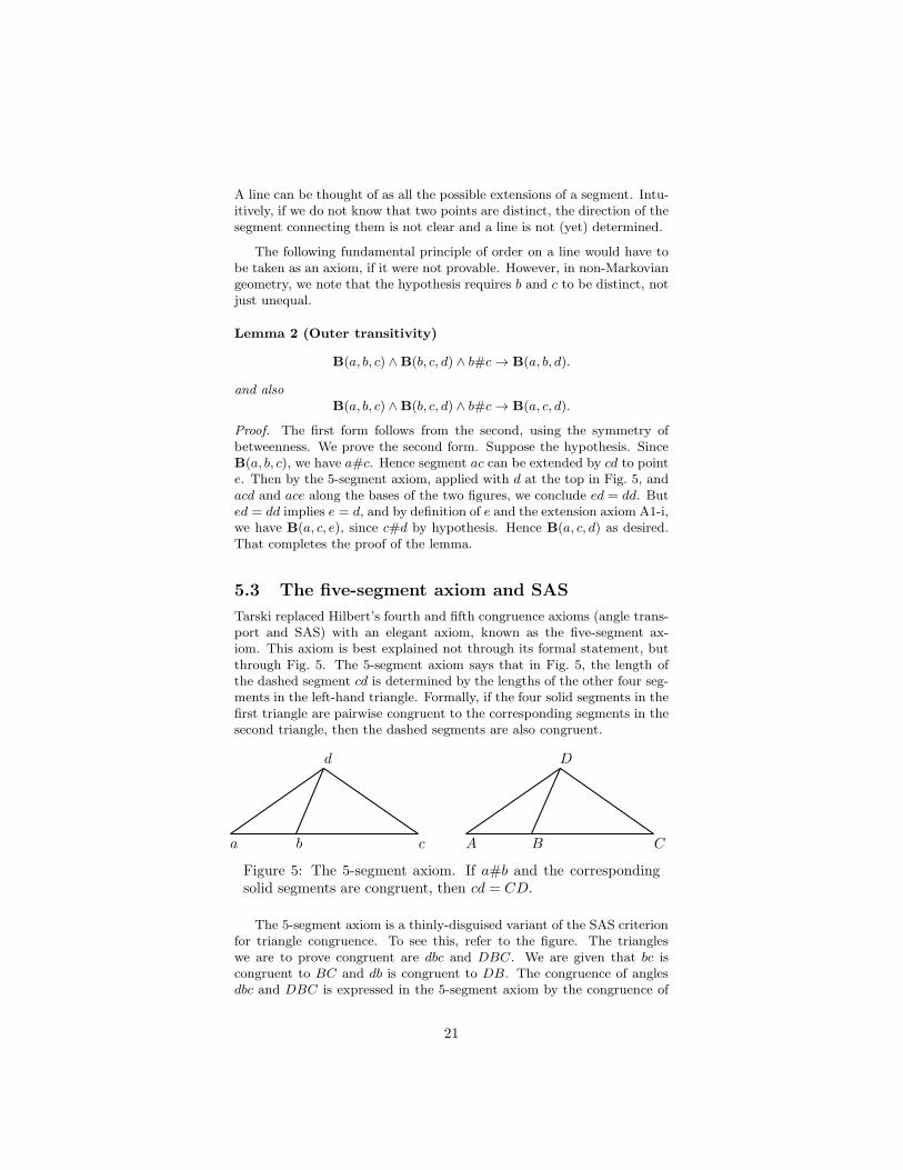
Proof. The first form follows from the second, using the symmetry ofbetweenness. We prove the second form. Suppose the hypothesis. SinceB(a, b, c), we have a#c. Hence segment ac can be extended by cd to pointe. Then by the 5-segment axiom, applied with d at the top in Fig. 5, andacd and ace along the bases of the two figures, we conclude ed = dd. Buted = dd implies e = d, and by definition of e and the extension axiom A1-i,we have B(a, c, e), since c#d by hypothesis. Hence B(a, c, d) as desired.That completes the proof of the lemma.

5.3 The five-segment axiom and SAS

Tarski replaced Hilbert’s fourth and fifth congruence axioms (angle trans-port and SAS) with an elegant axiom, known as the five-segment ax-iom. This axiom is best explained not through its formal statement, butthrough Fig. 5. The 5-segment axiom says that in Fig. 5, the length ofthe dashed segment cd is determined by the lengths of the other four seg-ments in the left-hand triangle. Formally, if the four solid segments in thefirst triangle are pairwise congruent to the corresponding segments in thesecond triangle, then the dashed segments are also congruent.

d

a b c

D

A B C

Figure 5: The 5-segment axiom. If a#b and the correspondingsolid segments are congruent, then cd = CD.

The 5-segment axiom is a thinly-disguised variant of the SAS criterionfor triangle congruence. To see this, refer to the figure. The triangleswe are to prove congruent are dbc and DBC. We are given that bc iscongruent to BC and db is congruent to DB. The congruence of anglesdbc and DBC is expressed in the 5-segment axiom by the congruence of

21

triangles abd and ABD, whose sides are pairwise equal. The conclusion,that cd is congruent to CD, gives the congruence of triangles dbc andDBC. In Chapter 11 of [26], one can find a formal proof of the SAScriterion from the 5-segment axiom. It is easily adapted to prove the SAScriterion in non-Markovian geometry (which in non-Markovian geometryrequires that the angle in question be positive).

The formal statement of the axiom uses non-strict betweenness anddoes not specify that d is not collinear with ab, though it does requirea 6= b. Allowing d to be collinear with ab permits the use of this axiom toderive properties of betweenness, and it is not only constructively valid,but very useful.

The question arises whether we ought to strengthen the hypothesisa 6= b to a#b, or even perhaps require B(a, b, c) (which would imply a#b,but also b#c). The latter would weaken the axiom.5 The former seemsphilosophically prudent, since without it, perhaps the direction of the lineab is uncertain. We therefore require a#b in this axiom.6

This axiom enables one to replace reasoning about angles with reason-ing about congruence of segments.7 We would like to emphasize that the5-segment axiom is often just as easy to use as SAS. Here is an illustrativeexample:

Lemma 3 Vertical angles are congruent.

Proof. Let angles abc and dbe be vertical angles; soB(a, b, e) andB(c, b, d).We may suppose without loss of generality that bd = bc = ab = be. Wemust show ac = de. Consider the two configurations abec and dbce. Thehypotheses of the 5-segment axiom are fulfilled, because ab = db, be = bc,ec = ce, and bc = be. Then by the 5-segment axiom, ac = de as desired.That completes the proof. The reader is urged to compare this proof toEuclid’s proof.

5.4 Lines, rays, triangles, and right angles

The segment extension axiom allows us to create a new point on theline containing a and b only when a and b are distinct points. WithoutMarkov’s principle, we have to distinguish between pairs of unequal points,and pairs of distinct points. In some sense only distinct points determinea segment, because only then does the segment extension axiom apply.Although Tarski’s language speaks only about points, the import of theaxiom is that we are allowed to construct the line containing a and b only

5The theorem “all null segments are equal” would not be provable; but adding it back asa new axiom would fix that. However, there seems no point in doing that.

6The unmodified 5-segment axiom holds in our Kripke model where Markov’s principlefails, so we are not mathematically compelled to modify it.

7The history of this axiom is as follows. The key idea (replacing reasoning about angles byreasoning about congruence of segments) was introduced (in 1904) by J. Mollerup [24]. Hissystem has an axiom closely related to the 5-segment axiom, and easily proved equivalent.Tarski’s version, however, is slightly simpler in formulation. Mollerup (without comment)gives a reference to Veronese [33]. Veronese does have a theorem (on page 241) with the samediagram as the 5-segment axiom, and closely related, but he does not suggest an axiom relatedto this diagram.

22

when a#b. Instead of “two unequal points determine a line”, we have“two distinct points determine a line”.

The relation of collinearity is defined by

L(a, b, c) ↔ ¬¬ (B(c, a, b) ∨ c = a ∨B(a, c, b) ∨ c = b ∨B(a, b, c)).

Pushing one negation sign inwards, L(a, b, c) can be expressed in a neg-ative form. Similarly, the notion that x is on the ray from b through ccan be expressed by L(b, c, x) ∧ ¬B(x, b, c). We write this as Ray(b, c, x).The ray itself is not treated as a mathematical object; only the relationbetween three points is formalized. Nevertheless we speak of x lying onRay(b, c), which is the same as saying Ray(b, c, x).

Lemma 4 Let a and b be distinct points. Let c and d be any points. Thenwe can lay segment cd off on Ray(a, b), in the sense that there exists apoint x with Ray(a, b, x) and ax = cd. Moreover, point x is unique.

Proof. Since a#b, segment ba can be extended to point e with ae = aband B(e, a, b). (We say e is the reflection of b in a.) Then segment eacan be extended by cd to point x. Then ax = cd and T(e, a, x), by thesegment extension axiom. But that is the meaning of Ray(a, b, x), so thefirst claim of the lemma is proved. It remains to prove the uniqueness of x.Suppose y is another point on Ray(a, b) with ay = cd. By the definitionof Ray(a, b, x), that means for some point e (the reflection of b in a) wehave T(e, a, x)∧T(e, a, y)∧ ax = ay. Now apply the 5-segment axiom tothe following two configurations in the form of Fig. 5: the first has eax onthe base and y on the top, the second has eay on the base and also has yon the top. The hypotheses are fulfilled because ax = ay. The conclusionis yx = yy. By Axiom A3, x = y. That completes the proof.

Definition 1 Angle abc is a right angle if a, b, and c are distinct points,and if d = ext(a, b, a, b) (so d is the reflection of a in b), then trianglesabc and dbc are congruent triangles.8

It can be proved that this notion respects the congruence relation onangles. Euclid’s Postulate 4, that all right angles are congruent, is atheorem in Tarski’s geometry.9 It can be proved (and without Markov’sprinciple). We do not have space in this paper to give the proof, but wewill outline it. The details can be found in [26], Part I, Chapter 10.

Reflection in a point is an isometry. That is, if B is the midpointof AC and also of PQ, then AP = CQ. The relation “ABC is a rightangle” is preserved under reflection in a point. Reflection in a line isan isometry. And the key result (Satz 10.12 in [26]): Given right anglesABC and ABF with BC congruent to BF , then AC is congruent to AF .(Remember there is no dimension axiom, so picture the two angles indifferent planes.) Here is a sketch of the proof:

8We note that in [26], the predicate R(a, b, c) allows the case b = c, but our definition of“right angle” requires three distinct points.

9It is a much simpler theorem in Hilbert’s geometry, because Hilbert takes as an axiomthat an angle can be copied on a given side of a given line, and the copy is unique. Thesefacts require non-trivial proofs from the axioms of EG or Tarski.

23

Let M be the midpoint of CF (which exists without needing circlessince triangle BCF is isosceles). Let D be the reflection of F in B,so ABD is congruent to ABF . Here is the key: triangle ABD is thereflection of ABC in the line BM . Since reflection in a line is a isometry,those triangles are congruent, proving Satz 10.12. Now given two rightangles, using Euclid’s Prop. 23 we can copy one of them into the positionof the second angle in Satz 10.12, and applying Satz 10.12, the angles arecongruent.

Lemma 5 If abc is a right angle, then cba is a right angle.

Proof. The two angles obtained by reflecting abc first in ba and then in bcare vertical angles, hence congruent. In fact the proof of Lemma 3 worksdirectly, without needing to first prove that an angle congruent to a rightangle is a right angle.

5.5 Positive angles

Corresponding to the notion of “distinct points”, there is, intuitively, anotion of “positive angle”, which we write abc > 0 (it is not necessary towrite ∠abc > 0). We also write this as 0 < abc; both our abbreviationsfor a statement involving betweenness (given below). Saying abc > 0 isstronger than simply requiring that a, b, and c are not collinear (with aand c on the same side of b) in the same way that apartness is stronger thaninequality. It is our immediate aim to define this notion. We wish thisnotion to be defined in such a way that, after we prove that coordinatescan be geometrically defined, the angle between p = (x, y) and q = (b, 0)with vertex at (0, 0) is a positive angle if and only if y > 0.10 But thiscannot be the definition, as many theorems must be proved before we canconstruct coordinates. For example, midpoints and perpendiculars areneeded.

We must define “positive angle” at the outset, because (as we shall seein the next section) we need to restrict the hypotheses of Pasch’s axiomby requiring an angle to be positive. Our first use of Pasch’s axiom will beto repair Euclid’s constructions in Propositions I.10 to I.10, culminatingin the theorem that every segment ab with a#b has a midpoint. In thatproof, we need to apply Pasch’s axiom in situations where the vertex angleis 30◦, 60◦, and 120◦. Therefore, the definition of “positive angle” mustimmediately imply that those angles are positive. More generally, we needto know that the angles of a right triangle are positive. (Remember that“triangle” implies the vertices are distinct.)

The following conversations, following the pattern of “light bulb” jokes,illustrate the basic concepts of non-Markovian geometry:

How many points does it take to determine a line? Three, twoto lay a straightedge on and one to check that the other two aredistinct.

10Here y > 0 refers to order on a line, defined axiomatically by betweenness, namelyB(−1, 0, y), where −1 and 0 are two specified points on a specified line.

24

How many points does it take to determine a positive angle?Six, three to determine the vertex and sides, one for each sideto check the other two are distinct, and the sixth to check thatthe sides do not coincide.

Definition 2 (i) abc is an apex angle if there are distinct points u, v onRay(b, a) and Ray(b, c) respectively such that bu = bv and b#u.

(ii) abc is an angle of a right triangle if bac or bca is a right angle,or more generally, if angle abc is congruent to an angle ABC such thatBAC or BCA is a right angle. “Right angle” is defined in Definition 1).

(iii) abc > 0 (“abc is a positive angle”) if abc is an apex angle, or aright angle, or an angle of a right triangle.

We will later prove that every positive angle is an apex angle, but thatcan be done only after developing some geometry, using the definitionabove. In other words, if we were to take “apex angle” as the definitionof “positive angle”, we could not prove that an angle of a right triangle ispositive, because to do so we need some intermediate results that cannotbe justified until we know that an angle of a right triangle is positive.Specifically, we will see below that a correct formulation of Pasch’s axiomfor non-Markovian geometry requires certain angles to be positive, and toprove that angles of a right triangle are apex angles, we need such anglesto be positive.

The formula abc > 0, written out in primitive notation, is existential,since not only is there an explicit ∃ and an explicit disjunction, but alsodistinctness involves an existential quantifier. This is good, since we in-tend it to express the existence of a positive lower bound on the angleabc.

We also need to express abc < π, i.e., angle abc is positively differentfrom a “straight angle.” We just need to say that the supplement of abcis a positive angle.

Definition 3 Angle abc has a positive supplement, or abc < π, is definedby

abc < π ↔ ∃d (B(a, b, d) ∧ dbc > 0).

We emphasize that the notation abc > 0 does not imply the assignmentof a measure of any kind to angles. It is just a statement that a pointcan be found to witness, using the betweenness relation, that the angleis not zero. To express that angle abc is both positive and has a positivesupplement, we abbreviate the conjunction of the two statements 0 < abcand abc < π as 0 < abc < π.

We can define certain specific angles as follows:

abc = 60◦ ↔ ab = bc ∧ ab = ac ∧#(a, b, c)

abc = 120◦ ↔ ∃d (B(a, b, d) ∧ ab = bd ∧ bc = bd ∧ cd = bc ∧#(a, b, c))

abc = 30◦ ↔ ∃d (B(a, d, b) ∧ ad = cd ∧ ad = db ∧#(a, b, c))

abc = 150◦ ↔ ∃d (B(a, b, d) ∧ cad = 30◦)

25

We would like to prove that each of these four angles is a positiveangle. That is neither obvious nor easy. In fact, to do so it is necessary tohave a strong lower dimension axiom. That issue will be discussed below;but the lower dimension axiom that we use guarantees the existence ofan equilateral triangle whose sides have midpoints, whose altitudes havedistinct endpoints, and whose medians meet in a central point. Thatconfiguration directly implies that 60◦ is an apex angle (hence positive),and 30◦ is an angle of a right triangle.

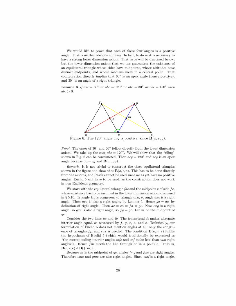
Lemma 6 If abc = 60◦ or abc = 120◦ or abc = 30◦ or abc = 150◦ thenabc > 0.

ba

bc

be

bf b g

b mb x

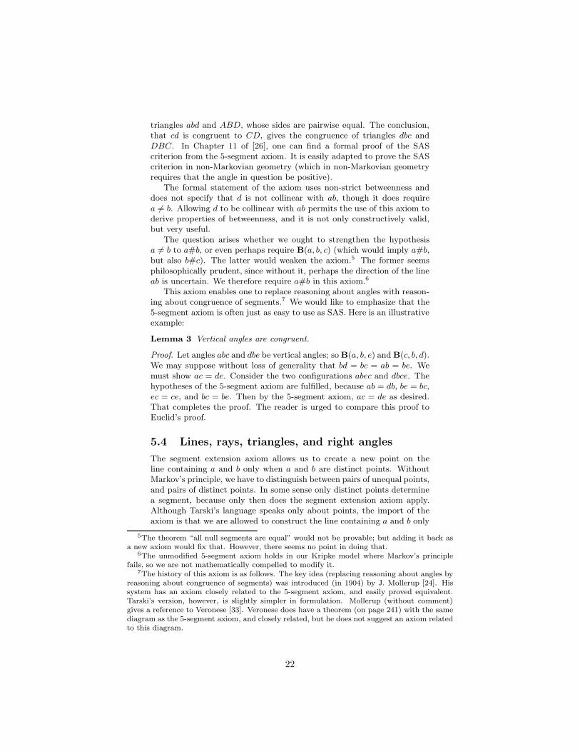
Figure 6: The 120◦ angle acg is positive, since B(a, x, g).

Proof. The cases of 30◦ and 60◦ follow directly from the lower dimensionaxiom. We take up the case abc = 120◦. We will show that the “tiling”shown in Fig. 6 can be constructed. Then acg = 120◦ and acg is an apexangle because ac = cg and B(a, x, g).

Remark. It is not trivial to construct the three equilateral trianglesshown in the figure and show that B(a, c, e). This has to be done directlyfrom the axioms, and Pasch cannot be used since we as yet have no positiveangles. Euclid 5 will have to be used, as the construction does not workin non-Euclidean geometry.

We start with the equilateral triangle fac and the midpoint x of side fc,whose existence has to be assumed in the lower dimension axiom discussedin § 5.10. Triangle fxa is congruent to triangle cxa, so angle axc is a rightangle. Then cxa is also a right angle, by Lemma 5. Hence gc = ac, bydefinition of right angle. Then ac = ca = fa = gc. Now cxg is a rightangle, so gxc is also a right angle, so fg = gc. Let m be the midpoint ofgc.

Consider the two lines ac and fg. The transversal fc makes alternateinterior angle equal, as witnessed by f , g, x, a, and c. Technically, ourformulation of Euclid 5 does not mention angles at all; only the congru-ence of triangles fgx and cax is needed. The condition B(g,m, c) fulfillsthe hypotheses of Euclid 5 (which would traditionally be expressed as“the corresponding interior angles mfc and ecf make less than two rightangles”). Hence fm meets the line through ac in a point e. That is,B(a, c, e) ∧B(f,m, e).

Because m is the midpoint of gc, angles fmg and fmc are right angles.Therefore cme and gme are also right angles. Since cmf is a right angle,

26

ce = fc = gc. Since emc is a right angle, ge = ce and triangle gce isequilateral. Then angle acg is, by definition, a 120◦ angle. But a#qbecause B(a, x, q). That completes the case of a 120◦ angle. fmc is aright angle, and mf = me, also fc = ce.

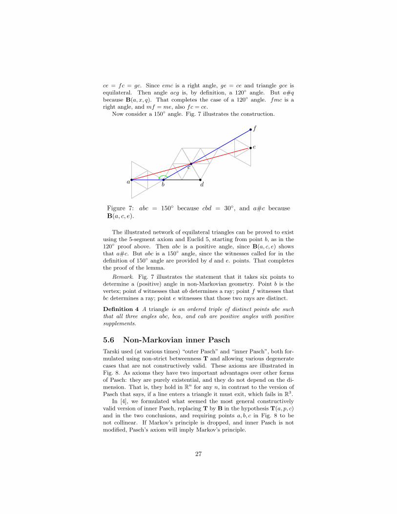
Now consider a 150◦ angle. Fig. 7 illustrates the construction.

b

bb

a

bc

b e

b

d

b f

Figure 7: abc = 150◦ because cbd = 30◦, and a#c becauseB(a, c, e).

The illustrated network of equilateral triangles can be proved to existusing the 5-segment axiom and Euclid 5, starting from point b, as in the120◦ proof above. Then abc is a positive angle, since B(a, c, e) showsthat a#c. But abc is a 150◦ angle, since the witnesses called for in thedefinition of 150◦ angle are provided by d and e. points. That completesthe proof of the lemma.

Remark. Fig. 7 illustrates the statement that it takes six points todetermine a (positive) angle in non-Markovian geometry. Point b is thevertex; point d witnesses that ab determines a ray; point f witnesses thatbc determines a ray; point e witnesses that those two rays are distinct.

Definition 4 A triangle is an ordered triple of distinct points abc suchthat all three angles abc, bca, and cab are positive angles with positivesupplements.

5.6 Non-Markovian inner Pasch

Tarski used (at various times) “outer Pasch” and “inner Pasch”, both for-mulated using non-strict betweenness T and allowing various degeneratecases that are not constructively valid. These axioms are illustrated inFig. 8. As axioms they have two important advantages over other formsof Pasch: they are purely existential, and they do not depend on the di-mension. That is, they hold in R

n for any n, in contrast to the version ofPasch that says, if a line enters a triangle it must exit, which fails in R

3.In [4], we formulated what seemed the most general constructively

valid version of inner Pasch, replacing T by B in the hypothesis T(a, p, c)and in the two conclusions, and requiring points a, b, c in Fig. 8 to benot collinear. If Markov’s principle is dropped, and inner Pasch is notmodified, Pasch’s axiom will imply Markov’s principle.

27

b

a xb q

bc

b b

bp

b

ab

qx

bb

b c

b

p

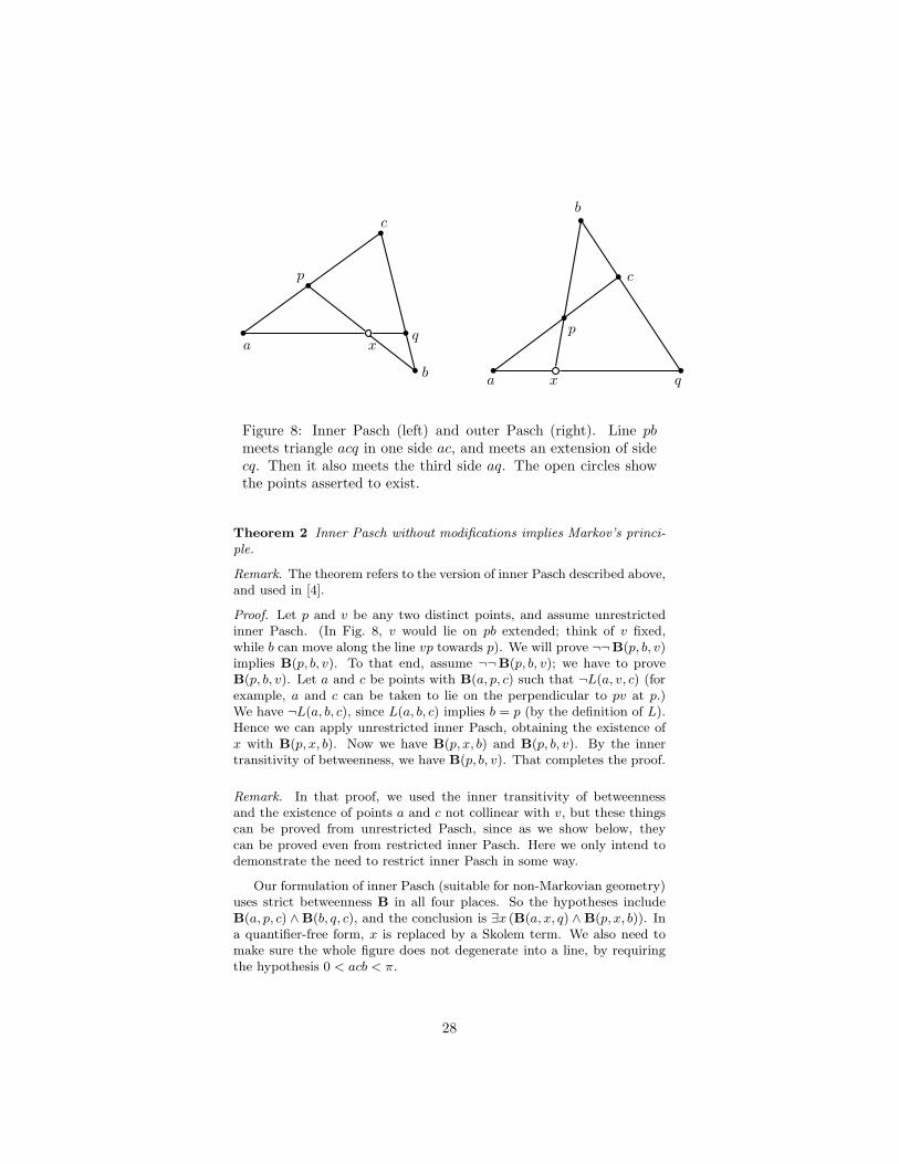
Figure 8: Inner Pasch (left) and outer Pasch (right). Line pb

meets triangle acq in one side ac, and meets an extension of sidecq. Then it also meets the third side aq. The open circles showthe points asserted to exist.

Theorem 2 Inner Pasch without modifications implies Markov’s princi-ple.

Remark. The theorem refers to the version of inner Pasch described above,and used in [4].

Proof. Let p and v be any two distinct points, and assume unrestrictedinner Pasch. (In Fig. 8, v would lie on pb extended; think of v fixed,while b can move along the line vp towards p). We will prove ¬¬B(p, b, v)implies B(p, b, v). To that end, assume ¬¬B(p, b, v); we have to proveB(p, b, v). Let a and c be points with B(a, p, c) such that ¬L(a, v, c) (forexample, a and c can be taken to lie on the perpendicular to pv at p.)We have ¬L(a, b, c), since L(a, b, c) implies b = p (by the definition of L).Hence we can apply unrestricted inner Pasch, obtaining the existence ofx with B(p, x, b). Now we have B(p, x, b) and B(p, b, v). By the innertransitivity of betweenness, we have B(p, b, v). That completes the proof.

Remark. In that proof, we used the inner transitivity of betweennessand the existence of points a and c not collinear with v, but these thingscan be proved from unrestricted Pasch, since as we show below, theycan be proved even from restricted inner Pasch. Here we only intend todemonstrate the need to restrict inner Pasch in some way.

Our formulation of inner Pasch (suitable for non-Markovian geometry)uses strict betweenness B in all four places. So the hypotheses includeB(a, p, c) ∧B(b, q, c), and the conclusion is ∃x (B(a, x, q) ∧B(p, x, b)). Ina quantifier-free form, x is replaced by a Skolem term. We also need tomake sure the whole figure does not degenerate into a line, by requiringthe hypothesis 0 < acb < π.

28

For comparison: Tarski used T instead of B, and did not care if thefigure degenerated. For constructive geometry, that is wrong, since it leadsto discontinuous dependence of x on the parameters. In [4], the hypothesisT(b, q, c) was retained but B was used for the other hypothesis and thetwo conclusions. That is, the degenerate cases q = c and q = b are stillallowed. This is constructively sensible as the lines aq and pb still aretransverse, so have a unique intersection point, constructible with a ruler.To avoid discontinuity, we also required ¬L(a, b, c).

In non-Markovian geometry, the negatively-phrased non-collinearity isnot enough, as the lemma above shows. Instead we need 0 < acb < π.The hypothesis 0 < acb < π is expressed in the way defined in § 5.5. Thatis an existential statement, but it occurs only in the hypotheses of innerPasch, so inner Pasch is still equivalent to a quantifier-free axiom (whena Skolem term is used for x).

There are, however, other possible hypotheses that we might also use inconnection with inner Pasch; that is, other possible sufficient conditionsthan 0 < acb < π that should support the conclusion of inner Paschwithout implying Markov’s principle. One such hypothesis is 0 < qpa < π.(Or equivalently, 0 < pqb < π.) This may seem strange (after all line pqis not even drawn in the diagram for Pasch’s axiom), but it is the naturalcondition that we need when we use inner Pasch to prove Euclid’s exteriorangle theorem. We were not able to prove the exterior angle theoremunless we take the form of inner Pasch with this hypothesis as an axiom,as well as the more natural 0 < acb < π. Of course, after developing thetheory of perpendiculars, we can prove these conditions equivalent, butto get off the ground we need both versions of inner Pasch.

5.7 Non-Markovian outer Pasch

Please refer to Fig. 8. The hypotheses of unrestricted outer Pasch in [4]are B(a, p, c) and T(b, c, q), as well as ¬L(a, b, c). The conclusion is thatthere exists an x such that B(a, x, q) and B(b, p, x).

Outer Pasch, like inner Pasch, in its unrestricted form implies Markov’sprinciple. The argument is similar to the one given for inner Pasch; inthe second part of Fig. 8, we allow a to move towards q, as for innerPasch we allowed b to move towards p. Therefore, outer Pasch needs tohave its hypotheses strengthened. As for inner Pasch, we replace T by B,and replace the non-collinearity hypotheses by requiring an angle to bebetween 0 and π. But which angle?

The hypothesis we choose to formulate non-Markovian outer Pasch isthis:

0 < baq < π ∨ 0 < abq < π.

This choice is a pragmatic one: it enables the uses of outer Pasch that weneed (in particular for the crossbar theorem). Eventually, we will provethat if a, b, and c are three distinct points, and one of three angles formedis positive, so are the other two. After that, the various possible versionsof non-Markovian outer Pasch will be equivalent.

Our theory EG includes both non-Markovian inner Pasch and non-Markovian outer Pasch as axioms. Gupta proved ([11]; see also [26], Satz

29

9.3), that inner Pasch implies outer Pasch; but this is a long development,and although we did not find a use of Markov’s principle, we are notwilling to certify that none is necessary. As mentioned above, we are notaiming in this paper to find a minimal set of axioms for EG, but instead asensible set of axioms that provides a smooth non-Markovian constructivedevelopment of Euclid. Therefore we include both forms of Pasch.

5.8 Line–circle and circle–circle continuity

We say that point p is inside the circle with center a passing through cprovided p lies on a diameter of the circle.11 The line–circle continuityaxiom says that if p is inside the circle with center a passing through c,then there exist two points x and y on the circle with B(x, p, y). Thisaxiom is true in R

n for any n, i.e., not just in plane geometry. Withoutany dimension axiom, “circles” become spheres (in R3) or hyperspheres.

We also need a non-strict version of line–circle continuity in which Bis replaced by non-strict betweenness T. Classically, the two are easilyproved equivalent, but the case distinction whether p is strictly inside oron the circle is not legitimate intuitionistically. Applied to Descartes’sgeometric construction of square roots, the non-strict version implies thatnon-negative segments have square roots, and the strict version impliesthat positive segments have positive square roots. We therefore need bothversions of line–circle continuity to establish the existence of coordinatesand define arithmetic.

The circle–circle continuity axiom says that if C and K are circles withdistinct centers, and C has a point non-strictly inside K, and a point non-strictly outside circle K, then there is a point lying on both C andK. Thisimmediately implies the corresponding strict version, but not conversely,so we take the non-strict version as our axiom.12

A stronger version of circle–circle continuity has the additional hy-pothesis that p is any point not lying on the line L containing the centersof C and K, and the additional conclusion that C and K have an inter-section point on the opposite side of L from p; that is, there are pointse and x with e on both C and K and x on L and B(e, x, p). We do notassume this stronger version of circle–circle continuity as an axiom.13

5.9 Segment-circle continuity

The segment-circle continuity principle says that if p is a point inside acircle, and q is a point outside, then there is a point on the circle be-

11It will not do to say p is equal to the center or lies on a radius, since we may not knowwhich alternative holds.

12We avoided “degenerate cases” of Pasch’s axiom, in which a two-dimensional picturedegenerates to one dimension. Using T in the circle–circle axiom is not a degenerate case inthis sense; when the circles are tangent, the picture is still two-dimensional.

13This means that Euclid’s proof of I.4 (angle bisection) is not directly formalizable in EG,and his proof of the existence of a midpoint is consequently also not directly formalizable.Instead, we construct midpoints using Gupta’s theorem about the existence of a midpoint ofan isosceles triangle, combined with Euclid’s construction of an equilateral triangle on a givensegment. Once midpoints are in hand, perpendiculars can be constructed, and the strongerversion of circle–circle continuity can be proved.

30

tween p and q. This principle has been suggested as an axiom by manyauthors, including Tarski (see [27]). But a detailed study shows that it isinadequate; an irremovable circularity arises in formalizing Euclid with-out a dimension axiom. If we try to construct dropped perpendiculars(Euclid I.12) using segment-circle continuity, to check the hypotheses weneed the triangle inequality (I.20). But I.19 is needed for I.20, and I.7 forI.19. In Prop. I.7, the two triangles that are supposed to coincide maylie in different planes; that possibility has to be removed by an additionalhypothesis. Even with its statement thus corrected, I.7 is more difficultto prove than Euclid thought, since he took for granted the fact that anangle cannot be less than itself, but that principle is actually the essentialcontent of I.7. Ever since Hilbert [15], angle inequality has been regardedas a defined concept, and proving I.7 then requires dropped perpendic-ulars (I.12). But this is circular. The conclusion is that segment-circlecontinuity is not a suitable axiom to use in formalizing Euclid.14

5.10 Dimension axioms

When considering plane geometry, one needs a lower dimension axiomproviding for the existence of three non-collinear points. Non-collinearitywill not be enough in non-Markovian geometry; we need to ensure thatthere exist three points forming a positive angle with a positive supple-ment. In other words, we need three distinct points α, β, and γ such that0 < αβγ < π.15

We take as an axiom that there are three points, given by constantsα1, α2, α3, that form an equilateral triangle. Then we add a furtheraxiom, introducing three more constants for the midpoints of the threesides, and one final constant for the common intersection point of twoof the medians. Thus the three vertices are all distinct, and two of themedians have distinct endpoints. See Fig. 9. The formal expression ofthis axiom is given in the next section, where all the axioms are listed forreference.

The upper dimension axiom for plane geometry says that if a and b aredistinct, and three points are each equidistant from a and b, then thosethree points are collinear. If we do not use any upper dimension axiom, orwe replace 3 by some larger integer, then as we have already noted, innerand outer Pasch still make sense, and circle–circle continuity becomes

14line–circle continuity does not suffer from this problem, as the triangle inequality is notrequired to drop perpendiculars. Of course, as Gupta showed, one can construct droppedperpendiculars without mentioning circles at all, so there is no formal result that one continuityaxiom is better for I.7 than another, as none at all is actually needed. We merely say thatEuclid’s proof can be repaired with line–circle, but not with segment-circle.

15If we do not specify this in an axiom, nothing allows to prove any betweenness state-ment, as the first deduction of a betweenness statement cannot come from the betweennessaxioms (which have betweenness hypotheses), nor from Pasch (which has betweenness in thehypothesis about a positive angle), nor from the extension axiom, which requires betweennessin the hypothesis about distinct points, nor from circle–circle or line–circle continuity, wherethe hypotheses about “inside” are expressed using betweenness. Nothing would prevent theplane from collapsing, with all points not not equal to each other. Hence, it is reasonable tocall this a “lower dimension axiom”.

31

bβ

bγ

bα

b c2

c4

bc1b

bc3

Figure 9: The lower dimension axiom

sphere–sphere continuity. The notions “same side” and “opposite side” ofa line still make sense if properly defined. See [4] for the definitions.

5.11 List of axioms for reference

In this section, we give the complete list of axioms of EG. First, we specifythe language. It is first-order predicate calculus with equality. Thereis a 3-ary relation symbol B and a 4-ary symbol E. E is the officialversion of the 4-ary relation that we write informally as ab = cd; first-orderpredicate calculus as found in textbooks does not permit that syntax, soab = cd must remain as an informal abbreviation for the more formalsyntax E(a, b, c, d).

A number of other informal abbreviations are used in stating the ax-ioms. The actual axioms are the result of replacing these abbreviationsby the right-hand side of their definitions (recursively), so the axioms in-volve only equality, B, and E. The following is a complete list of theseabbreviations. Since each right-hand side involves only definitions earlierin the list, the recursive replacement mentioned does terminate. That is,there is no circularity in this list of definitions.

a#b := ∃c (B(c, a, b) ∨B(a, c, b) ∨B(a, b, c))

ab = cd := E(a, b, c, d)

R(a, b, c) := ∃d (B(a, b, d) ∧ ab = bd ∧ ac = dc ∧ a#b ∧ c#b ∧ a#c)Ray(a, b, x) := ∃d (B(d, a, b) ∧B(b, a, x))

apex(a, b, c) := ∃u, v (Ray(b, a, u) ∧ Ray(b, c, v) ∧ bu = bv ∧ u#v)∠abc = ∠ABC := ∃U, V, u, v (Ray(b, a, u) ∧ Ray(b, c, v)

∧Ray(B,A,U) ∧Ray(B,C, V ) ∧ uv = UV )

0 < abc := apex(a, b, c) ∨ R(a, b, c) ∨∃A,B,C (∠abc = ∠ABC ∧R(B,A,C) ∨R(A,C,B))

abc < π := ∃d (B(d, b, a) ∧ 0 < dbc)

0 < abc < π := 0 < abc ∧ abc < π

T(a, b, c) := ¬(a 6= b ∧ ¬B(a, b, c) ∧ b 6= c)

32

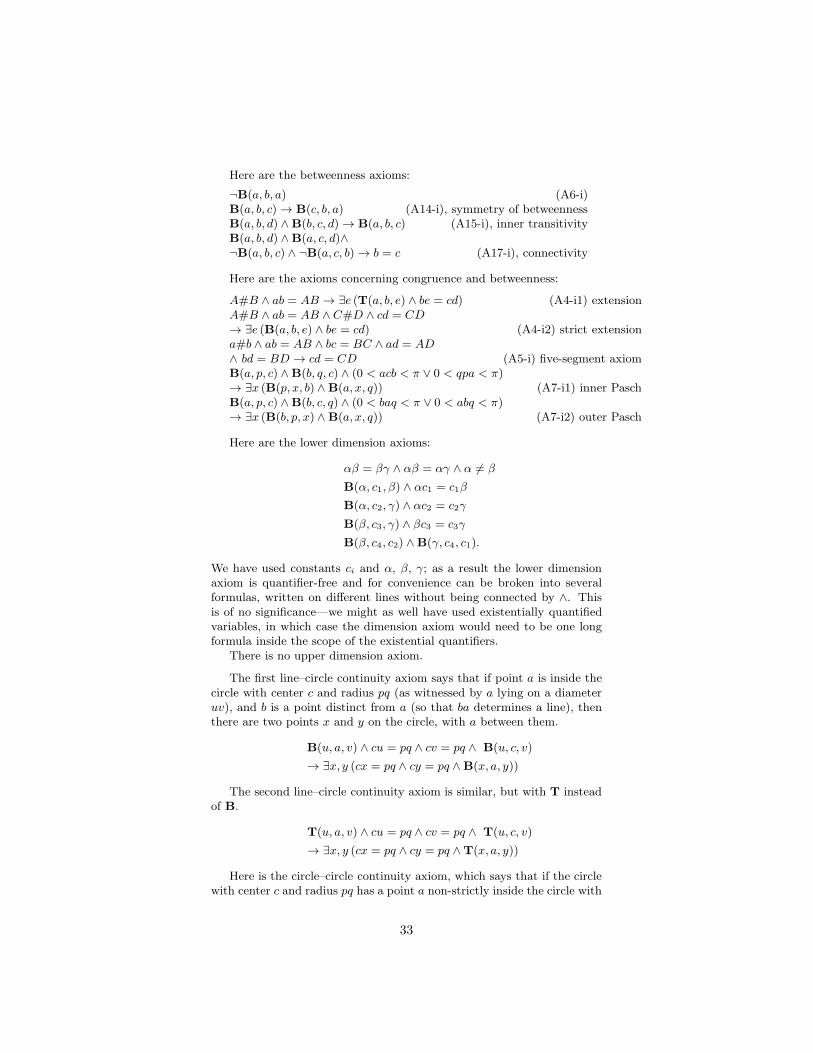
Here are the betweenness axioms:

¬B(a, b, a) (A6-i)B(a, b, c) → B(c, b, a) (A14-i), symmetry of betweennessB(a, b, d) ∧B(b, c, d) → B(a, b, c) (A15-i), inner transitivityB(a, b, d) ∧B(a, c, d)∧¬B(a, b, c) ∧ ¬B(a, c, b) → b = c (A17-i), connectivity

Here are the axioms concerning congruence and betweenness:

A#B ∧ ab = AB → ∃e (T(a, b, e) ∧ be = cd) (A4-i1) extensionA#B ∧ ab = AB ∧ C#D ∧ cd = CD→ ∃e (B(a, b, e) ∧ be = cd) (A4-i2) strict extensiona#b ∧ ab = AB ∧ bc = BC ∧ ad = AD∧ bd = BD → cd = CD (A5-i) five-segment axiomB(a, p, c) ∧B(b, q, c) ∧ (0 < acb < π ∨ 0 < qpa < π)→ ∃x (B(p, x, b) ∧B(a, x, q)) (A7-i1) inner PaschB(a, p, c) ∧B(b, c, q) ∧ (0 < baq < π ∨ 0 < abq < π)→ ∃x (B(b, p, x) ∧B(a, x, q)) (A7-i2) outer Pasch

Here are the lower dimension axioms:

αβ = βγ ∧ αβ = αγ ∧ α 6= β

B(α, c1, β) ∧ αc1 = c1β

B(α, c2, γ) ∧ αc2 = c2γ

B(β, c3, γ) ∧ βc3 = c3γ

B(β, c4, c2) ∧B(γ, c4, c1).

We have used constants ci and α, β, γ; as a result the lower dimensionaxiom is quantifier-free and for convenience can be broken into severalformulas, written on different lines without being connected by ∧. Thisis of no significance—we might as well have used existentially quantifiedvariables, in which case the dimension axiom would need to be one longformula inside the scope of the existential quantifiers.

There is no upper dimension axiom.

The first line–circle continuity axiom says that if point a is inside thecircle with center c and radius pq (as witnessed by a lying on a diameteruv), and b is a point distinct from a (so that ba determines a line), thenthere are two points x and y on the circle, with a between them.

B(u, a, v) ∧ cu = pq ∧ cv = pq ∧ B(u, c, v)

→ ∃x, y (cx = pq ∧ cy = pq ∧B(x, a, y))

The second line–circle continuity axiom is similar, but with T insteadof B.

T(u, a, v) ∧ cu = pq ∧ cv = pq ∧ T(u, c, v)

→ ∃x, y (cx = pq ∧ cy = pq ∧T(x, a, y))

Here is the circle–circle continuity axiom, which says that if the circlewith center c and radius pq has a point a non-strictly inside the circle with

33

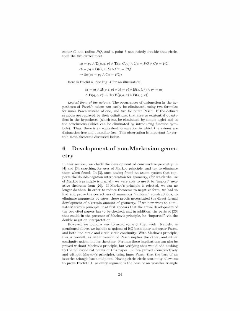
center C and radius PQ, and a point b non-strictly outside that circle,then the two circles meet.

ca = pq ∧T(u, a, v) ∧T(u,C, v) ∧ Cu = PQ ∧ Cv = PQ

cb = pq ∧B(C,w, b) ∧ Cw = PQ

→ ∃e (ce = pq ∧ Ce = PQ)

Here is Euclid 5. See Fig. 4 for an illustration.

pt = qt ∧B(p, t, q) ∧ st = rt ∧B(s, t, r) ∧ pr = qs

∧ B(q, a, r) → ∃e (B(p, a, e) ∧B(s, q, e))

Logical form of the axioms. The occurrences of disjunction in the hy-potheses of Pasch’s axiom can easily be eliminated, using two formulasfor inner Pasch instead of one, and two for outer Pasch. If the definedsymbols are replaced by their definitions, that creates existential quanti-fiers in the hypotheses (which can be eliminated by simple logic) and inthe conclusions (which can be eliminated by introducing function sym-bols). Thus, there is an equivalent formulation in which the axioms aredisjunction-free and quantifier free. This observation is important for cer-tain meta-theorems discussed below.

6 Development of non-Markovian geom-

etry

In this section, we check the development of constructive geometry in[4] and [3], searching for uses of Markov principle, and try to eliminatethem when found. In [3], once having found an axiom system that sup-ports the double-negation interpretation for geometry, (for which the useof Markov’s principle is crucial), we were able to use it to “import” neg-ative theorems from [26]. If Markov’s principle is rejected, we can nolonger do that. In order to reduce theorems to negative form, we had tofind and prove the correctness of numerous “uniform” constructions, toeliminate arguments by cases; those proofs necessitated the direct formaldevelopment of a certain amount of geometry. If we now want to elimi-nate Markov’s principle, it at first appears that the entire development ofthe two cited papers has to be checked, and in addition, the parts of [26]that could, in the presence of Markov’s principle, be “imported” via thedouble negation interpretation.

However, we found a way to avoid some of that work. Namely, asmentioned above, we include as axioms of EG both inner and outer Pasch,and both line–circle and circle–circle continuity. With Markov’s principle,this is overkill, as either version of Pasch implies the other, and eithercontinuity axiom implies the other. Perhaps these implications can also beproved without Markov’s principle, but verifying that would add nothingto the philosophical points of this paper. Gupta proved (constructivelyand without Markov’s principle), using inner Pasch, that the base of anisosceles triangle has a midpoint. Having circle–circle continuity allows usto prove Euclid I.1, so every segment is the base of an isosceles triangle

34

and hence has a midpoint. From there we can proceed to perpendicularsand thence to the main body of [4], eliminating the need to check [26]. Inparticular, we need to check neither Gupta’s proof of outer Pasch nor hisconstruction of midpoints without using circles, both of which are longand difficult. Why then, do we need outer Pasch? Aside from its innateinterest, outer Pasch is the key tool to prove the plane separation theorem,Theorem 2.5 of [3].16

6.1 Midpoints

Euclid’s own midpoint construction (Prop. I.10) is to construct an isosce-les triangle on pq and then bisect the vertex angle. But Euclid’s proof isdefective; a correct proof has to rely on Pasch’s axiom. Gupta showed in1965 [11] how to construct midpoints without using circles. His proof iscomplicated, but we are allowed to use circles, so Gupta’s construction isirrelevant for this paper.

One of Gupta’s “simpler” theorems enables us to justify the secondpart of this Euclidean midpoint construction, and we present the mainconstruction of that lemma next, for the reader’s enjoyment (it is shortand beautiful), and because we need to check (in the next lemma) that itrelies only on a version of Pasch that is acceptable when Markov’s principleis rejected.

Theorem 3 (Gupta) Assuming Markov’s principle, the base of an isosce-les triangle always has a midpoint.

b

Cb

B

b E

b

D

bA

F

b

Cb

B

b E

b

D

bA

M

bF

Figure 10: To construct the midpoint M of AB, given C with AC

equal to BC, constructing first F and then M by inner Pasch.

Proof. See page 56 of [11]. We repeat the proof here, because below wewill adapt it to work without Markov’s principle. First we just repeat itas Gupta gave it. We are not claiming that this proof works in EG.

Let ABC be an isosceles triangle with AC equal to BC. It is desiredto find the midpoint M of AB. Let α and β be any two distinct points,

16Gupta’s proof of outer Pasch from inner Pasch does not use the parallel axiom. Thatraises the possibility that it might be easy to prove outer Pasch if we allow the use of theparallel axiom. But then, we have to ask which version of the parallel axiom. In [3], Theorem9.2, we show that Euclid 5 implies Tarski’s parallel axiom, but we used outer Pasch in theproof. It is not difficult to prove that Tarski’s parallel axiom plus inner Pasch implies outerPasch. But we do not have a short proof of outer Pasch from Euclid 5. We do have a shortproof of inner Pasch from outer Pasch and Euclid 5.

35

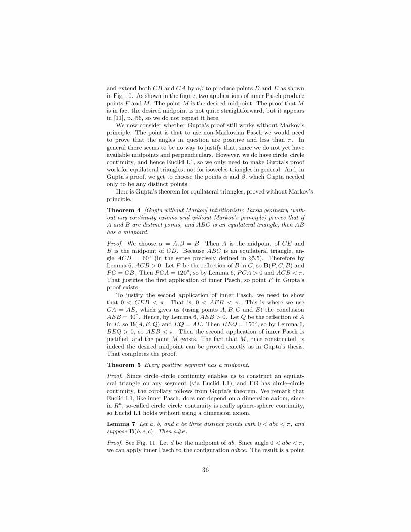
and extend both CB and CA by αβ to produce points D and E as shownin Fig. 10. As shown in the figure, two applications of inner Pasch producepoints F andM . The pointM is the desired midpoint. The proof thatMis in fact the desired midpoint is not quite straightforward, but it appearsin [11], p. 56, so we do not repeat it here.

We now consider whether Gupta’s proof still works without Markov’sprinciple. The point is that to use non-Markovian Pasch we would needto prove that the angles in question are positive and less than π. Ingeneral there seems to be no way to justify that, since we do not yet haveavailable midpoints and perpendiculars. However, we do have circle–circlecontinuity, and hence Euclid I.1, so we only need to make Gupta’s proofwork for equilateral triangles, not for isosceles triangles in general. And, inGupta’s proof, we get to choose the points α and β, which Gupta neededonly to be any distinct points.

Here is Gupta’s theorem for equilateral triangles, proved without Markov’sprinciple.

Theorem 4 [Gupta without Markov] Intuitionistic Tarski geometry (with-out any continuity axioms and without Markov’s principle) proves that ifA and B are distinct points, and ABC is an equilateral triangle, then ABhas a midpoint.

Proof. We choose α = A, β = B. Then A is the midpoint of CE andB is the midpoint of CD. Because ABC is an equilateral triangle, an-gle ACB = 60◦ (in the sense precisely defined in §5.5). Therefore byLemma 6, ACB > 0. Let P be the reflection of B in C, so B(P,C,B) andPC = CB. Then PCA = 120◦, so by Lemma 6, PCA > 0 and ACB < π.That justifies the first application of inner Pasch, so point F in Gupta’sproof exists.

To justify the second application of inner Pasch, we need to showthat 0 < CEB < π. That is, 0 < AEB < π. This is where we useCA = AE, which gives us (using points A,B,C and E) the conclusionAEB = 30◦. Hence, by Lemma 6, AEB > 0. Let Q be the reflection of Ain E, so B(A,E,Q) and EQ = AE. Then BEQ = 150◦, so by Lemma 6,BEQ > 0, so AEB < π. Then the second application of inner Pasch isjustified, and the point M exists. The fact that M , once constructed, isindeed the desired midpoint can be proved exactly as in Gupta’s thesis.That completes the proof.

Theorem 5 Every positive segment has a midpoint.

Proof. Since circle–circle continuity enables us to construct an equilat-eral triangle on any segment (via Euclid I.1), and EG has circle–circlecontinuity, the corollary follows from Gupta’s theorem. We remark thatEuclid I.1, like inner Pasch, does not depend on a dimension axiom, sincein Rn, so-called circle–circle continuity is really sphere-sphere continuity,so Euclid I.1 holds without using a dimension axiom.

Lemma 7 Let a, b, and c be three distinct points with 0 < abc < π, andsuppose B(b, e, c). Then a#e.

Proof. See Fig. 11. Let d be the midpoint of ab. Since angle 0 < abc < π,we can apply inner Pasch to the configuration adbce. The result is a point

36

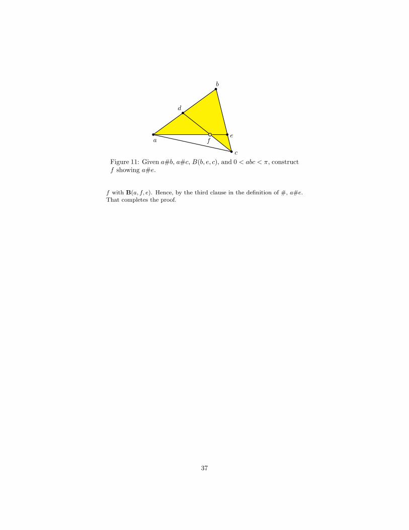
b

a f

b e

bb

b c

bd

Figure 11: Given a#b, a#c, B(b, e, c), and 0 < abc < π, constructf showing a#e.

f with B(a, f, e). Hence, by the third clause in the definition of #, a#e.That completes the proof.

37

6.2 Uniform perpendicular

In [3], we gave two different constructions of the uniform perpendicular(to a line L through a point p, without assuming that p is or is not online L). One construction assumes the parallel axiom, but not line–circlecontinuity. The other assumes line–circle continuity, but not the parallelaxiom. (It is an open problem to do it without assuming either of thetwo.) In this paper, we assume both those two hypotheses, so we candisregard the comparatively difficult construction that avoids line–circlecontinuity. The other construction is fairly straightforward: just draw a“large enough” circle C about point p (large enough that C meets L intwo points a and b with a#b), and then bisect segment ab to find the footf of the perpendicular, and then erect the perpendicular to L at f , usingthe construction of Euclid I.1 to construct an equilateral triangle over aband connect its vertex to f . The only tricky part of this construction is tofind the radius to use to draw C. Line L is given by two points, say u andv, with u#v. So segment uv can be extended; extend it by pu (which maybe null or not, we do not care) and again by pv. The resulting segment isat least uv longer than pu or pv, so it can serve as the radius of C.

6.3 Euclid does not need Markov

Does Markov’s principle, or the stability of congruence, actually play animportant role in Euclidean reasoning? We searched for a theorem inEuclid Books I-IV in which Markov’s principle is needed. There is an apriori constraint, which we consider first.

First, the double negation interpretation. For simplicity we considerthe version of EG based on Tarski’s language and axioms, with Skolemsymbols ext for the segment-extension axiom, ip for inner Pasch, and e5 forEuclid 5. As discussed at the end of §5.11, the axioms are then quantifier-free and can be put in the form A→ B, where A and B are conjunctions ofatomic formulas. Let φ− be the double-negation interpretation of φ. Sincedouble negation commutes with implication and conjunction, each axiomφ satisfies φ− ↔ ¬¬ φ. Each theorem ψ of Euclid is also of the form justdescribed. Hence, if the conclusion of ψ mentions only congruence andequality (and not betweenness), then we will have ψ− → ψ, in EG plus thestability of congruence. Therefore, any theorem of Euclid that actuallyrequires Markov’s principle must mention betweenness in its (formalized)conclusion.

We therefore examined the propositions of Euclid looking for theoremswhose conclusions involve collinearity, angle ordering, or segment ordering.This investigation is slightly complicated, because Euclid contains well-known errors, and because Euclid has never yet been formalized faithfully(i.e., in a theory that permits correcting Euclid’s proofs, while assumingnot too much more than Euclid did).17 Nevertheless, those errors can be

17There have certainly been many correct formal theories of geometry capable of provingversions of the propositions of Euclid. But that is not quite the same thing as formalizingEuclid. For example, to get the two circles in Proposition I.1 to intersect, clearly Euclid isimplicitly assuming some kind of circle–circle continuity. But Euclid has no dimension axiom,so circles are really “spheres”. Did Euclid intend to assume that two circles intersect on a

38

corrected, so the search for a possible use of Markov’s principle is possible,even in this rough terrain.

The first one is Euclid I.14, which says

If with any straight line, and at a point on it, two straight linesnot lying on the same side make the adjacent angles equal totwo right angles, the two straight lines will be in a straight linewith one another.

The collinearity statement in the conclusion is naturally expressed usingbetweenness. For a diagram, refer to your copy of Euclid. Our point aboutthis example is that stability of betweenness is not actually needed. Let E(in Euclid’s figure) lie on CB extended, with BE = BC. Let PB ⊥ BC;then CBP and PBE are right angles, so CBA and ABE are equal to tworight angles. Hence angles CBA and ABE together equal angles CBAand ABD. Hence angle ABE equals angle ABD. It follows that E andD lie on the same line CBE on the same side of B. (That follows inTarski’s system from the definition of equality of angles.) We do not needthe argument using Markov’s principle that Euclid gives in I.14.

6.4 The exterior angle theorem and its conse-

quences

The next potential example is I.16, the exterior angle theorem. Euclid’sproof constructs a crucial point F , but he left a gap in failing to provethat F lies in the interior of a certain angle.

The proof is also instructive, for those not yet completely familiar withTarski’s treatment of angles, in that it shows how to “unwind” a theoremabout angles, to see what it “really states” when angles are eliminated infavor of a points-only formulation.

Lemma 8 (Exterior angle theorem, Euclid I.16) Suppose B(B,C,D)and A#B and 0 < BAC < π. Then ACD > BAC.

Remark. The hypotheses are weaker than “ABC is a triangle”, whichby definition requires all three angles to be positive and have positivesupplements.

Proof. Euclid’s diagram is extended by Fig. 12. We show how to completeEuclid’s proof. To prove ACD > BAC, we must construct a point F inthe interior of ACD such that ACF = BAC. Euclid knew what angleordering means: he constructs F as shown in the figure. We can constructE (and hence F ) without Markov’s principle, since by Lemma 7, B#E,so segment BE can be extended as required. The lemma is applicable bythe hypothesis 0 < BAC < π.

given side of the line connecting their centers, or just that they intersect somewhere? If onlythe latter, then his proof that an angle could be bisected is wrong. If the former, then hewould not need to bisect an angle first, but could bisect a segment directly by constructingtwo equilateral triangles on opposite sides of the segment. Proposition 7 patently fails inthree-space, so perhaps Euclid did mean to have a dimension axiom. But eventually he workson the Platonic solids, so he needs to not have a dimension axiom.

39

bA

b

Cb

D

bE

b

F

H

b

B

Figure 12: Triangle ABC has exterior angle ACD. E is themidpoint of AC and also of BF . H exists by inner Pasch.

Euclid neglects to prove that F lies in the interior of ACD. To fill thisgap in Euclid, we need point H in the figure to exist. We wish to obtain Hfrom inner Pasch, applied to the five-point configuration shaded in Fig. 12.But to use inner Pasch in Markov-free geometry, we need an appropriateangle to be positive. It would suffice to show that 0 < FBC < π, butthere seems to be no way to do that until the theory of positive anglesis developed, which cannot precede the exterior angle theorem. However,our formulation of inner Pasch allows it to be applied if 0 < ECF < π.

Since E is the midpoint of both AC and BF , and vertical angles areequal (Lemma 3), triangles AEB and CEF are congruent, and trianglesAEF and CEB are congruent, by the SAS congruence theorem (EuclidI.2); that is, AF = CB. Then triangles ABC and CFA are also congruent;hence angle BAC is equal to angle FCA. Since 0 < BAC < π, we have0 < FCA < π. But angle FCA is equal to angle FCE, since B(C,E,A).Angle FCE is equal to angle ECF . Therefore 0 < ECF < π, justifyingthe desired application of inner Pasch. That completes the proof that Fis in the interior of angle ACD, which in turn completes the proof of theexterior angle theorem.

Remark. It is an open question whether the exterior angle theorem is stillprovable if inner Pasch is formulated with only the hypothesis 0 < acb < πinstead of the hypothesis 0 < acb < π ∨ 0 < pqb < π. We tried variousways of applying outer Pasch without success.

The immediate corollary (Euclid I.17) is that any two angles of atriangle, taken together, are less than two right angles. In particular,no triangle contains two right angles.

Lemma 9 In a right triangle, the hypotenuse is greater than either leg.

Proof. First prove Euclid I.18 and I.19. Then apply them as indicated inExercise 22, p. 198 of [10]. Alternately, see Satz 11.46 of [26]; the proofthere uses nothing but elementary betweenness and congruence, and theexistence of perpendiculars.

6.5 Crossbar theorem

The “crossbar theorem” proved in this section is an easy consequence ofouter Pasch, but I do not know how to derive it from inner Pasch (withoutMarkov’s principle).

40

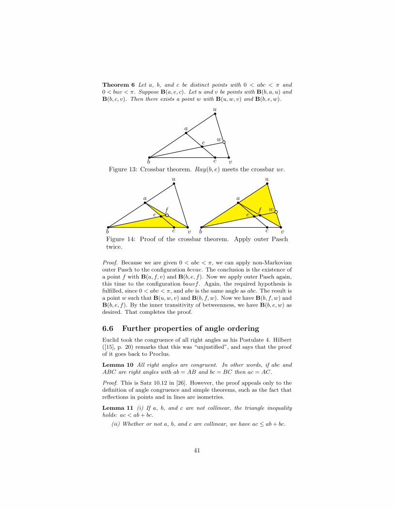
Theorem 6 Let a, b, and c be distinct points with 0 < abc < π and0 < buv < π. Suppose B(a, e, c). Let u and v be points with B(b, a, u) andB(b, c, v). Then there exists a point w with B(u,w, v) and B(b, e, w).

ba

bew

bu

bc

b

vb

b

Figure 13: Crossbar theorem. Ray(b, e) meets the crossbar uv.

ba

bef

bu

bc

b

vb

b

ba

be bf w

bu

bc

b

vb

b

Figure 14: Proof of the crossbar theorem. Apply outer Paschtwice.

Proof. Because we are given 0 < abc < π, we can apply non-Markovianouter Pasch to the configuration bcvae. The conclusion is the existence ofa point f with B(a, f, v) and B(b, e, f). Now we apply outer Pasch again,this time to the configuration bauvf . Again, the required hypothesis isfulfilled, since 0 < abv < π, and abv is the same angle as abc. The result isa point w such that B(u,w, v) and B(b, f, w). Now we have B(b, f, w) andB(b, e, f). By the inner transitivity of betweenness, we have B(b, e, w) asdesired. That completes the proof.

6.6 Further properties of angle ordering

Euclid took the congruence of all right angles as his Postulate 4. Hilbert([15], p. 20) remarks that this was “unjustified”, and says that the proofof it goes back to Proclus.

Lemma 10 All right angles are congruent. In other words, if abc andABC are right angles with ab = AB and bc = BC then ac = AC.

Proof. This is Satz 10.12 in [26]. However, the proof appeals only to thedefinition of angle congruence and simple theorems, such as the fact thatreflections in points and in lines are isometries.

Lemma 11 (i) If a, b, and c are not collinear, the triangle inequalityholds: ac < ab+ bc.

(ii) Whether or not a, b, and c are collinear, we have ac ≤ ab+ bc.

41

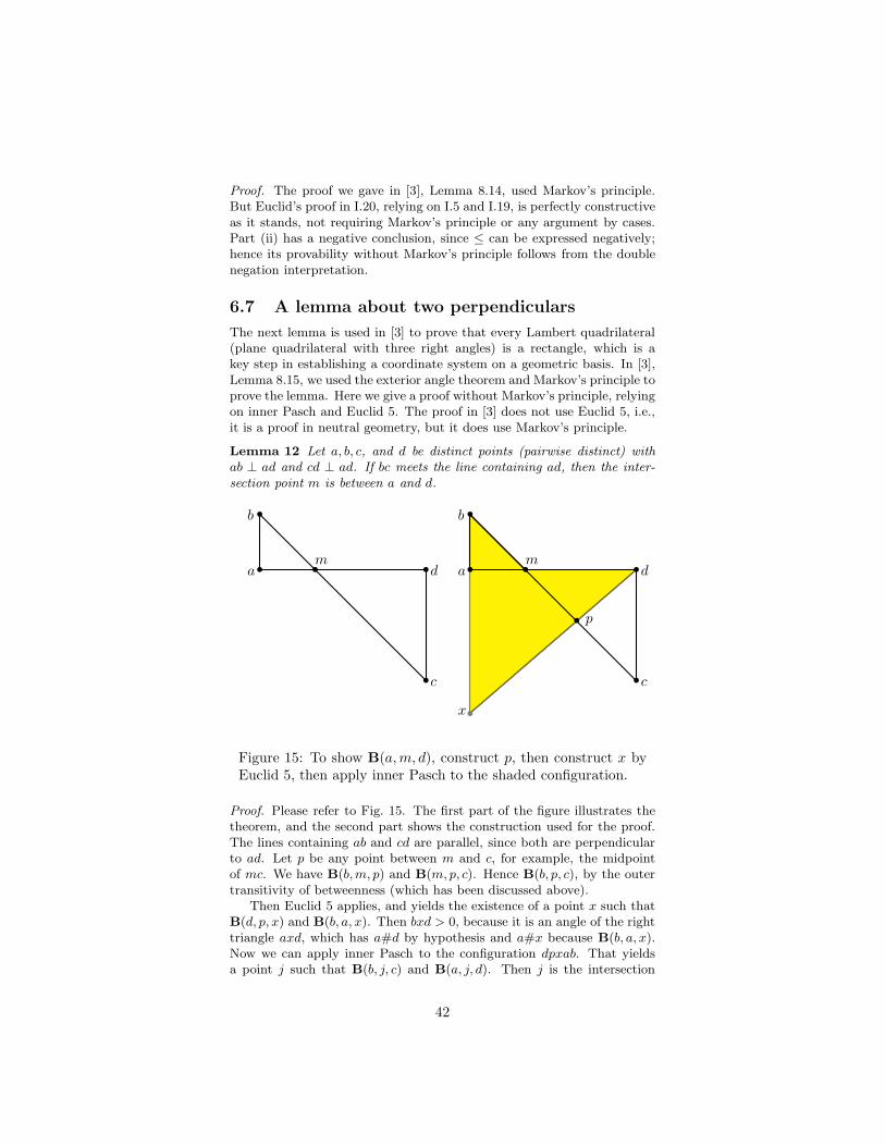
Proof. The proof we gave in [3], Lemma 8.14, used Markov’s principle.But Euclid’s proof in I.20, relying on I.5 and I.19, is perfectly constructiveas it stands, not requiring Markov’s principle or any argument by cases.Part (ii) has a negative conclusion, since ≤ can be expressed negatively;hence its provability without Markov’s principle follows from the doublenegation interpretation.

6.7 A lemma about two perpendiculars

The next lemma is used in [3] to prove that every Lambert quadrilateral(plane quadrilateral with three right angles) is a rectangle, which is akey step in establishing a coordinate system on a geometric basis. In [3],Lemma 8.15, we used the exterior angle theorem and Markov’s principle toprove the lemma. Here we give a proof without Markov’s principle, relyingon inner Pasch and Euclid 5. The proof in [3] does not use Euclid 5, i.e.,it is a proof in neutral geometry, but it does use Markov’s principle.

Lemma 12 Let a, b, c, and d be distinct points (pairwise distinct) withab ⊥ ad and cd ⊥ ad. If bc meets the line containing ad, then the inter-section point m is between a and d.

ba

bb

b d

b c

bm

ba

bb

b d

b c

bm

b p

bx

Figure 15: To show B(a,m, d), construct p, then construct x byEuclid 5, then apply inner Pasch to the shaded configuration.

Proof. Please refer to Fig. 15. The first part of the figure illustrates thetheorem, and the second part shows the construction used for the proof.The lines containing ab and cd are parallel, since both are perpendicularto ad. Let p be any point between m and c, for example, the midpointof mc. We have B(b,m, p) and B(m, p, c). Hence B(b, p, c), by the outertransitivity of betweenness (which has been discussed above).

Then Euclid 5 applies, and yields the existence of a point x such thatB(d, p, x) and B(b, a, x). Then bxd > 0, because it is an angle of the righttriangle axd, which has a#d by hypothesis and a#x because B(b, a, x).Now we can apply inner Pasch to the configuration dpxab. That yieldsa point j such that B(b, j, c) and B(a, j, d). Then j is the intersection

42

of ad and bc. Since those segments are not collinear, their intersection isunique, so j = m. Hence B(a,m, d) as desired. That completes the proof.

6.8 Parallelograms

We have not yet defined the word “parallel.” It may seem obvious that twolines are parallel just when they do not intersect, but that is only truein plane geometry; skew lines in space are not considered parallel, and“parallel” can be defined in a way that does not depend on the presenceof a dimension axiom. Intuitively, two lines are parallel if they lie in thesame plane and do not meet. Precisely, we define ab to be parallel to cdif a and b are on the same side of cd and there is no point x such thatL(a, b, x) and L(c, d, x). This definition assumes that a#b and c#d. Thenit can be proved, without an upper dimension axiom, that if ab is parallelto cd then cd is parallel to ab. The proof requires the plane separationtheorem of Hilbert. A version of that theorem is proved in [4], and it canalso be derived in non-Markovian geometry using the crossbar theorem(Theorem 6).

The traditional Euclidean results about parallel lines and parallelo-grams offer no difficulties in non-Markovian intuitionistic geometry, pro-vided we define a transversal of two lines L and K to be a line J thatmakes angles with L and K, both of which are between 0 and π.

We omit the proofs of the following facts:

Lemma 13 If lines L and K are cut by a transversal meeting them atdistinct points (and “transversal” is defined as above), then

(i) if L and K are parallel, then alternate interior angles are equal,corresponding angles are equal, and interior angles on the same side ofthe transversal are together equal to two right angles, and

(ii) if any of the conditions in (i) hold, then L and K are parallel.

Definition 5 A parallelogram is a quadrilateral with opposite sides par-allel and adjacent vertices distinct, whose diagonals each are transversalsof each pair of opposite sides.

In other words, the diagonals form angles between 0 and π with thesides. It is not required by this definition that diagonally opposite verticesbe distinct.

The following lemmas can all be proved without Markov’s principle.

Lemma 14 Opposite sides of a parallelogram are congruent.

Lemma 15 If opposite sides of a quadrilateral are congruent, and adja-cent vertices distinct, and the diagonals meet, then the quadrilateral is aparallelogram.

Lemma 16 The diagonals of a parallelogram meet, and they bisect eachother.

Proof. Let ABCD be a parallelogram. Extend BC to E with CB = BE.Then E is on the opposite side of AB from C. By definition of parallel,C and D are on the same side of AB. By the plane separation theorem,E is on the opposite side of AB from D. Therefore there is a point F

43

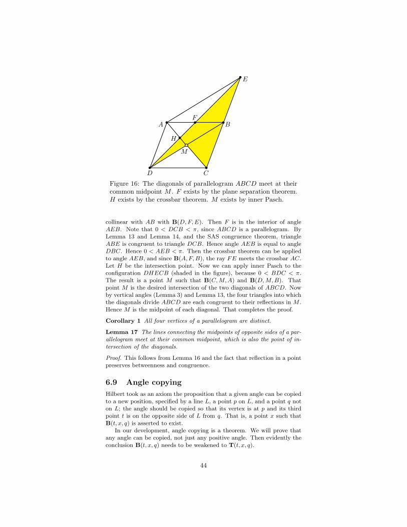
b

Db

C

bA

bE

bB

bF

M

bH

Figure 16: The diagonals of parallelogram ABCD meet at theircommon midpoint M . F exists by the plane separation theorem.H exists by the crossbar theorem. M exists by inner Pasch.

collinear with AB with B(D, F,E). Then F is in the interior of angleAEB. Note that 0 < DCB < π, since ABCD is a parallelogram. ByLemma 13 and Lemma 14, and the SAS congruence theorem, triangleABE is congruent to triangle DCB. Hence angle AEB is equal to angleDBC. Hence 0 < AEB < π. Then the crossbar theorem can be appliedto angle AEB, and since B(A,F,B), the ray FE meets the crossbar AC.Let H be the intersection point. Now we can apply inner Pasch to theconfiguration DHECB (shaded in the figure), because 0 < BDC < π.The result is a point M such that B(C,M,A) and B(D,M,B). Thatpoint M is the desired intersection of the two diagonals of ABCD. Nowby vertical angles (Lemma 3) and Lemma 13, the four triangles into whichthe diagonals divide ABCD are each congruent to their reflections in M .Hence M is the midpoint of each diagonal. That completes the proof.

Corollary 1 All four vertices of a parallelogram are distinct.

Lemma 17 The lines connecting the midpoints of opposite sides of a par-allelogram meet at their common midpoint, which is also the point of in-tersection of the diagonals.

Proof. This follows from Lemma 16 and the fact that reflection in a pointpreserves betweenness and congruence.

6.9 Angle copying

Hilbert took as an axiom the proposition that a given angle can be copiedto a new position, specified by a line L, a point p on L, and a point q noton L; the angle should be copied so that its vertex is at p and its thirdpoint t is on the opposite side of L from q. That is, a point x such thatB(t, x, q) is asserted to exist.

In our development, angle copying is a theorem. We will prove thatany angle can be copied, not just any positive angle. Then evidently theconclusion B(t, x, q) needs to be weakened to T(t, x, q).

44

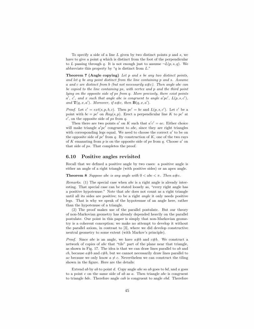
To specify a side of a line L given by two distinct points p and s, wehave to give a point q which is distinct from the foot of the perpendicularto L passing through q. It is not enough just to assume ¬L(p, s, q). Weabbreviate this property by “q is distinct from L.”

Theorem 7 (Angle copying) Let p and s be any two distinct points,and let q be any point distinct from the line containing p and s. Assumea and c are distinct from b (but not necessarily a#c). Then angle abc canbe copied to the line containing ps, with vertex and p and the third pointlying on the opposite side of ps from q. More precisely, there exist pointsa′, c′, and x such that angle abc is congruent to angle a′pc′, L(p, s, c′),and T(q, x, a′). Moreover, if a#c, then B(q, x, a′).

Proof. Let c′ = ext(s, p, b, c). Then pc′ = bc and L(p, s, c′). Let c′ be apoint with bc = pc′ on Ray(s, p). Erect a perpendicular line K to pc′ atc′, on the opposite side of ps from q.

Then there are two points a′ on K such that a′c′ = ac. Either choicewill make triangle a′pc′ congruent to abc, since they are right triangleswith corresponding legs equal. We need to choose the correct a′ to be onthe opposite side of pc′ from q. By construction of K, one of the two raysof K emanating from p is on the opposite side of ps from q. Choose a′ onthat side of ps. That completes the proof.

6.10 Positive angles revisited

Recall that we defined a positive angle by two cases: a positive angle iseither an angle of a right triangle (with positive sides) or an apex angle.

Theorem 8 Suppose abc is any angle with 0 < abc < π. Then a#c.

Remarks. (1) The special case when abc is a right angle is already inter-esting. That special case can be stated loosely as, “every right angle hasa positive hypotenuse.” Note that abc does not count as a right triangleuntil all its sides are positive; to be a right angle it only needs positivelegs. That is why we speak of the hypotenuse of an angle here, ratherthan the hypotenuse of a triangle.

(2) The proof makes use of the parallel postulate. But our theoryof non-Markovian geometry has already depended heavily on the parallelpostulate. Our point in this paper is simply that non-Markovian geome-try is a coherent conception; we make no attempt to develop it withoutthe parallel axiom, in contrast to [3], where we did develop constructiveneutral geometry to some extent (with Markov’s principle).

Proof. Since abc is an angle, we have a#b and c#b. We construct anetwork of copies of abc that “tile” part of the plane near that triangle,as shown in Fig. 17. The idea is that we can draw lines parallel to ab andcb, because a#b and c#b, but we cannot necessarily draw lines parallel toac because we only know a 6= c. Nevertheless we can construct the tilingshown in the figure. Here are the details:

Extend ab by ab to point d. Copy angle abc so ab goes to bd, and a goesto a point e on the same side of ab as a. Then triangle abc is congruentto triangle bde. Therefore angle cab is congruent to angle ebd. Therefore

45

b

ab

bb

db

m

b u

bℓ

b e

b fbv

bp

bq

c

Figure 17: Starting with abc with a#b and b#c, construct themidpoint m of ab and apply Pasch to prove B(a, c, f). Hencea#c.

segments ac and be are parallel (in the sense that if there are lines throughthose segments, they cannot meet, because that would contradict theexterior angle theorem). Angle cba is congruent to angle edb, so ed isparallel to cb. Since c#b and ed = cb, we have e#b, so we can extend deby de to a point f with ef = bc.

We have cb = ed and eb = be. Since ed is parallel to bc, the alternateinterior angles cbe and bed are equal. Hence, by SAS, triangle ceb iscongruent to triangle dbe. Then cedb is a quadrilateral with opposite sidesequal. Hence, by Lemma 15, it is a parallelogram. Hence, by Lemma 14,cd = bd = ab. By construction of f , ef = ed = bc. Hence, by SAS,triangle cef is congruent to triangle abc. Note, however, that we have notproved that a, c, and f lie on a line, and indeed the betweenness relationB(a, c, f) is what we are trying to prove, as that is one way to show a#c.We construct two more copies of triangle abc, by constructing a line vfthrough f parallel to ad and ce, with vf = ab and v on the same side of fas a, and extending df through f by bc to point u. Let m be the midpointof segment ab, which exists since a#b. Let ℓ be the midpoint of vf , whichexists since vf = ab and a#b, so v#f .

Angle bde is congruent to angle abc, because triangle cba is congruentto triangle edb. Since 0 < abc < π by hypothesis, we have 0 < bde < π.Hence we can apply inner Pasch to the configuration ufdam. The resultis a point k such that B(u, k,m) and B(a, k, f). In fact k = c, althoughwe have not proved that. Extending segments eb and uv, we get a largeparallelogram pueq as shown in the figure. The intersection of its diagonalsis at the midpoint of each diagonal, namely c. HenceB(u, c, q). Now a andf are midpoints of opposite sides of the parallelogram, so by Lemma 17,B(a, c, f). Then by definition, a#c. That completes the proof.

Theorem 9 Every positive angle is an apex angle.

Proof. A positive angle, by definition, is either an apex angle, or a rightangle, or an angle of a right triangle. If it is an apex angle, there is nothing

46

to prove.A right angle is an apex angle, since given a right angle, we can lay

off the same distance on each of its sides, constructing a right isoscelestriangle. By Theorem 8, the base of this triangle has distinct endpoints,and hence, it has a midpoint. That makes the right angle an apex triangle.

It remains to prove that every angle of a right angle is an apex angle.Let acb be a right triangle with the right angle at c. Fig. 18 illustratesthe proof.

ba

bc

b

db

bFigure 18: Angle abc is an apex angle, because a#d as the hy-potenuse of right angle acd.

According to Lemma 9, ac < ab. By definition of triangle, a#c. Let ebe the reflection of c in b, so B(e, b, c) ∧ eb = ec. (e is not shown in thefigure.) Then by Lemma 4, there is a unique point d with B(e, b, d) andbd = ab. By Lemma 9, bc < ab. Hence bc < bd. By definition of <, thereexists a point c′ with B(b, c′, d) and bc′ = bc. We have B(b, c′, d) andB(e, b, d). Applying inner transitivity (Axiom A15-i), we have B(e, b, c′).Now we have B(e, b, c′) ∧ bc′ = bc, and also B(e, b, c) ∧ bc = bc. By theuniqueness part of Lemma 4, c = c′. Since B(b, c′, d) we have B(b, c, d).Therefore c#d. Now acd is a right triangle since acb is a right angle, andboth legs cd and ac have distinct endpoints. Applying Theorem 8 to rightangle acd, we obtain a#d. Since ba = bd, this proves abc is an apex angle,as desired. That completes the proof.

Theorem 10 (Angle bisection) Every positive angle can be bisected.

Proof. Let abc be a positive angle. Then by Theorem 9, abc is an apexangle. That is, there are points u, v on Ray(b, a) and Ray(b, c) respectivelysuch that bu = bv and u#v. Since u#v, Theorem 5 implies that uv hasa midpoint, say m. By Theorem 8, since b#u and u#m, we have b#m.Hence bmu and bmv are triangles. Since um = vm, angle ubv is bisectedby Ray(b,m). Since angle abc is the same angle as ubv, angle abc isbisected by Ray(b,m). That completes the proof.

Remark. Euclid’s Proposition I.9 purports to prove that every anglecan be bisected; but the proof has more than one flaw. First, if the angleto be bisected is equilateral, the two points determining Euclid’s bisectormight coincide, and thus fail to determine a line. Second, without anydimension axiom, the equilateral triangle produced by applying I.1 in theproof of I.9 might lie in a different plane from the angle to be bisected, thusthe “bisector” would fail to lie in the plane of the angle. These difficultiesare not easy to repair, especially without using a dimension axiom; but

47

it is done as above, by using Gupta to find the midpoint of the base ofan equilateral triangle, and then using inner Pasch. In other words, theabove approach, which we use here in non-Markovian geometry, is (as faras I know) actually the simplest way to repair Euclid I.9. Of course, if wedo not care about avoiding Markov’s principle, some of the complicationsfall away.

7 Geometric arithmetic without Markov’s

principle

In [4, 3], we showed that in EG plus Markov’s principle, one can definecoordinates, and one can define addition and multiplication of points on afixed line. The constructions differ from the classical ones because we needto avoid a case distinction according to the signs of the arguments. Twoways of defining addition and multiplication constructively are studied inthe cited paper. One is purely geometrical, in which addition is definedusing uniform rotation and reflection, and multiplication is defined usinga circle, following Hilbert. We have checked that Markov’s principle is notused in these constructions and proofs in any essential way. Actually, wefound only one place where it was used, and we fixed that by providing inthis paper a non-Markovian proof of Lemma 12. In the discussion below,we will point out how that lemma is used.

7.1 Coordinates

Once we have the uniform perpendicular, it is possible to define coordi-nates. Pick two perpendicular lines to serve as the x-axis and the y-axis.Then to each point p we can assign the feet a and b of the perpendic-ulars through p to the x-axis and y-axis, respectively. Then a is thex-coordinate of p. To get the y-coordinate, however, we must rotate b by90◦, because the y-coordinate is supposed to be a point on the x-axis, thesame distance from the origin as b. Therefore we need to define uniformrotation; “uniform” in the sense that it works without a case distinctionas to the sign of b. A rotation by 90◦ is equivalent to two reflections inthe line y = x; so it suffices to define uniform reflection.

The final step in the construction of coordinates is to show that, givenpoints x and y on the x-axis, we can construct a point P (x, y) whosecoordinates are (x, y). Namely, erect a perpendicular J to the x-axis atx on the opposite side of the x-axis from (0,−1). (The theorem abouterecting perpendiculars requires a point not on the line, and then theperpendicular is constructed on the opposite side of the line from thatpoint. This guarantees that J lies in the plane of the two axes. Rotatey counterclockwise about the origin by 90◦ (in the plane of the two axes,i.e., using the two axes to define the angle of rotation) to a point q. Dropa perpendicular from q to J . The foot of that perpendicular is P (x, y).But why are the coordinates of P (x, y) equal to (x, y)? Let p = P (x, y)and let 0 be the origin. By construction the quadrilateral qpx0 has rightangles at p,x, and 0; it is therefore a Lambert quadrilateral (three right

48

angles). It lies in the plane determined by the two axes since the points pand q are on the opposite side of the x-axis from (0,−1).

Using the parallel postulate, we prove every Lambert quadrilateral ina plane is a rectangle. Hence the angle at q is also a right angle; henceq is the foot of the perpendicular from p to the y-axis; hence y is they-coordinate of p, as claimed.

Thus the construction of coordinates depends on the theorem thatevery planar Lambert quadrilateral is a rectangle (a quadrilateral withfour right angles). We claim that this theorem can be proved, withoutusing Markov’s principle, from the weakest form of the parallel postu-late (Playfair’s axiom). It is mentioned in Lemma 5.24 of [4], but theproof is not given there. In [3], Lemma 10.2, it is proved in intuitionisticTarski geometry that a planar Saccheri quadrilateral is a rectangle. (ASaccheri quadrilateral is a quadrilateral abcd with right angles at b and cand ab = cd.) Half a Saccheri quadrilateral is a Lambert quadrilateral,and a Lambert quadrilateral can be doubled to make a Saccheri quadri-lateral, so the cited lemma implies that a planar Lambert triangle is arectangle, as desired. The proof of that theorem given in [3] is almostfree of Markov’s principle, but it does appeal to Lemma 12 (in the num-bering of the present paper), which in the cited paper is proved usingMarkov’s principle. However, in this paper we proved Lemma 12 withoutusing Markov’s principle. Hence, the uniqueness of coordinates is provedwithout using Markov’s principle.

7.2 Euclidean fields without Markov’s principle

In [4], we gave axioms for (intuitionistic) Euclidean fields. The languagehas constants 0 and 1, function symbols +, −, ·, 1/x or x−1 for multi-plicative inverse, and

√, and a predicate P (x) for “x is positive.” The

axioms are the field axioms, the axioms for order (involving P ), and theaxiom that non-negative elements have square roots. In addition we tookMarkov’s principle ¬¬P (x) → P (x) as an axiom.

Now we want to drop Markov’s principle. When Markov’s principleis allowed, non-zero elements have multiplicative inverses if and only ifpositive elements have inverses, since 1/x = x/|x|, where |x| =

√x2. This

argument works if |x| is positive when x is nonzero, but that is equivalentto Markov’s principle. In the absence of Markov’s principle, then, theaxiom that positive elements have multiplicative inverses does not implythat all nonzero elements have multiplicative inverses, and we leave thataxiom unmodified.

Models of the resulting theory will be called “weakly Euclidean fields”,since we already used “Euclidean fields” for models that satisfy Markov’sprinciple. To be precise, the axioms are the usual axioms of commutativering theory, plus the following:

¬x 6= y → x = y stability of equality

0 6= 1 EF0

P (x) → ∃y (x · y = 1 ∧ P (y)) EF1

P (x) ∧ P (y) → P (x+ y) ∧ P (x · y) EF2

49

x+ y = 0 → ¬(P (x) ∧ P (y)) EF3

x+ y = 0 ∧ ¬P (x) ∧ ¬P (y) → x = 0 EF4

x+ y = 0 ∧ ¬P (y) → ∃ z(z · z = x) EF5

Equivalently one may express EF1 and EF5 using the function symbols1/x and

√x, achieving thereby a quantifier-free axiomatization; and if

one does not like using a function symbol for a not-everywhere-definedfunction, one may use the Logic of Partial Terms (LPT), as explained in[3]. Note that EF1 requires that the inverse positive element not onlyexist but also be positive itself. If Markov’s principle is allowed, one canprove that the inverse of a positive element is positive, but since we arenot assuming Markov’s principle, that cannot (as it turns out) be proved,and we assume it as part of EF1.

Let F be an ordered field. Then “the plane over F”, denoted by F2, is

a geometrical structure determined by defining relations of betweennessand equidistance in F

2, using the given order of F. Namely, b is betweena and c if it lies on the interior of the segment ac. That relation canbe expressed more formally in various ways, for example (using the crossproduct) by (c− b)× (b− a) = 0 and (b− c) · (a− b) > 0.

The equidistance relation E(a, b, c, d), which means that segment ab iscongruent to segment cd, can be defined by (b− a)2 = (d− c)2. Note thatno square roots were used, so these definitions are valid in any orderedfield.

The cross product u × v is defined using components as usual. Ifthe lines through uv and st intersect (and do not coincide), then usingCramer’s rule, the formula for the intersection point has denominatorgiven by the cross product D = (t − s) × (v − u). (Details are in §9.3 of[4].) So, in verifying inner Pasch and outer Pasch, we will need to knowthat the cross products for the lines that need to intersect are positive.Thus what has to be proved is the following lemma:

Lemma 18 In F2, the cross product (in the sense defined above) of the

vectors giving the sides of angle abc with 0 < abc < π is positive. Inparticular, if d lies on ab, then |d − c| > 0, and if ab lies on the x-axis,then |c2| > 0.

Remark. At the end, the proof requires the modified EF1, which says thatinverses of positive elements are positive.

Proof. By a rotation and translation, we can assume that b = (0, 0) anda lies on the positive x-axis. (All three cases in the definition of “posi-tive angle” are invariant under rotation and translation.) Then the crossproduct in question is a × c = c2a1. Since a1 > 0, the cross product haspositive absolute value if and only if |c2| > 0. The penultimate statementfollows from c2 > 0, since |d − c| is the hypotenuse a right triangle witha vertical leg of length c2, and in F

2 the theorem that a leg of a righttriangle is shorter than the hypotenuse holds.

Assume 0 < abc < π. If angle abc is a right angle or an angle of aright triangle, |v2| > 0 is immediate. So we may assume abc is an apexangle. Then there are distinct points u = (u1, 0) and v on the ray from(0, 0) through c, such that u1 > 0 and |u| = |v|. We have |u− v| > 0 since

50

u and v are distinct. The cross product of the two sides of the angle isu× v = u1v2, since u2 = 0. We must show |u1v2| > 0. Since u1 > 0, thatis equivalent to v2 > 0. We have not yet used the assumption abc < π,which we will now need. Let d = (−a1, 0). Then 0 < dbc, by definition ofabc < π. There are three cases: dbc is an apex angle, a right angle, or anangle of a right triangle. If either of the latter two then c2 > 0, so v2 > 0and we are done. So we may assume dbc is an apex angle. Then there aredistinct points p and q on the negative x-axis and bc, respectively, suchthat |p| = |q| and |p| > 0. Extending the positive-length vectors u and v by|p| and the vectors p and q by |u|, we can assume without loss of generalitythat |u| = |p| = |v| = |q. Then v = q and angle pqu = pvu is inscribed inthe semicircle pvu with center at b = (0, 0). Since classically F

2 satisfiesthe theorem that an angle inscribed in a semicircle is a right angle, andbeing a right angle is equationally described, pvu is a right angle. |p2|is the altitude of that right triangle. By Lemma 18, F2 satisfies that thealtitude of a right triangle (with positive legs) is positive. Hence |p2| > 0.But c2/|c| = p2/|p|, and 1/|c| and 1/|p| are both positive by EF1, since|c| > 0. Hence c2 is a positive quantity times p2. Hence |c2| > 0, asdesired. That completes the proof of the lemma.

The following theorem verifies that we have the axioms for weaklyEuclidean fields right.

Theorem 11 Every plane F2 over a weakly Euclidean field F is a model

of Euclidean geometry EG.

Remark. This theorem depends on the modifications we made to theextension axiom and to inner and outer Pasch; had we not changed theformulations of inner and outer Pasch to require an angle to be positiveand have a positive supplement, we would need Markov’s principle toverify them. Although these calculations are elementary, we need to verifythat Markov’s principle is not necessary, and that we only need to divideby elements that are known to be positive, and we need square roots onlyof positive elements (as opposed to nonzero elements). The fact that thesecalculations succeed without Markov is a strong indication that we havethe axioms of EG right.

Proof. We define x > y to abbreviate P (y − x) and x ≥ y to abbreviate¬x < y, and similarly for < and ≤. We prove the transitivity of <.Suppose x < y and y < z. Then P (y − x) ∧ P (z − y). By EF2, P ((y −x) + (z − y)). Hence P (z − x). Hence x < z.

We define absolute value in F2:

|(x, y)| :=√

x2 + y2.

We have x2 ≥ 0 for all x (for example, since ≤ is stable, we can provethat by contradiction). Hence |u| is always defined.

The interpretation of betweenness in F2 has to be given without using

cases. Collinearity L(u, v, w) can be defined by

L(u, v, w) := (w − u)× (w − v) = 0.

Then betweenness is defined by

B(u, v, w) := L(u, v, w)∧|v−u|+|w−v| = |w−u|∧|v−u| > 0∧|w−v| > 0.

51

Since translations and rotations are given by linear maps with determi-nant one, they preserve cross and dot products, and hence they preservedistance and collinearity, and hence they preserve betweenness as well.

We claim that two points u and v in F2 are distinct if and only if

|v − u| > 0. According to the definition of u#v, u and v are distinct ifthere is a point x bearing any of the three possible betweenness relationswith u and v. For example, suppose B(u, x, v). Then by the definition ofbetweenness, |x − u| > 0 and |v − x| > 0 and L(u, x, v). We must show|v − u| > 0. By a rotation and translation, we may assume u = (0, 0)and x = (x1, 0) and y = (y1, 0). Then we have x1 > 0 and y1 > x1, andwe must show y1 > 0; but that is the transitivity of >, which we provedabove. Similarly for the other two possible betweenness relations. Thusu#v if and only if |v − u| > 0.

We turn to the betweenness axioms. Consider the axiom ¬B(a, b, a).In F

2, we have B(a, b, c) → L(a, b, c), by the definition of B(a, b, c). Sup-pose B(a, b, a). Then L(a, b, a). By a rotation and translation, we can as-sume a and b lie on the x-axis. ThenB(a, b, a) becomes |b2−a2|+|a2−b2| =|a2−a2|. But the last expression is 0. With x = b2−a2, we have 2|x| = 0.Hence x = 0; that is, b2 = a2. Hence a = b. But that contradictsB(a, b, a). Hence our assumption B(a, b, a) is contradictory. That is,¬B(a, b, a), which is what had to be proved.

Consider the symmetry of betweenness, B(a, b, c) → B(c, b, a). Sup-pose B(a, b, c); after a rotation and translation, we can assume a, b, and clie on the x-axis. For simplicity we drop subscripts, writing just a insteadof a1, etc. Then we have |c − b| + |b − a| = |c − a| and |c − b| > 0 and|b− a| > 0. What has to be proved is an equation representing non-strictbetweenness T(c, b, a) and the two inequalities |a− b| > 0 and |b− c| > 0.By the stability of equality, we can argue classically for the non-strict be-tweenness, which we take as proved. The two inequalities follow from theeasy lemma | − x| = |x|. That completes the verification of the symmetryof betweenness.

Consider the inner transitivity of betweenness, axiom A15-i:

B(a, b, d) ∧B(b, c, d) → B(a, b, c).

Suppose the hypothesis. Again we can apply a rotation and translationto bring all the points to the x-axis. As before the non-strict inequalityT(a, b, c) is expressed by an equation, so by the stability of equality, wecan prove it classically, which we assume done. For simplicity we dropthe subscripts, writing just a instead of a1, etc. Then a ≤ b ≤ c ≤ d. Wehave a < b < d and b < c < d by hypothesis. We need to prove a < b < c.But we have both inequalities already; there is no existential assertion toprove. That completes the verification of the inner transitivity axiom.

Next we turn to the inner Pasch axiom. Please refer to Fig. 8. By arotation and translation, and possibly renaming some of the points, wemay assume aq lies on the x-axis and c2 ≥ 0 and q1 ≥ a1. We haveto show that |(q − a) × (b − p)| > 0. That is, |(b2 − p2)(q1 − a1)| > 0.The hypothesis of inner Pasch includes the specification that either anglebca or angle pqb is between 0 and π. First assume 0 < bca < π. ByLemma 18, applied to angle bca, any point on bc is at a positive distance

52

from a. Hence |a − q| > 0. Hence q1 − a1 > 0. Therefore by EF1,1/(q1 − a1) > 0. Hence it suffices to show |b2 − p2| > 0. Because B(c, q, b)holds by hypothesis, we have |c− q| > 0, so acq is an angle, and the sameangle as acb. Since being positive respects the same-angle relation, andeven angle congruence, 0 < acq < π. Then by Lemma 18, c lies at positivedistance from aq. That is, c2 > 0. Therefore b2 < 0, since B(b, q, c) andq2 = 0. Because B(a, p, c) holds by hypothesis and c2 > 0 and a2 = 0, wehave p2 > 0. Now we have b2 < 0 < p2. Hence |b2 − p2| > 0, as desired.That completes the verification of inner Pasch, in the case 0 < bac < π.We note that it would not work without Markov’s principle if we had onlyT(c, q, b) for a hypothesis instead of B(c, q, b).

It remains to verify inner Pasch under the assumption 0 < qpa < πinstead of 0 < bca < π. Then Lemma 18 tells us that |(q− p)× (a− p)| >0. We are free to choose the origin of coordinates so that p1 = 0 anda2 = q2 = 0. Then

|(q1 − p1)(a2 − p2)− (q2 − p2)(a1 − p1)| > 0

| − q1p2 − (−p2)(a1)| > 0

|p2(a1 − q1)| > 0.

By Lemma 18, |a1 − q1)| > 0. Hence p2 > 0. Since B(a, p, c), that impliesc2 > 0. That in turn implies |(a− c)× (q− c)| > 0, which in turn implies|(a− c)× (q − ℓ)| > 0, for any point ℓ on the ray cq; in particular for thepoint ℓ such that |ℓ−c| = |a−c|. Hence 0 < acb < π. But we have alreadyverified that under that hypothesis, inner Pasch holds, so that completesthe verification of inner Pasch.

Now we turn to outer Pasch. We may assume a = (0, 0) and q = (q1, 0),so aq lies on the x-axis. As with inner Pasch, the crucial issue is to verifythat the lines that need to intersect have positive cross product. Forouter Pasch that is |(q − a) × (b − p)|, which is |q1 − a1| |b2 − p2|. Since0 < baq < π ∨ 0 < abq < π, q and a are distinct points, so q1 > a1,and b2 > 0. Hence |q1 − a1| > 0, and to finish the verification it sufficesto prove |b2 − p2| > 0. Since B(b, c, q), we have 0 < c2 < b2, and sinceB(a, p, c) we have 0 < p2 < c2. Hence 0 < p2 < b2. That completes theverification of outer Pasch.

Any axiom whose analytic-geometry interpretation does not involvea positive occurrence P (x) will be automatically verifiable, by Godel’sdouble-negation interpretation. That is, starting with the classical veri-fication, we just push double negations inwards, and when they reach anequality, we drop them by the stability of equality, and the result is anintuitionistic verification. If the statement had a positive occurrence ofP (x) we would need Markov’s principle to drop the double negation, but anegative occurrence causes no problem. If the statement does not involveP (x), the need does not arise. On these grounds, the 5-segment axiom,line–circle continuity and circle–circle continuity (which have occurrencesof P (x), counting as negative by virtue of being in the hypotheses) holdin F

2. (See [4] for a more detailed discussion.)The dimension axioms (once properly formulated) are easily verified

in F2. That completes the proof of the theorem.

53

8 Geometric arithmetic

We have already discussed the construction of coordinates relative to apair of perpendicular lines chosen as axes. The definitions of multipli-cation and addition for positive arguments then offers no difficulty. Forexample, the multiplicative inverse of a point (a, 0) on the x-axis is foundby erecting a perpendicular to the x-axis at the point 1, and using Euclid5 to prove that it meets the line containing the line through (0, 0) and(a, 1). That point has coordinates (1, 1/a). To use the non-Markovianversion of Euclid 5, we need the hypothesis that point (a, 0) is distinctfrom (0, 0). The passage from signed to unsigned multiplication is dis-cussed in [4], where two solutions are given. For example, the solution byusing Hilbert’s definition of multiplication using a circle works in EG (butit does require the non-strict version of line–circle continuity, which weincluded partly for that reason). It follows that, loosely speaking, “everymodel of EG is a plane over a Euclidean field.”

9 Some results about EG

In this section we present some metamathematical results about non-Markovian geometry EG.

9.1 A Kripke model of non-Markovian geometry

We want to demonstrate that non-Markovian geometry is “about some-thing” by giving a model of it in which Markov’s principle fails. Of course,we cannot give a model in the classical sense, since the double negationof Markov’s principle is a theorem. But we can give a two-node Kripkemodel. (For an introduction to Kripke models and a proof of the complete-ness theorem, see [29], Part V, pp. 324ff. Since our model is particularlysimple, you may be able to understand it without a background in Kripkemodels.)

In view of the fact that non-Markovian geometry is interpretable inthe theory of Euclidean fields (without Markov’s principle), it suffices togive a Kripke model that does not satisfy Markov’s principle of Euclideanfield theory in the form ¬¬P (x) → P (x). Then a corresponding model ofEG can be constructed by replacing each field Fα in the first Kripke modelby the plane F

2

α over Fα, with betweenness and congruence interpreted asin the previous section.

Theorem 12 Euclidean field theory does not imply Markov’s principle,and geometry EG does not imply Markov’s principle.

Proof. The second claim follows from the first and Theorem 11. We willconstruct a Kripke model of Euclidean field theory in which MP fails. LetF be any non-Archimedean field (so it contains some “infinite” element,larger than any positive integer). Let F0 be the set of “finitely bounded”elements of F, i.e., those elements bounded by some positive integer. F0

contains “infinitesimal” elements x, by definition those whose reciprocalsare not finitely bounded. We interpret P (x) in F0 to mean that x is

54

positive in F and not infinitesimal. Then F0 is not a classical model ofEuclidean ordered field theory, but it is still admissible as a node in aKripke model.

The definition of a Kripke model includes these two clauses: Mα|=¬φmeans that φ fails everywhere above α, and Mα|=A → B means that ifMβ |=A for β > α, then Mβ|=B. The soundness theorem (easy to check)for Kripke models says that the satisfaction relation preserves intuitionis-tic logical consequence. Hence, to prove that Markov’s principle is not atheorem of Euclidean field theory, it suffices to exhibit a Kripke model inwhich Markov’s principle is not satisfied. That Kripke model, call it M,will be a two-node model. The root node M0 has universe F0, but P (x)is interpreted in M0 to mean that x is positive in F and not infinitesimal.The other node, lying “above” M0, is M1, which is the classical modelF.

We now show that Markov’s principle fails in M. Let x be infinitesimalin F. Then the root node M0 satisfies ¬¬P (x), since x is positive in F,and satisfaction in M1 is just classical satisfaction. Suppose, for proof bycontradiction, that M satisfies Markov’s principle. Then the root nodesatisfies the hypothesis ¬¬P (x) of Markov’s principle, so it must satisfythe conclusion P (x). But, by definition of P in M0, that implies x is notinfinitesimal, contradiction. Hence Markov’s principle does not hold inM.

We still need to check that the axioms of Euclidean field theory holdin M. Since satisfaction at node M1 is just classical satisfaction, we onlyneed to check M0.

Consider EF0: ¬x 6= y → x = y. Suppose M0 satisfies ¬x 6= y. ThenM1 does not satisfy x 6= y. Hence x = y in F. Hence x = y in F0. HenceM satisfies EF0.

Consider EF1: P (x) → ∃y (x · y = 1). Suppose M0|=P (x). Then xis positive and not infinitesimal. Hence y = 1/x in F is finitely bounded,so it belongs to F0. Hence x has an inverse in F0. EF1 also requires thatinverse to be positive, which it is, since it is positive in F. Therefore M0

satisfies EF1.Consider EF2: P (x)∧P (y) → P (x+y)∧P (x·y). SupposeM0|=P (x)∧

P (y). Then x and y are positive and not infinitesimal. Then their sumand product are positive. Since x is not infinitesimal, by definition 1/x isfinitely bounded. Let n be an integer such that 1/x < n. Then

1

x+ y<

1

x< n.

Hence 1/(x+ y) is finitely bounded. Hence x+ y is positive in M0. Also

1

xy=

1

x

1

y< nm

provided 1/y < m. Hence xy is also positive in M0. Hence M0 satisfiesEF2.

Consider EF3: x+ y = 0 → ¬(P (x)∧ P (y)). Suppose x+ y = 0 holdsin M0 and P (x)∧P (y) holds in M0 or in M1. Then x and y are positivein F, contradicting the fact that F satisfies EF3. Hence M satisfies EF3.

55

Consider EF4: x + y = 0 ∧ ¬P (x) ∧ ¬P (y) → x = 0. SupposeM0|=¬P (x). Then M1 does not satisfy P (x), so x is not positive inF. If the same is true of y = −x, then since F classically satisfies EF4,x = 0. Hence M0 satisfies EF4.

Consider EF5, namely x + y = 0 ∧ ¬P (y) → ∃ z(z · z = x). SupposeM0 satisfies x+ y = 0 ∧ ¬P (y). Then y = −x is not positive in F, so byEF5 in F, x has a square root z in F. We claim z is finitely bounded, andhence lies in F0. If |z| < 1 we are done. Otherwise, let n be an integergreater that |x|; then |z| ≤ √

n < n+ 1. That completes the proof of thetheorem.

Remark. In the corresponding geometrical Kripke model, whose twonodes are M0 = F 2

0 and M1 = F 2

1 , with betweenness and congruencedefined in the obvious way (details in [4]), two points of M0 are distinct ifand only if the difference of both their coordinates is infinitesimal, and anangle is positive if and only if the rays that form its sides contain pointsat equal distances from the vertex that are distinct; loosely speaking, theangle is not infinitesimal. This model is in accord with the intuition thatif Markov’s principle does not hold, one has to imagine that every pointhas a “cloud” of nearby points, infinitesimally close to it but not equal;so near that the two points cannot determine a line.

Remark. This model, and another more complicated model, were givenin [4], to show that Markov’s principle does not follow from EF0–EF5.But it was not appreciated at the time that Markov’s principle does fol-low from the axioms of constructive geometry, unless the extension axiomand Pasch’s axiom(s) are modified by requiring distinct points and posi-tive angles; geometry without Markov’s principle was purposely not dealtwith in [4], since “sufficient to the day are the tribulations thereof.” Inother words, the difficulties of non-Markovian geometry then seemed in-timidating, and were postponed.

9.2 EG is not too weak

We created the theory EG by starting with constructive geometry from [4],removing Markov’s principle, and modifying the segment extension andPasch axioms. We now show that we have not made EG too weak, in thesense that if we add Markov’s principle back to EG, we also automaticallyget back the unmodified axioms of constructive geometry.

Lemma 19 EG plus Markov’s principle proves that any two unequal pointsare distinct, and if a, b, c are not collinear, then 0 < abc < π.

Proof. Let a 6= b. Let α#β (two such points exist by the lower dimensionaxiom of EG). Extend αβ by ab to point e. Then T (α,β, e). Since a 6= band ab = βe, we have β 6= e. With Markov’s principle, we have B(x, y, z)equivalent to T(x, y, z) ∧ x 6= y ∧ y 6= z. Hence, with Markov’s principle,B(α, β, e). Hence β#e. Then ab is congruent to the positive segmentβe. Hence it can be extended by cd to a new point f , using the segmentextension axiom of EG. Then B(a, b, f). Then by definition a#b.

Now suppose ¬L(a, b, c). We will prove 0 < abc < π. Since ¬L(a, b, c),we have a 6= b and b 6= c, and using Lemma 4, we can assume without

56

loss of generality that ab = bc. Since ¬L(a, b, c) we have a 6= c. As shownabove, Markov’s principle then implies a#c, so 0 < abc. Let d be thereflection of c in b; then similarly, 0 < abd, so abc < π. That completesthe proof of the lemma.

Theorem 13 EG plus Markov’s principle proves the axioms of construc-tive Tarski geometry given in [4].

Proof. We will prove the segment extension axiom A4, which says thatif a 6= b then ab can be extended by any segment cd. By Lemma re-flemma:nottooweak, with Markov’s principle a 6= b implies a#b, so thesegment extension axiom of EG applies. That completes the proof ofaxiom A4.

Next, we will verify the (unmodified) inner Pasch axiom. In con-structive geometry, the hypotheses include ¬L(a, b, c). By Lemma 19,0 < abc < π. Then the inner Pasch axiom of EG can be applied. Thatcompletes the verification of inner Pasch.

The dimension axiom of EG immediately implies the dimension ax-iom of constructive geometry, and no other axioms were modified. Thatcompletes the proof of the theorem.

9.3 EG is strong enough

In this section we advance the following principle

If, in any theorem of Euclidean geometry of the type found inBooks I-IV, we replace “a and b are unequal” by “a and b aredistinct”, and we require that all angles be positive, then theresulting theorem is provable in non-Markovian geometry EG.

The first difficulty here is “of the type found in Books I-IV.” The principlesurely fails if the theorem in question is Markov’s principle itself. ButMarkov’s principle is not a proposition of the kind found in Euclid. Asdiscussed above, those propositions are “Horn formulas”; that is, theirhypotheses are atomic statements (possibly involving defined concepts)and some given points, and the conclusions assert the existence of somepoints bearing positive relations to the original points.

A second difficulty is that the language of EG does not mention “an-gles” directly, so what exactly is meant by “require that all angles bepositive”? The phrase “angle abc” means (in ordinary geometry) thatthe three points are distinct and not collinear. We call a formula φ “ofEuclidean form” if it is expressed as a Horn formula in a language ex-tending EG by a 3-ary predicate Angle and a 2-ary predicate D, whereD occurs only negatively (that is, in the antecedent of the implication).Then the “ordinary interpretation” of φ is obtained by replacing D(a, b)by a 6= b and Angle(a, b, c) by ¬L(a, b, c). The “non-Markovian inter-pretation” is obtained by replacing D(a, b) by a#b and Angle(a, b, c) by0 < abc < π, both of which are abbreviations for existential formulas ofEG. The existential quantifiers in the antecedent are then pulled out, sothat the non-Markovian interpretation of φ has additional free (or univer-sally quantified) variables. Now we are able to state a theorem:

57

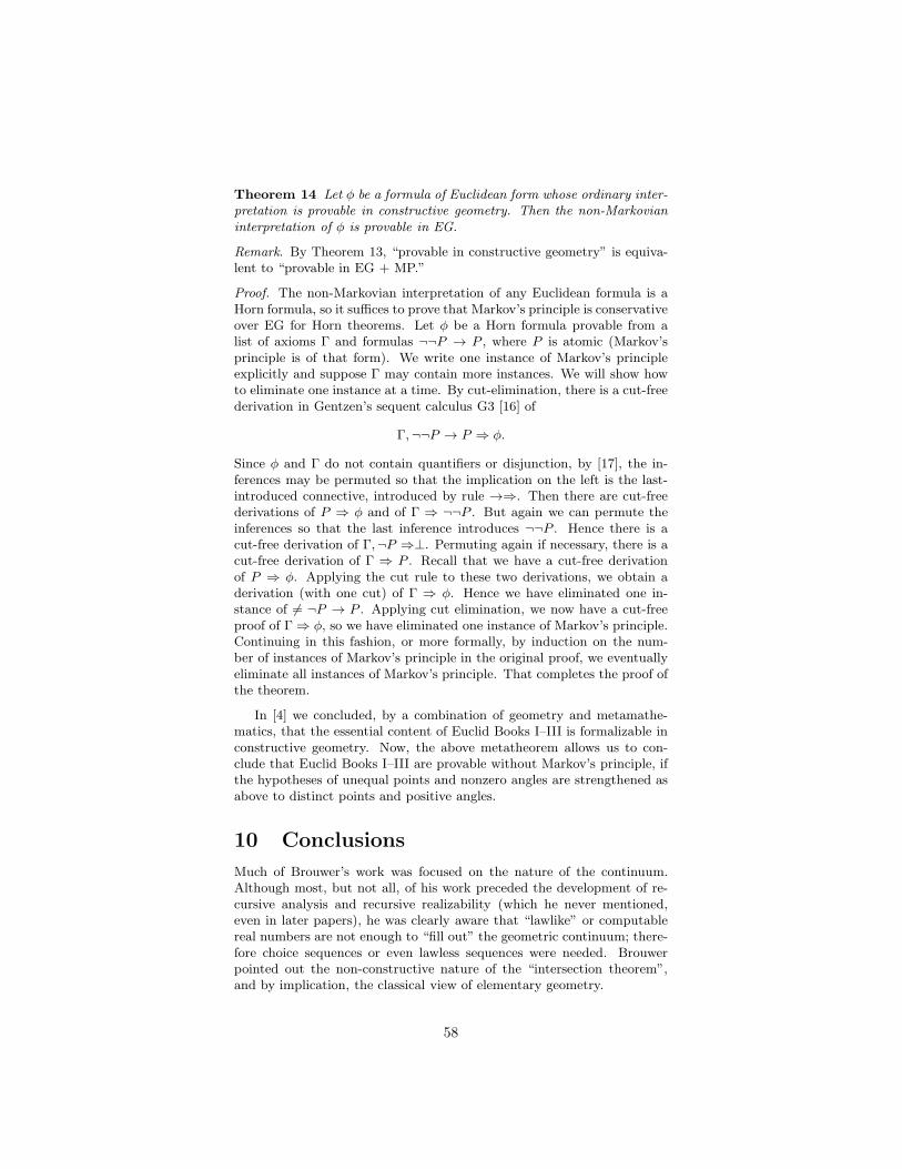
Theorem 14 Let φ be a formula of Euclidean form whose ordinary inter-pretation is provable in constructive geometry. Then the non-Markovianinterpretation of φ is provable in EG.

Remark. By Theorem 13, “provable in constructive geometry” is equiva-lent to “provable in EG + MP.”

Proof. The non-Markovian interpretation of any Euclidean formula is aHorn formula, so it suffices to prove that Markov’s principle is conservativeover EG for Horn theorems. Let φ be a Horn formula provable from alist of axioms Γ and formulas ¬¬P → P , where P is atomic (Markov’sprinciple is of that form). We write one instance of Markov’s principleexplicitly and suppose Γ may contain more instances. We will show howto eliminate one instance at a time. By cut-elimination, there is a cut-freederivation in Gentzen’s sequent calculus G3 [16] of

Γ,¬¬P → P ⇒ φ.

Since φ and Γ do not contain quantifiers or disjunction, by [17], the in-ferences may be permuted so that the implication on the left is the last-introduced connective, introduced by rule →⇒. Then there are cut-freederivations of P ⇒ φ and of Γ ⇒ ¬¬P . But again we can permute theinferences so that the last inference introduces ¬¬P . Hence there is acut-free derivation of Γ,¬P ⇒⊥. Permuting again if necessary, there is acut-free derivation of Γ ⇒ P . Recall that we have a cut-free derivationof P ⇒ φ. Applying the cut rule to these two derivations, we obtain aderivation (with one cut) of Γ ⇒ φ. Hence we have eliminated one in-stance of 6= ¬P → P . Applying cut elimination, we now have a cut-freeproof of Γ ⇒ φ, so we have eliminated one instance of Markov’s principle.Continuing in this fashion, or more formally, by induction on the num-ber of instances of Markov’s principle in the original proof, we eventuallyeliminate all instances of Markov’s principle. That completes the proof ofthe theorem.

In [4] we concluded, by a combination of geometry and metamathe-matics, that the essential content of Euclid Books I–III is formalizable inconstructive geometry. Now, the above metatheorem allows us to con-clude that Euclid Books I–III are provable without Markov’s principle, ifthe hypotheses of unequal points and nonzero angles are strengthened asabove to distinct points and positive angles.

10 Conclusions

Much of Brouwer’s work was focused on the nature of the continuum.Although most, but not all, of his work preceded the development of re-cursive analysis and recursive realizability (which he never mentioned,even in later papers), he was clearly aware that “lawlike” or computablereal numbers are not enough to “fill out” the geometric continuum; there-fore choice sequences or even lawless sequences were needed. Brouwerpointed out the non-constructive nature of the “intersection theorem”,and by implication, the classical view of elementary geometry.

58

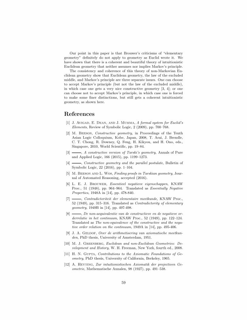
Our point in this paper is that Brouwer’s criticisms of “elementarygeometry” definitely do not apply to geometry as Euclid wrote it. Wehave shown that there is a coherent and beautiful theory of intuitionisticEuclidean geometry that neither assumes nor implies Markov’s principle.

The consistency and coherence of this theory of non-Markovian Eu-clidean geometry show that Euclidean geometry, the law of the excludedmiddle, and Markov’s principle are three separate issues. One can chooseto accept Markov’s principle (but not the law of the excluded middle),in which case one gets a very nice constructive geometry [3, 4]; or onecan choose not to accept Markov’s principle, in which case one is forcedto make some finer distinctions, but still gets a coherent intuitionisticgeometry, as shown here.

References

[1] J. Avigad, E. Dean, and J. Mumma, A formal system for Euclid’sElements, Review of Symbolic Logic, 2 (2009), pp. 700–768.

[2] M. Beeson, Constructive geometry, in Proceedings of the TenthAsian Logic Colloquium, Kobe, Japan, 2008, T. Arai, J. Brendle,C. T. Chong, R. Downey, Q. Feng, H. Kikyou, and H. Ono, eds.,Singapore, 2010, World Scientific, pp. 19–84.

[3] , A constructive version of Tarski’s geometry, Annals of Pureand Applied Logic, 166 (2015), pp. 1199–1273.

[4] , Constructive geometry and the parallel postulate, Bulletin ofSymbolic Logic, 22 (2016), pp. 1–104.

[5] M. Beeson and L. Wos, Finding proofs in Tarskian geometry, Jour-nal of Automated Reasoning, accepted (2016).

[6] L. E. J. Brouwer, Essentieel negatieve eigenschappen, KNAWProc., 51 (1948), pp. 964–964. Translated as Essentially NegativeProperties, 1948A in [14], pp. 478-840.

[7] , Contradictoriteit der elementaire meetkunde, KNAW Proc.,52 (1949), pp. 315–316. Translated as Contradictority of elementarygeometry, 1949B in [14], pp. 497-498.

[8] , De non-aequivalentie van de constructieve en de negatieve or-derrelatie in het continuum, KNAW Proc., 52 (1949), pp. 122–124.Translated as The non-equivalence of the constructive and the nega-tive order relation on the continuum, 1949A in [14], pp. 495-406.

[9] J. A. Geldof, Over de arithmetisering van axiomatische meetkun-den, PhD thesis, University of Amsterdam, 1951.

[10] M. J. Greenberg, Euclidean and non-Euclidean Geometries: De-velopment and History, W. H. Freeman, New York, fourth ed., 2008.

[11] H. N. Gupta, Contributions to the Axiomatic Foundations of Ge-ometry, PhD thesis, University of California, Berkeley, 1965.

[12] A. Heyting, Zur intuitionistischen Axiomatik der projectiven Ge-ometrie, Mathematische Annalen, 98 (1927), pp. 491–538.

59

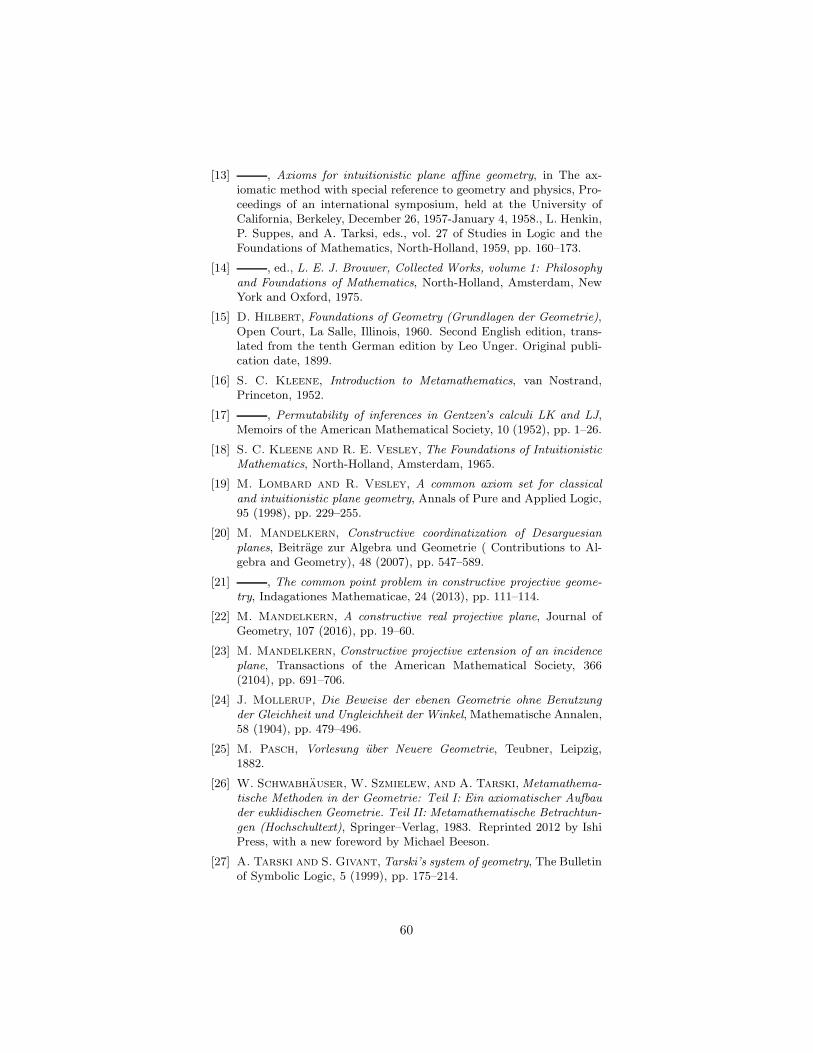
[13] , Axioms for intuitionistic plane affine geometry, in The ax-iomatic method with special reference to geometry and physics, Pro-ceedings of an international symposium, held at the University ofCalifornia, Berkeley, December 26, 1957-January 4, 1958., L. Henkin,P. Suppes, and A. Tarksi, eds., vol. 27 of Studies in Logic and theFoundations of Mathematics, North-Holland, 1959, pp. 160–173.

[14] , ed., L. E. J. Brouwer, Collected Works, volume 1: Philosophyand Foundations of Mathematics, North-Holland, Amsterdam, NewYork and Oxford, 1975.

[15] D. Hilbert, Foundations of Geometry (Grundlagen der Geometrie),Open Court, La Salle, Illinois, 1960. Second English edition, trans-lated from the tenth German edition by Leo Unger. Original publi-cation date, 1899.

[16] S. C. Kleene, Introduction to Metamathematics, van Nostrand,Princeton, 1952.

[17] , Permutability of inferences in Gentzen’s calculi LK and LJ,Memoirs of the American Mathematical Society, 10 (1952), pp. 1–26.

[18] S. C. Kleene and R. E. Vesley, The Foundations of IntuitionisticMathematics, North-Holland, Amsterdam, 1965.

[19] M. Lombard and R. Vesley, A common axiom set for classicaland intuitionistic plane geometry, Annals of Pure and Applied Logic,95 (1998), pp. 229–255.

[20] M. Mandelkern, Constructive coordinatization of Desarguesianplanes, Beitrage zur Algebra und Geometrie ( Contributions to Al-gebra and Geometry), 48 (2007), pp. 547–589.

[21] , The common point problem in constructive projective geome-try, Indagationes Mathematicae, 24 (2013), pp. 111–114.

[22] M. Mandelkern, A constructive real projective plane, Journal ofGeometry, 107 (2016), pp. 19–60.

[23] M. Mandelkern, Constructive projective extension of an incidenceplane, Transactions of the American Mathematical Society, 366(2104), pp. 691–706.

[24] J. Mollerup, Die Beweise der ebenen Geometrie ohne Benutzungder Gleichheit und Ungleichheit der Winkel, Mathematische Annalen,58 (1904), pp. 479–496.

[25] M. Pasch, Vorlesung uber Neuere Geometrie, Teubner, Leipzig,1882.

[26] W. Schwabhauser, W. Szmielew, and A. Tarski, Metamathema-tische Methoden in der Geometrie: Teil I: Ein axiomatischer Aufbauder euklidischen Geometrie. Teil II: Metamathematische Betrachtun-gen (Hochschultext), Springer–Verlag, 1983. Reprinted 2012 by IshiPress, with a new foreword by Michael Beeson.

[27] A. Tarski and S. Givant, Tarski’s system of geometry, The Bulletinof Symbolic Logic, 5 (1999), pp. 175–214.

60

[28] A. Troelstra, Metamathematical Investigation of IntuitionisticArithmetic and Analysis, vol. 344 of Lecture Notes in Mathematics,Springer-Verlag, Berlin Heidelberg New York, 1973.

[29] , Metamathematical Investigation of Intuitionistic Arithmeticand Analysis, no. 344 in Lecture Notes in Mathematics, Springer,Berlin, Heidelberg, New York, 1973.

[30] D. van Dalen, Extension problems in intuitionistic plane projectivegeometry, Indagationes Mathematicae, 25 (1963), pp. 349–383.

[31] , Heyting and intuitionistic geometry, in Mathematical Logic,P. Petrov, ed., Plenum Press, New York, 1990, pp. 19–27.

[32] , “Outside” as a primitive notion in constructive projective ge-ometry, Geom. Dedicata, 60 (1996), pp. 107–111.

[33] G. Veronese, Fondamenti di geometria a piu dimensioni e apiu specie di unita rettilinee esposti in forma elementare. Lezioniper la scuola di magistero in matematica, Padova: Tipografiadel Seminario. Digitized by Cornell University Library. Italiantext available at http://ebooks.library.cornell.edu/cgi/t/text/text-idx?c=math;idno=01460002, 1891.

[34] J. von Plato, The axioms of constructive geometry, Annals of Pureand Applied Logic, (1995), pp. 169–200.

61