Embed Size (px)
Citation preview

Bridging the gap between ecosystem modelling tools
using geographic information systems
Jeroen Gerhard Steenbeek
September 2012
A dissertation submitted in partial fulfilment of the requirements for the degree of
Master of Science in GIS and Environment,
The Manchester Metropolitan University.
Department of Environmental and Geographical Sciences
The Manchester Metropolitan University
Vrije Universiteit, Amsterdam
In collaboration with
The University of British Columbia, Canada

MSc Thesis Jeroen Steenbeek i
Declaration of originality
This is to certify that the work is entirely my own and not of any other person, unless explicitly
acknowledged (including citation of published and unpublished sources). The work has not previously
been submitted in any form to the Manchester Metropolitan University or to any other institution for
assessment for any other purpose.
Signed: Date:

MSc Thesis Jeroen Steenbeek ii
Abstract
The effects of climate change and human interactions on marine ecosystems are felt throughout the
world, yet these effects are still poorly understood. Research efforts to attain understanding are
hampered by the limitations of present-day ecosystem models to address the interrelated dynamics
between climate, ocean chemistry, marine food webs, and human systems due to the discreet sciences
that these models derived from.
This thesis seeks to simplify interdisciplinary model interoperability by separating its various technical
and scientific challenges into a flexible and modular framework using open source GIS technology and
common software development paradigms. A prototype of this framework is used to drive the food web
dynamics of an existing and published marine ecosystem model with two spatial-temporal series of
primary productivity. Results show that the predictive capabilities of the model enhanced by better
reflecting observed species population trends, which is a promising step toward future implementations
of the framework, such as in the ambitious end-to-end Nereus Model (Christensen, 2012).

MSc Thesis Jeroen Steenbeek iii
Acknowledgements
I wish to express my gratitude to a number of people for the realization of this thesis.
First and foremost I wish to thank my supervisors, Dr. Jianquan (James) Cheng at Manchester
Metropolitan University, Jasper Dekkers at UNIGIS Amsterdam, and Villy Christensen at the UBC
Fisheries Centre in Vancouver, Canada. I am particular grateful to Villy Christensen for the opportunity
to implement this thesis as part of my day-to-day work activities; without this opportunity this thesis
would not have existed.
I want to thank Joe Buszowksi for spending many hours involuntarily debugging the spatial framework
while trying to integrate it in the Nereus model, and for his feedback when I was designing the spatial
framework. I want to thank Carl Walters for still being able to make sense of the computations in
Ecospace after all that it has been though, and I wish to thank Daniel Pauly for reviewing the case study.
My deep thanks go to my partner Marta Coll Montón, te quiero mucho, for reviewing this manuscript
many times, for providing the Adriatic model, and for her insights in the biological dynamics expressed
in the case study. I promise that I will not write another thesis. Not right now, at least.
Leigh Gurney, Nicolas Hoepffner and Pascal Derycke at the Joint Research Centre in Italy I wish to thank
for the primary production data for the case study, and the excellent collaboration that followed.
In Barcelona, Spain, Isabel Palomera and the ECOTRANS project enabled me to work at the Instituto de
Ciencias del Mar for several months, which was downright fantastic and productive.
Dan Ames provided valuable help with DotSpatial, and enabled NetCDF file support for this library.
Several people provided the occasional gems of inspiration that kept this thesis moving. Beth Fulton and
Mark Hepburn at CSIRO were never too busy to discuss ideas about integrated ecosystem modelling

MSc Thesis Jeroen Steenbeek iv
approaches. Hassan Monsour at the UBC Department of Mathematics and Computer Science
contributed valuable suggestions for spatial statistics. Dalai Felinto, Kristin Kleisner, Fred Le Manach,
Deng Palomares, and Audrey Valls along with many others at the UBC Fisheries Centre were there with
advice when I needed it. Thank you all.
Lastly, I wish to thank Ethan and Sascha for still thinking that Ecopath rocks, although I yet have to find
out exactly what that means in scientific terms.
This study was conducted through the NF-UBC Nereus Program, a collaborative initiative conducted by
the Nippon Foundation, the University of British Columbia, and five additional partners. The work is a
product of Nereus’ international and interdisciplinary effort towards global sustainable fisheries.

MSc Thesis Jeroen Steenbeek v
Table of contents
1 Introduction .......................................................................................................................................... 1
1.1 Aim and objectives ........................................................................................................................ 3
1.2 Ethical issues ................................................................................................................................. 4
2 Review of relevant literature ................................................................................................................ 5
2.1 The need for marine ecosystem modelling .................................................................................. 5
2.2 A brief overview of GIS ............................................................................................................... 10
2.3 Summary ..................................................................................................................................... 14
3 Material and methods ........................................................................................................................ 17
3.1 Ecological model ......................................................................................................................... 17
3.2 Framework .................................................................................................................................. 21
4 Prototype ............................................................................................................................................ 44
5 Case study ........................................................................................................................................... 51
5.1 Introduction ................................................................................................................................ 51
5.2 Methodology ............................................................................................................................... 52
5.3 Results and discussion ................................................................................................................ 63
5.4 Conclusions of the case study ..................................................................................................... 66

MSc Thesis Jeroen Steenbeek vi
6 General discussion .............................................................................................................................. 68
7 Conclusions and future developments ............................................................................................... 71
8 References .......................................................................................................................................... 74
Annex A Principles of the Ecopath with Ecosim approach .................................................................... 88
Annex B GIS toolkit evaluation ............................................................................................................ 103
Annex C Additional case study results and discussion ........................................................................ 104

MSc Thesis Jeroen Steenbeek vii
List of figures
Figure 1 – Structure of the EwE6 software with plug-ins. ............................................................................ 8
Figure 2 - An overview of published Atlantis, EwE, and OSMOSE models (Adapted from Fulton, 2010). . 16
Figure 3 – The main Ecospace user interface in the EwE6 desktop software.6.3. ..................................... 19
Figure 4 - A spatial temporal data framework that encapsulates the Ecospace model, and provides
access to a wide range of spatially enabled data sources. ......................................................................... 20
Figure 5 - Conceptual overview of the framework, which provides external GIS data to Ecospace model
initialization and at runtime, and provides Ecospace results in spatial data formats when the model
execute. ....................................................................................................................................................... 24
Figure 6 - Conceptual layers of functionality within the framework when integrating external data into
Ecospace: (1) inter-model data exchange to match Ecospace parameterizations, (2) GIS data conversion
to match Ecospace resolution, (3) Ecospace data integration, and (4) post-run analysis. ......................... 25
Figure 7 - Conceptual layers of functionality when the framework dispenses Ecospace data: 2.
conversion of Ecospace results to spatial formats, and (1) inter-model data exchange, and (4) post-run
analysis. ....................................................................................................................................................... 26
Figure 8 – A modular approach to reading GIS data. Different GIS data access modules offer the
framework access to unique GIS data formats and storage media, and modules can be added without
disrupting existing modules. ....................................................................................................................... 27
Figure 9 - Conceptual overview of EwE in a model interoperability framework, featuring a central time
step controller, and brokers between dedicated models that propagate results and feedback effects. .. 29
Figure 10 - A schematic functional design of the framework, displaying how external data is brought into

MSc Thesis Jeroen Steenbeek viii
Ecospace. .................................................................................................................................................... 31
Figure 11 - Data exchange framework – producing data. .......................................................................... 33
Figure 12 - An illustration of how plug-in points are integrated into the flow of the EwE6 application. ... 34
Figure 13 - Interaction diagram, showing how Ecospace, an adapter, a dataset, a converter and a GIS
toolkit communicate to perform the core framework task to read external data. .................................... 36
Figure 14 - The EwE6 user interface, with indications to the presence of the external spatial data
facilities: (1) an item in the EwE navigation tree, (2) a configuration option in the Ecospace menu, (3) an
indicator beside a layer in the Ecospace map interface to indicate each layer connected to external data,
and (4) an indicator to notify the user of the number of active external data connections. ..................... 45
Figure 15 - The central interface to manage external data connections to the Ecospace map, showing (1)
Ecospace layers that accept external data connections, (2) elements to manage data sets, and (3)
elements to select and configure converters. ............................................................................................ 46
Figure 16 - User interface, developed for this thesis, for configuring a data set to a series of spatial-
temporal files. A dataset needs a description (1). Files can be added from folders (2). Every file is tagged
by date (3), which allows the spatial-temporal framework to locate external data when Ecospace
executes. The dataset in this figure is connected to a directory of netCDF files........................................ 48
Figure 17 – The EwE6 user interface that provides a cursory overview of the spatial and temporal
compatibility of external data with an Ecospace model. The map section (1) of the interface shows the
area of the Ecospace map (2), and provides details for selected data connection and time step (3). ...... 49
Figure 18 – EwE6 interface from where the Ecospace model is executed. The status panel (1) shows an
excerpt from the spatial operations log as produced by the spatial temporal data framework. .............. 50
Figure 19 - The Northern-Central (NC) Adriatic Sea study area. The light-grey area represents the spatial
MSc Thesis Jeroen Steenbeek ix
coverage of the ecological model available. Current protected areas and biological conservation zones
are also indicated. ....................................................................................................................................... 53
Figure 20 - Ecospace study map of the Northern-Central Adriatic Sea. This map with a reference image
illustrates the spatial fit in the Ecospace maps interface. .......................................................................... 56
Figure 21 –Minimum, maximum, and mean primary production rates for the North-Central Adriatic in
the monthly dataset. ................................................................................................................................... 57
Figure 22 - Minimum, maximum, and mean primary production rates for the North-Central Adriatic in
the annual dataset. ..................................................................................................................................... 57
Figure 23 – A conceptual overview of how the spatial-temporal data framework loads, adjusts, and
integrates spatial data into Ecospace. ........................................................................................................ 58
Figure 24 – The new user interface, developed for this MSc thesis, to connect sets of external spatial-
temporal data to Ecospace layers. .............................................................................................................. 60
Figure 25 – Flow of GIS data through the spatial-temporal data framework for this case study. GIS data
files are located and loaded, converted to suitable raster data consumption by Ecospace, and then
rescaled and copied into the internal Ecospace data layers. ..................................................................... 60
Figure 26 - Original relative primary production map in the Ecospace model. .......................................... 61
Figure 27 - External data connection to the original primary production distribution map of Figure 26. . 61
Figure 28 – Minimum, maximum, and mean values for the monthly and annual primary production
datasets, extracted by the spatial framework for relevant Ecospace cells. ............................................... 63
Figure 29 – Predicted relative (final / initial value) biomass of phytoplankton for each of the scenario
runs. The start of SeaWIFS data being read by the modelling framework is indicated by a black vertical
line............................................................................................................................................................... 64

MSc Thesis Jeroen Steenbeek x
Figure 30 - Original dataset distributions of primary production for 2007: (a) December 2007, (b) annual
average for 2007. ........................................................................................................................................ 65
Figure 31 - Ecospace map showing the distribution of relative biomass of phytoplankton for the last year
of the simulation, 2007. Results are related with the model (a) without external PP data, (b) with
monthly PP data, and (c) with annual PP data. ........................................................................................... 66
Figure 32 - The habitat capacity model as a modular model. Users can opt to (a) compute capacity from
environmental driver layers, (b) compute capacity from habitats, or (c) bypass options (a) and (b), and
directly derive habitat capacity from external species envelope models. Options (a) and (b) can be
employed in conjunction. Data for (a), (b) and (c) can be either manually entered, or can be driven by
the framework. ........................................................................................................................................... 69

MSc Thesis Jeroen Steenbeek xi
List of acronyms
E2E (model) End to End model
ESRI Environmental Sciences Research Institute
EwE6 Ecopath with Ecosim version 6
FOSS Free and Open Source Software
GFCM General Fisheries Commission for the Mediterranean
GIS Geographic Information System
GMIS Global Marine Information System
GRASS Geographic Resources Analysis Support System
JRC Joint Research Centre
MEM Marine ecosystem model
MIMES Multiscale Integrated Model of Ecosystem Services
netCDF Network Common Data Form
NOAA National Oceanic and Atmospheric Administration
UBC University of British Columbia
MSc Thesis Jeroen Steenbeek 1
“An animal that is very abundant, before it gets extinct it
becomes rare. So you don't lose abundant animals. You
always lose rare animals. Therefore, they're not perceived as
a big loss.”
- Daniel Pauly (2010)
1 Introduction
The effects of climate change and human interactions on marine ecosystems are felt throughout the
world, yet these effects are still poorly understood. Environmental changes and human interactions
have profound and often irreversible impacts on marine and terrestrial ecosystems. Globally, realization
is dawning that all environmental processes are interconnected, that terrestrial ecosystems cannot exist
without healthy, productive oceans, and that past approaches to manage ecosystems have been
insufficient to stop many aspects of our environment from steadily declining.
Marine ecosystem models (MEM) are mathematical tools that help analyze and forecast dynamics
within marine ecosystems, and how these ecosystems respond to external stressors such as fishing and
changes in environmental factors. MEM tools yield vital information for policy makers and scientists
alike to address issues such as sustainable fishing, marine conservation, and long-term food security.
However, the majority of present day MEM tools were originally built as expert tools by and for
scientists to address questions of a specific scope, and thus have limited applicability. Based on largely
proprietary data formats and coding platforms, existing MEM tools are often physically unfit to
collaborate with other modelling approaches to address matters beyond the scientific discipline that
models were written for. Yet, changing climate conditions require unprecedented analytical capabilities
that address the interrelated dynamics between climate, ocean biochemistry, marine organisms, and

MSc Thesis Jeroen Steenbeek 2
socio-economic systems, crossing several traditional scientific disciplines in the process and covering
geographical and temporal scales of several orders of magnitude. MEM tools need to become flexible
enough to collaborate with other models in order to put their expert capabilities to use in such a large,
analytical context.
Coupling the science of discrete MEM tools requires significant interdisciplinary effort. This challenge is
exuberated by lack of communication protocols and common data standards between modelling
approaches. Geographic Information Systems offer essential data formats and operations that provide
the foundation for implementing the link between models, while industry-standard software design
practices offer the necessary structures to enable models to collaborate. Drawing on all three disciplines
this thesis proposes a flexible framework for bridging the gap between MEM tools using GIS.

MSc Thesis Jeroen Steenbeek 3
1.1 Aim and objectives
The final aim of this thesis is to ascertain and improve the feasibility of MEM tools to interoperate via
GIS data standards by examination of marine ecosystem modelling needs, available models and tools,
interoperability criteria, data standards used in the scientific community, and scientific issues that arise
from current limited model interoperability.
This thesis puts forth a technical framework that allows traditional ecosystem models to provide and
consume geospatial data in a generic matter, using generic data formats and communication protocols,
as a foundation for scientific collaboration to address questions beyond the scope of a single model. The
aim is to fill a void in the discussion of model interoperability by providing set of technical conventions
onto which environmental model interoperability can be constructed.
The thesis aim is achieved by:
• Reviewing relevant literature, focusing on prominent marine environmental models and marine
ecosystem models (MEM) tools, model interoperability needs and strategies, and existing and
foreseen environmental modelling interoperability standards;
• Examining the modelling capabilities, data needs, and GIS capabilities of the most widely used
MEM tool, Ecopath with Ecosim version 6 (EwE6), for modelling climate change;
• Researching, testing, and analyzing the scientific challenges that derive from using GIS tools to
connect EwE6 to spatial-temporal primary production data;
• Developing a prototype interoperability framework, and testing this framework with a spatio-
temporal time series to drive the base of a food web in EwE6 using an existing, published
ecosystem model;

MSc Thesis Jeroen Steenbeek 4
• Developing a prototype data delivery framework for EwE6 to provide its model results in any GIS
format suitable for interoperability with other models and spatial frameworks.
1.2 Ethical issues
Agreements to use the data for this thesis have been established through the University of British
Columbia (Vancouver, Canada), and its cooperation with the Institute of Marine Sciences (Barcelona,
Spain) and the Joint Research Center (Ispra, Italy) of the European Union.
Agreements to use the Ecopath models for this thesis have been established through the University of
British Columbia, the Ecopath Research and Development Consortium, and the principle investigator
behind the EwE6 model approach, Dr. Villy Christensen.

MSc Thesis Jeroen Steenbeek 5
“I believe, then, that the cod fishery, the herring fishery, the
pilchard fishery, the mackerel fishery, and probably all the
great sea fisheries, are inexhaustible; that is to say, that
nothing we do seriously affects the number of the fish. And
any attempt to regulate these fisheries seems consequently,
from the nature of the case, to be useless.”
- Thomas Huxley (1883)
2 Review of relevant literature
2.1 The need for marine ecosystem modelling
The understanding of the marine environment has increased dramatically in the past few decades
(Fulton, 2010), and Marine Ecosystem Models (MEM) have become indispensable tools for ecosystem-
based management purposes (e.g., Leslie and McLeod, 2007; Espinosa-Romero et al., 2011). However,
understanding of the cumulative impacts of a rapidly changing climate (e.g., Diaz and Markgraf, 2000;
Orr et al., 2005; Hansen et al., 2006; Stock et al., 2011) and anthropogenic interactions (e.g., Hilborn
and Walters, 1992; Pauly et al., 1998), and what these individual impacts mean for an ecosystem as a
whole, is still in a budding stage (Ainsworth et al., 2011; Coll et al., 2012).
A growing body of research suggests that changes in the atmosphere have far reaching consequences
for the oceans, such as unequal shifts of marine species distribution ranges (Stock et al., 2011) in
response to changing ocean temperatures (Hansen et al., 2006), increasing anoxic water conditions due
to the formation and die-off of plankton blooms (Stock et al., 2011), decreased ability of corals,
crustaceans, and molluscs to build shells and exoskeletons due to ocean acidification (Orr et al., 2005;

MSc Thesis Jeroen Steenbeek 6
Fabry et al., 2008), and the projected increase in frequency of major climatological events such as ‘El
Niño’ (Diaz and Markgraf, 2000; Emanuel, 2005; Edgar et al., 2010) that have the capability to disrupt
global weather patterns (Jacobs et al., 1994; Diaz and Markgraf, 2000; Webster et al., 2005), impacting
the functioning of ecosystems and human ecosystems for several years.
2.1.1 End-to-end modelling
In a response to understand these far-reaching but interrelated effects a new type of ecosystem model,
the end-to-end (E2E) model, has emerged. E2E models differ from traditional models by extending their
scope to include the components of, and dynamics between, climate change, biochemical
oceanographic processes, marine food webs models, and the human systems that interact with the
marine environment (Fulton, 2010; Rose et al., 2010).
The idea of E2E modeling is receiving significant scientific interest in peer-reviewed literature (e.g.,
Travers et al., 2007; Erturk et al., 2008; Libralato and Solidoro, 2009; Rose et al., 2010; Steele and
Ruzicka, 2011), but only two ecosystem models, Atlantis and InVitro approaches (Fulton et al., 2004;
Gray et al., 2006; Fulton, 2010), truly consider the interrelated end-to-end dynamics. Other modelling
approaches show significant promise by encapsulating new dynamics as they evolve such as OSMOSE
(Shin and Cury, 2001; Shin et al., 2010), MIMES (Boumans and Costanza, 2007), NEMURO.FISH (Kishi et
al., 2007) and EwE6 (Christensen and Walters, 2004; Christensen and Lai, 2007).
Recent inventories by Plaganí (2007), Travers et al. (2007) and Fulton (2010) describe the challenges
that are faced by E2E models. For example, they need to:
• Include processes that are traditionally contained within discrete scientific disciplines, and
implement bi-directional transfer of appropriate information between different sciences to
reflect feedback effects between ecosystem components;

MSc Thesis Jeroen Steenbeek 7
• Join processes that typically operate on spatial and temporal scales that may differ by several
orders of magnitude;
• Include a potentially open-ended number of species, chemicals, socio-economic aspects, each
described in a proprietary manner using different and potentially incompatible units;
• Assess the impacts and cascading effects of anthropogenic perturbations in every aspect of
marine ecosystems;
• Assess and communicate the impacts of uncertainty.
Prevalent marine ecosystem modelling approaches such as Atlantis, NEMURO.FISH and Osmose address
these challenges by integrating more dedicated functionality of ever increasing scope within their
proprietary frameworks and code environment. Therefore, the resulting E2E models are inflexible
complexes that require extensive funding and expertise to parameterize and operate. Moreover, the
fixed connections within the E2E imply a fixed scientific pathway through the modelling complex, which
does not allow for testing of different hypothesis within the E2E by switching model components.
More modular modelling frameworks, such as the Multiscale Integrated Model of Ecosystem Services
(MIMES), offer an extensible set of modules that collaborate on a common set of data definitions and
conventions focused on ecosystem value (Boumans and Costanza, 2007; Nelson and Daily, 2010).
Although providing a wide range of advanced capabilities to represent the socio-economic aspects of
end-to-end models, the value-focused view of this model offers limited consideration of marine
ecosystems beyond exploited marine species, and is in particular unsuitable to represent ecology and
the effects of climate change (Waage et al., 2008; Nelson and Daily, 2010).

MSc Thesis Jeroen Steenbeek 8
Lastly, version 6 of the Ecopath with Ecosim food web model (EwE6) takes a different approach, and was
designed with model interoperability in mind. EwE6 is an open source product, which enables
development of linkages to other models with reasonable ease. With model interoperability in mind a
plug-in system was built into the very design of the EwE6 software, which enables users to extend the
capabilities of the software without having to alter the source code of the approach (Christensen and
Lai, 2007). The EwE6 software will be further discussed in section 3.1 and more detail can be found in
Annex A.
2.1.2 Caveats to end-to-end modelling
There is no single ideal model to address any aspect of reality because every model is based on
embedded hypothesis and assumptions (e.g., Christensen and Walters, 2005; Fennel, 2008; Shin et al.,
2010). Models are built for purposes and thus have unique predictive capabilities, strengths and
weaknesses. Therefore, to validate predictions and quantify uncertainty, it is generally agreed that
important scientific questions should be scrutinized with as many model as possible (e.g., Fulton, 2010).
This paradigm has not yet been applied to E2E models, which are exceptionally sensitive to uncertainty
propagation due to their complexity, many data conversions, and long computational paths (Travers et
Figure 1 – Structure of the EwE6 software with plug-ins.

MSc Thesis Jeroen Steenbeek 9
al., 2007; Rose, 2012).
Integrating MEM tools toward an end-to-end model requires unprecedented scientific and technological
effort (Fulton et al., 2009; Gallagher et al., 2010; Rose et al., 2010), but other than Fulton’s InVitro (Gray
et al., 2006), no practical implementations of technological frameworks for model interoperability have
surfaced in the literature. Theoretical paradigms abound detailing diverse approaches to connect lower
and higher trophic models (e.g., Argent, 2004; Rose, 2012), but without exception these theories are
posed without practical guidelines toward implementation, and without any consideration toward
standardization of model interoperability or model collaboration to facilitate flexibility in end-to-end
model construction.

MSc Thesis Jeroen Steenbeek 10
2.2 A brief overview of GIS
2.2.1 GIS and modelling
Geographic Information Systems have been an indispensable component of environmental modelling
(e.g., Goodchild et al., 1993; Wesseling et al., 1996; Jolma et al., 2008). Present-day marine
environmental models are interdisciplinary efforts that depend on the spatial context provided by GIS to
be successful: specialist models derive ecological, environmental, and socio-economic indicators - simple
measures that represent key components of the modelled system with a meaning beyond the attributes
that are directly measured – which only by means of GIS functionality are placed within a specific
geographic context. Mapping the environmental variability of indicators across a geographic area
enables an integrated assessment of individual, location-bound indicators within a broader geographic
context (Wesseling et al., 1996).
GIS was conceived for terrestrial applications, which are characterized by largely discrete boundaries,
are highly suitable for representation in a GIS, and can be geo-processed with relative simple two-
dimensional GIS operations such as overlaying, buffering, reclassification and Boolean operators with
high accuracy (Wesseling et al., 1996; Valavanis, 2002; Levin et al., 2009). When GIS migrated to the
marine realm in the late 1980s and early 1990s the technology was faced with an entirely new set of
challenges. The underwater environment is highly heterogeneous, dynamic, inter-mixed, and three-
dimensional with unclear boundaries. Dynamic marine processes such as upwelling, gyres, and
advection require consideration of the vertical dimension and time, at scales that differ in several orders
of magnitude (e.g., Valavanis, 2002; Levin et al., 2009). Representing and analysing marine entities such
as species, nutrients, oxygen, and pollutants, which disperse and interact in ways that cannot be
explained using mere geographic location and proximity, requires additional knowledge of several

MSc Thesis Jeroen Steenbeek 11
marine disciplines such as biological and physical oceanography, marine biology, and remote sensing.
Marine environmental modelling is an interdisciplinary effort that often relies on integrated
assessments of specialist model tools. Some aspects of marine modelling may be addressed using native
GIS capabilities, such as habitat classification, watershed modelling, interpretation and classification of
remote sensing imagery, or species distribution mapping. However, addressing the dynamics in a marine
ecosystem often demands integration of GIS and dedicated models to analyze environmental,
biochemical, and biological interactions in a spatial context including mechanistic approaches using
modelling capabilities.
2.2.2 Challenges to integrating GIS and ecosystem modelling
The integration of the different ecosystem components into spatial analysis poses a series of challenges
that are reviewed below:
Scales
In marine ecology, it is a well-established fact that individual components of an ecosystem are best
modelled at relevant scales (Levin, 1992; Shin and Cury, 2001; Solimini et al., 2009). However, the
adequate spatial and temporal scale to model marine phenomena of interest is a daunting task to which
no standard solutions apply (Rose et al., 2010):
• Coarser scales will decrease local variability in data patterns, hence possibly eradicating crucial
interactions that may drive an ecosystem;
• Too fine scales on the other hand may cause phenomena or processes to become over-
represented, introducing computational instabilities and oscillations that approximate
interactions at unrealistic time scales and spatial resolutions (Walters et al., 1999).

MSc Thesis Jeroen Steenbeek 12
Each category of environmental models scrutinizes only directly interacting components at resolutions
of space, time and modelled entities relevant to that model (Levin, 1992). Meaningful translation of data
between two models is a task to which GIS environments provide only limited facilities.
Metadata standards
Lack of semantic data standards poses the greatest challenge to enable the various components of
spatial data infrastructures. This problem is exacerbated when attempting to unify ecosystem models in
GIS environments since the field of ecosystem modelling suffers from a similar lack of commonly
adopted standards (Rose, 2012).
The need for semantic data standards for ecology has been long acknowledged for ecological
interoperability in spatial and non-spatial systems (e.g., Michener et al., 1997), and several efforts aim to
address this. Freely accessible taxonomic repositories such as FishBase (Froese and Pauly, 2010), the
Ocean Biogeographic Information System (Grassle, 2000) and the World Register of Marine Species
(WoRMS; Appeltans et al., 2011) are ongoing efforts to bring a measure of order in the surprisingly
turbulent field of species classifications. Other approaches aim to centralize storage and distribution of
ecological data in repositories such as Dryad (Scherle et al., 2008), an effort that requires metadata
standards with ecological and GIS components (Greenberg et al., 2009). Separately, the text-based
Ecological Metadata Language (EML) shows promise as a flexible structure for describing ecological data,
its purpose and applicability in spatial and non-spatial contexts (e.g., Michener, 2006; Gil et al., 2008;
Whitlock, 2011).
However, adaption of standards by higher-trophic ecosystem models is in its infancy. There are no
binding rules and best practices how to construct higher-trophic models, which species to include, which
species to aggregate, and at what spatial and temporal scales to assess species dynamics (e.g., Rose et
MSc Thesis Jeroen Steenbeek 13
al., 2010). Ecosystem models are inherently constructed with different motivations to address unique
questions, requiring different levels of detail and different collections of variables (Fegraus et al., 2005).
Uncertainty
Uncertainty is a key threat to the liability of numerical models. Jager and King (2004) summarize the
classical sources of uncertainty in ecological models as (i) uncertainty in measurements; (ii) cartographic
uncertainty; (iii) uncertainty error propagation and amplification through model computations; and (iv)
uncertainty between alternate input data sets. Francis et al. (2011) add a new source of uncertainty as
the limited experience with predicting the behaviours of external, anthropogenic drivers: human
systems are immensely complex, and future trends in urbanization, land use and economic
developments will inevitably affect ecosystems in yet poorly understood ways.
Uncertainty and error propagation in GIS have received considerable attention since the early days of
GIS, where the complexity of geospatial operations amplify error due to data accuracy, quality, and error
(e.g., Heuvelink, 1998; Crosetto and Tarantola, 2001). Ecological models are subject to various types of
uncertainty and error propagation (e.g., Hilborn and Walters, 1992; Heuvelink, 1998; Crosetto et al.,
2000; Jager and King, 2004; Rose et al., 2010). The effect of error are exacerbated when environmental
models and GIS are used in conjunction (Crosetto and Tarantola, 2001; Couclelis, 2003; Kacprzyk, 2010).
In inter-model scenarios, feedback effects amplify error further, and thus subtle parameter variations
due to uncertainty may lead to significant changes in long-term predictions (Kearney et al., 2012). In a
complex modelling approach, error needs to be measurable. It is necessary to assess how uncertainty in
input data, model parameters, etc. propagates through individual model components, but also through
the individual linkages between the models in an integrated assembly. Furthermore, measures of fit of
intermediate model results to observed data may provide further diagnostics on model uncertainty.

MSc Thesis Jeroen Steenbeek 14
2.3 Summary
The effects of climate change have underpinned the already known fact that all ecosystems are related,
and that ecosystem modelling tools to date are insufficient to perform an integrated assessment of
dynamics in the entire ecosystem at long term, large spatial scales. In order to assess global impacts of
climate change and to make predictions about the future of our oceans, integrated analysis will have to
be performed at global scales. For managing global issues involving climate and sustainable utilization of
the marine environment we will first require global understanding of these issues, for which the
modelling capacity is slowly emerging.
A major challenge for ecosystem modellers that is still waiting is to build modelling capacity on an
integrated, global scale. Currently a wide array of modelling approaches exist that support in-depth
exploration of specific aspects of the environment, but models are rarely linked, operate on different
scales in time and space and under not necessarily related assumptions. These models were not
engineered to interoperate, lacking features to exchange data with other models in a standardized
manner. Integrated modelling frameworks on the other hand are built to address overarching questions,
but are in turn criticized for not being able to cover phenomena at proper level of detail.
GIS technology forms an essential part of environmental modelling, but GIS capabilities are underutilized
due to a lack of semantic data standards within the realm of GIS itself, and lack of ecological data
standards in marine ecology. The lack of generic abilities to communicate hampers efforts to leverage
the full capabilities of GIS and ecological models for inter-model assessments, and yields hybrid
approaches that are characterized by either a partial implementation of GIS functionality into ecosystem
models, or by a partial implementation of ecological assessments within a GIS (e.g., Valavanis, 2002;
Manso and Wachowicz, 2009). As a result, such end-to-end models are developed as narrow paths,

MSc Thesis Jeroen Steenbeek 15
based on inflexible chains of interwoven models, lacking transparency to validate embedded hypothesis.
To advance on our understanding of ecosystem dynamics and our capability to forecast, science and
technology cannot be viewed separately and should be scrutinized in equal measure as we push
forward, while we take in the important lessons from past research. This applies well to the context of
E2E modelling. There is large potential that the 1990s struggles of merging MEM tools into more capable
marine modelling approaches will be repeated all over again when constructing state-of-the-art E2E
models. End-to-end models are staggering efforts that aim to address atmospheric, physical, biological,
and socio-economic factors across wide spatial and temporal scales, crossing many traditional scientific,
technical, and political boundaries. Such endeavours cannot be accomplished by scientific experts alone,
but should draw benefit in equal measure from lessons learned in technical and social sciences.
It would, for instance, be very exciting if we could reuse the existing, published higher trophic level
models in Figure 2 for addressing larger ecosystem questions by simply re-engineering those tools to
better collaborate for this larger scope without having to rebuild new models. This thesis hopes to set
first steps toward this standardization.
This thesis puts forth a technical framework that allows traditional ecosystem models to provide and
consume Geospatial data in a generic matter, using generic data formats and communication protocols.
This provides a foundation for scientific collaboration to address questions beyond the scope of a single
model. The thesis may advance in filling a void in this discussion by providing the theorists and scientists
with a set of technical conventions onto which MEM model interoperability can be constructed.

MSc Thesis Jeroen Steenbeek 16
Figure 2 - An overview of published Atlantis, EwE, and OSMOSE models (Adapted from Fulton, 2010).
MSc Thesis Jeroen Steenbeek 17
“Make things as simple as possible, but not simpler”
- Albert Einstein
3 Material and methods
3.1 Ecological model
For this thesis the ecological modelling approach Ecopath with Ecosim version 6 or EwE6 has been
selected to serve as a test case for spatial-temporal model interoperability. EwE is the most widely used
model for assessing aquatic food web dynamics and the impact of human exploitation (Figure 2), with an
estimated 6000 users in more than 150 countries, and with more than 600 academic publications to
date (ProQuest, 2012). EwE is increasingly used in ecosystem based management assessments (e.g.,
Christensen and Walters, 2005, 2011; Cisneros-Montemayor et al., 2012), despite criticism for its
perceived simplicity (Plaganyí, 2007).
The software is developed using the Microsoft .NET platform (Christensen and Lai, 2007), which offers a
range of technical benefits such as compatibility with a suite of programming languages and the
theoretical ability to run on any operation system (ECMA International, 2012).
The EwE6 approach is deemed as prime candidate for model interoperability. The software has seen a
wide range of applications and is increasingly used in ecosystem based management assessments (e.g.,
Christensen and Walters, 2005, 2011; Cisneros-Montemayor et al., 2012). The need for integrated
ecosystem assessments have led to recent additions to the approach, such as for example a
management strategy evaluation module, an integrated species distribution envelope model, and
facilities to integrate with digital taxonomic libraries. Migration to the .NET environment facilitated the
MSc Thesis Jeroen Steenbeek 18
additions of a plug-in system that allows users to complement the EwE6 approach with new
functionality without making physical changes to the EwE source code. As part of this thesis, the
software is being extended via plug-ins to interoperate with external spatial-temporal models.
Annex A provides a cursory overview of EwE version 6.2.0 (released 20 June 2011) to illustrate its
potential in a model interoperability environment. The core model of the EwE approach is the Ecopath
model (Christensen and Pauly, 1993; Pauly et al., 2000; Christensen and Walters, 2004), a static model of
marine ecosystems. NOAA, the National Oceanic and Atmospheric Administration, celebrated the
approach as one of the ten biggest scientific breakthroughs in its 200 year existence (NOAA, 2007). Most
relevant to this thesis, though, is that the static mass-balance snapshot model Ecopath became the
precursor to the time-dynamic model Ecosim (Walters et al., 1997; Walters, 2000) and the time-space
dynamic model Ecospace (Walters et al., 1999, 2010).
In 1995 the Ecosim module was added to the desktop software for exploring past and future impacts of
fishing and environmental disturbances over time. Ecosim re-expresses the linear Ecopath equations as
a set of differential equations and solves these for regular time intervals for any given time period,
under the assumption that biomasses and the ability of any group to produce and consume are variable.
The third core module of EwE is the spatial/temporal model Ecospace, a spatially explicit multi-species
ecosystem model (Walters et al., 1999, 2010; Christensen et al., 2003; Christensen and Maclean, 2011).
Ecospace has been widely applied to quantify the spatial impacts on marine species due to fishing, and
to analyse the outcomes of management options such as the establishment of marine protected areas
and its impact in terms of spatial distribution of marine species and fishing effort (e.g., Walters, 2000;
Martell et al., 2005; Walters et al., 2010; Fouzai et al., 2012). It can also be used to develop spatial
optimization routines (Christensen et al., 2009) and assess the impact of climate change by linking the

MSc Thesis Jeroen Steenbeek 19
Ecospace model with low trophic level models (Fulton, 2011).
The Ecospace model was built to model biomass interactions within an ecosystem across a two-
dimensional grid over time. Ecospace distributes Ecopath biomass values of functional groups across a
grid of equally sized cells, and uses the Ecosim equations to model how biomasses vary within each cell
in the grid over time by taking trophic interactions, fishing and species movement into account. Spatial
variations in driver variables such as the primary productivity map have significant impacts on the
Ecospace dynamics (Martell et al., 2002).
However, up to version 6.2.0 of the EwE software, a continued and major shortcoming of the Ecospace
routines has been its lack of facilities to read and produce true geo-spatial data into driver layers. Map
data to Ecospace needs to be sketched onto the map user interface (Figure 3) by hand using a mouse, or
can at most be read carefully crafted comma-separated text files without explicit spatial reference.
Facilities that tried to mitigate this lack of functionality, existent in the precursor to EwE6, were not
Figure 3 – The main Ecospace user interface in the EwE6 desktop software.6.3.

MSc Thesis Jeroen Steenbeek 20
implemented in the EwE version 6 because of limited applicability (Christensen and Lai, 2007).
This thesis addresses the inability of Ecospace to handle GIS data and interact with other spatially
enabled ecosystem models by defining a spatial temporal data framework that encapsulates the
Ecospace model (Figure 4) to interact with a wide range of spatial data sources.
Figure 4 - A spatial temporal data framework that encapsulates the
Ecospace model, and provides access to a wide range of spatially enabled
data sources.
MSc Thesis Jeroen Steenbeek 21
3.2 Framework
The Ecopath and Ecosim models have been successfully linked to other models, but the spatial model
Ecospace has seen little use in this regard due to lack of facilities to exchange data. Since its initial
development in 1999 the ability for Ecospace to exchange spatial-temporal data has been desired.
Continued popularity of the EwE approach, increasing demand for the ability to use the Ecospace model
in conjunction with spatial analytical tools, specialist models, and planning tools such as Marxan (e.g.,
Loos, 2011), and facilities offered by the mature .NET programming environment, gave rise to the idea
of a flexible spatial-temporal data framework to solve the data connectivity shortcomings of Ecospace.
In this chapter such a framework is conceptualized, designed and implemented. First, a theoretical
framework is designed. Requirements for the framework are identified, and a theoretical design for the
framework is discussed. This theoretical framework is then converted to a functional design. Then,
candidate GIS programming toolkits are evaluated and a GIS programming toolkit is selected to
implement a prototype of the framework. Lastly, this prototype is presented.
The terms spatial temporal data framework, spatial framework, or framework may be used
interchangeably for the same principle.
3.2.1 Methodological design
Requirements
From an Ecospace operational perspective, the framework needs to fulfill the following technical
requirements:
1. Provide access to static spatial files of relevant data to generate an Ecospace basemap;

MSc Thesis Jeroen Steenbeek 22
2. Deliver spatial time series of relevant data into Ecospace during execution time to drive the
model;
3. Enable Ecospace to deliver its results as spatial time series for consumption by tools and models
outside of the Ecospace model;
4. Enable read and write access to geospatial data formats and data delivery media common to
the environmental sciences;
5. Enable Ecospace data interoperability for any spatial extent and Ecospace raster cell size.
To serve in an end-to-end model interoperability environment the framework needs to facilitate
Ecospace to:
6. Support bi-directional exchange of spatial-temporal data with an open-ended range of
collaborating models in an end-to-end approach;
7. Support scientifically sound translation of data between external models and Ecospace;
8. Support flexible access to sub-models in the Ecospace model to test different hypothesis;
9. Support the use and exchange of ecological metadata;
10. Store intermediate results to allow assessments of error;
11. Enable outside control to when Ecospace executes a time step.
To serve in a GIS interoperability environment a framework needs to enable Ecospace to:
12. Support for the use and exchange of spatial metadata;
13. Support a suite of geospatial operations needed to interpolate geospatial data into Ecospace;

MSc Thesis Jeroen Steenbeek 23
14. Support a detailed overview of performed data conversions;
15. Provide access to all intermediate data produced to facilitate uncertainty analysis.
Functionally, the framework will be operated by users that may have limited GIS experience. From a
usability point of view, the following additional requirements were identified:
16. Minimize the need for users to interact with the framework without violating framework
capabilities and functionality;
17. Minimize complexity in user interfaces;
Lastly, the framework should not pose any limitations to future unforeseen uses, thus it should:
18. Permit inclusion of access to new file formats, new data delivery media, and new spatial
operations in the future.
Conceptual design
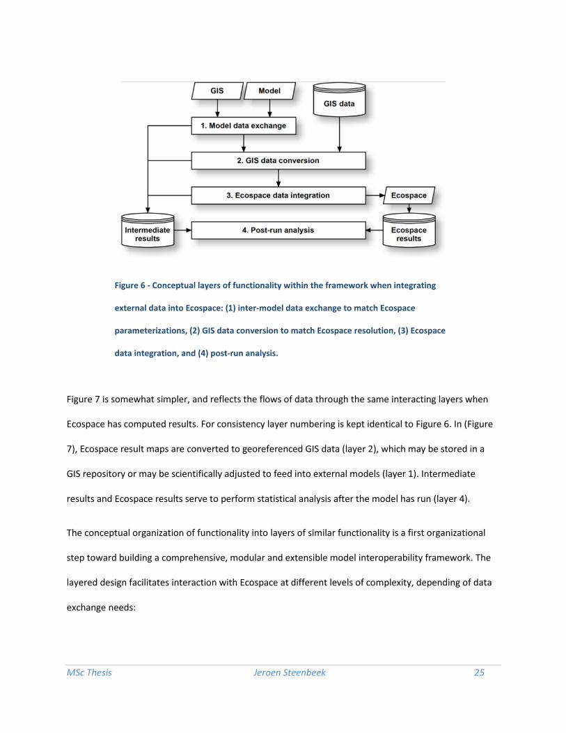
The conceptual integration of the spatial framework into EwE6 is summarized in Figure 5. Spatial data is
either used to define an Ecospace base map at model initialization, or is used to drive Ecospace maps
during every time step. Ecospace results are presented as GIS data through the spatial framework. The
requirements listed in the previous section can be conceptually grouped into layers of functionality
within the spatial temporal data framework, as displayed in Figures 6 and 7.

MSc Thesis Jeroen Steenbeek 24
Figure 6 reflects the flows of data through interacting layers of functionality when external data is
brought into the Ecospace model. Data, derived from external GIS or models, is scientifically adjusted to
fit the parameterization of the Ecospace model (layer 1). The resulting data, or data directly derived
from readily available GIS data sources, is converted to the spatial dimensions of an Ecospace basemap
(layer 2). This data is then inserted in the running instance of the Ecospace model (layer 3). All layers
produce intermediate results, which then, in conjunction with produced Ecospace results, can be used in
statistically analysis for uncertainty.
Figure 5 - Conceptual overview of the framework, which provides external GIS data
to Ecospace model initialization and at runtime, and provides Ecospace results in
spatial data formats when the model execute.
MSc Thesis Jeroen Steenbeek 25
Figure 7 is somewhat simpler, and reflects the flows of data through the same interacting layers when
Ecospace has computed results. For consistency layer numbering is kept identical to Figure 6. In (Figure
7), Ecospace result maps are converted to georeferenced GIS data (layer 2), which may be stored in a
GIS repository or may be scientifically adjusted to feed into external models (layer 1). Intermediate
results and Ecospace results serve to perform statistical analysis after the model has run (layer 4).
The conceptual organization of functionality into layers of similar functionality is a first organizational
step toward building a comprehensive, modular and extensible model interoperability framework. The
layered design facilitates interaction with Ecospace at different levels of complexity, depending of data
exchange needs:
Figure 6 - Conceptual layers of functionality within the framework when integrating
external data into Ecospace: (1) inter-model data exchange to match Ecospace
parameterizations, (2) GIS data conversion to match Ecospace resolution, (3) Ecospace
data integration, and (4) post-run analysis.

MSc Thesis Jeroen Steenbeek 26
Figure 7 - Conceptual layers of functionality when the framework dispenses Ecospace data: 2.
conversion of Ecospace results to spatial formats, and (1) inter-model data exchange, and (4)
post-run analysis.
• Data that is readily available for integration into Ecospace, such as produced by plug-ins that
perform secondary analysis on Ecospace data, can be directly integrated into the running
Ecospace model via layer 3 in Figure 6. GIS processing and model exchange steps can be
bypassed;
• Spatial data that reside outside the EwE6 application but that are scientifically compatible with
spatial driver variables in Ecospace require conversion from external spatial formats to grids that
are compatible with Ecospace. These data enter the framework in layer 2 (see Figure 6), are
loaded and processed by the conversion layer, and then passed on to the integration layer (layer
3 in Figure 6) for further processing;
• Spatial data that cannot be accepted or accessed by Ecospace in their current form will require
scientific translation in layer 1 (see Figure 6), before undergoing conversion to an Ecospace
format in layer 2 and integration in layer 3. Such data may be delivered by external models in a

MSc Thesis Jeroen Steenbeek 27
model interoperability environment, or may reside in a GIS that is able to communicate with the
spatial framework.
Modular organization
Within each layer, facilities must to be available to fulfill the framework requirements earlier identified
in this section. Most of these requirements are deliberately open-ended to offer the ability to cater to
future, unpredictable needs of the framework. Hence, capabilities of the spatial framework should be
allowed to grow when needed. This calls for a modular design of the framework.
Modularity, in software technical terms, is a technique that breaks down functionality in separate,
interchangeable components called modules. A modular program consists of chains of modules that
work together to implement the purpose of a program. Modules can be grouped in similar functionality,
where each module of the same type implements similar functionality in a different way, and modules
of the same type can be freely exchanged to switch functionality without disrupting the flow of a
Figure 8 – A modular approach to reading GIS data. Different GIS data access
modules offer the framework access to unique GIS data formats and storage media,
and modules can be added without disrupting existing modules.

MSc Thesis Jeroen Steenbeek 28
program. Additionally, modules can be added to a program without compromising the workings of the
system (e.g., Cook, 1991; Gamma et al., 1994).
A modular approach to the framework would yield benefits of flexibility and extendibility. Figure 8
provides an example of multiple and exchangeable data access modules.
The principle of modularity, even though a common software design principle since the introduction of
object oriented programming in the early 1970s (Gamma et al., 1994), is not being applied in the field of
E2E modelling. GIS systems have been leveraging the power of modular design at least since the first
release of GRASS (the Geographic Resources Analysis Support System) in 1982. Yet, designers of most
marine ecosystem models have not adopted modularity as a strategy to simplify ecosystem model
interoperability.
The spatial framework posed here is based on the assumption that model interoperability becomes
feasible if the tasks in a model interoperability scenario are intuitive separated and grouped by
functionality, and are then executed via chains of relatively small, configurable and dedicated modules.
The layered structure of the framework conceptually separates the different tasks that need performing
into logical steps, while modules provide targeted, specialist solutions to address these logical steps.
Design for open-ended use
The framework designed here may see many different uses, and most challenging will be to apply the
framework in an end-to-end ecosystem model environment. The model interoperability layer is
designed to implement one-on-one translation modules reminiscent of ‘brokers’ in the InVitro approach
(Gray et al., 2006). InVitro is an agent-based model interoperability system that manages the
collaborative executing of a cluster of ecosystem models. Here, a central time step controller
synchronizes the timed execution of the individual models, and orchestrates the exchange of data by

MSc Thesis Jeroen Steenbeek 29
connecting two models via dedicated data translation sub-models referred to as brokers. A conceptual
layout of integration of EwE in such an environment is given in Figure 9.
If Figure 9 is considered for the purpose of metadata processing and delivery, it becomes instantly clear
that brokers will perform this task. At the broker level, external GIS data is interpreted and translated
between sciences. Due to their knowledge of both scientific models, brokers are key candidates to
interpret geospatial and ecological metadata to drive their conversion process. Upon conversion,
brokers will describe data alterations in new metadata to accompany the data that they just converted.
If Figure 9 is considered for uncertainty analysis, it becomes clear that every step in the framework may
attribute to uncertainty, and that intermediate results between the different layers in the framework
should be accessible for performing spatial analysis. Note that uncertainty analysis is not incorporated in
this figure; the types of analyses and when analysis is wanted depends on the type of the data and its
Figure 9 - Conceptual overview of EwE in a model interoperability framework, featuring a
central time step controller, and brokers between dedicated models that propagate
results and feedback effects.

MSc Thesis Jeroen Steenbeek 30
contextual use. What is clear is that the spatial data framework must guarantee that statistical meta-
analysis can be performed to assess any stage of the model interoperability chain.
3.2.2 Functional design
The functional design of the spatial framework formalizes the conceptual framework outlined in the
previous section.
The division of functionality into the layers ‘data access’, ‘data conversion’, and ‘data integration’, as
identified in section 3.2.1 (see Figures 6 and 7), are translated into modular code components of similar
name (see Figure 10).
The fourth layer of functionality, ‘post-run analysis’ (see section 3.2.1 Figure 6), is split in two parts.
• The first part comprises generation and storage of intermediate results produced by the data
access, data conversion, and data integration components of the framework;
• The second part, the actual analysis, must be executed outside the flow of the framework to
facilitate analysis whenever needed. This analysis should be done using independent spatial
statistical analytical tools that do not rely on the technology within the framework to avoid bias.
Figure 10 reflects the pathway of how incoming data is processed through the framework:
• First, external spatial temporal data is located and loaded into the framework for a particular
time step or at model initialization. The components in the data access layer that perform this
task are a category of modules called datasets, represented by the code component
ISpatialDataSet in Figure 10. Datasets are interchangeable modules that provide read and write
access to spatial data, and each dataset implements access to a specific data storage format,
such as files, a specific type of geo-database, a spatially enabled web service, a specific external
MSc Thesis Jeroen Steenbeek 31
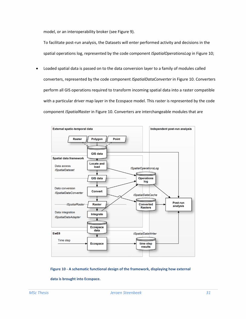
model, or an interoperability broker (see Figure 9).
To facilitate post-run analysis, the Datasets will enter performed activity and decisions in the
spatial operations log, represented by the code component ISpatialOperationsLog in Figure 10;
• Loaded spatial data is passed on to the data conversion layer to a family of modules called
converters, represented by the code component ISpatialDataConverter in Figure 10. Converters
perform all GIS operations required to transform incoming spatial data into a raster compatible
with a particular driver map layer in the Ecospace model. This raster is represented by the code
component ISpatialRaster in Figure 10. Converters are interchangeable modules that are
Figure 10 - A schematic functional design of the framework, displaying how external
data is brought into Ecospace.
MSc Thesis Jeroen Steenbeek 32
capable of performing one type of conversion each, such as different type of raster conversions
and vector to raster conversions.
Converters will log performed spatial operations into the spatial operations log. Additionally, the
rasters that are produced by the converters are stored in a cache that serves to (i) provide the
outcome of conversion steps available for post-run statistical analysis, and (ii) to facilitate
reusing the intermediate data for a next model run which will enhance the performance of the
spatial temporal data framework (not depicted in Figure 10);
• Converted raster data is passed on to the data integration layer to a family of components called
adapters, represented by the code component ISpatialDataAdapter in Figure 10. Adapters
perform the task of placing the loaded and converted raster data into the correct maps of the
Ecospace model, and may trigger Ecospace to perform dedicated tasks to ensure that integrated
data is conrrectly included in the running computations. The Ecospace model will offer an
adapter for every type of map that can be provided with external data.
Adapters will enter their activity in the spatial operations log for post-analysis purposes;
• During Ecospace execution, results are written to a spatial map files via the code component
ISpatialResultWriter. These files can be included in any desired post-run statistical analysis.
The reverse pathway, when Ecospace results are passed through the framework for delivery as GIS data,
is given in Figure 11. This pathway is similar:
• Result maps produced by Ecospace are passed to an adapter for the type of result data. The
adapter encapsulates the map data into a generic ISpatialRaster grid for processing by the
spatial data framework;
• The result grid is received by ISpatialDataConverter converter. Any conversion that needs to be

MSc Thesis Jeroen Steenbeek 33
performed, such as raster-to-vector conversions, will be handled here;
• The converted data is passed to ISpatialDataSet which then makes the data available for
external use by for instance saving the data to a file, to a geodatabase, or by passing the data on
to a model interoperability broker.
Implementation
The implementation of the spatial framework needs to be open to future changes. The system may
require access to new data formats, storage media, and different models which demands flexibility in
adding new ISpatialDataset modules to the framework. New conversion modules may be required if the
Figure 11 - Data exchange framework – producing data.
MSc Thesis Jeroen Steenbeek 34
internal structure of GIS data is incompatible with existing converters, or if different GIS operations are
needed. Additionally, new adapters, operation logs, and result writers may be needed to extend the
capabilities Ecospace itself. Here, the existing EwE6 plug-in structure provides the flexibility that is
needed.
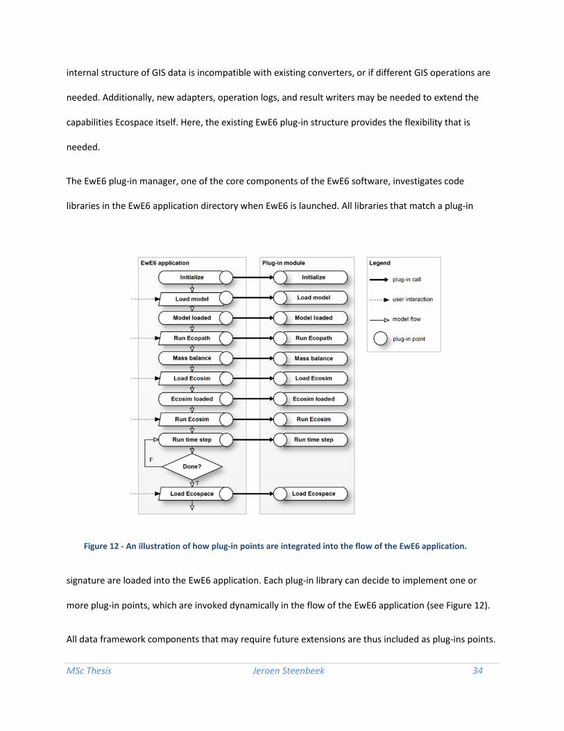
The EwE6 plug-in manager, one of the core components of the EwE6 software, investigates code
libraries in the EwE6 application directory when EwE6 is launched. All libraries that match a plug-in
signature are loaded into the EwE6 application. Each plug-in library can decide to implement one or
more plug-in points, which are invoked dynamically in the flow of the EwE6 application (see Figure 12).
All data framework components that may require future extensions are thus included as plug-ins points.
Figure 12 - An illustration of how plug-in points are integrated into the flow of the EwE6 application.

MSc Thesis Jeroen Steenbeek 35
This gives the spatial data framework the flexibility to incorporate new GIS functionality without
modifications to the EwE6 source code. Even better: the plug-in structure allows addition of spatial data
framework modules by any developer with access to the EwE6 source code.
Example sequence diagram
The interaction diagram in Figure 13 provides an example of how the Ecospace, adapter, dataset,
converter and GIS toolkit collaborate, and how data flows through these objects, in order to bring
external data into the Ecospace model. The dataset here is a hypothetical GIS file reader, and the data
converter in this example performs a hypothetical set of GIS operations to convert a GIS raster into a
format compatible with the Ecospace model. This schematic diagram illustrates the conceptual
interactions only, and is not intended to present a complete overview. For instance, interactions with
the spatial data log and the spatial data cache, as mentioned earlier in this section, are not included.

MSc Thesis Jeroen Steenbeek 36
Figure 13 illustrates the deliberations that will be made by the framework when trying to access external
data. Note that the interaction diagram in Figure 13 shows that Ecospace, the spatial temporal data
framework and the GIS toolkit are physically separate .NET modules. Adapters are embedded within the
EwE6 application because of their deep integration with the Ecospace model. Datasets and converters
are implemented as separate plug-in modules, and different plug-in libraries can utilize different GIS
toolkits if needed. This extra modularity ensures that the EwE approach does not become reliant on
Figure 13 - Interaction diagram, showing how Ecospace, an adapter, a dataset, a converter and a GIS toolkit
communicate to perform the core framework task to read external data.

MSc Thesis Jeroen Steenbeek 37
third-party developed software.
The challenge is now to present this modular framework in a cohesive manner to EwE users in the
prototype. First, a GIS toolkit will be selected in the next section to implement the prototype of the
spatial temporal data framework.
3.2.3 GIS Toolkit
To implement the prototype of the spatial framework a GIS programming toolkit needs to be selected.
In this section, candidate GIS toolkits are reviewed for collaborating with EwE and a toolkit is selected.
Requirements
Several considerations apply when selecting suitable GIS programming toolkits for implementing a
spatial-temporal framework for EwE:
1. Capabilities
A GIS toolkit for Ecospace should support a range of GIS raster, vector and grid data formats and
data connectivity methods common to the environmental sciences. Based on repeated requests
for Ecospace data connectivity, a candidate toolkit must support at least read and write access
to grid file formats netCDF/HDF, ESRI ASCII and binary grid (bdg) files, and GeoTIFF files.
Supported vector file formats should include ESRI ShapeFile, Geography Markup Language
(GML), and elevation data formats such as DEM. At the moment of writing no immediate need
has been expressed to exchange data with common geodatabase formats or geospatial web
services. It would be prudent to assume that future uses of the spatial framework require
facilities to interact with web services and spatial enabled databases such as PostGIS and
Microsoft SQL Server.

MSc Thesis Jeroen Steenbeek 38
A GIS programming toolkit should provide a library of basic spatial operations for vector and
raster datasets. The Ecospace model operates exclusively on gridded data and the GIS toolkit
must support the basic geospatial operations to convert raster and vector data into a format
compatible with EwE.
To process raster datasets for consumption in Ecospace, the candidate toolkit must provide at
least the means to explore the cell values in a raster, and must be able to report the dimensions,
cell size and data type of the raster. Fundamental spatial operations such as merging, extracting
and splitting raster data are needed. In order to convert raster to Ecospace the toolkit must
support means to resample and interpolate raster content using algorithms such as linear
interpolation, kriging, and inverse distance weighting.
In order to process vector data, the toolkit must be able to report the type of vector data in a
spatial set, must be able to loop over features in the vector data, and query and modify feature
attribute data. Fundamental spatial operations such as merging, clipping, and overlaying vector
data are needed. The toolkit should be able to convert vector data to raster by specific attribute
values. Furthermore, the toolkit should be able to perform polygon area calculations.
Last but not least the toolkit should be able to convert spatial data between geographic
projections.
Visualization capabilities are not required for the current version of EwE6 since the application is
shipped with a simple but sufficient map rendering engine (see Figure 3). However, GIS toolkit
visualization capabilities are considered for possible future use;
2. Intellectual property
A GIS programming toolkit should permit distribution with the EwE6 software. The EwE6
desktop software and its source code have been freely available since their inception. Over the

MSc Thesis Jeroen Steenbeek 39
years, several user-developed modifications have been contributed to the approach (e.g.,
Kavanagh et al., 2004; Beecham et al., 2009; Gascuel et al., 2009). With the 2011 foundation of
the Ecopath International Research and Development Consortium a need arose to formalize a
license model for the Ecopath approach. In 2012, the software approach was officially licensed
under the GNU Public License version 2 as true Free and Open Source Software (FOSS). This
license grants any EwE user the freedom to: (i) run the program, regardless of purpose; (ii) study
and adapt the program; (iii) redistribute the software; and (iv) improve the software and to
release these improvements to the public, provided improvements inherit this same license
model. This license model poses restrictions to the GIS programming toolkits for
implementation of the spatial-temporal data framework.
As such, the EwE approach can only incorporate and publicly release FOSS components that are
compatible with the EwE license, thus excluding commercial, paid-for toolkits;
3. Technical environment
A candidate GIS programming toolkit must be compatible with the Microsoft .NET environment,
the platform that used for the EwE6 source code (see section 3.1).
Free open source GIS toolkits implemented in.NET languages such as C# and VB.NET can be
directly integrated in the software development environment of EwE6, which facilitates
development and trouble shooting. For this reason, technical preference is given to .NET-based
GIS toolkits.
The interaction between C and C++ software and .NET applications is limited to the Windows
platform. Efforts are under way to port EwE6 to other operating systems, and a GIS toolkit
written in C or C++ cannot be used outside the Windows environment. C and C++ toolkits may
be useful to construct the framework prototype, and are therefore included in the evaluation.
MSc Thesis Jeroen Steenbeek 40
.NET applications can interact with programs written in Python and Java via wrapper libraries or
via Mono, an open source cross-platform for the .NET framework. Mono, for instance, is the
current platform of choice to enable EwE6 to run on operating systems other than Windows. At
the time of writing the EwE6 user interface is not fully Mono compliant, and implementation of
the spatial framework could not wait for this compliance to be realized. Java and Python GIS
toolkits are evaluated for potential future use;
4. Extensibility
Due to the intended open-ended applicability of the framework, it must be possible to add new
functionality to a candidate GIS toolkit at any moment. Open source software can be extended,
per definition, via modifications to its source code. However, this is rarely a desired option
because this will make source code deviate from publicly and centrally maintained versions,
which could lead to complications when code needs to be synchronized with this central
repository. Therefore, native extensibility features within the toolkit are preferred for toolkits
that offer relatively small sets of core functionality;
5. Support
Active support of a development team, number of individuals participating in software
development, frequency of public releases and updates to source code, and level of
engagement of software developers and users in discussion forms may be indicative of how well
open source software is maintained and how long it may be around (e.g., Ramsey, 2007).
Frequent, continued, and recent activity in these areas is therefore valued in the evaluation.
When reviewing open source GIS software, Ramsey (2007) also takes the width of the developer
community – the number of participating organizations and available funding, among other
factors - into account. However, a number of high profile and broadly supported open GIS
MSc Thesis Jeroen Steenbeek 41
initiatives such as Feature Data Objects and OpenEV seem to have stopped.
Additionally, the completeness and actuality of reference documentation, availability of
discussion groups, and volume of available code examples on the Internet are highly relevant.
Lastly, this review focuses on open source GIS toolkit libraries only. Desktop GIS such as GRASS,
Quantum GIS, SAGA, and uDig, and web-based mapping and analysis GIS solutions such as OpenLayers,
MapServer, and MapBuilder are not consider at this stage. Interoperability to these tools is technically
feasible, but will require complex programming constructs to synchronize and validate the
communication between the framework and the remote GIS. This added complexity will make the
prototype framework difficult to test and comprehend. Hence for the prototype, which aims to
showcase the feasibility of the framework, only GIS toolkits that facilitate direct interaction with .NET
are evaluated.
Reviewed candidate GIS programming toolkits for the spatial temporal data framework are presented in
Annex B. There, for each toolkit the main purpose is listed, along with its license and utilized
programming language. Then, capabilities and support levels are rated to suitability for the EwE spatial
temporal data framework as follows: ̶ (not supported or unsuitable), + (basic support, usable for EwE),
++ (supports all features needed by EwE), +++ (support exceeds needs of EwE), and ? (insufficient
information available for assessment).

MSc Thesis Jeroen Steenbeek 42
Selected toolkit
After careful evaluation (see the comparison chart in Annex B), the open source GIS toolkit DotSpatial
(http://dotspatial.codeplex.com/) was selected. The license of this library is identical to that of EwE6 and
hence poses no obstructions to releases with EwE. DotSpatial is developed in C#, a language of the .NET
family, and can thus be directly integrated in the EwE6 code base.
DotSpatial provides bi-directional access to required raster and vector GIS file formats, and provides
foundation support for connecting to spatial databases and geo web services. Additionally, DotSpatial
has strong map visualization capabilities that may benefit future developments in EwE.
DotSpatial supports modular extension of its capabilities via a plug-in structure similar to that of EwE6,
where plug-in components are automatically recognized and activated when needed.
There is substantial support information for programming DotSpatial available on the Internet. In
particular, discussion forums dedicated to the DotSpatial GIS toolkit refer to a wide range of freely
available code examples. The DotSpatial programming manual is technical but complete. The DotSpatial
source code, which can be obtained for free, includes an extensive set of code projects that
demonstrate how to operate basic and advanced functionalities of DotSpatial.
Lastly, the DotSpatial user community is actively engaged with the developers in discussion forms, and
development activity occurs almost daily. There is a substantial amount of user-contributed C# code
involving DotSpatial programming. The development process is transparent, offering clear milestones
and insight in the evolution of the DotSpatial code base. Lastly, updates to the DotSpatial toolkit are
issued twice per year, which can be considered frequent among open source toolkits. The newest
version of DotSpatial was released a month before this thesis was submitted

MSc Thesis Jeroen Steenbeek 43
(http://dotspatial.codeplex.com/releases/view/87867).
The only downside to DotSpatial is its reliance on the GDAL (Geospatial Data Abstraction Library) for
accessing a range of raster and vector GIS file formats. At time of writing, these GDAL libraries are
included in DotSpatial as traditional Windows code libraries. These libraries are not part of the .NET
family of languages and are only accessible to .NET code via the Windows operating system. These
libraries will not be usable by other operating systems in their current form, and DotSpatial will not be
able to leverage their functionality when EwE is ported to another operating system.
This shortcoming was not deemed prohibitive to using the DotSpatial toolkit for the framework
prototype. An operating system independent version of the EwE6 should not be expected before the
summer of 2013, and present efforts by the DotSpatial developer team indicate that this hiatus may be
solved before then.

MSc Thesis Jeroen Steenbeek 44
“All models are wrong, but some are useful”
- George E. P. Box (1987)
4 Prototype
The prototype of the spatial temporal data framework was implemented using the DotSpatial GIS toolkit
and was designed in accordance with the designs discussed earlier in this section. The main purpose of
the prototype is to demonstrate the feasibility of extending the Ecospace model with a framework of
modular, abstract components that simplify GIS spatial data connectivity. If successful, this framework
will be used for a series of ambitious model interoperability projects waiting to integrate the Ecospace
model in GIS environments such as the Nereus Model (Christensen, 2012). Perhaps the approach utilized
in this framework can be a used as a foundation for simplifying and compartmentalizing complexity in
order to further model interoperability. But let’s introduce the framework first.
The prototype of the spatial temporal framework integrates with the EwE6 user interface in several
locations, such as shown in Figure 14.

MSc Thesis Jeroen Steenbeek 45
Connections
The chain of connected components throughout the spatial data framework can be complicated to
understand, especially for busy academics that just want to “get the biology done”. As such, the chain of
components that connect a spatial map layer to external data is simply referred to as an ‘external data
connection’.
Figure 14 - The EwE6 user interface, with indications to the presence of the external spatial data facilities: (1)
an item in the EwE navigation tree, (2) a configuration option in the Ecospace menu, (3) an indicator beside a
layer in the Ecospace map interface to indicate each layer connected to external data, and (4) an indicator to
notify the user of the number of active external data connections.

MSc Thesis Jeroen Steenbeek 46
Users can manage external data connections from a central user interface displayed in Figure 15. From
this interface users can perform the tasks needed to configure the spatial temporal data framework:
• Select an Ecospace layer for which to configure an external data connection (area 1). Layers
connected to external spatial data connections are indicated with a blue database image;
• Create, configure, and delete datasets, and assign created datasets (area 2) to the Ecospace map
currently selected in (1). Note that the form refers to data sets as connections, which was, after
much deliberation, chosen as a more intuitive term to present to EwE users;
• Assign a converter to the currently selected Ecospace map and connection, and configure the
selected converter (area 3);
Figure 15 - The central interface to manage external data connections to the Ecospace map, showing (1)
Ecospace layers that accept external data connections, (2) elements to manage data sets, and (3) elements to
select and configure converters.
MSc Thesis Jeroen Steenbeek 47
• Additionally, this form provides an option where users can clear any intermediate spatial result
files that have been created and cached by the spatial temporal framework.
Three experimental types of data sets have been built for testing the spatial framework prototype. A
single file dataset facilitate connections to a single geo-spatial file without explicit temporal dimension.
A multi-file dataset allows connections to a time-indexed collection of GIS files. Last, a simulated model
interoperability dataset was created for testing model interoperability capabilities of the framework.
The model interoperability dataset will be used in future research; the multi-file dataset will be briefly
explained to illustrate the workings of the framework. This dataset will also be used extensively in the
case study (see Chapter 5).
The multi-file dataset maintains a time-stamped index to a list of geo-spatial files. Time steps must
correspond to the monthly, first day of the month time steps of Ecospace, for which this type of data set
may provide access.
The modularity of the framework allows datasets to provide configuration user interfaces when needed.
The configuration interface for the multi-file dataset is displayed in Figure 16. Here, users can enter
desriptive data about a dataset, and build a temporal index to spatial files found on a local computer or
a network. Each file is tagged to the first day of a month. Via this date, the dataset will be able to locate
required files when the spatial temporal data framework executes. The multi-file dataset, developed for
this thesis, exclusively utilizes the DotSpatial GIS toolkit to interact with geospatial data files.

MSc Thesis Jeroen Steenbeek 48
Once defined, datasets can be reused for different Ecospace models. Datasets can even be shared
between users in an organization via a local network.
The first converter that was included in the spatial data framework prototype is a direct raster
converter. This type of converter can only operate on incoming raster data, and transforms this raster
via three fundamental GIS raster operations to an Ecospace-compatible grid of cells. First, the converter
performs a projection transformation to conform the data set to the standard Ecospace projection, WGS
84. Secondly, the raster is clipped to the spatial extent of the Ecospace basemap. Lastly, the clipped
Figure 16 - User interface, developed for this thesis, for configuring a data set to a series of spatial-temporal
files. A dataset needs a description (1). Files can be added from folders (2). Every file is tagged by date (3), which
allows the spatial-temporal framework to locate external data when Ecospace executes. The dataset in this
figure is connected to a directory of netCDF files.

MSc Thesis Jeroen Steenbeek 49
raster is converted to a grid of equal number of rows, number of columns, and cell size as defined in the
Ecospace basemap.
The prototype framework requires means for users to assess the spatial and temporal compatibility of
external data with the location and time span of an Ecospace model. This interface is depicted in Figure
17. Here, all active external data connections are presented along the Ecospace run time to show the
temporal overlap between model and external data (area 3 in Figure 17). In the map area (area 1) the
spatial overlap of the model (area 2) with datasets are shown, and users will be alerted if spatial data
Figure 17 – The EwE6 user interface that provides a cursory overview of the spatial and temporal compatibility
of external data with an Ecospace model. The map section (1) of the interface shows the area of the Ecospace
map (2), and provides details for selected data connection and time step (3).

MSc Thesis Jeroen Steenbeek 50
does not overlap or partially overlaps with the model area. The connection selected in Figure 17 utilizes
the global dataset of primary productivity that will be used in the case study (see Chapter 5).
Last, Figure 18 shows the EwE6 interface where the Ecospace model executes. Here, new entries in the
spatial operations can be viewed in the status panel. The spatial operations log is also written to the
hard disk to enable post-run analysis.
Figure 18 – EwE6 interface from where the Ecospace model is executed. The status panel (1) shows an excerpt
from the spatial operations log as produced by the spatial temporal data framework.

MSc Thesis Jeroen Steenbeek 51
“We, the generation that faces the next century, can add
the solemn injunction ‘If we don't do the impossible, we
shall be faced with the unthinkable.’”
- Petra Kelly (Hertsgaard, 1993)
5 Case study
5.1 Introduction
The Northern-Central Adriatic Sea is one of the most productive areas of the Mediterranean Sea and
one of the major fishing grounds in southern Europe. It plays an important role in the economies of
European countries such as Italy, Croatia and Slovenia. However, a dramatic expansion of fisheries has
taken place since early 1970s (Coll et al., 2009, 2010; Fortibuoni et al., 2010; Lotze et al., 2011).
This case study builds on an EwE ecological model representing the Northern-Central Adriatic Sea
ecosystem (Coll et al., 2007), previously fitted to available time series of data from 1975 to 2002 (Coll et
al., 2009, 2010) (see the overview of the fitting procedure in Annex A - Fit to time series procedure), and
from which an Ecospace model had been developed (Fouzai et al., 2012). This model was used to
evaluate the new spatial-temporal framework for Ecospace developed for this thesis. This case study
represents the first application of the new spatial framework applied to Ecospace at a small geographic
scale. While applying the new spatial-temporal framework, the result (both considering data in monthly
time steps and annual time steps) were compared with the original fitted model (Coll et al., 2009) that
had been made spatially explicit using the original version of Ecospace (Fouzai et al., 2012). The aim was
to analyse if results from the ecological model would be modified and would be improved by applying

MSc Thesis Jeroen Steenbeek 52
the new spatial capabilities.
5.2 Methodology
5.2.1 Study area
The study area is located in the Northern-Central Adriatic Sea, geographical sub-area (GSA) 17 of the
General Fisheries Commission for the Mediterranean (GFCM, 2001). The Northern-Central Adriatic Sea is
a semi-enclosed basin located in the northernmost part of the central Mediterranean. The primary
production varies from a productive (potentially eutrophic) shallow northern basin to an oligotrophic
deeper central basin (Zavatarelli et al., 2000). This production is influenced by a large number of rivers
discharging into the basin, particularly the Po River (Artegiani et al., 1997; Zavatarelli et al., 1998; Pinardi
et al., 2006). This area presents clear spatial dynamics of the marine productivity, with higher
productivity in the shallower northern waters and western areas near the coast, and low productivity in
the eastern and southern areas which are deeper.
This area was chosen because of its productivity, ecological and fisheries characteristics (Bombace,
1992) and the availability of previously developed and published ecological models (Coll et al., 2007,
2009; Fouzai et al., 2012). The total area is approximately 55,500 km2, with an average depth of 75 m,
and a maximum depth (in the Pomo Pit) of about 273 m (Figure 19). This area includes all international
waters 12 miles (nm) off the coast of Italy, Slovenia and Croatia. In addition, Italian territorial waters
beyond 3 nautical miles of the western coast (or less than 10 m depth) were included. The area within 3
nm of the Italian coast was excluded because this area is dominated by artisanal fleets and trawling is
banned. The area covered by Slovenian and Croatian territorial waters was excluded from the eastern
part of the study due to lack of data availability.

MSc Thesis Jeroen Steenbeek 53
5.2.2 The ecological model of the Northern-Central Adriatic Sea
The EwE6 software (EwE, Christensen and Walters, 2004) was previously used to develop a trophic
mass-balance model of the Northern-Central Adriatic Sea and to quantify the ecosystem impacts of
fishing (Coll et al., 2007). This model represented the area in the 1990s, and was fitted to data from
1975 to 2002 (Coll et al., 2009, 2010). More recently, a spatial model was developed (Fouzai et al., 2012)
using the spatial module of the EwE6 software, Ecospace, to examine various fishing management
options.
For this case study, the spatial Northern-Central Adriatic model was driven by two spatial-temporal
series of primary production through the framework. Results were compared to the original fitted
Figure 19 - The Northern-Central (NC) Adriatic Sea study area. The light-grey area represents the
spatial coverage of the ecological model available. Current protected areas and biological
conservation zones are also indicated.

MSc Thesis Jeroen Steenbeek 54
spatial-temporal model to assess the impacts of applying external spatial data to a food web model, and
to assess the workings and impact of the spatial temporal framework.
5.2.3 External primary production data
A global, monthly spatial-temporal time series of primary productivity data, derived from the SeaWiFS
sensor with a spatial resolution of 9 x 9 km and covering the period from October 1997 to December
2008, was provided by the Joint Research Centre of the European Commission (JRC) in Ispra, Italy.
The primary production calculation (Mélin and Hoepffner, 2010) is based on a depth-resolved and
wavelength-resolved model following the original formalism described in Platt and Sathyendranath
(1993) and implemented at global scale by Longhurst et al. (1995). At any given location and time, the
model takes into account the total irradiance available for photosynthesis between 400 and 750 nm, the
phytoplankton biomass indexed by the concentration of chlorophyll, as well as the physiological capacity
of phytoplankton organisms to perform photosynthesis. The spatial and temporal changes in
phytoplankton metabolism and its vertical distribution are considered in the model through the
partition of the global ocean into biomes and provinces within each of which some parameters related
to photosynthesis and depth profile of chlorophyll are assigned according to knowledge from field
observations. The primary production estimates obtained at global scale with this approach are broadly
consistent with those from other models (Carr et al., 2006), and its outputs compare favourably with
independent field measurements collected in various parts of the oceans (Friedrichs et al., 2009; Saba et
al., 2011).
The assignment of the photosynthetic parameters PBmax and Ek is achieved by the combined use of a
temperature dependent relationship for the maximum growth rate (Eppley, 1972) and a variable
formulation to retrieve the Carbon-Chlorophyll ratio following the empirical relation of Cloern et al.

MSc Thesis Jeroen Steenbeek 55
(1995). The dataset consists of monthly mean primary production values from October 1997 to
December 2007, and was expressed in grams of carbon per m2 per day. The data in the time series was
stored as a NetCDF file for each monthly, global map, and was reported by NetCDF metadata to be
scaled to log10. Pascal Derycke confirmed this scale, which was applied for ease of display in the GMIS
website (Derycke, 2012), considering that primary production is often considered as following a log-
normal distribution.
This data is available for download through the JRC GMIS (Global Marine Information System) web
portal (http://gmis.jrc.ec.europa.eu).
5.2.4 Configuration of the spatial-temporal data framework
The new spatial framework was applied in a series of steps. First, the Northern-Central Adriatic Ecospace
model , with 42 rows and 50 columns at 0.1° cell size, and fitted to data, was geo-referenced to spatial
extent 11.9° W, 41.6°S, 16.9°E, 45.8°N (Figure 20). The excluded areas, motivated in section 5.2.1 Study
area, are clearly visible as gray cells in this figure.
Secondly, two sets of time series were derived from the JRC primary production data. The original base
10 logarithmic scale of the data did not match the linear scale of primary production in Ecospace and
needed to be scaled. Additionally, an annual average series was needed to assess whether the
ecosystem model - which was not created with explicit seasonal dynamics - would respond differently to
monthly varying and annual averaged external data.

MSc Thesis Jeroen Steenbeek 56
Thus, the following datasets were created:
1. A monthly dataset with linear-scaled primary productivity data, containing a geospatial file for
each month of data, and,
2. An annual average dataset calculated from the monthly rescaled data set, with a geospatial file
for each annual average.
The monthly dataset covers average primary production patterns from October 1997 to December 2007.
The annual dataset covers average primary production patterns from 1998 to 2007. Figures 21 and 22
present these datasets for the study area.
Figure 20 - Ecospace study map of the Northern-Central Adriatic Sea. This map with a reference image
illustrates the spatial fit in the Ecospace maps interface.

MSc Thesis Jeroen Steenbeek 57
Figure 21 –Minimum, maximum, and mean primary production rates for the North-Central Adriatic in the
monthly dataset.
Figure 22 - Minimum, maximum, and mean primary production rates for the North-Central Adriatic in the annual
dataset.
Then, the new spatial-temporal data framework, developed for this thesis, was used to connect the
derived datasets to Ecospace. As mentioned in the discussion of the spatial framework in section 3.2 and

MSc Thesis Jeroen Steenbeek 58
reflected in Figure 23, loading external data through the spatial-temporal framework requires
configuration of three components: a connection, a converter and an adapter (see section 3.2.2).
Figure 23 – A conceptual overview of how the spatial-temporal data framework loads, adjusts, and integrates
spatial data into Ecospace.
Connect
The connection component provides access to the storage medium of the external data. The initial
implementation of the spatial data framework contains only connection components that provide
access to GIS data stored in a wide range of file formats. However, the abstract design of the spatial
framework enables that, in theory, data connections can be programmed to access any external source
of GIS data, such as GIS web services, GIS desktop analytical environments, ecological models that
provide GIS data, etc. For this case study, the file based connection component was used to provide
access to both datasets (Figure 24).
MSc Thesis Jeroen Steenbeek 59
Convert
The converter component performs the set of spatial operations needed to prepare GIS data, acquired
by the connection component, for integration in Ecospace. The initial implementation of the spatial-
temporal framework contains a converter component that only performs a series of simple raster
operations, but the design of the spatial-temporal data framework allows for inclusion of other types of
converters with limited programming effort. For this case study, the simple raster converter was
selected (Figure 24), which first extracts all raster cells that overlap with the spatial area of the Ecospace
model, and then resamples these cells to the Ecospace grid cell size (see Figure 25).
Adapter
Lastly, converted raster data is integrated into a running Ecospace model. Ecospace represents primary
production as a rate relative to the absolute primary production rate defined in the Ecopath model. For
this case study, the JRC data, which stipulated maps of absolute primary production rates, needed
scaling to base Ecopath primary production rates for proper integration into Ecospace.
The primary production data adapter of the spatial data framework requires this scaling factor to be
entered, and provides a means to calculate this option for an external data set. Given that the Ecopath
model represented one year (Coll et al., 2007), this scaling factor was calculated by dividing the annual
averages for the first complete year of data in both datasets by the Ecopath primary production rate
(Figure 24).

MSc Thesis Jeroen Steenbeek 60
Figure 24 – The new user interface, developed for this MSc thesis, to connect sets of external spatial-temporal
data to Ecospace layers.
Based on this configuration, Figure 25 shows how the JRC GMIS primary production data flows through
the spatial-temporal data framework for this case study.
Figure 25 – Flow of GIS data through the spatial-temporal data framework for this case study. GIS data files are
located and loaded, converted to suitable raster data consumption by Ecospace, and then rescaled and copied
into the internal Ecospace data layers.
5.2.5 Zero-impact analysis of the spatial-temporal framework
Prior to running the external primary production datasets through the spatial-temporal data framework,
a zero-impact analysis was performed to ascertain that the framework was capable of correctly
incorporating external data. The primary production map used by Fouzai et al. (2012) was exported to
an ESRI-compatible ASCII raster for the model area. Figure 26 shows this extracted map.

MSc Thesis Jeroen Steenbeek 61
An external data connection to this raster file was created, and was temporally aligned to the model
start date, and the Ecopath-to-Ecospace scaling factor for this file was calculated (Figure 27). This
configuration ensured exact spatial and temporal alignment of an external copy of the primary
Figure 26 - Original relative primary production map in the Ecospace model.
Figure 27 - External data connection to the original primary
production distribution map of Figure 26.

MSc Thesis Jeroen Steenbeek 62
production map originally embedded in the model used by Fouzai et al. (2012). Executing this classic
Ecospace model using this external data map should produce identical - or near-identical results due to
possible numeric precision conversion artifacts - to running the model without this external map data. If
the results are identical, the spatial-temporal data framework correctly performs a zero-impact analysis.
The zero-impact hypothesis was validated by numerically comparing the primary production maps that
Ecospace produces at the end of the first time step. These maps represent the primary production
distribution after one month of food web effects. The classic, fitted to time series model was executed
with and without the zero-impact primary production map, and the resulting primary production maps
at the end of January 1975 were numerically identical (results not shown here). This analysis confirmed
that the framework was able to incorporate original driving data without producing deviating results.
The framework was thus deemed suitable for incorporating the JRC-derived PP datasets.
5.2.6 Spatial scenarios
The Northern-Central Adriatic Ecospace model was then run under three scenarios:
1) A scenario with the classic fitting to time series data, without any forced primary productivity
data (Coll et al., 2009) (original scenario);
2) A scenario with the fitted model to time series data, including the external data connection to
the monthly rescaled PP data set (Figure 21); and
3) A scenario with the fitted model to time series data, including the external data connection to
the annual rescaled PP dataset (Figure 22).
The procedure to read external time series of data into Ecospace (scenarios 2 and 3) was validated by
extracting minimum, maximum and mean primary productivity values for the annual and monthly
datasets for relevant cells in the Ecospace model (see Figure 28). These trends match the patterns
reported by Mozetič et al. (2010) and Cabrini et al. (In press) of decrease in primary productivity in the

MSc Thesis Jeroen Steenbeek 63
last decades in the Northern-Central Adriatic.
Figure 28 – Minimum, maximum, and mean values for the monthly and annual primary production datasets,
extracted by the spatial framework for relevant Ecospace cells.
The scenarios were run from 1975 to 2008 using Ecosim fitted to the original time series data, followed
by the Ecospace module afterwards. These results were then analysed looking at the temporal and
spatial dynamics of phytoplankton and other specific components of the food web (Annex C). The
groups were chosen by taking into account the ecology of different functional groups of the model and
their direct or indirect relationships with phytoplankton (Coll et al., 2007, 2009).
5.3 Results and discussion
Results are presented for the three scenarios: (i) without external spatial-temporal data, (ii) with
monthly spatial-temporal PP data, and (iii) with annual averaged spatial-temporal PP data.
Results are only presented for the phytoplankton group. Analysis of impacts on the entire food web, and

MSc Thesis Jeroen Steenbeek 64
on functional groups others than the phytoplankton group, are supplied in Annex C.
5.3.1 Phytoplankton dynamics
Temporal patterns of phytoplankton biomass
Ecospace produced the following phytoplankton biomass time series, relative to the Ecopath start value,
for each of the three scenarios (Figure 29):
Figure 29 – Predicted relative (final / initial value) biomass of phytoplankton for each of the scenario runs. The
start of SeaWIFS data being read by the modelling framework is indicated by a black vertical line.
The original run of the model, starting in 1975, predicted a steady biomass of phytoplankton from late
1970s to the late 1990s and in the last part of the time series the model showed a slight increase of
phytoplankton that levelled out toward the end of the time series (Figure 29, blue line). On the contrary,
the second scenario, with monthly spatial-temporal PP data, showed high variation of relative biomass
of phytoplankton over time starting from the beginning of the new dataset in 1997 (Figure 29, green

MSc Thesis Jeroen Steenbeek 65
line), in agreement with the monthly PP dataset (Figure 21). The third scenario, with annual averaged
spatial-temporal PP data, showed smaller fluctuations than the second scenario, a slight increase of
phytoplankton biomass from late 1990s to early 2000s and then a slight decline with time (Figure 29, red
line). These declines, predicted using the new framework, are in line with results from the study area
(Cabrini et al., In press; Mozetič et al., 2010) and are quite different from the original model. This
highlights the importance to drive the spatial Ecospace model with external primary production data to
improve the capability of models to better predict realistic ecological patterns and incorporate the
present and future impact of climate change.
Spatial distribution of phytoplankton biomass
The original GMIS PP dataset, as provided by the Joint Research Centre, shows the following spatial
distributions of primary production for 2007 (Figure 30):
Figure 30 - Original dataset distributions of primary production for 2007: (a) December 2007, (b) annual average
for 2007.
The distribution of primary productivity shown in Figure 30 highlights the highly productive northern
areas, and the influence that this production has on the western coast of the northern and central
b a

MSc Thesis Jeroen Steenbeek 66
Adriatic Sea, while the eastern and central areas show less productivity. This is linked with the
oceanography and water circulation of the area (Artegiani et al., 1997; Zavatarelli et al., 1998, 2000).
The spatial results of the original run of the model did not capture the distribution of phytoplankton
biomass particularly well (higher in northern and western areas and lower in southern and eastern areas
(Figure 31a). This is due to a more homogeneous distribution of primary production data from the
model (Figure 26) than the observations in the area (Figure 30). On the contrary, the second scenario,
with monthly spatial-temporal primary productivity data, and the third scenario, with annual averaged
spatial-temporal primary productivity data, better reproduced the expected spatial patterns of
phytoplankton biomass that occur in the area, with less productive regions in the southern and eastern
part of the maps (Figures 31b and 31c).
Figure 31 - Ecospace map showing the distribution of relative biomass of phytoplankton for the last year of the
simulation, 2007. Results are related with the model (a) without external PP data, (b) with monthly PP data, and
(c) with annual PP data.
5.4 Conclusions of the case study
This case study is the first of its kind to drive the spatial and temporal dynamics of the Ecopath trophic
level food web model with spatial-temporal time series, and shows great promise for incorporating GIS
b a c
MSc Thesis Jeroen Steenbeek 67
analysis into food-web models. The zero-impact analysis showed that the spatial-data framework is able
to deliver reliable data into Ecospace. The flexible organization of the framework facilitated calibration
and execution of the Ecospace model with a minimal set of required steps while demonstrating
transparent access to GIS data. Spatial operations such as raster data interpolation and resampling that
were selected in the spatial data framework configuring functioned as expected, seamlessly converting
the JRC data to the spatial extent of the selected Ecospace posing any further demands on the user. A
longitudinal log of spatial operations was produced by the framework, and converted spatial files were
made available for post-analysis enabling for further validation and analysis.
Overall, results of this first implementation of the new spatial framework are satisfactory and by
implementing the new framework biological results of the model improved. The original run of the
model did not predict well the correct temporal and spatial dynamics of primary production for the
period from 1998 to 2007. However, using the new spatial-temporal data framework, the dynamics of
primary producers were in line with their declining trend observed in the recent past (Cabrini et al., In
press; Mozetič et al., 2010). These results highlights the importance to drive the spatial Ecospace model
with external data to improve the capability of models to better predict observed temporal and spatial
patterns of primary producers. Simulations including the external data reproduced more realistic spatial
distribution of phytoplankton and thus yielded more accurate spatial distributions of zooplankton and
other analysed organisms. In addition, changes in the temporal dynamics of phytoplankton biomasses
cascaded up the food web and influenced the dynamics of zooplankton and other organisms of the food
web (see Annex C).

MSc Thesis Jeroen Steenbeek 68
“Chaos is found in greatest abundance wherever order is
being sought. It always defeats order, because it is better
organized.”
- Terry Pratchett, Interesting Times (1994)
6 General discussion
The framework designed, implemented and tested for this thesis was intended as a structural design for
connecting marine ecosystem models to other tools delivering and using geo-spatial data. The objective
of this thesis was not to deliver in-depth GIS-driven ecological assessments, nor was this thesis intended
as an in-depth discussion of geo-spatial analytical capabilities. The principal aim of this thesis was to lay
the foundation of an extensible and dynamic framework for connecting separate marine ecosystem
models through GIS functionality in order to address ecological issues at scales beyond the capabilities
of a single model. The author concludes that this aim has been achieved with the prototype that was
developed during the work.
The developed framework can be further integrated into Ecospace to drive other dynamics of the
model, such as species distributions, fishing dynamics, or habitat degradation scenarios. The framework
can be further extended to connect to other environmental models or specialist GIS environments. The
habitat capacity model (Figure 32), a new development of Ecospace model described in section Annex A,
is an example of a modular model, that, when driven by external temporal and spatial data, will provide
the EwE6 approach with a range of new analytical possibilities.

MSc Thesis Jeroen Steenbeek 69
The prototype implementation of the framework developed here utilizes a limited set of simple GIS
capabilities that served to demonstrate the potential that GIS functionality offers in the framework.
However, the placeholder capabilities are real: data conversions, projection conversions, raster
operations and transparent data delivery methods have shown that the core functionalities of the
framework function as required. The zero-impact analysis, performed in the case study, revealed that
native model data, once externalized and processed through the framework, produces model results
that are identical to the initial model results. This validation indicates that the prototype operations in
the framework function as intended. The framework actually improves the capability of the Ecospace
model to better approximate observed ecosystem dynamics, as was demonstrated with the case study.
The framework has shown to be robust and reliable.
The structure of the framework is extensible and flexible in applicability due to its modular design and
Figure 32 - The habitat capacity model as a modular model. Users can opt to (a) compute capacity from
environmental driver layers, (b) compute capacity from habitats, or (c) bypass options (a) and (b), and directly
derive habitat capacity from external species envelope models. Options (a) and (b) can be employed in
conjunction. Data for (a), (b) and (c) can be either manually entered, or can be driven by the framework.

MSc Thesis Jeroen Steenbeek 70
separation of model interoperability concepts. Utilizing the plug-in structure of the EwE6 software, the
framework can be extended with new capabilities by any programmer familiar with .NET. Datasets can
be written and added to the system to interact with different storage media. New GIS operations can be
included if new conversions are needed, and potentially every Ecospace input map layer can be driven
by external data. The framework presents its modular components in a flexible user interface intended
to provide GIS functionality to non-expert GIS users. The framework is transparent by providing an
overview of intermediate results, which enables validation of intermediate results and statistical
analysis. Additionally, the framework promotes separation of sub-models in an interoperability
environment, which facilitates switching hypothesis in an end-to-end modelling approach.
The author hopes that this conceptually simple and elegant framework may further the discussion
between model developers how to forward end-to-end modelling.
The prototype as presented in this thesis certainly has shortcomings. The current version of the
Ecospace model offers no facilities to read or produce metadata, and self-directed model linkages could
not be explored. This shortcoming of the EwE6 approach will need to be addressed in the future.
There are also potential pitfalls to the modular structure of the framework. Too many modules can lead
to disorder, which may make the framework difficult to use. If this becomes a problem new structures
may have to be added to ensure the framework remains conceptually organized and workable.
Additionally, the modular division of responsibilities, and the consecutive step-wise processing of data
through the framework by different components, may be a larger source of error than if all GIS
interactions and processing steps were executed within a single module. This should be researched in
once the framework is fully utilized. The post-run analysis data that the framework currently provides
will be an essential aid to this end.

MSc Thesis Jeroen Steenbeek 71
“The one who says it cannot be done should never interrupt
the one doing it”
- George Bernard Shaw (attributed)
7 Conclusions and future developments
The combined effect of a changing climate and human exploitation is affecting global marine ecosystems
in ways that we are only beginning to understand. Traditional ecosystem models and Geographic
Information Systems (GIS), indispensable tools to the effort of attaining understanding and exploring
ecosystem dynamics and management options, are not designed to collaborate, which is needed to
address the cascading effects of change through marine ecosystems. Efforts to build such models –
often referred to as end-to-end models - by combining existing ecological models tend to yield rigid
complexes of hypothesis with limited applicability. A flexible system is needed to the construction of
modelling complexes with a focus on model interchangeability, where different hypotheses can be
employed to assess an ecosystem from different points of view. The primary goal of this thesis was to
define that system via GIS technology.
To this end, a literature search was conducted to assess the state of end-to-end ecosystem modelling
approaches, and to explore the capabilities of Geographic Environmental Systems for integrated model
approaches. This provided an overview of successes, shortcomings and needs to integrated ecosystem
modelling efforts.
Next, a flexible spatial-temporal data exchange framework was conceptualized, defined and
implemented in a prototype to allow Ecospace, the spatial model of the EwE ecosystem modelling

MSc Thesis Jeroen Steenbeek 72
approach, to dynamically integrate geospatial-temporal data from any external source into its
computations, and to dynamically provide its results in common spatial data formats for further model
interoperability. For the implementation of the framework a range of GIS programming toolkits were
evaluated. The selected DotSpatial geospatial toolkit successfully provided the essential geo-spatial data
connectivity and geospatial operations to the framework.
The workings of the framework were successfully tested in a case study, where primary production time
series derived from SeaWiFS satellite imagery were chosen to drive the dynamics of the Ecospace food
web. The external data enhanced the predictive capabilities of the Ecospace model, while it allowed
thorough validation of the correct internal workings of the framework.
There are already several promising projects pending to integrate and extend the capabilities of this
newly developed framework. The most recent addition to the Ecospace model, the habitat capacity
model, added combined food web and species distribution envelope assessments to Ecospace, which
will allow for a wide range of new predictive ecosystem dynamics assessments once the habitat capacity
model is connected to external spatial temporal data delivered by the framework.
The framework is currently being integrated in the Nereus Model (Christensen, 2012), an ambitious
inter-academic research project to perform global ocean assessments with an end-to-end model scope.
This project is likely to challenge every capability promised by the new developed framework, requiring
the Ecospace marine food web model to interact with climatological, biochemical and socio-economic
models.
Another project that recently started will focus on generation new Ecospace base maps from external
data sources. This work is performed with partial funding from the National Oceanographic and
Atmospheric Administration (NOAA).

MSc Thesis Jeroen Steenbeek 73
A project currently under consideration involves development of a quantitative methodology for users
to assess the suitability of alternate external GIS data sets to drive a given Ecospace model. Just as
models need to be exchangeable in an end-to-end approach, models should show robustness when
driven by data of similar content but from different sources. Traditionally, Monte Carlo-type uncertainty
analysis are used to test model output sensitivity to inputs, but this is not feasible in model
interoperability scenarios due to computation times of days to months. Future research may be
dedicated to find an indicative measure of fit between two alternate datasets. If this measure can be
found, a relatively quick pre-assessment could save significant effort and lengthy computation times to
discover that datasets are not compatible.
Lastly, Ecopath, Ecosim and Ecospace should acquire the ability to deliver and interpret metadata to
further model interoperability. Research efforts are planned to integrate Ecological Metadata Language
(EML) support into the EwE approach, and include this support into the spatial temporal data framework
developed for this thesis.

MSc Thesis Jeroen Steenbeek 74
8 References
Ainsworth, C., Samhouri, J.F., Busch, D.S., Cheung, W., Dunne, J., and Okey, T. (2011). Potential impacts
of climate change on Northeast Pacific marine foodwebs and fisheries. ICES J. Mar. Sci. 68(6), 1217–
1229.
Appeltans, W., Bouchet, P., Boxshall, G.A., Fauchald, K., Gordon, D.P., Hoeksema, B.W., Poore, G.C.B.,
Van Soest, R.W.M., Stöhr, S., Walter, T.C., et al. (2011). World register of marine species.
http://www.marinespecies.org/ (Accessed August 12, 2012).
Argent, R.M. (2004). An overview of model integration for environmental applications—components,
frameworks and semantics. Environmental Modelling & Software 19(3), 219–234.
Artegiani, A., Paschini, E., Russo, A., Bregant, D., Raicich, F., and Pinardi, N. (1997). The Adriatic Sea
general circulation. Part II: baroclinic circulation structure. Journal of Physical Oceanography 27(8),
1515–1532.
Beecham, J., Mackinson, S., and Aldridge, J. (2009). Dynamic linking of Ecosim and the GOTM
biochemical model using plugins. Fisheries Centre Research Reports 17(3), 134–135.
Bombace, G. (1992). Fisheries of the Adriatic Sea. In Marine Eutrophication and Population Dynamics,
pp. 379–390.
Boumans, R., and Costanza, R. (2007). The multiscale integrated Earth Systems model (MIMES): the
dynamics, modeling and valuation of ecosystem services. Issues in Global Water System Research, 104–
107.
Box, G.E.P., and Draper, N.R. (1987). Empirical model-building and response surfaces. (John Wiley &

MSc Thesis Jeroen Steenbeek 75
Sons).
Cabrini, M., Fornasaro, D., Cossarini, G., Lipizer, M., and Virgilio, D. (In press). Phytoplankton temporal
changes in a coastal northern Adriatic site during the last 25 years. Estuarine, Coastal and Shelf Science.
Carr, M.E., Friedrichs, M.A.M., Schmeltz, M., Noguchi Aita, M., Antoine, D., Arrigo, K.R., Asanuma, I.,
Aumont, O., Barber, R., Behrenfeld, M., et al. (2006). A comparison of global estimates of marine
primary production from ocean color. Deep Sea Research Part II: Topical Studies in Oceanography 53(5-
7), 741–770.
Christensen, V. (2012). Predicting the Future Ocean: The Nereus Program. In 142nd AAAS Annual
Meeting, (Vancouver, Canada).
Christensen, V., Guenette, S., Heymans, J.J., Walters, C.J., Watson, R., Zeller, D., and Pauly, D. (2003).
Hundred-year decline of North Atlantic predatory fishes. Fish and Fisheries 4(1), 1–24.
Christensen, V., and Lai, S. (2007). Ecopath with Ecosim 6: the sequel. The Sea Around Us Project
Newsletter 43(1-4).
Christensen, V., and Maclean, J. (2011). Ecosystem approaches to fisheries: a global perspective
(Cambridge Univ Pr).
Christensen, V., and Pauly, D. (1993). Trophic models of aquatic ecosystems (The WorldFish Center).
Christensen, V., and Walters, C.J. (2004). Ecopath with Ecosim: methods, capabilities and limitations.
Ecological Modelling 172(2-4), 109–139.
Christensen, V., and Walters, C.J. (2005). Using ecosystem modeling for fisheries management: Where
are we. ICES CM 1000, 19.

MSc Thesis Jeroen Steenbeek 76
Christensen, V., and Walters, C.J. (2011). Progress in the use of ecosystem models for fisheries
management. In Ecosystem Approaches to Fisheries: A Global Perspective, V. Christensen, and J.
MacLean, eds. (Cambridge: Cambridge University Press) pp. 189–205.
Cisneros-Montemayor, A., Christensen, V., Arreguín-Sánchez, F., and Sumaila, U.R. (2012). Ecosystem
models for management advice: An analysis of recreational and commercial fisheries policies in Baja
California Sur, Mexico. Ecological Modelling 228(0), 8–16.
Cloern, J.E., Grenz, C., and Vidergar-Lucas, L. (1995). An Empirical Model of the Phytoplankton
Chrlorphyll: Carbon Ratio-the Conversion factor Between Productivity and Growth Rate. Limnology and
Oceanography 40(7), 1313–1321.
Coll, M., Palomera, I., and Tudela, S. (2009). Decadal changes in a NW Mediterranean Sea food web in
relation to fishing exploitation. Ecological Modelling 220(17), 2088–2102.
Coll, M., Piroddi, C., Albouy, C., Lasram, F.B., Cheung, W., Christensen, V., Karpouzi, V., Guilhaumon, F.,
Mouillot, D., Paleczny, M., et al. (2012). The Mediterranean Sea under siege: spatial overlap between
marine biodiversity, cumulative threats and marine reserves. Global Ecology and Biogeography 21(4),
465–480.
Coll, M., Santojanni, A., Palomera, I., and Arneri, E. (2010). Ecosystem assessment of the North-Central
Adriatic Sea: towards a multivariate reference framework. Marine Ecology Progress Series 417, 193–210.
Coll, M., Santojanni, A., Palomera, I., Tudela, S., and Arneri, E. (2007). An ecological model of the
Northern and Central Adriatic Sea: Analysis of ecosystem structure and fishing impacts. Journal of
Marine Systems 67(1-2), 119–154.
Cook, W. (1991). Object-oriented programming versus abstract data types. In Foundations of Object-

MSc Thesis Jeroen Steenbeek 77
Oriented Languages, J. de Bakker, W. de Roever, and G. Rozenberg, eds. (Springer Berlin / Heidelberg)
pp. 151–178.
Couclelis, H. (2003). The certainty of uncertainty: GIS and the limits of geographic knowledge.
Transactions in GIS 7(2), 165–175.
Crosetto, M., and Tarantola, S. (2001). Uncertainty and sensitivity analysis: tools for GIS-based model
implementation. International Journal of Geographical Information Science 15(5), 415–437.
Crosetto, M., Tarantola, S., and Saltelli, A. (2000). Sensitivity and uncertainty analysis in spatial modelling
based on GIS. Agriculture, Ecosystems & Environment 81(1), 71–79.
Derycke, P. (2012). Re: Data required from the JRC (personal communication).
Diaz, H., and Markgraf, V. (2000). El Niño and the Southern Oscillation: multiscale variability and global
and regional impacts (Cambridge Univ Pr).
ECMA International (2012). Standard ECMA-335. http://www.ecma-
international.org/publications/standards/Ecma-335.htm (Accessed August 11, 2012).
Edgar, G.J., Banks, S.A., Brandt, M., Bustamente, R.H., Chiriboga, A., Earle, S.A., Garske, L.E., Glynn, P.W.,
Grove, J.S., and Henderson, S. (2010). El Niño, grazers and fisheries interact to greatly elevate extinction
risk for Galapagos marine species. Global Change Biology 16(10), 151–178.
Emanuel, K. (2005). Increasing destructiveness of tropical cyclones over the past 30 years. Nature
436(7051), 686–688.
Eppley, R.W. (1972). Temperature and phytoplankton growth in the sea. Fish. Bull 70(4), 1063–1085.
Erturk, A., Razinkovas, A., Zemlys, P., Pilkaityte, R., and Gasiunaite, Z. (2008). Linking NPZD and foodweb
MSc Thesis Jeroen Steenbeek 78
models of an estuarine lagoon ecosystem. In US/EU-Baltic International Symposium, 2008 IEEE/OES,
(IEEE) pp. 1–10.
Espinosa-Romero, M.J., Gregr, E., Walters, C.J., Christensen, V., and Chan, K.M.A. (2011). Representing
mediating effects and species reintroductions in Ecopath with Ecosim. Ecological Modelling 222(9),
1569–1579.
Fabry, V.J., Seibel, B.A., Feely, R.A., and Orr, J.C. (2008). Impacts of ocean acidification on marine fauna
and ecosystem processes. ICES Journal of Marine Science: Journal Du Conseil 65(3), 414–432.
Fegraus, E.H., Andelman, S., Jones, M.B., and Schildhauer, M. (2005). Maximizing the value of ecological
data with structured metadata: an introduction to ecological metadata language (EML) and principles
for metadata creation. Bulletin of the Ecological Society of America 86(3), 158–168.
Fennel, W. (2008). Towards bridging biogeochemical and fish-production models. Journal of Marine
Systems 71(1-2), 171–194.
Fortibuoni, T., Libralato, S., Raicevich, S., Giovanardi, O., and Solidoro, C. (2010). Coding early naturalists’
accounts into long-term fish community changes in the Adriatic Sea (1800–2000). PloS One 5(11),
e15502.
Fouzai, N., Coll, M., Palomera, I., Santojanni, A., Arneri, E., and Christensen, V. (2012). Fishing
management scenarios to rebuild exploited resources and ecosystems of the Northern-Central Adriatic
(Mediterranean Sea). Journal of Marine Systems 102-104, 39–51.
Francis, T., Levin, P.S., and Harvey, C.J. (2011). The perils and promise of futures analysis in marine
ecosystem-based management. Marine Policy 35(5), 675–681.

MSc Thesis Jeroen Steenbeek 79
Friedrichs, M.A.M., Carr, M., Barber, R., Scardi, M., Antoine, A., Armstrong, R., Asanuma, I., Behrenfeld,
M., Buitenhuis, E.T., Chai, F., et al. (2009). Assessing the uncertainties of model estimates of primary
productivity in the tropical Pacific Ocean. Journal of Marine Systems 76(1-2), 113–133.
Froese, R., and Pauly, D. (2010). FishBase (Vancouver, Canada: Fisheries Centre, University of British
Columbia).
Fulton, E.A. (2010). Approaches to end-to-end ecosystem models. Journal of Marine Systems 81(1-2),
171–183.
Fulton, E.A., Gray, R., Sporcic, M., Scott, R., and Hepburn, M. (2009). Challenges of crossing scales and
drivers in modelling marine systems. (Cairns, Australia).
Fulton, E.A., Smith, A.D.M., and Johnson, C.R. (2004). Effects of spatial resolution on the performance
and interpretation of marine ecosystem models. Ecological Modelling 176(1-2), 27–42.
Gallagher, J., Potter, N., and Jones, M.B. (2010). Common Patterns with End-to-end Interoperability for
Data Access. In AGU Fall Meeting Abstracts, p. 1080.
Gamma, E., Helm, R., Johnson, R., and Vlissides, J. (1994). Design Patterns: Elements of Reusable Object-
Oriented Software (Addison-Wesley Professional).
Gascuel, D., Tremblay-Boyer, L., and Pauly, D. (2009). EcoTroph (ET): a trophic level based software for
assessing the impacts of fishing on aquatic ecosystems. Fisheries Centre Research Reports 17(1).
GFCM (2001). Report of the Twenty-sixth Session: Lacco Ameno, Ischia, Italy, 10-13 September 2001
(FAO).
Gil, I.S., Sheldon, W., Schmidt, T., Servilla, M., Aguilar, R., Gries, C., Gray, T., Field, D., Cole, J., Pan, J.Y., et

MSc Thesis Jeroen Steenbeek 80
al. (2008). Defining linkages between the GSC and NSF’s LTER program: how the Ecological Metadata
Language (EML) relates to GCDML and other outcomes. OMICS A Journal of Integrative Biology 12(2),
151–156.
Goodchild, M.F., Parks, B.O., and Steyaert, L.T. (1993). Environmental modeling with GIS (Oxford
University Press, USA).
Grassle, J.F. (2000). The Ocean Biogeographic Information System (OBIS): an on-line, worldwide atlas for
accessing, modeling and mapping marine biological data in a multidimensional geographic context.
Oceanography 13(3).
Gray, R., Fulton, E.A., Little, L., and Scott, R. (2006). Operating Model Specification Within an Agent
Based Framework (CSIRO, Hobart, Tasmania).
Greenberg, J., White, H.C., Carrier, S., and Scherle, R. (2009). A metadata best practice for a scientific
data repository. Journal of Library Metadata 9(3-4), 194–212.
Hansen, J., Sato, M., Ruedy, R., Lo, K., Lea, D.W., and Medina-Elizade, M. (2006). Global temperature
change. Proceedings of the National Academy of Sciences 103(39), 14288–14293.
Hertsgaard, M. (1993). Who killed Petra Kelly? Vanity Fair (New York).
Heuvelink, G.B.M. (1998). Error propagation in environmental modelling with GIS (London: Taylor &
Francis).
Hilborn, R., and Walters, C.J. (1992). Quantitative fisheries stock assessment: choice, dynamics, and
uncertainty. (London: Chapman & Hall).
Jacobs, G., Hurlburt, H., Kindle, J., Metzger, E., Mitchell, J., Teague, W., and Wallcraft, A. (1994). Decade-

MSc Thesis Jeroen Steenbeek 81
scale trans-Pacific propagation and warming effects of an El Niño anomaly. Nature 370, 360–363.
Jager, H.I., and King, A.W. (2004). Spatial Uncertainty and Ecological Models. Ecosystems 7(8), 841–847.
Jolma, A., Ames, D.P., Horning, N., Mitasova, H., Neteler, M., Racicot, A., and Sutton, T. (2008). Free and
Open Source Geospatial Tools for Environmental Modelling and Management. Developments in
Integrated Environmental Assessment 3, 163–180.
Kacprzyk, J. (2010). Uncertainty Approaches for Spatial Data Modeling and Processing: A Decision
Support Perspective (Springer Verlag).
Kavanagh, P., Newlands, N., Christensen, V., and Pauly, D. (2004). Automated parameter optimization
for Ecopath ecosystem models. Ecological Modelling 172(2), 141–149.
Kearney, K.A., Stock, C., Aydin, K., and Sarmiento, J.L. (2012). Coupling planktonic ecosystem and
fisheries food web models for a pelagic ecosystem: Description and validation for the subarctic Pacific.
Ecological Modelling 237–238, 43–62.
Kishi, M.J., Kashiwai, M., Ware, D.M., Megrey, B.A., Eslinger, D.L., Werner, F.E., Noguchi-Aita, M.,
Azumaya, T., Fujii, M., Hashimoto, S., et al. (2007). NEMURO–a lower trophic level model for the North
Pacific marine ecosystem. Ecological Modelling 202(1-2), 12–25.
Leslie, H.M., and McLeod, K.L. (2007). Confronting the challenges of implementing marine ecosystem-
based management. Frontiers in Ecology and the Environment 5(10), 540–548.
Levin, P.S., Fogarty, M.J., Murawski, S.A., and Fluharty, D. (2009). Integrated Ecosystem Assessments:
Developing the Scientific Basis for Ecosystem-Based Management of the Ocean. PLoS Biol 7(1),
e1000014.
MSc Thesis Jeroen Steenbeek 82
Levin, S.A. (1992). The Problem of Pattern and Scale in Ecology: The Robert H. MacArthur Award Lecture.
Ecology 73(6), 1943.
Libralato, S., and Solidoro, C. (2009). Bridging biogeochemical and food web models for an End-to-End
representation of marine ecosystem dynamics: The Venice lagoon case study. Ecological Modelling
220(21), 2960–2971.
Longhurst, A., Sathyendranath, S., Platt, T., and Caverhill, C. (1995). An estimate of global primary
production in the ocean from satellite radiometer data. Journal of Plankton Research 17(6), 1245–1271.
Loos, S.A. (2011). Marxan Analyses and Prioritization of the Central Interior Ecoregional Assessment. BC
Journal of Ecosystems and Management 12(1).
Lotze, H.K., Coll, M., and Dunne, J.A. (2011). Historical changes in marine resources, food-web structure
and ecosystem functioning in the Adriatic sea, Mediterranean. Ecosystems 14(2), 198–222.
Manso, M.A., and Wachowicz, M. (2009). GIS Design: A Review of Current Issues in Interoperability.
Geography Compass 3(3), 1105–1124.
Martell, S.J., Essington, T.E., Lessard, B., Kitchell, J.F., Walters, C.J., and Boggs, C.H. (2005). Interactions
of productivity, predation risk, and fishing effort in the efficacy of marine protected areas for the central
Pacific. Canadian Journal of Fisheries and Aquatic Sciences 62(6), 1320–1336.
Martell, S.J.D., Beattie, A.I., Walters, C.J., Nayar, T., and Briese, R. (2002). Simulating fisheries
management strategies in the Strait of Georgia ecosystem using Ecopath and Ecosim. The Use of
Ecosystem Models to Investigate Multispecies Management Strategies for Capture Fisheries 10(2), 16–
23.

MSc Thesis Jeroen Steenbeek 83
Mélin, F., and Hoepffner, N. (2010). Monitoring Phytoplankton Productivity from Satellite - An Aid to
Marine Resources Management. (EU PRESPO Project and International Ocean Colour Coordinating
group).
Michener, W.K. (2006). Meta-information concepts for ecological data management. Ecological
Informatics 1(1), 3–7.
Michener, W.K., Brunt, J.W., Helly, J.J., Kirchner, T.B., and Stafford, S.G. (1997). Nongeospatial metadata
for the ecological sciences. Ecological Applications 7(1), 330–342.
Mozetič, P., Solidoro, C., Cossarini, G., Socal, G., Precali, R., Francé, J., Bianchi, F., De Vittor, C., Smodlaka,
N., and Fonda Umani, S. (2010). Recent trends towards oligotrophication of the northern Adriatic:
evidence from chlorophyll a time series. Estuaries and Coasts 33(2), 362–375.
Nelson, E.J., and Daily, G.C. (2010). Modelling ecosystem services in terrestrial systems. F1000 Biology
Reports 2(53).
NOAA (2007). ECOPATH Modeling: Precursor to an Ecosystem Approach to Fisheries Management.
http://celebrating200years.noaa.gov/breakthroughs/ecopath/welcome.html (Accessed August 26,
2012).
Orr, J.C., Fabry, V.J., Aumont, O., Bopp, L., Doney, S.C., Feely, R.A., Gnanadesikan, A., Gruber, N., Ishida,
A., Joos, F., et al. (2005). Anthropogenic ocean acidification over the twenty-first century and its impact
on calcifying organisms. Nature 437(7059), 681–686.
Pauly, D., Christensen, V., Dalsgaard, J., Froese, R., and Torres, F. (1998). Fishing down marine food
webs. Science 279(5352), 860.

MSc Thesis Jeroen Steenbeek 84
Pauly, D., Christensen, V., and Walters, C. (2000). Ecopath, Ecosim, and Ecospace as tools for evaluating
ecosystem impact of fisheries. ICES Journal of Marine Science: Journal Du Conseil 57(3), 697–706.
Pauly, D. (2010). The ocean’s shifting baseline.
http://www.ted.com/talks/daniel_pauly_the_ocean_s_shifting_baseline.html (Accessed June 9, 2012).
Pinardi, N., Arneri, E., Crise, A., Ravaioli, M., and Zavatarelli, M. (2006). The physical, sedimentary and
ecological structure and variability of shelf areas in the Mediterranean sea (27). The Sea 14, 1243–1330.
Plaganyí, E.P. (2007). Models for an ecosystem approach to fisheries. FAO Fisheries Technical Paper
(FAO).
Platt, T., and Sathyendranath, S. (1993). Estimators of primary production for interpretation of remotely
sensed data on ocean color. Journal of Geophysical Research 98(C8), 14561–14.
Pratchett, T. (1994). Interesting Times (London: Victor Gollancz).
ProQuest (2012). ASFA: Aquatic Sciences and Fisheries Abstracts. http://search.proquest.com/asfa/
(Accessed August 20, 2012).
Ramsey, P. (2007). A survey of open source GIS. In The 2007 FOSS4G Conference, (Victoria, Canada).
Rose, K.A. (2012). End-to-end models for marine ecosystems: Are we on the precipice of a significant
advance or just putting lipstick on a pig? Scientia Marina 76(1), 195–201.
Rose, K.A., Icarus Allen, J., Artioli, Y., Barange, M., Blackford, J., Carlotti, F., Cropp, R., Daewel, U.,
Edwards, K., Flynn, K., et al. (2010). End-To-End Models for the Analysis of Marine Ecosystems:
Challenges, Issues, and Next Steps. Marine and Coastal Fisheries: Dynamics, Management, and
Ecosystem Science 2(1), 115–130.

MSc Thesis Jeroen Steenbeek 85
Saba, V.S., Friedrichs, M.A.M., Antoine, D., Armstrong, R.A., Asanuma, I., Behrenfeld, M.J., Ciotti, A.M.,
Dowell, M., Hoepffner, N., Hyde, K.J.W., et al. (2011). An evaluation of ocean color model estimates of
marine primary productivity in coastal and pelagic regions across the globe. Biogeosciences 8(2), 489–
503.
Scherle, R., Carrier, S., Greenberg, J., Lapp, H., Thompson, A., Vision, T., and White, H. (2008). Building
support for a discipline-based data repository. (Southampton, United Kingdom).
Shin, Y.J., and Cury, P. (2001). Exploring fish community dynamics through size-dependent trophic
interactions using a spatialized individual-based model. Aquating Living Resources 14(2), 16.
Shin, Y.J., Travers, M., and Maury, O. (2010). Coupling low and high trophic levels models: Towards a
pathways-orientated approach for end-to-end models. Progress in Oceanography 84(1-2), 105–112.
Solimini, A.G., Ptacnik, R., and Cardoso, A.C. (2009). Towards holistic assessment of the functioning of
ecosystems under the Water Framework Directive. TrAC Trends in Analytical Chemistry 28(2), 143–149.
Steele, J.H., and Ruzicka, J.J. (2011). Constructing end-to-end models using ECOPATH data. Journal of
Marine Systems 87, 227–238.
Stock, C., Alexander, M.A., Bond, N.A., Brander, K.M., Cheung, W., Curchitser, E.N., Delworth, T.L.,
Dunne, J., Griffies, S.M., and Haltuch, M.A. (2011). On the use of IPCC-class models to assess the impact
of climate on living marine resources. Progress in Oceanography 88(1-4), 1–27.
Travers, M., Shin, Y.J., Jennings, S., and Cury, P. (2007). Towards end-to-end models for investigating the
effects of climate and fishing in marine ecosystems. Progress in Oceanography 75(4), 751–770.
Valavanis, V.D. (2002). Geographic Information Systems in Oceanography and Fisheries (London: Taylor

MSc Thesis Jeroen Steenbeek 86
& Francis).
Waage, S., Stewart, E., and Armstrong, K. (2008). Measuring corporate impact on ecosystems: A
comprehensive review of new tools. San Francisco, CA, Business for Social Responsibility 18.
Walters, C. (2000). Impacts of dispersal, ecological interactions, and fishing effort dynamics on efficacy
of marine protected areas: how large should protected areas be? Bulletin of Marine Science 66(3), 745–
757.
Walters, C.J., Christensen, V., and Pauly, D. (1997). Structuring dynamic models of exploited ecosystems
from trophic mass-balance assessments. Reviews in Fish Biology and Fisheries 7(2), 139–172.
Walters, C.J., Christensen, V., Walters, W., and Rose, K.A. (2010). Representation of multistanza life
histories in Ecospace models for spatial organization of ecosystem trophic interaction patterns. Bulletin
of Marine Science 86(2), 439–459.
Walters, C.J., Pauly, D., and Christensen, V. (1999). Ecospace: Prediction of Mesoscale Spatial Patterns in
Trophic Relationships of Exploited Ecosystems, with Emphasis on the Impacts of Marine Protected
Areas. Ecosystems 2(6), 539–554.
Webster, P.J., Holland, G.J., Curry, J.A., and Chang, H.R. (2005). Changes in tropical cyclone number,
duration, and intensity in a warming environment. Science 309(5742), 1844.
Wesseling, C., Karssenberg, D., Burrough, P., and van Deursen, W. (1996). Integrating dynamic
environmental models in GIS: the development of a Dynamic Modelling language. Transactions in GIS
1(1), 40–48.
Whitlock, M.C. (2011). Data archiving in ecology and evolution: best practices. Trends in Ecology &
MSc Thesis Jeroen Steenbeek 87
Evolution 26(2), 61–65.
Zavatarelli, M., Baretta, J.W., Baretta-Bekker, J.G., and Pinardi, N. (2000). The dynamics of the Adriatic
Sea ecosystem. An idealized model study. Deep Sea Research Part I: Oceanographic Research Papers
47(5), 937–970.
Zavatarelli, M., Raicich, F., Bregant, D., Russo, A., and Artegiani, A. (1998). Climatological biogeochemical
characteristics of the Adriatic Sea. Journal of Marine Systems 18(1), 227–263.

MSc Thesis Jeroen Steenbeek 88
Annex A Principles of the Ecopath with Ecosim approach
This annex provides supplementary information to the introduction of EwE6 in section 3.1.
The Ecopath with Ecosim (EwE) approach was first proposed and realized as a case study of the French
Frigate Shoals (Polovina, 1984). This publication introduced path analysis to the field of ecology, where
primary producers such as aquatic plants and phytoplankton convert radiant energy into organic
substances which form the nutritional foundation for marine life. Via chains of predation this energy
travels along identifiable path ways through a food web. The mass-balance constraint that Polovina
included in this model stated that the total amount of energy that transfers through a food-web – but
that also passes through individual organisms during their life cycles or gets exported as catches - must
balance, since energy is neither created nor destroyed. The combination of path analysis and mass-
balance yielded a model that, based on a relatively small number of input parameters, was scalable
enough to capture the characteristics of individual ecosystems, and proved to be surprisingly accurate
despite its perceived simplicity (Christensen and Walters, 2004).
The simple principles and relative light data input requirements were instrumental to the wide
adaptation of the approach, which arrived timely to the need for a common yet flexible model to marine
ecosystem assessment.
A.1 Ecopath
The core model of the EwE6 approach and previous versions is the Ecopath model (Christensen and
Pauly, 1993; Pauly et al., 2000; Christensen and Walters, 2004). In Ecopath, organisms of similar
population dynamics and ecological function are numerically combined into functional groups (also
referred to as groups or pools), with the exception of species that are deemed of significant importance

MSc Thesis Jeroen Steenbeek 89
to the modelled ecosystem which are either represented as individual groups or as a group for each
significant life stage. The Ecopath model is based on the presumption that every ecosystem is in a state
where the total amount of incoming and outgoing energy balances. By considering a relatively small set
of input parameters that represent the dynamics of, and interactions between, functional groups in an
ecosystem, Ecopath validates this assumption in a mass-balance assessment.
The Ecopath model describes average energy flows over a given time period which is typically one year
(Christensen and Walters, 2004).
In its foundation, the linear equations that constitute to the Ecopath mass-balance assessment are quite
simple. Since the system is assumed to be in a steady state, groups must also be in a steady state, thus
the total energy input of a group must equal its output. This is expressed in Ecopath as:
𝑄 = 𝑃 + 𝑅 + 𝑈 (eq. 1)
Q is consumption of a group, P its production, R the amount of energy that it respires, and U the amount
of unassimilated food. The production P of a group is defined as:
𝑃 = 𝑀2 ∙ 𝐵 + 𝐸 + 𝐵𝐴 + 𝑌 + 𝑀0 ∙ 𝐵 (eq. 2)
Here, B is the biomass of a group for the Ecopath time period, E is the net migration of this group in the
system, BA is the biomass accumulation in the ecosystem, Y is the catch, M2 is the rate of predation
mortality exerted onto the group and M0 is its other mortality rate. Predation mortality M2 is the total
amount of group (i) that is eaten by other groups (j), and is expressed relative to the biomass of the
group as:

MSc Thesis Jeroen Steenbeek 90
𝑀2𝑖 = �𝑄𝑗 ∙ 𝐷𝐶𝑗𝑖
𝐵𝑖
𝑛
𝑗=1
(eq. 3)
The term Q indicates the consumption rate of predator (j) and DCji is the fraction of the diet of predator
(j) contributed by group (i).
The other mortality M0 term in equation 1 aggregates all mortality not related to predation such as
mortality due to parasites or diseases and is computed as:
𝑀0𝑖 = 𝑃𝑖 ∙ (1 − 𝐸𝐸𝑖) 𝐵𝑖⁄ (eq. 4)
Here, the ecotrophic efficiency coefficient EE represents the production of group (i) that is used within,
or removed from the system – i.e. the mortality that is “explained” by the model. By combining the
equations above, the mass balance constraints now determine that every group (i) can be represented
by the following equation:
𝐵𝑖 �𝑃𝐵�𝑖∙ 𝐸𝐸𝑖 − 𝑌𝑖 − 𝐸𝑖 − 𝐵𝐴𝑖 −�𝑄𝑗
𝑛
𝑗=1
∙ 𝐷𝐶𝑗𝑖 = 0 (eq. 5)
This, in essence, is the heart of the Ecopath model.
Equation (5) shows that only three of the four core parameters - biomass (B), production rate (P/B),
consumption rate (Q/B), and ecotrophic efficiency (EE) -need to be entered; the mass balance constraint
allows for estimation of the missing term. Not coincidentally, the terms P/B, Q/B and Y are derived from
traditional ecological analysis and population dynamics, ensuring that parameter data is widely
available, which has contributed to the wide adaptation of the approach.

MSc Thesis Jeroen Steenbeek 91
Ecopath also supports inclusion of fishing efforts and fishing discards into the mass balance assessment
(see term M0 in equation 4), and contains delay-difference age/size structures for key populations. In-
depth explanations can be found in Pauly et al. (2000), Christensen and Walters (2004), Christensen et
al. (2009), and Walters et al. (2010).
The Ecopath model facilitated its use for analyses such as ecological networks (Christensen and Pauly,
1992; Heymans and Baird, 2000), primary production required (Pauly et al., 1995), and mass-balance
assessments of ecosystems world-wide. NOAA, the National Oceanic and Atmospheric Administration,
celebrated the approach one of the ten biggest scientific breakthroughs in its 200 year existence (NOAA,
2007). Most relevant to this thesis, though, is that the static mass-balance snapshot model Ecopath
became the precursor to the time-dynamic model Ecosim (Walters et al., 1997; Walters, 2000) and the
time-space dynamic model Ecospace (Walters et al., 1999, 2010).
A.2 Ecosim
In 1995 the Ecosim module was added to the desktop software for exploring past and future impacts of
fishing and environmental disturbances over time. Ecosim re-expresses the linear Ecopath equations as
a set of differential equations and solves these for regular time intervals for any given time period,
under the assumption that biomasses and the ability of any group to produce and consume are variable.
The core equation of Ecosim is based on Ecopath model parameters and applies the mass-balance over
time:
𝑑𝐵𝑖𝑑𝑡
=𝑃𝑄∙�𝑄𝑗𝑖 −�𝑄𝑖𝑗 + 𝐼𝑖 − (𝑀0𝑖 + 𝐹𝑖 + 𝑒𝑖) ∙ 𝐵𝑖 (eq. 6)
where dBi/dt represents the growth rate of group (i) over the time interval dt in terms of its biomass Bi.

MSc Thesis Jeroen Steenbeek 92
The consumption rate terms Qji and Qij are computed based on the foraging arena concept.
A.2.1 Foraging arena
Central in the Ecosim model are dynamic effects of predation (Walters et al., 1997). Traditional
predation interactions, based on biomasses of predator, prey and diet rates (known as ‘mass action’ or
Lotka-Volterra assumptions) assume predation to be a function of abundance in predator and prey. Such
models could be made to work for small population numbers, but tended to be highly unstable for more
complex populations. These models assumed near-linear increases of predators and extinctions of prey,
an effect long known not to happen in reality (e.g., Pielou, 1981), even with high predator abundances
(Pauly et al., 2000).
The foraging arena theory was proposed in
Ecosim to better approximate reality, and avoid
the instabilities of Lotka-Volterra based
models. The foraging theory, which could be
best thought of as a “risk management
behaviour model” (Walters et al., 1999),
numerically represents the fact that at a given
moment only a fraction of prey biomass in a
given aquatic ecosystem is available to a
certain predator because of behaviours and
physical mechanisms (Walters et al., 1997): fish spend significant amounts of time hiding from
predators, and are mainly vulnerable to predation when foraging for food themselves (Figure A-1).
Numerically, Ecosim divides biomass B of prey group (i) into a portion that is available (Vi), and a portion
Figure A-1 - The foraging arena theory: only a portion of
prey biomass is available to predation at any given
moment.
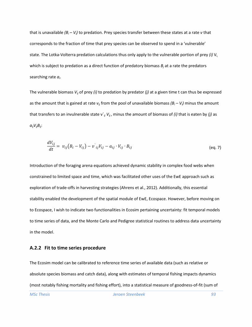
MSc Thesis Jeroen Steenbeek 93
that is unavailable (Bi – Vi) to predation. Prey species transfer between these states at a rate v that
corresponds to the fraction of time that prey species can be observed to spend in a ‘vulnerable’
state. The Lotka-Volterra predation calculations thus only apply to the vulnerable portion of prey (i) Vi,
which is subject to predation as a direct function of predatory biomass Bj at a rate the predators
searching rate ai.
The vulnerable biomass Vij of prey (i) to predation by predator (j) at a given time t can thus be expressed
as the amount that is gained at rate vij from the pool of unavailable biomass (Bi – Vi) minus the amount
that transfers to an invulnerable state v`ij Vij , minus the amount of biomass of (i) that is eaten by (j) as
aijVijBij:
𝑑𝑉𝑖𝑗𝑑𝑡
= 𝑣𝑖𝑗�𝐵𝑖 − 𝑉𝑖𝑗� − 𝑣 `𝑖𝑗𝑉𝑖𝑗 − 𝑎𝑖𝑗 ∙ 𝑉𝑖𝑗 ∙ 𝐵𝑖𝑗 (eq. 7)
Introduction of the foraging arena equations achieved dynamic stability in complex food webs when
constrained to limited space and time, which was facilitated other uses of the EwE approach such as
exploration of trade-offs in harvesting strategies (Ahrens et al., 2012). Additionally, this essential
stability enabled the development of the spatial module of EwE, Ecospace. However, before moving on
to Ecospace, I wish to indicate two functionalities in Ecosim pertaining uncertainty: fit temporal models
to time series of data, and the Monte Carlo and Pedigree statistical routines to address data uncertainty
in the model.
A.2.2 Fit to time series procedure
The Ecosim model can be calibrated to reference time series of available data (such as relative or
absolute species biomass and catch data), along with estimates of temporal fishing impacts dynamics
(most notably fishing mortality and fishing effort), into a statistical measure of goodness-of-fit (sum of

MSc Thesis Jeroen Steenbeek 94
squared deviations, SS) that is frequently used as a metric for assessing the fit of the model to real data.
This measure of fit compares model predictions to observed data when available, and is expressed as a
weighted sum of squared deviations of log observed catches and biomasses from log predicted catches
and biomasses (Christensen and Walters, 2004; Shannon et al., 2004; Coll et al., 2008).
During the fitting, Ecosim calculates the values for vulnerabilities (from equation 7) to minimize SS
deviations between predicted and observed parameters. The model can also calculate an environmental
anomaly obtained from the calibration process (which represents a multiplier of the initial Ecopath value
of primary producer groups’ growth P/B), and that also is used to minimize SS deviations. This anomaly
can be then correlated with the environmental data available.
A.2.3 Parameter uncertainty
To address the issue of parameter uncertainty, the Ecosim approach features a Monte Carlo statistical
test that draws random input variables to Ecopath from user-provided frequency distributions. When
ran for a user-defined number of trials, outcomes are evaluated using the mass-balance constraint and
physiological constraints as computed by Ecosim against reference time series (such as used to fit the
time series, for example). Expressed in sum of squared deviations (SS) values, the best fitting trial is
retained and can be applied to the Ecopath model as new input values for its core variables P/B, Q/B, B,
and EE.
This methodology can be used to estimate confident intervals in output parameters of the model.
Users of the approach can also express input parameter confidence by using the pedigree system
integrated in Ecopath. Serving a dual purpose, this system can be used to (i) describe the origin of data
and (ii) provide a measure of data confidence based on their origin. The confidence intervals provided as

MSc Thesis Jeroen Steenbeek 95
part of the pedigree information can be directly connected to determine the frequency distributions
used by the Monte Carlo approach (Pauly et al., 2000; Christensen and Walters, 2004).
The pedigree index is used by model users to compare the quality of their model to the overall
distribution of pedigree indices of available models, such as published in Morisette (2007).
A.3 Ecospace
The third core module of EwE is the spatial/temporal model Ecospace, a spatially explicit multi-species
ecosystem model (Walters et al., 1999, 2010; Christensen et al., 2003; Christensen and Maclean, 2011).
Ecospace has been widely applied to quantify the spatial impacts on marine species due to fishing, and
to analyse the outcomes of management options such as the establishment of marine protected areas
and its impact in terms of spatial distribution of marine species and fishing effort (e.g., Walters, 2000;
Martell et al., 2005; Walters et al., 2010; Fouzai et al., 2012). It can also be used to develop spatial
optimization routines (Christensen et al., 2009) and assess the impact of climate change by linking the
Ecospace model with low trophic level models (Fulton, 2011).
Ecospace is primarily designed to assess the spatial cascade effects of policy screening approaches,
rather than to be used for detailed quantitative descriptions (Walters et al., 1999).
The Ecospace model was built to model biomass interactions within an ecosystem across a two-
dimensional grid over time. Ecospace distributes Ecopath biomass values of functional groups across a
grid of equally sized cells, and uses the Ecosim equations to model how biomasses vary within each cell
in the grid over time by taking trophic interactions, fishing and species movement into account.
Beside a mass-balanced Ecopath model and an Ecosim configuration, the Ecospace model requires the
following minimal set of inputs:

MSc Thesis Jeroen Steenbeek 96
• Definition of a so-called basemap, which identifies the spatial bounds, number of rows, and
number of columns of an Ecospace model grid. The temporal resolution of an Ecospace model is
dictated by an underlying Ecosim model (Walters et al., 1999).
• A depth map, identifying water cells (expressed as positive, non-zero depths) and land cells (all
other values). Note that the terms depth, land, and water are used in a metaphorical sense.
Water cells merely serve to identify in which cells relevant biological interactions occur. Usable
terrestrial-based Ecospace applications have successfully switched the land/water concepts
without noticeable side effects (e.g., Krebs et al., 2009). Depth is expressed in meters (Walters
et al., 1999).
• A relative primary productivity map that identifies primary productivity variations across the
basemap. The default map in an Ecospace map assumes a homogenous distribution of primary
productivity that can be changed to account for localized variations in productivity (Walters et
al., 1999).
When the Ecospace model initiates, a scaling factor is calculated by dividing the sum of P/B
values in the Ecospace map by the number of water cells and the Ecopath P/B ratio. This scaling
factor is then used to distribute Ecopath primary productivity values across the Ecospace map.
Throughout an Ecospace model run this productivity pattern is kept constant, and is used to
spatially distribute fluctuations in primary productivity.
Additionally, Ecospace supports inclusion of:
• Habitat information, such as maps, group-habitat usage preferences, and habitat-fishing
preferences that are used to limit species occurrences and fishing effort;

MSc Thesis Jeroen Steenbeek 97
• Marine protected area maps and fishing limitations direct the allocation of fishing effort in the
Ecospace model;
• Additional fishing cost maps influence dispersal of fishing effort;
• Migration patterns, dispersal rates, and occurrence envelopes for individual groups to drive
movements;
• Arbitrary regions for aggregating spatial results.
Species movement in Ecospace is constrained to vertices of adjacent
cells, and is dictated by differences in cell suitability for individual
groups (Figure A-2). Movement cannot occur diagonally, and cannot
occur across cells land cells. Biomass within a cell is assumed to be
homogenous, e.g. rapidly mixing. For boundary cells – cells at the
outer edges of the grid – it is assumed that biomass conditions in the
non-modelled cells are equal to the conditions in the cell.
A.3.1 Habitat foraging capacity model
Up to and including Ecospace version 6.2, biomasses of functional groups were distributed according to
presence/absence habitat preferences of functional groups. Large scale habitat structures, with
attendant impact on biomass distributions and trophic interactions, were represented only by an
presence/absence habitat use pattern. This formulation has been particularly troublesome for models
with strong “sub-grid” spatial structures of key habitat types, e.g., small but productive structures such
as reefs and coastal zones that are smaller than a single grid cell but cannot be represented as entire
cells.
Figure A-2 - Functional group
movement in Ecospace.

MSc Thesis Jeroen Steenbeek 98
Decreasing the cell size of an Ecospace scenario to mitigate this shortcoming adversely impacts the
speed of computations and the amount of memory needed at runtime, and eventually yields unrealistic
results by over-representing modelled phenomena (Fulton et al., 2004). Further, the complex gradient
calculation required by the traditional Ecospace calculations greatly slows simulations of changing
habitat usage over time, requiring re-calculation of gradients whenever species habitat preference
changes occur.
To overcome these problems the Ecospace model has been recently re-structured to represent habitat
quality as a ratio in its calculations. In this new model, called the habitat foraging capacity model, this
ratio represents the fraction of a cell that is accessible for species to forage, and is determined by
multiple environmental factors other than traditional habitat. This modification enables the Ecospace
model to capture the fact that large forage areas have lower local impacts, while small forage areas will
have higher local impact.
The new model is compatible with older EwE models by providing the option to derive capacity directly
from presence/absence habitats which ensures that earlier Ecospace scenarios, built before the habitat
foraging capacity model was introduced, will function unaffected under the new computations. In this
case, the capacity map for a functional group is populated to full capacity for every cell that contains a
habitat that a species uses, and minimum capacity for every other cell.
In addition, the new Ecospace model is extended to accept spatial maps for any environmental effect
that is known to limit the ability of species to thrive. Using user-defined response functions for individual
groups to these factors, the Ecospace model calculates the cumulative impact to spatially distribute
Ecopath groups, overcoming the limitations of the original habitat description in Ecospace.
A logical next step in this development will be to calculate cell capacity for every functional group at

MSc Thesis Jeroen Steenbeek 99
every time step, taking varying environmental maps into account. Then, Ecospace will become fully
temporal and spatially dynamic, integrating envelope environmental models and ecosystem food-web
models (Jones et al., 2012), progressing towards the capability to predict changes in marine ecosystems
under scenarios of climate change and explicitly taking into account food-web direct and indirect
interactions.

MSc Thesis Jeroen Steenbeek 100
A.4 References
Ahrens, R.N.M., Walters, C.J., and Christensen, V. (2012). Foraging arena theory. Fish and Fisheries 13(1),
41–59.
Christensen, V., Guenette, S., Heymans, J.J., Walters, C.J., Watson, R., Zeller, D., and Pauly, D. (2003).
Hundred-year decline of North Atlantic predatory fishes. Fish and Fisheries 4(1), 1–24.
Christensen, V., and Maclean, J. (2011). Ecosystem approaches to fisheries: a global perspective
(Cambridge Univ Pr).
Christensen, V., and Pauly, D. (1992). ECOPATH II–a software for balancing steady-state ecosystem
models and calculating network characteristics. Ecological Modelling 61(3-4), 169–185.
Christensen, V., and Pauly, D. (1993). Trophic models of aquatic ecosystems (The WorldFish Center).
Christensen, V., and Walters, C.J. (2004). Ecopath with Ecosim: methods, capabilities and limitations.
Ecological Modelling 172(2-4), 109–139.
Christensen, V., Walters, C.J., and Pauly, D. (2009). Ecopath with Ecosim: a User’s Guide (Fisheries
Centre, University of British Columbia, Vancouver).
Coll, M., Bundy, A., and Shannon, L.J. (2008). Ecosystem modelling using the Ecopath with Ecosim
approach. In Computers in Fisheries Research, B. Megrey, and E. Moksness, eds. (Springer) pp. 225–291.
Fouzai, N., Coll, M., Palomera, I., Santojanni, A., Arneri, E., and Christensen, V. (2012). Fishing
management scenarios to rebuild exploited resources and ecosystems of the Northern-Central Adriatic
(Mediterranean Sea). Journal of Marine Systems 102-104, 39–51.

MSc Thesis Jeroen Steenbeek 101
Fulton, E.A., Smith, A.D.M., and Johnson, C.R. (2004). Effects of spatial resolution on the performance
and interpretation of marine ecosystem models. Ecological Modelling 176(1-2), 27–42.
Heymans, J.J., and Baird, D. (2000). Network analysis of the northern Benguela ecosystem by means of
NETWRK and ECOPATH. Ecological Modelling 131(2), 97–119.
Jones, M.C., Dye, S.R., Pinnegar, J.K., Warren, R., and Cheung, W. (2012). Modelling commercial fish
distributions: Prediction and assessment using different approaches. Ecological Modelling 225, 133–145.
Krebs, C.J., Kenney, A.J., and Gauthier, G. (2009). Why not Ecopath for terrestrial ecosystems? Fisheries
Centre Research Reports 17(3), 154.
Martell, S.J., Essington, T.E., Lessard, B., Kitchell, J.F., Walters, C.J., and Boggs, C.H. (2005). Interactions
of productivity, predation risk, and fishing effort in the efficacy of marine protected areas for the central
Pacific. Canadian Journal of Fisheries and Aquatic Sciences 62(6), 1320–1336.
Morissette, L. (2007). Complexity, cost and quality of ecosystem models and their impact on resiliance: a
comparative analysis, with emphasis on marine mammals and the Gulf of St. Lawrence. University of
British Columbia.
NOAA (2007). ECOPATH Modeling: Precursor to an Ecosystem Approach to Fisheries Management.
http://celebrating200years.noaa.gov/breakthroughs/ecopath/welcome.html (Accessed August 26,
2012).
Pauly, D., Christensen, V., and others (1995). Primary production required to sustain global fisheries.
Nature 374(6519), 255–257.
Pauly, D., Christensen, V., and Walters, C. (2000). Ecopath, Ecosim, and Ecospace as tools for evaluating

MSc Thesis Jeroen Steenbeek 102
ecosystem impact of fisheries. ICES Journal of Marine Science: Journal Du Conseil 57(3), 697–706.
Pielou, E.C. (1981). The usefulness of ecological models: a stock-taking. Quarterly Review of Biology, 17–
31.
Polovina, J.J. (1984). Model of a coral reef ecosystem. Coral Reefs 3(1), 1–11.
Shannon, L.J., Christensen, V., and Walters, C.J. (2004). Modelling stock dynamics in the southern
Benguela ecosystem for the period 1978–2002. African Journal of Marine Science 26(1), 179–196.
Walters, C. (2000). Impacts of dispersal, ecological interactions, and fishing effort dynamics on efficacy
of marine protected areas: how large should protected areas be? Bulletin of Marine Science 66(3), 745–
757.
Walters, C.J., Christensen, V., and Pauly, D. (1997). Structuring dynamic models of exploited ecosystems
from trophic mass-balance assessments. Reviews in Fish Biology and Fisheries 7(2), 139–172.
Walters, C.J., Christensen, V., Walters, W., and Rose, K.A. (2010). Representation of multistanza life
histories in Ecospace models for spatial organization of ecosystem trophic interaction patterns. Bulletin
of Marine Science 86(2), 439–459.
Walters, C.J., Pauly, D., and Christensen, V. (1999). Ecospace: Prediction of Mesoscale Spatial Patterns in
Trophic Relationships of Exploited Ecosystems, with Emphasis on the Impacts of Marine Protected
Areas. Ecosystems 2(6), 539–554.

MSc Thesis Jeroen Steenbeek 103
Annex B GIS toolkit evaluation
Table B-1 - Overview of evaluated free and open source GIS toolkit libraries for implementing the prototype of
the spatial temporal data framework
Supp
ort s
truc
ture
s
Last
rele
ase
2012
2011
2012
2012
2012
2007
2004
2009
2011
2012
2012
2012
2012
2006
2012
2012
2012
2012
2009
2012
2012
2008
Dev
elop
er
com
mun
ity
+ + + +++
+++ - - + ++
+++ + +++
++
++
++
+ + +++ - +++
+++ -
Use
r co
mm
unity
+++
+++
+++
+++
+++ - + ? ++
++
? + ? ? +++ ? - +++ + ++
? ?
Ref.
docs
++
++
+++
+++
+++
+++ + ++
++
++
+++
++
+++
++
+++ + - +++ - +++
+++ -
Exte
ndab
le
++
+++ + +++
++
+++ ? +++ + ++
+++
+++
++
++
+++
++
++
+++
+++
+++ + +
Capa
bilit
ies
Visu
ali-
zatio
n
- ++
- +++
+++ - ++
+++ - - + - +++
++
+++ -- + +++ - +++ - ++
Ope
ra-
tions
++
++
+ + - +++
++
+++
+++
+++
+++ - +++
+++
+++ + +++
+++ + - - +
Web
se
rvic
es
- +++ - - - - - - - - - - - - +++ - - + - ++
- ++
Geo
DB
acce
ss
+ ++
- + + +++ + - - +++
++
+++ - +++ + - +++ + - ++
- -
File
ac
cess
+++
+++ - +++
+++
+++
+++
+++ - +++
++
- + +++
+++ - +++
+++ - +++ - +
Lang
uage
C
C++
pyth
on
C C++
C++
pyth
on
C++
Pyth
on
C++
C++
C/C+
+
Pyth
on
C++
Java
Java
Java
Java
C#
C#
C#
C#
C#
C#
Lice
nse
MIT
/X
MIT
X
MIT
/X
CeCI
LL
LGPL
LGPL
LGPL
LGPL
BSD
LGPL
LGPL
LGPL
GPL
LGPL
GPL
Apac
he
LGPL
LGPL
LGPL
LGPL
LGPL
?
Mai
n pu
rpos
e
Data
acc
ess
Geo
proc
essin
g
Proj
ectio
n co
nver
sion
Rem
ote
sens
ing
Visu
aliza
tion
Data
acc
ess
Visu
aliza
tion,
Ra
ster
ana
lysis
Imag
e pr
oces
sing
Imag
e pr
oces
sing
(See
JTS)
Geo
proc
essin
g,
Editi
ng
Geo
Data
base
Ac
cess
Spat
ial s
tatis
tics
Geo
proc
essin
g,
Spat
. que
ryin
g Vi
sual
izatio
n,
Editi
ng
Proj
ectio
ns
(See
JTS)
Geo
proc
essin
g
(See
PRO
J.4)
Spat
. Que
ryin
g,
visu
alza
tion
Met
adat
a,
inte
rope
rabi
lity
Visu
aliza
tion
GIS
tool
kit
Geo
spat
ial D
ata
Abst
ract
ion
Libr
ary
FWTo
ols
PRO
J.4
Orf
eo
Map
nik
Feat
ure
Data
Obj
ects
Ope
nEV
Ope
n So
urce
So
ftw
are
Imag
e M
ap
Insig
ht T
oolk
it
Geo
met
ry E
ngin
e,
Ope
n So
urce
Shap
ely
Terr
aLib
Whi
tebo
x G
AT
Java
Top
olog
y Su
ite
(JTS
)
Ope
nJU
MP
Java
Map
Pro
ject
ion
Libr
ary
NTS
DotS
patia
l
Proj
.NET
Shar
pMap
Geo
API.N
ET
Gec
ko.N
ET

MSc Thesis Jeroen Steenbeek 104
Annex C Additional case study results and discussion
This annex provides supplementary material to the discussion and results of the case study as discussed
in section 5.3.
The scenarios were run from 1975 to 2008 using Ecosim fitted to the original time series data, followed
by the Ecospace module afterwards. These results were then analysed looking at the temporal and
spatial dynamics of phytoplankton and other specific components of the food web (Figure C-1). The
groups were chosen by taking into account the ecology of different functional groups of the model and
their direct or indirect relationships with phytoplankton (Coll et al., 2007, 2009):
1. Phytoplankton, which serves as the nutritional basis for the food web;
2. Zooplankton, which primarily consumes phytoplankton, and should thus be severely affected by
fluctuations in phytoplankton;
3. Sardine, with a diet that consists mostly of zooplankton, supplemented with phytoplankton;
4. Anchovy, with a diet that consists entirely of zooplankton;
5. Seabirds, that consume mostly sardine, and some anchovy;
6. Large pelagic fish, with a diet that consists largely of anchovy;
7. Adult hake, with a diet that consists largely of anchovy and sardine, and demersal organisms.
In addition to the diet dynamics, anchovies, sardines, large pelagic fish and adult hake were nominated
for consideration as they are highly commercial species and have been subjected to large fishing effort
from historic times to the present (Coll et al., 2009; Lotze et al., 2011).

MSc Thesis Jeroen Steenbeek 105
Figure C-1 - Food web of the North and Central Adriatic model, based on Coll et al. (2007, 2009). This figure
highlights the groups that were used to analyse the impact of the new spatial framework on the Adriatic food-
web model, their tropic levels, and dietary links between the highlighted groups. Dietary links to and between
other groups are not drawn. The y-axis represents trophic level from lowest (TL = 1, for primary producers and
detritus) to highest (TL >4).
C.1 Temporal food web effects of phytoplankton biomass changes
The three different scenarios produced important temporal results in the food web (Figures C-2, C-3 and
C-4).
The temporal results of the original run of the model showed increasing sardine biomass due to higher
biomass of phytoplankton, their prey, and a decrease in zooplankton due to higher predation mortality
by sardines (Figure C-2) (Coll et al., 2009). On the contrary, and due to high fishing pressure, anchovy
firstly increased due to prey availability but then continued its historical decline. The seabirds, and to a
lesser extent the large pelagic fish, increased due to higher abundance of prey, mainly small pelagic fish,
predominantly sardine, while hake continued to decline due to high fishing impact over time (Coll et al.,
5
4
3
2
1Phytoplankton
Micro and mesozooplankton
Macrozooplankton
Jellyfish
Suprabenthos
PolychaetesComm. scallops and gasterop.
Benthic inv.
Shrimps
Norway lobster
Mantis shrimp
Crabs
Octopus
Squids
Vul. hake
Non vul. hake
GadidsMullets
Conger eel
Anglerfish
Flatfish
Turbot and BrillDem. sharks Dem. skates
Dem. fish1
Dem. fish2
Dem. fish3 (bentop)
AnchovySardine
Small pelagic fishes
Horse mackerel
Macherel
Small tunids
Large pelagic fishes Dolphins
Marine turtles
Seabirds
Discards1Discards2
Detritus

MSc Thesis Jeroen Steenbeek 106
2009, 2010; Fouzai et al., 2012).
Figure C-2 - Relative biomasses in the Northern and Central Adriatic, as computed by Ecospace, when the spatio-
temporal simulation was executed without any external primary production data.
Under the second scenario, with monthly spatial-temporal PP data, the model showed high variation in
the biomass of zooplankton after 1997 following the variation in phytoplankton (Figure 33) that was
translated into high variation in the biomass of sardine, anchovy and seabirds (Figure C-3). Sardine and
seabirds, in contrast to the first scenario and due to the pattern observed in phytoplankton biomass
under this scenario (Figure 33), showed first an increase and afterwards a decline, which was also
observed in the patterns of large pelagic fish, but with much less variability. Anchovy and hake
continued to decline due to fishing impact (Coll et al., 2009; Fouzai et al., 2012) (Figure C-3), although
anchovy showed a slight increase in biomass late 1990s, due to higher phytoplankton biomass, and
overall larger variability than hake.

MSc Thesis Jeroen Steenbeek 107
Figure C-3 – Relative biomasses in the Northern and Central Adriatic, as computed by Ecospace, when forced
with monthly JRC primary production data from 1997 to 2007.
Under the third scenario, with annual averaged spatial-temporal PP data, the model showed lower
variability but similar results to scenario 2 (Figure C-4). Sardine increased first and then declined
following phytoplankton biomass patterns, and this trend cascaded up the food web to seabirds and in
to a lesser extent to large pelagic fish. Zooplankton declined due to declines of the prey (phytoplankton)
and higher predation mortality, while anchovy and hake continued their historical declines due to the
impact of fishing (Coll et al., 2009; Fouzai et al., 2012) (Figure C-4). A slight increase of the biomass of
anchovy biomass in the late 1990s can be attributed to higher phytoplankton biomass with the higher
variability observed in zooplankton dynamics.
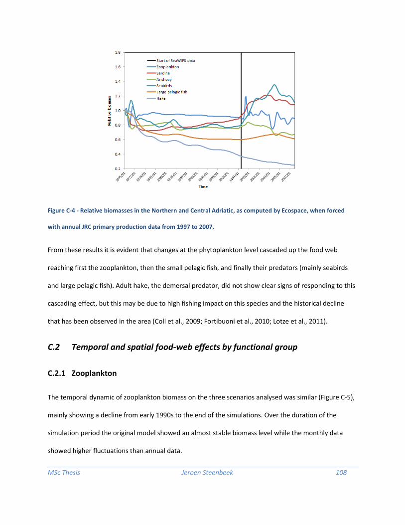
MSc Thesis Jeroen Steenbeek 108
Figure C-4 - Relative biomasses in the Northern and Central Adriatic, as computed by Ecospace, when forced
with annual JRC primary production data from 1997 to 2007.
From these results it is evident that changes at the phytoplankton level cascaded up the food web
reaching first the zooplankton, then the small pelagic fish, and finally their predators (mainly seabirds
and large pelagic fish). Adult hake, the demersal predator, did not show clear signs of responding to this
cascading effect, but this may be due to high fishing impact on this species and the historical decline
that has been observed in the area (Coll et al., 2009; Fortibuoni et al., 2010; Lotze et al., 2011).
C.2 Temporal and spatial food-web effects by functional group
C.2.1 Zooplankton
The temporal dynamic of zooplankton biomass on the three scenarios analysed was similar (Figure C-5),
mainly showing a decline from early 1990s to the end of the simulations. Over the duration of the
simulation period the original model showed an almost stable biomass level while the monthly data
showed higher fluctuations than annual data.

MSc Thesis Jeroen Steenbeek 109
The spatial dynamics of zooplankton biomass of the original model captured some of the phytoplankton
spatial dynamics (Figure C-6a), although the spatial patterns were more realistic when the external data
under the second and third scenarios were used (Figures C-6b and C-6c) showing higher zooplankton
biomass in northern and western coastal areas of the study region. Differences in spatial distributions
between the second and the third scenario were small (Figures C-6b and C-6c), showing that both
monthly and annual averaged data produced similar results at the end of the modelling runs.
Figure C-5 –Ecospace relative dynamics of zooplankton biomass, relative to the start value, for the three
scenarios analysed.

MSc Thesis Jeroen Steenbeek 110
Figure C-6 - Ecospace map showing the distribution of relative biomass of zooplankton for the last year of the
simulation, 2007. Results are related with the model (a) without external PP data, (b) with monthly PP data, and
(c) with annual PP data.
C.2.2 Sardines
The temporal dynamic of sardine biomass under the three scenarios analysed show differences (Figure
C-7) due to a decline of phytoplankton biomass in the second and third scenario that was not
reproduced in the first one (Figure 33).
The spatial dynamics of sardine biomass of the original model captured some of the phytoplankton
spatial dynamics (Figure C-8a), although the spatial patterns were also clearer when the external data
was used (Figures C-8b and C-8c). Differences between the second and the third scenario were also
small (Figures C-8b and C-8c), as for the zooplankton functional group.
b a c
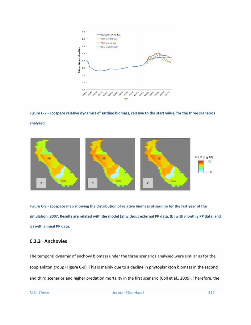
MSc Thesis Jeroen Steenbeek 111
Figure C-7 - Ecospace relative dynamics of sardine biomass, relative to the start value, for the three scenarios
analysed.
Figure C-8 - Ecospace map showing the distribution of relative biomass of sardine for the last year of the
simulation, 2007. Results are related with the model (a) without external PP data, (b) with monthly PP data, and
(c) with annual PP data.
C.2.3 Anchovies
The temporal dynamic of anchovy biomass under the three scenarios analysed were similar as for the
zooplankton group (Figure C-9). This is mainly due to a decline in phytoplankton biomass in the second
and third scenarios and higher predation mortality in the first scenario (Coll et al., 2009). Therefore, the
b a c
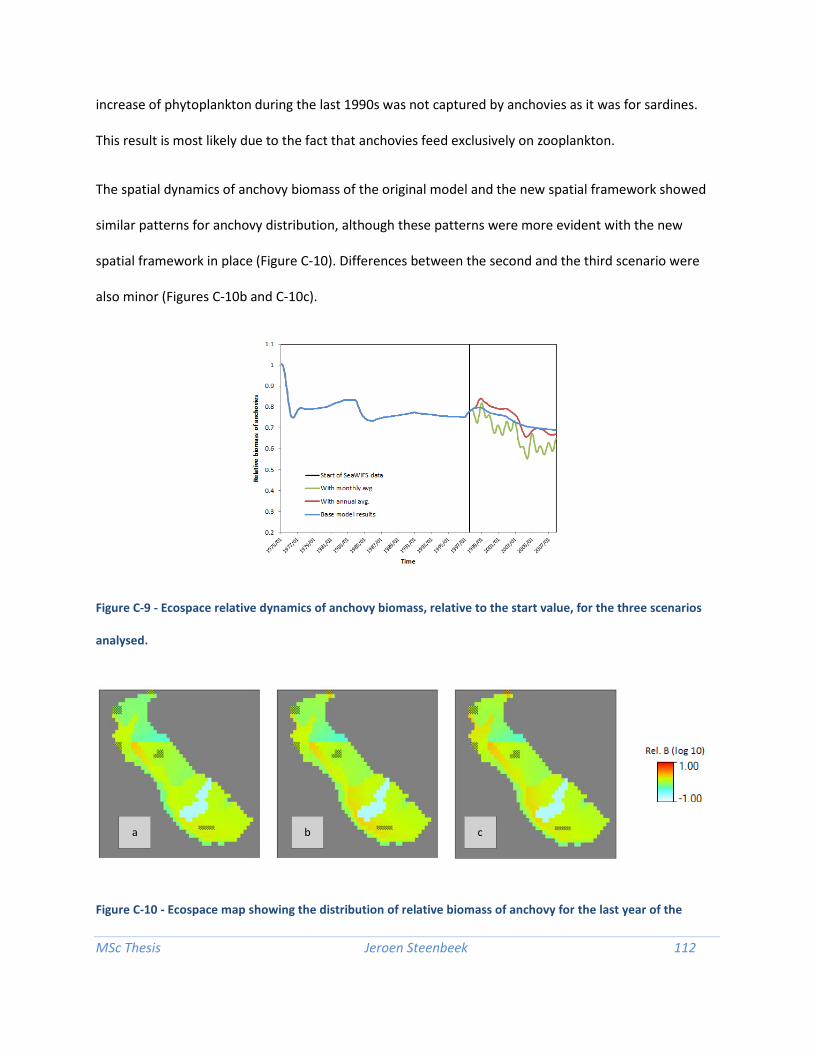
MSc Thesis Jeroen Steenbeek 112
increase of phytoplankton during the last 1990s was not captured by anchovies as it was for sardines.
This result is most likely due to the fact that anchovies feed exclusively on zooplankton.
The spatial dynamics of anchovy biomass of the original model and the new spatial framework showed
similar patterns for anchovy distribution, although these patterns were more evident with the new
spatial framework in place (Figure C-10). Differences between the second and the third scenario were
also minor (Figures C-10b and C-10c).
Figure C-9 - Ecospace relative dynamics of anchovy biomass, relative to the start value, for the three scenarios
analysed.
Figure C-10 - Ecospace map showing the distribution of relative biomass of anchovy for the last year of the
b a c

MSc Thesis Jeroen Steenbeek 113
simulation, 2007. Results are related with the model (a) without external PP data, (b) with monthly PP data, and
(c) with annual PP data.
C.2.4 Seabirds
Seabirds’ biomass also showed first an increase and then a decrease of biomass from the early 1990s to
late 2000s following sardine’s dynamics (Figure C-11) based on the second and third scenarios using the
new spatial framework. The original model, on the contrary, showed an increase and stabilization of
seabirds with time. This is due to seabirds being parameterized in the food-web model to consume
mostly sardine (Coll et al., 2009).
The spatial distribution of seabirds’ biomass was similar under the three simulations (Figures C-12a to C-
12c). However, the original model predicted less abundance of seabirds in the northern areas of the
Adriatic Sea, probably due to less productivity patterns predicted in that area (Figure 35). This is less
realistic than results using the new spatial module since seabird populations in the north of the Adriatic
Sea are known to be very abundant (e.g. Boldreghini et al., 1997).
Figure C-11 - Ecospace relative dynamics of seabirds’ biomass, relative to the start value, for the three scenarios
analysed.

MSc Thesis Jeroen Steenbeek 114
Figure C-12 - Ecospace map showing the distribution of relative biomass of seabirds for the last year of the
simulation, 2007. Results are related with the model (a) without external PP data, (b) with monthly PP data, and
(c) with annual PP data.
C.2.5 Large pelagic fish
The temporal dynamic of large pelagic fish biomass initially increased slightly and was then maintained
under the first scenario, but under the second and third scenarios this group showed a similar trend to
sardines following a similar trend to their prey (Figure C-13). However, the decline they showed under
the second and the third scenarios after the initial increase also provided evidence of their dependency
on anchovy, which declined with time (Figure C-13).
The spatial dynamics of large pelagic fish biomass of the original model and the new spatial framework
showed overall similar patterns (Figure C-14a to C-14c).
b a c

MSc Thesis Jeroen Steenbeek 115
Figure C-13 - Ecospace relative dynamics of large pelagic fish biomass, relative to the start value, for the three
scenarios analysed.
Figure C-14 - Ecospace map showing the distribution of relative biomass of large pelagic fish for the last year of
the simulation, 2007. Results are related with the model (a) without external PP data, (b) with monthly PP data,
and (c) with annual PP data.
C.2.6 Adult hake
Finally, the temporal dynamic of adult hake showed a strong declined in the three analysed scenarios
(Figure C-15), mainly due to the large historical fishing impact of this species in the area (Coll et al. 2009,
Fouzai et al. 2012) and due to the decline of one of its main preys, anchovy (Figure C-9), but also of
b a c

MSc Thesis Jeroen Steenbeek 116
sardine in the last part of the time series (Figure C-8).
The spatial dynamics of adult hake biomass of the original model and the new spatial framework
showed overall similar patterns (Figure C-16).
Figure C-15 - Ecospace relative dynamics of hake biomass, relative to the start value, for the three scenarios
analysed.
Figure C-16 - Ecospace map showing the distribution of relative biomass of hake for the last year of the
simulation, 2007. Results are related with the model (a) without external PP data, (b) with monthly PP data, and
(c) with annual PP data.
b a c

MSc Thesis Jeroen Steenbeek 117
C.3 Discussion
Overall, changes in the temporal dynamics of phytoplankton biomasses cascaded up the food web and
influenced the dynamics of zooplankton and small pelagic fish, which directly feed on phytoplankton or
zooplankton (Palomera et al., 2007). The impact on the dynamics of larger predators was also
noticeable; although such impact was mitigated by other dietary links in the food web. Seabirds and
large predatory fish showed similar patterns as their prey. When the new spatial framework was in place
(under the second and third scenarios), these groups showed first an increase, followed by a decrease in
abundance due to spatial patterns of first phytoplankton, then for zooplankton, and then small pelagic
fish. The dynamics of adult hake, on the contrary, were less affected by the bottom-up effects of the
food chain due to the high fishing pressure placed upon this highly commercial species (Coll et al., 2009;
Fouzai et al., 2012).
Simulations including the external data reproduced more realistic spatial distribution of phytoplankton
and thus yielded more accurate spatial distributions of zooplankton and small pelagic fish. The
differences between the three simulations regarding the distribution of predators were less profound
and may indicate that real predator distributions are affected by other factors than just the distribution
of their prey. Either the chosen model configuration did not include all required factors to adequately
predict predator distributions, or the biological dynamics are overshadowed by other impacts such as
high fishing pressure.
MSc Thesis Jeroen Steenbeek 118
C.4 References
Boldreghini, P., Volponi, S., Santolini, R., Cherubini, G., and Utmar, P. (1997). Recent trend of the
cormorant Phalacrocorax carbo population wintering in the Northern Adriatic, Italy. Ekologia Polska
45(1), 17–22.
Coll, M., Palomera, I., and Tudela, S. (2009). Decadal changes in a NW Mediterranean Sea food web in
relation to fishing exploitation. Ecological Modelling 220(17), 2088–2102.
Coll, M., Santojanni, A., Palomera, I., and Arneri, E. (2010). Ecosystem assessment of the North-Central
Adriatic Sea: towards a multivariate reference framework. Marine Ecology Progress Series 417, 193–210.
Coll, M., Santojanni, A., Palomera, I., Tudela, S., and Arneri, E. (2007). An ecological model of the
Northern and Central Adriatic Sea: Analysis of ecosystem structure and fishing impacts. Journal of
Marine Systems 67(1-2), 119–154.
Fortibuoni, T., Libralato, S., Raicevich, S., Giovanardi, O., and Solidoro, C. (2010). Coding early naturalists’
accounts into long-term fish community changes in the Adriatic Sea (1800–2000). PloS One 5(11),
e15502.
Fouzai, N., Coll, M., Palomera, I., Santojanni, A., Arneri, E., and Christensen, V. (2012). Fishing
management scenarios to rebuild exploited resources and ecosystems of the Northern-Central Adriatic
(Mediterranean Sea). Journal of Marine Systems 102-104, 39–51.
Lotze, H.K., Coll, M., and Dunne, J.A. (2011). Historical changes in marine resources, food-web structure
and ecosystem functioning in the Adriatic sea, Mediterranean. Ecosystems 14(2), 198–222.
Palomera, I., Olivar, M.P., Salat, J., Sabatés, A., Coll, M., García, A., and Morales-Nin, B. (2007). Small

MSc Thesis Jeroen Steenbeek 119
pelagic fish in the NW Mediterranean Sea: An ecological review. Progress In Oceanography 74(2–3),
377–396.