Branch-Cut-Price Algorithms for Solving a Class of

Search Problems on General Graphs

Z. Caner Taskın∗ J. Cole Smith†

February 21, 2017

Abstract

We consider graph search problems involving an intruder and mobile searchers. The

graph consists of nodes on which the intruder and searchers may be located, and edges

on which these entities travel. Associated with each node is a set of nodes that are

visible from that node. The goal is to find the minimum number of searchers needed to

detect the intruder within a given time limit. We investigate three variants of the graph

search problem: (i) a hide-and-seek problem, in which a stationary intruder “hides” at

an unknown node, (ii) a pursuit-evasion problem, in which the intruder moves among

the nodes to avoid being detected, and (iii) a patrol problem, which is similar to the

pursuit-evasion problem except that searchers patrol the graph in repeated circuits to

seek intruders. Our contribution provides exponential-size set-covering formulations for

these problems, along with a class of branch-cut-price algorithms tailored for solving

them. These algorithms leverage results from the orienteering literature to solve pricing

problems related to searcher routes.

∗Department of Industrial Engineering, Bogazici University, 34342 Bebek, Istanbul, Turkey; e-mail:caner.taskin@boun.edu.tr.†Department of Industrial Engineering, Clemson University, Clemson, SC 29634, USA; e-mail:

jcsmith@clemson.edu.

1

1 Introduction and Literature Review

In this paper we consider a class of graph search problems involving an intruder and a group

of searchers. Consider a graph G = (N,E) with node set N and edge set E. We assume

that G is connected and that |N | ≥ 3. Edges can either be directed or undirected, and may

contain self-loops. For simplicity in this paper, we assume that E is undirected and that

it includes self-loops for every node unless otherwise specified, although these assumptions

are not restrictive. The intruder and searchers occupy some nodes of the graph. At each

time period each player (intruder or searcher) can move along an edge to an adjacent node.

A searcher located at node i ∈ N can detect an intruder if it is located at some node

in S(i) ⊆ N , i.e., S(i) is the set of nodes that are viewable by the searchers from node

i. Searchers can be deployed at any node, but have no information about the location of

the intruder. Therefore, they must cooperatively search the graph to detect the intruder.

The problem is to find the minimum number of searchers, accompanied by the searchers’

routes, that can guarantee detection of the intruder within a given time limit, T . Because

detection must be guaranteed, we assume that the intruder has perfect information about

the searchers’ plan, and utilizes this knowledge to evade detection for as long as possible.

1.1 Problem Description and Illustration

This paper investigates three types of search problems on graphs described above. The first

is a hide-and-seek problem, in which the goal is to deploy the fewest number of searchers that

can detect a stationary intruder within some T time steps. For this case (and all examples

in this section), assume that for each i ∈ N , S(i) consists of node i and all nodes adjacent to

node i in the graph. Figure 1 shows a graph for which the optimal objective function value

is 2, given T = 1. One searcher starts at node 2 and moves to node 5 (the shaded nodes

in Figure 1), and the other searcher starts at node 7 and moves to node 8. A stationary

intruder at any node will be found by one of the searchers at either time 0 or time 1.

By contrast, in the pursuit-evasion problem, the goal is to use the fewest number of

searchers needed to identify a mobile intruder within some T time steps. The intruder can

2

1

2

3

4

5

63

7

8

93

Figure 1: Example hide-and-seek solution for T = 1

start anywhere in the graph, and at each time step, can stay at a node or move to an adjacent

node. In the example depicted by Figure 2, the time limit is T = 2. The optimal objective

function value for this problem is 2. One optimal solution starts a searcher at node 5, which

moves to node 2 at time 1 and stays at node 2 at time 2. The second searcher starts at node

7, and then moves to nodes 8 and 9 at times 1 and 2, respectively. To see that this solution

is optimal, we need to demonstrate that it is feasible, and that it is impossible to guarantee

detection with only one searcher. For feasibility, consider for each time period the set of

“safe nodes” that are not observed by the searchers:

• Time 0: Nodes 3, 9, and 10.

• Time 1: Nodes 1, 4, 6, and 10.

• Time 2: Nodes 1, 4, and 7.

There are no edges from any safe node at time 0 to nodes 1 or 4 at time 1. Hence, for an

intruder to remain undetected at time 1, the intruder has to be at node 6 or 10 at that time.

However, there are no edges from nodes 6 or 10 to the safe nodes at time 2, so any intruder

following any route on the graph will be detected by time 2. Finally, note that one searcher

is insufficient regardless of T : An intruder can indefinitely avoid the searcher on the six-node

cycle in the graph.

3

1

2

3

4

5

63

7

8

93

10

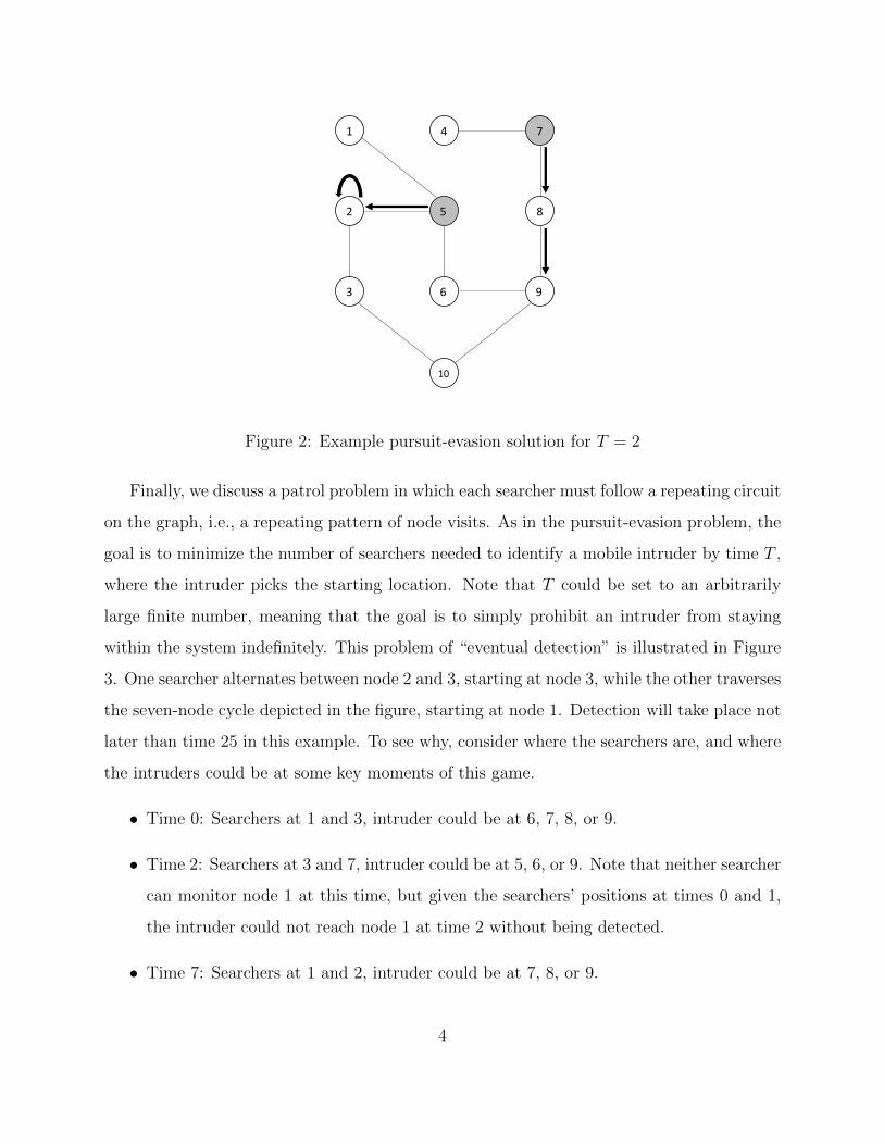
Figure 2: Example pursuit-evasion solution for T = 2

Finally, we discuss a patrol problem in which each searcher must follow a repeating circuit

on the graph, i.e., a repeating pattern of node visits. As in the pursuit-evasion problem, the

goal is to minimize the number of searchers needed to identify a mobile intruder by time T ,

where the intruder picks the starting location. Note that T could be set to an arbitrarily

large finite number, meaning that the goal is to simply prohibit an intruder from staying

within the system indefinitely. This problem of “eventual detection” is illustrated in Figure

3. One searcher alternates between node 2 and 3, starting at node 3, while the other traverses

the seven-node cycle depicted in the figure, starting at node 1. Detection will take place not

later than time 25 in this example. To see why, consider where the searchers are, and where

the intruders could be at some key moments of this game.

• Time 0: Searchers at 1 and 3, intruder could be at 6, 7, 8, or 9.

• Time 2: Searchers at 3 and 7, intruder could be at 5, 6, or 9. Note that neither searcher

can monitor node 1 at this time, but given the searchers’ positions at times 0 and 1,

the intruder could not reach node 1 at time 2 without being detected.

• Time 7: Searchers at 1 and 2, intruder could be at 7, 8, or 9.

4

• Time 14: Searchers at 1 and 3, intruder could be at 7 or 8.

• Time 21: Searchers at 1 and 2, intruder could be at 7.

After time 21, the single possible intruder location moves from 7 to 8 to 9, and finally to 6

at time 24, with the searchers positioned at nodes 3 and 8. At time 25, the searchers move

to 2 and 9, and the intruder must be identified.

1

2

3

4

5

63

7

8

93

10

Figure 3: Example patrol solution for eventual detection

In the hide-and-seek problem, the challenge is to determine searcher location and routes

to monitor the entire graph as quickly as possible. This problem motivates the use of column

generation to determine the searcher routes. By contrast, the pursuit-evasion problem not

only requires the generation of candidate searcher routes, but must also incorporate intruder

behavior. Our modeling technique will require both the dynamic generation of columns

corresponding to searcher routes and of rows corresponding to intruder routes. A similar

approach must be taken for the patrol problem, but with the added complication of looking

for searcher circuits. For the eventual-detection variation, one must now determine how an

intruder might attempt to stay undetected indefinitely. For the variation of the problem

in which detection must occur within a time limit, the intruder must determine when and

5

where to enter the graph (thus timing its entry based on the searchers’ circuits), and what

route to follow to avoid detection.

1.2 Literature Review

The graph search problem was initially defined by Parsons [32] in the context of seeking a

person lost in a cave. The cave is represented as a graph, where tunnels of the cave correspond

to graph edges. Searchers have to sweep edges of the graph to locate the missing person,

who is assumed to be wandering unpredictably or is purposefully trying to evade searchers.

The search number s(G) of a graph G is the minimum number of searchers required to find

the missing person, even if the missing person could instantly move along any path not

occupied by searchers [32]. Computing s(G) is NP-hard for general graphs [10, 28, 30], but

is computable in linear time for trees [6, 30, 33]. The search number of a graph has also been

shown to be related to the graph’s tree-width, path-width, and vertex separation [12, 14, 37].

Several variants of the graph search problem have been investigated in the literature. In

decontamination problems edges or nodes of a graph are infected by a contaminant such

as a computer virus or a chemical agent, which spreads across the graph [15, 28, 34]. In

rendezvous problems different players, who are not aware of the other players’ locations,

attempt to meet at a common node as quickly as possible [3, 5, 27].

Hide-and-seek problems consider an intruder that “hides” in a stationary location, while

the searchers try to locate the intruder in minimum time [4, 25]. Such problems also arise

in search-and-rescue settings [9]. Pursuit-evasion (or “cops-and-robber”) games model an

intruder that tries to avoid being captured by searchers [2, 7, 21, 23]. Gal [17] shows the

optimality of search strategies for specially structured graphs such as trees, and relates the

optimal search time to that required to solve the Chinese postman problem (CPP). The CPP

seeks a route that visits each edge exactly once, and starts and ends from the same node (see

the classical work of Edmonds and Johnson [13]). Relevant to our study, Jotshi and Batta

[25] examine strategies that minimize the expected time required to find a stationary hider

on a network given a single searcher. In contrast to their study, we focus on exact rather

6

than heuristic methods, and consider both the presence of multiple searchers and the case

of mobile intruders.

In other settings discussed in the literature, graph nodes need to be patrolled for protec-

tion or supervision [11, 36]. In particular, one interesting application coordinates automated

software searchers so that they patrol the Internet to find web sites that exploit browser

vulnerabilities [40]. We refer the reader to [5, 6, 16] for detailed surveys of the literature on

search problems and applications in various practical settings.

Most prior graph search research focuses on theoretical aspects of the problems (e.g.,

[11, 12, 14, 20, 37]), or on algorithms for solving the problems on special graph structures

(e.g., [4, 15, 27, 33]). Our contribution is an exact optimization algorithm for solving several

variants of the search problem on general graphs (see also [34] for a decontamination problem

in which the intruder location has been determined). We consider three specific graph search

problems: (i) a hide-and-seek problem, (ii) a pursuit-evasion problem, and (iii) a patrol

problem. We model these problems as large-scale integer programs, and propose a class

of branch-cut-price algorithms for their solution. We refer the reader to [29, 31, 35] for

foundational work on branch-and-cut algorithms, and [26] for background on branch-cut-

price theory and practice.

Because the intruder is stationary, the hide-and-seek problem is a pure optimization

problem. However, pursuit-evasion and patrol problems involve different actors whose actions

depend on the strategy used by the other actors. Thus, these problems can be seen as games

between the intruder and multiple searchers. Halvorson et al. [22] investigate a hider-seeker

game where the hider moves on a graph and the seeker, who is not constrained to move on

the graph, can observe a chosen subset of vertices in each step. They model the problem

as a two-player, zero-sum Bayesian game and find an equilibrium by using dynamic column

and row generation to solve a large-scale optimization problem. By contrast, our paper

constrains all agents to move on the graph, with a searcher at node i always observing

every vertex in S(i). Jain et al. [24] investigate a two-player Stackelberg security game

between a defender and an attacker within the context of scheduling Federal Air Marshals

7

Service agents to flights to maximize coverage. They propose a branch-and-price algorithm

in which they formulate the pricing problem as a minimum cost network flow problem. They

also introduce improved branching rules and bounds using efficient algorithms for solving

security games with relaxed scheduling constraints. Their approach is capable of solving

large-scale security games with arbitrary defender schedules. This problem is different from

the one studied in our paper in several ways: Most notably, we do not allow mixed actions by

either the searchers or the intruder, and the objective of our problem is not based on a payoff

but rather on the minimization of the number of searchers. However, the problem studied

in [24] essentially deploys searchers to patrol a network with the goal of protecting against

an intruder. On a related line of research to [24], Yang et al. [41] propose a cutting-plane

algorithm for solving Stackelberg security games with complicated adversarial models, such

as the case in which the adversary cannot make perfect decisions.

The remainder of this paper is organized as follows. In Section 2 we describe a hide-and-

seek problem and propose a branch-and-price algorithm for solving it. Similarly, Sections

3 and 4 analyze the pursuit-evasion and patrol problems, respectively, extending the prior

algorithm to a branch-cut-price framework for those problems. Section 5 provides a compar-

ison of the algorithms presented for the search problems considered in three prior sections.

We give computational results of our proposed approach in Section 6, and conclude the paper

in Section 7.

2 Hide-and-Seek Problem

We start our discussion with a hide-and-seek problem, in which a group of searchers seeks

to locate a stationary intruder within T time steps. This problem is relatively easy to model

and analyze, and serves as the basis for our more complex search algorithms. Section 2.1

gives the mathematical model for the hide-and-seek problem, and Section 2.2 describes the

proposed branch-and-price algorithm for its solution.

8

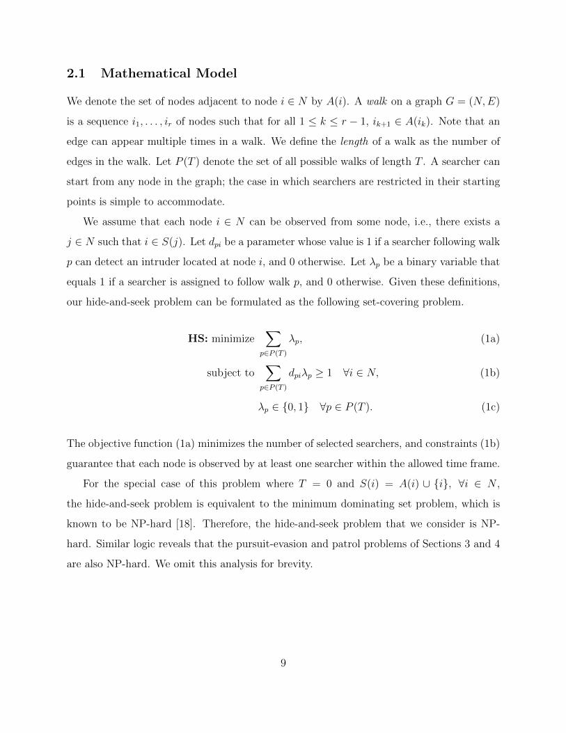
2.1 Mathematical Model

We denote the set of nodes adjacent to node i ∈ N by A(i). A walk on a graph G = (N,E)

is a sequence i1, . . . , ir of nodes such that for all 1 ≤ k ≤ r − 1, ik+1 ∈ A(ik). Note that an

edge can appear multiple times in a walk. We define the length of a walk as the number of

edges in the walk. Let P (T ) denote the set of all possible walks of length T . A searcher can

start from any node in the graph; the case in which searchers are restricted in their starting

points is simple to accommodate.

We assume that each node i ∈ N can be observed from some node, i.e., there exists a

j ∈ N such that i ∈ S(j). Let dpi be a parameter whose value is 1 if a searcher following walk

p can detect an intruder located at node i, and 0 otherwise. Let λp be a binary variable that

equals 1 if a searcher is assigned to follow walk p, and 0 otherwise. Given these definitions,

our hide-and-seek problem can be formulated as the following set-covering problem.

HS: minimize∑

p∈P (T )

λp, (1a)

subject to∑

p∈P (T )

dpiλp ≥ 1 ∀i ∈ N, (1b)

λp ∈ {0, 1} ∀p ∈ P (T ). (1c)

The objective function (1a) minimizes the number of selected searchers, and constraints (1b)

guarantee that each node is observed by at least one searcher within the allowed time frame.

For the special case of this problem where T = 0 and S(i) = A(i) ∪ {i}, ∀i ∈ N ,

the hide-and-seek problem is equivalent to the minimum dominating set problem, which is

known to be NP-hard [18]. Therefore, the hide-and-seek problem that we consider is NP-

hard. Similar logic reveals that the pursuit-evasion and patrol problems of Sections 3 and 4

are also NP-hard. We omit this analysis for brevity.

9

2.2 Solution Approach

Rather than directly solving HS, which would require the enumeration of an exponential

number of variables, we instead propose a column-generation approach to solve HS. Given

a subset of walks P ′(T ) ⊆ P (T ), we can construct a limited hide-and-seek (LHS) problem

identical to HS, with P (T ) replaced by P ′(T ). The linear programming (LP) relaxation of

LHS is:

LHS: minimize∑

p∈P ′(T )

λp, (2a)

subject to∑

p∈P ′(T )

dpiλp ≥ 1 ∀i ∈ N, (2b)

λp ≥ 0 ∀p ∈ P ′(T ), (2c)

where upper bounds on the λ-variables are not necessary at optimality. Consider a set of

optimal dual values γi associated with (2b) for i ∈ N . The reduced cost of λp, which we

denote by cp, is 1−∑

i∈N γidpi. Since γ is an optimal dual vector, cp ≥ 0 for all p ∈ P ′(T ).

An LHS solution is also optimal to the LP relaxation of HS if cp ≥ 0 for all p ∈ P (T ). On

the other hand, if cp < 0 for some p ∈ P (T ) \ P ′(T ), then adding p to P ′(T ) can potentially

decrease the value of the objective function (2a). We discuss our pricing problem, which seeks

such a p, in Section 2.2.1; present our branching scheme in Section 2.2.2; and summarize the

branch-and-price scheme in Section 2.2.3.

2.2.1 Searcher’s problem

Let yi be a decision variable that equals 1 if node i is observed by a searcher following a walk

that we generate, and 0 otherwise, ∀i ∈ N . Given an optimal dual vector γ, and recalling

that γ ≥ 0, we solve the following pricing problem to identify a λ-variable having a negative

reduced cost: max∑

i∈N γiyi, subject to the restriction that (y1, . . . , y|N |) corresponds to a

set of nodes observed by a walk of length T .

The pricing problem can be formulated as a mixed-integer programming problem on a

10

time-expanded network consisting of T + 1 stages. In particular, we create a node Nit for

each i ∈ N, t = 0, . . . , T . An arc is then generated from node Nit, ∀i ∈ N, t = 0, . . . , T − 1

to nodes Nj(t+1) for all j ∈ A(i). For the hide-and-seek problem, it is easy to see that an

optimal solution exists in which all searchers move to a different node at each time period,

and hence there is no need to create arcs between nodes Nit and Ni(t+1) for each i ∈ N .

Figure 4 displays an example graph and its corresponding time-expanded network for T = 2.

(a) (b)

Figure 4: (a) An example graph; (b) Time-expanded network for T = 2

To formulate the pricing problem as a mixed-integer program, we introduce binary vari-

ables xti = 1 if the searcher visits node i at time t. Then, an integer programming formulation

for the pricing problem can be given as:

maximize∑i∈N

γiyi, (3a)

subject to∑i∈N

xti = 1 ∀t = 0, . . . , T, (3b)

xtj ≤∑

i∈A(j)\{j}

xt−1i ∀j ∈ N, t = 1, . . . , T, (3c)

xtj ≤∑

i∈A(j)\{j}

xt+1i ∀j ∈ N, t = 0, . . . , T − 1, (3d)

yi ≤T∑t=0

∑j:i∈S(j)

xtj ∀i ∈ N, (3e)

11

0 ≤ yi ≤ 1 ∀i ∈ N, (3f)

xti ∈ {0, 1}, ∀i ∈ N, t = 0, . . . , T. (3g)

Constraints (3b) restrict the searcher to visit only one node at a time. Constraints (3c)

ensure that node j can be visited at time t only if one of its neighbors (other than j itself)

has been visited at time t − 1. Similarly, Constraints (3d) state that if node j is visited at

time t, then the next node visited at time t + 1 must be in A(j) \ {j}. (As we will state in

Remark 2, these constraints are not necessary for model correctness, but do tighten its linear

programming relaxation.) Constraints (3e) force the value of yi to equal zero unless node i

can be observed by the searcher at some time period. Note that the y-variables will take on

their correct binary values in an optimal solution, and therefore we relax them as continuous

in (3f). The x-variables are required to be binary by constraints (3g). If the optimal objective

function value of formulation (3) is greater than 1, then the λ-variable corresponding to this

solution has a negative reduced cost, and we therefore add the generated column to LHS.

To justify the next set of constraints for the hide-and-seek problem, consider a walk

p ∈ P (T ), and define its reflection p′ to be the walk resulting from reversing the order in

which nodes are visited in p. For the case in which the intruder is stationary, p and p′ are

interchangeable, in the sense that a solution containing p remains feasible when p is replaced

by p′. See [38] for a discussion of symmetry in mixed-integer programming problems, and

why the presence of symmetry impairs the solvability of such problems. In the context of

branch-and-price algorithms, removing symmetry also prevents the regeneration of columns

that are identical to those that have been eliminated in a prior step of the algorithm. We

can partially eliminate symmetry by simply requiring that the index of the starting node

in a searcher’s walk be no more than the index of the last node of the searcher’s walk. For

these problems, however, it turns out that a stronger symmetry-breaking condition can also

be stated, as given by the following proposition.

Proposition 1. Define p(k) to be the kth node visited in walk p. There exists a solution to

problem HS in which λp = 0 for every p ∈ P (T ) such that p(0) ≥ p(T ).

12

Proof. Consider any optimal solution in which λp = 1 for p ∈ P (T ) : p(0) ≥ p(T ). Note that

for any walk p ∈ P (T ) that visits all nodes visited by walk p, we have that

⋃i=0,...,T

S(p(i)) ⊆⋃

i=0,...,T

S(p(i));

therefore, an alternative optimal solution exists in which λp = 0 and λp = 1. If p(0) > p(T )

then its reflection p′ visits the same set of nodes as p. Replacing p with p′ in the HS solution,

and noting that p′(0) < p′(T ), establishes the result.

Otherwise, p(0) = p(T ), and there are two cases to consider. In case 1, p(T − 1) is not a

leaf node, and is therefore connected to some node n 6= p(0). Let walk p be given exactly as

p, except that p(T ) = n. Because p(0) = p(T ), but p does not necessarily visit node n, the

set of nodes visited by p is a subset of those visited by p. Also, p(0) 6= p(T ), so replacing p

in the HS solution with p if p(0) < p(T ), or with its reflection p′ if p(0) > p(T ), establishes

the result in this case.

In case 2, p(T − 1) is a leaf node connected to p(T ) (= p(0)). This implies by the

connectivity of G, and the assumption that |N | ≥ 3, that p(0) is not a leaf node, and is

connected to some node n 6= p(T − 1). Consider an alternative walk p that starts at node

n, and then follows walk p from time 0 to time T − 1, i.e., p(0) = n and p(i) = p(i − 1),

for i = 1, . . . , T . By the same argument as before, p visits all nodes visited by p, but

p(0) 6= p(T ). Thus, we can again replace p in the HS solution by either p (if p(0) < p(T )) or

p′ (if p(0) > p(T )). This completes the proof.

Due to Proposition 1, we include the following symmetry-breaking constraints within

formulation (3) for the hide-and-seek problem:

x0j ≤

∑i∈N :i>j

xTi ∀j ∈ N, (4)

which implies that x0|N | = xT1 = 0.

Remark 1. The pricing problem is a variation of the orienteering problem of Golden et

13

al. [19]. The orienteering problem can be defined on a graph such as the one we consider

here, along with edge lengths and nonnegative rewards that exist at nodes. The objective is

to identify a path that accumulates the maximum reward on the graph (given by the sum

of rewards at nodes visited in the path), subject to the restrictions that the sum of edge

lengths traveled in the graph is constrained by some maximum limit and that each vertex

can be visited at most once. Formulation (3) differs from other orienteering formulations

in the literature because of the following features: i) a searcher can revisit nodes during

the walk (although it only accumulates each node reward at most once), ii) a reward in

node i can be collected by a searcher that visits any node j such that i ∈ S(j), and iii)

the fact that rewards can be negative due to our branching strategy that we will discuss in

Section 2.2.2. Even though the first feature can be modeled in the orienteering problem by

introducing multiple copies of each node such that only one of the duplicates has nonzero

reward, existing algorithms for orienteering evidently cannot be directly used to solve our

pricing problem due to the existence of the other features. 2

Remark 2. Because the searcher’s walk is guaranteed to be connected due to Constraints

(3b) and (3c), Constraints (3d) can be omitted from the formulation. However, the latter

set of constraints may strengthen the linear programming relaxation of (3). Consider the

problem depicted in Figure 5, where T = 1, and suppose that γi = 1 for each i = 1, . . . , 7.

In this example, A(i) is given by the set of nodes adjacent to node i in the figure, for each

i. Also, S(i) is given by A(i) ∪ {i}, for all i. For instance, a searcher at node 4 can move

to nodes 3, 5, or 6 at the next time step, and can monitor nodes 3–6. Table 1 depicts

an optimal solution to this problem using formulation (3) without Constraints (3d). Here,

portions of the walk can disappear at some nodes and reappear at non-adjacent nodes. For

instance, 50% of a searcher exists at node 2 during time 0; however, no searcher exists at

nodes adjacent to node 2 at time 1). Constraints (3d) remove this solution from the feasible

region. The optimal solution identified by the model with constraints (3d) is given by Table

2, and has a smaller objective function value than the solution depicted in Table 1.

Next, consider the situation in which searchers are allowed to remain at their current node

14

from one time period to the next. This will be the case for the pursuit-evasion and patrol

versions of this problem. In this case, neither (3c) nor (3d) are capable of strengthening the

linear programming relaxation of (3). This is because there exists a (typically fractional)

optimal solution in which every xti = xt+1i , for every i ∈ N and j = 0, . . . , T − 1 when self-

loops exist. To see this, consider any optimal solution xti, ∀i, t, to the linear programming

relaxation of (3). Then setting xti =∑

t xti/(T + 1), ∀i, t, is a feasible solution having the

same objective function value, and must also be optimal. However, constraints (3d) can

help to strengthen the linear programming relaxation of (3) at nodes below the root of the

branch-and-bound tree, even when searchers are not required to move to different nodes

at each time period. For instance, using the same network as in Figure 5, suppose that

x11 = x1

2 = x13 = x1

4 = 0 due to branching. Without (3d), an optimal solution exists in which

0.5 searchers are located at both nodes 2 and 4 at time 0, and at nodes 5 and 6 at time 1,

yielding an objective function value of 6. (Note that the 50% searcher at node 2 “disappears”

in between the two times.) However, if Constraints (3d) are included in the model, one new

optimal solution is x04 = x1

5 = 1, with all other variables equal to zero, yielding an objective

function value of 5. 2

Figure 5: Example with T = 1 and all γi = 1, showing that Constraints (3d) are capable ofstrengthening formulation (3).

Remark 3. Let d = maxi∈N |A(i)| denote the maximum node degree in G. The total

15

Table 1: Optimal solution having objective function value 6.3 to (3) in Figure 5 without (3d)i = 1 i = 2 i = 3 i = 4 i = 5 i = 6 i = 7

x0i 0 0.5 0.1 0 0.1 0.1 0.2x1i 0 0.1 0 0.3 0.2 0.2 0.2yi 0.6 0.7 1 1 1 1 1

Table 2: Optimal solution having objective function value 6.2 to (3) in Figure 5 with (3d)i = 1 i = 2 i = 3 i = 4 i = 5 i = 6 i = 7

x0i 0.3 0 0.1 0.3 0.1 0 0.2x1i 0 0.4 0 0.2 0.1 0.2 0.1yi 0.7 0.8 1 1 1 1 0.7

number of searcher walks is bounded by |N |dT . Instead of solving Formulation (3), which

contains |N |T binary variables and O(|N |T ) constraints, it may be more efficient to solve

the searcher’s problem by an enumeration algorithm for small values of d and T .

2.2.2 Branching rules

If the optimal solution identified by solving LHS is integer feasible after the column-generation

phase, then this solution is optimal to problem HS. Otherwise, some λ-variable is fractional,

and branching is required. Choosing a branching rule that does not increase the complexity

of solving the pricing problem is essential in column-generation algorithms. When the mas-

ter problem is a set-packing or set-partitioning problem, it is possible to branch by choosing

a subset of variables X and setting x = 0, ∀x ∈ X in one branch, and x = 0, ∀x /∈ X

in the other branch. These branching constraints can be added implicitly by removing the

corresponding variables from the problem, and adjusting the pricing problem so that those

variables are never generated in future iterations. No new variables are created in this

process, and so the pricing problem structure stays the same throughout all nodes of the

branch-and-bound tree [8, 26].

However, LHS is a set-covering problem, and the approach described above is not directly

applicable. We thus propose a multi-tiered branching rule. Given a fractional solution λ, we

first calculate vi =∑

p∈P ′(T ) dpiλp, for each i ∈ N . Here, vi represents the number of times

16

that node i is observed during the search, and recall that P ′(T ) is a subset of length-T walks

that have already been generated by the algorithm. If there exists a fractional vi-value for

some i ∈ N , then we branch on vi, which represents the left-hand side of constraint (2b)

corresponding to i, as follows. In the up-branch, we simply change the right-hand-side value

of the constraint as dvre. On the down-branch, we set the upper bound of the constraint

expression to bvrc (and convert it to an equality constraint if bvrc = 1). We refer to this

scheme as constraint-based branching. Note that this scheme does not introduce new dual

variables or constraints to the pricing problems.

Under the constraint-based branching scheme, note that the dual variable γi can become

negative after branching down on the constraint (2b) corresponding to i. In this case, yi

will equal 0 at optimality in formulation (3), regardless of the x-variable values. Hence, it

becomes necessary to add constraints that force yi to 1 if the searcher’s chosen path detects

intruder i. These constraints take the form

yi ≥ xtj ∀i ∈ N, j : i ∈ S(j), t = 0, . . . , T. (5)

Next, it is possible to have a fractional solution λ for which all v-values are integral, and

therefore the branching rule described above is not always adequate. In such cases we say

that the constraint-based fails, and we instead apply a simple variable-based branching rule

as follows. For some fractional variable λp, we create two branches: one with λp = 0, and the

other with λp = 1. In the down-branch, we simply eliminate the column corresponding to λp

from the set-covering formulation. In the up-branch we need to adjust the right-hand-side

vector of our set-covering problem before eliminating λp. In either case we adjust the pricing

problems so that the same variable cannot be regenerated. Denote by W (p) the set of time-

expanded node indices corresponding to a searcher walk p. We can enforce the condition

that walk p is not generated again by adding the following constraint to the corresponding

17

searcher’s pricing problem:

∑(i,t)∈W (p)

xti ≤ |W (p)| − 1. (6)

Constraints of the form (6) are weak, since only one particular searcher walk is eliminated.

Furthermore, we observe that in our restricted master problem, columns corresponding to

two walks p and p′ would be identical if walkers following p and p′ can observe the same

set of nodes (possibly in different sequences). Thus, eliminating a particular walk p by a

constraint (6) might result in the generation of an alternative walk p′ that has the same

column of dpi values, still resulting in a fractional solution. To overcome this, one can cut

off the column of dpi values from the searcher’s pricing problem by adding:

∑i:dpi=0

yi +∑i:dpi=1

(1− yi) ≥ 1. (7)

Constraints (7) are stronger than (6), but they can be tightened further. Let N(p) denote

the set of nodes observed by a searcher following walk p. We observe that searcher walk p′

is dominated by searcher walk p if N(p′) ⊂ N(p). The following constraint indicates that

if a searcher walk p is forbidden, then no other searcher walks having N ′(p) ⊂ N(p) can

be generated (i.e., new searchers must be able to observe at least one node that cannot be

observed by p):

∑i:dpi=0

yi ≥ 1. (8)

Our variable-based branching rule changes the feasible region of the pricing problem

depending on earlier branching decisions. Hence, we only apply variable-based branching if

our constraint-based branching rule fails.

18

2.2.3 Branch-and-price algorithm

The branch-and-price algorithm we propose for the hide-and-seek problem is summarized as

follows.

• Step 0: Choose a feasible set of initial searcher walks, in which every node is seen by

at least one searcher.

• Step 1: Solve LHS, obtaining optimal solution λ and optimal dual variable values γ.

Go to Step 2.

• Step 2: Solve the column-generation problem (3). If the optimal objective function

value exceeds 1, then add the column corresponding to the solution of (3) to LHS, and

return to Step 1. Otherwise, go to Step 3.

• Step 3: If solution λ is fractional, then branch, and solve the child problems recursively.

Otherwise, terminate with λ as an optimal solution.

We initialize our algorithm in Step 0 as follows. For each node i ∈ N , we generate a stationary

searcher that stays at node i for all T periods. These searchers would not be generated in the

column-generation problem (which prohibits the searchers from being stationary), and are

less effective than searchers who remain mobile through time T . However, these stationary

searchers are sufficient to guarantee an initial feasible solution to LHS.

3 Pursuit-Evasion Problem

In this section, we consider a pursuit-evasion variant of the search problem. Unlike the

hide-and-seek problem, the intruder is also mobile in this variant, and tries to avoid the

searchers. We provide a branch-cut-price algorithm for the pursuit-evasion problem. Section

3.1 gives the mathematical model for this problem, while Sections 3.2 and 3.3 respectively

describe the column-generation and cutting-plane procedures within the algorithm. Section

3.4 summarizes the algorithm.

19

3.1 Mathematical Model

Similar to the hide-and-seek problem, we define P (T ) to be the set of all possible walks of

length T that can be taken by searchers or the intruder. Let dpr be a parameter whose value

is 1 if a searcher following walk p detects an intruder following walk r, and 0 otherwise. The

formulation for this model, which we denote by PE, is identical to that for HS, except where

(1b) is replaced by the exponential inequality set

∑p∈P (T )

dprλp ≥ 1 ∀r ∈ P (T ), (9)

where variable λp again equals 1 if and only if a searcher is assigned to follow walk p.

Constraints (9) ensure that for each possible intruder walk of length T , at least one searcher

is selected to detect it.

A static model for the pursuit-evasion problem would necessitate all possible search pat-

terns of length T , along with all evasion patterns of length T . In our branch-cut-price

algorithm, we start with a subset of search patterns P ′(T ) ⊆ P (T ) and evasion patterns

R′(T ) ⊆ P (T ), and solve a limited pursuit-evasion (LPE) problem. Problem LPE is iden-

tical to PE, except limited to searcher routes P ′(T ) and evasion patterns R′(T ). We next

describe how to generate new search and evasion patterns as needed.

3.2 Searcher’s problem

Given a subset R′(T ) of intruder walks, the searcher’s problem is similar to the pricing

problem in the hide-and-seek problem. Let γr be the dual variable associated with the

constraint of type (9) corresponding to intruder walk r ∈ R′(T ). Also, let yr be a decision

variable that equals 1 if an intruder following walk r is detected by a searcher following the

walk that we generate, and 0 otherwise, ∀r ∈ R′(T ). Given an optimal dual solution γ of the

linear programming relaxation to LPE, LPE, we solve the following pricing problem, which

is identical to model (3) with the following exceptions. One, it may be (uniquely) optimal for

a searcher to remain at the same node from one time period to the next. Hence, if a self-loop

20

exists for node i ∈ N , then an arc will exist from node Nit to Ni,t+1 in the time-expanded

pricing network, for t < T . Two, we now require a modified parameter dtir, which equals 1 if

a searcher located at node i at time t can detect an intruder following walk r, and equals 0

otherwise. Three, symmetry-breaking constraints (4) can no longer be applied, because the

intruder is no longer stationary.

The remaining details of the pricing problem remain unchanged. The revised formulation

for the pricing problem is given as follows:

maximize∑

r∈R′(T )

γryr, (10a)

subject to∑i∈N

xti = 1 ∀t = 0, . . . , T, (10b)

xtj ≤∑i∈A(j)

xt−1i ∀j ∈ N, t = 1, . . . , T, (10c)

xtj ≤∑i∈A(j)

xt+1i ∀j ∈ N, t = 0, . . . , T − 1, (10d)

yr ≤T∑t=0

∑i∈N

dtirxti ∀r ∈ R′(T ), (10e)

0 ≤ yr ≤ 1 ∀r ∈ R′(T ), (10f)

xti ∈ {0, 1}. ∀i ∈ N, t = 0, . . . , T. (10g)

Observe that the y-variables are continuous, and thus even as the number of evasion patterns

grows, the number of binary variables in this pricing problem remains constant. Alterna-

tively, the searcher’s problem can be solved by an enumeration algorithm similar to the

approach discussed in Remark 3. As before, if the optimal objective function value of model

(10) is greater than 1, then the generated variable has a negative reduced cost and is added

to LPE.

21

3.3 Intruder’s problem

Given a feasible (but possibly fractional) solution λ to LPE that states the searchers’ pro-

posed walks, we next need to determine if (9) is violated for some r ∈ P (T ) \ R′(T ). To

achieve this, we attempt to find an intruder walk that evades the searchers through time

T . To solve this problem, we generate a time-expanded network consisting of T + 1 stages,

which contains a node Nit for each i ∈ N, t = 0, . . . , T . Similar to the network generated

for the searcher’s problem, we connect each node to its neighbors and the copy of itself in

the next stage. Let xti be a binary variable that equals one if and only if the intruder visits

node i at time t, and let yp be a decision variable that equals 1 if and only if the intruder

walk that we generate is detected by searcher p. We also introduce binary parameters etpi

that equal 1 if and only if a searcher following walk p can detect an intruder located at node

i at time t. The intruder’s problem can be formulated as:

minimize∑

p∈P ′(T )

λpyp, (11a)

subject to∑i∈N

xti = 1 ∀t = 0, . . . , T, (11b)

xtj ≤∑i∈A(j)

xt−1i ∀j ∈ N, t = 1, . . . , T, (11c)

xtj ≤∑i∈A(j)

xt+1i ∀j ∈ N, t = 0, . . . , T − 1, (11d)

yp ≥ etpixti ∀p ∈ P ′(T ), i ∈ N, t = 0, . . . , T, (11e)

0 ≤ yp ≤ 1 ∀p ∈ P ′(T ), (11f)

xti ∈ {0, 1}. ∀i ∈ N, t = 0, . . . , T. (11g)

If the optimal objective function value of formulation (11) is less than 1, x-variables

having value 1 correspond to a walk r that the intruder can take to avoid detection through

time T . In this case, we add r to R′(T ), and generate the associated constraint of type (9).

We next discuss an efficient algorithm for solving the intruder’s problem when λ is an

22

integer vector. In our algorithm we generate the time-expanded network as before, and add

a dummy start node s, along with edges to Ni0, ∀i ∈ N , which correspond to the initial

intrusion at t = 0. We also connect all nodes NiT , ∀i ∈ N , to a dummy node q. We then

trace each selected searcher’s walk, and eliminate the nodes (and the corresponding arcs)

from the time-expanded network that would lead to the detection of the intruder.

After constructing the time-expanded network as described, we seek a feasible s–q path

on the network that avoids all node/time pairs that are monitored by at least one searcher.

This process is achieved by a standard breadth-first-search algorithm, which requiresO(|E|T )

computations. If such a path exists, then it corresponds to a walk r that the intruder can

take to avoid detection through time T . In this case, we add r to R′(T ), and generate the

associated constraint of type (9). On the other hand, if no such path exists, then λ is a

feasible solution to PE.

3.4 Branch-cut-price algorithm

The overall algorithm uses the same approach as that described in Section 2.2.3, except that

we use column-generation problem (10) instead of (3), we use LPE instead of LHS, Step

0 also initializes a set of evasion walks, and an additional step is needed to dynamically

generate evasion walks. For Step 0, we add one stationary intruder corresponding to each

node i ∈ N . For evasion walk generation, instead of terminating in Step 3 if λ is integer-

valued, we proceed to a new Step 4, described as follows.

• Step 4: Attempt to identify an evasion walk that will not be detected by the searchers’

routes λ, as described in Section 3.3. If such a walk exists, then add the evasion route

to LPE, and return to Step 1. Otherwise, terminate with λ as an optimal solution.

Finally, the branching mechanism is modified by branching on constraints (9) in our constraint-

based branching rule and enforcing (6) in our variable-based branching rule. We use (6) in

lieu of (8) because the order of node visits is now relevant in the pursuit-evasion problem,

and two walks that simply observe the same set of nodes at some point during their walks

can no longer be regarded as equivalent. Hence, (8) is not valid in this case.

23

4 Patrol Problem

For the patrol problems that we consider in this section, searchers are assigned to repeated

patrol circuits, which they follow indefinitely. We assume that the period of a patrol circuit

is no more than some parameter K, where K ≥ 1. Such a restriction might be due to a

capacity or range limit of the searchers, or due to desired frequency of visits to individual

nodes.

We consider two variants of the patrol problem. In the first variant the goal is to find

the minimum number of searchers needed, along with the corresponding patrol circuits, to

ensure that the intruder cannot avoid the searchers indefinitely. The goal of the second

variant is similar, except the intruder needs to be detected within T time periods after the

intrusion.

For both of these variants, we assume that the intruder is not initially in the network.

The intruder observes the searchers, learns their search patterns, and then picks a node and

time to enter the system. The intruder then tries to remain undetected in the graph for as

long as possible.

Sections 4.1 and 4.2 discuss algorithms for solving these two variants. Each section

discusses the column-generation (searcher circuit) problem, and row generation (intruder

walk) problems for these variants. The overall branch-cut-price algorithm is the same as

that described in Section 3.4 and is thus omitted.

4.1 Variant 1: Eventual Detection

We first describe two important characteristics of this variant, which we will use in deriving

a mathematical programming model.

Observation 1. Let S be the number of searchers, and suppose that searcher number s

follows a circuit of period ks, ∀s = 1, . . . , S. Define L as the least common multiple of

k1, . . . , kS. The searcher routes are cyclic with period L, in that all searchers repeat their

current positions on their routes every L time periods.

24

Lemma 1. If there exists an intruder walk that allows the intruder to stay in the graph

forever without being detected, then there exists an intruder circuit that the intruder can

follow to avoid detection indefinitely. Moreover, the period of one such circuit is kL, for

some integer k ≤ |N |.

Proof. Let L be calculated as given in Observation 1. Assume that there exists an intruder

walk p that the intruder can follow to avoid detection forever. Consider the location of

the intruder at time periods 0, L, 2L, . . . , |N |L after intrusion. Since at most |N | of these

locations can be distinct, there must be two time periods t1L and t2L at which the intruder

is located at the same node. In this case, an intruder that follows the original intruder’s

walk between t1L and t2L, for integers t1 and t2 such that 0 ≤ t1 < t2 ≤ |N |, repeatedly can

also avoid detection for an arbitrarily long duration. To obtain a repeated intruder circuit,

one can repeat the circuit established between periods t1L and t2L indefinitely after period

t2L, and can reverse the circuit back to period 0. This completes the proof.

Lemma 1 implies that it is sufficient to focus on intruder circuits having certain periods,

rather than walks of arbitrary length. This lemma also implies that we need not model

the feature that the intruder can start any time during the searchers’ circuits. Instead, the

intruder simply determines where on its desired circuit it should begin (at time zero).

Let P c(K) denote the set of all possible circuits of period no more than K that can be

taken by the searchers, and let Rc denote the set of all possible intruder circuits. Let dpr be

a parameter whose value is 1 if a searcher following circuit p detects an intruder following

circuit r, and 0 otherwise. The master problem is then given as before:

PP1: minimize∑

p∈P c(K)

λp, (12a)

subject to∑

p∈P c(K)

dprλp ≥ 1 ∀r ∈ Rc, (12b)

λp ∈ {0, 1} ∀p ∈ P c(K). (12c)

Our approach again starts with a subset of patrol routes P ′c(K) and evasion circuits R′c,

25

forming the limited patrol problem (LPP1).

4.1.1 Searcher’s problem

The searcher’s problem is similar to the foregoing pricing problems, but now must enforce

the condition that a searcher circuit is generated. Let γr be the dual variable associated

with constraints (12b) corresponding to intruder circuit r.

We solve the searcher’s problem by solving a series of integer programs. Let τ denote

the length of the current circuit under consideration. By considering different values of τ ∈

{1, . . . , K} we identify a circuit that optimizes the searcher’s problem. For each value of τ , we

generate a time-expanded network containing τ+1 layers of |N | nodes, each corresponding to

time periods as before. The first layer corresponds to the initial deployment of the searcher,

and the last layer is a dummy layer that we use to model the recurring patrol patterns.

As before, we define a binary variable xti for all i ∈ N, t = 0, . . . , τ , which equals 1 if the

searcher is located at node i at time t. We also define a parameter dtir(τ) = 1 if a searcher

that follows a period-τ circuit, located at node i at time t, will detect an intruder following

circuit r ∈ R′c. Note that if the searcher will be located at node i at time t, the searcher will

return to node i at times t+ τ , t+ 2τ , and so on. If the searcher would detect the intruder

at one or more of those times, then dtir(τ) = 1; otherwise, dtir(τ) = 0.

The column-generation integer program is formulated as in model (10) to seek an optimal

searcher circuit visiting exactly τ nodes, with the following modifications.

• Constraint (10e) contains parameters dtir(τ) instead of dtir.

• The following constraints,

x0i = xτi ∀i ∈ N, (13)

must be added to the formulation to ensure that the searcher’s walk forms a circuit.

The advantage in seeking circuits that have exactly a period of τ is that the dtir(τ)-values

become fixed parameters rather than variables when τ is pre-specified.

26

Remark 4. Note that integer programs corresponding to different values of τ can be

solved in any sequence. A good solution obtained by solving the searcher problem for one

particular value of τ can be used to prune subsequent problems for different values of τ

by bound. Therefore, we start by solving the searcher’s problem for decreasing values of

τ , since a searcher following a longer circuit is more likely to detect many intruder walks.

Next, observe that if τ ≤ K/2, then any circuits of size τ could have previously been

identified in the search for circuits of size 2τ . Therefore, τ -values are explored in the sequence

K,K − 1, . . . , bK/2c + 1. Finally, we skip any τ if we determine at a previous iteration of

the algorithm that no circuit of length τ exists in G.

4.1.2 Intruder’s problem

Given a selected subset of the searcher circuits, the intruder seeks a way of staying in the

system forever without being detected. Recall that the state of the system with respect to

the location of the searchers is cyclic, and its period is equal to the least common multiple

of the periods of searchers’ circuits, which we denote by L (Observation 1). Also, recall that

the intruder can stay in the system indefinitely if it can identify a walk that allows it to

return to its initial location at the end of a multiple of L steps (Lemma 1).

To solve the intruder’s problem, we generate a time-expanded network consisting of L

stages similar to the pursuit-evasion problem. We connect each node to the copy of itself and

its neighbors in the next stage by a directed arc. We also connect the nodes corresponding

to stage L to their neighbors in the first stage with a directed arc (modeling the fact that

the overall search pattern repeats after L periods). Finally, we trace each selected searcher’s

circuit, and remove nodes and arcs from the intruder’s network that would lead to the

detection of the intruder by the searcher.

We solve the intruder’s problem on the generated graph by seeking a directed cycle using

depth-first-search. If there is a cycle in this graph, then the intruder can stay in the system

forever without being detected by the searchers by following the route represented by the

cycle. In this case, we generate a cut of type (12b). Otherwise, the searcher cannot avoid

27

detection indefinitely.

4.2 Variant 2: Detection Within a Time Limit

For this patrol problem variant, the goal is to detect the intruder by time period T . Let

P c(K) and P (T ) be defined as before. This version of the patrol problem, PP2, is formulated

as in PP1, except that (12b) are now defined for every r ∈ P (T ). Problems LPP2 and LPP2

are the analogous limited and LP relaxation problems of PP2, respectively.

The searcher’s problem is identical to the pricing problems discussed in Section 4.1.1, but

the intruder’s problem now seeks a walk that allows it to remain in the graph undetected

through time T . Unlike the first variant, the intruder does not need to follow a circuit,

and so we must explicitly determine when in the searchers’ patrol circuits the intruder will

enter the graph. To solve the intruder’s problem, given a selected set of searcher patrols,

we generate a time-expanded network consisting of L stages, exactly as in the first patrol

problem variant. All arcs in this time-expanded network are assigned a length of 1. We then

add to this network a dummy start node s and a dummy end node q. Node s is connected

to all nodes by a directed arc having length 0, and all nodes are connected to q by a directed

arc having length 0. Finally, we trace each selected searcher’s circuit, and remove nodes

and arcs from the intruder’s network that would lead to the detection of the intruder by

a searcher. Observe that this time-expanded network allows the s–q path to start at any

time and end at any time, which captures the fact that the intruder can choose to enter the

network at a time that will allow it to remain undetected for as long as possible.

Solving the intruder’s problem on the time-expanded network requires the identification

of a longest s–q path, or of a cycle. If a cycle exists, then its length must be a multiple of

L. Otherwise, the nodes can be topologically ordered [1]. Either the detection of a cycle, or

the topological ordering if no cycle exists, can be performed in O(|E|L) computations. The

same complexity is then required to seek a longest path on the time-expanded network after

the nodes are topologically ordered.

If there is a cycle in the time-expanded network, then the intruder can stay in the system

28

forever without being detected by the searchers. Also, if this network is acyclic, but the

longest path length is greater than T , then the intruder can successfully evade the searchers

through time period T . In either case, we generate an intruder route and add a corresponding

inequality to LPP2. Otherwise, the current searcher walks are capable of detecting all walks

of length T .

5 Algorithmic Comparison

This section compares the approaches given for the three foregoing search problems, along

with the differences in the problem statements that necessitate these changes.

In the hide-and-seek problem, formulation HS is as a set-covering integer-programming

formulation having an exponential number of variables. The column-generation problem

yields searcher walks that move to a new node at every time step, and such that the initial

node visited has a smaller index than the last node visited (Proposition 1). Both restrictions

are valid because the intruder is stationary: The searchers cannot benefit from remaining at

a node for two consecutive time steps, and reversing the direction of a walk does not affect

the set of nodes observed by the searcher. The branching strategy given in Section 2.2.2 is

a two-phase approach that uses constraint-based branching where possible, and otherwise

uses variable-based branching. Also because of the intruder’s immobility, the variable-based

branching rule (6) can be strengthened to (8).

In the pursuit-evasion problem, instead of guaranteeing that all stationary intruders are

detected by a searcher walk, the problem is to ensure that all mobile intruders are detected

by a searcher walk. This difference replaces the O(|N |) set of constraints (2b) with the

exponential set of constraints (9). There are three main consequences of this modification.

One, both simplifications for the searcher’s problem that were made for the hide-and-seek

problem become invalid. It may be advantageous for the searcher to remain at the same node

over multiple time periods, and it now matters at which time step each searcher monitors a

set of nodes. Two, because there are now exponentially many constraints (9), they must be

dynamically generated by solving an intruder’s problem (see Section 3.3). Three, variable-

29

based branching must be revised to use (6) instead of (8) because of the intruder’s mobility.

For the patrol problem, the searcher’s problem is similar to that in the pursuit-evasion

problem. However, the searchers now need to patrol a repeated circuit instead of a walk, and

the length of that circuit is not known a priori. The modeling strategy that uses a dummy

layer of nodes in Section 4.1.1 accommodates this added complexity. The intruder seeks to

avoid detection forever (in the eventual detection model in Section 4.1) or through period T

(in the time-limited version in Section 4.2). In the first case, the intruder must avoid detection

on a circuit whose maximum length is determined by Lemma 1. For the second case, the

intruder needs to find a T -edge walk that avoids detection by the searchers instead. These

differences impact the time-expanded network used to identify evasion circuits or walks that

must dynamically be added to the limited master problem formulation. Branching occurs

with no modification from the pursuit-evasion problem.

6 Computational Results

We implemented the algorithms discussed in the previous sections in C++ on a Windows

Server 2008 R2 workstation with a 2.27 GHz CPU and 24 GB RAM. We used CPLEX

12.6.2 to solve the pricing problems and the linear programming relaxations of our set-

covering formulations. We implemented our algorithms for solving the intruder’s problem

using Boost Graph Library version 1.55 [39]. Our base set of test instances consists of 60

randomly generated instances for which the expected edge density of the graph (measured as

|E|/(|N | × (|N | − 1)), where we do not consider self-loop edges in calculating edge density)

is 10%, and the number of nodes |N | ranges from 5 to 60. In generating instances we

first picked a random subset of edges so that the edge density is 10%, added the minimum

number of edges needed to make the graph connected (see [39]), along with self-loop edges.

We generated five instances for each problem size, which is determined by the number of

nodes. Finally, we solved each instance with different values of T ∈ {1, . . . , 5} for the hide-

and-seek, pursuit-evasion and patrol problems. In each case, we assume that a searcher

located at node i ∈ N can observe node i and all nodes adjacent to it, and hence we set

30

S(i) = A(i)∪{i}, for all i ∈ N . We imposed a 1800-second time limit past which we stopped

the execution of an algorithm in all our experiments.

Further, it is useful to warm-start our procedures with an upper bound on the optimal

objective function value. Recall that all problems that we consider in this paper reduce to

the minimum dominating set (DS) problem for T = 0. If we place a stationary searcher

at every node that belongs to a feasible DS solution, the resulting solution is feasible to all

of the problem variants discussed here. Hence, we solve the DS problem before beginning

our branch-cut-price procedures to obtain an initial upper bound. (The DS formulation

is equivalent to the HS formulation with T = 0. Because |P (0)| = |N |, we simply solve

the full formulation (1) directly using CPLEX without employing any column-generation

techniques.) More sophisticated heuristics that guarantee feasible solutions can also be used

for this purpose. However, our computational experiments showed that the best upper bound

is found within one minute of CPU time for over 90% of problem instances in our base set

of test instances.

Our first experiment focuses on the hide-and-seek problem. Our preliminary compu-

tational study showed that valid inequalities (3d) and symmetry breaking constraints (4)

improve performance of our branch-and-price algorithm described in Section 2.2.3. This is

not surprising since solving the searcher’s problem (3), which is a MIP, constitutes the bot-

tleneck operation in our branch-and-price algorithm for solving the hide-and-seek problem.

Therefore, improving solvability of the searcher’s problem improves the overall algorithm’s

performance. To this end, we also implemented an enumeration algorithm to solve the

searcher’s problem. As discussed in Remark 3, the enumeration algorithm can be more ef-

ficient than solving (3) for small values of d and T . Our preliminary computational study

showed that running both the enumeration algorithm and formulation (3) to generate the

first five searchers, and then generating the rest using only the faster method, yields the best

results. Table 3 shows the results of our first experiment, where |N | denotes the number

of nodes in the graph, “Solved” denotes the number of instances that have been solved to

optimality within the given time limit, “Gap” denotes average optimality gap (calculated

31

as (upper bound − lower bound)/upper bound) and “Time” denotes the average CPU time

spent by our algorithm. Since we generated five random graphs for each value of |N | and ex-

ecuted our algorithms for different values of T ∈ {1, . . . , 5}, each line on Table 3 corresponds

to 25 instances.

Table 3: Performance of our branch-and-price algorithm for the hide-and-seek problem

|N | Solved Gap Time

5 25 0.0% 0.110 25 0.0% 0.115 25 0.0% 0.220 25 0.0% 0.425 25 0.0% 1.230 25 0.0% 5.735 25 0.0% 7.840 25 0.0% 11.345 25 0.0% 259.150 20 8.0% 462.755 20 10.7% 485.860 8 39.1% 1391.4

Table 3 shows that our branch-and-price algorithm solves all instances to optimality for

graphs having up to 45 nodes within an average of 31.8 seconds. As the number of nodes

increases, the number of instances solved to optimality within 1800 seconds decreases, and

optimality gap and CPU times increase. Note that if a problem does not solve within the

1800-second limit, we count its processing time to be 1800 seconds.

Our next experiment aims to investigate the performance of our branch-cut-price algo-

rithms for solving the pursuit-evasion problem, patrol problem variant 1 (eventual detection),

and patrol problem variant 2 (detection within a time limit). Since these problems are more

difficult to solve than the hide-and-seek problem, we limited our experiment to instances

containing at most 25 nodes. Our preliminary computational study showed that solving the

intruder’s problem by formulation (11) for fractional λ vectors is not justified computation-

ally. Thus, we solve the intruder’s problem only for integral λ vectors using our efficient

algorithm proposed in Section 3.3 for the pursuit-evasion problem.

32

Table 4: Performance of our branch-cut-price algorithms for the pursuit evasion and patrolproblems

Pursuit-Evasion Patrol Variant 1 Patrol Variant 2

|N | Solved Gap Time Solved Gap Time Solved Gap Time

5 25 0.0% 0.1 25 0.0% 0.1 25 0.0% 0.110 25 0.0% 0.2 25 0.0% 0.3 25 0.0% 0.715 25 0.0% 41.2 15 13.0% 1017.8 6 36.2% 1371.020 14 22.7% 903.4 5 23.1% 1800.0 4 42.6% 1645.325 8 37.3% 1294.1 0 37.4% 1800.0 1 45.5% 1764.6

Table 4 shows that performance of our algorithms degrade as the number of nodes in-

crease, which is not surprising since the problem’s difficulty increases with increasing |N |.

A comparison of Tables 3 and 4 reveals that our algorithm for solving the hide-and-seek

problem can solve all instances in Table 4 within a few seconds, whereas our algorithms for

solving pursuit-evasion and patrol problems can only solve a small number of 25-node in-

stances to optimality within 1800 seconds. We note that processing each branch-and-bound

node in the pursuit-evasion problem takes longer than the hide-and-seek problem due to the

fact that the intruder’s problem described in Section 3.3 is not needed for the hide-and-seek

problem. Hence, our algorithm for solving pursuit-evasion problem can process fewer nodes

within the time limit. Furthermore, Table 4 reveals that our algorithms for patrol problem

variants can solve fewer instances in our data set within the time limit compared to our

algorithms for hide-and-seek and pursuit-evasion problems. This can be explained by: (i)

our assumption that the intruder can pick a time and node to enter the system, and (ii) the

difficulty of solving the searcher’s problem for our patrol problems, which requires solving

multiple mixed-integer programs. The first factor makes it easier for the intruder to evade

the searchers, while the second factor makes the searcher’s problem more difficult to solve.

The combined effect of these factors is that processing each node takes significantly longer

than the other problems. Table 4 also shows that solving detection within a time limit vari-

ant of the patrol problem (Variant 2) requires more computational effort than the eventual

detection variant (Variant 1), which can be explained by noting that searchers have to cover

33

more intruder routes in Variant 2. (Note that any intruder circuit for Variant 1 corresponds

to an intruder route for Variant 2, but the converse is not necessarily true.)

In our next experiment we investigate the impact of allowed search time (T ) on the

number of searchers needed. Table 5 displays the average number of searchers needed for

different values of |N | and T for the hide-and-seek and pursuit-evasion problems. Each value

is an average of five instances, where we use best known solutions for instances that could

not be solved to optimality within the time limit. Note that the T = 0 column corresponds

to the cardinality of the minimum dominating set. The columns corresponding to the hide-

and-seek problem in Table 5 reveal that the minimum required number of searchers increases

as the graph gets larger, and decreases as the maximum allowed time to detect the intruder

increases. A comparison of our results for the hide-and-seek and pursuit-evasion problems

in Table 5 shows that the number of searchers needed for the hide-and-seek problem is no

more than that for the pursuit-evasion problem for a given value of T . This result is not

surprising since the intruder is stationary in the former problem, whereas it can move to

avoid the searchers in the latter one.

Table 5: Average number of searchers needed for hide-and-seek and pursuit-evasion problems

Hide-and-Seek Pursuit-Evasion

T -values: T -values:|N | T = 0 1 2 3 4 5 1 2 3 4 5

5 2 1.6 1 1 1 1 1.6 1 1 1 110 3.8 2.8 2 2 1.6 1.2 3 2.2 2 2 215 4.6 2.8 2 2 1.8 1.4 3.2 2.8 2.6 2.2 220 4.8 3.2 2 2 1.8 1.4 3.6 3 3.4 4 4.825 5.4 3 2 2 2 1.8 4 3.6 5.4 5.4 5.4

Table 6 shows the average number of searchers needed for patrol problems. Note that in

Variant 1 (eventual detection), the detection deadline T = ∞, while finite values of T are

employed for Variant 2 (detection within a time limit).

As expected, both variants of the patrol problem require fewer searchers than the dom-

inating set size (when T = 0), which reflects the case in which all nodes are continuously

34

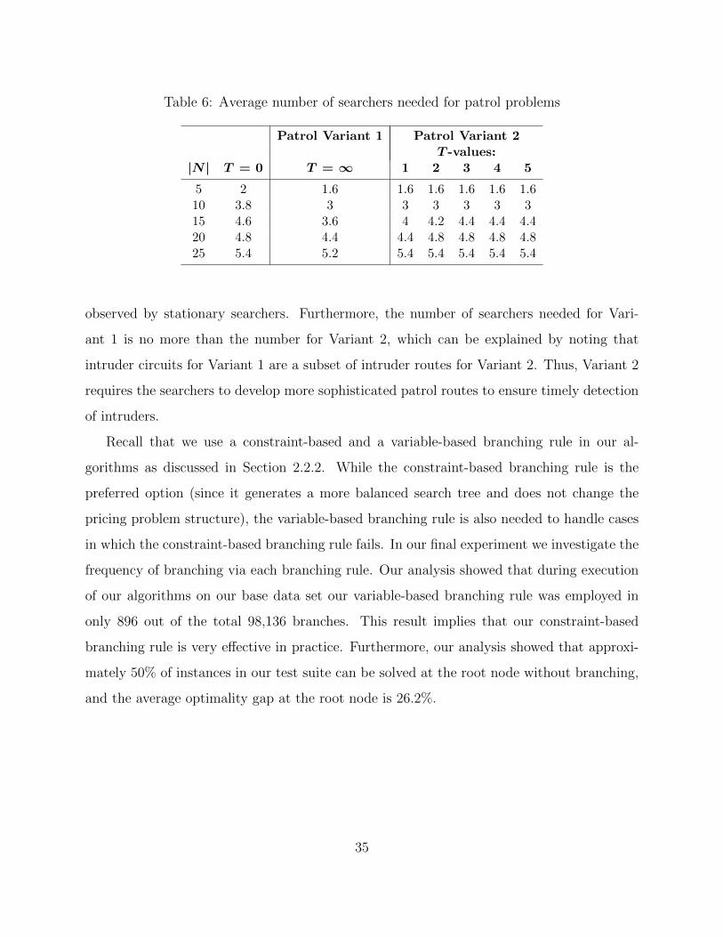
Table 6: Average number of searchers needed for patrol problems

Patrol Variant 1 Patrol Variant 2T -values:

|N | T = 0 T = ∞ 1 2 3 4 5

5 2 1.6 1.6 1.6 1.6 1.6 1.610 3.8 3 3 3 3 3 315 4.6 3.6 4 4.2 4.4 4.4 4.420 4.8 4.4 4.4 4.8 4.8 4.8 4.825 5.4 5.2 5.4 5.4 5.4 5.4 5.4

observed by stationary searchers. Furthermore, the number of searchers needed for Vari-

ant 1 is no more than the number for Variant 2, which can be explained by noting that

intruder circuits for Variant 1 are a subset of intruder routes for Variant 2. Thus, Variant 2

requires the searchers to develop more sophisticated patrol routes to ensure timely detection

of intruders.

Recall that we use a constraint-based and a variable-based branching rule in our al-

gorithms as discussed in Section 2.2.2. While the constraint-based branching rule is the

preferred option (since it generates a more balanced search tree and does not change the

pricing problem structure), the variable-based branching rule is also needed to handle cases

in which the constraint-based branching rule fails. In our final experiment we investigate the

frequency of branching via each branching rule. Our analysis showed that during execution

of our algorithms on our base data set our variable-based branching rule was employed in

only 896 out of the total 98,136 branches. This result implies that our constraint-based

branching rule is very effective in practice. Furthermore, our analysis showed that approxi-

mately 50% of instances in our test suite can be solved at the root node without branching,

and the average optimality gap at the root node is 26.2%.

35

7 Conclusions

This paper models a class of graph search problems as large-scale set-covering problems

having an exponential number of variables, and in all but one case, an exponential number

of constraints. The paper contributes specialized column-generation, row-generation, and

branching rules for these problems, and discusses the role that symmetry-breaking and valid-

inequality constraint generation play in reducing the computational effort required to solve

the problems. Our computational results show that modest-sized problems can be solved

to optimality using the proposed approach, although the instances become very difficult to

solve for the pursuit-evasion and patrol problems.

The hide-and-seek, pursuit evasion, and patrol problems that we consider are NP-hard on

general graphs. A possible future research direction is to investigate these problems on special

graphs and identify structural properties of optimal solutions. These observations could lead

to polynomial-time algorithms on specially-structured graphs. For instance, one can consider

a line graph having |N | nodes and assume that searchers can detect the intruder if it is located

at the same node or is adjacent to a searcher. In this case, an optimal solution to the hide-

and-seek and pursuit evasion problems that ensures detection of the intruder within T time

periods can be optimized as follows (where for simplicity in exposition, |N | >> T ). One

searcher starts search at node 2 and moves to node T + 2, covering nodes 1 through T + 3.

A second searcher starts at node 2T + 5 and moves to T + 5, covering nodes T + 4 through

2T + 6. A third searcher starts at node 2T + 8 and moves to 3T + 8, covering nodes 2T + 7

through 3T + 9. Splitting the graph into regions of size T + 3, the total number of searchers

needed is d|N |/(T + 3)e.

It is easy to imagine a broad array of additional search problem variations. For in-

stance, the searchers may be operating at different speeds relative to the intruder. Multiple

intruders may exist, which, if forced to take different routes, may inspire problems of min-

imizing time to find the first intruder or the average time to find all intruders. However,

given the difficulty of solving the instances posed in this paper, it may be more prudent

to develop tighter bounding mechanisms for the hide-and-seek, pursuit-evasion, and patrol

36

problems problems first. These bounds can come from heuristic strategies, or from optimal

solutions to relaxations or restrictions of the problem. An elementary example of the re-

laxation/restriction strategy arises when we (optimally) solve DS as a restriction to every

problem variant discussed in this paper in order to find an upper bound. Lower bounds may

perhaps be obtained by analogous means. For instance, in the HS problem, we could imagine

that the searchers immediately gain knowledge of the intruder’s location j after time 0, and

then take a shortest path to some node i: j ∈ S(i). This knowledge of the intruder’s location

constitutes a relaxation of the HS problem. Under this assumption, a lower bound can be

derived by solving a DS instance in which a searcher initially located at node k is assumed to

simultaneously occupy all nodes i such that the shortest-path distance (measured in terms

of the number of links) from k to i does not exceed T . However, this bound is likely to be

weak, and future research should be dedicated to exploring tighter bounding algorithms for

the problems investigated here.

Acknowledgments

The authors sincerely thank an anonymous associate editor and two anonymous referees for

their helpful and very insightful comments. This research was supported by the Defense

Threat Reduction Agency under grant HDTRA-10-01-0050, the Air Force Office of Scien-

tific Research under grant FA9550-12-1-0353, and the Office of Naval Research under grant

N000141310036.

References

[1] R. K. Ahuja, T. L. Magnanti, and J. B. Orlin. Network Flows: Theory, Algorithms,

and Applications. Prentice Hall, Upper Saddle River, NJ, 1993.

[2] M. Aigner and M. Fromme. A game of cops and robbers. Discrete Applied Mathematics,

8(1):1–12, 1984.

37

[3] S. Alpern. The rendezvous search problem. SIAM Journal on Control and Optimization,

33(3):673–683, 1995.

[4] S. Alpern. Hide-and-seek games on a tree to which Eulerian networks are attached.

Networks, 52(3):162–166, 2008.

[5] S. Alpern and S. Gal. The Theory of Search Games and Rendezvous, volume 55 of

International Series in Operations Research & Management Science. Kluwer Academic

Publishers, Dordrecht, The Netherlands, 2003.

[6] B. Alspach. Searching and sweeping graphs: a brief survey. Le Matematiche, 59:5–37,

2004.

[7] B. Alspach, D. Dyer, D. Hanson, and B. Yang. Time constrained graph searching.

Theoretical Computer Science, 399(3):158–168, 2008.

[8] C. Barnhart, E. L. Johnson, G. L. Nemhauser, M. W. P. Savelsbergh, and P. H. Vance.

Branch-and-price: Column generation for solving huge integer programs. Operations

Research, 46(3):316–329, 1998.

[9] S. J. Benkoski, M. Monticino, and J. R. Weisinger. A survey of the search theory

literature. Naval Research Logistics, 38:469–494, 1991.

[10] D. Bienstock and P. Seymour. Monotonicity in graph searching. Journal of Algorithms,

12(2):239–245, 1991.

[11] Y. Chevaleyre, F. Sempe, and G. Ramalho. A theoretical analysis of multi-agent pa-

trolling strategies. In AAMAS ’04: Proceedings of the Third International Joint Con-

ference on Autonomous Agents and Multiagent Systems, pages 1524–1525, Washington,

DC, USA, 2004. IEEE Computer Society.

[12] N. D. Dendris, L. M. Kirousis, and D. M. Thilikos. Fugitive-search games on graphs

and related parameters. Theoretical Computer Science, 172(1-2):233–254, 1997.

38

[13] J. Edmonds and E. L. Johnson. Matching Euler tours and the Chinese postman problem.

Mathematical Programming, 5(1):88–124, 1973.

[14] J. A. Ellis, I. H. Sudborough, and J. S. Turner. The vertex separation and search

number of a graph. Information and Computation, 113(1):50–79, 1994.

[15] P. Flocchini, M. J. Huang, and F. L. Luccio. Decontamination of hypercubes by mobile

agents. Networks, 52(3):167–178, 2008.

[16] F. V. Fomin and D. M. Thilikos. An annotated bibliography on guaranteed graph

searching. Theoretical Computer Science, 399(3):236–245, 2008.

[17] S. Gal. On the optimality of a simple search strategy for searching graphs. International

Journal of Game Theory, 29(4):533–542, 2000.

[18] M. R. Garey and D. S. Johnson. Computers and Intractability; A Guide to the Theory

of NP-Completeness. W. H. Freeman & Co., San Francisco, CA, 1979.

[19] B. L. Golden, L. Levy, and R. Vohra. The orienteering problem. Naval Research

Logistics, 34(3):307–318, 1987.

[20] A. S. Goldstein and E. M. Reingold. The complexity of pursuit on a graph. Theoretical

Computer Science, 143(1):93–112, 1995.

[21] G. Hahn. Cops, robbers and graphs. Tatra Mountains Mathematical Publications, 36:1–

14, 2007.

[22] E. Halvorson, V. Conitzer, and R. Parr. Multi-step multi-sensor hider-seeker games. In

Proceedings of the 21st International Joint Conference on Artificial Intelligence (IJCAI),

pages 336–341, Pasadena, CA, 2009.

[23] V. Isler and N. Karnad. The role of information in the cop-robber game. Theoretical

Computer Science, 399(3):179–190, 2008.

39

[24] M. Jain, E. Kardes, C. Kiekintveld, F. Ordonez, and M. Tambe. Security games with

arbitrary schedules: A branch and price approach. In Proceedings of the 24th AAAI

Conference on Artificial Intelligence (AAAI), 2010.

[25] A. Jotshi and R. Batta. Search for an immobile entity on a network. European Journal

of Operational Research, 191(2):347–359, 2008.

[26] M. Junger and S. Thienel. The ABACUS system for branch-and-cut-and-price algo-

rithms in integer programming and combinatorial optimization. Software Practice and

Experience, 30(11):1325–1352, 2000.

[27] K. Kikuta and W. H. Ruckle. Rendezvous search on a star graph with examination

costs. European Journal of Operational Research, 181(1):298–304, 2007.

[28] A. S. LaPaugh. Recontamination does not help to search a graph. Journal of the ACM,

40(2):224–245, 1993.

[29] H. Marchand, A. Martin, R. Weismantel, and L. Wolsey. Cutting planes in integer and

mixed integer programming. Discrete Applied Mathematics, 123(1-3):397–446, 2002.

[30] N. Megiddo, S. L. Hakimi, M. R. Garey, D. S. Johnson, and C. H. Papadimitriou. The

complexity of searching a graph. Journal of the ACM, 35(1):18–44, 1988.

[31] G. L. Nemhauser and L. A. Wolsey. Integer and Combinatorial Optimization. Wiley-

Interscience, New York, NY, 1988.

[32] T. D. Parsons. Pursuit-evasion in a graph. In Theory and Applications of Graphs, pages

426–441. Springer, Berlin, 1978.

[33] S.-L. Peng, C.-W. Ho, T.-S. Hsu, M.-T. Ko, and C. Y. Tang. Edge and node searching

problems on trees. Theoretical Computer Science, 240(2):429–446, 2000.

[34] J. Penuel, J. C. Smith, and S. Shen. Models and complexity analysis for the graph

decontamination problem with mobile agents. Networks, 61(1):1–19, 2013.

40

[35] T. K. Ralphs, L. Ladanyi, and M. J. Saltzman. Parallel branch, cut, and price for

large-scale discrete optimization. Mathematical Programming, 98(1–3):253–280, 2003.

[36] T. Sak, J. Wainer, and S. K. Goldenstein. Probabilistic multiagent patrolling. In

Advances in Artificial Intelligence – SBIA 2008. Springer, 2008.

[37] P. Seymour and R. Thomas. Graph searching and a min-max theorem for tree-width.

Jounal of Combinatorial Theory, Series B, 58(1):22–33, 1993.

[38] H. D. Sherali and J. C. Smith. Improving zero-one model representations via symmetry

considerations. Management Science, 47(10):1396–1407, 2001.

[39] J. G. Siek, L. Lee, and A. Lumsdaine. The Boost Graph Library: User Guide and

Reference Manual. Addison-Wesley, 2001.

[40] Y.-M. Wang, D. Beck, X. Jiang, and R. Roussev. Automated web patrol with strider

honeymonkeys: Finding web sites that exploit browser vulnerabilities. Technical report,

Microsoft Research, 2005.

[41] R. Yang, A. X. Jiang, F. Ordonez, and M. Tambe. Scaling-up security games with

boundedly rational adversaries: A cutting-plane approach. In Proceedings of the 23rd

International Joint Conference on Artificial Intelligence (IJCAI), pages 404–410, Bei-

jing, 2013.

41