Embed Size (px)
Citation preview
METAHEURISTIC ALGORITHMS FOR SOLVING LOT-SIZING AND SCHEDULING PROBLEMS IN SINGLE AND
MULTI-PLANT ENVIRONMENTS
MARYAM MOHAMMADI
FACULTY OF ENGINEERING UNIVERSITY OF MALAYA
KUALA LUMPUR
2015
METAHEURISTIC ALGORITHMS FOR SOLVING LOT-SIZING AND SCHEDULING PROBLEMS IN SINGLE
AND MULTI-PLANT ENVIRONMENTS
MARYAM MOHAMMADI
THESIS SUBMITTED IN FULFILMENT OF THE
REQUIREMENTS FOR THE DEGREE OF DOCTOR OF PHILOSOPHY
FACULTY OF ENGINEERING UNIVERSITY OF MALAYA
KUALA LUMPUR
2015

UNIVERSITY OF MALAYA
ORIGINAL LITERARY WORK DECLARATION
Name of Candidate: Maryam Mohammadi I.C/Passport No: I95756000
Registration/Matric No: KHA120059
Name of Degree: Doctor of Philosophy
Title of Thesis:
Metaheuristic Algorithms for Solving Lot-Sizing and Scheduling Problems in
Single and Multi-Plant Environments
Field of Study: Manufacturing Systems (Engineering and Engineering Trades)
I do solemnly and sincerely declare that:
(1) I am the sole author/writer of this Work; (2) This Work is original; (3) Any use of any work in which copyright exists was done by way of fair dealing
and for permitted purposes and any excerpt or extract from, or reference to or reproduction of any copyright work has been disclosed expressly and sufficiently and the title of the Work and its authorship have been acknowledged in this Work;
(4) I do not have any actual knowledge nor do I ought reasonably to know that the making of this work constitutes an infringement of any copyright work;
(5) I hereby assign all and every rights in the copyright to this Work to the University of Malaya (“UM”), who henceforth shall be owner of the copyright in this Work and that any reproduction or use in any form or by any means whatsoever is prohibited without the written consent of UM having been first had and obtained;
(6) I am fully aware that if in the course of making this Work I have infringed any copyright whether intentionally or otherwise, I may be subject to legal action or any other action as may be determined by UM.
Candidate’s Signature Date: 23/09/2015
Maryam Mohammadi
Subscribed and solemnly declared before,
Witness’s Signature Date: 23/09/2015
Name:
Designation:
ii
ABSTRACT
Economic lot scheduling problem (ELSP) is related to lot-sizing and scheduling several
items in a single production facility. This project addresses the ELSP where multiple
items have shelf life restrictions and planned backorders. For some products, shelf life
might be less than the production cycle time, which leads to product spoilage before the
end of the cycle. In order to achieve a feasible schedule, the production cycle time needs
to be reduced to less than or equal to the shelf life duration. While the cost-
minimization cycle time causes the spoilage of products, due to shelf life restrictions,
appropriate decisions can be made based on one of three options: production rate
reduction, cycle time reduction, or the simultaneous production rate and cycle time
reduction. For each option, the optimal cycle time and production rate are appraised,
which satisfy the shelf life constraints. On the other hand, backorders incur shelf life
constraint alteration, which affects the corresponding inventory models. Accordingly,
appropriate modifications are applied to the related mathematical inventory models.
Further, a mixed integer non-linear model for the ELSP is developed which allows each
product to be produced more than once per cycle. However, production of each item
more than one time may result in an infeasible schedule due to the overlapping
production times of various items. To eliminate the production time conflicts,
adjustments must be made through advancing or delaying the production start time of
some or all the items. The objective is to find the optimal production rate, lot size,
production frequency, cycle time, as well as a feasible manufacturing schedule for the
family of items, in addition to minimizing the total cost including production, setup,
holding, backordering, and adjustment costs.
Lot-sizing problems are more complicated in multi-facility systems because of
interdependency between facilities. Therefore, the multi-item multi-period capacitated
lot-sizing problem in a multi-stage system composed of multiple suppliers, plants, and
iii
distribution centers is addressed in order to investigate the effectiveness of coordinating
production and distribution planning. Combinations of several functions such as
purchasing, production, storage, backordering, and transportation between suppliers,
plants and distribution centers are considered. The objective is to simultaneously
determine the optimal raw material order quantity, production and inventory levels, and
the transportation amount so that the demand can be satisfied with the lowest possible
cost over a given planning horizon without violating the capacity restrictions of the
plants and suppliers. Transfer decisions between plants are made when demand
observed at a plant can be satisfied by other production sites to cope with under-
capacity of a given plant. Furthermore, the model also allows for sales at distribution
centers.
Numerical examples are presented to illustrate the effectiveness and efficiency of the
proposed models. Metaheuristic approaches namely genetic algorithm, particle swarm
optimization, artificial bee colony, simulated annealing, and imperialist competitive
algorithm are adopted for the optimization procedures. To offer more efficiency,
Taguchi method is utilized to calibrate the various parameters of the proposed
algorithms. The statistical optimization results show the efficiency, effectiveness and
robustness of the applied methods in solving the proposed optimization models.
iv
ABSTRAK
Masalah penjadualan lot ekonomi (ELSP) adalah berkait rapat dengan pensaizan lot dan
penjadualan beberapa item di dalam sebuah fasiliti pengeluaran tunggal. Projek ini
menangani ELSP yang mempunyai beberapa item dengan batasan jangka hayat dan
tunggakan tempahan terancang. Bagi sesetengah produk, jangka hayatnya mungkin
kurang daripada tempoh kitaran pengeluarannya, menyebabkan kepada kerosakan
produk sebelum tiba ke pengakhiran kitaran. Untuk mencapai penjadualan yang boleh
dilaksanakan, tempoh kitaran pengeluaran perlu dikurangkan kepada kurang daripada
atau sama dengan tempoh jangka hayatnya. Sementara tempoh kitaran dengan kos yang
diminimakan menyebabkan kerosakan produk-produk, dengan melihat kepada batasan
jangka hayat, keputusan yang sesuai boleh dibuat berdasarkan tiga pilihan: pengurangan
kadar pengeluaran, pengurangan tempoh kitaran, atau pengurangan kedua-duanya
sekali. Bagi setiap pilihan, tempoh kitaran optimum dan kadar pengeluaran dinilai,
yang mana ianya memenuhi batasan jangka hayat. Sementara itu, tempahan tertunggak
mendorong perubahan kepada batasan jangka hayat, yang kemudiannya memberikan
kesan kepada model inventorinya. Oleh itu, pengubahsuaian yang sewajarnya dibuat
kepada model inventori matematik yang berkaitan.
Seterusnya, satu model integer campuran yang bersifat tidak linear bagi ELSP
dibangunkan untuk membolehkan setiap produk dapat dihasilkan lebih daripada sekali
bagi setiap kitaran. Walaubagaimanapun, pengeluaran setiap item lebih daripada sekali
memungkinkan penjadualan yang tidak dapat dilaksanakan disebabkan adanya
pertindihan tempoh pengeluaran pelbagai item. Untuk menyingkirkan percanggahan
tempoh pengeluaran, pelarasan hendaklah dibuat dengan cara mempercepatkan atau
melambatkan masa permulaan bagi pengeluaran bagi sebahagian item atau kesemuanya
sekali. Objektifnya adalah untuk mengoptimumkan kadar pengeluaran, saiz lot,
kekerapan pengeluaran, tempoh kitaran serta penjadualan pembuatan yang dapat
v
dilaksanakan bagi kelompok item-item, di samping meminimakan kos keseluruhan
termasuk kos-kos pengeluaran, persediaan, induk, tempahan tertunggak dan kos
pelarasan.
Masalah pensaizan lot adalah lebih rumit bagi sistem dengan pelbagai fasiliti
disebabkan oleh pergantungan antara fasiliti-fasiliti tersebut. Oleh itu, permasalahan
pensaizan lot dengan kapasiti pelbagai item dan pelbagai tempoh yang merangkumi
pelbagai pembekal, loji dan pusat pengedaran diambil perhatian untuk mengkaji
keberkesanan koordinasi pengeluaran dan rancangan pengedaran. Kombinasi pelbagai
fungsi seperti pembelian, pengeluaran, penstoran, tempahan tertunggak dan
pengangkutan di antara pembekal, loji dan pusat pengedaran diambil kira. Tujuannya
adalah untuk menentukan jumlah tempahan bahan mentah yang optimum, tahapan
pengeluaran, tahapan inventori, dan jumlah pengangkutan supaya permintaan dapat
dipenuhi dengan kos terendah pada satu-satu ufuk perancangan tanpa melanggar had
kapasiti loji dan pembekal. Keputusan pemindahan di antara loji dibuat apabila
permintaan dalam satu-satu loji dapat dipenuhi di tapak pengeluaran yang lain untuk
mengatasi permasalahan loji-loji yang berada di bawah kapasiti. Seterusnya, model
tersebut juga membenarkan penjualan di pusat-pusat pengedaran.
Contoh-contoh berangka dipersembahkan untuk memaparkan keberkesanan dan
kecekapan model yang dicadangkan. Pendekatan metaheuristik seperti algoritma
genetik, pengoptimuman kawanan zarah, koloni lebah buatan, simulasi
penyepuhlindapan dan algoritma kompetitif imperialis digunapakai dalam prosedur
pengoptimuman. Untuk meningkatkan keberkesanan, kaedah Taguchi digunakan untuk
menentukurkan parameter-parameter di dalam algoritma yang dicadangkan. Keputusan
pengoptimuman statistikal menunjukkan kecekapan, keberkesanan dan keteguhan
metod yang digunakan untuk menyelesaikan pengoptimuman model yang dicadangkan.
vi

ACKNOWLEDGEMENTS
I would like to give all glory to the almighty God for providing me the opportunity,
patience and aptitude to accomplish this work. He has been the source of hope and
strength in my life and has granted me with countless benevolent gifts.
I would like to express deep gratitude to my supervisors Professor Dr. Ardeshir
Bahreininejad and Dr. Siti Nurmaya Binti Musa, for all their benign guidance and
invaluable support during this research, and for having faith in me to be able to achieve
this accomplishment.
I would also like to extend my appreciation to staffs of Centre of Advanced
Manufacturing and Material Processing, and Faculty of Mechanical Engineering,
University of Malaya, Kuala Lumpur, Malaysia for their encouragement and kind
assistance rendered to me throughout my study. My gratitude also goes to Ministry of
Higher Education of Malaysia with High Impact Research (HIR) fund for their financial
support.
My appreciation goes as well to Dr. Sabariah Binti Julai as Internal Examiner, and
Professor Dr. Rubén Ruiz García and Professor Dr. Azizollah Memariani as External
Examiners, for their insightful and constructive comments and suggestions.
Lastly but not the least, I tend to take this opportunity to appreciate the indispensable
and perpetual support from my beloved family who has always confided in me and
heartened me throughout all that I choose to pursue, and whose words have always
instilled incentives in me during my life.
vii
TABLE OF CONTENTS
Abstract ............................................................................................................................ iii
Abstrak .............................................................................................................................. v
Acknowledgements ......................................................................................................... vii
Table of Contents ........................................................................................................... viii
List of Figures ................................................................................................................ xiii
List of Tables ................................................................................................................. xvi
List of Abbreviations ..................................................................................................... xix
List of Appendices ......................................................................................................... xxi
CHAPTER 1: INTRODUCTION .................................................................................. 1
1.1 Research Background .............................................................................................. 1
1.2 Single Facility Lot-Sizing Problem ......................................................................... 3
1.3 Multi-Facility Lot-Sizing Problem .......................................................................... 5
1.4 Optimization in Lot-Sizing Problems ...................................................................... 8
1.5 Research Objectives .............................................................................................. 12
1.6 Scope of the Research ............................................................................................ 12
1.7 Organization of the Thesis ..................................................................................... 13
CHAPTER 2: LITERATURE REVIEW .................................................................... 15
2.1 Introduction ........................................................................................................... 15
2.2 Lot-Sizing .............................................................................................................. 15
2.3 Characteristics of Lot-Sizing Models .................................................................... 17
2.3.1 Planning Horizon ....................................................................................... 18
2.3.2 Number of Products ................................................................................... 19
2.3.3 Number of Levels ...................................................................................... 19
2.3.4 Capacity Constraints .................................................................................. 19
2.3.5 Setup Structure ........................................................................................... 20
viii
2.3.6 Demand ...................................................................................................... 20
2.3.7 Inventory Shortage ..................................................................................... 21
2.3.8 Deterioration .............................................................................................. 21
2.4 Single Facility Problems ........................................................................................ 21
2.4.1 Single Level Lot-Sizing Problems ............................................................. 22
2.4.1.1 Uncapacitated Single Item Problem .......................................... 22
2.4.1.2 Uncapacitated Multi-Item Problem ........................................... 26
2.4.1.3 Capacitated Single Item Problem .............................................. 28
2.4.1.4 Capacitated Multi-Item Problem ............................................... 32
2.4.2 Economic Lot Scheduling Problem ........................................................... 41
2.4.2.1 Shelf Life ................................................................................... 47
2.4.3 Multi-Level Lot-Sizing Problems .............................................................. 51
2.5 Multi-Facility Problems ......................................................................................... 58
2.5.1 Multi-Plant Systems ................................................................................... 63
2.6 Conclusions ........................................................................................................... 66
CHAPTER 3: METHODOLOGY ............................................................................... 67
3.1 Introduction ........................................................................................................... 67
3.2 Research Methodology .......................................................................................... 67
3.3 Research Framework ............................................................................................. 70
3.4 The Proposed ELSP ............................................................................................... 71
3.5 The Proposed MPCLSP ......................................................................................... 75
3.6 Solution Methods ................................................................................................... 78
3.6.1 Genetic Algorithm ..................................................................................... 78
3.6.2 Particle Swarm Optimization ..................................................................... 81
3.6.3 Artificial Bee Colony ................................................................................. 83
3.6.4 Simulated Annealing .................................................................................. 85
ix
3.6.5 Imperialist Competitive Algorithm ............................................................ 87
3.7 Conclusions ........................................................................................................... 90
CHAPTER 4: OPTIMAL CYCLE TIME FOR PRODUCTION-INVENTORY
SYSTEMS CONSIDERING SHELF LIFE AND BACKORDERING .................... 91
4.1 Introduction ........................................................................................................... 91
4.2 Problem Description and Mathematical Formulations .......................................... 91
4.2.1 General Cost Function ............................................................................... 93
4.2.2 Ignoring the Shelf Life Constraint ............................................................. 94
4.2.3 Incorporating the Shelf Life Constraint ..................................................... 95
4.2.4 Shelf Life Constraint Adjustment with Planned Backorders ..................... 96
4.2.5 Option 1: Production Rate Reduction ........................................................ 98
4.2.6 Option 2: Cycle Time Reduction ............................................................. 100
4.2.7 Option 3: Simultaneous Adjustment of the Production Rate and Cycle
Time ......................................................................................................... 102
4.3 Numerical Examples and Discussions ................................................................. 106
4.4 Conclusions ......................................................................................................... 115
CHAPTER 5: OPTIMIZATION OF ECONOMIC LOT SCHEDULING
PROBLEM CONSIDERING MULTIPLE SETUPS, BACKORDERING AND
SHELF LIFE USING CALIBRATED METAHEURISTIC ALGORITHMS ..... 117
5.1 Introduction ......................................................................................................... 117
5.2 Problem Description and Mathematical Formulations ........................................ 117
5.2.1 Cost Function ........................................................................................... 120
5.2.2 Constraints ............................................................................................... 121
5.3 Solution Algorithms ............................................................................................ 125
5.3.1 GA Approach ........................................................................................... 125
5.3.2 PSO Algorithm ........................................................................................ 133
x
5.3.3 ABC Algorithm ........................................................................................ 134
5.3.4 SA Algorithm ........................................................................................... 137
5.4 Parameter Tuning ................................................................................................ 140
5.5 Results and Discussions ....................................................................................... 144
5.6 Conclusions ......................................................................................................... 157
CHAPTER 6: OPTIMIZATION OF MULTI-PLANT CAPACITATED LOT-
SIZING PROBLEM IN AN INTEGRATED PRODUCTION-DISTRIBUTION
NETWORK USING CALIBRATED METAHEURISTIC ALGORITHMS ........ 159
6.1 Introduction ......................................................................................................... 159
6.2 Problem Description and Mathematical Formulations ........................................ 159
6.2.1 Cost Function ........................................................................................... 164
6.2.2 Constraints ............................................................................................... 166
6.2.3 Assignment of Demand to Plants ............................................................. 171
6.3 Solution Algorithms ............................................................................................ 172
6.3.1 GA Approach ........................................................................................... 172
6.3.2 PSO Algorithm ........................................................................................ 177
6.3.3 ABC Algorithm ........................................................................................ 179
6.3.4 ICA Approach .......................................................................................... 182
6.4 Numerical Example ............................................................................................. 187
6.5 Parameter Calibration .......................................................................................... 189
6.6 Results and Discussions ....................................................................................... 193
6.7 Conclusions ......................................................................................................... 203
CHAPTER 7: CONCLUSIONS ................................................................................. 205
7.1 Concluding Remarks ........................................................................................... 205
7.2 Contributions and Applications ........................................................................... 209
7.3 Recommendations for Future Research ............................................................... 211
xi

References ..................................................................................................................... 212
List of Publications ....................................................................................................... 235
Appendix ....................................................................................................................... 236
xii
LIST OF FIGURES
Figure 1.1: Classification of common search methodologies and common metaheuristics ......................................................................................................................................... 11
Figure 2.1: Lot-sizing decisions in production planning ................................................ 16
Figure 2.2: A category of lot-sizing problems ................................................................ 18
Figure 2.3: Classification of single and multi-level lot-sizing models ........................... 57
Figure 2.4: Supply chain network (Chopra & Meindl, 2001) ......................................... 60
Figure 3.1: Research methodology process .................................................................... 69
Figure 3.2: Research framework ..................................................................................... 70
Figure 3.3: Modified ELSP considering shelf life and backordering ............................. 72
Figure 3.4: The proposed ELSP allowing the production of items more than once in a cycle ................................................................................................................................ 74
Figure 3.5: The proposed multi-period multi-item MPCLSP ......................................... 77
Figure 3.6: Overall procedure of GA approach (Köksoy & Yalcinoz, 2008) ................. 80
Figure 3.7: Overall procedure of PSO algorithm (Tseng et al., 2010b) .......................... 82
Figure 3.8: Overall procedure of the ABC algorithm (Pan et al., 2011) ......................... 84
Figure 3.9: Overall procedure of the SA algorithm (Zhong & Pan, 2007) ..................... 86
Figure 3.10: Overall procedure of the ICA approach (Nazari-Shirkouhi et al., 2010) ... 89
Figure 4.1: Inventory level of an item during a production cycle (Viswanathan & Goyal, 2000) ............................................................................................................................... 96
Figure 4.2: Reduction in the production rate with unchanged cycle time ...................... 99
Figure 4.3: Modified cycle time with unchanged production rate ................................ 100
Figure 4.4: Simultaneous reduction of cycle time and production rate ........................ 102
Figure 4.5: Graphical representation of the performance comparison between options 1 and 2 in terms of cost function values ........................................................................... 109
xiii
Figure 4.6: Comparisons of production rates obtained by three options for production cost $1000 ..................................................................................................................... 114
Figure 4.7: Comparisons of cycle times obtained by three options for production cost $1000 ............................................................................................................................. 114
Figure 4.8: Comparisons of total costs obtained by three options for production cost $1000 ............................................................................................................................. 115
Figure 5.1: An example of a crossover operation ......................................................... 131
Figure 5.2: The mean S/N ratio plot for each level of the factors of the GA approach 142
Figure 5.3: The mean S/N ratio plot for each level of the factors of the PSO algorithm ....................................................................................................................................... 143
Figure 5.4: The mean S/N ratio plot for each level of the factors of the ABC algorithm ....................................................................................................................................... 143
Figure 5.5: The mean S/N ratio plot for each level of the factors of the SA algorithm 144
Figure 5.6: Graphical representation of the performance comparison between the applied metaheuristic algorithms and previous methods in terms of objective function value .............................................................................................................................. 147
Figure 5.7: Trend of best objective function values obtained by applied algorithms for different machine operating costs ................................................................................. 148
Figure 5.8: Comparison of applied metaheuristics in terms of objective function value for machine operating cost $1000 ................................................................................. 149
Figure 5.9: Comparison of applied metaheuristics in terms of CPU time for machine operating cost $1000 ..................................................................................................... 149
Figure 5.10: Production schedule before adjustment for machine operating cost $1000 ....................................................................................................................................... 152
Figure 5.11: Convergence path of fitness function for machine operating cost $1000 by GA approach ................................................................................................................. 154
Figure 5.12: Convergence path of fitness function for machine operating cost $1000 by PSO algorithm ............................................................................................................... 154
Figure 5.13: Convergence path of fitness function for machine operating cost $1000 by ABC algorithm .............................................................................................................. 155
xiv
Figure 5.14: Convergence path of fitness function for machine operating cost $1000 by SA algorithm ................................................................................................................. 155
Figure 6.1: A schematic representing the proposed multi-plant problem ..................... 161
Figure 6.2: The Structure of a chromosome.................................................................. 172
Figure 6.3: The mean S/N ratio plot for each level of the factors of the GA approach 191
Figure 6.4: The mean S/N ratio plot for each level of the factors of the PSO approach ....................................................................................................................................... 191
Figure 6.5: The mean S/N ratio plot for each level of the factors of the ABC approach ....................................................................................................................................... 192
Figure 6.6: The mean S/N ratio plot for each level of the factors for the ICA approach ....................................................................................................................................... 192
Figure 6.7: Graphical comparison of applied methods in terms of objective function value .............................................................................................................................. 194
Figure 6.8: Box-plot of objective function values ........................................................ 195
Figure 6.9: The convergence path of fitness function for the best run of the GA approach ........................................................................................................................ 197
Figure 6.10: The convergence path of fitness function for the best run of the PSO algorithm ....................................................................................................................... 197
Figure 6.11: The convergence path of fitness function for the best run of the ABC algorithm ....................................................................................................................... 198
Figure 6.12: The convergence path of fitness function for the best run of the ICA approach ........................................................................................................................ 198
Figure 6.13: Function values versus number of iterations for all applied algorithms... 199
xv
LIST OF TABLES
Table 4.1: Input data ..................................................................................................... 106
Table 4.2: Optimal cycle time and total cost ignoring the shelf life constraint ............ 106
Table 4.3: Reduced production rate and the corresponding cost .................................. 107
Table 4.4: Reduced cycle time and the corresponding cost .......................................... 108
Table 4.5: Comparisons of total costs obtained by option 1 and option 2 .................... 109
Table 4.6: Feasibility assessment of production rate and cycle time reduction simultaneously .............................................................................................................. 111
Table 4.7: Simultaneous reduction of the production rate and cycle time and the corresponding cost ........................................................................................................ 113
Table 4.8: Comparisons of total costs obtained by three options for production cost $1000 ............................................................................................................................. 113
Table 5.1: The GA, PSO, ABC, and SA parameters’ levels ......................................... 142
Table 5.2: Optimal values of the algorithms’ parameters ............................................. 144
Table 5.3: Input data for the ELSP model..................................................................... 145
Table 5.4: Objective function values for machine operating cost $1000 ...................... 145
Table 5.5: Objective function values for machine operating cost $750 ........................ 146
Table 5.6: Objective function values for machine operating cost $500 ........................ 146
Table 5.7: Comparisons of the best obtained solutions using four optimization engines and previous models ...................................................................................................... 147
Table 5.8: Summary of optimization results obtained by the ABC algorithm.............. 150
Table 5.9: Production start time advancements for machine operating cost $1000 ...... 153
Table 5.10: Production start time delays for machine operating cost $1000 ................ 153
Table 5.11: Production start time advancements for machine operating cost $750...... 153
Table 5.12: Production start time delays for machine operating cost $750 .................. 153
Table 5.13: Production start time advancements for machine operating cost $500...... 153
xvi
Table 5.14: Production start time delays for machine operating cost $500 .................. 153
Table 5.15: The ANOVA results for objective function values of machine operating cost $1000 ............................................................................................................................. 156
Table 6.1: Demand ........................................................................................................ 188
Table 6.2: Selling price ($/unit period) ......................................................................... 188
Table 6.3: Setup time and production time (min) ......................................................... 188
Table 6.4: Required resource for each product (manpower-min) ................................. 188
Table 6.5: Ordering cost and purchasing cost of raw material ($/unit period) ............. 188
Table 6.6: Setup cost and production cost ($/unit period) ............................................ 189
Table 6.7: Raw material and end product inventory costs in plants ($/unit period) ..... 189
Table 6.8: Raw material consumption rate and backordering cost in distribution centers ($/unit period) ............................................................................................................... 189
Table 6.9: Distances between supply chain entities (km) ............................................. 189
Table 6.10: The GA, PSO, ABC, and ICA parameters’ levels ..................................... 190
Table 6.11: Optimal values of the algorithms’ parameters ........................................... 193
Table 6.12: Objective function values obtained by applied metaheuristic algorithms . 194
Table 6.13: One-way ANOVA results for objective function values ........................... 195
Table 6.14: Statistical results obtained from four metaheuristic algorithms ................ 196
Table 6.15: Purchase amount of raw materials ............................................................. 200
Table 6.16: Inventory level of raw materials ................................................................ 200
Table 6.17: Production quantity and inventory level of products ................................. 200
Table 6.18: Quantity of available products to be shipped from plants to distribution centers and total number of products transferred from plants to distribution centers ... 201
Table 6.19: Shortage amount before inter-plant transaction ......................................... 201
Table 6.20: Quantity of transported products between plants....................................... 201
Table 6.21: Number of vehicles required to ship products from suppliers to plants .... 202
xvii
Table 6.22: Number of vehicles required for inter-plant transportation ....................... 202
Table 6.23: Number of vehicles required to ship products from plants to distribution centers ........................................................................................................................... 202
xviii
LIST OF ABBREVIATIONS
ABC : Artificial Bee Colony
ACO : Ant Colony Optimization
ANOVA : Analysis of Variance
CLSD : Capacitated Lot-Sizing Problem with Sequence Dependent Setups
CLSP : Capacitated Lot-Sizing Problem
CLSPL : Capacitated Lot-Sizing Problem with Linked Lot Sizes
CSLP : Continuous Setup and Lot-Sizing Problem
DH : Dobson’s Heuristic
DLSP : Discrete Lot-Sizing and Scheduling Problem
DP : Dynamic Programming
ELSP : Economic Lot Scheduling Problem
EOQ : Economic Order Quantity
GA : Genetic Algorithm
GLSP : General Lot-Sizing and Scheduling Problem
HGA : Hybrid Genetic Algorithm
ICA : Imperialist Competitive Algorithm
JRP : Joint Replenishment Problem
LP : Linear Programming
LR : Lagrangian Relaxation
MATLAB : Matrix Laboratory
MLCLSP : Multi-Level Capacitated Lot-Sizing Problem
MLDLSP : Multi-Level Discrete Lot-Sizing and Scheduling Problem
MLPLSP : Multi-Level Proportional Lot-Sizing and Scheduling Problem
MLULSP : Multi-Level Uncapacitated Lot-Sizing Problem
xix
MPCLSP : Multi-Plant Capacitated Lot-Sizing Problem
NFEs : Number of Function Evaluations
NP : Non Deterministic Polynomial Time Problems
NS : Neighborhood Search
PLSP : Proportional Lot-Sizing and Scheduling Problem
PSO : Particle Swarm Optimization
SA : Simulated Annealing
SCM : Supply Chain Management
TS : Tabu Search
VNS : Variable Neighborhood Search
WW : Wagner-Whitin
xx
LIST OF APPENDICES
Appendix A: GA Code for the Proposed ELSP………………................................. 236
Appendix B: PSO Code for the Proposed ELSP…………………………………… 241
Appendix C: ABC Code for the Proposed ELSP ……………………...................... 245
Appendix D: SA Code for the Proposed ELSP ………………................................. 249
Appendix E: GA Code for the Proposed MPCLSP…………………..……………. 252
Appendix F: PSO Code for the Proposed MPCLSP……………..…..…………….. 255
Appendix G: ABC Code for the Proposed MPCLSP…….…………..……………. 257
Appendix H: ICA Code for the Proposed MPCLSP……………...….…………….. 261
xxi
CHAPTER 1: INTRODUCTION
1.1 Research Background
Production planning is the determination, acquisition and arrangement of all facilities
necessary for future production of products (Wild, 1974). Production planning and
control is needed to achieve the production objectives with respect to quality, quantity,
cost and timeliness of delivery. It helps a company to utilize the available resources
effectively and gain the uninterrupted production flow in order to minimize production
costs and times, and meet customers varied demands with respect to quality and
committed delivery schedule (Kumar & Suresh, 2009).
Planning horizon in production planning can be classified into three periodic ranges:
long-term (strategic), medium-term (tactical), and short-term (operational) (Bitran &
Tirupati, 1993). Long-term planning uses aggregated demand forecasts and makes
strategic decisions such as aggregate resource planning to mainly achieve financial
targets. Medium-term planning is more detailed and uses partially disaggregated
demand to often determine material requirements plan and production quantities over
planning horizon in order to optimize both operational and financial criteria while
satisfying capacity limitations.
Short-term planning uses totally disaggregated or actual demands to make day-to-day
decisions on lot-sizing, scheduling and loading problems (Heizer & Render, 2004;
Karimi et al., 2003). Lot-sizing models can be classified either as medium-term or
short-term models based on their level of aggregation and decision horizon (Jans &
Degraeve, 2008; Clark et al., 2011).
Lot size refers to the quantity to be ordered or produced. Lot sizes generally vary
with the type of manufacturing process used. For instance, in job shops, lot sizes tend to
1
be much smaller than line production. If lot sizes become very small, then the need for
frequent setup of production facilities or placing several orders with suppliers increases.
This may lead to increased setup or order costs, but reduces inventory buildup and costs
associated with inventory holding (Swamidass, 2000). On the other hand, a large lot
size reduces setup or ordering frequency and hence setup or ordering cost, but requires
holding a larger average inventory, which increases the holding cost.
Therefore, the aim of lot-sizing is to determine the optimal timing and level of
production so as to achieve the best plausible trade-off between setup and holding costs
and satisfy demand over the defined planning horizon (Jans & Degraeve, 2007). A
manufacturing firm which seeks to compete in the market must make the right decisions
in terms of lot-sizing that has direct effect on the system performance and productivity.
This necessitates the formulation and development of appropriate models and solution
methods for lot-sizing problems.
Lot-sizing problems can be classified as single stage (with one planning stage), and
multi-stage (with several planning stages) (Bahl et al., 1987). In single stage systems,
the final products are made directly from raw materials through a single process with no
intermediate subassembly (Rizk & Martel, 2001). Demand for a product is obtained
from customer orders and/or market forecasts. In multi-stage systems, there is a parent-
component relationship between the items. In such production systems, end products are
assembled from intermediate products (subassemblies), which might in turn require raw
materials or parts to manufacture. The output of one stage is thus the input for the next
stage. A stage may also entail an operation such as purchasing of raw materials,
production of parts, or assembly (Crowston & Wagner, 1971). This research deals with
both single stage lot-sizing and scheduling problems in single facility systems, and
multi-stage lot-sizing problems in multi-facility environments.
2
1.2 Single Facility Lot-Sizing Problem
The most basic and oldest of all mathematical lot-sizing models is the economic
order quantity (EOQ) model developed by Harris (1913), which considers a single item
with a constant demand rate, continuous time period, and infinite planning horizon. The
objective is to obtain the optimal production or order quantity with the lowest cost,
based on the tradeoff between setup and inventory costs. The economic lot scheduling
problem (ELSP) can be considered as an extension to multiple items sharing a single
resource with limited capacities.
Lot-sizing decision is critical to the efficiency of production and inventory systems.
In the literature, researchers have been addressing their efforts to research problems on
the optimal lot-sizing strategies for different decision-making scenarios. The ELSP is
one of the most representative topics as it combines lot-sizing and production
scheduling decisions.
The ELSP is related to lot-sizing and scheduling the production of multiple items on
a single facility in a cyclic pattern with the aim of meeting demand without backorders
and minimizing the setup and holding costs (Rogers, 1958). The ELSP typically
imposes a restriction that one item can be produced at a time, so that the machine has to
be stopped before commencing the production of a different item. Therefore, a
production scheduling problem appears due to the need for incorporating the setups and
production runs of various items (I. Moon et al., 2002b).
Most studies investigating the different aspects of the ELSP assumed that every
product is manufactured only one time in the rotational production cycle. Goyal (1994)
and Viswanathan (1995) implied that manufacturing of every item more than once per
cycle might be more economical. Although this policy may result in a solution with a
lower cost, it might however bring about an infeasible production schedule due to the
3
overlapping production time of various items. Therefore, to generate a feasible
manufacturing schedule, the production cycle of the items requires to be modified in
order to prevent overlaps in the schedule. Consequently, modifications in the pertinent
cost function and constraints are necessary.
In the real world, it often happens that shortages occur in products or spare parts due
to reasons such as machine failure, insufficient inventory to meet demand, fluctuations
in demand in excess of inventory or inaccurate demand forecast, low production due to
inadequate resources, and so forth. It is thus clear that shortage is a natural phenomenon
which happens in such systems and an accurate model should take this into account. As
a matter of fact, it is beneficial to concern having shortages when the inventory holding
cost is high compared with the shortage cost (Aliyu & Andijani, 1999). When demand
in a period is not fully satisfied, the units of end items in shortage can carry over to
subsequent periods considered as backordering.
In industry, items are kept as stock in storage facilities to be consumed during the
production phase. In literature on inventory systems, product shelf life is often
considered unlimited. However, some products have limited life-spans during which the
quality and applicability of such products deteriorate over time (Kazaz & Sloan, 2008).
By definition, shelf life is the duration for which a product remains unspoiled (Lütke
Entrup et al., 2005). The wastage and sales rate losses as well as on-hand inventory are
highly affected by the shelf life specifications. Storing products for longer than
specified shelf life durations may cause product deterioration or diminution. It might
also lead to loss of profitable or fruitful lives of manufactured goods in a developing
market for new and competitive merchandise (Xu & Sarker, 2003).
In a multifarious product manufacturing environment where lots have diverse sizes
and production times while sharing a common facility, the main objective is to
4
determine an optimal cycle time in which all the products are manufactured. Once the
optimum cycle time exceeds the life time restriction for an item, the corresponding
inventory model needs to be modified to prevent product spoilage. Shelf life restriction
is examined in such condition by implementing the three options of cycle time
reduction, production rate reduction, and simultaneous cycle time and production rate
reduction. Shelf life constraint appends another feature to the ELSP. Moreover,
considering backorders incur shelf life constraint variation, which affects the
corresponding inventory models.
So far, however, there has been little research on the ELSP with multiple products
having unknown production frequencies, backorders and shelf life constraints. Due to
nonlinearity and complexity of the ELSP, it is known as NP-hard problem (Hsu, 1983).
Thus, metaheuristic methods can be used to find the optimal or near optimal solutions
for the ELSP within a reasonable computation time.
1.3 Multi-Facility Lot-Sizing Problem
The multi-plant structure is a complex multi-stage manufacturing system, where each
plant itself denotes a multi-stage system in which the flow of products may be serial,
parallel, assembly or general (Billington et al., 1983). In this case, lot-sizing problems
become more complicated because of the interdependency between plants. If no
interactions exist between the facilities and transportation costs are not considered, then
solving a multiple facility problem is equivalent to solving a set of independent single
facility problems.
Enterprises are facing highly competitive and fast-changing business environments.
Traditionally, companies will usually expand the size of and number of production
plants to cater for the increase in production capacity. However, over-increased capacity
may results in unwarranted effects such as price reductions of products. To meet
5
customer demands in a timely fashion, companies have used the strategy of outsourcing
as a method to increase production capacity. (De Kok, 2000; Tukel & Wasti, 2001;
McCarthy & Anagnostou, 2004; Ruiz-Torres et al., 2006). In a global scale, companies
cannot compete on their own in the market (Conklin & Perdue, 1994), thus requiring
support from other partners by developing a multi-plant manufacturing supply chain to
maximize competitive advantages of supply chain members (Chen, 2010).
A large integrated company may possess a hierarchy of production plants, in which
the production and assembly processes for manufacturing a product can be dispersed at
different plants established in geographically scattered locations (Lin & Chen, 2007).
Though, once a job is allocated to a plant, it is usually inefficient to transfer it to other
factories (Chan et al., 2005), unexpected circumstances such as machine breakdowns or
lack of sufficient operators may vindicate the reallocation of jobs at other plants in real
time (Alvarez, 2007).
For many organizations, the shift from the conventional single plant to multi-plant
manufacturing environment may bring about difficulties in the production planning.
Thus, the production decisions at plants must be re-coordinated to prevent problems
such as excessive inventories, ineffective capacity consumptions, and unsatisfactory
customer services. The move towards incorporated multi-plant configurations would
bring a wide range of opportunities in terms of cost reduction in manufacturing and
logistics activities as well as competitive advantages in the global economic arena
(Alvarez, 2007; Junqueira & Morabito, 2012). In addition, it allows the company to
establish reliable commitments with customers as efficiently as possible and maximize
the customer service level.
Although much consideration has been devoted to develop the mathematical models
for solving supply chain and production planning problems, specifically in
6
manufacturing and goods distribution, most of these models have considered them as
discrete problems. In reality, for most manufacturing environments, these problems are
interconnected. Thus, there is a need for developing an integrated model. In a multi-
plant production system with scattered customers, the assignment of productions to
plants and plants to customers determines the production and distribution performance.
Integrating these two functions could lead to significant savings in global costs in
addition to an enhancement in pertinent service by exploiting scale economies of
production and transportation, balancing production lots and vehicle loads, and
decreasing inventory and stock out (Fumero & Vercellis, 1999).
In a multi-plant scenario, a crucial managerial concern is the determination of
production quantities (lot size) for each item in each plant and period, such that the total
costs at all factories are minimized (Bhatnagar et al., 1993). As stated by Nascimento
and Toledo (2008), the multi-plant capacitated lot-sizing problem (MPCLSP) with
multiple time periods and products consists of several manufacturing centers that
produce identical items, and allows the inter-plant transfers of the products. A few
studies have considered the MPCLSP and limited solution approaches have been
recommended.
Florian et al. (1980) proved that the single plant multi-item capacitated lot-sizing
problem is NP-Hard, so is the respective multi-plant version. Therefore, metaheuristic
approaches can be used to efficiently tackle such complex problems and offer good
solutions within a reasonable computation time.
7
1.4 Optimization in Lot-Sizing Problems
Optimization is the process which is executed iteratively for finding the value of
variables for which objective function can be either minimized or maximized by
satisfying some constraints. For a given problem domain, the main goal is to provide the
mode of obtaining the best value of objective function (Gupta & Jain, 2015).
The range of techniques that have been applied to tackle combinatorial optimization
problems can be classified into two general categories, the exact methods and the
approximate (heuristic) methods. Exact methods seek to solve a problem to guaranteed
optimality but their execution on large real world problems usually require too much
computation time. Consequently, resolution by exact methods is not realistic for large-
sized problems, justifying the use of powerful heuristic and metaheuristics methods
(Dhingra, 2006).
A heuristic is a problem-dependent algorithm that exploits problem dependent
information to find a sufficiently good solution (not necessarily optimal) to a specific
problem (Saka et al., 2013). As such, they usually are adapted to the problem at hand
and try to take full advantage of the particularities of the problem. However, because
they are often too greedy, they usually get trapped in a local optimum and thus fail, in
general, to obtain the global optimum solution.
Metaheuristics are a class of heuristic techniques that have been successfully applied
to solve a wide range of combinatorial optimization problems over the years as they
provide ways to escape the local optimum solutions (Osman & Laporte, 1996; Voß et
al., 2012). They are also often claimed to be able to solve larger instances of a problem
and/or to obtain faster results than pure enumerative exact approaches. Moreover,
metaheuristics are general purpose algorithms that can be applied to almost any type of
optimization problem (Boussaïd et al., 2013). They do not take advantage of any
8
specificity of the problem, and generally they are not greedy. In fact, they may even
accept a temporary worsening of the solution (for example, simulated annealing
technique), which allows them to explore more thoroughly the solution space and thus
to get a better solution (that sometimes will coincide with the global optimum).
Although a metaheuristic is a problem-independent technique, it is nonetheless
necessary to do some fine-tuning of its intrinsic parameters in order to adapt the
technique to the problem at hand.
The drawbacks (efficiency and accuracy) of existing numerical methods have
encouraged researchers to rely on metaheuristic algorithms based on the simulations and
nature inspired methods to solve engineering optimization problems. Metaheuristic
algorithms commonly operate by combining rules and randomness to imitate natural
phenomena (Lee & Geem, 2005). These phenomena may include the biological
evolutionary process such as genetic algorithm (GA) proposed by Holland (1975),
animal behavior such as particle swarm optimization (PSO) proposed by Kennedy and
Eberhart (1995), or the physical annealing which is generally known as simulated
annealing (SA) proposed by Kirkpatrick et al. (1983).
There are several advantages of using metaheuristic algorithms such as (Madić et al.,
2013):
1. Broad applicability: they can be applied to any problems that can be formulated
as function optimization problems. The problem can be continues or discrete.
2. Hybridization: they can be combined with more traditional optimization
techniques.
3. Ease of implementation: typically easier to understand and implement.
4. Efficiency and flexibility: they can solve large-sized problems faster. Moreover,
they are simple to design and implement, and are very flexible.
9
The use of metaheuristics can be justified due to: (i) complexity of the internal
problem that prevents the application of exact techniques, and (ii) a very large quantity
of possible solutions that prevent the use of exhaustive algorithms (Gendreau & Potvin,
2005; Talbi, 2009).
It is known that the decision making associated with the lot-sizing and scheduling
problem belongs to the category of combinatorial optimization problems. The difficulty
to find a general approach for the lot-sizing and scheduling problem is considered in
complexity theory as a NP-hard problem (França et al., 1997). Therefore, metaheuristic
solution methods must be developed in order to find near optimal solution by exploring
the search space efficiently. Metaheuristics has become a great choice for solving NP-
hard problems because of their multi-solution and strong neighborhood search
capabilities in a reasonable computational time.
As it has been reported in the literature, three types of metaheuristic-based search
algorithms namely GA, SA and PSO have been mostly applied in the domain of the lot-
sizing and scheduling optimization problems. However, in recent years there is also an
increasing trend in the application of newly developed metaheuristic algorithms such as
artificial bee colony (ABC) and imperialist competitive algorithm (ICA) for solving lot-
sizing and scheduling problems. Therefore, these metaheuristic algorithms are selected
as they are tested vastly in plenty of combinatorial optimization problems.
Wolpert and Macready (1997) introduced “No Free Lunch Theory” and concluded
that every metaheuristic algorithm has different searching abilities and has its own
advantage to deal with the problem domain. So no single algorithm is able to offer
satisfactorily results for all problems. In other words, a specific algorithm may show
very promising results on a set of problems, but may show poor performance on a
different set of problems (Gupta & Jain, 2015).
10
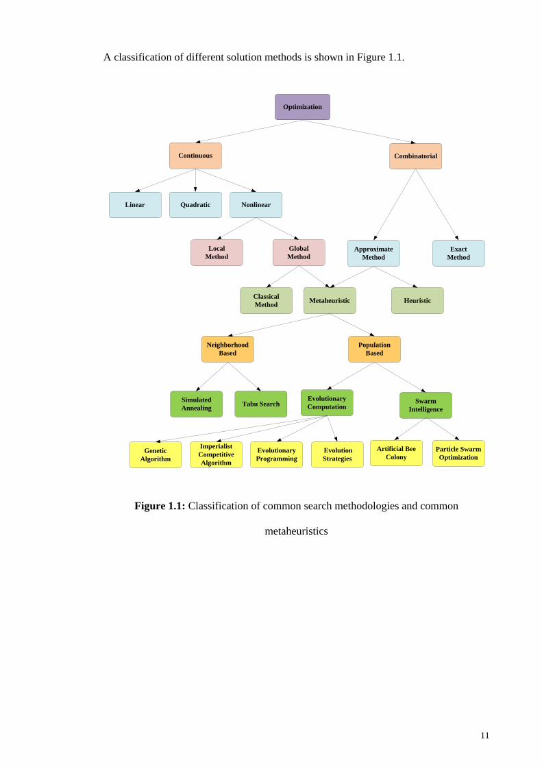
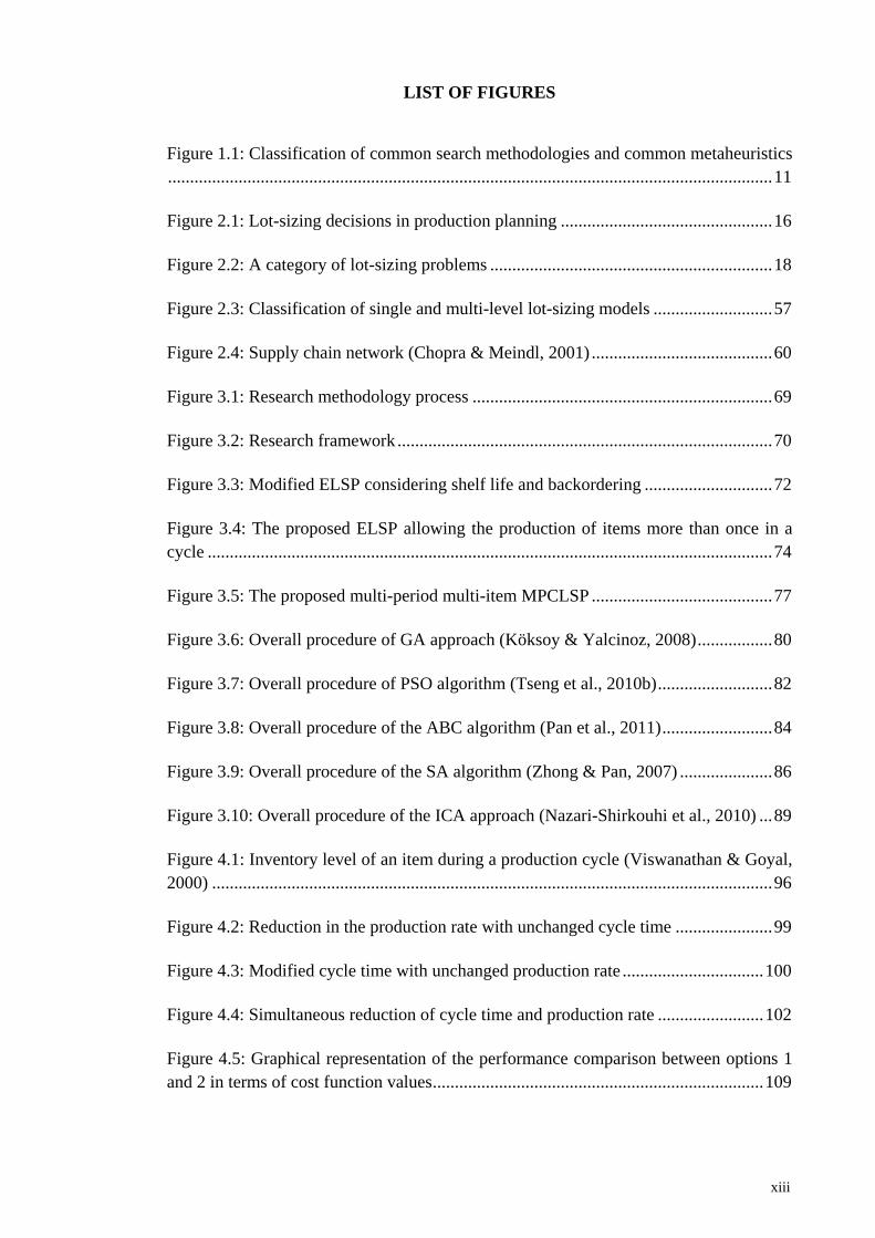
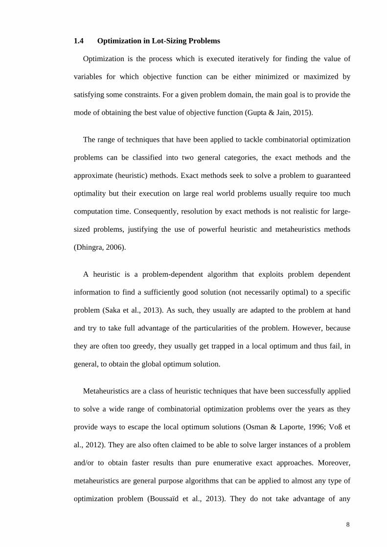
A classification of different solution methods is shown in Figure 1.1.
Optimization
Continuous Combinatorial
Linear Quadratic Nonlinear
Approximate Method
ExactMethod
Local Method
Global Method
Classical Method Metaheuristic Heuristic
Population Based
Neighborhood Based
Tabu SearchSimulated Annealing
Swarm Intelligence
Evolutionary Computation
Particle SwarmOptimization
Artificial Bee Colony
Imperialist Competitive Algorithm
EvolutionaryProgramming
Evolution Strategies
GeneticAlgorithm
Figure 1.1: Classification of common search methodologies and common
metaheuristics
11
1.5 Research Objectives
The objectives of this research are as follow:
i. To formulate and develop mathematical models for a combination of economic
lot scheduling problem, backordering and shelf life by applying three options of
“production rate reduction”, “cycle time reduction”, and “simultaneous
production rate and cycle time reduction”.
ii. To formulate and develop a mathematical model for a multi-product economic
lot scheduling problem with shelf life restrictions, backordering, and multiple
setups in a production cycle.
iii. To formulate and develop a mathematical model for a multi-period multi-
product multi-plant capacitated lot-sizing problem with inter-plant transfers in
an integrated supply chain network.
iv. To carry out optimization procedures in order to obtain the optimum or near-
optimum solutions for the proposed models by employing well-known
metaheuristic algorithms.
v. To compare the performances of the applied metaheuristic algorithms.
1.6 Scope of the Research
This work mainly expands in two directions. The first part of research focuses on the
modeling of the multi-item lot-sizing and scheduling problem in a single stage single
facility system with a continuous time scale, deterministic static demand and infinite
time horizon which is known as the ELSP with integration of multiple setups,
backordering, and shelf life. The aim is to determine the optimal lot size, production
rate, production frequency, cycle time, as well as a feasible manufacturing schedule for
the family of items, and to minimize the total pertinent cost.
12
The second part is concerned with the multi-item lot-sizing problem in a multi-stage
multi-facility system having a discrete time scale, deterministic dynamic demand and
finite time horizon. The aim is to find order, production, and shipment quantities in an
integrated production-distribution network that are optimal from a system’s perspective,
in addition to minimizing the cost of the whole supply chain.
Numerical examples are used to illustrate the features and validities of the proposed
mathematical models. To solve the models, metaheuristic algorithms namely GA, PSO,
SA, ABC, and ICA are utilized. This research aims at comparing the performance of
these metaheuristics when applied to the ELSP and MPCLSP. Applied optimizers were
written and coded in MATLAB software version R2012a (7.14.0.739) and were run on
a laptop with 2.5-GHz AMD and 4GB RAM.
1.7 Organization of the Thesis
Chapter 1 explains the background of the study, problem definition, objectives and
scope of the research.
Chapter 2 presents a critical review of available literature on single and multi-level
lot-sizing problems in single and multi-facility systems.
Chapter 3 explains the methodology of the research and research frameworks. This
chapter also provides a brief explanation of various optimization algorithms used in this
study.
Chapter 4 indicates examining and comparing three options namely “production rate
reduction”, “cycle time reduction”, and “simultaneous production rate and cycle time
reduction” in the ELSP considering shelf life and backordering.
13
Chapter 5 encompasses the proposed model formulation and development for
optimization of the ELSP with multiple setups, shelf life, and backordering using
calibrated metaheuristic algorithms. The computational results and comparisons of the
applied algorithms are also presented.
Chapter 6 describes the proposed model formulation for optimization of the
MPCLSP in an integrated supply chain network composed of multiple supplier, plants,
and distribution centers employing calibrated metaheuristic algorithms. Computational
experiments are also presented to compare the performance of the applied
metaheuristics and obtained solutions.
Chapter 7 provides the final conclusions and gives a brief summary of the study and
recommendations for future research.
14
CHAPTER 2: LITERATURE REVIEW
2.1 Introduction
In this chapter, the literature related to lot-sizing problems is reviewed. This chapter
also provides discussions on five areas related to this project: (1) Single facility lot-
sizing problems; (2) Single level lot-sizing problems; (3) Economic lot scheduling
problems; (4) Multi-level lot-sizing problems; and (5) Multi-facility lot-sizing
problems.
2.2 Lot-Sizing
There are several hierarchical levels of decisions which should be made by a
manufacturing company with its production-related activities. Strategic decisions have a
long-term scope and address questions such as what to offer on the market (product
mix), where to build plants and warehouses (location), or whether to acquire new
equipment (investment). Tactical decisions cover problems with a medium-range
impact, such as the design of facilities (layout), contracts with suppliers, and adequate
workforce levels. As for strategic choices, tactical decisions rely on aggregate data
which are demand for product families rather than single products and capacities of
entire production lines rather than particular machines (Lang, 2010).
A planning horizon of several years for strategic choices and of several months to
one year for tactical considerations makes it impossible to use detailed information.
Inputs for such decisions are therefore based on aggregated forecasts with a smaller
margin of error. As a third level, operational production planning is concerned with the
short-term implementation and execution of plans to reach the goals previously settled
on at higher levels. Establishing sequences of operations for each machine and
determining exact start and end times of operations are carried out at this level.
Operational decisions use detailed information and a finite time grid.
15
Lot-sizing problems can arise at several points in medium to short-term production
planning. Determining the production quantities for end products in the course of master
production scheduling usually covers a time span of several weeks and is based on
forecasted demand. The lot sizes of end products directly affect the demand for the
components from which they are assembled. In the course of the subsequent material
requirements planning, lots for subassemblies and parts, as well as orders for raw
materials, can be coupled, which thus gives rise to lot-sizing problems farther down the
product structure. Lot-sizing decisions can also be integrated with sequencing and
scheduling decisions. The time span considered in such a case is very short, and the
resulting production plan usually covers about a week period. Figure 2.1 (based on Bahl
et al., 1987; Tempelmeier, 1997; Lang, 2010) provides a quick overview of production
planning decisions with an emphasis on lot-sizing.
Long-term decisions
Medium-term decisions
Short-term decisions
Master Production Schedule
Material Requirements Planning
Capacity Requirements Planning
Lot sizing for end products
Integrated lot sizing and scheduling
Aggregation Scope
None
High
Days
Weeks
Month
Years
Lot sizing for components
Machine scheduling
Figure 2.1: Lot-sizing decisions in production planning
16
Bahl et al. (1987) classified lot-sizing problems into four categories:
i. Single level unconstrained resources
ii. Single level constrained resources
iii. Multi-level unconstrained resources
iv. Multi-level constrained resources
Levels denote the different stages in a bill of material structure where there are
dependencies of requirements, and constrained resources stand for production capacity
restrictions (Woarawichai et al., 2010).
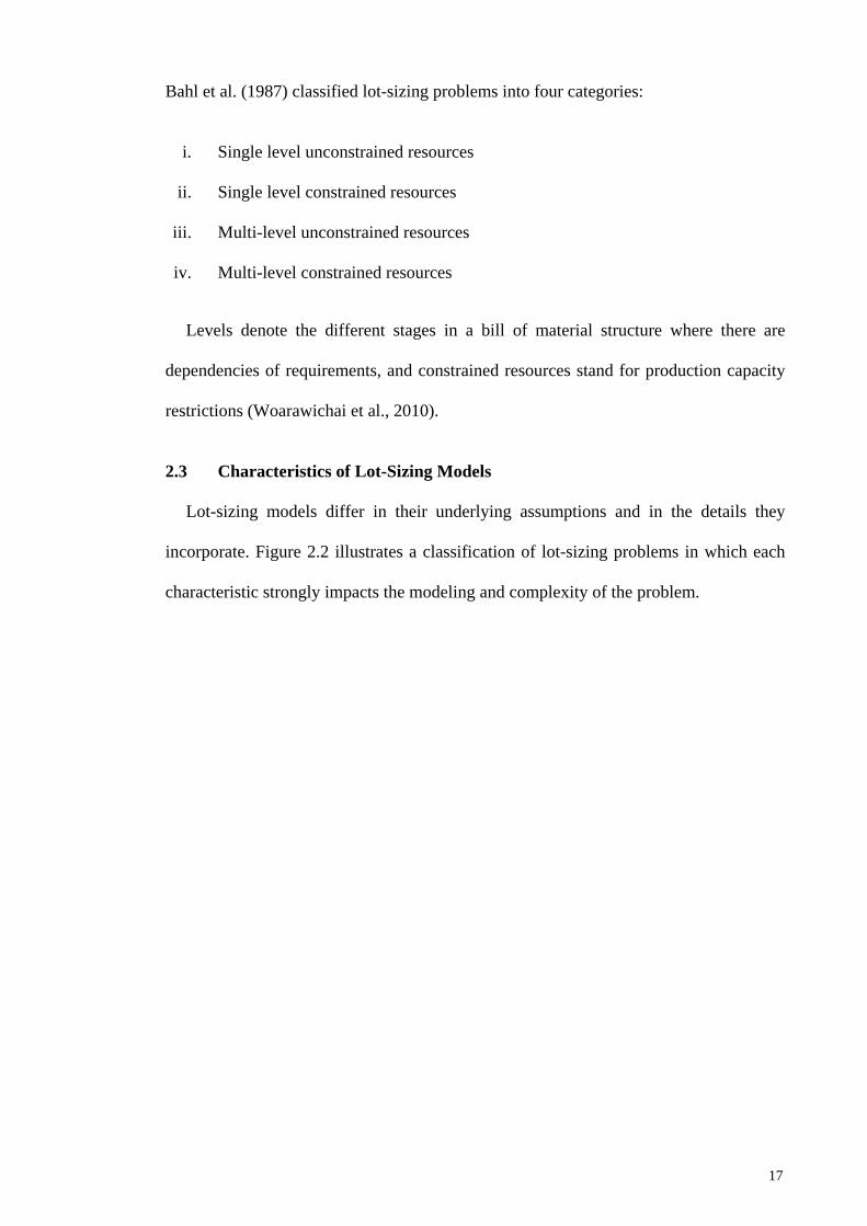
2.3 Characteristics of Lot-Sizing Models
Lot-sizing models differ in their underlying assumptions and in the details they
incorporate. Figure 2.2 illustrates a classification of lot-sizing problems in which each
characteristic strongly impacts the modeling and complexity of the problem.
17
Lot-sizing problems
Multi-facilitySingle facility
Single level Multi-level Multi-level
Single item Multi-item
Uncapacitated Capacitated
Deterministic demand
Stochastic demand
Static demand
Dynamic demand
Figure 2.2: A category of lot-sizing problems
Lot-sizing problems can be characterized by a variety of aspects and classification
criteria, which are explained in the following subsections.
2.3.1 Planning Horizon
A planning horizon is the length of time into the future for which plans are made.
The length of the horizon can be finite or infinite. A finite planning horizon is typically
accompanied by a time-varying demand and an infinite planning horizon by a constant
demand rate. Furthermore, the time horizon can be divided into discrete or continuous
time periods.
As defined by Belvaux and Wolsey (2000), lot-sizing problems can be either small
bucket or big bucket. Big bucket problems allow for the production of many items at the
same time period without taking into account sequencing issues. Small bucket models
18
considers short time periods in order to be able to model start-ups, switch-offs and/or
changeovers. The small bucket models are then split further into those in which only
one item can be setup per period, and those with possibly two setups per period.
2.3.2 Number of Products
Single item models consider one type of product at a time. Multi-item models
consider a number of products simultaneously. These products must have at least one
interrelating or binding factor such as budget, capacity constraint, or a common setup.
2.3.3 Number of Levels
If multiple items are considered, they can either be from a single level of the product
structure, i.e. multiple independent final products are considered, or they can be on
different levels, i.e. parent-component relationships between the items are present. In
such multi-level production systems, end products are assembled from intermediate
products (sub-assemblies), which might in turn require raw materials or parts for
production. The output of one stage is thus the input for the next stage.
2.3.4 Capacity Constraints
Resources in a manufacturing system contain manpower, equipment, machines,
budget, and so forth. If the models assume unlimited capacities of resources, they are
considered as uncapacitated problem. Capacitated models recognize that some resources
are given in a limited number or amount so that planning and scheduling systems need
to avoid over utilizing these resources.
In some cases, it is essential to consider capacity utilization more accurately in order
to achieve a feasible production plan. For instance, the capacity utilized when a machine
begins or finishes a production batch, or when a machine shifts from one product to
19
another, may need to be considered. In such cases, models deal with setup times,
changeover times, or sequencing restrictions.
2.3.5 Setup Structure
A particular setup is often necessary to prepare a machine for the production of a
specific product if this machine produces different types of products. Whenever this
changeover causes setup times and/or cost, a lot-sizing problem arises.
Setup times implies the capacity consumed because of cleaning, warming, machine
adjustments, calibration, inspection, test runs, tool changes, and so forth, when the
production for a new product begins. Setup times can be included explicitly in a model.
However, due to the complexity in such a case, they are often incorporated indirectly
via the setup costs (Jans & Degraeve, 2008). Setup costs and setup times, are generally
modeled by considering zero-one variables in the mathematical models and make the
problem solving harder.
2.3.6 Demand
Another important characteristic of lot-sizing problem is the nature of demand. Static
demand models assume that parameter’s value does not vary over the planning horizon,
while dynamic demand models allow for variation over time. If the demand value is
known in advance, the demand stream is considered as deterministic. If the demand is
based on distribution or a measure of uncertainty, it is considered as stochastic.
Independent demand refers to the demand for a product which is independent of
demand for other items. Independent demand for end products is triggered by the
market. Dependent demand for components is triggered by scheduled production on
superior levels.
20
2.3.7 Inventory Shortage
Shortage occurs when demand exceeds the available inventory for an item, and can
be divided into two categories, namely backordering and lost sale. Backordering occurs
when it is probable to fulfill demand of the current period in the next time period. If
demand cannot be satisfied at all, lost sale can happen. The combination of
backordering and lost sale is also plausible. However, both cases incur penalty cost as
they have a negative impact on customer satisfaction.
2.3.8 Deterioration
Another aspect that affects the problem complexity is deterioration or shelf life
constraint where items can be held only for a limited lifetime. Deterioration refers to a
process in which inventories undergo a change in storage over time, such that they
become partially or completely unsuited for consumption and therefore, may impose
additional costs for inventory storage. Ignoring deterioration of the items may bring
about misleading replenishment policies and shortage in demand which in turn incurs
additional shortage cost.
2.4 Single Facility Problems
The classical concept of a single facility can be considered as a single machine or
may be defined as a complete assembly line that would in essence form the whole
physical plant (Aras & Swanson, 1982). According to Kreipl and Pinedo (2004), a
short-term detailed scheduling model is generally only concerned with a single facility,
or, at most, with a single stage. Such a model usually takes more detailed information
into account than a planning model.
Based on Bruggeman et al. (1982) and Glock et al. (2014), when there is only a
single facility or production line, only one product can be in production at a time. For a
multi-item environment, production needs to be scheduled in such a way that the
21
machine is never required to produce more than a single product at a time. Therefore, to
generate a feasible manufacturing schedule, the production cycle of the items requires to
be modified in order to prevent overlaps in the schedule.
Single facility problems have been reviewed broadly in both single and multi-level
systems, which are explained as follow.
2.4.1 Single Level Lot-Sizing Problems
In single level structures (also known as single stage), demand for an item is obtained
directly from customer orders and/or market forecasts. Single stage lot-sizing problems
in procurement/distribution environments typically concern only purchasing and
holding costs and avoid transportation cost. Anderson et al. (1997) defined single stage
production systems as those which require one operation for each job involving either a
single machine, or more than one machine operating in parallel. Nevertheless, each of
the parallel machines has exactly the same function.
In the following subsections, the literature related to uncapacitated and capacitated
single level lot-sizing problems is reviewed.
2.4.1.1 Uncapacitated Single Item Problem
The single level single item problems with no capacity constraint were at the advent
of developments in the lot-sizing and scheduling arena. The EOQ model was introduced
by Harris (1913), which assumes a constant demand rate for a single item, infinite
planning horizon, and continuous time scale with the aim of minimizing the sum of
ordering and inventory holding costs. Wagner and Whitin (WW) (1958) investigated the
lot-sizing problem for a single item with unlimited capacities over a finite planning
horizon divided into discrete periods. Demand and costs were accordingly time-varying.
22
Numerous model formulations and solution procedures have been proposed for the
uncapacitated single item lot-sizing problems.
Zangwill (1969) improved the WW basic model to include backlogging of demand.
Approximate solutions to the single item, single stage uncapacitated lot-sizing problem
were suggested by DeMatteis (1968) and Silver and Meal (1973). The major advantage
of these approaches is that they are computationally much more efficient than the exact
solutions. Hax and Candea (1984) extended the EOQ model by allowing backlogging,
lost sales, and quantity discounts. Fordyce and Webster (1985) modified the WW
algorithm for situations in which unit cost price is not constant over the planning
horizon, and included quantity discounts. Lev and Weiss (1990) and Gascon (1995)
presented solutions for the finite horizon EOQ model where costs are time-dependent.
Discounts are a primary marketing mechanism for inducing customers to increase the
size of their purchases. Quantity discounts from suppliers and freight discounts from
shippers are commonly encountered by organizations. Tersine and Barman (1991)
structured quantity and freight discounts into the order size decision in a deterministic
EOQ system. Optimum lot-sizing algorithms were derived for the dual discount
situations of all-units or incremental quantity discounts and all-weight or incremental
freight discounts.
Gupta and Brennan (1992) introduced an easy alternative to the WW backorder
algorithm. The performance of the model was compared with several of the traditional
lot-sizing rules (lot for lot, EOQ, period order quantity, least unit cost, least total cost,
part period algorithm, Silver-Meal algorithm, and WW algorithm) as well as the
backorder versions of WW and EOQ. It was concluded that the proposed algorithm is
sufficiently robust and relatively easy to apply. Most of the dynamic lot-sizing models
assume that production is performed on reliable machines. Kuhn (1997) analyzed the
23
effects of setup recovery with machine breakdowns and corrective maintenance for the
single item uncapacitated lot-sizing problem. In a first case, the assumption was made
that the setup is totally lost after a breakdown. In a second case, the costs of resuming
production of the same item after a breakdown was lower compared to the original setup
cost.
Agra and Constantino (1999) examined the single item uncapacitated lot-sizing
problem with backlogging and start-up costs where WW costs were assumed.
Hernandez and Suer (1999) presented a GA approach to obtain the order quantities for a
single item, single level uncapacitated lot-sizing problem. In the experimentation,
different strategies were presented to evaluate the behavior of the GA under different
parameters sets. The results showed that the proposed procedure generated satisfactory
solutions to the considered problem. Richter and Sombrutzki (2000) studied the reverse
WW dynamic production planning and inventory control model. In such reverse
(product recovery) models, used products arrive to be stored and to be remanufactured
at minimum cost. It was assumed that the demand can be met either from newly
manufactured products or from return products which have been remanufactured.
Lee et al. (2001) discussed the single item, uncapacitated dynamic lot-sizing problem
with a demand time window, where for each demand an earliest and latest delivery date
is specified and the demand can be satisfied in the defined period without penalty. It
was shown that there exists an optimal solution in which demand is not split, where the
complete demand for a specific order can be covered by production from the same
period. Loparic et al. (2001) proposed valid inequalities for solving a variant of the
single item uncapacitated lot-sizing model of the WW problem involving sales instead
of fixed demands and lower bounds on the stock variables. Aksen et al. (2003)
introduced a profit maximization version of the WW model for the deterministic single
24
item uncapacitated lot-sizing problem with lost sales. It was assumed that demand
cannot be backlogged, and costs and selling prices are time-variant. A forward recursive
dynamic programming (DP) algorithm was developed to solve the problem optimally.
Teunter and Flapper (2003) examined a single stage single product production
system, where produced units can be non-defective, reworkable defective, or non-
reworkable defective. De Toledo and Shiguemoto (2005) proposed an efficient
implementation of a forward DP algorithm for solving the lot-sizing problems in a
single production center. Brahimi et al. (2006) reviewed various solution methods for
solving the single item uncapacitated lot-sizing problem. Chiu (2008) presented a
simple algebraic method to replace the use of calculus for determining the optimal lot
size. Gutiérrez et al. (2008) addressed the dynamic lot-sizing problem with time-varying
storage capacities with the aim of minimizing the total cost including setup, holding,
and production/ordering costs.
Gaafar et al. (2009) applied the SA algorithm to find the solution of the deterministic
dynamic lot-sizing problem with batch ordering and backorders, and compared the
performance of the proposed SA with GA and modified Silver-Meal heuristic. Results
indicated that SA algorithm had the best performance, followed by the GA, in terms of
the frequency of obtaining the optimum solution and the average deviation from the
optimum solution. It was also shown that SA was the most robust of the investigated
heuristics as its performance was only affected by the length of the planning horizon.
Hwang and van den Heuvel (2009) proposed a DP algorithm to optimally solve the
classical uncapacitated single item lot-sizing problem with lost sales, upper bounds on
stocks and concave costs. Vargas (2009) presented an algorithm for determining the
optimal solution for the stochastic version of the WW dynamic lot-sizing problem.
25
Sana (2010) investigated an economic production lot size model in an imperfect
production system in which the production facility may shift from an “in-control state”
to an “out-of-control” state at any random time. In long-run process, the process shifts
from the in-control state to the out-of-control state after certain time due to higher
production rate and production run time. The proposed model was formulated assuming
that a certain percent of total product is defective (imperfect), in out-of-control state,
which varies with production rate and production-run time. The objective was to
minimize the total cost including manufacturing cost, setup cost, holding cost, and
reworking cost of imperfect quality products.
Senyiğit (2010) proposed a heuristic approach to solve the dynamic lot-sizing
problem with demand and purchasing price uncertainties. Well-known least unit cost
and Silver-Meal algorithms were also modified for both time-varying purchasing price
and rolling horizon. The proposed heuristic was basically based on a cost-benefit
evaluation at decision points. Absi et al. (2011) considered the single item uncapacitated
lot-sizing problem with production time windows, lost sales, early productions, and
backlogs. Several properties of the optimal solution for different variants of the problem
when production time windows are non-customer specific were presented. The DP
algorithm was used to solve the proposed problem.
2.4.1.2 Uncapacitated Multi-Item Problem
The principal concern of this category is to obtain production or order quantity for
multiple products so as to minimize the long run average cost for the family of items
and meet demand over the defined horizon. The total cost typically involves
setup/ordering, inventory, and production/purchasing costs. Based on the absence of
capacity constraints and parent-component relationships between products, decisions
can be made for each item independently.
26
However, the existence of joint setup/ordering costs causes the interdependency
between products which is known as the economic order quantity with joint
replenishment problem. In a multi-item environment with a joint setup cost structure
considerable savings may be realized by coordinating the replenishments (Aksoy &
Erenguc, 1988). In the joint replenishment problem (JRP), major setup occurs if
production is started, and minor setups are required if the processor switches from one
item to the next (Graves, 1981). The aim of the model is to find the joint frequency of
production/order cycles and the frequency of producing/purchasing each product in
addition to minimizing the total cost. An overview of the JRP and solution methods can
be found in Goyal and Deshmukh (1992). Later, Goyal and Deshmukh (1993) proposed
heuristic procedures for solving the JRP.
Aksoy and Erenguc (1988) differentiated between the deterministic and stochastic
and between the static and dynamic JRP. They developed a DP approach for small size
static-dynamic JRP and a heuristic method for large family sizes. Van Eijs et al. (1992)
distinguished between two different types of strategies, namely direct grouping
strategies and indirect grouping strategies, for the multi-item inventory systems having
constant deterministic demand and joint replenishment costs. The performances of the
strategies were measured as the percentage cost savings of a joint replenishment
strategy relative to an independent strategy, and were quantified through simulation.
Federgruen and Tzur (1994) addressed the JRP, where in the presence of joint setup
costs, dynamic lot-sizing schedules need to be determined for multiple items over a
finite planning horizon with general time-varying cost and demand. They developed a
partitioning heuristic for the proposed problem, which partitions the complete horizon
of periods into several relatively small intervals, and solved the problem via an efficient
branch and bound method.
27
Hariga (1994) studied the effects of inflation and time value of money on the
replenishment policies of items with time continuous non-stationary demand over a
finite planning horizon. He developed the DP models for the commonly used
replenishment policies in the inventory lot-sizing literature with time-varying demand
and shortages. The results showed that the initial cycle length is virtually insensitive to
the type of replenishment policy. They also extended the developed models to more
practical inventory situations with exponentially deteriorating items and perishable
products having fixed life time.
Kirca (1995) considered the multi-item dynamic lot-sizing problem with joint set-up
costs. A tight formulation of the problem and the dual of the linear relaxation of this
formulation were presented. A procedure to solve the dual problem was developed,
where the solution provided a strong lower bound for the proposed problem. The
computational experiments revealed that the proposed approach outperforms the branch
and bound algorithm.
2.4.1.3 Capacitated Single Item Problem
Capacitated restrictions enhance the complexity of lot-sizing problems. The objective
of this group of lot-sizing problem is to obtain the optimal production quantity or order
size for a single product that minimizes the total cost including setup/ordering,
inventory, and production/purchasing costs, while meeting the known demands and
satisfying capacity constraints over the planning horizon.
Lambrecht and Vanderveken (1979) developed a computationally efficient algorithm
for solving a single item dynamic lot-sizing problem with capacity constraints in order
to obtain an optimum production schedule that minimizes the total production and
inventory costs. Reviews of the literature for this class of problem can be found in Drexl
28
and Kimms (1997) and Karimi et al. (2003), who offered overviews of optimal and
heuristic solution procedures.
Examples of problems and related modeling approaches for dynamic capacitated lot-
sizing in a single level system with discrete time representation are the ELSP (Rogers,
1958), continuous setup and lot-sizing problem (CSLP) (Karmarkar & Schrage, 1985),
capacitated lot-sizing problem (CLSP) (Günther, 1987), discrete lot-sizing and
scheduling problem (DLSP) (Fleischmann, 1990; Salomon et al., 1991), proportional
lot-sizing and scheduling problem (PLSP) (Haase, 1994; Drexl & Haase, 1995), and
capacitated lot-sizing problem with sequence-dependent setups (CLSD) (Haase, 1996).
The DLSP allows for the production of only one item in each period. The production
is further assumed to be “all or nothing”, and the total capacity available per period is
used for the production of the scheduled item. The CSLP is equivalent to the DLSP
without the “all or nothing” requirement, which can lead to periods with some slack
capacity. The PLSP goes one step further and allows for the production of a second item
to avoid excessive idle time on the resource. The CLSD assumes a fixed lead time offset
of one (macro) period in order to secure a feasible material flow between production
stages while small bucket models usually only require a micro period as a fixed lead
time offset.
Fleischmann and Meyr (1997) integrated all mentioned models (ELSP, CSLP, CLSP,
DLSP, PLSP, and CLSD) within the general lot-sizing and scheduling problem (GLSP).
They used a two-fold time structure, where each macro-period is divided into several
micro-periods of variable length. A complete sequence of items was established. All
mentioned models commonly consider that setup times can only be considered if they
do not exceed the length of a period. However, Koçlar and Süral (2005), through a
simple modification of the GLSP, showed that setup times exceeding the length of a
29
period can also be incorporated. The capacitated lot-sizing problem with linked lot sizes
(CLSPL) (Suerie & Stadtler, 2003), extends the CLSP with the possibility of setup
carryover. The CLSPL belongs to the class of large bucket problems, which allow many
setup operations within a single period.
Florian et al. (1980) and Chen and Thizy (1990) proved that the single item CLSP is
NP-hard. To deal with the intricacy of the problem and find the optimal solution in
reasonable amount of time, numerous studies have applied heuristic and metaheuristic
algorithms. Gavish and Johnson (1990) proposed a fully polynomial approximation
scheme for solving the single item CLSP. However, their approach is more suitable for
continuous models. Sandbothe and Thompson (1990) included backordering into the
single item CLSP, and presented a polynomial algorithm for solving the case of
constant capacities and a heuristic algorithm for solving the variable production
capacity.
Kirca (1990) developed a DP-based algorithm for the single item lot-sizing problem
with concave costs and arbitrary capacities. The performance of the algorithm was
compared with the performance of the existing procedures in the literature for the
general, the constant capacity, and the constant unit cost problems. The computational
results demonstrated that proposed algorithm is at least three times faster than the other
procedures for all problem types considered. Chen et al. (1994) developed a DP method
for the single item capacitated dynamic lot size model with non-negative demands and
no backlogging. The proposed approach produced the optimal value function in
piecewise linear segments.
Chung (1994) studied a deterministic single product capacitated dynamic lot size
model with linear production and holding costs where the setup costs, unit production
costs, and capacities are arbitrary functions of the period, and the unit production costs
30
satisfy the constraint. To solve the problem, the DP algorithm was combined with
branch and bound approach. Lotfi and Yoon (1994) considered a multi-period single
item production scheduling problem with a deterministic time-varying demand pattern
and concave cost functions. Optimal production lot sizes were determined subject to
dynamic production capacity and no backlogs in addition to minimizing the total costs
of production, setup, and inventory. The proposed algorithm was tested extensively by
solving several randomly generated problems with varying degrees of complexity, and
showed quite good performance for practical applications.
Hindi (1995a) considered a capacitated single item lot-sizing model where a startup
cost is incurred for switching the production facility on, and a separate reservation cost
is incurred for keeping the facility on whether it is used for production or not. A tabu
search (TS) scheme was developed for solving the problem which was capable of
reaching the optimal solution for a large number of varied problem instances. Hardin et
al. (2007) analyzed the quality of lower and upper bounds provided by a range of fast
algorithms for single item CLSP with time-varying demands.
Akbalik and Pochet (2009) provided valid inequalities for the single item CLSP with
step-wise production costs. Constant-sized batch production was carried out with a
limited production capacity in order to satisfy the customer demand over a finite
horizon. They suggested a cutting plane algorithm for different classes of the proposed
valid inequalities. Computational results showed the efficiency of the proposed
algorithm compared to the existing methods. Hellion et al. (2012) examined the single
item CLSP with concave production and storage costs, and minimum order quantity.
They proposed a polynomial time algorithm to solve the problem optimally, and
computationally tested the algorithm on various instances.
31
2.4.1.4 Capacitated Multi-Item Problem
The multi-item CLSP is the extension of the WW problem to multiple items and
consequently limited capacities in each period. The CLSP is referred to as a big bucket
problem since several items may be produced per period. The aim of the classical single
level CLSP is to determine the quantities and timing of production batches in order to
satisfy external requirements while incurring minimum costs. No backlogging is
allowed and sequencing decisions are not included into this problem. The overall model
of this category of lot-sizing problem is presented below (Based on Drexl & Kimms,
1997; Pochet, 2001; Karimi et al., 2003).
(a) Assumptions of the CLSP
i. The planning horizon is finite and divided into big time buckets.
ii. The lots are determined for multiple items without any interrelationships. The
model thus considers a single production level.
iii. The external demand for the items is dynamic and deterministic, and has to be
satisfied immediately and completely.
iv. The standard model allows no backordering (delaying fulfillment) or lost sales
(no fulfillment).
v. There is a single resource with limited capacity that is shared by all items.
vi. Overtime decisions are not considered in the standard version.
vii. For every item produced in a given period, one setup takes place. The current
setup state of the resource has no influence on setting it up for the next item. The
setups are sequence-independent, postponing the scheduling decision.
viii. The setup state of the resource at the end of a period does not extend to the
beginning of the subsequent period. This means that there is no possibility of a
setup carryover, and not even a partial sequence is established.
32
ix. Setup times are not included as such. Instead of modeling them explicitly, they
are hidden in the setup costs, represented as opportunity costs accounting for the
time lost to actual production.
x. Variable production costs, holding costs and setup costs can either be modeled
to vary with time, or they can be modeled static throughout the planning
horizon. The time-invariant production costs and the respective term in the
objective function can be omitted from the model as the total amount of
production for each item is predetermined by the sum of its external demand.
The objective of the CLSP is to minimize all costs incurred throughout the
planning horizon.
(b) Indices
i index for item (i = 1, … , N)
t index for period (t = 1, … , T)
(c) Parameters
dit External demand for item i in period t
Ct Available capacity in time units in period t
Ri Capacity in time units needed to produce one unit of item i
Oit Variable production cost for one unit of item i in period t
Sit Setup cost for item i in period t
Hit Holding cost for one unit of item i in period t
Mit Upper bound on the production quantity of item i in period t
(d) Decision Variables
Qit Production quantity (lot size) of item i in period t
Iit Inventory level of item i at the end of period t
33
if item is produced in per1 i.e. >0)0 oth
iod (erwise
itit
Qi tY
=
(e) Mathematical Formulation
Using the above notations, the mathematical model for the CLSP is presented below.
1 1Minimize
N T
it it it it it iti t
S Y O Q H I= =
+ +∑∑ (2.1)
Subject to:
1
N
i it ti
R Q C=
≤∑ (2.2)
( 1)it i t it itI I Q d−= + −
(2.3)
it it itQ M Y≤
(2.4)
min ,T
it t i itt t
M C R d ′′=
=
∑ (2.5)
1 0iI =
(2.6)
, 0it itX I ≥
(2.7)
= 0,1itY
(2.8)
The objective function in Eq. (2.1) minimizes the total cost that includes setup,
production, and inventory costs. Equation (2.2) represents the capacity constraint. The
overall consumption for production must be lower than or equal to the available
capacity. Equation (2.3) concerns the inventory balance equation. Equation (2.4) relates
the binary setup variable Yit to the production variable Qit. It means that when there is
production in period t, Yit must be equal to 1. In other words, production of an item is
only possible if the resource has been setup for that item. If no setup takes place (Yit =
0), no production can take place (i.e. Qit = 0). The upper bound on the production, Mit,
is either given by the remaining unfulfilled demand or by the available capacity as
34
shown in Eq. (2.5). Equation (2.6) shows that the inventory of item i for period 1 is
zero. Equation (2.7) indicates that all decision variables are non-negative. Equation
(2.8) shows Yit is defined as the binary variable.
Many heuristic techniques have been developed for solving the variations of single
level CLSP. Dixon and Silver (1981) developed a heuristic for solving the multi-item
single level lot-sizing problem with limited capacity in a single facility production
system, where the time required to setup the facility was avoided. The objective was to
determine lot sizes so that costs are minimized, no backlogging occurs, and capacity is
not exceeded. The results indicated that the proposed heuristic will usually generate a
very good solution with a relatively small amount of computational effort.
Thizy and van Wassenhove (1985) designed a Lagrangian relaxation (LR) approach,
in which capacity constraints are relaxed, in an attempt to decompose the problem into
some uncapacitated single item lot-sizing sub-problems, solvable by the WW algorithm.
The proposed method incorporated a primal partitioning scheme with a network flow
sub-problem to obtain good feasible solutions.
A review of the CLSP can be found in Maes and van Wassenhove (1988), which was
focused on heuristic solution procedures compared in extensive numerical studies. The
authors classified the existing approaches into single resource and mathematical
programming-based heuristics. De Souza and Armentano (1994) presented a multi-item
CLSP with setup times for production of items, which was constrained by a limited
regular time and a limited overtime as well as a limitation on production level of any
item in a given period. The proposed problem was tackled by a cross decomposition
based algorithm, which can provide optimal or near optimal solutions if computation
time is restricted.
35
Millar and Yang (1994) developed both the LR and Lagrangian decomposition
approaches to solve the single level CLSP with backordering. Computational analysis
showed that both algorithms are quite effective, particularly when item setup and unit
backorder costs are high. Hindi (1995b) addressed the problem of multi-item dynamic
lot-sizing in the presence of a single capacitated resource. A model based on variable
redefinition was developed leading to a solution strategy based on a branch and bound
search with sharp low bounds. The resulting solution scheme was very efficient in terms
of computation time. The standard CLSP was tackled by Hindi (1996), who combined
the TS algorithm on the setup pattern for solving a reformulation of the problem as an
uncapacitated transshipment problem.
Özdamar and Bozyel (2000) extended the CLSP to include overtime decisions and
capacity consuming setups with the objective of minimizing inventory holding and
overtime costs. Heuristic approaches such as hierarchical production planning approach,
a GA approach based on the transportation-like formulation of the single item
production planning model with dynamic demand, and a SA algorithm based on shifting
family lot sizes among consecutive periods were developed to deal with the proposed
problem. Computational results demonstrated that the SA approach produced high
quality schedules and was computationally more efficient.
Özdamar et al. (2002) integrated the GA with TS and SA algorithms (GATA) to
solve the CLSP with overtime and setup times. It was assumed that setups do not incur
costs other than lost production capacity and therefore, setups contribute to total costs
implicitly via overtime costs whenever capacity bottlenecks occur. The proposed GATA
integrated the powerful characteristics of all three search algorithms, and the results
demonstrated that GATA outperformed other heuristics reported in Özdamar and
Bozyel (2000). Xie and Dong (2002) proposed a GA for solving the CLSP by designing
36
a domain-specific encoding scheme for the lot sizes and by providing a heuristic
shifting procedure as the decoding schedule. They designed the presentation technique
that encoded only the binary variables for the setup patterns, but derives other decision
variables by making use of the problem-specific knowledge.
Hindi et al. (2003) examined the multi-item single level CLSP with setup times. A
lower bound on the value of the objective function was calculated by the LR approach
with sub-gradient optimization. During the process, attempts were made to obtain
feasible solutions through a smoothing heuristic, followed by a local search with a
variable neighborhood search (VNS). Solutions found were further optimized by
solving a capacitated transshipment problem.
Liu et al. (2004) studied single item inventory capacitated lot size model with lost
sales. Gupta and Magnusson (2005) examined the capacitated lot-sizing and scheduling
problem with sequence-dependent setup costs and non-zero setup times, with the
additional feature that setups may be carried over from one period to the next, and that
setups are preserved over idle periods. They developed a heuristic for solving large
problem instances, and coupled with a procedure for obtaining a lower bound on the
optimal solution. It was shown that the heuristic is more effective when there are many
more products than there are planning periods.
Song and Chan (2005) investigated a single item lot-sizing problem with
backlogging on a single machine at a finite production rate. The objective was to
minimize the total cost of setup, stockholding and backlogging to satisfy a sequence of
discrete demands. Both varying demands over a finite planning horizon and fixed
demands at regular intervals over an infinite planning horizon were considered. A DP
algorithm was proposed for the computation of an optimal production schedule for the
varying demands case and a simpler one for the fixed demands case.
37
Jodlbauer (2006) developed a non-time discrete approach for an integrated planning
procedure, and applied to a multi-item capacitated production system with dynamic
demand. The objective was to minimize the total costs, which consist of holding and
setup costs for one period. The proposed approach was based on a specific property of
the setup cost function, which allows for replacement of the integer formulation for the
number of setup activities in the model.
Federgruen et al. (2007) developed a progressive interval heuristic for the multi-item
CLSP with deterministic demand, joint and item-dependent setup cost with the aim of
finding a lot-sizing strategy that satisfies the demands for all items over the entire
horizon without backlogging, and minimizing the sum of inventory-carrying costs,
fixed-order costs, and variable-order costs. Marinelli et al. (2007) proposed a solution
approach for a capacitated lot-sizing and scheduling real problem with parallel
machines and shared buffers, arising in a packaging company producing yoghurt. An
effective two-stage optimization heuristic based on the decomposition of the problem
into a lot-sizing problem and a scheduling problem was developed. The proposed
heuristic showed near-optimal solutions, all obtained in a short computation time.
Jans and Degraeve (2008) presented an overview of developments in the field of
modeling of the deterministic single level dynamic lot-sizing problems, where focus
was on the modeling of various industrial extensions rather than the solution
approaches. Quadt and Kuhn (2008) provided reviews of extensions of the basic CLSP
including parallel machines, backorders, and setup times, and illustrated model
formulations for each of the extensions. Absi and Kedad-Sidhoum (2009) addressed a
multi-item CLSP with setup times, safety stock and demand shortages. It was assumed
that demand cannot be backlogged, but can be totally or partially lost. A LR procedure
for the resource capacity constraints and a DP algorithm to solve the induced sub-
38
problems were developed. Some experimental results showed the effectiveness of the
proposed approaches.
Anily et al. (2009) examined a multi-item lot-sizing problem with joint setup costs
and constant capacities. Apart from the usual per unit production and storage costs for
each item, a setup cost was incurred for each batch of production. Computational results
were presented to test the effectiveness of using the tight linear programs in
strengthening the basic mixed integer programming formulations of the joint setup
problem both when the storage cost conditions are satisfied, and also when they are
violated.
Pan et al. (2009) addressed the capacitated dynamic lot-sizing problem arising in
closed-loop supply chain where returned products are collected from customers. It was
assumed that returned products can either be disposed or be remanufactured to be sold
as new ones again; hence the market demands can be satisfied by either newly produced
products or remanufactured ones. The proposed problem was analyzed and solved using
DP algorithms under different scenarios. It was shown that the problem with only
disposal or remanufacturing can be converted into a traditional CLSP and be solved by
a polynomial algorithm if the capacities are constant. A pseudo-polynomial algorithm
was proposed for the problem with both capacitated disposal and remanufacturing. It
was indicated that the proposed algorithms perform well when solving problems of
practical sizes.
Buschkühl et al. (2010) differentiated solution procedures for the CLSP into
mathematical programming-based approaches, Lagrangian heuristics, decomposition
and aggregation heuristics, metaheuristics, and problem specific greedy heuristics. They
have also discussed both different modeling approaches to the optimization problems
and different algorithmic solution approaches. Zhang et al. (2012) proposed a LR-based
39
solution approach to solve a mixed integer CLSP in a closed-loop supply chain
considering setup costs, product returns, and remanufacturing. Numerical experiments
using synthesized data demonstrated that proposed approach can find quality solutions
efficiently.
Ramezanian et al. (2013) presented a mathematical model for integrating lot-sizing
and scheduling problem in capacitated flow shop environments. Two mixed integer
programming-based approaches with rolling horizon framework were used to solve the
proposed model. Mehdizadeh and Fatehi Kivi (2014) proposed a new mixed integer
programming model for multi-item CLSP with setup times, safety stock and demand
shortages in closed-loop supply chains. The returned products from customers can
either be disposed or be remanufactured to be sold as new ones again. Due to the
complexity of problem, three metaheuristics algorithms namely SA, vibration damping
optimization algorithm and harmony search algorithm were used to solve the model.
The results confirmed the efficiency of the harmony search algorithm against the other
methods.
Chan et al. (2015) explored the multi-item CLSP by addressing the backlogging and
associated high penalty costs incurred. At the same time, penalty cost for exceeding the
resource capacity was also taken into account. To solve this computationally complex
problem, a less explored algorithm biased random key GA was applied. The results
showed that the proposed algorithm is an efficient tool to tackle such complex
problems.
De Reyck (2015) developed period decompositions for the CLSP with setup times.
Based on two strong reformulations of the problem, a transformed reformulation and
valid inequalities were presented that speed up column generation and the LR approach.
An efficient hybrid scheme was proposed that combines column generation and the LR
40
in a novel way. Computational experiments showed that the proposed solution method
for finding lower bounds is competitive with the available approaches in the literature.
Hajipour et al. (2015) considered a multi-item CLSP with setup times, safety stocks,
and demand shortages plus lost sales and backorder considerations for various
production methods (i.e., job shop, batch flow, and continuous flow among others).
Two novel Pareto-based multi-objective metaheuristic algorithms were proposed,
namely multi-objective vibration damping optimization and multi-objective harmony
search algorithm. The proposed algorithms were compared with two well-known
evolutionary algorithms called the non-dominated sorting the GA and multi-objective
SA to demonstrate the efficiency and effectiveness of the proposed methods.
Tempelmeier and Hilger (2015) proposed the stochastic dynamic lot-sizing problem
with multiple items and limited capacity under two types of fill rate constraints. They
proposed linear programming (LP) models, where the non-linear functions of the
expected backorders and the expected inventory on hand were approximated by
piecewise linear functions. The models were solved with a variant of the fix-and-
optimize heuristic.
2.4.2 Economic Lot Scheduling Problem
The ELSP is concerned with scheduling the production of multiple items in a single
facility on a periodical basis with the restriction that one item is produced at a time. The
objective of the ELSP is to determine the lot size and the schedule of production of each
product so as to minimize the long run average costs incurred per unit time, namely the
setup and holding costs (Rogers, 1958). This problem exists in many production
systems such as metal forming, plastic injection, weaving and assembly lines, etc.
41
Feasible solutions for the ELSP (production schedules and lot sizes) should satisfy
one by one production (single machine), no shortage, and the capacity constraints.
Throughout the past half century, a considerable amount of research on this problem has
been published with several directions of extensions. Subsequently, various heuristic
approaches have been suggested using any of the basic period (Brander & Forsberg,
2006; Nilsson & Segerstedt, 2008; Salvietti & Smith, 2008), common cycle (Khoury et
al., 2001; Torabi et al., 2005; Tang & Teunter, 2006; Teunter et al., 2009), or time-
varying lot size methods (I. Moon et al., 2002b; Giri et al., 2003; Raza et al., 2006).
Dobson (1987) developed a heuristic for finding feasible schedules for the ELSP
having the time-varying lot sizes and cycle times. Lopez and Kingsman (1991) provided
an excellent review for the ELSP and the solution approaches. Zipkin (1991) examined
a version of the ELSP in which items can be produced several times in different
amounts during a cycle. It was shown how to compute the optimal lot sizes and cycle
length, given the sequence of items in a cycle. The proposed procedure was designed to
be used along with a heuristic for selecting the sequence of items in a cycle. The two
algorithms together comprised a simple and plausible heuristic for the ELSP as a whole.
Bourland and Yano (1994) developed an optimization-based model that considers
capacity slack, safety stock, and overtime explicitly in the ELSP with stochastic
demand. The objective was to minimize the expected cost per unit time of inventory,
overtime, and where applicable, setup costs. The solution was a continuous-time
production plan that consists of a time-dependent inventory trajectory for each of the
parts, including the placement of planned idle time in the schedule. The results on the
relative merits of capacity slack and safety stock indicated that capacity slack in the
form of planned idle time is not a cost-effective hedge against demand uncertainty in
this context.
42
Gallego and Joneja (1994) extended the traditional model of the ELSP by
considering various issues associated with the management of the raw materials for
production of several items. In the presence of setup and holding costs for the raw
materials, a planning model was formulated which provides a sharp lower bound on the
cost of any policy for the problem. The solution was used to obtain policies which are
guaranteed to be very close to optimal in the worst case. It was attempted to obtain good
feasible schedules for both machine and raw materials.
Shaw (1998) considered the capacitated ELSP with piecewise linear production costs
and general holding costs, which is a NP-hard problem but solvable in pseudo-
polynomial time. The computational experiments indicated that the algorithm is capable
of solving quite large problem instances within a reasonable amount of time.
Bollapragada and Rao (1999) focused on simultaneous resource allocation, lot-sizing
and scheduling in a multi-machine deterministic ELSP environment, with the objective
of minimizing the long-run average cost including the production, setup, inventory, and
shortage penalty costs.
Salvietti and Smith (2008) extended the ELSP to include price optimization with the
objective of maximizing profits. A solution approach based on column generation was
provided, which is able to produce very close to optimal results with short solution
times. Bollapragada et al. (2011) investigated a discrete-time dynamic demand ELSP
for multiple non-identical production lines. In particular, the problem of apportioning
item production to distinct manufacturing lines with different costs (production, setup
and inventory) and capabilities was considered. The computational results showed that
the best of the developed approaches is able to handle the proposed problem
outperforming general-purpose solvers and other randomized approaches.
43
Zanoni et al. (2012) addressed the multi-product ELSP with manufacturing and
remanufacturing. It was assumed that manufacturing and remanufacturing operations
are performed on the same production line, and both have the same quality, thus, they
fulfill the same demand stream. A simple and easy to implement algorithm was
proposed to solve the model using a basic period policy by relaxing the constraint of
common cycle time and a single (re)manufacturing lot for each item in each cycle.
Numerical examples showed the applicability of the algorithm and the cost savings.
Adelman and Barz (2013) formulated the ELSP with sequence-dependent setup
times and costs as a semi-Markov decision process. Using an affine approximation of
the bias function, a semi-infinite linear program was obtained determining a lower
bound for the minimum average cost rate. Under a very mild condition, the proposed
problem was reduced to a relatively small convex quadratically constrained linear
problem by exploiting the structure of the objective function and the state space. Horng
and Yang (2013) addressed the stochastic ELSP considering the make-to-stock
production of multiple standardized products on a single machine with limited capacity,
possibly random setup times under random demands, and possibly random processing
times. A method was proposed that combines the ABC algorithm and ordinal
optimization theory to find a good solution. Test results demonstrated that the proposed
method is promising in the aspects of solution quality and computational efficiency.
Abdelsalam and Elassal (2014) extended the work of Ben-Daya et al. (2013) and
relaxed the assumption of deterministic demand and constant holding and ordering costs
for the joint ELSP in a three-layer supply chain. Computational intelligent algorithms
were adopted to solve the proposed mixed integer problem, and performance
comparisons were conducted to find the best solution. Löhndorf et al. (2014) conducted
simulation optimization for the stochastic ELSP with sequence-dependent setup
44
times. Salvietti et al. (2014) presented the stochastic version of the ELSP with pricing.
The control variables of the stochastic problem were the production quantities and cycle
lengths for each product. A solution method based on simulation, decomposition, and
column generation was proposed, and tested using a number of designed experiments.
The method was found to produce very close to optimal solutions quickly.
The ELSP is categorized as NP-hard (Hsu, 1983), which leads to difficulty of
checking every feasible schedule in a reasonable amount of computation time. Most
researchers have focused on the generation of near optimal repetitive schedules.
Recently, metaheuristic algorithms have been implemented effectively to solve the
ELSP.
Khouja et al. (1998) solved the ELSP with consideration of basic period approach
using the GA, and showed that the GA is preferably appropriate for solving the
problem. I. Moon et al. (2002b) utilized a hybrid genetic algorithm (HGA) to solve the
single facility ELSP based on the time-varying lot size method, and compared the
performance of the HGA with the well-known Dobson’s heuristic (DH) (1987).
Numerical experiments showed that the proposed algorithm outperformed the DH. Yao
and Huang (2005) applied the HGA to solve the ELSP with deteriorating items using
the extended basic period approach under the power-of-two policy.
Chatfield (2007) developed a genetic lot scheduling procedure to solve the ELSP
under the extended basic period approach. The procedure was applied to the well-
known Bomberger’s benchmark (1966) problem, and compared with the proposed GA
by Khouja et al. (1998). It was shown that genetic lot scheduling produces regularly
lowers cost solutions than the GA method suggested in Khouja et al. (1998). Jenabi et
al. (2007) solved the ELSP in a flow shop setting utilizing the HGA and SA algorithms.
Their computational results indicated the superiority of the proposed HGA compared to
45
the SA with respect to the solution quality. However, the proposed SA outperformed the
HGA in terms of the required computation time.
Chandrasekaran et al. (2007) investigated the ELSP with the time-varying lot size
approach and sequence-independent/sequence-dependent setup times of parts, and
applied the GA, SA, and ACO algorithms. The computational performance analyses
revealed the effectiveness of the proposed metaheuristic methods. Raza and Akgunduz
(2008) examined the ELSP with time-varying lot size approach, and conducted a
comparative study of heuristic methods, namely the DH, HGA, TS, SA, and NS on
Bomberger’s (1966) and Mallya’s (1992) problems. Their results showed that the SA
outperformed DH, HGA, and NS. The SA algorithm also indicated faster convergence
than the TS algorithm, but resulted in solutions of a similar quality.
Sun et al. (2009) solved the ELSP in a multiple identical machines environment
using the GA under the extended basic period and power-of-two policy. Tasgetiren et al.
(2011) proposed a discrete ABC algorithm for the ELSP. Bulut et al. (2012) proposed a
GA for the ELSP under the extended basic period approach and power-of-two policy.
The experimental results showed that the proposed GA is highly competitive to the best-
performing algorithms from the existing literature. Chung and Chan (2012) proposed a
two-level GA to determine production frequencies for the ELSP. Kayvanfar and
Zandieh (2012) solved the ELSP with deteriorating items and shortage using the ICA
approach.
Peixin (2012) proposed an improved PSO algorithm for the ELSP under the power-
of-two policy. Tasgetiren et al. (2012) presented a discrete harmony search algorithm
for the ELSP with power-of-two policy. Ganguly et al. (2013) proposed a hybrid
discrete differential evolution algorithm for the ELSP with time variant lot-sizing.
Babaei et al. (2014) studied the capacitated lot-sizing and scheduling problem with
46
sequence-dependent setups, setup carryover, and backlogging, and applied the GA to
solve the model. To test the accuracy of the algorithm, a lower bound was developed
and compared against the GA. In computational experiments, proposed GA performed
extremely well. Bulut and Tasgetiren (2014) applied a discrete ABC algorithm for the
ELSP with returns under the basic period policy with power-of-two multipliers. It was
shown that the proposed algorithm performs well under the applied policy and it has the
potential of improving the best known solutions when the applied policy is relaxed.
2.4.2.1 Shelf Life
Many industrial products have very short life cycles as well as shelf life constraints.
Shelf life is the length of time that a product may be stored without becoming unfit for
use, consumption, or sale. Shelf life does not only reflect the physical condition of a
product, it may also reflect the productive or marketable life of a product as well in a
competitive emerging market.
Silver (1989) considered the shelf life constraint for a multi-item single facility
system while disallowing production cost under the postulation that production rate
variation does not impose any further expenses. Two options of decreasing cycle time
and production rate were investigated. It was concluded that if the shelf life constraint is
flawed, it is more cost-efficient to reduce the production rate. Silver (1989) also stated
that if the production rate decreases, the manufacturing process should be performed for
a longer period.
However, Sarker and Babu (1993) implied that associated costs will increase as the
production time is increased. This means that extra expenses are encountered by the
manufacturing plant when the production rate increases. Hence, production time cost
must be taken into account to incorporate the impact of production time length. Sarker
and Babu (1993) modified the model proposed by Silver (1989) by considering
47
production time cost. They found that when production cost is included in the model, it
may be more efficient to reduce the cycle time rather than the manufacturing rate. They
also implied that storage time can be lowered through regular restocking of items,
subsequently decreasing the inventory maintained in stock.
Goyal (1994) investigated the results obtained by Sarker and Babu (1993), and
suggested that their proposed model can be improved by allowing the production of
items more than one time in a cycle. Viswanathan (1995) stated that although Goyal’s
suggestion (1994) can incur a lower inventory cost, his method does not assure a
feasible production schedule. Yan et al. (2013) indicated that advancing or delaying the
manufacturing start times of some items can lead to a feasible production plan.
Accordingly, costs associated to the adjustment schedule must be taken into account.
They suggested a two-stage heuristic algorithm. Initially, their model was simplified by
omitting the schedule adjustment constraints and costs. Then, in the case of an
infeasible schedule a modification procedure was employed using a greedy heuristic of
sequentially selecting the activities, one every time, for either moving forward or
postponing the manufacturing start time, until a practicable schedule is achieved.
However, the solution of the large scale proposed ELSP model seems to be out of
reach using the suggested approach by Yan et al. (2013) due to its complexity and
computational effort. Furthermore, In Yan et al. (2013), the items’ production
frequencies were restricted to three in order to make the problem practical, and limit the
computational effort. Thus, efficient heuristic methods are required to solve the
proposed model for large problems usually found in real-world situations.
48
Silver (1995) proposed the simultaneous adjustment of “cycle time” and “production
rate” when the shelf life constraint is violated for one item. It was shown that after
eliminating the infeasibility, the results obtained through the suggested option can be at
least as good as adjusting only one of these two parameters. Viswanathan (1995)
implied that Sarker and Babu’s model (1993) offers a feasible schedule only when all
the items produced have the same frequency. Goyal (1996) implied that in some
circumstances the models suggested by Silver (1989, 1995) and Sarker and Babu (1993)
may result in an infeasible production schedule, since the feasibility condition for the
cycle time was not considered in their studies.
Viswanathan and Goyal (1997) improved the model proposed by Silver (1995) by
determining the optimum cycle time and production rate for a group of items, along
with binding the shelf life constraint for multiple items. Later, Viswanathan and Goyal
(2000) enhanced their previous model by considering planned backorders. They
demonstrated that in models having backorders, some changes in shelf life constraint
occur. However, Viswanathan and Goyal (2000) did not examine the three options to
obtain the pertinent cost functions and the optimal cycle time if the shelf life constraint
is violated.
Chowdhury and Sarker (2001) addressed the raw material inventory planning for a
family of items having limitations on the shelf lives of items stored in inventory in
addition to a generalized manufacturing cost of processes, where the cost of the process
may increase or reduce, depending on the production system. Viswanathan and Goyal
(2002) revealed that the model proposed by Chowdhury and Sarker (2001) causes the
flaw of a shelf life constraint when adjusting both cycle time and production rate.
Viswanathan and Goyal (2002) modified their model due to such flaw to obtain the
optimum production rate and cycle time. Gupta and Karimi (2003) studied scheduling a
49
two-stage multi-product process with limited product shelf life in an intermediate
storage.
Xu and Sarker (2003) developed a model by considering the effects of production,
holding, setup, and shortage costs in the inventory system while incorporating the shelf
life constraint. They examined the three options in order to decide which option offers
the lowest yearly cost for inventory system operations. However, Xu and Sarker (2003)
did not assess the feasibility condition for cycle time after adjusting the production rate.
Evidently, some of the proposed mathematical formulations for calculating the optimal
cycle time and related costs are inconsistent and inaccurate.
Sharma (2004) examined a multi-product manufacturing environment by allowing
shortages to be completely backordered and considering the shelf life constraint for one
item. Mathematical formulations were provided to obtain the optimum cycle time and
shortages. Nonetheless, Xu and Sarker (2003) and Sharma (2004) eliminated the effect
of shortage on the shelf life constraint previously reported by Viswanathan and Goyal
(2000). Therefore, their proposed models do not offer appropriate solutions when the
shelf life constraint is violated (Goyal & Viswanathan, 2006).
Chakravarthy and Daniel (2004) studied an inventory system in which items have
shelf lives, and demand is according to a Markovian arrival process that can be
backordered up to a specific level. Soman et al. (2004) applied the basic period
approach to solve the ELSP with shelf life considerations. Lütke Entrup et al. (2005)
developed a mixed-integer LP model which incorporates shelf life limitations and
production planning in addition to scheduling for perishable items. Sharma (2006)
revised his previous work (Sharma, 2004) by incorporating fractional backordering in a
multiple item production situation with shelf lives and using the common cycle time
approach to solve the problem. Gürler and Özkaya (2008) examined perishable products
50
by considering a continuous review (s, S) type policy with random shelf life and
replenishment batch demand. Liu et al. (2008) incorporated shelf life considerations in
the ELSP and solved the proposed model using the time-varying lot size method.
2.4.3 Multi-Level Lot-Sizing Problems
The multi-level (also known as multi-stage) lot-sizing problem is concerned with
determining the lot size for producing or procuring an item at each level in order to
satisfy the demand for end items at the right time and if possible at the lowest cost
(Dellaert et al., 2000). In a multi-stage system, the production of final product requires
completion of a number of operations or stages. A fixed sequence of operations is
assumed, so that the output from one stage serves as the input to an immediate
successor stage.
End items are made up with a number of intermediate products which, in turn,
consist of combinations of components (purchased parts and raw materials). Each end
item is therefore described by a bill of materials, which is the product recipe. When the
issue of satisfying the demand for end items emanating from customers is considered,
the right quantity of each sub-component has to be available at the right time. As
products are associated with holding and setup costs, different inventory policies lead to
different costs, and determining an optimal policy is the main concern.
Brüggemann and Jahnke (1994) extended the standard mixed-integer linear model
formulation for the multi-item discrete lot-sizing and scheduling problem by additional
partially nonlinear constraints for the case of two-stage batch production, known as
(MLDLSP). A SA approach was suggested for computing production schedules on both
stages. Kimms (1996) presented two heuristic approaches to solve a multi-level
proportional lot-sizing and scheduling problem (MLPLSP). The first one was a variant
of a so-called randomized regret based heuristic which is assumed to be the fastest
51
available method for this particular class of problems. The second approach was a TS
technique that was superior with respect to both the run-time performance and the
average deviation from the optimum objective function values.
Population-based methods dealing with the multi-level uncapacitated lot-sizing
problems (MLULSP) were implemented in the following studies. Dellaert and Jeunet
(2000), Dellaert et al. (2000), and Prasad and Chetty (2001) employed the GAs; Tang
(2004) and Homberger (2010) applied the SA; Pitakaso et al. (2007), Homberger and
Gehring (2009), and Buer et al. (2013) employed the ant colony optimization (ACO)
algorithm; and Han et al. (2009) applied the PSO method with flexible inertial weight.
An extensive study of stochastic local search procedures, in particular the SA, was
presented in Jeunet and Jonard (2005), tackling the MLULSP. Berretta et al. (2005)
enhanced their procedure consisting of a smoothing, improvement and perturbation step
with elements of the TS and SA methods, which improved the obtained solution quality.
The multi-level capacitated lot-sizing problem (MLCLSP) is considered as an
extension of the big bucket single level CLSP. There are constraints that must be taken
into account such as demand satisfaction, inventory balance, limited capacity of
resources, and setup time of products. The dynamic MLCLSP was introduced by
Billington et al. (1983). The problem to determine a feasible solution for a MLCLSP
with non-zero setup times is NP-complete (Maes et al., 1991), where exact methods fail
in solving large problem instances.
Kuik et al. (1993) investigated the multi-level lot-sizing problem for assembly
production systems with a bottleneck. They developed heuristics based on the LP, and
compared the performance of these heuristics with the performance of the SA and TS
algorithms. The results showed that SA and TS perform well compared to pure LP-
52
based heuristics, but the effectiveness of the latter heuristics can be improved by
combining them with elements from SA and TS. Stadtler (1997) reformulated the
shortest route model to solve the dynamic multi-item MLCLSP. A model formulation
was also introduced in which finding a tradeoff between model size and tightness of the
lower bound obtained by the LP relaxation was enabled.
Özdamar and Barbarosoğlu (1999) addressed the multi-stage capacitated lot-sizing
and loading problem, in which it deals with the issue of determining the lot sizes of
items in serially-arranged manufacturing stages and loading them on parallel facilities in
each stage to satisfy dynamic demand over a given planning horizon. To solve the
proposed problem, the SA and GA were integrated to enhance their individual
performances. These global optimization methods were further incorporated into a LR
scheme, hence creating a hybrid solution methodology. Numerical results confirmed the
efficiency of integrating the solution techniques.
Barbarosoğlu and Özdamar (2000) described an analysis of different neighborhood
transition schemes and their effects on the performance of a general purpose SA
procedure for solving the dynamic MLCLSP with general product structures. The
results indicated that the performance of SA was highly dependent on the definition and
the tightness of the search space. Furthermore, the increase in the number of search
moves carried out by SA was shown to improve the results significantly with linearly
increasing computation times. Hung and Chien (2000) compared the performance of the
SA, TA and GA methods for the MLCLSP with multiple demand classes. Their findings
showed that the TS and SA performed best in the confirmed order demand class and
forecast demand class, respectively.
Özdamar and Barbarosoğlu (2000) examined the multi-item MLCLSP with general
product structures. The difficulty in solving the MLCLSP is to provide capacity-feasible
53
lot sizes while maintaining the non-negativity of the inventories belonging to the items
in the lower levels of the product structures. It was attempted to resolve this issue by
combining the capability of the LR to decompose the hard-to-solve problems into
smaller sub-problems and the intensive search capability of the SA.
Chen and Chu (2003) developed a heuristic approach based on combining the LR
with local search for supply chain planning modeled as multi-item MLCLSP. Numerical
experiments showed that the proposed approach can find good solutions for problems of
realistic sizes in a short computation time. Dellaert and Jeunet (2003) provided a
detailed overview of heuristics for solving the MLULSP with time-invariant cost
structure in material requirements planning systems. Berretta and Rodrigues (2004)
developed methods based on evolutionary metaheuristics, more specifically a memetic
algorithm for solving the MLCLSP. The proposed heuristics were evaluated using
randomly generated instances and well-known examples in the literature. Pitakaso et al.
(2006) combined the ACO algorithm with the fix and relax heuristics to solve the
MLCLSP.
Inderfurth et al. (2007) studied the problem of scheduling manufacturing of work and
rework processes on a single facility under deterioration of reworkables. The processing
of a batch contains two stages, where setup time as well as setup cost are required to
start batch processing and switch from production to rework. The objective was to find
batch sizes such that all demands are satisfied and total setup, rework and inventory
holding cost is minimized. Polynomial time algorithms were presented to solve two
realistic special cases of this problem.
Fakhrzad and Zare (2009) examined the lot size determination problems in a
complex multi-stage production scheduling problems with production capacity
constraint. By determining the decision variables, machinery production capacity and
54
customer’s demand, an integer linear program was provided with the objective of
minimizing the total cost of setup, inventory and production. Through combining the
GA with one of the neighborhood search (NS) techniques, a new approach was
developed for solving the problem. Mohammadi et al. (2009) considered the problem of
multi-product multi-level capacitated lot-sizing and sequencing problem with sequence-
dependent setups. A mathematical model was developed to quickly find feasible
solutions for non-small instances. Hybrid methods that mix rolling-horizon approach
and heuristic were developed, and accuracy of hybrid methods was tested in order to
find the trade-offs between objective values and computing times.
Caserta et al. (2010) presented a metaheuristic called corridor method for solving the
MLCLSP with setup carryover. The algorithm iteratively built new corridors around the
best solution found within each corridor and, therefore, explored adjacent portions of
the search space. The algorithm was tested on instances of a standard benchmark library
and the reported results showed the robustness and effectiveness of the proposed
scheme.
Wu and Shi (2011) demonstrated theoretically the relationships between several
mathematical formulations for solving the MLCLSP with linked lot sizes in order to
investigate the comparative efficiencies associated with these models. It was attempted
to provide the theoretical and numerical results in order to find significant guidelines for
choosing an effective formulation in different situations. Wu et al. (2011) presented an
optimization framework for solving MLCLSP with backlogging.
Ramezanian and Saidi-Mehrabad (2013) addressed the lot-sizing and scheduling
problem of a flow shop system with capacity constraints, sequence-dependent setups,
uncertain processing times and uncertain multi-product and multi-period demand. Due
to the complexity of problem, two MIP-based heuristics with rolling horizon framework
55
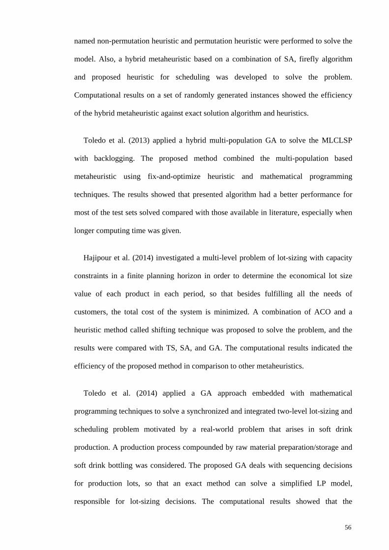
named non-permutation heuristic and permutation heuristic were performed to solve the
model. Also, a hybrid metaheuristic based on a combination of SA, firefly algorithm
and proposed heuristic for scheduling was developed to solve the problem.
Computational results on a set of randomly generated instances showed the efficiency
of the hybrid metaheuristic against exact solution algorithm and heuristics.
Toledo et al. (2013) applied a hybrid multi-population GA to solve the MLCLSP
with backlogging. The proposed method combined the multi-population based
metaheuristic using fix-and-optimize heuristic and mathematical programming
techniques. The results showed that presented algorithm had a better performance for
most of the test sets solved compared with those available in literature, especially when
longer computing time was given.
Hajipour et al. (2014) investigated a multi-level problem of lot-sizing with capacity
constraints in a finite planning horizon in order to determine the economical lot size
value of each product in each period, so that besides fulfilling all the needs of
customers, the total cost of the system is minimized. A combination of ACO and a
heuristic method called shifting technique was proposed to solve the problem, and the
results were compared with TS, SA, and GA. The computational results indicated the
efficiency of the proposed method in comparison to other metaheuristics.
Toledo et al. (2014) applied a GA approach embedded with mathematical
programming techniques to solve a synchronized and integrated two-level lot-sizing and
scheduling problem motivated by a real-world problem that arises in soft drink
production. A production process compounded by raw material preparation/storage and
soft drink bottling was considered. The proposed GA deals with sequencing decisions
for production lots, so that an exact method can solve a simplified LP model,
responsible for lot-sizing decisions. The computational results showed that the
56
evolutionary/mathematical programming approach outperforms the literature methods
in terms of production costs and run times.
Chen (2015) employed two approaches namely fix-and-optimize and VNS method
for the dynamic MLCLSP considering both without and with setup carryover.
Numerical experiments on benchmark instances showed that both applied approaches
can obtain a better solution for most instances compared with that found by the fix-and-
optimize approach proposed by Helber and Sahling (2010).
Figure 2.3 illustrates an overview of the mentioned single and multi-level lot-sizing
models.
Demand
Static
Single level production
Multi-level production
Infinite capacity
Limited capacity
EOQ
ELSP
Infinite capacity
Limited capacity
Dynamic
Single level production
Multi-level production
Infinite capacity
Limited capacity
WW Infinite capacity
Limited capacity
Micro-periods
Macro-periods
DLSPCSLPPLSP
No sequencing
Partial or complete
sequencing
CLSPLCLSDGLSP
CLSP
MLULSP
Micro-periods
Macro-periods
MLDLSPMLPLSP
MLCLSP
Figure 2.3: Classification of single and multi-level lot-sizing models
57
2.5 Multi-Facility Problems
Dantzig (1955) introduced the concept of multi-facility systems in which production
of items at one facility requires inputs from other facilities. If transportation costs are
not taken into account in multi-facility models, then the considered system is a multi-
machine or multi-stage single facility system. Due to the complexities of solving multi-
facility problems, the interdependencies between the facilities in the system are often
not taken into account, and generally multi-facility problems are solved by optimizing
the costs of each facility individually (Rizk & Martel, 2001).
Numerous studies investigating the lot-sizing and scheduling problem have
concentrated on how to effectively schedule production operations within the confines
of a single production facility. However, from the perspective of minimizing the total
cost in a supply chain, companies usually acknowledge that the cost of a product is not
only determined with the amount of factory resources used to convert the raw material
into a finished product, but also with the amount of resources used to deliver the
product to the customer. Hence, concentrating only on lot-sizing and scheduling of
production operations within plants may not be sufficient to obtain the desired low
levels in the production and logistics costs of the supply chain.
Supply chain management (SCM) problems are also connected with the solution of
lot-sizing problems in procurement-production-distribution networks. It helps to find
the optimal order, production and shipment quantities and minimize the cost including
purchasing, production and transportation flows for a set of commodities from a set of
production facilities to a set of customers. Goyal and Deshmukh (1992) reviewed
models of integrated procurement-production systems, which study combined decisions
on the optimal procurement lot size of raw material and the optimal production lot size
of finished products.
58
Since the early 1980s the integration of company-overlapping aspects in terms of
logistics has become manifest. In this regards, the term SCM was stated for the first
time by Oliver and Webber (1982). A supply chain is defined as a connected series of
activities, which is concerned with planning, coordinating and controlling functions
including procurement of materials, transformation of materials and intermediate
products into intermediate and finished products, in addition to the distribution of
finished products to customer (Ganeshan et al., 1999; Goetschalckx, 2011). SCM as
defined by Vorst (2000) is the integrated planning, coordination and control of all
material and information flows in the supply chain to deliver superior consumer value at
lower cost to the supply chain as a whole whilst satisfying requirements of other
stakeholders in the chain.
The term supply chain may also imply that only one player is involved at each stage.
In reality, a manufacturer may receive materials from several suppliers and then supply
several distributors. Thus, most supply chains are in fact considered as networks. It
might be more accurate to use the term supply network or supply web in order to
describe the structure of most supply chains (Chopra & Meindl, 2001), as shown in
Figure 2.4. Each stage in a supply chain is connected through the flow of products,
information, and funds.
59
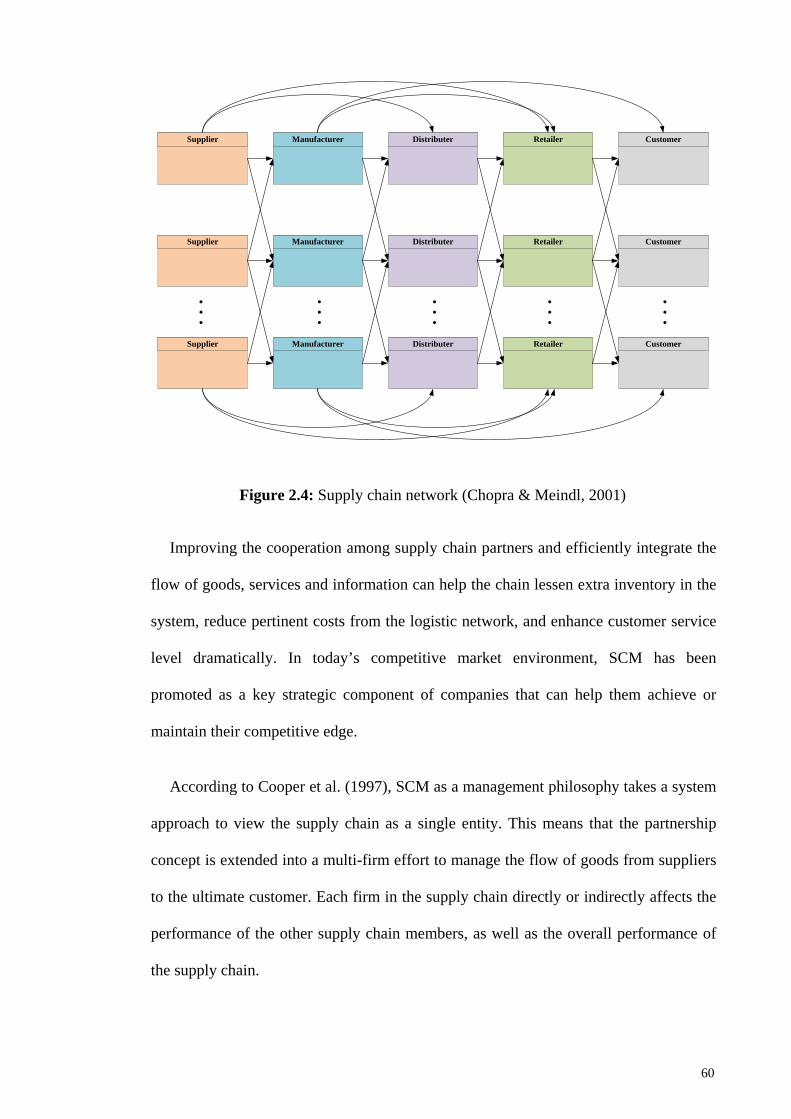
Manufacturer
Manufacturer
Manufacturer
Distributer
Distributer
Distributer
Supplier
Supplier
Supplier
Retailer
Retailer
Retailer
Customer
Customer
Customer
• • •
• • •
• • •
• • •
• • •
Figure 2.4: Supply chain network (Chopra & Meindl, 2001)
Improving the cooperation among supply chain partners and efficiently integrate the
flow of goods, services and information can help the chain lessen extra inventory in the
system, reduce pertinent costs from the logistic network, and enhance customer service
level dramatically. In today’s competitive market environment, SCM has been
promoted as a key strategic component of companies that can help them achieve or
maintain their competitive edge.
According to Cooper et al. (1997), SCM as a management philosophy takes a system
approach to view the supply chain as a single entity. This means that the partnership
concept is extended into a multi-firm effort to manage the flow of goods from suppliers
to the ultimate customer. Each firm in the supply chain directly or indirectly affects the
performance of the other supply chain members, as well as the overall performance of
the supply chain.
60
Dhaenens-Flipo (2000) presented a hierarchical heuristic which decomposes a multi-
facility multi-item production and distribution problem into several sub-problems, based
on an analogy of the vehicle routing problem, to determine the plant, production line,
and production sequence for the items in an integrated way. Dhaenens-Flipo and Finke
(2001) modeled the multi-facility, multi-item, multi-period production and distribution
problem in the form of a network flow problem and applied it successfully to a real
industrial problem.
As stated by Hwang et al. (2013), the multi-stage lot-sizing problem with production
capacities deals with a supply chain that consists of a manufacturer with stationary
production capacity and intermediaries (distribution centers or wholesalers) and a
retailer to face the deterministic demand. An optimal supply chain plan for this problem
specifies when and how many units each organization of the supply chain should
produce or transport to ultimately fulfill the demand at the retailer with the objective of
minimizing the total supply chain costs.
The importance of the coordination between production and distribution operations
have been studied in Chandra and Fisher (1994) and Fumero and Vercellis (1999). It has
been shown that integrated scheduling of production and distribution operations
perform substantially better than unsynchronized scheduling of such operations. Hence,
it is important for the companies to recognize that a reduction in total cost of the supply
chain and an increase in customer satisfaction can be realized through integrated
scheduling of production and distribution operations.
Armentano et al. (2011) studied the problem of integrating production and
distribution planning with a capacity constrained plant that produces a number of items
distributed by a fleet of homogenous vehicles to customers having known demand. Two
TS variants for this problem were proposed, one that involves construction and a short-
61
term memory, and one that incorporates a longer term memory used to integrate a path
relinking procedure to the first variant. Yan et al. (2011) integrated a production-
distribution model for a deteriorating inventory item in a two-echelon supply chain. A
procedure for determining the optimal supply chain decisions was outlined with the
objective of minimizing the total system cost.
Amorim et al. (2012) presented a multi-objective integrated production and
distribution planning for perishable products having a fixed and a loose shelf life. The
results showed that the economic benefits derived from using an integrated approach are
much dependent on the freshness level of products delivered. Pal et al. (2012) presented
a three-layer multi-item production-inventory model for multiple suppliers and
retailers. An integrated profit of the supply chain was optimized by optimal ordering lot
sizes of the raw materials.
Ben-Daya et al. (2013) examined the joint economic lot-sizing problem in the
context of a three-stage supply chain consisting of a single supplier, single manufacturer
and multi-retailers. The objective was to specify the timings and quantities of inbound
and outbound logistics for all parties involved such that the chain-wide total ordering,
setup, raw material and finished product inventory holding costs are minimized. The
derivative-free methods was employed to derive a near closed form solution for the
developed model.
Sarker et al. (2013) examined a tree-type three-echelon production-distribution
supply chain system with allowable backorder. It was attempted to improve service rate
by reducing the backorder at the retailer level. A branching search process was utilized
to obtain the solutions. Chen and Sarker (2014) utilized the ACO algorithm for solving
an integrated inventory lot-sizing and vehicle-routing model in a multi-supplier single
assembler system with just-in-time delivery. The results showed that integrated model
62
can reduce the total cost and highlighted the importance of cooperation between
suppliers and manufacturers in just-in-time production practices.
Sana et al. (2014) studied the replenishment size/production lot size problem both for
perfect and imperfect quality products in a three-layer supply chain consisting of
multiple suppliers, manufacturers and retailers. Further, the expected average profits of
suppliers, manufacturers and retailers were formulated by trading off setup costs,
purchasing costs, screening costs, production costs, inventory costs and selling prices.
In a numerical illustration, the optimal solution of the collaborating system showed a
better optimal solution than the existing related models in literature.
Yazdani et al. (2015) improved the mathematical models for the multi-factory
parallel machine problems, and compared them with the available models in both size
and computational complexities. They solved the models by the ABC algorithm and
compared them against the available algorithms on both small and large instances. It
was shown that proposed metaheuristic performed much more effectively.
2.5.1 Multi-Plant Systems
To lower the production cost and meet customer demands in time, companies have to
examine alternative solutions for their logistics network. One of these solutions can be
shifting from one plant manufacturing facility to multi-plant enterprise. Bhatnagar et al.
(1993) distinguished supply chain coordination planning into two broad categories:
coordination in terms of incorporating decisions of various functions, including
production planning, distribution, and marketing, and coordination of associating
decisions within the same operation through several echelons of the corporation. The
authors refer to the latter level of coordination as “multi-plant coordination”. Each plant
here refers to a manufacturing facility that is centered around related production
processes.
63
Shifting from single plant to multi-plant organization can bring several advantages
such as being proximate to low cost raw materials, closeness to market, flexibility in
producing various products and specialization in activities, and so forth (Maritan et al.,
2004). However, decision making in multi-plant systems has to attempt towards
integration of several manufacturing plants’ activities in such a way that they align their
tasks in direction of improving overall performance of the enterprise. Each plant’s
internal function is as important as it’s relation with other plants since each plant is a
part of the network.
Sambasivan and Schimidt (2002) provided a heuristic approach based on transfers of
production lots between the periods and the plants to solve the single stage MPCLSP.
Sambasivan and Yahya (2005) obtained better results for the problem using the LR
approach. Nascimento et al. (2010) embedded the setup carry-over to the proposed
MPCLSP, and developed a greedy randomized adaptive search procedure as well as a
path relinking intensification procedure that outperformed the LR approach proposed by
Sambasivan and Yahya (2005).
Lin and Chen (2007) presented a mathematical model for a multi-stage multi-site
production planning problem in a thin film transistor-liquid crystal display factory, and
combined two different time scales of daily and monthly time buckets. Guimarães et al.
(2012) studied a real-case scenario of a beverage industry in order to produce a long-
term plan of assigning and scheduling production lots in a multi-plant environment.
Martin et al. (1993), Chandra and Fisher (1994), and Thomas and Griffin (1996)
presented substantiations of the possible economic advantages resulting from
production-distribution integration. Pirkul and Jayaraman (1998) formulated a mixed
integer programming model for a multi-commodity, multi-plant capacitated facility
location problem, which was then solved via the LR approach to minimize the total
64
operating costs for the distribution network. Jolayemi and Olorunniwo (2004) proposed
a deterministic model for a multi-plant and multi-warehouse problem with extensible
capacities while permitting subcontracting in the case of unavailable sufficient
resources.
Park (2005) presented a heuristic solution to solve a multi-plant, multi-retailer, multi-
item problem over a multi-period horizon. The model addressed the coordination of
production and distribution planning with the aim of maximizing the total net profit.
Aghezzaf (2007) discussed the problem of production capacity and warehouse
management in a supply network in which each plant can be enabled to produce any
product type through inter-plant mold transfers.
It is proven that the single plant multi-item capacitated lot-sizing problem is NP-
Hard (Florian et al., 1980; Bitran & Yanasse, 1982), so is the respective multi-plant
version. Therefore, metaheuristic approaches can be used to efficiently tackle such
complex problems and offer good solutions within a reasonable computation time. C.
Moon et al. (2002) proposed a GA for finding high quality approximate solutions in an
integrated process planning and scheduling model for the multi-plant supply chain.
Chan et al. (2008) suggested a cooperative multiple PSO procedure to decrease the
overall tardiness in a multi-plant supply chain scenario, and attempted to resolve the
production planning and scheduling problem.
Tseng et al. (2010a, b) applied the GA and PSO to solve an integrated assembly
sequence planning and plant assignment problem where products are assembled in a
multi-plant system with the objective of minimizing the total of assembly and multi-
plant costs. Yang et al. (2010) proposed a quasi-transportation problem for multi-plant
order allocation to minimize the total cost under the capacity load constraint, and solved
it using the GA. Behnamian and Ghomi (2013) developed a heuristic algorithm and the
65
GA approach for sequencing and scheduling of distributed multi-factory production
network problem with parallel machine in order to minimize the maximum completion
time of jobs.
2.6 Conclusions
In this chapter, a detailed explanation of some of the issues related to this study, such
as single and multi-level lot-sizing problems in single facility systems, economic lot
scheduling problems, and multi-facility lot-sizing problems were given. The current
literature was reviewed and discussed. Moreover, the characteristic, aspects and
classification criteria affecting the modeling and complexity of the lot-sizing problems
were extracted from the literature and categorized.
Based on the literature review performed in this study, little attention has been
devoted to economic lot scheduling problem considering multiple setups, shelf life, and
backordering. Likewise, little attention has been paid to the multi-plant capacitated lot-
sizing problem in integrated production-distribution systems. Therefore, this study
attempts to address these shortcomings by developing comprehensive mathematical
models and solution approaches for such problems arising in reality.
66
CHAPTER 3: METHODOLOGY
3.1 Introduction
This chapter explains the methodology used in this research. The research
frameworks and a brief overview of the applied metaheuristic algorithms are also
described in this chapter.
3.2 Research Methodology
At the first step, a literature review on different aspects of lot-sizing problems in
single stage single facility and multi-stage multi-facility systems was gathered. Based
on the literature, the gaps and problems were determined. Next, the objectives and scope
of the project were identified. The first part of research focuses on modeling the multi-
item lot-sizing and scheduling problem in a single stage single facility system with a
continuous time scale, deterministic static demand and infinite time horizon which is
known as ELSP, while considering the effect of shelf life, backordering, and multiple
production frequencies for each product. The aim is to determine the optimal lot size,
production rate, production frequency, cycle time, as well as a feasible manufacturing
schedule for the family of items, and to minimize the total pertinent cost.
The second research direction emphases on lot-sizing problem in an integrated
production-distribution system. It focuses on the formulation and modeling the multi-
item capacitated lot-sizing problem in a multi-stage multi-facility system with discrete
time scale, deterministic dynamic demand and finite time horizon which is known as
MPCLSP. The objective is to find the optimal order, production, and shipment
quantities that minimize the cost of the whole supply chain.
Then, based on parameters and variables affecting the defined problems, the
objectives and scope of the study, research frameworks were created. Next,
67
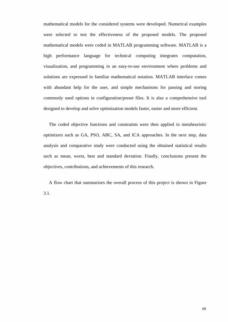
mathematical models for the considered systems were developed. Numerical examples
were selected to test the effectiveness of the proposed models. The proposed
mathematical models were coded in MATLAB programming software. MATLAB is a
high performance language for technical computing integrates computation,
visualization, and programming in an easy-to-use environment where problems and
solutions are expressed in familiar mathematical notation. MATLAB interface comes
with abundant help for the user, and simple mechanisms for passing and storing
commonly used options in configuration/preset files. It is also a comprehensive tool
designed to develop and solve optimization models faster, easier and more efficient.
The coded objective functions and constraints were then applied in metaheuristic
optimizers such as GA, PSO, ABC, SA, and ICA approaches. In the next step, data
analysis and comparative study were conducted using the obtained statistical results
such as mean, worst, best and standard deviation. Finally, conclusions present the
objectives, contributions, and achievements of this research.
A flow chart that summarizes the overall process of this project is shown in Figure
3.1.
68
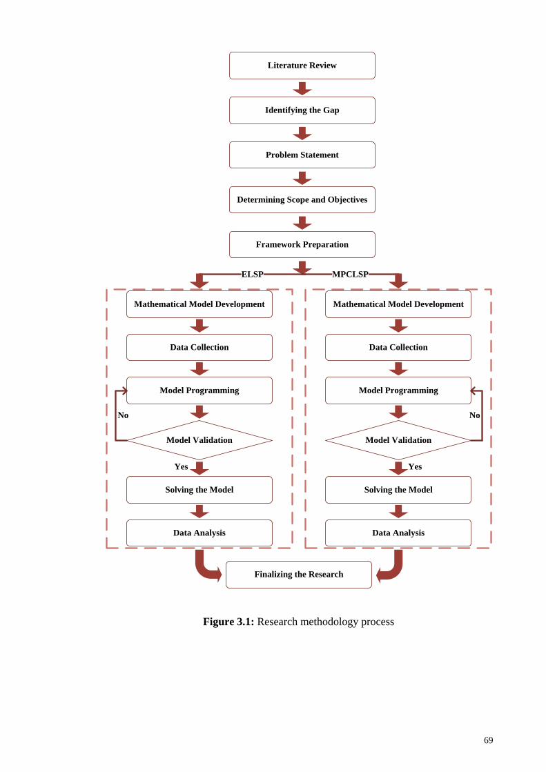
Model Validation
Literature Review
Identifying the Gap
Determining Scope and Objectives
Mathematical Model Development
Data Collection
Model Programming
Solving the Model
Yes
No
Problem Statement
Framework Preparation
Mathematical Model Development
Data Analysis
Model Validation
Data Collection
Model Programming
Solving the Model
Data Analysis
No
Yes
Finalizing the Research
MPCLSPELSP
Figure 3.1: Research methodology process
69
3.3 Research Framework
Based on the characteristics of lot-sizing problem given in Section 2.3, different
aspects of lot-sizing in both single facility and multi-facility systems are taken into
consideration. The research framework used in this project is shown in Figure 3.2.
Proposed Lot-Sizing Problem
Multi-plantSingle plant
Single stage Multi-stage
Infinite planning horizon Finite planning horizon
Continuous time period Discrete time period
Capacitated
Multi-item
Deterministic demand
Static demand Dynamic demand
Economic Lot Scheduling Problem (ELSP)
Multi-plant Capacitated Lot-Sizing Problem (MPCLSP)
Setup structure
Inventory shortage
Shelf life
Figure 3.2: Research framework
70
3.4 The Proposed ELSP
The ELSP is concerned with lot-sizing and scheduling several items in a single
production facility. The facility is such that only one item can be produced at a time and
the demand rate for each item is constant over the planning horizon. Because scarce
resources are usually shared in common by several items, the ELSP is a single stage
multi-item problem. The ELSP is a continuous time model and the planning horizon is
infinite. To solve the problem, common cycle strategy is used for all products. The
common cycle approach imposes a condition that products’ cycle times should be of
equal length, with the cycle time of a product defined in terms of the duration between
starts of two consecutive runs of the product.
Generally, the inventory systems assume implicitly unlimited shelf lives for the
stored items. However, some items can be stored in the inventory only for a certain
shelf life period which may be shorter than the production cycle time. There has been
little research on conventional ELSP models including the shelf time factor, although
many items, especially in the food industries, usually deteriorate or can be held only for
a limited lifetime. Therefore, the motivation was to devise an effective solution
approach to solve the ELSP with shelf life. Moreover, the basic ELSP does not allow
backordering. Hence, the impact of incorporating planned backorders into the system is
also investigated. Furthermore, the capacity constraint is taken into account to check
whether or not the available machining time is sufficient for setups and production.
While the cost-minimizing cycle time causes the spoilage of an item on account of
shelf life limitations, the cycle time period must be decreased to less than or equal to the
shelf life to ensure a feasible schedule. This objective may be achieved by reducing
either the total cycle time or the production rate, or by using a mix of reduced cycle time
and production rate. Consequently, the total annual costs for these three options are
71
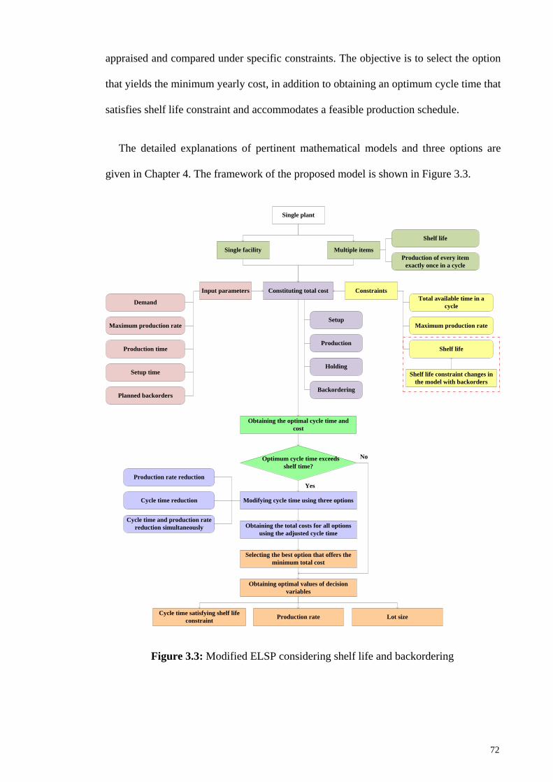
appraised and compared under specific constraints. The objective is to select the option
that yields the minimum yearly cost, in addition to obtaining an optimum cycle time that
satisfies shelf life constraint and accommodates a feasible production schedule.
The detailed explanations of pertinent mathematical models and three options are
given in Chapter 4. The framework of the proposed model is shown in Figure 3.3.
Maximum production rate Setup
Production
Setup time
Demand
Constituting total cost
Holding
Single plant
Single facility Multiple items
Shelf life
Planned backorders
ConstraintsTotal available time in a
cycle
Maximum production rate
Obtaining the optimal cycle time and cost
Production rate reduction
Cycle time reduction
Cycle time and production rate reduction simultaneously Obtaining the total costs for all options
using the adjusted cycle time
Production time
Backordering
Shelf life
Optimum cycle time exceeds shelf time?
Input parameters
Modifying cycle time using three options
Yes
No
Selecting the best option that offers the minimum total cost
Cycle time satisfying shelf life constraint Production rate
Shelf life constraint changes in the model with backorders
Production of every item exactly once in a cycle
Lot size
Obtaining optimal values of decision variables
Figure 3.3: Modified ELSP considering shelf life and backordering
72
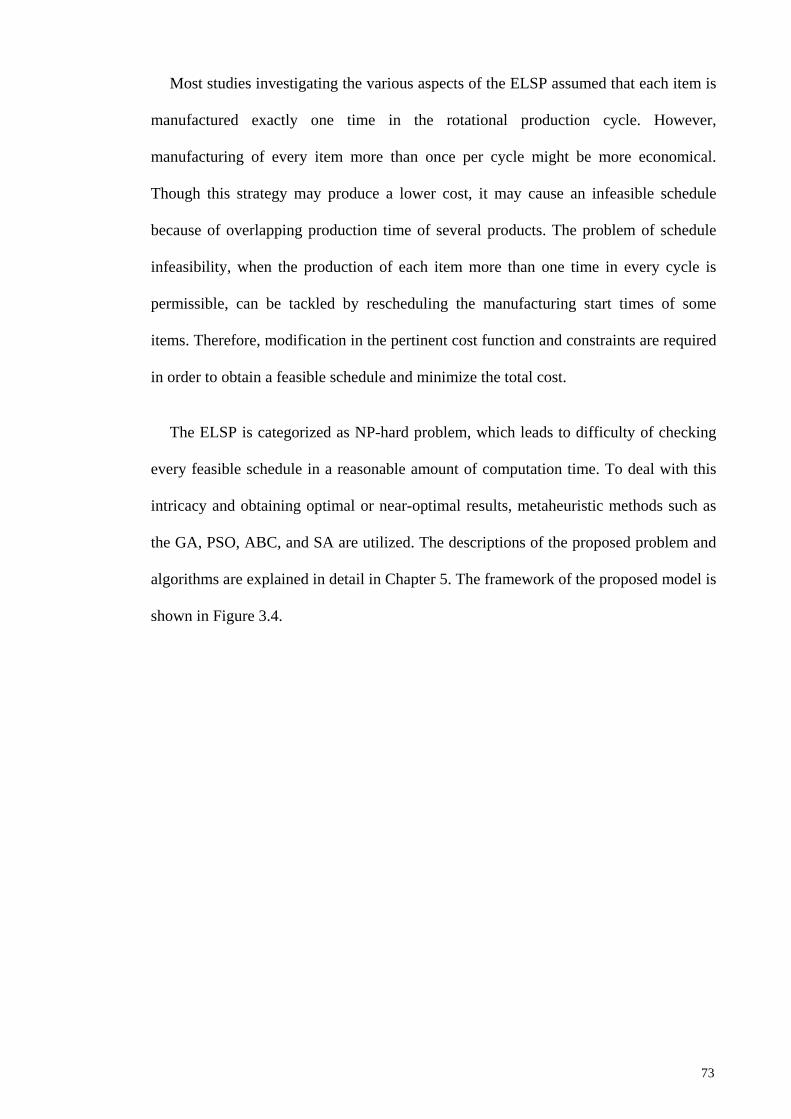
Most studies investigating the various aspects of the ELSP assumed that each item is
manufactured exactly one time in the rotational production cycle. However,
manufacturing of every item more than once per cycle might be more economical.
Though this strategy may produce a lower cost, it may cause an infeasible schedule
because of overlapping production time of several products. The problem of schedule
infeasibility, when the production of each item more than one time in every cycle is
permissible, can be tackled by rescheduling the manufacturing start times of some
items. Therefore, modification in the pertinent cost function and constraints are required
in order to obtain a feasible schedule and minimize the total cost.
The ELSP is categorized as NP-hard problem, which leads to difficulty of checking
every feasible schedule in a reasonable amount of computation time. To deal with this
intricacy and obtaining optimal or near-optimal results, metaheuristic methods such as
the GA, PSO, ABC, and SA are utilized. The descriptions of the proposed problem and
algorithms are explained in detail in Chapter 5. The framework of the proposed model is
shown in Figure 3.4.
73
Maximum production rate Setup
Production
Setup time
Demand
Constituting total cost
Holding
Single plant
Single facility Multiple itemsProduction of every item more
than once in a cycle
Constraints
Total available time in a cycle
Maximum production rate
Coding the nonlinear mixed integer ELSP model using metaheuristic algorithms
Production time
Backordering
Adjusted shelf life due to considering backorders
Input parameters
Cycle time satisfying shelf life constraint
Shelf life
Schedule feasibility
Adjustment cost in case of overlapping the production times
Genetic Algorithm
Simulated Annealing
Particle swarm optimization
Artificial Bee Colony
Calibrating metaheuristic algorithms using Taguchi method
Production frequency Production rate
Feasible manufacturing
schedule Lot size
Minimizing total cost
Obtaining optimal values of decision variables
Maximum backorder level
Figure 3.4: The proposed ELSP allowing the production of items more than once in a
cycle
74
3.5 The Proposed MPCLSP
The WW model is one of the first models for a dynamic demand problem where a
finite planning horizon is subdivided into several discrete periods and demand is given
per period and might change over time. The WW problem is considered as single level
and single item without capacity constraints. The CLSP can be considered as the
extension of the WW problem to capacity constraints and multi-item problem where its
objective is to determine the optimal lot size which minimizes production, setup, and
inventory costs.
Multi-facility systems are complex networks in the supply chain, where each facility
in the network signifies a multi-stage system. Lot-sizing problems, in this situation, are
complex due to the interdependency existing between different facilities. Therefore,
further research was carried out to examine the multi-item multi-period CLSP in a
multi-plant system. Moreover, the combination of several functions such as purchasing,
production, storage, backordering, and transportation is considered.
The nature of the multi-plant problem is closely related to the MLCLSP. In the
MLCLSP, the lot sizes need to be obtained for multi-level production inventory systems
with capacity constraints on the production facilities. In the multi-plant problem, there
is no common resource between sites, and therefore, the production is controlled
independently in each site. The MPCLSP with multiple products and time periods is
comprised of multiple production centers that manufacture all the same products and
allow transfers among the plants.
Since the MPCLSP is considered as NP-hard problem, using the exact methods may
encounter difficulties for solving medium to large size instances. Furthermore, both
deterministic and heuristic optimization methods may not be able to solve such problem
efficiently. Therefore, metaheuristic algorithms as solution methods were adopted to
75
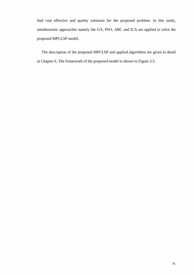
find cost effective and quality solutions for the proposed problem. In this study,
metaheuristic approaches namely the GA, PSO, ABC and ICA are applied to solve the
proposed MPCLSP model.
The description of the proposed MPCLSP and applied algorithms are given in detail
in Chapter 6. The framework of the proposed model is shown in Figure 3.5.
76
Plant 1 Plant 2 Plant j
Multiple items
Raw material 1
Raw material 2
Raw material k
Supplier 1
Supplier 2
Supplier m
• • •
Holding
Setup Setup time
Demand
Constituting total cost
Backordering
Raw material consumption
Coding the mixed integer MPCLSP using metaheuristic algorithms
Production time
Production
Ordering
Genetic Algorithms
Calibrating metaheuristic algorithms using Taguchi method
Backorder amount
Resource consumption
Total available time
Purchasing
Transportation
Supplier capacity
Vehicle capacity
• • •
• • •
Storage capacity
Selling price
Inventory balance
Setup / ordering charging
Available production time
Raw material purchasing
Resource limitation
Transportation limitation
Vehicle quantity
Inventory storage
Backorder balance
ConstraintsInput parameters
Rejection percentage
Performance percentage
Productivity percentage
Imperialist Competitive Algorithm
Particle swarm optimization
Artificial Bee Colony
Minimizing total cost
Obtaining optimal values of decision variables
Inter-plant transferred quantityOrder quantity
Transportation amount to distribution centers
Inventory level of raw material
Inventory level of products
Production quantity
Number of vehicles
Figure 3.5: The proposed multi-period multi-item MPCLSP
77
3.6 Solution Methods
Metaheuristic algorithms have been extensively used in solving complex
optimization problems in various fields of scientific and engineering disciplines, since
classical and traditional techniques may not efficiently find the global optimum
solutions.
In the literature, diverse classes of metaheuristic algorithms inspired by various
models of biological species or physical phenomena have been developed for solving
complex optimization problems. A common feature behind such metaheuristic
algorithms is that they go through three general phases: initiate, neighborhood search,
and terminate. That is, these algorithms start from one or a population of initial
incumbent solution(s) and then iteratively search for better solutions from the
neighborhood of the incumbent solution(s) by following specific mechanisms until the
terminating condition is met. The specific mechanisms of these algorithms are in fact
types of NS techniques in analogy with natural phenomena such as biology evolution,
biological behaviors, metal annealing processes, etc.
Since the capacitated lot-sizing and scheduling problem is considered as NP-hard in
nature, a number of widely used metaheuristic methods are selected to solve the
proposed mathematical problems in this research. The overall procedures of the applied
algorithms are explained in the following subsections.
3.6.1 Genetic Algorithm
The GA is considered as an evolutionary algorithm and a population-based method
that attempts to finds the optimal or near-optimal solutions through conducting a
random search. Fundamental of the GA was primarily instated by Holland (1975). The
GA method has been effectively used for solving continuous and discrete combinatorial
problems (Mitchell, 1996). Simplicity and capability of finding quick reasonable
78
solutions for intricate searching and optimization problems have brought about a
growing interest over the GA. This algorithm is based upon “survival of the fittest”
principles by Darwin Theory of Evolution and simulates the process of natural
evolution.
A GA contains a set of individuals that constitute the population. Every individual in
the population is represented by a particular chromosome which refers to a plausible
solution to the existing problem. Throughout consecutive repetitions, called generations,
the chromosomes evolve through reproduction process. During each generation, the
fitness value of each chromosome is evaluated. Upon the selection of some
chromosomes from the existing generation as parents, offspring will be produced by
either crossover or mutation operators. The algorithm will be stopped when a
termination condition is reached. The overall flowchart of the GA approach is shown in
Figure 3.6.
79
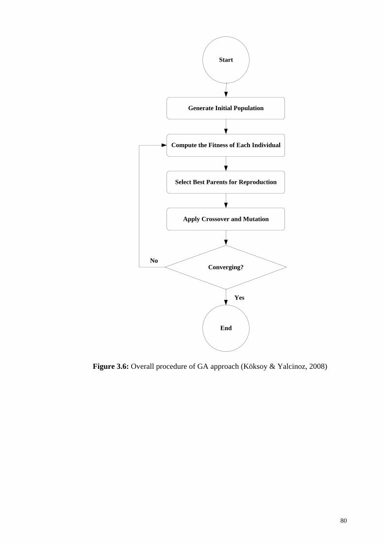
Start
Generate Initial Population
Compute the Fitness of Each Individual
Select Best Parents for Reproduction
Apply Crossover and Mutation
End
Converging?
Yes
No
Figure 3.6: Overall procedure of GA approach (Köksoy & Yalcinoz, 2008)
80
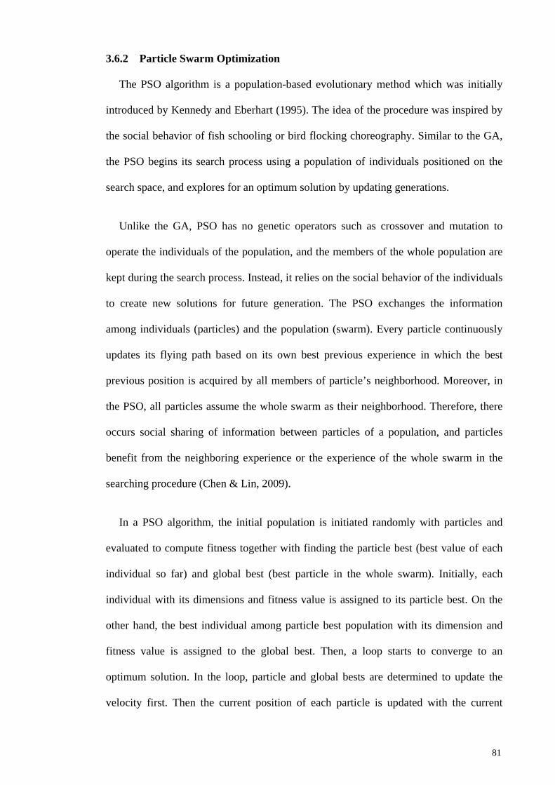
3.6.2 Particle Swarm Optimization
The PSO algorithm is a population-based evolutionary method which was initially
introduced by Kennedy and Eberhart (1995). The idea of the procedure was inspired by
the social behavior of fish schooling or bird flocking choreography. Similar to the GA,
the PSO begins its search process using a population of individuals positioned on the
search space, and explores for an optimum solution by updating generations.
Unlike the GA, PSO has no genetic operators such as crossover and mutation to
operate the individuals of the population, and the members of the whole population are
kept during the search process. Instead, it relies on the social behavior of the individuals
to create new solutions for future generation. The PSO exchanges the information
among individuals (particles) and the population (swarm). Every particle continuously
updates its flying path based on its own best previous experience in which the best
previous position is acquired by all members of particle’s neighborhood. Moreover, in
the PSO, all particles assume the whole swarm as their neighborhood. Therefore, there
occurs social sharing of information between particles of a population, and particles
benefit from the neighboring experience or the experience of the whole swarm in the
searching procedure (Chen & Lin, 2009).
In a PSO algorithm, the initial population is initiated randomly with particles and
evaluated to compute fitness together with finding the particle best (best value of each
individual so far) and global best (best particle in the whole swarm). Initially, each
individual with its dimensions and fitness value is assigned to its particle best. On the
other hand, the best individual among particle best population with its dimension and
fitness value is assigned to the global best. Then, a loop starts to converge to an
optimum solution. In the loop, particle and global bests are determined to update the
velocity first. Then the current position of each particle is updated with the current
81
velocity. Evaluation is again performed to compute the fitness of the particles in the
swarm. This loop is terminated with a stopping criterion predetermined in advance. The
overall flowchart of the PSO algorithm is shown in Figure 3.7.
Setup Parameters
Initial Population
Evaluate Fitness
Update Velocity
Move Positions of Particles
Check TerminationCondition
Start
Check Feasibility of Solutions
Evaluate Fitness
End
Yes
No
Figure 3.7: Overall procedure of PSO algorithm (Tseng et al., 2010b)
82
3.6.3 Artificial Bee Colony
The ABC algorithm was proposed by Karaboga (2005) which mimics the intelligent
behavior of the honey bee swarm in foraging foods. It is a population-based search
algorithm suitable for multi-variable and continuous multi-modal optimization
problems. The ABC algorithm includes four main components, namely food sources,
employed bees, onlooker bees, and scout bees.
A food source position represents a possible solution to the problem to be optimized.
The amount of nectar of a food source corresponds to the quality of the solution
represented by that food source (Karaboga & Basturk, 2008). A bee which has found a
food source to exploit is called an employed bee. Onlookers are those waiting in the
hive to receive the information about the food sources from the employed bees. An
onlooker bee appraises the food information obtained from employed bees, and chooses
a food source based on the probability related to their nectars’ amounts. For this purpose
the greedy selection method is applied, so that if the amount of nectar of a new source is
higher than the previous one in their memory, onlooker bees update the new position
and forget the previous one.
Scouts are the bees which are randomly searching for new food sources around the
hive. The employed bee whose its food source has been exhausted becomes a scout. In
the basic ABC process, in every cycle at most one scout goes outside for exploring a
new food source. After the new position is specified, a new algorithm cycle begins.
After each cycle, the finest solution will be memorized. The same process iterates until
the termination condition is reached. The overall flowchart of the ABC algorithm is
shown in Figure 3.8.
83
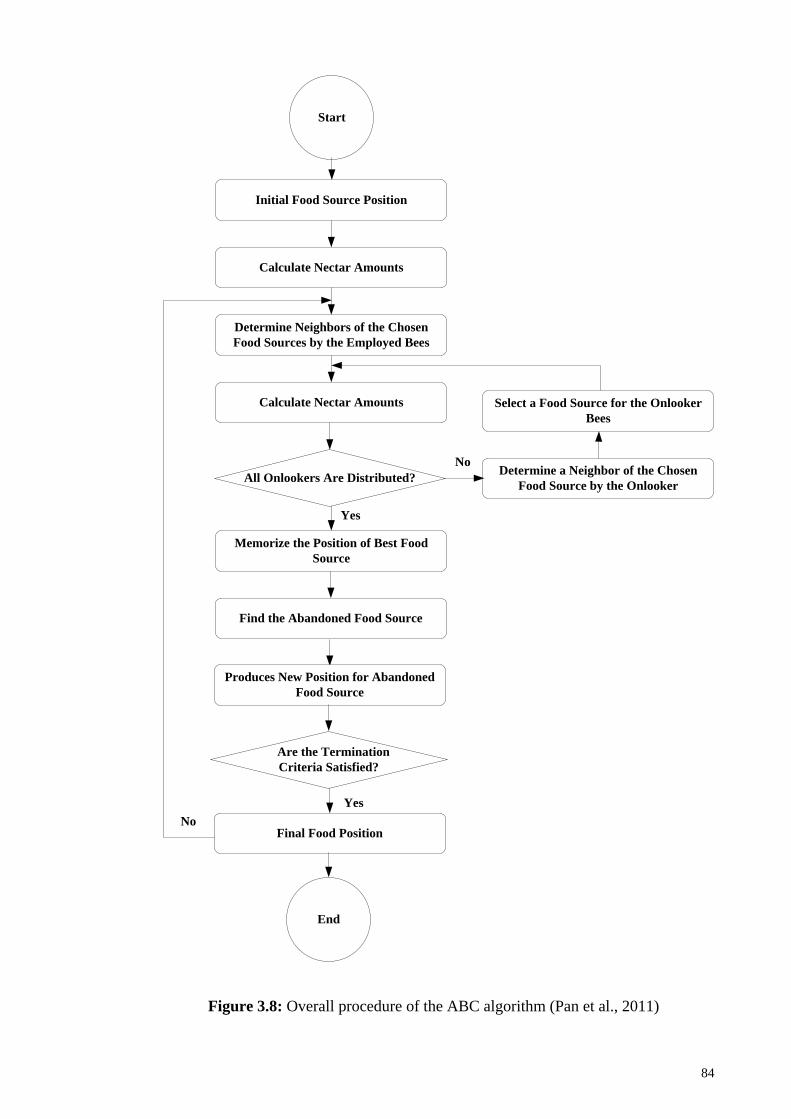
Initial Food Source Position
Calculate Nectar Amounts
Determine Neighbors of the Chosen Food Sources by the Employed Bees
Calculate Nectar Amounts
Memorize the Position of Best Food Source
Find the Abandoned Food Source
Produces New Position for Abandoned Food Source
Final Food Position
Select a Food Source for the Onlooker Bees
Determine a Neighbor of the Chosen Food Source by the Onlooker
Yes
No
No
Yes
Start
Are the Termination Criteria Satisfied?
End
All Onlookers Are Distributed?
Figure 3.8: Overall procedure of the ABC algorithm (Pan et al., 2011)
84
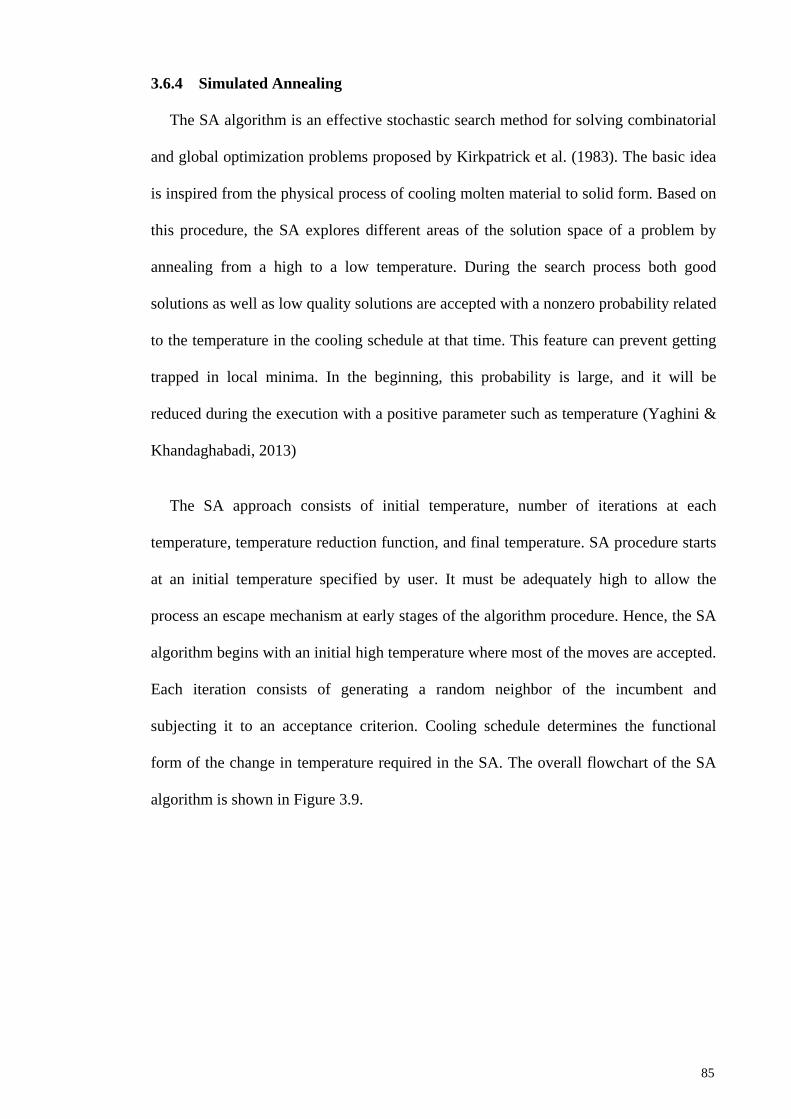
3.6.4 Simulated Annealing
The SA algorithm is an effective stochastic search method for solving combinatorial
and global optimization problems proposed by Kirkpatrick et al. (1983). The basic idea
is inspired from the physical process of cooling molten material to solid form. Based on
this procedure, the SA explores different areas of the solution space of a problem by
annealing from a high to a low temperature. During the search process both good
solutions as well as low quality solutions are accepted with a nonzero probability related
to the temperature in the cooling schedule at that time. This feature can prevent getting
trapped in local minima. In the beginning, this probability is large, and it will be
reduced during the execution with a positive parameter such as temperature (Yaghini &
Khandaghabadi, 2013)
The SA approach consists of initial temperature, number of iterations at each
temperature, temperature reduction function, and final temperature. SA procedure starts
at an initial temperature specified by user. It must be adequately high to allow the
process an escape mechanism at early stages of the algorithm procedure. Hence, the SA
algorithm begins with an initial high temperature where most of the moves are accepted.
Each iteration consists of generating a random neighbor of the incumbent and
subjecting it to an acceptance criterion. Cooling schedule determines the functional
form of the change in temperature required in the SA. The overall flowchart of the SA
algorithm is shown in Figure 3.9.
85
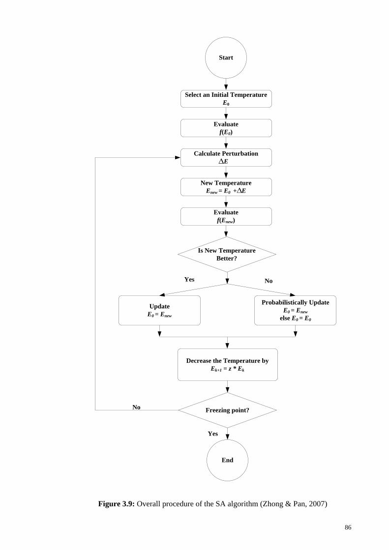
Select an Initial Temperature E0
Evaluatef(E0)
Calculate PerturbationE
New Temperature Enew = E0 + E
Evaluatef(Enew)
Is New Temperature Better?
∆
Probabilistically UpdateE0 = Enew
else E0 = E0
UpdateE0 = Enew
Decrease the Temperature byEk+1 = z * Ek
∆
Yes No
Start
Freezing point?
End
Yes
No
Figure 3.9: Overall procedure of the SA algorithm (Zhong & Pan, 2007)
86
3.6.5 Imperialist Competitive Algorithm
The ICA approach is a type of population-based algorithms that is inspired by
imperialist competition (Atashpaz-Gargari & Lucas, 2007). The ICA defines the term
‘country’ (Parsapoor & Bilstrup, 2013) to encode the optimization problems. An initial
population of the ICA is a set of countries, where each country is a vector of the
optimization parameters. The population is classified into two groups: the colonies and
the imperialists. The countries that have the higher power are considered as the
imperialists and start to take possession of the countries with the lower power, which
are stated as colonies. In this way, each imperialist creates its empire. The steps of
creating empires are explained as follow:
i. First, the cost of each country (it is equivalent to the fitness function in the GA) is
calculated. The countries with minimum values of cost (in minimization problems)
are chosen as the imperialists.
ii. The imperialists take procession of the colonies based on the normalized power.
iii. The normalized cost for each imperialist is calculated.
iv. After forming the empires, the movement of colonies toward the imperialists is
started (assimilation operator). If a colony reaches to a higher power than its
imperialist, the position of the colony and its imperialist must be exchanged
(evolution operator).
v. Finally, the imperialists start a competition to take the possession of the weakest
colonies of the weakest empires. During the competition, the weakest colony from
the weakest empire is picked and joined to the most powerful imperialist. The
weakest empires, whose colonies are joined to other empires, will be eliminated.
The algorithm is converged to a global optimum when there is one empire.
87
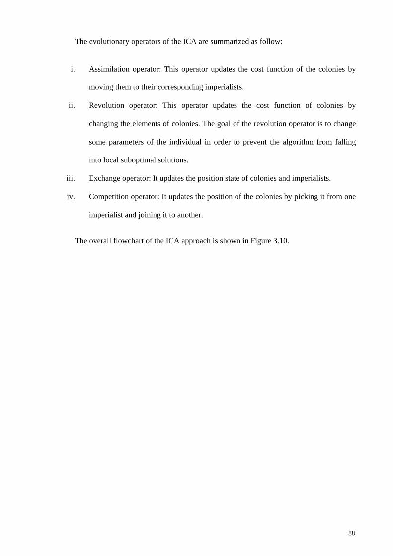
The evolutionary operators of the ICA are summarized as follow:
i. Assimilation operator: This operator updates the cost function of the colonies by
moving them to their corresponding imperialists.
ii. Revolution operator: This operator updates the cost function of colonies by
changing the elements of colonies. The goal of the revolution operator is to change
some parameters of the individual in order to prevent the algorithm from falling
into local suboptimal solutions.
iii. Exchange operator: It updates the position state of colonies and imperialists.
iv. Competition operator: It updates the position of the colonies by picking it from one
imperialist and joining it to another.
The overall flowchart of the ICA approach is shown in Figure 3.10.
88
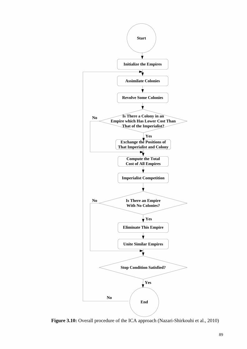
Initialize the Empires
Assimilate Colonies
Revolve Some Colonies
Exchange the Positions of That Imperialist and Colony
Compute the TotalCost of All Empires
Is There an EmpireWith No Colonies?
Eliminate This Empire
Stop Condition Satisfied?
Imperialist Competition
Yes
No
Yes
Unite Similar Empires
End
Yes
Start
No
No
Is There a Colony in anEmpire which Has Lower Cost Than
That of the Imperialist?
Figure 3.10: Overall procedure of the ICA approach (Nazari-Shirkouhi et al., 2010)
89
3.7 Conclusions
In this chapter, the methodology used in the study was explained and illustrated by a
flowchart. The proposed research frameworks were also demonstrated. The proposed
frameworks were divided into three main phases, namely the ELSP considering shelf
life and backordering, the ELSP allowing the production of items more than once in a
cycle, and MPCLSP in an integrated production-distribution system.
A brief overview of the mechanisms of a number of metaheuristic approaches,
namely GA, PSO, ABC, SA, and ICA was also presented, which are used to deal with
the intricacy of the proposed models and obtain near-optimal to optimal solutions in a
reasonable computation time.
90
CHAPTER 4: OPTIMAL CYCLE TIME FOR PRODUCTION-INVENTORY
SYSTEMS CONSIDERING SHELF LIFE AND BACKORDERING
4.1 Introduction
This chapter investigates a manufacturing system considering the production of a
family of items in a single facility environment. Total backordering is allowed for any
of the products, and each item has a specified shelf life. Nevertheless, in existing
literature, when backordering is included, the shelf life constraint variation is not taken
into account. While the cost-minimizing cycle time causes the spoilage of an item due
to shelf life limitation, the cycle time period must be decreased to less than or equal to
the shelf life to ensure a feasible schedule. Therefore, three options namely “cycle time
reduction,” “production rate reduction” and “cycle time and production rate reduction
simultaneously” are examined in order to obtain an optimum cycle time that satisfies the
shelf life constraint. The cost functions for three options are also modified because of
the shelf life constraint adjustment after considering backordering.
The rest of this chapter is organized as follows: Section 4.2 presents a detailed
discussion on the cost functions and problem constraints by examining the three
mentioned options. Section 4.3 demonstrates numerical examples and reports the
obtained results. Finally, conclusions are provided in Section 4.4.
4.2 Problem Description and Mathematical Formulations
In this study, a single machine is considered that produces N types of items in
manufacturing cycle time of T. Total backordering is permitted for each item while each
product has a certain shelf life. The total cost, including setup, holding, production, and
shortage cost are expressed through mathematical formulation for the cycle time T.
Using the total cost function under the given constraints, the optimal cycle time and cost
are obtained while disallowing the shelf life constraint.
91
For the case where the optimum cycle time T causes spoilage of an item, three
options are investigated: 1) production rate reduction, 2) cycle time reduction, and 3)
cycle time and production rate reduction simultaneously. Next, the adjusted cycle times
for the three options are estimated by considering the shelf life constraint. Using the
adjusted cycle times, the total costs for all options are found and compared in order to
select the best option that offers the minimum total cost.
The mathematical model studied throughout this chapter is based on the following
assumptions and notations:
(a) Assumptions
i. There is a constant demand rate for each product.
ii. The production rate for each product is finite.
iii. The facility can produce only one item at a time.
iv. All items are produced on each manufacturing cycle.
v. Stock is used on a first-in-first-out basis.
(b) Notations
For the entire family:
N Total number of items
T Production cycle time (years)
TO Optimum production cycle time (years)
O Production cost for operating the machine (including setup times) (dollars/year)
C Total cost (dollars/year)
For item i (i = 1, 2, … , N):
di Demand for item i (units/year)
pi Production rate for item i (units/year)
92
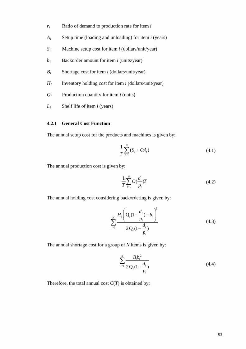
ri Ratio of demand to production rate for item i
Ai Setup time (loading and unloading) for item i (years)
Si Machine setup cost for item i (dollars/unit/year)
bi Backorder amount for item i (units/year)
Bi Shortage cost for item i (dollars/unit/year)
Hi Inventory holding cost for item i (dollars/unit/year)
Qi Production quantity for item i (units)
Li Shelf life of item i (years)
4.2.1 General Cost Function
The annual setup cost for the products and machines is given by:
1
1 ( )N
i ii
S OAT =
+∑ (4.1)
The annual production cost is given by:
1
1 ( )N
i
i i
dO TT p=
∑ (4.2)
The annual holding cost considering backordering is given by:
2
1
Q (1 )
2Q (1 )
ii i iN
i
iii
i
dH bp
dp
=
− −
−∑ (4.3)
The annual shortage cost for a group of N items is given by:
2
1 2Q (1 )
Ni i
iii
i
B bdp
= −∑
(4.4)
Therefore, the total annual cost C(T) is obtained by:
93
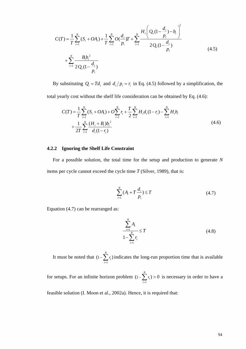
2
1 1 1
2
1
Q (1 )1 1( ) ( ) ( )
2Q (1 )
2Q (1 )
ii i iN N N
iii i
ii i iii
i
Ni i
iii
i
dH bpdC T S OA O T dT T p
p
B bdp
= = =
=
− −
= + + +−
+−
∑ ∑ ∑
∑
(4.5)
By substituting i iQ Td= and i i id p r= in Eq. (4.5) followed by a simplification, the
total yearly cost without the shelf life consideration can be obtained by Eq. (4.6):
1 1 1 12
1
1( ) ( ) (1 )2
( )12 (1 )
N N N N
i i i i i i i ii i i i
Ni i i
i i i
TC T S OA O r H d r H bT
H B bT d r
= = = =
=
= + + + − −
++
−
∑ ∑ ∑ ∑
∑ (4.6)
4.2.2 Ignoring the Shelf Life Constraint
For a possible solution, the total time for the setup and production to generate N
items per cycle cannot exceed the cycle time T (Silver, 1989), that is:
1
( )N
ii
i i
dA T Tp=
+ ≤∑ (4.7)
Equation (4.7) can be rearranged as:
1
11
N
ii
N
ii
AT
r
=
=
≤−
∑
∑ (4.8)
It must be noted that 1
1( )N
ii
r=
− ∑ indicates the long-run proportion time that is available
for setups. For an infinite horizon problem 1
1( ) 0N
ii
r=
− >∑ is necessary in order to have a
feasible solution (I. Moon et al., 2002a). Hence, it is required that:
94
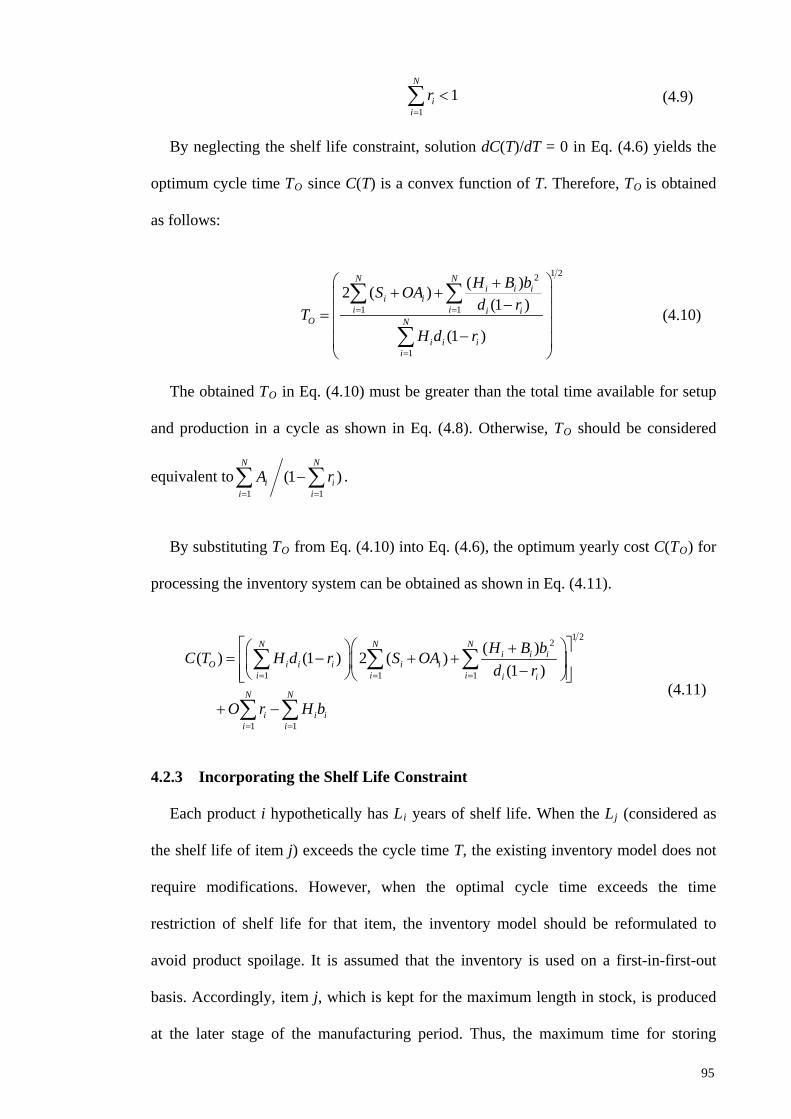
1
1N
ii
r=
<∑ (4.9)
By neglecting the shelf life constraint, solution dC(T)/dT = 0 in Eq. (4.6) yields the
optimum cycle time TO since C(T) is a convex function of T. Therefore, TO is obtained
as follows:
1 22
1 1
1
( )2 ( )(1 )
(1 )
N Ni i i
i ii i i i
O N
i i ii
H B bS OAd rT
H d r
= =
=
++ + − =
−
∑ ∑
∑ (4.10)
The obtained TO in Eq. (4.10) must be greater than the total time available for setup
and production in a cycle as shown in Eq. (4.8). Otherwise, TO should be considered
equivalent to1 1
(1 )N N
i ii i
A r= =
−∑ ∑ .
By substituting TO from Eq. (4.10) into Eq. (4.6), the optimum yearly cost C(TO) for
processing the inventory system can be obtained as shown in Eq. (4.11).
1 22
1 1 1
1 1
( )( ) (1 ) 2 ( )(1 )
N N Ni i i
O i i i i ii i i i i
N N
i i ii i
H B bC T H d r S OAd r
O r H b
= = =
= =
+ = − + + −
+ −
∑ ∑ ∑
∑ ∑ (4.11)
4.2.3 Incorporating the Shelf Life Constraint
Each product i hypothetically has Li years of shelf life. When the Lj (considered as
the shelf life of item j) exceeds the cycle time T, the existing inventory model does not
require modifications. However, when the optimal cycle time exceeds the time
restriction of shelf life for that item, the inventory model should be reformulated to
avoid product spoilage. It is assumed that the inventory is used on a first-in-first-out
basis. Accordingly, item j, which is kept for the maximum length in stock, is produced
at the later stage of the manufacturing period. Thus, the maximum time for storing
95
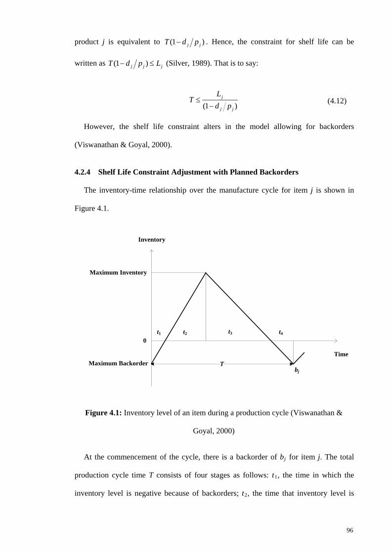
product j is equivalent to (1 )j jT d p− . Hence, the constraint for shelf life can be
written as (1 )j j jT d p L− ≤ (Silver, 1989). That is to say:
(1 )j
j j
LT
d p≤
− (4.12)
However, the shelf life constraint alters in the model allowing for backorders
(Viswanathan & Goyal, 2000).
4.2.4 Shelf Life Constraint Adjustment with Planned Backorders
The inventory-time relationship over the manufacture cycle for item j is shown in
Figure 4.1.
Maximum Inventory
0
TimeMaximum Backorder
bj
t1 t2 t3 t4
T
Inventory
Figure 4.1: Inventory level of an item during a production cycle (Viswanathan &
Goyal, 2000)
At the commencement of the cycle, there is a backorder of bj for item j. The total
production cycle time T consists of four stages as follows: t1, the time in which the
inventory level is negative because of backorders; t2, the time that inventory level is
96
greater than zero and increasing; t3, the time which production has ended and the
inventory level is being decreased from the maximum level to zero; and t4, the time that
inventory level lowers from zero to the total backorder at the end of the cycle. Since the
demand rate for item j is denoted as dj and the production rate is denoted as pj, we have:
4j
j
bt
d= (4.13)
1 1j j jt d b t p+ = (4.14)
1 4 (1 )j
j j j
bt t
d d p+ =
− (4.15)
since:
1 2j
j
dt t T
p+ = (4.16)
and:
1 2 3 4t t t t T+ + + = (4.17)
Hence:
2 (1 )j j
j j j j
d bt T
p p d p= −
− (4.18)
and:
3 (1 ) jj j
j
bt T d p
d= − − (4.19)
The optimum bj is obtained by equating the first derivative of the total cost given in
Eq. (4.6) to zero, which gives:
97
(1 )( )
jj j j j
j j
Hb d T d p
H B= −
+ (4.20)
The maximum amount of time that an item stays in inventory is equal to t3.
Therefore, the shelf life constraint for item j becomes as Eq. (4.21).
3 (1 ) jj j j
j
bt T d p L
d= − − ≤ (4.21)
Which it can be re-written as:
(1 )
( )(1 )
jj j j
j jj j j
j
Hd T d p
H BT d p L
d
−+
− − ≤ (4.22)
It can be rearranged again as:
( )
(1 )
j jj
j
j j
H BL
BT
d p
+
≤−
(4.23)
In Eq. (4.23), the variable parameters are the production rate pj and cycle time T
which can be adjusted in order to satisfy the shelf life constraint. Next, the three options
are examined to adjust these variables individually and simultaneously. Moreover, the
available related inventory models are modified in order to find a feasible solution
following shelf life adjustment.
4.2.5 Option 1: Production Rate Reduction
The reduction of production rate lowers the average inventory and thus items in the
inventory are used up at a quicker rate. Hence, products are not kept longer than their
shelf life duration.
In this option, the production rate p is adjusted to satisfy the constraint for shelf life
along with the cycle time T which is considered as a fixed measure (T is the same as the
optimal cycle time obtained by Eq. (4.10)) as illustrated in Figure 4.2.
98
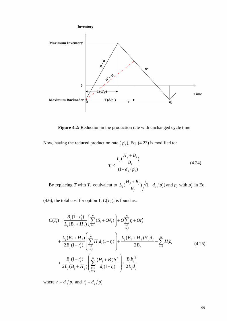
Maximum Inventory
0
TimeMaximum Backorder
p – d
p' – d
b
d
T(d/p)
T(d/p') T
Inventory
Figure 4.2: Reduction in the production rate with unchanged cycle time
Now, having the reduced production rate ( jp′ ), Eq. (4.23) is modified to:
1
( )
(1 )
j jj
j
j j
H BL
BT
d p
+
≤′−
(4.24)
By replacing T with T1 equivalent to ( ) (1 )j jj j j
j
H BL d p
B+
′− and pj with jp′ in Eq.
(4.6), the total cost for option 1, C(T1), is found as:
11 1
1 1
22
1
(1 )( ) ( )
( )
( ) ( )(1 )
2 (1 ) 2
(1 ) ( )2 ( ) (1 ) 2
N Nj j
i i i ji ij j j
i j
N Nj j j j j j j j
i i i i ii ij j ji j
Nj j j ji i i
ij j j i i ji j
B rC T S OA O r Or
L B H
L B H L B H H dH d r H b
B r B
B r B bH B bL B H d r L
= =≠
= =≠
=≠
′− ′= + + + +
+ + + − + − ′−
′− + + + + −
∑ ∑
∑ ∑
∑jd
(4.25)
where i i ir d p= and j j jr d p′ ′=
99
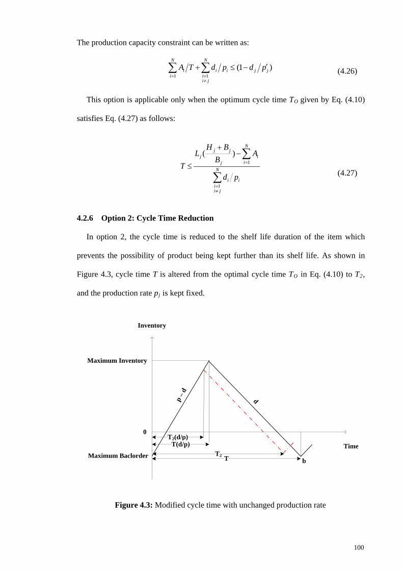
The production capacity constraint can be written as:
1 1
(1 )N N
i i i j ji i
i j
A T d p d p= =
≠
′+ ≤ −∑ ∑ (4.26)
This option is applicable only when the optimum cycle time TO given by Eq. (4.10)
satisfies Eq. (4.27) as follows:
1
1
( )N
j jj i
ijN
i iii j
H BL A
BT
d p
=
=≠
+−
≤∑
∑
(4.27)
4.2.6 Option 2: Cycle Time Reduction
In option 2, the cycle time is reduced to the shelf life duration of the item which
prevents the possibility of product being kept further than its shelf life. As shown in
Figure 4.3, cycle time T is altered from the optimal cycle time TO in Eq. (4.10) to T2,
and the production rate pj is kept fixed.
Maximum Inventory
0
TimeMaximum Baclorder
p – d
b
d
T2
T2(d/p)T(d/p)
T
Inventory
Figure 4.3: Modified cycle time with unchanged production rate
100
The adjusted cycle time T2 is given by:
2
( )
(1 )
j jj
j
j j
H BL
BT
d p
+
=−
(4.28)
Subject to:
12
1(1 )
N
ii
N
ii
AT
r
=
=
≤−
∑
∑ (4.29)
By replacing the new cycle time, T2, from Eq. (4.28) into Eq. (4.6), the total cost for
option 2, C(T2), can be obtained as:
21 1
1 1
2
1
(1 )( ) ( )
( )
( )(1 )
2 (1 )
(1 ) ( )2 ( ) (1 )
N Nj j
i i ii ij j j
N Nj j j
i i i i ii ij j
Nj j i i i
ij j j i i
B rC T S OA O r
L B H
L B HH d r H b
B r
B r H B bL B H d r
= =
= =
=
− = + + +
+ + − − −
− ++ + −
∑ ∑
∑ ∑
∑
(4.30)
The total costs in Eqs. (4.25) and (4.30) must be compared in order to identify which
option (1 or 2) is more cost-effective. Therefore, the difference in the total yearly
inventory costs for the two options is given by 1 2( ) ( )C C T C T∆ = − , which can be
calculated as follows:
( )
1
1
2
1
( )( ) (S )
( )
( )(1 )
2 (1 )(1 )
( )2 ( ) (1 )
Nj j j
j j i iij j j
Nj j j j j
i i iij j ji j
Nj i i i
j jij j j i ii j
B r rC O r r OA
L B H
L B H r rH d r
B r r
B H B b r rL B H d r
=
=≠
=≠
′− ′∆ = − + + +
′+ −+ − ′− −
+ ′+ −+ −
∑
∑
∑
(4.31)
A positive value for ∆C implies that the cost of option 1 is greater than option 2.
Hence, it is efficient to use option 2.
101
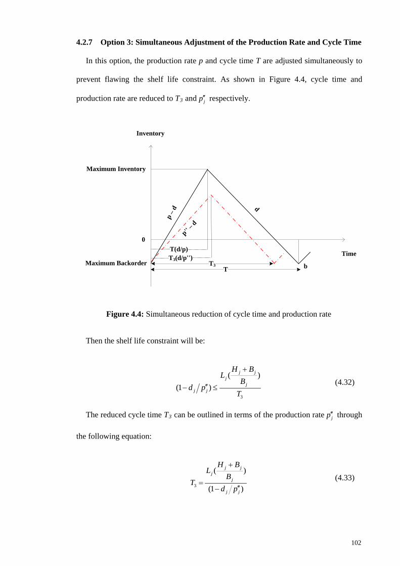
4.2.7 Option 3: Simultaneous Adjustment of the Production Rate and Cycle Time
In this option, the production rate p and cycle time T are adjusted simultaneously to
prevent flawing the shelf life constraint. As shown in Figure 4.4, cycle time and
production rate are reduced to T3 and jp′′ respectively.
Maximum Inventory
0
TimeMaximum Backorder
p – dp'' –
d
b
d
T3
T(d/p)
T
T3(d/p'')
Inventory
Figure 4.4: Simultaneous reduction of cycle time and production rate
Then the shelf life constraint will be:
3
( )(1 )
j jj
jj j
H BL
Bd p
T
+
′′− ≤ (4.32)
The reduced cycle time T3 can be outlined in terms of the production rate jp′′ through
the following equation:
3
( )
(1 )
j jj
j
j j
H BL
BT
d p
+
=′′−
(4.33)
102
Equation (4.33) is equivalent to:
3
( )1
j jj
jj
H BL
Br
T
+
′′= − (4.34)
where j j jr d p′′ ′′=
Subsequently, the capacity constraint can be written as:
3
1 1
3
(1 )
N N
i ii i
i jj j
A T r
d pT
= =≠
+
′′≤ −
∑ ∑
(4.35)
The constraints represented in Eqs. (4.32) and (4.35) are feasible only when:
31 1
( )N N
j ji i i j
i i ji j
H BA T d p L
B= =≠
++ ≤∑ ∑ (4.36)
or:
1
3
1
( )N
j jj i
ijN
i iii j
H BL A
BT
d p
=
=≠
+−
≤∑
∑ (4.37)
By changing T in Eq. (4.6) to T3 in Eq. (4.33), the total cost is given as:
33
1 1 13
23
1 13
2
3
1( ) (S ) (1 )2
( )1(1 )2 2 (1 )
( )12 (1 )
N N N
i i i j i i ii i i
i j i j
N Ni i i
j j j i ii i i i
i j
j j j
j j
TC T OA O r Or H d rT
T H B bH d r H bT d r
H B bT d r
= = =≠ ≠
= =≠
′′= + + + + −
+′′+ − − +−
++ ×
′′−
∑ ∑ ∑
∑ ∑ (4.38)
103
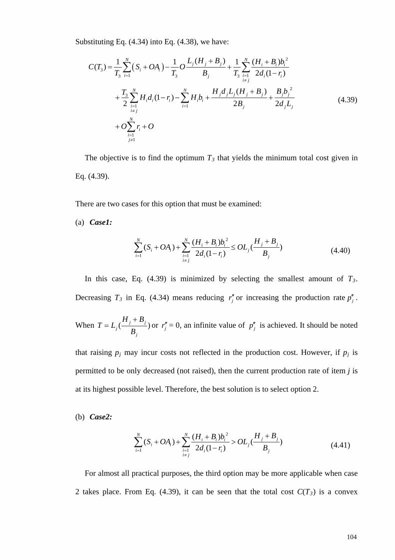
Substituting Eq. (4.34) into Eq. (4.38), we have:
( )2
31 13 3 3
23
1 1
11
( ) ( )1 1 1( )2 (1 )
( )(1 )
2 2 2
N Nj j j i i i
i ii ij i i
i j
N Nj j j j j j j
i i i i ii i j j ji j
N
iij
L H B H B bC T S OA OT T B T d r
H d L H B B bT H d r H bB d L
O r O
= =≠
= =≠
=≠
+ += + − +
−
++ − − + +
+ +
∑ ∑
∑ ∑
∑
(4.39)
The objective is to find the optimum T3 that yields the minimum total cost given in
Eq. (4.39).
There are two cases for this option that must be examined:
(a) Case1:
2
1 1
( )( ) ( )2 (1 )
N Nj ji i i
i i ji i i i j
i j
H BH B bS OA OLd r B= =
≠
+++ + ≤
−∑ ∑ (4.40)
In this case, Eq. (4.39) is minimized by selecting the smallest amount of T3.
Decreasing T3 in Eq. (4.34) means reducing jr′′or increasing the production rate jp′′ .
When ( )j jj
j
H BT L
B+
= or jr′′= 0, an infinite value of jp′′ is achieved. It should be noted
that raising pj may incur costs not reflected in the production cost. However, if pj is
permitted to be only decreased (not raised), then the current production rate of item j is
at its highest possible level. Therefore, the best solution is to select option 2.
(b) Case2:
2
1 1
( )( ) ( )2 (1 )
N Nj ji i i
i i ji i i i j
i j
H BH B bS OA OLd r B= =
≠
+++ + >
−∑ ∑ (4.41)
For almost all practical purposes, the third option may be more applicable when case
2 takes place. From Eq. (4.39), it can be seen that the total cost C(T3) is a convex
104
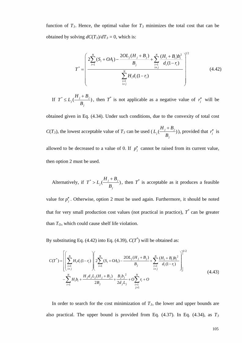
function of T3. Hence, the optimal value for T3 minimizes the total cost that can be
obtained by solving dC(T3)/dT3 = 0, which is:
1 22
1 1*
1
2 ( ) ( )2 ( )(1 )
(1 )
N Nj j j i i i
i ii ij i i
i jN
i i iii j
OL H B H B bS OAB d r
TH d r
= =≠
=≠
+ ++ − + −
= −
∑ ∑
∑ (4.42)
If * ( )j jj
j
H BT L
B+
≤ , then T* is not applicable as a negative value of jr′′ will be
obtained given in Eq. (4.34). Under such conditions, due to the convexity of total cost
C(T3), the lowest acceptable value of T3 can be used ( ( )j jj
j
H BL
B+
), provided that jr′′ is
allowed to be decreased to a value of 0. If jp′′ cannot be raised from its current value,
then option 2 must be used.
Alternatively, if * ( )j jj
j
H BT L
B+
> , then T* is acceptable as it produces a feasible
value for jp′′ . Otherwise, option 2 must be used again. Furthermore, it should be noted
that for very small production cost values (not practical in practice), T* can be greater
than TO, which could cause shelf life violation.
By substituting Eq. (4.42) into Eq. (4.39), C(T*) will be obtained as:
1/2
2*
1 1 1
2
1 11
2 ( ) ( )( ) (1 ) 2 ( )
(1 )
( )2 2
N N Nj j j i i i
i i i i ij i ii i i
i j i j
N Nj j j j j j j
i i ij j ji i
j
OL H B H B bC T H d r S OA
B d r
H d L H B B bH b O r O
B d L
= = =≠ ≠
= =≠
+ +
= − + − + −
+− + + + +
∑ ∑ ∑
∑ ∑
(4.43)
In order to search for the cost minimization of T3, the lower and upper bounds are
also practical. The upper bound is provided from Eq. (4.37). In Eq. (4.34), as T3
105
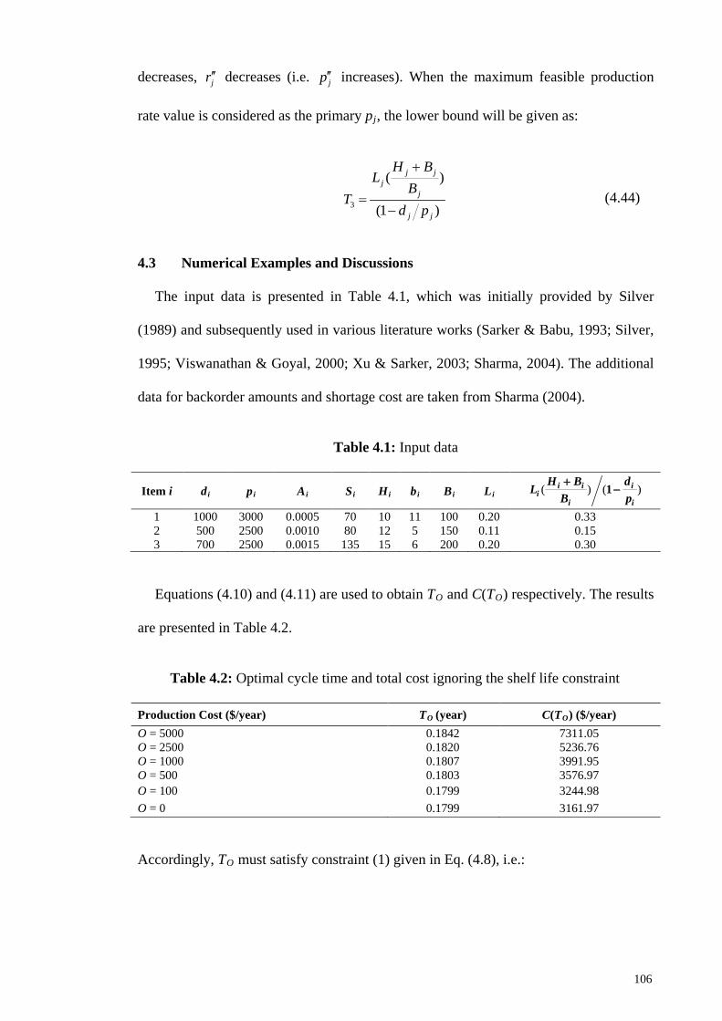
decreases, jr′′ decreases (i.e. jp′′ increases). When the maximum feasible production
rate value is considered as the primary pj, the lower bound will be given as:
3
( )
(1 )
j jj
j
j j
H BL
BT
d p
+
=−
(4.44)
4.3 Numerical Examples and Discussions
The input data is presented in Table 4.1, which was initially provided by Silver
(1989) and subsequently used in various literature works (Sarker & Babu, 1993; Silver,
1995; Viswanathan & Goyal, 2000; Xu & Sarker, 2003; Sharma, 2004). The additional
data for backorder amounts and shortage cost are taken from Sharma (2004).
Table 4.1: Input data
Equations (4.10) and (4.11) are used to obtain TO and C(TO) respectively. The results
are presented in Table 4.2.
Table 4.2: Optimal cycle time and total cost ignoring the shelf life constraint
Production Cost ($/year) TO (year) C(TO) ($/year) O = 5000 0.1842 7311.05 O = 2500 0.1820 5236.76 O = 1000 0.1807 3991.95 O = 500 0.1803 3576.97 O = 100 0.1799 3244.98 O = 0 0.1799 3161.97
Accordingly, TO must satisfy constraint (1) given in Eq. (4.8), i.e.:
Item i di pi Ai Si Hi bi Bi Li ( ) ( )1i i ii
i i
H B dL
B p+
−
1 1000 3000 0.0005 70 10 11 100 0.20 0.33 2 500 2500 0.0010 80 12 5 150 0.11 0.15 3 700 2500 0.0015 135 15 6 200 0.20 0.30
106
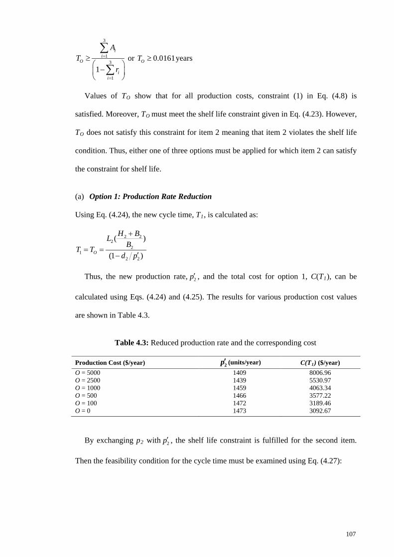
3
13
11
ii
O
ii
AT
r
=
=
≥
−
∑
∑ or 0.0161OT ≥ years
Values of TO show that for all production costs, constraint (1) in Eq. (4.8) is
satisfied. Moreover, TO must meet the shelf life constraint given in Eq. (4.23). However,
TO does not satisfy this constraint for item 2 meaning that item 2 violates the shelf life
condition. Thus, either one of three options must be applied for which item 2 can satisfy
the constraint for shelf life.
(a) Option 1: Production Rate Reduction
Using Eq. (4.24), the new cycle time, T1, is calculated as:
2 22
21
2 2
( )
(1 )O
H BLBT T
d p
+
= =′−
Thus, the new production rate, 2p′ , and the total cost for option 1, C(T1), can be
calculated using Eqs. (4.24) and (4.25). The results for various production cost values
are shown in Table 4.3.
Table 4.3: Reduced production rate and the corresponding cost
Production Cost ($/year) ′2p (units/year) C(T1) ($/year) O = 5000 1409 8006.96 O = 2500 1439 5530.97 O = 1000 1459 4063.34 O = 500 1466 3577.22 O = 100 1472 3189.46 O = 0 1473 3092.67
By exchanging p2 with 2p′ , the shelf life constraint is fulfilled for the second item.
Then the feasibility condition for the cycle time must be examined using Eq. (4.27):
107

32 2
212
3
1
( ) ii
O
iii j
H BL AB
Tr
=
=≠
+−
≤∑
∑ or 0.1888OT ≤ years
Option 1 is feasible as the optimum cycle time TO for all production costs mentioned
in Table 4.2 satisfies this constraint.
(b) Option 2: Cycle Time Reduction
From Eq. (4.28), the adjusted cycle time T2 is obtained as follows:
2 22
22
2 2
( )
(1 )
H BLBT
d p
+
=−
In option 2, the total cost C(T2) can be obtained using Eq. (4.30). The results for
different production costs are shown in Table 4.4.
Table 4.4: Reduced cycle time and the corresponding cost
Production Cost ($/year) T2 (year) C(T2) ($/year) O = 5000 0.1485 7392.62 O = 2500 0.1485 5308.78 O = 1000 0.1485 4058.48 O = 500 0.1485 3641.71 O = 100 0.1485 3308.30 O = 0 0.1485 3224.94
This option is applicable as T2 satisfies the capacity constraint as follows:
3
12 3
11
ii
ii
AT
r
=
=
≥−
∑
∑or 2 0.0161T ≥ years
The comparisons of total cost values obtained from two options are indicated in
Table 4.5. Figure 4.5 represents the trend of cost function values found by two options
for various production cost amounts.
108
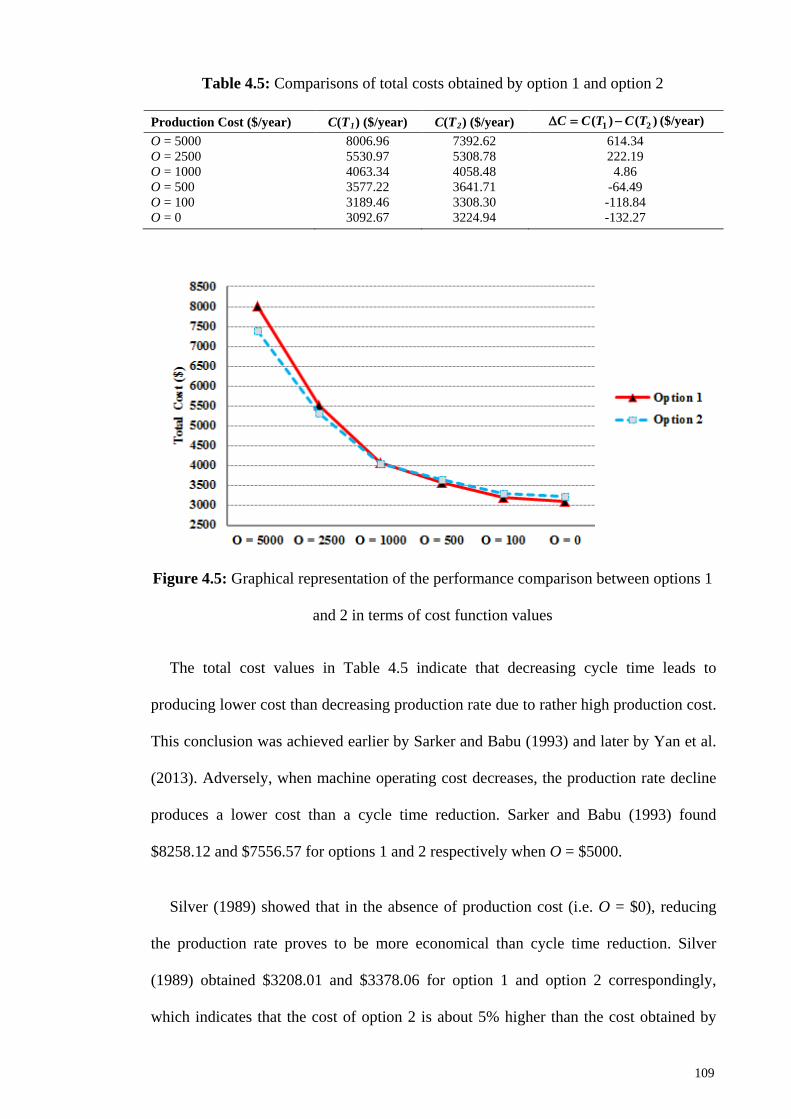
Table 4.5: Comparisons of total costs obtained by option 1 and option 2
Production Cost ($/year) C(T1) ($/year) C(T2) ($/year) 1 2( ) ( )C C T C T∆ = − ($/year) O = 5000 8006.96 7392.62 614.34 O = 2500 5530.97 5308.78 222.19 O = 1000 4063.34 4058.48 4.86 O = 500 3577.22 3641.71 -64.49 O = 100 3189.46 3308.30 -118.84 O = 0 3092.67 3224.94 -132.27
Figure 4.5: Graphical representation of the performance comparison between options 1
and 2 in terms of cost function values
The total cost values in Table 4.5 indicate that decreasing cycle time leads to
producing lower cost than decreasing production rate due to rather high production cost.
This conclusion was achieved earlier by Sarker and Babu (1993) and later by Yan et al.
(2013). Adversely, when machine operating cost decreases, the production rate decline
produces a lower cost than a cycle time reduction. Sarker and Babu (1993) found
$8258.12 and $7556.57 for options 1 and 2 respectively when O = $5000.
Silver (1989) showed that in the absence of production cost (i.e. O = $0), reducing
the production rate proves to be more economical than cycle time reduction. Silver
(1989) obtained $3208.01 and $3378.06 for option 1 and option 2 correspondingly,
which indicates that the cost of option 2 is about 5% higher than the cost obtained by
109
option 1. The model presented in this study offers lower cost for both options compared
to Silver (1989) (3.60% and 4.53% reductions in cost attained by options 1 and 2
respectively).
Clearly, the production cost has significant influence on determining which option to
be selected. According to Sarker and Babu (1993), the preference toward one of these
two options depends on various parameters such as setup time, setup cost, production
cost, holding cost, shortage cost, and shelf time.
It should be noted that slowing down the production rate decreases inventory levels
consistent with a Just-in-Time manufacturing philosophy, hence lowers the inventory
holding cost. However, production rate reduction causes the production to be carried out
for a longer time. If the production time is raised then all related costs such as labor,
machine operating and probably some other associated costs are augmented. Hence,
production rate increase causes some further costs to the manufacturer (Sarker & Babu,
1993). For this reason, production time cost is taken into account in order to include the
effect of the length of production time.
Sharma (2004) inserted shortages into his model, and for production cost of $5000,
total costs $8232.46 and $7454.20 for options 1 and 2 were obtained respectively. The
present model produced lower costs after adjustments to the shelf life constraint and
corresponding mathematical models.
Models with planned backorders have the total related costs reduced, and the items
are stored in inventory for a shorter period of time leading to a less restrictive shelf life
constraint. Furthermore, in this situation, the average inventory level is lower, resulting
in lower inventory holding costs. Negative inventory known as shortage arises when
demand is higher than the production capacity and available inventory. Unsatisfied
110
demand can be backordered and fulfilled in the next period. In a highly competitive
situation in emerging markets, unsatisfied demand will usually be lost. However, this
lost sale usually happens in retail sales than in manufacturing environment. Hence
anticipation for penalty for not fulfilling demand in time (i.e., shortage) is vital in
competitive developing markets (Xu & Sarker, 2003).
(c) Option 3: Adjustment of Production Rate and Cycle Time Concurrently
For this option, two cases should be taken into account as shown in Table 4.6.
Table 4.6: Feasibility assessment of production rate and cycle time reduction
simultaneously
Production Cost ($/year)
3 3 2
1 1
( )( )
2 (1 )i i i
i ii ii i
i j
H B bS OA
d r= =≠
++ +
−∑ ∑ 2 2
22
( )H B
OLB+
O = 5000 267.34 594.00 O = 2500 259.84 297.00 O = 1000 255.34 118.80 O = 500 253.84 59.40 O = 100 252.64 11.88
Table 4.6 indicates that for O = $5000 and $2500, the inequality below applies:
23 3
2 22
1 1 2
( )( ) ( )2 (1 )
i i ii i
i i i ii j
H B b H BS OA OLd r B= =
≠
+ ++ + <
−∑ ∑
Thus, to obtain the minimum total cost, the smallest possible value of T3 should be
chosen (i.e. the smallest possible 2r′′ ). If 2r′′ can be decreased to a very small value
without imposing extra cost, then 2 23 2
2
( )H BT LB+
= or T3 = 0.1188 years should be used,
which results in C(T3) = $6716.14 and $5119.67 for O = $5000 and $2500 respectively.
In this case, the adjusted production rate 2p′′ is infinite. However, if 2r′′ cannot be
reduced (i.e. the production rate cannot exceed its defined maximum value), then option
2 should be chosen with T2 = 0.1485 years, p2 = 2500 units/year, and C(T2) = $7392.62
and $5308.78 for O = $5000 and $2500 respectively.
111
Similarly, in order to find the optimal T3, the lower and upper bounds are applicable.
The upper bound T3 is given as:
32 2
212
3 3
1
( )
/
ii
i iii j
H BL AB
Td p
=
=≠
+−
≤∑
∑ or 3 0.1888T ≤ years
The lower bound T3 is:
2 22
23
2 2
( )0.1485
(1 )
H BLBT
d p
+
= =−
years
The search becomes appropriate for 30.1485 0.1888T≤ ≤ . A simple procedure may
be conducted by reducing T3 from 0.1888 to 0.1485 in a small step, for which the
optimum T3 will be found. By substituting the input data from Table 1 into Eq. (4.39)
and considering that O = $5000, C(T3) is given as:
3 33
276.34( ) 7113.33 8197.16C T TT
= − + +
In line with the search procedure, T3 = 0.1485 years produces the minimum cost, that
is C(T3) = $7392.62. In this case, 2p′′ = 2500 units/year, for which the results are similar
to the findings obtained by option 2 because:
23 32 2
21 1 2
( )( ) ( )2 (1 )
i i ii i
i i i ii j
H B b H BS OA OLd r B= =
≠
+ ++ + <
−∑ ∑ .
For O = $1000, $500 and $100, 23 3
2 22
1 1 2
( )( ) ( )2 (1 )
i i ii i
i i i ii j
H B b H BS OA OLd r B= =
≠
+ ++ + >
−∑ ∑ ;
thus, using Eqs. (4.42) and (4.43), T* and C(T*) can be calculated, and 2p′′ can be
obtained from Eq. (4.34). The results are shown in Table 4.7.
112
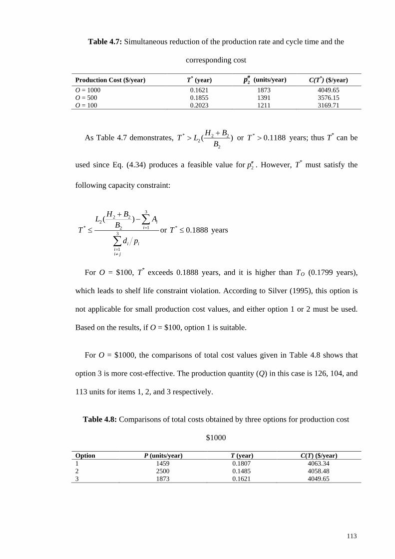
Table 4.7: Simultaneous reduction of the production rate and cycle time and the
corresponding cost
Production Cost ($/year) T* (year) p′′2 (units/year) C(T*) ($/year)
O = 1000 0.1621 1873 4049.65 O = 500 0.1855 1391 3576.15 O = 100 0.2023 1211 3169.71
As Table 4.7 demonstrates, * 2 22
2
( )H BT LB+
> or * 0.1188T > years; thus T* can be
used since Eq. (4.34) produces a feasible value for 2p′′ . However, T* must satisfy the
following capacity constraint:
32 2
2* 12
3
1
( ) ii
i iii j
H BL ABT
d p
=
=≠
+−
≤∑
∑or * 0.1888T ≤ years
For O = $100, T* exceeds 0.1888 years, and it is higher than TO (0.1799 years),
which leads to shelf life constraint violation. According to Silver (1995), this option is
not applicable for small production cost values, and either option 1 or 2 must be used.
Based on the results, if O = $100, option 1 is suitable.
For O = $1000, the comparisons of total cost values given in Table 4.8 shows that
option 3 is more cost-effective. The production quantity (Q) in this case is 126, 104, and
113 units for items 1, 2, and 3 respectively.
Table 4.8: Comparisons of total costs obtained by three options for production cost
$1000
Option P (units/year) T (year) C(T) ($/year) 1 1459 0.1807 4063.34 2 2500 0.1485 4058.48 3 1873 0.1621 4049.65
113
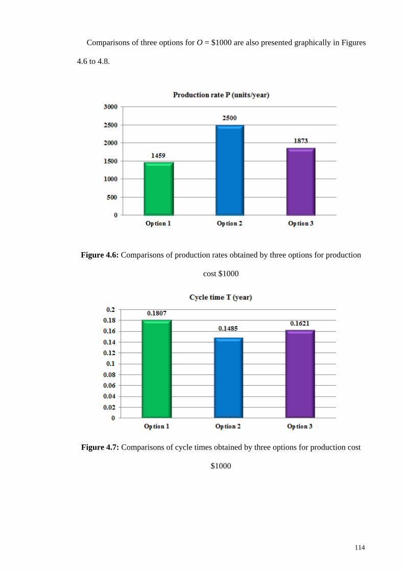
Comparisons of three options for O = $1000 are also presented graphically in Figures
4.6 to 4.8.
Figure 4.6: Comparisons of production rates obtained by three options for production
cost $1000
Figure 4.7: Comparisons of cycle times obtained by three options for production cost
$1000
114
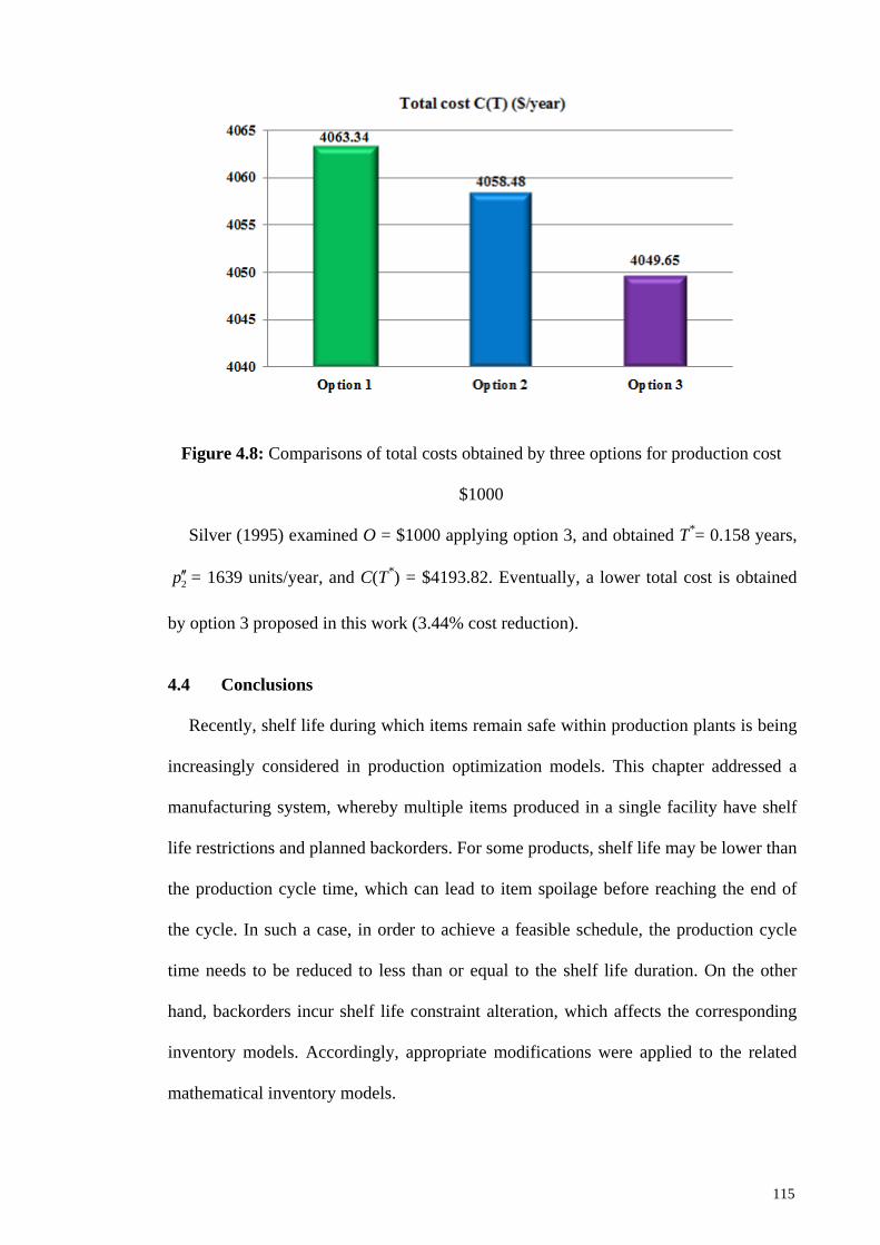
Figure 4.8: Comparisons of total costs obtained by three options for production cost
$1000
Silver (1995) examined O = $1000 applying option 3, and obtained T*= 0.158 years,
2p′′ = 1639 units/year, and C(T*) = $4193.82. Eventually, a lower total cost is obtained
by option 3 proposed in this work (3.44% cost reduction).
4.4 Conclusions
Recently, shelf life during which items remain safe within production plants is being
increasingly considered in production optimization models. This chapter addressed a
manufacturing system, whereby multiple items produced in a single facility have shelf
life restrictions and planned backorders. For some products, shelf life may be lower than
the production cycle time, which can lead to item spoilage before reaching the end of
the cycle. In such a case, in order to achieve a feasible schedule, the production cycle
time needs to be reduced to less than or equal to the shelf life duration. On the other
hand, backorders incur shelf life constraint alteration, which affects the corresponding
inventory models. Accordingly, appropriate modifications were applied to the related
mathematical inventory models.
115
The aim was to determine the optimal cycle time in addition to minimizing the long-
run average costs including production, setup, holding, and shortage costs. While the
cost-minimization cycle time caused the spoilage of products due to shelf life
restrictions, appropriate decisions were made based on one of the three options:
production rate reduction, cycle time reduction, and the simultaneous production rate
and cycle time reduction. As a result, for each option the optimal cycle time and
production rate were estimated, which satisfy the shelf life constraints. Numerical
examples were presented to illustrate the influence of production cost, backorders, and
shelf life on total annual cost.
The superiority of this work stems from the integration of the backorders and shelf
life constraint, and its significant effect on the corresponding inventory models. The
computational results indicated the dominance of the modified models with respect to
producing lower total costs compared to other related models existing in the literature.
116
CHAPTER 5: OPTIMIZATION OF ECONOMIC LOT SCHEDULING
PROBLEM CONSIDERING MULTIPLE SETUPS, BACKORDERING AND
SHELF LIFE USING CALIBRATED METAHEURISTIC ALGORITHMS
5.1 Introduction
This chapter addresses the optimization of the ELSP, where multiple items are
produced on a single machine in a cyclical pattern. It is assumed that each item can be
produced more than once in every cycle, each product has a shelf life restriction, and
backordering is permitted. The objective is to determine the optimal production rate,
production quantity, production frequency, cycle time, as well as a feasible
manufacturing schedule for the family of items, and to minimize the long-run average
costs. Efficient search procedures are presented to obtain the optimum solutions by
employing well-known metaheuristic algorithms.
The rest of this chapter is organized as follows: Section 5.2 presents the proposed
mixed integer non-linear ELSP model. In Section 5.3, metaheuristic algorithms namely
the GA, PSO, ABC, and SA are explained to solve the proposed model. Section 5.4
describes the Taguchi method employed to tune various parameters of the applied
algorithms. Section 5.5 demonstrates the numerical example and discusses the
computational results. Finally, conclusions are given in Section 5.6.
5.2 Problem Description and Mathematical Formulations
The ELSP in this study is considered in a single machine environment with
production of N items in the manufacturing cycle time of T, where backordering is
permitted for any of the items, and each of which has a specified shelf life. Moreover,
the restricted assumption of production of every item exactly once in a cycle considered
in previous studies is removed, and it is allowed to produce each item more than once in
every cycle.
117
The objective is to find the optimal production rate, production frequency, cycle
time, and batch size of each item as well as a feasible manufacturing schedule for the
family of items. Furthermore, it is attempted to minimize the long-run average cost
including setup, production, holding, and backorder costs, in addition to the adjustment
cost if production time conflicts are occurred between the products in a cycle.
The mathematical model studied throughout this chapter is based on the following
assumptions and notations:
(a) Assumptions
i. Each item has a deterministic and constant demand.
ii. Each item has a deterministic and constant setup time.
iii. The first-in-first-out rule is considered for the inventory transactions.
(b) Indices
i Product (i = 1, 2, … , N)
N Total number of products
j Batch number (j = 1, 2, …, fi)
w, w’ Production batch (w, w’ = 1, 2, … , 1
N
ii
F f=
= ∑ )
(c) Parameters
id Demand rate for item i (units/year)
maxiP Maximum possible production rate for item i (units/year)
miniR Ratio of demand to maximum production rate for item i
iL Shelf life of item i (years)
iA Setup time for item i (years)
118
iS Setup cost for item i (dollars/unit/year) (machine operating cost is excluded
during setup)
iH Inventory holding cost for item i (dollars/unit/year)
iB Backordering cost for item i (dollars/unit/year)
O Machine operating cost (dollars/year)
(d) Variables
ip Production rate for item i
ir Ratio of demand to production rate for item i
if Production frequency for item i per cycle
it Cycle time for item i
ik Production start time for item i
iτ Production time for item i
jiα Production start time advancement for item i in its jth production batch
jiβ Production start time delay for item i in its jth production batch
iϑ Machine time for item i
iQ Production batch size of item i
ib Amount of item i backordered in each cycle
im Maximum backorder level for item i
T Entire production cycle time
( )C T Total cost for the entire production cycle time
1 if item is produced in the batch0 otherwise
thwi
i wψ
119
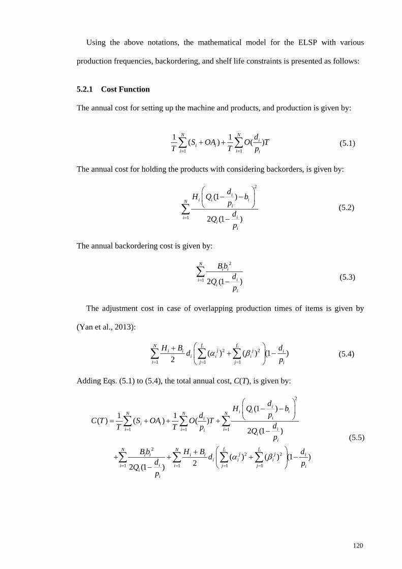
Using the above notations, the mathematical model for the ELSP with various
production frequencies, backordering, and shelf life constraints is presented as follows:
5.2.1 Cost Function
The annual cost for setting up the machine and products, and production is given by:
1 1
1 1( ) ( )N N
ii i
i i i
dS OA O TT T p= =
+ +∑ ∑ (5.1)
The annual cost for holding the products with considering backorders, is given by:
2
1
(1 )
2 (1 )
ii i iN
i
iii
i
dH Q bp
dQp
=
− −
−∑ (5.2)
The annual backordering cost is given by:
2
1 2 (1 )
Ni i
iii
i
B bdQp
= −∑
(5.3)
The adjustment cost in case of overlapping production times of items is given by
(Yan et al., 2013):
2 2
1 1 1( ) ( ) (1 )
2
i if fNj ji i i
i i ii j j i
H B ddp
α β= = =
++ −
∑ ∑ ∑ (5.4)
Adding Eqs. (5.1) to (5.4), the total annual cost, C(T), is given by:
2
1 1 1
22 2
1 1 1 1
(1 )1 1( ) ( ) ( )
2 (1 )
( ) ( ) (1 )22 (1 )
i i
ii i iN N N
iii i
ii i iii
i
f fN Nj ji i i i i
i i iii i j j i
ii
dH Q bpdC T S OA O T dT T p Q
p
B b H B ddd pQp
α β
= = =
= = = =
− −
= + + +−
++ + + −
−
∑ ∑ ∑
∑ ∑ ∑ ∑
(5.5)
120
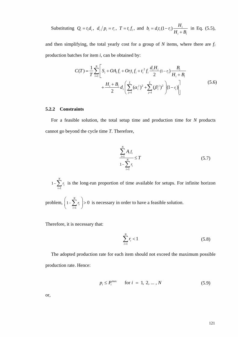
Substituting i i iQ t d= , i i id p r= , i iT t f= , and (1 ) ii i i i
i i
Hb d t rH B
= −+
in Eq. (5.5),
and then simplifying, the total yearly cost for a group of N items, where there are fi
production batches for item i, can be obtained by:
2
1
2 2
1 1
(11( ) )
2
( ) ( ) (1 )2
i i
Ni i i
i i i i i i i i ii i i
f fj ji i
i i i ij j
r
r
d H BC T S OA f Ort f t fT H B
H B d
=
= =
−
= + + + + +
+ + −
∑
∑ ∑α β (5.6)
5.2.2 Constraints
For a feasible solution, the total setup time and production time for N products
cannot go beyond the cycle time T. Therefore,
1
11
N
i ii
N
ii
f
r
AT=
=
−
≤∑
∑ (5.7)
11
=
− ∑N
ii
r is the long-run proportion of time available for setups. For infinite horizon
problem, 1
1 0=
−
>
∑N
ii
r is necessary in order to have a feasible solution.
Therefore, it is necessary that:
1
1N
ii
r=
<∑ (5.8)
The adopted production rate for each item should not exceed the maximum possible
production rate. Hence:
max for 1, 2, ... , i ip P i N≤ = (5.9)
or,
121
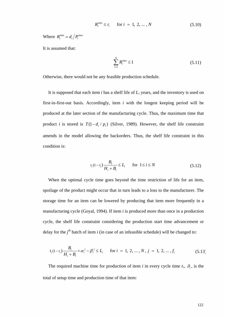
min for 1, 2, ... , i iR r i N≤ = (5.10)
Where min maxi i iR d P=
It is assumed that:
min
11
N
ii
R=
≤∑ (5.11)
Otherwise, there would not be any feasible production schedule.
It is supposed that each item i has a shelf life of Li years, and the inventory is used on
first-in-first-out basis. Accordingly, item i with the longest keeping period will be
produced at the later section of the manufacturing cycle. Thus, the maximum time that
product i is stored is (1 / )i iT d p− (Silver, 1989). However, the shelf life constraint
amends in the model allowing the backorders. Thus, the shelf life constraint in this
condition is:
(1 ) for 1ii i i
i i
t rB L i N
H B− ≤ ≤ ≤
+ (5.12)
When the optimal cycle time goes beyond the time restriction of life for an item,
spoilage of the product might occur that in turn leads to a loss to the manufacturer. The
storage time for an item can be lowered by producing that item more frequently in a
manufacturing cycle (Goyal, 1994). If item i is produced more than once in a production
cycle, the shelf life constraint considering the production start time advancement or
delay for the jth batch of item i (in case of an infeasible schedule) will be changed to:
(1 ) for 1, 2, ... , , 1, 2, ... , j jii i i i i i
i i
rBt L i N j f
H Bα β− + − ≤ = =
+ (5.13)
The required machine time for production of item i in every cycle time ti, iϑ , is the
total of setup time and production time of that item:
122
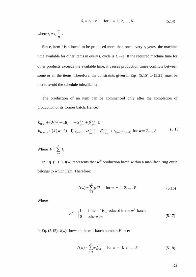
for 1, 2, ... , i i iA i Nϑ τ= + = (5.14)
where ii i
i
dtp
τ = .
Since, item i is allowed to be produced more than once every ti years, the machine
time available for other items in every ti cycle is iit ϑ− . If the required machine time for
other products exceeds the available time, it causes production times conflicts between
some or all the items. Therefore, the constraints given in Eqs. (5.15) to (5.21) must be
met to avoid the schedule infeasibility.
The production of an item can be commenced only after the completion of
production of its former batch. Hence:
1 1
1 11 1 1 1
( 1)
( 1 1) for 2,...,
J w J w
I w I w
J w J w
I w I w
I w I w
I w I w I w I wr t
k J w t
k J w t w F
( ) ( )
( ) ( )
( − ) ( − )
( − ) ( − )
( ) ( )
( − ) ( − ) ( − ) ( − )
+ ( ) − − + ≥
+ ( − ) − − + + =
α β
α β
(5.15)
Where 1
N
ii
F f=
= ∑
In Eq. (5.15), I(w) represents that wth production batch within a manufacturing cycle
belongs to which item. Therefore:
1
( ) for 1, 2, ... , N
wi
iI w i w Fψ
=
= =∑ (5.16)
Where
1 if item is produced in the batch0 otherwise
thwi
i w=
ψ (5.17)
In Eq. (5.15), J(w) shows the item’s batch number. Hence:
( )1
( ) for 1, 2, ... , w
wI w
wJ w w Fψ ′
′=
= =∑ (5.18)
123
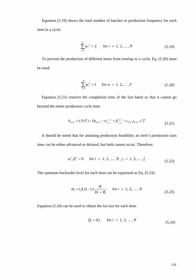
Equation (5.19) shows the total number of batches or production frequency for each
item in a cycle:
1
for 1, 2, ... , F
wi i
wf i Nψ
=
= =∑ (5.19)
To prevent the production of different items from overlap in a cycle, Eq. (5.20) must
be used:
1
1 for 1, 2, ... , N
wi
iw Fψ
=
= =∑ (5.20)
Equation (5.21) restricts the completion time of the last batch so that it cannot go
beyond the entire production cycle time:
( 1) J F J F
I F I FI F I F I F I Fr tk J F t Tα β( ) ( )
( ) ( )( ) ( ) ( ) ( )+ ( ) − − + + ≤ (5.21)
It should be noted that for attaining production feasibility an item’s production start
time can be either advanced or delayed, but both cannot occur. Therefore:
. 0 for 1, 2, ... , , 1, 2, ... , j ji i ii N j fα β = = = (5.22)
The optimum backorder level for each item can be expressed as Eq. (5.23):
(1 ) for 1, 2, ... , i
i i i ii i
Hm t d r i NH B
= − =+
(5.23)
Equation (5.24) can be used to obtain the lot size for each item:
for 1, 2, ... , i i iQ d t i N= = (5.24)
124
Constraints (5.25) are the non-negativity constraints:
00 for 1, 2, ... ,
, 0 for 1, 2, ... , , 1, 2, ... , 0 integer for 1, 2, ... ,
ij j
i i i
i
Tr i N
i N j ff i N
α β
≥≥ =
≥ = =
> =
(5.25)
5.3 Solution Algorithms
The formulation given in Section 5.2 is a nonlinear mixed integer problem. These
characteristics justify the model to be adequately difficult to solve using the exact
methods. To deal with the intricacy and obtain near-optimal results in a reasonable
computation time, metaheuristic approaches are widely used for which the GA, PSO,
ABC, and SA methods are explained in the following subsections. Related codes are
presented in Appendices A to D.
5.3.1 GA Approach
The GA is a type of stochastic optimization method that randomly searches the
solution space to find a solution (Parsapoor & Bilstrup, 2012). The general steps of the
GA can be summarized as follow (Gen & Cheng, 2008):
i. Encoding solutions of problem into chromosomes.
ii. Creating initial population of solutions randomly.
iii. Evaluating chromosomes in terms of their fitness in order to select parents.
iv. Applying genetic operators (crossover and mutation) in order to reproduce new
chromosomes (offspring).
v. Evaluating the new population.
vi. Maintain the best chromosomes among parents and offspring.
vii. If stopping criteria is met, then stop. Otherwise, go to step iii.
125
The required steps to solve the proposed model by a GA are explained below.
(a) Initial Conditions
The initial information required to begin a GA includes:
1. The number of chromosomes kept in each generation that is named population
size, and indicated by ‘Npop’.
2. The probability of operating crossover known as crossover rate represented by
‘Pc’.
3. The probability of operating mutation called mutation rate represented by ‘Pm’.
4. Maximum number of iterations denoted by ‘max iter’.
Both the crossover and mutation rates alter in the range [0.1, 1]. The computational
results show that the effect of Pc on the total cost value is positive. Therefore, the
smaller the crossover probability, the lesser the total cost will be. However, C(T)
decreases as Pm increases.
Npop, Pc, and Pm are calibrated using the Taguchi method descried in Section 5.4.
(b) Chromosome Representation
One of the most important factors for effective application of the GA is creating an
appropriate chromosomal structure. A GA starts with encoding the variables of the
problem as finite-length strings. These strings are called chromosomes. The number of
genes in a chromosome is equal to decision variables. As proposed model in this study
is a non-linear problem containing three different types of variables (discrete,
continuous, and binary), a real number representation is applied to reduce this
complexity. Matrices X1, X2, and X3 present the general form of chromosomes:
126
1 21
1 2
... ...
=
N
N
p p pX
t t t (5.26)
Matrix X1 contains two rows and N columns. The two elements of each column
represent the adopted production rate p (integer) and cycle time t (floating point) for
each item respectively.
1 21 1 11 22 2 2
1
2
2
...
... . . . . . . . . . . . .
...
=
F
F
FN N N
X
ψ ψ ψ
ψ ψ ψ
ψ ψ ψ
(5.27)
X2 is a N F× matrix of binary values for the variable wiψ . N shows the total number
of products, and F indicates the total number of production frequencies for all items. To
have a feasible schedule for each column only one non-zero value of 1 must be
generated, and the rest of elements are 0. The mechanism of generating 1 and 0 is
random (1 and 0 indicate that the item is produced or not during cycle time T).
Summation of values in each row shows the production frequency for each item.
When the GA generates a random initial population for variable ψ , the matrix may
have more than one value of 1 in each column. Therefore, the columns of matrix ψ
must be rechecked. If the number of value of 1 in per column is greater than one, the
values of 1 must be changed to 0, and only one value of 1 should be kept. In order to
decide which of those 1s must be converted to 0, a cost for each element is considered
in the form of ( )/i iO d p× . The 1s with higher costs will be changed to 0, and only one
element with the lowest cost is kept.
127
1 1 2 21 1 1 1 1 11 1 2 22 2 2 2 2 2
3
, , ... ,
, , ... , . . . . . . . . . . .
=
F F
F F
X
α β α β α β
α β α β α β
1 1 2 2
., , ... ,
F FN N N N N Nα β α β α β
(5.28)
As products are allowed to have more than one setup per cycle, it might cause an
infeasible production plan. In order to attain feasibility, the production start time of
some items can be advanced ( jiα ) or delayed ( j
iβ ). However, the start time for a
product can be adjusted by either advancing or delaying, but not both. Matrix X3,
containing N rows and F columns, represents the chromosome for the floating point
variables jiα and j
iβ .
(c) Initial Population
The GA generates a randomly initial population of g chromosomes, where g denotes
the size of population. Let Xg = Xg1, Xg2, . . . , Xgd indicates the gth chromosome in the
population, and each solution Xg is a D-dimensional vector, where D refers to the
optimization variables. Then, the GA updates boundaries for each variable using Eq.
(5.29):
( ) for 1, 2, ..., and 1, 2, ... , gn n n n popX lb y ub lb g N n D= + × − = = (5.29)
Where y is a random number in the range [0, 1], and lbn and ubn are the lower and
upper bounds for the dimension n, respectively. For the integer variables, Xgn is
rounded.
(d) Evaluation and Constraint Handling
When chromosomes are produced, a fitness value must be assigned to chromosomes
of each generation in order to evaluate them. This evaluation is achieved by the
128
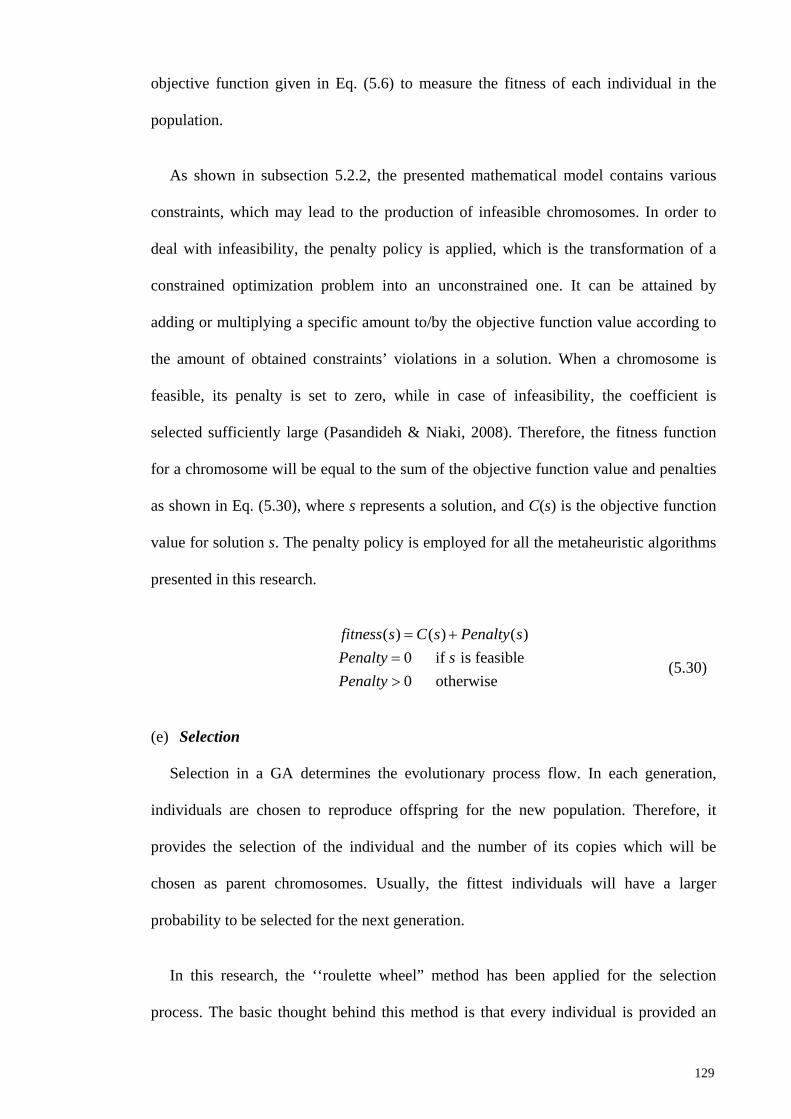
objective function given in Eq. (5.6) to measure the fitness of each individual in the
population.
As shown in subsection 5.2.2, the presented mathematical model contains various
constraints, which may lead to the production of infeasible chromosomes. In order to
deal with infeasibility, the penalty policy is applied, which is the transformation of a
constrained optimization problem into an unconstrained one. It can be attained by
adding or multiplying a specific amount to/by the objective function value according to
the amount of obtained constraints’ violations in a solution. When a chromosome is
feasible, its penalty is set to zero, while in case of infeasibility, the coefficient is
selected sufficiently large (Pasandideh & Niaki, 2008). Therefore, the fitness function
for a chromosome will be equal to the sum of the objective function value and penalties
as shown in Eq. (5.30), where s represents a solution, and C(s) is the objective function
value for solution s. The penalty policy is employed for all the metaheuristic algorithms
presented in this research.
( ) ( ) ( )0 if is feasible0 otherwise
= +=>
fitness s C s Penalty sPenalty sPenalty
(5.30)
(e) Selection
Selection in a GA determines the evolutionary process flow. In each generation,
individuals are chosen to reproduce offspring for the new population. Therefore, it
provides the selection of the individual and the number of its copies which will be
chosen as parent chromosomes. Usually, the fittest individuals will have a larger
probability to be selected for the next generation.
In this research, the ‘‘roulette wheel” method has been applied for the selection
process. The basic thought behind this method is that every individual is provided an
129
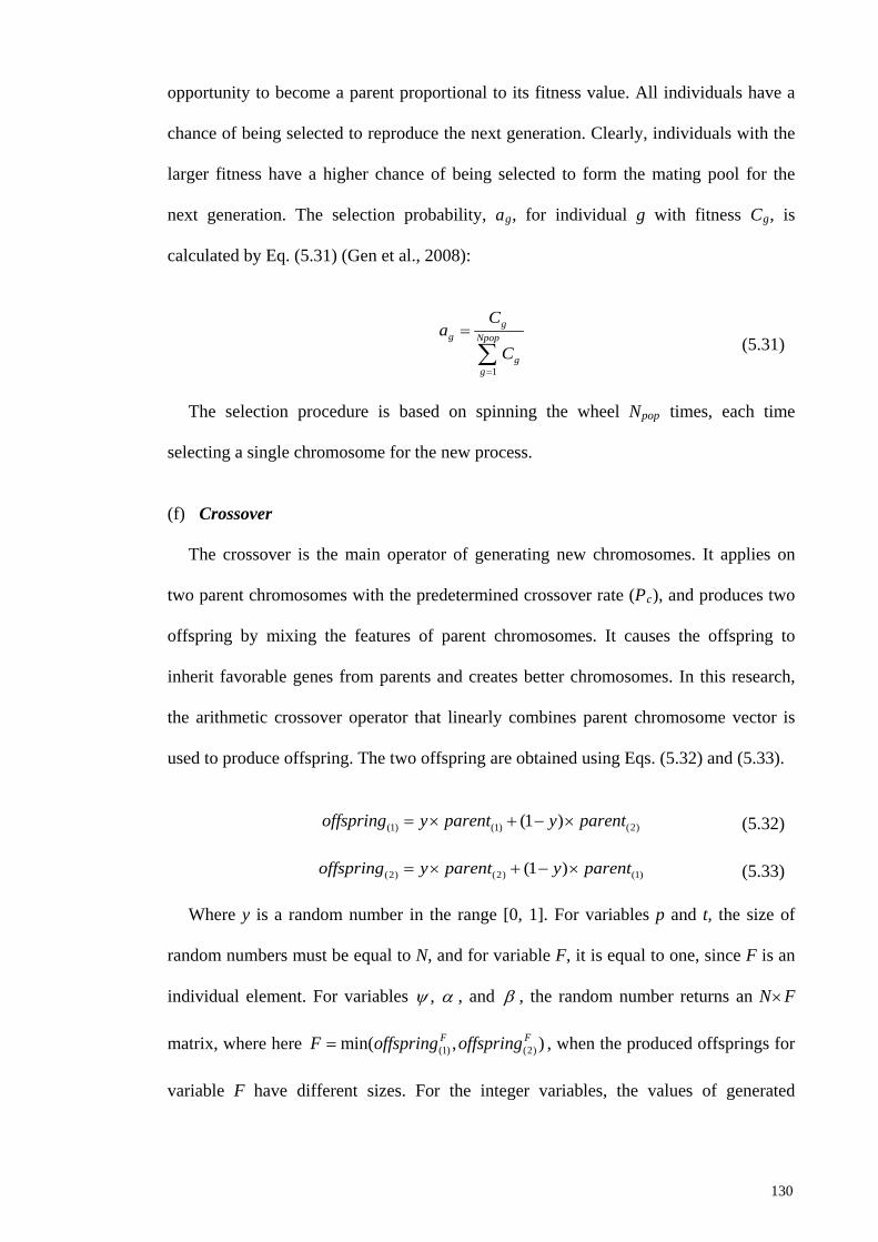
opportunity to become a parent proportional to its fitness value. All individuals have a
chance of being selected to reproduce the next generation. Clearly, individuals with the
larger fitness have a higher chance of being selected to form the mating pool for the
next generation. The selection probability, ag, for individual g with fitness Cg, is
calculated by Eq. (5.31) (Gen et al., 2008):
1
gg Npop
gg
Ca
C=
=
∑
(5.31)
The selection procedure is based on spinning the wheel Npop times, each time
selecting a single chromosome for the new process.
(f) Crossover
The crossover is the main operator of generating new chromosomes. It applies on
two parent chromosomes with the predetermined crossover rate (Pc), and produces two
offspring by mixing the features of parent chromosomes. It causes the offspring to
inherit favorable genes from parents and creates better chromosomes. In this research,
the arithmetic crossover operator that linearly combines parent chromosome vector is
used to produce offspring. The two offspring are obtained using Eqs. (5.32) and (5.33).
(1) (1) (2)(1 )offspring y parent y parent= × + − × (5.32)
(2) (2) (1)(1 )offspring y parent y parent= × + − × (5.33)
Where y is a random number in the range [0, 1]. For variables p and t, the size of
random numbers must be equal to N, and for variable F, it is equal to one, since F is an
individual element. For variables , ψ α , and β , the random number returns an N×F
matrix, where here (1) (2)min( , )= F FF offspring offspring , when the produced offsprings for
variable F have different sizes. For the integer variables, the values of generated
130
offsprings by Eqs. (5.32) and (5.33) are rounded to the nearest integer amount. Figure
5.1 shows how the crossover operator for the continuous variables , , and j ji i it α β works.
Figure 5.1: An example of a crossover operation
(g) Mutation
Mutation exerts stochastic change in chromosome genes with probability Pm. It is
considered as a background operator that keeps genetic diversity within the population.
Mutation may contribute in preventing the algorithm to get stuck at a local minimum as
well as reaching an untimely convergence. It ensures that the irreversible loss of genetic
information does not take place. First, a random number in range [0, 1] is generated.
Then, if random number is less than 0.5, Eq. (5.33), and if it is greater than 0.5, Eq.
(5.34) will be used to mutate the selected genes. Suppose a particular gene such as Xk is
chosen for mutation; then the value of Xk will be changed to the new value X’k using
Eqs. (5.34) and (5.35):
1 (X )max iter
′ = − × − × −
k k k kX X y lbρ (5.34)
1 ( )max iter
′ = + × − × −
k k k kX X y ub Xρ (5.35)
y = 0.9
131
Where k is an integer value in range [1, N], lbk and ubk are the lower and upper
bounds of the specific gene, y is a random variable in the range [0, 1], and ρ is the
number of current iteration. For the integer variables, the values obtained by Eqs. (5.34)
and (5.35) are rounded.
For the binary variable ψ , an integer number in the range [1, (N×F)] is generated in
order to select the element of matrix ψ . Then, if the chosen element is 1, it will be
replaced with 0, and vice versa. For variables α and β , first, an integer number in the
range [1, (N×F)] is produced to select the element. Then, a random number in the range
[0, 1] is generated. If it is less than 0.5, Eq. (5.36), and if it is greater than 0.5, Eq. (5.37)
will be used to mutate the selected element.
1 ( 0)max iter
′ = − × − × −
k k kX X y Xρ (5.36)
1 (1 )max iter
′ = + × − × −
k k kX X y Xρ (5.37)
(h) New Population
Fitness function value of all members, including parents and offspring are assessed in
this stage. Next, the chromosomes with higher fitness scores are selected to create a new
population. To attain a better solution, the fittest chromosomes must be maintained at
the end of this stage. Note that the number of selected chromosomes must be equal to
Npop.
(i) Termination
The selection and reproduction of parents will be continued until the algorithm
reaches a stopping criterion. The procedure can be ended after a predetermined number
of iterations, or when no substantial improvement during any iteration is achieved. In
this study, the procedure terminates when the algorithm reaches the maximum number
132
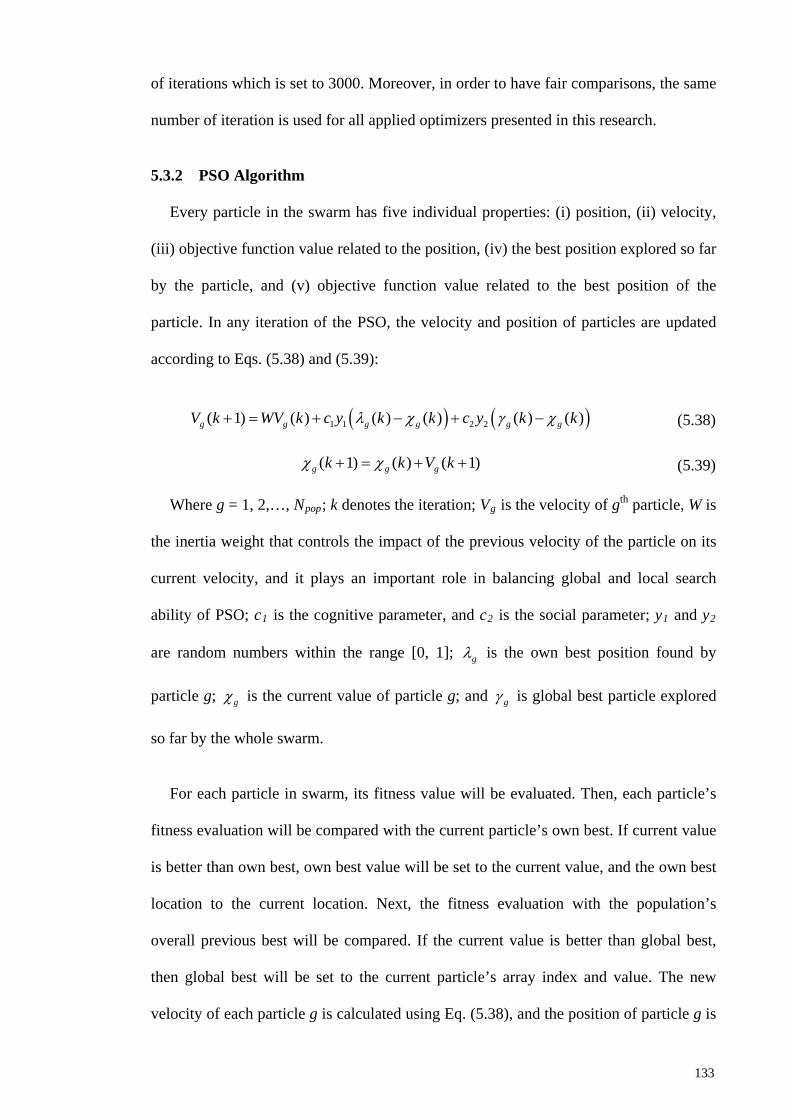
of iterations which is set to 3000. Moreover, in order to have fair comparisons, the same
number of iteration is used for all applied optimizers presented in this research.
5.3.2 PSO Algorithm
Every particle in the swarm has five individual properties: (i) position, (ii) velocity,
(iii) objective function value related to the position, (iv) the best position explored so far
by the particle, and (v) objective function value related to the best position of the
particle. In any iteration of the PSO, the velocity and position of particles are updated
according to Eqs. (5.38) and (5.39):
( ) ( )1 1 2 2( 1) ( ) ( ) ( ) ( ) ( )+ = + − + −g g g g g gV k WV k c y k k c y k kλ χ γ χ (5.38)
( 1) ( ) ( 1)+ = + +g g gk k V kχ χ (5.39)
Where g = 1, 2,…, Npop; k denotes the iteration; Vg is the velocity of gth particle, W is
the inertia weight that controls the impact of the previous velocity of the particle on its
current velocity, and it plays an important role in balancing global and local search
ability of PSO; c1 is the cognitive parameter, and c2 is the social parameter; y1 and y2
are random numbers within the range [0, 1]; gλ is the own best position found by
particle g; gχ is the current value of particle g; and gγ is global best particle explored
so far by the whole swarm.
For each particle in swarm, its fitness value will be evaluated. Then, each particle’s
fitness evaluation will be compared with the current particle’s own best. If current value
is better than own best, own best value will be set to the current value, and the own best
location to the current location. Next, the fitness evaluation with the population’s
overall previous best will be compared. If the current value is better than global best,
then global best will be set to the current particle’s array index and value. The new
velocity of each particle g is calculated using Eq. (5.38), and the position of particle g is
133
updated by Eq. (5.39), which is adding its new velocity to its current position. This
process continues until stopping condition is satisfied, which is reaching the maximum
number of iterations equal to 3000.
5.3.3 ABC Algorithm
The ABC algorithm was inspired by the honey bee foraging behavior. The ABC
method includes four main components, namely food sources, employed bees, onlooker
bees, and scout bees. The main steps of the ABC procedure are described below.
(a) Initialization of the Parameters
The main parameters of the ABC algorithm are the colony size (NB), number of food
sources (NS), number of trials after which a food source is supposed to be discarded
(limit), and maximum number of cycles of the search process (MCN). Several
combinations of NB and limit have been implemented by applying Taguchi method
described in Section 5.4 The number of food sources (NS) is considered as NB/2. MCN
is set to 3000.
The first half of the colony consists of the employed artificial bees and the second
half includes the onlookers. For every food source, there is only one employed bee, i.e.
the number of employed bees is equal to the number of food sources around the hive
(Karaboga, 2005).
(b) Initialization of the Population
The ABC algorithm generates a randomly initial population of g solutions (g = 1, 2,
... , NS). Then the algorithm updates boundaries for each variable using Eq. (5.29). After
initialization, the population of the food source positions is commanded to iterate the
cycle of search processes for the employed, onlooker and scout bees (cycle = 1, 2, . . . ,
MCN).
134
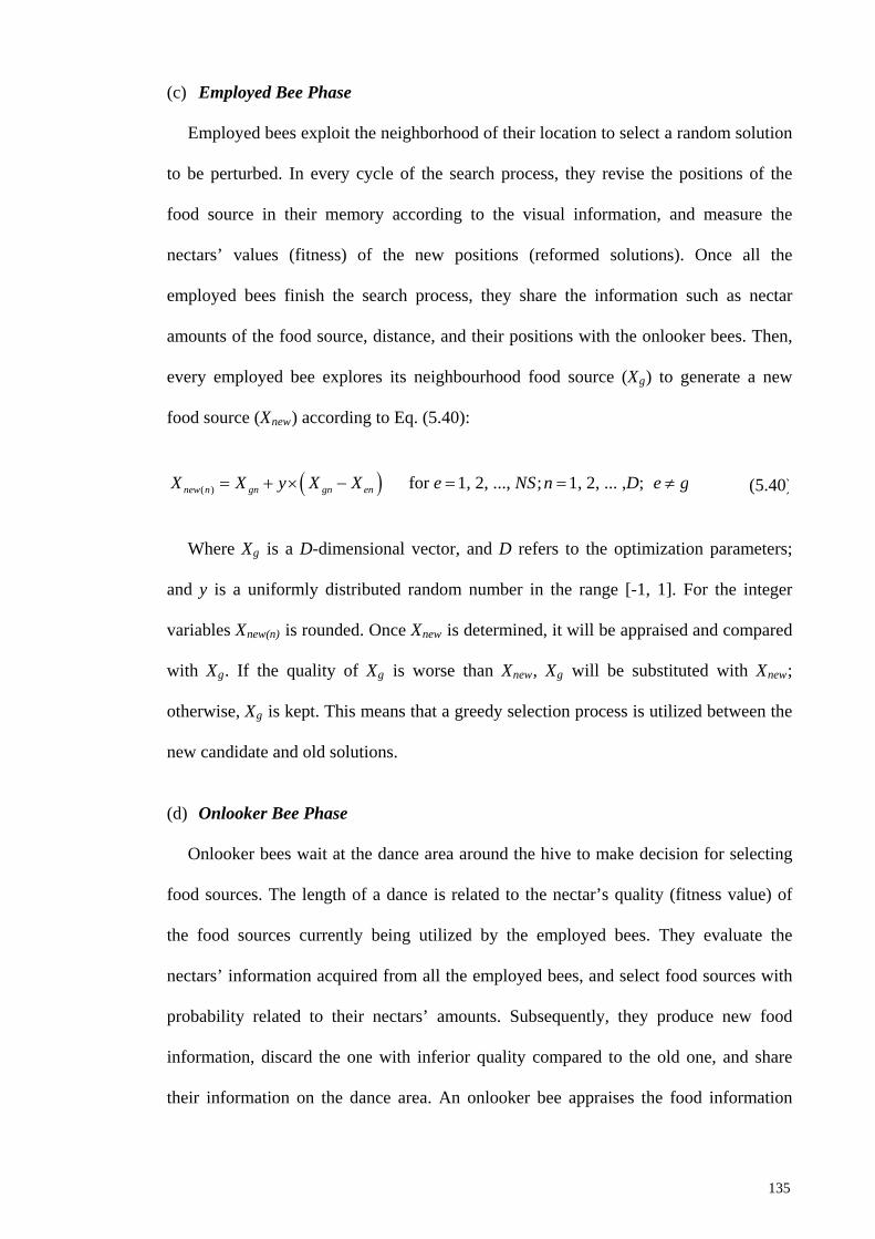
(c) Employed Bee Phase
Employed bees exploit the neighborhood of their location to select a random solution
to be perturbed. In every cycle of the search process, they revise the positions of the
food source in their memory according to the visual information, and measure the
nectars’ values (fitness) of the new positions (reformed solutions). Once all the
employed bees finish the search process, they share the information such as nectar
amounts of the food source, distance, and their positions with the onlooker bees. Then,
every employed bee explores its neighbourhood food source (Xg) to generate a new
food source (Xnew) according to Eq. (5.40):
( )( ) for 1, 2, ..., ; 1, 2, ... , ; new n gn gn enX X y X X e NS n D e g= + × − = = ≠
(5.40)
Where Xg is a D-dimensional vector, and D refers to the optimization parameters;
and y is a uniformly distributed random number in the range [-1, 1]. For the integer
variables Xnew(n) is rounded. Once Xnew is determined, it will be appraised and compared
with Xg. If the quality of Xg is worse than Xnew, Xg will be substituted with Xnew;
otherwise, Xg is kept. This means that a greedy selection process is utilized between the
new candidate and old solutions.
(d) Onlooker Bee Phase
Onlooker bees wait at the dance area around the hive to make decision for selecting
food sources. The length of a dance is related to the nectar’s quality (fitness value) of
the food sources currently being utilized by the employed bees. They evaluate the
nectars’ information acquired from all the employed bees, and select food sources with
probability related to their nectars’ amounts. Subsequently, they produce new food
information, discard the one with inferior quality compared to the old one, and share
their information on the dance area. An onlooker bee appraises the food information
135
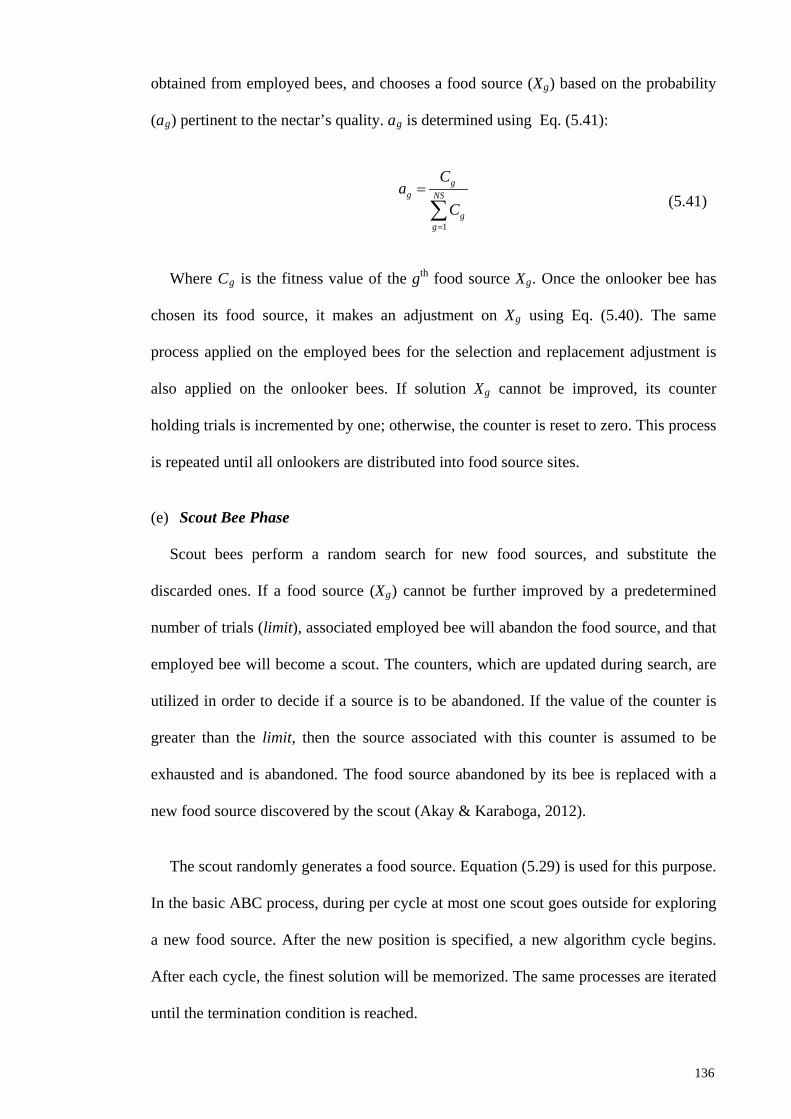
obtained from employed bees, and chooses a food source (Xg) based on the probability
(ag) pertinent to the nectar’s quality. ag is determined using Eq. (5.41):
1
gg NS
gg
Ca
C=
=
∑
(5.41)
Where Cg is the fitness value of the gth food source Xg. Once the onlooker bee has
chosen its food source, it makes an adjustment on Xg using Eq. (5.40). The same
process applied on the employed bees for the selection and replacement adjustment is
also applied on the onlooker bees. If solution Xg cannot be improved, its counter
holding trials is incremented by one; otherwise, the counter is reset to zero. This process
is repeated until all onlookers are distributed into food source sites.
(e) Scout Bee Phase
Scout bees perform a random search for new food sources, and substitute the
discarded ones. If a food source (Xg) cannot be further improved by a predetermined
number of trials (limit), associated employed bee will abandon the food source, and that
employed bee will become a scout. The counters, which are updated during search, are
utilized in order to decide if a source is to be abandoned. If the value of the counter is
greater than the limit, then the source associated with this counter is assumed to be
exhausted and is abandoned. The food source abandoned by its bee is replaced with a
new food source discovered by the scout (Akay & Karaboga, 2012).
The scout randomly generates a food source. Equation (5.29) is used for this purpose.
In the basic ABC process, during per cycle at most one scout goes outside for exploring
a new food source. After the new position is specified, a new algorithm cycle begins.
After each cycle, the finest solution will be memorized. The same processes are iterated
until the termination condition is reached.
136
5.3.4 SA Algorithm
The SA algorithm is a local search method inspired by the physical annealing process
studied in statistical mechanics and was initially proposed for combinatorial
optimization problems. The SA algorithm repeats an iterative neighbor generation
procedure and follows search directions that aim to improve the objective function value
towards the global optimum. The main steps of the SA algorithm are described below.
(a) Initialization
In this step, the input parameters of the SA algorithm are initialized. The parameters
are:
i. Initial Temperature
The initial temperature (E0) is the starting point of temperature computation in every
iteration. E0 should be adequately high to escape a premature convergence. Basically,
the SA algorithm starts with an initial temperature where almost all worsening moves
are accepted regardless of the objective function value.
ii. Iteration
It shows the number of iteration in each temperature.
iii. Final Temperature
The temperature is remained fixed once it reaches the lowest temperature limit (Ef).
(b) Cooling Schedule
System temperature determines the degree of randomness towards solution, and it is
reduced with a known plan in accordance with the progress of solution procedure. In
reality, system temperature is a solution subspace of the problem accepted in each
iteration. As the algorithm progresses and the temperature decreases, inappropriate
137
solutions have smaller chance of being accepted. Cooling schedule determines the
functional form of the change in temperature required in the SA.
A geometric temperature reduction rule, which is the most commonly utilized
decrement rule, is applied for this study. If the temperature at kth iteration is Ek, then the
temperature at (k+1)th iteration is given by (Kirkpatrick, 1984):
1+ = ×k kE z E (5.42)
Where z denotes the cooling factor in the range [0, 1].
(c) Neighborhood Representation
The neighborhood search structure is a procedure that generates a new solution that
slightly changes the current solution. To delineate the neighborhood configuration, the
following process is used in order to prevent the fast convergence of the SA. The
number of neighborhood searches in each temperature level (epoch length) is
considered to be 10. It is the number of solutions which are accessible in an immediate
move from the current solution.
Suppose a particular vector such as Xk is selected; then the value of Xk will be
changed to the new value X’k using Eqs. (5.43) and (5.44).
0.1 ( )k k k kX X y X lb′ = − × × − (5.43)
0.1 ( )k k k kX X y ub X′ = + × × − (5.44)
Where k is an integer value in range [1, N], lbk and ubk are the lower and upper
bounds of the specific vector, and y is a random variable in the range [0, 1]. For the
integer variables the values obtained by Eqs. (5.43) and (5.44) are rounded.
For the binary variable ψ , two integer numbers y1 and y2 are generated, where y1 is
in range [1, ( N F× ) -1] and y2 is in range [y1+1, N F× ] in order to select the elements
138
of matrix ψ . Then, if the elements in the selected columns are 1s, they will be replaced
with 0s, and vice versa.
For variablesα and β , the same integer numbers y1 and y2 are used to select the
elements. Then the following equations are employed to change the chosen elements:
( )1 2 1 2 1 2( : ) ( : ) ( : )0.1 0y y y y y yX X y X′ = − × × − (5.45)
( )1 2 1 2 1 2( : ) ( : ) ( : )0.1 1y y y y y yX X y X′ = + × × − (5.46)
Where y is a random number in the range [0, 1]. The quantity of generated random
numbers must be equal to 2 1( 1)y y− + .
For selecting which equation to be used, a random number in the range [0, 1] is
generated. Then, if random number is less than 0.5, Eqs. (5.43) and (5.45), and if it is
greater than 0.5, Eqs. (5.44) and (5.46) will be used.
(d) Main Loop of the SA
The SA begins with a high temperature and selects initial solutions (s0) randomly.
Next, a new solution (sn) within the neighbourhood of the current solution (s) is
computed in each iteration. In the minimization problem, if the value of the objective
function, C(sn), is smaller than the previous value, C(s), the new solution is accepted.
Otherwise, the SA algorithm uses a stochastic function given in Eq. (5.47) for accepting
the new solution in order to prevent the local optimum trap.
exp( )= − ∆a C E (5.47)
Where ( ) ( )∆ = −nC C s C s , and E is the current state temperature.
139
(e) Termination Condition
The algorithm ends after a pre-set number of iterations without refining the current
best solution.
5.4 Parameter Tuning
The trial and error method are traditionally used to determine parameters’ values of
metaheuristic algorithms. However, it cannot determine optimal parameter settings and
hence cannot solve problems efficiently. This method also consumes a considerable
amount of time (Lin et al., 2012). In metaheuristic algorithms the parameters are
controllable factors, the problem being solved is the process input, and the fitness
function is the process output. Therefore, instead of employing suggested values by
other researchers or using a trial and error procedure, it seems reasonable to adjust the
parameters using statistical methods based on a set of experiments such as Taguchi
method (Sadeghi et al., 2013).
The motivation to utilize the Taguchi method in this research is that it has been
recognized as a cost-effective method that can simultaneously scrutinize several factors
and distinguish quickly the factors with principal impacts on final solution by carrying
out the minimal number of possible experiments. Taguchi method is a fractional
factorial experiment as an efficient alternative for full factorial experiments. Taguchi
divides the factors affecting the performance (response) of a process into two groups:
noise factors (N) that cannot be controlled and controllable factors (S) such as the
parameters of a metaheuristic algorithm which can be controlled by designers. Taguchi
method focuses on the level combinations of the control parameters to minimize the
effects of the noise factors.
In Taguchi’s parameter design phase, an experimental design is used to arrange the
control and noise factors in the inner and outer orthogonal arrays respectively. The
140
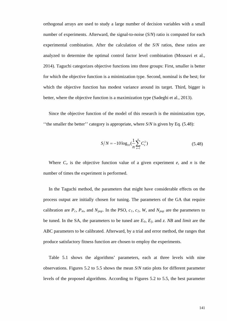
orthogonal arrays are used to study a large number of decision variables with a small
number of experiments. Afterward, the signal-to-noise (S/N) ratio is computed for each
experimental combination. After the calculation of the S/N ratios, these ratios are
analyzed to determine the optimal control factor level combination (Mousavi et al.,
2014). Taguchi categorizes objective functions into three groups: First, smaller is better
for which the objective function is a minimization type. Second, nominal is the best; for
which the objective function has modest variance around its target. Third, bigger is
better, where the objective function is a maximization type (Sadeghi et al., 2013).
Since the objective function of the model of this research is the minimization type,
‘‘the smaller the better’’ category is appropriate, where S/N is given by Eq. (5.48):
210
1
110log ( )n
ee
S N Cn =
= − ∑ (5.48)
Where Ce is the objective function value of a given experiment e, and n is the
number of times the experiment is performed.
In the Taguchi method, the parameters that might have considerable effects on the
process output are initially chosen for tuning. The parameters of the GA that require
calibration are Pc, Pm, and Npop. In the PSO, c1, c2, W, and Npop are the parameters to
be tuned. In the SA, the parameters to be tuned are E0, Ef, and z. NB and limit are the
ABC parameters to be calibrated. Afterward, by a trial and error method, the ranges that
produce satisfactory fitness function are chosen to employ the experiments.
Table 5.1 shows the algorithms’ parameters, each at three levels with nine
observations. Figures 5.2 to 5.5 shows the mean S/N ratio plots for different parameter
levels of the proposed algorithms. According to Figures 5.2 to 5.5, the best parameter
141
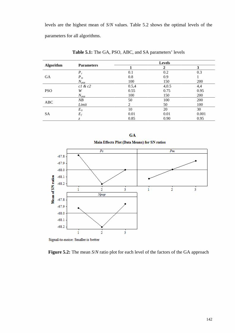
levels are the highest mean of S/N values. Table 5.2 shows the optimal levels of the
parameters for all algorithms.
Table 5.1: The GA, PSO, ABC, and SA parameters’ levels
Algorithm Parameters Levels 1 2 3
GA Pc 0.1 0.2 0.3 Pm 0.8 0.9 1 Npop 100 150 200
PSO c1 & c2 0.5,4 4,0.5 4,4 W 0.55 0.75 0.95 Npop 100 150 200
ABC NB 50 100 200 Limit 2 50 100
SA E0 10 20 30 Ef 0.01 0.01 0.001 z 0.85 0.90 0.95
Figure 5.2: The mean S/N ratio plot for each level of the factors of the GA approach
142
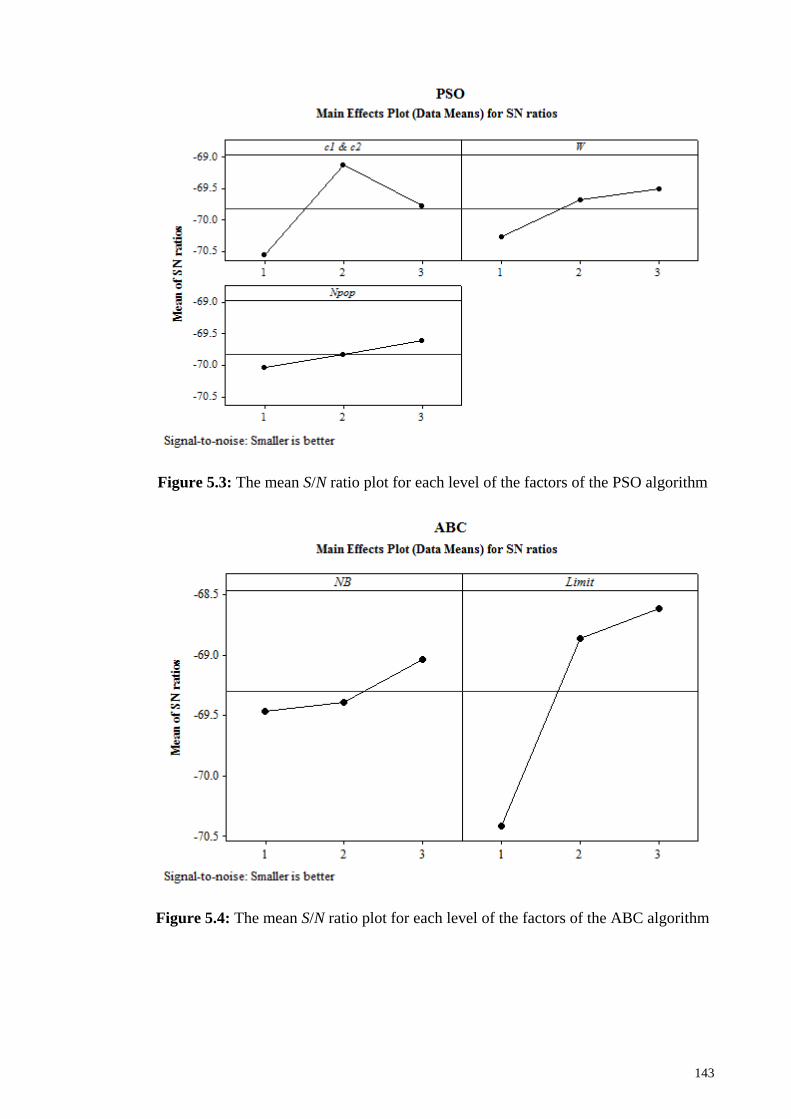
Figure 5.3: The mean S/N ratio plot for each level of the factors of the PSO algorithm
Figure 5.4: The mean S/N ratio plot for each level of the factors of the ABC algorithm
143
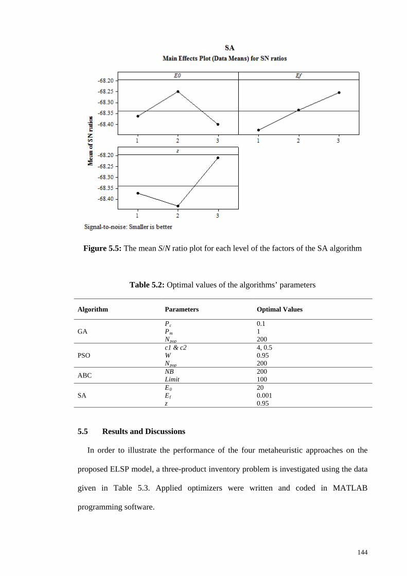
Figure 5.5: The mean S/N ratio plot for each level of the factors of the SA algorithm
Table 5.2: Optimal values of the algorithms’ parameters
Algorithm Parameters Optimal Values
GA Pc 0.1 Pm 1 Npop 200
PSO c1 & c2 4, 0.5 W 0.95 Npop 200
ABC NB 200 Limit 100
SA E0 20 Ef 0.001 z 0.95
5.5 Results and Discussions
In order to illustrate the performance of the four metaheuristic approaches on the
proposed ELSP model, a three-product inventory problem is investigated using the data
given in Table 5.3. Applied optimizers were written and coded in MATLAB
programming software.
144
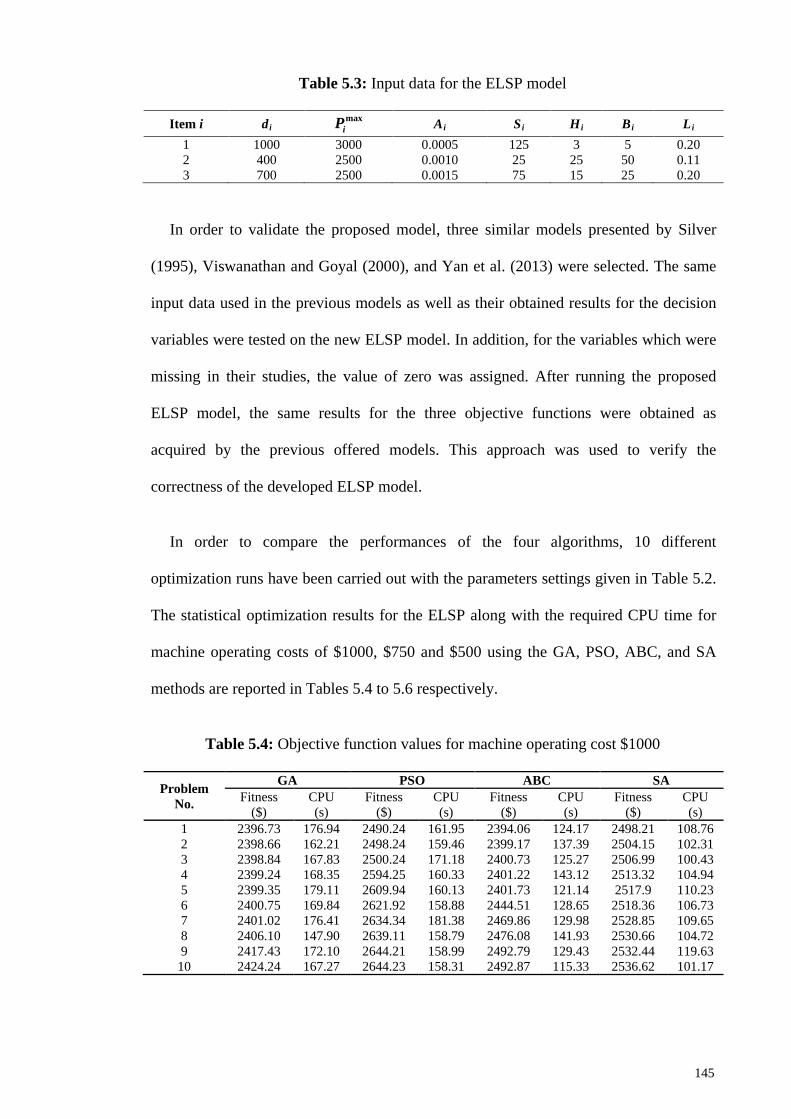
Table 5.3: Input data for the ELSP model
Item i di max
iP Ai Si Hi
Bi Li
1 1000 3000 0.0005 125 3 5 0.20 2 400 2500 0.0010 25 25 50 0.11 3 700 2500 0.0015 75 15 25 0.20
In order to validate the proposed model, three similar models presented by Silver
(1995), Viswanathan and Goyal (2000), and Yan et al. (2013) were selected. The same
input data used in the previous models as well as their obtained results for the decision
variables were tested on the new ELSP model. In addition, for the variables which were
missing in their studies, the value of zero was assigned. After running the proposed
ELSP model, the same results for the three objective functions were obtained as
acquired by the previous offered models. This approach was used to verify the
correctness of the developed ELSP model.
In order to compare the performances of the four algorithms, 10 different
optimization runs have been carried out with the parameters settings given in Table 5.2.
The statistical optimization results for the ELSP along with the required CPU time for
machine operating costs of $1000, $750 and $500 using the GA, PSO, ABC, and SA
methods are reported in Tables 5.4 to 5.6 respectively.
Table 5.4: Objective function values for machine operating cost $1000
Problem No.
GA PSO ABC SA Fitness
($) CPU (s)
Fitness ($)
CPU (s)
Fitness ($)
CPU (s)
Fitness ($)
CPU (s)
1 2396.73 176.94 2490.24 161.95 2394.06 124.17 2498.21 108.76 2 2398.66 162.21 2498.24 159.46 2399.17 137.39 2504.15 102.31 3 2398.84 167.83 2500.24 171.18 2400.73 125.27 2506.99 100.43 4 2399.24 168.35 2594.25 160.33 2401.22 143.12 2513.32 104.94 5 2399.35 179.11 2609.94 160.13 2401.73 121.14 2517.9 110.23 6 2400.75 169.84 2621.92 158.88 2444.51 128.65 2518.36 106.73 7 2401.02 176.41 2634.34 181.38 2469.86 129.98 2528.85 109.65 8 2406.10 147.90 2639.11 158.79 2476.08 141.93 2530.66 104.72 9 2417.43 172.10 2644.21 158.99 2492.79 129.43 2532.44 119.63
10 2424.24 167.27 2644.23 158.31 2492.87 115.33 2536.62 101.17
145
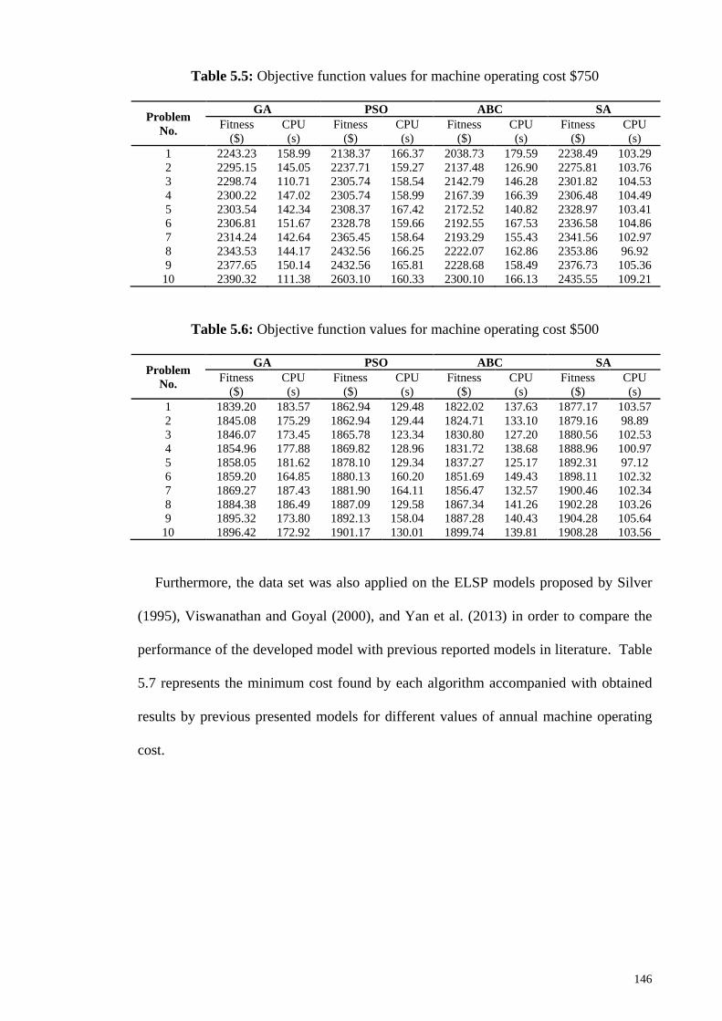
Table 5.5: Objective function values for machine operating cost $750
Problem No.
GA PSO ABC SA Fitness
($) CPU (s)
Fitness ($)
CPU (s)
Fitness ($)
CPU (s)
Fitness ($)
CPU (s)
1 2243.23 158.99 2138.37 166.37 2038.73 179.59 2238.49 103.29 2 2295.15 145.05 2237.71 159.27 2137.48 126.90 2275.81 103.76 3 2298.74 110.71 2305.74 158.54 2142.79 146.28 2301.82 104.53 4 2300.22 147.02 2305.74 158.99 2167.39 166.39 2306.48 104.49 5 2303.54 142.34 2308.37 167.42 2172.52 140.82 2328.97 103.41 6 2306.81 151.67 2328.78 159.66 2192.55 167.53 2336.58 104.86 7 2314.24 142.64 2365.45 158.64 2193.29 155.43 2341.56 102.97 8 2343.53 144.17 2432.56 166.25 2222.07 162.86 2353.86 96.92 9 2377.65 150.14 2432.56 165.81 2228.68 158.49 2376.73 105.36
10 2390.32 111.38 2603.10 160.33 2300.10 166.13 2435.55 109.21
Table 5.6: Objective function values for machine operating cost $500
Problem No.
GA PSO ABC SA Fitness
($) CPU (s)
Fitness ($)
CPU (s)
Fitness ($)
CPU (s)
Fitness ($)
CPU (s)
1 1839.20 183.57 1862.94 129.48 1822.02 137.63 1877.17 103.57 2 1845.08 175.29 1862.94 129.44 1824.71 133.10 1879.16 98.89 3 1846.07 173.45 1865.78 123.34 1830.80 127.20 1880.56 102.53 4 1854.96 177.88 1869.82 128.96 1831.72 138.68 1888.96 100.97 5 1858.05 181.62 1878.10 129.34 1837.27 125.17 1892.31 97.12 6 1859.20 164.85 1880.13 160.20 1851.69 149.43 1898.11 102.32 7 1869.27 187.43 1881.90 164.11 1856.47 132.57 1900.46 102.34 8 1884.38 186.49 1887.09 129.58 1867.34 141.26 1902.28 103.26 9 1895.32 173.80 1892.13 158.04 1887.28 140.43 1904.28 105.64
10 1896.42 172.92 1901.17 130.01 1899.74 139.81 1908.28 103.56
Furthermore, the data set was also applied on the ELSP models proposed by Silver
(1995), Viswanathan and Goyal (2000), and Yan et al. (2013) in order to compare the
performance of the developed model with previous reported models in literature. Table
5.7 represents the minimum cost found by each algorithm accompanied with obtained
results by previous presented models for different values of annual machine operating
cost.
146
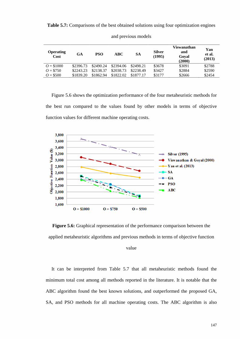
Table 5.7: Comparisons of the best obtained solutions using four optimization engines
and previous models
Operating Cost GA PSO ABC SA Silver
(1995)
Viswanathan and
Goyal (2000)
Yan et al.
(2013)
O = $1000 $2396.73 $2490.24 $2394.06 $2498.21 $3678 $3091 $2788 O = $750 $2243.23 $2138.37 $2038.73 $2238.49 $3427 $2884 $2590 O = $500 $1839.20 $1862.94 $1822.02 $1877.17 $3177 $2666 $2454
Figure 5.6 shows the optimization performance of the four metaheuristic methods for
the best run compared to the values found by other models in terms of objective
function values for different machine operating costs.
Figure 5.6: Graphical representation of the performance comparison between the
applied metaheuristic algorithms and previous methods in terms of objective function
value
It can be interpreted from Table 5.7 that all metaheuristic methods found the
minimum total cost among all methods reported in the literature. It is notable that the
ABC algorithm found the best known solutions, and outperformed the proposed GA,
SA, and PSO methods for all machine operating costs. The ABC algorithm is also
147
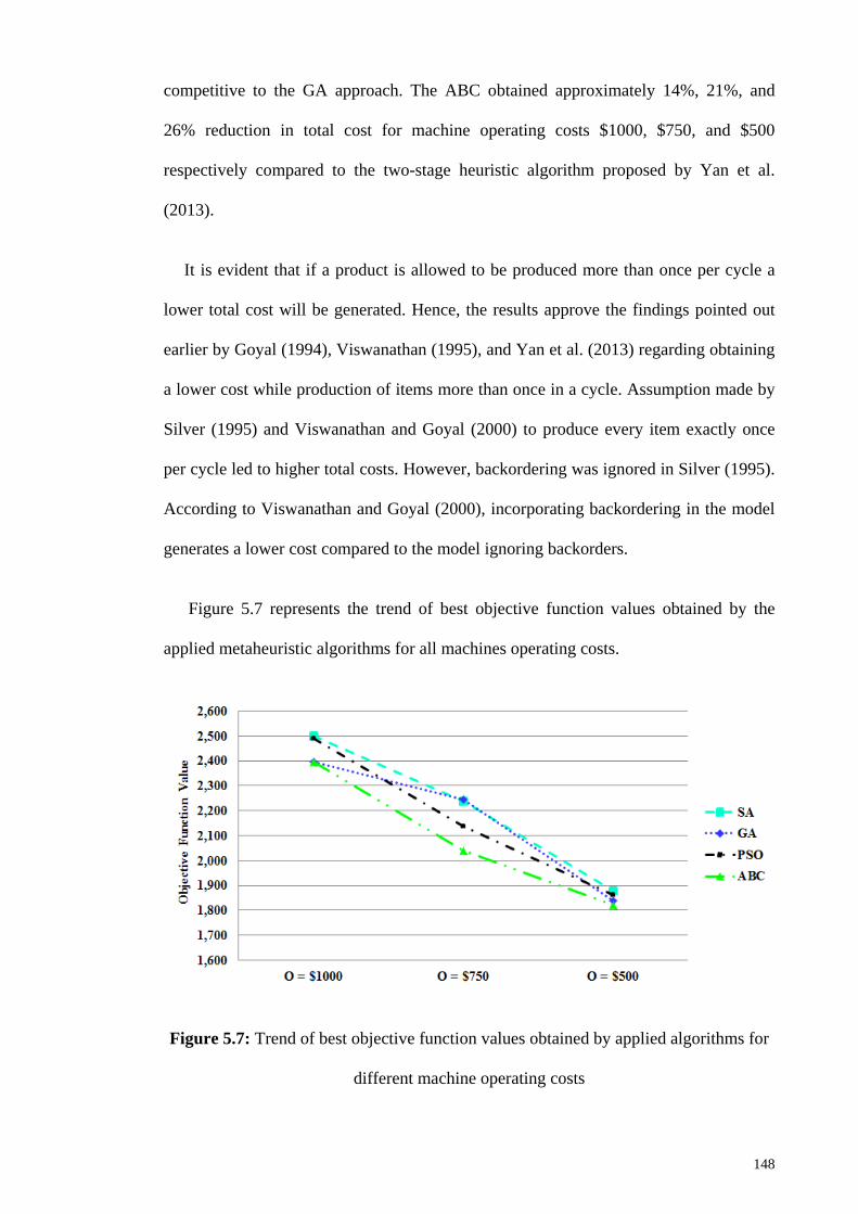
competitive to the GA approach. The ABC obtained approximately 14%, 21%, and
26% reduction in total cost for machine operating costs $1000, $750, and $500
respectively compared to the two-stage heuristic algorithm proposed by Yan et al.
(2013).
It is evident that if a product is allowed to be produced more than once per cycle a
lower total cost will be generated. Hence, the results approve the findings pointed out
earlier by Goyal (1994), Viswanathan (1995), and Yan et al. (2013) regarding obtaining
a lower cost while production of items more than once in a cycle. Assumption made by
Silver (1995) and Viswanathan and Goyal (2000) to produce every item exactly once
per cycle led to higher total costs. However, backordering was ignored in Silver (1995).
According to Viswanathan and Goyal (2000), incorporating backordering in the model
generates a lower cost compared to the model ignoring backorders.
Figure 5.7 represents the trend of best objective function values obtained by the
applied metaheuristic algorithms for all machines operating costs.
Figure 5.7: Trend of best objective function values obtained by applied algorithms for
different machine operating costs
148

Figure 5.8 shows the performance of four metaheuristic approaches in terms of
objective function values for machine operating cost $1000 in 10 runs. The figure
shows that the ABC and GA performed better than PSO and SA.
Figure 5.8: Comparison of applied metaheuristics in terms of objective function value
for machine operating cost $1000
The computation time (CPU time) of applied metaheuristics for machine operating
cost $1000 in 10 runs is illustrated in Figure 5.9.
Figure 5.9: Comparison of applied metaheuristics in terms of CPU time for machine
operating cost $1000
149
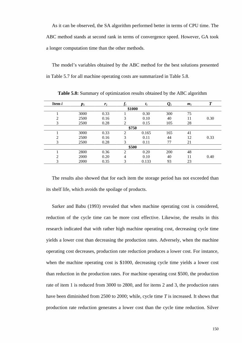
As it can be observed, the SA algorithm performed better in terms of CPU time. The
ABC method stands at second rank in terms of convergence speed. However, GA took
a longer computation time than the other methods.
The model’s variables obtained by the ABC method for the best solutions presented
in Table 5.7 for all machine operating costs are summarized in Table 5.8.
Table 5.8: Summary of optimization results obtained by the ABC algorithm
Item i pi ri
fi ti
Qi mi
T $1000
1 3000 0.33 1 0.30 300 75 0.30 2 2500 0.16 3 0.10 40 11
3 2500 0.28 2 0.15 105 28 $750
1 3000 0.33 2 0.165 165 41 0.33 2 2500 0.16 3 0.11 44 12
3 2500 0.28 3 0.11 77 21 $500
1 2800 0.36 2 0.20 200 48 0.40 2 2000 0.20 4 0.10 40 11
3 2000 0.35 3 0.133 93 23
The results also showed that for each item the storage period has not exceeded than
its shelf life, which avoids the spoilage of products.
Sarker and Babu (1993) revealed that when machine operating cost is considered,
reduction of the cycle time can be more cost effective. Likewise, the results in this
research indicated that with rather high machine operating cost, decreasing cycle time
yields a lower cost than decreasing the production rates. Adversely, when the machine
operating cost decreases, production rate reduction produces a lower cost. For instance,
when the machine operating cost is $1000, decreasing cycle time yields a lower cost
than reduction in the production rates. For machine operating cost $500, the production
rate of item 1 is reduced from 3000 to 2800, and for items 2 and 3, the production rates
have been diminished from 2500 to 2000; while, cycle time T is increased. It shows that
production rate reduction generates a lower cost than the cycle time reduction. Silver
150
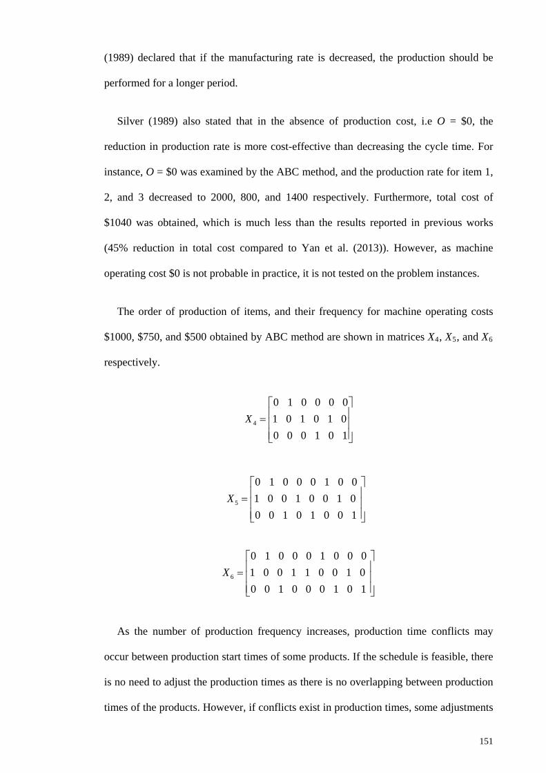
(1989) declared that if the manufacturing rate is decreased, the production should be
performed for a longer period.
Silver (1989) also stated that in the absence of production cost, i.e O = $0, the
reduction in production rate is more cost-effective than decreasing the cycle time. For
instance, O = $0 was examined by the ABC method, and the production rate for item 1,
2, and 3 decreased to 2000, 800, and 1400 respectively. Furthermore, total cost of
$1040 was obtained, which is much less than the results reported in previous works
(45% reduction in total cost compared to Yan et al. (2013)). However, as machine
operating cost $0 is not probable in practice, it is not tested on the problem instances.
The order of production of items, and their frequency for machine operating costs
$1000, $750, and $500 obtained by ABC method are shown in matrices X4, X5, and X6
respectively.
4
0 1 0 0 0 01 0 1 0 1 00 0 0 1 0 1
X =
6
0 1 0 0 0 1 0 0 0 1 0 0 1 1 0 0 1 00 0 1 0 0 0 1 0 1
X =
As the number of production frequency increases, production time conflicts may
occur between production start times of some products. If the schedule is feasible, there
is no need to adjust the production times as there is no overlapping between production
times of the products. However, if conflicts exist in production times, some adjustments
5
0 1 0 0 0 1 0 0 1 0 0 1 0 0 1 00 0 1 0 1 0 0 1
X =
151
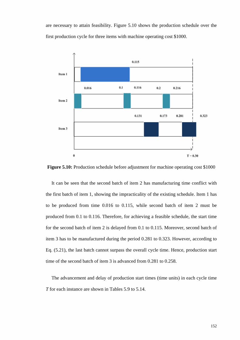
are necessary to attain feasibility. Figure 5.10 shows the production schedule over the
first production cycle for three items with machine operating cost $1000.
Figure 5.10: Production schedule before adjustment for machine operating cost $1000
It can be seen that the second batch of item 2 has manufacturing time conflict with
the first batch of item 1, showing the impracticality of the existing schedule. Item 1 has
to be produced from time 0.016 to 0.115, while second batch of item 2 must be
produced from 0.1 to 0.116. Therefore, for achieving a feasible schedule, the start time
for the second batch of item 2 is delayed from 0.1 to 0.115. Moreover, second batch of
item 3 has to be manufactured during the period 0.281 to 0.323. However, according to
Eq. (5.21), the last batch cannot surpass the overall cycle time. Hence, production start
time of the second batch of item 3 is advanced from 0.281 to 0.258.
The advancement and delay of production start times (time units) in each cycle time
T for each instance are shown in Tables 5.9 to 5.14.
152
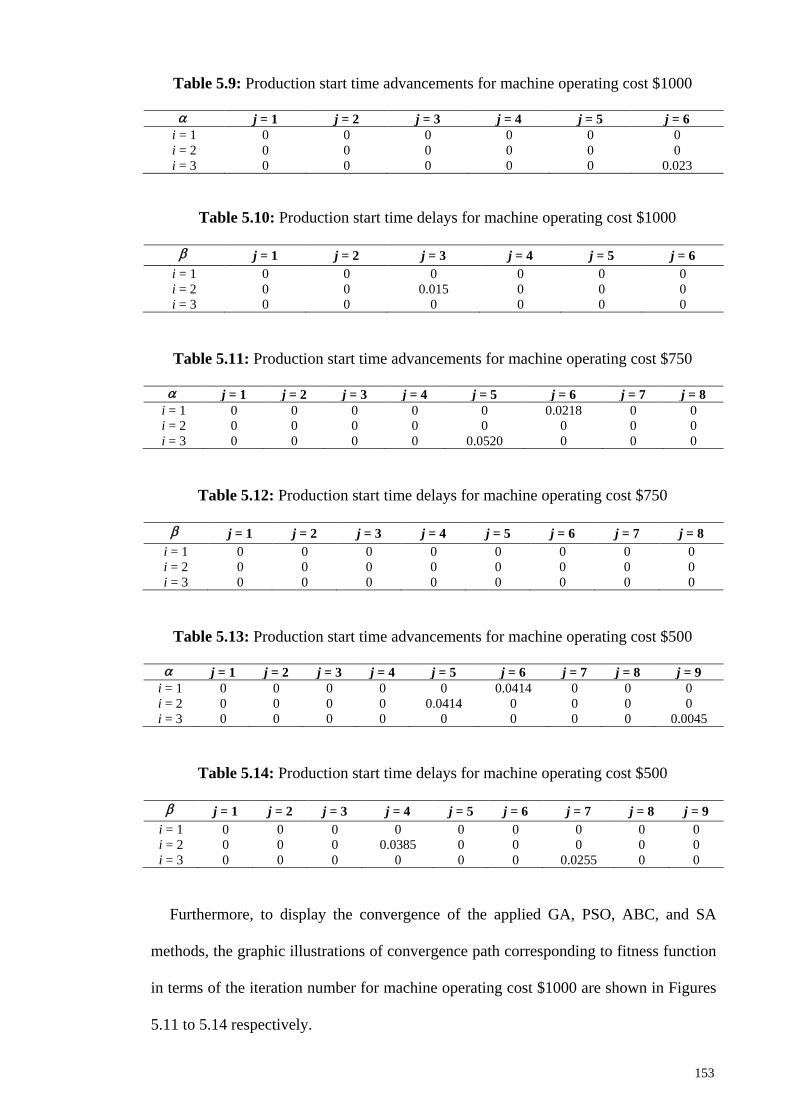
Table 5.9: Production start time advancements for machine operating cost $1000
α j = 1 j = 2 j = 3 j = 4 j = 5 j = 6
i = 1 0 0 0 0 0 0 i = 2 0 0 0 0 0 0 i = 3 0 0 0 0 0 0.023
Table 5.10: Production start time delays for machine operating cost $1000
β j = 1 j = 2 j = 3 j = 4 j = 5 j = 6
i = 1 0 0 0 0 0 0 i = 2 0 0 0.015 0 0 0 i = 3 0 0 0 0 0 0
Table 5.11: Production start time advancements for machine operating cost $750
α j = 1 j = 2 j = 3 j = 4 j = 5 j = 6 j = 7 j = 8
i = 1 0 0 0 0 0 0.0218 0 0 i = 2 0 0 0 0 0 0 0 0 i = 3 0 0 0 0 0.0520 0 0 0
Table 5.12: Production start time delays for machine operating cost $750
β j = 1 j = 2 j = 3 j = 4 j = 5 j = 6 j = 7 j = 8
i = 1 0 0 0 0 0 0 0 0 i = 2 0 0 0 0 0 0 0 0 i = 3 0 0 0 0 0 0 0 0
Table 5.13: Production start time advancements for machine operating cost $500
α j = 1 j = 2 j = 3 j = 4 j = 5 j = 6 j = 7 j = 8 j = 9
i = 1 0 0 0 0 0 0.0414 0 0 0 i = 2 0 0 0 0 0.0414 0 0 0 0 i = 3 0 0 0 0 0 0 0 0 0.0045
Table 5.14: Production start time delays for machine operating cost $500
β j = 1 j = 2 j = 3 j = 4 j = 5 j = 6 j = 7 j = 8 j = 9
i = 1 0 0 0 0 0 0 0 0 0 i = 2 0 0 0 0.0385 0 0 0 0 0 i = 3 0 0 0 0 0 0 0.0255 0 0
Furthermore, to display the convergence of the applied GA, PSO, ABC, and SA
methods, the graphic illustrations of convergence path corresponding to fitness function
in terms of the iteration number for machine operating cost $1000 are shown in Figures
5.11 to 5.14 respectively.
153
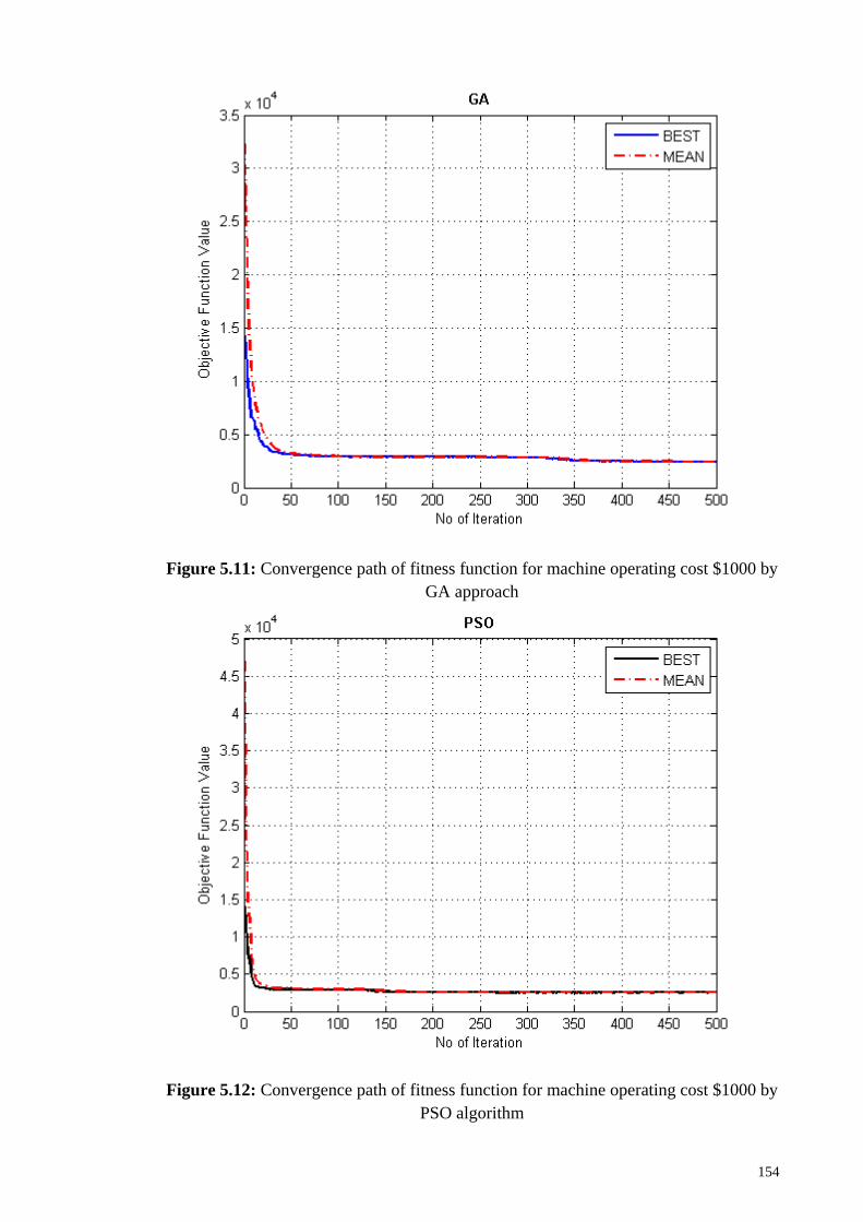
Figure 5.11: Convergence path of fitness function for machine operating cost $1000 by GA approach
Figure 5.12: Convergence path of fitness function for machine operating cost $1000 by PSO algorithm
154
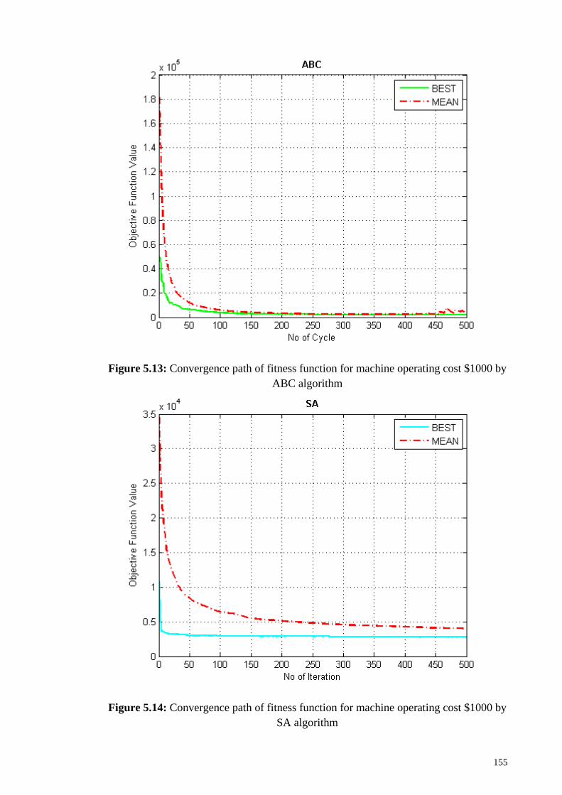
Figure 5.13: Convergence path of fitness function for machine operating cost $1000 by ABC algorithm
Figure 5.14: Convergence path of fitness function for machine operating cost $1000 by SA algorithm
155
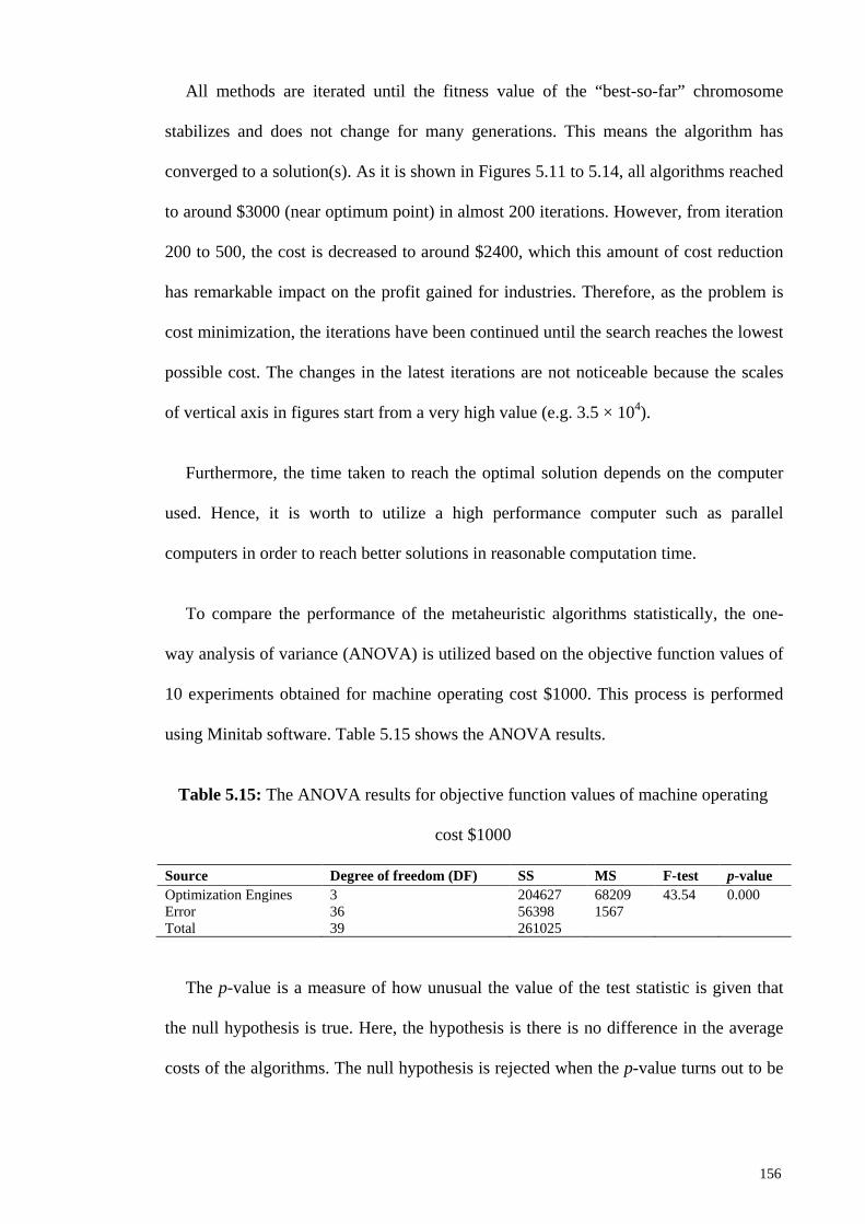
All methods are iterated until the fitness value of the “best-so-far” chromosome
stabilizes and does not change for many generations. This means the algorithm has
converged to a solution(s). As it is shown in Figures 5.11 to 5.14, all algorithms reached
to around $3000 (near optimum point) in almost 200 iterations. However, from iteration
200 to 500, the cost is decreased to around $2400, which this amount of cost reduction
has remarkable impact on the profit gained for industries. Therefore, as the problem is
cost minimization, the iterations have been continued until the search reaches the lowest
possible cost. The changes in the latest iterations are not noticeable because the scales
of vertical axis in figures start from a very high value (e.g. 3.5 × 10⁴).
Furthermore, the time taken to reach the optimal solution depends on the computer
used. Hence, it is worth to utilize a high performance computer such as parallel
computers in order to reach better solutions in reasonable computation time.
To compare the performance of the metaheuristic algorithms statistically, the one-
way analysis of variance (ANOVA) is utilized based on the objective function values of
10 experiments obtained for machine operating cost $1000. This process is performed
using Minitab software. Table 5.15 shows the ANOVA results.
Table 5.15: The ANOVA results for objective function values of machine operating
cost $1000
Source Degree of freedom (DF) SS MS F-test p-value Optimization Engines 3 204627 68209 43.54 0.000 Error 36 56398 1567 Total 39 261025
The p-value is a measure of how unusual the value of the test statistic is given that
the null hypothesis is true. Here, the hypothesis is there is no difference in the average
costs of the algorithms. The null hypothesis is rejected when the p-value turns out to be
156
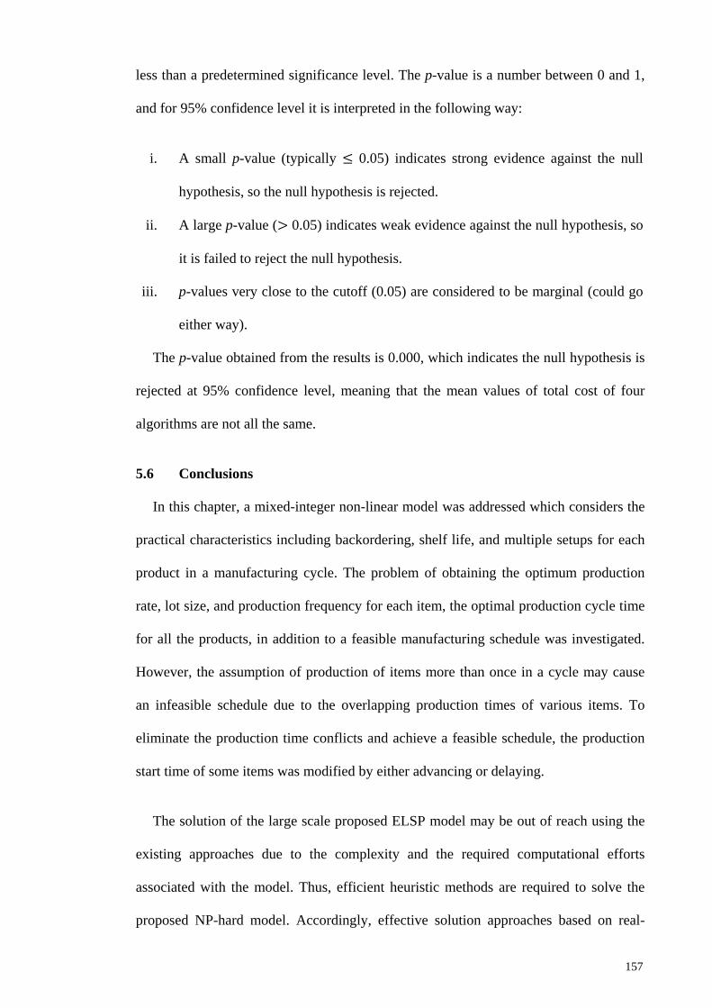
less than a predetermined significance level. The p-value is a number between 0 and 1,
and for 95% confidence level it is interpreted in the following way:
i. A small p-value (typically ≤ 0.05) indicates strong evidence against the null
hypothesis, so the null hypothesis is rejected.
ii. A large p-value (> 0.05) indicates weak evidence against the null hypothesis, so
it is failed to reject the null hypothesis.
iii. p-values very close to the cutoff (0.05) are considered to be marginal (could go
either way).
The p-value obtained from the results is 0.000, which indicates the null hypothesis is
rejected at 95% confidence level, meaning that the mean values of total cost of four
algorithms are not all the same.
5.6 Conclusions
In this chapter, a mixed-integer non-linear model was addressed which considers the
practical characteristics including backordering, shelf life, and multiple setups for each
product in a manufacturing cycle. The problem of obtaining the optimum production
rate, lot size, and production frequency for each item, the optimal production cycle time
for all the products, in addition to a feasible manufacturing schedule was investigated.
However, the assumption of production of items more than once in a cycle may cause
an infeasible schedule due to the overlapping production times of various items. To
eliminate the production time conflicts and achieve a feasible schedule, the production
start time of some items was modified by either advancing or delaying.
The solution of the large scale proposed ELSP model may be out of reach using the
existing approaches due to the complexity and the required computational efforts
associated with the model. Thus, efficient heuristic methods are required to solve the
proposed NP-hard model. Accordingly, effective solution approaches based on real-
157
coded GA, PSO, ABC, and SA algorithms for integer, non-integer, and binary variables
were presented to solve the model. Furthermore, to make the algorithms more effective,
Taguchi method was employed to tune various parameters of the applied algorithms.
Each of such methods was applied to a set of problem instances taken from literature
and the performances were compared against other existing models in the literature. The
results indicated the efficiency of the applied metaheuristic algorithms in solving the
proposed model. Comparisons were based on the percentage improvement in the total
cost. All the applied methods showed an impressive performance and excellent solution
qualities. The metaheuristic algorithms can also efficiently handle large-sized instances
in a moderate computation time. Based on the results, the ABC algorithm produced the
lowest cost, which may indicate its superiority in searching for optimal solutions of
similar problems.
158
CHAPTER 6: OPTIMIZATION OF MULTI-PLANT CAPACITATED LOT-
SIZING PROBLEM IN AN INTEGRATED PRODUCTION-DISTRIBUTION
NETWORK USING CALIBRATED METAHEURISTIC ALGORITHMS
6.1 Introduction
In this chapter, the multi-item, multi-period, multi-plant capacitated lot-sizing
problem with inter-plant interactions, multiple suppliers and distribution centers is
addressed, which can cover a variety of problems arising in the literature and in
practice. The fundamental concept is to simultaneously optimize decision variables of
different functions in a supply chain that have been conventionally optimized
individually due to the complexity in their integration. The combinations of several
functions such as purchasing, production, storage, backordering, and transportation are
considered to evaluate the impact of coordination on the cost performance of a multi-
plant firm. A number of well-known metaheuristic algorithms are utilized to solve the
proposed model.
The subsequent sections of this chapter are organized as follow: Section 6.2 presents
the mathematical formulation for the proposed problem. In Section 6.3, metaheuristic
algorithms namely the GA, PSO, ABC, and ICA are presented to solve the proposed
model. Section 6.4 demonstrates the numerical example. Section 6.5 explains the
parameter calibration procedure using the Taguchi method. In Section 6.6 the
computational results are discusses. Finally, the conclusions are shared in Section 6.7.
6.2 Problem Description and Mathematical Formulations
The considered production and distribution planning problem consists of M
suppliers, J plants, and W distribution centers, as shown in Figure 6.1. It is assumed that
production takes place in a multi-plant manufacturing company, where the plants are
geographically distributed in different locations of a country. Each product is made of K
159
raw materials which are provided by the suppliers. It is designated that for each raw
material type there is only one particular supplier. Each plant is characterized by its own
inventory and production capacities. It is possible to store excess production at the plant
storage which has capacity limit, but no storage is possible for end products at
distribution centers.
Any of the products produced in each plant can be transported to any of the
distribution centers that are located in different areas. Obviously, the demand in a
distribution centre is served by the closest plant. Transfer decisions between plants are
made when demand observed at a plant can be satisfied by other production sites to
cope with under-capacity of that particular plant. It should be noted that the customer
would pay only for the transportation from the nearest plant. The transportation cost
from other plants to the plant where demand has been placed, has to be borne by the
company.
Since all factories, suppliers and distribution centers are spread out geographically,
the transportation cost can vary. Homogenous vehicles of a given capacity are stationed
at each supplier and plant to deliver products from suppliers to plants, between the
production plants, and from plants to distribution centers. The model is developed with
the assumption that sales are made at the distribution centers. In addition, backordering
is allowed when demand at a distribution centre cannot be entirely satisfied.
160
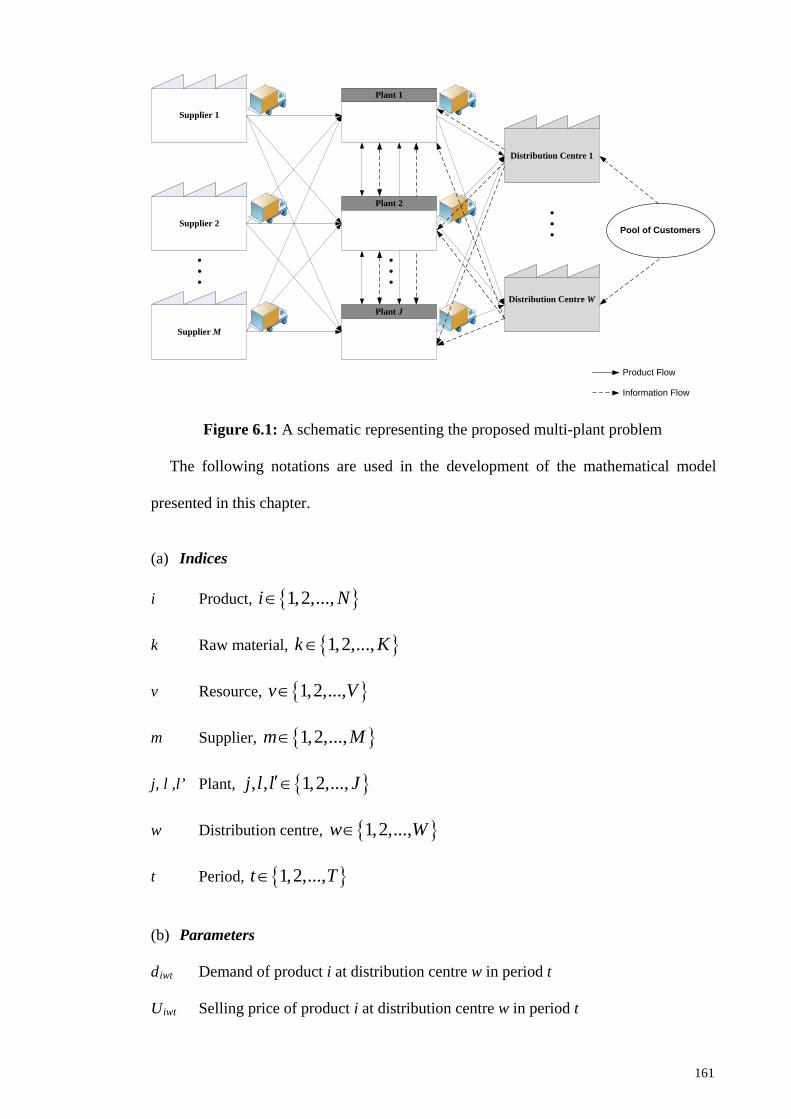
• • •
Supplier 1
Supplier 2
Supplier M
Plant 1
Plant J
Plant 2
Distribution Centre 1
Distribution Centre W
Pool of Customers
Product Flow
Information Flow
• • •
• • •
Figure 6.1: A schematic representing the proposed multi-plant problem
The following notations are used in the development of the mathematical model
presented in this chapter.
(a) Indices
i Product, 1,2,...,i N∈
k Raw material, 1,2,...,k K∈
v Resource, 1,2,...,v V∈
m Supplier, 1,2,...,m M∈
j, l ,l’ Plant, , , 1,2,...,j l l J′∈
w Distribution centre, 1,2,...,w W∈
t Period, 1,2,...,t T∈
(b) Parameters
diwt Demand of product i at distribution centre w in period t
Uiwt Selling price of product i at distribution centre w in period t
161

Aijt Setup time of product i at plant j in period t
Pijt Production time of product i at plant j in period t
Fjt Total available production time at plant j in period t
xki Amount of raw material k required to produce a unit of product i
Ekmt Number of raw material k that can be provided by supplier m in period t
kmjtλ Percentage of rejected raw material k delivered by supplier m to plant j in period
t
Rvij Amount of resource v required to produce a unit of product i at plant j
Nvjt Total amount of resource v available at plant j in period t
kmtπ Ordering cost of raw material k at supplier m in period t
kmtτ Purchasing cost of raw material k at supplier m in period t
Sijt Setup cost for product i at plant j in period t
Oijt Production cost of product i at plant j in period t
Hkjt Holding cost of raw material k at plant j in period t
ijtH ′ Holding cost of product i at plant j in period t
Biwt Backordering cost of product i at distribution centre w in period t
mjϖ Distance between supplier m and plant j
jlµ Distance between plant j and plant l
jwζ Distance between plant j and distribution centre w
kjσ
Storage capacity for raw material k at plant j
ijσ ′
Storage capacity for item i at plant j
kς Vehicle available capacity respect to raw material k
iς ′ Vehicle available capacity respect to product i
Fη Fixed transportation cost of vehicle
162
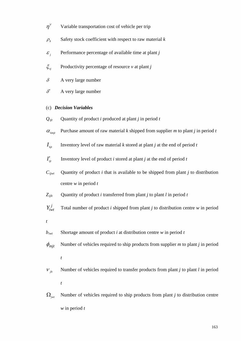
Vη Variable transportation cost of vehicle per trip
kρ Safety stock coefficient with respect to raw material k
jε Performance percentage of available time at plant j
vjξ Productivity percentage of resource v at plant j
δ A very large number
δ ′ A very large number
(c) Decision Variables
Qijt Quantity of product i produced at plant j in period t
kmjtα
Purchase amount of raw material k shipped from supplier m to plant j in period t
kjtI
Inventory level of raw material k stored at plant j at the end of period t
ijtI ′ Inventory level of product i stored at plant j at the end of period t
Cijwt Quantity of product i that is available to be shipped from plant j to distribution
centre w in period t
Zijlt Quantity of product i transferred from plant j to plant l in period t
jiwtY Total number of product i shipped from plant j to distribution centre w in period
t
biwt Shortage amount of product i at distribution centre w in period t
mjtφ Number of vehicles required to ship products from supplier m to plant j in period
t
jltν Number of vehicles required to transfer products from plant j to plant l in period
t
jwtΩ Number of vehicles required to ship products from plant j to distribution centre
w in period t
163
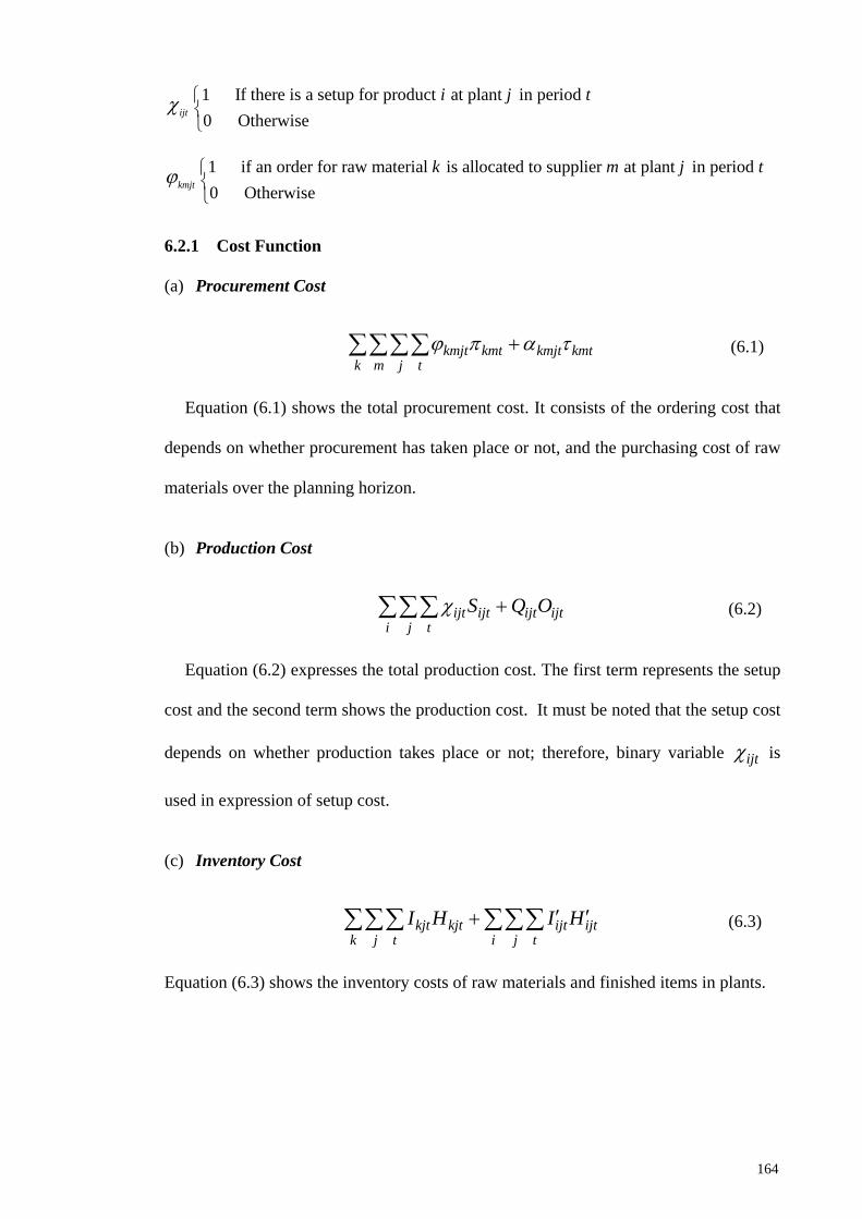
ijtχ 1 If there is a setup for product at plant in period 0 Otherwise
i j t
kmjtϕ 1 if an order for raw material is allocated to supplier at plant in period 0 Otherwise
k m j t
6.2.1 Cost Function
(a) Procurement Cost
kmjt kmt kmjt kmtk m j t
ϕ π α τ+∑∑∑∑ (6.1)
Equation (6.1) shows the total procurement cost. It consists of the ordering cost that
depends on whether procurement has taken place or not, and the purchasing cost of raw
materials over the planning horizon.
(b) Production Cost
ijt ijt ijt ijti j t
S Q Oχ +∑∑∑ (6.2)
Equation (6.2) expresses the total production cost. The first term represents the setup
cost and the second term shows the production cost. It must be noted that the setup cost
depends on whether production takes place or not; therefore, binary variable ijtχ is
used in expression of setup cost.
(c) Inventory Cost
kjt kjt ijt ijtk j t i j t
I H I H′ ′+∑∑∑ ∑∑∑ (6.3)
Equation (6.3) shows the inventory costs of raw materials and finished items in plants.
164
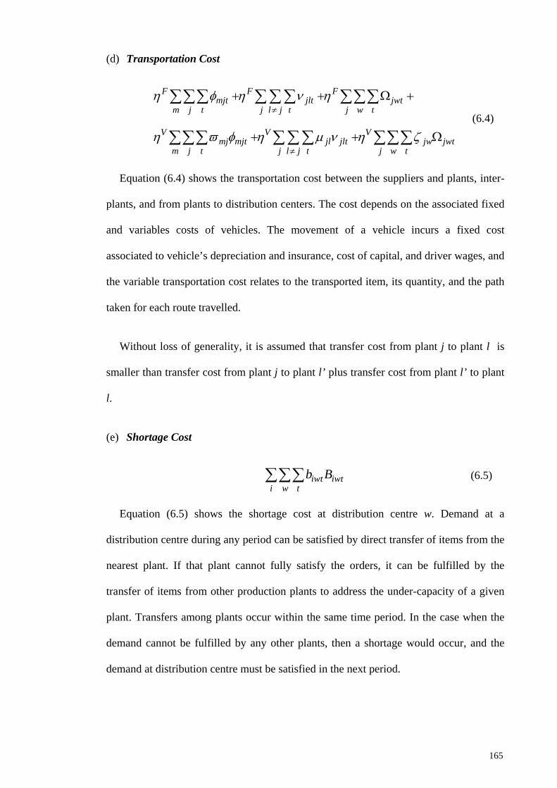
(d) Transportation Cost
F F Fmjt jlt jwt
m j t j l j t j w t
V V Vmj mjt jl jlt jw jwt
m j t j l j t j w t
η φ η ν η
η ϖ φ η µ ν η ζ
≠
≠
+ + Ω +
+ + Ω
∑∑∑ ∑ ∑ ∑ ∑∑∑
∑∑∑ ∑ ∑ ∑ ∑∑∑ (6.4)
Equation (6.4) shows the transportation cost between the suppliers and plants, inter-
plants, and from plants to distribution centers. The cost depends on the associated fixed
and variables costs of vehicles. The movement of a vehicle incurs a fixed cost
associated to vehicle’s depreciation and insurance, cost of capital, and driver wages, and
the variable transportation cost relates to the transported item, its quantity, and the path
taken for each route travelled.
Without loss of generality, it is assumed that transfer cost from plant j to plant l is
smaller than transfer cost from plant j to plant l’ plus transfer cost from plant l’ to plant
l.
(e) Shortage Cost
iwt iwti w t
b B∑∑∑ (6.5)
Equation (6.5) shows the shortage cost at distribution centre w. Demand at a
distribution centre during any period can be satisfied by direct transfer of items from the
nearest plant. If that plant cannot fully satisfy the orders, it can be fulfilled by the
transfer of items from other production plants to address the under-capacity of a given
plant. Transfers among plants occur within the same time period. In the case when the
demand cannot be fulfilled by any other plants, then a shortage would occur, and the
demand at distribution centre must be satisfied in the next period.
165
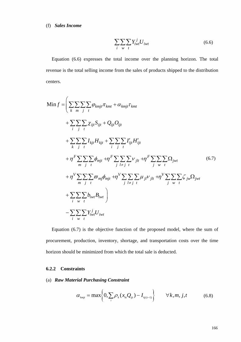
(f) Sales Income
jiwt iwt
i w tY U∑∑∑ (6.6)
Equation (6.6) expresses the total income over the planning horizon. The total
revenue is the total selling income from the sales of products shipped to the distribution
centers.
Min kmjt kmt kmjt kmtk m j t
ijt ijt ijt ijti j t
kjt kjt ijt ijtk j t i j t
F F Fmjt jlt jwt
m j t j l j t j w t
V V Vmj mjt jl jlt jw jwt
m j t j l j t j w t
iwt iwti w t
f
S Q O
I H I H
b B
ϕ π α τ
χ
η φ η ν η
η ϖ φ η µ ν η ζ
≠
≠
= +
+ +
′ ′+ +
+ + + Ω
+ + + Ω
+
∑∑∑∑
∑∑∑
∑∑∑ ∑∑∑
∑∑∑ ∑ ∑ ∑ ∑∑∑
∑∑∑ ∑ ∑ ∑ ∑∑∑
∑∑∑
jiwt iwt
i w tY U
− ∑∑∑
(6.7)
Equation (6.7) is the objective function of the proposed model, where the sum of
procurement, production, inventory, shortage, and transportation costs over the time
horizon should be minimized from which the total sale is deducted.
6.2.2 Constraints
(a) Raw Material Purchasing Constraint
( 1)max 0, ( ) , , ,kmjt k ki ijt kj t
ix Q I k m j tα ρ −= − ∀∑ (6.8)
166
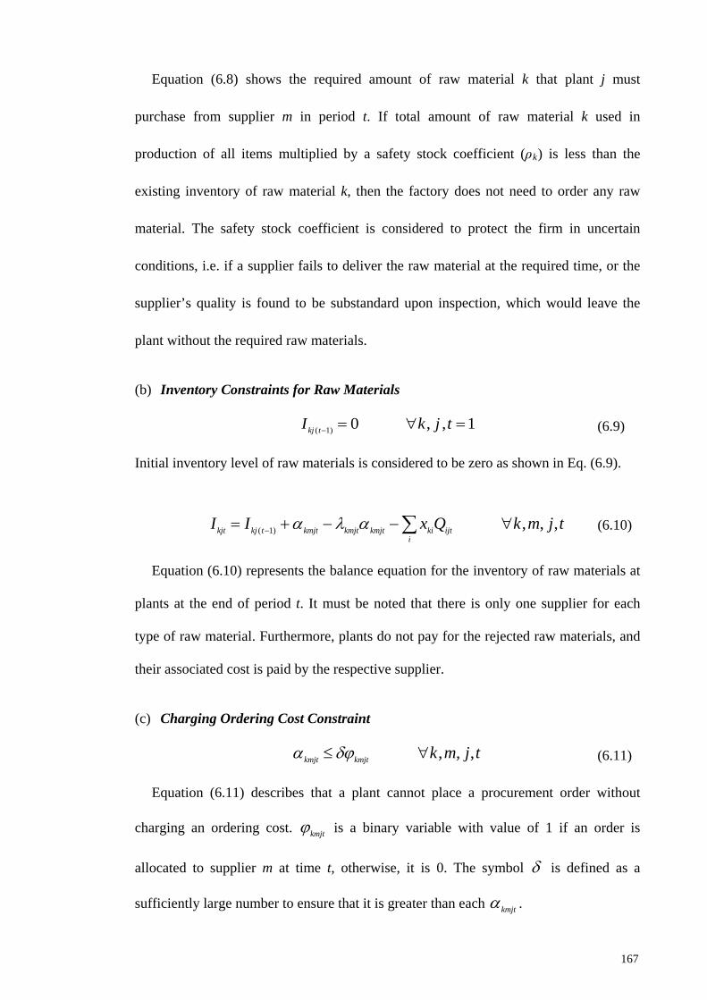
Equation (6.8) shows the required amount of raw material k that plant j must
purchase from supplier m in period t. If total amount of raw material k used in
production of all items multiplied by a safety stock coefficient (ρk) is less than the
existing inventory of raw material k, then the factory does not need to order any raw
material. The safety stock coefficient is considered to protect the firm in uncertain
conditions, i.e. if a supplier fails to deliver the raw material at the required time, or the
supplier’s quality is found to be substandard upon inspection, which would leave the
plant without the required raw materials.
(b) Inventory Constraints for Raw Materials
( 1) 0 , , 1kj tI k j t− = ∀ = (6.9)
Initial inventory level of raw materials is considered to be zero as shown in Eq. (6.9).
( 1) , , ,kjt kj t kmjt kmjt kmjt ki ijti
I I x Q k m j t−= + − − ∀∑α λ α (6.10)
Equation (6.10) represents the balance equation for the inventory of raw materials at
plants at the end of period t. It must be noted that there is only one supplier for each
type of raw material. Furthermore, plants do not pay for the rejected raw materials, and
their associated cost is paid by the respective supplier.
(c) Charging Ordering Cost Constraint
, , ,kmjt kmjt k m j tα δϕ≤ ∀ (6.11)
Equation (6.11) describes that a plant cannot place a procurement order without
charging an ordering cost. kmjtϕ is a binary variable with value of 1 if an order is
allocated to supplier m at time t, otherwise, it is 0. The symbol δ is defined as a
sufficiently large number to ensure that it is greater than each kmjtα .
167
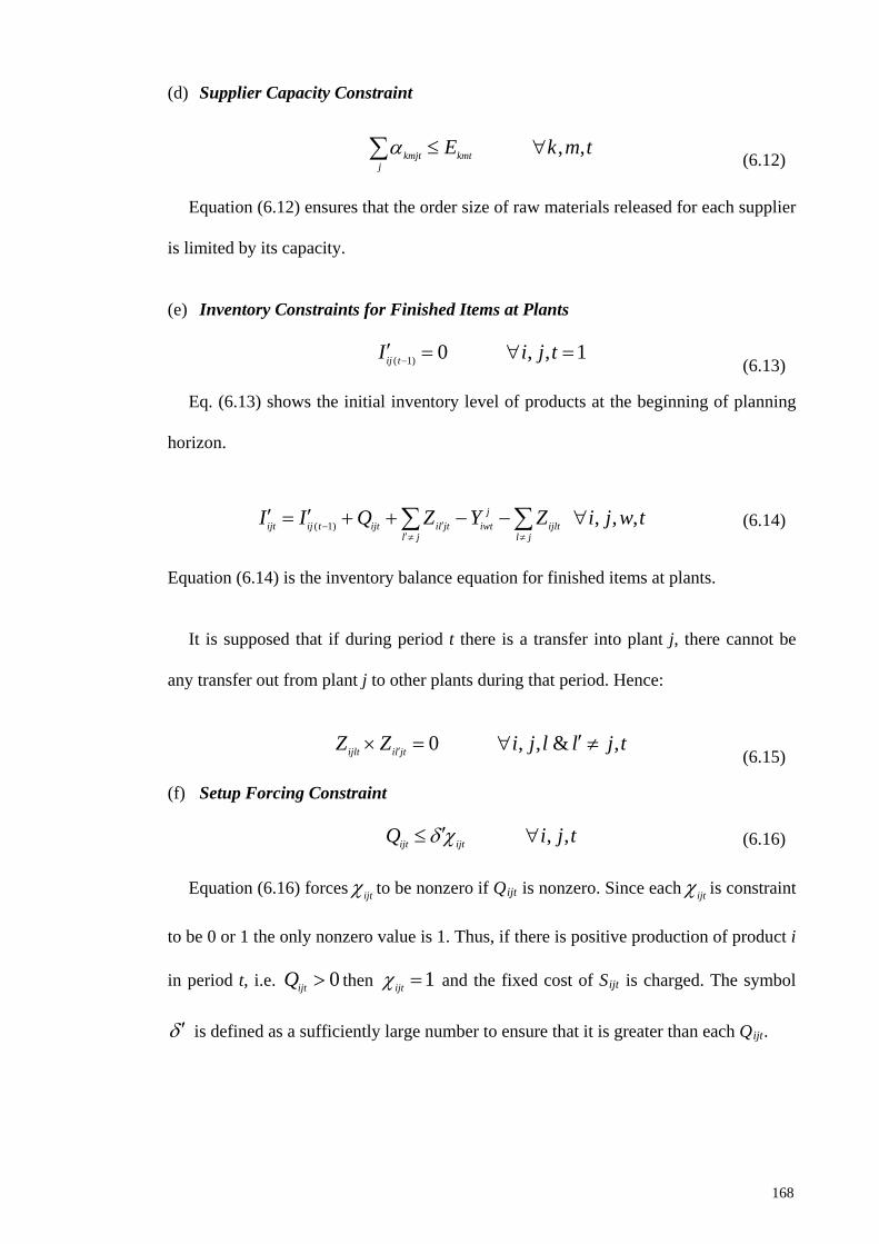
(d) Supplier Capacity Constraint
, ,kmjt kmtj
E k m tα ≤ ∀∑
(6.12)
Equation (6.12) ensures that the order size of raw materials released for each supplier
is limited by its capacity.
(e) Inventory Constraints for Finished Items at Plants
( 1) 0 , , 1ij tI i j t−′ = ∀ =
(6.13)
Eq. (6.13) shows the initial inventory level of products at the beginning of planning
horizon.
( 1) , , ,jijt ij t ijt il jt iwt ijlt
l j l jI I Q Z Y Z i j w t′−
′≠ ≠
′ ′= + + − − ∀∑ ∑ (6.14)
Equation (6.14) is the inventory balance equation for finished items at plants.
It is supposed that if during period t there is a transfer into plant j, there cannot be
any transfer out from plant j to other plants during that period. Hence:
0 , , & ,ijlt il jtZ Z i j l l j t′ ′× = ∀ ≠
(6.15)
(f) Setup Forcing Constraint
, ,ijt ijtQ i j tδ χ′≤ ∀ (6.16)
Equation (6.16) forces ijtχ to be nonzero if Qijt is nonzero. Since each ijtχ is constraint
to be 0 or 1 the only nonzero value is 1. Thus, if there is positive production of product i
in period t, i.e. 0ijtQ > then 1ijtχ = and the fixed cost of Sijt is charged. The symbol
δ ′ is defined as a sufficiently large number to ensure that it is greater than each Qijt.
168
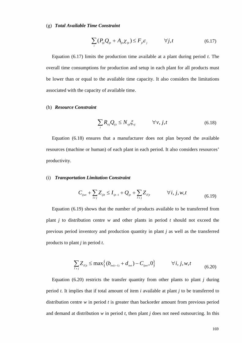
(g) Total Available Time Constraint
( ) ,ijt ijt ijt ijt jt ji
P Q A F j tχ ε+ ≤ ∀∑ (6.17)
Equation (6.17) limits the production time available at a plant during period t. The
overall time consumptions for production and setup in each plant for all products must
be lower than or equal to the available time capacity. It also considers the limitations
associated with the capacity of available time.
(h) Resource Constraint
, ,vij ij t vjt vji
R Q N v j tξ≤ ∀∑ (6.18)
Equation (6.18) ensures that a manufacturer does not plan beyond the available
resources (machine or human) of each plant in each period. It also considers resources’
productivity.
(i) Transportation Limitation Constraint
1 , , ,ijwt ijlt ijt ijt il jtl j l j
C Z I Q Z i j w t′−′≠ ≠
+ ≤ + + ∀∑ ∑ (6.19)
Equation (6.19) shows that the number of products available to be transferred from
plant j to distribution centre w and other plants in period t should not exceed the
previous period inventory and production quantity in plant j as well as the transferred
products to plant j in period t.
( 1)max ( ) ,0 , , ,il jt iw t iwt ijwtl j
Z b d C i j w t′ −′≠
≤ + − ∀∑ (6.20)
Equation (6.20) restricts the transfer quantity from other plants to plant j during
period t. It implies that if total amount of item i available at plant j to be transferred to
distribution centre w in period t is greater than backorder amount from previous period
and demand at distribution w in period t, then plant j does not need outsourcing. In this
169
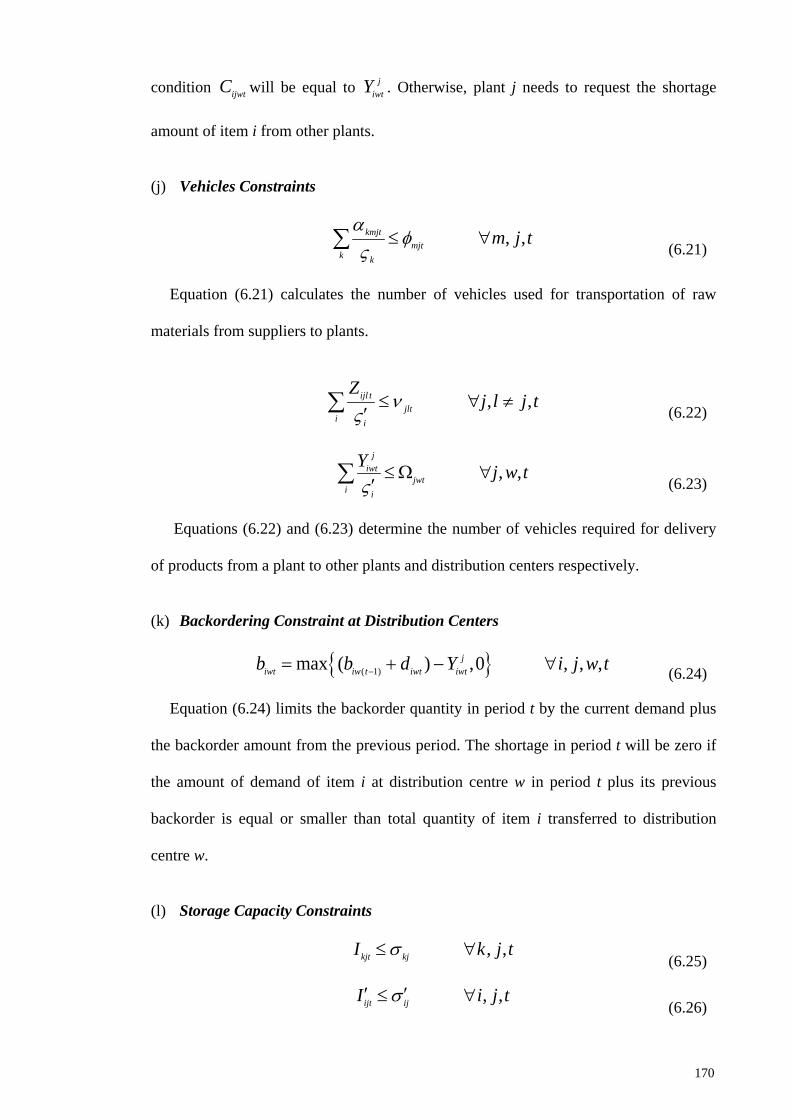
condition ijwtC will be equal to jiwtY . Otherwise, plant j needs to request the shortage
amount of item i from other plants.
(j) Vehicles Constraints
, ,kmjtmjt
k k
m j tα
φς
≤ ∀∑ (6.21)
Equation (6.21) calculates the number of vehicles used for transportation of raw
materials from suppliers to plants.
, ,ijl tjlt
i i
Zj l j tν
ς≤ ∀ ≠
′∑ (6.22)
, ,j
iwtjwt
i i
Y j w tς
≤ Ω ∀′∑
(6.23)
Equations (6.22) and (6.23) determine the number of vehicles required for delivery
of products from a plant to other plants and distribution centers respectively.
(k) Backordering Constraint at Distribution Centers
( 1)max ( ) ,0 , , ,jiwt iw t iwt iwtb b d Y i j w t−= + − ∀ (6.24)
Equation (6.24) limits the backorder quantity in period t by the current demand plus
the backorder amount from the previous period. The shortage in period t will be zero if
the amount of demand of item i at distribution centre w in period t plus its previous
backorder is equal or smaller than total quantity of item i transferred to distribution
centre w.
(l) Storage Capacity Constraints
, ,kjt kjI k j tσ≤ ∀ (6.25)
, ,ijt ijI i j tσ′ ′≤ ∀ (6.26)
170
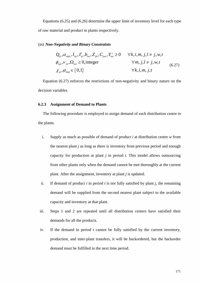
Equations (6.25) and (6.26) determine the upper limit of inventory level for each type
of raw material and product in plants respectively.
(m) Non-Negativity and Binary Constraints
, , , , , , , 0 , , , , , ,, , 0,integer , , , ,
, 0,1 , , , ,
iwt ijlj
ijt kmjt kjt ijt iwt
mjt jlt jwt
ijt kmjt
t ijwtQ I I Y k i m j l j w tm
b Z Cj l j w t
k i m j t
α
φ ν
χ ϕ
′ ≥ ∀ ≠
Ω ≥ ∀ ≠
∈ ∀
(6.27)
Equation (6.27) enforces the restrictions of non-negativity and binary nature on the
decision variables.
6.2.3 Assignment of Demand to Plants
The following procedure is employed to assign demand of each distribution centre to
the plants.
i. Supply as much as possible of demand of product i at distribution centre w from
the nearest plant j as long as there is inventory from previous period and enough
capacity for production at plant j in period t. This model allows outsourcing
from other plants only when the demand cannot be met thoroughly at the current
plant. After the assignment, inventory at plant j is updated.
ii. If demand of product i in period t is not fully satisfied by plant j, the remaining
demand will be supplied from the second nearest plant subject to the available
capacity and inventory at that plant.
iii. Steps 1 and 2 are repeated until all distribution centers have satisfied their
demands for all the products.
iv. If the demand in period t cannot be fully satisfied by the current inventory,
production, and inter-plant transfers, it will be backordered, but the backorder
demand must be fulfilled in the next time period.
171
6.3 Solution Algorithms
The MPCLSP presented in Section 6.2 is a NP-hard problem. To deal with the
intricacy and obtain near-optimal to optimal solutions in a reasonable computation time,
metaheuristic approaches are widely used for which the GA, PSO, ABC, and ICA
approaches are explained in the following subsections. Related codes are presented in
Appendices E to H.
6.3.1 GA Approach
The required steps to solve the proposed model by the GA are explained below.
(a) Parameters
The initial information required to begin a GA includes the number of chromosomes
kept in each generation called population size, ‘Npop’, the probability of operating
crossover, ‘Pc’, the probability of operating mutation, ‘Pm’, and maximum number of
generations, ‘max generation’.
(b) Chromosome Representation
A GA starts with encoding the variables of the problem as finite-length strings or
chromosomes. The chromosomes are considered as strings of the quantities of the
produced items (lot size Q) with N × J × T dimensions where N shows the total number
of products, J indicates total number of plants, and T denotes total number of periods.
The representation of a chromosome is illustrated in Figure 6.2.
Q111 Q112 … Qijt … QNJT-1 QNJT
Figure 6.2: The Structure of a chromosome
172
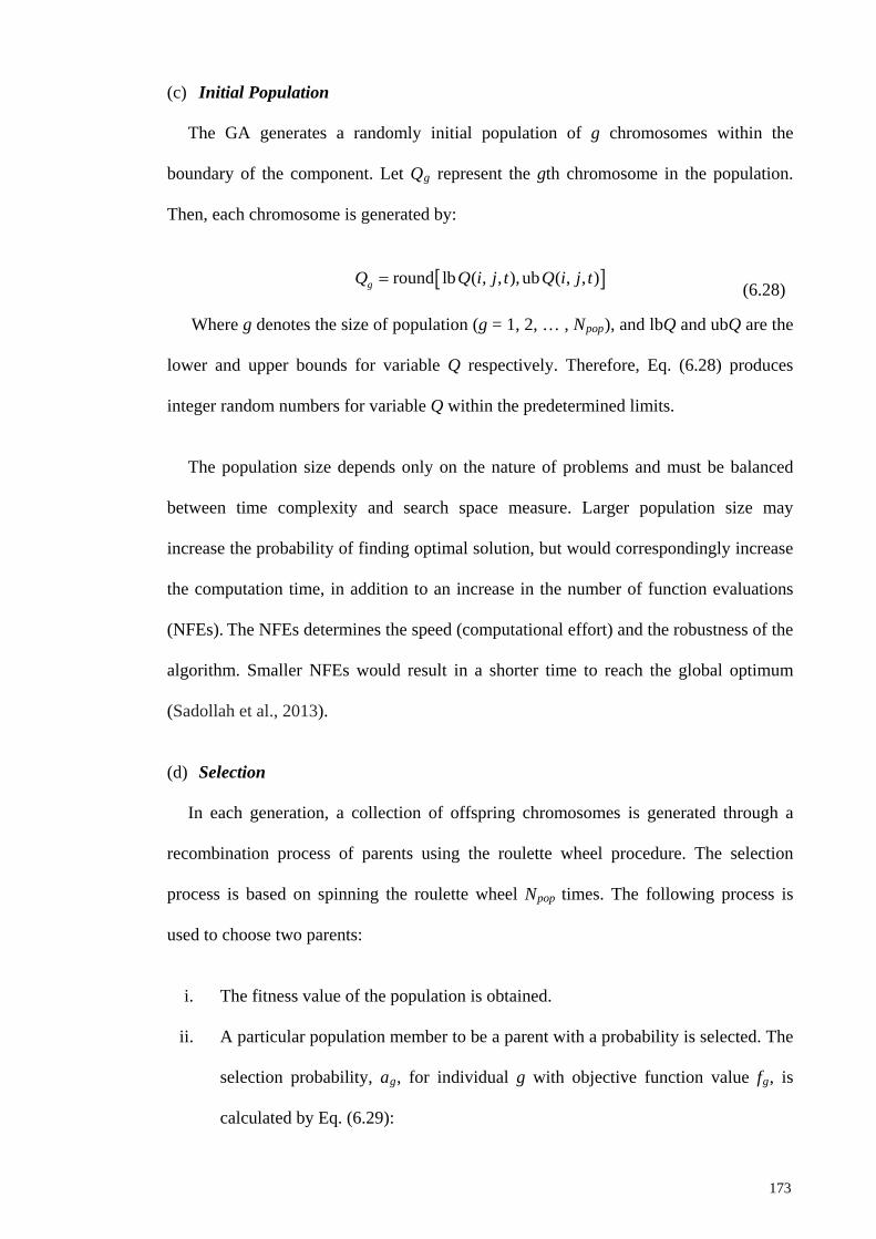
(c) Initial Population
The GA generates a randomly initial population of g chromosomes within the
boundary of the component. Let Qg represent the gth chromosome in the population.
Then, each chromosome is generated by:
[ ]round lb ( , , ), ub ( , , )gQ Q i j t Q i j t= (6.28)
Where g denotes the size of population (g = 1, 2, … , Npop), and lbQ and ubQ are the
lower and upper bounds for variable Q respectively. Therefore, Eq. (6.28) produces
integer random numbers for variable Q within the predetermined limits.
The population size depends only on the nature of problems and must be balanced
between time complexity and search space measure. Larger population size may
increase the probability of finding optimal solution, but would correspondingly increase
the computation time, in addition to an increase in the number of function evaluations
(NFEs). The NFEs determines the speed (computational effort) and the robustness of the
algorithm. Smaller NFEs would result in a shorter time to reach the global optimum
(Sadollah et al., 2013).
(d) Selection
In each generation, a collection of offspring chromosomes is generated through a
recombination process of parents using the roulette wheel procedure. The selection
process is based on spinning the roulette wheel Npop times. The following process is
used to choose two parents:
i. The fitness value of the population is obtained.
ii. A particular population member to be a parent with a probability is selected. The
selection probability, ag, for individual g with objective function value fg, is
calculated by Eq. (6.29):
173
1
gg Npop
gg
fa
f=
=
∑
(6.29)
iii. Cumulative normalized fitness value for each chromosome is then calculated.
iv. A real random number r in range [0, 1] is generated.
v. Two chromosomes are selected whose cumulative probabilities are greater than
r.
Although all individuals in the population have a chance of being selected to
reproduce the next generation, those with higher fitness value are more likely to be
selected for the mating pool.
(e) Crossover
In a crossover process, it is essential to mate pairs of chromosomes to produce
offspring. This is carried out by a random selection of a pair of chromosomes from the
generation with probability Pc. The number of chromosomes for carrying out the
crossover operator is obtained by Eq. (6.30):
crossover pop cN N P= × (6.30)
In this study, the arithmetic crossover operator that linearly combines the parent
chromosome vector is used to produce offspring based on Eqs. (6.31) and (6.32).
(1) (1) (2)(1 )offspring y parent y parent= × + − × (6.31)
(2) (2) (1)(1 )offspring y parent y parent= × + − × (6.32)
Where y is a random vector in range [0, 1], and has a dimension equal to the size of
the selected part (say the first part) of the chosen parent. Because variable Q is integer,
the amounts of produced offsprings are rounded. The crossover process will be repeated
Ncrossover/2 times.
174
(f) Mutation
The mutation operator injects diversity in the population of solutions by perturbing
some of them with probability Pm. The solution spaces that are not discovered by the
crossover operator are found using the mutation operator.
The expected number of chromosomes which undergoes the mutation operation is
obtained using Eq. (6.33):
mutation pop mN N P= × (6.33)
The steps involved in the mutation operation are as follow:
i. An integer random number in range [1, Npop] is generated in order to select a
chromosome (Qg). The total numbers of elements selected for mutation are
n .Q N J T= × ×
ii. Two integer random numbers r1 and r2 are produced in order to select the
elements of the chromosome for mutation. The considered range for r1 is [1, nQ-
1] and r2 is [r1+1, nQ].
iii. The value of selected elements of chromosome Qg is changed using Eq. (6.34):
( ) ( ) ( )1 2 1 2 1 2: : distance :g g gQ r r Q r r Q r r′ = + (6.34)
The distance is the amount an element can be changed as shown in Eq. (6.35):
( )distance 0.1 ub lbg g gQ r Q Q= × × − (6.35)
Where r is a random number generated from the continuous uniform distribution
within the range of [-1, 1]. The size of generated random numbers is to be equal to the
upper bound Qg. Equation (6.35) causes the value of chosen elements exchange with
uniform values randomly selected between the upper and lower range. The result
obtained by Eq. (6.34) is rounded to attain an integer value.
175
However, there is a possibility that the calculated value by Eq. (6.34) exceeds the
upper and lower bounds of Qg. Therefore:
if ub then ub
if lb then lb g g g g
g g g g
Q Q Q QQ Q Q Q
′ ′> = ′ ′< =
(6.36)
In this study, various combinations of the crossover and mutation rates in the range
[0.1, 1] are examined. The computational results show that as Pc and Pm increases, the
total cost will decrease.
(g) Evaluation and Constraint Handling
As the chromosomes are produced, a fitness value is assigned to chromosomes of
each generation for their evaluation. This evaluation is achieved by the objective
function given in Eq. (6.7) which measures the fitness of each individual in the
population.
As shown in subsection 6.2.2, the proposed model contains various constraints,
which may lead to the production of infeasible chromosomes. In order to deal with
infeasibility, a penalty value is assigned to chromosomes that are not feasible. It can be
attained by adding a specific amount to the objective function value according to the
amount of constraints’ violations obtained in a solution.
When a chromosome is feasible, its penalty is set to zero, whereas in case of
infeasibility, the coefficient is selected sufficiently large. Therefore, the fitness function
for a chromosome will be equal to the sum of the objective function value and penalties
as shown in Eq. (6.37), where s represents a solution, and f(s) is the objective function
value for solution s. The penalty policy is employed for all metaheuristic algorithms
utilized in this research.
176
( ); if is feasible
( )( ) Penalty( ); otherwise
f s sfitness s
f s s
= +
(6.37)
(h) New Population
The fitness function values of all chromosomes are evaluated in this stage. The
chromosomes with higher fitness scores are then selected to generate a new population.
Note that the number of chosen chromosomes must be equal to Npop.
(i) Termination
The selection and reproduction of parents will be continued until the algorithm
reaches a stopping criterion. The procedure can be ended after a predetermined number
of generations, or when no substantial improvement over a successive generation is
achieved.
6.3.2 PSO Algorithm
In any iteration of PSO, the velocity and position of particles are updated according
to Eqs. (6.38) and (6.39):
( ) ( )( 1)1 1 2 2
e e e eg g g g g gV V c y best c y globalω ψ ψ+ = + − + −
(6.38)
( 1) ( 1)e e eg g gVψ ψ+ += +
(6.39)
Where g = 1, 2,…, Nswarm and e denotes the iteration (e = 1, 2, …, max iteration). Vg
is the velocity of gth particle.ω is the inertia weight that controls the impact of the
previous velocity of the particle on its current velocity, which plays an important role in
balancing global and local search ability of the PSO. Applying a large inertia weight at
the start of the algorithm and making it decay to a small value through the PSO
execution makes the algorithm search globally at the beginning of the search, and search
locally at the end of the execution (Coelho & Sierakowski, 2008). The inertia weight is
177
updated in each iteration by ( 1) (1 )e eω ω β+ = × − where in this study β is considered
0.01.
c1 is the cognitive parameter, and c2 is the social parameter; y1 and y2 are random
numbers within the range [0, 1], which should be the same size as Vg; bestg is the best
searching experience so far by particle g; gψ is the current position of particle g; and
globalg is the position in parameter space of the best fitness returned for the entire
swarm. The search procedure of the PSO is summarized as follows:
i. Generate an initial population of g particles (solutions) with random positions
and velocities within the boundary of the component according to Eq. (6.28),
where g denotes the size of swarm.
ii. Evaluate the fitness value of each particle in the swarm.
iii. Compare each particle’s fitness with the current particle’s own best. If current
value is better than own best, own best value will be set to the current value, and
the own best location to the current location.
iv. Compare the fitness value with the population’s overall previous best. If the
current value is better than global best, then global best will be set to the current
particle’s array index and value.
v. Update the velocity of each particle g using Eq. (6.38), and the position of
particle g using Eq. (6.39). The values obtained by Eq. (6.38) for the velocity is
rounded to the nearest integer amount. If the value obtained by Eq. (6.39)
exceeds upper and lower bounds of the particle, Eq. (6.36) is used to set the
value to its boundaries.
vi. Terminate the procedure if the termination criterion is satisfied, otherwise go to
step (ii).
178
6.3.3 ABC Algorithm
The main steps of the ABC algorithm are as follow.
(a) Initialization of the Parameters
The main parameters of the ABC algorithm are the total number of bees (NB),
number of food sources (NS) which is equal to the number of the employed bees or
onlooker bees, number of trials after which a food source is supposed to be discarded
(limit), and maximum number of cycles of the search process (max cycle). NS is
considered equal to NB/2.
(b) Initialization of the Population
The ABC algorithm generates a randomly initial population of g solutions (g = 1, 2,
... , NS). Each solution is generated using Eq. (6.28). Their fitness is then evaluated, and
the best fitness is considered as global food source. After initialization, the population
of the food sources (solutions) is subjected to repeat cycles of the search processes of
the employed, onlooker and scout bees.
(c) Employed Bee Phase
For every food source position, only one employed bee is allocated denoting that the
number of food source positions around the hive is equal to the number of employed
bees (Eb). An employed bee makes a modification on the position of the food source in
its memory and finds a neighboring food source, and then evaluates its nectar amount
(fitness) of the associated food source.
In order to determine a neighboring food source position to the previous one in
memory, the algorithm changes some randomly selected parameter and keeps the
remaining parameters unchanged. To select a neighborhood an integer random number
in the range [1, NS] is generated. Within the neighbourhood of every food source site
179
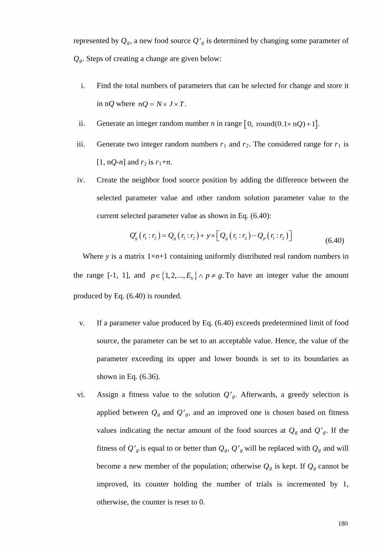
represented by Qg, a new food source Q’g is determined by changing some parameter of
Qg. Steps of creating a change are given below:
i. Find the total numbers of parameters that can be selected for change and store it
in nQ where n .Q N J T= × ×
ii. Generate an integer random number n in range [ ]0, round 0.1 1 .n( )Q× +
iii. Generate two integer random numbers r1 and r2. The considered range for r1 is
[1, nQ-n] and r2 is r1+n.
iv. Create the neighbor food source position by adding the difference between the
selected parameter value and other random solution parameter value to the
current selected parameter value as shown in Eq. (6.40):
( ) ( ) ( ) ( )1 2 1 2 1 2 1 2: : : :g g g pQ r r Q r r y Q r r Q r r′ = + × − (6.40)
Where y is a matrix 1×n+1 containing uniformly distributed real random numbers in
the range [-1, 1], and 1,2,..., .bp E p g∈ ∧ ≠ To have an integer value the amount
produced by Eq. (6.40) is rounded.
v. If a parameter value produced by Eq. (6.40) exceeds predetermined limit of food
source, the parameter can be set to an acceptable value. Hence, the value of the
parameter exceeding its upper and lower bounds is set to its boundaries as
shown in Eq. (6.36).
vi. Assign a fitness value to the solution Q’g. Afterwards, a greedy selection is
applied between Qg and Q’g, and an improved one is chosen based on fitness
values indicating the nectar amount of the food sources at Qg and Q’g. If the
fitness of Q’g is equal to or better than Qg, Q’g will be replaced with Qg and will
become a new member of the population; otherwise Qg is kept. If Qg cannot be
improved, its counter holding the number of trials is incremented by 1,
otherwise, the counter is reset to 0.
180
(d) Onlooker Bee Phase
After all employed bees complete their searches, they share their information related
to the nectar amounts and the positions of their sources with the onlooker bees on the
dance area. An onlooker bee evaluates the nectar information taken from all the
employed bees and chooses a food source Qg depending on its probability value ag
calculated by Eq. (6.41):
1
gg NS
gg
fa
f=
=
∑
(6.41)
Where fg is the fitness value of the gth food source. Obviously, the higher the fg, the
more probability that the gth food source is selected.
To select a food source a real random number within the range [0, 1] is generated. If
the cumulative probability ag associated with that source is greater than this random
number then the onlooker bee produces a modification on the position of this food
source site using Eq. (6.40).
To select a neighborhood an integer random number in range [1, NS] is generated.
After the new food source is evaluated, greedy selection is applied and the onlooker bee
either memorizes the new position by forgetting the old one or keeps the old one. If
solution Qg cannot be improved, its counter holding trials is incremented by 1,
otherwise, the counter is reset to 0. This process is repeated until all onlookers are
distributed onto food source sites.
(e) Scout Bee Phase
In a cycle, a food source that cannot be improved through limit cycle is abandoned.
In order to select a food source to be abandoned, a control parameter called limit is used.
If a solution representing a food source is not improved by a predetermined number of
181
trials, then that food source is abandoned by its employed bee and the employed bee is
converted to a scout. The number of trials for releasing a food source is equal to the
value of limit. Then a scout bee is employed to search new food source randomly using
Eq. (6.28) to replace the abandoned one.
It is supposed that only one source can be exhausted in each cycle, and only one
employed bee can be a scout. If more than one counter exceeds the limit value, one of
the maximum ones might be chosen programmatically. After every cycle, the best
solution is memorized.
The process is repeated until a termination criterion is reached which can be reaching
the maximum number of iterations, or when the algorithm does not seem to converge in
its initial phase.
6.3.4 ICA Approach
The ICA approach is a population based evolutionary algorithm, which has been
used extensively to solve various kinds of combinatorial optimization problems. This
method is based on socio-political process of imperialistic competition. The main steps
of the ICA are described below.
(a) The Initialization Mechanism
Similar to other optimization methods, the ICA first creates the initial population.
Each individual of the population is named a ‘country’. The word ‘country’ corresponds
to the ‘chromosome’ in the GA terminology. This array is shown in Eq. (6.42).
1 2country [ , , , ]NL L L= … (6.42)
Where Ls are the variables to be optimized. The power of a country is inversely
proportional to its fitness function value which is obtained by evaluation of cost
function f at variables as shown in Eq. (6.43).
182
1 2cost (country) ])([ , , , Nf f L L L= = … (6.43)
Equation (6.28) is used to create the initial population of size Ncountry and Eq. (6.7) is
used to evaluate the fitness of variable. Based on cost values, a certain number of
countries that have the lowest costs are selected as imperialist (Nimp) and the rest,
known as colonies (Ncolony = Ncountry – Nimp), are divided among these imperialists. Each
imperialist and its allocated colonies form an empire.
(b) Assimilation of Colonies
The imperialist countries would try to absorb their colonies toward themselves. For
this purpose the assimilation policy is considered in the ICA. Based on this concept
each colony moves toward its imperialist by X units as shown in Eq. (6.44).
1 e eg gQ Q X+ = +
(6.44)
Where egQ and 1e
gQ + are the current and new position of gth colony of each empire
respectively, e is the number of iteration (knows as decade in the ICA), and X is:
=X y Dβ × × (6.45)
Where D is the distance between the initial position of colony and its imperialist (D =
imp. egQ - colony. e
gQ ). The position of the colony after movement is defined by the
random parameter y in range [0, 1], which must have the dimension equal to the size of
D. Parameter 1β > causes the colony to get closer to its imperialist from different
directions. 2β = results in good convergence of countries to the global minimum in
most of the implementations. If the value of 1egQ + exceeds its predetermined limit, it
must be set to its upper and lower bounds as shown in Eq. (6.36). Then, fitness of 1egQ +
will be evaluated.
183
(c) Revolution
Revolution is a fundamental change in power or organizational structures that takes
place in a relatively short period of time. The revolution increases the exploration of the
algorithm and avoids the early convergence of countries to local minimum with a
revolution rate. A very high value of revolution rate reduces the exploitation power of
algorithm as well as the convergence rate (Nazari-Shirkouhi et al., 2010). This
mechanism is similar to mutation process in the GA for creating diversification in
solutions.
Mutation increases the variety in the population, so this operator is used for creating
a revolution in variables same as the GA. For this purpose random number r in range [0,
1] is generated. If r is smaller than revolution rate (θ ), a change will be applied on the
selected colony of the particular imperialist. Steps of creating a change are as follow:
i. Find the total numbers of elements of the colony that can be chosen for change
and store it in nQ where n .Q N J T= × ×
ii. Generate an integer random number n in range [ ]0, round 0.01 1 .n( )Q× +
iii. Generate two integer random numbers r1 and r2. The considered range for r1 is
[1, nQ-n] and r2 is r1+n.
iv. Create the change using Eq. (6.46):
( ) ( ) ( ) ( )11 2 1 2 1 2 1 2: lb : ub : lb :e e e e
g g g gQ r r Q r r y Q r r Q r r+ = −+ × (6.46)
Where y is a matrix 1×n+1 containing real random numbers in the range [0, 1], and
lb egQ and ub e
gQ are the lower and upper bounds of gth colony in decade e. Values
obtained by Eq. (6.46) are rounded to the nearest integers. Then, fitness of new colony
is evaluated.
184
(d) Exchange the Colony with Imperialist
After moving toward the imperialist, a colony may reach a position with lower cost
than its imperialist. In this case, the colony will become the imperialist in the current
empire and vice versa. In the next decades, colonies in the empire will move towards
the new imperialist.
(e) Total Power of an Empire
Based on total power of empires, an imperialistic competition takes place between
empires. Total power of an empire is mainly affected by the power of its imperialist and
slightly by its colonies. Hence, total power of an empire is calculated by Eq. (6.47):
= (imp )+ mean[ (colony of empire )]g g gTf f fγ × (6.47)
Where Tfg is the total cost of the gth empire and γ is a positive number in the range
of [0, 1]. The small value of γ makes the total power of the empire to be determined by
almost only its imperialist and increasing it will enhance the role of the colonies in
determining the total power of an empire.
(f) Imperialistic Competition
Every empire tries to take over the colonies of other empires. The imperialistic
competition gradually causes reduction in power of weaker empires and growth in
power of powerful ones. The imperialistic competition is modeled by selecting the
weakest colonies of the weakest empire in every iteration and making a competition
among all empires to take over this colony. The likelihood of possession of the colony
for each empire is proportionate to its total power.
The normalized total cost of an empire can be obtained by Eq. (6.48):
max( ) -g g gNTf Tf Tf ε′= + (6.48)
185
ε is a small number to avoid the value of NTfg to become exactly zero. NTfg and Tfg
are the normalized total cost and total cost of gth empire respectively. Having the
normalized total cost, the possession probability of gth empire is obtained by Eq. (6.49):
1
imp
gg N
gg
NTfa
NTf ′′=
=
∑
(6.49)
Powerful empires have higher chance of possessing the colony. To distribute the
mentioned colony among empires vector c is formed as follows:
1 2, ,..., Nimpc c c c =
(6.50)
Then, vector h with uniformly distributed random numbers in range [0, 1] is created
which has the same size as c:
1 2, ,..., Nimph h h h =
(6.51)
Vector z is formed by subtracting h from c:
1 2, ,..., Nimpz c h z z z = − =
(6.52)
Referring to vector z, the mentioned colony is handed to an empire whose
corresponding index in z is maximum (Atashpaz-Gargari & Lucas, 2007).
(g) Elimination of Powerless Empires
Powerless empires will collapse in the imperialistic competition and their colonies
will be divided among other empires. It is assumed that an empire would collapse and
be removed when it loses all of its colonies. This process will be continued and causes
the countries to converge to the global minimum of the cost function. At the end, all the
empires will collapse except the most powerful one, and all the colonies would be
handled by this unique empire. At this stage, the imperialist and colonies would have
the same position and power (Atashpaz-Gargari & Lucas, 2007).
186
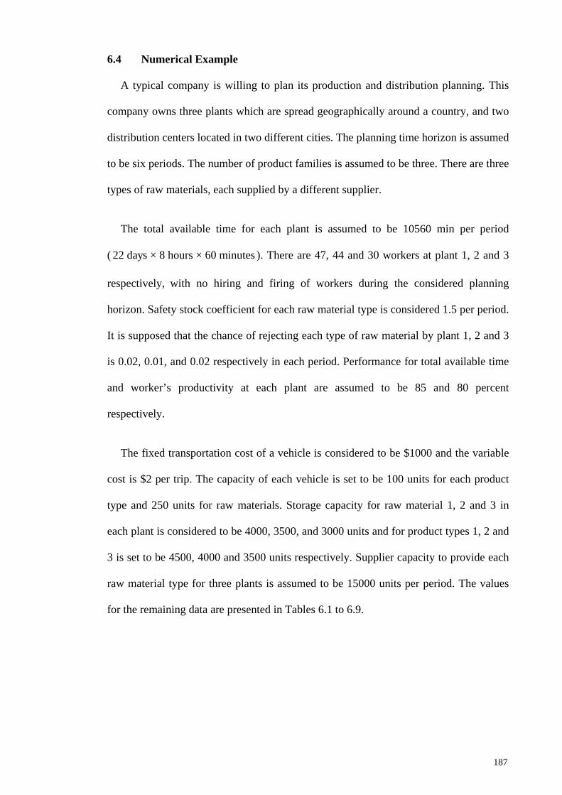
6.4 Numerical Example
A typical company is willing to plan its production and distribution planning. This
company owns three plants which are spread geographically around a country, and two
distribution centers located in two different cities. The planning time horizon is assumed
to be six periods. The number of product families is assumed to be three. There are three
types of raw materials, each supplied by a different supplier.
The total available time for each plant is assumed to be 10560 min per period
( 22 days × 8 hours × 60 minutes ). There are 47, 44 and 30 workers at plant 1, 2 and 3
respectively, with no hiring and firing of workers during the considered planning
horizon. Safety stock coefficient for each raw material type is considered 1.5 per period.
It is supposed that the chance of rejecting each type of raw material by plant 1, 2 and 3
is 0.02, 0.01, and 0.02 respectively in each period. Performance for total available time
and worker’s productivity at each plant are assumed to be 85 and 80 percent
respectively.
The fixed transportation cost of a vehicle is considered to be $1000 and the variable
cost is $2 per trip. The capacity of each vehicle is set to be 100 units for each product
type and 250 units for raw materials. Storage capacity for raw material 1, 2 and 3 in
each plant is considered to be 4000, 3500, and 3000 units and for product types 1, 2 and
3 is set to be 4500, 4000 and 3500 units respectively. Supplier capacity to provide each
raw material type for three plants is assumed to be 15000 units per period. The values
for the remaining data are presented in Tables 6.1 to 6.9.
187
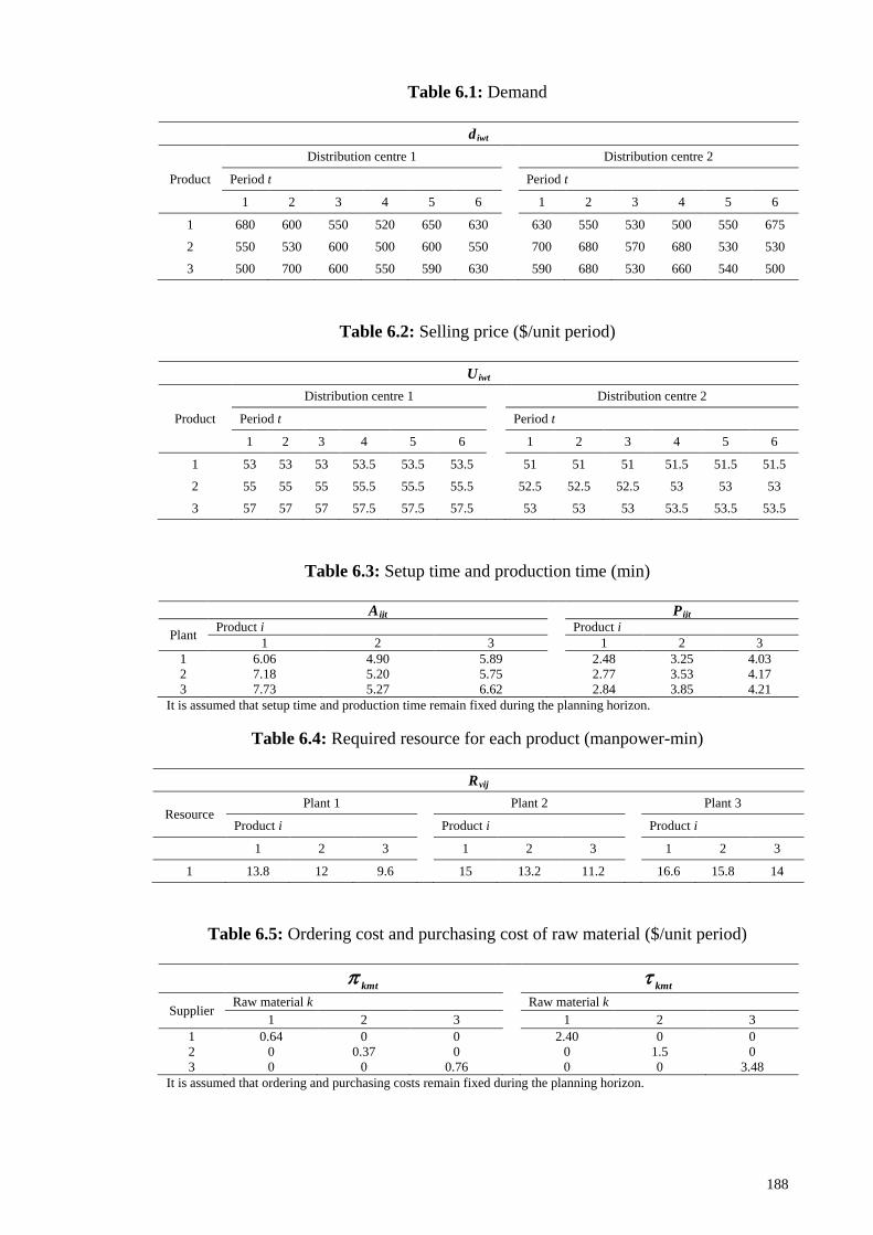
Table 6.1: Demand
diwt
Product
Distribution centre 1 Distribution centre 2
Period t Period t
1 2 3 4 5 6 1 2 3 4 5 6
1 680 600 550 520 650 630 630 550 530 500 550 675
2 550 530 600 500 600 550 700 680 570 680 530 530
3 500 700 600 550 590 630 590 680 530 660 540 500
Table 6.2: Selling price ($/unit period)
Uiwt
Product
Distribution centre 1 Distribution centre 2
Period t Period t
1 2 3 4 5 6 1 2 3 4 5 6
1 53 53 53 53.5 53.5 53.5 51 51 51 51.5 51.5 51.5
2 55 55 55 55.5 55.5 55.5 52.5 52.5 52.5 53 53 53
3 57 57 57 57.5 57.5 57.5 53 53 53 53.5 53.5 53.5
Table 6.3: Setup time and production time (min)
Aijt Pijt
Plant Product i Product i 1 2 3 1 2 3
1 6.06 4.90 5.89 2.48 3.25 4.03 2 7.18 5.20 5.75 2.77 3.53 4.17 3 7.73 5.27 6.62 2.84 3.85 4.21
It is assumed that setup time and production time remain fixed during the planning horizon.
Table 6.4: Required resource for each product (manpower-min)
Rvij
Resource Plant 1 Plant 2 Plant 3
Product i Product i Product i
1 2 3 1 2 3 1 2 3
1 13.8 12 9.6 15 13.2 11.2 16.6 15.8 14
Table 6.5: Ordering cost and purchasing cost of raw material ($/unit period)
kmtπ τ kmt
Supplier Raw material k
Raw material k
1 2 3 1 2 3 1 0.64 0 0 2.40 0 0 2 0 0.37 0 0 1.5 0 3 0 0 0.76 0 0 3.48
It is assumed that ordering and purchasing costs remain fixed during the planning horizon.
188
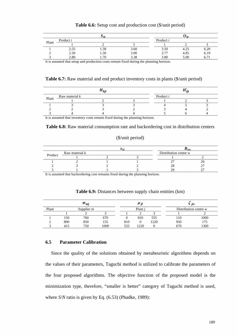
Table 6.6: Setup cost and production cost ($/unit period)
Sijt Oijt Plant Product i Product i
1 2 3 1 2 3 1 2.55 1.58 3.60 3.50 4.25 6.20 2 2.50 1.50 3.00 3.77 4.85 6.19 3 2.80 1.70 3.38 3.80 5.00 6.71
It is assumed that setup and production costs remain fixed during the planning horizon.
Table 6.7: Raw material and end product inventory costs in plants ($/unit period)
kjtH ijtH ′
Plant Raw material k Product i 1 2 3 1 2 3
1 3 3 3 4 5 3 2 2 3 2 3 4 2 3 4 4 4 5 6 4
It is assumed that inventory costs remain fixed during the planning horizon.
Table 6.8: Raw material consumption rate and backordering cost in distribution centers
($/unit period)
xki Biwt
Product Raw material k Distribution centre w 1 2 3 1 2
1 2 1 1 27 26 2 3 2 2 28 27 3 1 1 3 29 27
It is assumed that backordering cost remains fixed during the planning horizon.
Table 6.9: Distances between supply chain entities (km)
6.5 Parameter Calibration
Since the quality of the solutions obtained by metaheuristic algorithms depends on
the values of their parameters, Taguchi method is utilized to calibrate the parameters of
the four proposed algorithms. The objective function of the proposed model is the
minimization type, therefore, “smaller is better” category of Taguchi method is used,
where S/N ratio is given by Eq. (6.53) (Phadke, 1989):
mjϖ jlµ jwζ
Plant Supplier m Plant j Distribution centre w 1 2 3 1 2 3 1 2
1 150 760 670 0 810 555 110 1000 2 800 850 155 810 0 1220 950 175 3 415 750 1000 555 1220 0 670 1300
189
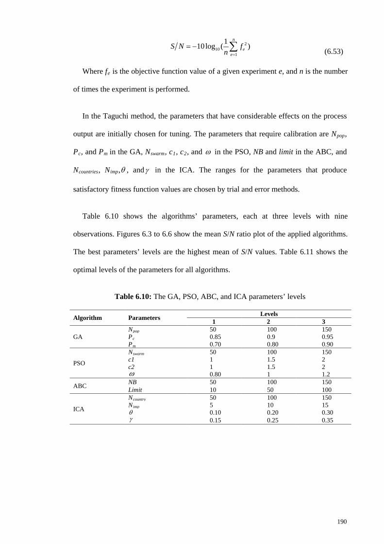
210
1
110log ( )n
ee
S N fn =
= − ∑ (6.53)
Where fe is the objective function value of a given experiment e, and n is the number
of times the experiment is performed.
In the Taguchi method, the parameters that have considerable effects on the process
output are initially chosen for tuning. The parameters that require calibration are Npop,
Pc, and Pm in the GA, Nswarm, c1, c2, and ω in the PSO, NB and limit in the ABC, and
Ncountries, Nimp,θ , andγ in the ICA. The ranges for the parameters that produce
satisfactory fitness function values are chosen by trial and error methods.
Table 6.10 shows the algorithms’ parameters, each at three levels with nine
observations. Figures 6.3 to 6.6 show the mean S/N ratio plot of the applied algorithms.
The best parameters’ levels are the highest mean of S/N values. Table 6.11 shows the
optimal levels of the parameters for all algorithms.
Table 6.10: The GA, PSO, ABC, and ICA parameters’ levels
Algorithm Parameters Levels 1 2 3
GA Npop 50 100 150 Pc 0.85 0.9 0.95 Pm 0.70 0.80 0.90
PSO
Nswarm 50 100 150 c1 1 1.5 2 c2 1 1.5 2 ω 0.80 1 1.2
ABC NB 50 100 150 Limit 10 50 100
ICA
Ncountry 50 100 150 Nimp 5 10 15 θ 0.10 0.20 0.30 γ 0.15 0.25 0.35
190
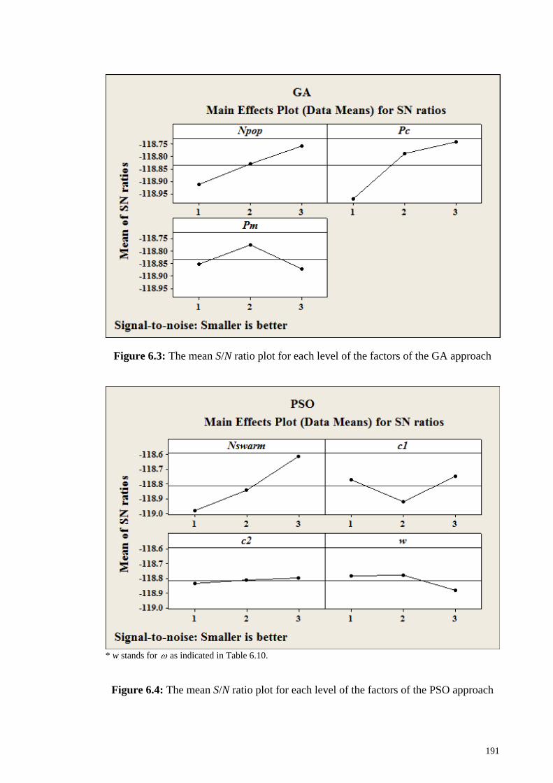
Figure 6.3: The mean S/N ratio plot for each level of the factors of the GA approach
* w stands for ω as indicated in Table 6.10.
Figure 6.4: The mean S/N ratio plot for each level of the factors of the PSO approach
191
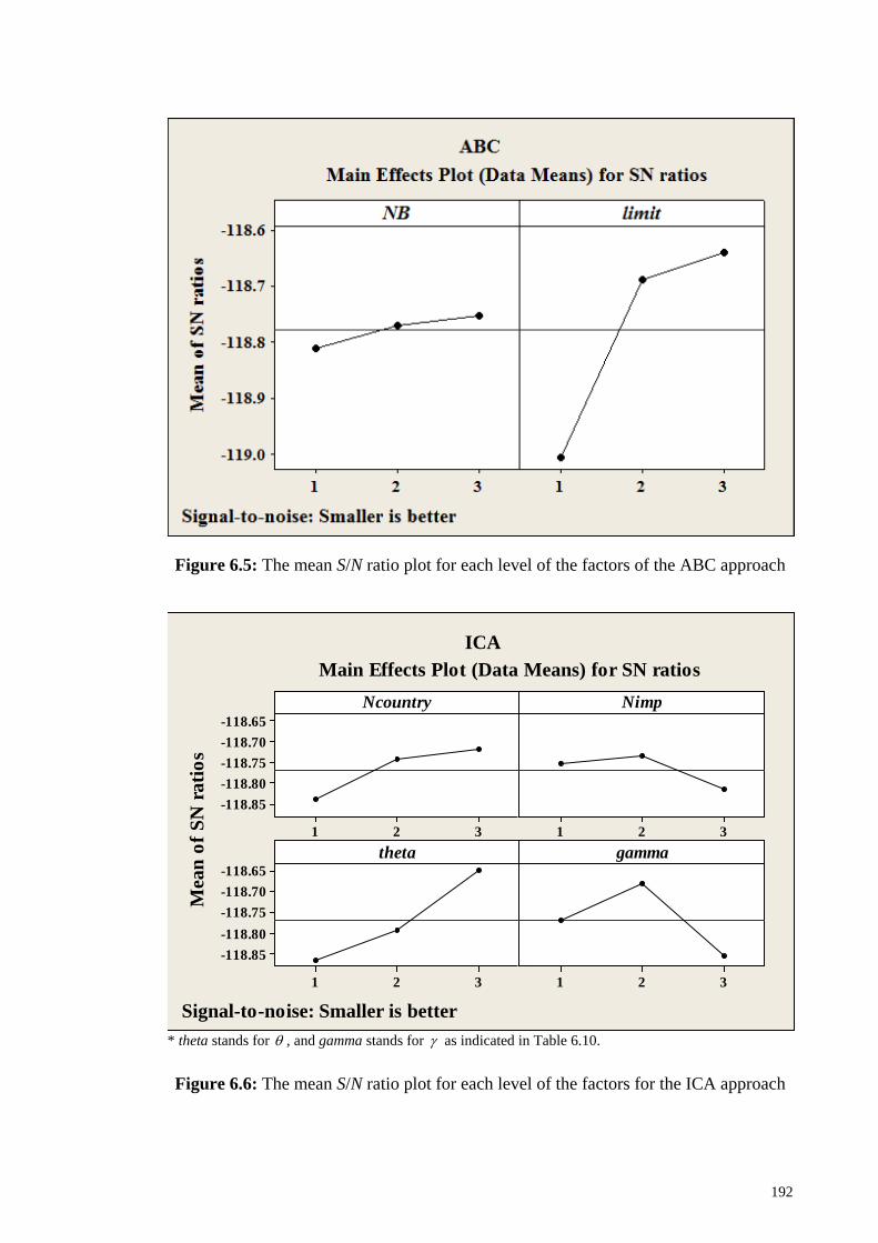
Figure 6.5: The mean S/N ratio plot for each level of the factors of the ABC approach
321
-118.65-118.70-118.75-118.80-118.85
321
321
-118.65-118.70-118.75-118.80-118.85
321
Ncountry
Mea
n of
SN
rat
ios
Nimp
theta gamma
ICAMain Effects Plot (Data Means) for SN ratios
Signal-to-noise: Smaller is better* theta stands for θ , and gamma stands for γ as indicated in Table 6.10.
Figure 6.6: The mean S/N ratio plot for each level of the factors for the ICA approach
192
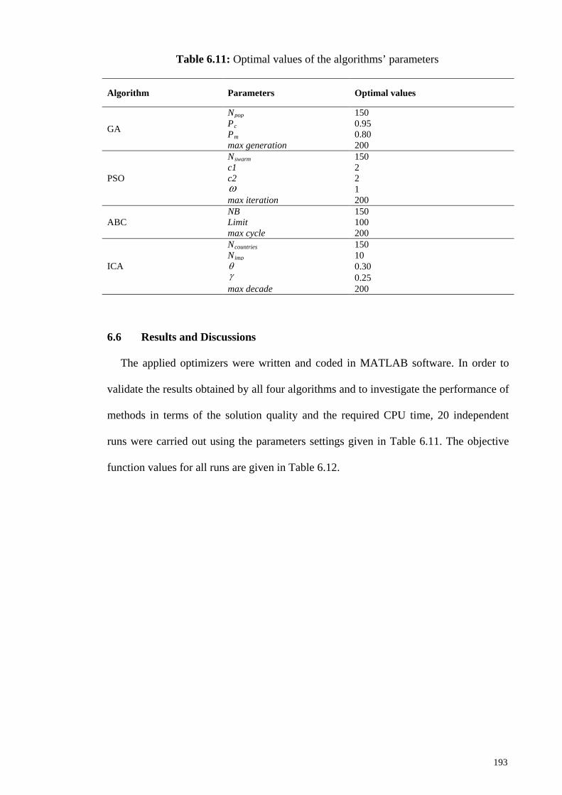
Table 6.11: Optimal values of the algorithms’ parameters
Algorithm Parameters Optimal values
GA
Npop 150 Pc 0.95 Pm 0.80 max generation 200
PSO
Nswarm 150 c1 2 c2 2 ω 1 max iteration 200
ABC NB 150 Limit 100 max cycle 200
ICA
Ncountries 150 Nimp 10 θ 0.30 γ 0.25 max decade 200
6.6 Results and Discussions
The applied optimizers were written and coded in MATLAB software. In order to
validate the results obtained by all four algorithms and to investigate the performance of
methods in terms of the solution quality and the required CPU time, 20 independent
runs were carried out using the parameters settings given in Table 6.11. The objective
function values for all runs are given in Table 6.12.
193
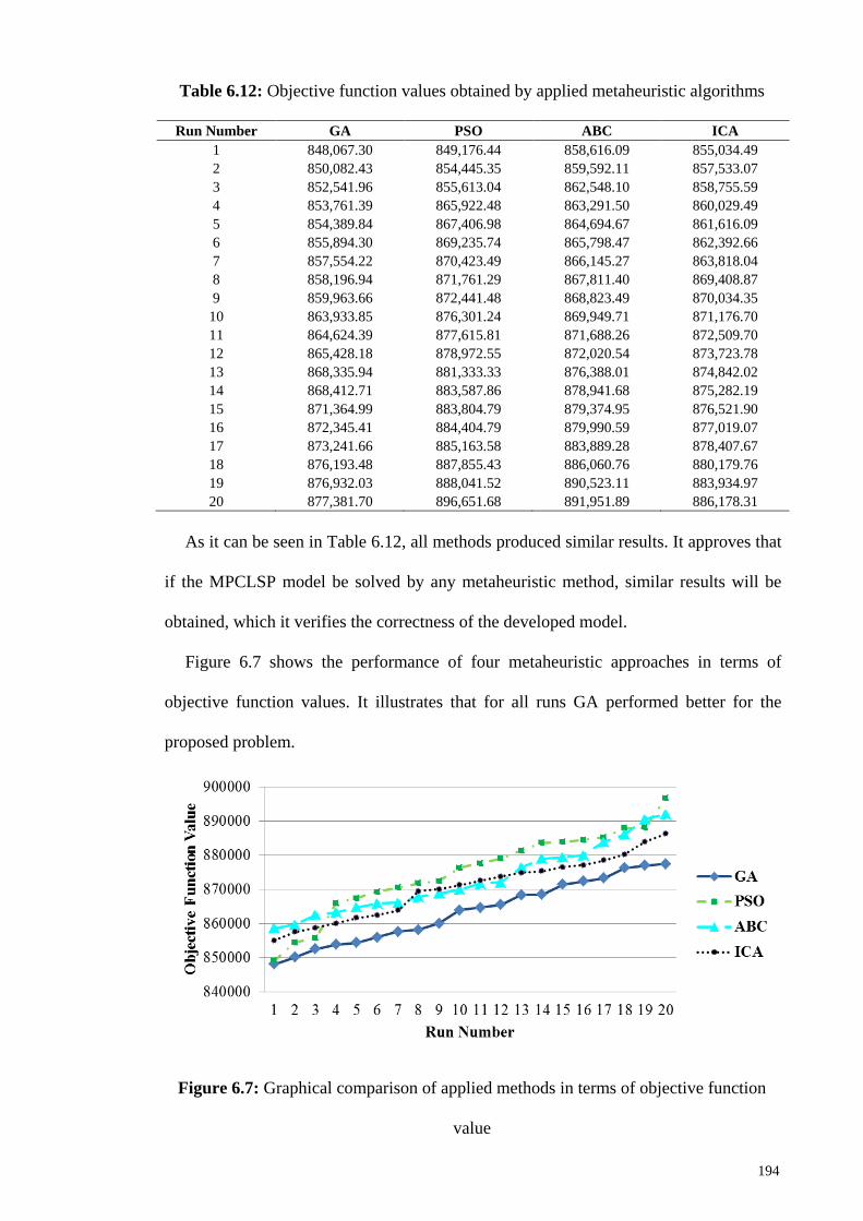
Table 6.12: Objective function values obtained by applied metaheuristic algorithms
Run Number GA PSO ABC ICA 1 848,067.30 849,176.44 858,616.09 855,034.49 2 850,082.43 854,445.35 859,592.11 857,533.07 3 852,541.96 855,613.04 862,548.10 858,755.59 4 853,761.39 865,922.48 863,291.50 860,029.49 5 854,389.84 867,406.98 864,694.67 861,616.09 6 855,894.30 869,235.74 865,798.47 862,392.66 7 857,554.22 870,423.49 866,145.27 863,818.04 8 858,196.94 871,761.29 867,811.40 869,408.87 9 859,963.66 872,441.48 868,823.49 870,034.35
10 863,933.85 876,301.24 869,949.71 871,176.70 11 864,624.39 877,615.81 871,688.26 872,509.70 12 865,428.18 878,972.55 872,020.54 873,723.78 13 868,335.94 881,333.33 876,388.01 874,842.02 14 868,412.71 883,587.86 878,941.68 875,282.19 15 871,364.99 883,804.79 879,374.95 876,521.90 16 872,345.41 884,404.79 879,990.59 877,019.07 17 873,241.66 885,163.58 883,889.28 878,407.67 18 876,193.48 887,855.43 886,060.76 880,179.76 19 876,932.03 888,041.52 890,523.11 883,934.97 20 877,381.70 896,651.68 891,951.89 886,178.31
As it can be seen in Table 6.12, all methods produced similar results. It approves that
if the MPCLSP model be solved by any metaheuristic method, similar results will be
obtained, which it verifies the correctness of the developed model.
Figure 6.7 shows the performance of four metaheuristic approaches in terms of
objective function values. It illustrates that for all runs GA performed better for the
proposed problem.
Figure 6.7: Graphical comparison of applied methods in terms of objective function
value
194
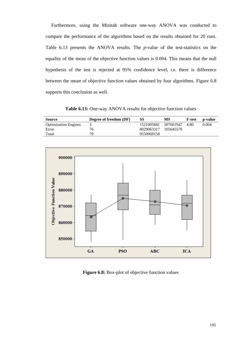
Furthermore, using the Minitab software one-way ANOVA was conducted to
compare the performance of the algorithms based on the results obtained for 20 runs.
Table 6.13 presents the ANOVA results. The p-value of the test-statistics on the
equality of the mean of the objective function values is 0.004. This means that the null
hypothesis of the test is rejected at 95% confidence level, i.e. there is difference
between the mean of objective function values obtained by four algorithms. Figure 6.8
supports this conclusion as well.
Table 6.13: One-way ANOVA results for objective function values
Source Degree of freedom (DF) SS MS F-test p-value Optimization Engines 3 1521005841 507001947 4.80 0.004 Error 76 8029063317 105645570 Total 79 9550069158
Figure 6.8: Box-plot of objective function values
195

The statistical optimization results obtained from four algorithms including the
worst, mean, best solutions, standard deviation (SD), and NFEs are listed in Table 6.14.
Table 6.14: Statistical results obtained from four metaheuristic algorithms
Methods Worst solution Mean solution Best solution SD NFEs GA 877381.70 863432.32 848067.30 9380.23 37616 PSO 896651.68 875007.94 849176.44 12328.95 20550 ABC 891951.89 872904.99 858616.09 10015.37 29779 ICA 886178.31 870419.94 855034.49 9071.00 36643
Based on Table 6.14, the GA is found to be superior to other methods and surpassed
the PSO, ABC, and ICA in terms of function value (accuracy). The GA method has
found the best solution (848067.30) in 37616 function evaluations (143 generations).
Although the PSO offered modest solution quality with a smaller number of function
evaluations (20550), its average cost and SD in 20 experiments are inferior to the other
methods. The performances of the ABC and ICA are almost similar in terms of
objective function value.
The convergence paths of applied methods in terms of best and mean costs for the
best run are plotted in Figures 6.9 to 6.12.
196
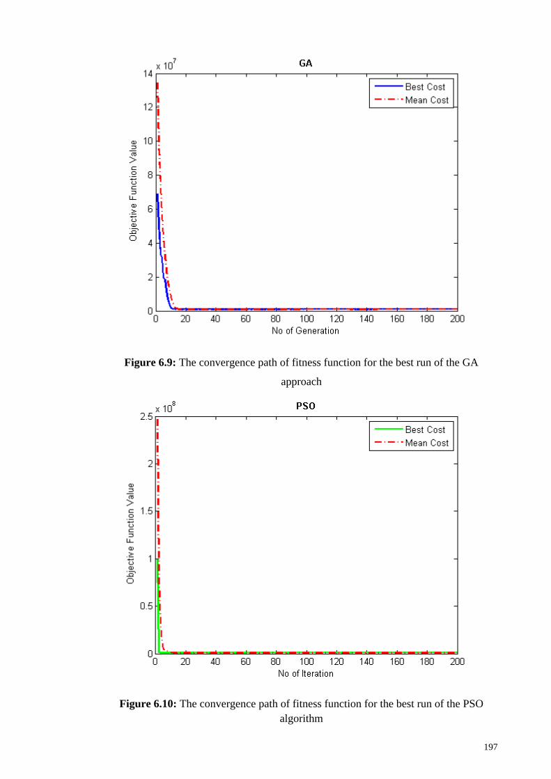
Figure 6.9: The convergence path of fitness function for the best run of the GA
approach
Figure 6.10: The convergence path of fitness function for the best run of the PSO algorithm
197
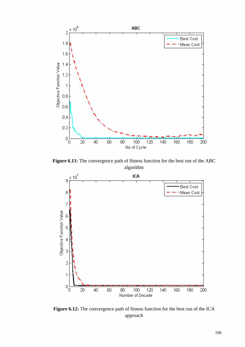
Figure 6.11: The convergence path of fitness function for the best run of the ABC algorithm
Figure 6.12: The convergence path of fitness function for the best run of the ICA approach
198
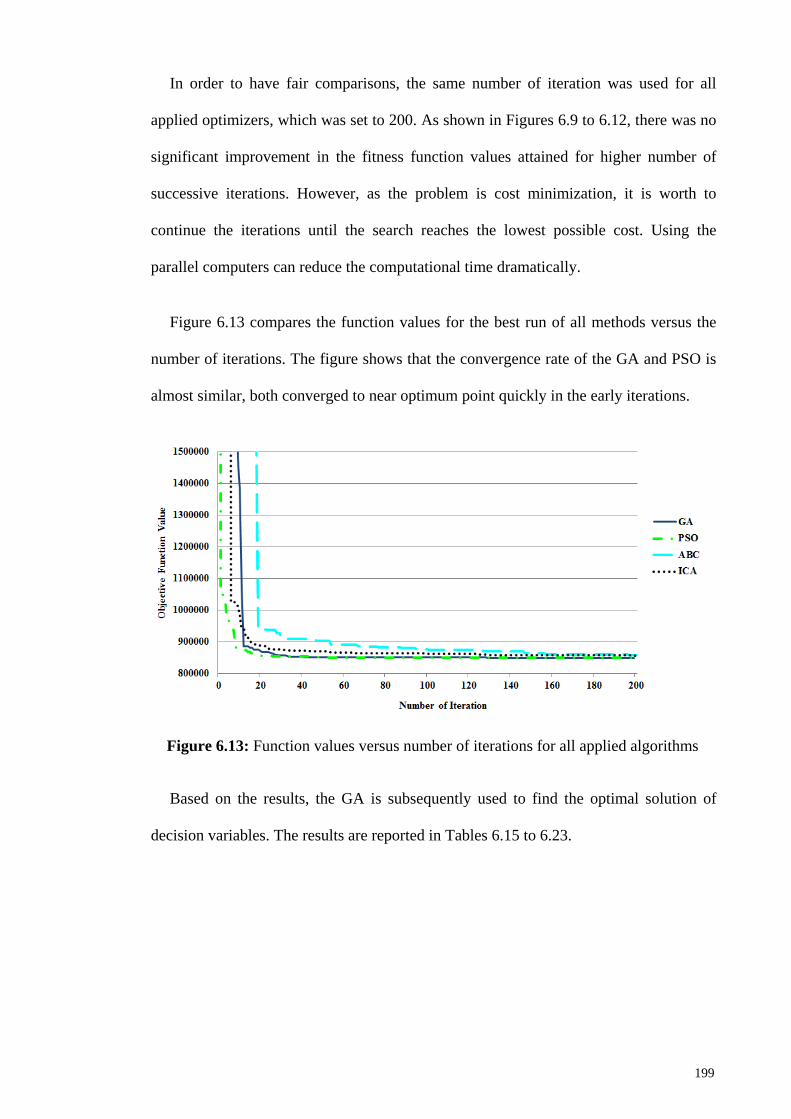
In order to have fair comparisons, the same number of iteration was used for all
applied optimizers, which was set to 200. As shown in Figures 6.9 to 6.12, there was no
significant improvement in the fitness function values attained for higher number of
successive iterations. However, as the problem is cost minimization, it is worth to
continue the iterations until the search reaches the lowest possible cost. Using the
parallel computers can reduce the computational time dramatically.
Figure 6.13 compares the function values for the best run of all methods versus the
number of iterations. The figure shows that the convergence rate of the GA and PSO is
almost similar, both converged to near optimum point quickly in the early iterations.
Figure 6.13: Function values versus number of iterations for all applied algorithms
Based on the results, the GA is subsequently used to find the optimal solution of
decision variables. The results are reported in Tables 6.15 to 6.23.
199
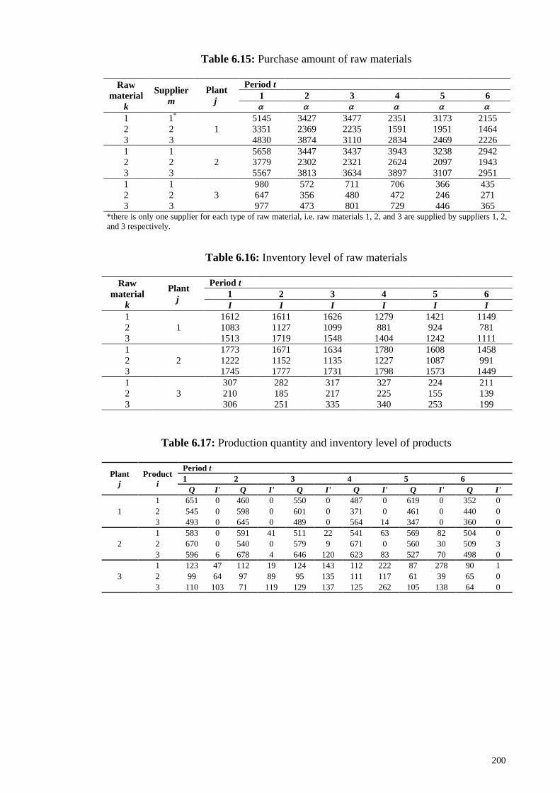
Table 6.15: Purchase amount of raw materials
Raw material
k
Supplier m
Plant j
Period t 1 2 3 4 5 6 α α α α α α
1 1* 1
5145 3427 3477 2351 3173 2155 2 2 3351 2369 2235 1591 1951 1464 3 3 4830 3874 3110 2834 2469 2226 1 1
2 5658 3447 3437 3943 3238 2942
2 2 3779 2302 2321 2624 2097 1943 3 3 5567 3813 3634 3897 3107 2951 1 1
3 980 572 711 706 366 435
2 2 647 356 480 472 246 271 3 3 977 473 801 729 446 365
*there is only one supplier for each type of raw material, i.e. raw materials 1, 2, and 3 are supplied by suppliers 1, 2, and 3 respectively.
Table 6.16: Inventory level of raw materials
Raw material
k
Plant j
Period t 1 2 3 4 5 6 I I I I I I
1 1
1612 1611 1626 1279 1421 1149 2 1083 1127 1099 881 924 781 3 1513 1719 1548 1404 1242 1111 1
2 1773 1671 1634 1780 1608 1458
2 1222 1152 1135 1227 1087 991 3 1745 1777 1731 1798 1573 1449 1
3 307 282 317 327 224 211
2 210 185 217 225 155 139 3 306 251 335 340 253 199
Table 6.17: Production quantity and inventory level of products
Plant j
Product i
Period t 1 2 3 4 5 6
Q I' Q I' Q I' Q I' Q I' Q I'
1 1 651 0 460 0 550 0 487 0 619 0 352 0 2 545 0 598 0 601 0 371 0 461 0 440 0 3 493 0 645 0 489 0 564 14 347 0 360 0
2 1 583 0 591 41 511 22 541 63 569 82 504 0 2 670 0 540 0 579 9 671 0 560 30 509 3 3 596 6 678 4 646 120 623 83 527 70 498 0
3 1 123 47 112 19 124 143 112 222 87 278 90 1 2 99 64 97 89 95 135 111 117 61 39 65 0 3 110 103 71 119 129 137 125 262 105 138 64 0
200
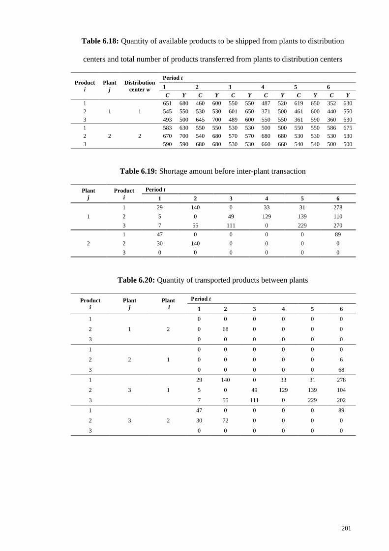
Table 6.18: Quantity of available products to be shipped from plants to distribution
centers and total number of products transferred from plants to distribution centers
Product i
Plant j
Distribution center w
Period t 1 2 3 4 5 6 C Y C Y C Y C Y C Y C Y
1 1 1
651 680 460 600 550 550 487 520 619 650 352 630 2 545 550 530 530 601 650 371 500 461 600 440 550 3 493 500 645 700 489 600 550 550 361 590 360 630 1
2 2 583 630 550 550 530 530 500 500 550 550 586 675
2 670 700 540 680 570 570 680 680 530 530 530 530 3 590 590 680 680 530 530 660 660 540 540 500 500
Table 6.19: Shortage amount before inter-plant transaction
Plant j
Product i
Period t 1 2 3 4 5 6
1 1 29 140 0 33 31 278 2 5 0 49 129 139 110 3 7 55 111 0 229 270
2 1 47 0 0 0 0 89 2 30 140 0 0 0 0 3 0 0 0 0 0 0
Table 6.20: Quantity of transported products between plants
Product i
Plant j
Plant l
Period t
1 2 3 4 5 6
1
1 2
0 0 0 0 0 0
2 0 68 0 0 0 0
3 0 0 0 0 0 0
1
2 1
0 0 0 0 0 0
2 0 0 0 0 0 6
3 0 0 0 0 0 68
1
3 1
29 140 0 33 31 278
2 5 0 49 129 139 104
3 7 55 111 0 229 202
1
3 2
47 0 0 0 0 89
2 30 72 0 0 0 0
3 0 0 0 0 0 0
201
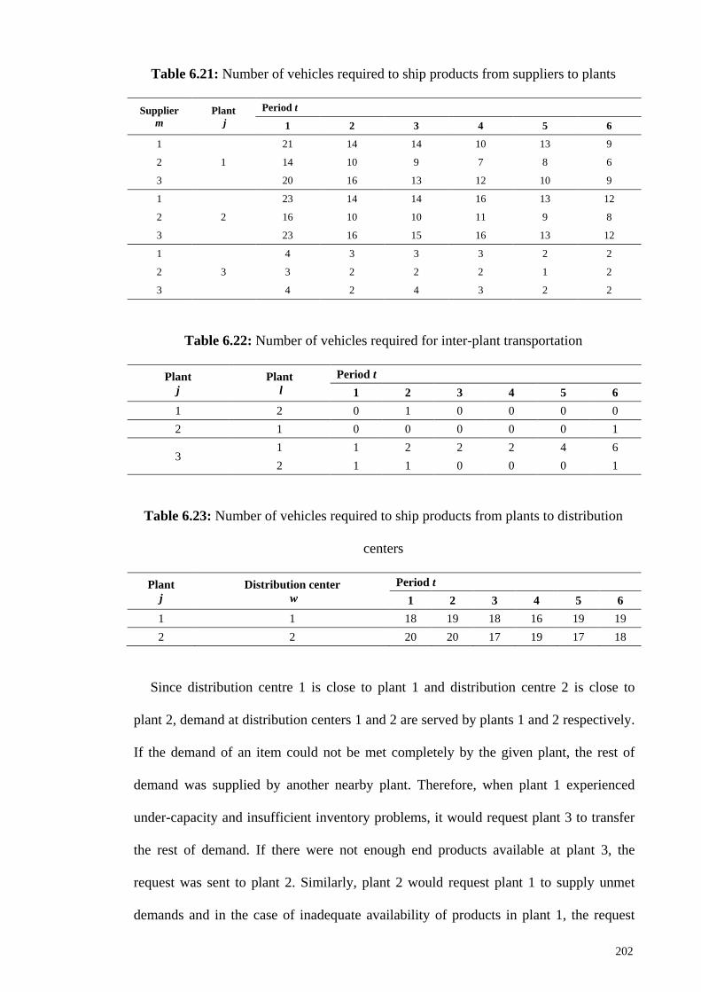
Table 6.21: Number of vehicles required to ship products from suppliers to plants
Supplier m
Plant j
Period t
1 2 3 4 5 6
1
1
21 14 14 10 13 9
2 14 10 9 7 8 6
3 20 16 13 12 10 9
1
2
23 14 14 16 13 12
2 16 10 10 11 9 8
3 23 16 15 16 13 12
1
3
4 3 3 3 2 2
2 3 2 2 2 1 2
3 4 2 4 3 2 2
Table 6.22: Number of vehicles required for inter-plant transportation
Plant j
Plant l
Period t 1 2 3 4 5 6
1 2 0 1 0 0 0 0 2 1 0 0 0 0 0 1
3 1 1 2 2 2 4 6 2 1 1 0 0 0 1
Table 6.23: Number of vehicles required to ship products from plants to distribution
centers
Plant j
Distribution center w
Period t 1 2 3 4 5 6
1 1 18 19 18 16 19 19 2 2 20 20 17 19 17 18
Since distribution centre 1 is close to plant 1 and distribution centre 2 is close to
plant 2, demand at distribution centers 1 and 2 are served by plants 1 and 2 respectively.
If the demand of an item could not be met completely by the given plant, the rest of
demand was supplied by another nearby plant. Therefore, when plant 1 experienced
under-capacity and insufficient inventory problems, it would request plant 3 to transfer
the rest of demand. If there were not enough end products available at plant 3, the
request was sent to plant 2. Similarly, plant 2 would request plant 1 to supply unmet
demands and in the case of inadequate availability of products in plant 1, the request
202
was then sent to plant 3. The results show that after all inter-plant transfers, demand at
both distribution centers could be entirely met during all periods.
Based on Table 6.19, the shortage cost incurred for distribution centers 1 and 2 in the
considered planning horizon is $53507, while the transportation cost is $51430. As
shortage cost is higher than the transportation and inventory costs, it indicates that
bearing some inventories or/and outsourcing from other plants is preferable than having
backorders. The reason lies in the fact that the cost of having backorder is far higher
than keeping inventory. In addition, meeting demand in a timely fashion increases
customer satisfaction.
The results also show that the binary variables ijtχ and kmjtϕ have value 1 for all
periods, indicating that the three different products were produced in each of three
plants and all plants have ordered all types of raw materials throughout the six-period
planning horizon.
6.7 Conclusions
This chapter investigated the effectiveness of coordinating production and
distribution planning by addressing a multi-item multi-period capacitated lot-sizing
problem in a multi-stage system composed of multiple suppliers, plants, and distribution
centers. The combinations of several functions were considered, such as purchasing,
production, storage, backordering, and transportation. The objective was to
simultaneously determine the optimal raw material order quantity, production and
inventory levels, and the transportation amount so that the demand can be satisfied with
the lowest possible cost over a given planning horizon without violating the capacity
restrictions of the plants and suppliers. Transfer decisions between plants were made
when demand observed at a plant was satisfied by other production sites to cope with
under-capacity of a given plant. Furthermore, sale at distribution centers was allowed.
203
A numerical example was described to demonstrate the validity of the proposed
model. Efficient search procedures were presented to obtain the optimum solutions by
employing four well-known metaheuristic algorithms, namely GA, PSO, ABC, and
ICA. In addition, Taguchi method was utilized to calibrate the various parameters of the
proposed algorithms. The GA method resulted in the best known solutions and
generated lower costs, and in general was found to be superior to other three
optimization approaches. In terms of number of function evaluations (computational
cost), the PSO was superior to the other methods. The results indicated that the
proposed model can provide a promising approach to fulfill an efficient production and
distribution planning in such integrated supply chain situations.
204
CHAPTER 7: CONCLUSIONS
7.1 Concluding Remarks
In this research, attempts were made to evaluate the efficiencies and benefits of using
a number of metaheuristic approaches for solving the lot-sizing and scheduling
problems. The implications of adding constraints to the economic lot scheduling
problem were discussed throughout this research. Generally, constraints regarding the
time-modeling increase the complexity of the problem leading to NP-hard situation
when such constraints are related to startup times between products. Capacity
restrictions also add more complexity to the lot-sizing problems.
Moreover, the capacitated lot-sizing problem was considered in the field of
integrated supply chain. The efficient management of supply chain has grown in
importance with the realization that it represents a major opportunity for organizations
to improve operational performance and overall margins.
In any manufacturing firm, the inventory management plays an essential role in
controlling the raw materials, work-in-processes and finished goods. If proper attention
is not given to choose efficient inventory policies, a significant amount of the
investment may be blocked in the inventory. Because of the heavy losses due to
excessive inventory or stockouts, more attention should be given in selecting an
effective inventory control system.
In this thesis, mathematical models were formulated and presented for solving the
single facility multiple item production problem, where products have shelf life
restrictions and can be backordered. The objective was to obtain the optimum cycle time
and to minimize the total related cost, including production, setup, holding, and
backordering costs. For the case where the optimal cycle time violated the shelf life
205
constraint, three adjustment options were investigated: production rate reduction, cycle
time reduction, and production rate and cycle time reduction simultaneously. It was
shown that parameters such as production cost, holding cost, setup cost, backorders, and
shelf life influence the decision making process to select the appropriate option that
offers the minimum yearly cost, and yields an optimum cycle time that satisfies shelf
life constraints.
In general, the production time cost exceeds the setup cost in many manufacturing
systems. Hence, it can be deduced that lowering cycle time is more cost-effective than
reducing the production rate. It was also revealed that in some circumstances, the option
of simultaneous reduction of the cycle time and production rate may offer the minimum
total cost comparable with adjusting only one of these two factors. Moreover,
considering planned backorders contributed to the lower total cost rather than models
with no backorders.
Thereafter, the scheduling optimization of a family of items for the economic lot
scheduling problem with shelf life restrictions, backordering, and multiple setups in a
production cycle was presented. The distinguishing feature of this work, compared to
previous studies, was allowing production of each item more than once in a cycle,
which brings about a significant reduction in the long run average cost. However, this
assumption may lead to an infeasible production schedule. Hence, to eliminate the
production time conflicts and to achieve feasibility, the schedule was adjusted by
advancing or delaying production start times of some batches of products. The objective
was to find the optimum production rate, production frequency, production quantity,
and cycle time for the family context so that the total cost including setup, holding,
backordering, and adjustment costs are minimized, and a feasible production schedule is
206
accommodated. It was shown that allowing multiple setups leads to improving
solutions.
Then, lot-sizing problem was investigated in a multi-plant environment. A multi-
plant supply chain is one in which a core exists simultaneously within several
manufacturing plants. Manufacturing facilities of the same supply chain should
coordinate planning and scheduling tasks and share the flow of information among
plants, upstream suppliers, and downstream distributors in order to enhance the whole
chain performance. The vital challenge is to define the interactions between different
levels of the manufacturing network at the planning and scheduling stage. In an
extended production network it is more difficult to manage all the necessary interactions
to ensure that disruptions and changes in one plant are taken into account by other
plants in order to prevent excessive inventory or stockouts.
Therefore, a mathematical model was presented for the multi-item multi-period
capacitated lot-sizing problem for an integrated production and distribution planning in
a multi-supplier multi-plant multi-distribution centre logistic environment. The products
were distributed to a number of distribution centers at which the demand for each
product was known for every period of the planning horizon. The bulk of operational
constraints were also represented in order to optimize the supply chain such as resource
utilization, demand fulfillment, production capacity, inventory storage capacity,
supplier capacity, and vehicle utilization. The goal was to minimize the total cost of the
supply chain including procurement, production, setup, inventory, backordering, and
transportation, and to meet demand in time. It was indicated that the proposed model
can provide a promising approach to fulfill an efficient production and distribution
planning in such integrated supply chain.
207
Since the proposed models are considered as NP-hard, the exact methods may fail to
solve them optimally. Hence, well-known metaheuristic algorithms namely genetic
algorithm, particle swarm optimization, artificial bee colony, simulated annealing, and
imperialist competitive algorithm were used to find the optimal or near-optimal
solutions within a moderate computation time. Metaheuristic methods have shown great
potentials for solving optimization problems as they conduct global stochastic search.
The reason of applying different algorithms to the proposed mathematical models was
to validate and to assess the quality of the obtained optimal solutions. It was shown that
for both ELSP and MPCLSP models, all applied methods obtained similar results,
which it confirms the correctness of the proposed models. In addition, Taguchi method
was used to calibrate the parameters of the metaheuristic methods. To compare the
performance of the proposed algorithms, the one-way ANOVA was conducted. The
statistical results showed that all presented algorithms can efficiently solve the proposed
models, while providing promising solutions with respect to solution quality compared
to those available in the literature. The metaheuristic algorithms can also handle large-
sized instances efficiently in a moderate CPU time.
However, for the proposed economic lot scheduling problem with multiple setups,
backordering, and shelf life considerations, ABC algorithm performed better than the
GA, PSO, and SA algorithms in terms of objective function value. In terms of CPU
time, SA was superior to the other algorithms. For the proposed multi-plant capacitated
lot-sizing problem, GA approach offered better results compared to PSO, ABC, and
ICA approaches in terms of objective function value. However, PSO algorithm offered
modest solution quality in less number of function evaluations for the proposed
problem.
208
7.2 Contributions and Applications
The developed mathematical models for the ELSP and MPCLSP incorporated a
variety of practical assumptions, and can cover a variety of problems arising in the
literature and in practice particularly scheduling, production and distribution.
It is common in industry to produce several products on a single facility (or machine)
due to economies of scale. Typically, these facilities can only produce one product at a
time, and have to be stopped and prepared (i.e. setup) at a cost of time and money,
before the start of the production run of a different product. A production scheduling
problem arises because of the need to coordinate the setups and the production runs of
the products. The ELSP is the problem of scheduling production of several products on
a single facility, so that demands are met without stockouts or backorders, and the long
run average inventory and setup costs are minimized. This problem occurs in many
production situations such as:
i. Metal forming and plastics production lines (press lines, and plastic and metal
extrusion machines), where each product requires a different die to be set up on
the machine.
ii. Assembly lines, which produce several products and/or different product models
(electric appliances, motor cars, etc.).
iii. Blending and mixing facilities (for paints, beverages, food, etc.), in which
different products are poured into different containers.
iv. Weaving production lines (for textiles, carpets, etc.), in which the main products
are manufactured in different colors, widths and grades.
Typically, it is more economical to purchase one high-speed machine capable of
producing a number of products than to purchase many dedicated machines.
209
The proposed MPCLSP model integrated the manufacturing and goods distribution
which mostly were considered as discrete problems in the previous studies available in
literature. However, in reality for most manufacturing environments, these problems are
interconnected. Shifting from single plant to multi-plant organization offers several
advantages such as saving on transportation cost and time, improving the customer
service by locating the plant close to the customer, being close to low cost raw
materials, flexibility in producing several products and specialization in activities,
substantial saving in global costs, improvement in relevant service by exploiting scale
economies of production and transportation, balancing production lots and vehicle
loads, reducing the inventory and stockouts, and so forth.
The MPCLSP can be observed in several industries such as automotive factories,
steel corporations, electric power generating industries, food and chemical process
industries, and beverage industry, where multiple plants producing the same products
are located at different geographical locations in a country or scattered around the
world.
Moreover, from the metaheuristic viewpoint, the contribution of the thesis was to
find out how metaheuristics performs for the MPCLSP, as previously they have been
applied mostly to other production related problems, in particular scheduling, but not to
this exact lot-sizing problem. The presented algorithms were computationally effective
and beneficial for obtaining the optimal solution for the proposed lot-sizing problems.
In any type of industry, the basic goal remains the same: to identify the most cost
effective or profitable way of getting the right product to the right place at the right time
in order to satisfy turbulent market demands.
210
7.3 Recommendations for Future Research
Future research may investigate the possibility of solving the proposed lot-sizing and
scheduling problems in stochastic manufacturing environments in which the uncertainty
and dynamic nature of some parameters are taken into account.
It may also be of interest to incorporate more realistic characteristic to the proposed
economic lot scheduling problem, such as machine failures in analysis of cyclic
schedules for products, unequal batches for each product as well as dissimilar
production cycles.
Moreover, in the proposed multi-plant capacitated lot-sizing problem, zero lead time
for production/replenishments was assumed in order to simplify the problem. Further
research may examine the relationship between lot sizes and lead times. Additionally,
safety stock for the products can also be integrated to the proposed lot-sizing problem as
it can have a significant impact on the firm’s performance.
211
REFERENCES
Abdelsalam, H. M., & Elassal, M. M. (2014). Joint economic lot-sizing problem for a three-layer supply chain with stochastic demand. International Journal of Production Economics, 155, 272-283.
Absi, N., & Kedad-Sidhoum, S. (2009). The multi-item capacitated lot-sizing problem with safety stocks and demand shortage costs. Computers & Operations Research, 36(11), 2926-2936.
Absi, N., Kedad-Sidhoum, S., & Dauzère-Pérès, S. (2011). Uncapacitated lot-sizing problem with production time windows, early productions, backlogs and lost sales. International Journal of Production Research, 49(9), 2551-2566.
Adelman, D., & Barz, C. (2013). A unifying approximate dynamic programming model for the economic lot scheduling problem. Mathematics of Operations Research, 39(2), 374-402.
Aghezzaf, E. H. (2007). Production planning and warehouse management in supply networks with inter-facility mold transfers. European Journal of Operational Research, 182(3), 1122-1139.
Agra, A., & Constantino, M. (1999). Lot-sizing with backlogging and start-ups: The case of Wagner-Whitin costs. Operations Research Letters, 25(2), 81-88.
Akay, B., & Karaboga, D. (2012). A modified artificial bee colony algorithm for real-parameter optimization. Information Sciences, 192, 120-142.
Akbalik, A., & Pochet, Y. (2009). Valid inequalities for the single-item capacitated lot-sizing problem with step-wise costs. European Journal of Operational Research, 198(2), 412-434.
Aksen, D., Altinkemer, K., & Chand, S. (2003). The single-item lot-sizing problem with immediate lost sales. European Journal of Operational Research, 147(3), 558-566.
Aksoy, Y., & Erenguc, S. S. (1988). Multi-item inventory models with co-ordinated replenishments: A survey. International Journal of Operations & Production Management, 8(1), 63-73.
Aliyu, M. D. S., & Andijani, A. A. (1999). Multi-item-multi-plant inventory control of production systems with shortages/backorders. International Journal of Systems Science, 30(5), 533-539.
Alvarez, E. (2007). Multi-plant production scheduling in SMEs. Robotics and Computer-Integrated Manufacturing, 23(6), 608-613.
Amorim, P., Günther, H. O., & Almada-Lobo, B. (2012). Multi-objective integrated production and distribution planning of perishable products. International Journal of Production Economics, 138(1), 89-101.
212
Anderson, E. J., Glass, C. A., & Potts, C. N. (1997). Machine scheduling. Local search in combinatorial optimization, 11, 361-414.
Anily, S., Tzur, M., & Wolsey, L. A. (2009). Multi-item lot-sizing with joint set-up costs. Mathematical programming, 119(1), 79-94.
Aras, Ö. A., & Swanson, L. A. (1982). A lot-sizing and sequencing algorithm for dynamic demands upon a single facility. Journal of Operations Management, 2(3), 177-185.
Armentano, V. A., Shiguemoto, A. L., & Løkketangen, A. (2011). Tabu search with path relinking for an integrated production–distribution problem. Computers & Operations Research, 38(8), 1199-1209.
Atashpaz-Gargari, E., & Lucas, C. (2007, September). Imperialist competitive algorithm: an algorithm for optimization inspired by imperialistic competition. In Evolutionary computation, 2007. CEC 2007. IEEE Congress on (pp. 4661-4667). IEEE.
Babaei, M., Mohammadi, M., & Ghomi, S. F. (2014). A genetic algorithm for the simultaneous lot sizing and scheduling problem in capacitated flow shop with complex setups and backlogging. The International Journal of Advanced Manufacturing Technology, 70(1-4), 125-134.
Bahl, H. C., Ritzman, L. P., & Gupta, J. N. (1987). OR practice-determining lot sizes and resource requirements: A review. Operations Research, 35(3), 329-345.
Barbarosoğlu, G., & Özdamar, L. (2000). Analysis of solution space-dependent performance of simulated annealing: the case of the multi-level capacitated lot-sizing problem. Computers & Operations Research, 27(9), 895-903.
Behnamian, J., & Ghomi, S. F. (2013). The heterogeneous multi-factory production network scheduling with adaptive communication policy and parallel machine. Information Sciences, 219, 181-196.
Belvaux, G., & Wolsey, L. A. (2000). Bc-prod: A specialized branch-and-cut system for lot-sizing problems. Management Science, 46(5), 724-738.
Ben-Daya, M., As’ad, R., & Seliaman, M. (2013). An integrated production inventory model with raw material replenishment considerations in a three layer supply chain. International Journal of Production Economics, 143(1), 53-61.
Berretta, R., & Rodrigues, L. F. (2004). A memetic algorithm for a multistage capacitated lot-sizing problem. International Journal of Production Economics, 87(1), 67-81.
Berretta, R., França, P. M., & Armentano, V. A. (2005). Metaheuristic approaches for the multilevel resource-constrained lot-sizing problem with setup and lead times. Asia-Pacific Journal of Operational Research, 22(02), 261-286.
Bhatnagar, R., Chandra, P., & Goyal, S. K. (1993). Models for multi-plant coordination. European Journal of Operational Research, 67(2), 141-160.
213
Billington, P. J., McClain, J. O., & Thomas, L. J. (1983). Mathematical programming approaches to capacity-constrained MRP systems: Review, formulation and problem reduction. Management Science, 29(10), 1126-1141.
Bitran, G. R., & Tirupati, D. (1993). Hierarchical production planning. Handbooks in operations research and management science, 4, 523-568.
Bitran, G. R., & Yanasse, H. H. (1982). Computational complexity of the capacitated lot size problem. Management Science, 28(10), 1174-1186.
Bollapragada, R., & Rao, U. (1999). Single-stage resource allocation and economic lot scheduling on multiple, non-identical production lines. Management Science, 45(6), 889-904.
Bollapragada, R., Della Croce, F., & Ghirardi, M. (2011). Discrete-time, economic lot scheduling problem on multiple, non-identical production lines. European Journal of Operational Research, 215(1), 89-96.
Bomberger, E. E. (1966). A dynamic programming approach to a lot size scheduling problem. Management Science, 12(11), 778-784.
Bourland, K. E., & Yano, C. A. (1994). The strategic use of capacity slack in the economic lot scheduling problem with random demand. Management Science, 40(12), 1690-1704.
Boussaïd, I., Lepagnot, J., & Siarry, P. (2013). A survey on optimization metaheuristics. Information Sciences, 237, 82-117.
Brahimi, N., Dauzere-Peres, S., Najib, N. M., & Nordli, A. (2006). Single item lot-sizing problems. European Journal of Operational Research, 168(1), 1-16.
Brander, P., & Forsberg, R. (2006). Determination of safety stocks for cyclic schedules with stochastic demands. International Journal of Production Economics, 104(2), 271-295.
Bruggeman, W., Vandendaele, P., & Muller, H. (1982). Diagnostic analysis of the potential savings of a multi-product/single facility production planning system. Engineering Costs and Production Economics, 6, 33-41.
Brüggemann, W., Jahnke, H. (1994). DLSP for two-stage multi-item batch production. International Journal of Production Research, 32(4), 755-768
Buer, T., Homberger, J., & Gehring, H. (2013). A collaborative ant colony metaheuristic for distributed multi-level uncapacitated lot-sizing. International Journal of Production Research, 51(17), 5253-5270.
Bulut, O., & Tasgetiren, M. F. (2014, July). A discrete artificial bee colony algorithm for the Economic Lot Scheduling problem with returns. In Evolutionary Computation (CEC), 2014 IEEE Congress on (pp. 551-557). IEEE.
Bulut, O., Tasgetiren, M. F., & Fadiloglu, M. M. (2012). A genetic algorithm for the economic lot scheduling problem under extended basic period approach and
214
power-of-two policy. In Advanced Intelligent Computing Theories and Applications. With Aspects of Artificial Intelligence (pp. 57-65). Springer Berlin Heidelberg.
Buschkühl, L., Sahling, F., Helber, S., & Tempelmeier, H. (2010). Dynamic capacitated lot-sizing problems: a classification and review of solution approaches. OR Spectrum, 32(2), 231-261.
Caserta, M., Ramirez, A., & Voß, S. (2010). A math-heuristic for the multi-level capacitated lot-sizing problem with carryover. In Applications of Evolutionary Computation (pp. 462-471). Springer Berlin Heidelberg.
Chakravarthy, S. R., & Daniel, J. K. (2004). A Markovian inventory system with random shelf time and back orders. Computers & Industrial Engineering, 47(4), 315-337.
Chan, F. T. S., Chung, S. H., Chan, P. L. Y., Finke, G., & Tiwary, M. K. (2005). Solving distributed scheduling problem with alternative routings by genetic algorithms. In 15th International Conference on Flexible Automation and Intelligent Manufacturing FAIM 2005 (pp. 391-399).
Chan, F. T. S., Kumar, V., & Mishra, N. (2008, September). Resolving multi plant supply chain problem: A novel swarm intelligence based approach. In Management of Innovation and Technology, 2008. ICMIT 2008. 4th IEEE International Conference on (pp. 1066-1071). IEEE.
Chan, F. T. S., Tibrewal, R. K., Prakash, A., & Tiwari, M. K. (2015). A biased random key genetic algorithm approach for inventory-based multi-item lot-sizing problem. Proceedings of the Institution of Mechanical Engineers, Part B: Journal of Engineering Manufacture, 229(1), 157-171.
Chandra, P., & Fisher, M. L. (1994). Coordination of production and distribution planning. European Journal of Operational Research, 72(3), 503-517.
Chandrasekaran, C., Rajendran, C., Krishnaiah Chetty, O., & Hanumanna, D. (2007). Metaheuristics for solving economic lot scheduling problems (ELSP) using time-varying lot-sizes approach. European Journal of Industrial Engineering, 1(2), 152-181.
Chatfield, D.C. (2007). The economic lot scheduling problem: A pure genetic search approach. Computers & Operations Research, 34(10), 2865-2881.
Chen, C. L. (2010, July). A heuristic model for justifying the acceptance of rush orders in multi-plants manufacturing supply chain with outsourcing. In Industrial Informatics (INDIN), 2010 8th IEEE International Conference on (pp. 607-611). IEEE.
Chen, H. (2015). Fix-and-optimize and variable neighborhood search approaches for multi-level capacitated lot-sizing problems. Omega, 56, 25-36.
215
Chen, H. D., Hearn, D. W., & Lee, C. Y. (1994). A new dynamic programming algorithm for the single item capacitated dynamic lot size model. Journal of Global Optimization, 4(3), 285-300.
Chen, H., & Chu, C. (2003). A Lagrangian relaxation approach for supply chain planning with order/setup costs and capacity constraints. Journal of Systems Science and Systems Engineering, 12(1), 98-110.
Chen, W. H., & Thizy, J. M. (1990). Analysis of relaxations for the multi-item capacitated lot-sizing problem. Annals of operations Research, 26(1), 29-72.
Chen, Y. Y., & Lin, J. T. (2009). A modified particle swarm optimization for production planning problems in the TFT Array process. Expert Systems with Applications, 36(10), 12264-12271.
Chen, Z., & Sarker, B. R. (2014). An integrated optimal inventory lot-sizing and vehicle-routing model for a multi-supplier single-assembler system with JIT delivery. International Journal of Production Research, 52(17), 5086-5114.
Chiu, S. W. (2008). Production lot size problem with failure in repair and backlogging derived without derivatives. European Journal of Operational Research, 188(2), 610-615.
Chopra, S., & Meindl, P. (2001). Supply chain management: strategy, planning, operation (1st Ed.). NJ, USA: Prentice Hall, Upper Saddle River.
Chowdhury, M. R., & Sarker, B. R. (2001). Manufacturing batch size and ordering policy for products with shelf lives. International Journal of Production Research, 39(7), 1405-1426.
Chung, C. S., Flynn, J., & Lin, C. H. M. (1994). An effective algorithm for the capacitated single item lot size problem. European Journal of Operational Research, 75(2), 427-440.
Chung, S. H., & Chan, H. K. (2012). A two-level genetic algorithm to determine production frequencies for economic lot scheduling problem. Industrial Electronics, IEEE Transactions on, 59(1), 611-619.
Clark, A., Almada-Lobo, B., & Almeder, C. (2011). Lot-sizing and scheduling: industrial extensions and research opportunities. International Journal of Production Research, 49(9), 2457-2461.
Coelho, L., & Sierakowski, C. A. (2008). A software tool for teaching of particle swarm optimization fundamentals. Advances in Engineering Software, 39(11), 877-887.
Conklin, J. M., & Perdue, B. A. (1994, May). Extending capabilities through contract manufacturing. In Electro/94 International. Conference Proceedings. Combined Volumes. (pp. 145-153). IEEE.
Cooper, M. C., Lambert, D. M., & Pagh, J. D. (1997). Supply chain management: more than a new name for logistics. The International Journal of Logistics Management, 8(1), 1-14.
216
Crowston, W. B., & Wagner, M. (1971). Lot size determination in multi-stage assembly systems. (Unpublished doctoral dissertation). Sloan School of Management, M. I. T., USA.
Dantzig, G. B. (1955). Optimal solution of a dynamic Leontief model with substitution. Econometrica: Journal of the Econometric Society, 295-302.
De Kok, T. G. (2000). Capacity allocation and outsourcing in a process industry. International Journal of Production Economics, 68(3), 229-239.
De Reyck, B. (2015). Period decompositions for the capacitated lot-sizing problem with setup times. Informs Journal on Computing.
De Souza, K. X., & Armentano, V. A. (1994). Multi-item capacitated lot-sizing by a cross decomposition based algorithm. Annals of Operations Research, 50(1), 557-574.
De Toledo, F. M. B., & Shiguemoto, A. L. (2005). Lot-sizing problem with several production centers. Pesquisa Operacional, 25(3), 479-492.
Dellaert, N. P., & Jeunet, J. (2003). Randomized multi-level lot-sizing heuristics for general product structures. European Journal of Operational Research, 148(1), 211-228.
Dellaert, N., & Jeunet, J. (2000). Solving large unconstrained multilevel lot-sizing problems using a hybrid genetic algorithm. International Journal of Production Research, 38(5), 1083-1099.
Dellaert, N., Jeunet, J., & Jonard, N. (2000). A genetic algorithm to solve the general multi-level lot-sizing problem with time-varying costs. International Journal of Production Economics, 68(3), 241-257.
DeMatteis, J. J. (1968). An economic lot-sizing technique, I: The part-period algorithm. IBM Systems Journal, 7(1), 30-38.
Dhaenens-Flipo, C. (2000). Spatial decomposition for a multi-facility production and distribution problem. International Journal of Production Economics, 64(1), 177-186.
Dhaenens-Flipo, C., & Finke, G. (2001). An integrated model for an industrial production–distribution problem. IIE Transactions, 33(9), 705-715.
Dhingra, A. K. (2006). Multi-objective flow shop scheduling using metaheuristics. (Unpublished doctoral dissertation). National Institute of Technology Kurukshetra.
Dixon, P. S., & Silver, E. A. (1981). A heuristic solution procedure for the multi-item, single-level, limited capacity, lot-sizing problem. Journal of Operations Management, 2(1), 23-39.
Dobson, G. (1987). The economic lot-scheduling problem: achieving feasibility using time-varying lot sizes. Operations Research, 35(5), 764-771.
217
Drexl, A., & Haase, K. (1995). Proportional lot-sizing and scheduling. International Journal of Production Economics, 40(1), 73-87.
Drexl, A., & Kimms, A. (1997). Lot-sizing and scheduling-survey and extensions. European Journal of Operational Research, 99(2), 221-235.
El-Alfy, E. S. M., Thampi, S. M., Takagi, H., Piramuthu, S., & Hanne, T. (2015). Advances in Intelligent Informatics. Springer.
Fakhrzad, M. B., & Zare, H. K. (2009). Combination of genetic algorithm with Lagrange multipliers for lot-size determination in multi-stage production scheduling problems. Expert Systems with Applications, 36(6), 10180-10187.
Federgruen, A., & Tzur, M. (1994). The joint replenishment problem with time-varying costs and demands: Efficient, asymptotic and ε-optimal solutions. Operations Research, 42(6), 1067-1086.
Federgruen, A., Meissner, J., & Tzur, M. (2007). Progressive interval heuristics for multi-item capacitated lot-sizing problems. Operations Research, 55(3), 490-502.
Fleischmann, B. (1990). The discrete lot-sizing and scheduling problem. European Journal of Operational Research, 44(3), 337-348.
Fleischmann, B., & Meyr, H. (1997). The general lot-sizing and scheduling problem. Operations-Research-Spektrum, 19(1), 11-21.
Florian, M., Lenstra, J.K., & Kan, A.R. (1980). Deterministic production planning: Algorithms and complexity. Management Science, 26(7), 669-679.
Fordyce, J. M., & Webster, F. M. (1985). Nonconstant unit cost/price with the Wagner-Whitin algorithm. Production and Inventory Management, 26(1), 71-80.
França, P. M., Armentano, V. A., Berretta, R. E., & Clark, A. R. (1997). A heuristic method for lot-sizing in multi-stage systems. Computers & Operations Research, 24(9), 861-874.
Fumero, F., & Vercellis, C. (1999). Synchronized development of production, inventory, and distribution schedules. Transportation science, 33(3), 330-340.
Gaafar, L.K., Nassef, A.O., & Aly, A.I. (2009). Fixed-quantity dynamic lot-sizing using simulated annealing. The International Journal of Advanced Manufacturing Technology, 41(1-2), 122-131.
Gallego, G., & Joneja, D. (1994). Economic lot scheduling problem with raw material considerations. Operations Research, 42(1), 92-101.
Ganeshan, R., Jack, E., Magazine, M. J., & Stephens, P. (1999). A taxonomic review of supply chain management research. In Quantitative models for supply chain management (pp. 839-879). Springer US.
218
Ganguly, S., Chowdhury, A., Mukherjee, S., Suganthan, P. N., Das, S., & Chua, T. J. (2013). A Hybrid Discrete Differential Evolution Algorithm for Economic Lot Scheduling Problem with Time Variant Lot-sizing. In Soft Computing Models in Industrial and Environmental Applications (pp. 1-12). Springer Berlin Heidelberg.
Gascon, A. (1995). On the finite horizon EOQ model with cost changes. Operations Research, 43, 716-717.
Gavish, B., & Johnson, R. E. (1990). A fully polynomial approximation scheme for single-product scheduling in a finite capacity facility. Operations Research, 38(1), 70-83.
Gen, M., Cheng, R., & Lin, L. (2008). Network models and optimization: Multi-objective genetic algorithm approach. Springer.
Gendreau, M., & Potvin, J. Y. (2005). Metaheuristics in combinatorial optimization. Annals of Operations Research, 140(1), 189-213.
Giri, B. C., Moon, I., & Yun, W. Y. (2003). Scheduling economic lot sizes in deteriorating production systems. Naval Research Logistics, 50(6), 650-661.
Glock, C. H., Grosse, E. H., & Ries, J. M. (2014). The lot-sizing problem: A tertiary study. International Journal of Production Economics, 155, 39-51.
Goetschalckx, M. (2011). Supply chain engineering. Springer Science & Business Media.
Goyal, S. K. (1994). A note on effect of production cost on shelf -life. International Journal of Production Research, 32(9), 2243-2245.
Goyal, S. K. (1996) A note on dealing with a shelf life constraint in cyclic scheduling by adjusting both cycle time and production rate. International Journal of Production Research, 34(10), 2967-2969.
Goyal, S. K., & Deshmukh, S. G. (1992). Integrated procurement-production systems: A review. European Journal of Operational Research, 62(1), 1-10.
Goyal, S. K., & Deshmukh, S. G. (1993). Discussion a note on ‘the economic ordering quantity for jointly replenishing items’. International Journal of Production Research, 31(12), 2959-2961.
Goyal, S. K., & Viswanathan, S. (2006). On ‘Optimal production policy with shelf life including shortages. Journal of Operational Research Society, 57, 747-747.
Graves, S. C. (1981). A review of production scheduling. Operations Research, 29(4), 646-675.
Guimarães, L., Klabjan, D., & Almada-Lobo, B. (2012). Annual production budget in the beverage industry. Engineering Applications of Artificial Intelligence, 25(2), 229-241.
219
Günther, H. O. (1987). Planning lot sizes and capacity requirements in a single stage production system. European Journal of Operational Research, 31(2), 223-231.
Gupta, C., & Jain, S. (2015). New Approach for Function Optimization: Amended Harmony Search. In Advances in Intelligent Informatics (pp. 643-653). Springer International Publishing.
Gupta, D., & Magnusson, T. (2005). The capacitated lot-sizing and scheduling problem with sequence-dependent setup costs and setup times. Computers & Operations Research, 32(4), 727-747.
Gupta, S. M., & Brennan, L. (1992). Heuristic and optimal approaches to lot-sizing incorporating backorders: an empirical evaluation. The International Journal of Production Research, 30(12), 2813-2824.
Gupta, S., & Karimi, I. A. (2003). Scheduling a two-stage multiproduct process with limited product shelf life in intermediate storage. Industrial & Engineering Chemistry Research, 42(3), 490-508.
Gürler, Ü., and Özkaya, B. Y. (2008) Analysis of the (s, S) policy for perishables with a random shelf life. IIE Transactions, 40, 759-781.
Gutiérrez, J., Sedeño-Noda, A., Colebrook, M., & Sicilia, J. (2008). An efficient approach for solving the lot-sizing problem with time-varying storage capacities. European Journal of Operational Research, 189(3), 682-693.
Haase, K. (1994). Lotsizing and scheduling for production planning, number 408 in Lecture Notes in Economics and Mathematical Systems, Springer, Berlin.
Haase, K. (1996). Capacitated lot-sizing with sequence dependent setup costs. Operations-Research-Spektrum, 18(1), 51-59.
Hajipour, V., Fattahi, P., & Nobari, A. (2014). A hybrid ant colony optimization algorithm to optimize capacitated lot-sizing problem. Journal of Industrial and Systems Engineering, 7(1), 1-20.
Hajipour, V., Kheirkhah, A., Tavana, M., & Absi, N. (2015). Novel Pareto-based meta-heuristics for solving multi-objective multi-item capacitated lot-sizing problems. The International Journal of Advanced Manufacturing Technology, 1-15.
Han, Y., Tang, J., Kaku, I., & Mu, L. (2009). Solving uncapacitated multilevel lot-sizing problems using a particle swarm optimization with flexible inertial weight. Computers & Mathematics with Applications, 57(11), 1748-1755.
Hardin, J. R., Nemhauser, G. L., & Savelsbergh, M. W. (2007). Analysis of bounds for a capacitated single-item lot-sizing problem. Computers & operations research, 34(6), 1721-1743.
Hariga, M. A. (1994). Economic analysis of dynamic inventory models with non-stationary costs and demand. International Journal of Production Economics, 36(3), 255-266.
220
Harris, F. W. (1913). How many parts to make at once. Operations Research, 947-950.
Hax, A., & Candea, D. (1984). Production and inventory management. Prentice-Hall, Englewood Cliffs, NJ.
Heizer, J., & Render, B. (2004). Operations Management. Upper Saddle River: Pearson Education.
Helber, S., & Sahling, F. (2010). A fix-and-optimize approach for the multi-level capacitated lot sizing problem. International Journal of Production Economics, 123(2), 247-256.
Hellion, B., Mangione, F., & Penz, B. (2012). A polynomial time algorithm to solve the single-item capacitated lot-sizing problem with minimum order quantities and concave costs. European Journal of Operational Research, 222(1), 10-16.
Hernandez, W., & Suer, G. (1999). Genetic algorithms in lot-sizing decisions. In Evolutionary Computation, 1999. CEC 99. Proceedings of the 1999 Congress on (Vol. 3). IEEE.
Hindi, K. S. (1995a). Solving the single-item, capacitated dynamic lot-sizing problem with startup and reservation costs by tabu search. Computers & industrial engineering, 28(4), 701-707.
Hindi, K. S. (1995b). Computationally efficient solution of the multi-item, capacitated lot-sizing problem. Computers & industrial engineering, 28(4), 709-719.
Hindi, K. S. (1996). Solving the CLSP by a tabu search heuristic. Journal of the Operational Research Society, 151-161.
Hindi, K. S., Fleszar, K., & Charalambous, C. (2003). An effective heuristic for the CLSP with set-up times. Journal of the Operational Research Society, 54(5), 490-498.
Holland, J. H. (1975). Adoption in neural and artificial systems. Ann Arbor, Michigan (USA): The University of Michigan Press.
Homberger, J. (2010). Decentralized multi-level uncapacitated lot-sizing by automated negotiation. 4OR, 8(2), 155-180.
Homberger, J., & Gehring, H. (2009, January). An ant colony optimization approach for the multi-level unconstrained lot-sizing problem. In System Sciences, 2009. HICSS'09. 42nd Hawaii International Conference on (pp. 1-7). IEEE.
Horng, S. C., & Yang, F. Y. (2013, January). Optimal base-stock level of the stochastic economic lot scheduling problem. In Computing, Management and Telecommunications (ComManTel), 2013 International Conference on (pp. 380-385). IEEE.
Hsu, W. L. (1983). On the general feasibility test of scheduling lot sizes for several products on one machine. Management science, 29(1), 93-105.
221
Hung, Y. F., & Chien, K. L. (2000). A multi-class multi-level capacitated lot-sizing model. Journal of the Operational Research Society, 51(11), 1309-1318.
Hwang, H. C., & van den Heuvel, W. (2009). Economic lot-sizing problem with bounded inventory and lost-sales (No. EI 2009-01, pp. 1-30). Econometric Institute Research Papers.
Hwang, H. C., Ahn, H. S., & Kaminsky, P. (2013). Basis paths and a polynomial algorithm for the multistage production-capacitated lot-sizing problem. Operations Research, 61(2), 469-482.
Inderfurth, K., Kovalyov, M. Y., Ng, C. T., & Werner, F. (2007). Cost minimizing scheduling of work and rework processes on a single facility under deterioration of reworkables. International Journal of Production Economics, 105(2), 345-356.
Jans, R., & Degraeve, Z. (2007). Meta-heuristics for dynamic lot-sizing: A review and comparison of solution approaches. European Journal of Operational Research, 177(3), 1855-1875.
Jans, R., & Degraeve, Z. (2008). Modeling industrial lot-sizing problems: A review. International Journal of Production Research, 46(6), 1619-1643.
Jenabi, M., Fatemi Ghomi, S. M. T., Torabi, S. A., & Karimi, B. (2007). Two hybrid meta-heuristics for the finite horizon ELSP in flexible flow lines with unrelated parallel machines. Applied Mathematics and Computation, 186(1), 230–245.
Jeunet, J., & Jonard, N. (2005). Single-point stochastic search algorithms for the multi-level lot-sizing problem. Computers & operations research, 32(4), 985-1006.
Jodlbauer, H. (2006). An approach for integrated scheduling and lot-sizing. European journal of Operational Research, 172(2), 386-400.
Jolayemi, J. K., & Olorunniwo, F. O. (2004). A deterministic model for planning production quantities in a multi-plant, multi-warehouse environment with extensible capacities. International Journal of Production Economics, 87(2), 99-113.
Junqueira, R. A., & Morabito, R. (2012). Production and logistics planning considering circulation taxes in a multi-plant seed corn company. Computers and Electronics in Agriculture, 84, 100-110.
Karaboga, D. (2005). An idea based on honey bee swarm for numerical optimization (Vol. 200). Technical report-tr06, Erciyes University, Engineering Faculty, Computer Engineering Department.
Karaboga, D., & Basturk, B. (2008). Artificial Bee Colony (ABC) optimization algorithm for solving constrained optimization problems. Advances in Soft Computing, 8(1), 687-697.
Karimi, B., Fatemi Ghomi, S., & Wilson, J. (2003). The capacitated lot-sizing problem: a review of models and algorithms. Omega, 31(5), 365-378.
222
Karmarkar, U. S., & Schrage, L. (1985). The deterministic dynamic product cycling problem. Operations Research, 33(2), 326-345.
Kayvanfar, V., & Zandieh, M. (2012). The economic lot scheduling problem with deteriorating items and shortage: an imperialist competitive algorithm. The International Journal of Advanced Manufacturing Technology, 62(5-8), 759-773.
Kazaz, B., and Sloan, T. W. (2008) Production policies under deteriorating process conditions. IIE Transactions, 40, 187-205.
Kennedy J.F., & Eberhart, R.C. Particle swarm optimization. In: Proceedings of the IEEE international conference on neural networks, vol. 4. Perth, Australia; 1995, (pp. 1942–48).
Khouja, M., Michalewicz, Z., & Wilmot, M. (1998). The use of genetic algorithms to solve the economic lot size scheduling problem. European Journal of Operational Research, 110(3), 509-524.
Khoury, B. N., Abboud, N. E., & Tannous, M. M. (2001). The common cycle approach to the ELSP problem with insufficient capacity. International Journal of Production Economics, 73(2), 189-199.
Kimms, A. (1996). Competitive methods for multi-level lot-sizing and scheduling: tabu search and randomized regrets. International Journal of Production Research, 34(8), 2279-2298
Kirca, Ö. (1990). An efficient algorithm for the capacitated single item dynamic lot size problem. European Journal of Operational Research, 45, 15-24.
Kirca, Ö. (1995). A primal‐dual algorithm for the dynamic lot-sizing problem with joint set‐up costs. Naval Research Logistics, 42(5), 791-806.
Kirkpatrick, S. (1984). Optimization by simulated annealing: Quantitative studies. Journal of Statistical Physics, 34(5-6), 975-986.
Kirkpatrick, S., Gelatt, C. D., & Vecchi, M. P. (1983). Optimization by simulated annealing. Science, 220(4598), 671-680.
Koçlar, A., & Süral, H. (2005). A note on “The general lot-sizing and scheduling problem”. OR Spectrum, 27(1), 145-146.
Köksoy, O., & Yalcinoz, T. (2008). Robust Design using Pareto type optimization: A genetic algorithm with arithmetic crossover. Computers & Industrial Engineering, 55(1), 208-218.
Kreipl, S., & Pinedo, M. (2004). Planning and scheduling in supply chains: an overview of issues in practice. Production and Operations Management, 13(1), 77-92.
Kuhn, H. (1997). A dynamic lot-sizing model with exponential machine breakdowns. European Journal of Operational Research, 100(3), 514-536.
223
Kuik, R., Salomon, M., van Wassenhove, L. N., & Maes, J. (1993). Linear programming, simulated annealing and tabu search heuristics for lot sizing in bottleneck assembly systems. IIE transactions, 25(1), 62-72.
Kumar, S. A., & Suresh, N. (2009). Operations management. New Age International (P) Limited Publishers.
Lambrecht, M. R., & Vanderveken, H. (1979). Heuristic procedures for the single operation, multi-item loading problem. AIIE Transactions, 11(4), 319-326.
Lang, J. C. (2010). Production and inventory management with substitutions. Lecture Notes in Economics and Mathematical Systems 636, Springer, Berlin.
Lee, C. Y., Çetinkaya, S., & Wagelmans, A. P. (2001). A dynamic lot-sizing model with demand time windows. Management Science, 47(10), 1384-1395.
Lee, K. S., & Geem, Z. W. (2005). A new meta-heuristic algorithm for continuous engineering optimization: harmony search theory and practice. Computer methods in applied mechanics and engineering, 194(36), 3902-3933.
Lev, B., & Weiss, H. J. (1990). Inventory models with cost changes. Operations research, 38(1), 53-63.
Lin, H. C., Su, C. T., Wang, C. C., Chang, B. H., & Juang, R. C. (2012). Parameter optimization of continuous sputtering process based on Taguchi methods, neural networks, desirability function, and genetic algorithms. Expert Systems with Applications, 39(17), 12918-12925.
Lin, J. T., & Chen, Y. Y. (2007). A multi-site supply network planning problem considering variable time buckets-A TFT-LCD industry case. The International Journal of Advanced Manufacturing Technology, 33(9-10), 1031-1044.
Liu, J., Wu, L., & Zhou, Z. (2008). A time-varying lot size method for the economic lot scheduling problem with shelf life considerations. European Journal of Industrial Engineering, 2(3), 337-355.
Liu, X., Chu, F., Chu, C., & Wang, C. (2004). Some new properties for capacitated lot-sizing problem with bounded inventory and stockouts. WSEAS Transactions on Mathematics, 3, 65-70.
Löhndorf, N., Riel, M., & Minner, S. (2014). Simulation optimization for the stochastic economic lot scheduling problem with sequence-dependent setup times. International Journal of Production Economics, 157, 170-176.
Loparic, M., Pochet, Y., & Wolsey, L. A. (2001). The uncapacitated lot-sizing problem with sales and safety stocks. Mathematical Programming, 89(3), 487-504.
Lopez, M. A. N., & Kingsman, B. G. (1991). The economic lot scheduling problem: theory and practice. International Journal of Production Economics, 23(1), 147-164.
224
Lotfi, V., & Yoon, Y. S. (1994). An algorithm for the single-item capacitated lot-sizing problem with concave production and holding costs. Journal of the Operational Research Society, 934-941.
Lütke Entrup, M., Günther, H. O., Van Beek, P., Grunow, M., & Seiler, T. (2005). Mixed-integer linear programming approaches to shelf life-integrated planning and scheduling in yoghurt production. International Journal of Production Research, 43(23), 5071-5100.
Madić, M., Marković, D., & Radovanović, M. (2013). Comparison of meta-heuristic algorithms for solving machining optimization problems. Facta Universitatis Series: Mechanical Engineering, 11(1), 29-44.
Maes, J., & Van Wassenhove, L. (1988). Multi-item single-level capacitated dynamic lot-sizing heuristics: A general review. Journal of the Operational Research Society, 991-1004.
Maes, J., McClain, J. O., & Van Wassenhove, L. N. (1991). Multilevel capacitated lot-sizing complexity and LP-based heuristics. European Journal of Operational Research, 53(2), 131-148.
Mallya, R. (1992). Multi-product scheduling on a single machine: a case study. Omega, 20(4), 529-534.
Marinelli, F., Nenni, M. E., & Sforza, A. (2007). Capacitated lot-sizing and scheduling with parallel machines and shared buffers: A case study in a packaging company. Annals of Operations Research, 150(1), 177-192.
Maritan, C. A., Brush, T. H., & Karnani, A. G. (2004). Plant roles and decision autonomy in multinational plant networks. Journal of Operations Management, 22(5), 489-503.
Martin, C. H., Dent, D. C., & Eckhart, J. C. (1993). Integrated production, distribution, and inventory planning at Libbey-Owens-Ford. Interfaces, 23(3), 68-78.
McCarthy, I., & Anagnostou, A. (2004). The impact of outsourcing on the transaction costs and boundaries of manufacturing. International Journal of Production Economics, 88(1), 61-71.
Mehdizadeh, E., & Fatehi Kivi, A. (2014). Three Metaheuristic Algorithms for Solving the Multi-item Capacitated Lot-sizing Problem with Product Returns and Remanufacturing. Journal of Optimization in Industrial Engineering, 7(16), 41-53.
Millar, H. H., & Yang, M. (1994). Lagrangian heuristics for the capacitated multi-item lot-sizing problem with backordering. International Journal of Production Economics, 34(1), 1-15.
Mitchell, M. (1996). An introduction to genetic algorithms, 1996. PHI Pvt. Ltd., New Delhi.
225
Mohammadi, M., Ghomi, S. M. T., Karimi, B., & Torabi, S. A. (2009). Development of heuristics for multi-product multi-level capacitated lot-sizing problem with sequence-dependent setups. Journal of Applied Sciences, 9(2), 296–303.
Moon, C., Kim, J., & Hur, S. (2002). Integrated process planning and scheduling with minimizing total tardiness in multi-plants supply chain. Computers & Industrial Engineering, 43(1), 331-349.
Moon, I., Giri, B., & Choi, K. (2002a). Economic lot scheduling problem with imperfect production processes and setup times. Journal of the Operational Research Society, 53(6), 620-629.
Moon, I., Silver, E. A., & Choi, S. (2002b). Hybrid genetic algorithm for the economic lot-scheduling problem. International Journal of Production Research, 40(4), 809-824.
Mousavi, S. M., Hajipour, V., Niaki, S. T. A., & Aalikar, N. (2014). A multi-product multi-period inventory control problem under inflation and discount: a parameter-tuned particle swarm optimization algorithm. The International Journal of Advanced Manufacturing Technology, 70(9-12), 1739-1756.
Nascimento, M. C., & Toledo, F. (2008). A hybrid heuristic for the multi-plant capacitated lot-sizing problem with setup carry-over. Journal of the Brazilian Computer Society, 14(4), 7-15.
Nascimento, M.C., Resende, M.G., & Toledo, F. (2010). GRASP heuristic with path-relinking for the multi-plant capacitated lot-sizing problem. European Journal of Operational Research, 200(3), 747-754.
Nazari-Shirkouhi, S., Eivazy, H., Ghodsi, R., Rezaie, K., & Atashpaz-Gargari, E. (2010). Solving the integrated product mix-outsourcing problem using the imperialist competitive algorithm. Expert Systems with Applications, 37(12), 7615-7626.
Nilsson, K., & Segerstedt, A. (2008). Corrections of costs to feasible solutions of economic lot scheduling problems. Computers & Industrial Engineering, 54(1), 155-168.
Oliver, R. K., & Webber, M. D. (1982). Supply-chain management: logistics catches up with strategy. Outlook, 5(1), 42-47.
Osman, I. H., & Laporte, G. (1996). Metaheuristics: A bibliography. Annals of Operations research, 63(5), 511-623.
Özdamar, L., & Barbarosoğlu, G. (1999). Hybrid heuristics for the multi-stage capacitated lot-sizing and loading problem. Journal of the Operational Research Society, 50(8), 810-825.
Özdamar, L., & Barbarosoğlu, G. (2000). An integrated Lagrangian relaxation-simulated annealing approach to the multi-level multi-item capacitated lot-sizing problem. International Journal of Production Economics, 68(3), 319-331.
226
Özdamar, L., & Bozyel, M. A. (2000). The capacitated lot-sizing problem with overtime decisions and setup times. IIE Transactions, 32(11), 1043-1057.
Özdamar, L., Bilbil, Ş. İ., & Portmann, M. C. (2002). Technical note: New results for the capacitated lot-sizing problem with overtime decisions and setup times.
Pal, B., Sana, S. S., & Chaudhuri, K. (2012). A three layer multi-item production–inventory model for multiple suppliers and retailers. Economic Modelling, 29(6), 2704-2710.
Pan, Q. K., Tasgetiren, M. F., Suganthan, P. N., & Chua, T. J. (2011). A discrete artificial bee colony algorithm for the lot-streaming flow shop scheduling problem. Information sciences, 181(12), 2455-2468.
Pan, Z., Tang, J., & Liu, O. (2009). Capacitated dynamic lot-sizing problems in closed-loop supply chain. European Journal of Operational Research, 198(3), 810-821.
Park, Y. B. (2005). An integrated approach for production and distribution planning in supply chain management. International Journal of Production Research, 43(6), 1205-1224.
Parsapoor, M., & Bilstrup, U. (2012). Using the grouping genetic algorithm (GGA) for channel assignment in a cluster-based mobile ad hoc network. In Proceedings of SNCNW 2012: The 8th Swedish National Computer Networking Workshop: Stockholm, June 7-8, 2012 (pp. 56-60).
Parsapoor, M., & Bilstrup, U. (2013, December). School of Information Science, Computer and Electrical Engineering (IDE), Halmstad University, Sweden. In Wireless Sensor (ICWISE), 2013 IEEE Conference on (pp. 73-78). IEEE.
Pasandideh, S. H. R., & Niaki, S. T. A. (2008). A genetic algorithm approach to optimize a multi-products EPQ model with discrete delivery orders and constrained space. Applied Mathematics and Computation, 195(2), 506-514.
Peixin, Z. (2012). An Improved Particle Swarm Optimization Algorithm for the Economic Lot Scheduling Problem under Power-of-Two Policy. Advances in Information Sciences & Service Sciences, 4(20).
Phadke, M. S. (1989). Quality Engineering Using Robust Design, PTR Prentice-Hall. Inc., Englewood Cliffs, NJ.
Pirkul, H., & Jayaraman, V. (1998). A multi-commodity, multi-plant, capacitated facility location problem: formulation and efficient heuristic solution. Computers & Operations Research, 25(10), 869-878.
Pitakaso, R., Almeder, C., Doerner, K. F., & Hartl, R. F. (2006). Combining exact and population-based methods for the constrained multilevel lot-sizing problem. International Journal of Production Research, 44(22), 4755-4771.
Pitakaso, R., Almeder, C., Doerner, K. F., & Hartl, R. F. (2007). A MAX-MIN ant system for unconstrained multi-level lot-sizing problems. Computers & Operations Research, 34(9), 2533-2552.
227
Pochet, Y. (2001). Mathematical programming models and formulations for deterministic production planning problems. In Computational combinatorial optimization (pp. 57-111). Springer Berlin Heidelberg.
Prasad, P. S. S., & Chetty, O. K. (2001). Multilevel lot-sizing with a genetic algorithm under fixed and rolling horizons. The International Journal of Advanced Manufacturing Technology, 18(7), 520-527.
Quadt, D., & Kuhn, H. (2008). Capacitated lot-sizing with extensions: A review. Quarterly Journal of Operations Research, 6(1), 61-83.
Ramezanian, R., & Saidi-Mehrabad, M. (2013). Hybrid simulated annealing and MIP-based heuristics for stochastic lot-sizing and scheduling problem in capacitated multi-stage production system. Applied Mathematical Modelling, 37(7), 5134-5147.
Ramezanian, R., Saidi-Mehrabad, M., & Teimoury, E. (2013). A mathematical model for integrating lot-sizing and scheduling problem in capacitated flow shop environments. The International Journal of Advanced Manufacturing Technology, 66(1-4), 347-361.
Raza, A.S., Akgunduz, A., & Chen, M. (2006). A tabu search algorithm for solving economic lot scheduling problem. Journal of Heuristics, 12(6), 413-426.
Raza, A.S., & Akgunduz, A. (2008). A comparative study of heuristic algorithms on economic lot scheduling problem. Computers & Industrial Engineering, 55(1), 94-109.
Richter, K., & Sombrutzki, M. (2000). Remanufacturing planning for the reverse Wagner/Whitin models. European Journal of Operational Research, 121(2), 304-315.
Rizk, N. A. F. E. E., & Martel, A. (2001). Supply chain flow planning methods: A review of the lot-sizing literature. (Unpublished doctoral dissertation). Université Laval, Quebec City, Canada.
Rogers, J. (1958). A computational approach to the economic lot scheduling problem. Management Science, 4(3), 264-291.
Ruiz-Torres, A. J., Ho, J. C., & Lopez, F. J. (2006). Generating Pareto schedules with outsource and internal parallel resources. International Journal of Production Economics, 103(2), 810-825.
Sadeghi, J., Mousavi, S. M., Niaki, S. T. A., & Sadeghi, S. (2013). Optimizing a multi-vendor multi-retailer vendor managed inventory problem: Two tuned meta-heuristic algorithms. Knowledge-Based Systems, 50, 159-170.
Sadollah, A., Mohamed, M. N. H., & Bahreininejad, A. (2013). Optimum culture conditions for 1,3-Propanediol production from Crude Glycerol using metaheuristic algorithms. Applied Mathematics & Information Sciences, 1, 1-8.
228
Saka, M. P., Doğan, E., & Aydogdu, I. (2013). Analysis of Swarm Intelligence–Based Algorithms for Constrained Optimization. Swarm Intelligence and Bio-Inspired Computation, 25-48.
Salomon, M., Kroon, L. G., Kuik, R., & Van Wassenhove, L. N. (1991). Some extensions of the discrete lot-sizing and scheduling problem. Management Science, 37(7), 801-812.
Salvietti, L., & Smith, N. R. (2008). A profit-maximizing economic lot scheduling problem with price optimization. European Journal of Operational Research, 184(3), 900-914.
Salvietti, L., Smith, N. R., & Cárdenas-Barrón, L. E. (2014). A stochastic profit-maximizing economic lot scheduling problem with price optimization. European Journal of Industrial Engineering, 8(2), 193-221.
Sambasivan, M., & Schmidt, C. P. (2002). A heuristic procedure for solving multi-plant, multi-item, multi-period capacitated lot-sizing problems. Asia Pacific Journal of Operational Research, 19(1), 87-106.
Sambasivan, M., & Yahya, S. (2005). A Lagrangian-based heuristic for multi-plant, multi-item, multi-period capacitated lot-sizing problems with inter-plant transfers. Computers & Operations Research, 32(3), 537-555.
Sana, S. S. (2010). An economic production lot size model in an imperfect production system. European Journal of Operational Research, 201(1), 158-170.
Sana, S. S., Chedid, J. A., & Navarro, K. S. (2014). A three layer supply chain model with multiple suppliers, manufacturers and retailers for multiple items. Applied Mathematics and Computation, 229, 139-150.
Sandbothe, R. A., & Thompson, G. L. (1990). A forward algorithm for the capacitated lot size model with stockouts. Operations Research, 38(3), 474-486.
Sarker, B. R., and Babu, P. S. (1993) Effect of production cost on shelf life. International Journal of Production Research, 31(8), 1865-1872.
Sarker, B. R., Rochanaluk, R., & Egbelu, P. J. (2013). Improving service rate for a tree-type three-echelon supply chain system with backorders at retailer’s level. Journal of the Operational Research Society, 65(1), 57-72.
Senyiğit, E. (2010). New heuristics to stochastic dynamic lot-sizing problem. Gazi University Journal of Science, 22(2), 97-106.
Sharma, S. (2004). Optimal production policy with shelf life including shortages. Journal of the Operational Research Society, 55(8), 902-909.
Sharma, S. (2006). Incorporating fractional backordering in the multi-product manufacturing situation with shelf-lives. Journal of Engineering Manufacture, 220(7), 1151-1156.
229
Shaw, D. X., & Wagelmans, A. P. (1998). An algorithm for single-item capacitated economic lot-sizing with piecewise linear production costs and general holding costs. Management Science, 44(6), 831-838.
Silver, E. A. (1989). Shelf life considerations in a family production context. International Journal of Production Research, 27(12), 2021-2026.
Silver, E. A. (1995). Dealing with a shelf life constraint in cyclic scheduling by adjusting both the cycle time and production rate. International Journal of Production Research, 33(3), 623–629.
Silver, E. A., & Meal, H. C. (1973). A heuristic for selecting lot size quantities for the case of a deterministic time-varying demand rate and discrete opportunities for replenishment. Production and Inventory Management, 14(2), 64-74.
Soman, C. A., Van Donk, D. P., & Gaalman, G. (2004). Combined make-to-order and make-to-stock in a food production system. International Journal of Production Economics, 90(2), 223–135.
Song, Y., & Chan, G. H. (2005). Single item lot-sizing problems with backlogging on a single machine at a finite production rate. European Journal of Operational Research, 161(1), 191-202.
Stadtler, H. (1997). Reformulations of the shortest route model for dynamic multi-item multi-level capacitated lot-sizing. Operations-Research-Spektrum, 19(2), 87-96.
Suerie, C., & Stadtler, H. (2003). The capacitated lot-sizing problem with linked lot sizes. Management Science, 49(8), 1039-1054.
Sun, H., Huang, H. C., & Jaruphongsa, W. (2009). A genetic algorithm for the economic lot scheduling problem under the extended basic period and power-of-two policy. CIRP Journal of Manufacturing Science and Technology, 2(1), 29-34.
Swamidass, P. M. (Ed.). (2000). Encyclopedia of production and manufacturing management. Springer Science & Business Media.
Talbi, E. G. (2009). Metaheuristics: from design to implementation. John Wiley & Sons.
Tang, O. (2004). Simulated annealing in lot-sizing problems. International Journal of Production Economics, 88(2), 173-181.
Tang, O., & Teunter, R. (2006). Economic lot scheduling problem with returns. Production and Operations Management, 15(4), 488-497.
Tasgetiren, M. F., Bulut, O., & Murat Fadiloglu, M. (2011, June). A discrete artificial bee colony algorithm for the economic lot scheduling problem. In Evolutionary Computation (CEC), 2011 IEEE Congress on (pp. 347-353). IEEE.
Tasgetiren, M. F., Bulut, O., & Murat Fadiloglu, M. (2012, June). A discrete harmony search algorithm for the economic lot scheduling problem with power of two
230
policy. In Evolutionary Computation (CEC), 2012 IEEE Congress on (pp. 1-8). IEEE.
Tempelmeier, H. (1997). Resource-constrained materials requirements planning-MRP rc. Production Planning & Control, 8(5), 451-461.
Tempelmeier, H., & Hilger, T. (2015). Linear programming models for a stochastic dynamic capacitated lot-sizing problem. Computers & Operations Research, 59, 119-125.
Tersine, R. J., & Barman, S. (1991). Economic inventory/transport lot, sizing with quantity and freight rate discounts. Decision Sciences, 22(5), 1171-1179.
Teunter, R. H., & Flapper, S. D. P. (2003). Lot-sizing for a single-stage single-product production system with rework of perishable production defectives. OR Spectrum, 25(1), 85-96.
Teunter, R., Tang, O., & Kaparis, K. (2009). Heuristics for the economic lot scheduling problem with returns. International Journal of Production Economics, 118(1), 323-330.
Thizy, J. M., & Van Wassenhove, L. N. (1985). Lagrangian relaxation for the multi-item capacitated lot-sizing problem: A heuristic implementation. IIE transactions, 17(4), 308-313.
Thomas, D. J., & Griffin, P. M. (1996). Coordinated supply chain management. European Journal of Operational Research, 94(1), 1-15.
Toledo, C. F. M., de Oliveira, L., de Freitas Pereira, R., França, P. M., & Morabito, R. (2014). A genetic algorithm/mathematical programming approach to solve a two-level soft drink production problem. Computers & Operations Research, 48, 40-52.
Toledo, C. F. M., De Oliveira, R. R. R., & França, P. M. (2013). A hybrid multi-population genetic algorithm applied to solve the multi-level capacitated lot-sizing problem with backlogging. Computers & Operations Research, 40(4), 910-919.
Torabi, S. A., Karimi, B., & Ghomi, S. F. (2005). The common cycle economic lot scheduling in flexible job shops: The finite horizon case. International Journal of Production Economics, 97(1), 52-65.
Tseng, Y. J., Chen, J. Y., & Huang, F. Y. (2010a). A multi-plant assembly sequence planning model with integrated assembly sequence planning and plant assignment using GA. The International Journal of Advanced Manufacturing Technology, 48(1-4), 333-345.
Tseng, Y. J., Chen, J. Y., & Huang, F. Y. (2010b). A particle swarm optimization algorithm for multi-plant assembly sequence planning with integrated assembly sequence planning and plant assignment. International Journal of Production Research, 48(10), 2765-2791.
231
Tukel, O. I., & Wasti, S. N. (2001). Analysis of supplier buyer relationships using resource constrained project scheduling strategies. European Journal of Operational Research, 129(2), 271-276.
Van Eijs, M. J. G., Heuts, R. M. J., & Kleijnen, J. P. C. (1992). Analysis and comparison of two strategies for multi-item inventory systems with joint replenishment costs. European Journal of Operational Research, 59(3), 405-412.
Vargas, V. (2009). An optimal solution for the stochastic version of the Wagner-Whitin dynamic lot-size model. European Journal of Operational Research, 198(2), 447-451.
Viswanathan, S. (1995). A note on effect of production cost on shelf life. International Journal of Production Research, 33(12), 3485-3486.
Viswanathan, S., & Goyal, S. K. (2000). Incorporating planned backorders in a family production context with shelf life considerations. International Journal of Production Research, 38(4), 829–836.
Viswanathan, S., & Goyal, S. K. (2002). Technical note on manufacturing batch size and ordering policy for products with shelf lives. International Journal of Production Research, 40(8), 1965-1970.
Viswanathan, S., and Goyal, S. K. (1997). Optimal cycle time and production rate in a family production context with shelf life considerations. International Journal of Production Research, 35(6), 1703-1711.
Vorst, J. G. A. J. V. D. (2000). Effective food supply chains: generating, modeling and evaluating supply chain scenarios. Wageningen Universiteit.
Voß, S., Martello, S., Osman, I. H., & Roucairol, C. (Eds.). (2012). Meta-heuristics: Advances and trends in local search paradigms for optimization. Springer Science & Business Media.
Wagner, H. M., & Whitin, T. M. (1958). Dynamic version of the economic lot size model. Management Science, 5(1), 89-96.
Wild, R. (1974). The origins and development of flow-line production. Industrial Archaeology, 11(1-3), 43-55.
Woarawichai, C., Kullpattaranirun, T., & Rungreunganun, V. (2010). Applying genetic algorithms for inventory lot-sizing problem with supplier selection under storage space. Asian International Journal of Science and Technology in Production and Manufacturing Engineering, 3(4), 37-45.
Wolpert, D. H., & Macready, W. G. (1997). No free lunch theorems for optimization. Evolutionary Computation, IEEE Transactions on, 1(1), 67-82.
Wu, T., & Shi, L. (2011). Mathematical models for capacitated multi-level production planning problems with linked lot sizes. International Journal of Production Research, 49(20), 6227-6247.
232
Wu, T., Shi, L., Geunes, J., & Akartunalı, K. (2011). An optimization framework for solving capacitated multi-level lot-sizing problems with backlogging. European Journal of Operational Research, 214(2), 428-441.
Xie, J., & Dong, J. (2002). Heuristic genetic algorithms for general capacitated lot-sizing problems. Computers & Mathematics with applications, 44(1), 263-276.
Xu, Y., & Sarker, B. R. (2003). Models for a family of products with shelf life and production and shortage costs in emerging markets. Computers & Operations Research, 30(6), 925-938.
Yaghini, M., & Khandaghabadi, Z. (2013). A hybrid metaheuristic algorithm for dynamic rail car fleet sizing problem. Applied Mathematical Modelling, 37(6), 4127-4138.
Yan, C., Banerjee, A., & Yang, L. (2011). An integrated production–distribution model for a deteriorating inventory item. International Journal of Production Economics, 133(1), 228-232.
Yan, C., Liao, Y., & Banerjee. A. (2013). Multi-product lot scheduling with backordering and shelf life constraints. Omega, 41(3), 510-516.
Yang, F. C., Chen, K., Wang, M. T., Chang, P. Y., & Sun, K. C. (2010). Mathematical modeling of multi-plant order allocation problem and solving by genetic algorithm with matrix representation. The International Journal of Advanced Manufacturing Technology, 51(9-12), 1251-1259.
Yao, M. J., & Huang, J. X. (2005). Solving the economic lot scheduling problem with deteriorating items using genetic algorithms. Journal of Food Engineering, 70(3), 309-322.
Yazdani, M., Gohari, S., & Naderi, B. (2015). Multi-factory parallel machine problems: Improved mathematical models and artificial bee colony algorithm. Computers & Industrial Engineering, 81, 36-45.
Zangwill, W. I. (1969). A backlogging model and a multi-echelon model of a dynamic economic lot size production system-a network approach. Management Science, 15(9), 506-527.
Zanoni, S., Segerstedt, A., Tang, O., & Mazzoldi, L. (2012). Multi-product economic lot scheduling problem with manufacturing and remanufacturing using a basic period policy. Computers & Industrial Engineering, 62(4), 1025-1033.
Zhang, Z. H., Jiang, H., & Pan, X. (2012). A Lagrangian relaxation based approach for the capacitated lot-sizing problem in closed-loop supply chain. International Journal of Production Economics, 140(1), 249-255.
Zhong, Y., & Pan, X. (2007, August). A hybrid optimization solution to VRPTW based on simulated annealing. In Automation and Logistics, 2007 IEEE International Conference on (pp. 3113-3117). IEEE.
233

Zipkin, P. H. (1991). Computing optimal lot sizes in the economic lot scheduling problem. Operations Research, 39(1), 56-63.
234

LIST OF PUBLICATIONS
(a) Accepted
1. Mohammadi, M., Musa, S. N., & Bahreininejad, A. (2014). Optimization of mixed
integer nonlinear economic lot scheduling problem with multiple setups and shelf life
using metaheuristic algorithms. Advances in Engineering Software, 78, 41-51.
2. Mohammadi, M., Musa, S. N., & Bahreininejad, A. (2015). Optimization of
economic lot scheduling problem with backordering and shelf-life considerations using
calibrated metaheuristic algorithms. Applied Mathematics and Computation, 251, 404-
422.
(b) Under Review
1. Mohammadi, M., Musa, S. N., & Bahreininejad, A. (2015). Optimal cycle time for
production-inventory systems considering shelf life and backordering. Manuscript
submitted for publication.
2. Mohammadi, M., Musa, S. N., Omarc, M., & Bahreininejad, A. (2015). Optimization
of multi-item multi-period multi-plant capacitated lot-sizing problem in an integrated
production-distribution network using calibrated metaheuristic algorithms. Manuscript
submitted for publication.
(c) Conference
1. Mohammadi, M., Musa, S. N., & Bahreininejad, A. (2013, October). Optimization of
multi-product constrained manufacturing problem with shelf lives using metaheuristic
algorithms. Paper presented at the 8th Asia-Oceania top university league on
engineering (AOTULE) postgraduate students conference, Bangkok, Thailand.
235
APPENDIX
Appendix A: GA Code for the Proposed ELSP
%% Parameters setting load('all.mat') % Input data to the model Npop=200; % Number of population Pc=0.1; % Percent of crossover Ncross=2*round(Npop*Pc/2); % Number of crossover offspring Pm=1; % Percent of mutation Nmut=round(Npop*Pm); % Number of mutation offspring maxiter=3000; % Maximum number of generation %% Initialization NFE=0; % Number of function evaluation tic % Timer empty.t=[]; empty.p=[]; empty.fmax=[]; empty.W=[]; empty.alpha=[]; empty.beta=[]; empty.cost=[]; pop=repmat(empty,Npop,1); for i=1:Npop pop(i).t=lbt+rand(1,N).*(ubt-lbt); pop(i).p=round(lbp+rand(1,N).*(ubp-lbp)); pop(i).fmax=round(lbfmax+rand.*(ubfmax-lbfmax)); v=round(rand(N,pop(i).fmax)); pop(i).W=edit_W(v,O,pop(i).p,d,pop(i).fmax,N); function W=edit_W(W,O,p,d,fmax,N) for i=1:fmax a=W(:,i); a1=find(a==1); if length(a1)>1 n=length(a1)-1; a2=(O.*p)./d; a2=a2(a1); [~,index]=sort(a2,'descend'); a3=a1(index(1:n)); a(a3)=0; W(:,i)=a; elseif isempty(a1)
236
a2=(O.*p)./d; [~,index]=sort(a2); a(index(1))=1; W(:,i)=a; end end W(1:N^2)=0; e=randperm(N); for i=1:N W(i,e(i))=1; end end m=randperm(N*pop(i).fmax); m1=m(1:round(N*pop(i).fmax/2)); m2=m(round(N*pop(i).fmax/2)+1:end); alpha=rand(N,pop(i).fmax); alpha(m1)=0; beta=rand(N,pop(i).fmax); beta(m2)=0; alpha=reformeralpha(alpha,pop(i).fmax); function a=reformeralpha(a,m) m=round((m*(m-1))/2); a1=find(a>0); if length(a1)>m a2=zeros(size(a)); a3=randperm(length(a1),m); a2(a1(a3))=a(a1(a3)); a=a2; end end pop(i).alpha=alpha; pop(i).beta=beta; pop(i).cost=fitness(pop(i),d,N,S,O,A,H,B,l,Rmin); end [value,index]=min([pop.cost]); gpop=pop(index); %% Main loop best=zeros(maxiter,1); MEAN=zeros(maxiter,1); for iter=1:maxiter % cross over crosspop=repmat(empty,Ncross,1); crosspop=crossover(crosspop,pop,Ncross,d,N,S,O,A,H,B,L,Rmin); function crosspop=crossover(crosspop,pop,Ncross,d,N,S,O,A,H,B,L,Rmin) f=[pop.cost]; f=max(f)-f+1; f=f./sum(f); f=cumsum(f);
237
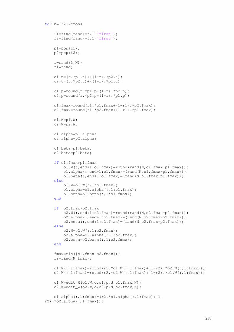
for n=1:2:Ncross i1=find(rand<=f,1,'first'); i2=find(rand<=f,1,'first'); p1=pop(i1); p2=pop(i2); r=rand(1,N); r1=rand; o1.t=(r.*p1.t)+((1-r).*p2.t); o2.t=(r.*p2.t)+((1-r).*p1.t); o1.p=round(r.*p1.p+(1-r).*p2.p); o2.p=round(r.*p2.p+(1-r).*p1.p); o1.fmax=round(r1.*p1.fmax+(1-r1).*p2.fmax); o2.fmax=round(r1.*p2.fmax+(1-r1).*p1.fmax); o1.W=p1.W; o2.W=p2.W; o1.alpha=p1.alpha; o2.alpha=p2.alpha; o1.beta=p1.beta; o2.beta=p2.beta; if o1.fmax>p1.fmax o1.W(:,end+1:o1.fmax)=round(rand(N,o1.fmax-p1.fmax)); o1.alpha(:,end+1:o1.fmax)=(rand(N,o1.fmax-p1.fmax)); o1.beta(:,end+1:o1.fmax)=(rand(N,o1.fmax-p1.fmax)); else o1.W=o1.W(:,1:o1.fmax); o1.alpha=o1.alpha(:,1:o1.fmax); o1.beta=o1.beta(:,1:o1.fmax); end if o2.fmax>p2.fmax o2.W(:,end+1:o2.fmax)=round(rand(N,o2.fmax-p2.fmax)); o2.alpha(:,end+1:o2.fmax)=(rand(N,o2.fmax-p2.fmax)); o2.beta(:,end+1:o2.fmax)=(rand(N,o2.fmax-p2.fmax)); else o2.W=o2.W(:,1:o2.fmax); o2.alpha=o2.alpha(:,1:o2.fmax); o2.beta=o2.beta(:,1:o2.fmax); end fmax=min([o1.fmax,o2.fmax]); r2=rand(N,fmax); o1.W(:,1:fmax)=round(r2.*o1.W(:,1:fmax)+(1-r2).*o2.W(:,1:fmax)); o2.W(:,1:fmax)=round(r2.*o2.W(:,1:fmax)+(1-r2).*o1.W(:,1:fmax)); o1.W=edit_W(o1.W,o,o1.p,d,o1.fmax,N); o2.W=edit_W(o2.W,o,o2.p,d,o2.fmax,N); o1.alpha(:,1:fmax)=(r2.*o1.alpha(:,1:fmax)+(1-r2).*o2.alpha(:,1:fmax));
238
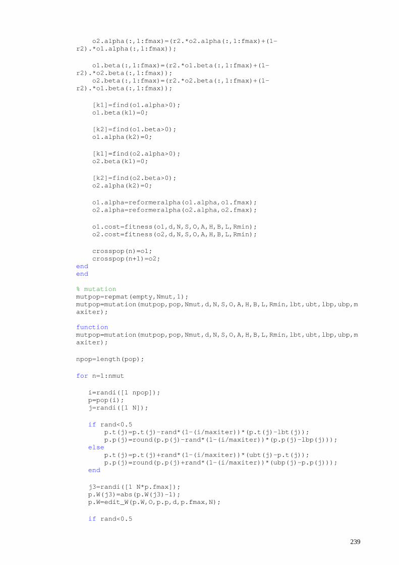
o2.alpha(:,1:fmax)=(r2.*o2.alpha(:,1:fmax)+(1-r2).*o1.alpha(:,1:fmax)); o1.beta(:,1:fmax)=(r2.*o1.beta(:,1:fmax)+(1-r2).*o2.beta(:,1:fmax)); o2.beta(:,1:fmax)=(r2.*o2.beta(:,1:fmax)+(1-r2).*o1.beta(:,1:fmax)); [k1]=find(o1.alpha>0); o1.beta(k1)=0; [k2]=find(o1.beta>0); o1.alpha(k2)=0; [k1]=find(o2.alpha>0); o2.beta(k1)=0; [k2]=find(o2.beta>0); o2.alpha(k2)=0; o1.alpha=reformeralpha(o1.alpha,o1.fmax); o2.alpha=reformeralpha(o2.alpha,o2.fmax); o1.cost=fitness(o1,d,N,S,O,A,H,B,L,Rmin); o2.cost=fitness(o2,d,N,S,O,A,H,B,L,Rmin); crosspop(n)=o1; crosspop(n+1)=o2; end end % mutation mutpop=repmat(empty,Nmut,1); mutpop=mutation(mutpop,pop,Nmut,d,N,S,O,A,H,B,L,Rmin,lbt,ubt,lbp,ubp,maxiter); function mutpop=mutation(mutpop,pop,Nmut,d,N,S,O,A,H,B,L,Rmin,lbt,ubt,lbp,ubp,maxiter); npop=length(pop); for n=1:nmut i=randi([1 npop]); p=pop(i); j=randi([1 N]); if rand<0.5 p.t(j)=p.t(j)-rand*(1-(i/maxiter))*(p.t(j)-lbt(j)); p.p(j)=round(p.p(j)-rand*(1-(i/maxiter))*(p.p(j)-lbp(j))); else p.t(j)=p.t(j)+rand*(1-(i/maxiter))*(ubt(j)-p.t(j)); p.p(j)=round(p.p(j)+rand*(1-(i/maxiter))*(ubp(j)-p.p(j))); end j3=randi([1 N*p.fmax]); p.W(j3)=abs(p.W(j3)-1); p.W=edit_W(p.W,O,p.p,d,p.fmax,N); if rand<0.5
239
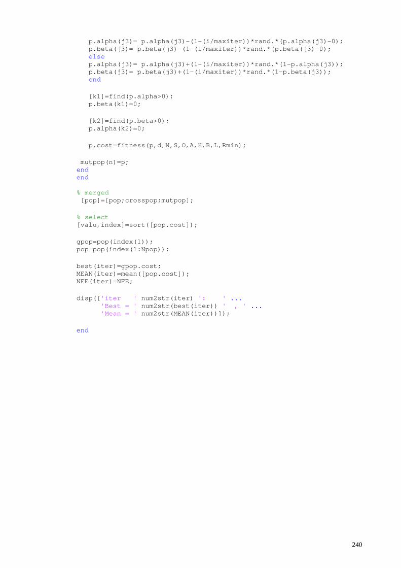
p.alpha(j3)= p.alpha(j3)-(1-(i/maxiter))*rand.*(p.alpha(j3)-0); p.beta(j3)= p.beta(j3)-(1-(i/maxiter))*rand.*(p.beta(j3)-0); else p.alpha(j3)= p.alpha(j3)+(1-(i/maxiter))*rand.*(1-p.alpha(j3)); p.beta(j3)= p.beta(j3)+(1-(i/maxiter))*rand.*(1-p.beta(j3)); end [k1]=find(p.alpha>0); p.beta(k1)=0; [k2]=find(p.beta>0); p.alpha(k2)=0; p.cost=fitness(p,d,N,S,O,A,H,B,L,Rmin); mutpop(n)=p; end end % merged [pop]=[pop;crosspop;mutpop]; % select [valu,index]=sort([pop.cost]); gpop=pop(index(1)); pop=pop(index(1:Npop)); best(iter)=gpop.cost; MEAN(iter)=mean([pop.cost]); NFE(iter)=NFE; disp(['iter ' num2str(iter) ': ' ... 'Best = ' num2str(best(iter)) ' , ' ... 'Mean = ' num2str(MEAN(iter))]); end
240
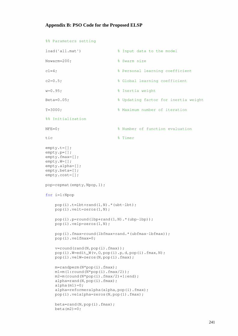
Appendix B: PSO Code for the Proposed ELSP
%% Parameters setting load('all.mat') % Input data to the model Nswarm=200; % Swarm size c1=4; % Personal learning coefficient c2=0.5; % Global learning coefficient w=0.95; % Inertia weight Beta=0.05; % Updating factor for inertia weight T=3000; % Maximum number of iteration %% Initialization NFE=0; % Number of function evaluation tic % Timer empty.t=[]; empty.p=[]; empty.fmax=[]; empty.W=[]; empty.alpha=[]; empty.beta=[]; empty.cost=[]; pop=repmat(empty,Npop,1); for i=1:Npop pop(i).t=lbt+rand(1,N).*(ubt-lbt); pop(i).velt=zeros(1,N); pop(i).p=round(lbp+rand(1,N).*(ubp-lbp)); pop(i).velp=zeros(1,N); pop(i).fmax=round(lbfmax+rand.*(ubfmax-lbfmax)); pop(i).velfmax=0; v=round(rand(N,pop(i).fmax)); pop(i).W=edit_W(v,O,pop(i).p,d,pop(i).fmax,N); pop(i).velW=zeros(N,pop(i).fmax); m=randperm(N*pop(i).fmax); m1=m(1:round(N*pop(i).fmax/2)); m2=m(round(N*pop(i).fmax/2)+1:end); alpha=rand(N,pop(i).fmax); alpha(m1)=0; alpha=reformeralpha(alpha,pop(i).fmax); pop(i).velalpha=zeros(N,pop(i).fmax); beta=rand(N,pop(i).fmax); beta(m2)=0;
241
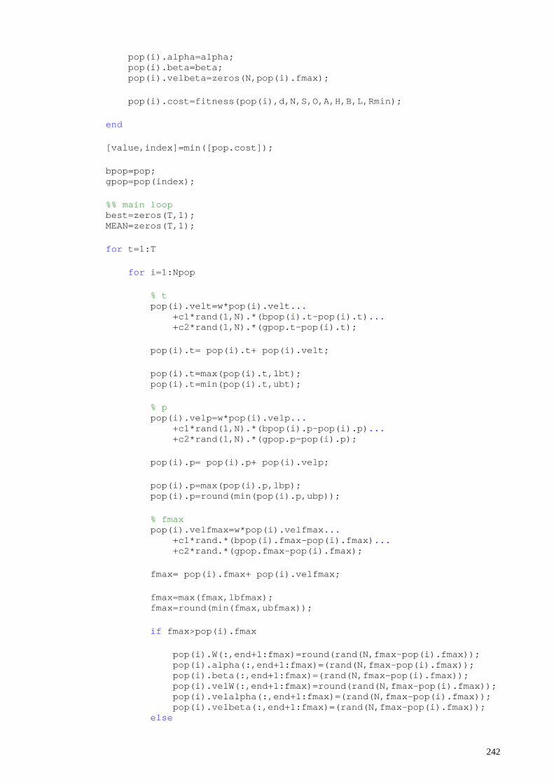
pop(i).alpha=alpha; pop(i).beta=beta; pop(i).velbeta=zeros(N,pop(i).fmax); pop(i).cost=fitness(pop(i),d,N,S,O,A,H,B,L,Rmin); end [value,index]=min([pop.cost]); bpop=pop; gpop=pop(index); %% main loop best=zeros(T,1); MEAN=zeros(T,1); for t=1:T for i=1:Npop % t pop(i).velt=w*pop(i).velt... +c1*rand(1,N).*(bpop(i).t-pop(i).t)... +c2*rand(1,N).*(gpop.t-pop(i).t); pop(i).t= pop(i).t+ pop(i).velt; pop(i).t=max(pop(i).t,lbt); pop(i).t=min(pop(i).t,ubt); % p pop(i).velp=w*pop(i).velp... +c1*rand(1,N).*(bpop(i).p-pop(i).p)... +c2*rand(1,N).*(gpop.p-pop(i).p); pop(i).p= pop(i).p+ pop(i).velp; pop(i).p=max(pop(i).p,lbp); pop(i).p=round(min(pop(i).p,ubp)); % fmax pop(i).velfmax=w*pop(i).velfmax... +c1*rand.*(bpop(i).fmax-pop(i).fmax)... +c2*rand.*(gpop.fmax-pop(i).fmax); fmax= pop(i).fmax+ pop(i).velfmax; fmax=max(fmax,lbfmax); fmax=round(min(fmax,ubfmax)); if fmax>pop(i).fmax pop(i).W(:,end+1:fmax)=round(rand(N,fmax-pop(i).fmax)); pop(i).alpha(:,end+1:fmax)=(rand(N,fmax-pop(i).fmax)); pop(i).beta(:,end+1:fmax)=(rand(N,fmax-pop(i).fmax)); pop(i).velW(:,end+1:fmax)=round(rand(N,fmax-pop(i).fmax)); pop(i).velalpha(:,end+1:fmax)=(rand(N,fmax-pop(i).fmax)); pop(i).velbeta(:,end+1:fmax)=(rand(N,fmax-pop(i).fmax)); else
242
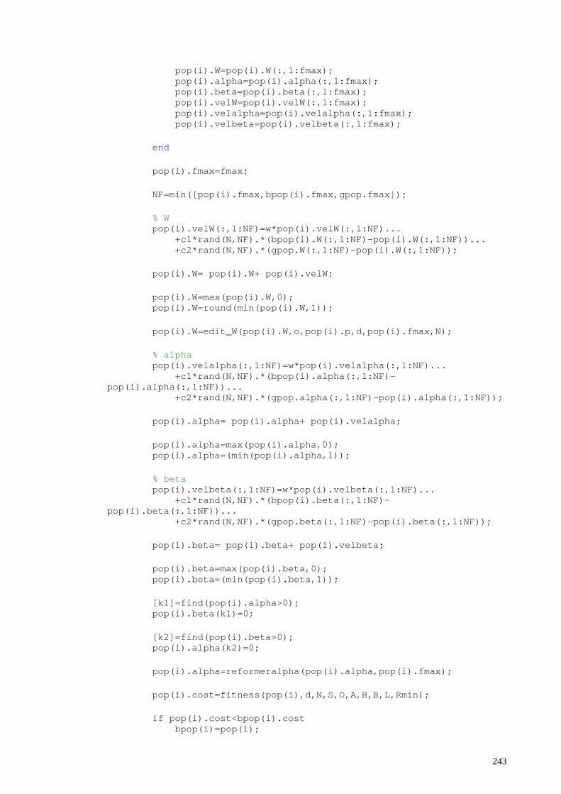
pop(i).W=pop(i).W(:,1:fmax); pop(i).alpha=pop(i).alpha(:,1:fmax); pop(i).beta=pop(i).beta(:,1:fmax); pop(i).velW=pop(i).velW(:,1:fmax); pop(i).velalpha=pop(i).velalpha(:,1:fmax); pop(i).velbeta=pop(i).velbeta(:,1:fmax); end pop(i).fmax=fmax; NF=min([pop(i).fmax,bpop(i).fmax,gpop.fmax]); % W pop(i).velW(:,1:NF)=w*pop(i).velW(:,1:NF)... +c1*rand(N,NF).*(bpop(i).W(:,1:NF)-pop(i).W(:,1:NF))... +c2*rand(N,NF).*(gpop.W(:,1:NF)-pop(i).W(:,1:NF)); pop(i).W= pop(i).W+ pop(i).velW; pop(i).W=max(pop(i).W,0); pop(i).W=round(min(pop(i).W,1)); pop(i).W=edit_W(pop(i).W,o,pop(i).p,d,pop(i).fmax,N); % alpha pop(i).velalpha(:,1:NF)=w*pop(i).velalpha(:,1:NF)... +c1*rand(N,NF).*(bpop(i).alpha(:,1:NF)-pop(i).alpha(:,1:NF))... +c2*rand(N,NF).*(gpop.alpha(:,1:NF)-pop(i).alpha(:,1:NF)); pop(i).alpha= pop(i).alpha+ pop(i).velalpha; pop(i).alpha=max(pop(i).alpha,0); pop(i).alpha=(min(pop(i).alpha,1)); % beta pop(i).velbeta(:,1:NF)=w*pop(i).velbeta(:,1:NF)... +c1*rand(N,NF).*(bpop(i).beta(:,1:NF)-pop(i).beta(:,1:NF))... +c2*rand(N,NF).*(gpop.beta(:,1:NF)-pop(i).beta(:,1:NF)); pop(i).beta= pop(i).beta+ pop(i).velbeta; pop(i).beta=max(pop(i).beta,0); pop(i).beta=(min(pop(i).beta,1)); [k1]=find(pop(i).alpha>0); pop(i).beta(k1)=0; [k2]=find(pop(i).beta>0); pop(i).alpha(k2)=0; pop(i).alpha=reformeralpha(pop(i).alpha,pop(i).fmax); pop(i).cost=fitness(pop(i),d,N,S,O,A,H,B,L,Rmin); if pop(i).cost<bpop(i).cost bpop(i)=pop(i);
243

if bpop(i).cost<gpop.cost gpop=bpop(i); end end end best(t)=gpop.cost; MEAN(t)=mean([bpop.cost]); w=w*(1-Beta); disp([' iter ' num2str(iter) ': ' ... ' Best = ' num2str(best(iter)) ' , ' ... ' Mean = ' num2str(MEAN(iter))]); end
244
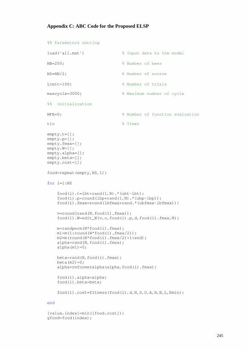
Appendix C: ABC Code for the Proposed ELSP
%% Parameters setting load('all.mat') % Input data to the model NB=200; % Number of bees NS=NB/2; % Number of source Limit=100; % Number of trials maxcycle=3000; % Maximum number of cycle %% Initialization NFE=0; % Number of function evaluation tic % Timer empty.t=[]; empty.p=[]; empty.fmax=[]; empty.W=[]; empty.alpha=[]; empty.beta=[]; empty.cost=[]; food=repmat(empty,NS,1); for i=1:NS food(i).t=lbt+rand(1,N).*(ubt-lbt); food(i).p=round(lbp+rand(1,N).*(ubp-lbp)); food(i).fmax=round(lbfmax+rand.*(ubfmax-lbfmax)); v=round(rand(N,food(i).fmax)); food(i).W=edit_W(v,o,food(i).p,d,food(i).fmax,N); m=randperm(N*food(i).fmax); m1=m(1:round(N*food(i).fmax/2)); m2=m(round(N*food(i).fmax/2)+1:end); alpha=rand(N,food(i).fmax); alpha(m1)=0; beta=rand(N,food(i).fmax); beta(m2)=0; alpha=reformeralpha(alpha,food(i).fmax); food(i).alpha=alpha; food(i).beta=beta; food(i).cost=fitness(food(i),d,N,S,O,A,H,B,L,Rmin); end [value,index]=min([food.cost]); gfood=food(index);
245
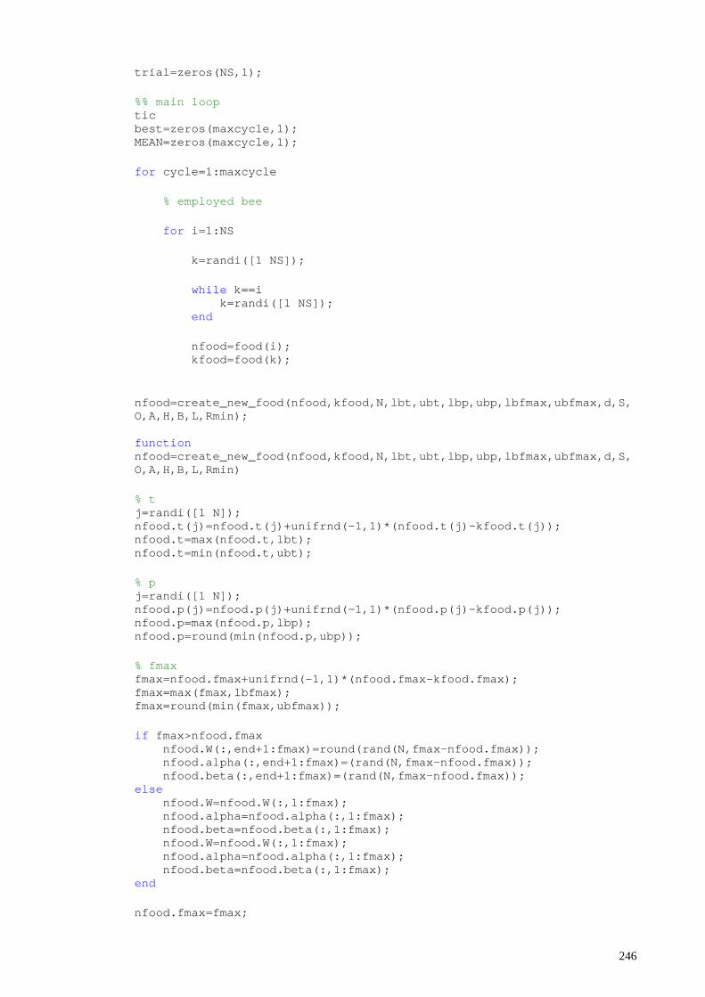
trial=zeros(NS,1); %% main loop tic best=zeros(maxcycle,1); MEAN=zeros(maxcycle,1); for cycle=1:maxcycle % employed bee for i=1:NS k=randi([1 NS]); while k==i k=randi([1 NS]); end nfood=food(i); kfood=food(k); nfood=create_new_food(nfood,kfood,N,lbt,ubt,lbp,ubp,lbfmax,ubfmax,d,S,O,A,H,B,L,Rmin); function nfood=create_new_food(nfood,kfood,N,lbt,ubt,lbp,ubp,lbfmax,ubfmax,d,S,O,A,H,B,L,Rmin) % t j=randi([1 N]); nfood.t(j)=nfood.t(j)+unifrnd(-1,1)*(nfood.t(j)-kfood.t(j)); nfood.t=max(nfood.t,lbt); nfood.t=min(nfood.t,ubt); % p j=randi([1 N]); nfood.p(j)=nfood.p(j)+unifrnd(-1,1)*(nfood.p(j)-kfood.p(j)); nfood.p=max(nfood.p,lbp); nfood.p=round(min(nfood.p,ubp)); % fmax fmax=nfood.fmax+unifrnd(-1,1)*(nfood.fmax-kfood.fmax); fmax=max(fmax,lbfmax); fmax=round(min(fmax,ubfmax)); if fmax>nfood.fmax nfood.W(:,end+1:fmax)=round(rand(N,fmax-nfood.fmax)); nfood.alpha(:,end+1:fmax)=(rand(N,fmax-nfood.fmax)); nfood.beta(:,end+1:fmax)=(rand(N,fmax-nfood.fmax)); else nfood.W=nfood.W(:,1:fmax); nfood.alpha=nfood.alpha(:,1:fmax); nfood.beta=nfood.beta(:,1:fmax); nfood.W=nfood.W(:,1:fmax); nfood.alpha=nfood.alpha(:,1:fmax); nfood.beta=nfood.beta(:,1:fmax); end nfood.fmax=fmax;
246
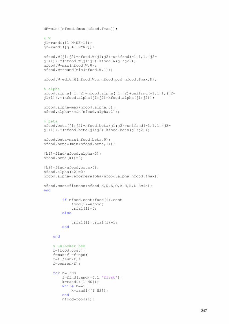
NF=min([nfood.fmax,kfood.fmax]); % W j1=randi([1 N*NF-1]); j2=randi([j1+1 N*NF]); nfood.W(j1:j2)=nfood.W(j1:j2)+unifrnd(-1,1,1,(j2-j1+1)).*(nfood.W(j1:j2)-kfood.W(j1:j2)); nfood.W=max(nfood.W,0); nfood.W=round(min(nfood.W,1)); nfood.W=edit_W(nfood.W,o,nfood.p,d,nfood.fmax,N); % alpha nfood.alpha(j1:j2)=nfood.alpha(j1:j2)+unifrnd(-1,1,1,(j2-j1+1)).*(nfood.alpha(j1:j2)-kfood.alpha(j1:j2)); nfood.alpha=max(nfood.alpha,0); nfood.alpha=(min(nfood.alpha,1)); % beta nfood.beta(j1:j2)=nfood.beta(j1:j2)+unifrnd(-1,1,1,(j2-j1+1)).*(nfood.beta(j1:j2)-kfood.beta(j1:j2)); nfood.beta=max(nfood.beta,0); nfood.beta=(min(nfood.beta,1)); [k1]=find(nfood.alpha>0); nfood.beta(k1)=0; [k2]=find(nfood.beta>0); nfood.alpha(k2)=0; nfood.alpha=reformeralpha(nfood.alpha,nfood.fmax); nfood.cost=fitness(nfood,d,N,S,O,A,H,B,L,Rmin); end if nfood.cost<food(i).cost food(i)=nfood; trial(i)=0; else trial(i)=trial(i)+1; end end % unlooker bee f=[food.cost]; f=max(f)-f+eps; f=f./sum(f); f=cumsum(f); for n=1:NS i=find(rand<=f,1,'first'); k=randi([1 NS]); while k==i k=randi([1 NS]); end nfood=food(i);
247
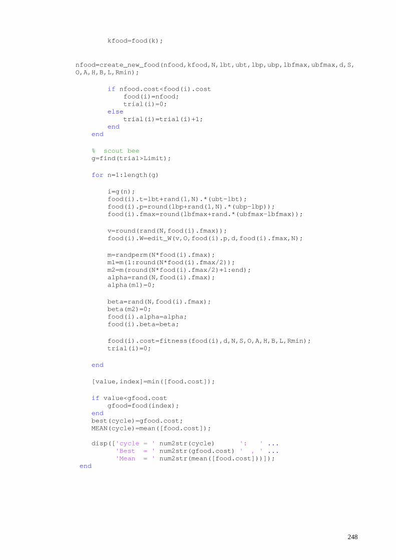
kfood=food(k); nfood=create_new_food(nfood,kfood,N,lbt,ubt,lbp,ubp,lbfmax,ubfmax,d,S,O,A,H,B,L,Rmin); if nfood.cost<food(i).cost food(i)=nfood; trial(i)=0; else trial(i)=trial(i)+1; end end % scout bee g=find(trial>Limit); for n=1:length(g) i=g(n); food(i).t=lbt+rand(1,N).*(ubt-lbt); food(i).p=round(lbp+rand(1,N).*(ubp-lbp)); food(i).fmax=round(lbfmax+rand.*(ubfmax-lbfmax)); v=round(rand(N,food(i).fmax)); food(i).W=edit_W(v,O,food(i).p,d,food(i).fmax,N); m=randperm(N*food(i).fmax); m1=m(1:round(N*food(i).fmax/2)); m2=m(round(N*food(i).fmax/2)+1:end); alpha=rand(N,food(i).fmax); alpha(m1)=0; beta=rand(N,food(i).fmax); beta(m2)=0; food(i).alpha=alpha; food(i).beta=beta; food(i).cost=fitness(food(i),d,N,S,O,A,H,B,L,Rmin); trial(i)=0; end [value,index]=min([food.cost]); if value<gfood.cost gfood=food(index); end best(cycle)=gfood.cost; MEAN(cycle)=mean([food.cost]); disp(['cycle = ' num2str(cycle) ': ' ... 'Best = ' num2str(gfood.cost) ' , ' ... 'Mean = ' num2str(mean([food.cost]))]); end
248
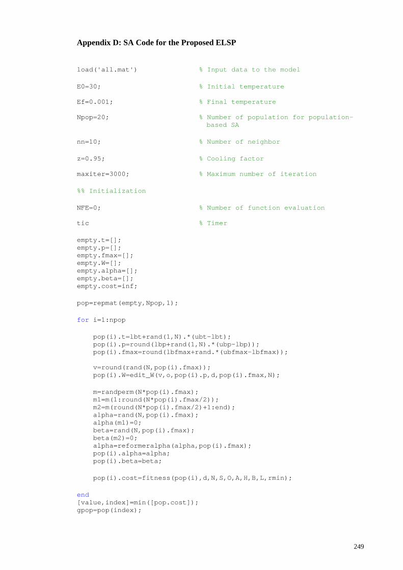
Appendix D: SA Code for the Proposed ELSP
load('all.mat') % Input data to the model E0=30; % Initial temperature Ef=0.001; % Final temperature Npop=20; % Number of population for population-
based SA nn=10; % Number of neighbor z=0.95; % Cooling factor maxiter=3000; % Maximum number of iteration %% Initialization NFE=0; % Number of function evaluation tic % Timer empty.t=[]; empty.p=[]; empty.fmax=[]; empty.W=[]; empty.alpha=[]; empty.beta=[]; empty.cost=inf; pop=repmat(empty,Npop,1); for i=1:npop pop(i).t=lbt+rand(1,N).*(ubt-lbt); pop(i).p=round(lbp+rand(1,N).*(ubp-lbp)); pop(i).fmax=round(lbfmax+rand.*(ubfmax-lbfmax)); v=round(rand(N,pop(i).fmax)); pop(i).W=edit_W(v,o,pop(i).p,d,pop(i).fmax,N); m=randperm(N*pop(i).fmax); m1=m(1:round(N*pop(i).fmax/2)); m2=m(round(N*pop(i).fmax/2)+1:end); alpha=rand(N,pop(i).fmax); alpha(m1)=0; beta=rand(N,pop(i).fmax); beta(m2)=0; alpha=reformeralpha(alpha,pop(i).fmax); pop(i).alpha=alpha; pop(i).beta=beta; pop(i).cost=fitness(pop(i),d,N,S,O,A,H,B,L,rmin); end [value,index]=min([pop.cost]); gpop=pop(index);
249
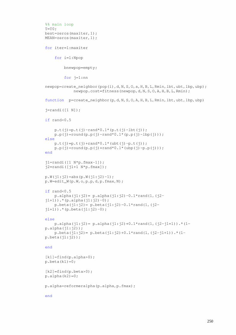
%% main loop T=T0; best=zeros(maxiter,1); MEAN=zeros(maxiter,1); for iter=1:maxiter for i=1:Npop bnewpop=empty; for j=1:nn newpop=create_neighbor(pop(i),d,N,S,O,a,H,B,L,Rmin,lbt,ubt,lbp,ubp); newpop.cost=fitness(newpop,d,N,S,O,A,H,B,L,Rmin); function p=create_neighbor(p,d,N,S,O,A,H,B,L,Rmin,lbt,ubt,lbp,ubp) j=randi([1 N]); if rand<0.5 p.t(j)=p.t(j)-rand*0.1*(p.t(j)-lbt(j)); p.p(j)=round(p.p(j)-rand*0.1*(p.p(j)-lbp(j))); else p.t(j)=p.t(j)+rand*0.1*(ubt(j)-p.t(j)); p.p(j)=round(p.p(j)+rand*0.1*(ubp(j)-p.p(j))); end j1=randi([1 N*p.fmax-1]); j2=randi([j1+1 N*p.fmax]); p.W(j1:j2)=abs(p.W(j1:j2)-1); p.W=edit_W(p.W,o,p.p,d,p.fmax,N); if rand<0.5 p.alpha(j1:j2)= p.alpha(j1:j2)-0.1*rand(1,(j2-j1+1)).*(p.alpha(j1:j2)-0); p.beta(j1:j2)= p.beta(j1:j2)-0.1*rand(1,(j2-j1+1)).*(p.beta(j1:j2)-0); else p.alpha(j1:j2)= p.alpha(j1:j2)+0.1*rand(1,(j2-j1+1)).*(1-p.alpha(j1:j2)); p.beta(j1:j2)= p.beta(j1:j2)+0.1*rand(1,(j2-j1+1)).*(1-p.beta(j1:j2)); end [k1]=find(p.alpha>0); p.beta(k1)=0; [k2]=find(p.beta>0); p.alpha(k2)=0; p.alpha=reformeralpha(p.alpha,p.fmax); end
250
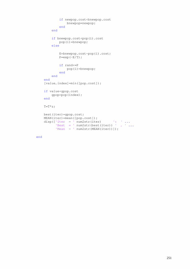
if newpop.cost<bnewpop.cost bnewpop=newpop; end end if bnewpop.cost<pop(i).cost pop(i)=bnewpop; else E=bnewpop.cost-pop(i).cost; P=exp(-E/T); if rand<=P pop(i)=bnewpop; end end end [value,index]=min([pop.cost]); if value<gpop.cost gpop=pop(index); end T=T*z; best(iter)=gpop.cost; MEAN(iter)=mean([pop.cost]); disp(['iter = ' num2str(iter) ': ' ... 'Best = ' num2str(best(iter)) ' , ' ... 'Mean = ' num2str(MEAN(iter))]); end
251
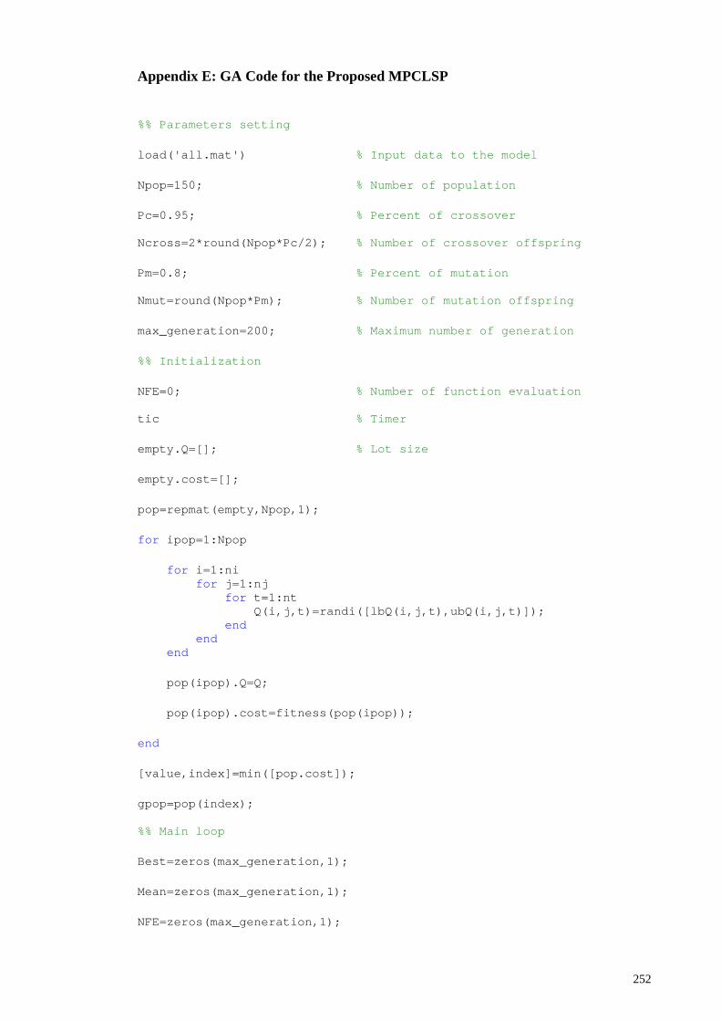
Appendix E: GA Code for the Proposed MPCLSP
%% Parameters setting load('all.mat') % Input data to the model Npop=150; % Number of population Pc=0.95; % Percent of crossover Ncross=2*round(Npop*Pc/2); % Number of crossover offspring Pm=0.8; % Percent of mutation Nmut=round(Npop*Pm); % Number of mutation offspring max_generation=200; % Maximum number of generation %% Initialization NFE=0; % Number of function evaluation tic % Timer empty.Q=[]; % Lot size empty.cost=[]; pop=repmat(empty,Npop,1); for ipop=1:Npop for i=1:ni for j=1:nj for t=1:nt Q(i,j,t)=randi([lbQ(i,j,t),ubQ(i,j,t)]); end end end pop(ipop).Q=Q; pop(ipop).cost=fitness(pop(ipop)); end [value,index]=min([pop.cost]); gpop=pop(index); %% Main loop Best=zeros(max_generation,1); Mean=zeros(max_generation,1); NFE=zeros(max_generation,1);
252
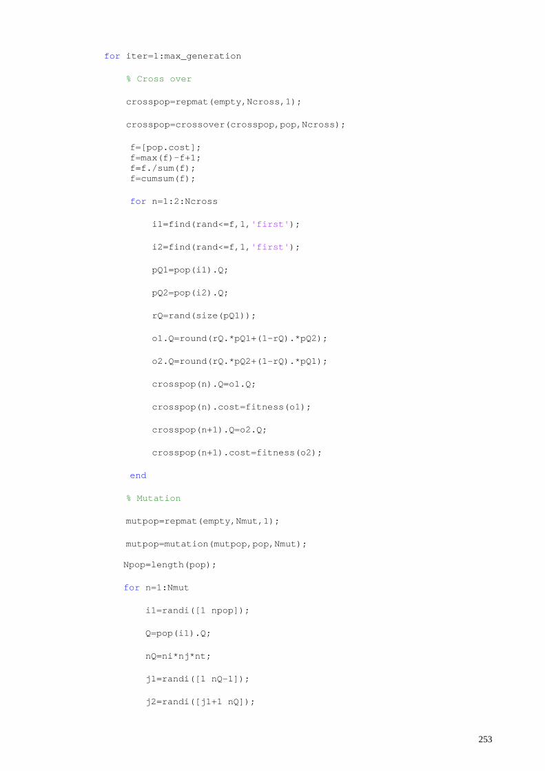
for iter=1:max_generation % Cross over crosspop=repmat(empty,Ncross,1); crosspop=crossover(crosspop,pop,Ncross);
f=[pop.cost]; f=max(f)-f+1; f=f./sum(f); f=cumsum(f); for n=1:2:Ncross i1=find(rand<=f,1,'first'); i2=find(rand<=f,1,'first'); pQ1=pop(i1).Q; pQ2=pop(i2).Q; rQ=rand(size(pQ1)); o1.Q=round(rQ.*pQ1+(1-rQ).*pQ2); o2.Q=round(rQ.*pQ2+(1-rQ).*pQ1); crosspop(n).Q=o1.Q; crosspop(n).cost=fitness(o1); crosspop(n+1).Q=o2.Q; crosspop(n+1).cost=fitness(o2); end
% Mutation mutpop=repmat(empty,Nmut,1); mutpop=mutation(mutpop,pop,Nmut);
Npop=length(pop); for n=1:Nmut i1=randi([1 npop]); Q=pop(i1).Q; nQ=ni*nj*nt; j1=randi([1 nQ-1]); j2=randi([j1+1 nQ]);
253
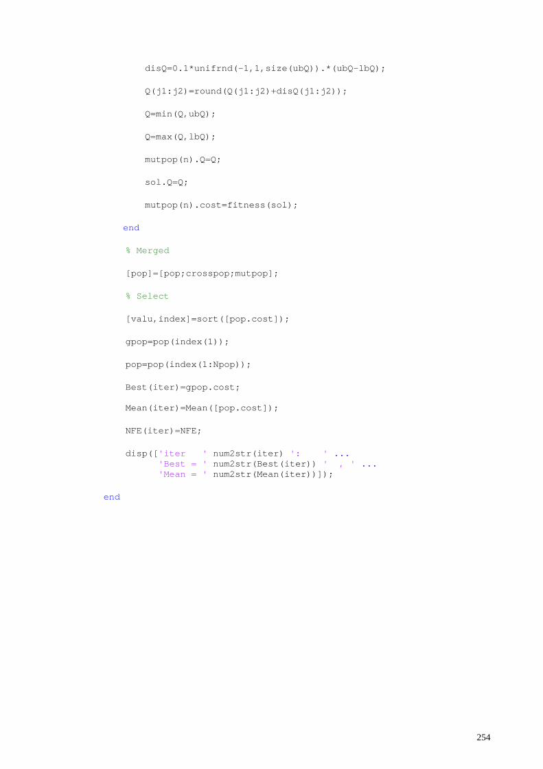
disQ=0.1*unifrnd(-1,1,size(ubQ)).*(ubQ-lbQ); Q(j1:j2)=round(Q(j1:j2)+disQ(j1:j2)); Q=min(Q,ubQ); Q=max(Q,lbQ); mutpop(n).Q=Q; sol.Q=Q; mutpop(n).cost=fitness(sol); end
% Merged [pop]=[pop;crosspop;mutpop]; % Select [valu,index]=sort([pop.cost]); gpop=pop(index(1)); pop=pop(index(1:Npop)); Best(iter)=gpop.cost; Mean(iter)=Mean([pop.cost]); NFE(iter)=NFE; disp(['iter ' num2str(iter) ': ' ... 'Best = ' num2str(Best(iter)) ' , ' ... 'Mean = ' num2str(Mean(iter))]); end
254
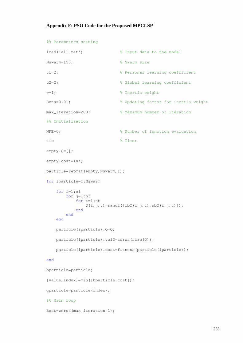
Appendix F: PSO Code for the Proposed MPCLSP
%% Parameters setting load('all.mat') % Input data to the model Nswarm=150; % Swarm size c1=2; % Personal learning coefficient c2=2; % Global learning coefficient w=1; % Inertia weight Beta=0.01; % Updating factor for inertia weight max_iteration=200; % Maximum number of iteration %% Initialization NFE=0; % Number of function evaluation tic % Timer empty.Q=[]; empty.cost=inf; particle=repmat(empty,Nswarm,1); for iparticle=1:Nswarm for i=1:ni for j=1:nj for t=1:nt Q(i,j,t)=randi([lbQ(i,j,t),ubQ(i,j,t)]); end end end particle(iparticle).Q=Q; particle(iparticle).velQ=zeros(size(Q)); particle(iparticle).cost=fitness(particle(iparticle)); end bparticle=particle; [value,index]=min([bparticle.cost]); gparticle=particle(index); %% Main loop Best=zeros(max_iteration,1);
255
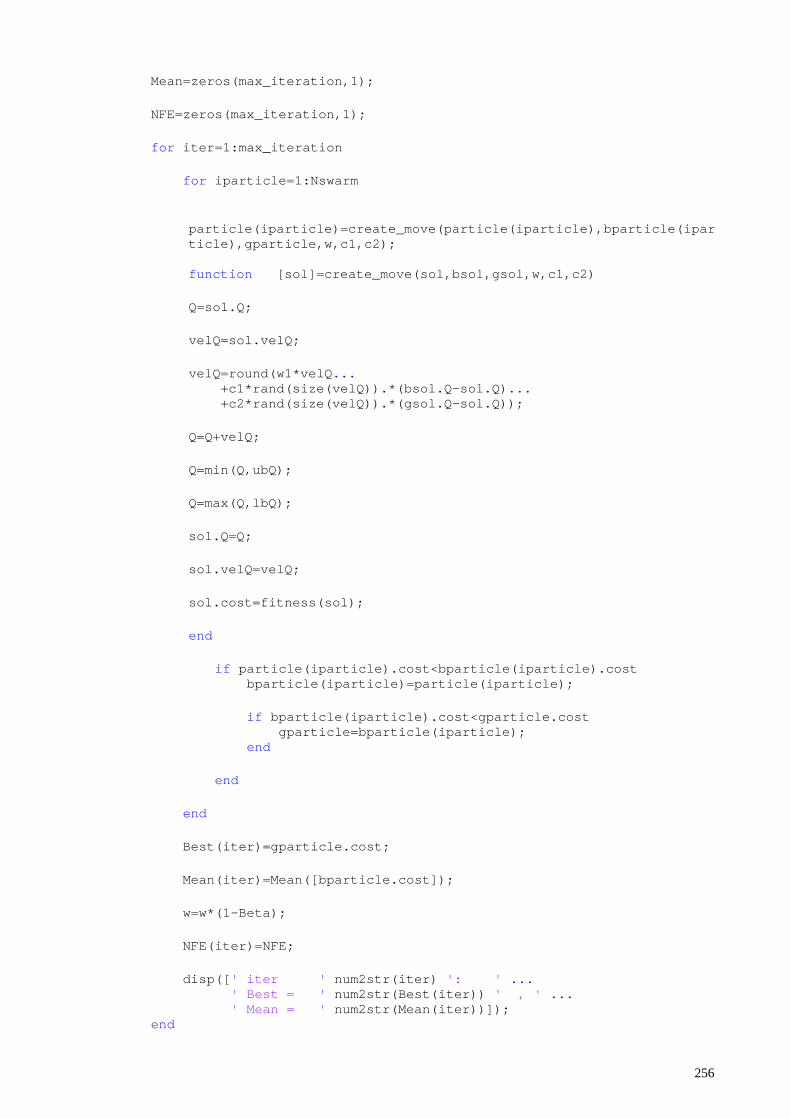
Mean=zeros(max_iteration,1); NFE=zeros(max_iteration,1); for iter=1:max_iteration for iparticle=1:Nswarm
particle(iparticle)=create_move(particle(iparticle),bparticle(iparticle),gparticle,w,c1,c2); function [sol]=create_move(sol,bsol,gsol,w,c1,c2) Q=sol.Q; velQ=sol.velQ; velQ=round(w1*velQ... +c1*rand(size(velQ)).*(bsol.Q-sol.Q)... +c2*rand(size(velQ)).*(gsol.Q-sol.Q)); Q=Q+velQ; Q=min(Q,ubQ); Q=max(Q,lbQ); sol.Q=Q; sol.velQ=velQ; sol.cost=fitness(sol); end
if particle(iparticle).cost<bparticle(iparticle).cost bparticle(iparticle)=particle(iparticle); if bparticle(iparticle).cost<gparticle.cost gparticle=bparticle(iparticle); end end end Best(iter)=gparticle.cost; Mean(iter)=Mean([bparticle.cost]); w=w*(1-Beta); NFE(iter)=NFE; disp([' iter ' num2str(iter) ': ' ... ' Best = ' num2str(Best(iter)) ' , ' ... ' Mean = ' num2str(Mean(iter))]); end
256
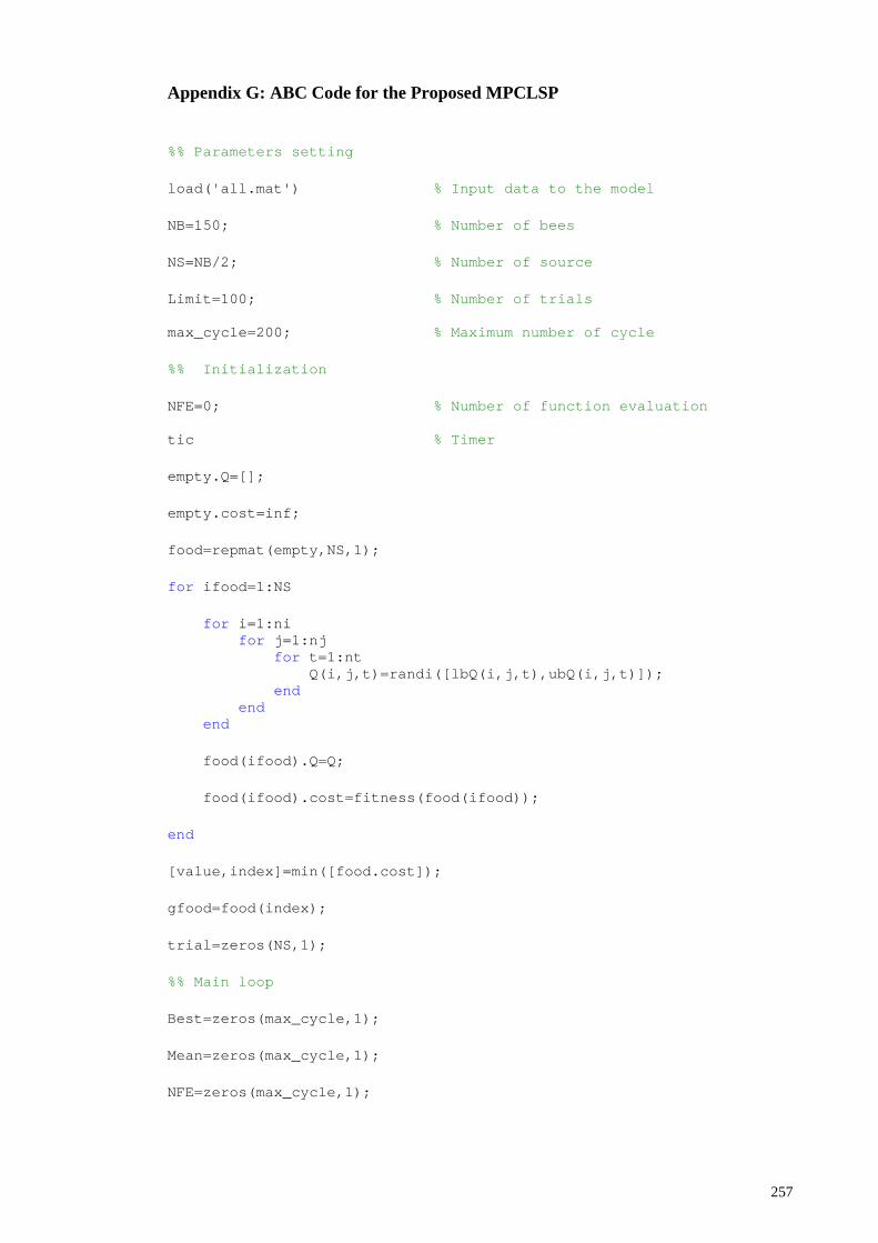
Appendix G: ABC Code for the Proposed MPCLSP
%% Parameters setting load('all.mat') % Input data to the model NB=150; % Number of bees NS=NB/2; % Number of source Limit=100; % Number of trials max_cycle=200; % Maximum number of cycle %% Initialization NFE=0; % Number of function evaluation tic % Timer empty.Q=[]; empty.cost=inf; food=repmat(empty,NS,1); for ifood=1:NS for i=1:ni for j=1:nj for t=1:nt Q(i,j,t)=randi([lbQ(i,j,t),ubQ(i,j,t)]); end end end food(ifood).Q=Q; food(ifood).cost=fitness(food(ifood)); end [value,index]=min([food.cost]); gfood=food(index); trial=zeros(NS,1); %% Main loop Best=zeros(max_cycle,1); Mean=zeros(max_cycle,1); NFE=zeros(max_cycle,1);
257
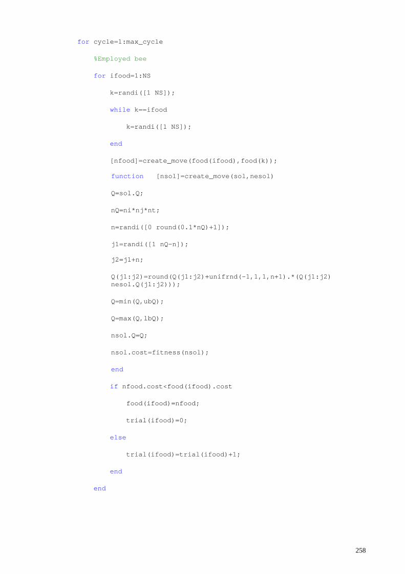
for cycle=1:max_cycle %Employed bee for ifood=1:NS k=randi([1 NS]); while k==ifood k=randi([1 NS]); end [nfood]=create_move(food(ifood),food(k));
function [nsol]=create_move(sol,nesol) Q=sol.Q; nQ=ni*nj*nt; n=randi([0 round(0.1*nQ)+1]); j1=randi([1 nQ-n]); j2=j1+n; Q(j1:j2)=round(Q(j1:j2)+unifrnd(-1,1,1,n+1).*(Q(j1:j2) nesol.Q(j1:j2))); Q=min(Q,ubQ); Q=max(Q,lbQ); nsol.Q=Q; nsol.cost=fitness(nsol); end
if nfood.cost<food(ifood).cost food(ifood)=nfood; trial(ifood)=0; else trial(ifood)=trial(ifood)+1; end end
258
%Unlooker bee f=[food.cost]; f=max(f)-f+eps; f=f./sum(f); f=cumsum(f); for n=1:NS ifood=find(rand<=f,1,'first'); k=randi([1 NS]); while k==ifood k=randi([1 NS]); end [nfood]=create_move(food(ifood),food(k)); if nfood.cost<food(ifood).cost food(ifood)=nfood; trial(ifood)=0; else trial(ifood)=trial(ifood)+1; end end %Scout bee g=find(trial>Limit); for n=1:length(g) ifood=g(n); for i=1:ni for j=1:nj for t=1:nt Q(i,j,t)=randi([lbQ(i,j,t),ubQ(i,j,t)]); end end end food(ifood).Q=Q; food(ifood).cost=fitness(food(ifood)); trial(ifood)=0; end
259
[value,index]=min([food.cost]); if value<gfood.cost gfood=food(index); end Best(cycle)=gfood.cost; Mean(cycle)=Mean([food.cost]); NFE(cycle)=NFE; disp(['cycle = ' num2str(cycle) ': ' ... 'Best = ' num2str(gfood.cost) ' , ' ... 'Mean = ' num2str(Mean([food.cost]))]); end
260
Appendix H: ICA Code for the Proposed MPCLSP
%% parameters setting load('all.mat') % Input data to the model Ncolony=150; % Number of colonies Nimp=10; % Number of imperialist Beta=2; % Assimilation coefficient Theta=0.3; % Revolution rate Gamma=0.25; % Coefficient for total cost of empire Max_decade=200; % Maximum number of decades %% Initialization NFE=0; % Number of function evaluation tic % Timer create_initial_imperialist empty.Q=[]; empty.cost=inf; colony=repmat(empty,Ncolony,1); for icolony=1:Ncolony for i=1:ni for j=1:nj for t=1:nt Q(i,j,t)=randi([lbQ(i,j,t),ubQ(i,j,t)]); %#ok end end end colony(icolony).Q=Q; colony(icolony).cost=fitness(colony(icolony)); end [value,index]=sort([colony.cost]); colony=colony(index); imp=colony(1:nimp); colony=colony(nimp+1:end); n=length(colony);
261
k=0; j=1; for i=1:n k=k+1; imp(k).colony(j)=colony(i); if k==nimp k=0; j=j+1; end end [value,index]=min([imp.cost]); gimp=imp(index); %% Main loop Best=zeros(max_decade,1); Mean=zeros(max_decade,1); NFE=zeros(max_decade,1); for decade=1:max_decade imp=assimulate(imp,Beta);
function imp=assimulate(imp,Beta) nimp=length(imp); for i=1:nimp Ncolony=length(imp(i).colony); for j=1:Ncolony
[imp(i).colony(j)]=create_move1(imp(i),imp(i).colony(j),Beta);
function [colony]=create_move1(imp,colony,Beta) dQ=imp.Q-colony.Q; dQ=round(beta*rand(size(dQ)).*dQ); colony.Q=colony.Q+dQ; colony.Q=min(colony.Q,ubQ); colony.Q=max(colony.Q,lbQ); colony.cost=fitness(colony); end
end end
262
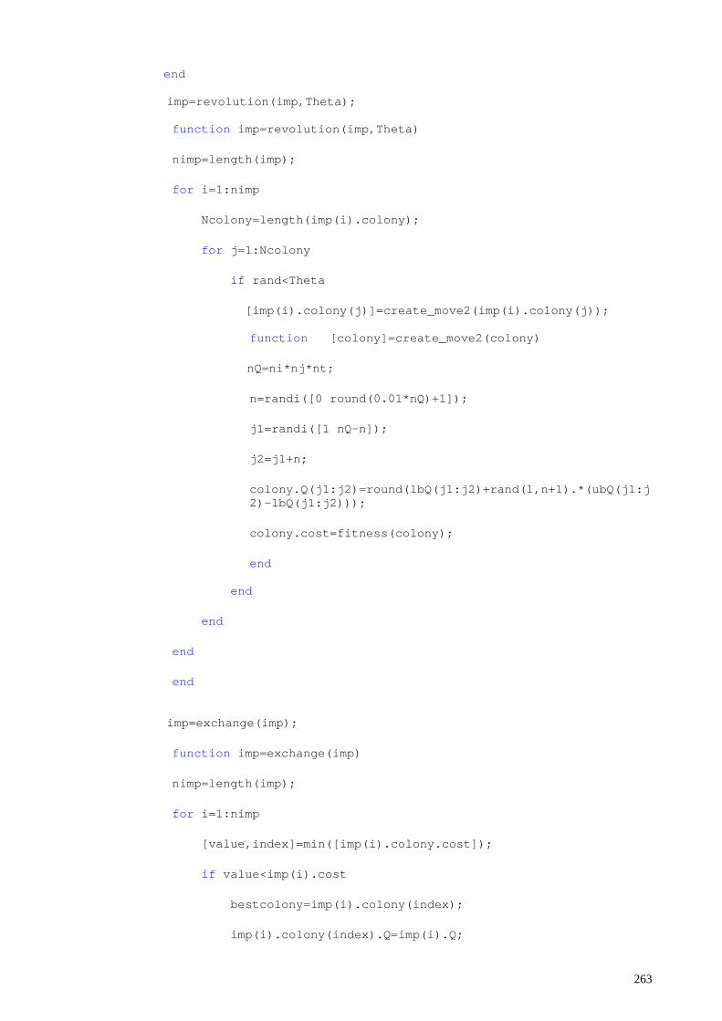
end
imp=revolution(imp,Theta);
function imp=revolution(imp,Theta) nimp=length(imp); for i=1:nimp Ncolony=length(imp(i).colony); for j=1:Ncolony if rand<Theta [imp(i).colony(j)]=create_move2(imp(i).colony(j));
function [colony]=create_move2(colony)
nQ=ni*nj*nt;
n=randi([0 round(0.01*nQ)+1]); j1=randi([1 nQ-n]); j2=j1+n; colony.Q(j1:j2)=round(lbQ(j1:j2)+rand(1,n+1).*(ubQ(j1:j2)-lbQ(j1:j2))); colony.cost=fitness(colony); end
end end end end
imp=exchange(imp);
function imp=exchange(imp) nimp=length(imp); for i=1:nimp [value,index]=min([imp(i).colony.cost]); if value<imp(i).cost bestcolony=imp(i).colony(index); imp(i).colony(index).Q=imp(i).Q;
263
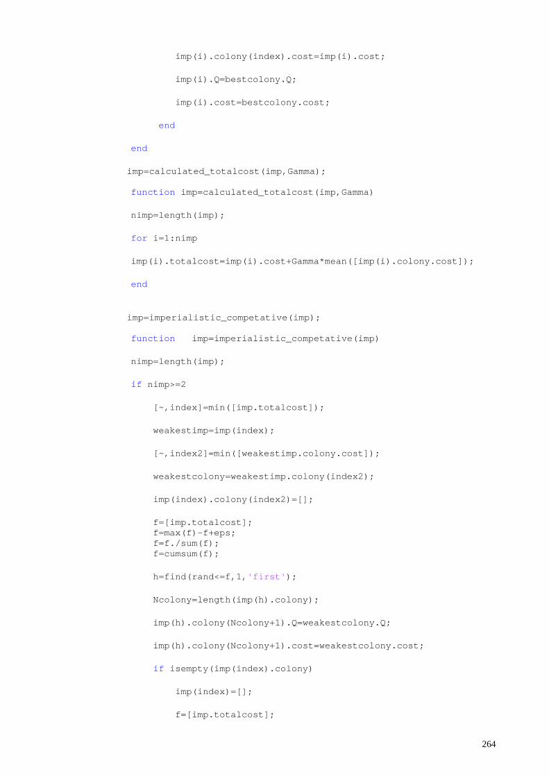
imp(i).colony(index).cost=imp(i).cost; imp(i).Q=bestcolony.Q; imp(i).cost=bestcolony.cost; end end
imp=calculated_totalcost(imp,Gamma);
function imp=calculated_totalcost(imp,Gamma) nimp=length(imp); for i=1:nimp imp(i).totalcost=imp(i).cost+Gamma*mean([imp(i).colony.cost]); end
imp=imperialistic_competative(imp);
function imp=imperialistic_competative(imp) nimp=length(imp); if nimp>=2 [~,index]=min([imp.totalcost]); weakestimp=imp(index); [~,index2]=min([weakestimp.colony.cost]); weakestcolony=weakestimp.colony(index2); imp(index).colony(index2)=[]; f=[imp.totalcost]; f=max(f)-f+eps; f=f./sum(f); f=cumsum(f); h=find(rand<=f,1,'first'); Ncolony=length(imp(h).colony); imp(h).colony(Ncolony+1).Q=weakestcolony.Q; imp(h).colony(Ncolony+1).cost=weakestcolony.cost; if isempty(imp(index).colony) imp(index)=[]; f=[imp.totalcost];
264
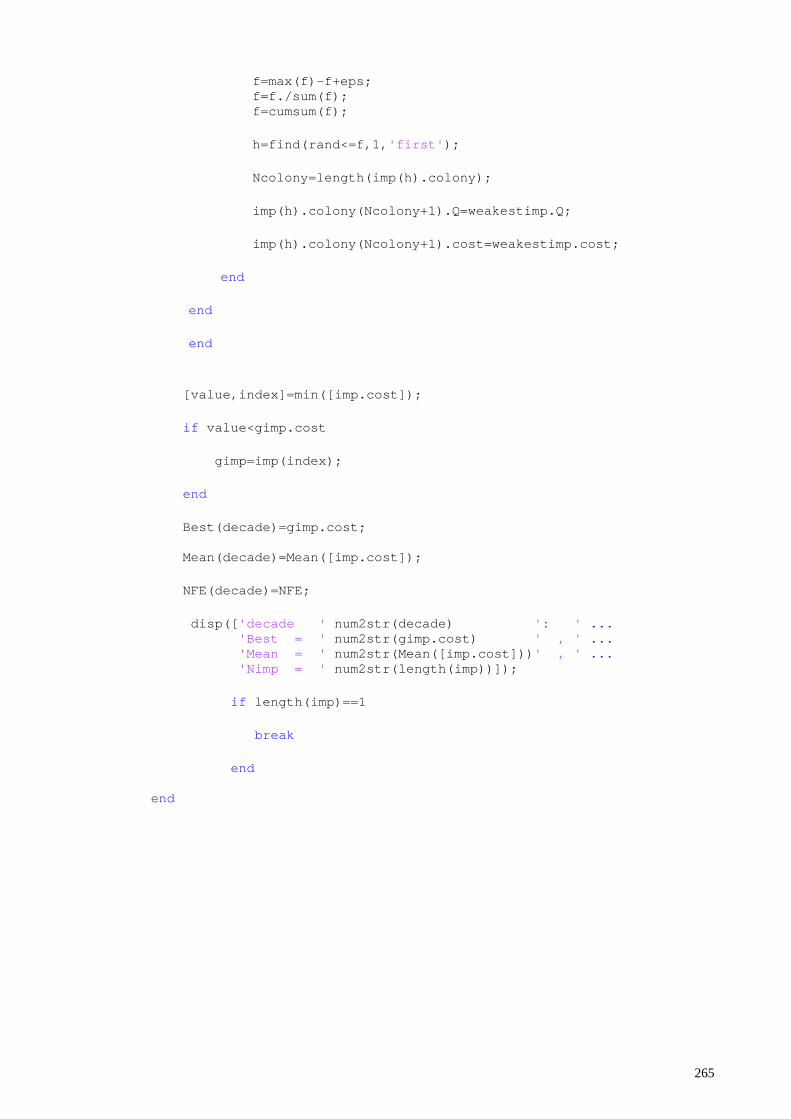
f=max(f)-f+eps; f=f./sum(f); f=cumsum(f); h=find(rand<=f,1,'first'); Ncolony=length(imp(h).colony); imp(h).colony(Ncolony+1).Q=weakestimp.Q; imp(h).colony(Ncolony+1).cost=weakestimp.cost; end end end
[value,index]=min([imp.cost]); if value<gimp.cost gimp=imp(index); end Best(decade)=gimp.cost; Mean(decade)=Mean([imp.cost]); NFE(decade)=NFE; disp(['decade ' num2str(decade) ': ' ... 'Best = ' num2str(gimp.cost) ' , ' ... 'Mean = ' num2str(Mean([imp.cost]))' , ' ... 'Nimp = ' num2str(length(imp))]); if length(imp)==1 break end end
265