Embed Size (px)
Citation preview

Brain Tumor Segmentation with Deep NeuralNetworks
Mohammad Havaei ∗1, Axel Davy †2, David Warde-Farley‡3, Antoine Biard§3,4,Aaron Courville¶3, Yoshua Bengio‖3, Chris Pal∗∗3,5, Pierre-Marc Jodoin††1, and
Hugo Larochelle‡‡1,6
1Université de Sherbrooke, Sherbrooke, Canada2École Normale supérieure, Paris, France
3Université de Montréal, Montréal, Canada4École polytechnique, Palaiseau, France
5École Polytechnique de Montréal , Canada6Twitter, USA
Abstract
In this paper, we present a fully automatic brain tumor segmenta-tion method based on Deep Neural Networks (DNNs). The proposednetworks are tailored to glioblastomas (both low and high grade) pic-tured in MR images. By their very nature, these tumors can appearanywhere in the brain and have almost any kind of shape, size, andcontrast. These reasons motivate our exploration of a machine learn-ing solution that exploits a flexible, high capacity DNN while beingextremely efficient. Here, we give a description of different modelchoices that we’ve found to be necessary for obtaining competitiveperformance. We explore in particular different architectures based on
∗[email protected]†[email protected]‡[email protected]§[email protected]¶[email protected]‖[email protected]∗∗[email protected]††[email protected]‡‡[email protected]
1
arX
iv:1
505.
0354
0v2
[cs
.CV
] 5
Oct
201
5

Convolutional Neural Networks (CNN), i.e. DNNs specifically adaptedto image data.
We present a novel CNN architecture which differs from those tra-ditionally used in computer vision. Our CNN exploits both local fea-tures as well as more global contextual features simultaneously. Also,different from most traditional uses of CNNs, our networks use a finallayer that is a convolutional implementation of a fully connected layerwhich allows a 40 fold speed up. We also describe a 2-phase trainingprocedure that allows us to tackle difficulties related to the imbalanceof tumor labels. Finally, we explore a cascade architecture in whichthe output of a basic CNN is treated as an additional source of infor-mation for a subsequent CNN. Results reported on the 2013 BRATStest dataset reveal that our architecture improves over the currentlypublished state-of-the-art while being over 30 times faster.
1 IntroductionIn the United States alone, it is estimated that 23,000 new cases of braincancer will be diagnosed in 20151. While gliomas are the most commonbrain tumors, they can be less aggressive (i.e. low grade) in a patient witha life expectancy of several years, or more aggressive (i.e. high grade) in apatient with a life expectancy of at most 2 years.
Although surgery is the most common treatment for brain tumors, ra-diation and chemotherapy may be used to slow the growth of tumors thatcannot be physically removed. Magnetic resonance imaging (MRI) providesdetailed images of the brain, and is one of the most common tests used todiagnose brain tumors. All the more, brain tumor segmentation from MR im-ages can have great impact for improved diagnostics, growth rate predictionand treatment planning.
While some tumors such as meningiomas can be easily segmented, otherslike gliomas and glioblastomas are much more difficult to localize. Thesetumors (together with their surrounding edema) are often diffused, poorlycontrasted, and extend tentacle-like structures that make them difficult tosegment. Another fundamental difficulty with segmenting brain tumors isthat they can appear anywhere in the brain, in almost any shape and size.Furthermore, unlike images derived from X-ray computed tomography (CT)
1cancer.org
2
scans, the scale of voxel values in MR images is not standardized. Dependingon the type of MR machine used (1.5, 3 or 7 tesla) and the acquisition pro-tocol (field of view value, voxel resolution, gradient strength, b0 value, etc.),the same tumorous cells may end up having drastically different grayscalevalues when pictured in different hospitals.
Healthy brains are typically made of 3 types of tissues: the white mat-ter, the gray matter, and the cerebrospinal fluid. The goal of brain tumorsegmentation is to detect the location and extension of the tumor regions,namely active tumorous tissue (vascularized or not), necrotic tissue, andedema (swelling near the tumor). This is done by identifying abnormal areaswhen compared to normal tissue. Since glioblastomas are infiltrative tumors,their borders are often fuzzy and hard to distinguish from healthy tissues.As a solution, more than one MRI modality is often employed, e.g. T1 (spin-lattice relaxation), T1-contrasted (T1C), T2 (spin-spin relaxation), protondensity (PD) contrast imaging, diffusion MRI (dMRI), and fluid attenuationinversion recovery (FLAIR) pulse sequences. The contrast between thesemodalities gives almost a unique signature to each tissue type.
Most automatic brain tumor segmentation methods use hand-designedfeatures [14, 31]. These methods implement a classical machine learningpipeline according to which features are first extracted and then given to aclassifier whose training procedure does not affect the nature of those fea-tures. An alternative approach for designing task-adapted feature represen-tations is to learn a hierarchy of increasingly complex features directly fromin-domain data. Deep neural networks have been shown to excel at learningsuch feature hierarchies [7]. In this work, we apply this approach to learn fea-ture hierarchies adapted specifically to the task of brain tumor segmentationthat combine information across MRI modalities.
Specifically, we investigate several choices for training Convolutional Neu-ral Networks (CNNs), which are Deep Neural Networks (DNNs) adapted toimage data. We report their advantages, disadvantages and performance us-ing well established metrics. Although CNNs first appeared over two decadesago [28], they have recently become a mainstay of the computer vision com-munity due to their record-shattering performance in the ImageNet Large-Scale Visual Recognition Challenge [26]. While CNNs have also been suc-cessfully applied to segmentation problems [1, 30, 20], most of the previouswork has focused on non-medical tasks and many involve architectures thatare not well suited to medical imagery or brain tumor segmentation in par-ticular. Our preliminary work on using convolutional neural networks for
3

brain tumor segmentation together with two other methods using CNNs waspresented in BRATS‘14 workshop. However, those results were incompleteand required more investigation (More on this in chapter 2).
In this paper, we propose a number of specific CNN architectures fortackling brain tumor segmentation. Our architectures exploit the most re-cent advances in CNN design and training techniques, such as Maxout [17]hidden units and Dropout [40] regularization. We also investigate severalarchitectures which take into account both the local shape of tumors as wellas their context.
One problem with many machine learning methods is that they performpixel classification without taking into account the local dependencies of la-bels (i.e. segmentation labels are conditionally independent given the inputimage). To account for this, one can employ structured output methods suchas conditional random fields (CRFs), for which inference can be computation-ally expensive. Alternatively, one can model label dependencies by consider-ing the pixel-wise probability estimates of an initial CNN as additional inputto certain layers of a second DNN, forming a cascaded architecture. Sinceconvolutions are efficient operations, this approach can be significantly fasterthan implementing a CRF.
We focus our experimental analysis on the fully-annotated MICCAI braintumor segmentation (BRATS) challenge 2013 dataset [14] using the well de-fined training and testing splits, thereby allowing us to compare directly andquantitatively to a wide variety of other methods.
Our contributions in this work are four fold:
1. We propose a fully automatic method with results currently rankedsecond on the BRATS 2013 scoreboard;
2. To segment a brain, our method takes between 25 seconds and 3 min-utes, which is one order of magnitude faster than most state-of-the-artmethods.
3. Our CNN implements a novel two-pathway architecture that learnsabout the local details of the brain as well as the larger context. Wealso propose a two-phase training procedure which we have found iscritical to deal with imbalanced label distributions. Details of thesecontributions are described in Sections 3.1.1 and 3.2.
4. We employ a novel cascaded architecture as an efficient and conceptu-ally clean alternative to popular structured output methods. Details
4

on those models are presented in Section 3.1.2.
2 Related workAs noted by Menze et al. [31], the number of publications devoted to auto-mated brain tumor segmentation has grown exponentially in the last severaldecades. This observation not only underlines the need for automatic braintumor segmentation tools, but also shows that research in that area is still awork in progress.
Brain tumor segmentation methods (especially those devoted to MRI)can be roughly divided in two categories: those based on generative modelsand those based on discriminative models [31, 5, 2].
Generative models rely heavily on domain-specific prior knowledge aboutthe appearance of both healthy and tumorous tissues. Tissue appearance ischallenging to characterize, and existing generative models usually identify atumor as being a shape or a signal which deviates from a normal (or average)brain [8]. Typically, these methods rely on anatomical models obtained afteraligning the 3D MR image on an atlas or a template computed from severalhealthy brains [11]. A typical generative model of MR brain images can befound in Prastawa et al. [36]. Given the ICBM brain atlas, the method alignsthe brain to the atlas and computes posterior probabilities of healthy tissues(white matter, gray matter and cerebrospinal fluid) . Tumorous regions arethen found by localizing voxels whose posterior probability is below a certainthreshold. A post-processing step is then applied to ensure good spatialregularity. Prastawa et al. [37] also register brain images onto an atlas inorder to get a probability map for abnormalities. An active contour is theninitialized on this map and iterated until the change in posterior probabilityis below a certain threshold. Many other active-contour methods along thesame lines have been proposed [24, 9, 35], all of which depend on left-rightbrain symmetry features and/or alignment-based features. Note that sincealigning a brain with a large tumor onto a template can be challenging,some methods perform registration and tumor segmentation at the sametime [27, 33].
Other approaches for brain tumor segmentation employ discriminativemodels. Unlike generative modeling approaches, these approaches exploitlittle prior knowledge on the brain’s anatomy and instead rely mostly on theextraction of [a large number of] low level image features, directly modeling
5

the relationship between these features and the label of a given voxel. Thesefeatures may be raw input pixels values [21, 19], local histograms [25? ] tex-ture features such as Gabor filterbanks [42, 41], or alignment-based featuressuch as inter-image gradient, region shape difference, and symmetry analy-sis [32]. Classical discriminative learning techniques such as SVMs [4, 39, 29]and decision forests [? ] have also been used. Results from the 2012, 2013and 2014 editions of the MICCAI-BRATS Challenge suggest that methodsrelying on random forests are among the most accurate [31, 18, 25].
One common aspect with discriminative models is their implementationof a conventional machine learning pipeline relying on hand-designed fea-tures. For these methods, the classifier is trained to separate healthy fromnon-heatlthy tissues assuming that the input features have a sufficiently highdiscriminative power since the behavior the classifier is independent from na-ture of those features. One difficulty with methods based on hand-designedfeatures is that they often require the computation of a large number offeatures in order to be accurate when used with many traditional machinelearning techniques. This can make them slow to compute and expensivememory-wise. More efficient techniques employ lower numbers of features,using dimensionality reduction or feature selection methods, but the reduc-tion in the number of features is often at the cost of reduced accuracy.
By their nature, many hand-engineered features exploit very generic edge-related information, with no specific adaptation to the domain of brain tu-mors. Ideally, one would like to have features that are composed and refinedinto higher-level, task-adapted representations. Recently, preliminary inves-tigations have shown that the use of deep CNNs for brain tumor segmentationmakes for a very promising approach (see the BRATS 2014 challenge work-shop papers of Davy et al. [10], Zikic et al. [46], Urban et al. [43]). All threemethods divide the 3D MR images into 2D [10, 46] or 3D patches [43] andtrain a CNN to predict its center pixel class. Urban et al. [43] as well asZikic et al. [46] implemented a fairly common CNN, consisting of a seriesof convolutional layers, a non-linear activation function between each layerand a softmax output layer. Our work here2 extends our preliminary resultspresented in Davy et al. [10] using a two-pathway architecture, which we usehere as a building block.
2 It is important to note that while we did participate in the BRATS 2014 challenge,we could not report complete and fair experiments for it at the time of submitting thismanuscript. See Section 5 for a discussion on this point.
6
In computer vision, CNN-based segmentation models have typically beenapplied to natural scene labeling. For these tasks, the inputs to the modelare the RGB channels of a patch from a color image. The work in Pinheiroand Collobert [34] uses a basic CNN to make predictions for each pixel andfurther improves the predictions by using them as extra information in theinput of a second CNN model. Other work [12] involves several distinct CNNsprocessing the image at different resolutions. The final per-pixel class predic-tion is made by integrating information learned from all CNNs. To producea smooth segmentation, these predictions are regularized using a more globalsuperpixel segmentation of the image. Like our work, other recent work hasexploited convolution operations in the final layer of a network to extendtraditional CNN architectures for semantic scene segmentation [30]. In themedical imaging domain in general there has been comparatively less workusing CNNs for segmentation. However, some notable recent work by Huangand Jain [22] has used CNNs to predict the boundaries of neural tissue inelectron microscopy images. Here we explore an approach with similaritiesto the various approaches discussed above, but in the context of brain tumorsegmentation.
3 Our Convolutional Neural Network ApproachSince the brains in the BRATS dataset lack resolution in the third dimension,we consider performing the segmentation slice by slice from the axial view.Thus, our model processes sequentially each 2D axial image (slice) whereeach pixel is associated with different image modalities namely; T1, T2, T1Cand FLAIR. Like most CNN-based segmentation models [34, 12], our methodpredicts the class of a pixel by processing the M ×M patch centered on thatpixel. The input X of our CNN model is thus an M ×M 2D patch withseveral modalities.
The main building block used to construct a CNN architecture is the con-volutional layer. Several layers can be stacked on top of each other forminga hierarchy of features. Each layer can be understood as extracting featuresfrom its preceding layer into the hierarchy to which it is connected. A singleconvolutional layer takes as input a stack of input planes and produces asoutput some number of output planes or feature maps. Each feature mapcan be thought of as a topologically arranged map of responses of a particu-lar spatially local non-linear feature extractor (the parameters of which are
7

max
Maxout, K = 2
convolution, N = 3
max pooling, p = 2
5x5 4x4
5x57x7
7x7
HsZs
Os
Os+1
X
X
X
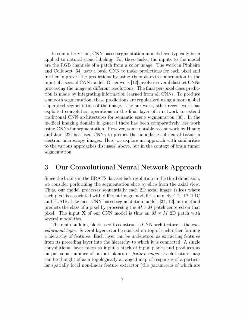
Figure 1: A single convolution layer block showing computations for a singlefeature map. The input patch (here 7×7), is convolved with series of kernels(here 3× 3) followed by Maxout and max-pooling.
learned), applied identically to each spatial neighborhood of the input planesin a sliding window fashion. In the case of a first convolutional layer, theindividual input planes correspond to different MRI modalities (in typicalcomputer vision applications, the individual input planes correspond to thered, green and blue color channels). In subsequent layers, the input planestypically consist of the feature maps of the previous layer.
Computing a feature map in a convolutional layer (see Figure 1 ) consistsof the following three steps:
1. Convolution of kernels (filters): Each feature mapOs is associated withone kernel (or several, in the case of Maxout). The feature map Os iscomputed as follows:
Os = bs +∑r
Wsr ∗Xr (1)
where Xr is the rth input channel, Wsr is the sub-kernel for that chan-nel, ∗ is the convolution operation and bs is a bias term3. In other
3Since the convolutional layer is associated to R input channels, X contains M×M×Rgray-scale values and thus each kernel Ws contains N ×N ×R weights. Accordingly, thenumber of parameters in a convolutional block of consisting of S feature maps is equal toR×M ×M × S.
8
words, the affine operation being performed for each feature map is thesum of the application of R different 2-dimensional N × N convolu-tion filters (one per input channel/modality), plus a bias term which isadded pixel-wise to each resulting spatial position. Though the inputto this operation is a M × M × R 3-dimensional tensor, the spatialtopology being considered is 2-dimensional in the X-Y axial plane ofthe original brain volume.
Whereas traditional image feature extraction methods rely on a fixedrecipe (sometimes taking the form of convolution with a linear e.g.Gabor filter bank), the key to the success of convolutional neural net-works is their ability to learn the weights and biases of individual fea-ture maps, giving rise to data-driven, customized, task-specific densefeature extractors. These parameters are adapted via stochastic gradi-ent descent on a surrogate loss function related to the misclassificationerror, with gradients computed efficiently via the backpropagation al-gorithm [38].
Special attention must be paid to the treatment of border pixels by theconvolution operation. Throughout our architecture, we employ theso-called valid-mode convolution, meaning that the filter response isnot computed for pixel positions that are less than bN/2c pixels awayfrom the image border. An N × N filter convolved with an M ×Minput patch will result in a Q×Q output, where Q = M −N + 1. InFigure 1, M = 7, N = 3 and thus Q = 5. Note that the size (spatialwidth and height) of the kernels are hyper-parameters that must bespecified by the user.
2. Non-linear activation function: To obtain features that are non-lineartransformations of the input, an element-wise non-linearity is appliedto the result of the kernel convolution. There are multiple choices forthis non-linearity, such as the sigmoid, hyperbolic tangent and rectifiedlinear functions [23], [15].
Recently, Goodfellow et al. [17] proposed a Maxout non-linearity, whichhas been shown to be particularly effective at modeling useful fea-tures. Maxout features are associated with multiple kernels Ws. Thisimplies each Maxout map Zs is associated with K feature maps :{Os,Os+1, ...,Os+K−1}. Note that in Figure 1, the Maxout maps areassociated with K = 2 feature maps. Maxout features correspond to
9

taking the max over the feature maps O, individually for each spatialposition:
Zs,i,j = max {Os,i,j, Os+1,i,j, ..., Os+K−1,i,j} (2)
where i, j are spatial positions. Maxout features are thus equivalent tousing a convex activation function, but whose shape is adaptive anddepends on the values taken by the kernels.
3. Max pooling: This operation consists of taking the maximum feature(neuron) value over sub-windows within each feature map. This can beformalized as follows:
Hs,i,j = maxpZs,i+p,j+p, (3)
where p determines the max pooling window size. The sub-windows canbe overlapping or not (Figure 1 shows an overlapping configuration).The max-pooling operation shrinks the size of the feature map. This iscontrolled by the pooling size p and the stride hyper-parameter, whichcorresponds to the horizontal and vertical increments at which poolingsub-windows are positioned. Let S be the stride value and Q×Q be theshape of the feature map before max-pooling. The output of the max-pooling operation would be of size D ×D, where D = (Q− p)/S + 1.In Figure 1, since Q = 5, p = 2, S = 1, the max-pooling operationresults into a D = 4 output feature map. The motivation for this oper-ation is to introduce invariance to local translations. This subsamplingprocedure has been found beneficial in other applications [26].
Convolutional networks have the ability to extract a hierarchy of increas-ingly complex features which makes them very appealing. This is done bytreating the output feature maps of a convolutional layer as input channelsto the subsequent convolutional layer.
From the neural network perspective, feature maps correspond to a layerof hidden units or neurons. Specifically, each coordinate within a feature mapcorresponds to an individual neuron, for which the size of its receptive fieldcorresponds to the kernel’s size. A kernel’s value also represents the weights ofthe connections between the layer’s neurons and the neurons in the previouslayer. It is often found in practice that the learned kernels resemble edge
10
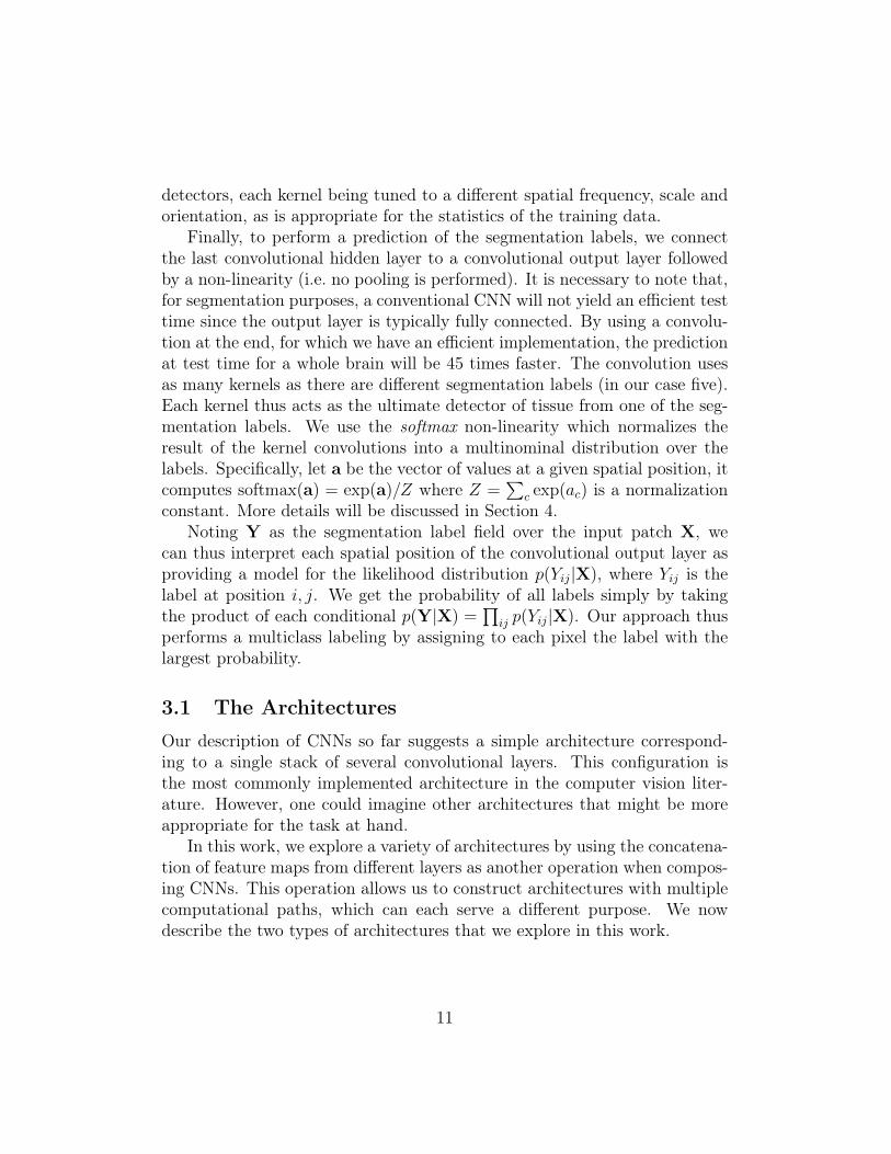
detectors, each kernel being tuned to a different spatial frequency, scale andorientation, as is appropriate for the statistics of the training data.
Finally, to perform a prediction of the segmentation labels, we connectthe last convolutional hidden layer to a convolutional output layer followedby a non-linearity (i.e. no pooling is performed). It is necessary to note that,for segmentation purposes, a conventional CNN will not yield an efficient testtime since the output layer is typically fully connected. By using a convolu-tion at the end, for which we have an efficient implementation, the predictionat test time for a whole brain will be 45 times faster. The convolution usesas many kernels as there are different segmentation labels (in our case five).Each kernel thus acts as the ultimate detector of tissue from one of the seg-mentation labels. We use the softmax non-linearity which normalizes theresult of the kernel convolutions into a multinominal distribution over thelabels. Specifically, let a be the vector of values at a given spatial position, itcomputes softmax(a) = exp(a)/Z where Z =
∑c exp(ac) is a normalization
constant. More details will be discussed in Section 4.Noting Y as the segmentation label field over the input patch X, we
can thus interpret each spatial position of the convolutional output layer asproviding a model for the likelihood distribution p(Yij|X), where Yij is thelabel at position i, j. We get the probability of all labels simply by takingthe product of each conditional p(Y|X) =
∏ij p(Yij|X). Our approach thus
performs a multiclass labeling by assigning to each pixel the label with thelargest probability.
3.1 The Architectures
Our description of CNNs so far suggests a simple architecture correspond-ing to a single stack of several convolutional layers. This configuration isthe most commonly implemented architecture in the computer vision liter-ature. However, one could imagine other architectures that might be moreappropriate for the task at hand.
In this work, we explore a variety of architectures by using the concatena-tion of feature maps from different layers as another operation when compos-ing CNNs. This operation allows us to construct architectures with multiplecomputational paths, which can each serve a different purpose. We nowdescribe the two types of architectures that we explore in this work.
11

Conv 3x3 +Maxout + Pooling 2x2
Conv 7x7 +Maxout + Pooling 4x4
Conv 13x13 +Maxout
Input4x33x33
Concatenation
Conv 21x21 +Softmax
Output5x1x1
64x21x2164x24x24
160x21x21
224x21x21
# Parameters 651,488
Figure 2: Two-pathway CNN architecture (TwoPathCNN). The figureshows the input patch going through two paths of convolutional operations.The feature-maps in the local and global paths are shown in yellow andorange respectively. The convolutional layers used to produce these feature-maps are indicated by dashed lines in the figure. The green box embodiesthe whole model which in later architectures will be used to indicate theTwoPathCNN.
3.1.1 Two-pathway architecture
This architecture is made of two streams: a pathway with smaller 7 × 7receptive fields and another with larger 13× 13 receptive fields. We refer tothese streams as the local pathway and the global pathway, respectively. Themotivation for this architectural choice is that we would like the predictionof the label of a pixel to be influenced by two aspects: the visual details ofthe region around that pixel and its larger “context", i.e. roughly where thepatch is in the brain.
The full architecture along with its details is illustrated in Figure 2. Werefer to this architecture as the TwoPathCNN. To allow for the concate-nation of the top hidden layers of both pathways, we use two layers for thelocal pathway, with 3 × 3 kernels for the second layer. While this impliesthat the effective receptive field of features in the top layer of each pathwayis the same, the global pathway’s parametrization more directly and flexiblymodels features in that same area. The concatenation of the feature maps ofboth pathways is then fed to the output layer.
3.1.2 Cascaded architectures
One disadvantage of the CNNs described so far is that they predict eachsegmentation label separately from each other. This is unlike a large numberof segmentation methods in the literature, which often propose a joint model
12
of the segmentation labels, effectively modeling the direct dependencies be-tween spatially close labels. One approach is to define a conditional randomfield (CRF) over the labels and perform mean-field message passing inferenceto produce a complete segmentation. In this case, the final label at a givenposition is effectively influenced by the models beliefs about what the labelis in the vicinity of that position.
On the other hand, inference in such joint segmentation methods is typi-cally more computationally expensive than a simple feed-forward pass througha CNN. This is an important aspect that one should take into account if au-tomatic brain tumor segmentation is to be used in a day-to-day practice.
Here, we describe CNN architectures that both exploit the efficiency ofCNNs, while also more directly model the dependencies between adjacentlabels in the segmentation. The idea is simple: since we’d like the ultimateprediction to be influenced by the model’s beliefs about the value of nearbylabels, we propose to feed the output probabilities of a first CNN as additionalinputs to the layers of a second CNN. Again, we do this by relying on theconcatenation of convolutional layers. In this case, we simply concatenatethe output layer of the first CNN with any of the layers in the second CNN.Moreover, we use the same two-pathway structure for both CNNs. Thiseffectively corresponds to a cascade of two CNNs, thus we refer to suchmodels as cascaded architectures.
In this work, we investigated three cascaded architectures that concate-nate the first CNN’s output at different levels of the second CNN:
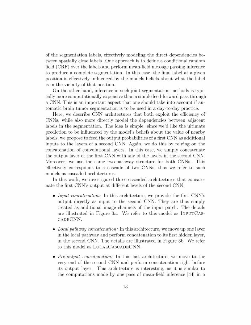
• Input concatenation: In this architecture, we provide the first CNN’soutput directly as input to the second CNN. They are thus simplytreated as additional image channels of the input patch. The detailsare illustrated in Figure 3a. We refer to this model as InputCas-cadeCNN.
• Local pathway concatenation: In this architecture, we move up one layerin the local pathway and perform concatenation to its first hidden layer,in the second CNN. The details are illustrated in Figure 3b. We referto this model as LocalCascadeCNN.
• Pre-output concatenation: In this last architecture, we move to thevery end of the second CNN and perform concatenation right beforeits output layer. This architecture is interesting, as it is similar tothe computations made by one pass of mean-field inference [44] in a
13

CRF whose pairwise potential functions are the weights in the outputkernels. From this view, the output of the first CNN is the first iterationof mean-field, while the output of the second CNN would be the seconditeration. The difference with regular mean-field however is that ourCNN allows the output at one position to be influenced by its previousvalue, and the convolutional kernels are not the same in the first andsecond CNN. The details are illustrated in Figure 3c. We refer to thismodel as MFCascadeCNN.
3.2 Training
Gradient Descent By interpreting the output of the convolutional net-work as a model for the distribution over segmentation labels, a naturaltraining criteria is to maximize the probability of all labels in our trainingset or, equivalently, to minimize the negative log-probability − log p(Y|X) =∑
ij − log p(Yij|X) for each labeled brain.To do this, we follow a stochastic gradient descent approach by repeatedly
selecting labels Yij at a random subset of patches within each brain, comput-ing the average negative log-probabilities for this mini-batch of patches andperforming a gradient descent step on the CNNs parameters (i.e. the kernelsat all layers).
Performing updates based only on a small subset of patches allows usto avoid having to process a whole brain for each update, while providingreliable enough updates for learning. In practice, we implement this approachby creating a dataset of mini-batches of smaller brain image patches, pairedwith the corresponding center segmentation label as the target.
To further improve optimization, we implemented a so-called momen-tum strategy which has been shown successful in the past [26]. The idea ofmomentum is to use a temporally averaged gradient in order to damp theoptimization velocity:
Vi+1 = µ ∗Vi − α ∗ ∇Wi
Wi+1 = Wi +Vi+1
where Wi stands for the CNNs parameters at iteration i, ∇Wi the gradi-ent of the loss function at Wi, V is the integrated velocity initialized at zero,
14

Input4x33x33
Output5x1x1
64x21x2164x24x24
160x21x21
Input4x65x65
224x21x21Conv 7x7 +Maxout + Pooling 4x4
Conv 3x3 +Maxout + Pooling 2x2
Conv 21x21 +Softmax
Conv 13x13 +Maxout
5x33x33
# Parameters 802,368
9x33x33
(a) Cascaded architecture, using input concatenation (InputCascadeCNN).
Input4x33x33
Output5x1x1
64x21x2169x24x24
160x21x21
5x24x24
224x21x21
Conv 7x7 +Maxout +Pooling 4x4
Conv 3x3 +Maxout + Pooling 2x2
Conv 21x21 +Softmax
Conv 13x13 +Maxout
Input4x56x56
# Parameters 654,368
(b) Cascaded architecture, using local pathway concatenation(LocalCascadeCNN).
Input4x33x33
Output5x1x1
64x21x2164x24x24
160x21x21
Input4x53x53
5x21x21
229x21x21
Conv 7x7 +Maxout + Pooling 4x4
Conv 3x3 +Maxout + Pooling 2x2
Conv 21x21 +Softmax
Conv 13x13 +Maxout # Parameters 662,513
(c) Cascaded architecture, using pre-output concatenation, which is an architecturewith properties similar to that of learning using a limited number of mean-field infer-ence iterations in a CRF (MFCascadeCNN).
Figure 3: Cascaded architectures.
15

α is the learning rate, and µ the momentum coefficient. We define a schedulefor the momentum µ where the momentum coefficient is gradually increasedduring training. In our experiments the initial momentum coefficient was setto µ = 0.5 and the final value was set to µ = 0.9.
Also, the learning rate α is decreased by a factor at every epoch. Theinitial learning rate was set to α = 0.005 and the decay factor to 10−1.
Two-phase training Brain tumor segmentation is a highly data imbal-anced problem where the healthy voxels (i.e. label 0) comprise 98% of totalvoxels. From the remaining 2% pathological voxels, 0.18% belongs to necro-sis (label 1), 1.1% to edema (label 2), 0.12% to non-enhanced (label 3) and0.38% to enhanced tumor (label 4). Selecting patches from the true distri-bution would cause the model to be overwhelmed by healthy patches andcausing problem when training out CNN models. Instead, we initially con-struct our patches dataset such that all labels are equiprobable. This is whatwe call the first training phase. Then, in a second phase, we account for theun-balanced nature of the data and re-train only the output layer (i.e. keepingthe kernels of all other layers fixed) with a more representative distributionof the labels. This way we get the best of both worlds: most of the capacity(the lower layers) is used in a balanced way to account for the diversity in allof the classes, while the output probabilities are calibrated correctly (thanksto the re-training of the output layer with the natural frequencies of classesin the data).
Regularization Successful CNNs tend to be models with a lot of capac-ity, making them vulnerable to overfitting in a setting like ours where thereclearly are not enough training examples. Accordingly, we found that regu-larization is important in obtaining good results. Here, regularization tookseveral forms. First, in all layers, we bounded the absolute value of thekernel weights and applied both L1 and L2 regularization to prevent over-fitting. This is done by adding the regularization terms to the negativelog-probability (i.e. − log p(Y|X)+λ1‖W‖1 +λ2‖W‖2, where λ1 and λ2 arecoefficients for L1 and L2 regularization terms respectively). L1 and L2 affectthe parameters of the model in different ways, while L1 encourages sparsity,L2 encourages small values. We also used a validation set for early stopping,i.e. stop training when the validation performance stopped improving. Thevalidation set was also used to tune the other hyper-parameters of the model.
16

The reader shall note that the hyper-parameters of the model which includesusing or not L2 and/or L1 coefficients were selected by doing a grid searchover range of parameters. The chosen hyper-parameters were the ones forwhich the model performed best on a validation set.
Moreover, we used Dropout [40], a recent regularization method thatworks by stochastically adding noise in the computation of the hidden layersof the CNN. This is done by multiplying each hidden or input unit by 0 (i.e.masking) with a certain probability (e.g. 0.5), independently for each unitand training update. This encourages the neural network to learn featuresthat are useful “on their own", since each unit cannot assume that otherunits in the same layer won’t be masked as well and co-adapt its behavior.At test time, units are instead multiplied by one minus the probability ofbeing masked. For more details, see Srivastava et al. [40].
Considering the large number of parameters our model has, one mightthink that even with our regularization strategy, the 30 training brains fromBRATS 2013 are too few to prevent overfitting. But as will be shown in theresults section, our model generalizes well and thus do not overfit. One reasonfor this is the fact that each brain comes with 200 2d slices and thus, ourmodel has approximately 6000 2D images to train on. We shall also mentionthat by their very nature, MRI images of brains are very similar from onepatient to another. Since the variety of those images is much lower thanthose in real-image datasets such as CIFAR and ImageNet, a fewer numberof training samples is thus needed.
Cascaded Architectures To train a cascaded architecture, we start bytraining the TwoPathCNN with the two phase stochastic gradient de-scent procedure described previously. Then, we fix the parameters of theTwoPathCNN and include it in the cascaded architecture (be it the In-putCascadeCNN, the LocalCascadeCNN, or the MFCascadeCNN)and move to training the remaining parameters using a similar procedure. Itshould be noticed however that for the spatial size of the first CNN’s outputand the layer of the second CNN to match, we must feed to the first CNNa much larger input. Thus, training of the second CNN must be performedon larger patches. For example in the InputCascadeCNN (Figure 3a),the input size to the first model is of size 65× 65 which results into an out-put of size 33 × 33. Only in this case the outputs of the first CNN can beconcatenated with the input channels of the second CNN.
17

4 Implementation detailsOur implementation is based on the Pylearn2 library [16]. Pylearn2 is anopen-source machine learning library specializing in deep learning algorithms.It also supports the use of GPUs, which can greatly accelerate the executionof deep learning algorithms.
Since CNN’s are able to learn useful features from scratch, we applied onlyminimal pre-processing. We employed the same pre-processing as Tustison etal., the winner of the 2013 BRATS challenge [31]. The pre-processing followsthree steps. First, the 1% highest and lowest intensities are removed. Then,we apply an N4ITK bias correction [3] to T1 and T1C modalities. The datais then normalized within each input channel by subtracting the channel’smean and dividing by the channel’s standard deviation.
As for post-processing, a simple method based on connected componentswas implemented to remove flat blobs which might appear in the predictionsdue to bright corners of the brains close to the skull.
The hyper-parameters of the different architectures (kernel and max pool-ing size for each layer and the number of layers) can be seen in Figure 3.Hyper-parameters were tuned using grid search and cross-validation on avalidation set (see Bengio [6]). The chosen hyper-parameters were the onesfor which the model performed best on the validation set. For max pooling,we always use a stride of 1. This is to keep per-pixel accuracy during fullimage prediction. We observed in practice that max pooling in the globalpath does not improve accuracy. We also found that adding additional layersto the architectures or increasing the capacity of the model by adding addi-tional feature maps to the convolutional blocks do not provide any meaningfulperformance improvement.
Biases are initialized to zero except for the softmax layer for which weinitialized them to the log of the label frequencies. The kernels are randomlyinitialized from U (−0.005, 0.005). Training takes about 3 minutes per epochfor the TwoPathCNN model on an NVIDIA Titan black card.
At test time, we run our code on a GPU in order to exploit its computa-tional speed. Moreover, the convolutional nature of the output layer allowsus to further accelerate computations at test time. This is done by feeding asinput a full image and not individual patches. Therefore, convolutions at alllayers can be extended to obtain all label probabilities p(Yij|X) for the entireimage. With this implementation, we are able to produce a segmentationin 25 seconds per brain on the Titan black card with the TwoPathCNN
18

model. This turns out to be 45 times faster than when we extracted a patchat each pixel and processed them individually for the entire brain.
Predictions for the MFCascadeCNN model, the LocalCascadeCNNmodel, and InputCascadeCNN model take on average 1.5 minutes, 1.7minutes and 3 minutes respectively.
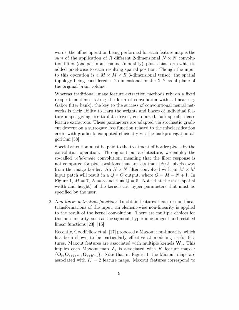
5 Experiments and ResultsThe experiments were carried out on real patient data obtained from the 2013brain tumor segmentation challenge (BRATS2013), as part of the MICCAIconference [14]. The BRATS2013 dataset is comprised of 3 sub-datasets. Thetraining dataset, which contains 30 patient subjects all with pixel-accurateground truth (20 high grade and 10 low grade tumors); the test dataset whichcontains 10 (all high grade tumors) and the leaderboard dataset which con-tains 25 patient subjects (21 high grade and 4 low grade tumors). There isno ground truth provided for the test and leaderboard datasets. All brains inthe dataset have the same orientation. For each brain there exists 4 modal-ities, namely T1, T1C, T2 and Flair which are co-registered. The trainingbrains come with groundtruth for which 5 segmentation labels are provided,namely non-tumor, necrosis, edema, non-enhancing tumor and enhancing tu-mor. Figure 4 shows an example of the data as well as the ground truth. Intotal, the model iterates over about 2.2 million examples of tumorous patches(this consists of all the 4 sub-tumor classes) and goes through 3.2 million ofthe healthy patches. As mentioned before during the first phase training,the distribution of examples introduced to the model from all 5 classes isuniform.
Please note that we could not use the BRATS 2014 dataset due to prob-lems with both the system performing the evaluation and the quality of the la-beled data. For these reasons the old BRATS 2014 dataset has been removedfrom the official website and, at the time of submitting this manuscript, theBRATS website still showed: “Final data for BRATS 2014 to be releasedsoon”. Furthermore, we have even conducted an experiment where we trainedour model with the old 2014 dataset and made predictions on the 2013 testdataset; however, the performance was worse than our results mentioned inthis paper. For these reasons, we decided to focus on the BRATS 2013 data.
As mentioned in Section 3, we work with 2D slices due to the fact thatthe MRI volumes in the dataset do not posses an isotropic resolution and
19

T1 T2 T1-enhanced Flair GT
Figure 4: The first four images from left to right show the MRI modalitiesused as input channels to various CNN models and the fifth image showsthe ground truth labels where � edema, � enhanced tumor, � necrosis, �non-enhanced tumor.
the spacing in the third dimension is not consistent across the data. Weexplored the use of 3D information (by treating the third dimension as extrainput channels or by having an architecture which takes orthogonal slicesfrom each view and makes the prediction on the intersecting center pixel),but that didn’t improve performance and made our method very slow.
Note that as suggested by Krizhevsky et al. [26], we applied data aug-mentation by flipping the input images. Unlike what was reported by Zeilerand Fergus [45], it did not improve the overall accuracy of our model.
Quantitative evaluation of the models performance on the test set isachieved by uploading the segmentation results to the online BRATS eval-uation system [13]. The online system provides the quantitative results asfollows: The tumor structures are grouped in 3 different tumor regions. Thisis mainly due to practical clinical applications. As described by Menze et al.[31], tumor regions are defined as:
1. The complete tumor region (including all four tumor structures).
2. The core tumor region (including all tumor structures exept “edema").
3. The enhancing tumor region (including the “enhanced tumor"structure).
For each tumor region, Dice (identical to F measure), Sensitivity andSpecificity are computed as follows :
Dice(P, T ) =|P1 ∧ T1|
(|P1|+ |T1|)/2,
20

Sensitivity(P, T ) =|P1 ∧ T1||T1|
,
Specificity(P, T ) =|P0 ∧ T0||T0|
,
where P represents the model predictions and T represents the groundtruth labels. We also note as T1 and T0 the subset of voxels predicted aspositives and negatives for the tumor region in question. Similarly for P1 andP0. The online evaluation system also provides a ranking for every methodsubmitted for evaluation. This includes methods from the 2013 BRATSchallenge published in [31] as well as anonymized unpublished methods forwhich no reference is available. In this section, we report experimental resultsfor our different CNN architectures.
5.1 The TwoPathCNN architecture
As mentioned previously, unlike conventional CNNs, the TwoPathCNN ar-chitecture has two pathways: a “local" path focusing on details and a “global"path more focused on the context. To better understand how joint trainingof the global and local pathways benefits the performance, we report resultson each pathway as well as results on averaging the outputs of each pathwaywhen trained separately. Our method also deals with the unbalanced natureof the problem by training in two phases as discussed in Section 3.2. Tosee the impact of the two phase training, we report results with and with-out it. We refer to the CNN model consisting of only the local path (i.e.conventional CNN architecture) as LocalPathCNN, the CNN model con-sisting of only the global path as GlobalPathCNN, the model averagingthe outputs of the local and global paths (i.e. LocalPathCNN and Glob-alPathCNN) as AverageCNN and the two-pathway CNN architecture asTwoPathCNN. The second training phase is noted by appending ‘*’ to thearchitecture name. Since the second phase training has a substantial effectand always improves the performance, we only report results on Global-PathCNN and AverageCNN with the second phase.
Table 1 presents the quantitative results of these variations. This tablecontains results for the TwoPathCNN with one and two training phases, thecommon single path CNN (i.e. LocalPathCNN) with one and two trainingphases, the GlobalPathCNN* which is a single path CNN model followingthe global pathway architecture and the output average of each of the trained
21

single-pathway models (AverageCNN*). Without much surprise, the singlepath with one training phase CNN was ranked last with the lowest scores onalmost every region. Using a second training phase gave a significant boostto that model with a rank that went from 15 to 9. Also, the table showsthat joint training of the local and global paths yields better performancecompared to when each pathway is trained separately and the outputs areaveraged. One likely explanation is that by joint training the local andglobal paths, the model allows the two pathways to co-adapt. In fact, theAverageCNN* performs worse than the LocalPathCNN* due to thefact that the GlobalPathCNN* performs very badly. The top performingmethod in the uncascaded models is the TwoPathCNN* with a rank of 4.
Also, in some cases results are less accurate over the Enhancing regionthan for the Core and Complete regions. There are 2 main reasons for that.First, borders are usually diffused and there are no clear cut between en-hanced tumor and non-enhanced tissues. This creates problems for bothuser labeling, ground truth, as well as the model. The second reason is thatthe model learns what it sees in the ground truth. Since the labels are cre-ated by different people and since the borders are not clear, each user has aslightly different interpretation of the borders of the enhanced tumor and sosometimes we see overly thick enhanced tumor in the ground truth.
Unfortunately, visualizing the learned mid/high level features of a CNNis still very much an open research problem. However, we can study theimpact these features have on predictions by visualizing the segmentationresults of different models. The segmentation results on two subjects fromour validation set, produced by different variations of the basic model canbe viewed in Figure 64. As shown in the figure, the two-phase trainingprocedure allows the model to learn from a more realistic distribution oflabels and thus removes false positives produced by the model which trainswith one training phase. Moreover, by having two pathways, the modelcan simultaneously learn the global contextual features as well as the localdetailed features. This gives the advantage of correcting labels at a globalscale as well as recognizing fine details of the tumor at a local scale, yieldinga better segmentation as oppose to a single path architecture which resultsin smoother boundaries. Joint training of the two convolutional pathwaysand having two training phases achieves better results.
4It is important to note that we do not train the model on the validation set and thusthe quality of the results is not due to overfitting
22

Second Phase
T1C Epoch = 5 Epoch = 11 Epoch = 25 Epoch = 35 Epoch = 55Epoch = 1
Epoch = 7Epoch = 5Epoch = 4Epoch = 2 Epoch = 10GT
Figure 5: Progression of learning in InputCascadeCNN*. The stream offigures on the first row from left to right show the learning process duringthe first phase. As the model learns better features, it can better distinguishboundaries between tumor sub-classes. This is made possible due to uniformlabel distribution of patches during the first phase training which makes themodel believe all classes are equiprobable and causes some false positives.This drawback is alleviated by training a second phase (shown in second rowfrom left to right) on a distribution closer to the true distribution of labels.The color codes are as follows: � edema, � enhanced tumor, � necrosis, �non-enhanced tumor.
Table 1: Performance of the TwoPathCNN model and variations. Thesecond phase training is noted by appending ‘*’ to the architecture name.The ‘Rank’ column represents the ranking of each method in the online scoreboard at the time of submission.
Rank Method Dice Specificity SensitivityComplete Core Enhancing Complete Core Enhancing Complete Core Enhancing
4 TwoPathCNN* 0.85 0.78 0.73 0.93 0.80 0.72 0.80 0.76 0.759 LocalPathCNN* 0.85 0.74 0.71 0.91 0.75 0.71 0.80 0.77 0.7310 AverageCNN* 0.84 0.75 0.70 0.95 0.83 0.73 0.77 0.74 0.7314 GlobalPathCNN* 0.82 0.73 0.68 0.93 0.81 0.70 0.75 0.65 0.7014 TwoPathCNN 0.78 0.63 0.68 0.67 0.50 0.59 0.96 0.89 0.8215 LocalPathCNN 0.77 0.64 0.68 0.65 0.52 0.60 0.96 0.87 0.80
23

LocalPathCNNT1C
GT LocalCascadeCNN*
LocalPathCNN LocalPathCNN*
TwoPathCNN*
T1C
LocalCascadeCNN* MFCascadeCNN* InputCascadeCNN*GT
GlobalPathCNN* AverageCNN*
GlobalPathCNN* AveragePathCNN*
MFCascadeCNN* InputCascadeCNN*
LocalPathCNN*
TwoPathCNN*
Figure 6: Visual results from our CNN architectures from the Axial view.For each sub-figure, the top row from left to right shows T1C modality, theconventional one path CNN, the Conventional CNN with two training phases,and the TwoPathCNN model. The second row from left to right shows theground truth, LocalCascadeCNN model, the MFCascadeCNN modeland the InputCascadeCNN. The color codes are as follows: � edema, �enhanced tumor, � necrosis, � non-enhanced tumor.
24
T1C GT InputCascadeCNN*
T1C GT InputCascadeCNN*
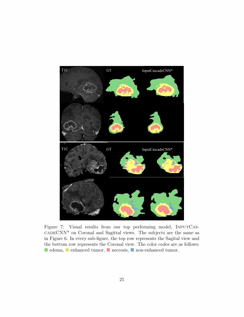
Figure 7: Visual results from our top performing model, InputCas-cadeCNN* on Coronal and Sagittal views. The subjects are the same asin Figure 6. In every sub-figure, the top row represents the Sagital view andthe bottom row represents the Coronal view. The color codes are as follows:� edema, � enhanced tumor, � necrosis, � non-enhanced tumor.
25
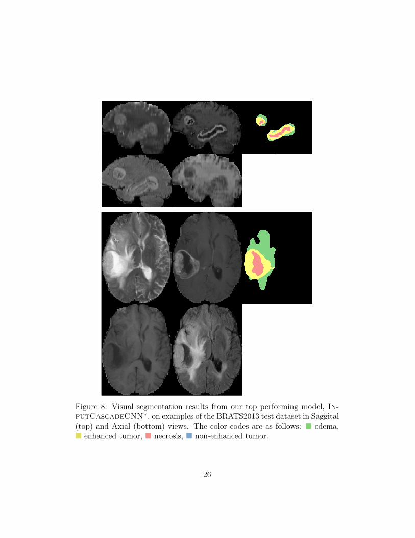
Figure 8: Visual segmentation results from our top performing model, In-putCascadeCNN*, on examples of the BRATS2013 test dataset in Saggital(top) and Axial (bottom) views. The color codes are as follows: � edema,� enhanced tumor, � necrosis, � non-enhanced tumor.
26

Table 2: Performance of the cascaded architectures. The reported resultsare from the second phase training. The ‘Rank’ column shows the rankingof each method in the online score board at the time of submission.
Rank Method Dice Specificity SensitivityComplete Core Enhancing Complete Core Enhancing Complete Core Enhancing
2 InputCascadeCNN* 0.88 0.79 0.73 0.89 0.79 0.68 0.87 0.79 0.804-a MFCascadeCNN* 0.86 0.77 0.73 0.92 0.80 0.71 0.81 0.76 0.764-c LocalCascadeCNN* 0.88 0.76 0.72 0.91 0.76 0.70 0.84 0.80 0.75
5.2 Cascaded architectures
We now discuss our experiments with the three cascaded architectures namelyInputCascadeCNN, LocalCascadeCNN and MFCascadeCNN. Ta-ble 2 provides the quantitative results for each architecture. Figure 6 alsoprovides visual examples of the segmentation generated by each architecture.
We find that the MFCascadeCNN* model yields smoother boundariesbetween classes. We hypothesize that, since the neurons in the softmaxoutput layer are directly connected to the previous outputs within each re-ceptive field, these parameters are more likely to learn that the center pixellabel should have a similar label to its surroundings.
As for the LocalCascadeCNN* architecture, while it resulted in fewerfalse positives in the complete tumor category, the performance in othercategories (i.e. tumor core and enhanced tumor) did not improve.
Figure 7 shows segmentation results from the same brains (as in Figure 6)in Sagittal and Coronal views. The InputCascadeCNN* model was usedto produce these results. As seen from this figure, although the segmentationis performed on Axial view but the output is consistent in Coronal and Sagit-tal views. Although subjects in Figure 5 and Figure 6 are from our validationset for which the model is not trained on and the segmentation results fromthese subjects can give a good estimate of the models performance on a testset, however, for further clarity we visualise the models performance on twosubjects from BRATS-2013 testst. These results are shown in Figure 8 inSaggital (top) and Axial (bottom) views.
To better understand the process for which InputCascadeCNN* learnsfeatures, we present in Figure 5 the progression of the model by makingpredictions at every few epochs on a subject from our validation set.
Overall, the best performance is reached by the InputCascadeCNN*
27

model. It improves the Dice measure on all tumor regions. With this architec-ture, we were able to reach the second rank on the BRATS 2013 scoreboard.While MFCascadeCNN*, TwoPathCNN* and LocalCascadeCNN*are all ranked 4, the inner ranking between these three models is noted as4a, 4b and 4c respectively.
Table 3 shows how our implemented architectures compare with currentlypublished state-of-the-art methods as mentioned in [31]5. The table showsthat InputCascadeCNN* out performs Tustison et al. the winner of theBRATS 2013 challenge and is ranked first in the table. Results from theBRATS-2013 leaderboard presented in Table 4 shows that our method out-performs other approaches on this dataset. We also compare our top per-forming method in Table 5 with state-of-the-art methods on BRATS-2012, 4label test set as mentioned in [31]. As seen from this table, our method outperforms other methods in the tumor Core category and gets competitiveresults on other categories.
Let us mention that Tustison’s method takes 100 minutes to computepredictions per brain as reported in [31], while the InputCascadeCNN*takes 3 minutes, thanks to the fully convolutional architecture and the GPUimplementation, which is over 30 times faster than the winner of the chal-lenge. The TwoPathCNN* has a performance close to the state-of-the-art.However, with a prediction time of 25 seconds, it is over 200 times fasterthan Tustison’s method. Other top methods in the table are that of Meier etal and Reza et al with processing times of 6 and 90 minutes respectively. Re-cently Subbanna et al. [41] published competitive results on the BRATS 2013dataset, reporting dice measures of 0.86, 0.86, 0.77 for Complete, Core andEnhancing tumor regions. Since they do not report Specificity and Sensitiv-ity measures, a completely fair comparison with that method is not possible.However, as mentioned in [41], their method takes 70 minutes to process asubject, which is about 23 times slower than our method.
Regarding other methods using CNNs, Urban et al. [43] used an averageof two 3D convolutional networks with dice measures of 0.87, 0.77, 0.73 forComplete, Core and Enhancing tumor regions on BRATS 2013 test datasetwith a prediction time of about 1 minute per model which makes for a totalof 2 minutes. Again, since they do not report Specificity and Sensitivity
5Please note that the results mentioned in Table 3 and Table 4 are from meth-ods competing in the BRATS 2013 challenge for which a static table is provided[https://www.virtualskeleton.ch/BRATS/StaticResults2013]. Since then, other methodshave been added to the score board but for which no reference is available.
28

Table 3: Comparison of our implemented architectures with the state-of-the-art methods on the BRATS-2013 test set.
Method Dice Specificity SensitivityComplete Core Enhancing Complete Core Enhancing Complete Core Enhancing
InputCascadeCNN* 0.88 0.79 0.73 0.89 0.79 0.68 0.87 0.79 0.80Tustison 0.87 0.78 0.74 0.85 0.74 0.69 0.89 0.88 0.83
MFCascadeCNN* 0.86 0.77 0.73 0.92 0.80 0.71 0.81 0.76 0.76TwoPathCNN* 0.85 0.78 0.73 0.93 0.80 0.72 0.80 0.76 0.75
LocalCascadeCNN* 0.88 0.76 0.72 0.91 0.76 0.70 0.84 0.80 0.75LocalPathCNN* 0.85 0.74 0.71 0.91 0.75 0.71 0.80 0.77 0.73
Meier 0.82 0.73 0.69 0.76 0.78 0.71 0.92 0.72 0.73Reza 0.83 0.72 0.72 0.82 0.81 0.70 0.86 0.69 0.76Zhao 0.84 0.70 0.65 0.80 0.67 0.65 0.89 0.79 0.70
Cordier 0.84 0.68 0.65 0.88 0.63 0.68 0.81 0.82 0.66TwoPathCNN 0.78 0.63 0.68 0.67 0.50 0.59 0.96 0.89 0.82
LocalPathCNN 0.77 0.64 0.68 0.65 0.52 0.60 0.96 0.87 0.80Festa 0.72 0.66 0.67 0.77 0.77 0.70 0.72 0.60 0.70Doyle 0.71 0.46 0.52 0.66 0.38 0.58 0.87 0.70 0.55
Table 4: Comparison of our top implemented architectures with the state-of-the-art methods on the BRATS-2013 leaderboard set.
Method Dice Specificity SensitivityComplete Core Enhancing Complete Core Enhancing Complete Core Enhancing
InputCascadeCNN* 0.84 0.71 0.57 0.88 0.79 0.54 0.84 0.72 0.68Tustison 0.79 0.65 0.53 0.83 0.70 0.51 0.81 0.73 0.66Zhao 0.79 0.59 0.47 0.77 0.55 0.50 0.85 0.77 0.53Meier 0.72 0.60 0.53 0.65 0.62 0.48 0.88 0.69 0.6Reza 0.73 0.56 0.51 0.68 0.64 0.48 0.79 0.57 0.63
Cordier 0.75 0.61 0.46 0.79 0.61 0.43 0.78 0.72 0.52
measures, we can not make a full comparison. However, based on their dicescores our TwoPathCNN* is similar in performance while taking only 25seconds, which is four times faster. And the InputCascadeCNN* is betteror equal in accuracy while having the same processing time. As for [46], theydo not report results on BRATS 2013 test dataset. However, their method isvery similar to the LocalPathCNN which, according to our experiments,has worse performance.
29

Table 5: Comparison of our top implemented architectures with the state-of-the-art methods on the BRATS-2012 4 label test set.
Method DiceComplete Core Enhancing
InputCascadeCNN* 0.81 0.72 0.58Subbanna 0.75 0.70 0.59
Zhao 0.82 0.66 0.42Tustison 0.75 0.55 0.52Festa 0.62 0.50 0.61
6 ConclusionIn this paper, we presented an automatic brain tumor segmentation methodbased on deep convolutional neural networks. We considered different archi-tectures and investigated their impact on the performance. Results from theBRATS 2013 online evaluation system confirms that with our best model wemanaged to improve on the currently published state-of-the-art method bothon accuracy and speed as presented in MICCAI 2013. The high performanceis achieved with the help of a novel two-pathway architecture (which canmodel both the local details and global context) as well as modeling locallabel dependencies by stacking two CNN’s. Training is based on a two phaseprocedure, which we’ve found allows us to train CNNs efficiently when thedistribution of labels is unbalanced.
Thanks to the convolutional nature of the models and by using an effi-cient GPU implementation, the resulting segmentation system is very fast.The time needed to segment an entire brain with any of the these CNN ar-chitectures varies between 25 seconds and 3 minutes, making them practicalsegmentation methods.
References[1] Alvarez, J.M., Gevers, T., LeCun, Y., Lopez, A.M., 2012. Road scene segmen-
tation from a single image, in: Proceedings of the 12th European Conferenceon Computer Vision - Volume Part VII, Springer-Verlag, Berlin, Heidelberg.pp. 376–389.
[2] Angelini, E., Clatz, O., E., Konukoglu, E., Capelle, L., Duffau, H., 2007.
30

Glioma dynamics and computational models: A review of segmentation, reg-istration, and in silico growth algorithms and their clinical applications 3.
[3] Avants, B.B., Tustison, N., Song, G., 2009. Advanced normalization tools(ants). Insight J .
[4] Bauer, S., Nolte, L.P., Reyes, M., 2011. Fully automatic segmentation of braintumor images using support vector machine classification in combination withhierarchical conditional random field regularization., in: MICCAI, pp. 354–361.
[5] Bauer, S., Wiest, R., Nolte, L., Reyes, M., 2013. A survey of mri-based medicalimage analysis for brain tumor studies. Physics in medicine and biology 58,97–129.
[6] Bengio, Y., 2012. Practical recommendations for gradient-based training ofdeep architectures, in: Neural Networks: Tricks of the Trade. Springer, pp.437–478.
[7] Bengio, Y., Courville, A., Vincent, P., 2013. Representation learning: Areview and new perspectives. Pattern Analysis and Machine Intelligence, IEEETransactions on 35, 1798–1828.
[8] Clark, M., Hall, L., Goldgof, D., Velthuizen, R.P., Murtagh, F., Silbiger, M.L.,1998. Automatic tumor segmentation using knowledge-based clustering. IEEETrans. Med. Imaging 17, 187–201.
[9] Cobzas, D., Birkbeck, N., Schmidt, M., Jägersand, M., Murtha, A., 2007. 3dvariational brain tumor segmentation using a high dimensional feature set, in:ICCV, pp. 1–8.
[10] Davy, A., Havaei, M., Warde-Farley, D., Biard, A., Tran, L., Jodoin, P.M.,Courville, A., Larochelle, H., Pal, C., Bengio, Y., 2014. Brain tumor segmen-tation with deep neural networks. in proc of BRATS-MICCAI .
[11] Doyle, S., Vasseur, F., Dojat, M., Forbes, F., 2013. Fully automatic braintumor segmentation from multiple mr sequences using hidden markov fieldsand variational em. in proc of BRATS-MICCAI .
[12] Farabet, C., Couprie, C., Najman, L., LeCun, Y., 2013. Learning hierarchicalfeatures for scene labeling. Pattern Analysis and Machine Intelligence, IEEETransactions on 35, 1915–1929.
31

[13] Farahani, K., Menze, B., Reyes, M., 2013. Multimodal Brain Tumor Segmen-tation (BRATS 2013). URL: http://martinos.org/qtim/miccai2013/.
[14] Farahani, K., Menze, B., Reyes, M., 2014. Brats 2014 Challenge Manuscripts.URL: http://www.braintumorsegmentation.org.
[15] Glorot, X., Bordes, A., Bengio, Y., 2011. Domain adaptation for large-scalesentiment classification: A deep learning approach, in: Proceedings of the28th International Conference on Machine Learning (ICML-11), pp. 513–520.
[16] Goodfellow, I.J., Warde-Farley, D., Lamblin, P., Dumoulin, V., Mirza, M.,Pascanu, R., Bergstra, J., Bastien, F., Bengio, Y., 2013a. Pylearn2: a machinelearning research library. arXiv preprint arXiv:1308.4214 .
[17] Goodfellow, I.J., Warde-Farley, D., Mirza, M., Courville, A., Bengio, Y.,2013b. Maxout networks, in: ICML.
[18] Gotz, M., Weber, C., Blocher, J., Stieltjes, B., Meinzer, H.P., Maier-Hein, K.,2014. Extremely randomized trees based brain tumor segmentation, in: inproc of BRATS Challenge - MICCAI.
[19] Hamamci, A., Kucuk, N., Karaman, K., Engin, K., Unal, G., 2012. Tumor-cut:Segmentation of brain tumors on contrast enhanced mr images for radiosurgeryapplications. IEEE trans. Medical Imaging 31, 790–804.
[20] Hariharan, B., Arbeláez, P., Girshick, R., Malik, J., 2014. Simultaneous de-tection and segmentation, in: Computer Vision–ECCV 2014. Springer, pp.297–312.
[21] Havaei, M., Jodoin, P.M., Larochelle, H., 2014. Efficient interactive braintumor segmentation as within-brain knn classification, in: International Con-ference on Pattern Recognition (ICPR).
[22] Huang, G.B., Jain, V., 2013. Deep and wide multiscale recursive networks forrobust image labeling. arXiv preprint arXiv:1310.0354 .
[23] Jarrett, K., Kavukcuoglu, K., Ranzato, M., LeCun, Y., 2009. What is thebest multi-stage architecture for object recognition?, in: Computer Vision,2009 IEEE 12th International Conference on, IEEE. pp. 2146–2153.
[24] Khotanlou, H., Colliot, O., Atif, J., Bloch, I., 2009. 3d brain tumor seg-mentation in mri using fuzzy classification, symmetry analysis and spatiallyconstrained deformable models. Fuzzy Sets Syst. 160, 1457–1473.
32

[25] Kleesiek, J., Biller, A., Urban, G., Kothe, U., Bendszus, M., Hamprecht, F.A.,2014. ilastik for multi-modal brain tumor segmentation. in proc of BRATS-MICCAI .
[26] Krizhevsky, A., Sutskever, I., Hinton, G., 2012. ImageNet classification withdeep convolutional neural networks, in: NIPS.
[27] Kwon, D., Akbari, H., Da, X., Gaonkar, B., Davatzikos, C., 2014. Multimodalbrain tumor image segmentation using glistr, in: in proc of BRATS Challenge- MICCAI.
[28] LeCun, Y., Bottou, L., Bengio, Y., Haffner, P., 1998. Gradient-based learningapplied to document recognition. Proceedings of the IEEE 86, 2278–2324.
[29] Lee, C.H., Schmidt, M., Murtha, A., Bistritz, A., S, J., Greiner, R., 2005.Segmenting brain tumor with conditional random fields and support vectormachines, in: in Proc of Workshop on Computer Vision for Biomedical ImageApplications.
[30] Long, J., Shelhamer, E., Darrell, T., 2015. Fully convolutional networks forsemantic segmentation. CVPR (to appear) .
[31] Menze, B., Reyes, M., Leemput, K.V., 2014. The multimodal brain tumorimage segmentation benchmark (brats). IEEE Trans. on Medical Imaging(accepted) .
[32] N.Tustison, M. Wintermark, C.D., Avants, B., 2013. Ants and árboles, in: inproc of BRATS Challenge - MICCAI.
[33] Parisot, S., Duffau, H., Chemouny, S., Paragios, N., 2012. Joint tumor segmen-tation and dense deformable registration of brain mr images., in: MICCAI,pp. 651–658.
[34] Pinheiro, P., Collobert, R., 2014. Recurrent convolutional neural networksfor scene labeling, in: Proceedings of The 31st International Conference onMachine Learning, pp. 82–90.
[35] Popuri, K., Cobzas, D., Murtha, A., Jägersand, M., 2012. 3d variational braintumor segmentation using dirichlet priors on a clustered feature set. Int. J.Computer Assisted Radiology and Surgery 7, 493–506.
[36] Prastawa, M., Bullit, E., Ho, S., Gerig, G., 2004. A brain tumor segmentationframework based on outlier detection. Medical Image Anaylsis 8, 275–283.
33

[37] Prastawa, M., Bullitt, E., Ho, S., Gerig, G., 2003. Robust estimation for braintumor segmentation, in: Medical Image Computing and Computer-AssistedIntervention-MICCAI 2003. Springer, pp. 530–537.
[38] Rumelhart, D.E., Hinton, G.E., Williams, R.J., 1988. Learning representationsby back-propagating errors. Cognitive modeling 5.
[39] Schmidt, M., Levner, I., Greiner, R., Murtha, A., Bistritz, A., 2005. Segment-ing brain tumors using alignment-based features, in: Int. Conf on MachineLearning and Applications, pp. 6–pp.
[40] Srivastava, N., Hinton, G., Krizhevsky, A., Sutskever, I., Salakhutdinov, R.,2014. Dropout: A simple way to prevent neural networks from overfitting.Journal of Machine Learning Research 15, 1929–1958. URL: http://jmlr.org/papers/v15/srivastava14a.html.
[41] Subbanna, N., Precup, D., Arbel, T., 2014. Iterative multilevel mrf leveragingcontext and voxel information for brain tumour segmentation in mri.
[42] Subbanna, N., Precup, D., Collins, L., Arbel, T., 2013. Hierarchical proba-bilistic gabor and mrf segmentation of brain tumours in mri volumes., in: inproc of MICCAI, pp. 751–758.
[43] Urban, G., Bendszus, M., Hamprecht, F., Kleesiek, J., 2014. Multi-modalbrain tumor segmentation using deep convolutional neural networks. in procof BRATS-MICCAI .
[44] Xing, E.P., Jordan, M.I., Russell, S., 2002. A generalized mean field algorithmfor variational inference in exponential families, in: Proceedings of the Nine-teenth conference on Uncertainty in Artificial Intelligence, Morgan KaufmannPublishers Inc.. pp. 583–591.
[45] Zeiler, M.D., Fergus, R., 2014. Visualizing and understanding convolutionalnetworks, in: Computer Vision–ECCV 2014. Springer, pp. 818–833.
[46] Zikic, D., Ioannou, Y., Brown, M., Criminisi, A., 2014. Segmentation of braintumor tissues with convolutional neural networks. in proc of BRATS-MICCAI.
34