Boundary Value Problems for Partial Differential …nguyen.hong.hai.free.fr/EBOOKS/SCIENCE AND ENGINEERING...Chapter 9 Boundary Value Problems for Partial Differential Equations 9.1

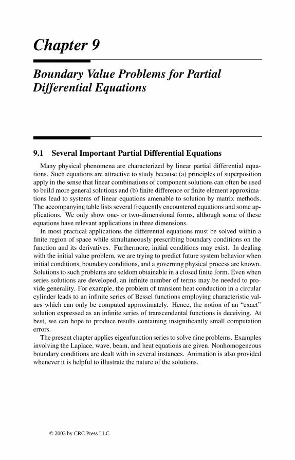
Chapter 9

Boundary Value Problems for PartialDifferential Equations

9.1 Several Important Partial Differential Equations

Many physical phenomena are characterized by linear partial differential equa-tions. Such equations are attractive to study because (a) principles of superpositionapply in the sense that linear combinations of component solutions can often be usedto build more general solutions and (b) Þnite difference or Þnite element approxima-tions lead to systems of linear equations amenable to solution by matrix methods.The accompanying table lists several frequently encountered equations and some ap-plications. We only show one- or two-dimensional forms, although some of theseequations have relevant applications in three dimensions.

In most practical applications the differential equations must be solved within aÞnite region of space while simultaneously prescribing boundary conditions on thefunction and its derivatives. Furthermore, initial conditions may exist. In dealingwith the initial value problem, we are trying to predict future system behavior wheninitial conditions, boundary conditions, and a governing physical process are known.Solutions to such problems are seldom obtainable in a closed Þnite form. Even whenseries solutions are developed, an inÞnite number of terms may be needed to pro-vide generality. For example, the problem of transient heat conduction in a circularcylinder leads to an inÞnite series of Bessel functions employing characteristic val-ues which can only be computed approximately. Hence, the notion of an exactsolution expressed as an inÞnite series of transcendental functions is deceiving. Atbest, we can hope to produce results containing insigniÞcantly small computationerrors.

The present chapter applies eigenfunction series to solve nine problems. Examplesinvolving the Laplace, wave, beam, and heat equations are given. Nonhomogeneousboundary conditions are dealt with in several instances. Animation is also providedwhenever it is helpful to illustrate the nature of the solutions.

© 2003 by CRC Press LLC

Equation Equation ApplicationsName

uxx + uyy = αut Heat Transient heat conduction

uxx + uyy = αutt Wave Transverse vibrations of membranesand other wave type phenomena

uxx + uyy = 0 Laplace Steady-state heat conduction andelectrostatics

uxx + uyy = f(x, y) Poisson Stress analysis of linearly elasticbodies

uxx + uyy + ω2u = 0 Helmholtz Steady-state harmonic vibrationproblems

EIyxxxx = −Aρytt + f(x, t) Beam Transverse ßexural vibrations ofelastic beams

9.2 Solving the Laplace Equation inside a Rectangular Region

Functions which satisfy Laplaces equation are encountered often in practice. Suchfunctions are called harmonic; and the problem of determining a harmonic functionsubject to given boundary values is known as the Dirichlet problem [119]. In afew cases with simple geometries, the Dirichlet problem can be solved explicitly.One instance is a rectangular region with the boundary values of the function beingexpandable in a Fourier sine series. The following program employs the FFT to con-struct a solution for boundary values represented by piecewise linear interpolation.Surface and contour plots of the resulting Þeld values are also presented.

The problem of interest satisÞes the differential equation

∂2u

∂x2+∂2u

∂y2= 0 , 0 < x < a , 0 < y < b

with the boundary conditions of the form

u(x, 0) = F (x) , 0 < x < a ,

u(x, b) = G(x) , 0 < x < a ,

u(0, y) = P (y) , 0 < y < b ,

u(a, y) = Q(y) , 0 < y < b .

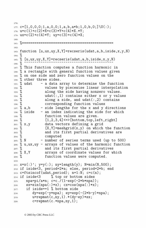
The series solution can be represented as

u(x, y) =∞∑

n=1

fnan(x, y) + gnan(x, b− y) + pnbn(x, y) + qnbn(a− x, y)


where

an(x, y) = sin[nπxa

]sinh

[nπ(b− y)

a

]/ sinh

[nπb

a

],

bn(x, y) = sinh[nπ(a− x)

b

]sin

[nπyb

]/ sinh

[nπab

],

and the constants fm, gm, pn, and qn are coefÞcients in the Fourier sine expansionsof the boundary value functions. This implies that

F (x) =∞∑

n=1

fn sin[nπxa

], G(x) =

∞∑n=1

gn sin[nπxa

],

P (y) =∞∑

n=1

pn sin[nπyb

], Q(y) =

∞∑n=1

qn sin[nπyb

].

The coefÞcients in the series can be computed by integration as

fn =2a

∫ a

0

F (x) sin[nπxa

]dx , gn =

2a

∫ a

0

G(x) sin[nπxa

]dx,

pn =2a

∫ b

0

P (y) sin[nπyb

]dy , qn =

2a

∫ b

0

Q(y) sin[nπyb

]dy,

or approximate coefÞcients can be obtained using the FFT. The latter approach ischosen here and the solution is evaluated for an arbitrary number of terms in theseries.

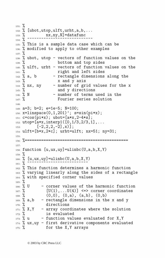
The chosen problem solution has the disadvantage of employing eigenfunctionsthat vanish at the ends of the expansion intervals. Consequently, it is desirable tocombine the series with an additional term allowing exact satisfaction of the cornerconditions for cases where the boundary value functions for adjacent sides agree.This implies requirements such as F (a) = Q(0) and three other similar conditions.It is evident that the function

up(x, y) = c1 + c2x+ c3y + c4xy

is harmonic and varies linearly along each side of the rectangle. Constants c 1, · · · , c4can be computed to satisfy the corner values and the total solution is represented asup plus a series solution involving modiÞed boundary conditions.

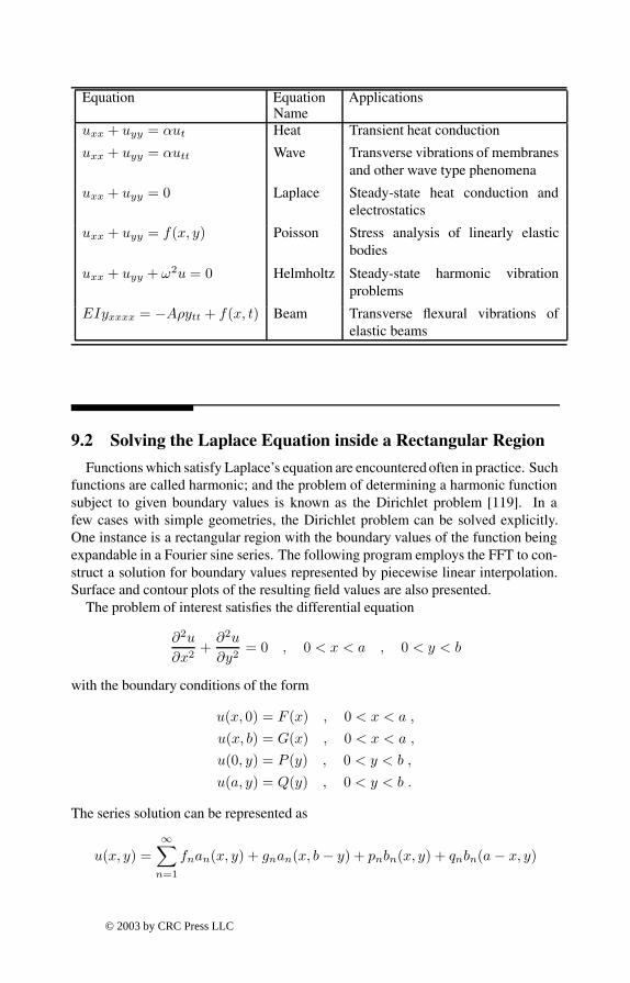
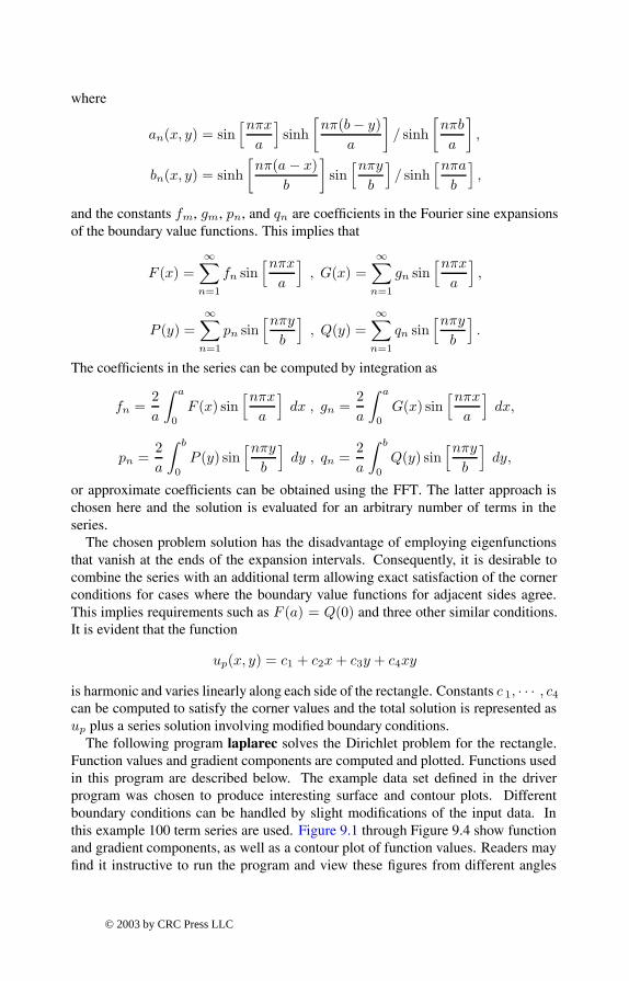
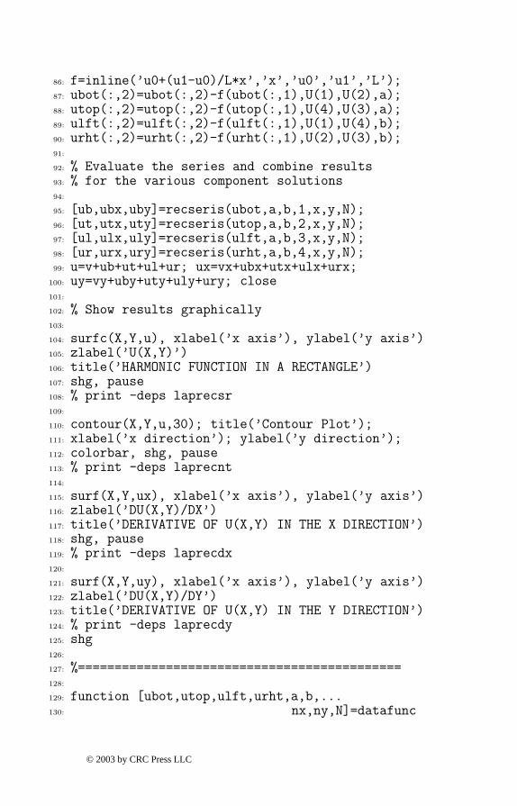
The following program laplarec solves the Dirichlet problem for the rectangle.Function values and gradient components are computed and plotted. Functions usedin this program are described below. The example data set deÞned in the driverprogram was chosen to produce interesting surface and contour plots. Differentboundary conditions can be handled by slight modiÞcations of the input data. Inthis example 100 term series are used. Figure 9.1 through Figure 9.4 show functionand gradient components, as well as a contour plot of function values. Readers mayÞnd it instructive to run the program and view these Þgures from different angles


laplarec inputs data, calls computation modules, andplots results

datafunc deÞnes an example datacaseulinbc particular solution for linearly varying

boundary conditionsrecseris sums the series for function and gradient val-

uessincof generates coefÞcients in a Fourier sine serieslintrp piecewise linear interpolation function allow-

ing jump discontinuities

using the interactive Þgure rotating capability provided in MATLAB. Note that theÞgure showing the function gradient in the x direction used view([225,20]) to showclearly the jump discontinuity in this quantity.


00.5

11.5

22.5

3

0

0.5

1

1.5

2−2

−1.5

−1

−0.5

0

0.5

1

1.5

2

2.5

x axis

HARMONIC FUNCTION IN A RECTANGLE

y axis

U(X

,Y)

Figure 9.1: Surface Plot of Function Values

0 0.5 1 1.5 2 2.5 30

0.2

0.4

0.6

0.8

1

1.2

1.4

1.6

1.8

2Contour Plot

x direction

y di

rect

ion

−1.5

−1

−0.5

0

0.5

1

1.5

Figure 9.2: Contour Plot of Function Values


00.5

11.5

22.5

3 0

0.5

1

1.5

2

−5

−4

−3

−2

−1

0

1

2

3

4

5

y axis

DERIVATIVE OF U(X,Y) IN THE X DIRECTION

x axis

DU

(X,Y

)/D

X

Figure 9.3: Function Derivative in the x Direction

00.5

11.5

22.5

3

0

0.5

1

1.5

2−4

−2

0

2

4

6

8

x axis

DERIVATIVE OF U(X,Y) IN THE Y DIRECTION

y axis

DU

(X,Y

)/D

Y

Figure 9.4: Function Derivative in the y Direction


MATLAB Example

Program laplarec

1: function [u,ux,uy,X,Y]=laplarec(...2: ubot,utop,ulft,urht,a,b,nx,ny,N)3: %4: % [u,ux,uy,X,Y]=laplarec(...5: % ubot,utop,ulft,urht,a,b,nx,ny,N)6: % ~~~~~~~~~~~~~~~~~~~~~~~~~~~~~~~~~~~~~~~~~~~~~7: % This program evaluates a harmonic function and its8: % first partial derivatives in a rectangular region.9: % The method employs a Fourier series expansion.

10: % ubot - defines the boundary values on the bottom11: % side. This can be an array in which12: % ubot(:,1) is x coordinates and ubot(:,2)13: % is function values. Values at intermediate14: % points are obtained by piecewise linear15: % interpolation. A character string giving16: % the name of a function can also be used.17: % Then the function is evualuated using 20018: % points along a side to convert ubot to an19: % array. Similar comments apply for utop,20: % ulft, and urht introduced below.21: % utop - boundary value definition on the top side22: % ulft - boundary value definition on the left side23: % urht - boundary value definition on the right side24: % a,b - rectangle dimensions in x and y directions25: % nx,ny - number of x and y values for which the26: % solution is evaluated27: % N - number of terms used in the Fourier series28: % u - function value for the solution29: % ux,uy - first partial derivatives of the solution30: % X,Y - coordinate point arrays where the solution31: % is evaluated32: %33: % User m functions used: datafunc ulinbc34: % recseris ftsincof35:

36: disp(’ ’)37: disp(’SOLVING THE LAPLACE EQUATION IN A RECTANGLE’)38: disp(’ ’)39:

40: if nargin==0


41: disp(...42: ’Give the name of a function defining the data’)43: datfun=input(...44: ’(try datafunc as an example): > ? ’,’s’);45: [ubot,utop,ulft,urht,a,b,nx,ny,N]=feval(datfun);46: end47:

48: % Create a grid to evaluate the solution49: x=linspace(0,a,nx); y=linspace(0,b,ny);50: [X,Y]=meshgrid(x,y); d=(a+b)/1e6;51: xd=linspace(0,a,201)’; yd=linspace(0,b,201)’;52:

53: % Check whether boundary values are given using54: % external functions. Convert these to arrays55:

56: if isstr(ubot)57: ud=feval(ubot,xd); ubot=[xd,ud(:)];58: end59: if isstr(utop)60: ud=feval(utop,xd); utop=[xd,ud(:)];61: end62: if isstr(ulft)63: ud=feval(ulft,yd); ulft=[yd,ud(:)];64: end65: if isstr(urht)66: ud=feval(urht,yd); urht=[yd,ud(:)];67: end68:

69: % Determine function values at the corners70: ub=interp1(ubot(:,1),ubot(:,2),[d,a-d]);71: ut=interp1(utop(:,1),utop(:,2),[d,a-d]);72: ul=interp1(ulft(:,1),ulft(:,2),[d,b-d]);73: ur=interp1(urht(:,1),urht(:,2),[d,b-d]);74: U=[ul(1)+ub(1),ub(2)+ur(1),ur(2)+ut(2),...75: ut(1)+ul(2)]/2;76:

77: % Obtain a solution satisfying the corner78: % values and varying linearly along the sides79:

80: [v,vx,vy]=ulinbc(U,a,b,X,Y);81:

82: % Reduce the corner values to zero to improve83: % behavior of the Fourier series solution84: % near the corners85:


86: f=inline(’u0+(u1-u0)/L*x’,’x’,’u0’,’u1’,’L’);87: ubot(:,2)=ubot(:,2)-f(ubot(:,1),U(1),U(2),a);88: utop(:,2)=utop(:,2)-f(utop(:,1),U(4),U(3),a);89: ulft(:,2)=ulft(:,2)-f(ulft(:,1),U(1),U(4),b);90: urht(:,2)=urht(:,2)-f(urht(:,1),U(2),U(3),b);91:

92: % Evaluate the series and combine results93: % for the various component solutions94:

95: [ub,ubx,uby]=recseris(ubot,a,b,1,x,y,N);96: [ut,utx,uty]=recseris(utop,a,b,2,x,y,N);97: [ul,ulx,uly]=recseris(ulft,a,b,3,x,y,N);98: [ur,urx,ury]=recseris(urht,a,b,4,x,y,N);99: u=v+ub+ut+ul+ur; ux=vx+ubx+utx+ulx+urx;

100: uy=vy+uby+uty+uly+ury; close101:

102: % Show results graphically103:

104: surfc(X,Y,u), xlabel(’x axis’), ylabel(’y axis’)105: zlabel(’U(X,Y)’)106: title(’HARMONIC FUNCTION IN A RECTANGLE’)107: shg, pause108: % print -deps laprecsr109:

110: contour(X,Y,u,30); title(’Contour Plot’);111: xlabel(’x direction’); ylabel(’y direction’);112: colorbar, shg, pause113: % print -deps laprecnt114:

115: surf(X,Y,ux), xlabel(’x axis’), ylabel(’y axis’)116: zlabel(’DU(X,Y)/DX’)117: title(’DERIVATIVE OF U(X,Y) IN THE X DIRECTION’)118: shg, pause119: % print -deps laprecdx120:

121: surf(X,Y,uy), xlabel(’x axis’), ylabel(’y axis’)122: zlabel(’DU(X,Y)/DY’)123: title(’DERIVATIVE OF U(X,Y) IN THE Y DIRECTION’)124: % print -deps laprecdy125: shg126:

127: %============================================128:

129: function [ubot,utop,ulft,urht,a,b,...130: nx,ny,N]=datafunc


131: %132: % [ubot,utop,ulft,urht,a,b,...133: % nx,ny,N]=datafunc134: % ~~~~~~~~~~~~~~~~~~~~~~~~~~~~135: % This is a sample data case which can be136: % modified to apply to other examples137: %138: % ubot, utop - vectors of function values on the139: % bottom and top sides140: % ulft, urht - vectors of function values on the141: % right and left sides142: % a, b - rectangle dimensions along the143: % x and y axis144: % nx, ny - number of grid values for the x145: % and y directions146: % N - number of terms used in the147: % Fourier series solution148:

149: a=3; b=2; e=1e-5; N=100;150: x=linspace(0,1,201)’; s=sin(pi*x);151: c=cos(pi*x); ubot=[a*x,2-4*s];152: utop=[a*x,interp1([0,1/3,2/3,1],...153: [-2,2,2,-2],x)];154: ulft=[b*x,2*c]; urht=ulft; nx=51; ny=31;155:

156: %============================================157:

158: function [u,ux,uy]=ulinbc(U,a,b,X,Y)159: %160: % [u,ux,uy]=ulinbc(U,a,b,X,Y)161: % ~~~~~~~~~~~~~~~~~~~~~~~~~~162: % This function determines a harmonic function163: % varying linearly along the sides of a rectangle164: % with specified corner values165: %166: % U - corner values of the harmonic function167: % [U(1),...U(4)] <=> corner coordinates168: % (0,0), (0,a), (a,b), (0,b)169: % a,b - rectangle dimensions in the x and y170: % directions171: % X,Y - array coordinates where the solution172: % is evaluated173: % u - function values evaluated for X,Y174: % ux,uy - first derivative components evaluated175: % for the X,Y arrays


176:

177: c=[1,0,0,0;1,a,0,0;1,a,b,a*b;1,0,b,0;]\U(:);178: u=c(1)+c(2)*X+c(3)*Y+c(4)*X.*Y;179: ux=c(2)+c(4)*Y; uy=c(3)+c(4)*X;180:

181: %============================================182:

183: function [u,ux,uy,X,Y]=recseris(udat,a,b,iside,x,y,N)184: %185: % [u,ux,uy,X,Y]=recseris(udat,a,b,iside,x,y,N)186: % ~~~~~~~~~~~~~~~~~~~~~~~~~~~~~~~~~~~~~~~~~~~187: % This function computes a function harmonic in188: % a rectangle with general function values given189: % on one side and zero function values on the190: % other three sides.191: % udat - a data array to determine the function192: % values by piecewise linear interpolation193: % along the side having nonzero values.194: % udat(:,1) contains either x or y values195: % along a side, and udat(:,2) contains196: % corresponding function values197: % a,b - side lengths for the x and y directions198: % iside - an index indicating the side for which199: % function values are given.200: % [1,2,3,4]<=>[bottom,top,left,right]201: % x,y data vectors defining a grid202: % [X,Y]=meshgrid(x,y) on which the function203: % and its first partial derivatives are204: % computed205: % N - number of series terms used (up to 500)206: % u,ux,uy - arrays of values of the harmonic function207: % and its first partial derivatives208: % X,Y arrays of coordinate values for which209: % function values were computed.210:

211: x=x(:)’; y=y(:); ny=length(y); N=min(N,500);212: if iside<3, period=2*a; else, period=2*b; end213: c=ftsincof(udat,period); n=1:N; c=c(n);214: if iside<3 % top or bottom sides215: npa=pi/a*n; c=c./(1-exp(-2*b*npa));216: sx=sin(npa(:)*x); cx=cos(npa(:)*x);217: if iside==1 % bottom side218: dy=exp(-y*npa); ey=exp(-(2*b-y)*npa);219: u=repmat(c,ny,1).*(dy-ey)*sx;220: c=repmat(c.*npa,ny,1);


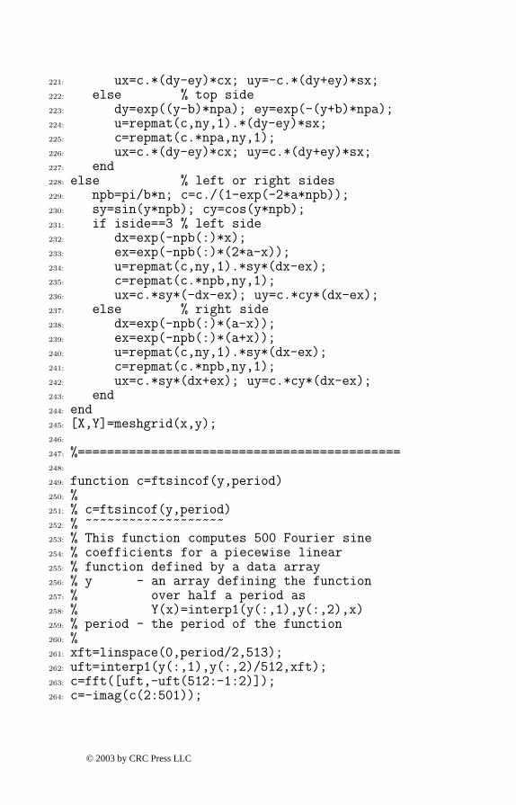
221: ux=c.*(dy-ey)*cx; uy=-c.*(dy+ey)*sx;222: else % top side223: dy=exp((y-b)*npa); ey=exp(-(y+b)*npa);224: u=repmat(c,ny,1).*(dy-ey)*sx;225: c=repmat(c.*npa,ny,1);226: ux=c.*(dy-ey)*cx; uy=c.*(dy+ey)*sx;227: end228: else % left or right sides229: npb=pi/b*n; c=c./(1-exp(-2*a*npb));230: sy=sin(y*npb); cy=cos(y*npb);231: if iside==3 % left side232: dx=exp(-npb(:)*x);233: ex=exp(-npb(:)*(2*a-x));234: u=repmat(c,ny,1).*sy*(dx-ex);235: c=repmat(c.*npb,ny,1);236: ux=c.*sy*(-dx-ex); uy=c.*cy*(dx-ex);237: else % right side238: dx=exp(-npb(:)*(a-x));239: ex=exp(-npb(:)*(a+x));240: u=repmat(c,ny,1).*sy*(dx-ex);241: c=repmat(c.*npb,ny,1);242: ux=c.*sy*(dx+ex); uy=c.*cy*(dx-ex);243: end244: end245: [X,Y]=meshgrid(x,y);246:

247: %============================================248:

249: function c=ftsincof(y,period)250: %251: % c=ftsincof(y,period)252: % ~~~~~~~~~~~~~~~~~~~253: % This function computes 500 Fourier sine254: % coefficients for a piecewise linear255: % function defined by a data array256: % y - an array defining the function257: % over half a period as258: % Y(x)=interp1(y(:,1),y(:,2),x)259: % period - the period of the function260: %261: xft=linspace(0,period/2,513);262: uft=interp1(y(:,1),y(:,2)/512,xft);263: c=fft([uft,-uft(512:-1:2)]);264: c=-imag(c(2:501));


9.3 The Vibrating String

Transverse motion of a tightly stretched string illustrates one of the simplest oc-currences of one-dimensional wave propagation. The transverse deßection satisÞesthe wave equation

a2 ∂2u

∂X2=∂2u

∂T 2

where u(X,T ) satisÞes initial conditions

u(X, 0) = F (X) ,∂u(X, 0)∂T

= G(X)

with boundary conditions

u(0, T ) = 0 , u(, T ) = 0

where is the string length. If we introduce the dimensionless variables x = X/and t = T/(/a) the differential equation becomes

uxx = utt

where subscripts denote partial differentiation. The boundary conditions become

u(0, t) = u(1, t) = 0

and the initial conditions become

u(x, 0) = f(x) , ut(x, 0) = g(x).

Let us consider the case where the string is released from rest initially so g(x) = 0.The solution can be found in series form as

u(x, t) =∞∑

n=1

anpn(x) cos(ωnt)

where ωn are natural frequencies and satisfaction of the differential equation of mo-tion requires

p′′n(x) + ω2npn(x) = 0

sopn = An sin(ωnx) +Bn cos(ωnx).

The boundary condition pn(0) = Bn = 0 and pn(1) = An sin(ωn) requiresAn = 0and ωn = nπ, where n is an integer. This leads to a solution in the form

u(x, t) =∞∑

n=1

an sin(nπx) cos(nπt).


The remaining condition on initial conditions requires

∞∑n=1

an sin(nπx) = f(x) , 0 < x < 1.

Therefore, the coefÞcients an are obtainable from an odd-valued Fourier series ex-pansion of f(x) vanishing at x = 0 and x = 2. We see that f(−x) = −f(x) andf(x+ 2) = f(x), and the coefÞcients are obtainable by integration as

an = 2∫ 1

0

f(x) sin(nπx) dx.

However, an easier way to compute the coefÞcients is to use the FFT. A solution willbe given for an arbitrary piecewise linear initial condition.

Before implementing the Fourier series solution, let us digress brießy to examinethe case of an inÞnite string governed by

a2uXX = uTT , −∞ < X <∞

and initial conditions

u(X, 0) = F (X) , uT (X, 0) = G(X).

The reader can verify directly that the solution of this problem is given by

u(X,T ) =12

[F (X − aT ) + F (X + aT )] +12a

∫ X+aT

X−aT

G(x) dx.

When the string is released from rest, G(X) is zero and the solution reduces to

F (X − aT ) + F (X + aT )2

which shows that the initial deßection splits into two parts with one half translatingto the left at speed a and the other half moving to the right at speed a. This solutioncan also be adapted to solve the problem for a string of length Þxed at each end.The condition u(0, T ) = 0 implies

F (−aT ) = −F (aT )

which shows that F (X) must be odd valued. Similarly, u(, T ) = 0 requires

F (− aT ) + F (+ aT ) = 0.

Combining this condition with F (X) = −F (X) shows that

F (X + 2) = F (X)


so, F (X) must have a period of 2. In the string of length , F (X) is only knownfor 0 < X < , and we must take

F (X) = −F (2−X) , < X < 2.

Furthermore the solution has the form

u(X,T ) =F (xp) + F (xm)

2

where xp = X + aT and xm = X − aT . The quantity xp will always be positiveand xm can be both positive and negative. The necessary sign change and periodicitycan be achieved by evaluating F (X) as

sign(X).*F (rem(abs(X)), 2 ∗ )

where rem is the intrinsic remainder function used in the exact solution implementedin function strngwav presented earlier in section 2.7.

A computer program employing the Fourier series solution was written for aninitial deßection that is piecewise linear. The series solution allows the user to selectvarying numbers of terms in the series to examine how well the initial deßectionconÞguration is represented by a truncated sine series. A function animating thetime response shows clearly how the initial deßection splits in two parts translatingin opposite directions. In the Fourier solution, dimensionless variables are employedto make the string length and the wave speed both equal one. Consequently, thetime required for the motion to exactly return to the starting position equals two,representing how long it takes for a disturbance to propagate from one end to theother and back. When the motion is observed for 0 < x < 1, it is evident that wavesreßected from a wall are inverted. The program employs the following functions.

stringft function to input initial deßection datasincof uses fft to generate coefÞcients in a sine seriesinitdeß deÞnes the initial deßection by piecewise linear

interpolationstrvib evaluates the series solution for general x and tsmotion animates the string motioninputv facilitates interactive data inputlintrp performs interpolation to evaluate a piecewise

linear function

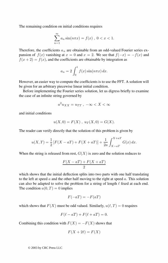
Results are shown below for a string which was deßected initially in a squarewave. The example was chosen to illustrate the approximation produced when asmall number of Fourier coefÞcients, in this case 30, is used. Ripples are clearlyevident in the surface plot of u(x, t) in Figure 9.5. The deßection conÞguration of


0 0.1 0.2 0.3 0.4 0.5 0.6 0.7 0.8 0.9 10

0.5

1

−1.5

−1

−0.5

0

0.5

1

1.5 String Deflection as a Function of Position and Time

x axis

tran

sver

se d

efle

ctio

n

time axis

Figure 9.5: String Deßection as a Function of Position and Time

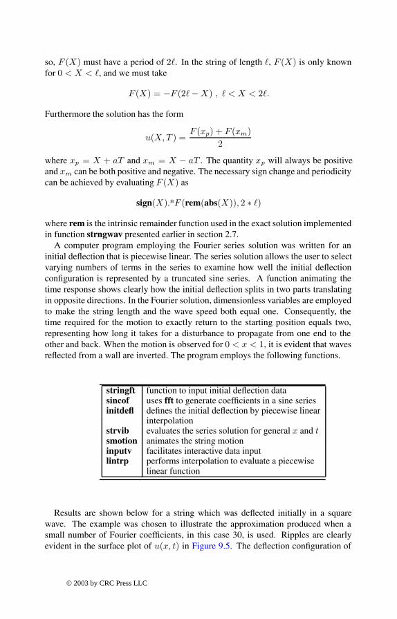
the string at t = 1 when the initial deßection form has passed through half a periodof motion appears in Figure 9.6. One other example given in Figure 9.7 shows thedeßection surface produced using 100 series terms and a triangular initial deßectionpattern. The surface describes u(x, t) through one period of motion.


Wave Propagation in a String

Figure 9.6: Wave Propagation in a String

00.2

0.40.6

0.81

0

0.5

1

1.5

2−1

−0.5

0

0.5

1

x axis

String Deflection as a Function of Position and Time

time axis

tran

sver

se d

efle

ctio

n

Figure 9.7: Surface for Triangular Initial Deßection


Program Output and Code

Output from Example stringft

>> stringft;

FOURIER SERIES SOLUTION FOR WAVESIN A STRING WITH LINEARLY INTERPOLATED

INITIAL DEFLECTION AND FIXED ENDS

Enter the number of interior data points (the fixedend point coordinates are added automatically)? 4

The string stretches between fixed endpoints atx=zero and x=one.

Enter 4 sets of x,y to specify interiorinitial deflections (one pair per line)

? .33,0? .33,-1? .67,-1? .67,0

Give the number of series termsand the maximum value of t(give 0,0 to stop)? 30,1

Press [Enter] tosee the animation

Give the number of series termsand the maximum value of t(give 0,0 to stop)? 0,0

>>

String Vibration Program

1: function [x,t,y]=stringft(Xdat,Ydat)2: %


3: % Example: [x,t,y]=stringft(Xdat,Ydat)4: % ~~~~~~~~~~~~~~~5: % This program analyzes wave motion in a string6: % having arbitrary piecewise linear initial7: % deflection. A Fourier series expansion is used8: % to construct the solution9: %

10: % Xdat,Ydat -data vectors defining the initial11: % deflections at interior points. The12: % deflections at x=0 and x=1 are set13: % to xero automatically. For example,14: % try Xdat=[.2,.3,.7,.8],15: % Ydat=[0,-1,-1,0]16: %17: % x,t,y - arrays containing the position, time18: % and deflection values19: %20: % User m functions required:21: % sincof, initdefl, strvib, smotion, inputv,22: % lintrp23:

24: global xdat ydat25:

26: disp(’ ’), disp( ...27: ’ FOURIER SERIES SOLUTION FOR WAVES’)28: disp(....29: ’IN A STRING WITH LINEARLY INTERPOLATED’)30: disp(...’31: ’ INITIAL DEFLECTION AND FIXED ENDS’)32: if nargin==033: disp(’ ’)34: disp([’Enter the number of interior ’,...35: ’data points (the fixed’])36: disp([’end point coordinates are ’,...37: ’added automatically)’])38: n=input(’? ’); if isempty(n), break, end39: xdat=zeros(n+2,1); ydat=xdat; xdat(n+2)=1;40: disp(’ ’)41: disp([’The string stretches between ’,...42: ’fixed endpoints at’])43: disp(’x=zero and x=one. ’),disp(’ ’)44: disp([’Enter ’,num2str(n),...45: ’ sets of x,y to specify interior’])46: disp([’initial deflections ’,...47: ’(one pair per line)’]), disp(’ ’)


48: for j=2:n+1,[xdat(j),ydat(j)]=inputv; end;49: else50: xdat=[0;Xdat(:);1]; ydat=[0;Ydat(:);0];51: end52:

53: a=sincof(@initdefl,1,1024); % sine coefficients54: nx=51; x=linspace(0,1,nx);55: xx=linspace(0,1,151);56:

57: while 158: disp(’ ’)59: disp(’Give the number of series terms’)60: disp(’and the maximum value of t’)61: disp(’(give 0,0 to stop)’)62: [ntrms,tmax]=inputv;63: if isnan(ntrms)| norm([ntrms,tmax])==064: break, end65: nt=ceil(nx*tmax); t=linspace(0,tmax,nt);66: y=strvib(a,t,x,1,ntrms); % time history67: yy=strvib(a,t,xx,1,ntrms);68: [xo,to]=meshgrid(x,t);69: hold off; surf(xo,to,y);70: grid on; colormap([1 1 1]);71: %colormap([127/255 1 212/255]);72: xlabel(’x axis’); ylabel(’time axis’);73: zlabel(’transverse deflection’);74: title([’String Deflection as a Function ’, ...75: ’of Position and Time’]);76: disp(’ ’), disp(’Press [Enter] to’)77: disp(’see the animation’), shg, pause78: % print -deps strdefl79: smotion(xx,yy,’Wave Propagation in a String’);80: disp(’’); pause(1);81: end82: % print -deps strwave83:

84: %=============================================85:

86: function y=initdefl(x)87: %88: % y=initdefl(x)89: % ~~~~~~~~~~~~~90: % This function defines the linearly91: % interpolated initial deflection92: % configuration.


93: %94: % x - a vector of points at which the initial95: % deflection is to be computed96: %97: % y - transverse initial deflection value for98: % argument x99: %

100: % xdat, ydat - global data vectors used for101: % linear interpolation102: %103: % User m functions required: lintrp104: %----------------------------------------------105:

106: global xdat ydat107: y=lintrp(xdat,ydat,x);108:

109: %=============================================110:

111: function y=strvib(a,t,x,hp,n)112: %113: % y=strvib(a,t,x,hp,n)114: % ~~~~~~~~~~~~~~~~~~~~115: % Sum the Fourier series for the string motion.116: %117: % a - Fourier coefficients of initial118: % deflection119: % t,x - vectors of time and position values120: % hp - the half period for the series121: % expansion122: % n - the number of series terms used123: %124: % y - matrix with y(i,j) equal to the125: % deflection at position x(i) and126: % time t(j)127: %128: % User m functions required: none129: %----------------------------------------------130:

131: w=pi/hp*(1:n); a=a(1:n); a=a(:)’;132: x=x(:); t=t(:)’;133: y=((a(ones(length(x),1),:).* ...134: sin(x*w))*cos(w(:)*t))’;135:

136: %=============================================137:


138: function smotion(x,y,titl)139: %140: % smotion(x,y,titl)141: % ~~~~~~~~~~~~~~~~~142: % This function animates the string motion.143: %144: % x - a vector of position values along the145: % string146: % y - a matrix of transverse deflection147: % values where successive rows give148: % deflections at successive times149: % titl - a title shown on the plot (optional)150: %151: % User m functions required: none152: %----------------------------------------------153:

154: if nargin < 3, titl=’ ’; end155: xmin=min(x); xmax=max(x);156: ymin=min(y(:)); ymax=max(y(:));157: [nt,nx]=size(y); clf reset;158: for j=1:nt159: plot(x,y(j,:),’k’);160: axis([xmin,xmax,2*ymin,2*ymax]);161: axis(’off’); title(titl);162: drawnow; figure(gcf); pause(.1)163: end164:

165: %=============================================166:

167: function a=sincof(func,hafper,nft)168: %169: % a=sincof(func,hafper,nft)170: % ~~~~~~~~~~~~~~~~~~~~~~~~~171: % This function calculates the sine172: % coefficients.173: %174: % func - the name of a function defined over175: % a half period176: % hafper - the length of the half period of the177: % function178: % nft - the number of function values used179: % in the Fourier series180: %181: % a - the vector of Fourier sine series182: % coefficients


183: %184: % User m functions required: none185: %----------------------------------------------186:

187: n2=nft/2; x=hafper/n2*(0:n2);188: y=feval(func,x); y=y(:);189: a=fft([y;-y(n2:-1:2)]); a=-imag(a(2:n2))/n2;190:

191: %=============================================192:

193: % function y=lintrp(xd,yd,x)194: % See Appendix B195:

196: %=============================================197:

198: % function varargout=inputv(prompt)199: % See Appendix B

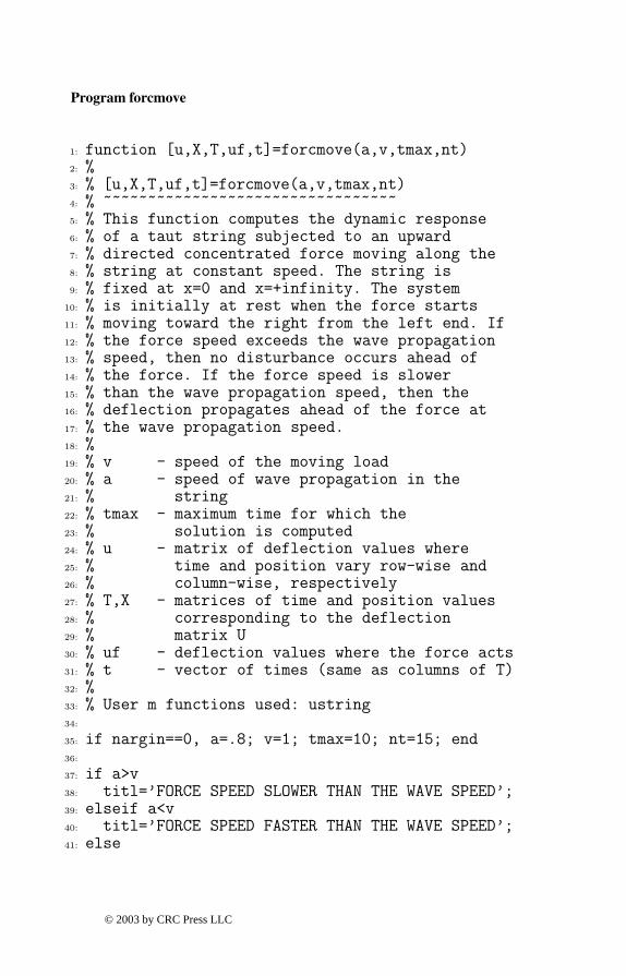
9.4 Force Moving on an Elastic String

The behavior of a semi-inÞnite string acted on by a moving transverse force illus-trates an interesting aspect of wave propagation. Consider a taut string initially atrest and un-deßected when a force moving at constant speed is applied. This simpleexample shows how a wave front moves ahead of the force when the velocity of wavepropagation in the string exceeds the speed of the force, but the force acts at the frontof the disturbance when the force moves faster than the wave speed of the string. Thegoverning differential equations, initial conditions, and boundary conditions are:

a2uxx(x, t) = utt(x, t) +F0

ρδ(x− vt) , t > 0 , 0 < x <∞,

u(0, t) = 0 , u(∞, t) = 0,

u(x, 0) = 0 , ut(x, 0) = 0 , 0 < x <∞.

In these equations a is the speed of wave propagation in the string and v is the speedat which a concentrated downward force F0 moves toward the right along the string,ρ is the mass per unit length of the string, and δ is the Dirac delta function. Thisproblem can be solved using the Fourier sine transform pair deÞned by

U(p, t) =

∞∫0

u(x, t) sin(px)dx , u(x, t) =2π

∞∫0

U(p, t) sin(px)dp.


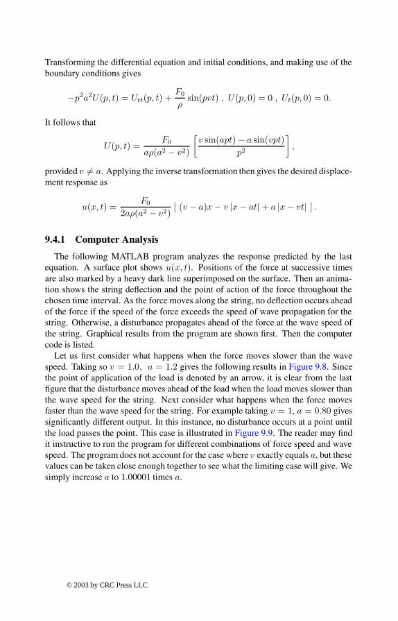
Transforming the differential equation and initial conditions, and making use of theboundary conditions gives

−p2a2U(p, t) = Utt(p, t) +F0

ρsin(pvt) , U(p, 0) = 0 , Ut(p, 0) = 0.

It follows that

U(p, t) =F0

aρ(a2 − v2)

[v sin(apt) − a sin(vpt)

p2

],

provided v = a. Applying the inverse transformation then gives the desired displace-ment response as

u(x, t) =F0

2aρ(a2 − v2)[ (v − a)x− v |x− at| + a |x− vt| ] .

9.4.1 Computer Analysis

The following MATLAB program analyzes the response predicted by the lastequation. A surface plot shows u(x, t). Positions of the force at successive timesare also marked by a heavy dark line superimposed on the surface. Then an anima-tion shows the string deßection and the point of action of the force throughout thechosen time interval. As the force moves along the string, no deßection occurs aheadof the force if the speed of the force exceeds the speed of wave propagation for thestring. Otherwise, a disturbance propagates ahead of the force at the wave speed ofthe string. Graphical results from the program are shown Þrst. Then the computercode is listed.

Let us Þrst consider what happens when the force moves slower than the wavespeed. Taking so v = 1.0, a = 1.2 gives the following results in Figure 9.8. Sincethe point of application of the load is denoted by an arrow, it is clear from the lastÞgure that the disturbance moves ahead of the load when the load moves slower thanthe wave speed for the string. Next consider what happens when the force movesfaster than the wave speed for the string. For example taking v = 1, a = 0.80 givessigniÞcantly different output. In this instance, no disturbance occurs at a point untilthe load passes the point. This case is illustrated in Figure 9.9. The reader may Þndit instructive to run the program for different combinations of force speed and wavespeed. The program does not account for the case where v exactly equals a, but thesevalues can be taken close enough together to see what the limiting case will give. Wesimply increase a to 1.00001 times a.


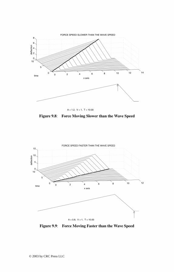
0 2 4 6 8 10 12 140

5

100

2

4

6

8FORCE SPEED SLOWER THAN THE WAVE SPEED

x axistime

defle

ctio

n

A = 1.2, V = 1, T = 10.00

Figure 9.8: Force Moving Slower than the Wave Speed

0 2 4 6 8 10 120

5

100

5

10

15FORCE SPEED FASTER THAN THE WAVE SPEED

x axistime

defle

ctio

n

A = 0.8, V = 1, T = 10.00

Figure 9.9: Force Moving Faster than the Wave Speed


Program forcmove

1: function [u,X,T,uf,t]=forcmove(a,v,tmax,nt)2: %3: % [u,X,T,uf,t]=forcmove(a,v,tmax,nt)4: % ~~~~~~~~~~~~~~~~~~~~~~~~~~~~~~~~~5: % This function computes the dynamic response6: % of a taut string subjected to an upward7: % directed concentrated force moving along the8: % string at constant speed. The string is9: % fixed at x=0 and x=+infinity. The system

10: % is initially at rest when the force starts11: % moving toward the right from the left end. If12: % the force speed exceeds the wave propagation13: % speed, then no disturbance occurs ahead of14: % the force. If the force speed is slower15: % than the wave propagation speed, then the16: % deflection propagates ahead of the force at17: % the wave propagation speed.18: %19: % v - speed of the moving load20: % a - speed of wave propagation in the21: % string22: % tmax - maximum time for which the23: % solution is computed24: % u - matrix of deflection values where25: % time and position vary row-wise and26: % column-wise, respectively27: % T,X - matrices of time and position values28: % corresponding to the deflection29: % matrix U30: % uf - deflection values where the force acts31: % t - vector of times (same as columns of T)32: %33: % User m functions used: ustring34:

35: if nargin==0, a=.8; v=1; tmax=10; nt=15; end36:

37: if a>v38: titl=’FORCE SPEED SLOWER THAN THE WAVE SPEED’;39: elseif a<v40: titl=’FORCE SPEED FASTER THAN THE WAVE SPEED’;41: else


42: titl=’FORCE SPEED EQUAL TO THE WAVE SPEED’;43: a=v*1.00001;44: end45:

46: % Obtain solution values and plot results47: [u,X,T,uf,t]=ustring(a,v,tmax,nt);48: if a>v, xf=X(:,2); uf=u(:,2); xw=X(:,3);49: else, xf=X(:,3); uf=u(:,3); end50: close, subplot(211)51: waterfall(X,T,-u), xlabel(’x axis’)52: ylabel(’time’), zlabel(’deflection’)53:

54: title(titl), grid on, hold on55: % plot3(xf,t,-uf,’.k’,xf,t,-uf,’k’)56: plot3(xf,t,-uf,’k’,’linewidth’,2);57: colormap([0 0 0]), view([-10,30]), shg58: umin=min(u(:)); umax=max(u(:)); xmax=X(1,4);59: range=[0,xmax,2*umin,2*umax]; hold on60: Titl=[’A = ’,num2str(a),’, V = ’,num2str(v),...61: ’, T = %4.2f’]; subplot(212) , axis off62:

63: % Use a dense set of points for animation64: nt=80; [uu,XX,TT,uuf,tt]=ustring(a,v,tmax,nt);65: umax=max(abs(uu(:))); uu=uu/umax; uuf=uuf/umax;66: XX=XX/xmax; range=[0,1,-1,1]; h=.4;67: arx=h*[0,.02,-.02,0,0]; ary=h*[0,.25,.25,0,1];68: for j=1:nt69: uj=uu(j,:); xj=XX(j,:);70: xfj=v/xmax*tt(j); ufj=uuf(j);71: plot(xj,-uj,’k’,xfj+arx,-ufj-ary,’-k’)72: axis off, time=(sprintf(Titl,tt(j)));73: text(.3,-.5,time), axis(range), drawnow74: pause(.05), figure(gcf), if j<nt, cla, end75: end76: % print -deps forcmove77: hold off; subplot78:

79: %=============================================80:

81: function [u,X,T,uf,t]=ustring(a,v,tmax,nt)82: %83: % [u,X,T,uf,t]=ustring(a,v,tmax,nt)84: % ~~~~~~~~~~~~~~~~~~~~~~~~~~~~~~~~85: % This function computes the deflection u(x,t)86: % of a semi-infinite string subjected to a


87: % moving force. The equation for the normalized88: % deflection is89: % u(x,t)=1/a/(a^2-v^2)*((v-a-v*abs(x-a*t)...90: % +a*abs(x-v*t));91: % a - speed of wave propagation in the string92: % v - speed of the force moving to the right93: % tmax - maximum time for computing the solution94: % nt - number of time values95: % uu - array of displacement values normalized96: % by dividing by a factor equal to the force97: % magnitude over twice the density per unit98: % length. Position varies column-wise and99: % time varies row-wise in the array.

100: % X,T - position and time arrays for the solution101: % uf - deflection vector under the force102: % t - time vector for the solution (same as the103: % columns of T)104: %105: t=linspace(0,tmax,nt)’; xmax=1.05*tmax*max(a,v);106: u=zeros(nt,4); nx=4; X=zeros(nt,nx); X(:,nx)=xmax;107: c=1/a/(a^2-v^2); xw=a*t; xf=v*t; T=repmat(t,1,4);108: uw=c*xw*(v-a+abs(v-a)); uf=c*xf*(v-a-abs(v-a));109: if a>v, X(:,2)=xf; X(:,3)=xw; u(:,2)=uf;110: else, X(:,2)=xw; X(:,3)=xf; u(:,2)=uw; end

9.5 Waves in Rectangular or Circular Membranes

Wave propagation in two dimensions is illustrated well by the transverse vibrationof an elastic membrane. Membrane dynamics is discussed here for general boundaryshapes. Then speciÞc solutions are given for rectangular and circular membranessubjected to a harmonically varying surface force. In the next chapter, natural modevibrations of an elliptical membrane are also discussed. We consider a membraneoccupying an area S of the x, y plane bounded by a curve L where the deßection iszero. The differential equation, boundary conditions, and initial conditions govern-ing the transverse deßection U(x, y, t) are

∇2U = c−2Utt − P (x, y, t) , (x, y) ∈ S,

U(x, y, 0) = U0(x, y) , Ut(x, y, 0) = V0(x, y) , (x, y) ∈ S,

U(x, y, t) = 0 , (x, y) ∈ L.

The parameter c is the speed of wave propagation in the membrane and P is theapplied normal load per unit area divided by the membrane tension per unit length.


When P = 0 , the motion is resolvable into a series of normal mode vibrations [22]of the form un(x, y) sin(Ωnt+ εn) satisfying

∇2un(x, y) = −Λ2n un(x, y), (x, y) ∈ S , un(x, y) = 0 , (x, y) ∈ L

where Λn = Ωn/c is a positive real frequency parameter, and un satisÞes∫∫un(x, y)um(x, y) dxdy = Cnδnm , Cn =

∫∫un(x, y)2dxdy

where δnm is the Kronecker delta symbol. If the initial displacement and initialvelocity are representable by a series of the modal functions, then the homogeneoussolution satisfying general initial conditions is

U(x, y, t) =∞∑

n=1

un(x, y) [An cos(Ωnt) +Bn sin(Ωnt)/Ωn]

where

An =∫∫

U0(x, y)un(x, y) dxdy/Cn , Bn =∫∫

V0(x, y)un(x, y) dxdy/Cn.

The nonhomogeneous case will be treated where the applied normal force on themembrane varies harmonically as

P (x, y, t) = p(x, y) cos(Ω t)

and Ω does not match any natural frequency of the membrane. We assume that themembrane is initially at rest with zero deßection and p(x, y) is expandable as

p(x, y) =∞∑

n=1

Pnun(x, y) dxdy , Pn =∫∫

p(x, y)un(x, y) dxdy/Cn.

Then the forced response solution satisfying zero initial conditions is found to be

U(x, y, t) =∞∑

n=1

Pn

Λ2 − Λ2n

un(x, y) [cos(Ω t) − cos(Ωnt)].

This equation shows clearly that when the frequency of the forcing function is closeto any one of the natural frequencies, then large deßection amplitudes can occur.

Next we turn to speciÞc solutions for rectangular and circular membranes. Con-sider the normal mode functions for a rectangular region deÞned by 0 ≤ x ≤ a,0 ≤ y ≤ b. It can be shown that the modal functions are

unm(x, y) = sin(nπx/a) sin(mπy/b) , Ωnm = cπ√

(n/a)2 + (m/b)2

and Cn = ab/4. In the simple case where the applied surface force is a concentratedload applied at (x0, y0), then

p(x, y) = p0δ(x− x0) δ(y − y0)


where δ is the Dirac delta function. The series solution for a forced response solutionis found to be

U(x, y, t) = c2∞∑

n=1

∞∑m=1

Pnm

Ω2 − Ω2nm

sin(nπx

a) sin(

mπy

b) [cos(Ω t) − cos(Ωnmt)]

with

Pnm =4p0

absin(nπx0/a) sin(mπy0/b).

A similar kind of solution is obtainable as a series of Bessel functions when themembrane is circular. Transforming the wave equation to polar coordinates (r, θ)gives

Urr + r−1Ur + r−2Uθθ = c−2Utt − P (r, θ, t) , 0 ≤ r ≤ a , −π ≤ θ ≤ π , t > 0.

To reduce the algebraic complexity of the series solution developed below, it is help-ful to introduce dimensionless variables ρ = r/a and τ = c t/a . Then the boundaryvalue problem involving a harmonic forcing function becomes

Uρρ+ρ−1Uρ+ρ−2Uθθ = Uττ−p(ρ, θ) sin(ω τ) , 0 ≤ ρ ≤ 1 , −π ≤ θ ≤ π , τ > 0,

U(ρ, θ, 0) = 0 , Uτ (ρ, θ, 0) = 0,

where ω = Ω a/c. The modal functions for this problem are

unm(ρ, θ) = Jn(λnmρ) cos(nθ + εn)

involving the integer order Bessel functions, with λnm being the mth positive root ofJn(ρ) . These modal functions satisfy the orthogonality conditions discussed aboveand we employ the series expansion

p(ρ, θ) =∞∑

n=0

∞∑m=1

Jn(λnmρ) real(Anmeinθ)

where

Anm =2

π(1 + δn0)J2n+1(λnm)

π∫−π

1∫0

p(ρ, θ)ρ Jn(λnmρ)e−inθdρ dθ.

Then the forced response solution becomes

U(ρ, θ, τ) =∞∑

n=0

∞∑m=1

Jn(λnmρ)ω2 − λ2

nm

real(Anmeinθ) [cos(ωτ) − cos(λnmτ)].

In the special case where a concentrated force acts at ρ = ρ0, θ = 0 , so that

p(ρ, θ) = p0δ(ρ− ρ0)δ(θ),

then evaluating the double integral gives

Anm = p0ρ0Jn(λnmρ0)

and real(Anme−inθ) simpliÞes to Anm cos(nθ).


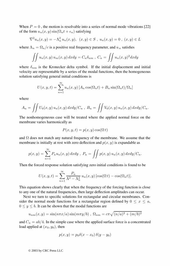
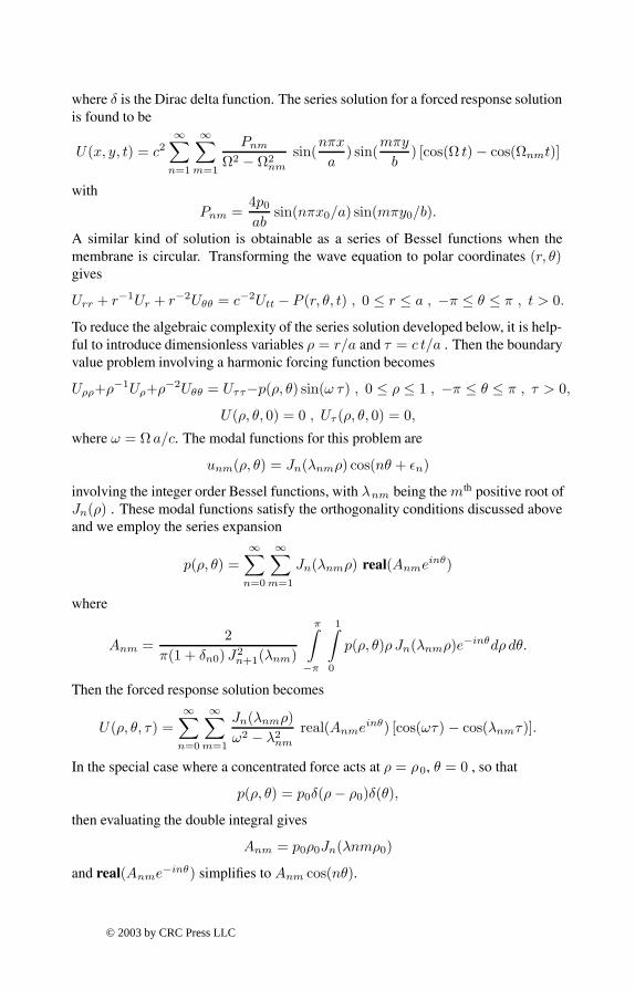
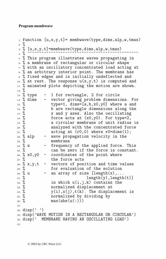
9.5.1 Computer Formulation

Program membwave was written to depict wave propagation in a rectangular orcircular membrane. Input data speciÞes information on membrane dimensions, forc-ing function frequency, force position coordinates, wave speed, and maximum timefor solution generation. The primary computation tasks involve summing the doubleseries deÞning the solutions. In the case of the circular membrane, the Bessel func-tion roots determining the natural frequencies must also be computed. The variousprogram modules are listed in the following table.

membwave reads data, calls other computational mod-ules, and outputs time response

memrecwv sums the series for dynamic response of arectangular membrane

memcirwv calls besjroot to obtain the natural frequen-cies and sums the series for the circular mem-brane response

besjroot computes a table of Bessel function rootsmembanim animates the dynamic response of the mem-

brane

9.5.2 Input Data for Program membwave

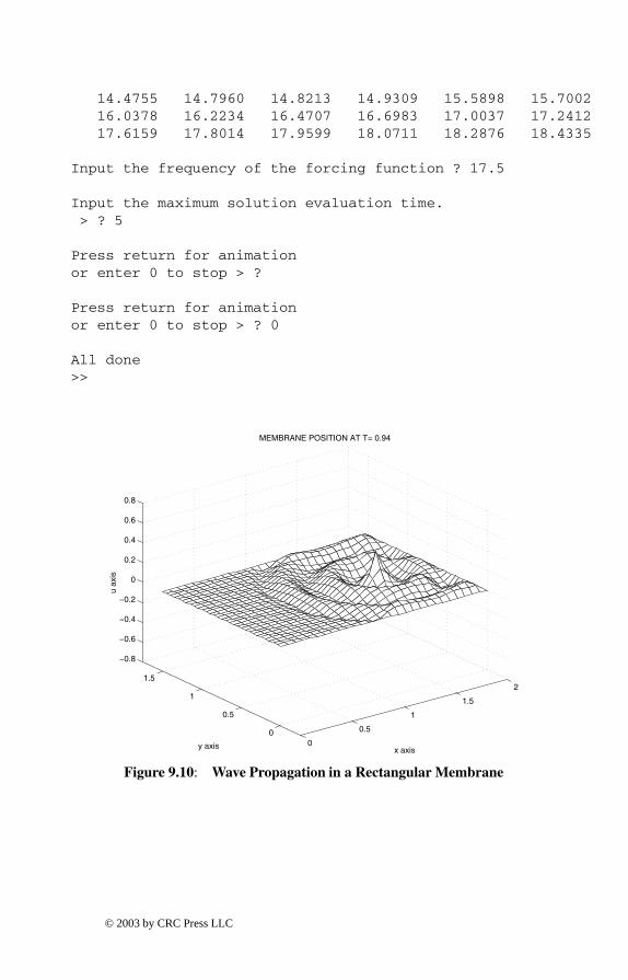
Listed below are data cases showing animations of both rectangular and circularmembranes. Waves propagate outward in a circular pattern from the point of appli-cation of the oscillating concentrated load. The membrane response becomes morecomplex as waves reßect from all parts of the boundary. In order to fully appreciatethe propagating wave phenomenon, readers should run the program for several com-binations of forcing function frequency and maximum time. The two surface plotsbelow show deßected positions before waves have reached the entire boundary, sosome parts of the membrane surface still remain undisturbed.

>> membwave;

WAVE MOTION IN A RECTANGULAR OR CIRCULARMEMBRANE HAVING AN OSCILLATING LOAD

Select the geometry type:Enter 1 for a rectangle, 2 for a circle > ? 1

Specify the rectangle dimensions:Give values for a,b > ? 2,1

Give coordinates (x0,y0) where the


force act. Enter x0,y0 > ? 1.5,.5

Enter the wave speed > ? 1

The first forty-two natural frequencies are:3.5124 4.4429 5.6636 6.4766 7.0248 7.02487.8540 8.4590 8.8858 9.5548 9.9346 9.9346

10.0580 10.5372 11.3272 11.3272 11.4356 12.268312.6642 12.6642 12.9531 12.9531 13.3286 13.420914.0496 14.0496 14.4820 14.4820 14.8189 15.470515.7080 15.7080 15.7863 16.0190 16.0190 16.399616.6978 16.9180 16.9180 16.9908 17.5620 17.5620

Input the frequency of the forcing function ? 17.5

Input the maximum solution evaluation time.> ? 5

Press return for animationor enter 0 to stop > ?

Press return for animationor enter 0 to stop > ? 0

All done

>> membwave;

WAVE MOTION IN A RECTANGULAR OR CIRCULARMEMBRANE HAVING AN OSCILLATING LOAD

Select the geoemtry type:Enter 1 for a rectangle, 2 for a circle > ? 2

The circle radius equals one. Give the radialdistance r0 from the circle center to theforce > ? .5

Enter the wave speed > ? 1

The first forty-two natural frequencies are:2.4048 3.8317 5.1356 5.5201 6.3801 7.01567.5883 8.4173 8.6537 8.7715 9.7611 9.9362

10.1735 11.0647 11.0864 11.6199 11.7916 12.225112.3385 13.0152 13.3237 13.3543 13.5893 14.3726


14.4755 14.7960 14.8213 14.9309 15.5898 15.700216.0378 16.2234 16.4707 16.6983 17.0037 17.241217.6159 17.8014 17.9599 18.0711 18.2876 18.4335

Input the frequency of the forcing function ? 17.5

Input the maximum solution evaluation time.> ? 5

Press return for animationor enter 0 to stop > ?

Press return for animationor enter 0 to stop > ? 0

All done>>

0

0.5

1

1.5

2

0

0.5

1

1.5

−0.8

−0.6

−0.4

−0.2

0

0.2

0.4

0.6

0.8

x axis

MEMBRANE POSITION AT T= 0.94

y axis

u ax

is

Figure 9.10: Wave Propagation in a Rectangular Membrane


−1

−0.5

0

0.5

1

−1

−0.5

0

0.5

1

−1

−0.5

0

0.5

1

x axis

MEMBRANE POSITION AT T= 0.96

y axis

u ax

is

Figure 9.11: Wave Propagation in a Circular Membrane


Program membwave

1: function [u,x,y,t]= membwave(type,dims,alp,w,tmax)2: %3: % [u,x,y,t]=membwave(type,dims,alp,w,tmax)4: % ~~~~~~~~~~~~~~~~~~~~~~~~~~~~~~~~~~~~~~~~~~~~~~~5: % This program illustrates waves propagating in6: % a membrane of rectangular or circular shape7: % with an oscillatory concentrated load acting at8: % an arbitrary interior point. The membrane has9: % fixed edges and is initially undeflected and

10: % at rest. The response u(x,y,t) is computed and11: % animated plots depicting the motion are shown.12: %13: % type - 1 for rectangle, 2 for circle14: % dims - vector giving problem dimensions. For15: % type=1, dims=[a,b,x0,y0] where a and16: % b are rectangle dimensions along the17: % x and y axes. Also the oscillating18: % force acts at (x0,y0). For type=2,19: % a circular membrane of unit radius is20: % analyzed with the concentrated force21: % acting at (r0,0) where r0=dims(1);22: % alp - wave propagation velocity in the23: % membrane24: % w - frequency of the applied force. This25: % can be zero if the force is constant.26: % x0,y0 - coordinates of the point where27: % the force acts28: % x,y,t - vectors of position and time values29: % for evaluation of the solution30: % u - an array of size [length(x),...31: % length(y),length(t)]32: % in which u(i,j,k) contains the33: % normalized displacement at34: % y(i),x(j),t(k). The displacement is35: % normalized by dividing by36: % max(abs(u(:)))37:

38: disp(’ ’)39: disp(’WAVE MOTION IN A RECTANGULAR OR CIRCULAR’)40: disp(’ MEMBRANE HAVING AN OSCILLATING LOAD’)41:


42: if nargin > 0 % Data passed through the call list43: % must specify: type, dims, alp, w, tmax44: % Typical values are: a=2; b=1; alp=1;45: % w=18.4; x0=1; y0=0.5; tmax=5;46: if type==147: a=dims(1); b=dims(2); x0=dims(3); y0=dims(4);48: [u,x,y,t]=memrecwv(a,b,alp,w,x0,y0,tmax);49: else50: r0=dims(1);51: end52: else % Interactive data input53:

54: disp(’ ’), disp(’Select the geometry type:’)55: type=input([’Enter 1 for a rectangle, ’,...56: ’2 for a circle > ? ’]);57: if type ==158: disp(’ ’)59: disp(’Specify the rectangle dimensions:’)60: s=input(’Give values for a,b > ? ’,’s’);61: s=eval([’[’,s,’]’]); a=s(1); b=s(2);62: disp(’ ’)63: disp(’Give coordinates (x0,y0) where the’)64: s=input(’force acts. Enter x0,y0 > ? ’,’s’);65: s=eval([’[’,s,’]’]); x0=s(1); y0=s(2);66: disp(’ ’), alp=input(’Enter the wave speed > ? ’);67:

68: N=40; M=40; pan=pi/a*(1:N)’; pbm=pi/b*(1:M);69: W=alp*sqrt(repmat(pan.^2,1,M)+repmat(pbm.^2,N,1));70: wsort=sort(W(:)); wsort=reshape(wsort(1:42),6,7)’;71: disp(’ ’)72: disp([’The first forty-two natural ’,...73: ’frequencies are:’])74: disp(wsort)75: w=input(...76: ’Input the frequency of the forcing function ? ’);77:

78: else79: disp(’ ’), disp(...80: ’The circle radius equals one. Give the radial’)81: disp(...82: ’distance r0 from the circle center to the’)83: r0=input(’force > ? ’);84:

85: disp(’ ’), alp=input(’Enter the wave speed > ? ’);86:


87: % First 42 Bessel function roots88: wsort=alp*[...89: 2.4048 3.8317 5.1356 5.5201 6.3801 7.015690: 7.5883 8.4173 8.6537 8.7715 9.7611 9.936291: 10.1735 11.0647 11.0864 11.6199 11.7916 12.225192: 12.3385 13.0152 13.3237 13.3543 13.5893 14.372693: 14.4755 14.7960 14.8213 14.9309 15.5898 15.700294: 16.0378 16.2234 16.4707 16.6983 17.0037 17.241295: 17.6159 17.8014 17.9599 18.0711 18.2876 18.4335];96:

97: disp(’ ’), disp([’The first forty-two ’,...98: ’natural frequencies are:’])99: disp(wsort)

100: w=input(...101: ’Input the frequency of the forcing function ? ’);102: end103: disp(’ ’)104: disp(’Input the maximum solution evaluation time.’)105: tmax=input(’ > ? ’);106: end107:

108: if type==1109: [u,x,y,t]=memrecwv(a,b,alp,w,x0,y0,tmax);110: else111: th=linspace(0,2*pi,81); r=linspace(0,1,20);112: [u,x,y,t]=memcirwv(r,th,r0,alp,w,tmax);113: end114:

115: % Animate the solution116: membanim(u,x,y,t);117:

118: %================================================119:

120: function [u,x,y,t]= memrecwv(a,b,alp,w,x0,y0,tmax)121: %122: % [u,x,y,t]=memrecwv(a,b,alp,w,x0,y0,tmax)123: % ~~~~~~~~~~~~~~~~~~~~~~~~~~~~~~~~~~~~~~~124: % This function illustrates wave motion in a125: % rectangular membrane subjected to a concentrated126: % oscillatory force applied at an arbitrary127: % interior point. The membrane has fixed edges128: % and is initially at rest in an undeflected129: % position. The resulting response u(x,y,t)is130: % computed and a plot of the motion is shown.131: % a,b - side dimensions of the rectangle


132: % alp - wave propagation velocity in the133: % membrane134: % w - frequency of the applied force. This135: % can be zero if the force is constant.136: % x0,y0 - coordinates of the point where137: % the force acts138: % x,y,t - vectors of position and time values139: % for evaluation of the solution140: % u - an array of size [length(y),...141: % length(x),length(t)] in which u(i,j,k)142: % contains the normalized displacement143: % corresponding to y(i), x(j), t(k). The144: % displacement is normalized by dividing145: % by max(abs(u(:))).146: %147: % The solution is a double Fourier series of form148: %149: % u(x,y,t)=Sum(A(n,m,x,y,t), n=1..N, m=1..M)150: % where151: % A(n,m,x,y,t)=sin(n*pi*x0/a)*sin(n*pi*x/a)*...152: % sin(m*pi*y0/b)*sin(m*pi*y/b)*...153: % (cos(w*t)-cos(W(n,m)*t))/...154: % ( w^2-W(n,m)^2)155: % and the membrane natural frequencies are156: % W(n,m)=pi*alp*sqrt((n/a)^2+(m/b)^2)157:

158: if nargin==0159: a=2; b=1; alp=1; tmax=3; w=13; x0=1.5; y0=0.5;160: end161: if a<b162: nx=31; ny=round(b/a*21); ny=ny+rem(ny+1,2);163: else164: ny=31; nx=round(a/b*21); nx=nx+rem(nx+1,2);165: end166: x=linspace(0,a,nx); y=linspace(0,b,ny);167:

168: N=40; M=40; pan=pi/a*(1:N)’; pbm=pi/b*(1:M);169: W=alp*sqrt(repmat(pan.^2,1,M)+repmat(pbm.^2,N,1));170: wsort=sort(W(:)); wsort=reshape(wsort(1:30),5,6)’;171: Nt=ceil(40*tmax*alp/min(a,b));172: t=tmax/(Nt-1)*(0:Nt-1);173:

174: % Evaluate fixed terms in the series solution175: mat=sin(x0*pan)*sin(y0*pbm)./(w^2-W.^2);176: sxn=sin(x(:)*pan’); smy=sin(pbm’*y(:)’);


177:

178: u=zeros(ny,nx,Nt);179: for j=1:Nt180: A=mat.*(cos(w*t(j))-cos(W*t(j)));181: uj=sxn*(A*smy); u(:,:,j)=uj’;182: end183:

184: %================================================185:

186: function [u,x,y,t,r,th]=memcirwv(r,th,r0,alp,w,tmax)187: %188: % [u,x,y,t,r,th]=memcirwv(r,th,r0,alp,w,tmax)189: % ~~~~~~~~~~~~~~~~~~~~~~~~~~~~~~~~~~~~~~~~~~190: % This function computes the wave response in a191: % circular membrane having an oscillating force192: % applied at a point on the radius along the193: % positive x axis.194: %195: % r,th - vectors of radius and polar angle values196: % r0 - radial position of the concentrated force197: % w - frequency of the applied force198: % tmax - maximum time for computing the solution199: %200: % User m function used: besjroot201:

202: if nargin==0203: r0=.4; w=15.5; th=linspace(0,2*pi,81);204: r=linspace(0,1,21); alp=1;205: end206:

207: Nt=ceil(20*alp*tmax); t=tmax/(Nt-1)*(0:Nt-1);208:

209: % Compute the Bessel function roots needed in210: % the series solution. This takes a while.211: lam=besjroot(0:20,20,1e-3);212:

213: % Compute the series coefficients214: [nj,nk]=size(lam); r=r(:)’; nr=length(r);215: th=th(:); nth=length(th); nt=length(t);216: N=repmat((0:nj-1)’,1,nk); Nvec=N(:)’;217: c=besselj(N,lam*r0)./(besselj(...218: N+1,lam).^2.*(lam.^2-w^2));219: c(1,:)=c(1,:)/2; c=c(:)’;220:

221: % Sum the series of Bessel functions


222: lamvec=lam(:)’; wlam=w./lamvec;223: c=cos(th*Nvec).*repmat(c,nth,1);224: rmat=besselj(repmat(Nvec’,1,nr),lamvec’*r);225: u=zeros(nth,nr,nt);226: for k=1:nt227: tvec=-cos(w*t(k))+cos(lamvec*t(k));228: u(:,:,k)=c.*repmat(tvec,nth,1)*rmat;229: end230: u=2/pi*u; x=cos(th)*r; y=sin(th)*r;231:

232: %================================================233:

234: function rts=besjroot(norder,nrts,tol)235: %236: % rts=besjroot(norder,nrts,tol)237: % ~~~~~~~~~~~~~~~~~~~~~~~~~~~~238: % This function computes an array of positive roots239: % of the integer order Bessel functions besselj of240: % the first kind for various orders. A chosen number241: % of roots is computed for each order242: % norder - a vector of function orders for which243: % roots are to be computed. Taking 3:5244: % for norder would use orders 3,4 and 5.245: % nrts - the number of positive roots computed for246: % each order. Roots at x=0 are ignored.247: % rts - an array of roots having length(norder)248: % rows and nrts columns. The element in249: % column k and row i is the k’th root of250: % the function besselj(norder(i),x).251: % tol - error tolerance for root computation.252:

253: if nargin<3, tol=1e-5; end254: jn=inline(’besselj(n,x)’,’x’,’n’);255: N=length(norder); rts=ones(N,nrts)*nan;256: opt=optimset(’TolFun’,tol,’TolX’,tol);257: for k=1:N258: n=norder(k); xmax=1.25*pi*(nrts-1/4+n/2);259: xsrch=.1:pi/4:xmax; fb=besselj(n,xsrch);260: nf=length(fb); K=find(fb(1:nf-1).*fb(2:nf)<=0);261: if length(K)<nrts262: disp(’Search error in function besjroot’)263: rts=nan; return264: else265: K=K(1:nrts);266: for i=1:nrts


267: interval=xsrch(K(i):K(i)+1);268: rts(k,i)=fzero(jn,interval,opt,n);269: end270: end271: end272:

273: %================================================274:

275: function membanim(u,x,y,t)276: %277: % function membanim(u,x,y,t)278: % ~~~~~~~~~~~~~~~~~~~~~~~~~279: % This function animates the motion of a280: % vibrating membrane281: %282: % u array in which component u(i,j,k) is the283: % displacement for y(i),x(j),t(k)284: % x,y arrays of x and y coordinates285: % t vector of time values286:

287: % Compute the plot range288: if nargin==0;289: [u,x,y,t]=memrecwv(2,1,1,15.5,1.5,.5,5);290: end291: xmin=min(x(:)); xmax=max(x(:));292: ymin=min(y(:)); ymax=max(y(:));293: xmid=(xmin+xmax)/2; ymid=(ymin+ymax)/2;294: d=max(xmax-xmin,ymax-ymin)/2; Nt=length(t);295: range=[xmid-d,xmid+d,ymid-d,ymid+d,...296: 3*min(u(:)),3*max(u(:))];297:

298: while 1 % Show the animation repeatedly299: disp(’ ’), disp(’Press return for animation’)300: dumy=input(’or enter 0 to stop > ? ’,’s’);301: if ~isempty(dumy)302: disp(’ ’), disp(’All done’), break303: end304:

305: % Plot positions for successive times306: for j=1:Nt307: surf(x,y,u(:,:,j)), axis(range)308: xlabel(’x axis’), ylabel(’y axis’)309: zlabel(’u axis’), titl=sprintf(...310: ’MEMBRANE POSITION AT T=%5.2f’,t(j));311: title(titl), colormap([1 1 1])


312: colormap([127/255 1 212/255])313: % axis off314: drawnow, shg, pause(.1)315: end316: end

9.6 Wave Propagation in a Beam with an ImpactMoment Applied to One End

Analyzing the dynamic response caused when a time dependent moment acts onthe end of an Euler beam involves a boundary value problem for a fourth order linearpartial differential equation. In the following example we consider a beam of uniformcross section which is pin-ended (hinged at the ends) and is initially at rest. Suddenly,a harmonically varying momentM0 cos(Ω0T ) is applied to the right end as shown inFigure 9.12. Determination of the resulting displacement and bending moment in thebeam is desired. Let U be the transverse displacement, X the longitudinal distance

E, I, L

M0cos(Ω0T)

Figure 9.12: Beam Geometry and Loading

from the right end, and T the time. The differential equation, boundary conditions,and initial conditions characterizing the problem are

EI∂4U

∂X4= −Aρ∂

2U

∂T 2, 0 < X < L , T > 0,

U(0, T ) = 0 ,∂2U

∂X2(0, T ) = 0 , U(L, T ) = 0 ,

∂2U

∂X2(L, T ) = M0 cos(Ω0T )/(EI),

U(0, T ) = 0 ,∂U

∂T(0, T ) = 0,

where L is the beam length,EI is the product of the elastic modulus and the momentof inertia, and Aρ is the product of the cross section area and the mass density.

This problem can be represented more conveniently by introducing dimensionlessvariables

x =X

L, t =

√EI

Aρ

T

L2, u =

EI

M0L2U , ω =

√Aρ

EIL2Ω0 , m =

∂2u

∂x2.


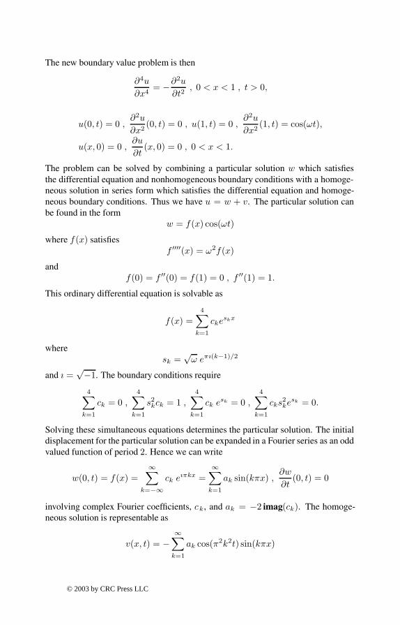
The new boundary value problem is then

∂4u

∂x4= −∂

2u

∂t2, 0 < x < 1 , t > 0,

u(0, t) = 0 ,∂2u

∂x2(0, t) = 0 , u(1, t) = 0 ,

∂2u

∂x2(1, t) = cos(ωt),

u(x, 0) = 0 ,∂u

∂t(x, 0) = 0 , 0 < x < 1.

The problem can be solved by combining a particular solution w which satisÞesthe differential equation and nonhomogeneous boundary conditions with a homoge-neous solution in series form which satisÞes the differential equation and homoge-neous boundary conditions. Thus we have u = w + v. The particular solution canbe found in the form

w = f(x) cos(ωt)

where f(x) satisÞesf ′′′′(x) = ω2f(x)

andf(0) = f ′′(0) = f(1) = 0 , f ′′(1) = 1.

This ordinary differential equation is solvable as

f(x) =4∑

k=1

ckeskx

wheresk =

√ω eπı(k−1)/2

and ı =√−1. The boundary conditions require

4∑k=1

ck = 0 ,4∑

k=1

s2kck = 1 ,4∑

k=1

ck esk = 0 ,

4∑k=1

cks2ke

sk = 0.

Solving these simultaneous equations determines the particular solution. The initialdisplacement for the particular solution can be expanded in a Fourier series as an oddvalued function of period 2. Hence we can write

w(0, t) = f(x) =∞∑

k=−∞ck e

ıπkx =∞∑

k=1

ak sin(kπx) ,∂w

∂t(0, t) = 0

involving complex Fourier coefÞcients, ck, and ak = −2 imag(ck). The homoge-neous solution is representable as

v(x, t) = −∞∑

k=1

ak cos(π2k2t) sin(kπx)


so that w + v combine to satisfy the desired initial conditions of zero displacementand velocity.

Of course, perfect satisfaction of the initial conditions cannot be achieved with-out taking an inÞnite number of terms in the Fourier series. However, the seriesconverges very rapidly because the coefÞcients are of order n−3. When a hundredor more terms are used, an approximate solution produces results which satisfy thedifferential equation and boundary conditions, and which insigniÞcantly violate theinitial displacement condition. It is important to remember the nature of this er-ror when examining the bending moment results presented below. Effects of highfrequency components are very evident in the moment. Despite the oscillatory char-acter of the moments, these results are exact for the initial displacement conditionsproduced by the truncated series. These displacements agree closely with the exactsolution.

A program was written to evaluate the series solution to compute displacementsand moments as functions of position and time. Plots and surfaces showing thesequantities are presented along with timewise animations of the displacement andmoment across the span. The computation involves the following steps:

1. Evaluate f(x);

2. Expand f(x) using the FFT to get coefÞcients for the homogeneous seriessolution;

3. Combine the particular and homogeneous solution by summing the series forany number of terms desired by the user;

4. Plot u and m for selected times;

5. Plot surfaces showing u(x, t) and m(x, t);

6. Show animated plots of u and m.

The principal parts of the program are shown in the table below.

bemimpac reads data and creates graphical outputbeamresp converts material property data to dimension-

less form and calls ndbemrspndbemrsp construct the solution using Fourier seriessumser sums the series for displacement and momentanimate animates the time history of displacement and

moment

The numerical results show the response for a beam subjected to a moment closeto the Þrst natural frequency of the beam. It can be shown that, in the dimensionlessproblem, the system of equations deÞning the particular solution becomes singular


0 0.1 0.2 0.3 0.4 0.5 0.6 0.7 0.8 0.9 1−0.07

−0.06

−0.05

−0.04

−0.03

−0.02

−0.01

0

0.01

0.02

0.03

x axis

disp

lace

men

t

Displacement for Nearly Resonant Moment Acting at Right End

Number of series terms used = 200

t=0.10t=0.20t=0.35

Figure 9.13: Displacement Due to Impact Moment at Right End

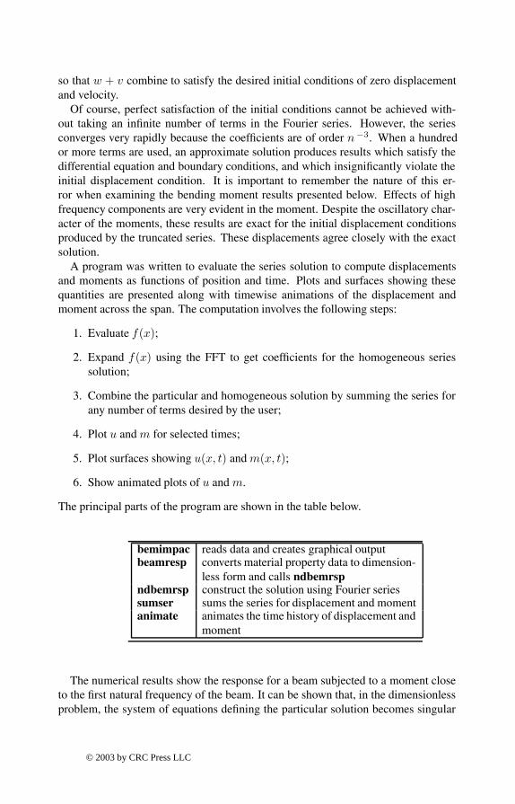
when ω assumes values of the form k2π2 for integer k. In that instance the seriessolution provided here will fail. However, values of ω near to resonance can be usedto show how the displacements and moments quickly become large. In our examplewe let EI , Aρ, l, and M0 all equal unity, and ω = 0.95π2. Figures 9.13 and 9.14show displacement and bending moment patterns shortly after motion is initiated.The surfaces in Figures 9.15 and 9.16 also show how the displacement and momentgrow quickly with increasing time. The reader may Þnd it interesting to run theprogram for various choices of ω and observe how dramatically the chosen forcingfrequency affects results.


0 0.1 0.2 0.3 0.4 0.5 0.6 0.7 0.8 0.9 1−1.5

−1

−0.5

0

0.5

1

1.5

x axis

mom

ent

Bending Moment for Nearly Resonant Moment Acting at Right End

Number of series terms used = 200

t=0.10t=0.20t=0.35

Figure 9.14: Bending Moment in the Beam

00.2

0.40.6

0.81

0

1

2

3

4−0.8

−0.6

−0.4

−0.2

0

0.2

0.4

0.6

0.8

x axis

Transverse Deflection as a Function of Time and Position

time

tran

sver

se d

efle

ctio

n

Figure 9.15: Displacement Growth Near Resonance


00.2

0.40.6

0.81

0

1

2

3

4−8

−6

−4

−2

0

2

4

6

8

x axis

Bending Moment as a Function of Time and Position

time

bend

ing

mom

ent

Figure 9.16: Moment Growth Near Resonance

MATLAB Example

Program bemimpac

1: function bemimpac2: % Example: bemimpac3: % ~~~~~~~~~~~~~~~~~4: % This program analyzes an impact dynamics5: % problem for an elastic Euler beam of6: % constant cross section which is simply7: % supported at each end. The beam is initially8: % at rest when a harmonically varying moment9: % m0*cos(w0*t) is applied to the right end.

10: % The resulting transverse displacement and11: % bending moment are computed. The12: % displacement and moment are plotted as13: % functions of x for the three time values.14: % Animated plots of the entire displacement15: % and moment history are also given.16: %17: % User m functions required:


18: % beamresp, beamanim, sumser, ndbemrsp19:

20: fprintf(’\nDYNAMICS OF A BEAM WITH AN ’);21: fprintf(’OSCILLATING END MOMENT\n’);22: ei=1; arho=1; len=1; m0=1; w0=.90*pi^2;23: tmin=0; tmax=5; nt=101;24: xmin=0; xmax=len; nx=151; ntrms=200;25: [t,x,displ,mom]=beamresp(ei,arho,len,m0,w0,...26: tmin,tmax,nt,xmin,xmax,nx,ntrms);27: disp(’ ’)28: disp(’Press [Enter] to see the deflection’)29: disp(’for three positions’), pause30:

31: np=[3 5 8]; clf; pltsave=0;32: dip=displ(np,:); mop=mom(np,:);33: plot(x,dip(1,:),’-k’,x,dip(2,:),’:b’,...34: x,dip(3,:),’--r’);35: xlabel(’x axis’); ylabel(’displacement’);36: hh=gca;37: r(1:2)=get(hh,’XLim’); r(3:4)=get(hh,’YLim’);38: xp=r(1)+(r(2)-r(1))/10;39: dp=r(4)-(r(4)-r(3))/10;40: tstr=[’Displacement for Nearly Resonant’ ...41: ’ Moment Acting at Right End’];42: title(tstr);43: text(xp,dp,[’Number of series terms ’ ...44: ’used = ’,int2str(ntrms)]);45: legend(’t=0.10’,’t=0.20’,’t=0.35’,3)46: disp(’ ’)47: disp(’Press [Enter] to the bending moment’)48: disp(’for three positions’)49: shg; pause50: if pltsave, print -deps 3positns, end51:

52: clf;53: plot(x,mop(1,:),’-k’,x,mop(2,:),’:b’,...54: x,mop(3,:),’--r’);55: h=gca;56: r(1:2)=get(h,’XLim’); r(3:4)=get(h,’YLim’);57: mp=r(3)+(r(4)-r(3))/10;58: xlabel(’x axis’); ylabel(’moment’);59: tstr=[’Bending Moment for Nearly Resonant’ ...60: ’ Moment Acting at Right End’];61: title(tstr);62: text(xp,mp,[’Number of series terms ’ ...


63: ’used = ’,int2str(ntrms)]);64: legend(’t=0.10’,’t=0.20’,’t=0.35’,2),65: disp(’ ’), disp(...66: ’Press [Enter] to see the deflections surface’)67: shg, pause68: if pltsave, print -deps 3moments, end69:

70: inct=2; incx=2;71: ht=0.75; it=1:inct:.8*nt; ix=1:incx:nx;72: tt=t(it); xx=x(ix);73: dd=displ(it,ix); mm=mom(it,ix);74: a=surf(xx,tt,dd);75: tstr=[’Transverse Deflection as a ’ ...76: ’Function of Time and Position’];77: title(tstr);78: xlabel(’x axis’); ylabel(’time’);79: zlabel(’transverse deflection’);80: disp(’ ’), disp([’Press [Enter] to ’,...81: ’see the bending moment surface’])82: shg, pause83: if pltsave, print -deps bdeflsrf, end84:

85: a=surf(xx,tt,mm);86: title([’Bending Moment as a Function ’ ...87: ’of Time and Position’])88: xlabel(’x axis’); ylabel(’time’);89: zlabel(’bending moment’); disp(’ ’)90: disp(’Press [Enter] to see animation of’);91: disp(’the beam deflection’), shg, pause92: if pltsave, print -deps bmomsrf, end93: beamanim(x,displ,.1,’Transverse Deflection’, ...94: ’x axis’,’deflection’), disp(’ ’)95: disp(’Press [Enter] to see animation’);96: disp(’of the bending moment’); pause97: beamanim(x,mom,.1,’Bending Moment History’, ...98: ’x axis’,’moment’);99: fprintf(’\nAll Done\n’); close;

100:

101: %=============================================102:

103: function [t,x,displ,mom]= ...104: beamresp(ei,arho,len,m0,w0,tmin,tmax, ...105: nt,xmin,xmax,nx,ntrms)106: %107: % [t,x,displ,mom]=beamresp(ei,arho,len,m0, ...


108: % w0,tmin,tmax,nt,xmin,xmax,nx,ntrms)109: % ~~~~~~~~~~~~~~~~~~~~~~~~~~~~~~~~~~~~~~~~~~~~~110: % This function evaluates the time dependent111: % displacement and moment in a constant112: % cross section, simply supported beam which113: % is initially at rest when a harmonically114: % varying moment is suddenly applied at the115: % right end. The resulting time histories of116: % displacement and moment are computed.117: %118: % ei - modulus of elasticity times119: % moment of inertia120: % arho - mass per unit length of the121: % beam122: % len - beam length123: % m0,w0 - amplitude and frequency of the124: % harmonically varying right end125: % moment126: % tmin,tmax - minimum and maximum times for127: % the solution128: % nt - number of evenly spaced129: % solution times130: % xmin,xmax - minimum and maximum position131: % coordinates for the solution.132: % These values should lie between133: % zero and len (x=0 and x=len at134: % the left and right ends).135: % nx - number of evenly spaced solution136: % positions137: % ntrms - number of terms used in the138: % Fourier sine series139: % t - vector of nt equally spaced time140: % values varying from tmin to tmax141: % x - vector of nx equally spaced142: % position values varying from143: % xmin to xmax144: % displ - matrix of transverse145: % displacements with time varying146: % from row to row, and position147: % varying from column to column148: % mom - matrix of bending moments with149: % time varying from row to row,150: % and position varying from column151: % to column152: %


153: % User m functions called: ndbemrsp154: %----------------------------------------------155:

156: tcof=sqrt(arho/ei)*len^2; dcof=m0*len^2/ei;157: tmin=tmin/tcof; tmax=tmax/tcof; w=w0*tcof;158: xmin=xmin/len; xmax=xmax/len;159: [t,x,displ,mom]=...160: ndbemrsp(w,tmin,tmax,nt,xmin,xmax,nx,ntrms);161: t=t*tcof; x=x*len;162: displ=displ*dcof; mom=mom*m0;163:

164: %=============================================165:

166: function beamanim(x,u,tpause,titl,xlabl,ylabl)167: %168: % beamanim(x,u,tpause,titl,xlabl,ylabl,save)169: % ~~~~~~~~~~~~~~~~~~~~~~~~~~~~~~~~~~~~170: % This function draws an animated plot of data171: % values stored in array u. The different172: % columns of u correspond to position values173: % in vector x. The successive rows of u174: % correspond to different times. Parameter175: % tpause controls the speed of animation.176: %177: % u - matrix of values to animate plots178: % of u versus x179: % x - spatial positions for different180: % columns of u181: % tpause - clock seconds between output of182: % frames. The default is .1 secs183: % when tpause is left out. When184: % tpause=0, a new frame appears185: % when the user presses any key.186: % titl - graph title187: % xlabl - label for horizontal axis188: % ylabl - label for vertical axis189: %190: % User m functions called: none191: %----------------------------------------------192:

193: if nargin<6, ylabl=’’; end;194: if nargin<5, xlabl=’’; end195: if nargin<4, titl=’’; end;196: if nargin<3, tpause=.1; end;197:


198: [ntime,nxpts]=size(u);199: umin=min(u(:)); umax=max(u(:));200: udif=umax-umin; uavg=.5*(umin+umax);201: xmin=min(x); xmax=max(x);202: xdif=xmax-xmin; xavg=.5*(xmin+xmax);203: xwmin=xavg-.55*xdif; xwmax=xavg+.55*xdif;204: uwmin=uavg-.55*udif; uwmax=uavg+.55*udif; clf;205: axis([xwmin,xwmax,uwmin,uwmax]); title(titl);206: xlabel(xlabl); ylabel(ylabl); hold on;207:

208: for j=1:ntime209: ut=u(j,:);210: plot(x,ut,’-’); axis(’off’); figure(gcf);211: if tpause==0212: pause;213: else214: pause(tpause);215: end216: if j==ntime, break, else, cla; end217: end218: % print -deps cntltrac219: hold off; clf;220:

221: %=============================================222:

223: function [u,t,x] = sumser(a,b,c,funt,funx, ...224: tmin,tmax,nt,xmin,xmax,nx)225: %226: % [u,t,x] = sumser(a,b,c,funt,funx,tmin, ...227: % tmax,nt,xmin,xmax,nx)228: % ~~~~~~~~~~~~~~~~~~~~~~~~~~~~~~~~~~~~~~~~~~229: % This function evaluates a function U(t,x)230: % which is defined by a finite series. The231: % series is evaluated for t and x values taken232: % on a rectangular grid network. The matrix u233: % has elements specified by the following234: % series summation:235: %236: % u(i,j) = sum( a(k)*funt(t(i)*b(k))*...237: % k=1:nsum238: % funx(c(k)*x(j))239: %240: % where nsum is the length of each of the241: % vectors a, b, and c.242: %


243: % a,b,c - vectors of coefficients in244: % the series245: % funt,funx - handles of functions accepting246: % matrix argument. funt is247: % evaluated for an argument of248: % the form funt(t*b) where t is249: % a column and b is a row. funx250: % is evaluated for an argument251: % of the form funx(c*x) where252: % c is a column and x is a row.253: % tmin,tmax,nt - produces vector t with nt254: % evenly spaced values between255: % tmin and tmax256: % xmin,xmax,nx - produces vector x with nx257: % evenly spaced values between258: % xmin and xmax259: % u - the nt by nx matrix260: % containing values of the261: % series evaluated at t(i),x(j),262: % for i=1:nt and j=1:nx263: % t,x - column vectors containing t264: % and x values. These output265: % values are optional.266: %267: % User m functions called: none.268: %----------------------------------------------269:

270: tt=(tmin:(tmax-tmin)/(nt-1):tmax)’;271: xx=(xmin:(xmax-xmin)/(nx-1):xmax); a=a(:).’;272: u=a(ones(nt,1),:).*feval(funt,tt*b(:).’)*...273: feval(funx,c(:)*xx);274: if nargout>1, t=tt; x=xx’; end275:

276: %=============================================277:

278: function [t,x,displ,mom]= ...279: ndbemrsp(w,tmin,tmax,nt,xmin,xmax,nx,ntrms)280: %281: % [t,x,displ,mom]=ndbemrsp(w,tmin,tmax,nt,...282: % xmin,xmax,nx,ntrms)283: % ~~~~~~~~~~~~~~~~~~~~~~~~~~~~~~~~~~~~~~~~~~~284: % This function evaluates the nondimensional285: % displacement and moment in a constant286: % cross section, simply supported beam which287: % is initially at rest when a harmonically


288: % varying moment of frequency w is suddenly289: % applied at the right end. The resulting290: % time history is computed.291: %292: % w - frequency of the harmonically293: % varying end moment294: % tmin,tmax - minimum and maximum295: % dimensionless times296: % nt - number of evenly spaced297: % solution times298: % xmin,xmax - minimum and maximum299: % dimensionless position300: % coordinates. These values301: % should lie between zero and302: % one (x=0 and x=1 give the303: % left and right ends).304: % nx - number of evenly spaced305: % solution positions306: % ntrms - number of terms used in the307: % Fourier sine series308: % t - vector of nt equally spaced309: % time values varying from310: % tmin to tmax311: % x - vector of nx equally spaced312: % position values varying313: % from xmin to xmax314: % displ - matrix of dimensionless315: % displacements with time316: % varying from row to row,317: % and position varying from318: % column to column319: % mom - matrix of dimensionless320: % bending moments with time321: % varying from row to row, and322: % position varying from column323: % to column324: %325: % User m functions called: sumser326: %----------------------------------------------327:

328: if nargin < 8, w=0; end; nft=512; nh=nft/2;329: xft=1/nh*(0:nh)’;330: x=xmin+(xmax-xmin)/(nx-1)*(0:nx-1)’;331: t=tmin+(tmax-tmin)/(nt-1)*(0:nt-1)’;332: cwt=cos(w*t);


333:

334: % Get particular solution for nonhomogeneous335: % end condition336: if w ==0 % Case for a constant end moment337: cp=[1 0 0 0; 0 0 2 0; 1 1 1 1; 0 0 2 6]\ ...338: [0;0;0;1];339: yp=[ones(size(x)), x, x.^2, x.^3]*cp; yp=yp’;340: mp=[zeros(nx,2), 2*ones(nx,1), 6*x]*cp;341: mp=mp’;342: ypft=[ones(size(xft)), xft, xft.^2, xft.^3]*cp;343:

344: % Case where end moment oscillates345: % with frequency w346: else347: s=sqrt(w)*[1, i, -1, -i]; es=exp(s);348: cp=[ones(1,4); s.^2; es; es.*s.^2]\ ...349: [0; 0; 0; 1];350: yp=real(exp(x*s)*cp); yp=yp’;351: mp=real(exp(x*s)*(cp.*s(:).^2)); mp=mp’;352: ypft=real(exp(xft*s)*cp);353: end354:

355: % Fourier coefficients for356: % particular solution357: yft=-fft([ypft;-ypft(nh:-1:2)])/nft;358:

359: % Sine series coefficients for360: % homogeneous solution361: acof=-2*imag(yft(2:ntrms+1));362: ccof=pi*(1:ntrms)’; bcof=ccof.^2;363:

364: % Sum series to evaluate Fourier365: % series part of solution. Then combine366: % with the particular solution.367: displ=sumser(acof,bcof,ccof,@cos,@sin,...368: tmin,tmax,nt,xmin,xmax,nx);369: displ=displ+cwt*yp; acof=acof.*bcof;370: mom=sumser(acof,bcof,ccof,’cos’,’sin’,...371: tmin,tmax,nt,xmin,xmax,nx);372: mom=-mom+cwt*mp;


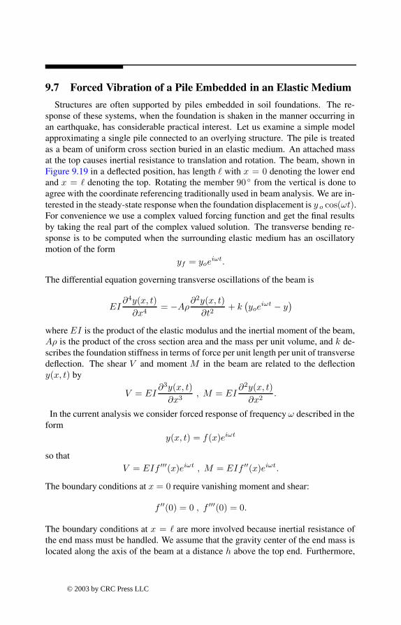
9.7 Forced Vibration of a Pile Embedded in an Elastic Medium

Structures are often supported by piles embedded in soil foundations. The re-sponse of these systems, when the foundation is shaken in the manner occurring inan earthquake, has considerable practical interest. Let us examine a simple modelapproximating a single pile connected to an overlying structure. The pile is treatedas a beam of uniform cross section buried in an elastic medium. An attached massat the top causes inertial resistance to translation and rotation. The beam, shown inFigure 9.19 in a deßected position, has length with x = 0 denoting the lower endand x = denoting the top. Rotating the member 90 from the vertical is done toagree with the coordinate referencing traditionally used in beam analysis. We are in-terested in the steady-state response when the foundation displacement is y o cos(ωt).For convenience we use a complex valued forcing function and get the Þnal resultsby taking the real part of the complex valued solution. The transverse bending re-sponse is to be computed when the surrounding elastic medium has an oscillatorymotion of the form

yf = yoeiωt.

The differential equation governing transverse oscillations of the beam is

EI∂4y(x, t)∂x4

= −Aρ∂2y(x, t)∂t2

+ k(yoe

iωt − y)

where EI is the product of the elastic modulus and the inertial moment of the beam,Aρ is the product of the cross section area and the mass per unit volume, and k de-scribes the foundation stiffness in terms of force per unit length per unit of transversedeßection. The shear V and moment M in the beam are related to the deßectiony(x, t) by

V = EI∂3y(x, t)∂x3

, M = EI∂2y(x, t)∂x2

.

In the current analysis we consider forced response of frequency ω described in theform

y(x, t) = f(x)eiωt

so thatV = EIf ′′′(x)eiωt , M = EIf ′′(x)eiωt.

The boundary conditions at x = 0 require vanishing moment and shear:

f ′′(0) = 0 , f ′′′(0) = 0.

The boundary conditions at x = are more involved because inertial resistance ofthe end mass must be handled. We assume that the gravity center of the end mass islocated along the axis of the beam at a distance h above the top end. Furthermore,


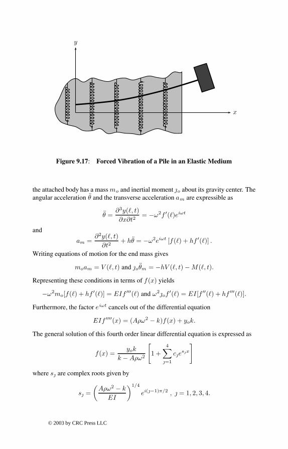
x

y

Figure 9.17: Forced Vibration of a Pile in an Elastic Medium

the attached body has a massmo and inertial moment o about its gravity center. Theangular acceleration θ and the transverse acceleration am are expressible as

θ =∂3y(, t)∂x∂t2

= −ω2f ′()eiωt

and

am =∂2y(, t)∂t2

+ hθ = −ω2eiωt [f() + hf ′()] .

Writing equations of motion for the end mass gives

moam = V (, t) and oθm = −hV (, t) −M(, t).

Representing these conditions in terms of f(x) yields

−ω2mo[f() + hf ′()] = EIf ′′′() and ω2of′() = EI[f ′′() + hf ′′′()].

Furthermore, the factor eiωt cancels out of the differential equation

EIf ′′′′(x) = (Aρω2 − k)f(x) + yok.

The general solution of this fourth order linear differential equation is expressed as

f(x) =yok

k −Aρω2

[1 +

4∑=1

cesx

]

where s are complex roots given by

s =(Aρω2 − k

EI

)1/4

ei(−1)π/2 , = 1, 2, 3, 4.


The conditions of zero moment and shear at x = 0 lead to

4∑=1

s2 c = 0 ,4∑

=0

s3 c = 0.

The shear and moment conditions at x = require

4∑=1

s3esc = −moω

2

[1 +

4∑=1

(1 + hs)esc

]

and4∑

=1

(s2 + hs3 )esc = oω

24∑

=1

sesc.

The system of four simultaneous equations can be solved for c 1, . . . , c4. Then theforced response solution corresponding to a foundation motion

real(yoe

ıωt)

= yo cos(ωt)

is given byy(x, t) = real

(f(x)eiωt

)where f(x) is complex valued.

The function pilevibs evaluates the displacement, moment, and shear for 0 ≤ x ≤, 0 ≤ t ≤ 2π/ω. Surface plots of these quantities are shown in Figures 9.18 through9.20. Figure 9.21 is a single frame from an animation depicting how the pile and theattached mass move.


0

50

100

150

0

2

4

6

8−0.8

−0.6

−0.4

−0.2

0

0.2

0.4

0.6

0.8

x axis

Deflection Surface for a Vibrating Pile

t*w axis

tran

sver

se d

efle

ctio

n

Figure 9.18: Deßection Surface for a Vibrating Pile

0

50

100

150

0

2

4

6

8−2

−1.5

−1

−0.5

0

0.5

1

1.5

2

x 105

x axis

Bending Moment in the Pile

t*w axis

bend

ing

mom

ent

Figure 9.19: Bending Moment in a Vibrating Pile


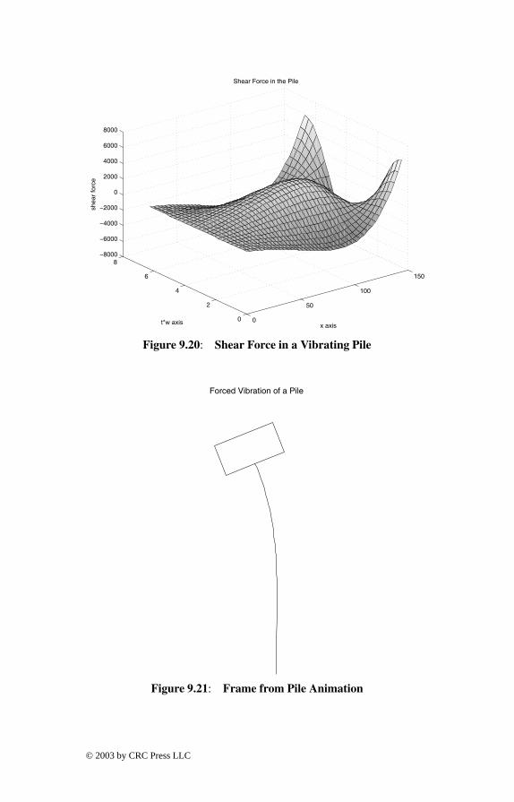
0

50

100

150

0

2

4

6

8−8000

−6000

−4000

−2000

0

2000

4000

6000

8000

x axis

Shear Force in the Pile

t*w axis

shea

r fo

rce

Figure 9.20: Shear Force in a Vibrating Pile

Forced Vibration of a Pile

Figure 9.21: Frame from Pile Animation


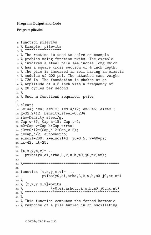
Program Output and Code

Program pilevibs

1: function pilevibs2: % Example: pilevibs3: % ~~~~~~~~~~~~~~~~~4: % The routine is used to solve an example5: % problem using function pvibs. The example6: % involves a steel pile 144 inches long which7: % has a square cross section of 4 inch depth.8: % The pile is immersed in soil having an elastic9: % modulus of 200 psi. The attached mass weighs

10: % 736 lb. The foundation is shaken at an11: % amplitude of 0.5 inch with a frequency of12: % 20 cycles per second.13: %14: % User m functions required: pvibs15:

16: clear;17: L=144; d=4; a=d^2; I=d^4/12; e=30e6; ei=e*I;18: g=32.2*12; Density_steel=0.284;19: rho=Density_steel/g;20: Cap_w=36; Cap_h=18; Cap_t=4;21: m0=Cap_w*Cap_h*Cap_t*rho;22: j0=m0/12*(Cap_h^2+Cap_w^2);23: h=Cap_h/2; arho=a*rho;24: e_soil=200; k=e_soil*d; y0=0.5; w=40*pi;25: nx=42; nt=25;26:

27: [t,x,y,m,v]= ...28: pvibs(y0,ei,arho,L,k,w,h,m0,j0,nx,nt);29:

30: %=============================================31:

32: function [t,x,y,m,v]= ...33: pvibs(y0,ei,arho,L,k,w,h,m0,j0,nx,nt)34: %35: % [t,x,y,m,v]=pvibs ...36: % (y0,ei,arho,L,k,w,h,m0,j0,nx,nt)37: % ~~~~~~~~~~~~~~~~~~~~~~~~~~~~~~~~~~~~~~~~~~~~38: %39: % This function computes the forced harmonic40: % response of a pile buried in an oscillating


41: % elastic medium. The lower end of the pile is42: % free from shear and moment. The top of the43: % pile carries an attached body having general44: % mass and inertial properties. The elastic45: % foundation is given a horizontal oscillation46: % of the form47: %48: % yf=real(y0*exp(i*w*t))49: %50: % The resulting transverse forced response of51: % the pile is expressed as52: %53: % y(x,t)=real(f(x)*exp(i*w*t))54: %55: % where f(x) is a complex valued function. The56: % bending moment and shear force in the pile57: % are also computed.58: %59: % y0 - amplitude of the foundation oscillation60: % ei - product of moment of inertia and61: % elastic modulus for the pile62: % arho - mass per unit length of the pile63: % L - pile length64: % k - the elastic resistance constant for the65: % foundation described as force per unit66: % length per unit of transverse67: % deflection68: % w - the circular frequency of the69: % foundation oscillation which vibrates70: % like real(y0*exp(i*w*t))71: % h - the vertical distance above the pile72: % upper end to the gravity center of the73: % attached body74: % m0 - the mass of the attached body75: % j0 - the mass moment of inertia of the76: % attached body with respect to its77: % gravity center78: % nx - the number of equidistant values along79: % the pile at which the solution is80: % computed81: % nt - the number of values of t values at82: % which the solution is computed such83: % that 0 <= w*t <= 2*pi84: %85: % t - a vector of time values such that the


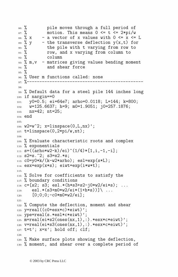
86: % pile moves through a full period of87: % motion. This means 0 <= t <= 2*pi/w88: % x - a vector of x values with 0 <= x <= L89: % y - the transverse deflection y(x,t) for90: % the pile with t varying from row to91: % row, and x varying from column to92: % column93: % m,v - matrices giving values bending moment94: % and shear force95: %96: % User m functions called: none97: %----------------------------------------------98:

99: % Default data for a steel pile 144 inches long100: if nargin==0101: y0=0.5; ei=64e7; arho=0.0118; L=144; k=800;102: w=125.6637; h=9; m0=1.9051; j0=257.1876;103: nx=42; nt=25;104: end105:

106: w2=w^2; x=linspace(0,L,nx)’;107: t=linspace(0,2*pi/w,nt);108:

109: % Evaluate characteristic roots and complex110: % exponentials111: s=((arho*w2-k)/ei)^(1/4)*[1,i,-1,-i];112: s2=s.^2; s3=s2.*s;113: c0=y0*k/(k-w2*arho); esl=exp(s*L);114: esx=exp(x*s); eiwt=exp(i*w*t);115:

116: % Solve for coefficients to satisfy the117: % boundary conditions118: c=[s2; s3; esl.*(h*s3+s2-j0*w2/ei*s); ...119: esl.*(s3+m0*w2/ei*(1+h*s))]\ ...120: [0;0;0;-c0*m0*w2/ei];121:

122: % Compute the deflection, moment and shear123: y=real((c0+esx*c)*eiwt)’;124: ype=real(s.*esl*c*eiwt)’;125: m=real(ei*s2(ones(nx,1),:).*esx*c*eiwt)’;126: v=real(ei*s3(ones(nx,1),:).*esx*c*eiwt)’;127: t=t’; x=x’; hold off; clf;128:

129: % Make surface plots showing the deflection,130: % moment, and shear over a complete period of


131: % the motion132: surf(x,t*w,y);133: xlabel(’x axis’); ylabel(’t*w axis’);134: zlabel(’transverse deflection’);135: title(’Deflection Surface for a Vibrating Pile’);136: grid on; figure(gcf)137: % print -deps pilesurf138: disp(’Press [Enter] to continue’), pause139:

140: surf(x,t*w,m);141: xlabel(’x axis’); ylabel(’t*w axis’);142: zlabel(’bending moment’);143: title(’Bending Moment in the Pile’)144: grid on; figure(gcf)145: % print -deps pilemom;146: disp(’Press [Enter] to continue’), pause147:

148: surf(x,t*w,v);149: xlabel(’x axis’); ylabel(’t*w axis’);150: zlabel(’shear force’);151: title(’Shear Force in the Pile’);152: grid on; figure(gcf)153: % print -deps pilesher154: disp(’Press [Enter] to see animation’), pause155:

156: % Draw an animation depicting the pile response157: % to the oscillation of the foundation158: fu=.10/max(y(:)); p=[-0.70, 0.70, -.1, 1.3];159: u=fu*y; upe=fu*L*ype; d=.15;160: xm=[0,0,1,1,0,0]*d;161: ym=[0,-1,-1,1,1,0]*d; zm=xm+i*ym;162: close;163: for jj=1:4164: for j=1:nt165: z=exp(i*atan(upe(j)))*zm;166: xx=real(z); yy=imag(z);167: ut=[u(j,:),u(j,nx)+yy]; xt=[x/L,1+xx];168: plot(ut,xt,’-’); axis(p); axis(’square’);169: title(’Forced Vibration of a Pile’);170: axis(’off’); drawnow; figure(gcf);171: end172: end173: % print -deps pileanim174: fprintf(’\nAll Done\n’);


9.8 Transient Heat Conduction in a One-Dimensional Slab

Let us analyze the temperature history in a slab which has the left side insulatedwhile the right side temperature varies sinusoidally according to U 0 sin(ΩT ). Theinitial temperature in the slab is speciÞed to be zero. The pertinent boundary valueproblem is

α∂2U

∂X2(X,T ) =

∂U

∂T(X,T ) , 0 < X < , T > 0,

∂U

∂X(0, T ) = 0 , U(, T ) = U0 sin(ΩT ),

U(X, 0) = 0 , 0 < X <

where U , X , T , and α are, respectively, the temperature, position, time, and thermaldiffusivity.

The problem can be converted to dimensionless form by letting

u =U

U0, x =

X

, t =

αT

2, ω =

Ω2

α.

Then we get∂2u

∂x2=∂u

∂x, 0 < x < 1 , t > 0,

∂u

∂x(0, t) = 0 , u(1, t) = imag

(eiωt

), u(x, 0) = 0.

The solution consists of two parts as u = w + v, where w is a particular solutionsatisfying the differential equation and nonhomogeneous boundary conditions, andv is a solution satisfying homogeneous boundary conditions and speciÞed to imposethe desired zero initial temperature when combined with w. The appropriate formfor the particular solution is

w = imag[f(x)eiωt

].

Making w satisfy the heat equation requires

f ′′(x) = iwf(x).

Consequentlyf(x) = c1 sin(φx) + c2 cos(φx)

where φ =√−ıω. The conditions of zero gradient at x = 0 and unit function value

at x = 1 determine c1 and c2. We get the particular solution as

w = imag[cos(φx)cos(φ)

eiωt

].


This forced response solution evaluated at t = 0 yields

w(x, 0) = imag[cos(φx)cos(φ)

].

The general solution of the heat equation satisfying zero gradient at x = 0 and zerofunction value at x = 1 is found to be

v(x, t) =∞∑

n=1

an cos(λnx)e−λ2nt

where λn = π(2n−1)/2. To make the initial temperature equal zero in the combinedsolution, the coefÞcients an are chosen to satisfy

∞∑n=1

an cos(λnx) = − imag[cos(φx)cos(φ)

].

The orthogonality of the functions cos(λnx) implies

an = −2∫ 1

0

imag[cos(φx)cos(φ)

]cos(λnx)dx

which can be integrated to give

an = − imag[(sin(λn + φ)/(λn + φ) + sin(λn − φ)/(λn − φ))

cos(φ)

].

This completely determines the solution. Taking any Þnite number of terms in theseries produces an approximate solution exactly satisfying the differential equationand boundary conditions. Exact satisfaction of the zero initial condition would theo-retically require an inÞnite number of series terms. However, the terms in the seriesdecrease like O(1/n3) and using a 250-term series produces initial temperature val-ues not exceeding 10−6. Thus, the Þnite series is satisfactory for practical purposes.

The above equations were evaluated in a function called heat. Function slab-heat was also written to plot numerical results. The code and resulting Figures 9.23and 9.24 appear below. This example illustrates nicely how well MATLAB handlescomplex arithmetic and complex valued functions.


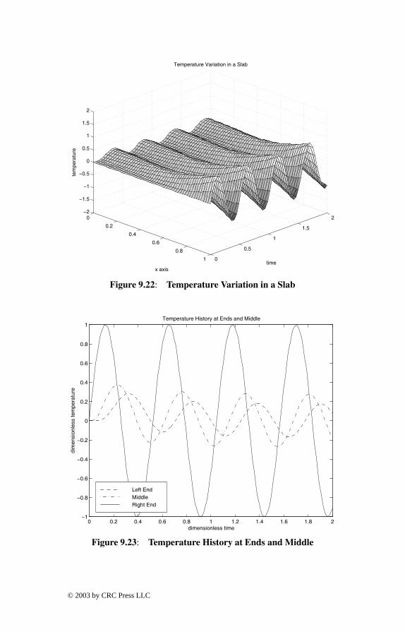
0

0.2

0.4

0.6

0.8

1 0

0.5

1

1.5

2−2

−1.5

−1

−0.5

0

0.5

1

1.5

2

time

Temperature Variation in a Slab

x axis

tem

pera

ture

Figure 9.22: Temperature Variation in a Slab

0 0.2 0.4 0.6 0.8 1 1.2 1.4 1.6 1.8 2−1

−0.8

−0.6

−0.4

−0.2

0

0.2

0.4

0.6

0.8

1Temperature History at Ends and Middle

dimensionless time

dim

ensi

onle

ss te

mpe

ratu

re

Left End Middle Right End

Figure 9.23: Temperature History at Ends and Middle


Heat Conduction Program

Program slabheat

1: function slabheat2: % Example: slabheat3: % ~~~~~~~~~~~~~~~~~4: % This program computes the temperature5: % variation in a one-dimensional slab with6: % the left end insulated and the right end7: % given a temperature variation sin(w*t).8: %9: % User m functions required: heat

10:

11: [u1,t1,x1]=heat(12,0,2,50,0,1,51,250);12: surf(x1,t1,u1); axis([0 1 0 2 -2 2]);13: title(’Temperature Variation in a Slab’);14: xlabel(’x axis’); ylabel(’time’);15: zlabel(’temperature’); view([45,30])16: colormap(’default’), shg17: disp(’ ’), disp(’Press [Enter] to continue’)18: pause19: % print -deps tempsurf20:

21: [u2,t2,x2]=heat(12,0,2,150,0,1,3,250);22: plot(t2,u2(:,1),’--’,t2,u2(:,2),’:’, ...23: t2,u2(:,3),’-’);24: title([’Temperature History at Ends’ ...25: ’ and Middle’]);26: xlabel(’dimensionless time’);27: ylabel(’dimensionless temperature’);28: text1=’Left End’; text2=’Middle’;29: text3=’Right End’;30: legend(text1,text2,text3,3); shg31: % print -deps templot32: disp(’ ’), disp(’All Done’);33:

34: %=============================================35:

36: function [u,t,x]= ...37: heat(w,tmin,tmax,nt,xmin,xmax,nx,nsum)38: %39: %[u,t,x]=heat(w,tmin,tmax,nt,xmin,xmax,nx,nsum)40: %~~~~~~~~~~~~~~~~~~~~~~~~~~~~~~~~~~~~~~~~~~~~~~


41: % This function evaluates transient heat42: % conduction in a slab which has the left end43: % (x=0) insulated and has the right end (x=1)44: % subjected to a temperature variation45: % sin(w*t). The initial temperature of the slab46: % is zero.47: %48: % w - frequency of the right side49: % temperature variation50: % tmin,tmax - time limits for solution51: % nt - number of uniformly spaced52: % time values used53: % xmin,xmax - position limits for solution.54: % Values should lie between zero55: % and one.56: % nx - number of equidistant x values57: % nsum - number of terms used in the58: % series solution59: % u - matrix of temperature values.60: % Time varies from row to row.61: % x varies from column to column.62: % t,x - vectors of time and x values63: %64: % User m functions called: none.65: %----------------------------------------------66:

67: t=tmin+(tmax-tmin)/(nt-1)*(0:nt-1);68: x=xmin+(xmax-xmin)/(nx-1)*(0:nx-1)’;69: W=sqrt(-i*w); ln=pi*((1:nsum)-1/2);70: v1=ln+W; v2=ln-W;71: a=-imag((sin(v1)./v1+sin(v2)./v2)/cos(W));72: u=imag(cos(W*x)*exp(i*w*t)/cos(W))+ ...73: (a(ones(nx,1),:).*cos(x*ln))* ...74: exp(-ln(:).^2*t);75: u=u’; t=t(:);

9.9 Transient Heat Conduction in a Circular Cylinder with Spa-tially Varying Boundary Temperature

9.9.1 Problem Formulation

Transient heat conduction in a circular cylinder can be analyzed using an inÞniteseries of Bessel functions. Consider a cylinder having an initial temperature distri-


bution u0(r, θ) when the boundary is suddenly given a temperature variation f(θ)depending on the polar angle but independent of time. The problem is convenientlyformulated in polar coordinates using dimensionless radius and time variables. Thedifferential equation, boundary conditions, and initial conditions are as follows:

urr +1rur +

1r2uθθ = ut , 0 ≤ r ≤ 1 , t > 0,

u(1, θ, t) = f(θ) =∞∑

n=−∞fne

inϑ , 0 ≤ θ ≤ 2π,

u(r, θ, 0) = u0(r, θ) , 0 ≤ r ≤ 1 , 0 ≤ θ ≤ 2π.

With the boundary condition expressed as a complex Fourier series, the steady-statesolution satisfying the differential equation and the boundary conditions is

v(r, θ) = −f0 + 2 real

( ∞∑n=0

fnzn

)where z = reiθ .

The total solution is the steady-state solution combined with a transient solutionw(r, θ, t) chosen to satisfy the initial condition and boundary conditions expressedas

w(r, θ, 0) = u0(r, θ) − v(r, θ) , w(1, θ, t) = 0.

The transient solution is a Fourier-Bessel series involving double subscripted coefÞ-cients depending on the functions v(r, θ) and u0(r, θ). It is found that

w(r, θ, t) =∞∑

n=0

∞∑k=1

Jn(λnkr) [Ank cos(nθ) +Bnk sin(nθ)] exp(−λ2nkt)

where, for n > 0 and k ≥ 1, we have

Ank + iBnk = Cnk =2

πJ2n+1(λnk)

2π∫0

1∫0

w(r, θ, 0)rJn(λnkr) exp(inθ)drdθ

with λnk denoting the k ′th positive root of Jn(r). The last formula almost applies forn = 0 except that A0k = C0k/2 and B0k = 0. The coefÞcients for n = 0 pertainto the radially symmetric case independent of the polar angle. Evaluating this seriessolution involves several steps which are: 1) Expanding the boundary condition in acomplex Fourier series to obtain the steady-state solution; 2) Determining the zerosof the integer order Bessel functions Jn(r); 3) Computing the series coefÞcients bynumerical integration; and 4) Summing the series solution for various (r, θ) valueswith enough terms being used in the series to assure adequate satisfaction of theinitial conditions and boundary conditions.


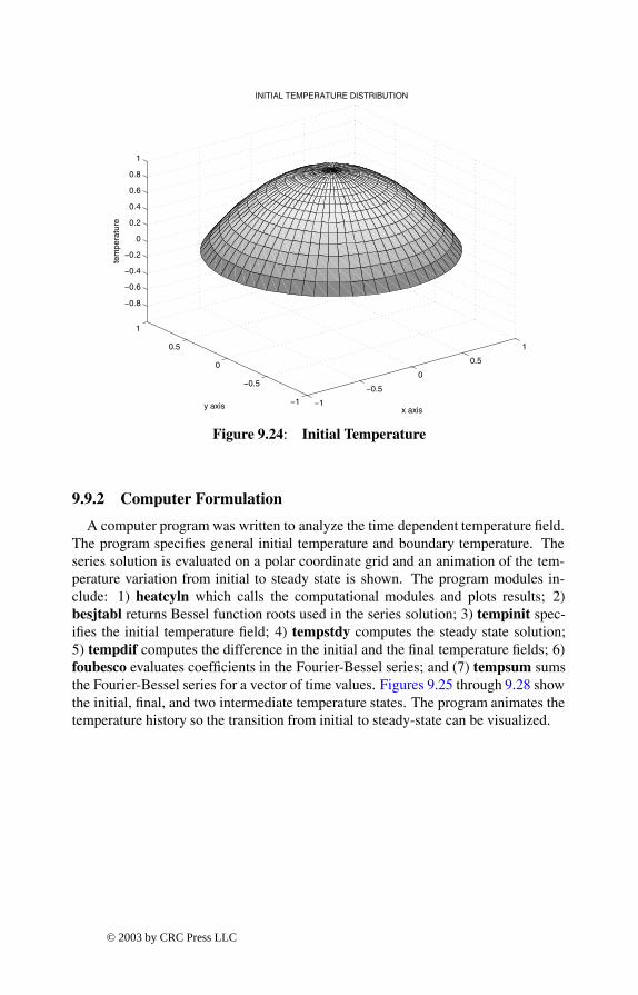
−1

−0.5

0

0.5

1

−1

−0.5

0

0.5

1

−0.8

−0.6

−0.4

−0.2

0

0.2

0.4

0.6

0.8

1

x axis

INITIAL TEMPERATURE DISTRIBUTION

y axis

tem

pera

ture

Figure 9.24: Initial Temperature

9.9.2 Computer Formulation

A computer program was written to analyze the time dependent temperature Þeld.The program speciÞes general initial temperature and boundary temperature. Theseries solution is evaluated on a polar coordinate grid and an animation of the tem-perature variation from initial to steady state is shown. The program modules in-clude: 1) heatcyln which calls the computational modules and plots results; 2)besjtabl returns Bessel function roots used in the series solution; 3) tempinit spec-iÞes the initial temperature Þeld; 4) tempstdy computes the steady state solution;5) tempdif computes the difference in the initial and the Þnal temperature Þelds; 6)foubesco evaluates coefÞcients in the Fourier-Bessel series; and (7) tempsum sumsthe Fourier-Bessel series for a vector of time values. Figures 9.25 through 9.28 showthe initial, Þnal, and two intermediate temperature states. The program animates thetemperature history so the transition from initial to steady-state can be visualized.


−1

−0.5

0

0.5

1

−1

−0.5

0

0.5

1

−0.8

−0.6

−0.4

−0.2

0

0.2

0.4

0.6

0.8

1

x axis

Temperature at time = 0.020

y axis

tem

pera

ture

Figure 9.25: Temperature at t=0.02

−1

−0.5

0

0.5

1

−1

−0.5

0

0.5

1

−0.8

−0.6

−0.4

−0.2

0

0.2

0.4

0.6

0.8

1

x axis

Temperature at time = 0.050

y axis

tem

pera

ture

Figure 9.26: Temperature at t=0.05


−1

−0.5

0

0.5

1

−1

−0.5

0

0.5

1

−0.8

−0.6

−0.4

−0.2

0

0.2

0.4

0.6

0.8

1

x axis

STEADY STATE TEMPERATURE DISTRIBUTION

y axis

tem

pera

ture

Figure 9.27: Steady State Temperature


Program heatcyln

1: function heatcyln2: %3: % heatcyln4: % ~~~~~~~~5: % This program analyzes the time varying temperature6: % history in a circular cylinder which initially has7: % a radially symmetric temperature varying para-8: % bolically. Then a spatially varying but constant9: % boundary temperature distribution is imposed. The

10: % total solution is composed of a harmonic steady11: % state solution plus a transient component given by12: % a Fourier-Bessel series.13: % User functions called:14: % besjtabl, tempinit, tempstdy, foubesco,15: % tempsum, tempdif, gcquad16:

17: global ubdry besjrt18:

19: % Obtain Bessel function roots needed in the20: % transient solution21: besjrt=besjtabl(0:20,20);22:

23: % Define the steady state temperature imposed24: % on the outer boundary for t>025: th=linspace(0,pi,100)’;26: ud=cos(2*th).*(th<=pi/2)+...27: (-3+4/pi*th).*(th>pi/2&th<3*pi/4);28: ud=[ud;ud(end-1:-1:1)];29: ubdry=[linspace(0,360,199)’,ud];30: theta=linspace(0,2*pi,65);31: r=linspace(0,1,15);32:

33: % Compute and plot the initial and final34: % temperature fields35: [uinit,z]=tempinit(theta,r);36: [usteady,z]=tempstdy(theta,r);37: umin=min([usteady(:);uinit(:)]);38: umax=max([usteady(:);uinit(:)]);39: range=[-1,1,-1,1,umin,umax];40: x=real(z); y=imag(z);41:


42: surf(x,y,uinit), colormap(’default’)43: title(’INITIAL TEMPERATURE DISTRIBUTION’)44: xlabel(’x axis’), ylabel(’y axis’)45: zlabel(’temperature’), axis(range), disp(’ ’)46: disp(’Press [Enter] to see the steady’)47: disp(’state temperature distribution’)48: shg, pause, disp(’ ’)49: % print -deps tempinit50:

51: surf(x,y,usteady)52: title(’STEADY STATE TEMPERATURE DISTRIBUTION’)53: xlabel(’x axis’), ylabel(’y axis’)54: zlabel(’temperature’), axis(range), shg55: % print -deps tempstdy56:

57: % Compute coefficients used in the Fourier-58: % Bessel series for the transient solution59: [c,lam,cptim]=foubesco(@tempdif,20,20,40,128);60:

61: % Set a time interval sufficient to nearly62: % reach steady state63: tmax=.4; nt=81; t=linspace(0,tmax,nt);64:

65: % Evaluate the transient solution66: [u,tsum]=tempsum(c,theta,r,t,lam);67: u(:,:,1)=uinit-usteady;68:

69: % Plot time history for the total solution70: while 171: disp(’Press [Enter] to see the animation’)72: disp(’or enter 0 to stop’), v=input(’> ? ’);73: if isempty(v), v=1; end74: if v~=1, break, end75: for j=1:nt76: utotal=usteady+u(:,:,j);77: surf(x,y,utotal)78: titl=sprintf([’Temperature at time =’,...79: ’%6.3f’],t(j)); title(titl)80: xlabel(’x axis’), ylabel(’y axis’)81: zlabel(’temperature’), axis(range);82: drawnow; shg, pause(.3)83: end84: end85:

86: %=============================================


87:

88: function [u,z]=tempstdy(theta,r)89: %90: % [u,z]=tempstdy(theta,r)91: % ~~~~~~~~~~~~~~~~~~~~~~92: % Steady state temperature distribution in a93: % circular cylinder of unit radius with94: % piecewise linear boundary values95: % described in global array ubdry.96: global ubdry97:

98: thft=2*pi/(1024)*(0:1023); n=100;99: ufft=interp1(pi/180*ubdry(:,1),...

100: ubdry(:,2)/1024,thft);101: c=fft(ufft); z=exp(i*theta(:))*r(:)’;102: u=-real(c(1))+2*real(...103: polyval(c(n:-1:1),z));104:

105: %=============================================106:

107: function [u,z]=tempinit(theta,r)108: %109: % [u,z]=tempinit(theta,r)110: % ~~~~~~~~~~~~~~~~~~~~~~111: % Initial temperature varying parabolically112: % with the radius113: theta=theta(:); r=r(:)’; z=exp(i*theta)*r;114: u=ones(length(theta),1)*(1-r.^2);115:

116: %=============================================117:

118: function [u,z]=tempdif(theta,r)119: %120: % [u,z]=tempdif(theta,r)121: % ~~~~~~~~~~~~~~~~~~~~~122: % Difference between the steady state temp-123: % erature and the initial temperature124: u1=tempstdy(theta,r); [u2,z]=tempinit(theta,r);125: u=u2-u1;126:

127: %=============================================128:

129: function [c,lam,cptim]=foubesco(...130: f,nord,nrts,nrquad,nft)131: %


132: % [c,lam,cptim]=foubesco(f,nord,nrts,nrquad,nft)133: % ~~~~~~~~~~~~~~~~~~~~~~~~~~~~~~~~~~~~~~~~~~~~~134: % Fourier-Bessel coefficients computed using the135: % FFT136: global besjrt137: if nargin<5, nft=128; end138: if nargin<4, nrquad=50; end139: if nargin<3, nrts=10; end140: if nargin<2, nord=10; end141: if nargin==0, f=’fbes’; end142: tic; lam=besjrt(1:nord,1:nrts);143: c=zeros(nord,nrts);144: [dummy,r,w]=gcquad([],0,1,nrquad,1);145: r=r(:)’; w=w(:)’; th=2*pi/nft*(0:nft-1)’;146: fmat=fft(feval(f,th,r));147: fmat=fmat(1:nord,:).*repmat(r.*w,nord,1);148: for n=1:nord149: for k=1:nrts150: lnk=lam(n,k);151: v=sum(fmat(n,:).*besselj(n-1,lnk*r));152: c(n,k)=4*v/nft/besselj(n,lnk).^2;153: end154: end155: c(1,:)=c(1,:)/2; cptim=toc;156:

157: %=============================================158:

159: function [u,tcpu]=tempsum(c,th,r,t,lam)160: %161: % [u,tsum]=tempsum(c,th,r,t,lam)162: %163: % This function sums a Fourier-Bessel series164: % for transient temperature history in a circular165: % cylinder with given initial conditions and166: % zero temperature at the boundary. The series167: % has the form168: % u(theta,r,t)=sum(n=0:nord-1),k=1:nrts,...169: % besselj(n,lam(n+1,k)*r)*real(...170: % c(n+1,k)*exp(i*(n+1)*theta))*...171: % exp(-lam(n+1,k)^2*t), where172: % besselj(n-1,lam(n,k))=0 and173: % [nord,nrts]=size(c)174: %175: % c - the series coefficients for the initial176: % temperature distribution obtained using


177: % function foubesco178: % th - vector or theta values between179: % zero and 2*pi180: % r - vector of radius values between181: % zero and one182: % lam - matrix of bessel function roots.183: % If this argument is omitted, then184: % function besjroot is called to185: % compute the roots186: % u - a three-dimensional array of function187: % values where u(i,j,k) contains the188: % temperature for theta(i), r(j), t(k)189: % tcpu - computation time in seconds190:

191: tic; [nord,nrts]=size(c);192: if nargin<5, lam=besjroot(0:nord-1,nrts); end193: th=th(:); nth=length(th); r=r(:)’; nr=length(r);194: nt=length(t); N=repmat((0:nord-1)’,1,nrts);195: N=N(:)’; c=c(:).’; lam=lam(:); lam2=-(lam.^2)’;196: u=zeros(nth,nr,nt); thmat=exp(i*th*N);197: besmat=besselj(repmat(N’,1,nr),lam*r);198: for I=1:nt199: C=c.*exp(lam2*t(I));200: u(:,:,I)=real(thmat.*repmat(C,nth,1))*besmat;201: end202: tcpu=toc;203:

204: %=============================================205:

206: function r=besjtabl(nordr,nrts)207: %208: % r=besjtable(nordr,nrts)209: % ~~~~~~~~~~~~~~~~~~~~~210: % This function returns a table for roots of211: % besselj(n,x)=0 accurate to about five digits.212: % r(k,:) - contains the first 20 positive roots of213: % besselj(k-1,x)=0; for k=1:21214: % nordr - a vector of function orders lying215: % between 0 and 20216: % nrts - the highest root order not to exceed217: % the twentieth positive root218:

219: if nargin==0, nordr=0:20; nrts=20; end220: if max(nordr)>20 | nrts>20, r=nan; return; end221: r=[2.4048 21.6415 40.7729 33.7758 53.7383 73.2731


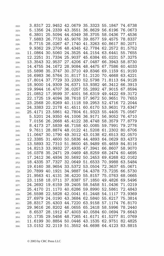
222: 3.8317 22.9452 42.0679 35.3323 55.1847 74.6738223: 5.1356 24.2339 43.3551 36.8629 56.6196 76.0673224: 6.3801 25.5094 44.6349 38.3705 58.0436 77.4536225: 7.5883 26.7733 45.9076 39.8577 59.4575 78.8337226: 8.7715 28.0267 47.1740 41.3263 60.8617 80.2071227: 9.9362 29.2706 48.4345 42.7784 62.2572 81.5752228: 11.0864 30.5060 24.3525 44.2154 63.6441 55.7655229: 12.2251 31.7334 25.9037 45.6384 65.0231 57.3275230: 13.3543 32.9537 27.4206 47.0487 66.3943 58.8730231: 14.4755 34.1672 28.9084 48.4475 67.7586 60.4033232: 15.5898 35.3747 30.3710 49.8346 69.1159 61.9193233: 16.6983 36.5764 31.8117 51.2120 70.4668 63.4221234: 17.8014 37.7729 33.2330 52.5798 71.8113 64.9128235: 18.9000 14.9309 34.6371 53.9382 46.3412 66.3913236: 19.9944 16.4707 36.0257 55.2892 47.9015 67.8594237: 21.0852 17.9599 37.4001 56.6319 49.4422 69.3172238: 22.1725 19.4094 38.7618 57.9672 50.9651 70.7653239: 23.2568 20.8269 40.1118 59.2953 52.4716 72.2044240: 24.3383 22.2178 41.4511 60.6170 53.9631 73.6347241: 25.4171 23.5861 42.7804 61.9323 55.4405 75.0567242: 5.5201 24.9350 44.1006 36.9171 56.9052 76.4710243: 7.0156 26.2668 45.4122 38.4748 58.3579 77.8779244: 8.4173 27.5839 46.7158 40.0085 59.7991 79.2776245: 9.7611 28.8874 48.0122 41.5208 61.2302 80.6706246: 11.0647 30.1790 49.3012 43.0138 62.6513 82.0570247: 12.3385 31.4600 50.5836 44.4893 64.0629 83.4373248: 13.5893 32.7310 51.8600 45.9489 65.4659 84.8116249: 14.8213 33.9932 27.4935 47.3941 66.8607 58.9070250: 16.0378 35.2471 29.0469 48.8259 68.2474 60.4695251: 17.2412 36.4934 30.5692 50.2453 69.6268 62.0162252: 18.4335 37.7327 32.0649 51.6533 70.9988 63.5484253: 19.6160 38.9654 33.5372 53.0504 72.3637 65.0671254: 20.7899 40.1921 34.9887 54.4378 73.7235 66.5730255: 21.9563 41.4131 36.4220 55.8157 75.0763 68.0665256: 23.1158 18.0711 37.8387 57.1850 49.4826 69.5496257: 24.2692 19.6159 39.2405 58.5458 51.0436 71.0219258: 25.4170 21.1170 40.6286 59.8990 52.5861 72.4843259: 26.5598 22.5828 42.0041 61.2448 54.1117 73.9369260: 27.6979 24.0190 43.3684 62.5840 55.6217 75.3814261: 28.8317 25.4303 44.7220 63.9158 57.1174 76.8170262: 29.9616 26.8202 46.0655 65.2418 58.5996 78.2440263: 8.6537 28.1912 47.4003 40.0584 60.0694 79.6643264: 10.1735 29.5456 48.7265 41.6171 61.5277 81.0769265: 11.6199 30.8854 50.0446 43.1535 62.9751 82.4825266: 13.0152 32.2119 51.3552 44.6698 64.4123 83.8815


267: 14.3726 33.5265 52.6589 46.1679 65.8399 85.2738268: 15.7002 34.8300 53.9559 47.6493 67.2577 86.6603269: 17.0037 36.1237 55.2466 49.1157 68.6681 88.0408270: 18.2876 37.4081 30.6346 50.5681 70.0699 62.0485271: 19.5546 38.6843 32.1897 52.0077 71.4639 63.6114272: 20.8070 39.9526 33.7166 53.4352 72.8506 65.1593273: 22.0470 41.2135 35.2187 54.8517 74.2302 66.6933274: 23.2758 42.4678 36.6990 56.2576 75.6032 68.2142275: 24.4949 43.7155 38.1598 57.6538 76.9699 69.7230276: 25.7051 44.9577 39.6032 59.0409 78.3305 71.2205277: 26.9074 21.2117 41.0308 60.4194 52.6241 72.7065278: 28.1024 22.7601 42.4439 61.7893 54.1856 74.1827279: 29.2909 24.2702 43.8439 63.1524 55.7297 75.6493280: 30.4733 25.7482 45.2315 64.5084 57.2577 77.1067281: 31.6501 27.1990 46.6081 65.8564 58.7709 78.5555282: 32.8218 28.6266 47.9743 67.1982 60.2703 79.9960283: 33.9887 30.0337 49.3308 68.5339 61.7567 81.4291284: 11.7916 31.4228 50.6782 43.1998 63.2313 82.8535285: 13.3237 32.7958 52.0172 44.7593 64.6947 84.2714286: 14.7960 34.1543 53.3483 46.2980 66.1476 85.6825287: 16.2234 35.4999 54.6719 47.8178 67.5905 87.0870288: 17.6159 36.8336 55.9885 49.3204 69.0240 88.4846289: 18.9801 38.1563 57.2984 50.8072 70.4486 89.8772290: 20.3208 39.4692 58.6020 52.2794 71.8648 91.2635];291: r=reshape(r(:),21,20); r=r(1+nordr,1:nrts);292:

293: %=============================================294:

295: % function [val,bp,wf]=gcquad(func,xlow,...296: % xhigh,nquad,mparts,varargin)297: % See Appendix B

9.10 Torsional Stresses in a Beam of Rectangular Cross Section

Elastic beams of uniform cross section are commonly used structural members.Evaluation of the stresses caused when beams undergo torsional moments dependson Þnding a particular type of complex valued function. This function is analyticinside the beam cross section and has its imaginary part known on the boundary[72]. The shear stresses τXZ and τY Z are obtained from the stress function f(z) ofthe complex variable z = x+ iy according to

τZX − iτZY

µα= f ′(z) − iz


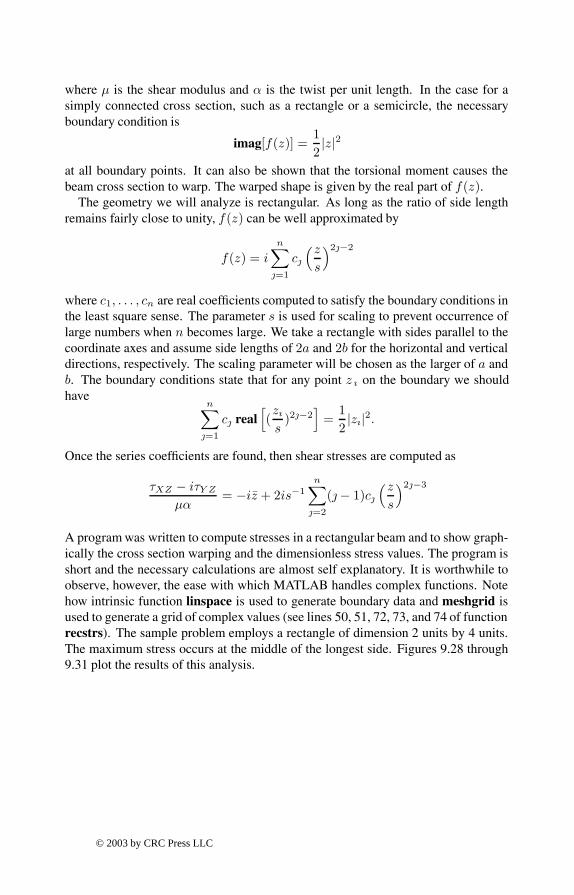
where µ is the shear modulus and α is the twist per unit length. In the case for asimply connected cross section, such as a rectangle or a semicircle, the necessaryboundary condition is

imag[f(z)] =12|z|2

at all boundary points. It can also be shown that the torsional moment causes thebeam cross section to warp. The warped shape is given by the real part of f(z).

The geometry we will analyze is rectangular. As long as the ratio of side lengthremains fairly close to unity, f(z) can be well approximated by

f(z) = in∑

=1

c

(zs

)2−2

where c1, . . . , cn are real coefÞcients computed to satisfy the boundary conditions inthe least square sense. The parameter s is used for scaling to prevent occurrence oflarge numbers when n becomes large. We take a rectangle with sides parallel to thecoordinate axes and assume side lengths of 2a and 2b for the horizontal and verticaldirections, respectively. The scaling parameter will be chosen as the larger of a andb. The boundary conditions state that for any point z ı on the boundary we shouldhave

n∑=1

c real[(zı

s)2−2

]=

12|zı|2.

Once the series coefÞcients are found, then shear stresses are computed as

τXZ − iτY Z

µα= −iz + 2is−1

n∑=2

(− 1)c(zs

)2−3

A program was written to compute stresses in a rectangular beam and to show graph-ically the cross section warping and the dimensionless stress values. The program isshort and the necessary calculations are almost self explanatory. It is worthwhile toobserve, however, the ease with which MATLAB handles complex functions. Notehow intrinsic function linspace is used to generate boundary data and meshgrid isused to generate a grid of complex values (see lines 50, 51, 72, 73, and 74 of functionrecstrs). The sample problem employs a rectangle of dimension 2 units by 4 units.The maximum stress occurs at the middle of the longest side. Figures 9.28 through9.31 plot the results of this analysis.


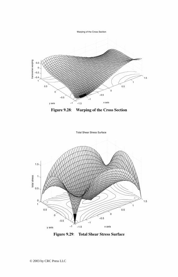
−1.5

−1

−0.5

0

0.5

1

1.5

−1

−0.5

0

0.5

1

−0.4

−0.2

0

0.2

x axis

Warping of the Cross Section

y axis

tran

sver

se w

arpi

ng

Figure 9.28: Warping of the Cross Section

−1.5

−1

−0.5

0

0.5

1

1.5

−1

−0.5

0

0.5

1

0

0.5

1

1.5

x axis

Total Shear Stress Surface

y axis

tota

l str

ess

Figure 9.29: Total Shear Stress Surface


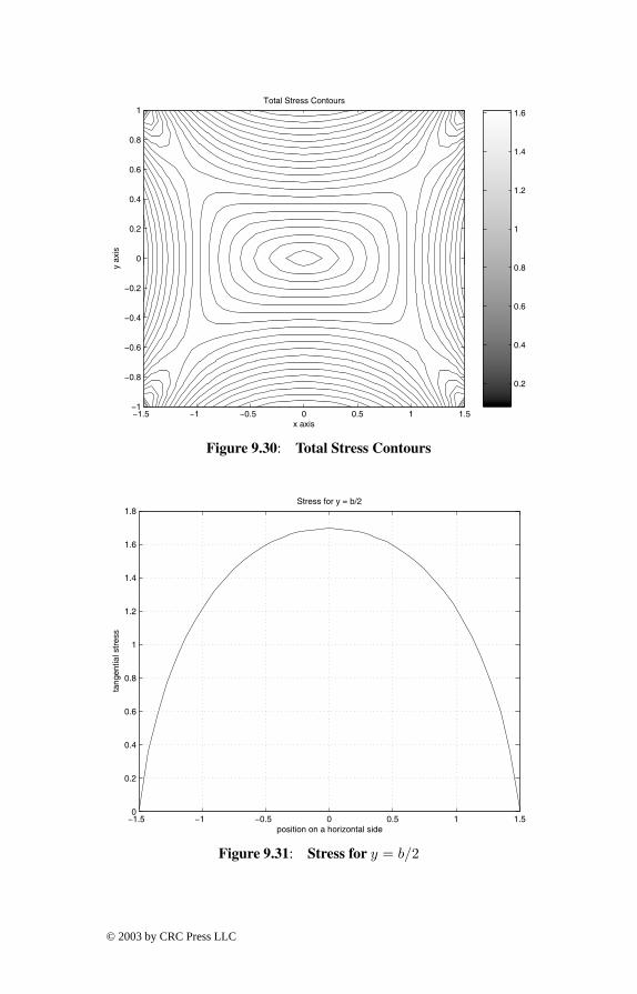
−1.5 −1 −0.5 0 0.5 1 1.5−1

−0.8

−0.6

−0.4

−0.2

0

0.2

0.4

0.6

0.8

1

x axis

y ax

is

Total Stress Contours

0.2

0.4

0.6

0.8

1

1.2

1.4

1.6

Figure 9.30: Total Stress Contours

−1.5 −1 −0.5 0 0.5 1 1.50

0.2

0.4

0.6

0.8

1

1.2

1.4

1.6

1.8

tang

entia

l str

ess

position on a horizontal side

Stress for y = b/2

Figure 9.31: Stress for y = b/2


MATLAB Example

Output from Torsion Example

>> rector;

=== TORSIONAL STRESS CALCULATION IN A RECTANGULAR ====== BEAM USING LEAST SQUARE APPROXIMATION ===

Input the lengths of the horizontal and the vertical sides(make the long side horizontal)> ? 3,2

Input the number of terms used in the stress function(30 terms is usually enough)> ? 30

Press [Enter] to plotthe warping surface

Press [[Enter]] to plot thetotal stress surface

Press [Enter] to plot thestress contours

Press [Enter] to plot the maximumstress on a rectangle side

The Maximum Shear Stress is 1.6951at x = 0 and y = 1

All Done>>

Program rector

1: function rector2: % Example: rector3: % ~~~~~~~~~~~~~~~~4: % This program uses point matching to obtain an5: % approximate solution for torsional stresses6: % in a Saint Venant beam having a rectangular7: % cross section. The complex stress function is


8: % analytic inside the rectangle and has its9: % real part equal to abs(z*z)/2 on the

10: % boundary. The problem is solved approximately11: % using a polynomial stress function which fits12: % the boundary condition in the least square13: % sense. Surfaces and contour curves describing14: % the stress and deformation pattern in the15: % beam cross section are drawn.16: %17: % User m functions required: recstrs18:

19: clear;20: fprintf(’\n=== TORSIONAL STRESS CALCULATION’);21: fprintf(’ IN A RECTANGULAR ===’);22: fprintf(’\n=== BEAM USING LEAST SQUARE ’);23: fprintf(’APPROXIMATION ===\n’);24: fprintf(’\nInput the lengths of the ’);25: fprintf(’horizontal and the vertical sides\n’);26: fprintf(’(make the long side horizontal)\n’);27: u=input(’> ? ’,’s’); u=eval([’[’,u,’]’]);28: a=u(1)/2; b=u(2)/2;29:

30: % The boundary conditions are approximated in31: % terms of the number of least square points32: % used along the sides33: nsegb=100; nsega=ceil(a/b*nsegb);34: nsega=fix(nsega/2); nsegb=fix(nsegb/2);35: fprintf(’\nInput the number of terms ’);36: fprintf(’used in the stress function’);37: fprintf(’\n(30 terms is usually enough)\n’);38: ntrms=input(’> ? ’);39:

40: % Define a grid for evaluation of stresses.41: % Include the middle of each side.42: nx=41; ny=fix(b/a*nx); ny=ny+1-rem(ny,2);43:

44: [c,phi,stres,z] = ...45: recstrs(a,nsega,b,nsegb,ntrms,nx,ny);46: [smax,k]=max(abs(stres(:))); zmax=z(:);47: zmax=zmax(k); xmax=abs(real(zmax));48: ymax=abs(imag(zmax));49: disp(’ ’), disp([’The Maximum Shear ’,...50: ’Stress is ’,num2str(smax)]);51: disp([’at x = ’,num2str(xmax),’ and y = ’,...52: num2str(ymax)]);


53: disp(’ ’); disp(’All Done’);54:

55: %=============================================56:

57: function [c,phi,stres,z]=...58: recstrs(a,nsega,b,nsegb,ntrms,nxout,nyout)59: %60: % [c,phi,stres,z]=...61: % recstrs(a,nsega,b,nsegb,ntrms,nxout,nyout)62: % ~~~~~~~~~~~~~~~~~~~~~~~~~~~~~~~~~~~~~~~~~~~~63: % This function uses least square fitting to64: % obtain an approximate solution for torsional65: % stresses in a Saint Venant beam having a66: % rectangular cross section. The complex stress67: % function is analytic inside the rectangle68: % and has its real part equal to abs(z*z)/2 on69: % the boundary. The problem is solved70: % approximately using a polynomial stress71: % function which fits the boundary condition72: % in the least square sense. The beam is 2*a73: % wide parallel to the x axis and 2*b deep74: % parallel to the y axis. The shear stresses75: % in the beam are given by the stress formula:76: %77: % (tauzx-i*tauzy)/(mu*alpha) = -i*conj(z)+f’(z)78: %79: % where80: %81: % f(z)=i*sum( c(j)*z^(2*j-2), j=1:ntrms )82: %83: % and c(j) are real.84: %85: % a,b - half the side lengths of the86: % horizontal and vertical sides87: % nsega, - numbers of subintervals used to88: % nsegb form the least square equations89: % ntrms - number of terms used in the90: % polynomial stress function91: % nxout, - number of grid points used to92: % nyout evaluate output93: % c - coefficients defining the stress94: % function95: % phi - values of the membrane function96: % stres - array of complex stress values97: % z - complex point array at which


98: % stresses are found99: %

100: % User m functions called: none101: %----------------------------------------------102:

103: % Generate vector zbdry of boundary points104: % for point matching.105: zbdry=[a+i*b/nsega*(0:nsega-1)’;106: i*b+a/nsegb*(nsegb:-1:0)’];107:

108: % Determine a scaling parameter used to109: % prevent occurrence of large numbers when110: % high powers of z are used111: s=max(a,b);112:

113: % Form the least square equations to impose114: % the boundary conditions.115: neq=length(zbdry); amat=ones(neq,ntrms);116: ztmp=(zbdry/s).^2; bvec=.5*abs(zbdry).^2;117: for j=2:ntrms118: amat(:,j)=amat(:,j-1).*ztmp;119: end120:

121: % Solve the least square equations.122: amat=real(amat); c=pinv(amat)*bvec;123:

124: % Generate grid points to evaluate125: % the solution.126: xsid=linspace(-a,a,nxout);127: ysid=linspace(-b,b,nyout);128: [xg,yg]=meshgrid(xsid,ysid);129: z=xg+i*yg; zz=(z/s).^2;130:

131: % Evaluate the warping function132: phi=-imag(polyval(flipud(c),zz));133:

134: % Evaluate stresses and plot results135: cc=(2*(1:ntrms)-2)’.*c;136: stres=-i*conj(z)+i* ...137: polyval(flipud(cc),zz)./(z+eps*(z==0));138: am=num2str(-a);ap=num2str(a);139: bm=num2str(-b);bp=num2str(b);140:

141: % Plot results142: disp(’ ’), disp(’Press [Enter] to plot’)


143: disp(’the warping surface’), pause144: [pa,k]=max(abs(phi(:)));145: Phi=a/4*sign(phi(k))/phi(k)*phi;146: close, colormap(’default’)147: surfc(xg,yg,Phi)148: title(’Warping of the Cross Section’)149: xlabel(’x axis’), ylabel(’y axis’)150: zlabel(’transverse warping’); axis(’equal’)151: shg, disp(’ ’)152: disp(’Press [[Enter]] to plot the’)153: disp(’total stress surface’), pause154: % print -deps warpsurf155:

156: surfc(xg,yg,abs(stres));157: title(’Total Shear Stress Surface’)158: xlabel(’x axis’); ylabel(’y axis’)159: zlabel(’total stress’), axis(’equal’), shg160: disp(’ ’), disp(’Press [Enter] to plot the’)161: disp(’stress contours’), pause162: % print -deps rectorst163:

164: contour(xg,yg,abs(stres),20); colorbar165: title(’Total Stress Contours’);166: xlabel(’x axis’); ylabel(’y axis’)167: shg, disp(’ ’)168: disp(’Press [Enter] to plot the maximum’)169: disp(’stress on a rectangle side’), pause170: % print -deps torcontu171:

172: plot(xsid,abs(stres(1,:)),’k’);173: grid; ylabel(’tangential stress’);174: xlabel(’position on a horizontal side’);175: title(’Stress for y = b/2’); shg176: % print -deps torstsid


Documents

Boundary Value Problems for Partial Differential …nguyen.hong.hai.free.fr/EBOOKS/SCIENCE AND ENGINEERING...Chapter 9 Boundary Value Problems for Partial Differential Equations 9.1