Boundary layer aerosol chemistry during TexAQS/GoMACCS - NILU

Boundary layer aerosol chemistry during TexAQS//GoMACCS 2006:

Insights into aerosol sources and transformation processes

T. S. Bates,1,2 P. K. Quinn,1,2 D. Coffman,1 K. Schulz,1 D. S. Covert,2 J. E. Johnson,2,1

E. J. Williams,3,4 B. M. Lerner,3,4 W. M. Angevine,3,4 S. C. Tucker,3,4 W. A. Brewer,4

and A. Stohl5

Received 25 February 2008; revised 31 May 2008; accepted 1 July 2008; published 27 November 2008.

[1] The air quality and climate forcing impacts of atmospheric aerosols in a metropolitanregion depend on the amount, composition, and size of the aerosol transported into theregion; the input and removal of aerosols and aerosol precursors within the region; and thesubsequent chemical processing in the atmosphere. These factors were studied inthe Houston-Galveston-Gulf of Mexico region, aboard the NOAA R/V Ronald H. Brownduring the Texas Air Quality Study and Gulf of Mexico Atmospheric Composition andClimate Study (TexAQS/GoMACCS 2006). The aerosol measured in the Gulf of Mexicoduring onshore flow (low radon concentrations indicating no contact with land for severaldays) was highly impacted by Saharan dust and what appear to be ship emissions(acidic sulfate and nitrate). Mean (median) mass concentrations of the total submicrometerand supermicrometer aerosol were 6.5 (4.6) mg m�3 and 17.2 (8.7) mg m�3, respectively.These mass loadings of ‘‘background’’ aerosol are much higher than typically observed inthe marine atmosphere and thus have a substantial impact on the radiative energybalance over the Gulf of Mexico and particulate matter (PM) loadings (air quality) in theHouston-Galveston area. As this background aerosol moved onshore, local urban andindustrial sources added an organic rich submicrometer component (66% particulate organicmatter (POM), 20% sulfate, 14% elemental carbon) but no significant supermicrometeraerosol. The resulting aerosol had mean (median) mass concentrations of the totalsubmicrometer and supermicrometer aerosol of 10.0 (9.1) mg m�3 and 16.8 (11.2) mg m�3,respectively. These air masses, with minimal processing of urban emissions contained thehighest SO2/(SO2 + SO4

=) ratios and the highest hydrocarbon-like organic aerosol tototal organic aerosol ratios (HOA/POM). In contrast, during periods of offshore flow, theaerosol was more processed and, therefore, much richer in oxygenated organic aerosol(OOA). Mean (median) mass concentrations of the total submicrometer andsupermicrometer aerosol were 20.8 (18.6) mg m�3 and 7.4 (5.0) mg m�3, respectively.Sorting air masses based on their trajectories and time over land provides ameans to examinethe effects of transport and subsequent chemical processing. Understanding andparameterizing these processes is critical for the chemical transport modeling that forms thebasis for air quality forecasts and radiative forcing calculations.

Citation: Bates, T. S., et al. (2008), Boundary layer aerosol chemistry during TexAQS/GoMACCS 2006: Insights into aerosol

sources and transformation processes, J. Geophys. Res., 113, D00F01, doi:10.1029/2008JD010023.

1. Introduction

[2] Scattering and absorption of solar radiation byatmospheric particles affect Earth’s radiation budget[Intergovernmental Panel on Climate Change (IPCC),2007] and impair visibility [Malm et al., 1994]. Aerosolparticles also affect cloud properties (i.e., albedo, lifetime,extent, and precipitation) [IPCC, 2007] and human health[Harrison and Yin, 2000] and upon deposition can harmsensitive aquatic and terrestrial ecosystems [Schindler et al.,1989]. The effective management of these climate and airquality issues requires model systems that accuratelyparameterize the basic chemical and dynamical processes(e.g., emissions, atmospheric mixing and transport, and

JOURNAL OF GEOPHYSICAL RESEARCH, VOL. 113, D00F01, doi:10.1029/2008JD010023, 2008ClickHere

for

FullArticle

1PacificMarine Environmental Laboratory, NOAA, Seattle,Washington,USA.

2Joint Institute for the Study of the Atmosphere and Ocean, Universityof Washington, Seattle, Washington, USA.

3Cooperative Institute for Research in the Environmental Sciences,University of Colorado, Boulder, Colorado, USA.

4Chemical Sciences Division, Earth Systems Research Laboratory,NOAA, Boulder, Colorado, USA.

5Department of Regional and Global Pollution Issues, NorwegianInstitute for Air Research, Kjeller, Norway.

Copyright 2008 by the American Geophysical Union.0148-0227/08/2008JD010023$09.00

D00F01 1 of 18

http://dx.doi.org/10.1029/2008JD010023

Figure 1

D00F01 BATES ET AL.: TEXAQS/GOMACCS AEROSOL CHEMISTRY

2 of 18

D00F01

chemical and physical transformations) that determine theatmospheric composition of aerosol particles and theirprecursors. The resulting calculated aerosol distributionsmust be evaluated against field measurements to identifythe processes limiting model accuracy and to improvethese model parameterizations. Reported here are aerosoldistributions measured during the Texas Air QualityStudy (TexAQS) and the Gulf of Mexico AtmosphericComposition and Climate Study (GoMACCS) aboard theNOAA R/V Ronald H. Brown (Figure 1). This intensivefield study focused on providing a better understanding ofthe sources and atmospheric processes responsible for theformation and distribution of ozone and aerosols inthe atmosphere and the influence that these species haveon the regional radiative forcing of climate and air quality.

2. Methods

[3] The data reported here are available at http://saga.pmel.noaa.gov/data/. All references to time are reportedhere in CDST (UTC �5 h). Aerosol mass concentrationsare reported as mg m�3 at STP (25�C and 1 atm).

2.1. Aerosol Sample Inlet

[4] Aerosol particles were sampled 18 m above the seasurface through a heated mast that extended 5 m above theaerosol measurement container. The mast was capped with ahorizontal inlet nozzle that was rotated into the relativewind to maintain nominally isokinetic flow and minimizethe loss of supermicrometer particles. Air entered the inletthrough a 5 cm diameter hole, passed through a 7� expan-sion cone, and then into the 20 cm inner diameter samplingmast. The flow through the mast was 1 m3 min�1. Thetransmission efficiency for particles with aerodynamicdiameters less than 6.5 mm (the largest size tested) is greaterthan 95% [Bates et al., 2002].[5] The bottom 1.5 m of the mast and the humidity

controlled chamber containing the impactors, nephelome-ters, and sizing instruments were heated or cooled toestablish a stable reference relative humidity (RH) for thesample air of �60%. A stable reference RH allows forconstant instrumental size segregation in spite of variationsin ambient RH and results in chemical, physical, and opticalmeasurements which are directly comparable. In addition,measurement at a constant reference RH makes it possible,with the knowledge of appropriate growth factors, for endusers of the data set (process, chemical transport, andradiative transfer models) to adjust the measured parametersto a desired relative humidity. A reference RH of 60% waschosen because it is above the crystallization humidity ofmost aerosol components and component mixtures [Carricoet al., 2003]. For the atmospheric conditions encounteredduring TexAQS-GoMACCS 2006, it was possible to main-tain the humidity controlled chamber at 58 ± 3.4% RHwhile heating the aerosol 2.5 ± 2.6�C (range �8 to +8�C)above the ambient temperature. The mean temperature in

the chamber was 32.8 ± 1.4�C. For the continuousflow instruments discussed below (e.g., AMS, PILS-IC,PILS-WSOC, semicontinuous OC) the aerosol was heatedfor approximately 2 s.

2.2. Aerosol Chemical Composition

2.2.1. Impactor Sample Collection for ChemicalAnalysis[6] Twenty one 1.6 cm outer diameter stainless steel tubes

extended into the heated portion of the mast. These wereconnected to the aerosol instrumentation and impactors withconductive silicon tubing to prevent electrostatic loss ofparticles or stainless steel tubing for the lines to theimpactors used for collection of carbonaceous aerosol andthe aerosol mass spectrometer (AMS).[7] The airflow to the impactors was controlled so that air

was sampled only when the concentration of particlesgreater than 15 nm in diameter indicated the sample airwas free of Ronald H. Brown emissions (i.e., there were norapid increases in particle concentration), the relative windspeed was greater than 3 m s�1, and the relative wind wasforward of the beam.[8] One- and two-stage multijet cascade impactors

[Berner et al., 1979] were used to determine submicrometerand supermicrometer concentrations of inorganic ions, or-ganic and elemental carbon (OC and EC), and inorganicoxidized material (IOM). The 50% aerodynamic cutoffdiameters of the impactors, D50,aero, were 1.1 and 10 mm.The RH of the sampled air stream was measured a fewinches upstream from the impactors. Throughout the papersubmicrometer refers to particles with Daero < 1.1 mm at58 ± 3.4% RH and supermicrometer refers to particleswith 1.1 mm < Daero < 10 mm at 58 ± 3.4% RH. Samplingperiods ranged from 2 to 14 h for all impactor samples.Blank levels were determined by loading an impactor withsubstrates but not drawing any air through it.2.2.2. Impactor Sampling for Inorganic Ions[9] Submicrometer and supermicrometer concentrations

of Cl�, NO3�, SO4

=, methanesulfonate (MSA�), Na+, NH4+,

K+, Mg+2, and Ca+2 were determined by ion chromatogra-phy (IC) [Quinn et al., 1998]. Non-sea-salt sulfate concen-trations were calculated by subtracting sea salt sulfate(based on Na+ concentrations and the ratio of sulfate tosodium in seawater) from the total sulfate. Sea salt aerosolconcentrations were calculated as

sea salt mg m�3� �

¼ Cl� mg m�3� �

þ Naþ mg m�3� �

� 1:47

ð1Þ

where 1.47 is the seawater ratio of (Na+ + K+ + Mg+2 +Ca+2 + SO4

= + HCO3�)/Na+ [Holland, 1978]. This approach

prevents the inclusion of non-sea-salt K+, Mg+2, Ca+2, SO4=,

and HCO3� in the sea salt mass and allows for the loss of

Cl� mass through Cl� depletion processes. It also assumesthat all measured Na+ and Cl� is derived from seawater.

Figure 1. R/V Ronald H. Brown cruise track during TexAQS-GoMACCS. The ship departed Charleston, South Carolinaon 27 July 2006, arriving initially in Galveston, Texas on 2 August 2006. The cruise track included passages into PortArthur/Beaumont, Matagorda Bay, Freeport Harbor, Galveston Bay to Barbour’s cut (15 transits), and the Houston ShipChannel (four transits). The cruise ended in Galveston, Texas on 11 September 2006.


3 of 18

D00F01

Results of Savoie and Prospero [1980] indicate that soildust has a minimal contribution to measured soluble sodiumconcentrations.[10] Sources of uncertainty in the ionic mass include the

air volume sampled (±5%), the extract liquid volume(±3.3%), 2 times the standard deviation of the blank valuesmeasured over the course of the experiment, and theprecision/calibration of the method (±5%). The averageoverall uncertainly in the total ionic submicrometer masswas ±8.5%.2.2.3. Impactor Sampling for Organic and ElementalCarbon[11] Submicrometer and sub-10 mm samples were col-

lected using 2 and 1 stage impactors, respectively [Bates etal., 2004]. A denuder was deployed upstream of the sub-micrometer impactor to remove gas phase organic species.OC and EC concentrations were determined with a SunsetLaboratory thermal/optical analyzer. The thermal programwas the same as that used in ACE Asia [Mader et al., 2003;Schauer et al., 2003]. Four temperature steps were used toachieve a final temperature of 870�C in He to drive off OC.After cooling the sample down to 550�C, a He/O2 mixturewas introduced and the sample was heated in four temper-ature steps to 910�C to drive off EC. The transmission oflight through the filter was measured to separate EC fromany OC that charred during the initial stages of heating. Nocorrection was made for carbonate carbon, so OC includesboth organic and carbonate carbon.[12] The mass of supermicrometer particulate organic

matter (POM) was determined by multiplying the measuredorganic carbon concentration in mg m�3 by a factor of 2.0.The POM factor is an estimated average of the molecularweight per carbon weight and is based on a review ofpublished measurements of the composition of organicaerosol in urban and nonurban regions [Turpin and Lim,2001]. On the basis of the range of values given by Turpinand Lim [2001], the POM factor has an uncertainty of±31%. Note that the submicrometer POM values reportedhere were obtained from the AMS, not the impactor samples(discussed further in section 3.2.1).[13] The uncertainties associated with positive and nega-

tive artifacts in the sampling of semivolatile organic speciescan be substantial and are discussed below. Other sources ofuncertainty in the POM mass include the air volumesampled (±5%), 2 times the standard deviation of the blanksmeasured over the course of the experiment, the precision/calibration of the method (±5%) based on the results ofSchauer et al. [2003], and the POM factor (±31%). Theaverage of the quadratic sum of these errors, ignoringpositive and negative artifacts, yields an uncertainty of±13% for OC and ±33% for POM.[14] Sources of uncertainty in the EC mass include the air

volume sampled (±5%) and the precision/calibration of themethod (±13%) based on the results of Schauer et al.[2003]. A quadratic sum of these errors involved yields anuncertainty of ±14%.2.2.4. Impactor Sampling for Inorganic OxidizedMaterial (Dust)[15] Total elemental composition (Na, Mg, Al, Si, P, Cl,

K, Ca, Ti, V, Cr, Mn, Fe, Ni, Cu, Zn, Ba, As, and Pb) wasdetermined by thin-film X-ray primary and secondaryemission spectrometry [Bates et al., 2004]. A component

composed of inorganic oxidized material (IOM) was con-structed from the elemental data. The IOM most likely wascomposed of soil dust and/or fly ash. These two compo-nents are difficult to distinguish based on elemental ratios.To construct the IOM component, the mass concentrationsof Al, Si, Ca, Fe, and Ti, the major elements in soil and flyash, were combined. It was assumed that each element waspresent in the aerosol in its most common oxide form(Al2O3, SiO2, CaO, K2O, FeO, Fe2O3, TiO2). The measuredelemental mass concentration was multiplied by the appro-priate molar correction factor as follows:

IOM½ ¼ 2:2 Al½ þ 2:49 Si½ þ 1:63 Ca½ þ 2:42 Fe½ þ 1:94 Ti½ ð2Þ

[Malm et al., 1994; Perry et al., 1997]. This equationincludes a 16% correction factor to account for the presenceof oxides of other elements such as K, Na, Mn, Mg, and Vthat are not included in the linear combination. In addition,the equation omits K from biomass burning by using Fe as asurrogate for soil K and an average K/Fe ratio of 0.6 in soil[Cahill et al., 1986].[16] Sources of uncertainty in the IOM mass concentra-

tion include the volume of air sampled (±5%), the area ofthe filter (±5%), 2 times the standard deviation of the blankvalues measured over the course of the experiment for eachelement, and the precision of the X-ray analysis [Feely etal., 1991]. The average overall uncertainty in the IOM mass,propagated as a quadratic sum of the errors, was ±12%.2.2.5. Impactor Sampling for GravimetricallyDetermined Mass[17] Films and filters were weighed at PMEL with a Cahn

Model 29 and Mettler UMT2 microbalance, respectively[Quinn and Coffman, 1998]. The balances are housed in aglove box kept at a humidity of 65 ± 4%. The resulting massconcentrations from the gravimetric analysis include thewater mass that is associated with the aerosol at 65% RH.The average uncertainty in submicrometer gravimetricmass, calculated as outlined by Quinn et al. [2000], was±8.4%.2.2.6. Aerodyne Mass Spectrometer Samplingof Nonrefractory Aerosol Composition[18] Concentrations of submicrometer NH4

+, SO4=, NO3

�,and POM were measured with a quadrupole aerosol massspectrometer (Q-AMS) (Aerodyne Research Inc., Billerica,Massachusetts, USA) [Jayne et al., 2000]. The speciesmeasured by the AMS are referred to as nonrefractory(NR) and are defined as all chemical components thatvaporize at the vaporizer temperature of 550�C. Thisincludes most organic carbon species and inorganic speciessuch as ammonium nitrate and ammonium sulfate salts butnot mineral dust, elemental carbon, or sea salt. The ioniza-tion efficiency of the AMS was calibrated every few dayswith dry monodisperse NH4NO3 particles using the proce-dure described by Jimenez et al. [2003]. The instrumentoperated on a 5 min cycle with the standard AMS aerody-namic lens.[19] The POM aerosol was divided into two fractions, a

hydrocarbon-like organic aerosol (HOA) and an oxygenatedorganic aerosol (OOA) using a multiple linear regression ofthe m/z 57 and m/z 44 signals, respectively (algorithm 1


4 of 18

D00F01

[Zhang et al., 2005]). The regression was conducted on theentire data set and the reconstructed organic concentrations(HOA + OOA) agreed well with the measured values (r2 =0.97, slope = 0.97). The regression coefficients determinedin the AMS mass spectral mode were used to derive theHOA and OOA mass size distributions. A two-componentanalysis, as conducted here, can underrepresent [Ulbrich etal., 2008] or overrepresent [Lanz et al., 2007] the OOAfraction by up to 20% in cases where more than twocomponents are needed to describe the data set. Althoughthere was no evidence for a wood burning aerosol source(elevated concentrations of non-sea-salt potassium) in thestudy area, we do not equate HOA and OOA to primary orsecondary organic aerosol as the direct emission of oxy-genated aerosol species from sources like biomass burning,charbroiling, food cooking cannot be ruled out [Lanz et al.,2007]. A more detailed positive matrix factorization of thisdata set will be presented in a subsequent manuscript.[20] The collection efficiency of the AMS is the product

of the transmission of particles through the aerodynamiclens (EL), the efficiency with which particles are focused bythe lens and directed to the vaporizer (Es), and the degree towhich particles are vaporized and analyzed versus bouncedoff the vaporizer (EB) [Huffman et al., 2005]. The AMSsampled downstream of an impactor with a 50% aerody-namic cutoff diameter of 1.1 mm. The collection efficiencyof the aerodynamic lens, EL, on the AMS inlet, however, isless than 1 for particles with aerodynamic diameters be-tween 500 nm and 1 ım [Jayne et al., 2000]. Particle lossesin this size range were corrected using a linear EL collectionefficiency curve (where EL was equal to 100% at 550 nmand 10% at 1000 nm vacuum aerodynamic diameter). Thecorrection added, on average, 14 ± 8% to the AMS totalmass.[21] The shape-related collection efficiency, ES, depends

on the efficiency with which particles are focused by thelens and directed to the vaporizer [Jayne et al., 2000;Huffman et al., 2005]. On the basis of beam width probedata, there was no indication that this factor was differentfrom one for this data set. The collection efficiency due toparticle bounce, EB, appears to be a function of particlewater content and chemical composition [Allan et al.,2003]. The AMS sampling line coming from the humiditycontrolled chamber (58 ± 3.4% RH) was controlled to 52 ±3.2% RH. Pure ammonium nitrate particles, used in thecalibration of the instrument have an EB of nearly 1 [Jayneet al., 2000]. Particles with a high percentage of ammoniumsulfate have an EB of around 0.5 [Allan et al., 2003;Matthew et al., 2008]. An EB of 0.5 is often used whenno other chemical information is available. Comparison ofthe size corrected (EL) AMS NR sulfate from this cruisewith sulfate derived from a particle-into-liquid samplercoupled to an ion chromatograph (PILS-IC) suggests anEB that varied from 1 for acidic sulfate (ammonium tosulfate molar ratio of <0.5) to 0.54 for ammonium sulfate.Therefore, EB was assigned to each 5 min sample based onthe AMS ammonium to sulfate molar ratio with EB as anexponential function of the ammonium to sulfate molarratio varying from 0.54 to 1 for ammonium to sulfate molarratios of 2 to 0.5. There was no indication from the AMSmass size distributions that the ammonium to sulfate molarratio varied as a function of size over the accumulation

mode size range. A linear regression of 5 min transmissionand bounce corrected AMS sulfate concentrations versusPILS-IC sulfate concentrations yielded a slope of 0.95 andan r2 of 0.81. The uncertainty in the AMS concentrationmeasurements during TexAQS/GoMACCS was estimatedat ±20%.2.2.7. PILS Sampling of Water Soluble OrganicCarbon[22] Water soluble organic carbon (WSOC) was measured

with a particle-into-liquid sampler (PILS) [Weber et al.,2001, Orsini et al., 2003] coupled to a Sievers Model 800Turbo Total Organic Carbon Analyzer [Sullivan et al.,2006]. WSOC is operationally defined as the fraction ofparticulate organic carbon that is collected in water by thePILS and penetrates a 0.5 mm filter [Sullivan et al., 2004].The PILS sampled downstream of an impactor with a 50%aerodynamic cutoff diameter of 1.1 mm. A parallel platecarbon denuder was placed upstream of the PILS to removegas phase organic compounds. The flow was split down-stream of the denuder with a 15 l min�1 bypass flow and15 l min�1 going to the PILS. The sample air was passedthrough a HEPA filter for 15 min every 45–120 min toremove particles and determine the measurement back-ground. This measurement background was subtractedfrom the sample air to obtain WSOC concentrations.The water flow coming out of the PILS passed througha 0.5 mm in-line filter to remove particles. The systemwas standardized by running a dilute liquid sucrosesample through the PILS with the sample air passingthrough the HEPA filter. Dilution of the sample withinthe PILS was corrected by directly measuring the waterflows through the debubbler, drain, and top of the PILSimpactor. Data were recorded every 1 min. The WSOCrelative uncertainty was estimated to be between ±20%based on the combined uncertainties associated with air(±5%) and liquid (±5%) flows, calibration (±5%) andbackground variability (±17%).2.2.8. PILS Sampling of Inorganic Ions[23] Inorganic ions were measured with a PILS coupled

to two Metrohm Compact 761 ion chromatographs (IC)operated for the analysis of cations and anions [Weber et al.,2001, Orsini et al., 2003]. The PILS sampled downstreamof an impactor with a 50% aerodynamic cutoff diameter of1.1 mm. The flow was split downstream of the impactorwith a 15 l min�1 bypass flow and 15 l min�1 going to twodenuders (URG, Inc) located in series after the impactor andupstream of the PILS. One denuder was coated with sodiumcarbonate to remove gas phase acids and a second denuderwas coated with phosphorous acid to remove gas phasebases. The sample air was periodically valved through aHEPA filter to remove particles and determine the measure-ment background. Samples were collected and analyzedevery 5 min. The system was standardized by injectingstandard solutions directly into the IC loops. Dilution of thesample within the PILS was corrected by directly measuringthe water flows through the debubbler, drain, and top of thePILS impactor.2.2.9. Sunset Laboratory Semicontinuous Samplingof Organic Carbon[24] Organic carbon also was measured with a Sunset

Laboratory real-time, semicontinuous thermal/optical car-bon analyzer. The instrument sampled downstream of an


5 of 18

D00F01

impactor with a 50% aerodynamic cutoff diameter of1.1 mm and a parallel plate carbon denuder to removegas phase organic compounds. The flow was splitdownstream of the denuder with a 21 l min�1 bypass flowand 9 l min�1 going to the carbon analyzer (filter facevelocity = 97 cm s�1). The instrument sampled air for 45 or105 min depending on the OC concentrations. At the endof the sampling time the instrument analyzed the filter(15 min) using the same temperature program as thelaboratory instrument described in section 2.2.3. The con-centration of evolved CO2 was measured with an NDIRdetector. The sampling times were not sufficient to measureEC above the instrument detection limit (0.35 ıg m�3 basedon a 45 min sample time). The sample air was periodicallyvalved through a HEPA filter for the 45 or 105 minsampling time to remove particles and determine the mea-surement background. Sources of uncertainty for the real-time semicontinuous OC measurement include the airvolume sampled (5%), the precision of the method (3%)based on injection of a CH4 standard with each run, and thevariability of the background signal (20%). The totaluncertainty, excluding positive or negative artifacts, propa-gated as a quadratic sum of the errors was ±21%.

2.3. Ozone, Sulfur Dioxide, and Carbon Monoxide

[25] At the base of the sampling mast a 1.4 L min�1 flowwas pulled through a 0.32 cm ID, 2 m long Teflon tube intoa TECO 49 c ozone analyzer that had been calibrated to aNIST traceable analyzer at NOAA-GMD. Data wererecorded in 10 s averages. The detection limit was 2 ppbvand the overall uncertainty was ±2 ppbv + 5%.[26] Similarly, at thebaseof thesamplingmast a0.5Lmin�1

flow was pulled through a 0.32 cm inner diameter, 1 m longTeflon tube, a Millipore Fluoropore filter (1.0-mm pore size)housed in a Teflon filter holder, a Perma Pure Inc. NafionDrier (MD-070, stainless steel, 61 cm long) and thenthrough 2 m of Telfon tubing to a Thermo EnvironmentalInstruments Model 43C Trace Level Pulsed FluorescenceSO2 Analyzer. The initial 1 m of tubing, filter, and drierwere located in the humidity-controlled (60%) chamber atthe base of the mast. Dry zero air (scrubbed with a charcoaltrap) was run through the outside of the Nafion Drier at1 Lmin�1. Data were recorded in 10 s averages.[27] Zero air was introduced into the sample line

upstream of the Fluoropore filter for 10 min every 6 h toestablish a zero baseline. An SO2 standard was generatedwith a permeation tube (Vici Metronics, 21.6 ng S min�1 at40�C). The flow over the permeation tube, diluted to 5.6 ppb,was introduced into the sample line upstream of theFluoropore filter for 10 min every 24 h. The limit of detectionfor the 1min data, defined as 2 times the standard deviation ofthe signal during the zero periods, was 100 ppt. Uncertaintiesin the concentrations based on the permeation tube weightand dilution flows was <5%.[28] CO was measured with a modified AeroLaser GmbH

(Garmisch-Partenkirchen, Germany) AL5002 Ultra-Fast COanalyzer, a commercially available vacuum-UV resonancefluorescence instrument [Gerbig et al., 1999]. Ambient airwas sampled from an inlet located approximately 16 mabove waterline and 5 m starboard of the aerosol mast inlet;sample air was pulled through a 1.59 cm ID, 10 m long PFAmanifold at a flow of 200 lpm to the instrument location. A

0.32 cm ID, 1 m long PFA tap delivered the sample to aNafion drying tube, which reduced water vapor to less than0.5 ppth. The CO analyzer then measured the dried air.Mixing ratios were reported for ambient air by correctingfor the removed water vapor, using the water vapor mixingratio measured at the inlet with a Vaisala RH probe. Thewater mixing ratio was typically 30 ppth (3%) during thecampaign, and the correction was always less than 4%. Datawere collected at 1 Hz and averaged to 1-min resolution;the total uncertainty was 3%, with a limit of detection of1.5 ppbv.

2.4. Radon

[29] 222Rn (half-life 3.82 days) was detected with a dual-flow loop two-filter detector [Whittlestone and Zahorowski,1998]. The photomultiplier counted the radon daughtersproduced in the 750 L decay/counting tank with a lowerlimit of detection of 80 mBq m�3 for a 30 min count (with30% error). The radon detector was standardized usingradon emitted from a dry radon source (RN-25, PylonElectronics Corp., 2850 mBq min�1) following the proce-dures outlined by Whittlestone and Zahorowski [1998]. Thebackground counts were measured with the airflow set tozero.

2.5. Number Size Distributions

[30] One of the 21 mast tubes was used to supply ambientair to a short column differential mobility particle sizer(Aitken-DMPS), a medium column differential mobilityparticle sizer (Accumulation-DMPS) and an aerodynamicparticle sizer (APS, TSI model 3321). The two DMPSs werelocated in a humidity-controlled box (RH = 60%) at thebase of the mast. The Aitken-DMPS was a short columnUniversity of Vienna [Winklmayr et al., 1991] instrumentconnected to a TSI 3760A particle counter (TSI, St. Paul,Minnesota) operating with a positive center rod voltage tosample particles with a negative charge. Data were collectedin 10 size bins from 20 to 200 nm geometric diameter. TheAitken-DMPS operated with an aerosol flow rate of 1 Lmin�1and a sheath airflow rate of 10 L min�1. TheAccumulation-DMPS was a medium column University ofVienna instrument connected to a TSI 3760A particlecounter operating with a positive center rod voltage tosample particles with a negative charge. The aerosol wascharged with a Kr85 charge neutralizer (TSI model 3077)upstream of each DMA also at 60% RH. Data werecollected in seven size bins from 200 to 800 nm diameter.The Accumulation-DMPS operated with an aerosol flowrate of 0.5 L min�1and a sheath airflow rate of 5 L min�1.The relative humidity of the sheath air for both DMPSs wascontrolled resulting in a measurement RH in the DMPSs ofapproximately 60%. With this RH control the aerosolshould not have effloresced if it was hydrated in theatmosphere [Carrico et al., 2003]. Mobility distributionswere collected every 5 min.[31] The mobility distributions were inverted to a number

distribution assuming a Fuchs-Boltzman charge distributionfrom the charge neutralizer. The overlapping channelsbetween the two instruments were eliminated in the inver-sion. The data were corrected for diffusional losses and size-dependent counting efficiencies. The estimated uncertaintyin the number concentration in each bin, based on flow


6 of 18

D00F01

uncertainties was ±10%. The DMPS data were convertedfrom geometric diameters to aerodynamic diameters usingcalculated densities and the water masses associated withthe inorganic ions at the measurement RH. The densitiesand associated water masses were calculated with a ther-modynamic equilibrium model (AeRho) using the measuredchemical data [Quinn et al., 2002].[32] The APS was located in the lower humidity con-

trolled box (60% RH) at the base of the mast. The inlet tothe APS was vertical and its sample withdrawn isokineti-cally from the larger flow to the DMPS. The APS wasmodified to minimize internal heating of the sample flow inthe APS by its sheath flow and waste heat and thus maintain60% RH [Bates et al., 2005]. Number size distributionswere collected with the APS every 5 min. The APS datawere collected in 34 size bins with aerodynamic diametersranging from 0.96 to 10.37 mm. The APS has been shown tounderestimate the size of irregularly shaped particles, suchas dust, by an average of 25% [Marshall et al., 1991]. Sincedust was a major component of the TexAQS/GoMACCSaerosol, the APS data were corrected for nonsphericalparticle shape using the dynamic shape factor (1.18) andultra-Stokesian corrections of Cheng et al. [1993] as sum-marized by Quinn et al. [2004]. The estimated uncertaintyin the supermicrometer size distribution was ±10%.

2.6. Seawater DMS

[33] Seawater entered the ship at the bow, 5.6 m belowthe ship waterline, and was pumped to the ship laboratory atapproximately 30 lpm (water residence time within the shipwas <5 min). Every 30 min, a 5 ml water sample was valvedfrom the ship water line directly into a Teflon gas stripper.The sample was purged with hydrogen at 80 ml min�1 for5 min. DMS and other sulfur gases in the hydrogen purgegas were collected on a Tenax filled trap held at �5�C.During the sample trapping period, 6.2 pmoles of methylethylsulfide (MES) were valved into the hydrogen stream as aninternal standard. At the end of the sampling/purge periodthe trap was rapidly heated to 120�C and the sulfur gaseswere desorbed from the trap, separated on a DB-1 megaborefused silica column held at 70�C, and quantified with asulfur chemiluminesence detector. Between each watersample the system analyzed either a DMS standard or asystem blank. The system was calibrated using gravimetri-cally calibrated DMS and MES permeation tubes. Theprecision of the analysis has been shown to be ±2% basedon replicate analysis of a single water sample at 3.6 nMDMS.

2.7. Back Trajectories

[34] FLEXPART, a Lagrangian particle dispersion model[Stohl et al., 1998; Stohl and Thomson, 1999], was used todetermine the origin of aerosols that had undergone trans-port to the ship. FLEXPART was driven with model-leveldata from the European Centre for Medium-Range WeatherForecasts (ECMWF) at a resolution of 0.36� � 0.36� in thearea of interest here. The ECMWF model has four levels inthe lowest 100 m of the atmosphere and can resolve some ofthe structure of the marine boundary layer. Backwardsimulations, as described by Seibert and Frank [2004],were done along the ship track every hour. Every simulationconsisted of 40,000 particles released in the volume of air

sampled. The backward simulations are done with fullturbulence and convection parameterizations. The primaryoutput of FLEXPART is an emission sensitivity, whichindicates where and when emissions could have impactedthe sampled air mass. The impact of surface emissions onthe sampled air mass, for instance, is proportional to thelocal product of the emission strength and the emissionsensitivity at the lowest altitude (the so-called footprint). Forthe purpose of classifying air masses according to theirorigin, the emissions sensitivity fields can be interpretedanalogous to traditional air mass back trajectories.

2.8. Calculations of Aerosol Water Content

[35] The chemical thermodynamic equilibrium modelAeRho was used to estimate the water mass associated withthe inorganic ions at 60% RH and at ambient humidity. Itwas assumed that the inorganic aerosol was an internalmixture containing all measured ionic species. The chemicalreactions included in the model, the crystallization humid-ities used for the solid phase species, and the method for thecalculation of the aerosol water content are given by Quinnet al. [2002]. Both the IOM and the organic mass wereassumed to not take up any water. AeRho was also used tocalculate the refractive index and density for each chemicalcomponent based on measured size distributions and chem-ical composition. To check for internal consistency in themeasured and modeled parameters, closure experimentswere performed for measured and calculated mass (summa-rized in section 3.1.3).

2.9. Calculations of Mixing Height

[36] Mixing heights were calculated using velocity andaerosol data acquired fromNOAA’sHighResolutionDopplerLidar (HRDL), a 2 mm wavelength, motion stabilized,scanning, coherent, Doppler lidar that provides velocityand signal strength estimates with 30 m line-of-sight rangeresolution and an update rate of 2 Hz [Grund et al., 2001].Processing of velocity and backscatter data from variousscan sequences provided high vertical resolution (5–30 m)profiles of horizontal mean wind speed and direction, and30 m vertical resolution profiles of both atmospheric veloc-ity variance and uncalibrated aerosol backscatter. A new setof profiles was acquired once every 15 min during theexperiment. In this application, mixing height is defined asthe top of the layer in turbulent connection with the surface.For most of the experiment, mixing height was estimateddirectly from turbulence profiles (S. C. Tucker et al.,manuscript in preparation, 2008) by searching for the heightin the variance profiles at which surface-connected turbu-lence dropped below the threshold of 0.04 m2/s2 (20 cm/s).Hourly averages of the mixing heights were used in thisstudy.

3. Results and Discussion

3.1. Regional Aerosol Chemical Composition

3.1.1. Air Mass Categories[37] The Azores High dominated the study region during

most of August bringing southeasterly flow into the Gulf ofMexico. FLEXPART back trajectories showed that the airmasses sampled at the ship had been over the AtlanticOcean during the previous week, occasionally passing over


7 of 18

D00F01

North Africa (Figure 2). Weather conditions duringSeptemberwere controlled by the local synopticmeteorology.Winds were generally light and variable with land/seabreezes established during the night/day. The dominantflow was from the north.[38] A goal of this study was to characterize the regional

aerosol chemical composition and the factors controllingthis composition. Categorizing the aerosol data by sourceregion, however, was complicated by the light, variable, andrecirculating winds. In analyzing the data, three sourcecategories emerged. We use Flexpart back trajectories,atmospheric radon measurements, and ship position todefine these three categories. Category 1 (35% of the data)was defined by southerly (ESE to WSW) trajectories withthe ship in the Gulf of Mexico. The mixing height of themarine boundary averaged 540 ± 140 m with no diurnalcycle. Low (generally <500 mBq m�3) radon values indi-

cated that the air mass had been over the water for severaldays. Thus category 1 was the ‘‘background’’ aerosoladvecting into North America. Category 2 (39% of thedata) was defined by the same trajectory and low radonvalues but with the ship sampling inland from the Gulf (e.g.,Galveston Bay, Houston Ship Channel, Matagorda Bay,Beaumont). This constitutes the ‘‘background’’ aerosol withthe addition of local sources. The boundary layer mixingheights for category 2 varied diurnally with a very shallowstable layer (200–300 m) at night and convective mixing to�800 m during the day. Category 3 (26% of the data) wasdefined by northerly (WNW to ENE) trajectories. Radonconcentrations ranged from 1000 to 10,000 mBq m�3

indicating that the air mass had recently been over thecontinent. The boundary layer mixing heights for category 3also varied diurnally when the ship was close to land with avery shallow stable layer (100–300 m) at night and con-

Figure 2. Flexpart footprint emission sensitivity showing transport to the Gulf of Mexico from Africa.The air mass sampled at the ship on 1 August 2006 had surface contact over the African continent2 weeks prior. The superimposed numbers are the air mass centroid positions in daily intervals, for thelast 10 days.

Figure 3. Submicrometer aerosol composition for (a) air masses sampled over the Gulf of Mexicoduring southerly flow (low radon concentrations), (b) air masses sampled within Texas (ports andharbors) during southerly flow (low radon concentrations), and (c) air masses sampled during northerlyflow (high radon concentrations). The percentages are calculated as the average of the mass fractions foreach sample. Consequently, the percentages are not equivalent to the mass fractions that could becalculated from the average concentrations (Table 2).


8 of 18

D00F01

vective mixing to �1200 m during the day. Offshore, themixings heights averaged 540 m at all times of the day.3.1.2. Submicrometer Aerosol Composition[39] The submicrometer aerosol advecting into North

America (category 1) was predominantly NR-NH4+ + NR-SO4

=,(61 ± 23%) with an ammonium to sulfate molar ratio of0.79 ± 0.42 (Figure 3). The air mass was highly impacted byIOM which made up 30 ± 26% of the dry aerosol (definedhere as the sum of the chemically analyzed mass) submicronmass (6.5 ± 5.0 mg m�3). This IOM was most likelySaharan dust based on calculated back trajectories andelemental ratios. The third most abundant component,NR-POM, comprised only 6.1 ± 4.8% of the total mass andwas highly oxidized with an OOA/NR-POM ratio of 0.87.This ratio is between the Northern Hemisphere average‘‘urban downwind’’ (83%) and ‘‘rural/remote’’ (95%) valuesreported by Zhang et al. [2005], suggesting some localinfluence of HOA.[40] As the Gulf of Mexico ‘‘background’’ aerosol

advected into Texas, the mean dry mass increased from6.5 ± 5.0 mg m�3 to 10.0 ± 5.2 mg m�3 (Table 2). Thesubmicrometer aerosol was still predominantly NR-NH4

+ +

NR-SO4= (44 ± 17%) and IOM (28 ± 24%) but now included

a much larger NR-POM fraction (22 ± 14%) (Figure 3). Bydifference, the added aerosol was predominantly NR-POM(66%), NR-NH4

+ + NR-SO4= (20%), and EC (14%). Adding

this urban and industrial component resulted in an aerosolthat was much less acidic (ammonium to sulfate molar ratioof 1.55 ± 0.60) and a NR-POM fraction that was much lessoxidized (OOA/NR-POM ratio of 0.60) than the ‘‘back-ground’’ aerosol.[41] Submicrometer aerosol concentrations were highest

during northerly flow (category 3) averaging 21 ± 11 mgm�3.The aerosol was predominantly NR-NH4

+ + NR-SO4= (51 ±

16%) and NR-POM (36 ± 14%). The ammonium to sulfatemolar ratio was similar to the category 2 aerosol (1.63 ± 0.54)but the NR-POM was much more oxidized (OOA/NR-POMratio of 0.90).3.1.3. Supermicrometer Aerosol Composition[42] The supermicrometer aerosol advecting into North

America (category 1) was predominantly sea salt (38 ±13%) and dust (33 ± 24%) (Figure 4). With an ammoniumto sulfate molar ratio of only 0.16, the sulfate (6.2 ± 2.5%)and nitrate (15 ± 11%) were likely associated with the sea

Figure 4. Supermicrometer aerosol composition during conditions defined in Figure 3.

Figure 5. Aerosol mass size distributions during conditions defined in Figure 3 at the sampling relativehumidity (RH) (60%) and adjusted to ambient RH.


9 of 18

D00F01

Figure

6.

Massclosure

betweencomponentmass(componentsshownin

Figures3and4plusassociated

water

at60%

RH),

gravim

etricmass,

and

number

size

distribution

derived

mass.

Thepoints

arecolored

by

airmasscategories

(section3.1.1)wherebluerepresentscategory

1,redrepresentscategory

2,andgreen

representscategory

3.


10 of 18

D00F01

salt or dust. The average supermicrometer dry mass (17.2 ±21 mg m�3) was 3 times higher than the category 1submicrometer aerosol. The category 2 supermicrometeraerosol was very similar to category 1 with slightly higherconcentrations of nitrate and POM (Figure 4).[43] Under northerly flow the supermicrometer aerosol

concentrations (7.4 ± 8.2 mg m�3) were only 1/3 of thesubmicrometer aerosol concentrations. The dominantaerosol component was POM (37 ± 20%) followed byIOM (30 ± 21%), sulfate (13 ± 11%), nitrate (11 ± 8%),and sea salt (9 ± 11%).3.1.4. PM2.5 Mass[44] Air quality regulations in the United States are based

on aerosol mass concentrations of particles with diametersless than 2.5 mm. The aerosol sampling system deployed onRonald H. Brown during TexAQS/GoMACCS used impac-tors, with a 50% aerodynamic cutoff diameter at 1.1 mm at60% RH, to separate and sample the two dominant massmodes of the aerosol size distribution, the accumulation,

and coarse modes (Figure 5). It is instructive to study thesemodes separately as they differ in sources, chemical com-position (see above), removal mechanisms, optical proper-ties, and health effects. Conducting measurements at aconstant RH also facilitates comparisons of the aerosolmass determined by different methods (mass closure) whichcan be used to assess measurement/model uncertainties.Ultimately, these measurements can be used to calculatePM2.5 mass at a fixed RH or at ambient RH if mass closurecan be demonstrated.[45] Submicrometer and supermicrometer aerosol mass

concentrations during TexAQS/GoMACCS were deter-mined gravimetrically, by summing the chemically analyzedspecies, and from the number size distribution using thedensity of the total aerosol mixture estimated with AeRho.The amount of water associated with the aerosol at 60% RHwas added to the chemically analyzed mass for comparisonwith the other methods. As shown in Figure 6 and Table 1,the mass concentrations from the three methods agreed

Table 1. Mean Aerosol Mass Concentrations for the Submicrometer, Supermicrometer, and PM2.5 Size Ranges in the Three Regions

Described in Section 3.1a

Relative Humidity

Category 1 Category 2 Category 3

Mean Standard Deviation Mean Standard Deviation Mean Standard Deviation

SubmicrometerComponent dry 6.8 5.0 10.2 5.4 21.2 11.4Component plus water 60% 10.7 9.7 14.6 7.0 34.5 13.2Gravimetric 60% 10.0 9.2 13.5 6.5 27.5 8.8Calculated 60% 8.0 4.3 14.2 13.4 28.2 16.7

SupermicrometerComponent dry 17.2 21.5 16.8 12.7 7.4 8.1Component plus water 60% 37.5 42.9 29.9 19.7 10.5 10.3Gravimetric 60% 34.7 40.0 28.3 19.5 10.5 11.3Calculated 60% 36.4 34.3 28.3 20.6 11.6 12.4

PM 2.5Calculated 60% 17.3 11.0 21.6 15.2 31.4 17.1Calculated ambient 20.2 12.0 27.8 23.1 34.7 20.4

aMean aerosol mass concentrations are measured in mg m�3 (±1s standard deviation). Gravimetric denotes the gravimetrically analyzed mass;component is the sum of the mass analyzed for inorganic ions, particulate organic matter, inorganic oxidized material, and elemental carbon; componentplus water includes the water calculated to be associated with the inorganic ions at 60% relative humidity; calculated denotes the mass estimated from thenumber size distribution and the density based on the measured chemical composition.

Table 2. Mean Aerosol Component Mass Concentrations for the Submicrometer and Supermicrometer Size Ranges in the Three Regions

Described in Section 3.1a

Category 1 Category 2 Category 3

Mean Standard Deviation Mean Standard Deviation Mean Standard Deviation

SubmicrometerNH4

+ +SO4= 3.0 1.3 4.2 2.9 9.8 6.2

NO3� 0.035 0.045 0.14 0.17 0.70 1.1

Sea salt 0.13 0.13 0.11 0.067 0.088 0.091OOA 0.30 0.33 1.2 1.6 6.8 4.2HOA 0.080 0.13 0.88 1.6 1.3 2.6EC 0.075 0.064 0.42 0.31 0.38 0.23IOM 3.5 5.6 3.1 3.8 1.3 2.0

SupermicrometerNH4

+ +SO4= 0.82 0.82 0.66 0.36 0.62 0.52

NO3� 1.4 1.0 1.8 1.0 0.72 0.90

Sea salt 5.4 5.4 3.6 2.1 0.56 0.78POM 0.64 0.97 1.4 1.6 2.3 1.8IOM 9.0 14 9.3 10 3.2 6.3

aMean aerosol component mass concentrations are measured in mg m�3 (±1s standard deviation). OOA, oxygenated organic aerosol; HOA,hydrocarbon-like organic aerosol; EC, elemental carbon; IOM, inorganic oxidized material; POM, particulate organic matter.


11 of 18

D00F01

within the overall uncertainty of the closure experiment(26%, calculated from a quadrature sum of the uncertain-ties from each of the three methods). This supports ourcalculations of mass concentrations for different sizeclassifications.[46] The PM2.5 mass was calculated from the mass size

distribution (Figure 5). Note that this size cut included alarge fraction of the coarse mode aerosol which was asignificant part (30–40%) of the PM2.5 mass duringsoutherly flow (Table 1). The U.S. Environmental ProtectionAgency (EPA) has an annual mean standard of 15 mg m�3 forPM 2.5. If the measurements during the August/September 2006 campaign of TexAQS/GoMACCS arerepresentative of the whole year, the Galveston/Houston

region violates the standard based solely on the air cominginto Texas under southerly flow.

3.2. Regional Aerosol Characteristics and Sources

3.2.1. Organic Aerosol[47] Atmospheric organic aerosol is comprised of many

different compounds with a range of solubilities and vola-tilities [Fuzzi et al., 2006]. This complexity leads to mea-surements of total organic aerosol that are operationallydefined by the measurement technique. Organic aerosol wasmeasured aboard Ronald H. Brown during TexAQS/GoMACCS using four different instruments: nonrefractoryparticulate organic matter (NR-POM) was measured with aquadrupole Aerodyne mass spectrometer (Q-AMS), partic-ulate organic carbon (OC) was measured with two SunsetLaboratory thermal combustion organic/elemental carbonanalyzers (laboratory and online), and water soluble organiccarbon (WSOC) was measured with a particle-into-liquidsampler (PILS) coupled to a Sievers total carbon analyzer. Asoluble, nonvolatile ammonium sulfate/sucrose aerosol wasgenerated and fed into the sampling mast. Sucrose concen-trations measured by the four techniques (Figure 7) agreedto within 11% (Q-AMS corrected for collection efficiencybased on PILS-IC sulfate measurements). This was wellwithin the uncertainties of the four techniques and demon-strated that the instrument inlets and calibrations werecorrect.[48] The ambient Gulf of Mexico/Houston Area organic

aerosol, however, contained nonsoluble and volatile com-ponents. The filters downstream of the 1 and 10 mmimpactors, sampling at 30 L m�1, had a filter face velocityof 52 cm s�1 while the online OC analyzer, sampling at8.9 L m�1, had a filter face velocity of 97 cm s�1. The filtertemperatures in both sampling systems were similar. Alinear regression between samples from the online OCanalyzer and the impactor/laboratory OC analyzer yieldedan r2 of 0.91 and a slope of 0.64 with the online OC analyzer

Figure 7. Mass closure between the four techniques usedto measure organic aerosol. The comparisons wereconducted using a soluble, nonvolatile ammonium sulfate/sucrose aerosol. The error bars indicate the uncertaintycalculated for each technique (see section 2).

Figure 8. Correlation between nonrefractory (NR) parti-culate organic matter (POM) (aerosol mass spectrometer(AMS)) and nonvolatile organic carbon (impactor sampling/Sunset Laboratory thermal/optical carbon analyzer) con-centrations. The data are colored by their oxygenatedorganic aerosol (OOA)/POM ratio.

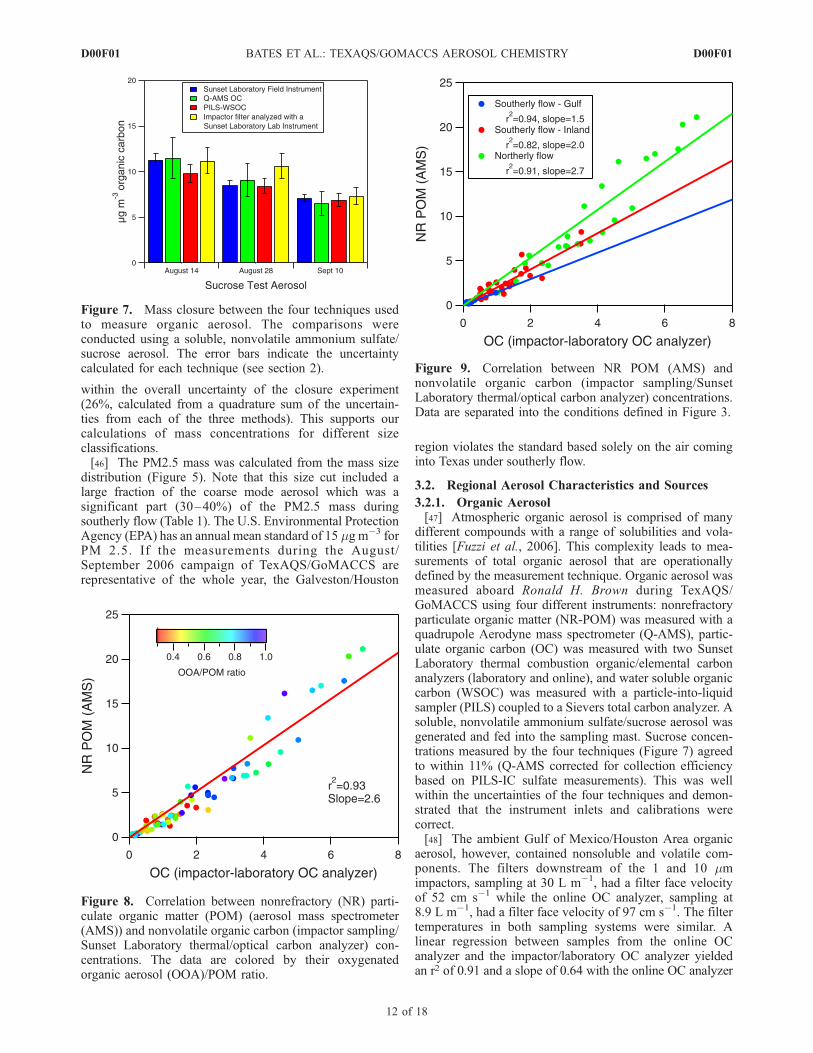
Figure 9. Correlation between NR POM (AMS) andnonvolatile organic carbon (impactor sampling/SunsetLaboratory thermal/optical carbon analyzer) concentrations.Data are separated into the conditions defined in Figure 3.


12 of 18

D00F01

results consistently less than the impactor/laboratory OCanalyzer. As both sampling systems used identical denuderswith flows of 30 L m�1, we conclude that the lower valuesobtained with the online OC analyzer were due to a higher lossof semivolatile organic carbon (SVOC) from the filter duringsampling. Similar losses have been documented by Eatoughet al. [2003]. Attempts to quantify the SVOC downstream ofthe online OC analyzer filter were unsuccessful (carbonimpregnated filter downstream of the particle filter). Thismay be in part due to the very high concentrations of VOCsin this area [Jobson et al., 2004]. If the denuders passed even1%of theVOCs, the signalmeasured as SVOCdownstream ofthe OC filter would be much greater than the particulate OC.[49] A linear regression between NR-POM and OC

(impactor/laboratory OC analyzer) concentrations yieldedan r2 of 0.93 and a slope of 2.6 (Figure 8). This NR-POM/OC ratio is higher than typically observed in urban or ruralareas (1.6 to 2.0 [Turpin and Lim, 2001]) and indicateseither a highly oxidized aerosol or a loss of SVOC duringimpactor sampling. Samples with a high NR-POM/OC ratiodidnotnecessarilyhaveahighOOA/NR-POMratio (Figure8)and the OOA/NR-POM ratios reported here are very similarto that found in other areas of the Northern Hemisphere[Zhang et al., 2007]. The highest NR-POM/OC ratioswere found in the samples collected during northerly flow(Figure 9) when the ship was located in the Houston ShipChannel very close to industrial sources of organic gases.The loss of OC from these samples during denuder/filtersample collection is consistent with gas-particle partitioningof secondary organic aerosol (SOA) and has been discussedpreviously by Eatough et al. [2003]. SOA forms from thecondensation of semivolatile reaction products of gasphase precursors. This partitioning is a reversible processas has been shown in the formation and evaporation ofSOA from a-pinene [Grieshop et al., 2007]. SOA can alsoform when semivolatile primary organic aerosol evaporates,oxidizes, and recondenses in the atmosphere [Robinson et al.,

2007]. This partitioning and photochemical processingcreates a regionally distributed organic aerosol as opposedto readily defined plumes from distinct sources. Thispartitioning also leads to negative artifacts in traditionaldenuder/filter sampling. We hypothesize that the highNR-POM/OC ratios observed in this study region are a resultof reevaporation of the SVOC from the filter.[50] A NR-POM/OC ratio can also be estimated based on

the AMS data alone [Aiken et al., 2008]. Using the m/z of44 as a surrogate for the oxygen content of POM and the m/z44, POM, OC relationships described by Aiken et al. [2008],the NR-POM/OC ratio during TexAQS averaged 1.86 ± 0.17.This ratio is typical of that found in urban and rural areas[Turpin and Lim, 2001].[51] A linear regression between NR-POM and WSOC

concentrations yielded an r2 of 0.76 and a slope of 3.2(Figure 10). Correlations of OOA and HOA with WSOCyielded r2 values of 0.67 and 0.15 and slopes of 2.6 and0.47, respectively. The NR-POM/WSOC slope of 3.2 isvery similar to that reported for the Gulf of Maine (3.3) [deGouw et al., 2007] and the OOA/WSOC slope of 2.6 isslightly less than that reported for Tokyo (3.2) [Kondo et al.,2007]. With a NR-POM/OC ratio of 1.6 to 2.0 [Turpin andLim, 2001], 49–62% of the NR-POM was water soluble.This is within the range of values (48–77%) measuredduring the summer months in other areas [Zappoli et al.,1999; Decesari et al., 2001; Sullivan et al., 2004; Jaffrezo etal., 2005] With an OOA/OC ratio of 2.2 [Zhang et al., 2005;Kondo et al., 2007], 85% of the OOA was water solubleduring TexAQS/GoMACCS.[52] The diurnal cycles of HOA and OOA concentrations

provide insights into the processes controlling their concen-trations in the boundary layer. HOA concentrations havebeen shown to correlate with CO mixing ratios [Allan et al.,2003; Zhang et al., 2005] and other markers of automobileexhaust emissions. Although this correlation was weak inthe Galveston/Houston region (r2 = 0.19) presumably from

Figure 10. Correlation between and NR POM and water soluble organic compound.


13 of 18

D00F01

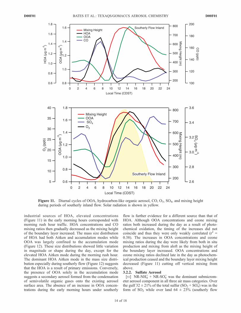
industrial sources of HOA, elevated concentrations(Figure 11) in the early morning hours corresponded withmorning rush hour traffic. HOA concentrations and COmixing ratios then gradually decreased as the mixing heightof the boundary layer increased. The mass size distributionof HOA had both Aitken and accumulation modes whileOOA was largely confined to the accumulation mode(Figure 12). These size distributions showed little variationin magnitude or shape during the day, except for theelevated HOA Aitken mode during the morning rush hour.The dominant HOA Aitken mode in the mass size distri-bution especially during southerly flow (Figure 12) suggeststhat the HOA is a result of primary emissions. Conversely,the presence of OOA solely in the accumulation modesuggests a secondary aerosol formed from the condensationof semivolatile organic gases onto the existing aerosolsurface area. The absence of an increase in OOA concen-trations during the early morning hours under southerly

flow is further evidence for a different source than that ofHOA. Although OOA concentrations and ozone mixingratios both increased during the day as a result of photo-chemical oxidation, the timing of the increases did notcoincide and thus they were only weakly correlated (r2 =0.38). The increases in OOA concentrations and ozonemixing ratios during the day were likely from both in situproduction and mixing from aloft as the mixing height ofthe boundary layer increased. OOA concentrations andozone mixing ratios declined late in the day as photochem-ical production ceased and the boundary layer mixing heightdecreased (Figure 11) cutting off vertical mixing fromabove.3.2.2. Sulfate Aerosol[53] NR-NH4

+ + NR-SO4= was the dominant submicrom-

eter aerosol component in all three air mass categories. Overthe gulf 32 ± 21% of the total sulfur (SO2 + SO4

=) was in theform of SO2 while over land 64 ± 23% (southerly flow

Figure 11. Diurnal cycles of OOA, hydrocarbon-like organic aerosol, CO, O3, SO4, and mixing heightduring periods of southerly inland flow. Solar radiation is shown in yellow.


14 of 18

D00F01

inland) and 55 ± 25% (northerly flow) of the total sulfur wasin the form of SO2. Large SO2 sources within the Houston/Galveston region include the Parish power plant (a coal-fired and natural gas-fired electric generation facility with

no SO2 gas scrubbers located in open farmland southwest ofHouston), fossil fuel-fired electrical generation and processheat facilities along the Houston Ship Channel, and isolatedlarge petrochemical complexes south of Houston [Brock etal., 2003]. The petrochemical industries located along theHouston Ship Cannel and the Parish power plant wereshown to be the predominant source of particle volume(mass) downwind of the Houston metropolitan area in 2000[Brock et al., 2003]. Particle number concentrations peakedimmediately downwind of the sources while particle vol-ume concentrations increased with distance from the sourceas SO2 and other gases were oxidized to form aerosol mass[Brock et al., 2003]. In a similar fashion, under northerlyflow conditions during TexAQS/GOMACCS, the largepoint sources of SO2 to the north of Houston and to theeast and south of Dallas (e.g., Big Brown, Martin Lake, andMonticello electrical stations) could easily account for theNR-SO4

= concentrations (7.4 ± 4.8 mg m�3) measuredaboard the ship. The transit times on the order of 1–2 dayswould permit a large fraction of the emitted SO2 to beconverted to sulfate. During southerly flow inland periods(category 2), the SO2 to total sulfur ratio was high, reflect-ing the local SO2 sources. The NR-SO4

= concentrations(3.2 ± 2.4 mg m�3), however, were only slightly higherthan that measured over the Gulf (2.5 ± 1.1 mg m�3) sincethe locally emitted SO2 was too freshly emitted to haveformed appreciable sulfate. The diurnal cycle of NR-SO4

=

during the southerly flow inland periods was similar to thatof OOA (Figure 11), decreasing during the night in theshallow stable boundary layer, increasing midmorning asthe convective mixing of the boundary layer increased andthen reaching an initial peak as the mixing height began todecrease late afternoon. Unlike OOA, however, the NR-SO4

=

concentrations increased late in the day. We hypothesizethat this is a result of advection of sulfate that was producedover the Gulf during the afternoon. A similar increase is notseen in ozone or OOA since their precursors were notabundant in the onshore flow.[54] A key question, then, is what is the source of the

elevated SO2 and sulfate concentrations over the Gulf ofMexico in the ‘‘background’’ air (category 1) enteringTexas? Biogenic dimethyl sulfide concentrations in thesurface seawater off the coast of Texas averaged 2.4 ±0.95 nM L�1, a value typical of this latitude during thesummer [Bates et al., 1987]. Using the wind speeds mea-sured at the ship and the Nightingale et al. [2000] windspeed/transfer velocity relationship, the flux of DMS to theatmosphere was 3.2 ± 2.6 mM m�2d. Over the backgroundmarine atmosphere this flux supports an atmospheric sulfateconcentration of 0.2–0.4 mg m�3 [Bates et al., 2001], farless than that measured over the Gulf of Mexico. Anotherpotential source of sulfate is the African continent as theseair masses did contain high concentrations of dust. How-ever, sulfate concentrations measured with dust in thesubmicrometer aerosol outflow of Africa were only 5–11% of the dust concentrations [Bates et al., 2001; Formentiet al., 2003], far less than that measured over the Gulf ofMexico. CO mixing ratios in this air mass (81 ± 14 ppbv)also suggest an absence of forest fire or urban pollution. Athird potential source of sulfate is volcanic emissions. TheFLEXPART back trajectories showed that some air massessampled at the ship traveled through the Caribbean Sea and

Figure 12. Mass size distributions of the dominant NRaerosol components measured by the quadrupole aerosolmass spectrometer.


15 of 18

D00F01

may have passed over the Soufriere Hills Volcano onMontserrat Island. During July–September 2006 the aver-age sulfur dioxide flux from the volcano was 200 t per day(The Montserrat Volcano Observatory, http://www.mvo.ms/)at an elevation of 1.1 km. While some of this SO2 may havebeen mixed down into the marine boundary layer most of itwill be transported in the free troposphere. There was nocorrelation of atmospheric sulfate concentrations measured atthe ship with trajectories that had passed over MontserratIsland.[55] A fourth potential source of the sulfate over the Gulf

of Mexico is from marine vessel emissions. Emissions frommarine vessels have gained increasing attention due to theirsignificant local, regional, and global effects [Corbett et al.,2007]. The corridor from the entrance to the Gulf of Mexicoto Louisiana/Texas is a major shipping lane serving the Portof South Louisiana (New Orleans) and the Port of Houston,two of the ten busiest ports in the world by cargo volume(Gulf of Mexico Program, U.S. Environmental ProtectionAgency, http://epa.gov/gmpo/index.html). Recent shipemission inventories list the U.S. Gulf Coast emissions at100,000 t of SO2 per year [Wang et al., 2008]. If this SO2 isemitted into a 500m marine boundary layer over an area of500,000 km2 (a 200 nautical mile swath through the Gulf ofMexico to the Texas/Louisiana coast), with an atmosphericsulfur aerosol lifetime of one week, it would generate aconcentration of 12 mg m�3, more than 4 times the averageconcentration measured over the Gulf. The resulting aerosolwould be acidic (measured ammonium to sulfate molar ratiowas 0.79 ± 0.42) since the only source of ammonium ion isthe ammonia emitted from the ocean [Quinn et al., 1990].Ship emissions also include high concentrations of nitrogenoxides (174,000 t expressed as NO2 per year over the U.S.Gulf Coast) [Wang et al., 2008]. Over the ocean, nitrogenoxides and their reaction products are absorbed onto theexisting aerosol surface area and are thus generally found inthe supermicrometer aerosol associated with dust or sea salt[Bates et al., 2004]. The supermicrometer aerosol measuredover the Gulf of Mexico was highly enriched in nitrate (15%of the total mass) and both the submicrometer and super-micrometer seasalt aerosols were depleted in chloride fromthe reaction with sulfuric and nitric acid vapors [Bates et al.,2004]. Ship emissions, therefore, appear to be the majorsource of sulfate and nitrate over the Gulf of Mexico duringTexAQS/GoMACCS.

4. Conclusions

[56] During most of August 2006, the boundary layeraerosol over the NW Gulf of Mexico advected intothe region from the south and consisted of submicrometer(6.5 mg m�3) NR-SO4

= and dust and supermicrometer(17.2 mg m�3) sea salt and dust. Although this air masshad been over the Atlantic Ocean/Gulf of Mexico for 1–2 weeks, it was heavily impacted by continental (Saharandust) and anthropogenic (ship) emissions. As the air massentered southern Texas, local sources added an Aitken modeHOA rich aerosol. OOA and NR-SO4

= concentrations inlandwere lowest in the shallow, stable nocturnal boundary layerand increased during the day as the boundary layer mixingheight increased, reflecting their secondary source. HOAconcentrations and CO mixing ratios followed the opposite

pattern, reflecting their primary source. Concentrations werehighest in the early morning when the source was strong(automobile traffic) and mixing was limited (shallow, stableboundary layer) and then decreased during the day as theboundary layer mixing height increased.[57] During September 2006 the boundary layer aerosol

over southern Texas and the NW Gulf of Mexico advectedinto the region from the north and consisted of submicrom-eter (20.8 mg m�3) NR-SO4

= and NR-POM and supermi-crometer (7.4 mg m�3) POM and dust.[58] The integrated PM 2.5 mass at ambient RH includes

the accumulation mode (primarily acidic sulfate and dustunder southerly flow conditions) and part of the coarsemode (primarily sea salt, dust, and the acidic nitrate andsulfate absorbed by these basic components). The averagePM 2.5 mass advecting into the Houston-Galveston areafrom the south during TexAQS 2006 was 20 ± 12 mg m�3.Air quality forecast models need to include ship emissionsand dust transport to correctly characterize aerosol loadingsin SE Texas. Compliance with PM 2.5 regulations in theHouston-Galveston area may require stricter controls onupwind aerosol sources (e.g., ship emissions).

[59] Acknowledgments. We thank the officers and crewofNOAAR/VRonald H. Brown for their cooperation and enthusiasm and D. Hamilton,T.B. Onasch, J.D. Allan, and D.R. Worsnop for technical support. We thankJ. Meagher, F. Fehsenfeld, and A.R. Ravishankara for programmaticsupport. This research was funded by the Atmospheric Constituents Projectof the NOAA Climate and Global Change Program, the NOAA Office ofOceanic and Atmospheric Research, the NOAA Health of the AtmosphereProgram and the Texas Air Quality Study. This is NOAA/PMEL contribu-tion 3139.

ReferencesAiken, A. C., et al. (2008), O/C and OM/OC ratios of primary, secondary,and ambient organic aerosols with high resolution time-of-flight aerosolmass spectrometry, Environ. Sci. Technol., 42, 4478–4485.

Allan, J. D., J. L. Jimenez, P. I. Williams, M. R. Alfarra, K. N. Bower, J. T.Jayne, H. Coe, and D. R. Worsnop (2003), Quantitative sampling usingan Aerodyne aerosol mass spectrometer: 1. Techniques of data interpreta-tion and error analysis, J. Geophys. Res., 108(D3), 4090, doi:10.1029/2002JD002358.

Bates, T. S., J. D. Cline, R. H. Gammon, and S. Kelly-Hansen (1987),Regional and seasonal variations in the flux of oceanic dimethylsulfideto the atmosphere, J. Geophys. Res., 92, 2930–2938, doi:10.1029/JC092iC03p02930.

Bates, T. S., P. K. Quinn, D. J. Coffman, J. E. Johnson, T. L. Miller, D. S.Covert, A. Wiedensohler, S. Leinert, A. Nowak, and C. Neusuß (2001),Regional physical and chemical properties of the marine boundary layeraerosol across the Atlantic during Aerosols99: An overview, J. Geophys.Res., 106, 20,767–20,782, doi:10.1029/2000JD900578.

Bates, T. S., D. J. Coffman, D. S. Covert, and P. K. Quinn (2002), Regionalmarine boundary layer aerosol size distributions in the Indian, Atlantic, andPacific Oceans: A comparison of INDOEX measurements with ACE-1,ACE-2, and Aerosols99, J. Geophys. Res., 107(D18), 8026, doi:10.1029/2001JD001174.

Bates, T. S., et al. (2004), Marine boundary layer dust and pollutiontransport associated with the passage of a frontal system over easternAsia, J. Geophys. Res., 109, D19S19, doi:10.1029/2003JD004094.

Bates, T. S., P.K.Quinn,D. J. Coffman, J. E. Johnson, andA.M.Middlebrook(2005), The dominance of organic aerosols in the marine boundary layerover the Gulf of Maine during NEAQS 2002 and their role in aerosol lightscattering, J. Geophys. Res., 110, D18202, doi:10.1029/2005JD005797.

Berner, A., C. Lurzer, F. Pohl, O. Preining, and P. Wagner (1979), The sizedistribution of the urban aerosol in Vienna, Sci. Total Environ., 13, 245–261, doi:10.1016/0048-9697(79)90105-0.

Brock, C. A., et al. (2003), Particle growth in urban and industrial plumes inTexas, J. Geophys. Res., 108(D3), 4111, doi:10.1029/2002JD002746.

Cahill, T. A., R. A. Eldred, and P. J. Feeney (1986), Particulate monitoringand data analysis for the National Park Service, 1982–1985, Air Qual.Group, Crocker Nucl. Lab., Davis, Calif.


16 of 18

D00F01

Carrico, C. M., P. Kus, M. J. Rood, P. K. Quinn, and T. S. Bates (2003),Mixtures of pollution, dust, seasalt and volcanic aerosol during ACE-Asia:Light scattering properties as a function of relative humidity, J. Geophys.Res., 108(D23), 8650, doi:10.1029/2003JD003405.

Cheng, Y., B. Chen, H. Yeh, I. Marshall, J. Mitchell, andW. Griffeths (1993),Behavior of compact nonspherical particles in the TSI aerodynamic particlesizer model APS33B-Ultra-stokesian drag forces, Aerosol Sci. Technol.,19, 255–267, doi:10.1080/02786829308959634.

Corbett, J. J., J. J. Winebrake, E. H. Green, P. Kasibhatla, V. Eyring, andA. Lauer (2007), Mortality from ship emissions: A global assessment,Environ. Sci. Technol., 41(24), 8512–8518, doi:10.1021/es071686z.

Decesari, S., M. C. Facchini, E. Matta, F. Lettini, M. Mircea, S. Fuzzi,E. Tagliavini, and J. P. Putaud (2001), Chemical features and seasonalvariation of fine aerosol water-soluble organic compounds in the Po Valley,Italy, Atmos. Environ., 35, 3691–3699, doi:10.1016/S1352-2310(00)00509-4.

de Gouw, J. A., et al. (2007), Sources of particulate matter in the North-eastern United States: 1. Direct emissions and secondary formation oforganic matter in urban plumes, J. Geophys. Res., 113, D08301,doi:10.1029/2007JD009243.

Eatough, D. J., R. W. Long, W. K. Modey, and N. L. Eatough (2003), Semi-volatile secondary organic aerosol in urban atmospheres: Meeting ameasurement challenge, Atmos. Environ., 37, 1277–1292, doi:10.1016/S1352-2310(02)01020-8.

Feely, R. A., G. J. Massoth, and G. T. Lebon (1991), Sampling of marineparticulate matter and analysis by X-ray fluorescence spectrometry, inMarine Particles: Analysis and Characterization, Geophys. Monogr.Ser, vol. 63, edited by D. C. Hurd and D. W. Spencer, pp. 251–257,AGU, Washington, DC.

Formenti, P., W. Elbert, W. Maenhaut, H. Haywood, and M. O. Andreae(2003), Chemical composition of mineral dust aerosol during the SaharanDust Experiment (SHADE) airborne campaign in the Cape Verde region,September 2000, J. Geophys. Res., 108(D18), 8576, doi:10.1029/2002JD002648.

Fuzzi, S., et al. (2006), Critical assessment of the current state of scientificknowledge, terminology, and research needs concerning the role oforganic aerosols in the atmosphere, climate, and global change, Atmos.Chem. Phys., 6, 2017–2038.

Gerbig, C., S. Schmitgen, D. Kley, A. Volz-Thomas, K. Dewey, andD. Haaks(1999), An improved fast-response vacuum-UV resonance fluorescenceCO instrument, J. Geophys. Res., 104(D1), 1699–1704, doi:10.1029/1998JD100031.

Grieshop, A. P., N. M. Donahue, and A. L. Robinson (2007), Is the gas-particle partitioning in alpha-pinene secondary organic aerosol reversible?,Geophys. Res. Lett., 34, L14810, doi:10.1029/2007GL029987.

Grund, C. J., R. M. Banta, J. L. George, J. N. Howell, M. J. Post, R. A.Richter, and A. M. Weickmann (2001), High-resolution doppler lidar forboundary layer and cloud research, J. Atmos. Oceanic Technol., 18, 376–393, doi:10.1175/1520-0426(2001)018<0376:HRDLFB>2.0.CO;2.

Harrison, R. M., and J. Yin (2000), Particulate matter in the atmosphere:Which particle properties are important for its effects on health?, Sci.Total Environ., 249, 85–101, doi:10.1016/S0048-9697(99)00513-6.

Holland, H. D. (1978), The Chemistry of the Atmosphere and Oceans, 154pp., John Wiley, New York.

Huffman, J. A., J. T. Jayne, F. Drewnick, A. C. Aiken, T. Onasch, D. R.Worsnop, and J. L. Jimenez (2005), Design, Modeling, Optimization, andExperimental Tests of a Particle Beam Width Probe for the AerodyneAerosol Mass Spectrometer, Aerosol Sci. Technol., 39, 1143–1163,doi:10.1080/02786820500423782.

Intergovernmental Panel on Climate Change (IPCC) (2007), ClimateChange 2007: The Physical Science Basis. Contribution of WorkingGroup I to the Fourth Assessment Report of the Intergovernmental Panelon Climate Change, edited by S. Solomon et al., Cambridge Univ. Press,Cambridge, U.K.

Jaffrezo, J.-L., G. Aymoz, C. Delaval, and J. Cozic (2005), Seasonal varia-tions of the water soluble organic carbon mass fraction of aerosol in twovalleys of the French Alps, Atmos. Chem. Phys., 5, 2809–2821.

Jayne, J. T., D. C. Leard, X. Zhang, P. Davidovits, K. A. Smith, C. E. Kolb,and D. R. Worsnop (2000), Development of an aerosol mass spectrometerfor size and composition analysis of submicron particles, Aerosol Sci.Technol., 33, 49–70, doi:10.1080/027868200410840.

Jimenez, J. L., et al. (2003), Ambient aerosol sampling using the AerodyneAerosol Mass Spectrometer, J. Geophys. Res., 108(D7), 8425,doi:10.1029/2001JD001213.

Jobson, B. T., C. M. Berkowitz, W. C. Kuster, P. D. Goldan, E. J. Williams,F. C. Fesenfeld, E. C. Apel, T. Karl, W. A. Lonneman, and D. Riemer(2004), Hydrocarbon source signatures in Houston, Texas: Influence ofthe petrochemical industry, J. Geophys. Res., 109, D24305, doi:10.1029/2004JD004887.

Kondo, Y., Y. Miyazaki, N. Takegawa, T. Miyakawa, R. J. Weber, J. L.Jimenez, Q. Zhang, and D. R. Worsnop (2007), Oxygenated and water-soluble organic aerosols in Tokyo, J. Geophys. Res., 112, D01203,doi:10.1029/2006JD007056.

Lanz, V. A., M. R. Alfarra, U. Baltensperger, B. Buchmann, C. Hueglin,and A. S. H. Prevot (2007), Source apportionment of submicron organicaerosols at an urban site by factor analytical modelling of aerosol massspectra, Atmos. Chem. Phys., 7, 1503–1522.

Mader, B. T., et al. (2003), Sampling methods used for the collection ofparticle-phase organic and elemental carbon during ACE-Asia, Atmos.Environ., 37(11), 1435–1449, doi:10.1016/S1352-2310(02)01061-0.

Malm, W. C., J. F. Sisler, D. Huffman, R. A. Eldred, and T. A. Cahill(1994), Spatial and seasonal trends in particle concentration and opticalextinction in the United States, J. Geophys. Res., 99, 1347–1370,doi:10.1029/93JD02916.

Marshall, I. A., J. P. Mitchell, and W. D. Griffiths (1991), The behavior ofregular-shaped non-spherical particles in a TSI Aerodynamic ParticleSizer, J. Aerosol Sci., 22, 73–89, doi:10.1016/0021-8502(91)90094-X.

Matthew, B. M., T. B. Onasch, and A. M. Middlebrook (2008), Collectionefficiencies in an Aerodyne aerosol mass spectrometer as a function ofparticle phase for laboratory generated aerosols, Aerosol Sci. Technol., inpress.

Nightingale, P. D., P. S. Liss, and P. Schlosser (2000), Measurements of air-sea gas transfer during an open ocean algal bloom, Geophys. Res. Lett.,27, 2117–2120, doi:10.1029/2000GL011541.

Orsini, D. A., Y. Ma, A. Sullivan, B. Sierau, K. Baumann, and R. J. Weber(2003), Refinements to the particle-into-liquid sampler (PILS) for groundand airborne measurements of water-soluble aerosol composition, Atmos.Environ., 37, 1243–1259, doi:10.1016/S1352-2310(02)01015-4.

Perry, K. D., T. A. Cahill, R. A. Eldred, D. D. Dutcher, and T. E. Gill(1997), Long-range transport of North African dust to the eastern UnitedStates, J. Geophys. Res., 102, 11,225–11,238, doi:10.1029/97JD00260.

Quinn, P. K., and D. J. Coffman (1998), Local closure during ACE 1:Aerosol mass concentration and scattering and backscattering coeffi-cients, J. Geophys. Res., 103, 16,575–16,596, doi:10.1029/97JD03757.

Quinn, P. K., T. S. Bates, J. E. Johnson, D. S. Covert, and R. J. Charlson(1990), Interactions between the sulfur and reduced nitrogen cyclesover the central Pacific Ocean, J. Geophys. Res., 95, 16,405–16,416.

Quinn, P. K., D. J. Coffman, V. N. Kapustin, T. S. Bates, and D. S. Covert(1998), Aerosol optical properties in the marine boundary layer duringACE 1 and the underlying chemical and physical aerosol properties,J. Geophys. Res., 103, 16,547–16,563, doi:10.1029/97JD02345.

Quinn, P. K., et al. (2000), Surface submicron aerosol chemical composi-tion: What fraction is not sulfate?, J. Geophys. Res., 105, 6785–6806.

Quinn, P. K., D. J. Coffman, T. S. Bates, T. L. Miller, J. E. Johnson, E. J.Welton, C. Neususs, M. Miller, and P. Sheridan (2002), Aerosoloptical properties during INDOEX 1999: Means, variabilities, andcontrolling factors, J. Geophys. Res., 107(D19), 8020, doi:10.1029/2000JD000037.

Quinn, P. K., et al. (2004), Aerosol optical properties measured on board theRonald H. Brown during ACE-Asia as a function of aerosol chemicalcomposition and source region, J. Geophys. Res., 109, D19S01,doi:10.1029/2003JD004010.

Robinson, A. L., M. M. Donahue, M. K. Shrivastava, E. A.Weitkamp, A. M.Sage, A. P. Grieshop, T. E. Lane, J. R. Pierce, and S. N. Pandis (2007),Rethinking organic aerosols: Semivolatile emissions and photochemicalaging, Science, 315, 1259–1262, doi:10.1126/science.1133061.

Savoie, D. L., and J. M. Prospero (1980), Water-soluble potassium, calcium,andmagnesium in the aerosols over the tropical NorthAtlantic, J. Geophys.Res., 85, 385–392, doi:10.1029/JC085iC01p00385.

Schauer, J. J., et al. (2003), ACE Asia intercomparison of a thermal-opticalmethod for the determination of particle-phase organic and elementalcarbon, Environ. Sci. Technol., 37, 993–1001, doi:10.1021/es020622f.

Schindler, D. W., S. E. M. Kasian, and R. H. Hessiein (1989), Biologicalimpoverishment in lakes of the midwestern and northeastern UnitedStates from acid rain, Environ. Sci. Technol., 23 , 573 – 580,doi:10.1021/es00063a010.

Seibert, P., and A. Frank (2004), Source-receptor matrix calculation with aLagrangian particle dispersion model in backward mode, Atmos. Chem.Phys., 4, 51–63.

Stohl, A., and D. J. Thomson (1999), A density correction for Lagrangianparticle dispersion models, Boundary Layer Meteorol., 90, 155–167,doi:10.1023/A:1001741110696.

Stohl, A., M. Hittenberger, and G. Wotawa (1998), Validation of theLagrangian particle dispersion model FLEXPART against large scaletracer experiments, Atmos. Environ., 32, 4245–4264, doi:10.1016/S1352-2310(98)00184-8.

Sullivan, A. P., R. J. Weber, A. L. Clements, J. R. Turner, M. S. Bae, and J. J.Schauer (2004), A method for on-line measurement of water-soluble


17 of 18

D00F01

organic carbon in ambient aerosol particles: Results from an urban site,Geophys. Res. Lett., 31, L13105, doi:10.1029/2004GL019681.

Sullivan, A. P., R. E. Peltier, C. A. Brock, J. A. de Gouw, J. S. Holloway,C.Warneke, A. G.Wollny, andR. J.Weber (2006), Airbornemeasurementsof carbonaceous aerosol soluble in water over northeastern United States:Method development and an investigation into water-soluble organiccarbon sources, J. Geophys. Res., 111, D23S46, doi:10.1029/2006JD007072.

Turpin, B. J., and H. Lim (2001), Species contribution to PM2.5 concen-trations: Revisiting common assumptions for estimating organic mass,Aerosol Sci. Technol., 35, 602–610, doi:10.1080/02786820152051454.

Ulbrich, I. M., M. R. Canagaratna, Q. Zhang, D. R. Worsnop, and J. L.Jimenez (2008), Interpretation of organic components from positivematrix factorization of aerosol mass spectrometric data, Atmos. Chem.Phys. Discuss., 8, 6729–6791.

Wang, C., J. J. Corbett, and J. Firestone (2008), Improving spatialrepresentation of global ship emissions inventories, Environ. Sci.Technol., 42, 193–199, doi:10.1021/es0700799.

Weber, R. J., D. Orsini, Y. Daun, Y.-N. Lee, P. Klotz, and F. Brechtel(2001), A particle-in-liquid collector for rapid measurement of aerosolchemical composition, Aerosol Sci. Technol., 35, 718–727, doi:10.1080/02786820152546761.

Whittlestone, S., and W. Zahorowski (1998), Baseline radon detectors forship-board use: Development and deployment in ACE-1, J. Geophys.Res., 103, 16,743–16,751, doi:10.1029/98JD00687.

Winklmayr, W., G. P. Reischl, A. O. Lindner, and A. Berner (1991),New electromobility spectrometer for the measurement of aerosol sizedistributions in the size range 1 to 1000 nm, J. Aerosol Sci., 22, 289–296,doi:10.1016/S0021-8502(05)80007-2.

Zappoli, S., et al. (1999), Inorganic, organic and macromolecularcomponents of fine aerosol in different areas of Europe in relation totheir water solubility, Atmos. Environ., 33, 2733–2743, doi:10.1016/S1352-2310(98)00362-8.

Zhang, Q., M. R. Alfarra, D. R. Worsnop, J. D. Allan, H. Coe, M. R.Canagaratna, and J. L. Jimenez (2005), Deconvolution and quantificationof hydrocarbon-like and oxygenated organic aerosols based on aerosolmass spectrometry, Environ. Sci. Technol., 39, 4938–4952, doi:10.1021/es048568l.

Zhang, Q., et al. (2007), Ubiquity and dominance of oxygenated species inorganic aerosols in anthropogenically-influenced Northern Hemispheremidlatitudes, Geophys. Res. Lett., 34 , L13801, doi:10.1029/2007GL029979.

��W. M. Angevine, W. A. Brewer, B. L. Lerner, S. C. Tucker, and E. J.

Williams, Chemical Sciences Division, Earth Systems Research Laboratory,NOAA, Boulder, CO 80309-0216, USA.T. S. Bates, D. Coffman, P. K. Quinn, and K. Schulz, Pacific Marine

Environmental Laboratory, NOAA, 7600 Sand Point Way NE, Building 3,Seattle, WA 98115, USA. ([email protected])D. S. Covert and J. E. Johnson, Joint Institute for the Study of the

Atmosphere and Ocean, University of Washington, Box 355672, Seattle,WA 98195, USA.A. Stohl, Department of Regional and Global Pollution Issues,

Norwegian Institute for Air Research, P. O. Box 100, N-2027 Kjeller,Norway.


18 of 18

D00F01

Documents

Boundary layer aerosol chemistry during TexAQS/GoMACCS - NILU