Embed Size (px)
Citation preview
Journal of Computational Physics169,302–362 (2001)
doi:10.1006/jcph.2000.6626, available online at http://www.idealibrary.com on
Boundary Integral Methods forMulticomponent Fluids and
Multiphase Materials
T. Y. Hou,∗ J. S. Lowengrub,† and M. J. Shelley‡∗Department of Applied Mathematics, California Institute of Technology, Pasadena, California 91125;†School of Mathematics, University of Minnesota, Minneapolis, Minnesota 55455; and Department
of Mathematics, University of North Carolina, North Carolina 27599; and‡Courant Instituteof Mathematical Sciences, New York University, New York, New York 10012
E-mail: [email protected]
Received March 13, 2000; revised August 24, 2000
We present a brief review of the application of boundary integral methods in twodimensions to multicomponent fluid flows and multiphase problems in materialsscience. We focus on the recent development and outcomes of methods which accu-rately and efficiently include surface tension. In fluid flows, we examine the effectsof surface tension on the Kelvin–Helmholtz and Rayleigh–Taylor instabilities in in-viscid fluids, the generation of capillary waves on the free surface, and problemsin Hele-Shaw flows involving pattern formation through the Saffman–Taylor insta-bility, pattern selection, and singularity formation. In materials science, we discussmicrostructure evolution in diffusional phase transformations, and the effects of thecompetition between surface and elastic energies on microstructure morphology. Acommon link between these different physical phenomena is the utility of an analysisof the appropriate equations of motion at small spatial scales to develop accurate andefficient time-stepping methods.c© 2001 Academic Press
1. INTRODUCTION
The past 15 years have seen the rapid development of numerical methods, especially intwo dimensions, for applying boundary integral methods to multifluid problems in fluiddynamics, and more recently to multiphase problems in materials science. By multifluidor multiphase we mean systems where the constitutive properties of the fluid or materialchange abruptly at a dividing interface. The case of immiscible fluids, such as oil andwater, stands as the classical example. An important complicating property of such systemsis surface tension (or surface energy in the materials context). Much recent effort in theapplication of boundary integral methods has focused on developing numerical methods
302
0021-9991/01 $35.00Copyright c© 2001 by Academic PressAll rights of reproduction in any form reserved.
BOUNDARY INTEGRAL METHODS 303
that efficiently and accurately include surface tension. And while boundary integral methodsare applicable only to a restricted type of flow problem, these problems are central influids and materials science. In fluids, these problems include those producing prototypepatterns, the first nonlinear stages of immiscible fluids mixing, the development of finite-time singularities, and capillary wave generation in water waves. In materials science, theseproblems include morphology selection in phase–transition dynamics and many-precipitatecoarsening, under various types of material anisotropy.
In this paper, we review recent applications of boundary integral methods to simulateinterfacial dynamics of multicomponent fluids and multiphase materials with surface tensionin two dimensions. A boundary integral representation applies when, for example, thepartial differential equations (PDEs) governing the bulk fluid or material are piecewisehomogeneous, and for which a Green’s function can be found or approximated. In suchcases, the dynamics of the system can be reduced to the self-contained, nonlocal dynamicsof the interface separating the homogeneous fluids or phases. In fluid dynamics this typicallymeans that we are dealing with potential flows (e.g., inviscid and irrotational flows, Hele-Shaw flows) or Stokes flows. (Except in special cases we neglect the latter, as Stokes flowsare the subject of a separate review in this volume.) Boundary integral methods are not(immediately) applicable to more general interfacial fluid flows, such as those governedby the viscous Navier–Stokes equations. In the materials science context, we focus ondiffusional phase transformations whose formulation is closely related to that of Hele-Shawflows.
For a few specific problems in these areas, we present a historical perspective and thendiscuss what we believe to be the state of the art in numerical simulation. Because of thelimited scope of our review, we refer the reader to more general reviews of interfacial fluidflows by Hou [85], Hyman [88], Prosperetti and Oguz [145], Romate [158], Sarpkaya [166],Scardovelli and Zaleski [167], Schwarz and Fenton [170], Stone [180], Tsai and Yue [198],and Yeung [215]. For diffusional phase transformations in materials science, see the moregeneral reviews by Johnson and Voorhees [92], Purdy [150], and Voorhees [201, 202].
In addition, it is important to note that there are other, more general, numerical ap-proaches to simulating free boundary problems in fluids and materials. These include level-set, volume-of-fluid, immersed boundary, front-tracking, phase-field, and discrete atommethods. Several of these approaches are the subject of separate reviews in this volume,and here we focus exclusively on boundary integral methods. When applicable, boundary in-tegral methods outperform these other methodologies in accurately and efficiently capturingthe dynamics. And so, while being applicable to a core set of problems in fluid dynam-ics and materials, boundary integral methods provide excellent benchmark simulations forcomparing these different computational strategies.
There are several difficulties in including the effects of surface tension in a simulation.First, as the pressure jump due to surface tension at an interface is proportional to the in-terfacial curvature, a high number of spatial derivatives are introduced into the dynamics.This results in high-order constraints on explicit time-stepping methods. Second, seem-ingly natural choices of frame in which to compute the interfacial motion can make theseconstraints strongly time-dependent, and prohibitive. And third, due to the divergence freecondition on the fluid velocity, these curvature dependent terms enter the dynamics nonlo-cally and nonlinearly. Such difficulties are not specific to the inclusion of surface tension,but also arise when dealing with the dynamics of surfaces or curves that have elastic orother curvature-dependent responses.

304 HOU, LOWENGRUB, AND SHELLEY
Within the context of boundary integral methods for two-dimensional potential and Hele-Shaw flows, we show in HLS94 [81] how these difficulties arising from surface tension canbe subverted, and efficient and accurate numerical methods constructed. This relies inpart on the “small-scale decomposition” (SSD), a mathematical analysis which identifiesthe source of stiffness by examining the equations of motion at small length-scales. TheSSD analysis shows that when the equations of motion are properly formulated, surfacetension acts through a linear operator at small length-scales. This contribution can then betreated implicitly and efficiently in a time-integration scheme, and the high-order constraintsremoved. The consequent improvements in efficiency and results can be dramatic. Forexample, in HLS94 we simulated the very long-time development of densely branchedpatterns in radial Hele-Shaw flow, and suggested the formation of “topological singularities”in the Kelvin–Helmholtz problem with surface tension. This latter study was continued inHLS97 [82], where we developed nonuniform grid methods, used high-order time-stepping,and quantified many aspects of this singularity through careful numerical simulation. Herewe will review many other related efforts and works.
These analytical approaches might point the way to the development of similar meth-ods in more complicated situations. For example, simulations of heart function using theimmersed boundary method are currently constrained in time-step by the stiffness inducedby “fiber” elasticity, which is a curvature-dependent boundary force (C. Peskin, privatecommunication). In this situation, one must also consider the rotational and viscous aspectsof the fluid flow, set in a very complicated geometry.
In Section 2, we discuss the application of boundary integral methods to inviscid andincompressible multifluid flows with surface tension. The prototype problem is the non-linear development of the Kelvin–Helmholtz problem under surface tension. We discussextensions to the Rayleigh–Taylor instability and water waves. In Section 3, we discussthe application of boundary integral methods to Hele-Shaw flows, to the study of patternformation and morphology selection, and singularity formation. In Section 4, we discuss theapplication of boundary integral methods to diffusional phase transitions in materials sci-ence. Section 5 gives concluding remarks and discusses future directions in the applicationof boundary integral methods.
2. INVISCID INTERFACIAL FLUID FLOWS WITH SURFACE TENSION
In this section, we present a brief review of recent applications of boundary integralmethods to study inviscid, incompressible interfacial flows with surface tension in twodimensions. In particular, we focus on the nonlinear evolution of vortex sheets separatingtwo immiscible fluids and the dynamic generation of capillary waves on a free surface.
Many physically interesting fluid flows involve the motion of interfaces separating im-miscible flow components with small viscosity. In flows where there is rapid motion, theeffects of viscosity may be secondary in importance to those of surface tension. This is par-ticularly evident in shear flows [196]. Moreover, surface tension is central to understandingfluid dynamic phenomena such as droplet formation and capillary wave motion.
Surface tension at an interface separating two immiscible fluids arises due to an imbalanceof the fluid components’ intermolecular cohesive forces. It is modeled through the Laplace–Young condition, which relates the pressure jump across an interface to the interfacialcurvature. As mentioned in the Introduction, the accurate simulation of interfaces withsurface tension is a problem of considerable difficulty, and stable, efficient, and accurate
BOUNDARY INTEGRAL METHODS 305
boundary integral methods have been developed only recently. We review work that isrepresentative of the current state-of-the-art research in this field.
2.1. Historical Perspective
The use of boundary integral methods in inviscid interfacial flows in two dimensionshas a long and rich history that dates back to the 1932 study of vortex sheet roll-up byRosenhead [160]. Much later, Birkhoff [26] developed a boundary integral formulation formore general interfacial motion. In 1976, Longuet-Higgins and Cokelet [120] developed thefirst successful boundary integral method to compute plunging breakers. Since then, manyboundary integral methods have been developed to simulate free-surface Euler flows. See[5, 11, 13–19, 21, 22, 27, 33, 34, 43, 49, 53, 54, 64, 81, 82, 103–105, 132, 134, 147, 151,155, 156, 172, 197, 199, 200, 209, 214, 215, 220] for a small sample. For a more completeset of references, see the review articles listed in the Introduction and the references therein.While where as it is not our goal to review all of this work here, we point out that theorigins of many modern boundary integral algorithms can be traced to the seminal paperof Bakeret al. (BMO82) [14]. In that paper, a detailed derivation of the boundary integralequations is given and the use of iteration methods, to solve the resulting integral equations,is pioneered. BMO82 then applied the methods to study breaking waves over finite-bottomtopographies and interacting free-surface waves.
The study of interfacial flows with surface tension in two dimensions using boundaryintegral methods began with the work of Zalosh [218] in which the nonlinear evolution of avortex sheet was considered (density-matched components). Subsequently, other methodshave been developed for flows with different density flow components, by many othersincluding Baker and Moore [15], Boulton-Stone and Blake [27], Kudela [105], Pullin [149],Rangel and Sirignano [151], Robinson and Boulton-Stone [156], Rottman and Olfe [161],Tulin [199], and Yang [214].
All of the boundary integral methods listed exhibit numerical instability that requiressome type of ad-hoc numerical smoothing to yield smooth evolution. The primary diffi-culty with using smoothing is that it can lead to unphysical results because the effects ofsmoothing may dominate those of surface tension. In independent works, Bealeet al. [18,19, 22] and Baker and Nachbin (BN98) [11] identified certain incompatibilities in the spatialdiscretization of the boundary integral equations, both with and without surface tension.These incompatibilities were shown to lead to numerical instability of the type observed inprevious studies. Bealeet al. and BN98 presented alternative, highly accurate, and stablemethods.
Additional difficulties occur when the equations are discretized in time. The differentialclustering of interface grid points may result in prohibitive time-step restrictions for stabilityfor explicit time integration methods because of the high-order derivative terms introducedby surface tension. Because the surface tension appears in the equations nonlocally andnonlinearly, standard implicit time-stepping methods are very expensive. To overcome thesedifficulties, Hou, Lowengrub, and Shelley (HLS94, HLS97) [81, 82] derived an alternateformulation of the equations which has all the nice properties for time integration schemesthat are associated with having a linear highest order term (such as diffusion term in theNavier–Stokes equations). For example, the methods given in HLS94 and HLS97 are explicitin Fourier space and do not have the severe time-step restrictions usually associated withsurface tension. The methods are then used to study the nonlinear, long-time evolution of
306 HOU, LOWENGRUB, AND SHELLEY
vortex sheets with surface tension, interfaces between fluid components with small densitydifferences (Boussinesq approximation) and Hele-Shaw interfaces.
Later, Ceniceros and Hou (CH98) [33] proved convergence of a semidiscrete (time-continuous) version of the methods proposed in HLS94/HLS97 for general two-fluid inter-facial flows. CH98 also carefully investigated the effects of surface tension on the Rayleigh–Taylor instability. In addition, Ceniceros and Hou (CH99a) [34] applied the methods ofHLS94/HLS97 to study capillary waves on free surfaces.
Although it is beyond the scope of our review, the use of boundary integral methods inaxisymmetric and 3-D interfacial flows is also a very active research area. See, for example,[10, 20, 28, 37, 76, 83, 84, 121, 123, 136, 138, 139, 158, 159, 198]. We note that veryrecently, Nie [135] has extended the methods of HLS94/HLS97 to study the nonlinearevolution of axisymmetric vortex sheets with surface tension.
2.2. Boundary Integral Formulation
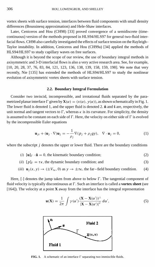
Consider two inviscid, incompressible, and irrotational fluids separated by the para-metrized planar interface0 given byX(α) = (x(α), y(α)), as shown schematically in Fig. 1.The lower fluid is denoted 1, and the upper fluid is denoted 2.n andsare, respectively, theunit normal and tangent vectors to0, whereasκ is its curvature. For simplicity, the densityis assumed to be constant on each side of0. Here, the velocity on either side of0 is evolvedby the incompressible Euler equations
u j t + (u j · ∇)u j = − 1
ρ j∇(pj + ρ j gy), ∇ · u j = 0, (1)
where the subscriptj denotes the upper or lower fluid. There are the boundary conditions
(i) [u]0 · n = 0, the kinematic boundary condition; (2)
(ii) [ p]0 = τκ, the dynamic boundary condition; and (3)
(iii ) u j (x, y)→ (±V∞, 0) asy→±∞, the far−field boundary condition. (4)
Here, [·] denotes the jump taken from above to below0. The tangential component offluid velocity is typically discontinuous at0. Such an interface is called avortex sheet(see[164]). The velocity at a pointX away from the interface has the integral representation
u(X) = 1
2π
∫γ (α′)
(X − X(α′))⊥
|X − X(α′)|2 dα′, (5)
FIG. 1. A schematic of an interface0 separating two immiscible fluids.
BOUNDARY INTEGRAL METHODS 307
whereX⊥ = (−y, x). γ is called the (unnormalized) vortex sheet strength. It gives thevelocity difference across0 by
γ = γ (α)
sα= −[u]|0 · s, (6)
wheresα =√
x2α + y2
α is the arclength metric. The velocity jump ˜γ is called the true vortexsheet strength. This representation is well known; see [14]. We will consider flows thatare 1-periodic in thex-direction. The average value, ¯γ , of γ over a period inα satisfies−γ /2= V∞.
While there is a discontinuity in the tangential component of the velocity at0, the normalcomponent,U (α), is continuous and is given by (5) as
U (α) =W(α) · n, (7)
where
W(α) = 1
2πP.V.
∫γ (α′)
(X(α)− X(α′))⊥
|X(α)− X(α′)|2 dα′ (8)
and P.V. denotes the principal value integral. This integral is called the Birkhoff–Rott inte-gral.
Using the representation (5) of the velocity, Euler’s equation at the interface, and theLaplace–Young condition, the equations of motion for the interface are
Xt = U n+ T s (9)
γt − ∂α((T −W · s) γ /sα) = −2Aρ
(sαWt · s+ 1
8∂α(γ /sα)
2− (T −W · s)Wα · s/sα)
−Fr−1yα +We−1κα. (10)
Here, the equations have been nondimensionalized on a periodicity lengthλ and the velocityscale ¯γ , and
Aρ = 1ρ
2ρis the Atwood ratio, (11)
Fr = ρ γ 2λ2
g(1ρ)λ3is the Froude number, and (12)
We= ρλ2γ 2
τλis the Weber number, (13)
where1ρ = ρ1− ρ2, and ¯ρ = (ρ1+ ρ2)/2. The Froude number measures the importanceof inertial forces relative to gravitational forces, whereas the Weber number measures theimportance of inertial forces relative to the dispersive forces of surface tension forces.
T is an (as yet) arbitrary tangential velocity that specifies the motion of the parametrizationof0. The so-calledLagrangian formulationcorresponds to choosing the tangential velocityof a point on the interface to be the arithmetic average of the tangential components of thefluid velocity on either side. That is, choosingT =W · s, in which case Eq. (10) simplifiesconsiderably.
308 HOU, LOWENGRUB, AND SHELLEY
Equation (10) is a Fredholm integral of the second kind forγt due to the presence ofγt inWt . This equation has a unique solution, and is contractive [14]. The mean ofγ is preservedby Eq. (10) and must be chosen to be−2V∞, initially, to guarantee that condition (iii ) issatisfied. Further, whileγ is evolved as an independent variable, it cannot be interpretedindependently of the parametrization. From Eq. (6), it is the ratio ˜γ = γ /sα that has aphysical interpretation, andsα is determined by the choice ofT .
Equation (9–10) realize different physical situations in different limits of the nondimen-sional parameters. For example, takingAρ = −1 gives the classical Rayleigh–Taylor prob-lem regularized by surface tension. TakingAρ = +1 gives water waves with surface tension.Taking Aρ = Fr−1 = 0 gives the Kelvin–Helmholtz problem of two density-matched, im-miscible liquids. All of these problems will be considered in the following sections.
2.3. The Sources of Stiffness and the Small-Scale Decomposition
For the Kelvin–Helmholtz problem, a natural choice of frame is the so-called“Lagrangian” frame in whichT =W · s. That is, the interface moves with the averageof the velocities on each side. The problem is then completely characterized by the WebernumberWe, and the Lagrangian formulation of the equations of motion becomes simply
Xt (α, t) = W(α, t) and (14)
γt (α, t) = We−1κα. (15)
It is this compact formulation that has been used in various studies of singularity formationin the dynamics of vortex sheets without surface tension (see, for example [42, 104, 128,131, 172]). Without surface tension, the curvature of the sheet diverges at a finite time and iscoupled to a concentration of interfacial vorticity. This is known as the “Moore” singularityafter Moore [131].
Next, we demonstrate that the Lagrangian formulation results leads to extreme differ-ential clustering of computational points during typical simulations. This results in severenumerical time step constraints when surface tension is present. This may be seen through ageneral linear analysis given by Bealeet al.[18, 19]. Linearizing around the time-dependentinertial vortex sheet0 = (x(α, t), y(α, t))with strengthγ (α, t), Bealeet al.find the leadingorder equation for thenormal componentof a perturbation at large wavenumber:
ηt t = − γ2
4s4α
ηαα + We−1
2s3α
H [ηααα] . (16)
Here,H is the Hilbert transform:
H[ f ](α) = 1
πP.V.
∫ +∞−∞
f (α′)α − α′ dα′.
Setting We−1= 0 gives the linearly ill-posed behavior of the unregularized Kelvin–Helmholtz problem. For finiteWe, this ill-posedness is regularized by a dispersion dueto caused by surface tension.
A “frozen coefficient” analysis of Eq. (16) reveals that the least restrictive time-dependentstability constraint on a stableexplicit time integration method is
1t < C We1/2 · (sαh)3/2 , wheresα = minα
sα; (17)

BOUNDARY INTEGRAL METHODS 309
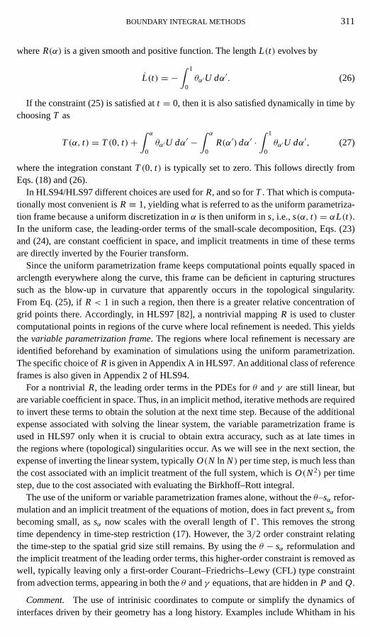
FIG. 2. The evolution of log10 (sα) for several Weber numbers.
see [18, 19] for details. Hereh = 1/N is the grid spacing, withN the number of pointsdescribing0. Since arclength spacing,1s, satisfies1s≈ sαh, Eq. (17) implies that thestability constraint is in fact determined by theminimumspacing inarclengthbetweenadjacent points on the grid.
For several “typical” simulations (same initial data, differing Weber numbers),the evo-lution of sα associated with the Lagrangian formulation is shown in Fig. 2, on a base-10logarithmic scale. Over the times shown,sα decreases in value by a factor of 104 or more.Consequently, the time-step constraint (17) decreases by at least a factor of 106, even for afixed grid sizeh. The steep drop at slightly less thant = 0.5 is the result of the compressionassociated with the shadow of the Moore singularity, which occurs attM ≈ 0.37 for thisinitial data [104]. Such strongly time-dependent time-step constraints have severely limitedprevious numerical investigations [11, 149, 151].
Once a stable spatial discretization has been obtained, the primary challenge to computingthe long time evolution of interfacial flows with surface tension lies in the construction oftime integration methods with good stability properties. It is difficult to straightforwardlyconstruct efficient implicit time integration methods as the source of the stiffness, theκα intheγ -equation, involves both a nonlinear combination of high derivatives of the interfaceposition and contributes nonlocally to the motion through theγ in the Birkhoff–Rott integral.The approach we consider to be state-of-the-art in generating such time integration methodswas first given in HLS94. It involves reformulating the equations of motion according to thefollowing three steps:(A) θ − sα formulation;(B) small-scale analysis;(C) special choicesof reference frames (tangential velocities).
(A) θ − sα formulation. Rather than usingx, y as the dynamical variables, repose theevolution in variables that are more naturally related to curvature. Motivated by the identity
310 HOU, LOWENGRUB, AND SHELLEY
θs = κ, whereθ is the tangent angle to the curve0, the evolution is formulated withθ andsα as the independent dynamical variables. The equations of motion are then given by
sαt = Tα − θαU (18)
θt = 1
sαUα + T
sαθα. (19)
γt = We−1∂α(θα/sα)+ ∂α((T −W · s) γ /sα). (20)
Givensα andθ , the position(x(α, t), y(α, t)) is reconstructed up to a translation by directintegration of
(xα, yα) = sα(cos(θ(α, t)), sin(θ(α, t))), (21)
which defines the tangent angle. The integration constant is supplied by evolving the positionat one pointX0(t).
(B) Small-scale analysis.Reformulate the equations by explicitly separating the domi-nant terms at small spatial scales. The behavior of the equations at small scales is importantbecause stability constraints (i.e., stiffness) arise from the influence of high-order termsatsmall spatial scales. In HLS94, it is shown that at small scales the Birkhoff–Rott operatorsimplifies enormously. A useful notation,f ∼ g, is introduced to mean that the differencebetweenf andg is smoother thanf andg. In HLS94, it is demonstrated that
U (α, t) ∼ 1
2sαH[γ ](α, t). (22)
That is, at small spatial scales, the normal (physical) velocity is essentially the Hilberttransform with a variable coefficient. Now, Eq. (22) allows a rewriting of the equations ofmotion in a way that separates the dominant terms at small scales. We remark that theseterms determine the stability constraints. Rewriting the equations, we obtain
θt = 1
2
1
sα
(1
sαH [γ ]
)α
+ P, (23)
γt = We−1
(θα
sα
)α
+ Q. (24)
Here,P andQ represent “lower-order” terms at small spatial scales. This is thesmall-scale decomposition. Assuming thatsα is given, the dominant small-scale terms are linearin θ andγ , but also nonlocal and variable coefficient. At this point, it is possible to applystandard implicit time integration techniques where the leading order “linear” terms arediscretized implicitly. However, we have not yet taken any advantage in choosing the tan-gential velocityT . There are choices ofT that are especially convenient in constructingefficient time integration methods and in maintaining the accuracy of the simulations.
(C) Special choices for T .Choose the tangential velocityT to preserve dynamically aspecific parametrization, up to a time-dependent scaling. In particular, require that
sα(α, t) = R(α)L(t) with∫ 1
0R(α) dα = 1, (25)
BOUNDARY INTEGRAL METHODS 311
whereR(α) is a given smooth and positive function. The lengthL(t) evolves by
L(t) = −∫ 1
0θα′U dα′. (26)
If the constraint (25) is satisfied att = 0, then it is also satisfied dynamically in time bychoosingT as
T(α, t) = T(0, t)+∫ α
0θα′U dα′ −
∫ α
0R(α′) dα′ ·
∫ 1
0θα′U dα′, (27)
where the integration constantT(0, t) is typically set to zero. This follows directly fromEqs. (18) and (26).
In HLS94/HLS97 different choices are used forR, and so forT . That which is computa-tionally most convenient isR≡ 1, yielding what is referred to as the uniform parametriza-tion frame because a uniform discretization inα is then uniform ins, i.e.,s(α, t) = αL(t).In the uniform case, the leading-order terms of the small-scale decomposition, Eqs. (23)and (24), are constant coefficient in space, and implicit treatments in time of these termsare directly inverted by the Fourier transform.
Since the uniform parametrization frame keeps computational points equally spaced inarclength everywhere along the curve, this frame can be deficient in capturing structuressuch as the blow-up in curvature that apparently occurs in the topological singularity.From Eq. (25), ifR< 1 in such a region, then there is a greater relative concentration ofgrid points there. Accordingly, in HLS97 [82], a nontrivial mappingR is used to clustercomputational points in regions of the curve where local refinement is needed. This yieldsthe variable parametrization frame. The regions where local refinement is necessary areidentified beforehand by examination of simulations using the uniform parametrization.The specific choice ofR is given in Appendix A in HLS97. An additional class of referenceframes is also given in Appendix 2 of HLS94.
For a nontrivialR, the leading order terms in the PDEs forθ andγ are still linear, butare variable coefficient in space. Thus, in an implicit method, iterative methods are requiredto invert these terms to obtain the solution at the next time step. Because of the additionalexpense associated with solving the linear system, the variable parametrization frame isused in HLS97 only when it is crucial to obtain extra accuracy, such as at late times inthe regions where (topological) singularities occur. As we will see in the next section, theexpense of inverting the linear system, typicallyO(N ln N) per time step, is much less thanthe cost associated with an implicit treatment of the full system, which isO(N2) per timestep, due to the cost associated with evaluating the Birkhoff–Rott integral.
The use of the uniform or variable parametrization frames alone, without theθ–sα refor-mulation and an implicit treatment of the equations of motion, does in fact preventsα frombecoming small, assα now scales with the overall length of0. This removes the strongtime dependency in time-step restriction (17). However, the 3/2 order constraint relatingthe time-step to the spatial grid size still remains. By using theθ − sα reformulation andthe implicit treatment of the leading order terms, this higher-order constraint is removed aswell, typically leaving only a first-order Courant–Friedrichs–Lewy (CFL) type constraintfrom advection terms, appearing in both theθ andγ equations, that are hidden inP andQ.
Comment. The use of intrinisic coordinates to compute or simplify the dynamics ofinterfaces driven by their geometry has a long history. Examples include Whitham in his
312 HOU, LOWENGRUB, AND SHELLEY
early work on shock propagation [212]; Broweret al. in work on geometrical models ofinterface evolution [29]. Strain in work on unstable solidification [181]; Schwendeman inwork on thermally driven motion of grain domain boundaries in crystallized solids [171];Goldsteinet al. in work on the elastic, overdamped dynamics of polymers [65, 71]; Houet al. in work on the inertial dynamics of filaments [80]; and Shelley and Ueda [175, 176]in work on dynamics arising in phase transitions of smectic-A materials.
(D) Extension to the general two-fluid case.When the interface0 separates two fluidswith different densities, the Atwood ratioAρ is non-zero. This means that a Fredholmintegral equation of the second kind must be solved to obtainγt due to theWt term inEq. (10). It turns out, however, that the small scale decomposition (23), (24) remains valid.This may be seen explicitly by rewriting Eq. (10) as
γt (α, t)+ K [γt ](α, t) = f (α, t), (28)
whereK is the integral operator
K [γt ](α, t) = −2Aρ
∫γt (α
′, t)[
xα(y(α, t)− y(α′, t))− yα(x(α, t)− x(α′, t))|x(α, t)− x(α′, t)|2
]dα′.
(29)
Observe that the kernel has a removable singularity atα = α′. Thus,K is smoothingat small spatial scales [81]. Further,f (α, t) in Eq. (28) contains all the terms in Eq. (10),which do not containγt . Note that of these terms,κα is still dominant at small spatial scales.Since the integral operatorI + K is invertible for|Aρ | ≤ 1 [96], we may write the solutionas
γt = f − K [(I + K )−1 f ]. (30)
Finally, sinceK is smoothing at small scales,γt ∼ f ∼ κα. This justifies the assertionabove. For additional details, refer to Appendix 1 of HLS94.
2.4. Temporal and Spatial Discretizations
Let us begin with the temporal discretizations described in HLS94/HLS97. The ODE(26) for L(t) is not stiff. Therefore it may be solved using an explicit method. For example,using the second-order Adams–Bashforth method,
Ln+1 = Ln + 1t
2
∫ 1
0
(3θnα′U
n − θn−1α′ Un−1
)dα′. (31)
ConsequentlyL is always available at the(n+ 1)st time-step. In HLS97, a fourth-ordermethod is also used to solve this ODE.
Next, consider the second-order Crank–Nicholson time discretization of Eqs. (23) and(24) in the uniform parametrization frame. The equations are discretized in Fourier space.Let θn(k) denote the Fourier transform ofθ at wavenumberk and at timetn = n1t . Let
BOUNDARY INTEGRAL METHODS 313
γ n(k) denote the analogous quantity. Then
θn+1(k)− θn−1(k)
21t= |k|
4
[(2π
Ln+1
)2
γ n+1+(
2π
Ln−1
)2
γ n−1
]+ Pn(k) (32)
γ n+1(k)− γ n−1(k)
21t= − k2
2We
[2π
Ln+1θn+1+ 2π
Ln−1θn−1
]+ Qn(k), (33)
where we have used thatH = −i sgn(k). The updatesθn+1 and γ n+1 can then be foundexplicitly by inverting a 2× 2 matrix. For details, see HLS94.
In HLS97, a 4th-order accurate, implicit, multistep method due to Ascheret al. [8] isalso used to discretize in time both the uniform and variable parametrization formulations.Using this method, Eqs. (23) and (24) may be reduced to the following single equation forθn+1,
sn+1α θn+1(α)− 1
2We
(12
25
)2
1t2
(1
sn+1α
H[θn+1
sn+1α
]α
)α
= N(α), (34)
whereN(α) is a known quantity that depends on the solutions at the previous time steps. Inthe uniform parametrization case,θn+1 is obtained explicitly by solving Eq. (34) in Fourierspace since there the equation is diagonal. In the variable parametrization case, the discretesystem is symmetric positive definite and is solved in physical space using the precon-ditioned conjugate gradient method. The application ofH is performed in Fourier space,however, so that each step of the iteration requiresO(N ln N) operations. The precondi-tioning operatorM is given by
M(θn+1) = smaxθn+1− 1
2sminWe
(12
25
)2
1t2H[θn+1α
]αα, (35)
wheresmin = minα sn+1α andsmax= maxα sn+1
α . Thus,M is constant coefficient and is di-agonalized by the Fourier transform. For details, we refer the reader to Appendix B ofHLS97.
In HLS94 and HLS97, spectrally accurate spatial discretizations are used in both theuniform and variable parametrization frames. Any differentiation, partial integration, orHilbert transform is found at the mesh points by using the discrete Fourier transform. Aspectrally accurate alternate-point discretization [172, 178] is used to compute the velocityof the interface from Eq. (8), i.e.,
ui = h
π
∑(i− j ) odd
γ j(X i − X j )
⊥
|X i − X j |2 , (36)
whereui = u(αi ) andαi = ih. The other variables in Eq. (36) are defined analogously.Finally, as noted in HLS94, time-stepping methods for vortex sheets suffer from aliasinginstabilities since they are not naturally damping at the highest modes. The instability iscontrolled by using Fourier filtering to damp the highest modes and Krasny filtering [104]to remove round-off error effects; this determines the overall accuracy of the method, andgives a formal accuracy ofO(h16). An infinite-order filter could also have been used.
314 HOU, LOWENGRUB, AND SHELLEY
Empirically, it is found that the time stepping routines discussed above remove the highorder time step constraints due to surface tension and suffer only from a first order CFL timestep restriction. In fact, the stability and convergence of these boundary integral methods hasonly recently been proved in the semidiscrete case in which time is continuous. For example,Bealeet al.(BHL96) [19] proved convergence of a class of boundary integral methods, usinga slightly different formulation (based on the velocity potential and Bernoulli’s equation)than that described previously, in the context of water waves. Ceniceros and Hou (CH98)[33] later proved convergence of a class of methods analogous to those described in thecase of interfacial flows between two liquids. An important feature of the BHL96 andCH98 stability analyses is that a certain compatibility between the choice of quadraturerule for the velocity integral (8) and the choice of spatial derivative must be satisfied onthe discrete level to achieve numerical stability. This compatibility relation is subtle andensures that a delicate balance of terms that holds on the continuous level is preserved onthe discrete level. This balance is crucial for maintaining numerical stability and is one ofthe reasons why many previous investigations suffered from numerical instability. Usinglinear stability analysis near equilibrium interfaces, BN98 [11] independently also notedand removed instability due to the incompatibility of the operators.
While the BN98 results, and the spectrally accurate method described, satisfy the compat-ibility relation, most straightforward implementations of the boundary integral equationsdo not. The compatibility condition is described most easily in the case of water waveswithout surface tension. In this case, the compatibility relation boils down to satisfying
3h( f ) j = Hh Dh( f ) j , (37)
for all discrete functionsf j , where3h is the discretization of
1
π
∫f (α)− f (α′)(α − α′)2 dα′,
which is related to the first variation of the velocity integral (8).Hh is the discretizationof the Hilbert transform using the same quadrature method as used for3h. Dh is thediscrete derivative operator. Using alternate point quadrature to evaluate the velocity, theonly compatible spatial discretization isSh, the spectral derivative with theN/2 mode setto zero. However, one may introduce appropriate Fourier filtering in the approximation ofthe velocity integral so that a version of Eq. (37) holds for all choices ofDh. Doing thisappropriately, one obtains
3h( f ρ) j = Hh Dh( f ) j , (38)
where fρ(k) = ρ(kh) f (k) andρ is defined byDh = ikρ(kh). In the case of surface tension
and two liquids, additional filtering must be used to maintain compatibility for arbitraryderivatives; alternate point quadrature and the spectral derivative are always compatible.We refer the reader to BHL96 and CH98 for further details.
2.5. The Kelvin–Helmholtz Instability, Surface Tension, and Singularities
An interface separating two immiscible fluids is susceptible to the Kelvin–Helmholtzinstability when shear develops across that interface. This is a fundamental instability of
BOUNDARY INTEGRAL METHODS 315
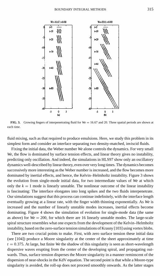
FIG. 3. Growing fingers of interpenetrating fluid forWe= 16.67 and 20. Three spatial periods are shown ateach time.
fluid mixing, such as that required to produce emulsions. Here, we study this problem in itssimplest form and consider an interface separating two density-matched, inviscid fluids.
Fixing the initial data, the Weber numberWealone controls the dynamics. For very smallWe, the flow is dominated by surface tension effects, and linear theory gives no instability,predicting only oscillation. And indeed, the simulations in HLS97 show only an oscillatorydynamics well-described by linear theory, even over very long times. The dynamics becomessuccessively more interesting as the Weber number is increased, and the flow becomes moredominated by inertial effects, and hence, the Kelvin–Helmholtz instability. Figure 3 showsthe evolution from single-mode initial data, for two intermediate values ofWeat whichonly thek = 1 mode is linearly unstable. The nonlinear outcome of the linear instabilityis fascinating: The interface elongates into long spikes and the two fluids interpenetrate.Our simulations suggest that this process can continue indefinitely, with the interface lengtheventually growing at a linear rate, with the finger width thinning exponentially. AsWeisincreased and the number of linearly unstable modes increases, inertial effects becomedominating. Figure 4 shows the simulation of evolution for single-mode data (the sameas above) forWe= 200, for which there are 16 linearly unstable modes. The large-scalespiral structure resembles what one expects from the development of the Kelvin–Helmholtzinstability, based on the zero-surface tension simulations of Krasny [103] using vortex blobs.
There are two crucial points to make. First, with zero surface tension these initial data(see [104]) produce a Moore singularity at the center of the sheet approximately at timet = 0.375. At large, but finiteWethe shadow of this singularity is seen as short-wavelengthdispersive waves erupting from the center of the developing spiral, and propagating out-wards. Thus, surface tension disperses the Moore singularity in a manner reminscent of thedispersion of near-shocks in the KdV equation. The second point is that while a Moore-typesingularity is avoided, the roll-up does not proceed smoothly onwards. As the latter stages

316 HOU, LOWENGRUB, AND SHELLEY
FIG. 4. The long-time evolution from a nearly flat sheet forWe= 200. The bottom right box shows a close-upof the thinning neck att = 1.4.
of our simulation show, the roll-up appears to be terminated by the collision of interfaceswithin the interior of the spiral, that is, the smooth dynamics is punctuated by a collision,in finite time, of the sheet with itself in the inner turns of the spiral.
As is well known, a collision of material interfaces in a flow implies the divergence ofvelocity gradients (see, e.g., HLS97). We refer to this collision as atopological singularity,since such collisions must precede a reconfiguration of fluid interfaces in a multiphaseflow (as in the pinch-off of a droplet). In HLS97, locally refined grids and high-order time-stepping are used, together with an SSD formulation, to very carefully isolate this oncomingtopological singularity, and to study its analytical structure. This study reveals the following:As the spiral forms and disparate sections of the interface come in proximity to one another,a jet begins to form and intensify, fluxing fluid into the inner core of the spiral. This jet isassociated (i) with the thin neck shown in close-up in Fig. 4f, and (ii ) with the formationof oppositely signed sheet strengths (or interfacial vorticity) on the opposing sides of thisneck. This creation of oppositely signed sheet strength is a direct consequence of surfacetension as in its absence the sheet strength is conserved in the Lagrangian frame, and ourinitial data have sheet strength of a single sign. That the thickness of this neck falls to zeroin a finite time is demonstrated in Fig. 5 (upper), which shows the neck width as a functionof time.
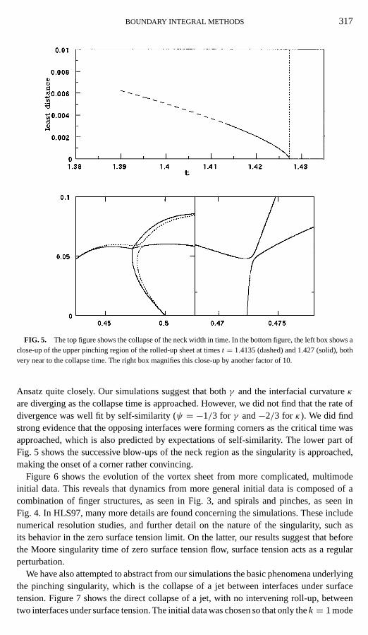
The oncoming singularity bears some signs of self-similarity. Expectations of self-similarity would suggest that
Neck Width∼ (tp − t)ψ,
wheretp is the singularity time (its estimate is shown as the vertical dashed line in Fig. 5(upper)), andψ = 2/3 the similarity exponent [95]. We find that the collapse follows this
BOUNDARY INTEGRAL METHODS 317
FIG. 5. The top figure shows the collapse of the neck width in time. In the bottom figure, the left box shows aclose-up of the upper pinching region of the rolled-up sheet at timest = 1.4135 (dashed) and 1.427 (solid), bothvery near to the collapse time. The right box magnifies this close-up by another factor of 10.
Ansatz quite closely. Our simulations suggest that bothγ and the interfacial curvatureκare diverging as the collapse time is approached. However, we did not find that the rate ofdivergence was well fit by self-similarity (ψ = −1/3 for γ and−2/3 for κ). We did findstrong evidence that the opposing interfaces were forming corners as the critical time wasapproached, which is also predicted by expectations of self-similarity. The lower part ofFig. 5 shows the successive blow-ups of the neck region as the singularity is approached,making the onset of a corner rather convincing.
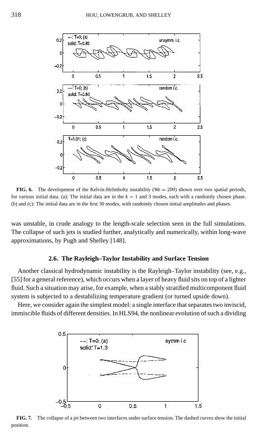
Figure 6 shows the evolution of the vortex sheet from more complicated, multimodeinitial data. This reveals that dynamics from more general initial data is composed of acombination of finger structures, as seen in Fig. 3, and spirals and pinches, as seen inFig. 4. In HLS97, many more details are found concerning the simulations. These includenumerical resolution studies, and further detail on the nature of the singularity, such asits behavior in the zero surface tension limit. On the latter, our results suggest that beforethe Moore singularity time of zero surface tension flow, surface tension acts as a regularperturbation.
We have also attempted to abstract from our simulations the basic phenomena underlyingthe pinching singularity, which is the collapse of a jet between interfaces under surfacetension. Figure 7 shows the direct collapse of a jet, with no intervening roll-up, betweentwo interfaces under surface tension. The initial data was chosen so that only thek = 1 mode
318 HOU, LOWENGRUB, AND SHELLEY
FIG. 6. The development of the Kelvin-Helmholtz instability (We= 200) shown over two spatial periods,for various initial data. (a): The initial data are in thek = 1 and 3 modes, each with a randomly chosen phase.(b) and (c): The initial data are in the first 30 modes, with randomly chosen initial amplitudes and phases.
was unstable, in crude analogy to the length-scale selection seen in the full simulations.The collapse of such jets is studied further, analytically and numerically, within long-waveapproximations, by Pugh and Shelley [148].
2.6. The Rayleigh–Taylor Instability and Surface Tension
Another classical hydrodynamic instability is the Rayleigh–Taylor instability (see, e.g.,[55] for a general reference), which occurs when a layer of heavy fluid sits on top of a lighterfluid. Such a situation may arise, for example, when a stably stratified multicomponent fluidsystem is subjected to a destabilizing temperature gradient (or turned upside down).
Here, we consider again the simplest model: a single interface that separates two inviscid,immiscible fluids of different densities. In HLS94, the nonlinear evolution of such a dividing
FIG. 7. The collapse of a jet between two interfaces under surface tension. The dashed curves show the initialposition.
BOUNDARY INTEGRAL METHODS 319
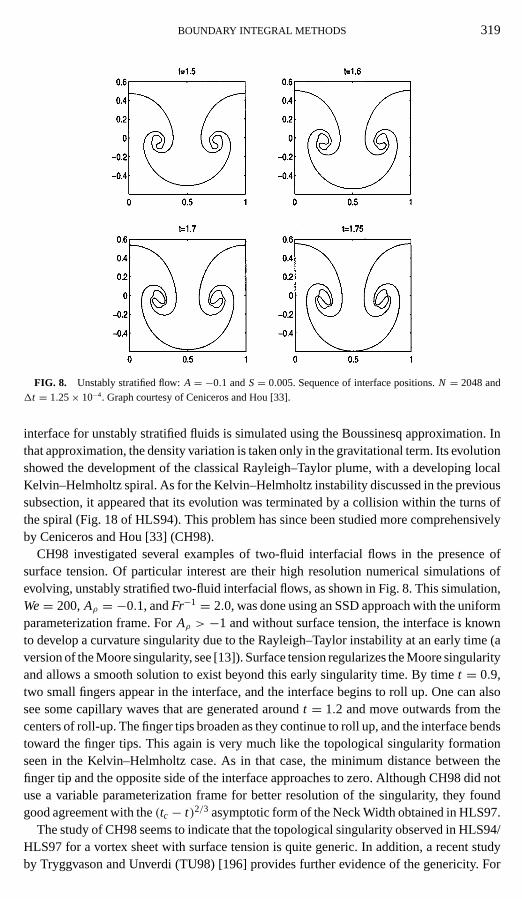
FIG. 8. Unstably stratified flow:A = −0.1 andS= 0.005. Sequence of interface positions.N = 2048 and1t = 1.25× 10⁻⁴. Graph courtesy of Ceniceros and Hou [33].
interface for unstably stratified fluids is simulated using the Boussinesq approximation. Inthat approximation, the density variation is taken only in the gravitational term. Its evolutionshowed the development of the classical Rayleigh–Taylor plume, with a developing localKelvin–Helmholtz spiral. As for the Kelvin–Helmholtz instability discussed in the previoussubsection, it appeared that its evolution was terminated by a collision within the turns ofthe spiral (Fig. 18 of HLS94). This problem has since been studied more comprehensivelyby Ceniceros and Hou [33] (CH98).
CH98 investigated several examples of two-fluid interfacial flows in the presence ofsurface tension. Of particular interest are their high resolution numerical simulations ofevolving, unstably stratified two-fluid interfacial flows, as shown in Fig. 8. This simulation,We= 200,Aρ = −0.1, andFr−1 = 2.0, was done using an SSD approach with the uniformparameterization frame. ForAρ > −1 and without surface tension, the interface is knownto develop a curvature singularity due to the Rayleigh–Taylor instability at an early time (aversion of the Moore singularity, see [13]). Surface tension regularizes the Moore singularityand allows a smooth solution to exist beyond this early singularity time. By timet = 0.9,two small fingers appear in the interface, and the interface begins to roll up. One can alsosee some capillary waves that are generated aroundt = 1.2 and move outwards from thecenters of roll-up. The finger tips broaden as they continue to roll up, and the interface bendstoward the finger tips. This again is very much like the topological singularity formationseen in the Kelvin–Helmholtz case. As in that case, the minimum distance between thefinger tip and the opposite side of the interface approaches to zero. Although CH98 did notuse a variable parameterization frame for better resolution of the singularity, they foundgood agreement with the(tc − t)2/3 asymptotic form of the Neck Width obtained in HLS97.
The study of CH98 seems to indicate that the topological singularity observed in HLS94/HLS97 for a vortex sheet with surface tension is quite generic. In addition, a recent studyby Tryggvason and Unverdi (TU98) [196] provides further evidence of the genericity. For
320 HOU, LOWENGRUB, AND SHELLEY
example, TU98 report that interfaces between two immiscible fluids, with small but finiteviscosities, exhibit structures under shear and buoyancy similar to those of their inviscidcounterparts described here and in HLS94, HLS97, and CH98.
2.7. Dynamic Generation of Capillary Waves
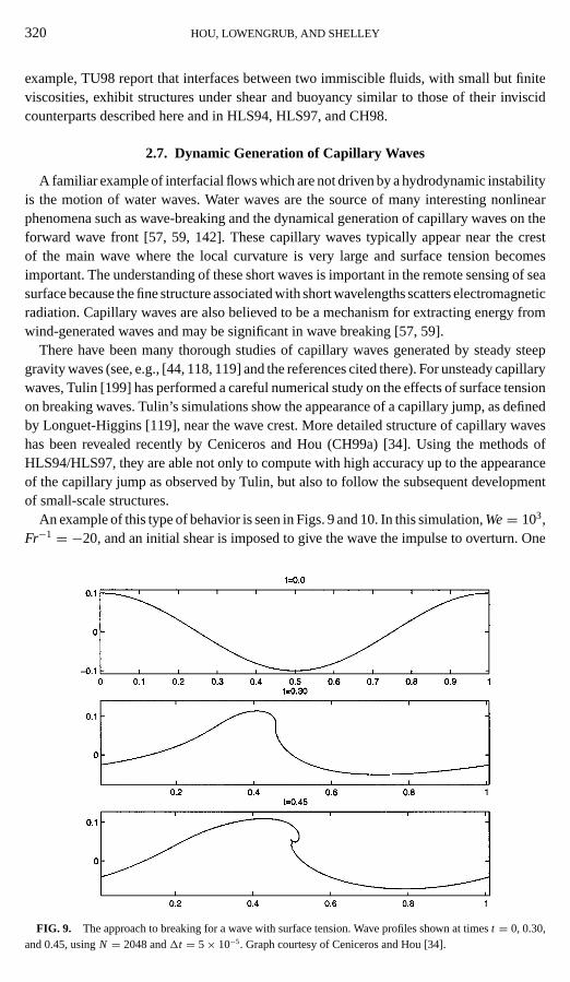
A familiar example of interfacial flows which are not driven by a hydrodynamic instabilityis the motion of water waves. Water waves are the source of many interesting nonlinearphenomena such as wave-breaking and the dynamical generation of capillary waves on theforward wave front [57, 59, 142]. These capillary waves typically appear near the crestof the main wave where the local curvature is very large and surface tension becomesimportant. The understanding of these short waves is important in the remote sensing of seasurface because the fine structure associated with short wavelengths scatters electromagneticradiation. Capillary waves are also believed to be a mechanism for extracting energy fromwind-generated waves and may be significant in wave breaking [57, 59].
There have been many thorough studies of capillary waves generated by steady steepgravity waves (see, e.g., [44, 118, 119] and the references cited there). For unsteady capillarywaves, Tulin [199] has performed a careful numerical study on the effects of surface tensionon breaking waves. Tulin’s simulations show the appearance of a capillary jump, as definedby Longuet-Higgins [119], near the wave crest. More detailed structure of capillary waveshas been revealed recently by Ceniceros and Hou (CH99a) [34]. Using the methods ofHLS94/HLS97, they are able not only to compute with high accuracy up to the appearanceof the capillary jump as observed by Tulin, but also to follow the subsequent developmentof small-scale structures.
An example of this type of behavior is seen in Figs. 9 and 10. In this simulation,We= 103,Fr−1 = −20, and an initial shear is imposed to give the wave the impulse to overturn. One
FIG. 9. The approach to breaking for a wave with surface tension. Wave profiles shown at timest = 0, 0.30,and 0.45, usingN = 2048 and1t = 5× 10⁻⁵. Graph courtesy of Ceniceros and Hou [34].
BOUNDARY INTEGRAL METHODS 321
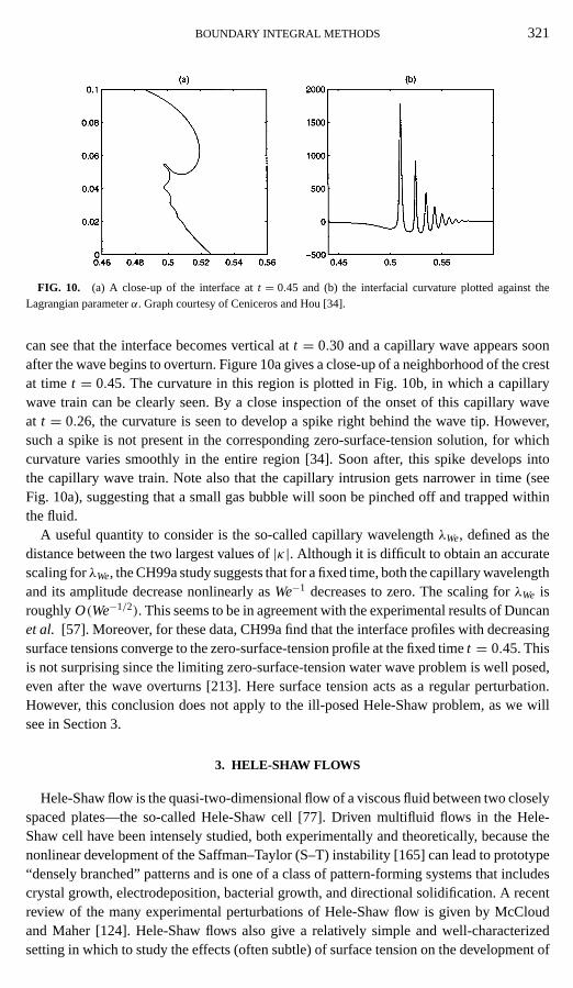
FIG. 10. (a) A close-up of the interface att = 0.45 and (b) the interfacial curvature plotted against theLagrangian parameterα. Graph courtesy of Ceniceros and Hou [34].
can see that the interface becomes vertical att = 0.30 and a capillary wave appears soonafter the wave begins to overturn. Figure 10a gives a close-up of a neighborhood of the crestat time t = 0.45. The curvature in this region is plotted in Fig. 10b, in which a capillarywave train can be clearly seen. By a close inspection of the onset of this capillary waveat t = 0.26, the curvature is seen to develop a spike right behind the wave tip. However,such a spike is not present in the corresponding zero-surface-tension solution, for whichcurvature varies smoothly in the entire region [34]. Soon after, this spike develops intothe capillary wave train. Note also that the capillary intrusion gets narrower in time (seeFig. 10a), suggesting that a small gas bubble will soon be pinched off and trapped withinthe fluid.
A useful quantity to consider is the so-called capillary wavelengthλWe, defined as thedistance between the two largest values of|κ|. Although it is difficult to obtain an accuratescaling forλWe, the CH99a study suggests that for a fixed time, both the capillary wavelengthand its amplitude decrease nonlinearly asWe−1 decreases to zero. The scaling forλWe isroughlyO(We−1/2). This seems to be in agreement with the experimental results of Duncanet al. [57]. Moreover, for these data, CH99a find that the interface profiles with decreasingsurface tensions converge to the zero-surface-tension profile at the fixed timet = 0.45. Thisis not surprising since the limiting zero-surface-tension water wave problem is well posed,even after the wave overturns [213]. Here surface tension acts as a regular perturbation.However, this conclusion does not apply to the ill-posed Hele-Shaw problem, as we willsee in Section 3.
3. HELE-SHAW FLOWS
Hele-Shaw flow is the quasi-two-dimensional flow of a viscous fluid between two closelyspaced plates—the so-called Hele-Shaw cell [77]. Driven multifluid flows in the Hele-Shaw cell have been intensely studied, both experimentally and theoretically, because thenonlinear development of the Saffman–Taylor (S–T) instability [165] can lead to prototype“densely branched” patterns and is one of a class of pattern-forming systems that includescrystal growth, electrodeposition, bacterial growth, and directional solidification. A recentreview of the many experimental perturbations of Hele-Shaw flow is given by McCloudand Maher [124]. Hele-Shaw flows also give a relatively simple and well-characterizedsetting in which to study the effects (often subtle) of surface tension on the development of
322 HOU, LOWENGRUB, AND SHELLEY
singularities, on pattern selection, and as a physical regularization of an ill-posed system.(Like the Kelvin–Helmholtz system, Hele-Shaw flows can have linear growth rates that scalelinearly with wavenumber.) A much better theoretical understanding of these problems hasfollowed from analysis, guided or validated by highly accurate and efficient simulations. Arecent review of the role of surface tension in Hele-Shaw flows is given by Tanveer [185]. Acomprehensive bibliography on Hele-Shaw and Stokes flows has been compiled by Gillowand Howison [63].
The usual starting point for theoretical investigations of Hele-Shaw flows is Darcy’s law.Consider two incompressible, viscous, and immiscible fluids in a Hele-Shaw cell, separatedby a planar interface0. As before, letj = 1 or 2 label the two fluids. In a Hele-Shaw cell,the (gap-averaged) velocity of each fluid (j ) is given by Darcy’s law, together with theincompressibility constraint
u j (x, y) = − b2
12µ j(∇ pj (x, y)− ρ j F(x, y)), ∇ · u j = 0, (39)
whereb is the cell gap width,µ j the fluid viscosity,ρ j its density, andF = −∇8 isa body force (usually divergence-free, e.g., gravitational). Boundary conditions typicallyused are the kinematic and dynamic boundary conditions as given in Eqs. (2) and (3).These are augmented by far-field boundary conditions on the velocity or pressure. Takingthe divergence of Eq. (39) shows thatp is harmonic, which is the basis from which mostnumerical treatments proceed.
3.1. Historical Perspective
Many different numerical approaches have been applied to simulating Hele-Shaw flows.These include volume-of-fluid methods (e.g., [100, 210]), boundary element methods (e.g.,[75]), level set and immersed boundary methods [86], and statistical methods based ondiffusion-limited aggregation (e.g., [7, 116]). Methods based on conformal mapping havelong been used to study dynamics of Hele-Shaw flows (see [23, 45, 185] for reviews andreferences). However, conformal mapping methods apply most naturally to singly connecteddomains, and can have difficulties with efficiently including the effect of surface tension.As a numerical method, the most sophisticated version of conformal mapping seems thatdue to Bakeret al. [12], who solve a well-posed evolution problem for zero surface tensionby analytically continuing initial data and equations of motion into the complex plane, andexplicitly tracking the solution’s poles and other singularities.
Due to their natural applicability, flexibility, and potential for high accuracy, boundaryintegral methods have developed into a powerful method for simulating Hele-Shaw flows.Their first application to study dynamics seems to be due to Tryggvason and Aref [194,195], who in a highly ambitious work studied two-fluid mixing via a Rayleigh–Taylor in-stability and the interaction of S–T fingers. Posing the interfacial velocity in terms of avortex sheet, they gave an integral equation of the 2nd kind for its strengthγ , essentiallyof the form in Eq. (28) (which is forγt ). The integral equation was solved via iteration(similarly to [14] for inviscid waves), coupled to a vortex-in-cell (VIC) approach for therapid evaluation of the Birkhoff–Rott integral. In studying mixing, they were able to achieveconsiderable ramification of the interface, though this was likely aided by the smoothingof VIC methods. This work was soon followed by Davidson [47, 48] and DeGregoriaand Schwartz [50–52]. Davidson [47] posed a boundary integral representation, and used it

BOUNDARY INTEGRAL METHODS 323
subsequently [48] to study the development of S–T fingers to modest amplitude. DeGregoriaand Schwartz studied various aspects of tip-splitting and the stability of S–T fingers. Theirboundary integral approach was coupled to a grid redistribution strategy that kept com-putational points in regions of high curvature, and used a a stiff ODE solver to reducethe stiffness from surface tension. Meiburg and Homsy [127] employed a vortex sheet de-scription, with the interface discretized as circular arcs, to study aspects of splitting andfinger instability. Following Daiet al. [45], who used conformal mapping methods, Daiand Shelley [46] applied boundary integral methods (discretized to infinite order) to studyregularization of Hele-Shaw flows by surface tension, and also the interaction of surfacetension and noise. They partially ameliorated the stiffness of surface tension by choos-ing a dynamical frame that kept computational points almost uniformly spaced. They alsoapplied Krasny filtering [104], to control growth of round-off errors in their simulations.Using a vortex sheet representation, Whitaker [211] compared the effect of different spatialdiscretizations on simulating propagating fingers. Power [144] used a boundary integral rep-resentation to simulate the initial development of the S–T instability for two fluids in a radialgeometry.
3.2. The Small-Scale Decomposition for Hele-Shaw Flows
In HLS94 [81], we developed the SSD for Hele-Shaw flows (described below). Thisefficiently subverted the stiffness due to surface tension, and as with inertial vortex sheets,has allowed the accurate and long-time simulation of many prototypical Hele-Shaw flows.Further, given the close analogy of Hele-Shaw flow to solidification models in materialsscience, much of the numerical technique is immediately applicable there (see next section).
That the velocity field has the form given in Eq. (5) follows from Darcy’s law (39)(which implies that the velocityu j is irrotational), the incompressibility constraint, andthe kinematic and dynamic boundary conditions. An equation forγ follows from these,together with the Laplace–Young condition; see [194] or [46] for details. In nondimensionalvariables,γ satisfies
γ = −2AµsαW · s+ Sκα + RF · s. (40)
Here,Aµ = (µ1− µ2)/(µ1+ µ2) is the Atwood ratio of the viscosities,S is a nondimen-sional surface tension, andR is a signed measure of density stratification (ρ1 < ρ2 impliesR< 0). Due to the presence ofγ in the velocityW, Eq. (40) is a Fredholm integral equationof the second kind forγ , and is, in general, uniquely solvable (see [14]).
For Hele-Shaw flows, the effect of surface tension is dissipative at small scales and givesa higher order time-step constraint than for inertial flows. Again using a “frozen coefficient”analysis of the equations of motion, Bealeet al. [21] showed that least restrictive stabilitytime-step bound on an explicit integration scheme was the time-dependent constraint
1t < C · (sαh)3/S, (41)
wheresα = minα sα. This is a much stricter constraint than that for the inertial case (Eq. (39)).Again, the stability constraint is determined by the minimum grid spacing in arclength—perhaps strongly and adversely time-dependent—but the bound in terms ofsα is also quadrat-ically smaller. The lack of robust and efficient methods for subverting such constraints hasseverely limited simulations of Hele-Shaw and related flows.
324 HOU, LOWENGRUB, AND SHELLEY
For the Hele-Shaw case, in HLS94 the small-scale analysis shows that the equations ofmotion can be given in the form
θt = S
2
1
sα
(1
sαH[θα
sα
]α
)α
+ N(α, t), (42)
where, as in Eq. (23), the term dominant at small length-scales is separated out, andN isthe remaining, lower-order, terms.
The majority of simulations of Hele-Shaw flow have usedR≡ 1, which removes thevariable coefficient nature of Eq. (42). Thus, Eq. (42) simplifies to
θt = S
2
(2π
L
)3
H[θααα] + N(α). (43)
Equation (43) is posed together with Eq. (26), the ODE for evolvingL, and is a completespecification of the interfacial problem, with the highest order, linear behavior prominentlydisplayed. This term is now diagonalizable by the Fourier transform, and so
θ t (k) = −S
2
(2π
L
)3
|k|3θ (k)+ N(k). (44)
Implicit time integration methods can now be easily applied. As an example, considerlinear propagator methods, which factor out the leading order linear term prior to dis-cretization. They usually provide stable, even high-order, methods for integrating diffusiveproblems. The first use of such a method (of which the authors are aware) was by Rogallo[157] in simulations of the Navier–Stokes equations, though it has been rediscovered andused by several researchers in different contexts. For Hele-Shaw, Eq. (44) is rewritten as
∂
∂tψ(k, t) = exp
(S
2(2π |k|)3
∫ t
0
dt′
L3(t ′)
)N(k, t), (45)
where
ψ(k, t) = exp
(S
2(2π |k|)3
∫ t
0
dt′
L3(t ′)
)θ (k, t). (46)
Equation (45) follows from Eq. (44) by finding an integrating factor to incorporate the linearterm into the time derivative. It is now Eq. (45) that is discretized using the second-orderAdams–Bashforth method. In terms ofθ , the result is
θn+1(k) = ek(tn, tn+1)θn(k)+ 1t
2(3ek(tn, tn+1)N
n(k)− ek(tn−1, tn+1)Nn−1(k)), (47)
wheretn = n1t , and
ek(t1, t2) = exp
(−S
2(2π |k|)3
∫ t2
t1
dt′
L3(t ′)
). (48)
The use of “linear propagator” is now clear;θ at thenth time-step is propagated forwardto the(n+ 1)st time-step at the exact exponential rate associated with the linear term. IfN ≡ 0, this yields theexactsolution to the linear problem. Of course, the factore(t1, t2)still has a continuous time dependence through the presence of integrals. These integralsare evaluated by evolving auxiliary ODEs for the integrand, and forL(t). Clearly, linearpropagator methods can be formulated with high-order methods.

BOUNDARY INTEGRAL METHODS 325
FIG. 11. The evolution of an expanding gas bubble in a Hele-Shaw cell.
3.3. Pattern Formation
Hele-Shaw flows can give rise to the formation of beautiful patterns—this is one aspectof the physicist’s and mathematician’s interest in them. In this section, we briefly discussseveral scenarios and simulations of pattern formation.
From HLS94, Fig. 11 shows the simulation of a gas bubble expanding outwards into aHele-Shaw fluid (see [45, 46]) over long times. From the competition of surface tensionwith the fluid pumping, this simulation shows the development of ramification throughsuccessive tip-splitting events—the S–T instability—and the competition between adjacentfingers. This simulation is also spectrally accurate (infinite order) in space, and uses a second-order in time linear propagator method to integrate the small-scale decomposition. Thereare no high-order time-step constraints. The fluid velocity is evaluated from the discretizedBirkhoff–Rott integral inO(N) operations using the Fast Multipole Method of Greengardand Rokhlin [74]. The integral equation forγ (arising from the viscosity contrast) is solvedvia the iterative linear system solver GMRES, using an SSD-based preconditioner [163, 72].The operation count isO(N) at each time-step, whereN is the number of points describingthe boundary. HereN = 4096 and1t = 0.001. This time step is 103 times larger than thatused by Dai and Shelley [46] in computations of a similar flow using an explicit methodwith a lesser number of points, and the interface here has developed far more structure.
A very different manifestation of the S–T instability and pattern formation is seen inFig. 12. This simulation, due to Shelleyet al. (see [174]) and using SSD-based methods,shows the atypical patterns that can form at the liquid/gas interface that bounds a blob ofviscous fluid, as the upper plate of a Hele-Shaw cell is lifted. This lifting puts the fluid blobunder a lateral straining flow, sucking in the interface and causing it to buckle. This basicmechanism, though coupled to a much different material rheology, is likely responsible forproducing the permanent patterns left behind after some adhesive tapes are pulled up. Theresulting short-lived patterns can resemble a network of connections with triple junctions.A likewise odd pattern formation is seen in Fig. 13, from Lowengrub and Shelley (1999,unpublished), which shows the nonlinear development of the S–T instability on a liquidbubble in a spinning Hele-Shaw cell (see [32] for related experiments). Here the central

326 HOU, LOWENGRUB, AND SHELLEY
FIG. 12. The evolution of a contracting fluid blob as the cell gap-width is increased in time. Graph courtesyof Shelleyet al. [174].
bubble throws out attached droplets of fluid, which then themselves become susceptible tothe S–T instability, throwing out fingers which will perhaps themselves form new droplets.Such flows are relevant to the manufacturing process of spin coating, where it is of interestto control such instabilities.
In a set of beautiful simulations that sought to establish a concrete connection betweenHele-Shaw flows and dendritic solidification, Almgrenet al.[4] (ADH) used an SSD formu-lation to compute the long-time growth of “dendrites” in a Hele-Shaw flow with anisotropicsurface tension. Figure 14 shows a sample simulation from this work. As in the simulationfrom HLS94 described above, this shows an expanding gas bubble, but with the pressure
FIG. 13. The centrifugal instability of a liquid bubble in a rotating Hele-Shaw cell. Graph courtesy ofLowengrub and Shelley (unpublished).
BOUNDARY INTEGRAL METHODS 327
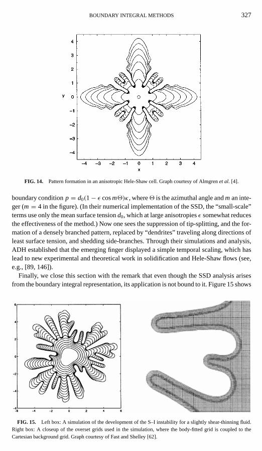
FIG. 14. Pattern formation in an anisotropic Hele-Shaw cell. Graph courtesy of Almgrenet al. [4].
boundary conditionp = d0(1− ε cosm2)κ, where2 is the azimuthal angle andman inte-ger (m= 4 in the figure). (In their numerical implementation of the SSD, the “small-scale”terms use only the mean surface tensiond0, which at large anisotropiesε somewhat reducesthe effectiveness of the method.) Now one sees the suppression of tip-splitting, and the for-mation of a densely branched pattern, replaced by “dendrites” traveling along directions ofleast surface tension, and shedding side-branches. Through their simulations and analysis,ADH established that the emerging finger displayed a simple temporal scaling, which haslead to new experimental and theoretical work in solidification and Hele-Shaw flows (see,e.g., [89, 146]).
Finally, we close this section with the remark that even though the SSD analysis arisesfrom the boundary integral representation, its application is not bound to it. Figure 15 shows
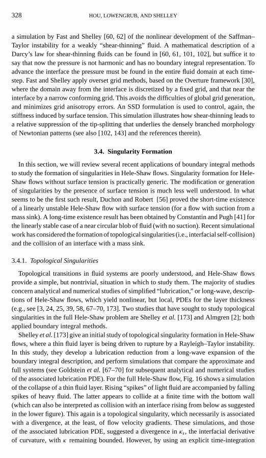
FIG. 15. Left box: A simulation of the development of the S–I instability for a slightly shear-thinning fluid.Right box: A closeup of the overset grids used in the simulation, where the body-fitted grid is coupled to theCartesian background grid. Graph courtesy of Fast and Shelley [62].
328 HOU, LOWENGRUB, AND SHELLEY
a simulation by Fast and Shelley [60, 62] of the nonlinear development of the Saffman–Taylor instability for a weakly “shear-thinning” fluid. A mathematical description of aDarcy’s law for shear-thinning fluids can be found in [60, 61, 101, 102], but suffice it tosay that now the pressure is not harmonic and has no boundary integral representation. Toadvance the interface the pressure must be found in the entire fluid domain at each time-step. Fast and Shelley apply overset grid methods, based on the Overture framework [30],where the domain away from the interface is discretized by a fixed grid, and that near theinterface by a narrow conforming grid. This avoids the difficulties of global grid generation,and minimizes grid anisotropy errors. An SSD formulation is used to control, again, thestiffness induced by surface tension. This simulation illustrates how shear-thinning leads toa relative suppression of the tip-splitting that underlies the densely branched morphologyof Newtonian patterns (see also [102, 143] and the references therein).
3.4. Singularity Formation
In this section, we will review several recent applications of boundary integral methodsto study the formation of singularities in Hele-Shaw flows. Singularity formation for Hele-Shaw flows without surface tension is practically generic. The modification or generationof singularities by the presence of surface tension is much less well understood. In whatseems to be the first such result, Duchon and Robert [56] proved the short-time existenceof a linearly unstable Hele-Shaw flow with surface tension (for a flow with suction from amass sink). A long-time existence result has been obtained by Constantin and Pugh [41] forthe linearly stable case of a near circular blob of fluid (with no suction). Recent simulationalwork has considered the formation of topological singularities (i.e., interfacial self-collision)and the collision of an interface with a mass sink.
3.4.1. Topological Singularities
Topological transitions in fluid systems are poorly understood, and Hele-Shaw flowsprovide a simple, but nontrivial, situation in which to study them. The majority of studiesconcern analytical and numerical studies of simplified “lubrication,” or long-wave, descrip-tions of Hele-Shaw flows, which yield nonlinear, but local, PDEs for the layer thickness(e.g., see [3, 24, 25, 39, 58, 67–70, 173]. Two studies that have sought to study topologicalsingularities in the full Hele-Shaw problem are Shelleyet al. [173] and Almgren [2]; bothapplied boundary integral methods.
Shelleyet al.[173] give an initial study of topological singularity formation in Hele-Shawflows, where a thin fluid layer is being driven to rupture by a Rayleigh–Taylor instability.In this study, they develop a lubrication reduction from a long-wave expansion of theboundary integral description, and perform simulations that compare the approximate andfull systems (see Goldsteinet al. [67–70] for subsequent analytical and numerical studiesof the associated lubrication PDE). For the full Hele-Shaw flow, Fig. 16 shows a simulationof the collapse of a thin fluid layer. Rising “spikes” of light fluid are accompanied by fallingspikes of heavy fluid. The latter appears to collide at a finite time with the bottom wall(which can also be interpreted as collision with an interface rising from below as suggestedin the lower figure). This again is a topological singularity, which necessarily is associatedwith a divergence, at the least, of flow velocity gradients. These simulations, and thoseof the associated lubrication PDE, suggested a divergence inκs, the interfacial derivativeof curvature, withκ remaining bounded. However, by using an explicit time-integration

BOUNDARY INTEGRAL METHODS 329
FIG. 16. The collapse of a thin fluid layer, under an unstable density stratification, in the Hele-Shaw cell. Thelower graph shows the “final” interface in a commonx − y scale. Courtesy of Shelleyet al. [66].
scheme these simulations employ only 129 spatial points because of the stiffness fromsurface tension. And so, while the spatial accuracy was of infinite order, the resolutionwas far short of that necessary to capture reliably the details of the singularity. It was thissimulation that originally motivated the development of the small-scale decomposition.
As said above, Constantin and Pugh [41] have proven the long-time existence of smoothsolutions for the Hele-Shaw flow of a blob of fluid initially close to being circular. Theyalso show that a circular blob is asymptotically stable, with these solutions relaxing to it.Almgren [2] has given strong numerical evidence that their result does not hold far fromequilibrium. He considered the evolution of singly connected blobs that initially had adumbbell shape, with a thin flat neck of fluid connecting the two halves. His conjecture wasthat in the process of the domain seeking to minimize its interfacial length—this is a curve-shortening dynamics—the neck could collapse in width, forming a flow singularity. Unlikethe problem considered above, this flow is “unforced” as there is no source of instability,such as a density stratification or mass source, and is driven purely by the surface tensionat the boundary. To study this numerically, Almgren employs an SSD formulation, with avariable parameterization frame (Eq. (25)) that clusters computational points in the neckregion. Rapid evaluation of the spatial interactions is done via the Fast Multipole Method[74], with GMRES [163] used to solve the integral equation for the vortex sheet strength. Hissimulations appear to confirm his conjecture, with the apparent singularity similar to thatsuggested above by the simulations of Shelleyet al., and in agreement with the predictionsof lubrication theory.
3.4.2. Hele-Shaw Flow with Suction
Consider a blob of fluid in a Hele-Shaw cell that contains a point mass sink that removesfluid at a constant rate. In this case, all of the fluid will be removed within a finite time,giving an upper bound on the time of existence of the flow. The question is: Does anythinginteresting happen beforehand? For example, might the bounding interface collide with the
330 HOU, LOWENGRUB, AND SHELLEY
mass sink first, giving a singularity? For zero surface tension it has been shown that priorto the fluid being completely removed, the bounding interface can form cusps, or collidewith itself, or reach the sink, and that only a circular blob with the sink at its center doesnot develop singularities [79]. For nonzero surface tension, Howisonet al.have attempted aperturbation analysis of such a flow, using knowledge of the zero-surface-tension solutions[87]. Assuming that surface tension is only important where curvature is large, they posit theexistence of a self-similar steady-state solution (where on an inner scale surface tension isrescaled to be order one). Their analysis predicts that small surface tension could cause theinterface in the neighborhood of the cusp to propagate rapidly as a narrow jet, analogous toa thin crack. However, the existence of such a self-similar steady-state solution is unknown,and the effects of very small surface tension past the cusp singularity time remained unclear.For nonzero surface tension, Tian [192] has shown that a singularity must occur if the masssink and center of mass of the fluid domain do not coincide. The form of this singularity isnot identified through his analysis.
Kelly and Hinch [97] studied numerically the effects of surface tension on a Hele-Shawflow with suction. Using a boundary integral method ([98]; second order in space and time,with explicit time-stepping) they showed that the cusp of the zero surface tension solutionswas avoided. However, their simulations are limited by modest spatial resolution (200 gridpoints).
Nie and Tian [137] have performed a more resolved numerical study of the interfacedynamics of a Hele-Shaw flow with suction. To reach high spatial resolutions (up to4096 points) and accuracy, they use a spectrally accurate SSD formulation, with a Crank–Nicholson time discretization. Beginning with data that for zero surface tension would forma finite-time cusp (away from the sink), they find that surface tension induces a collision ofthe interface with the sink, with the interface forming a corner at the instant of impact. Theyalso provide a resolution study of their simulations in the neighborhood of the singularityand suggest that the sink is approached by the interface as a square root in time.
Ceniceroset al. [36] (CHS) have provided a subsequent, yet more comprehensive study,considering both the asymptotic behavior as surface tension tends to zero, and the effect ofhaving an external fluid—the so-called Muskat problem. Their numerical approach is alsobased on the SSD formulation coupled to 4th-order implicit and stable integration scheme[8]. Because of the ill-posedness of the zero surface tension limit, they control the spuriousgrowth of round-off errors using Krasny filtering [104]. They also successively double thenumber of points, up to 16,384, whenever the Nyquist frequency begins to rise above thefilter level (usually 10−12).
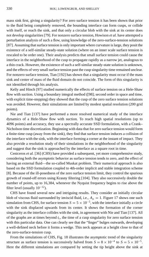
CHS have found several new and intriguing results. They consider an initially circularblob of viscous fluid surrounded by inviscid fluid, i.e.,Aµ = 1. Figure 17 shows one suchsimulation from CHS, for surface tensionS= 5× 10⁻⁵, with the interface initially a circlewith the sink displaced upwards from its center. It shows the formation of the cornersingularity as the interface collides with the sink, in agreement with Nie and Tian [137]. Allof the graphs are at times beyondtc, the time of a cusp singularity for zero surface tensionwith this particular data. One can clearly see that the “finger” bulges outwards, developinga well-defined neck before it forms a wedge. This neck appears at a height close to that ofthe zero-surface-tension cusp.
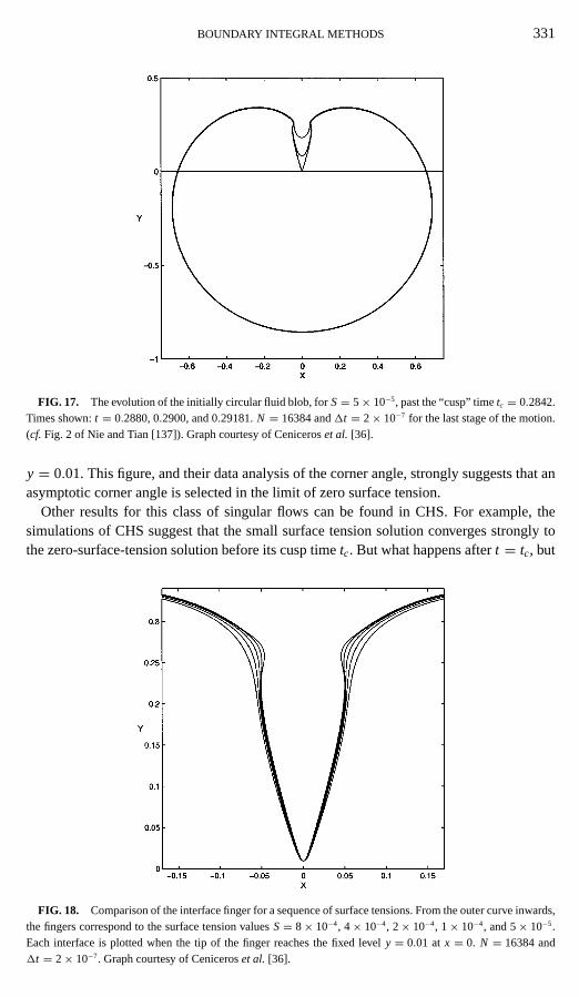
From the simulations of CHS, Fig. 18 illustrates the asymptotic trend of the singularitystructure as surface tension is successively halved fromS= 8× 10⁻⁴ to S= 5× 10⁻⁵.Here the different simulations are compared by setting the tip height above the sink at
BOUNDARY INTEGRAL METHODS 331
FIG. 17. The evolution of the initially circular fluid blob, forS= 5× 10⁻⁵, past the “cusp” timetc = 0.2842.Times shown:t = 0.2880, 0.2900, and 0.29181.N = 16384 and1t = 2× 10⁻⁷ for the last stage of the motion.(cf. Fig. 2 of Nie and Tian [137]). Graph courtesy of Ceniceroset al. [36].
y = 0.01. This figure, and their data analysis of the corner angle, strongly suggests that anasymptotic corner angle is selected in the limit of zero surface tension.
Other results for this class of singular flows can be found in CHS. For example, thesimulations of CHS suggest that the small surface tension solution converges strongly tothe zero-surface-tension solution before its cusp timetc. But what happens aftert = tc, but
FIG. 18. Comparison of the interface finger for a sequence of surface tensions. From the outer curve inwards,the fingers correspond to the surface tension valuesS= 8× 10⁻⁴, 4× 10⁻⁴, 2× 10⁻⁴, 1× 10⁻⁴, and 5× 10⁻⁵.Each interface is plotted when the tip of the finger reaches the fixed levely = 0.01 atx = 0. N = 16384 and1t = 2× 10⁻⁷. Graph courtesy of Ceniceroset al. [36].

332 HOU, LOWENGRUB, AND SHELLEY
before the interface reaches the sink? Their simulations suggest that the limiting finger hasa rounded end (it hasn’t yet reached the sink), but with a neck formed by two indentedcorners. The beginning of these limiting corners can be seen in Fig. 18. These results seemat odds with the predictions of the crack model of Howisonet al.[87], and further details ofthis comparison are found in CHS [36]. CHS also study the two-phase Hele-Shaw problem(Aµ < 1), finding that larger viscosity in the exterior fluid prevents the formation of the neck,leads to the development of thinner fingers, and that the asymptotic wedge angle apparentlydecreases towards zero (becoming cusp-like) as the viscosities approach equality (Aµ = 0).
It is natural to ask how the behavior of the interface would be in the corresponding 3-DDarcy flow. This has been studied recently by Ceniceros and Si [37], who find the situationvery similar to that of 2-D Hele-Shaw flow (surprisingly, the azimuthal component ofsurface tension did not appear to play a dominant role, and no “pinching” singularities wereobserved).
3.5. Finger Selection and Noise Effects in Hele-Shaw Cells
As illustrated above, morphological instabilities are common to pattern formation prob-lems. The non-equilibrium growth of crystals and directional solidification are some ofthe best known examples. Due to the underlying Mullins–Sekerka instability, the system isvery sensitive to small perturbations and can originate convoluted interfacial patterns. Thegeneric mechanisms in the formation of these complex patterns are present in the simplerproblem of Hele-Shaw, and a fundamental question is what is the role of surface tension inthe formation of these patterns. It can be surprisingly subtle.
In the absence of surface tension, many exact analytic solutions are known for Hele-Shawflows. It is natural to use the knowledge of these exact solutions to perform a perturbationanalysis around these solutions. Intuitively, one might think that so long as the zero surfacetension solution existed and was smooth, the small-surface-tension solution would convergeto it in the limit of zero surface tension. However, this intuition must confront the fact thatthe zero surface flows can be ill-posed (or rather, well-posed only for analytic initial data inthe space of appropriate analytic norms), and that small perturbations will generically leadto singularity.
These considerations lead Dai and Shelley [46] to numerically study whether surfacetension acted as regular perturbation to a smooth, but unstable, zero surface tension flow(see also [45]). They investigated the influence of precision and its associated round-offerrors—computing in up to 30 digits of precision—and separated those flow structures thatseemed intrinsic to surface tension from those induced through the growth of round-offerrors (see also [4] on the question of side-branching). For their initial data, they concludedthat surface tension was indeed acting as a regular perturbation.
However, the asymptotic theory of Tanveer [184, 185] and Siegelet al.[179] suggests thatsmall surface tension could be a singular perturbation for certain other initial data, even ifthe limiting zero-surface-tension solution were perfectly smooth. The reason is that surfacetension, through the curvature, can introduce a new analytic structure (the so-called daughtersingularity) att = 0+which could subsequently impinge upon the physical domain by a timefinite and independent of the surface tension. That is, for such initial data the limiting solutionafter a finite time would not be the zero surface tension solution. If true, this is a profoundresult both for the mathematical understanding of surface tension and its effects, and for themore general study of regularizations of ill-posed systems or systems yielding singularity.

BOUNDARY INTEGRAL METHODS 333
In their simulational studies, Siegelet al. have given strong evidence supporting theseanalytical predictions. In part, these studies were done using a boundary integral method,with an SSD formulation for the dynamics [81], as well as conformal mapping methods asin Dai and Shelley [46], to achieve high resolution for the interfacial flow. Unfortunately,because of the extreme sensitivity of the evolution to round-off errors, Siegelet al. findit very difficult to compute for very small surface tensions (S< 10−5), even if quadrupleprecision (30 digits) is used.
For this class of initial data, Ceniceros and Hou [35] (CH99b) have developed a sophis-ticated numerical approach to investigate the limiting behavior for small surface tension.Their method relies on three observations. The first is that noise can be significantly reducedby a parameterization that yields a compact representation of the solution in Fourier space.Out of the many choices (Lagrangian, equal-arclength, etc.), it is the conformal mappingrepresentation that gives the most compact parameterization of the interface. This compactparameterization was used likewise by Dai and Shelley [46] and by Siegelet al. [179] intheir previous studies. An advantage of using the conformal map formulation [40] is that theevaluation of the velocity integral can be done via Fast Fourier Transform inO(N log(N))operations. Further, it allows Krasny filtering [104] to be used very effectively to separatenoise from the physical solution for the majority of high to intermediate modes.
The second observation is that the daughter singularity, born att = 0+, is of amplitudeO(S · t) for small times. Therefore, initially it requires many digits to capture the spectralproperty of this complex singularity in the physical domain. To alleviate this difficulty, theyderive a scaled equation wherein the amplitude of the daughter singularity isO(1) and canthen be captured more effectively.
The third observation is that one needs to perform a resolution study in the precisionand filter level, and to compute in very high precision for small surface tension (see alsoDai and Shelley [46], and Shelley [172] for related studies). At small surface tensions, veryhigh precision arithmeticis used to solve numerically the scaled equation (up to 80 digits,using the multiprecision package of Bailey [9]). High precision has the additional benefitof reducing the amplitude of round-off error.
Each of these ingredients is essential to simulating the dynamics accurately at the verysmall surface tensions considered in CH99b (four orders of magnitude smaller than thoseused by Siegelet al.). Consequently, CH99b have provided much stronger support forsurface tension being a singular perturbation to Hele-Shaw flow. We summarize now thenumerical study of CH99b. Following Siegelet al. [179], they choose as initial data anexpanding bubble with three-fold symmetry (see Fig. 11 of [179]), for which the zero-surface-tension solution forms three cusp singularities attc = 0.3301. According to theasymptotic theory [179, 184], surface tension should produce anO(1) perturbation fromthe zero-surface-tension solution around the much earlier timetd = 0.0463—the daughtersingularity impact time, found by solving an ODE [184]—no matter how small the surfacetension, and even though the zero-surface-tension solution is still smooth att = td.
Figures 19 and 20 show some of the results from their study. ForS= 10−8, Fig. 19shows the evolution of the interfacial curvature, in the “tip” region (where the cusp wouldform for S= 0), at times neartd. Here the effect of the daughter singularity on the physicaldomain can be seen. Att = 0.043, the tip curvature flattens in a very localized finite region,and fromt = 0.046 onwards, the curvature develops growing deviations from the zero-surface-tension curvature, with the affected physical region near the tip spreading in time.This behavior is consistent with the asymptotic theory, which implies that the daughter

334 HOU, LOWENGRUB, AND SHELLEY
FIG. 19. Tip curvature forS= 10−8 at early times neartd = 0.0463. Graph courtesy of Ceniceros and Hou[35].
singularity cluster will disperse once it gets sufficiently close to the unit disk. Figure 20shows the interfacial curvature att = 0.048, from the three simulations with surface tensionsS= 10−7, 10−8, and 10−9, as well as for the exact zero surface tension solution. The singularnature of the zero surface tension limit can now be clearly seen. The positive surface tensionsolutions deviate from the the zero-surface-tension solution, with the smaller the surfacetension the larger the deviation.
FIG. 20. Curvature vsα/2π around one tip of the interface att = 0.048 for S= 0, 10−7, 10−8, and 10−9.N = 8192. Precision level is 60 digits, with Filter level of 10−56. Graph courtesy of Ceniceros and Hou [35].
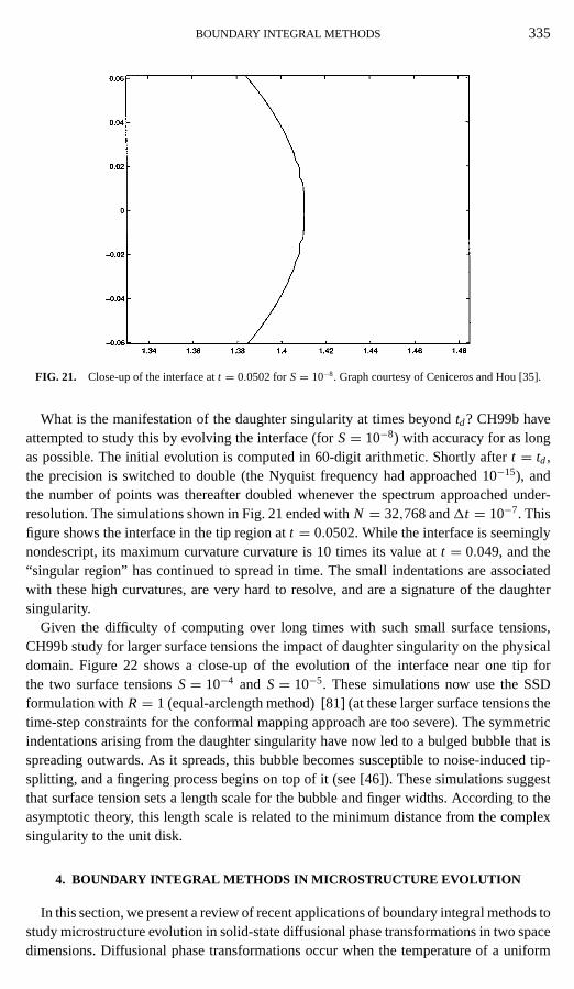
BOUNDARY INTEGRAL METHODS 335
FIG. 21. Close-up of the interface att = 0.0502 forS= 10−8. Graph courtesy of Ceniceros and Hou [35].
What is the manifestation of the daughter singularity at times beyondtd? CH99b haveattempted to study this by evolving the interface (forS= 10−8) with accuracy for as longas possible. The initial evolution is computed in 60-digit arithmetic. Shortly aftert = td,the precision is switched to double (the Nyquist frequency had approached 10−15), andthe number of points was thereafter doubled whenever the spectrum approached under-resolution. The simulations shown in Fig. 21 ended withN = 32,768 and1t = 10−7. Thisfigure shows the interface in the tip region att = 0.0502. While the interface is seeminglynondescript, its maximum curvature curvature is 10 times its value att = 0.049, and the“singular region” has continued to spread in time. The small indentations are associatedwith these high curvatures, are very hard to resolve, and are a signature of the daughtersingularity.
Given the difficulty of computing over long times with such small surface tensions,CH99b study for larger surface tensions the impact of daughter singularity on the physicaldomain. Figure 22 shows a close-up of the evolution of the interface near one tip forthe two surface tensionsS= 10−4 and S= 10−5. These simulations now use the SSDformulation withR= 1 (equal-arclength method) [81] (at these larger surface tensions thetime-step constraints for the conformal mapping approach are too severe). The symmetricindentations arising from the daughter singularity have now led to a bulged bubble that isspreading outwards. As it spreads, this bubble becomes susceptible to noise-induced tip-splitting, and a fingering process begins on top of it (see [46]). These simulations suggestthat surface tension sets a length scale for the bubble and finger widths. According to theasymptotic theory, this length scale is related to the minimum distance from the complexsingularity to the unit disk.
4. BOUNDARY INTEGRAL METHODS IN MICROSTRUCTURE EVOLUTION
In this section, we present a review of recent applications of boundary integral methods tostudy microstructure evolution in solid-state diffusional phase transformations in two spacedimensions. Diffusional phase transformations occur when the temperature of a uniform

336 HOU, LOWENGRUB, AND SHELLEY
FIG. 22. Close-ups of the Hele-Shaw interface at different times forS= 10−4 (t = 0.23–0.50, with a 0.03time difference between profiles) andS= 10−5 (t = 0.05–0.09, with a 0.01 time difference between profiles).Computation performed with the equal-arclength method. (cf. Fig. 11 of Siegelet al. [179].) Graph courtesy ofCeniceros and Hou [35].
mixture of materials is lowered into a regime where the mixture becomes unstable. Thesystem responds by nucleating second-phase precipitates surrounded by a nearly uniformmatrix. See Fig. 23 for a sketch of a typical model domain.
The precipitates evolve via the long-range diffusion of matter among the distinct crystalphases until equilibrium is re-established or diffusion is stopped by further lowering oftemperature. Many important structural materials such as steels and nickel and aluminumalloys are produced in this way. Microstructure, the detailed arrangement of distinct con-stituents on the microscopic level, is a critical variable that sets the macroscopic stiffness,strength and toughness of an alloy. Because of the industrial importance of diffusional
FIG. 23. A two-phase domain with three precipitates (p = 3).
BOUNDARY INTEGRAL METHODS 337
phase transformations, there have been many research studies to model and characterizethe transformation process.
One of the central assumptions of mathematical models of diffusional phase transforma-tions is that the system evolves so as to decrease the total energy. This energy consists ofan interfacial part, associated with the precipitate/matrix interfaces, and a bulk part due tothe elasticity of the constituent materials. As we will see, simulating the evolution processinvolves solving both a harmonic and a biharmonic-like equation for the (quasi-steady)diffusion and elastic fields respectively. The motion of interfaces is strongly mediated bysurface tension between the different phases. Consequently, many of the ideas and methodsdeveloped in the fluid dynamic context may be applied directly in this materials sciencecontext.
In the absence of the elastic stress, interfacial area is reduced by the diffusion of matterfrom regions of high interfacial curvature to regions of low curvature. This results in thegrowth of large precipitates at the expense of small ones and is known as Ostwald ripening(coarsening) [141]. This coarsening process may severely degrade the properties of thealloy. In the early 1960s, an asymptotic theory was developed by Lifshitz and Slyosov[117] and Wagner [205] (LSW) to predict the temporal power law of precipitate growthand a scaling behavior of the distribution of the droplet radius in the long time limit. Inthe LSW theory, the average precipitate radius〈R〉∼ t1/3 at long times. The LSW theoryhas two major restrictions, however. First, precipitates are assumed to be circular (sphericalin 3-D) and second, the theory is valid only in the zero precipitate volume fraction limit.Extending the results of LSW to more realistic physical situations has been a subject ofintense research interest. See the reviews by Johnson and Voorhees [92] and Voorhees [201,202] for a collection of recent references.
In this section, we discuss recent research (using the boundary integral numerical method)that has been performed to investigate diffusional evolution in systems in which the pre-cipitate/matrix boundaries are unconstrained, the precipitate volume fraction may be finiteand elastic effects may be considered. Because of space limitations, we will focus on onlya few works which we consider to be representative of state-of-the-art research in this field.
We note that because the bulk elastic energy does not necessarily favor large precipitatesover smaller ones, the coarsening process is affected most significantly by elastic stress. Thisis also confirmed experimentally as transitions from spherical to cuboidal to plate-shapedprecipitates, alignment of precipitates along specific crystallographic directions and mergingand splitting of precipitates are all observed [6, 38, 122, 130, 193, 217]. In fact, precipitatesplitting can actually lead to a decrease in average precipitate size over time. Thus, one ofthe goals of this line of research is to use elastic stress to control the evolution process so asto achieve desirable microstructures. Consequently, here we will focus primarily on workswhich consider the effect of elasticity on the diffusional evolution.
4.1. Historical Perspective
The numerical study of coarsening using the boundary integral method with arbitrarilyshaped precipitates began with a study of purely quasi-steady diffusional evolution (i.e., noelastic stress) by McFaddenet al. [126, 203]. Since then, other boundary integral methodsfor quasi-steady diffusional evolution, in the absence of elastic stress, have been developedby Akaiwa and Meiron [1], Imaeda and Kawasaki [90], Yokoyama and Sekerka [216], andZhuet al. [219], among others.

338 HOU, LOWENGRUB, AND SHELLEY
The study of elastic effects in diffusional phase transformations using the boundary in-tegral method (with arbitrary precipitate shapes) began with the work of Voorheeset al.(VMJ92) [204], who studied the evolution toward equilibrium of isolated precipitates in acubic anisotropichomogeneouselastic medium. That is, the elastic constants of the pre-cipitate and matrix are identical. More extensive simulations of microstructure evolution inhomogeneous elastic media were later performed by Su and Voorhees [182, 183] and Thorn-tonet al.(TAV99) [190]. In addition, Thompsonet al.(TSV94) [188] implemented a novelboundary integral method to calculate equilibrium precipitate shapes and their stability, inhomogeneous media, without resorting to evolution.
The study of elasticinhomogeneityin diffusional phase transformations began with thework of Jouet al. (JLL97) [93], who studied the evolution of precipitate/matrix systemsin isotropic media. Boundary integral simulations in anisotropic, inhomogeneous elasticmedia were first performed by Schmidt and Gross [168] and Schmidtet al. [169]. Theseauthors studied equilibrium precipitate shapes and their stability using a method analogousto that used by TSV94 in the homogeneous case (i.e., no time evolution). Later, Leoet al.(LLN00) [112] developed a boundary integral method to study diffusional evolution inanisotropic, inhomogeneous media.
Before we turn to a discussion of specific work, we comment that microstructure evolutionin diffusional phase transformations has also been studied using other numerical approaches,in both two and three dimensions, such as phase-field modeling (e.g., [99, 110, 114, 115,125, 140, 162, 186, 206–208] among others) and discrete atom methods (e.g., [107–109]).Further, in 3 space dimensions, there has been very recent research on diffusional evolutionin homogeneous and inhomogeneous elastic media by Thompson and Voorhees [187] andMueller and Gross [133], respectively, using boundary integral methods.
4.2. The Model
The model of microstructural evolution we review here consists of diffusionally growing,arbitrarily shaped precipitatesÄi , wherei = 1, . . . p and p is the total number of precip-itates, in an elastically stressed matrixÄM . The matrix domainÄM may be finite, infiniteor periodically arranged in the plane with the latter two being the most popular choices.We will consider infiniteÄM and we refer the reader to [72, 133, 168, 169] for discussionsof the periodic cases. Further, the equations we present are nondimensional and we use thenotation and nondimensionalization of LLN00.
Diffusion of a composition fieldc is assumed to occur in the matrix phase only and istaken to be quasi-steady:
1c = 0 in ÄM . (49)
The precipitate/matrix interfaces,0i , are assumed to be coherent, and upon which a gener-alized Gibbs–Thomson boundary condition is given,
c = c0 ≡ (τ + τ ′′)κ + Zgel, on 0i , (50)
whereτ = τ(θ) is the anisotropic surface tension andθ is the angle which the tangent ofthe interface makes with thex-axis (appropriate for 2-D). We takeτ + τ ′′ > 0. Further,κis the mean curvature (surface energy density),gel is the elasticity energy density which

BOUNDARY INTEGRAL METHODS 339
is given in Eq. (60). The constantZ is a measure of the relative contribution of the elasticand surface energies and scales with a characteristic size of the system such as the averageprecipitate radius.
The generalized Gibbs–Thomson boundary condition (50) for the composition field isanalogous to the Laplace–Young boundary condition for the pressure field in the fluiddynamics context. In the solid/solid context, the Gibbs–Thomson boundary condition wasderived by Johnson and Alexander [91], Larch`e and Cahn [106], and Leo and Sekerka [113],among others (see also [78]). Roughly speaking, this boundary condition reflects the ideathat changing the shape of a precipitate changes both the surface energy and the elasticenergy of the system.
We will also allow a finite mass flux into the system through the far-field condition
−J = limR∞→∞
1
2π
∫0∞∇c · n ds, (51)
where J is the total mass flux into the system and0∞ is a circular far-field boundarywhose radius isR∞ andn is the outward pointing normal vector. IfJ > 0, the total areaof precipitates increases with time (growth). IfJ = 0, then the total area remains fixed(equilibration or coarsening).
The normal velocityV of each precipitate–matrix interface0i is computed through aflux balance at the interface,
V = ∇c · n|0, (52)
wheren is the normal vector pointing intoÄm.We note that an analogy may be made between the diffusion problem here (withZ = 0)
and the Hele-Shaw problem described in Section 3. In the Hele-Shaw problem, the pressurep is the harmonic field, and the velocity is proportional to∇ p · n through Darcy’s law.Consequently, the surface tension enters both systems in exactly the same way. Therefore,the difficulties associated with tracking interfaces in a Hele-Shaw cell also arise in thismaterials science context.
Finally, it remains to determine the elastic energy densitygel. To calculategel, the elasticfields must be computed at each interface0i . The elastic fields arise because of misfit strainsbetween the precipitate and matrix phases as well as far-field applied strains. Following thenotation used in [112], misfit is taken into account through the constitutive relations betweenthe stress6 and the strainE . In each precipitate,
6P = CP(E P − ET ) (53)
whereET denotes the misfit strain, while in the matrix,
6M = CMEM . (54)
In the remainder of this section, we denote the precipitate and matrix phases by thesuperscriptsP and M , respectively. Although the precipitates need not have the sameelastic constants, we will make that assumption here for simplicity. In Eqs. (53) and (54),Cdenotes the orthotropic stiffness tensor, which using compact notation in two dimensions,
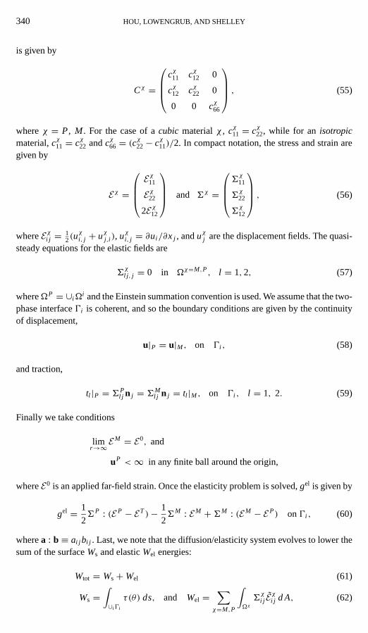
340 HOU, LOWENGRUB, AND SHELLEY
is given by
Cχ =
cχ11 cχ12 0
cχ12 cχ22 0
0 0 cχ66
, (55)
whereχ = P, M . For the case of acubic materialχ , cχ11 = cχ22, while for an isotropicmaterial,cχ11 = cχ22 andcχ66 = (cχ22− cχ11)/2. In compact notation, the stress and strain aregiven by
Eχ =
Eχ11
Eχ22
2Eχ12
and 6χ =
6χ11
6χ22
6χ12
, (56)
whereEχi j = 12(u
χi, j + uχj,i ), uχi, j = ∂ui /∂xj , anduχj are the displacement fields. The quasi-
steady equations for the elastic fields are
6χl j , j = 0 in Äχ=M,P, l = 1, 2, (57)
whereÄP = ∪iÄi and the Einstein summation convention is used. We assume that the two-
phase interface0i is coherent, and so the boundary conditions are given by the continuityof displacement,
u|P = u|M , on 0i , (58)
and traction,
tl |P = 6Pl j n j = 6M
l j n j = tl |M , on 0i , l = 1, 2. (59)
Finally we take conditions
limr→∞ E
M = E0, and
uP <∞ in any finite ball around the origin,
whereE0 is an applied far-field strain. Once the elasticity problem is solved,gel is given by
gel = 1
26P : (E P − ET )− 1
26M : EM +6M : (EM − E P) on0i , (60)
wherea : b ≡ ai j bi j . Last, we note that the diffusion/elasticity system evolves to lower thesum of the surfaceWs and elasticWel energies:
Wtot = Ws+Wel (61)
Ws =∫∪i0i
τ(θ) ds, and Wel =∑
χ=M,P
∫Äχ6χi j E
χi j d A, (62)
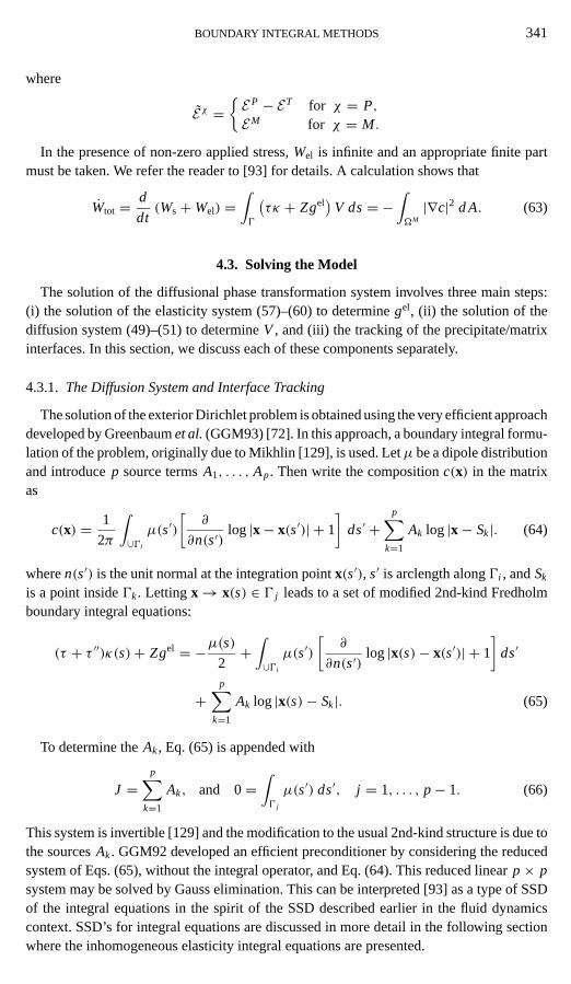
BOUNDARY INTEGRAL METHODS 341
where
Eχ ={E P − ET for χ = P,EM for χ = M.
In the presence of non-zero applied stress,Wel is infinite and an appropriate finite partmust be taken. We refer the reader to [93] for details. A calculation shows that
Wtot = d
dt(Ws+Wel) =
∫0
(τκ + Zgel
)V ds= −
∫ÄM
|∇c|2 d A. (63)
4.3. Solving the Model
The solution of the diffusional phase transformation system involves three main steps:(i) the solution of the elasticity system (57)–(60) to determinegel, (ii) the solution of thediffusion system (49)–(51) to determineV , and (iii) the tracking of the precipitate/matrixinterfaces. In this section, we discuss each of these components separately.
4.3.1. The Diffusion System and Interface Tracking
The solution of the exterior Dirichlet problem is obtained using the very efficient approachdeveloped by Greenbaumet al.(GGM93) [72]. In this approach, a boundary integral formu-lation of the problem, originally due to Mikhlin [129], is used. Letµ be a dipole distributionand introducep source termsA1, . . . , Ap. Then write the compositionc(x) in the matrixas
c(x) = 1
2π
∫∪0i
µ(s′)[
∂
∂n(s′)log |x− x(s′)| + 1
]ds′ +
p∑k=1
Ak log |x− Sk|. (64)
wheren(s′) is the unit normal at the integration pointx(s′), s′ is arclength along0i , andSk
is a point inside0k. Lettingx→ x(s) ∈ 0 j leads to a set of modified 2nd-kind Fredholmboundary integral equations:
(τ + τ ′′)κ(s)+ Zgel = −µ(s)2+∫∪0i
µ(s′)[
∂
∂n(s′)log |x(s)− x(s′)| + 1
]ds′
+p∑
k=1
Ak log |x(s)− Sk|. (65)
To determine theAk, Eq. (65) is appended with
J =p∑
k=1
Ak, and 0=∫0 j
µ(s′) ds′, j = 1, . . . , p− 1. (66)
This system is invertible [129] and the modification to the usual 2nd-kind structure is due tothe sourcesAk. GGM92 developed an efficient preconditioner by considering the reducedsystem of Eqs. (65), without the integral operator, and Eq. (64). This reduced linearp× psystem may be solved by Gauss elimination. This can be interpreted [93] as a type of SSDof the integral equations in the spirit of the SSD described earlier in the fluid dynamicscontext. SSD’s for integral equations are discussed in more detail in the following sectionwhere the inhomogeneous elasticity integral equations are presented.

342 HOU, LOWENGRUB, AND SHELLEY
The implementation used by GGM93 to solve Eqs. (64)–(65) is highly accurate andefficient. The integrals are discretized with spectral accuracy using the trapezoid rule andthe fast multipole method (FMM) [31, 74] is used to evaluate the discrete sums inO(N)work. The iterative method GMRES [163] is then used to solve the discrete matrix system.Thus, the methods of GGM make it possible to solve the exterior diffusion problem for manymore precipitates than was previously computationally affordable. With this improvement,interface tracking then becomes the limiting computational step in the simulation of purediffusional systems.
Using the dipole formulation of GGM93, the normal velocity is given by
Vi (s)= 1
2π
∫∪0 j
µs′∂
∂slog|x(s)−x(s′)| ds′+
p∑k=1
Ak
(x1(s)−xs
1k
)x2,s−
(x2(s)−xs
2k
)x1,s(
x1(s)− xs1k
)2+ (x2(s)− xs2k
)2 ,
(67)
where the integral is interpreted in the principal value sense. A spectrally accurate dis-cretization of this integral is obtained using the alternate point trapezoidal rule analogousto that given in Eq. (36). Because of the third-order time-step constraint due to the surfacetension (e.g., see Eq. (41)), interface tracking remained a problem for these systems untilthe recent work of HLS94. Their SSD applies directly to the diffusional system since
V ∼ 1
2H[(τ + τ ′′)κ],s (68)
at small spatial scales [81, 82, 93, 112], since the surface energy dominates the elastic energyat these scales. If one writesτ + τ ′′ = 1+ (τ0+ τ ′′0 ), then one can follow the approachoutlined previously for the Hele-Shaw case [81] and rewrite the interface evolution equationsX = Vn+ Ts using the tangent angleθ and equal arclength tangential velocityT . Notethat the equations are exactly as in the Hele-Shaw case (Eq. 42) except that the definition ofN now includes the anisotropic surface energy. Except for the anisotropic surface energycontribution, the remainder termsN are lower order at small spatial scales. Although thesurface energy termH[(τ0+ τ ′′0 )θi,αα],α is of the same order as the termH(θi,ααα), it wasfound by Almgrenet al.[4] and LLN00 that the splitting in Eq. (42) is effective in removingthe stiffness numerically provided thatτ0+ τ ′′0 is smooth and not too close to 1.
At this point, we can discuss simulations of purely diffusional evolution in the absence ofelastic stress (Z = 0). In metallic alloy systems, this corresponds to simulating systems ofvery small precipitates where the surface energy dominates the elastic energy. The currentstate of the art in solving the pure diffusional evolution problem is the work of Akaiwa andMeiron (AM96) [1]. AM96 combined the modified dipole approach of GGM93 togetherwith the non-stiff time stepping of HLS94 to study the coarsening behavior of large precip-itate/matrix systems with isotropic surface tension (τ0 = 0). AM96 performed simulationscontaining over 5000 precipitates initially. Precipitates are removed if their area decreasesbelow a certain tolerance. We note that the effect of removing precipitates was analyzedin [93] (elasticity was also considered). To make such large computations feasible, AM96also took into account the effectively finite interaction distance of the diffusion field. Forinstance, particle–particle diffusional interactions may be neglected with only small relativeerrors if the particles are well enough separated [1]. To take advantage of this fact, AM96divided the computational unit cell into sub-cells each containing 50–150 precipitates. In-side each sub-cell, the full diffusion field is computed. The influence of particles outside
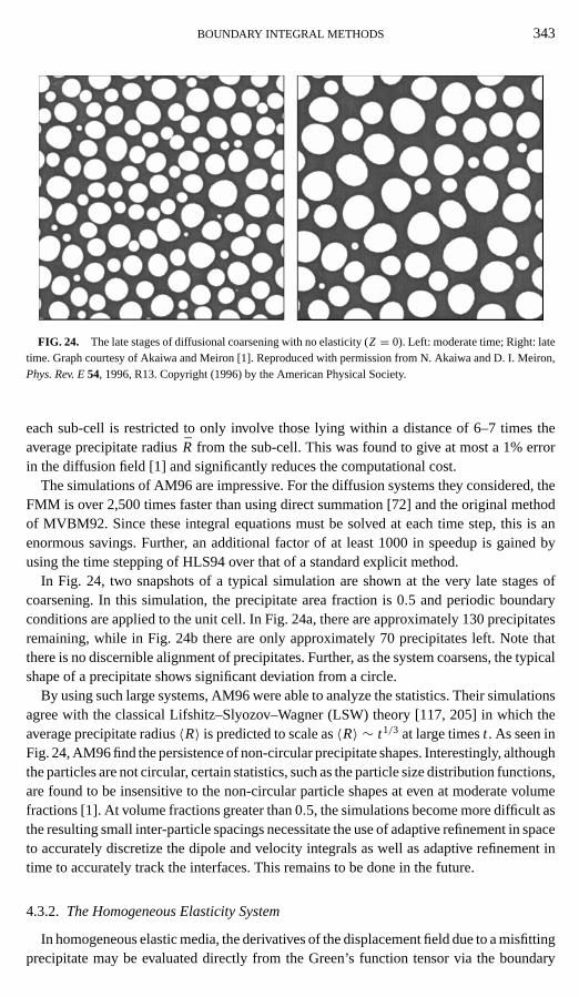
BOUNDARY INTEGRAL METHODS 343
FIG. 24. The late stages of diffusional coarsening with no elasticity (Z = 0). Left: moderate time; Right: latetime. Graph courtesy of Akaiwa and Meiron [1]. Reproduced with permission from N. Akaiwa and D. I. Meiron,Phys. Rev. E54, 1996, R13. Copyright (1996) by the American Physical Society.
each sub-cell is restricted to only involve those lying within a distance of 6–7 times theaverage precipitate radiusR from the sub-cell. This was found to give at most a 1% errorin the diffusion field [1] and significantly reduces the computational cost.
The simulations of AM96 are impressive. For the diffusion systems they considered, theFMM is over 2,500 times faster than using direct summation [72] and the original methodof MVBM92. Since these integral equations must be solved at each time step, this is anenormous savings. Further, an additional factor of at least 1000 in speedup is gained byusing the time stepping of HLS94 over that of a standard explicit method.
In Fig. 24, two snapshots of a typical simulation are shown at the very late stages ofcoarsening. In this simulation, the precipitate area fraction is 0.5 and periodic boundaryconditions are applied to the unit cell. In Fig. 24a, there are approximately 130 precipitatesremaining, while in Fig. 24b there are only approximately 70 precipitates left. Note thatthere is no discernible alignment of precipitates. Further, as the system coarsens, the typicalshape of a precipitate shows significant deviation from a circle.
By using such large systems, AM96 were able to analyze the statistics. Their simulationsagree with the classical Lifshitz–Slyozov–Wagner (LSW) theory [117, 205] in which theaverage precipitate radius〈R〉 is predicted to scale as〈R〉 ∼ t1/3 at large timest . As seen inFig. 24, AM96 find the persistence of non-circular precipitate shapes. Interestingly, althoughthe particles are not circular, certain statistics, such as the particle size distribution functions,are found to be insensitive to the non-circular particle shapes at even at moderate volumefractions [1]. At volume fractions greater than 0.5, the simulations become more difficult asthe resulting small inter-particle spacings necessitate the use of adaptive refinement in spaceto accurately discretize the dipole and velocity integrals as well as adaptive refinement intime to accurately track the interfaces. This remains to be done in the future.
4.3.2. The Homogeneous Elasticity System
In homogeneous elastic media, the derivatives of the displacement field due to a misfittingprecipitate may be evaluated directly from the Green’s function tensor via the boundary

344 HOU, LOWENGRUB, AND SHELLEY
integral
u j,k(x) = (Ci j 11+ εr Ci j 22)
∫0
gi j ,k(x, x′)n′l ds′, (69)
wherex is either in the matrix or in the precipitate and
Ci jkl = 2c66δikδ j l + c12δi j δkl − (c11− c12− 2c66)δi jkl ,
for cubic systems; here we do not use compact notation. The misfit tensorET is assumedto take the form
ET =(
1 00 εr
), (70)
whereεr is a constant. In two space dimensions, one may find an effectively analyticform for gi j ,k that depends on the anisotropy ratioA = 2c66/(c11− c12). Taking the limitasx→ x(s) ∈ 0, the result involves a rather complicated principal value integral whoseexact form we do not present here; we instead refer the reader to [182, 183, 188, 204]. Wenote thatgel is easily constructed onceu j,k has been obtained (also see [204] for example).
The current state of the art in simulating diffusional evolution in homogeneous, anisotropicelastic media is the recent work of Thorntonet al. (TAV99) [189–191] in which the coars-ening of large cubic systems is studied. In metallic alloys, such a system can be consideredas a model for nickel–aluminum alloys, since in those alloys the precipitates and matrixboth have face-centered-cubic lattices with elastic constants typically differing by less than10% [122]. TAV99 combined the improvements in interface tracking due to HLS94 andin the diffusion solver due to AM96 and GGM93. In addition, TAV99 developed a fastmultipole method to evaluate the elasticity integral in Eq. (69). With these improvements,TAV99 achieved an enormous gain in computational efficiency and are now able to analyzethe statistics of microstructure evolution in homogeneous elastic media.
In preliminary work, TAV99 have performed simulations involving over 4000 precipitatesinitially. As in AM96, precipitates are removed when their area reaches a certain lowertolerance. See Fig. 25 for results withZ = 2.0, 4.1 and 6.1 and with isotropic surfacetension and dilatational misfits. The value ofZ is allowed to vary dynamically throughan average precipitate radius. Thus, as precipitates coarsen and grow larger,Z increasescorrespondingly. The initial volume fraction of precipitates is 0.1 and simulations are startedwith Z = 1. TAV99 find that the morphological evolution is significantly different in thepresence of elastic stress. Unlike the purely diffusional case and consistent with experimentalresults, large-scale alignment of particles is seen in the〈100〉 and〈010〉 directions duringthe evolution process. In addition, there is significant shape dependence as nearly circularprecipitates are seen at smallZ = 2.0, while at Z = 4.1 and Z = 6.1, precipitates aresquarish and rectangular, respectively. As in AM96, certain features of the process areinsensitive to the shape variation and work is continuing to determine the asymptotic rateof increase of〈R〉 in time.
4.3.3. The Inhomogeneous Elasticity System
While the elastic constants of the nickel–aluminum precipitates and a nickel matrix maydiffer by only 10%, there are other nickel-based alloys in which the elastic constants may

BOUNDARY INTEGRAL METHODS 345
FIG. 25. Coarsening in homogeneous, cubic elasticity. Upper graph: early time (Z = 2.0); Middle graph:moderate time (Z = 4.1); lower graph: late time (Z = 6.1). Graph courtesy of Thornton, Akaiwa, and Voorhees[190].
differ by more than 50%. Examples of such systems include nickel–silicon and nickel–gallium precipitates in a nickel matrix. It therefore is important to be able to account forelastic inhomogeneity. Indeed, the results of many investigations now indicate that evensmall elastic inhomogeneities may significantly impact precipitate evolution (e.g., [93, 112,114, 115, 140, 162, 168, 169]).
The inhomogeneous elasticity system (57)–(60) is much more difficult to solve thanthe homogeneous system. Unlike the homogeneous case, integral equations must now besolved in order to obtain the inhomogeneous elastic fields. The elasticity system (57)–(60)may be reformulated in terms of boundary integrals as follows. Letui (s) andti (s) be thecomponents of displacement and traction on the boundary, respectively. One may then usea direct approach, involving both elastic monopoles and dipoles, to obtain a system of four

346 HOU, LOWENGRUB, AND SHELLEY
coupled integral equations for the displacement and traction components on each interface0,
u j (s)
2+∫0
uk(s′)T P
kj (x(s), x(s′)) ds′ −
∫0
tk(s′)U P
kj (x(s), x(s′)) ds′
=∫0
t Tk (s′)U P
kj (z(s), z(s′)) ds′, (71)
− u j (s)
2+∫0
uk(s′)T M
kj (x(s), x(s′)) ds′ −
∫0
tk(s′)U M
kj (x(s), x(s′)) ds′
= − uAj (x(s))
2
∫0
uAk (s′)T M
kj (x(s), x(s′)) ds′ −
∫0
t Ak (s′)U P
kj (x(s), x(s′)) ds′, (72)
where0 = ∪i0i andU P(x, x′), U M(x, x′) are the fundamental solution tensors in the pre-cipitate and matrix domains (considered separately) that generate displacement vectorsu j (x) arising from an isolated point source located atx′ in the precipitate and the matrixrespectively. In Eq. (72),T P andT M are the analogous traction tensor fields. We do not givethe exact form ofUχ andTχ here; instead we refer the reader to JLL97 for the isotropiccase and LLN00 for the orthotropic case (see also [153, 154, 168, 169]). TheUχ containsboth smooth and logarithmic functions while theTχ contains both smooth functions andfunctions with Cauchy-type singularities; theTχ integrals are interpreted in the principalvalue sense. Finally, in Eqs. (71) and (72),tT is the traction vector due to the misfit strainin the precipitatetT = CET anduA andt A are the displacement and traction vectors of aconstant applied stress field6A.
The small scale decomposition for integral equations.Although the system (71), (72)is a Fredholm equation of mixed type with smooth, logarithmic, and Cauchy-type kernels,it was shown by JLL97, in the isotropic case, and by LLN00, in the anisotropic case, that itmay be transformed directly to a second kind Fredholm system with smooth kernels. Thetransformation relies on an analysis of the equations at small spatial scales and is in spiritlike the SSD in the fluid dynamic context. Classical Fredholm theory [152] may be usedto guarantee the existence and uniqueness of solutions since the displacement is uniquelyspecified at infinity (uA).
If Eqs. (71) and (72) are discretized directly, the condition numbers increase at leastlinearly with N (the total number of points) due to the logarithmic kernels. The conditionnumber also increases slowly as the number of precipitatesp increases. To overcome thisill-conditioning, JLL97 and LLN00 performed a small scale analysis of the equations todetermine the dominant terms at small scales in the spirit of HLS94. For example, supposea system of integral equations may be written as
A[u, t] = f (73)
and suppose thatA ∼ L at high wave-numbers, while the remainder involves integrationagainst smooth kernels. Then one may write
A = L+R. (74)
If L is diagonalizable in Fourier space, and so is easily inverted using the FFT, one mayrewrite Eq. (73) as
(I + L−1R)[u, t] = L−1f, (75)

BOUNDARY INTEGRAL METHODS 347
which is a second-kind Fredholm equation. When discretized, Eq. (75) is well conditioned[93]. See [219], for example, for an application to a first-kind Fredholm equation for theDirichlet problem.
Application to the inhomogeneous elasticity integral equations.In the elasticity case,the SSD reveals that the dominant operator at small scales is
L = (L1,1,1, . . . ,L1,1,p,L1,2,1, . . . ,L1,2,p,L2,1,L2,2), (76)
where the components ofL are then given by
L1,l , j [u, t] = 1
2ul − DP
1lkH[uk] − DP2lkH[ t k], (77)
L2,l [u, t] = 1
2ul − DP
1lkH[uk] − DM2lkH[ t k], (78)
and ∂α t k = L j tk/2π and DP,M1,2 depend only on the elastic constants (see [93, 112] for
details). Note that theuk and t k that appear on the right hand sides of Eqs. (77) and(78) are only evaluated on0 j . In contrast,A involves evaluation ofuk and tk on all theprecipitate/matrix interfaces∪ j0 j . AlthoughL is a nonlocal operator, solving
L[u, t] = b
only involves inverting a 4× 4 matrix in Fourier space sinceL is diagonalized by the Fouriertransform. This ismuchsimpler than solving the full system. Further, if the precipitate/matrixboundaries are smooth, then the remainder operatorR involves integration against smoothkernels and thus is a smoothing operator. Roughly speaking, this means that as an operator,R has a rapidly decaying Fourier symbol [93]. This type of small scale decompositionfor integral equations obviates the need to use Goursat functions to formulate second-kindequations directly for the elasticity system [73, 129]. Typically, this SSD preconditioningreduces the iteration count by about a factor of about 5 over that for the unpreconditionedsystem [93, 112]. What remains of the original ill-conditioning is thatL−1 ∼ |k| for largewave-numbersk. Thus, numerical errors inf are amplified by the application ofL−1.Numerical filtering [81, 104] is used to control this amplification.
We remark that Greengard and Helsing (GH98) [73] have recently developed a fastalgorithm for computing elastic fields in isotropic, inhomogeneous elastic media. Theiralgorithm is based on an indirect integral equation approach using complex potentials,due to Sherman [177], combined with the fast multipole method and adaptive Gauss–Legendre quadrature. In this approach, a single second kind Fredholm equation for eachinterface is obtained directly for a Cauchy layer potential. This alone presents an enormoussavings over the direct approach discussed where four equations must be solved for eachinterface. However, the methods of GH98 currently only account for applied fields andnot for precipitate misfit strains. Nevertheless, this approach is very promising for use inmicrostructure evolution and Helsing and Lowengrub are studying its extension to the caseof misfitting precipitates.
4.3.4. Interface Tracking in the Face of Anisotropy
LLN00 observed that certain microscopic details of the numerical solution, such asc0, may depend sensitively on the numerical time-integration algorithms. This sensitive
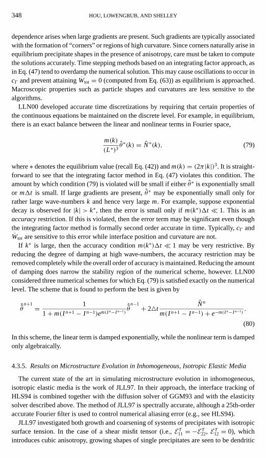
348 HOU, LOWENGRUB, AND SHELLEY
dependence arises when large gradients are present. Such gradients are typically associatedwith the formation of “corners” or regions of high curvature. Since corners naturally arise inequilibrium precipitate shapes in the presence of anisotropy, care must be taken to computethe solutions accurately. Time stepping methods based on an integrating factor approach, asin Eq. (47) tend to overdamp the numerical solution. This may cause oscillations to occur inc0 and prevent attainingWtot = 0 (computed from Eq. (63)) as equilibrium is approached.Macroscopic properties such as particle shapes and curvatures are less sensitive to thealgorithms.
LLN00 developed accurate time discretizations by requiring that certain properties ofthe continuous equations be maintained on the discrete level. For example, in equilibrium,there is an exact balance between the linear and nonlinear terms in Fourier space,
m(k)
(L∗)3θ∗(k) = N∗(k), (79)
where∗ denotes the equilibrium value (recall Eq. (42)) andm(k) = (2π |k|)3. It is straight-forward to see that the integrating factor method in Eq. (47) violates this condition. Theamount by which condition (79) is violated will be small if eitherθ∗ is exponentially smallor m1t is small. If large gradients are present,θ∗ may be exponentially small only forrather large wave-numbersk and hence very largem. For example, suppose exponentialdecay is observed for|k| > k∗, then the error is small only ifm(k∗)1t ¿ 1. This is anaccuracyrestriction. If this is violated, then the error term may be significant even thoughthe integrating factor method is formally second order accurate in time. Typically,c0 andWtot are sensitive to this error while interface position and curvature are not.
If k∗ is large, then the accuracy conditionm(k∗)1t ¿ 1 may be very restrictive. Byreducing the degree of damping at high wave-numbers, the accuracy restriction may beremoved completely while the overall order of accuracy is maintained. Reducing the amountof damping does narrow the stability region of the numerical scheme, however. LLN00considered three numerical schemes for which Eq. (79) is satisfied exactly on the numericallevel. The scheme that is found to perform the best is given by
ˆθn+1 = 1
1+m(I n+1− I n−1)em(I n−I n−1)
ˆθn−1+ 24t
Nn
m(I n+1− I n−1)+ e−m(I n−I n−1).
(80)
In this scheme, the linear term is damped exponentially, while the nonlinear term is dampedonly algebraically.
4.3.5. Results on Microstructure Evolution in Inhomogeneous, Isotropic Elastic Media
The current state of the art in simulating microstructure evolution in inhomogeneous,isotropic elastic media is the work of JLL97. In their approach, the interface tracking ofHLS94 is combined together with the diffusion solver of GGM93 and with the elasticitysolver described above. The method of JLL97 is spectrally accurate, although a 25th-orderaccurate Fourier filter is used to control numerical aliasing error (e.g., see HLS94).
JLL97 investigated both growth and coarsening of systems of precipitates with isotropicsurface tension. In the case of a shear misfit tensor (i.e.,ET
11 = −ET22, ET
12 = 0), whichintroduces cubic anisotropy, growing shapes of single precipitates are seen to be dendritic

BOUNDARY INTEGRAL METHODS 349
FIG. 26. A series of different precipitate shapes under growth conditions in isotropic, inhomogeneous elasticmedia with shear misfit. In (a)–(c), the flux isJ = 10. In (a), the shear modulus of the precipitate is twice that ofthe matrix. In (b), the opposite case is shown. In (c), there is no elasticity (Z = 0). In (d), the nonconvex shape isfrom (a) at timet = 20, whereas the convex shape is the corresponding equilibrium shape. Graph courtesy of Jouet al. [93].
while equilibrium shapes are squarish. See Fig. 26 for a sample of results. In (a) and (b), thenumerical flux isJ = 10. In (a), the shear modulus of the precipitate is half of that ofthe matrix (soft precipitate) while the opposite is true in (b) (hard precipitate). Note thatthe dendrite arms are more slender for the soft precipitate than for the hard precipitate.In addition, wiggles form on the dendrite arms of the soft precipitate, which indicatesadditional instability in the soft case relative to the hard. We also note that the observeddendritic structure in both cases qualitatively resembles that obtained using no elasticity(Z = 0), but anisotropic surface tension [4] (see Fig. 14). In Fig. 26e, the correspondingcase with isotropic surface tension andZ = 0 is shown. Note the isotropic nature of thecurve, as well as the occurrence of tip splitting, is suppressed by the elasticity. In Fig. 26d,the convex curve corresponds to the equilibrium precipitate shape obtained by settingJ = 0at t = 20 for the soft precipitate (the non-convex shape shown in the figure).
In Fig. 27, a sample simulation is shown of 16 precipitates coarsening (J = 0) in inhomo-geneous, isotropic elastic media. Precipitates are removed when their area drops below 0.1.Because of the isotropic surface tension and choice of misfit (tetragonal withET
11 6= ET22 > 0,
ET12 = 0), the precipitates develop roughly elliptical shapes. An overall classical coarsening
behavior occurs as large precipitates grow at the expense of small ones. Further, over the timescales shown, there is no significant precipitate translation or alignment. Thus, it appearsthat alignment is a secondary process that occurs after shape changes and coarsening.
When precipitates are removed, the surface and elastic energies are continuous but thesurface energy is kinked. In fact, it may be shown thatWtot ∼ (tc − t)−2/3 [93]. This maybe seen explicitly in Fig. 28, whereW andW are shown for the simulation in Fig. 27. Asexpected,Wtot drops sharply just before a precipitate is removed. Because precipitates are
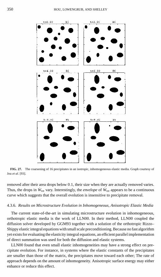
350 HOU, LOWENGRUB, AND SHELLEY
FIG. 27. The coarsening of 16 precipitates in an isotropic, inhomogeneous elastic media. Graph courtesy ofJouet al. [93].
removed after their area drops below 0.1, their size when they are actually removed varies.Thus, the drops inWtot vary. Interestingly, theenvelopeof Wtot appears to be a continuouscurve which suggests that the overall evolution is insensitive to precipitate removal.
4.3.6. Results on Microstructure Evolution in Inhomogeneous, Anisotropic Elastic Media
The current state-of-the-art in simulating microstructure evolution in inhomogeneous,orthotropic elastic media is the work of LLN00. In their method, LLN00 coupled thediffusion solver developed by GGM93 together with a solution of the orthotropic Rizzo–Shippy elastic integral equations with small scale preconditioning. Because no fast algorithmyet exists for evaluating the elasticity integral equations, an efficient parallel implementationof direct summation was used for both the diffusion and elastic systems.
LLN00 found that even small elastic inhomogeneities may have a strong effect on pre-cipitate evolution. For instance, in systems where the elastic constants of the precipitatesare smaller than those of the matrix, the precipitates move toward each other; The rate ofapproach depends on the amount of inhomogeneity. Anisotropic surface energy may eitherenhance or reduce this effect.
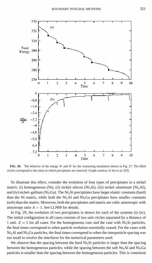
BOUNDARY INTEGRAL METHODS 351
FIG. 28. The behavior of the energyW andW for the coarsening simulation shown in Fig. 27. The filledcircles correspond to the times at which precipitates are removed. Graph courtesy of Jouet al. [93].
To illustrate this effect, consider the evolution of four types of precipitates in a nickelmatrix: (i) homogeneous (Ni), (ii) nickel–silicon (Ni3Si), (iii) nickel–aluminum (Ni3Al),and (iv) nickel–gallium (Ni3Ga). The Ni3Si precipitates have larger elastic constants (hard)than the Ni matrix, while both the Ni3Al and Ni3Ga precipitates have smaller constants(soft) than the matrix. Moreover, both the precipitates and matrix are cubic anisotropic withanisotropy ratioA > 1. See LLN00 for details.
In Fig. 29, the evolution of two precipitates is shown for each of the systems (i)–(iv).The initial configuration in all cases consists of two unit circles separated by a distance of1 unit. Z = 5 for all cases. For the homogeneous case and the case with Ni3Si particles,the final times correspond to when particle evolution essentially ceased. For the cases withNi3Al and Ni3Ga particles, the final times correspond to when the interparticle spacing wastoo small to resolve the interfaces for the numerical parameters used.
We observe that the spacing between the hard Ni3Si particles is larger than the spacingbetween the homogeneous particles, while the spacing between the soft Ni3Al and Ni3Gaparticles is smaller than the spacing between the homogeneous particles. This is consistent

352 HOU, LOWENGRUB, AND SHELLEY
FIG. 29. The behavior of two precipitates in inhomogeneous, cubic anisotropic elasticity. Graph courtesy ofLeoet al. [112].
with simulations in isotropic media where that hard particles repel, while soft particles attract[93]. However, the situation is more complex with anisotropic elasticity. In the homogeneousand the Ni3Si case, the particles move towards each other with very small velocities whichtend to zero at a finite interparticle distance. In the Ni3Ga case, the interparticle attractionincreases as the interparticle spacing decreases. This suggests the particles will merge. Inthe Ni3Al case (which is nearly homogeneous), however, the interparticle attraction beginsto decrease when the particles are very close to one another. More refined calculations arenecessary to determine whether there is in fact a small non-zero interparticle spacing inthis case. The difference between the Ni3Ga and Ni3Al cases is also reflected in the particleshapes in the interparticle region; in the Ni3Ga case, the particles appear to curve towardeach other, while in the Ni3Al case, the two particles have “squared off” against each other.
Finally, we conclude this section by presenting some recent preliminary results, obtainedby LLN00 [111], which indicate that an elastically driven morphological instability mayoccur in the presence of applied fields. Inhomogeneity plays a crucial role in the instabilityas an analogous instability has not yet been observed in homogeneous systems [111].

BOUNDARY INTEGRAL METHODS 353
FIG. 30. The elastic morphological instability of a misfiting singleNi3Si precipitate in an applied shear. In(a), Z = 5. In (b), Z = 3. In (c), a homogeneous precipitate is shown for comparison withZ = 5 andZ = 10.Graph courtesy of Leoet al. [111].
Moreover, the instability apparently leads to precipitate splitting. This may be the source ofsplitting observed in experiments [94, 217] for example. A similar morphological instabilityhas been observed in simulations using the discrete atom method [108, 109].
The elastic morphological instability may be seen in the following context. Consider theevolution of a single Ni3Si precipitate with applied shear and dilatational misfit. This isshown in Fig. 30a withZ = 5 and isotropic surface tension. In this simulation, the initialcondition is a circle. The interface is then shown at subsequent times near pinch-off. Observethat the interface forms two interpenetrating fingers that grow toward one another, stronglysuggesting that the precipitate will split into two platelike precipitates with long axes orientedin thex2-direction. There is a very slight amount of asymmetry in the plot due to numericalerror and more refined simulations are currently being performed; convergence tests atearlier times confirm that the instability is physical and not numerical. For the purposes ofcomparison, Fig. 30b shows the evolution of the precipitate withZ = 3. In this simulation,there is a hint of instability at small times although the precipitate boundary stabilizesand becomes elliptical. In Fig. 30c, the evolution of a homogeneous precipitate is shownwith Z = 5 (solid squarish line) andZ = 10 (dashed line). In the homogeneous case, the
354 HOU, LOWENGRUB, AND SHELLEY
precipitate converges to a squarish equilibrium shape which is remarkably different fromthat seen in the inhomogeneous cases.
5. CONCLUSIONS AND FUTURE DIRECTIONS
In this paper, we have presented a brief review of the application of boundary integralmethods in two dimensions to multicomponent fluid flows and multiphase problems inmaterials science. In particular, we have focused on results from the recent development ofmethods which accurately and efficiently include surface tension. In fluid flows, we haveexamined the effects of surface tension on the Kelvin–Helmholtz and Rayleigh–Taylorinstabilities, the generation of capillary waves on a free surface, and problems involvingpattern generation and selection and singularity formation in Hele-Shaw flows. In mate-rials science, we discussed microstructure evolution in diffusional phase transformationsand the effects of the resulting competition between surface and elastic energies on themicrostructure morphology.
The significant recent developments underlying these simulational studies are (i) theanalyses of BHL93/BHL96 and BN98 which identify and correct instabilities generated byspatial discretization, and most especially (ii) the introduction of the SSD by HLS94/HLS97to develop very efficient and accurate time discretization methods. Until these works, simula-tions were fraught with numerical instability and were greatly limited in accuracy and tempo-ral evolution. The above works have provided the backbone of new classes of methods whichhave enabled the study of much more complex phenomena than was previously possible.
Many challenges remain for the future. These include the extension of the ideas presentedhere to more complicated flows such as those involving viscosity and/or elastic boundaryforces (e.g., from simulations of heart function), as well as to axisymmetric and 3-D inter-face evolution. In axisymmetric flows, the SSD has recently been extended to the vortexsheet case by Nie [135], and to axisymmetric porous media flow by Ceniceros and Si [37].The development of accurate and efficient boundary integral methods for interface evolutionin 3-D is a highly non-trivial problem and has been the subject of much recent research (see,for example [20, 76, 83, 84]). The development of efficient and accurate time-stepping algo-rithms in 3-D, analogous to those in 2-D based on the SSD, is an outstanding problem. In thematerials science context, where the time-step restrictions are third-order, the developmentof efficient time integration methods is crucial. Although there have been three dimensionalboundary integral simulations recently performed by Thompson and Voorhees [187] forhomogeneous systems and by Mueller and Gross [133] for inhomogeneous systems, thoseworks were limited by spatial and temporal resolution requirements.
ACKNOWLEDGMENTS
The authors thank R. Almgren, N. Akaiwa, P. H. Leo, D. Meiron, Q. Nie, D. Thompson, K. Thornton, andP. Voorhees, who provided us with figures from their recent results. T.Y.H. acknowledges support from NSFGrant DMS-9704976 and ARO Grant DAAD19-99-1-0141 (ARO). J.L. acknowledges support from NSF GrantDMS-9706931 and from the Minnesota Supercomputer Institute. M.J.S. acknowledges support from NSF GrantDMS-9707494 and DOE Grant DE-FG02-88ER25053.
REFERENCES
1. N. Akaiwa and D. I. Meiron, Two-dimensional late-stage coarsening for nucleation and growth at high-areafractions,Phys. Rev. E54, R13 (1996).

BOUNDARY INTEGRAL METHODS 355
2. R. Almgren, Singularity formation in Hele-Shaw bubbles,Phys. Fluids8, 344 (1996).
3. R. Almgren, A. Bertozzi, and M.P. Brenner, Stable and unstable singularities in the unforced Hele-Shawcell, Phys. Fluids8, 1356 (1996).
4. R. Almgren, W.-S. Dai, and V. Hakim, Scaling behavior in anisotropic Hele-Shaw flow,Phys. Rev. Lett.71,3461 (1993).
5. C. Anderson, A vortex method for flows with slight density variations,J. Comput. Phys.61, 417 (1985).
6. A. J. Ardell and R. B. Nicholson, On the modulated structure of aged Ni–Al alloys,Acta Metall.14, 1295(1966).
7. A. Arneodo, Y. Couder, G. Grasseau, V. Hakim, and M. Rabaud, Uncovering the analytical Saffman–Taylorfinger in unstable viscous fingering and diffusion-limited aggregation,Phys. Rev. Lett.63, 984 (1989).
8. U. Ascher, S. Ruuth, and B. Wetton, Implicit–explicit methods for time-dependent partial differential equa-tions,SIAM J. Numer. Anal.32, 797 (1995).
9. D. H. Bailey,MPFUN: A Portable High Perfomance Multiprecision Package, Technical Report RNR-90-022,(NASA Ames Research Center, 1990).
10. G. Baker, D. Meiron, and S. Orszag, Boundary integral methods for axisymmetric and 3-dimensionalRayleigh–Taylor instability problems,Physica D12, 19 (1984).
11. G. Baker and A. Nachbin, Stable methods for vortex sheet motion in the presence of surface tension,SIAMJ. Sci. Comput.19, 1737 (1998).
12. G. Baker, M. Siegel, and S. Tanveer, A well-posed numerical method to track isolated conformal-mapsingularities in Hele-Shaw flow,J. Comput. Phys.120, 348 (1995).
13. G. R. Baker, D. I. Meiron, and S. A. Orszag, Vortex simulations of the Rayleigh–Taylor instability,Phys.Fluids23, 1485 (1980).
14. G. R. Baker, D. I. Meiron, and S. A. Orszag, Generalized vortex methods for free-surface flow problems,J. Fluid Mech.123, 477 (1982).
15. G. R. Baker and D. W. Moore, The rise and distortion of a two dimensional gas bubble in an inviscid fluid,J. Fluid Mech.123, 477 (1982).
16. G. R. Baker and Q. Nie, The asymptotic motion of an accelerating, thick layer of inviscid fluid,Phys. Fluids10, 101 (1998).
17. G. R. Baker and M. J. Shelley, On the connection between thin vortex layers and vortex sheets,J. FluidMech.215, 161 (1990).
18. J. Beale, T. Hou, and J. Lowengrub, Growth rates for the linear motion of fluid interfaces far from equilibrium,Comm. Pure Appl. Math.46, 1269 (1993).
19. J. Beale, T. Hou, and J. Lowengrub, Convergence of a boundary integral method for water waves,SIAM J.Numer. Anal.33, 1797 (1996).
20. J. T. Beale, A convergent boundary integral method for 3-D water waves,Math. Comp.to appear.
21. J. T. Beale, T. Y. Hou, and J. S. Lowengrub, On the well-posedness of two fluid interfacial flows with surfacetension, inSingularities in Fluids, Plasmas and Optics, edited by R. Caflisch and G. Papanicolaou, NatoAdv. Sci. Inst. Ser. A (Kluwer Academic, Amsterdam, 1993), p. 11.
22. J. T. Beale, T. Y. Hou, J. S. Lowengrub, and M. J. Shelley, Spatial and temporal stability issues for interfacialflows with surface tension,Math. Comput. Modell.20, 1 (1994).
23. D. Bensimon, L. P. Kadanoff, S. D. Liang, B. I. Shraiman, and C. Tang, Viscous flows in 2 dimensions,Rev.Mod. Phys.58, 977 (1986).
24. A. L. Bertozzi, M. P. Brenner, T. F. Dupont, and L. P. Kadanoff, Singularities and similarities in interfaceflows, inTrends and Perspectives in Applied Mathematics, edited by L. Sirovich (Springer-Verlag, Berlin/NewYork, 1994), p. 155.
25. A. L. Bertozzi and M. Pugh, The lubrication approximation for thin viscous films—regularity and long-timebehavior of weak solutions,Comm. Pure Appl. Math.49, 85 (1996).
26. G. Birkhoff, Helmholtz, and Taylor instability, inProc. Sympos. Appl. Math.(Amer. Math. Soc., Providence,RI, 1962), Vol. 13, p. 55.
27. J. M. Boulton-Stone and J. R. Blake, Gas bubbles bursting at a free surface,J. Fluid Mech.254, 437(1993).
356 HOU, LOWENGRUB, AND SHELLEY
28. J. Broeze, E. F. G. Van Daalen, and P. J. Zandbergen, A three-dimensional panel method for nonlinear freesurface waves on vector computers,Comput. Mech.13, 12 (1993).
29. R. Brower, D. Kessler, J. Koplik, and H. Levine, Geometrical models of interface evolution,Phys. Rev. A29, 1335 (1984).
30. D. L. Brown, W. D. Henshaw, and D. J. Quinlan, Overture: An object oriented framework for solving partialdifferential equations, inScientific Computing in Object-Oriented Parallel Environments, Computer Science(Springer-Verlag, Berlin/New York, 1997), Vol. 1343.
31. J. Carrier, L. Greengard, and V. Rokhlin, A fast adaptive multipole algorithm,SIAM J. Sci. Stat. Comput.9,669 (1988).
32. L. Carrillo, F. X. Magdaleno, J. Casademunt, and J. Ortin, Experiments in a rotating Hele-Shaw cell,Phys.Rev. E54, 6260 (1996).
33. H. D. Ceniceros and T. Y. Hou, Convergence of a non-stiff boundary integral method for interfacial flowswith surface tension,Math. Comput.67, 137 (1998).
34. H. D. Ceniceros and T. Y. Hou, Dynamic generation of capillary waves,Phys. Fluids11, 1042 (1999).
35. H. D. Ceniceros and T. Y. Hou, The singular perturbation of surface tension in Hele-Shaw flows,J. FluidMech.409, 251 (2000).
36. H. D. Ceniceros, T. Y. Hou, and H. Si, Numerical study of Hele-Shaw flow with suction,Phys. Fluids11,2471 (1999).
37. H. D. Ceniceros and H. Si, Computation of axi-symmetric suction flow through porous media in the presenceof surface tension,J. Comput. Phys.(2000), to appear.
38. J. Conley, M. E. Fine, and J. R. Weertman, Effect of lattice disregistry variation on the late stage phasetransformation behavior of precipitate in Ni–Al–Mo alloys,Acta Metall.37, 1251 (1989).
39. P. Constantin, T. F. Dupont, R. E. Goldstein, L. P. Kadanoff, M. J. Shelley, and S. M. Zhou, Droplet breakupin a model of the Hele-Shaw cell,Phys. Rev. E47, 4169 (1993).
40. P. Constantin and L. Kadanoff, Dynamics of a complex interface,Phys. D47, 450 (1991).
41. P. Constantin and M. Pugh, Global solutions for small data to the Hele-Shaw problem,Nonlinearity6, 393(1993).
42. S. Cowley, G. Baker, and S. Tanveer, On the formation of Moore curvature singularities in vortex sheets,J. Fluid Mech.378, 233 (1999).
43. W. Craig and C. Sulem, Numerical simulation of gravity waves,J. Comput. Phys.108, 73 (1993).
44. G. D. Crapper, Non-linear capillary waves generated by steep gravity waves,J. Fluid Mech.40, 149 (1970).
45. W.-S. Dai, L. P. Kadanoff, and S. M. Zhou, Interface dynamics and the motion of complex singularities,Phys. Rev. A43, 6672 (1991).
46. W.-S. Dai and M. J. Shelley, A numerical study of the effect of surface tension and noise on an expandingHele-Shaw bubble,Phys. Fluids A5, 2131 (1993).
47. M. R. Davidson, An integral equation for immiscible fluid displacement in a two-dimensional porous mediumor Hele-Shaw cell,J. Austral. Math. Soc. Ser. B26, 14 (1984).
48. M. R. Davidson, Numerical calculation of unstable immiscible fluid displacement in a two-dimensionalporous medium or Hele-Shaw cell,J. Austral. Math. Soc. Ser. B26, 452 (1985).
49. A. I. Van de Vooren, A numerical investigation of the rolling up of vortex sheets,Proc. Roy. Soc. LondonSer. A373, 67 (1980).
50. A. J. Degregoria and L. W. Schwartz, Finger breakup in Hele-Shaw cells,Phys. Fluids28, 2313 (1985).
51. A. J. Degregoria and L. W. Schwartz, A boundary-integral method for 2-phase displacement in Hele-Shawcells,J. Fluid Mech.164, 383 (1986).
52. A. J. Degregoria and L. W. Schwartz, Saffman–Taylor finger width at low interfacial tension,Phys. Rev.Lett.58, 1742 (1987).
53. J. W. Dold, An efficient surface-integral algorithm applied to unsteady gravity waves,J. Comput. Phys.103,115 (1992).
54. D. G. Dommermuth and D. K. P. Yue, A high order spectral method for the study of nonlinear gravity waves,J. Fluid Mech.184, 267 (1987).

BOUNDARY INTEGRAL METHODS 357
55. P. G. Drazin and W. H. Reid,Hydrodynamic Stability, Cambridge Monographs on Mechanics and AppliedMathematics (Cambridge Univ. Press, New York, 1981).
56. J. Duchon and R. Robert,Evolution d’une interface par capillarit´e et diffusion de volume. I. Existence localeen temps,Ann. Inst. Henri Poincare1, 361 (1984).
57. J. H. Duncan, H. Qiao, V. Philomin, and A. Wenz, Gentle spilling breakers: Crest profile evolution,J. FluidMech.379, 191 (1999).
58. T. F. Dupont, R. E. Goldstein, L. P. Kadanoff, and S. M. Zhou, Finite-time singularity formation in Hele-Shawsystems,Phys. Rev. E47, 4182 (1993).
59. N. Ebuchi, H. Kawamure, and Y. Toba, Fine structure of laboratory wind–waves surfaces studied using anoptical method,Boundary Layer Meteorol.39, 133 (1987).
60. P. Fast, Dynamics of interfaces in non-Newtonian Hele-Shaw flow, Ph.D. thesis (New York University, 1999).
61. P. Fast, L. Kondic, M. Shelley, and P. Palffy-Muhoray, Pattern formation in non-Newtonian Hele-Shaw flow,submitted for publication.
62. P. Fast and M. Shelley,An Overset Grid Method for Free Surface Flow, LLNL Report, UCRL-JC-136484(1999).
63. K. A. Gillow and S. D. Howison,Bibliography of Free and Moving Boundary Problems in Hele-Shaw andStokes Flow, available at http://www.maths.ox.ac.uk/˜howison/Hele-Shaw/.
64. M. Glozman, Y. Agnon, and M. Stiassnie, High-order formulation of the water wave problem,Phys. Rev. D66, 347 (1993).
65. R. Goldstein and S. Langer, Nonlinear dynamics of stiff polymers,Phys. Rev. Lett.75, 1094 (1995).
66. R. Goldstein, A. Pesci, and M. Shelley, Topology transitions and singularities in viscous flows,Phys. Rev.Lett.70, 3043 (1993).
67. R. E. Goldstein, A. I. Pesci, and M. J. Shelley, Topology transitions and singularities in viscous flows,Phys.Rev. Lett.70, 3043 (1993).
68. R. E. Goldstein, A. I. Pesci, and M. J. Shelley, Attracting manifold for a viscous topology transition,Phys.Rev. Lett.75, 3665 (1995).
69. R. E. Goldstein, A. I. Pesci, and M. J. Shelley, Instabilities and singularities in Hele-Shaw flow,Phys. Fluids10, 2701 (1998).
70. R. E. Goldstein, A. I. Pesci, and M. J. Shelley, Domain of convergence of perturbative solutions for Hele-Shawflow near interface collapse,Phys. Fluids Lett.11, 2809 (1999).
71. R. E. Goldstein, T. R. Powers, and C. H. Wiggins, Viscous nonlinear dynamics of twist and writhe,Phys.Rev. Lett.80, 5232 (1998).
72. A. Greenbaum, L. Greengard, and G. B. McFadden, Laplace’s equation and the Dirichlet–Neumann map inmultiply connected domains,J. Comput. Phys.105, 267 (1993).
73. L. Greengard and J. Helsing, On the numerical evaluation of elastostatic fields in locally isotropic two-dimensional composites,J. Mech. Phys. Solids46, 1441 (1998).
74. L. Greengard and V. Rokhlin, A fast algorithm for particle summations,J. Comput. Phys.73, 325 (1987).
75. H. Hadavinia, S. G. Advani, and R. T. Fenner, The evolution of radial fingering in a Hele-Shaw cell usingC-1 continuous Overhauser boundary-element method.Eng. Anal. with Boundary Elem.16, 183 (1995).
76. D. Haroldsen and D. Meiron, Numerical calculation of three-dimensional interfacial potential flows usingthe point vortex method,SIAM J. Sci. Comput.20, 648 (1998).
77. H. S. Hele-Shaw, The flow of water,Nature58, 33 (1898).
78. C. Herring, Surface tension as a motivation for sintering, inThe Physics of Powder Metallurgy, edited byW. E. Kingston (Mcgraw–Hill, New York, 1951), p. 143.
79. Y. E. Hohlov and S. D. Howison, On the classification of solutions to the zero-surface-tension model forHele-Shaw free-boundary flows,Quart. Appl. Math.51, 777 (1993).
80. T. Hou, I. Klapper, and H. Si, Removing the stiffness of curvature in computing 3-d filaments.J. Comput.Phys.143, 628 (1998).
81. T. Hou, J. Lowengrub, and M. Shelley, Removing the stiffness from interfacial flows with surface tension,J. Comp. Phys.114, 312 (1994).
358 HOU, LOWENGRUB, AND SHELLEY
82. T. Hou, J. Lowengrub, and M. Shelley, The long-time motion of vortex sheets with surface tension,Phys.Fluids9, 1933 (1997).
83. T. Y. Hou and P. Zhang, Stability of a boundary integral method for 3-D water waves,Discrete and ContinuousDynamical Systems, to appear.
84. T. Y. Hou and P. Zhang, A new stabilizing technique for boundary integral methods,Math. Comput.(2000),to appear.
85. T. Y. Hou, Numerical solutions to free boundary problems,Acta Numer.335 (1995).
86. T. Y. Hou, Z. L. Li, S. Osher, and H. K. Zhao, A hybrid method for moving interface problems with applicationto the Hele-Shaw flow,J. Comput. Phys.134, 236 (1997).
87. S. D. Howison, A. A. Lacey, and J. R. Ockendon, Hele-Shaw free-boundary problems with suction,Q. J.Mech. Appl. Math.41, 183 (1988).
88. J. M. Hyman, Numerical methods for tracking fluid interfaces,Physica D, 12, 396 (1984).
89. J. Ignesmullol and J. V. Maher, Experiments on anisotropic radial viscous fingering,Phys. Rev. E53, 3788(1996).
90. T. Imaeda and K. Kawasaki, Multipole expansion in the ostwald ripening theory,Phys. A164, 335 (1990).
91. W. C. Johnson and J. I. D. Alexander, Interfacial conditions for thermomechanical equilibrium in two-phasecrystal,J. Appl. Phys.59, 2735 (1986).
92. W. C. Johnson and P. W. Voorhees, Elastically-induced precipitate shape transitions in coherent solids,SolidState Phenom.23, 87 (1992).
93. H.-J. Jou, P. H. Leo, and J. S. Lowengrub, Microstructural evolution in inhomogeneous elastic media,J. Comput. Phys.131, 109 (1997).
94. M. J. Kaufman, P. W. Voorhees, W. C. Johnson, and F. S. Biancaniello, An elastically induced morphologicalinstability of a misfitting precipitate,Metall. Trans. A20, 2171 (1989).
95. J. B. Keller and M. Miksis, Surface tension drive flows,SIAM J. Appl. Math.43, 268 (1983).
96. O. D. Kellogg,Foundations of Potential Theory(Springer, Berlin, 1929).
97. E. D. Kelly and E. J. Hinch, Numerical simulations of sink flow in the Hele-Shaw cell with small surfacetension,Euro. J. Appl. Math.8 533 (1997).
98. E. D. Kelly and E. J. Hinch, Numerical solution of Hele-Shaw flows driven by a quadrupole,Eur. J. Appl.Math.8, 551 (1997).
99. A. G. Khachaturyan, S. V. Semenovskaya, and J. W. Morris, Jr., Theoretical analysis of strain-induced shapechanges in cubic precipitates during coarsening,Acta Metall.36, 1563 (1988).
100. C. V. Kietzmann, J. P. Vanderwalt, and Y. S. Morsi, A free-front tracking algorithm for a control-volume-basedHele-Shaw method,Int. J. Numer. Methods Eng.41, 253 (1998).
101. L. Kondic, P. Palffy-Muhoray, and M. J. Shelley, Models of non-Newtonian Hele-Shaw flow,Phys. Rev. E54, R4536 (1996).
102. L. Kondic, M. J. Shelley, and P. Palffy-Muhoray, Non-Newtonian Hele-Shaw flow and the Saffman–Taylorinstability,Phys. Rev. Lett.80, 1433 (1998).
103. R. Krasny, Desingularization of vortex sheet roll-up,J. Comput. Phys.65, 292 (1986).
104. R. Krasny, A study of singularity formation in a vortex sheet by the point vortex approximation,J. FluidMech.167, 65 (1986).
105. H. Kudela, The influence of surface tension effects on using vortex method in the study of Rayleigh–Taylorinstability, inNotes on Numerical Fluid Mechanics(Vieweg, Wiesbaden, 1990).
106. F. C. Larch`e and J. W. Cahn, A linear theory of thermochemical equilibrium of solids under stress,ActaMetall. 21, 1051 (1973).
107. J. K. Lee, Elastic stress and microstructural evolution.Mater. Trans. JIM39, 114 (1998).
108. J. K. Lee, A study on coherency strain and precipitate morphology via a discrete atom method,Metall. Trans.A 27, 1449 (1996).
109. J. K. Lee, Coherency strain analysis via a dicrete atom method,Scripta Met.32, 559 (1995).
110. P. Leo, J. Lowengrub, and H.-J. Jou, A diffuse interface model for microstructural evolution in elasticallystressed solids,Acta Metall.46, 2113 (1998).

BOUNDARY INTEGRAL METHODS 359
111. P. Leo, J. Lowengrub, and Q. Nie, On an elastically induced splitting instability, in preparation.
112. P. Leo, J. Lowengrub, and Q. Nie, Microstructural evolution in inhomogeneous elastic media,J. Comput.Phys.157, 44 (2000).
113. P. H. Leo and R. F. Sekerka, The effect of surface stress on crystal–melt and crystal–crystal equilibrium,Acta Metall.37, 3119 (1989).
114. D. Li and Q. Chen, Selective variant growth of coherentti11ni14 precipitates in a tini alloy under appliedstress,Acta Metall.45, 471 (1997).
115. D. Li and Q. Chen, Shape evolution and splitting of coherent particles under applied stress,Acta Metall.47,247 (1998).
116. S. Liang, Random walk simulations of flow in Hele-Shaw cells,Phys. Rev. A33, 2663 (1986).
117. I. M. Lifshitz and V. V. Slyozov,J. Phys. Chem. Solids19, 35 (1961).
118. M. S. Longuet-Higgins, Parasitic capillary waves: A direct calculation,J. Fluid Mech.301, 79 (1995).
119. M. S. Longuet-Higgins, Capillary jumps on deep water,J. Phys. Oceanogr.26, 1957 (1996).
120. M. S. Longuet-Higgins and E. D. Cokelet, The deformation of steep surface waves on water. I. A numericalmethod of computation,Proc. R. Soc. London Ser. A.350, 1 (1976).
121. T. S. Lundgren and N. N. Mansour, Oscillations of drops in zero gravity with weak viscous effects,J. FluidMech.194, 479 (1988).
122. A. Maheshwari and A. J. Ardell, Morphological evolution of coherent misfitting precipitates in anisotropicelastic media,Phys. Rev. Lett.70, 2305 (1993).
123. N. N. Mansour and T. S. Lundgren, Satellite formation in capillary jet breakup,Phys. Fluids A2, 1141(1990).
124. K. V. McCloud and J. V. Maher, Experimental perturbations to Saffman–Taylor flow,Phys. Rep.260, 139(1995).
125. M. McCormack, A. G. Khatchaturyan, and J. W. Morris, A two-dimensional analysis of the evolution ofcoherent precipitates in elastic media,Acta Metall.40, 325 (1992).
126. G. B. McFadden, P. W. Voorhees, R. F. Boisvert, and D. I. Meiron, A boundary integral method for thesimulation of two-dimensional particle coarsening,J. Sci. Comput.1, 117 (1986).
127. E. Meiburg and G. M. Homsy, Nonlinear unstable viscous fingers in Hele-Shaw flows. 2. Numerical simu-lation,Phys. Fluids31, 429 (1988).
128. D. Meiron, G. Baker, and S. Orszag, Analytic structure of vortex sheet dynamics. 1. Kelvin–Helmholtzinstability,J. Fluid Mech.114, 283 (1982).
129. S. G. Mikhlin,Integral Equations and Their Applications to Certain Problems in Mechanics, MathematicalPhysics, and Technology(Pergamon, New York, 1957).
130. T. Miyazaki, K. Hakamura, and H. Mori, Experimental and theoretical investigations on morphologicalchanges ofgamma′ precipitates in Ni–Al single crystals during uniaxial stress-annealing,J. Mater. Sci.14,1827 (1979).
131. D. Moore, The spontaneous appearance of a singularity in the shape of an evolving vortex sheet,Proc. R.Soc. London Ser. A365, 1059 (1979).
132. D. W. Moore, On the point vortex method,SIAM J. Sci. Stat. Comput.2, 65 (1981).
133. R. Mueller and D. Gross, 3d simulation of equilibrium morphologies of precipitates,Comput. Mater. Sci.11, 35 (1998).
134. A. L. New, P. McIver, and D. H. Peregrine, Computations of overturning waves,J. Fluid Mech.150, 233(1985).
135. Q. Nie, The nonlinear evolution of vortex sheets with surface tension in axisymmetric flows, submitted forpublication.
136. Q. Nie and G. Baker, Application of adaptive quadrature to axi-symmetric vortex sheet motion,J. Comput.Phys.143, 49 (1998).
137. Q. Nie and F. R. Tian, Singularities in Hele-Shaw flows,SIAM J. Appl. Math.58, 34 (1998).
138. M. Nitsche, Axisymmetric vortex sheet motion: Accurate evaluation of the principal value integral,SIAM J.Sci. Comput.21, 1066 (1999).
360 HOU, LOWENGRUB, AND SHELLEY
139. H. Oguz and A. Prosperetti, Bubble entrainment by the impact of drops on liquid surfaces,J. Fluid Mech.219, 143 (1990).
140. D. Orlikowski, C. Sagui, A. Somoza, and C. Roland, Large-scale simulations of phase separation of elasticallycoherent binary systems,Phys. Rev. E59, 983 (1999).
141. W. Ostwald,Z. Phys. Chem.34, 495 (1900).
142. M. Perlin, H. Lin, and C.-L. Ting, On parasitic capillary waves generated by steep gravity waves: Anexperimental investigation with spatial and temporal measurements,J. Fluid Mech.255, 597 (1993).
143. E. Poire and M. Ben Amar, Finger behavior of a shear thinning fluid in a Hele-Shaw cell,Phys. Rev. Lett.81, 2048 (1998).
144. H. Power, The evolution of radial fingers at the interface between 2 viscous liquids,Eng. Anal. Bound. Elem.14, 297 (1994).
145. A. Prosperetti and H. Oguz, The impact of drops on liquid surfaces and the underwater noise of rain,Annu.Rev. Fluid Mech.25, 577 (1993).
146. N. Provatas, N. Goldenfeld, J. Dantzig, J. LaCombe, A. Lupulescu, M. Koss, M. Glicksman, and R. Almgren,Crossover scaling in dendritic evolution a low undercooling,Phys. Rev. Lett.82, 4496 (1999).
147. D. A. Pugh,Development of Vortex Sheets in Boussinesq Flows, Ph.D. thesis (Department of Mathematics,Imperial College, London, 1989).
148. M. C. Pugh and M. J. Shelley, Singularity formation in thin jets with surface tension,Comm. Pure Appl.Math.51, 733 (1998).
149. D. I. Pullin, Numerical studies of surface tension effects in nonlinear Kelvin–Helmholtz and Rayleigh–Taylorinstability,J. Fluid Mech.119, 507 (1982).
150. G. Purdy, The theory of diffusional phase transformations and microstructure,Metallography7, 131 (1975).
151. R. H. Rangel and W. A. Sirignano, Nonlinear growth of Kelvin–Helmholtz instability: Effect of surfacetension and density ratio,Phys. Fluids31, 1845 (1988).
152. M. Reed and B. Simon,Functional Analysis, Methods of Modern Mathematical Physics (Academic Press,New York, 1980), Vol. 1.
153. F. J. Rizzo and D. J. Shippy, A formulation and solution procedure for the general nonhomogeneous elasticinclusion problem,Int. J. Solids Struct.4, 1161 (1968).
154. F. J. Rizzo and D. J. Shippy, A method for stress determination in plane anisotropic bodies,J. Comp. Mater.4, 36 (1970).
155. A. J. Roberts, A stable and accurate numerical method to calculate the motion of a sharp interface betweenfluids, IMA J. Appl. Math.31, 13 (1983).
156. P. B. Robinson and J. M. Boulton-Stone, Application of the boundary integral method to the interaction ofrising two dimensional deformable gas bubbles,J. Engr. Math.29, 393 (1995).
157. R. Rogallo, NASA TM-73203 (unpublished).
158. J. E. Romate, The numerical simulation of nonlinear gravity waves,Eng. Anal. Boundary Elements7, 156(1990).
159. J. E. Romate and P. J. Zanbergen, Boundary integral equation formulations for free-surface flow problemsin two and three dimensions,Comput. Mech.4, 267 (1989).
160. L. Rosenhead, The point vortex approximation of a vortex sheet,Proc. R. Soc. London Ser. A134, 170(1932).
161. J. W. Rottman and D. B. Olfe, Comment on discretized simulations of vortex sheet evolution with buoyancyand surface tension effects,AIAA J.15, 1214 (1977).
162. G. Rubin and A. Khachaturyan, Three dimensional model of precipitation of ordered metallics,Acta Mater.47, 1995 (1999).
163. Y. Saad and M. R. Schultz, GMRES: A generalized minimum residual method for solving nonsymmetriclinear systems,SIAM J. Sci. Stat. Comput.7, 856 (1986).
164. P. Saffman and G. Baker, Vortex interactions,Annu. Rev. Fluid Mech.11, 95 (1979).
165. P. G. Saffman and G. I. Taylor, The penetration of fluid into a porous medium or Hele-Shaw cell,Proc. R.Soc. London Ser. A.245, 312 (1958).
166. T. Sarpkaya, Vorticity, free surface, and surfactants,Annu. Rev. Fluid Mech.28, 83 (1996).

BOUNDARY INTEGRAL METHODS 361
167. R. Scardovelli and S. Zaleski, Direct numerical simulation of free-surface and interfacial flow,Annu. Rev.Fluid Mech.31, 567 (1999).
168. I. Schmidt and D. Gross, The equilibrium shape of an elastically inhomogeneous inclusion,J. Mech. Phys.Solids45, 1521 (1997).
169. I. Schmidt, R. Mueller, and D. Gross, The effect of elastic inhomogeneity on equilibrium and stability of atwo particle morphology,Mech. Mater.30, 181 (1998).
170. L. W. Schwartz and J. D. Fenton, Strongly nonlinear waves,Annu. Rev. Fluid Mech.14, 39 (1983).
171. D. Schwendeman, A new numerical method for shock wave propagation based on geometrical shock dy-namics,Proc. R. Soc. Lon. Ser. A441, 331 (1993).
172. M. J. Shelley, A study of singularity formation in vortex sheet motion by a spectrally accurate vortex method,J. Fluid Mech.244, 493 (1992).
173. M. J. Shelley, R. E. Goldstein, and A. I. Pesci, Topological transitions in Hele-Shaw flow, inSingulari-ties in Fluids, Plasmas and Optics, edited by R. E. Caflisch and G. C. Papanicolaou (Kluwer Academic,Dordrecht/Norwell, MA, 1993), p. 167.
174. M. J. Shelley, F. Tian, and K. Wlodarski, Hele-Shaw flow and pattern formation in a time-dependent gap,Nonlinearity10, 1471 (1997).
175. M. J. Shelley and T. Ueda, The nonlocal dynamics of stretching, buckling filaments, inAdvances in Multi-fluid Flows, edited by D. T. Papageorgiou, Y. Y. Renardy, A. V. Coward, and S.-M. Sun (Soc. Industr. Appl.Math., Philadelphia, 1996), p. 415.
176. M. J. Shelley and T. Ueda, The Stokesian hydrodynamics of flexing, stretching filaments,Physica D146,221 (2000).
177. D. I. Sherman, On the problem of plain strain in non-homogeneous media, inNon-homogeneity in Elasticityand Plasticity, edited by W. Olszak (Pergamon Press, London, 1959), p. 3.
178. A. Sidi and M. Israeli, Quadrature methods for periodic singular and weakly singular Fredholm integralequations,J. Sci. Comput.3, 201 (1988).
179. M. Siegel, S. Tanveer, and W.-S. Dai, Singular effects of surface tension in evolving Hele-Shaw flows,J. Fluid Mech.323, 201 (1996).
180. H. Stone, Dynamics of drop deformation and breakup in viscous fluids,Annu. Rev. Fluid Mech.26, 65(1994).
181. J. Strain, A boundary integral approach to unstable solidification,J. Comput. Phys.85, 342 (1989).
182. C. H. Su and P. Voorhees, The dynamics of precipitate evolution in elastically stressed solids. I. Inversecoarsening,Acta Mater.44, 1987 (1996).
183. C. H. Su and P. Voorhees, The dynamics of precipitate evolution in elastically stressed solids. II. Particlealignment,Acta Mater.44, 2000 (1996).
184. S. Tanveer, Evolution of Hele-Shaw interface for small surface tension,Philos. Trans. R. Soc. London Ser.A. 343, 155 (1993).
185. S. Tanveer, Surprises in viscous fingering,J. Fluid Mech.409, 273 (2000).
186. M. Thompson and P. Voorhees, Spinodal decomposition in elastically anistropic inhomogeneous systems inthe presence of applied traction,Modell. Simul. Mater. Sci. Eng.5, 223 (1997).
187. M. Thompson and P. Voorhees, Equilibrium particle morphologies in elastically stressed coherent solids,Acta Mater.47, 983 (1999).
188. M. E. Thompson, C. S. Su, and P. W. Voorhees, The equilibrium shape of a misfitting precipitate,Acta Metall.42, 2107 (1994).
189. K. Thornton, N. Akaiwa, and P. Voorhees, Development of spatial correlations in elastically stressed solids,in Proceedings of the International Conference on Solid–Solid Phase Transformations—Kyoto, Japan, 1999,edited by M. Koiwa, K. Otsuki, and T. Miyazaki, Vol. 12, pp. 553–556.
190. K. Thornton, N. Akaiwa, and P. Voorhees, Morphology development during ostwald ripening in elasticallystressed solids, inAdvanced Materials for the 21st Century, edited by Y.-W. Chung, D. C. Dunand, P. K.Liaw, and G. B. Olson (The Minerals, Metals and Materials Society, Pennsylvania, 1999), p. 205.
191. K. Thornton, N. Akaiwa, and P. Voorhees, Large-scale simulations of microstructural evolution in elasticallystressed solids, submitted for publication.
362 HOU, LOWENGRUB, AND SHELLEY
192. F. R. Tian, On the breakdown of Hele-Shaw solutions with non-zero surface tension,J. Nonlinear Sci.5, 479(1995).
193. J. K. Tien and S. M. Copley, The effect of uniaxial stress on the periodic morphology of coherent gammaprime precipitates in nickel-base superalloy crystals,Metall. Trans.2, 215 (1971).
194. G. Tryggvason and H. Aref, Numerical experiments in Hele-Shaw flows with a sharp interface,J. FluidMech.136, 1 (1983).
195. G. Tryggvason and H. Aref, Finger-interaction mechanisms in stratified Hele-Shaw flow,J. Fluid Mech.154,287 (1985).
196. G. Tryggvason and S. O. Unverdi, The shear breakup of an immiscible fluid interface, inFluid Dynamics atInterfaces, edited by W. Shyy and R. Narayanan (Cambridge Univ. Press, Cambridge, UK, 1999), p. 142.
197. G. Trygvason, Numerical simulations of the Rayleigh–Taylor instability,J. Comput. Phys.75, 253 (1988).
198. W.-T. Tsai and D. Yue, Computations of nonlinear free-surface flows,Annu. Rev. Fluid Mech.28, 249 (1996).
199. M. P. Tulin, Breaking of ocean waves and downshifting, inWaves and Nonlinear Processes in Hydrodynamics(Kluwer Academic Dordrecht/Norwell, MA, 1996), p. 177.
200. T. Vinje and P. Brevig, Numerical simulation of breaking waves,Adv. Water Res.4, 77 (1981).
201. P. W. Voorhees, The theory of Ostwald ripening,J. Stat. Phys.38, 231 (1985).
202. P. W. Voorhees, Ostwald ripening of two phase mixtures,Annu. Rev. Mater. Sci.22, 197 (1992).
203. P. W. Voorhees, R. F. Boisvert, G. B. McFadden, and D. I. Meiron, Numerical simulation of morphologicaldevelopment during Ostwald ripening,Acta Metall.36, 207 (1988).
204. P. W. Voorhees, G. B. McFadden, and W. C. Johnson, On the morphological development of second-phaseparticles in elastically-stressed solids,Acta Metall.40, 2979 (1992).
205. C. Wagner,Z. Elektrochem.65, 581 (1961).
206. Y. Wang, L. Chen, and A. G. Khachaturyan, Computer simulation of microstructure evolution in coherentsolids, inSolid–Solid Phase Transformations, edited by W. C. Johnson, J. M. Howe, D. E. Laughlin, andW. A. Soffa (The Minerals, Metals and Materials Society, Pennsylvania, 1994), p. 245.
207. Y. Wang, L. Chen, H. Wang, and A. G. Khachaturyan, Shape evolution of a coherent tetragonal precipitatein partially stabilized cubiczro2: A computer simulation,J. Am. Ceram. Soc.76, 3029 (1993).
208. Y. Wang and A. G. Khachaturyan, Shape instability during precipitate growth in coherent solids,Acta Metall.43, 1837 (1995).
209. B. J. West, K. A. Bruekner, and R. S. Janda, A new numerical method for surface hydrodynamics,J. Geophys.Res. C92, 11803 (1987).
210. N. Whitaker, Numerical solution of the Hele-Shaw equations,J. Comput. Phys.90, 176 (1990).
211. N. Whitaker, Some numerical methods for the Hele-Shaw equations,J. Comput. Phys.111, 81 (1994).
212. G. B. Whitham, A new approach to problems of shock dynamics. I. Two-dimensional problems,J. FluidMech.2, 145 (1957).
213. S. J. Wu, Well-posedness in Sobolev spaces of the full water wave problem in 2-D,Invent. Math.130, 39(1997).
214. Y. Yang, The initial value problem of a rising bubble in a two dimensional vertical channel,Phys. Fluids A4, 913 (1992).
215. R. W. Yeung, Numerical methods in free-surface flows,Ann. Rev. Fluid Mech.14, 395 (1982).
216. E. Yokoyama and R. F. Sekerka, A numerical study of the combined effect of anisotropic surface tensionand interface kinetics on pattern formation during the growth of two dimensional crystals,J. Cryst. Growth125, 389 (1992).
217. Y. S. Yoo, D. Y. Yoon, and M. F. Henry, The effect of elastic misfit strain on the morphological evolution ofγ ′-precipitates in a model Ni-base superalloy,Met. Mater.1, 47 (1995).
218. R. Zalosh, Discretized simulation of vortex sheet evolution with buoyancy and surface tension effects,AIAAJ. 14, 1517 (1976).
219. J. Zhu, X. Chen, and T. Y. Hou, An efficient boundary integral method for the Mullins–Sekerka problem,J. Comput. Phys.127, 246 (1996).
220. J. A. Zufria, Vortex-in-cell simulation of bubble competition in a Rayleigh–Taylor instability,Phys. Fluids31, 3199 (1988).