Embed Size (px)
Citation preview

Book Review: “SAS Structural Equation
Modeling 1.3 for JMP”
Brandy R. Sinco Research Associate
University of Michigan School of Social Work

Surprise – SEM is an add-in.
The book begins by telling the reader to click on SAS / Structural Equation Modeling. But, this menu item requires an add-in.
Download SEM13.jmpaddin from www.jmp.com.
Installation is a bit confusing. After the add-in was installed, the menu looked the way the book said that it should.
JMP tech support was very helpful, just like SAS.

Contents of Book
Linear Regression
Path Analysis
Confirmatory Factor Analysis
Structural Equation Model
Latent Growth Curve
Single Group Analysis Window
Model Library Window
User Profile Window
Properties Window
Appendix: Frequently Asked Questions
Book focuses on how to use JMP for SEM. It is not a textbook on SEM.

Brief Introduction to Structural Equation Modeling 1/2
• A system of linear equations based on a diagram that specifies the relationships between the variables.
• Variables can be manifest (observable X, Y) or latent (concept ξ, η).
• Exogenous independent variables. • Endogenous outcome variables. • Latent variables inside ellipse; manifest inside rectangle.
X1
X2
X3
ξ1
X4
ξ 2
η1
Y1
Y2
Y3

Brief Introduction to Structural Equation Modeling 2/2
• Variables can be latent (depression, anxiety) or observable (temperature, voltage, height, weight).
• X = exogenous, manifest; Y = endogenous, manifest. • ξ (Xi) = exogenous, latent; η (Eta) = endogenous, latent. • X1 = τX1 + ξ1ΛX1 + δ1; X2 = τX2 + ξ1ΛX2 + δ2. • X3 = τX3 + ξ2ΛX3 + δ3; X4 = τX4 + ξ2ΛX4 + δ4.
• η = α + ξ1Γ1 + ξ2Γ2 + ζ. • Y1 = τY1 + ηΛY1 + ε1; Y2 = τY2 + ηΛY2 + ε2; • Y3 = τY3 + ηΛY3 + ε3.
X1
X2
X3
ξ1
X4
ξ2
η
Y1
Y2
Y3

Ch 3, 4: Linear Regression, Drawing Diagram
• Linear regression is path analysis (SEM with manifest variables) when there is one outcome (endogenous variable).
• In real life, use Prog Reg for linear regression because least squares produces unbiased estimates and variances.
• SEM estimation by maximum likelihood. Coefficient values same as regression, but variances are biased. For large N, bias minimal.
N_Emp (Number
of Employees)
Advert (Amount Spent
on Advertising)
LastS (Sales Revenue
Last Year)
CurrentS
(Current Sales
Revennue)
1.544**

SEM diagram editor in JMP
• Model drawing in JMP is user-friendly; book is helpful guide. • Covariances between exogenous variables in model by default,
don't have to draw them like in AMOS. • Option to display or hide covariances, error terms. • For displaying model in presentation, I prefer to draw it in Word or
Power Point with shapes, text boxes, and arrows.

Ch 5: Path Analysis (Manifest Variables Only)
• Proc Calis data=Sales method=ml outest=semEstimates;_ • fitindex on(only)=[ AGFI BentlerCFI ChiSq Df ProbChi nObs
ProbClFit PGFI RMSEA LL_RMSEA UL_RMSEA SRMSR ]; • Path Advert <- LastS, CurrentS <- Advert, CurrentS <- LastS,
LastS <- N_emp; • Run;
• Option to compare fit indices from different models. • Convergence criterion in SAS log (ABSGCONV=.00001) satisfied.
• Classic Paper: Wright, S. (1934). "The Method of Path
Coefficients", Annals of Mathematical Statistics, 5(3), 161-215.
Advert (Advertising) N_Emp (Number of
Employees)
LastS (Sales Revenue
Last Year)
CurrentS
(Current Sales
Revennue)
-0.907**
0.025** 1.527**

Ch 6: Confirmatory Factor Analysis, 1/3
General Factor Equation. Y = τY + ηΛY + ε.
Y = Endogenous manifest variables, n observations, q variables.
η = Exogenous latent variables with mean 0, variance 1
τY = Y-intercepts, ΛY = factor loadings, ε = errors.
EFA (Exploratory Factor Analysis). Proc Factor. Number of factors
unknown. Hypothesis of number of factors based on scree plot,
want to explain at least 70% of variance in Y by common factors.

Ch 6: Confirmatory Factor Analysis, 2/3
Confirmatory Factor Analysis. Proc CALIS.
System of equations with specific number of factors. Assess
goodness of fit with indices for absolute fit (analogous to R2),
incremental fit, predictive fit, parsimony. Much wider array of
indices to evaluate goodness of fit beyond % variance explained by
factors.
Y1 = τY1 + η1ΛY1 + ε1; Y2 = τY2 + η1ΛY2 + ε2;
Y4 = τY4 + η2ΛY4 + ε4; Y5 = τY5 + η2ΛY5 + ε5.
η1: Depression
η2: Anxiety
Y1: Interview Question 1
Y2: Interview Question 2
Y3: Interview Question 3
Y4: Interview Question 4
Y5: Interview Question 5
ε1
ε2
ε5
ε4
ε3

Ch 6: Confirmatory Factor Analysis, 3/3
Example in book showed how to create latent variables and
compare two models side-by-side with the comparisons tab,
How to set the correlation between factors to zero (helpful because
Proc CALIS calculates covariances between factors by default,
good to know how to override defaults).
How to set factor loadings to 1, but not why an analyst would want
to set a factor loading to 1?
According to “Structural Equation Modeling” by David Garson
(2011), pp. 63-64, each latent variable has to be assigned a metric.
This can be done by constraining the latent variables to have
variances of 1 or by constraining one of the factor loadings to be 1.
If the factor loading from Yi is constrained to be 1, then Yi is the
reference variable. Similar concept to having a reference group in
ANOVA.

Ch 7: Structural Equation Model 1 of 3
• Proc CALIS (Covariance Analysis and Linear Structural Equations). • Dataset: Wheaton (1977). Study of political alienation over time.
Variables:
Variable Description Type
Anomia67 Anomia71
Scores on Anomia Scale in 1967 and 1971
Manifest
Powerlessness67 Powerlessness71
Scores on Powerless Scale in 1967 and 1971
Manifest
Alien67 Alien71
Political Alienation in 1967 and 1971
Latent
Education Years of School as of 1966 Manifest
SEI Duncan’s Socioeconomic Scale, assessed in 1966
Manifest
SES Socioeconomic Factor Latent

Ch 7: Structural Equation Model 2 of 3
• Alien71 = 0.59*Alien67 – 0.24*SES + δ1 , R2 = 0.50.
Anomia67 Powerless67 Anomia71 Powerless71
ε1 ε2 ε3 ε4
Education SEI
Alien71 Alien67
SES
ε5 ε6
δ1 δ1
1 1
1
0.83 0.83
5.37**
0.59**
Ch 7: Structural Equation Model 3 of 3
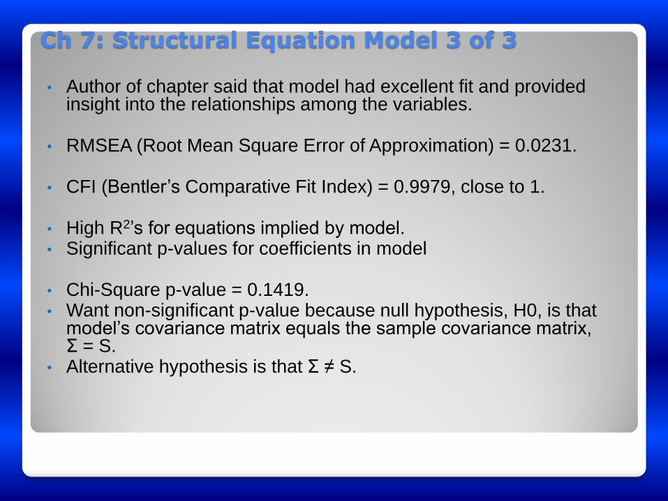
• Author of chapter said that model had excellent fit and provided insight into the relationships among the variables.
• RMSEA (Root Mean Square Error of Approximation) = 0.0231.
• CFI (Bentler’s Comparative Fit Index) = 0.9979, close to 1.
• High R2’s for equations implied by model. • Significant p-values for coefficients in model
• Chi-Square p-value = 0.1419. • Want non-significant p-value because null hypothesis, H0, is that
model’s covariance matrix equals the sample covariance matrix, Σ = S.
• Alternative hypothesis is that Σ ≠ S.

Ch 8: Latent Growth Curve 1/4
• Population average slope and intercept . • Y=outcome, T=Time, i=subect index, ε = error.. • Yi = α + βti + εi. Growth pattern over time is assumed to be linear.
• Random effects allow estimation of individual growth curve for each
subject. • Yi = αi + βiti + εi.
• If 5 timepoints, estimate for subject i at time 1 is Y1i = αi. • At time 2, Y2i = αi + βi; at time 5, Y5i = αi + 4βi.
• In SEM, factors A and B function as the random intercept and slope.
Y1 Y2 Y3 Y4 Y5
F_α F_β 1
1
1
1
1
0
1 2
3 4
ε1 ε2 ε3 ε4 ε5

Ch 8: Latent Growth Curve 2/4
• Equations for latent growth curve, in terms of factors • Y1i = F_αi + εi, Y2i = F_αi + F_βiti + εi; Y3i = F_αi + 2F_βiti + εi,
• Y4i = F_αi + 3F_βiti + εi, Y5i = F_αi + 4F_βiti + εi.
• Proc Mixed or Proc CALIS? • Dataset, Growth contains ID, Y1-Y5.
• ods html newfile=proc path="c:\tempfiles"; ods graphics on; • proc calis method=ml data=growth plots=residuals; • lineqs • y1 = 0. * Intercept + f_alpha + e1, • y2 = 0. * Intercept + f_alpha + 1 * f_beta + e2, • y3 = 0. * Intercept + f_alpha + 2 * f_beta + e3, • y4 = 0. * Intercept + f_alpha + 3 * f_beta + e4, • y5 = 0. * Intercept + f_alpha + 4 * f_beta + e5; • • mean f_alpha f_beta; • run; ods graphics off; ods html close;

Ch 8: Latent Growth Curve 3/4
• *** Proc Mixed Fixed Slope and Intercept ***; • ods html newfile=proc path="c:\tempfiles"; ods graphics on; • Proc Mixed Data=LongGrow Method=REML NOCLPRINT; • Class ID; • Model Y=TimeB/ Solution Influence(effect=ID Est); • Repeated / Type=UN Subject=ID R RCorr; • Run; • ods graphics off; ods html close;
• *** Proc Mixed Random Slope and Intercept ***; • ods html newfile=proc path="c:\tempfiles"; ods graphics on; • Proc Mixed Data=LongGrow Method=REML NOCLPRINT; • Class ID; • Model Y=TimeB/ Solution Influence(effect=ID Est); • Random Int TimeB / type=un sub=id solution; • Run; • ods graphics off; ods html close;
Ch 8: Latent Growth Curve 4/4
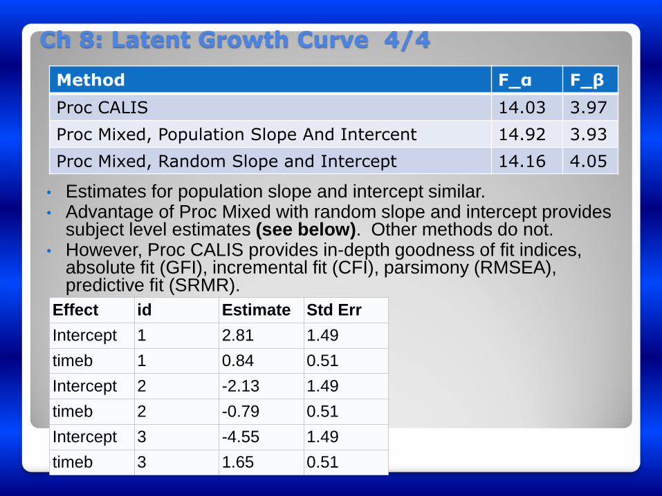
• Estimates for population slope and intercept similar. • Advantage of Proc Mixed with random slope and intercept provides
subject level estimates (see below). Other methods do not. • However, Proc CALIS provides in-depth goodness of fit indices,
absolute fit (GFI), incremental fit (CFI), parsimony (RMSEA), predictive fit (SRMR).
Method F_α F_β
Proc CALIS 14.03 3.97
Proc Mixed, Population Slope And Intercent 14.92 3.93
Proc Mixed, Random Slope and Intercept 14.16 4.05
Effect id Estimate Std Err
Intercept 1 2.81 1.49
timeb 1 0.84 0.51
Intercept 2 -2.13 1.49
timeb 2 -0.79 0.51
Intercept 3 -4.55 1.49
timeb 3 1.65 0.51

Conclusions – Book Worth Reading
Useful reference book for how to set up structural equation models with a graphical user interface for single group analysis.
Helpful tool in seeing how Proc CALIS code is generated from a structural equation model diagram.
Easy-to-follow examples of Proc CALIS.
Shows how to set covariances to zero, how to set paths to constants, and how to add intercepts.
Not a self-teaching book on SEM; need to learn SEM theory through other books or courses.

Contact
Brandy R. Sinco
Statistician and Programmer Analyist
University of Michigan School of Social Work
1080 S. University St.
Ann Arbor, MI 48109-1106
734-763-7784
E-Mail: [email protected]