1

HST.582J/6.555J/16.456JGari D. Clifford

gari [at] mit . eduhttp://www.mit.edu/~gari

© G. D. Clifford 2005-2009

Blind Source Separation:PCA & ICA

What is BSS?Assume an observation (signal) is a linear mix of >1 unknown independent source signals

The mixing (not the signals) is stationary

We have as many observations as unknown sources

To find sources in observations- need to define a suitable measure of independence

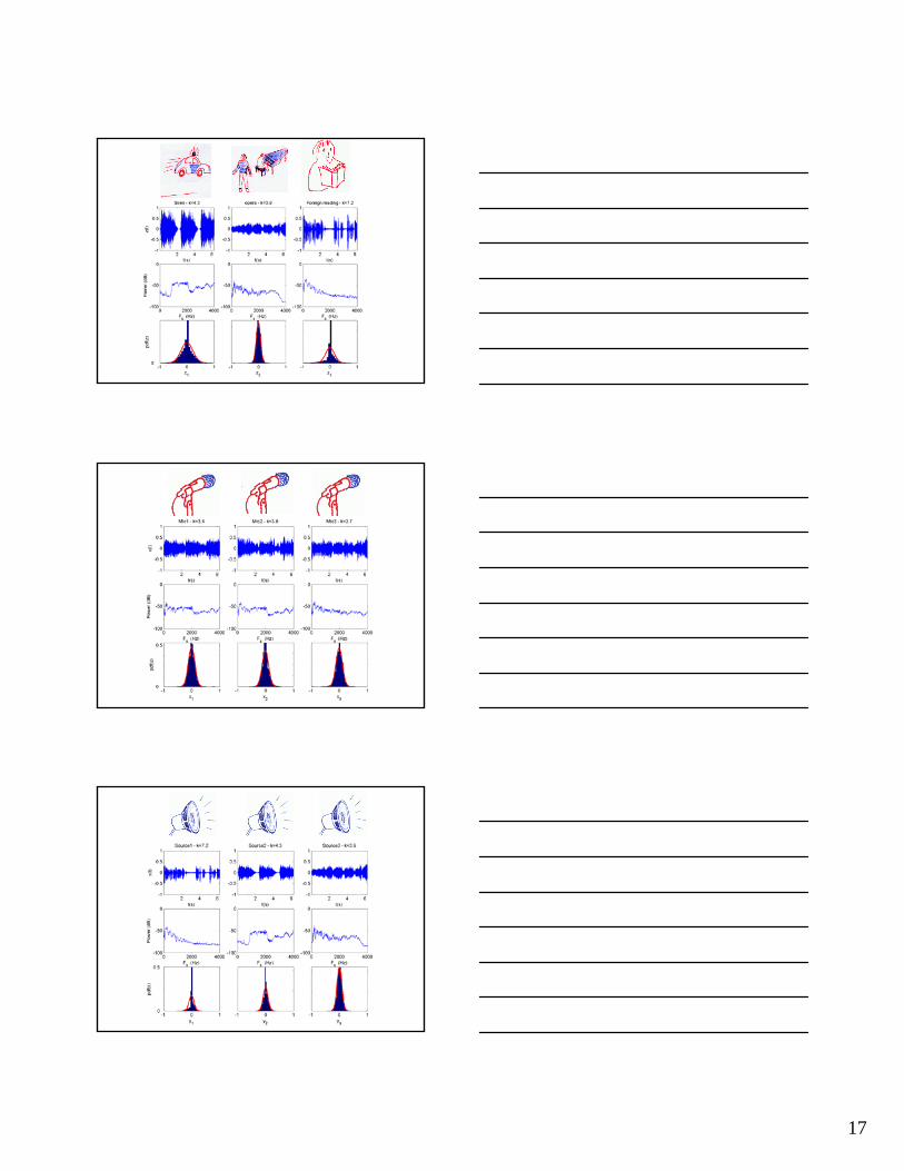
… For example - the cocktail party problem (sources are speakers and background noise):

The cocktail party problem - find Z

A

z1

z2

zN

XTZT

XT=AZT

x1

x2

xN

2

Formal statement of problem

• N independent sources … Zmn ( M xN )

• linear square mixing … Ann ( N xN ) (#sources=#sensors)

• produces a set of observations … Xmn ( M xN )….. XT = AZT

Formal statement of solution• ‘demix’ observations … XT ( N xM )

into YT = WXT

YT ( NxM ) ≈ ZT W ( N xN ) ≈ A-1

How do we recover the independent sources? ( We are trying to estimate W ≈ A-1 )

…. We require a measure of independence!

‘Signal’ source

‘Noise’ sources

Observed mixtures

ZT XT=AZT YT=WXT

3

XT = A ZT

YT = W XT

TT

T T

The Fourier Transform

(Independence between components is assumed)

Recap: Non-causal Wiener filtering

x[n] - observation

y[n] - ideal signal

d[n] - noise component

Ideal Signal Sy(f )

Noise Power Sd(f )

Observation Sx(f )

Filtered signal: Sfilt (f ) = Sx(f ).H(f )

f

4

BSS is a transform?• Like Fourier, we decompose into components by

transforming the observations into another vector space which maximises the separation between interesting (signal) and unwanted (noise).

• Unlike Fourier, separation is not based on frequency-It’s based on independence

• Sources can have the same frequency content

• No assumptions about the signals (other than they are independent and linearly mixed)

• So you can filter/separate in-band noise/signals with BSS

Principal Component Analysis

• Second order decorrelation = independence

• Find a set of orthogonal axes in the data (independence metric = variance)

• Project data onto these axes to decorrelate

• Independence is forced onto the data through the orthogonality of axes

• Conventional noise / signal separation technique

Singular Value DecompositionDecompose observation X=AZ into….

X=USVT

• S is a diagonal matrix of singular values with elements arranged in descending order of magnitude (the singular spectrum)

• The columns of V are the eigenvectors of C=XTX(the orthogonal subspace … dot(vi,vj)=0 ) … they ‘demix’ or rotate the data

• U is the matrix of projections of X onto the eigenvectors of C … the ‘source’ estimates

5

Singular Value DecompositionDecompose observation X=AZ into….

X=USVT

Eigenspectrum of decomposition• S = singular matrix … zeros except on the leading diagonal • Sij (i=j) are the eigenvalues½

• Placed in order of descending magnitude• Correspond to the magnitude of projected data along each eigenvector• Eigenvectors are the axes of maximal variation in the data

Variance = power (analogous to Fourier

components in power spectra)

[stem(diag(S).^2)] Eigenspectrum=Plot of eigenvalues

SVD: Method for PCA

6

SVD noise/signal separationTo perform SVD filtering of a signal, use a truncated SVD

decomposition (using the first p eigenvectors)

Y=USpVT

[Reduce the dimensionality of the data by discarding noise projections Snoise=0Then reconstruct the data with just the signal subsapce]

Most of the signal is contained in the first few principal components.

Discarding these and projecting back into the original observation space effects a noise-filtering or a noise/signal separation

Real dataX

Xp =USpVT

S2

Xp … p=2

λ n

Xp … p=4

Two dimensional example

7

Independent Component AnalysisAs in PCA, we are looking for N different vectors onto which we can project our observations to give a set of N maximally independent signals (sources)

output data (discovered sources) dimensionality = dimensionality of observations

Instead of using variance as our independence measure (i.e. decorrelating) as we do in PCA, we use a measure of how statistically independent the sources are.

8

ICA: The basic idea ...

Assume underlying source signals (Z ) are independent.

Assume a linear mixing matrix (A )… XT=AZT

in order to find Y (≈Z ), find W, (≈A-1 ) ...

YT=WXT

How? Initialise W & iteratively update W to minimise or maximise a cost function that measures the (statistical) independence between the columns of the YT.

Non-Gaussianity ⇒ statistical independence?From the Central Limit Theorem, - add enough independent signals together, Gaussian PDF

Sources, Z

P(Z) (subGaussian)

Mixtures (XT=AZT)

P(X) (Gaussian)

Recap: Moments of a distribution

9

Higher order moments (3rd -skewness)

μx

Higher order moments (4th-kurtosis)

μx

SuperGaussianSubGaussian

Gaussians are mesokurtic with κ =3

Non-Gaussianity ⇒ statistical independence?Central Limit Theorem: add enough independent signals together,

Gaussian PDF ∴ make data components non-Gaussian to find independent sources

Sources, Z

P(Z) (κ <3 (1.8) )

Mixtures (XT=AZT)

P(X) (κ =3.4)

(κ =3)

10

Recall – trying to estimate W

Assume underlying source signals (Z ) are independent.

Assume a linear mixing matrix (A )… XT=AZT

in order to find Y (≈Z ), find W, (≈A-1 ) ...

YT=WXT

Initialise W & iteratively update W with gradient descent to maximise kurtosis.

Gradient descent to find W• Given a cost function, ξ , we update each

element of W ( ) at each step, τ ,

• … and recalculate cost function• (η is the learning rate (~ 0.1), and speeds up

convergence.)

wij

W=[1 3; -2 -1]

Iterations

wij

κ 10

5

Weight updates to find:(Gradient ascent)

11

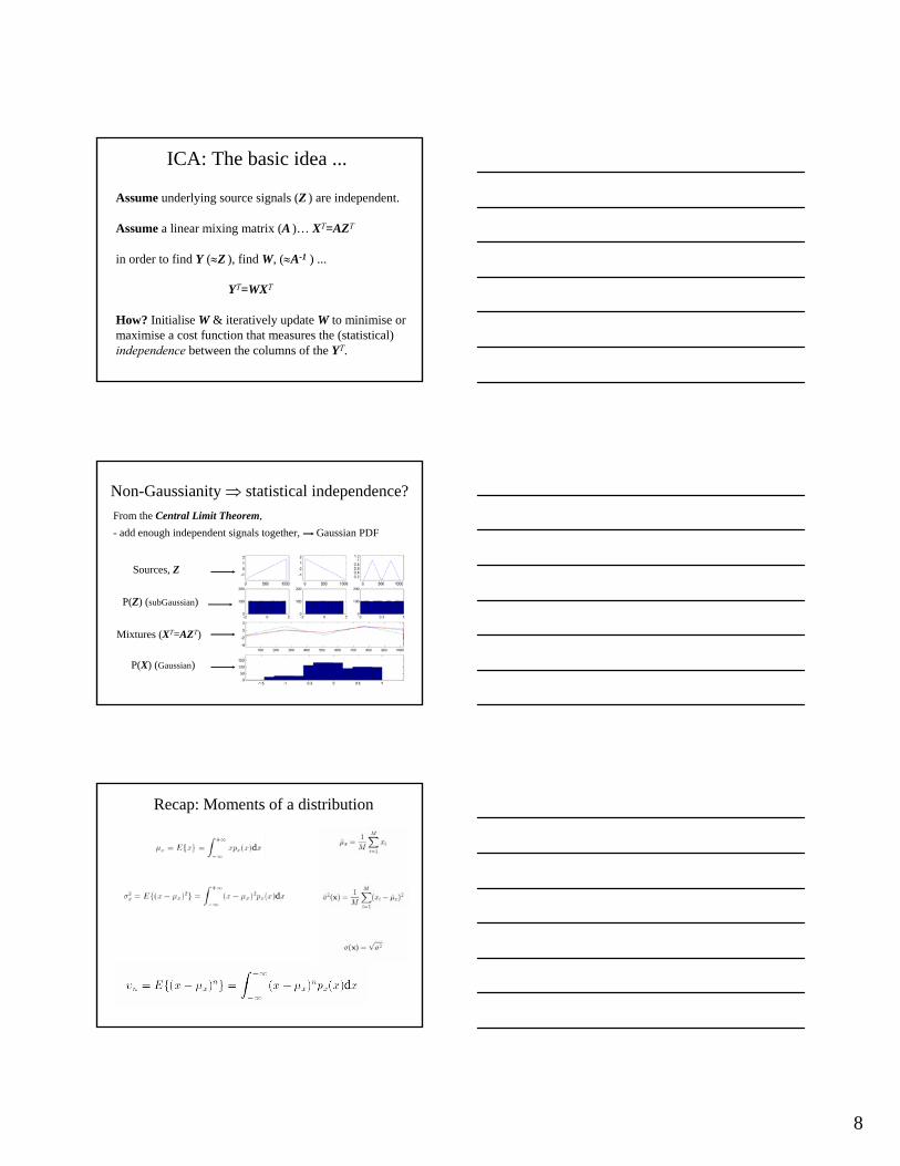
Gradient descent

min (1/|κ1|, 1/|κ2|) | κ = max

Gradient Descent

ξ = min (1/|κ1|, 1/|κ2|) | κ = max

• Cost function, ξ , can be maximum κ or minimum 1/κ

Gradient descent example

• Imagine a 2-channel ECG, comprised of two sources;– Cardiac – Noise

… and SNR=1 X1

X2

12

Iteratively update W and measure κ

Y1

Y2

Iteratively update W and measure κ

Y1

Y2

Iteratively update W and measure κ

Y1

Y2

14

Iteratively update W and measure κ

Y1

Y2

Iteratively update W and measure κ

Y1

Y2

Maximized κ for non-Gaussian signal

Y1

Y2

15

Outlier insensitive ICA cost functions

In general we require a measure of statistical independence which we maximise between each of the N components.

Non-Gaussianity is one approximation, but sensitive to small changes in the distribution tail.

Other measures include:

Measures of statistical independence

• Mutual Information II,

• Entropy (Negentropy, JJ )… and

• Maximum (Log) Likelihood (Note: all are related to κ )

Entropy-based cost functionKurtosis is highly sensitive to small changes in distribution tails. A more robust measures of Gaussianity is based on differential entropy H(y),

… negentropy:

where ygauss is a Gaussian variable with the same covariance matrix as y. J(y) can be estimated from kurtosis …

Entropy: measure of randomness- Gaussians are maximally random

16

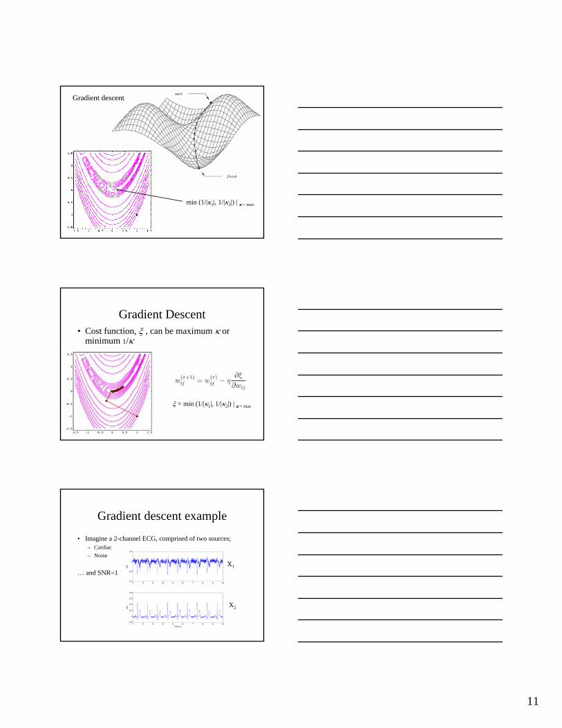
Minimising Mutual InformationMutual information (MI) between two vectors x and y :

always non-negative and zero if variables are independent …therefore we want to minimise MI.

MI can be re-written in terms of negentropy …

where c is a constant. … differs from negentropy by a constant and a sign change

II = Hx + Hy - Hxy

Generative latent variable modelling N observables, X ... from N sources, zi through a linear mapping W=wij

Latent variables assumed to be independently distributed

Find elements of W by gradient ascent - iterative update by

where is some learning rate (const) … andis our objective cost function, the log likelihood

Independent source discovery using Maximum Likelihood

… some real examples using ICA

The cocktail party problem revisited

17

18

Why? … In XT=AZT, insert a permutation matrix B …

XT=ABB-1ZT ⇒ B-1ZT … = sources with different col. order.

⇒ sources change by a scaling A AB

… ICA solutions are order and scale independent because κ is dimensionless

ObservationsSeparation of mixed observations into source estimates is excellent … apart from:

• Order of sources has changed• Signals have been scaled

Separation of sources in the ECG

ζ=3 κ =11 ζ=0 κ =3 ζ=1 κ =5 ζ=0 κ =1.5

19

Transformation inversion for filtering

• Problem - can never know if sources are really reflective of the actual source generators - no gold standard

• De-mixing might alter the clinical relevance of the ECG features

• Solution: Identify unwanted sources, set corresponding (p) columns in W-1 to zero (Wp

-1 ), then multiply back through to remove ‘noise’sources and transform back into original observation space.

Transformation inversion for filtering

Real data

X

Y=WX Z

Xfilt =Wp

-1Y

20

ICA results 4X

Y=WX Z

Xfilt =Wp

-1Y

• PCA is good for Gaussian noise separation• ICA is good for non-Gaussian ‘noise’ separation• PCs have obvious meaning - highest energy components• ICA - derived sources : arbitrary scaling/inversion & ordering

…. need energy-independent heuristic to identify signals / noise• Order of ICs change - IC space is derived from the data.

- PC space only changes if SNR changes.• ICA assumes linear mixing matrix • ICA assumes stationary mixing• De-mixing performance is function of lead position• ICA requires as many sensors (ECG leads) as sources• Filtering - discard certain dimensions then invert transformation• In-band noise can be removed - unlike Fourier!

Summary

Fetal ECG lab preparation

21

Fetal abdominal recordings

• Maternal ECG is much larger in amplitude • Maternal and fetal ECG overlap in time domain• Maternal features are broader, but• Fetal ECG is in-band of maternal ECG

(they overlap in freq domain)• 5 second window … Maternal HR=72 bpm / Fetal HR = 156bpm

Maternal QRS

Fetal QRS

MECG & FECG spectral propertiesFetal QRS power region

ECG EnvelopeMovement ArtifactQRS ComplexP & T WavesMuscle NoiseBaseline Wander

Fetal /Maternal Mixture

Maternal

Noise

Fetal