1

Blind Joint MIMO ChannelEstimation and Decoding

Thomas R. Dean, Member, IEEE, Mary Wootters, Member, IEEE, and Andrea J. Goldsmith, Fellow, IEEE

Abstract—We propose a method for MIMO decoding whenchannel state information (CSI) is unknown to both the transmit-ter and receiver. The proposed method requires some structurein the transmitted signal for the decoding to be effective,in particular that the underlying sources are drawn from ahypercubic space. Our proposed technique fits a minimumvolume parallelepiped to the received samples. This problemcan be expressed as a non-convex optimization problem thatcan be solved with high probability by gradient descent. Ourblind decoding algorithm can be used when communicating overunknown MIMO wireless channels using either BPSK or MPAMmodulation. We apply our technique to jointly estimate MIMOchannel gain matrices and decode the underlying transmissionswith only knowledge of the transmitted constellation and withoutthe use of pilot symbols. Our results provide theoretical guar-antees that the proposed algorithm is correct when applied tosmall MIMO systems. Empirical results show small sample sizerequirements, making this algorithm suitable for realisticallyencountered block-fading channels. Our approach has a lossof less than 3dB compared to zero-forcing with perfect CSI,imposing a similar performance penalty as space-time codingtechniques without the loss of rate incurred by those techniques.

Index Terms—MIMO, Multiuser detection, Blind source sep-aration, Optimization

I. INTRODUCTION

In this work we propose a method to blindly estimate MIMOchannels and decode the underlying transmissions. Given onlyknowledge of the statistics of the channel gain matrix, theconstellation, and the channel noise, we exploit the geometryof the constellation in order to jointly estimate the channelgain matrix and decode the underlying data. More precisely,we exploit the fact that the underlying constellation is oftenhypercubic, i.e. forms a regular n-dimensional polytope withmutually perpendicular sides, as is the case with BPSK orMPAM modulation. The technique presented in this work canalso be applied to decoding and estimation in the SIMO MAC,where channel gains are unknown at the receiver and there isno coordination among transmitters.

In modern cellular systems, there is up to 15% transmissionoverhead dedicated to performing channel estimation [1]. Im-proving channel estimation techniques, through, for example,

T. Dean is with the Department of Electrical Engineering, Stanford, CA94305 USA (e-mail: trdean@stanford.edu).

M. Wootters is with the Department of Computer Science and theDepartment of Electrical Engineering, Stanford, CA 94305 USA (e-mail:marykw@stanford.edu).

A. Goldsmith is with the Department of Electrical Engineering, Stanford,CA 94305 USA (email: andrea@ee.stanford.edu).

This work was presented in part in 2017 at IEEE Globecom in Singapore.T. Dean is supported by the Fannie and John Hertz Foundation. This workwas supported in part by the NSF Center for Science of Information underGrant CCF-0939370

sparse dictionary learning [2], is an active area of research.In practice, channel state information (CSI) is not alwaysneeded to decode, but schemes that communicate withoutCSI impose losses in rate or increased symbol error rates[3]. Additionally, blind decoding schemes for MIMO systemsexist, but they are often inefficient in terms of complexityor sample size requirements. This is discussed in more detailin Section II. Obtaining accurate channel estimates is likelyto become more challenging in future generation wirelesssystems, which will likely have both increased spatial diversityand decreased coherence times [4]. Hence, improvements tochannel estimation, or to schemes that communicate withoutCSI, have the potential to reduce overhead as well as improveperformance in current and future wireless systems.

This work is also motived by research in physical-layersecurity. Several works have proposed keyless authenticationschemes that attempt to identify users based on properties ofthe physical channel over which they communicate (see, forexample [5], or [6] for a survey). Since MIMO channels areoften well conditioned, and hence invertible, such schemesrequire that CSI remains hidden from an adversary. Our workshows that MIMO systems inherently leak CSI when theunderlying source is structured. From a security perspective,this work implies that an eavesdropper need not have knowl-edge of pilot symbols nor any knowledge of the data beingtransmitted in order to efficiently intercept and decode MIMOcommunications. Any scheme that attempts to provide securityby hiding or obscuring pilot symbols will be insecure.

The blind decoding technique introduced in our work is mo-tivated by a classical problem in convex optimization: fittinga minimum volume ellipsoid (also known as the Lowner-Johnellipsoid) to a set of samples, as given in [7]. The methodproposed in this work fits samples to within a parallelepiped,i.e. an n-dimensional polytope that has parallel and congruentopposite faces, thereby recovering the inverse of the channelgain matrix. In this work, we focus on MIMO systems thathave a small number of transmit antennas, specifically up to 8;this choice of parameters captures nearly all MIMO systemsin use in real-world wireless systems today, for example see[8] or [9].

We outline the major contributions of this work as follows:• We introduce a novel (non-convex) optimization problem,

whose solutions capture those of the blind decodingproblem. Our formulation exploits the structure of theunderlying constellation so that solving this optimizationproblem both estimates the channel gain matrix anddetects the underlying data symbols using far fewer sam-ples of received symbols than previous blind decoding

2

techniques.• Despite the fact that this problem is non-convex, we

give both theoretical and empirical results showing thatgradient descent is effective for solving the blind MIMOdecoding problem. More precisely, for general values ofn, we derive sufficient conditions to ensure that globaloptima correspond to solutions of the blind decodingproblem for the case where BPSK is transmitted andin the limit of infinite SNR. We further relate the blinddecoding problem to the Hadamard Maximal Determinantproblem. For n ≤ 4, we present necessary conditions sothat there are no spurious optima within the domain ofthe optimization problem, implying that our approach willalways return a solution to the blind decoding problem.Further, we provide evidence that formulating equivalentnecessary conditions for larger values of n is likelyintractable.

• For n ≤ 4, we give theoretical results that relate thenumber of observed samples to the probability that ourmethod returns a correct solution to the blind decodingproblem. Our theoretical results nearly exactly match ourempirical results. Notice that n ≤ 4 captures the majorityof MIMO systems in use today.

• Although it seems difficult to provide theoretical evidencethat gradient descent performs well for large values of n,we present empirical evidence suggesting that gradientdescent efficiently solves our non-convex optimizationproblem and the blind decoding problem for values ofn as high as n = 15 and for values of M as large asM = 16. Further, our empirical evidence shows that ourapproach is robust in the presence of AWGN and thatdecoding performance is comparable to known methodsthat communicate over a MIMO channel without CSIor with imperfect CSI. In particular, our blind methodoutperforms existing non-blind methods when the CSI issomewhat inaccurate.

The remainder of the paper is organized as follows. In Sec-tion II we provide a survey of techniques related to our work.Section III describes our system model. Section IV outlines theoptimization problem that solves the blind decoding problem,as well as algorithms that solve this optimization problem;the theoretical performance of these algorithms is shown inSection V. Section VI presents empirical results that supportthe theory contained in Section V. Concluding remarks areprovided in Section VII. Proofs not contained in Section Vare found in the appendices.

II. RELATED WORK

The problem of joint blind channel estimation and decodingis not new. For example, in [10], the authors apply MMSEtechniques to the blind decoding of MIMO problems oversmall alphabets while simultaneously recovering the under-lying channel gain matrix. The approach in [10] requires thenumber of samples of received signals used by the algorithmto grow linearly with constellation size, which is exponentialin n, the number of transmit antennas. The approach in [10]only requires the underlying constellation to be discrete; how-ever, for constellations that are also hypercubic, our approach

requires far fewer received samples than the approach of [10]based on our simulation results.

In addition, blind decoding algorithms have previously beenapplied to hypercubic sources. In [11], the authors present astatistical learning algorithm that applies a modified version ofthe Gram-Schmidt algorithm to an estimate of the covariancematrix of the received signals to learn the channel gain matrix.In a different setting, the authors in [12] learn a parallelepipedfrom a covariance matrix by first orthogonalizing and thenrecovering the rotation through higher order statistics. Ourmethod does not rely on the covariance matrix estimation andour empirical results show that it requires fewer samples thanthe techniques of [11] and [12], especially when the channelgain matrix has a high condition number.

Blind source separation is the separation of a set of unknownsignals that are mixed through an unknown (typically linear)process with no or little information about the mixing processor the source signals. Several previous works have consid-ered using blind source separation techniques for detectionof signals transmitted over unknown MIMO channels. Blindsource separation is typically accomplished through techniquessuch as Principle Component Analysis (PCA), IndependentComponent Analysis (ICA), or Non-Negative Matrix Factor-ization (NMF); see [13] for a survey of these techniques.Other techniques exploit structure in the mixing process, forexample, [14] requires the mixing process to be a Toeplitzmatrix. Our technique differs from traditional blind sourceseparation as we obtain an estimate of the source signals bylearning the inverse of the mixing process rather than directlyestimating the source signals. As an output, our algorithmproduces both an estimate of the mixing process, i.e. thechannel gain matrix, and the source signal, i.e. the transmittedsymbols. Similarly, blind channel estimation techniques havebeen studied, although most commonly for SISO channels.See [15] or [16] for surveys on this topic. The approachpresented in this paper can be viewed outside the context ofcommunicating over an unknown MIMO channel as a generaltechnique that performs blind source separation of sourcesmixed through an unknown, linear process.

Many techniques exist for communications over unknownMIMO channels that do not rely on channel estimation. Forexample, Space-Time Block Coding (STBC) was introducedby Alamouti in [17] and formalized by Tarokh et al. in [3].These techniques rely on coding transmissions using sets ofhighly orthogonal codes so that the receiver can recover thetransmission without CSI. For the case of two transmitters,rate one space-time block codes exist that impose a 3 dBpenalty in terms of SNR at the receiver. For larger numbers oftransmitters, rate one codes do not exist. Our techniques do notrequire any coding at the transmitter and thus do not imposeany rate penalty. Numerical simulation shows the decodingperformance of our technique to be comparable to rate oneSTBC methods.

III. SYSTEM MODEL AND NOTATION

This work focuses on an n× n real-valued MIMO channelwith block fading and AWGN. In Section IV-C, we discuss

3

how this work can be extended to complex-valued channelsand channels with more receivers than transmitters. The input-output relation of this channel is characterized by:

y = Ax + e, (1)

where x is drawn from a standard M -PAM or BPSK constel-lation; that is, Xn for X = 2i − 1 −M : i = 1, 2, . . . ,Mor −1,+1 respectively. The channel matrix A ∈ Rn×n

is drawn from a random distribution. For the simulations inSection VI, we take A to be drawn with i.i.d. entries fromN (0, 1); however, our approach only requires A to be full rankand thus A can be considered to be drawn from an arbitrarydistribution or entirely deterministic. The noise e ∈ Rn hasi.i.d. entries drawn from N (0, σ2). We assume that A is block-fading, meaning that the value of A remains constant for somecoherence time, Tc, after which A is redrawn.

The receiver sees samples y1, . . . ,yk, as in (1). We assumethat the receiver knows the constellation Xn but has noknowledge of the points drawn from it, nor does it have anyknowledge of the matrix A.

Given messages x1, . . . ,xk ∈ Rn, we denote by X then × k-dimensional matrix formed by taking each symbol asa column, and by Y the corresponding matrix with receivedsymbols as columns. Notice that we cannot hope to recoverA,X exactly. Indeed, since the constellation is invariant undersign flips and permutations, we can always write AX =ATT−1X, where T is the product of a permutation matrixand a diagonal matrix with entries ±1, and there is no way todistinguish between the solutions (A,X) and (AT,T−1X).Such a matrix T is termed an admissible transform matrix(ATM) in [10]. Thus, in this work, we aim to recover AT forsome ATM T.

While inevitable, these sign and permutation ambiguitiesdo not pose a huge problem in practice, and we ignore themwhen comparing the results to MIMO decoding algorithmswith known CSI. We justify this approach as follows. First, inthe non-blind estimation case (i.e. where we have some controlover the transmission scheme and allow the transmitter to sendpilot symbols), assuming M > n, the permutation ambiguitycould be resolved by a single pilot symbol. Additionally, if weconsider the SIMO Multiple Access Channel, we can ignorethe issue of permutations of the received signals, for exampleby assuming that identification occurs at a higher protocollayer. Finally, we note that the sign ambiguity can easily beresolved through differential modulation. In practice, it mayalso be possible to resolve these ambiguities by examiningstructure in the transmission scheme, present from eitherprotocol/framing data or structure in the underlying data. Thiscould prove to be difficult, however, if the data is encryptedor compressed, or the underlying transmission protocol isdesigned to thwart such analysis.

The notation bAe rounds elements of A to the nearestelement of X , and κ(A) denotes the condition number ofthe matrix A, which is the ratio of the largest to the smallestsingular value of A. ai denotes a column vector formed fromthe ith column of A and a(j) denotes a row vector formedfrom the jth row of A. We define

[nk

]q

to be the Gaussianbinomial coefficient, which for any prime power q, counts

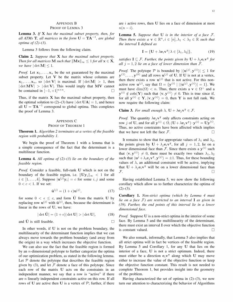
U

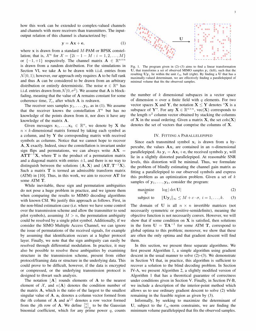
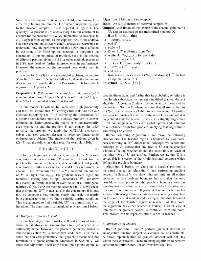
Fig. 1. The program given in (2)–(3) aims to find a linear transformationU, that transforms a set of observed MIMO samples yi (left), such that theresulting Uyi lie within the unit `∞ ball (right). By finding a U that has amaximally-valued determinant, we are effectively finding a parallelepiped ofminimal volume that fits the observed samples.

the number of k dimensional subspaces in a vector spaceof dimension n over a finite field with q elements. For twovector spaces X and Y, the notation X ≤ Y denotes “X is asubspace of Y”. For any X ∈ Rn×n, vec(X) corresponds tothe length n2 column vector obtained by stacking the columnsof X in the usual ordering. Given a matrix X, the set cols(X)denotes the set of vectors that comprise the columns of X.

IV. FITTING A PARALLELEPIPED

Since each transmitted symbol xi is drawn from a hy-percube, the values Axi are contained in an n-dimensionalparallelepiped. As yi = Axi+e, the received symbols yi willlie in a slightly distorted parallelepiped. At reasonable SNRlevels, this distortion will be minimal. Thus, we formulatethe problem of blindly estimating the channel gain matrix asfitting a parallelepiped to our observed symbols and expressthis problem as an optimization problem. Given a set of ksamples of y1, . . . ,yk, consider the program:

maximizeU

log |det U| (2)

subject to ‖Uyi‖∞ ≤M + c · σ, i = 1, . . . , k. (3)

The domain of U is all n × n invertible matrices (notnecessarily symmetric or positive-semidefinite), meaning theobjective function is not necessarily convex. However, we willshow that if some condition on X is satisfied, then solutionsin the form U = TA−1 for some ATM T, correspond toglobal optima to this problem; moreover, we show that theseare often the only optima and that gradient descent will findthem.

In this section, we present three separate algorithms. Wefirst present Algorithm 1, a simple algorithm using gradientdescent in the usual manner to solve (2)–(3). We demonstratein Section VI that, in practice, this algorithm is sufficient torecover a solution to the blind decoding problem. In SectionIV-A, we present Algorithm 2, a slightly modified version ofAlgorithm 1 that has a theoretical guarantee of correctnessunder conditions given in Section V. Finally, in Section IV-B,we include a description of the interior-point method whichallows us to use ordinary gradient descent to solve (2) whileremaining in the feasible region as given by (3).

Informally, by seeking to maximize the determinant ofU, subject to the `∞-norm constraints, we are finding theminimum volume parallelepiped that fits the observed samples.

4

Since U is the inverse of A, up to an ATM, maximizing U iseffectively finding the minimal U−1 which maps the `∞-ballto the observed samples. This is depicted in Figure 1. Thequantity c ·σ present in (3) adds a margin to our constraint toaccount for the presence of AWGN. In practice, values close toc = 3 appear to be optimal as this captures 99% of the additiveGaussian channel noise. More careful analysis is warranted tounderstand how the performance of this algorithm is affectedby the value of c. More optimal methods of margining theconstraints of our optimization problem, such as the methodof ellipsoid peeling, given in [18], or other methods presentedin [19], may lead to further improvements in performance.However, the simple margin presented here works well inpractice.

In order for (2)–(3) to be a meaningful problem, we requireY to be full rank. If Y is not full rank, then the maximumdoes not exist, formally shown in Proposition 1 below, whichis proven in Appendix A.

Proposition 1. If the matrix Y is not full rank, then (2)–(3)is unbounded above. Conversely, if Y is full rank and k ≥ n,then (2)–(3) is bounded above and feasible.

In our model, Y will be full rank with high probabilityand thus, we assume that Y is always full rank and turn ourattention to solving (2)–(3). Maximizing the determinant ofa positive-semidefinite matrix is a classic problem in convexoptimization. Unfortunately, the matrix A is not necessarilyeven symmetric and the problem is not convex. In orderto solve the problem we apply the MATLAB fminconsolver that uses gradient descent to solve non-linear conicoptimization problems. The gradient of the problem given in(2)–(3) has the following value (see, for example, [20]):

∇ (log |det U|) =(U−1

)ᵀ. (4)

Before we begin gradient descent, we check that Y is wellconditioned. As noted above, Y must be full rank for theproblem to make sense; however, if Y is full rank but poorlyconditioned, similar issues will arise and U may not invert thechannel. Thus, we return FAIL if κ(Y), the condition numberof Y, is larger than κmax. The gradient descent algorithmrequires a starting point as input, denoted as U(0). We drawthis matrix uniformly at random over the set of all orthogonalmatrices, O(n), using the method described in [21]. We checkthat this random U(0) in fact satisfies the constraints; if it doesnot, we generate a new random matrix and scale the matrixby a constant term until we find a suitable starting condition.This is guaranteed to find a suitable U(0) in at most log2 κmax

iterations. The algorithm is summarized as Algorithm 1 below.

A. Modified Gradient Descent

In practice, Algorithm 1 works well and empirical resultsshow that it always returns solutions to (2)–(3) when k issufficiently large. However, the problem geometry, which isstudied in Section V, is non-convex and there is in fact asmall but non-zero probability that gradient descent will notterminate at a global optimum. Moreover, in Section V, weshow that Algorithm 1 will only fail to find a global optima at

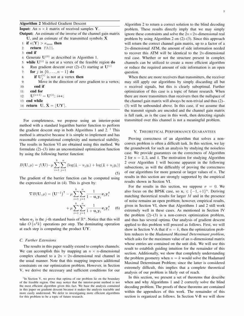
Algorithm 1 Fitting a ParallelepipedInput: An n× k matrix of received samples Y.Output: An estimate of the inverse of the channel gain matrix

U, and an estimate of the transmitted symbols X1: if κ(Y) > κmax then2: return FAIL3: end if4: scale = 1;5: Draw U(0) uniformly from O(n);6: while |U(0)yi|∞ > 1 for any i do7: scale = scale * 2;8: Draw U(0) uniformly from O(n);9: U(0) = U(0) / scale;

10: end while11: Run gradient descent over (2)–(3) starting at U(0) to find

an optimal value of U;12: return U, X = bUYe.

specific dimensions, and further that its probability of failure islow. In this subsection, we present a modified gradient descentalgorithm, Algorithm 2, shown below, which is motivated bythe theory in Section V, where we show that all strict solutionsto (2)–(3) lie on vertices of the problem boundary. Algorithm2 always terminates at a vertex of the feasible region, and it isconjectured that, for general n, when k is slightly larger thann, all non-singular vertices are global optima and solutionsto our channel estimation problem, implying that Algorithm 2will always be correct.

Before describing Algorithm 2, we make the followingobservations. The feasible region is bounded by 2kn halfs-paces, forming an Rn2

dimensional polytope. We denote thispolytope as P . Notice that any row of U can be changedwithout effecting whether or not the constraints on each ofthe other rows of U are satisfied. Further, we say that U is avertex if it is a vertex of the n2-dimensional polytope whichdefines the problem boundary.

Algorithm 2 begins by choosing a starting position inthe same manner as Algorithm 1 and performing gradientdescent. In Section V it is shown that not only are all optimacontained on the problem boundary but also that the onlypossible critical points on the problem boundary exist aslow-dimensional affine subspaces, along which the objectivefunction is constant valued. If gradient descent reaches such asubspace, then Algorithm 2 continues by choosing a directionon this subspace at random and moving in that direction untilthe edge of the feasible region is reached. At this point,the algorithm has either reached a vertex, in which case itterminates, or gradient descent is continued from this point.This process can be repeated until a vertex is reached.

B. Interior-Point Method

Both Algorithms 1 and 2 perform gradient descent onan objective function subject to a convex set of constraints.A naıve implementation of gradient descent will not staywithin these constraints. There are many algorithms to performconstrained optimization, for an overview, see [19].

5

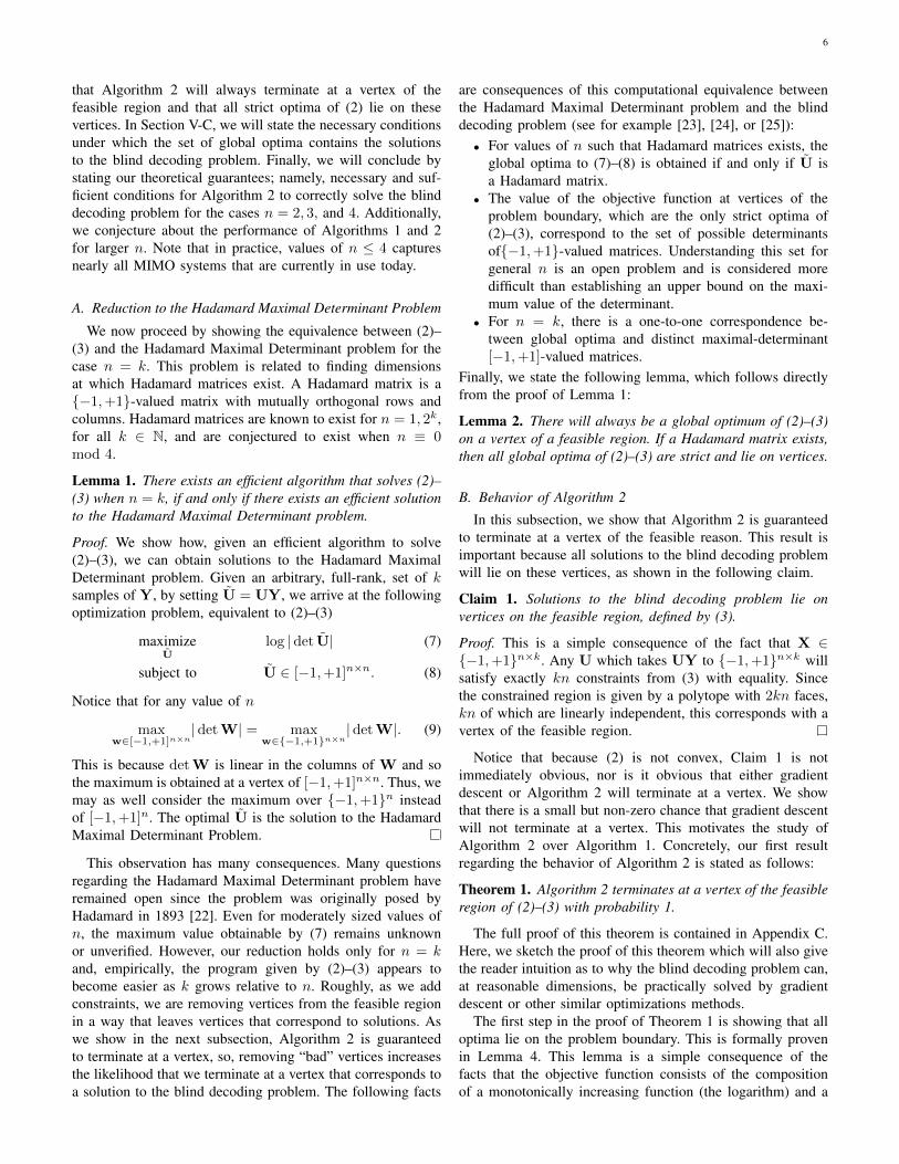
Algorithm 2 Modified Gradient DescentInput: An n× k matrix of received samples Y.Output: An estimate of the inverse of the channel gain matrix

U, and an estimate of the transmitted symbols X1: if κ(Y) > κmax then2: return FAIL3: end if4: Generate U(0) as described in Algorithm 1.5: while U(i) is not at a vertex of the feasible region do6: Run gradient descent over (2)–(3) starting at U(i)

7: for j in 0, . . . , n− 1 do8: if U

(i)j is not at a vertex then

9: Move in the direction of zero gradient to a vertex;10: end if11: end for12: U(i+1) = U(i); i++;13: end while14: return U, X = bUYe.

For completeness, we propose using an interior-pointmethod with a standard logarithm barrier function to performthe gradient descent step in both Algorithms 1 and 2. 1 Thismethod is attractive because it is simple to implement and hasreasonable computational complexity and numerical stability.The results in Section VI are obtained using this method. Weformulate (2)–(3) into an unconstrained optimization functionby using the following barrier function:

B(U, µ) = f(U)−µk∑

i=1

n∑j=1

(log(1− ujyi) + log(1 + ujyi))

(5)The gradient of the barrier function can be computed usingthe expression derived in (4). This is given by:

∇B(U, µ) =(U−1

)ᵀ − µ k∑i=1

n∑j=1

1

1− ujyiejy

ᵀi

+ µ

k∑i=1

n∑j=1

1

1 + ujyiejy

ᵀi (6)

where ej is the j-th standard basis of Rn. Notice that this willtake O

(n2k

)operations per step. The dominating operation

at each step is computing the product UY.

C. Further Extensions

The results in this paper readily extend to complex channels.We can accomplish this by mapping an n × n-dimensionalcomplex channel to a 2n × 2n-dimensional real channel inthe usual manner. Note that this mapping imposes additionalconstraints on our optimization problem. However, in SectionV, we derive the necessary and sufficient conditions for our

1In Section V, we prove that optima of our problem lie on the boundaryof the feasible region. One may notice that the interior-point method is notthe most efficient algorithm given this fact. We base the analysis containedin this paper on gradient descent because it makes the analysis tractable andmore easily understood. We defer to investigating more efficient algorithmsfor this problem to be a topic of future research.

Algorithm 2 to return a correct solution to the blind decodingproblem. These results directly imply that we may simplyignore these constraints and solve the 2n×2n-dimensional realproblem by using Algorithm 2 on (2)–(3). Since this approachwill return the correct channel gain matrix, up to a factor of a2n-dimensional ATM, the amount of side information neededto recover this ATM will be identical to the 2n-dimensionalreal case. Whether or not the structure present in complexchannels can be utilized to create a more efficient algorithmor reduce the required amount of side information is an openquestion.

When there are more receivers than transmitters, the receivermay still apply our algorithms by simply discarding all butn received signals, but this is clearly suboptimal. Furtheroptimization of this case is a topic of future research. Whenthere are more transmitters than receivers then the nullspace ofthe channel gain matrix will always be non-trivial and thus (2)–(3) will be unbounded above. In this case, if we assume thatthe transmit signals are uncoded and the channel gain matrixis full rank, as is the case in this work, then detecting signalstransmitted over this channel is not a meaningful problem.

V. THEORETICAL PERFORMANCE GUARANTEES

Proving correctness of an algorithm that solves a non-convex problem is often a difficult task. In this section, we laythe groundwork for such an analysis by studying the noiselesscase. We provide guarantees on the correctness of Algorithm2 for n = 2, 3, and 4. The motivation for studying Algorithm2 over Algorithm 1 will become apparent in the followingsubsections, as will the difficultly of proving the correctnessof our algorithms for more general or larger values of n. Theresults in this section are strongly supported by the empiricalresults shown in Section VI.

For the results in this section, we suppose σ = 0. Wealso focus on the BPSK case, so xi ∈ −1,+1n. Derivingmatching theoretical results for larger M and in the presenceof noise remains an open problem; however, empirical results,given in Section VI, show that Algorithms 1 and 2 still workextremely well in these cases. As mentioned in Section IVthe problem (2)–(3) is a non-convex optimization problem,and thus has several optima. Our analysis of gradient descentapplied to this problem will proceed as follows. First, we willshow in Section V-A that if n = k, then the optimization prob-lem reduces to the Hadamard Maximal Determinant problem,which asks for the maximum value of an n-dimensional matrixwhose entries are contained on the unit disk. We will use thisresult to establish guiding intuition for the remainder of thissection. Additionally, we show that completely understandingthe problem geometry when n = k would solve the HadamardMaximal Determinant Problem; since the latter is consideredextremely difficult, this implies that a complete theoreticalanalysis of our problem is likely out of reach.

In this section, we present a set of theorems that describewhen and why Algorithms 1 and 2 correctly solve the blinddecoding problem. The proofs of these theorems are containedwithin the appendices of this work. The remainder of thissection is organized as follows. In Section V-B we will show

6

that Algorithm 2 will always terminate at a vertex of thefeasible region and that all strict optima of (2) lie on thesevertices. In Section V-C, we will state the necessary conditionsunder which the set of global optima contains the solutionsto the blind decoding problem. Finally, we will conclude bystating our theoretical guarantees; namely, necessary and suf-ficient conditions for Algorithm 2 to correctly solve the blinddecoding problem for the cases n = 2, 3, and 4. Additionally,we conjecture about the performance of Algorithms 1 and 2for larger n. Note that in practice, values of n ≤ 4 capturesnearly all MIMO systems that are currently in use today.

A. Reduction to the Hadamard Maximal Determinant Problem

We now proceed by showing the equivalence between (2)–(3) and the Hadamard Maximal Determinant problem for thecase n = k. This problem is related to finding dimensionsat which Hadamard matrices exist. A Hadamard matrix is a−1,+1-valued matrix with mutually orthogonal rows andcolumns. Hadamard matrices are known to exist for n = 1, 2k,for all k ∈ N, and are conjectured to exist when n ≡ 0mod 4.

Lemma 1. There exists an efficient algorithm that solves (2)–(3) when n = k, if and only if there exists an efficient solutionto the Hadamard Maximal Determinant problem.

Proof. We show how, given an efficient algorithm to solve(2)–(3), we can obtain solutions to the Hadamard MaximalDeterminant problem. Given an arbitrary, full-rank, set of ksamples of Y, by setting U = UY, we arrive at the followingoptimization problem, equivalent to (2)–(3)

maximizeU

log |det U| (7)

subject to U ∈ [−1,+1]n×n. (8)

Notice that for any value of n

maxw∈[−1,+1]n×n

|det W| = maxw∈−1,+1n×n

|det W|. (9)

This is because det W is linear in the columns of W and sothe maximum is obtained at a vertex of [−1,+1]n×n. Thus, wemay as well consider the maximum over −1,+1n insteadof [−1,+1]n. The optimal U is the solution to the HadamardMaximal Determinant Problem.

This observation has many consequences. Many questionsregarding the Hadamard Maximal Determinant problem haveremained open since the problem was originally posed byHadamard in 1893 [22]. Even for moderately sized values ofn, the maximum value obtainable by (7) remains unknownor unverified. However, our reduction holds only for n = kand, empirically, the program given by (2)–(3) appears tobecome easier as k grows relative to n. Roughly, as we addconstraints, we are removing vertices from the feasible regionin a way that leaves vertices that correspond to solutions. Aswe show in the next subsection, Algorithm 2 is guaranteedto terminate at a vertex, so, removing “bad” vertices increasesthe likelihood that we terminate at a vertex that corresponds toa solution to the blind decoding problem. The following facts

are consequences of this computational equivalence betweenthe Hadamard Maximal Determinant problem and the blinddecoding problem (see for example [23], [24], or [25]):• For values of n such that Hadamard matrices exists, the

global optima to (7)–(8) is obtained if and only if U isa Hadamard matrix.

• The value of the objective function at vertices of theproblem boundary, which are the only strict optima of(2)–(3), correspond to the set of possible determinantsof−1,+1-valued matrices. Understanding this set forgeneral n is an open problem and is considered moredifficult than establishing an upper bound on the maxi-mum value of the determinant.

• For n = k, there is a one-to-one correspondence be-tween global optima and distinct maximal-determinant[−1,+1]-valued matrices.

Finally, we state the following lemma, which follows directlyfrom the proof of Lemma 1:

Lemma 2. There will always be a global optimum of (2)–(3)on a vertex of a feasible region. If a Hadamard matrix exists,then all global optima of (2)–(3) are strict and lie on vertices.

B. Behavior of Algorithm 2

In this subsection, we show that Algorithm 2 is guaranteedto terminate at a vertex of the feasible reason. This result isimportant because all solutions to the blind decoding problemwill lie on these vertices, as shown in the following claim.

Claim 1. Solutions to the blind decoding problem lie onvertices on the feasible region, defined by (3).

Proof. This is a simple consequence of the fact that X ∈−1,+1n×k. Any U which takes UY to −1,+1n×k willsatisfy exactly kn constraints from (3) with equality. Sincethe constrained region is given by a polytope with 2kn faces,kn of which are linearly independent, this corresponds with avertex of the feasible region.

Notice that because (2) is not convex, Claim 1 is notimmediately obvious, nor is it obvious that either gradientdescent or Algorithm 2 will terminate at a vertex. We showthat there is a small but non-zero chance that gradient descentwill not terminate at a vertex. This motivates the study ofAlgorithm 2 over Algorithm 1. Concretely, our first resultregarding the behavior of Algorithm 2 is stated as follows:

Theorem 1. Algorithm 2 terminates at a vertex of the feasibleregion of (2)–(3) with probability 1.

The full proof of this theorem is contained in Appendix C.Here, we sketch the proof of this theorem which will also givethe reader intuition as to why the blind decoding problem can,at reasonable dimensions, be practically solved by gradientdescent or other similar optimizations methods.

The first step in the proof of Theorem 1 is showing that alloptima lie on the problem boundary. This is formally provenin Lemma 4. This lemma is a simple consequence of thefacts that the objective function consists of the compositionof a monotonically increasing function (the logarithm) and a

7

multilinear function (the determinant), and that the problemboundary is convex. These facts imply that, given any pointwithin the feasible region that does not lie on the boundary, wecan always move away from the origin in a way that increasesthe objective function.

We have already established in Lemma 2 that when aHadamard matrix exists, all optima are strict. Conversely,at dimensions where Hadamard matrix do not exist, thenone can find non-strict optima. From Lemma 4, we knowthat these non-strict optima must lie on the boundary of thefeasible region. In Lemma 5 and Corollary 1, we furthercharacterize these non-strict optima to show that if a non-strictoptima exists, then they must be restricted to a linear intervalcontained on a face of the polytope which defines the feasibleregion. We further show that all strict optima, regardless of theexistence of a Hadamard matrix must lie on vertices. We usethese fact together with Lemma 3 to guarantee that Algorithm2 reaches a vertex.

In Lemma 6, we show how far gradient descent (or Al-gorithm 1) will proceed towards a vertex. Notice that theconstraints in (3) act on each row of U independently, andU will be at a vertex of the feasible region when there areexactly n constraints active on each row. In fact, we show inLemma 6 that when gradient descent terminates (meaning wehave reached an optima), each row of U will have at leastn− 1 active constraints per row.

When this occurs, U will be on an edge of the feasibleregion; indeed, there is exactly one line on which U can movewhile staying on the boundary of the feasible region and notaffecting the active constraints. We can further show that theobjective function must be constant along this line. Thus, foreach row with n−1 active constraints, we can simply choose adirection at random and move in this direction until we reach avertex. We are thus guaranteed that Algorithm 2 will terminateat the vertex of the feasible region.

C. Maximal Subset PropertyWe have established that Algorithm 2 always terminates on

a vertex of the feasible region. However, such a point mayeither be a global or local optima to (2)–(3) and may notcorrespond to a solution to the blind decoding problem. Inthis light, we now study when vertices of the feasible regioncorrespond to solutions to the blind decoding problem andunderstanding when, if ever, local optima of (2)–(3) exist. Wefirst derive a sufficient condition for the solutions of the blinddecoding problem to correspond to global optima of (2)–(3).More precisely, we will study the following condition of theset x1, . . . ,xk:

Definition 1. A matrix X ∈ [−1,+1]n×k, and correspondingset cols(X) ⊆ [−1,+1]n, with k ≥ n has the maximal subsetproperty if there is a subset cols(V) ⊆ cols(X) of size n sothat if V ∈ Rn×n is the matrix with elements of cols(V) ascolumns, then

|det V| = maxW∈[−1,+1]n×n

|det W|. (10)

That is, X has the maximal subset property if it containsa subset of columns that, when viewed as a matrix, has

a determinant that is maximal among all [−1,+1]-valuedmatrices (and hence also all −1,+1-valued matrices). Withthis definition, we can now state a sufficient condition forsolutions to our problem to be global optima.

Lemma 3. If X has the maximal subset property, then, forall ATMs T, all matrices in the form U = TA−1 are globaloptima of (2)–(3).

Lemma 3 is proved in Appendix B. For small n, we cancompute the probability that a set of k samples has themaximal subset property; this result is given in Appendix F. InSection VI we show that the empirical success probability ofAlgorithm 1 with k samples exactly matches the probabilitydistribution derived in Appendix F.

It is natural to ask whether the converse of Lemma 3 is true.In fact, for M > 2, an explicit counterexample exists, foundthrough computer simulation, that shows that the maximalsubset property is not a necessary condition. This is importantbecause the probability of finding a maximal subset throughuniform sampling decreases rapidly as M and n grow. Indeed,this agrees with our empirical observations, specifically Table Ifound in Section VI, which show that the increase in k requiredto maintain a constant success probability (assuming uniformsampling) appears less than quadratic in M . Having estab-lished the maximum subset property as a sufficient condition,we now continue our analysis of the geometry of our non-convex optimization problem by considering specific valuesof n.

D. The Cases n = 2 and n = 3

For n = 2 and n = 3, it can easily be checked that allfull-rank matrices in −1,+1n×n have the maximal subsetproperty. In other words, the set of possible values of thedeterminant contains two possible absolute values, 0 and 2n−1.For n = 2, one can verify that ATMs are the only orthogonalmatrices that map elements of this set to other elements ofthis set. Further, since a Hadamard matrix exists at n = 2,all optima are strict and vertices of the feasible region. Thesefacts imply the following theorem.

Theorem 2. For n = 2, Algorithms 1 and 2 are correct (thatis, finds a solution to the blind decoding problem) if and onlyif X has the maximal subset property.

For n = 3, the maximal subset property alone is notsufficient to ensure that Algorithms 1 or 2 succeed. Indeed,for any X ∈ −1,+13×3, there exists a matrix Q such thatQX ∈ [−1,+1]3×3, det Q = ±1 and Q /∈ T . This implies theexistence of spurious optima whenever k = 3. However, thesespurious optima will not exist if k ≥ 4 and X contains at leastone additional distinct column beyond the three required forthe maximal subset property. By a distinct column, we meanthat the ith column of X is distinct if xi 6= ±xj for all j 6= i.Notice that this also implies that all columns of X are pair-wise linearly independent. Further, we note that Algorithm1 is no longer guaranteed to be correct for n = 3 becausen = 3 contains no Hadamard matrix. We now formally statea theorem, proven in Appendix D, regarding the performanceof Algorithm 2.

8

Theorem 3. When n = 3, Algorithm 2 is correct withprobability 1 if and only if k ≥ 4 and there exists a 3×4 matrixV, such that cols(V) ⊆ cols(X), span(v1, . . . ,v4) = R3, andall vectors in V are pair-wise linearly independent.

We now turn our attention to quantifying the probabilitythat the conditions required by Theorems 2 and 3 hold. Letr(n, k) denote the probability that a collection of k vectors inFn2 has rank n (and hence the rank in Rn must also be n),

then the probability of the solver succeeding, given k sampleschosen uniformly at random, is given by:

Pr(Success) = r(n, k). (11)

An explicit formula for r(n, k) is derived in Appendix F.Notice that for n = 2, equation (11) expresses the probabilitythat the set of global optima contains solutions to the blinddecoding problem. For n = 3, since we require the existenceof a fourth distinct vector, we find that the probability, for aset of k samples chosen uniformly, that all global optima willbe solutions to be

Pr(Success) = r(n, k) · (1− 2n−k). (12)

We note that, for n = 3, if a collection of samples containsonly the MSP and not an additional distinct column, then Al-gorithm 2 still has a non-zero probability of finding a solutionto the blind decoding problem as the set of global optimastill contains the set of all solutions. Thus the probability ofsuccess of Algorithm 2, conditioned over a uniform selectionof samples, is bounded between (11) and (12). In Section VIwe compare these distributions to our empirical results.

E. The case n = 4.At dimension n = 4, the problem geometry gets slightly

more complicated. The set of possible values of the determi-nants of −1,+14×4 increases to 0,±8,±16, which meansthat not all non-singular vertices of (3) are global optima to(2)–(3). However, we show that for n = 4, the only optima of(2)–(3) are indeed global optima. Unfortunately, for n = k, notall global optima are solutions to the blind decoding problem.Nonetheless, we are able to show that for n = 4, Algorithms1 and 2 both succeed (and solve the blind decoding problem)with probability 1 under proper input conditions.

Before stating Theorem 4, which is proved in AppendixE, we must also introduce equivalence classes of Hadamardmatrices. We say that two Hadamard matrices H1 and H2 areequivalent if there exists and ATM T such that H1 = T ·H2.This is an equivalence relation, and thus decomposes the setof Hadamard matrices into equivalence classes. For n = 4,there are exactly two equivalence classes, which we denote asH(1)

4 and H(2)4 , that are defined as follows:

H(1)4 =

T

1 1 1 11 1 − −1 − 1 −1 − − 1

,∀T ∈ T , (13)

H(2)4 =

T

− 1 1 11 − 1 11 1 − 11 1 1 −

,∀T ∈ T , (14)

where “−” denotes −1. Notice that all vectors in F42 appear

as column vectors in either H(1)4 or H(2)

4 . We say that a vectorbelongs to an equivalence class if it appears as a column vectorin that equivalence class. We now state our result for the casen = 4, which is proven in Appendix E. Notice that becausea Hadamard matrix exists for n = 4, then by Lemma 2, theonly optima of (2)–(3) are strict and hence gradient descentwill always terminate at a vertex even without the modificationgiven in Algorithm 1.

Theorem 4. When n = 4, Algorithm 1 is correct withprobability 1 if and only if k ≥ 5 and cols(X) contains atleast four linearly independent vectors from H(i)

4 and a fifthvector from H(j)

4 for i 6= j.Algorithm 1 will be correct with probability 0.5 if cols(X)

has only four linearly independent vectors belonging to thesame equivalence class.

Theorem 4 implies that we will always require at least 5samples in order to solve the blind decoding problem. Further,assuming that the source symbols are chosen uniformly at ran-dom, this result allows us to quantify the success probabilityof the blind decoding algorithm. This is done in Appendix E,where we show that the success probability for n = 4 is givenby:

Pr(Success) = r(4, k) · r(3, k)4 · (1− 2n−k). (15)

F. Larger n

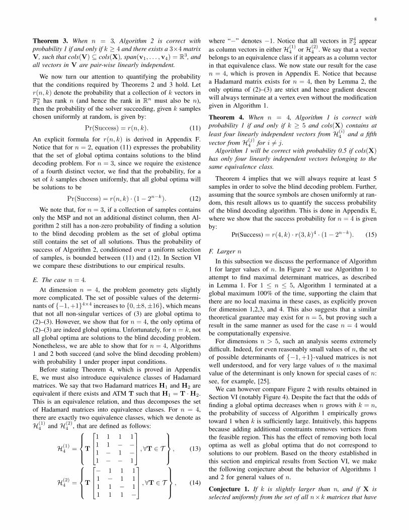
In this subsection we discuss the performance of Algorithm1 for larger values of n. In Figure 2 we use Algorithm 1 toattempt to find maximal determinant matrices, as describedin Lemma 1. For 1 ≤ n ≤ 5, Algorithm 1 terminated at aglobal maximum 100% of the time, supporting the claim thatthere are no local maxima in these cases, as explicitly provenfor dimension 1,2,3, and 4. This also suggests that a similartheoretical guarantee may exist for n = 5, but proving such aresult in the same manner as used for the case n = 4 wouldbe computationally expensive.

For dimensions n > 5, such an analysis seems extremelydifficult. Indeed, for even reasonably small values of n, the setof possible determinants of −1,+1-valued matrices is notwell understood, and for very large values of n the maximalvalue of the determinant is only known for special cases of n:see, for example, [25].

We can however compare Figure 2 with results obtained inSection VI (notably Figure 4). Despite the fact that the odds offinding a global optima decreases when n grows with k = n,the probability of success of Algorithm 1 empirically growstoward 1 when k is sufficiently large. Intuitively, this happensbecause adding additional constraints removes vertices fromthe feasible region. This has the effect of removing both localoptima as well as global optima that do not correspond tosolutions to our problem. Based on the theory established inthis section and empirical results from Section VI, we makethe following conjecture about the behavior of Algorithms 1and 2 for general values of n.

Conjecture 1. If k is slightly larger than n, and if X isselected uniformly from the set of all n×k matrices that have

9

0 2 4 6 8 10 12 14 160

0.1

0.2

0.3

0.4

0.5

0.6

0.7

0.8

0.9

1

n

Succ

ess

Prob

abili

ty

Fig. 2. The probability that Algorithm 2 finds a maximal-determinant matrixwhen used as described in Lemma 4, averaged over 1000 samples. Fordimension at most 5, all optima are global. Above this, we are not guaranteedto find terminate at a maximal matrix. However, as k grows relative to n, theprobability increases again. See Figure 3.

the maximal subset property, then with high probability, theonly optima in (2)–(3) are U = TA−1, for all ATMs T.

VI. EMPIRICAL RESULTS

Having established theoretical results regarding the correct-ness of our algorithm, we now turn our attention to empiricalresults. The simulation results contained in this section areentirely based on Algorithm 1 and demonstrate that Algorithm2 is unnecessary in practice, at least for low dimensions. Theempirical performance of Algorithm 2 does not noticeablyimprove over the performance of Algorithm 1. In order toassess the performance of Algorithm 1, we constructed twosets of experiments. In the first, we ran Algorithm 1 forvarious values of n and M without channel noise in orderto empirically test the conditions under which the solver willreturn the correct solution. In the second, we ran the algorithmusing realistic channel conditions and compared the resultsto the Zero-Forcing and Maximum-Likelihood decoders, bothwith perfect and imperfect CSI.

Table I summarizes the number of samples required forvarious values of n and M so that Algorithm 1 has a 90%probability of returning an optimal solution to (2)–(3). For thevalues of n presented, the success probability is almost entirelyconditioned upon the input value of X rather than randomnessin Algorithm 1; that is, running Algorithm 1 multiple timeson the same X will not improve success rates.

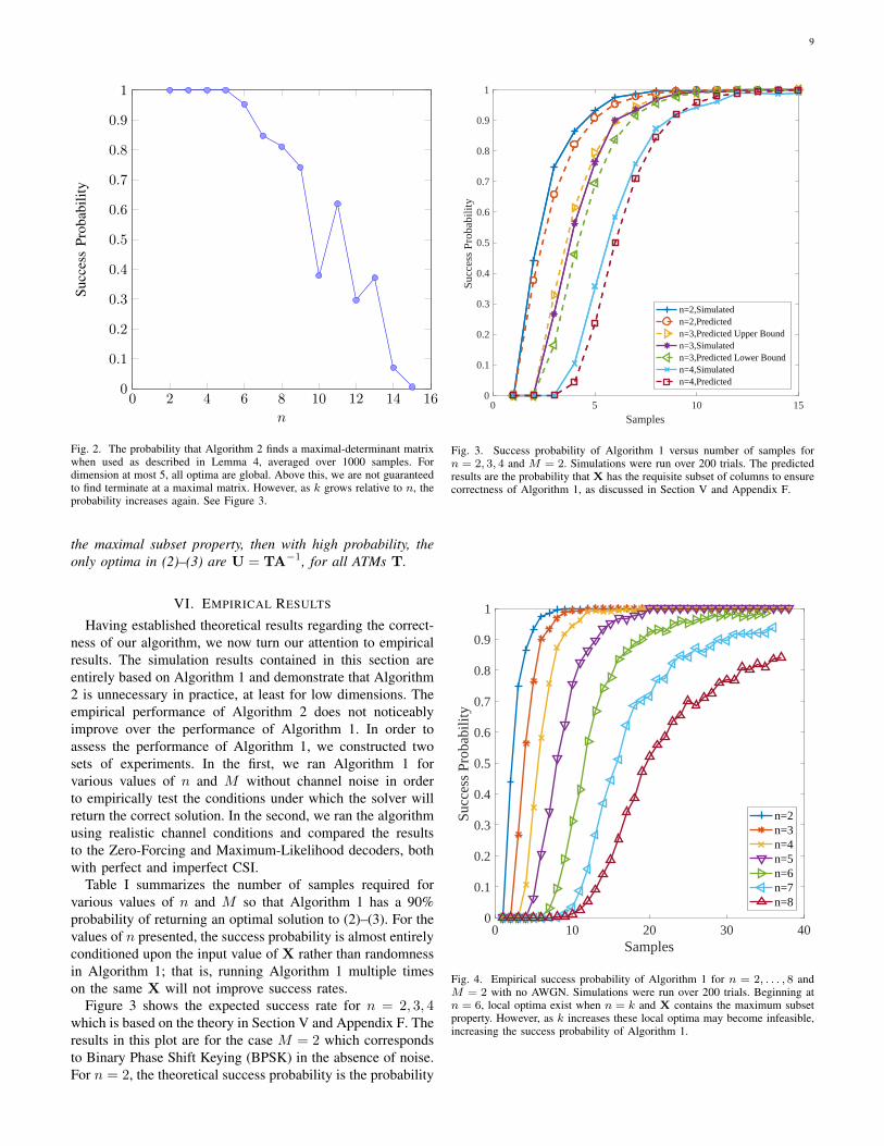
Figure 3 shows the expected success rate for n = 2, 3, 4which is based on the theory in Section V and Appendix F. Theresults in this plot are for the case M = 2 which correspondsto Binary Phase Shift Keying (BPSK) in the absence of noise.For n = 2, the theoretical success probability is the probability

0 5 10 15Samples

0

0.1

0.2

0.3

0.4

0.5

0.6

0.7

0.8

0.9

1

Succ

ess

Prob

abili

ty

n=2,Simulatedn=2,Predictedn=3,Predicted Upper Boundn=3,Simulatedn=3,Predicted Lower Boundn=4,Simulatedn=4,Predicted

Fig. 3. Success probability of Algorithm 1 versus number of samples forn = 2, 3, 4 and M = 2. Simulations were run over 200 trials. The predictedresults are the probability that X has the requisite subset of columns to ensurecorrectness of Algorithm 1, as discussed in Section V and Appendix F.

0 10 20 30 40Samples

0

0.1

0.2

0.3

0.4

0.5

0.6

0.7

0.8

0.9

1

Succ

ess

Prob

abili

ty

n=2n=3n=4n=5n=6n=7n=8

Fig. 4. Empirical success probability of Algorithm 1 for n = 2, . . . , 8 andM = 2 with no AWGN. Simulations were run over 200 trials. Beginning atn = 6, local optima exist when n = k and X contains the maximum subsetproperty. However, as k increases these local optima may become infeasible,increasing the success probability of Algorithm 1.

10

TABLE ISAMPLE SIZE REQUIREMENTS

Algorithm 1n M=2 M=4 M=8 M=162 5 14 29 563 6 23 45 874 10 32 60 1185 14 42 98 150

Algorithm presented in [10]n M=2 M=4 M=8 M=162 5 33 182 9133 13 182 2,006 20,3264 33 913 20,326 416,1405 79 4,369 196,711 8,111,980

The table at the top shows the number of samples required for various valuesof n and M to recover U in the correct form with 90% success rate usingAlgorithm 1. The table at the bottom represents the number of samples neededto ensure a 90% success rate using either the ILSP or the ILSE techniquespresented in [10].

that X has the maximal subset property. For n = 3 andn = 4, success is only guaranteed if X has the maximalsubset property as well as at least one additional distinct vector.For n = 3, the expected success rate of Algorithm 1 is notknown when X has the maximal subset property alone. Theprobability that X has the maximal subset property is plottedas a lower bound on performance in this case; the upper boundgiven in Figure 3 expresses the probability that X has themaximal subset property as well as one additional vector. Forn = 4, as shown in Section V, we know that Algorithm 1 willsucceed with probability 0.5 when X has the maximal subsetproperty alone; this is reflected in the theoretical predictionfor this case. We note that for n = 2, 3, and 4, the empiricalobservations match the expected theoretical performance.

Figure 4 shows the empirical success probability of Algo-rithm 1 up to n = 8. This plot demonstrates two importantfeatures regarding the performance of Algorithm 1 as n grows.First, for n > 5, it is know that local optima may exist. Figure2 from Section V gives the probability that when n = k and Xhas the maximal subset property, Algorithm 1 will find a globaloptima. However, we can see in Figure 4 that for large enoughvalues of k, the success probability of Algorithm 1 exceedsthis probability. This is because these additional samples causelocal optima to become infeasible, increasing the probabilityAlgorithm 1 will find a global optima. Additionally, theseresults show that the required values of k appear to scalefavorably as n grows. We further note that n ≤ 8 capturesnearly all MIMO systems found in use today.

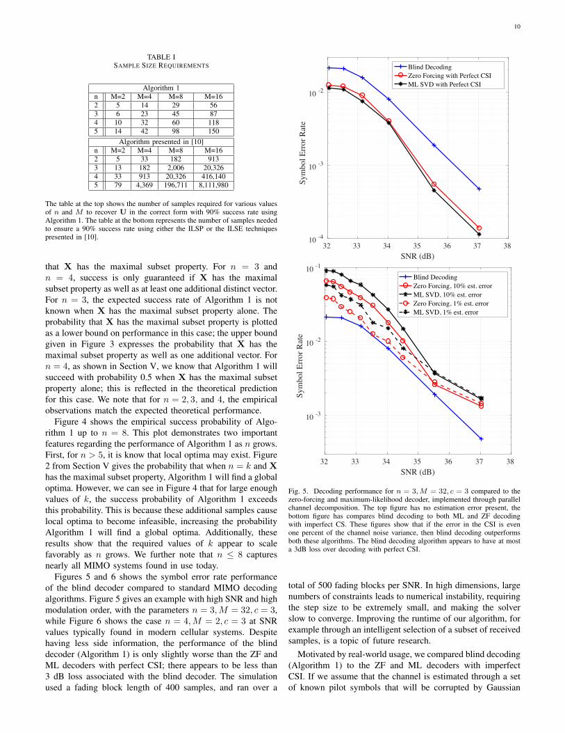
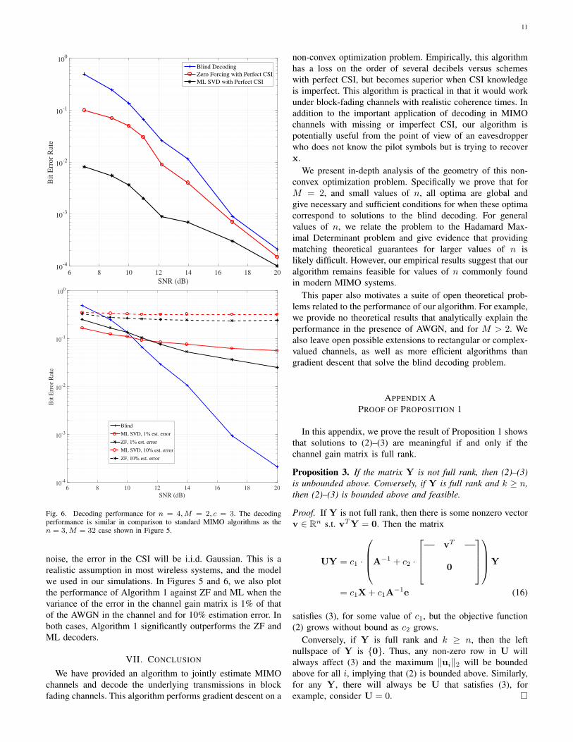
Figures 5 and 6 shows the symbol error rate performanceof the blind decoder compared to standard MIMO decodingalgorithms. Figure 5 gives an example with high SNR and highmodulation order, with the parameters n = 3,M = 32, c = 3,while Figure 6 shows the case n = 4,M = 2, c = 3 at SNRvalues typically found in modern cellular systems. Despitehaving less side information, the performance of the blinddecoder (Algorithm 1) is only slightly worse than the ZF andML decoders with perfect CSI; there appears to be less than3 dB loss associated with the blind decoder. The simulationused a fading block length of 400 samples, and ran over a

32 33 34 35 36 37 38SNR (dB)

10 -4

10 -3

10 -2

Sym

bol E

rror R

ate

Blind DecodingZero Forcing with Perfect CSIML SVD with Perfect CSI

32 33 34 35 36 37 38SNR (dB)

10 -3

10 -2

10 -1

Sym

bol E

rror

Rat

e

Blind DecodingZero Forcing, 10% est. errorML SVD, 10% est. errorZero Forcing, 1% est. errorML SVD, 1% est. error

Fig. 5. Decoding performance for n = 3,M = 32, c = 3 compared to thezero-forcing and maximum-likelihood decoder, implemented through parallelchannel decomposition. The top figure has no estimation error present, thebottom figure has compares blind decoding to both ML and ZF decodingwith imperfect CS. These figures show that if the error in the CSI is evenone percent of the channel noise variance, then blind decoding outperformsboth these algorithms. The blind decoding algorithm appears to have at mosta 3dB loss over decoding with perfect CSI.

total of 500 fading blocks per SNR. In high dimensions, largenumbers of constraints leads to numerical instability, requiringthe step size to be extremely small, and making the solverslow to converge. Improving the runtime of our algorithm, forexample through an intelligent selection of a subset of receivedsamples, is a topic of future research.

Motivated by real-world usage, we compared blind decoding(Algorithm 1) to the ZF and ML decoders with imperfectCSI. If we assume that the channel is estimated through a setof known pilot symbols that will be corrupted by Gaussian

11

6 8 10 12 14 16 18 20SNR (dB)

10-4

10-3

10-2

10-1

100Bi

t Erro

r Rat

e

Blind DecodingZero Forcing with Perfect CSIML SVD with Perfect CSI

6 8 10 12 14 16 18 20

SNR (dB)

10-4

10-3

10-2

10-1

100

Bit

Err

or

Rate

Blind

ML SVD, 1% est. error

ZF, 1% est. error

ML SVD, 10% est. error

ZF, 10% est. error

Fig. 6. Decoding performance for n = 4,M = 2, c = 3. The decodingperformance is similar in comparison to standard MIMO algorithms as then = 3,M = 32 case shown in Figure 5.

noise, the error in the CSI will be i.i.d. Gaussian. This is arealistic assumption in most wireless systems, and the modelwe used in our simulations. In Figures 5 and 6, we also plotthe performance of Algorithm 1 against ZF and ML when thevariance of the error in the channel gain matrix is 1% of thatof the AWGN in the channel and for 10% estimation error. Inboth cases, Algorithm 1 significantly outperforms the ZF andML decoders.

VII. CONCLUSION

We have provided an algorithm to jointly estimate MIMOchannels and decode the underlying transmissions in blockfading channels. This algorithm performs gradient descent on a

non-convex optimization problem. Empirically, this algorithmhas a loss on the order of several decibels versus schemeswith perfect CSI, but becomes superior when CSI knowledgeis imperfect. This algorithm is practical in that it would workunder block-fading channels with realistic coherence times. Inaddition to the important application of decoding in MIMOchannels with missing or imperfect CSI, our algorithm ispotentially useful from the point of view of an eavesdropperwho does not know the pilot symbols but is trying to recoverx.

We present in-depth analysis of the geometry of this non-convex optimization problem. Specifically we prove that forM = 2, and small values of n, all optima are global andgive necessary and sufficient conditions for when these optimacorrespond to solutions to the blind decoding. For generalvalues of n, we relate the problem to the Hadamard Max-imal Determinant problem and give evidence that providingmatching theoretical guarantees for larger values of n islikely difficult. However, our empirical results suggest that ouralgorithm remains feasible for values of n commonly foundin modern MIMO systems.

This paper also motivates a suite of open theoretical prob-lems related to the performance of our algorithm. For example,we provide no theoretical results that analytically explain theperformance in the presence of AWGN, and for M > 2. Wealso leave open possible extensions to rectangular or complex-valued channels, as well as more efficient algorithms thangradient descent that solve the blind decoding problem.

APPENDIX APROOF OF PROPOSITION 1

In this appendix, we prove the result of Proposition 1 showsthat solutions to (2)–(3) are meaningful if and only if thechannel gain matrix is full rank.

Proposition 3. If the matrix Y is not full rank, then (2)–(3)is unbounded above. Conversely, if Y is full rank and k ≥ n,then (2)–(3) is bounded above and feasible.

Proof. If Y is not full rank, then there is some nonzero vectorv ∈ Rn s.t. vTY = 0. Then the matrix

UY = c1 ·

A−1 + c2 ·

vT

0

Y

= c1X + c1A−1e (16)

satisfies (3), for some value of c1, but the objective function(2) grows without bound as c2 grows.

Conversely, if Y is full rank and k ≥ n, then the leftnullspace of Y is 0. Thus, any non-zero row in U willalways affect (3) and the maximum ‖ui‖2 will be boundedabove for all i, implying that (2) is bounded above. Similarly,for any Y, there will always be U that satisfies (3), forexample, consider U = 0.

12

APPENDIX BPROOF OF LEMMA 3

Lemma 3. If X has the maximal subset property, then, forall ATMs T, all matrices in the form U = TA−1, are globaloptima of (2)–(3).

Lemma 3 follows from the following claim.

Claim 2. Suppose that X has the maximal subset property.Then for all matrices M such that ‖Mx‖∞ ≤ 1 for all x ∈ X,we have |det M| ≤ 1.

Proof. Let x1, . . . ,xn be the set guaranteed by the maximalsubset property. Let V be the matrix whose columns arex1, . . . ,xn, so |det V| is maximal. If |det M| > 1, then|det MV| > |det V|. This would imply that MV cannotbe contained in [−1,+1]n×n.

Thus, if the matrix X has the maximal subset property, thenthe optimal solution to (2)–(3) have |det UA| = 1, and henceall U = TA−1 correspond to global optima. This completesthe proof of Lemma 3.

APPENDIX CPROOF OF THEOREM 1

Theorem 1. Algorithm 2 terminates at a vertex of the feasibleregion with probability 1.

We begin the proof of Theorem 1 with a lemma that isa simple consequence of the fact that the determinant is amultilinear function.

Lemma 4. All optima of (2)–(3) lie on the boundary of thefeasible region.

Proof. Consider a feasible, full-rank U which is not on theboundary of the feasible region, i.e. ‖Uyi‖∞ < 1 for alli ∈ [1, . . . , k]. Suppose |u(j)yi| = c for some i, j and some0 < c < 1. If we set:

u(j) = (1 + ε)u(j), (17)

for some 0 < ε ≤ c, and form U from the matrix U byreplacing row u(j) with u(j), then, because the determinant islinear in the rows of U, we have:

|det U| = (1 + ε)|det U| > |det U|, (18)

and U is still feasible.

In other words, if U is not on the problem boundary, themultilinearity of the determinant function implies that we canalways move towards the problem boundary (and away fromthe origin) in a way which increases the objective function.

We can also use the fact that the feasible region is formedby an n-dimensional polytope to further categorize the optimaof our optimization problem, as stated in the following lemma.Let P denote the polytope that describes the feasible regiongiven by (3), and let F denote a face of this polytope. Sinceeach row of the matrix U acts on the constraints in anindependent manner, we say that a row is “active” if thereare n linearly independent constraints active on this row. If allrows of U are active then U is a vertex of P; further, if there

are i active rows, then U lies on a face of dimension at mostn(n− i).

Lemma 5. Suppose that U is in the interior of a face F .Then there exists a v ∈ Rn, i ∈ [n], λ1 < λ2 ∈ R such thatthe interval I defined as

I = U + λeivᵀ|λ ∈ [λ1, λ2], (19)

satisfies I ⊆ F . Further, the points given by U + λjeivᵀ for

all j = 1, 2 lie on a face of lower dimension than F .

Proof. The polytope P is bounded by |〈u(j),y(i)〉| ≤ 1 fory(1), . . . ,y(k) and all rows u(j) of U. If U is not at a vertex,then there exists a row u(j) that is not active. For this non-active row u(j), say that Ω = y(i) | |〈u(j),y(i)〉| = 1. Wemust have dim(Ω) < n. Thus, there exists a v ∈ Ω⊥ and ay(i) /∈ cols(Y) such that 〈v,y(i)〉 6= 0. This is true since if,for all y(i) ∈ Y, 〈v,y(i)〉 = 0, then Y is not full rank. Wenow require the following claim:

Claim 3. For small enough λ, U + λejvᵀ ∈ F .

Proof. The quantity λejvᵀ only affects constraints acting on

row j of U, and for all y(i) ∈ Ω, (U+λejvᵀ) ·y(i) = Uy(i).

Thus, no active constraints have been affected which impliesthat we have not left the face F .

It remains to show that for appropriate values of λ1 and λ2,the points given by U + λjeiv

ᵀ, for all j = 1, 2, lie on alower dimensional face than F . Since there exists a y(i) suchthat 〈v,y(i)〉 6= 0, there must be exactly two values λ1, λ2such that 〈uj +λiejv

ᵀ,y(j)〉 = ±1. Thus, for these boundingvalues of λ, an additional constraint will be active, implyingthat U + λjeiv

ᵀ will be on a lower dimensional face thanF .

Having established Lemma 5, we now show the followingcorollary which allow us to further characterize the optima of(2)–(3).

Corollary 1. Non-strict optima (which by Lemma 4 mustlie on a face F) are restricted to an interval I as given in(19). Further, the end points of this interval lie in a lowerdimensional face.

Proof. Suppose U is a non-strict optima in the interior of someface. By Lemma 5 and the multilinearity of the determinant,there must exist an interval I over which the objective functionis constant valued.

We also remark, informally, that Lemma 5 also implies thatall strict optima will in fact be vertices of the feasible region.By Lemma 5 and Corollary 1, for any U that lies on theinterior of a face, U is not a strict optimum. Indeed, theremust either be a direction eiv

ᵀ along which U may moveeither to increase the value of the objective function or keepthe objective function constant. This result is not needed tocomplete Theorem 1, but provides insight into the geometryof the problem.

Having characterized the set of optima in (2)–(3), we nowturn our attention to characterizing the behavior of Algorithms

13

1 and 2. To do so, we will consider the gradient of the objectivefunction, which is given in [20], as

∇ log |det U| =(U−1

)ᵀ. (20)

We note that an alternative proof of Lemma 4 follows fromthe fact that the gradient is non-zero as long as U is finite.

In order to understand how gradient descent will behaveon the boundary of the feasible region, we must considerdirectional derivatives for directions that lie on the problemboundary. Let ∆ ∈ Rn×n be a direction such that, for feasibleU, U + ∆ is also feasible. Gradient descent will terminate if,for all ∆, ⟨(

U−1)ᵀ,∆⟩F≤ 0, (21)

where 〈·, ·〉F is the Frobenius inner product. Thus, (21) is equalto vec

((U−1

)ᵀ)ᵀvec(∆) or tr(

(U−1

)ᵀ∆).

We now show that (21) can only hold if each row has eithern−1 or n active, linearly independent constraints. This lemma,as well as Corollary 1, motivate Algorithm 2 as it impliesthat there may be corner cases where Algorithm 1 will fail,but these corner cases can easily be handled by forcing thealgorithm to terminate at the nearest vertex.

Lemma 6. If any row of U has fewer then n − 1 activeconstraints, then there exists a non-zero matrix ∆ such thatU + ∆ satisfies (3) and log |det U + ∆| > log |det U|

Proof. Consider the ith row of U, denoted u(i), and let δ(i)

be the corresponding elements of ∆. The corresponding rowof the gradient matrix is given by:

(∇U)(i)

=1

det Uc(i), (22)

where c(i) is the ith row of the cofactor matrix of U. SinceU must be full rank, c(i) must be non-zero for all i. Thus, forany i, the only way in which we could have

1

det U

⟨c(i), δ(i)

⟩F

= 0 (23)

is if the only feasible values of δ(i) (i.e. those that do not moveU outside the feasible region) are orthogonal to c(i).

If fewer than n − 1 linearly independent constraints areactive on the ith row, then there always is a subspace of atleast dimension two from which we can select δ(i). Precisely,suppose that the constraints given by y1, . . . , yn−2 are active.The subspace spanned by these vectors must always have anull space of at least dimension two; if δ(i) is contained inthis nullspace then U + ∆ will be feasible. As long as thisnullspace has dimension at least two, for all i, there exists aδ(i) such that U + ∆ satisfies (3) and that has 〈c(i), δ(i)〉 6= 0.Thus, gradient descent will always proceed as long as fewerthan n− 1 constraints are active on each row.

In other words, by Lemma 6, if gradient descent terminatesand we are not at a vertex, there must be at least one rowwith exactly n − 1 active, linearly independent constraints.In this case, we may move along the interval I guaranteedby Corollary 1 until we reach a lower dimensional face.This lower dimensional face will either be a vertex, in which

case we have reached a strict optima and the algorithm willterminate, or there will exist a positive gradient and we canresult gradient descent. This completes Theorem 1.

APPENDIX DPROOF OF THEOREM 3

Theorem 3. When n = 3, Algorithm 2 is correct withprobability 1 if and only if k ≥ 4 and there exists a 3×4 matrixV, such that cols(V) ⊆ cols(X), span(v1, . . . ,v4) = R3, andall vectors in V are pair-wise linearly independent.

We know that if X has the maximal subset property, thenAlgorithm 2 will always terminate at a global maximum of(2)–(3) and that the set of global optima contains all solutionsin the form TX for all T ∈ T . However, for n = 3,the maximal subset property alone does not ensure that allglobal optima will be solutions to the blind decoding problem.Spurious optima must have the form QX ∈ [−1,+1]n×k,where det Q = ±1 and Q /∈ T . Algorithm 2 will only becorrect with probability 1 if there are no spurious optima.

We now show that, for n = 3, if X has four distinctcolumns (distinct meaning pair-wise linearly independent),QX ∈ [−1,+1]n×k and det Q = ±1 implies that Q ∈ T .This further implies that all global optima are solutions to theblind decoding problem. Consider the following choice of X:

X =

1 1 −1 −11 −1 1 −11 1 1 1

. (24)

The following lemma shows that this choice of X furtherrestricts Q to be orthogonal.

Lemma 7. Suppose Q has det Q = ±1, and, for X given by(24), if QX ∈ [−1,+1]3×3, then Q ∈ O(3).

Proof. We know that, by Theorem 1, Algorithm 2 must ter-minate at a vertex. Thus, we must have QX ∈ −1,+1n×k,which further implies that, for all i, ‖Qxi‖2 = ‖xi‖2. Wenow consider the set of linear operators with determinant ±1whose action preserves the norms of each vector xi.

Define the operator Q = ΣVᵀ, where Σ denotes thediagonal matrix containing the singular values of Q and Vdenotes the right singular vectors of Q. Since Q = UQ, forsome U ∈ O(3), there must exist a Q such that Qxi = ±xi

for all i; otherwise, ‖Qxi‖2 6= ‖xi‖2 for some i.We can consider the action of any Q on the surface of

a sphere of radius√

3. This sphere, S, contains the vectorsthat comprise the columns of X. Under the action of anylinear operator with determinant ±1, S will be mapped to anellipsoid, E , such that vol(E) = vol(S). Further, we know thatE , given by Q, must contain the points xi for all i. Lemma 7is now completed by Claim 4, which shows that this is onlypossible if E = S, implying that Q ∈ O(3).

Claim 4. The only ellipsoid that is centered on the origin, hasvolume 4π

√3, and contains the points given by cols(X) is a

sphere.

14

Proof. Consider an arbitrary ellipsoid, E , centered about theorigin. For some A 0, this can be described by the followingequation

vᵀAv = 1

[x y z

] a d2

f2

d2 b e

2f2

e2 c

xyz

= 1. (25)

We require the ellipsoid to contain the points (±1,±1, 1). Bysubstituting these points into (25), it is seen that we must haved = e = f = 0 and a+ b+ c = 1. Thus, A must be diagonal.

The eigenvalues of A are the inverse squares of the lengthof the semi-axes of the ellipsoid. This implies that the volumeof the ellipsoid is given by vol(E) = 4

3π/√abc. The only

solution that gives vol(E) = 4π√

3 with a + b + c = 1 isa = b = c = 1

3 , implying that the required ellipsoid in fact asphere.

Having established that (24) implies that Q ∈ O(3), wecan further show that the only feasible elements of O(3) arein fact the ATMs.

Proposition 2. Suppose Q has Q ∈ O(3), and QX ∈[−1,+1]3×4, then Q ∈ T .

Proof. Notice that the vectors cols(X) form a face of theunit cube. Since QX ∈ [−1,+1]3×4 and Q ∈ O(3), thencols(QX) must also form the face of a unit cube. This isbecause Q is orthogonal and must preserve norms and planes.This fact restricts Q to the symmetries of the cube. There are48 symmetries of the cube, which correspond to the set of 48ATMs.

Finally notice that for all D = diag(±1, . . . ,±1), QX ∈[−1,+1]n×k implies that QXD ∈ [−1,+1]n×k. Similarly, forall permutation matrices P. For n = 3, all possible ±1-valuedmatrices that contain four distinct columns can be expressedas XPD. This implies that if QX ∈ [−1,+1]3×4, for anypossible X with four distinct columns, then Q ∈ T . Hence,any choice of X with four distinct columns is sufficient toensure that there are no spurious optima.

We now turn our attention to showing the converse: thatrequiring X to have four distinct columns (that is, pairwiselinearly independent) is in fact necessary for Algorithm 2to be correct with probability 1. First, if n = k = 3, thenfor any choice of X such that X has the maximal subsetproperty spurious optima will exist. For n = 3, there is asmall collection of three vectors, up to the ATMs, that havethe maximal subset property, and so one may check that this isalways true. Therefore, when n = k = 3, there will always bea matrix Q with unit determinant such that QX ∈ [−1,+1]3×3

and Q /∈ T .If X does not have four distinct columns then this will

always be the case. Consider the case that k > 3 and X hasthe maximal subset property but no four columns of X aredistinct. Let the matrix V be formed from any subset of threecolumns of X such that V has the maximal subset property.Then we must have that for all i, there exists a j such thatxi = ±vj . For any Qvj ∈ [−1,+1]n, we also must have

−Qvj = Qxi ∈ [−1,+1]n. Thus, whenever X does notcontain any columns that are distinct from the columns ofV, then X will also have the same set of optima as V. Thiscompletes Theorem 3.

APPENDIX EPROOF OF THEOREM 4

In this appendix we prove Theorem 4, which gives necessaryand sufficient conditions so that Algorithms 1 and 2 returncorrect solutions to the blind decoding problem when n = 4.Notice that because a Hadamard matrix exists at n = 4, weknow by Lemma 2 the only optima are strict and are verticesof the feasible region. Thus Algorithm 2 is not needed in thiscase. Before considering the specific case of n = 4, we provethe following more general statement for values of n such thata Hadamard matrix exists. This result will be used in the proofof Theorem 4. When a Hadamard matrix exists, we can furthercharacterize the solutions to (2)–(3) in the noiseless case asfollows.

Lemma 8. If n is such that Hadamard matrix exists, and Xhas the maximal subset property, then the only global optimato (2)–(3) on input Y = AX are of the form U = QA−1,where Q ∈ O(n).

The following claim is helpful in proving this lemma:

Claim 5. For X ∈ Rn×n is an orthogonal matrix and someM ∈ Rn×n with |det M| = 1, if ‖Mxi‖2 ≤ ‖xi‖2 for all i,then M must be orthogonal.

Proof. Let x1, . . . ,xn be the orthonormal basis obtained bythe columns of X.

tr(MTM

)=∥∥MTM

∥∥2F

=

n∑i=1

|λi|2 (26)∣∣∣∣∣n∑

i=1

xTi MTMxi

∣∣∣∣∣ ≤n∑

i=1

|xTi MTMxi| (27)

=

n∑i=1

|Mxi|2 (28)

≤n∑

i=1

|xi|2 (29)

= n (30)

However, because |det M| = 1, this implies:

det MTM =

n∏i=1

λ2i = 1 =

n∑i=1

|λi|2, (31)

and by the inequality of arithmetic and geometric means, thisimplies λ2i = 1 for all i. Since M is real valued, this impliesM is orthogonal.

By Lemma 2, we know that Q must have determinantone. Let V be the matrix guaranteed by the maximal subsetproperty. V must be Hadamard. The matrix UAV, willalso have the maximum value of the determinant over all[−1,+1]n×n matrices, and thus must also be Hadamard. Sinceall points in V and UAV have `2-norm 2n/2, by Claim 5,

15

UA must be orthogonal. This completes the proof of Lemma8.

At this point, one might be tempted to conjecture that, infact, the maximal subset property is on its own sufficient; thatis that the orthogonal matrix Q in Lemma 8 can be replacedby an ATM T. However, this is not the case as we will showin the proof of Theorem 4, given below.

Theorem 4. When n = 4, Algorithm 1 is correct withprobability 1 if and only if k ≥ 5 and cols(X) contains atleast four linearly independent vectors from H(i)

4 and a fifthvector from H(j)

4 for any i 6= j.Algorithm 1 will be correct with probability 0.5 if cols(X)

has only four linearly independent vectors belonging to thesame equivalence class.

We prove Theorem 4 in two parts. First, in Lemma 9,we show that when n = k and X has the maximal subsetproperty, Algorithm 1 will return the correct solution to theblind decoding problem with probability 0.5, and that withthe addition of an extra vector from a separate equivalenceclass, all global optima correspond to solutions to the blinddecoding problem. In Lemma 9 we in fact prove a slightlymore general statement and give the probability of that allglobal optima correspond to solutions of the blind decodingproblem given the input to Algorithm 1 is chosen uniformlyat random. Second, in Lemma 10, we show that for all valuesof k, all optima are indeed global despite the fact that thereare suboptimal vertices.

Lemma 9. For n = 4, for a collection of k samples chosenuniformly at random, the probability that all global optimawill correspond to solutions of the blind decoding problem isgiven by

Pr(Success) = r(4, k) · r(3, k)4 · (1− 2n−k). (32)

Proof. One can verify that for n = 4, for a matrix to have themaximal subset property (and hence be a Hadamard matrix),then not only must the matrix be full rank, but all matricesobtained by choosing a subset of three rows must also befull rank. The probability that a random set of k vectors ofdimension 4 is a Hadamard matrix given by:

Pr(Success) = r(4, k) · r(3, k)4. (33)

It can be seen that there is an orthogonal matrix, S, that is notan ATM, such that for all G ∈ H(1)

4 , and H ∈ H(2)4 , G = SH.

To find an example of such a matrix, for any choice of G andH, compute S = G−1H. This implies that, exactly half of theglobal optima are solutions to (2)–(3). This is consistent withthe observation that if X has a maximal subset, then Algorithm1 succeeds 50% of the time for n = 4, k = 4.

Notice that for this same G,H, and S given above, SG /∈−1,+14 and similarly S−1H /∈ −1,+14, for all G andH. Notice further that all vectors in −1,+14 appear in eitherH(1)

4 or H(2)4 , and that the product of S times any vector in

H(1)4 is not in −1,+14. Similarly, any S−1 times any H(2)

4

is not in −1,+14.Now consider a collection of k > n vectors that contains

4 independent elements of H(i)4 , for some i. If all vectors

in this collection belong to the same equivalence class, thenmatrices containing a factor of S will be the optima of (2)–(3).Otherwise, all such matrices will lie outside of the feasibleregion and all global optima will correspond to solutions.For this reason, adding constraints removes vertices fromthe feasible region, thus increasing the success probability ofAlgorithm 2.

Given the above argument, we have a probability of 1−2n−k

that the only global optima will be solutions, conditioned onthe fact that the matrix has the maximal subset property. Sinceequation (33) gives the probability of the maximum subsetholding, we can express the probability that, given k randomsamples, all global optima are solutions to (2)–(3) as:

Pr(Success) = r(4, k) · r(3, k)4 · (1− 2n−k). (34)

In order to arrive at our desired result for n = 4, we stillneed to show that no vertices that correspond to matrices withdeterminant of ±8 are local optima of (2)–(3). This is provenbelow and completes Theorem 4.

Lemma 10. For n = 4, all optima of (2)–(3) are global.

Proof. Optima of (2)–(3) can only lie on vertices of theproblem boundary — that is optima can only correspond tonon-singular ±1-valued matrices by Lemma 2. We need toshow that no matrices with determinant ±8 are local optima.We begin with two facts which have been verified throughcomputer simulation.

Create a graph with a node for each matrix in −1, 14×4and edges between each pair of nodes that have Hammingdistance of one. Remove from this graph all nodes whichcorrespond two determinant zero, leaving only nodes withdeterminant ±8 and ±16. Since the determinant is a linearfunction of the columns of a matrix, then the value of det Achanges linearly along each edge of this graph. Studying thegeometry of this graph will give us insight into paths thatAlgorithm 2 may travel in arriving to an optima.

The first observation is that the graph is partitioned intotwo components. This can be verified, for example, eitherby inspecting the least eigenvalues of the Laplacian of theadjacency matrix of the graph or performing a breadth-firstsearch. We find that one component of this graph correspondsto ±1-valued matrix that have positive determinants, and theother to all all matrices with negative determinants. This meansthat one can traverse either component of these graphs withoutthe objective function changing sign. This further implies that,over each edge of the graph, the objective function is eitherconstant (and equal to log 8 along each edge), or changeslogrithmically from log 8 to log 16.

It can further be verified that the maximum Hamming dis-tance between any matrix of determinant ±8 and determinant±16 is 2. Those that have Hamming distance 1 are clearlynot local optima. Thus we turn our attention to the remainingdeterminate ±8 matrices that have Hamming distance 2. Eachof matrices is connected to at least two determinant ±8matrices that are distance 1 away from a ±16 matrix. This

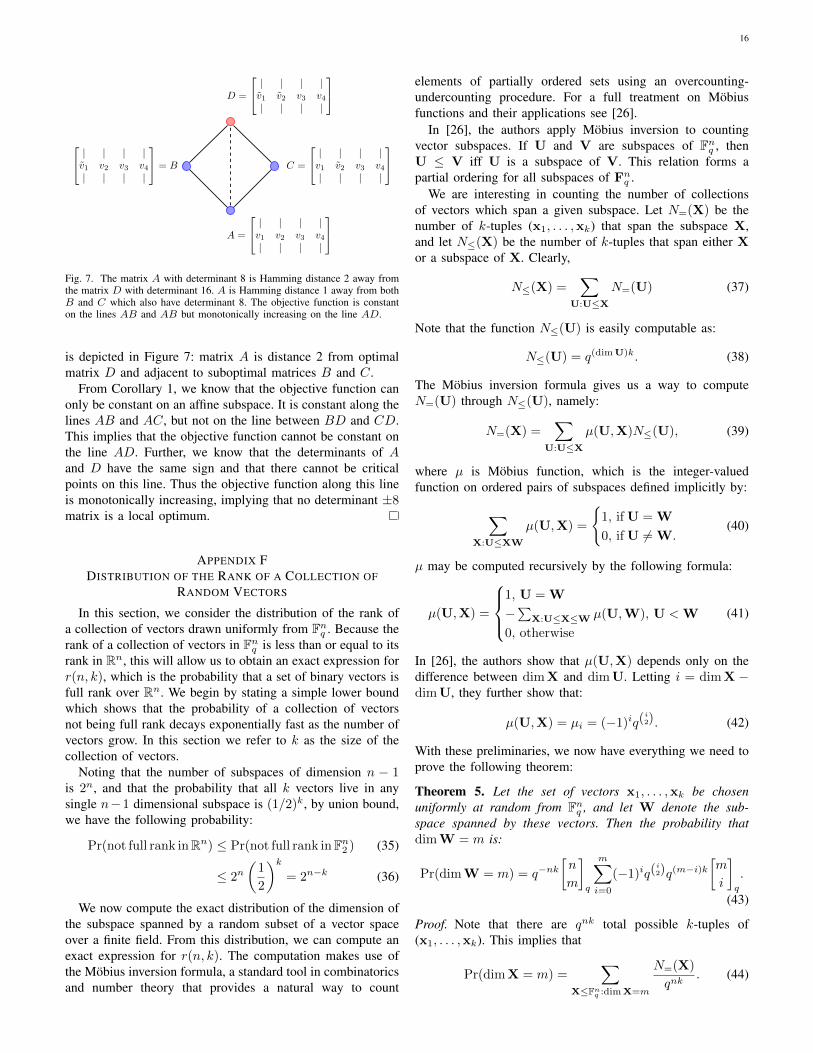
16

A =

| | | |v1 v2 v3 v4| | | |

| | | |v1 v2 v3 v4| | | |

= B C =

| | | |v1 v2 v3 v4| | | |

D =

| | | |v1 v2 v3 v4| | | |

Fig. 7. The matrix A with determinant 8 is Hamming distance 2 away fromthe matrix D with determinant 16. A is Hamming distance 1 away from bothB and C which also have determinant 8. The objective function is constanton the lines AB and AB but monotonically increasing on the line AD.

is depicted in Figure 7: matrix A is distance 2 from optimalmatrix D and adjacent to suboptimal matrices B and C.

From Corollary 1, we know that the objective function canonly be constant on an affine subspace. It is constant along thelines AB and AC, but not on the line between BD and CD.This implies that the objective function cannot be constant onthe line AD. Further, we know that the determinants of Aand D have the same sign and that there cannot be criticalpoints on this line. Thus the objective function along this lineis monotonically increasing, implying that no determinant ±8matrix is a local optimum.

APPENDIX FDISTRIBUTION OF THE RANK OF A COLLECTION OF

RANDOM VECTORS

In this section, we consider the distribution of the rank ofa collection of vectors drawn uniformly from Fn

q . Because therank of a collection of vectors in Fn

q is less than or equal to itsrank in Rn, this will allow us to obtain an exact expression forr(n, k), which is the probability that a set of binary vectors isfull rank over Rn. We begin by stating a simple lower boundwhich shows that the probability of a collection of vectorsnot being full rank decays exponentially fast as the number ofvectors grow. In this section we refer to k as the size of thecollection of vectors.

Noting that the number of subspaces of dimension n − 1is 2n, and that the probability that all k vectors live in anysingle n−1 dimensional subspace is (1/2)k, by union bound,we have the following probability:

Pr(not full rank inRn) ≤ Pr(not full rank inFn2 ) (35)

≤ 2n(

1

2

)k

= 2n−k (36)

We now compute the exact distribution of the dimension ofthe subspace spanned by a random subset of a vector spaceover a finite field. From this distribution, we can compute anexact expression for r(n, k). The computation makes use ofthe Mobius inversion formula, a standard tool in combinatoricsand number theory that provides a natural way to count

elements of partially ordered sets using an overcounting-undercounting procedure. For a full treatment on Mobiusfunctions and their applications see [26].

In [26], the authors apply Mobius inversion to countingvector subspaces. If U and V are subspaces of Fn

q , thenU ≤ V iff U is a subspace of V. This relation forms apartial ordering for all subspaces of Fn

q .We are interesting in counting the number of collections

of vectors which span a given subspace. Let N=(X) be thenumber of k-tuples (x1, . . . ,xk) that span the subspace X,and let N≤(X) be the number of k-tuples that span either Xor a subspace of X. Clearly,

N≤(X) =∑

U:U≤X

N=(U) (37)

Note that the function N≤(U) is easily computable as:

N≤(U) = q(dimU)k. (38)

The Mobius inversion formula gives us a way to computeN=(U) through N≤(U), namely:

N=(X) =∑

U:U≤X

µ(U,X)N≤(U), (39)

where µ is Mobius function, which is the integer-valuedfunction on ordered pairs of subspaces defined implicitly by:

∑X:U≤XW

µ(U,X) =

1, if U = W

0, if U 6= W.(40)

µ may be computed recursively by the following formula:

µ(U,X) =

1, U = W

−∑

X:U≤X≤W µ(U,W), U < W

0, otherwise

(41)

In [26], the authors show that µ(U,X) depends only on thedifference between dim X and dim U. Letting i = dim X −dim U, they further show that:

µ(U,X) = µi = (−1)iq(i2). (42)

With these preliminaries, we now have everything we need toprove the following theorem:

Theorem 5. Let the set of vectors x1, . . . ,xk be chosenuniformly at random from Fn

q , and let W denote the sub-space spanned by these vectors. Then the probability thatdim W = m is:

Pr(dim W = m) = q−nk[n

m

]q

m∑i=0

(−1)iq(i2)q(m−i)k

[m

i

]q

.

(43)

Proof. Note that there are qnk total possible k-tuples of(x1, . . . ,xk). This implies that

Pr(dim X = m) =∑

X≤Fnq :dimX=m

N=(X)

qnk. (44)

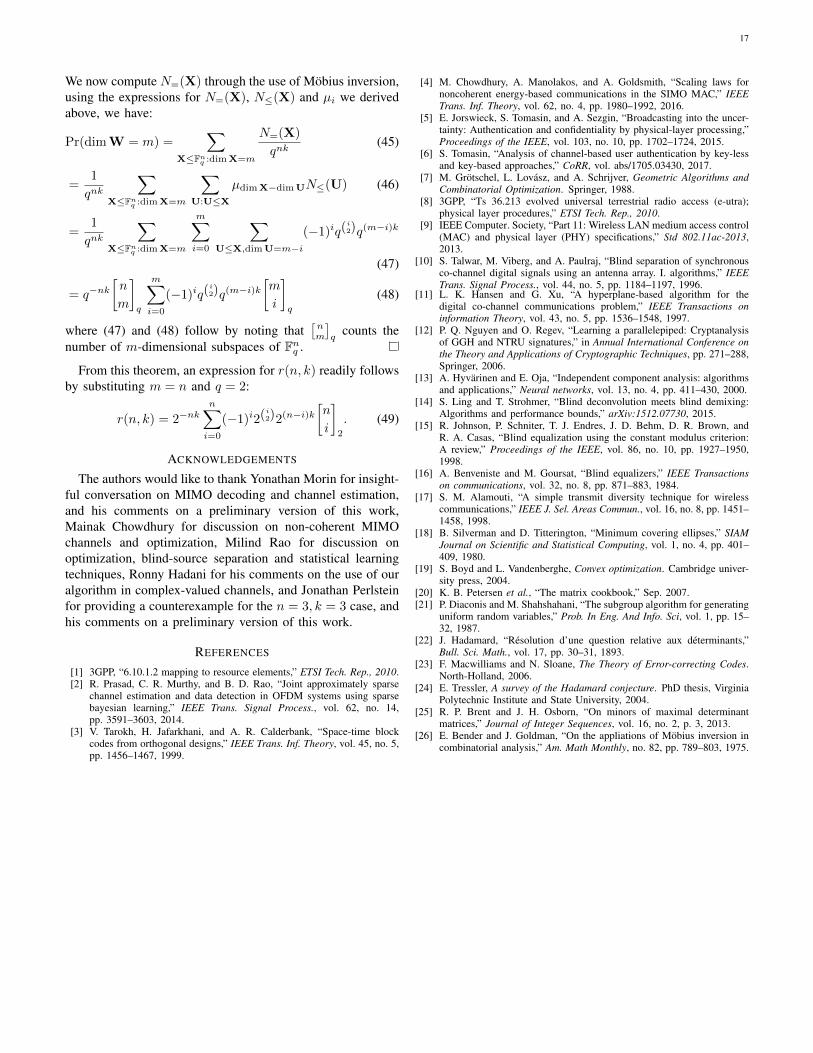
17

We now compute N=(X) through the use of Mobius inversion,using the expressions for N=(X), N≤(X) and µi we derivedabove, we have:

Pr(dim W = m) =∑

X≤Fnq :dimX=m

N=(X)

qnk(45)

=1

qnk

∑X≤Fn

q :dimX=m

∑U:U≤X

µdimX−dimUN≤(U) (46)

=1

qnk

∑X≤Fn

q :dimX=m

m∑i=0

∑U≤X,dimU=m−i

(−1)iq(i2)q(m−i)k

(47)

= q−nk[n

m

]q

m∑i=0

(−1)iq(i2)q(m−i)k

[m

i

]q

(48)

where (47) and (48) follow by noting that[nm

]q

counts thenumber of m-dimensional subspaces of Fn

q .

From this theorem, an expression for r(n, k) readily followsby substituting m = n and q = 2:

r(n, k) = 2−nkn∑

i=0

(−1)i2(i2)2(n−i)k

[n

i

]2

. (49)

ACKNOWLEDGEMENTS

The authors would like to thank Yonathan Morin for insight-ful conversation on MIMO decoding and channel estimation,and his comments on a preliminary version of this work,Mainak Chowdhury for discussion on non-coherent MIMOchannels and optimization, Milind Rao for discussion onoptimization, blind-source separation and statistical learningtechniques, Ronny Hadani for his comments on the use of ouralgorithm in complex-valued channels, and Jonathan Perlsteinfor providing a counterexample for the n = 3, k = 3 case, andhis comments on a preliminary version of this work.

REFERENCES

[1] 3GPP, “6.10.1.2 mapping to resource elements,” ETSI Tech. Rep., 2010.[2] R. Prasad, C. R. Murthy, and B. D. Rao, “Joint approximately sparse

channel estimation and data detection in OFDM systems using sparsebayesian learning,” IEEE Trans. Signal Process., vol. 62, no. 14,pp. 3591–3603, 2014.

[3] V. Tarokh, H. Jafarkhani, and A. R. Calderbank, “Space-time blockcodes from orthogonal designs,” IEEE Trans. Inf. Theory, vol. 45, no. 5,pp. 1456–1467, 1999.

[4] M. Chowdhury, A. Manolakos, and A. Goldsmith, “Scaling laws fornoncoherent energy-based communications in the SIMO MAC,” IEEETrans. Inf. Theory, vol. 62, no. 4, pp. 1980–1992, 2016.

[5] E. Jorswieck, S. Tomasin, and A. Sezgin, “Broadcasting into the uncer-tainty: Authentication and confidentiality by physical-layer processing,”Proceedings of the IEEE, vol. 103, no. 10, pp. 1702–1724, 2015.

[6] S. Tomasin, “Analysis of channel-based user authentication by key-lessand key-based approaches,” CoRR, vol. abs/1705.03430, 2017.

[7] M. Grotschel, L. Lovasz, and A. Schrijver, Geometric Algorithms andCombinatorial Optimization. Springer, 1988.

[8] 3GPP, “Ts 36.213 evolved universal terrestrial radio access (e-utra);physical layer procedures,” ETSI Tech. Rep., 2010.

[9] IEEE Computer. Society, “Part 11: Wireless LAN medium access control(MAC) and physical layer (PHY) specifications,” Std 802.11ac-2013,2013.

[10] S. Talwar, M. Viberg, and A. Paulraj, “Blind separation of synchronousco-channel digital signals using an antenna array. I. algorithms,” IEEETrans. Signal Process., vol. 44, no. 5, pp. 1184–1197, 1996.

[11] L. K. Hansen and G. Xu, “A hyperplane-based algorithm for thedigital co-channel communications problem,” IEEE Transactions oninformation Theory, vol. 43, no. 5, pp. 1536–1548, 1997.

[12] P. Q. Nguyen and O. Regev, “Learning a parallelepiped: Cryptanalysisof GGH and NTRU signatures,” in Annual International Conference onthe Theory and Applications of Cryptographic Techniques, pp. 271–288,Springer, 2006.

[13] A. Hyvarinen and E. Oja, “Independent component analysis: algorithmsand applications,” Neural networks, vol. 13, no. 4, pp. 411–430, 2000.

[14] S. Ling and T. Strohmer, “Blind deconvolution meets blind demixing:Algorithms and performance bounds,” arXiv:1512.07730, 2015.

[15] R. Johnson, P. Schniter, T. J. Endres, J. D. Behm, D. R. Brown, andR. A. Casas, “Blind equalization using the constant modulus criterion:A review,” Proceedings of the IEEE, vol. 86, no. 10, pp. 1927–1950,1998.

[16] A. Benveniste and M. Goursat, “Blind equalizers,” IEEE Transactionson communications, vol. 32, no. 8, pp. 871–883, 1984.

[17] S. M. Alamouti, “A simple transmit diversity technique for wirelesscommunications,” IEEE J. Sel. Areas Commun., vol. 16, no. 8, pp. 1451–1458, 1998.

[18] B. Silverman and D. Titterington, “Minimum covering ellipses,” SIAMJournal on Scientific and Statistical Computing, vol. 1, no. 4, pp. 401–409, 1980.

[19] S. Boyd and L. Vandenberghe, Convex optimization. Cambridge univer-sity press, 2004.

[20] K. B. Petersen et al., “The matrix cookbook,” Sep. 2007.[21] P. Diaconis and M. Shahshahani, “The subgroup algorithm for generating

uniform random variables,” Prob. In Eng. And Info. Sci, vol. 1, pp. 15–32, 1987.

[22] J. Hadamard, “Resolution d’une question relative aux determinants,”Bull. Sci. Math., vol. 17, pp. 30–31, 1893.

[23] F. Macwilliams and N. Sloane, The Theory of Error-correcting Codes.North-Holland, 2006.

[24] E. Tressler, A survey of the Hadamard conjecture. PhD thesis, VirginiaPolytechnic Institute and State University, 2004.

[25] R. P. Brent and J. H. Osborn, “On minors of maximal determinantmatrices,” Journal of Integer Sequences, vol. 16, no. 2, p. 3, 2013.

[26] E. Bender and J. Goldman, “On the appliations of Mobius inversion incombinatorial analysis,” Am. Math Monthly, no. 82, pp. 789–803, 1975.