Embed Size (px)
Citation preview
University of North DakotaUND Scholarly Commons
Theses and Dissertations Theses, Dissertations, and Senior Projects
January 2014
Antenna Selection And MIMO CapacityEstimation For Vehicular Communication SystemsNischal Adhikari
Follow this and additional works at: https://commons.und.edu/theses
This Thesis is brought to you for free and open access by the Theses, Dissertations, and Senior Projects at UND Scholarly Commons. It has beenaccepted for inclusion in Theses and Dissertations by an authorized administrator of UND Scholarly Commons. For more information, please [email protected].
Recommended CitationAdhikari, Nischal, "Antenna Selection And MIMO Capacity Estimation For Vehicular Communication Systems" (2014). Theses andDissertations. 1497.https://commons.und.edu/theses/1497
ANTENNA SELECTION AND MIMO CAPACITY ESTIMATION FOR VEHICULAR COMMUNICATION SYSTEMS
By
Nischal Adhikari
A Thesis Submitted to the Graduate Faculty
of the
University of North Dakota
In partial fulfillment of the requirements
for the degree of
Masters of Science
Grand Forks, North Dakota May 2014

ii
Copyright 2014 Nischal Adhikari

iv
Title ANTENNA SELECTION AND MIMO CAPACITY ESTIMATION FOR
VEHICULAR COMMUNICATION SYSTEMS Department Electrical Engineering Degree Masters of Science In presenting this thesis in partial fulfillment of the requirements for a graduate degree from the University of North Dakota, I agree that the library of this University shall make it freely available for inspection. I further agree that permission for extensive copying for scholarly purposes may be granted by the professor who supervised my thesis work or, in her absence, by the Chairperson of the department or the dean of the Graduate School. It is understood that any copying or publication or other use of this thesis or part thereof for financial gain shall not be allowed without my written permission. It is also understood that due recognition shall be given to me and to the University of North Dakota in any scholarly use which may be made of any material in my thesis. Nischal Adhikari DATE: May 2014
v
TABLE OF CONTENTS
LIST OF FIGURES ...................................................................................................................... viii
LIST OF TABLES ........................................................................................................................... x
LIST OF SYMBOLS……………………………………………………………………………...xii
ABBREVIATIONS ……………………………………………………………………………...xiii
ACKNOWLEDGEMENTS ........................................................................................................... xv
ABSTRACT………… .................................................................................................................. xvi
CHAPTER
1 Introduction ......................................................................................................................... 1
1.1 Motivation .............................................................................................................. 1
1.2 Thesis Outline ........................................................................................................ 3
2 Literature Review................................................................................................................ 5
2.1 Introduction to Vehicular Communications ........................................................... 5
2.2 Development of V2V Communication Standards ................................................. 7
2.3 V2V Communications’ Prospective Applications ............................................... 13
2.4 Vehicular Propagation Path ................................................................................. 17
2.5 MIMO in Vehicular Communication ................................................................... 20
2.6 MIMO Capacity ................................................................................................... 22
vi
2.7 Simulation and Measurement .............................................................................. 25
2.8 Summary .............................................................................................................. 27
3 Multiple Antenna Systems for Vehicle to Vehicle Communications ............................... 28
3.1 Methodology ........................................................................................................ 29
3.1.1 System Set Up……………………………………………………………..29
3.1.2 Environment Modeling…………………………………………………….30
3.1.3 Implementing MIMO System……………………………………………...33
3.2 Results and Discussion……………………………………………………... .. …34
3.3 Summary .............................................................................................................. 42
4 Effects of Blockage on the MIMO Capacity for DSRC Channels .................................... 44
4.1 Introduction .......................................................................................................... 44
4.2 Methodology ........................................................................................................ 45
4.2.1 System Set Up……………………………………………………………..46
4.2.2 Environment Modeling…………………………………………………….46
4.2.3 Implementing MIMO Systems…………………………………………….48
4.3 Results .................................................................................................................. 50
4.3.1 Effects of the Antenna Location, Power, and Phase on the Capacity……..50
4.3.2 Graphical representations of Capacity vs. SNR…………………………...56
4.3.3 Effect of Phase Factor……………………………………………………...62
4.3.4 K Factor……………………………………………………………………63
4.4 Summary .............................................................................................................. 66
5 Measurement Setup and Results ....................................................................................... 68
5.1 Introduction .......................................................................................................... 68
5.2 System Configuration .......................................................................................... 70
5.2.1 Hardware…………………………………………………………………..70
vii
5.2.2 Software……………………………………………………………………73
5.3 Methodology ........................................................................................................ 75
5.3.1 System Set Up……………………………………………………………..76
5.3.2 Operation Procedure……………………………………………………….79
5.3.3 Data Processing……………………………………………………………82
5.4 Results and Discussions ....................................................................................... 82
5.5 Summary .............................................................................................................. 92
6 Future Work and Conclusion ............................................................................................ 93
6.1 Dynamic Measurement ........................................................................................ 93
6.2 Channel Sounding Techniques ............................................................................ 94
6.3 Cognitive Radio ................................................................................................... 94
6.4 Conclusion ........................................................................................................... 94
APPENDICES….. ......................................................................................................................... 96
REFERENCES…………………………………………………………………………………..102
viii
LIST OF FIGURES
Figures Page 1 Inter vehicular communication [10]. 6
2 Wave architecture [13]. 7
3 CALM architecture [13]. 8
4 C2C-CC architecture [13]. 8
5 Milestone is vehicular communication [10]. 11
6 WAVE, IEEE 1609, 802.11p and the OSI reference model [17]. 12 7 DSRC channel frequency assignments [24]. 13
8 V2V communication prospective applications [14]. 15 9 A MIMO system model with N transmitter and M receiver and
channel matrix H [49]. 23
10 Layout of antenna positions and their assigned numbers in transmitting and receiving vehicles.
30
11 Environment modelling in Wireless InSite. 32 12 Path travelled by the wave in college and Walmart area. 34 13 Case 1 (Channel Capacity vs. SNR) for TX (7, 8) and RX (7, 8). 40 14 Case 2 (Channel Capacity vs. SNR) for TX (7, 9) and RX (7, 9). 40 15 Case 3 (Channel Capacity vs. SNR) for TX (10, 11) and RX (10, 11). 40 16 Case 4 (Channel Capacity vs. SNR) for TX (10, 12) and RX (10, 12). 41 17 Case 5 (Channel Capacity vs. SNR) for TX (1, 2) and RX (14, 15). 41 18 Case 6 (Channel Capacity vs. SNR) for TX (14, 15) and RX (1, 2). 41 19 Distance between cars and the surrounding obstacles (College area). 47
20 Distance between cars and the surrounding obstacles (Walmart area). 48
21 College area, 10 m distance, TX (14, 15) and RX (1, 2) [left], TX (10, 11) and RX (10, 11) [right].
49
22 College area, 15 m distance TX (14, 15) and RX (1, 2) [left], TX (10, 12) and RX (10, 12) [right].
49
23 Walmart area, 10 m distance, TX (14, 15) and RX (1, 2) [left], TX (7, 8) and RX (7, 8) [right].
49
24 Walmart area, 15 m distance, TX (1, 2) and RX (1, 2) [left], TX (10, 11) and RX (10, 11) [right].
50

ix
25 Channel Capacity vs. SNR for Case 1 without an obstacle car. 57 26 Channel Capacity vs. SNR for Case 2 without an obstacle car. 57 27 Channel Capacity vs. SNR for Case 3 without an obstacle car. 57 28 Channel Capacity vs. SNR for Case 4 without an obstacle car. 58 29 Channel Capacity vs. SNR for Case 5 without an obstacle car. 58 30 Channel Capacity vs. SNR for Case 6 without an obstacle car. 58 31 Channel Capacity vs. SNR for Case 1 with an obstacle car. 59 32 Channel Capacity vs. SNR for Case 2 with an obstacle car. 59 33 Channel Capacity vs. SNR for Case 3 with an obstacle car. 60 34 Channel Capacity vs. SNR for Case 4 with an obstacle car. 60 35 Channel Capacity vs. SNR for Case 5 with an obstacle car. 60 36 Channel Capacity vs. SNR for Case 6 with an obstacle car. 61 37 SDR transceivers [83]. 69
38 Ettus Research™ USRP™ N200 used as SDR. 70
39 System architecture of USRP N200[86]. 70
40 1×4 SIMO RF switch with choices to select between them. 70 41 High gain amplifiers used at the transmitter end. 71
42 VERT2450 Antenna (Ettus Research™). 73
43 Terminators and antennas. 73
44 Transmitter end LabVIEW window. 75
45 Receiver end LabVIEW window. 75
46 Location of antennas for measurement. 76
47 TX end (left) and RX end (right). 77
48 Location of the platform inside the car (TX, left and RX, right). 77 49 TX and Rx cars in the college area at 10 m distance. 78 50 Antennas placement on TX (left) and on RX (right). 78
51 Transmitter car and receiver car with distance 10 m in Walmart area. 78
52 TX (left) and RX (right). 79
53 Block diagram of the transmitter program. 80
54 LabView program at receiver end. 80
55 Two cars in traffic with different speed. 83
56 Spectrum decision management loop based on channel capacity [6]. 84 57 Capacity comparisons chart with phase. 90
58 Capacity comparisons with phase for college area 10 m. 90 59 Capacity comparisons with phase for college area15 m. 91 60 Capacity comparisons with phase for Walmart area10 m. 91 61 Capacity comparisons with phase for Walmart area, distance15 m. 92

x
LIST OF TABLES
Table Page 1 Comparison of C2C-CC, CALM and WAVE [13]. 8
2 DSRC Standards in Japan, Europe and the U.S. [14]. 9
3 VANET development and trials in the U.S., Japan and European Union [14].
10
4 IEEE 1609/802.16e standards [14]. 13
5 Spacing between antennas. 30
6 Material selection for simulation in the college area. 31 7 Material selection in the Walmart area. 31
8 Power received by different receivers on rooftop with respect to the corresponding transmitter antenna for college area.
37
9 Power received by different receivers on rear and back with respect to the corresponding transmitter antenna for college area.
37
10 Power received by different receivers on roof top with respect to the corresponding transmitter antenna for Walmart area.
38
11 Power received by different receivers on rear and back with respect to the corresponding transmitter antenna for Walmart area.
38
12 Table showing the effect of different antenna set up on channel capacity (b/s/Hz) with SNR=20dB.
39
13 K-Factor (dB) for different antenna locations. 42
14 Channel capacity for six different cases (college area) when the distance between TX and RX is 10 m.
52
15 Channel capacity for six different cases (college area) when the distance between TX and RX is 15 m using phase in the equation.
53
16 Channel capacity for six different cases (Walmart area) when the distance between TX and RX is 10 m using phase in the equation.
54
17 Channel capacity for six different cases (Walmart area) when the distance between TX and RX is 15 m using phase in the equation,
55
18 Channel capacity (bits/s/Hz) for different scenarios and distances when the phase values were excluded.
63
xi
19 K-Factor for 10 m (without car). 65
20 K-Factor when distance 15 m (without car). 66
21 Average capacity (20 dB SNR) for 10 m college area. 86 22 Average capacity (20 dB SNR) for 15 m college area. 87 23 Averaged capacity (20 dB SNR) for 10 m Walmart area. 88 24 Averaged capacity (20 dB SNR) for 15 m Walmart area. 89
xii
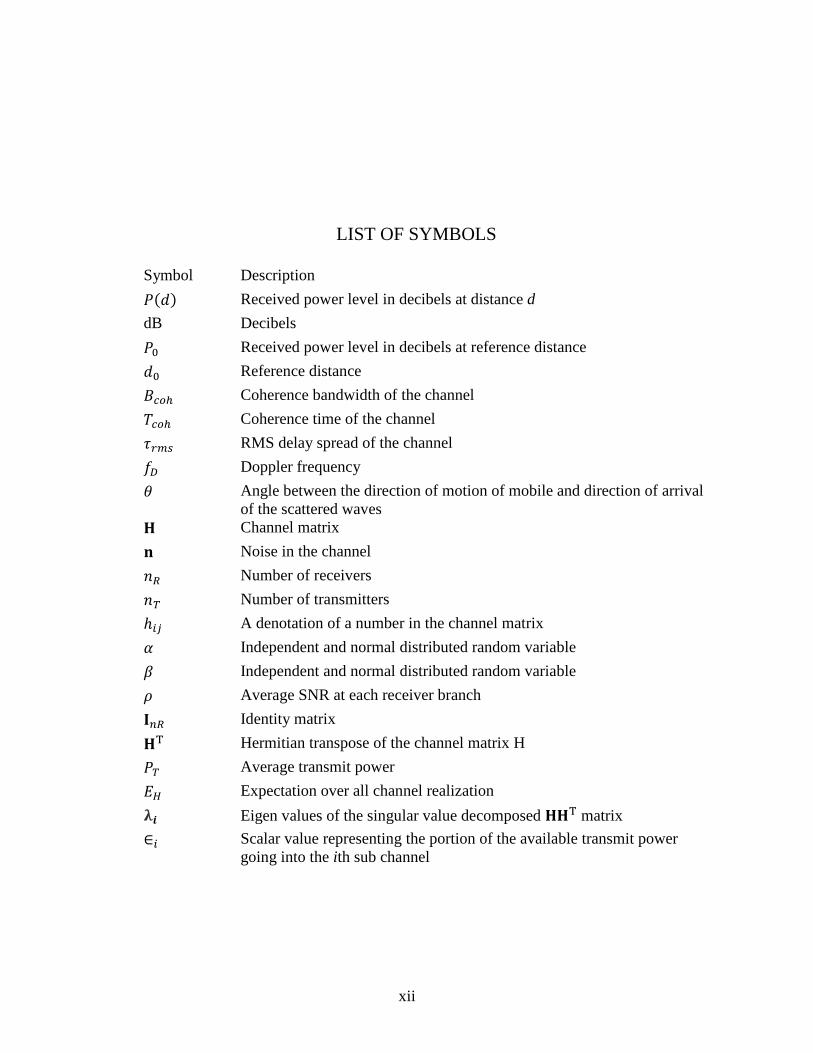
LIST OF SYMBOLS
Symbol Description
���� Received power level in decibels at distance d
dB Decibels
�� Received power level in decibels at reference distance
�� Reference distance
��� Coherence bandwidth of the channel
�� Coherence time of the channel
�� � RMS delay spread of the channel
�� Doppler frequency
� Angle between the direction of motion of mobile and direction of arrival of the scattered waves
� Channel matrix
� Noise in the channel
�� Number of receivers
�� Number of transmitters
��� A denotation of a number in the channel matrix
� Independent and normal distributed random variable
� Independent and normal distributed random variable
� Average SNR at each receiver branch
��� Identity matrix
�� Hermitian transpose of the channel matrix H
�� Average transmit power
! Expectation over all channel realization
#$ Eigen values of the singular value decomposed ��� matrix
%� Scalar value representing the portion of the available transmit power going into the ith sub channel
xiii
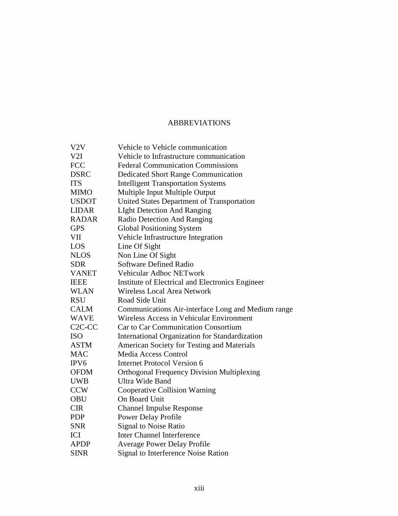
ABBREVIATIONS
V2V Vehicle to Vehicle communication V2I Vehicle to Infrastructure communication FCC Federal Communication Commissions DSRC Dedicated Short Range Communication ITS Intelligent Transportation Systems MIMO Multiple Input Multiple Output USDOT United States Department of Transportation LIDAR LIght Detection And Ranging RADAR Radio Detection And Ranging GPS Global Positioning System VII Vehicle Infrastructure Integration LOS Line Of Sight NLOS Non Line Of Sight SDR Software Defined Radio VANET Vehicular Adhoc NETwork IEEE Institute of Electrical and Electronics Engineer WLAN Wireless Local Area Network RSU Road Side Unit CALM Communications Air-interface Long and Medium range WAVE Wireless Access in Vehicular Environment C2C-CC Car to Car Communication Consortium ISO International Organization for Standardization ASTM American Society for Testing and Materials MAC Media Access Control IPV6 Internet Protocol Version 6 OFDM Orthogonal Frequency Division Multiplexing UWB Ultra Wide Band CCW Cooperative Collision Warning OBU On Board Unit CIR Channel Impulse Response PDP Power Delay Profile SNR Signal to Noise Ratio ICI Inter Channel Interference APDP Average Power Delay Profile SINR Signal to Interference Noise Ration
xiv
RMS Root Mean Square MPC Multi Path Components CSI Channel State Information SISO Single Input Single Output IPTV Internet Protocol Tele Vision STC Space Time Coding AWGN Additive White Gaussian Noise IID Independent and Identically Distributed EVD Eigen Value Decomposition SVD Singular Value Decomposition RSL Received Signal Level USRP Universal Software Radio Peripheral ARIB Association of Radio Industries and Business PER Packet Error Ratio IID Independent and Identically Distributed PHY Physical RPPP Reconfigurable Packet Routing oriented signal Processing Platforms FPGA Field Programmable Gate Array

xv
ACKNOWLEDGEMENTS
I wish to express my sincere appreciation for many individuals who have helped to complete the
research and edit this thesis. First I would like to thank my advisor, Professor Sima Noghanian
and the members of my advisory committee, Professor Reza Fazel-Rezai and Professor Saleh
Faruque, for their guidance and support during the course of this study.
Additionally, I would like to express my appreciation to North Dakota Experiment Program to
Stimulate Competitive Research (ND EPSCoR) and University of North Dakota Research
Development and Compliances for the financial support of this project.
I would also like to thank Mr. Arun Kumar for providing suggestions in developing a channel
estimator setup, Mr. Joseph Rokita, from Remcom Inc. and Mr. Esrafil Jedari, for their valuable
suggestions and comments and Dr. Arghavan Emami-Forooshani, University of British
Columbia for helping in channel capacity calculation.
Lastly, I would like to thank my family and friends for their love and support.

To my parents,
Kishor and Binita Adhikari
and my brother
Prajwal Adhikary
xvi
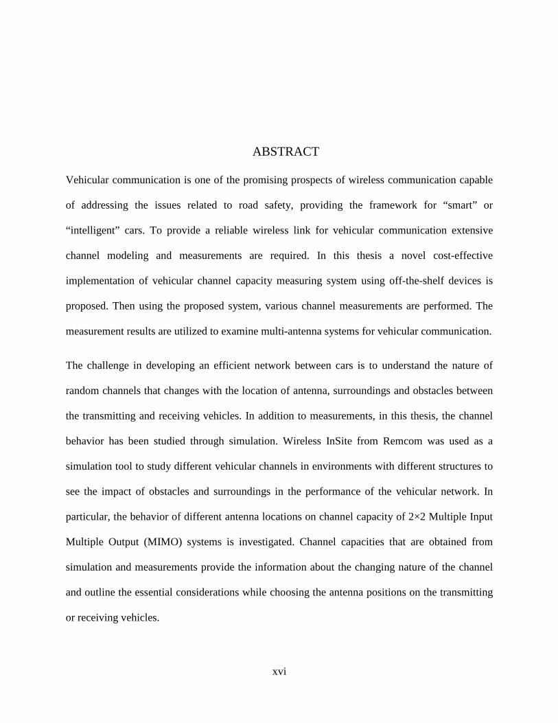
ABSTRACT
Vehicular communication is one of the promising prospects of wireless communication capable
of addressing the issues related to road safety, providing the framework for “smart” or
“intelligent” cars. To provide a reliable wireless link for vehicular communication extensive
channel modeling and measurements are required. In this thesis a novel cost-effective
implementation of vehicular channel capacity measuring system using off-the-shelf devices is
proposed. Then using the proposed system, various channel measurements are performed. The
measurement results are utilized to examine multi-antenna systems for vehicular communication.
The challenge in developing an efficient network between cars is to understand the nature of
random channels that changes with the location of antenna, surroundings and obstacles between
the transmitting and receiving vehicles. In addition to measurements, in this thesis, the channel
behavior has been studied through simulation. Wireless InSite from Remcom was used as a
simulation tool to study different vehicular channels in environments with different structures to
see the impact of obstacles and surroundings in the performance of the vehicular network. In
particular, the behavior of different antenna locations on channel capacity of 2×2 Multiple Input
Multiple Output (MIMO) systems is investigated. Channel capacities that are obtained from
simulation and measurements provide the information about the changing nature of the channel
and outline the essential considerations while choosing the antenna positions on the transmitting
or receiving vehicles.
1
CHAPTER 1
INTRODUCTION
In recent years, vehicular communication has become very important subject of study among
researchers, due to its potential to increase road-safety and reduce traffic congestion. There have
been tremendous amount of effort and investment from the government and private organizations
to develop a means for highly efficient communication between Vehicle to Vehicle (V2V) and
Vehicle to Infrastructure (V2I). Foreseeing the requirement of identical bandwidth for V2V
communication, Federal Commission Communication (FCC) has allocated 5.9 GHz band also
termed as Dedicated Short Range Communication (DSRC) to be used by Intelligent
Transportation Systems (ITS) for such communications. This thesis concentrates upon this
subject and aims to develop an efficient tool to calculate the capacity of highly random vehicular
channel for effective transmission and reception of data using Multiple Input and Multiple
Output (MIMO) technology.
1.1 Motivation
Vehicular wireless communication has been of interest to researchers in the recent years mainly
to ensure safety and mobility. As reported in [1], there are over 5.8 million vehicular crashes per
year on U.S roadways, resulting in 37,000 deaths annually. These crashes have a direct economic
burden of $230.6 billion and are one of the leading causes of death. Traffic congestion is an
$87.2 billion annual drain on the U.S economy, with 4.2 billion hours and 28 billion gallons of
fuel spent sitting in traffic, the equivalent of one-work week and three week worth of gas every

2
year. In addition to this, vehicles that are stationary, idling and traveling in a stop-and-go pattern
due to congestion emit more carbon dioxide (CO2), nitrous oxide (NOx) and methane than those
travelling in free flow conditions [1]. The necessity and demand to address this blazing issue is
the most motivating factor to contribute in some level to this field of research. There are already
numerous efforts and proposal put forwarded to end this problem. ITS program of the U.S.
Department Of Transportation (USDOT) is focusing on the integration of vehicles and road
infrastructure into intelligent systems [2]. An overview of Vehicle Infrastructure Integration
(VII) is presented in [3], which deals with the progress of this research on different part of
United States.
Various companies are investigating different solutions for ITS. Use of LIght Detection And
Ranging (LIDAR) and RADAR sensors, Global Positioning System (GPS) and digital pattern
recognition technique has already enabled Google to achieve the unprecedented benchmark [4-6]
in the form of Google CarTM. This not only represents the latest technological advancement in
this field of research but also opens the way for motor vehicle industries to invest in research to
guarantee an efficient system. One of the important challenges for such technology to work is the
Non Line Of Sight (NLOS) communication, this happens for example in the case of overtaking
by a car randomly from the traffic, or in the case of intersection where the visibility of the
passing car is obstructed by building. The Google CarTM depends on Line Of Sight (LOS)
communication between sensors and may not work properly in such cases. The MIMO systems
take advantage of NLOS situations to improve the channel quality. Therefore, these systems are
the main focus of this thesis.
This thesis discusses the behavior of the wireless random channel and its relation to different
factors like MIMO channel capacity, antenna locations, antenna height, K-Factor, phase of the
3
received signal, and multipath. To explain these factors, this thesis firstly explains the use of
simulations based on ray-tracing techniques to create a virtual environment. Later, visualizing
the appropriate height, location of antenna, Software Defined Radio (SDR) is used for building a
test bed to measure the signal strength. The obtained data is further investigated to analyze the
relation between antenna location and MIMO channel capacity.
1.2 Thesis Outline
The important previous work and ideas that motivate and drive this thesis are summarized in
Chapter 2. The literature review will introduce the reader to the subject of vehicular
communication and its standards, MIMO technique for V2V communications, capacity of such
systems and simulation and measurements in this field.
In Chapter 3 the multiple antenna systems for V2V communication is introduced. This thesis
describes a simulation technique for creating a 3 Dimensional (3D) virtual vehicular
environment. Wireless InSite™ from Remcom Inc. has been utilized to import the maps of
University of North Dakota (UND) college area and Walmart area, in Grand Forks, North
Dakota. The maps were first extracted from Google Maps. For V2V communication, two cars
are included in the simulation for transmitting and receiving ends. Multiple antennas were placed
on each antenna. The channel behavior due to change of antenna location is studied by
implementing 2×2 MIMO systems.
Chapter 4 is devoted to NLOS channels and the MIMO systems for these situations. To create a
complete NLOS scenario, an obstacle is placed between transmitting and receiving cars at
varying distances. The effect of blockage on the MIMO channel capacity is discussed in this
chapter.
4
Chapter 5 describes the test-bed and measurement scenarios and results. After the appropriate
antenna locations were figured out from the simulations, a test-bed that utilizes SDRs was used
to measure the propagation channels in real scenarios. The selected locations were the same as
those in the simulation. Multiple antenna locations were considered and by combining different
channels between antennas different MIMO systems were examined. National Instruments’
LabVIEW Software was used to control and operate the test-bed.
Chapter 6 is a discussion of future work and the conclusions we made. This chapter gives
guidelines of how this project can be extended to produce a functional benchmarking tool set.

5
CHAPTER 2
LITERATURE REVIEW
This chapter is a discussion of the research, challenges and opportunities in the field of vehicular
communication. This includes theoretical background of V2V communication, and progress
involved in developing the protocols related to it. It also focuses on the modeling and
measurement of vehicular propagation channels and introduces MIMO technique with its ability
to boost the channel capacity of the system. It further discusses relevant simulations and
measurement technique adopted to address the issue of enhancing and estimating channel
capacity for vehicular communications.
2.1 Introduction to Vehicular Communications
Vehicular communication is an ad hoc communication technology. Termed as Vehicular Ad Hoc
Network (VANET), the most popular one is working within the DSRC band. Although being in
its infancy stage, it is gaining importance for road safety and other applications. DSRC band is
75 MHz of spectrum centered at 5.9 GHz [7], which is allocated by FCC in October 1999 [8] for
ITS applications to increase traveler safety, reduce fuel consumption and pollution, and continue
to advance nation’s economy [9]. VANETs comprises V2V and V2I communications and is
based on Wireless Local Area Network (WLAN) technologies [10]. The purpose of inter-
vehicular communication (Figure 1) is to increase range and coverage of location and behavior
awareness of vehicles, which is envisaged to develop effective and highly developed pro-active
systems. The idea behind V2V communications is to make all vehicles capable to
6
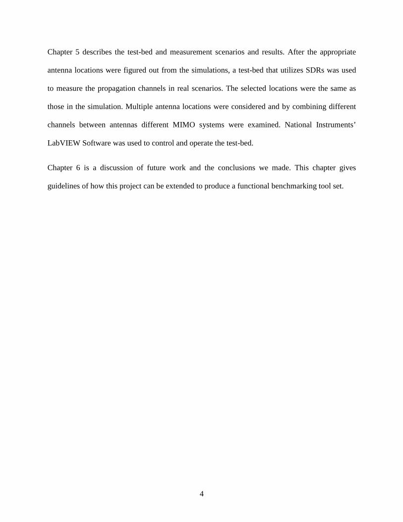
communicate information like position, speed, and heading periodically to each other in
cooperative awareness messages, in order to derive an environmental picture which could be
used for prediction of movement [11]. In recent years, the field of inter-vehicle communication
has witnessed a large increase in research and development. The key factor that has made it
possible is the wide adoption of IEEE 802.11 technologies. The availability of cellular networks
has certainly allowed voice and data communication services to drivers and passengers, but this
technology is not well suited for certain direct V2V or V2I communications.
With the availability WLAN transceivers and development in GPS since the late 1990s,
VANETs can now offer direct communication between vehicles, to and from Road-Side Units
(RSUs), which helps to exchange hazard warnings or information about the current traffic
situation with minimal latency. This has also helped to contribute to the research in the field of
inter-vehicular communication [12].
Figure 1: Inter vehicular communication [10].
The vital objectives of the research on inter-vehicle communication are to increase road safety
(which includes: reduction in the number of accidents). This is pivotal in yielding transportation
efficiency (including reduction in the number of traffic jams) which will eventually reduce the
impact of transportation on the environment (reduction in consumption of oil/gas) [1].

7
2.2 Development of V2V Communication Standards
Due to the importance of these objectives for the individual (in terms of safety) and the nation (in
terms of economy), various projects are either underway or were recently completed. Several
consortia were set up to explore the potential of VANETs. These consortia include several
constituencies, including the automotive industry, the road operators, tolling agencies, and other
service providers. These projects are funded substantially by national governments [11]. Bodies
like IEEE (Institute of Electrical and Electronics Engineers), CALM (Communications, Air-
Interface, Long and Medium Range), C2C-CC (Car to Car Communication Consortium) are
some notable ones. The architecture of Wireless Access in Vehicular Environment (WAVE),
CALM and C2C-CC is depicted in Figures 2-4 and their comparison is summarized in Table 1.
These ITS projects are really pushing the envelope to address the problem of traffic congestion
and road safety [13].
Figure 2: Wave architecture [13].

8
Figure 3: CALM architecture [13].
Figure 4: C2C-CC architecture [13].
Table 1: Comparison of C2C-CC, CALM and WAVE [13]. Parameters/Protocols C2C-CC CALM WAVE
Promotion identity Industrial consortium of
car manufactures Standard body Standard body
Focused on Car to Car multi-hop and geo-networking
Multiple media (802.11p, DSRC, W-
LAN etc.)
Only 802.11p at MAC layer for purely
emergency messaging
Physical layer DSRC and other WLAN
standards Combination of
different technologies DSRC only
Wireless technology Support for media
dependent and media independent part
Interface abstraction Only physical layers specific to 802.11p
Target applications Safety Non safety and critical Safety
Support for application types
Active safety, traffic efficiency, infotainment
Non-IP CALM aware, IPV6 CALM aware,
IPV6 legacy
Safety non-IP, non-safety IPV6
Addressing Schemes Geo-routing Mainly IP Addressing IP addressing
Routing Schemes Based on MAC protocol
(receiver based) plus IPV6
Mobile IPV6 Different channel allocation IPV6
9
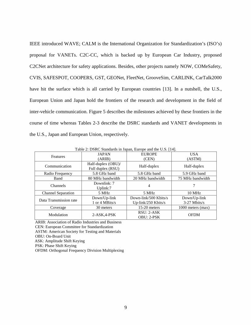
IEEE introduced WAVE; CALM is the International Organization for Standardization’s (ISO’s)
proposal for VANETs. C2C-CC, which is backed up by European Car Industry, proposed
C2CNet architecture for safety applications. Besides, other projects namely NOW, COMeSafety,
CVIS, SAFESPOT, COOPERS, GST, GEONet, FleetNet, GrooveSim, CARLINK, CarTalk2000
have hit the surface which is all carried by European countries [13]. In a nutshell, the U.S.,
European Union and Japan hold the frontiers of the research and development in the field of
inter-vehicle communication. Figure 5 describes the milestones achieved by these frontiers in the
course of time whereas Tables 2-3 describe the DSRC standards and VANET developments in
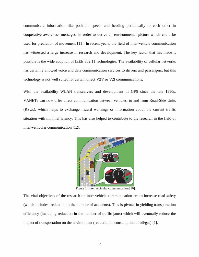
the U.S., Japan and European Union, respectively.
Table 2: DSRC Standards in Japan, Europe and the U.S. [14].
Features JAPAN (ARIB)
EUROPE (CEN)
USA (ASTM)
Communication Half-duplex (OBU)/ Full duplex (RSU)
Half-duplex Half-duplex
Radio Frequency 5.8 GHz band 5.8 GHz band 5.9 GHz band Band 80 MHz bandwidth 20 MHz bandwidth 75 MHz bandwidth
Channels Downlink: 7
Uplink:7 4 7
Channel Separation 5 MHz 5 MHz 10 MHz
Data Transmission rate Down/Up-link 1 or 4 MBits/s
Down-link/500 Kbits/s Up-link/250 Kbits/s
Down/Up-link 3-27 Mbits/s
Coverage 30 meters 15-20 meters 1000 meters (max)
Modulation 2-ASK,4-PSK RSU: 2-ASK OBU: 2-PSK
OFDM
ARIB: Association of Radio Industries and Business CEN: European Committee for Standardization ASTM: American Society for Testing and Materials OBU: On-Board Unit
ASK: Amplitude Shift Keying PSK: Phase Shift Keying OFDM: Orthogonal Frequency Division Multiplexing

10
Table 3: VANET development and trials in the U.S., Japan and European Union [14]. Country VANET development and trials
United States
Wireless Access in Vehicular Environments (2004) Intelligent Vehicle Initiative (IVI)
( 1998-2004) Vehicle Safety Communications (VSC) (2002-2004)
VSC-2 (2006-2009)
Vehicle Infrastructure Integration (VII) (2004-2009)
European Union (EU)
Car-to-Car Communications Consortium (C2C-CC) FleetNet
(2000-2003) Network On Wheels (NOW)
(2004-2005) PReVENT (2004-2008)
Cooperative Vehicles and Infrastructure Systems (CVIS)
(2006-2010) Car Talk 2000 ( 2000-2003)
Japan
Advanced Safety Vehicle Program (ASV-2) (1996-2000)
ASV-3 ( 2001-2005)
ASV-4 (2005-2007)
Demo 2000 and JARI ( Japan Automobile Research Institute)
American Society for Testing and Materials (ASTM), the standards writing group, approved the
ASTM-DSRC Standard for DSRC operations on July 10, 2003. This standard is based on IEEE
802.11a physical layer and IEEE 802.11 Media Access Control (MAC) layer and was published
as ASTM E2213-03 [7] in September 2003. FCC’s report and order, issued in February 2004,
has established service and licensing rules to govern the use of the DSRC band. In addition, it
adopted ASTM E2213-03 [7] to ensure the inter-operability and robust safety/public safety
communications among these DSRC devices nationwide. Currently, the ASTM E2213-03
standard is being migrated to the IEEE 802.11 standard [8].
11
Figure 5: Milestone is vehicular communication [10].
Unlike the fixed wireless networks, the vehicular traffic scenarios have potential barriers in form
of varying driving speeds, traffic patterns, and driving environments due to which IEEE 802.11
MAC operations suffer from significant overheads when used in vehicular scenarios. For
example, to avoid latency in vehicular safety communications, high-speed data exchanges are
required to establish a network of connections between desired nodes that may include multiple
handshakes which makes the process too complex. To illustrate this, let us take an example of a
vehicle encountering another vehicle coming in the opposite direction, the duration for possible
communication between them is extremely short [15] making it difficult to establish
communications. To meet these challenging requirements of IEEE MAC operations, the DSRC
effort of the ASTM 2313 working group migrated to IEEE 802.11 standard group which

12
renamed DSRC IEEE 802.11p as Wireless Access in Vehicular Environment (WAVE) [16].
WAVE will become a standard that can be universally adopted across the world by incorporating
DSRC into IEEE 802.11 compared to traditional DSRC. It is worth noting that IEEE 802.11p is
limited by the scope of IEEE 802.11 which strictly works at the MAC and physical (PHY) layers
(Figure 6) [17]. The operational functions and complexity related to DSRC are handled by the
upper layers of IEEE 1609 Standards. These standards define how different applications will
function in WAVE environment, based on the management activities defined in IEEE P1609.1,
the security protocols defined in IEEE P1609.2, and the network-layer protocol defined in IEEE
P1609.3.
Figure 6: WAVE, IEEE 1609, 802.11p and the OSI reference model [17].
The IEEE 1609.4 resides above 802.11p and this standard supports the operation of higher layers
without the need to deal with the physical channel access parameters. Various IEEE
1609/802.16e standards are summarized in Table 4 [14].
13
Table 4: IEEE 1609/802.16e standards [14]. IEEE Standard Description
IEEE Standard 1609
Defines the overall architecture, communication model, management structure, security mechanisms and physical access for wireless communications in the vehicular environment, the basic architectural components such as OBU, RSU and the WAVE interface [18].
IEEE Standard 1609.1-2006 Enables the interoperability of WAVE applications, describes major components of the WAVE architecture, and defines command and storage message formats [19].
IEEE Standard 1609.2-2006 Describes security services for WAVE management and application messages to prevent attacks such as eavesdropping, spoofing, alteration, and replay [20].
IEEE Standard 1609.3-2007
Specifies addressing and routing services within a WAVE system to enable secure data exchange, enables multiple stack of Upper/lower layers above/below WAVE networking services, defines WAVES short message protocol (WSMP) as an alternative to IP for WAVE applications [21].
IEEE Standard 1609.4-2006 Describes enhancements made to the 802.11 Media Access Control layers to support WAVE [22].
IEEE Standard 802.16e Enables interoperable multi-vendor broadband wireless access products [23].
2.3 V2V Communications’ Prospective Applications
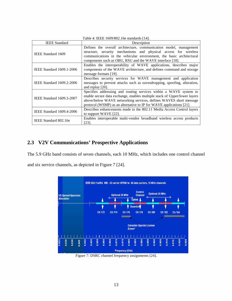
The 5.9 GHz band consists of seven channels, each 10 MHz, which includes one control channel
and six service channels, as depicted in Figure 7 [24].
Figure 7: DSRC channel frequency assignments [24].
14
DSRC, which involves V2V and V2I communications, is expected to support both safety/public
safety and non-public safety applications. However, priority is given to safety applications since
the non-public safety use of the 5.9 GHz band would be inappropriate if it leads to degrading the
performance of safety/public safety applications [8]. This is attributed to the fact that safety
applications are meant to save lives via warning drivers of an impending dangerous condition or
event in a timely manner in order to take corrective actions. Therefore, response time and
reliability are basic requirements of safety applications. DSRC PHY uses Orthogonal Frequency-
Division Multiplexing (OFDM) modulation scheme to multiplex data. Along with the successful
deployment of IEEE 802.11a WLAN services and devices in recent years, OFDM has gained
increased popularity in the wireless communication community due to its high spectral
efficiency, inherent capability to combat multi-path fading and simple transceiver design. In a
nutshell, the input data stream is divided into a set of parallel bit streams and each bit stream is
then mapped onto a set of overlapping orthogonal subcarriers for data modulation and
demodulation. All of the orthogonal subcarriers are transmitted simultaneously. By dividing a
wider spectrum into many narrow band subcarriers, a frequency selective fading channel is
converted into many flat-fading channels over each subcarrier, if the subcarrier spacing is small
compared to the channel coherence bandwidth. Thus, a simple equalization technique could be
used in the receiver to combat the inter-symbol interference [8]. As explained further in [14],
there are three different possibilities of communication configurations in ITS as depicted in
Figure 8. These include inter-vehicle, vehicle-to-roadside, and routing-based communication. In
inter-vehicle communication, a message-relaying concept is utilized where a vehicle in front
broadcasts the message, primarily the emergency events to the vehicle behind it and the vehicle
behind it does the same.

15
(a)
(b)
(c)
Figure 8: V2V communication prospective applications (a) Intervehicle communication (b) vehicle-to-roadside communication (c) routing based communication [14].
16
In V2I communication, there is periodic exchange of information between RSU and On Board
Unit (OBU) inside vehicle. RSU periodically broadcasts the message to the vehicle in its vicinity
and the vehicle updates the RSU about the information it received from the nearby RSU or
vehicle. In routing based communication, a vehicle acts as router between a vehicle in its front
and back to relay the emergency event messages. The communication inside a vehicle however
is supported by different technologies, like IEEE 802.15.1 (Bluetooth), IEEE 802.15.3 (Ultra-
wide band) and IEEE 802.15.4 (Zigbee), and it has its own importance for a reliable system.
Additional emphasis has also been given to the development of safety application (e.g. collision
avoidance, and road hazard notification) versus non-safety applications (e.g. trip planning and
infotainment), for obvious reasons. Among others, Cooperative Collision Warning (CCW) is an
important class of safety applications that target the prevention of vehicular collisions using V2V
communication [25]. The ultimate goal of CCW is to realize the concept of “360 degrees driver
situation awareness” [26-28], whereby vehicle alert driver situation of impending threats
without expensive equipment. CCW applications are generally characterized by the periodic
broadcast of short messages bearing status information (e.g. location, velocity, control settings)
that neighboring vehicles can use, for instance, to warn the driver of an impending collision [25].
Other relevant work on CCW can be found in [8, 9, 29-32]. Since enormous potential
opportunities exist for inter-vehicle communications, VANETs and ITS have to deal with the
challenge of security problems. The information being relayed in V2V communication is
definitely sometimes confidential and vulnerable too. With several tens or hundreds of
microprocessor installed in the vehicle in ITS scenarios [33], the computational process is really
complex exposing it to the possibilities of breach of the security. The attackers are classified with
17
a three dimensional approach: “insider versus outsider”, “malicious versus rational”, and “active
versus passive” as explained in [34]. Zeadally et.al [14] have classified the possibilities of
security breach as threats to availability, authenticity and confidentiality. A lot of work has also
been focused on characterizing the wireless channel used by DSRC applications.
2.4 Vehicular Propagation Path
In [35] a GPS-enabled channel sounding is presented that was used to obtain field measurement
for various speeds and LOS conditions. Channel sounding is defined as the capability to measure
the Channel Impulse Response (CIR) with any standard wireless networks and node. The
objective of processing the CIR to attain key parameters such as Power Delay Profile (PDP),
Delay Spread, Doppler Spread, Ricean K-Factor, and Signal to Noise Ratio (SNR). These
parameters are important to realize because of their impacts on security and authenticity of safety
messages being sent, especially when delay spread and Doppler spread are present, to cause Inter
Channel Interference (ICI) resulting in signal attenuation and smearing of packets within the
same channels during transmission. Averaged power at the receiver at different instants of time
is described by the Average Power Delay Profile (APDP), from which the Root Mean Square
(RMS) delay spread is evaluated [36]. The various channel metrics like pathloss, signal fading,
delay spread, Doppler spread, and angular spread has significant importance in modeling of
vehicular propagation channels which leads to the adoption of appropriate antenna system. In
[37] it is shown how path loss, Doppler spectrum and coherence time depend on both vehicle’s
speed and separation. Channel sounding is used to understand the vehicular propagation
channels. The development of efficient V2V communication systems requires understanding of
the underlying propagation channels [38]. The detailed description about vehicular propagation
channels is explained in [39]. In a wireless channel, the signal propagating from the transmitter

18
(TX) to the receiver (RX) takes several paths resulting in fading, delays, echoes and variation in
the received signal strength over time. The contributions of the various propagation paths, i.e.,
amplitudes and phases, and their respective delays define the CIR [39]. As explained in [39],
pathloss and fading determine the instantaneous Signal-To-Interference plus Noise Ratio (SINR)
which impacts the performance of the channel. For a given frequency, the received power level
in decibels (dB) is modeled as:
���� & �� ' 10�log-� . ���
/ 0 12 0 3 (1)
where d is the distance, P0 is the power level at the reference distance d0, n is the pathloss
exponent, and 12 and Y are the large-scale and small-scale fading contributions, respectively.
The RMS delay spread is calculated from APDP and gives the coherence bandwidth of the
channel. The channel is supposed to have the same transfer function or the CIR within the
coherence bandwidth. The coherence bandwidth ��� is estimated as,
��� 8 12:�� �
(2)
where, �� � is the RMS delay spread of the channel. The delay spread is more related to time
varying nature of the signal due to multipath, but it does not really deal with the time varying
nature of the channel itself. The Doppler spread and the coherence time quantifies this nature of
channel and gives the idea of how fast the channel changes and how much a pure sinusoidal
carrier is smeared over a frequency band. The coherence time of the channel can be estimated as:
�� 8 12:��
(3)
19
where ��is the Doppler spread which is a function of relative velocity of mobile, and the angle �
between the direction of motion of the mobile and direction of arrival of the scattered waves
[40].
Finally, another key quantity for the design and evaluation of vehicular antennas is the angular
spread. As discussed previously, a propagating signal generates multiple copies also termed as
MultiPath Components (MPCs) while travelling from transmitter to receiver. The large angular
spread at the receiver end supports the diversity gain whereas the small angular spread indicates
power gain by beamforming.
When we are dealing with vehicular propagation channel, the contribution of above discussed
five channel metrics hugely depends on the random and varying vehicular propagation
environment. Traditionally, propagation environment is grouped as urban, sub-urban, rural and
dense environments. Each one of these environments has its own characteristic feature like
number of lanes, width of streets, vicinity of buildings to the road, traffic density, etc. However,
when we take the movement of transmitter and receiver into considerations, cases like overtake
scenario and intersection come into play in vehicular communication. The latter two scenarios
play a pivotal role in designing and defining prototype for specific scenarios for VANETs
applications [39]. There are, however, various other application-specific scenarios for which this
classification is insufficient and where there is a need for dedicated channel characterizations
[41]. Pre-crash and post-crash warnings are a couple of examples of application specific
scenarios. Example of pre-crash warnings includes intersection collision avoidance and
cooperative merging assistance, whereas post-crash warnings are intended to facilitate traffic
flow after the occurrence of a traffic accident by broadcasting a message with the accident’s
location so that the approaching vehicles can circumvent the accident. In [42], it was investigated
20
that the success of the transmitted warning message also depends on the availability of LOS,
which has the high possibility of getting obstructed in intersection case or by a large vehicle, but
on the other hand is also capable of yielding more number of propagation paths. This helps us to
figure out two important things: first, “antenna placements” and second, “NLOS friendly
technology”. Even though the antenna design methodology for V2V antennas is already well
explored, predominantly the conventional automotive mounting concepts affect the overall
system performance metrics and significantly contribute to its limits [43, 44]. It is explained in
[45], that the “antenna placement” has a major influence on above mentioned effects, e.g., a roof-
mounted position is less likely to suffer from LOS obstruction and ultimately defines the quality
of the radio link and limits its performance metrics. Due to multipath propagation caused by
NLOS scenarios which effects all the channel metrics as discussed in [39], we need a technology
which exploits the various propagation paths caused by obstruction in LOS.
2.5 MIMO in Vehicular Communication
MIMO technology [46] promises to increase the range of communication via beamforming,
improving the reliability of communication via spatial diversity, increasing the throughput of the
network via spatial multiplexing and managing multiuser interference due to the presence of
multiple transmitting terminals [47]. MIMO, inherently has some important characteristic
features which are listed in [48, 49]. Array Gain, Diversity Gain, Multiplexing Gain, Co-Channel
Interference reduction are a few characteristics that may be improved by MIMO.
Array Gain: Due to availability of multiple antennas at both transmitter and receiver sides,
MIMO system can exploit array gain simply by coherently combining signals from different
antennas which results in increase of SNR.

21
Diversity Gain: Exploiting multiple independent fading paths either in time, frequency or space
to transmit the signal yields diversity gain of the system. At the receiver end, multiple copies of
the message signal can be attained which would eventually improve the performance and the
reliability of the system. On the transmitter side, however, correlated data can be sent through
independent fading paths exiting between transmitter and receiver.
Spatial Multiplexing Gain: Unlike diversity gain, spatial multiplexing exploits the spatial
dimension of the channel to increase the capacity for no additional power or bandwidth
expenditure. This is achieved by transmitting independent data signals simultaneously parallel on
the same frequency. The tradeoff between diversity gain and multiplexing gain is discussed in
[50].
Interference Reduction: With the knowledge of user’s Channel State Information (CSI),
multiple antennas can be used to attain the spatial signature of signal and interferes to reduce the
interference. This can be done by beamforming towards the origin of signal and nulling towards
that of interferers. Interference reduction plays a key role in complimenting spatial multiplexing
and diversity, to optimize the performance of MIMO in interference-limited dense multi-user
settings. In addition, the importance of adopting MIMO for VANETs is discussed in El-keyi et.
al [47]. The key benefits are mentioned:
MIMO versatility best matches diverse applications and scenarios: With the versatility of
MIMO system from beamforming, reducing interference to spatial multiplexing, MIMO seem to
be the best suited for the diverse scenario produced in V2V communications.
MIMO best exploits the highly dynamic V2V channel: Due to random nature of the V2V
propagation channel, traditional antenna system fails to deliver a better performance. In this
22
context, MIMO system has the potential to exploit the multipath fading creating the opportunity
for diversity and multiplexing gain.
Broadband: When it comes to communication, never-ending hunger of customers for fast
connectivity has always been a challenge. It is now quite clear that Single Input Single Output
(SISO) radios, e.g., radios based on IEEE 802.11p DSRC Standard [7], will not be enough to
support High Definition Video (HDV) with 20 Mbps requirement per stream of HD IPTV with
12-15 Mbps per stream, due to the theoretical, interference-free data rate limit of 27 Mbps
specified by the IEEE 802.11p standard. MIMO VANETs constitute a natural extension and key
part of the Mobile Broadband vision. The broadband support of MIMO brings an ample
opportunity in both safety usage and infotainment.
Reliable Communications: More than anything else, the prime objective of any system is to
provide reliable and secure communication especially in case of V2V communication, which has
its direct applications to save lives and avoid crashes on the road. MIMO technology seamlessly
lends itself to reliable communications due its inherent “diversity” benefits manifested through
well-known signal processing and pre-coding techniques at the transmitter side, beamforming
and Space-Time Coding (STC) [47] .
2.6 MIMO Capacity
It is a fact that MIMO systems offer a significant capacity gain over a traditional SISO system. In
[51] the author defines the channel capacity as a measure of how much information can be
transmitted and received with a negligible probability of error. Since the aim of this work is to
estimate the channel by calculating the channel capacity for MIMO systems, it is very important
to understand the MIMO system model and its essential parameters.
23
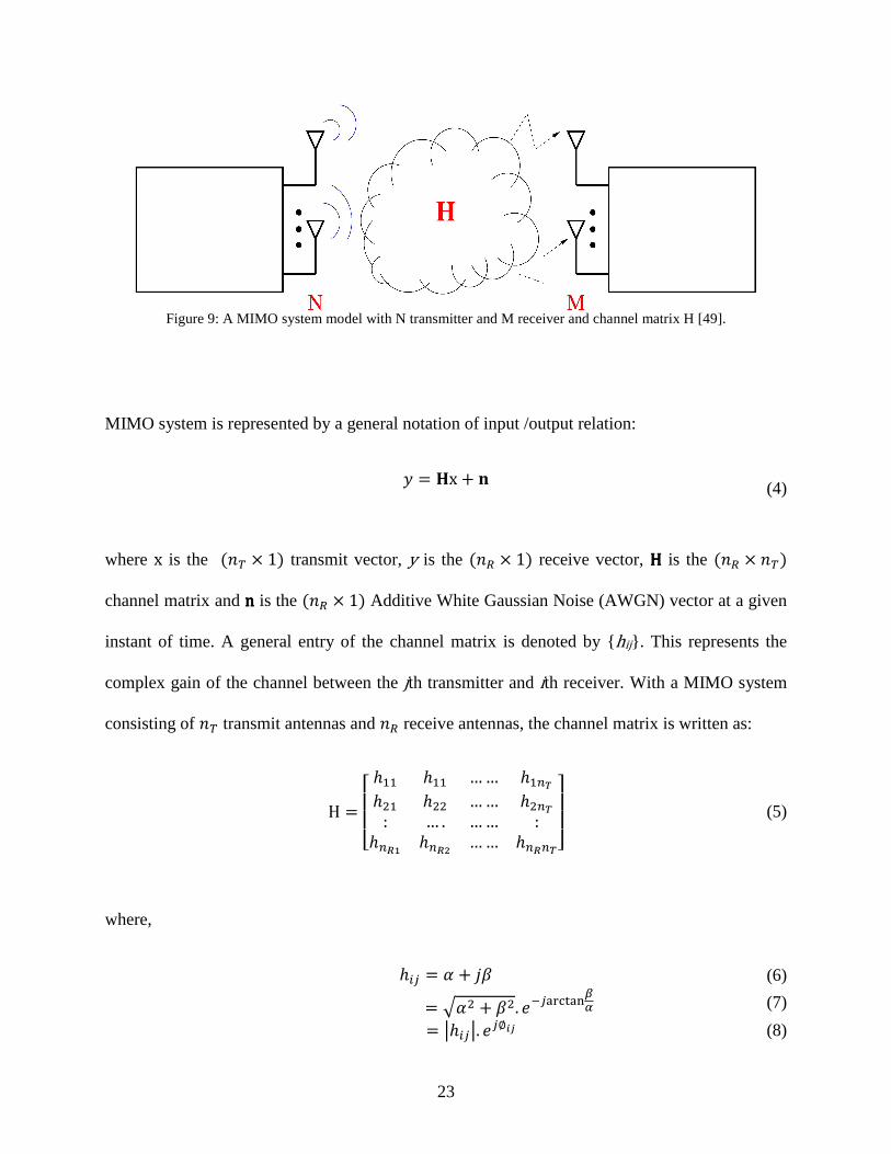
Figure 9: A MIMO system model with N transmitter and M receiver and channel matrix H [49].
MIMO system is represented by a general notation of input /output relation:
; & �x 0 �
(4)
where x is the ��� = 1� transmit vector, y is the ��� = 1� receive vector, HHHH is the ��� = ���
channel matrix and nnnn is the ��� = 1� Additive White Gaussian Noise (AWGN) vector at a given
instant of time. A general entry of the channel matrix is denoted by {hij}. This represents the
complex gain of the channel between the jth transmitter and ith receiver. With a MIMO system
consisting of �� transmit antennas and �� receive antennas, the channel matrix is written as:
H &CDDE �-- �-- … … �-�G
�H- �HH … … �H�G: … . … … :��KL ��KM … … ��K�GN
OOP (5)
where,
��� & � 0 Q� (6)
& R�H 0 �H. ST�UVWXUYZ[ (7)
& \���\. S�]^_ (8)
24
In a rich scattering environment with NLOS, the channel gains \���\ are usually Rayleigh
distributed. If � and � are independent and normal distributed random variables, then \���\ is a
random variable [51]. As explained in [52], a Rayleigh channel model have its own equation for
HHHH parameter. The Rayleigh channel model for HHHH ��� = �� channel matrix� has independent
and identically distributed (i.i.d.), complex, zero mean, unit variance entries:
f�� & Normal h0, -√Hk 0 √'1 . Normal �0, -
√H � (9)
Once we have the above descripted parameters, the ergodic (mean) capacity of a Rayleigh
complex AWGN MIMO channel can be expressed as [52, 53]
l & ! m logHndet���� 0 ��oH� ����pq (10)
This can also be written as:
l & ! m logHndet���� 0 �� ����pq (11)
where, � & rG2M is the average SNR at each receiver branch. ��� is the ��� = ��� Identity matrix.
HHHHT is the Hermitian transpose (complex conjugate transpose) of channel matrix HHHH. The above
equation of MIMO channel capacity can be further analyzed by diagonalizing the product matrix
��� either by Eigen Value Decomposition (EVD) or Singular Value Decomposition (SVD).
Our primarily interest is SVD which converts all the elements on the diagonal of ��� to zero,
except for first k elements. The number of non-zero singular matrix k equals the rank of the
channel matrix. This operation reduces the channel capacity equation to:

25
l & !m u logH .1 0 ���
λ�/qw
�x- (12)
where #$ are the eigenvalues of the the singular value decomposed ��� matrix. The maximum
capacity of a MIMO channel is reached in the unrealistic situation when each of the ��
transmitted signals is received by the same set of �� antennas without interference. It can also be
described as if each transmitted signal were received by a separate set of receiving antennas.
Also, when the channel is known at the transmitter, the maximum capacity of a MIMO channel
can be achieved by using the water-filling principle [54] on the transmit covariance matrix. The
capacity is then given by
l & !m u logH .1 0 %��
�� λ�/q
w
�x- (13)
where %� is a scalar, representing the portion of the available transmit power going into the ith
sub channel.
2.7 Simulation and Measurement
It is now clear that study of MIMO systems for vehicular communications is an important part of
establishing such systems. This section is dedicated to the study of the literature about the work
that has been done in the related field. There are various publications on this topic including the
estimation of the channel capacity or channel parameters using both simulations [55-57] and
measurements [35, 37, 38, 41-43, 58-73]. The work presented in [57] is based on ray-tracing
simulation of the channel.
26
We also chose to use a commercially available ray-tracing software, Wireless-InSite® from
Remcom [74]. This tool is capable of simulating a realistic 3D traffic models that can be used to
find optimal configurations. Parameters like Received Signal Level (RSL), PDP, and delay
spread, Doppler spread, and Ricean K-Factor can be evaluated and represented in graphically.
Multipath travelled by electromagnetic waves can also be studies as explained in [75] which can
be useful to calculate the channel capacity and analyze it with different antenna configurations
and placement.
For the measurement of channel parameters in real time scenarios we designed and implemented
a test-bed using SDRs. SDRs were selected due to their low cost and ease of implementation.
Different scopes of using SDRs are discussed on [68-73]. In [68], Universal Software Radio
Peripheral (USRP) modules, the widely used and documented off-the-shelf SDR kits, were used
to find the range of reception between RSU and OBU, for ARIB STD-T75 standard (and
equivalent WAVE standard used in Japan, Table 2). Packet Error Ratio (PER) and channel
power was measured in this study using USRP modules. In [70, 71], a SDR simulator was
designed for testing various baseband transceivers for both DSRC and Ultra Wide Band (UWB)
communications. The system accounts for slow and fast fading as well as frequency selective
fading. It includes two types of waveform codes, Doppler spread and delay spread. The software
processing includes modules that simulate a fading channel generator, interpolator, register bank
and multipath signal generator. The Doppler spectra calculated by the simulator and obtained by
measurements were compared for a slower speeds and lower frequency (2.4 GHz and were up
scaled to faster speeds and 5.9 GHz) data and the spectra are found to be similar. In [69] another
use of USRP modules is shown, where the IEEE 1609.x standard is implemented on the USRP
radio modules. Using GNU Radio (that is included in the USRP modules) gives an easy way to

27
manage complex WAVE layer stacks. A low bit rate version of the PHY layer was implemented,
as higher bit rate version as stipulated by the standard was not possible due to communication
limitations between processing Personal Computer (PC) and USRP. The USRP modules used to
implement PHY layer work at 2.4 GHz. In [72], the authors demonstrate an in-house prototype
model of the OMIcar, a model car with a sensor cluster for autonomous driving and equipped
with SDR and various sensors and reader. In the research sponsored by Toyota, [73]
Reconfigurable Packet Routing-Oriented Signal Processing Platforms (RPPP) is proposed to
dynamically adapt a Field Programmable Gate Array (FPGA) based SDR which has multi-
channel capabilities.
2.8 Summary
In this chapter a brief literature review of V2V and V2I communication and standards was given.
The importance of channel modeling and MIMO channel to exploit maximum channel capacity
was discussed and a few examples of pervious work on channel simulation and measurements
were reviewed.
28
CHAPTER 3
MULTIPLE ANTENNA SYSTEMS FOR VEHICLE TO
VEHICLE COMMUNICATIONS
In this chapter we study the channel behavior and particularly the use of MIMO systems in V2V
communication. The study performed in this chapter is entirely based on simulation. First the
method of creating a 3D virtual vehicular environment is explained. Wireless InSite™ from
Remcom Inc. has been utilized for all the simulations. Two major scenarios were considered.
The first scenario was a location selected on campus at the University of North Dakota (UND),
in Grand Forks, North Dakota (referred to as college area). The second scenario was a location
close to commercial and residential buildings in the vicinity of Walmart, Grand Forks, North
Dakota (referred to as Walmart area). The exact building locations and dimensions were
imported from Google Maps. In this chapter our focus is on V2V communication without any
blocking obstacles. Although, due to antenna locations, some channels did not have LOS (NLOS
channel), these scenarios did not happen because of blocking vehicle or building obstruction.
The car located in the back was considered to be transmitting end and the front car was
considered to be receiving end. Multiple antennas were placed on both cars. The behavior of
different locations of antennas on the channel capacity for different possible 2×2 MIMO setups
was studied.
29
3.1 Methodology
Wireless InSite is a ray-tracing electromagnetic simulation tool for predicting the effects of
buildings and terrain on the propagation of electromagnetic waves. It predicts how the locations
of the transmitters and receivers within an area affect the signal strength. It models the physical
characteristics of the rough terrain and urban building features, performs the electromagnetic
calculations, and then evaluates the signal propagation characteristics [3]. The frequency range
opted for our simulation was from 5.855 to 5.925 GHz which is allocated to DSRC and WAVE
channels.
3.1.1 System Set Up
We used half-wave dipole antennas at both TX and RX ends. The systems work around 5.9 GHz
(wavelength of 0.053m) center frequency with 10 MHz bandwidth. There were 15 dipole
antennas mounted on the top, front and rear sides of the cars. The antennas were overlaid in 5
columns and 3 rows. The distance (front to back) between two cars was 15 meters. The
transmitting power in both the scenarios was selected at 0 dBm.
Figure 10 gives the overview of the antennas’ layout on the cars. Each column is named as a
“route” in Wireless InSite, e.g. antennas 1, 2 and 3 correspond to route 1. Table 5 summarizes
the spacing between each two antennas and center-to-center distances between each pair of
routes. The spacing between elements in each route was uniform.

30
Figure 10: Layout of antenna positions and their assigned numbers in transmitting and receiving vehicles.
Table 5: Spacing between antennas.
Antenna No./Route No. Spacing (m) Spacing (wavelength)
1-2, 2-3 (Route 1) 0.50 9.43
4-5, 5-6 (Route 2) 0.35 6.60
7-8, 8-9 (Route 3) 0.35 6.60
10-11, 11-12 (Route 4) 0.35 6.60
13-14, 14-15 (Route 5) 0.50 9.43
Route 1 and Route 2 1.07 20.19
Route 2 and Route 3 0.40 7.55
Route 3 and Route 4 0.35 6.60
Route 4 and Route 5 1.60 30.19
3.1.2 Environment Modeling
In the simulation, we used materials like bricks for the building and asphalt for the road. Also,
wood is used for trees. The details of material selection for each scenario and assumed heights
are summarized in Tables 6 and 7. The height of antenna element depends on the surface on

31
which it is mounted. Antennas at the rear or front sides of the car have heights of 0.95 m (0.91 in
case of college area), which is smaller in comparison to those mounted on the roof at 1.35 m. In
Section 3.2 the impact of height on system performance is discussed. Google Maps was used to
delineate the exact location of buildings. The image of each scenario was imported into Wireless
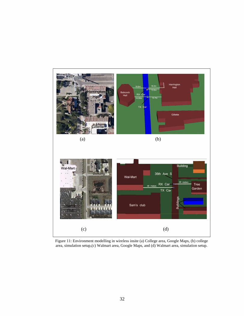
InSite and the environmental set up was built. Figure 11 show the maps extracted from Google
Maps and their implementation in simulation set up and the distances between each car and the
closest interferers are given. The effect of this difference in the performance of the system will
be discussed in Section 3.2.
Table 6: Material selection for simulation in the college area. Feature Description Type Height (m)
Terrain Wet earth DHS 0.00
Babcock Hall Brick OLD 6.00
Harrington Hall Brick OLD 6.00
Gillette Brick OLD 6.00
Road Asphalt DHS 0.10
Cars PVC, Metal,
Glass OLD, PEC,
OLD 1.35
PVC: PolyVinyl Chloride, DHS: Dielectric Half-Space, OLD: One-Layer Dielectric, PEC: Prefect Electric Conductor
Table 7: Material selection in the Walmart area.
Feature Description Type Height (m)
Terrain Wet Soil DHS 0.00
Walmart Brick OLD 9.00
Sam’s-Club Brick OLD 9.00
Buildings
1,2,3 Brick OLD 6.00
Road Asphalt DHS 0.10
Cars PVC, Metal,
Glass OLD, PEC,
OLD 1.35
Tree Garden
Wood OLD 3.00
PVC: PolyVinyl Chloride, DHS: Dielectric Half-Space, OLD: One-Layer Dielectric, PEC: Prefect Electric Conductor
32
(a) (b)
(c) (d)
Figure 11: Environment modelling in wireless insite (a) College area, Google Maps, (b) college area, simulation setup,(c) Walmart area, Google Maps, and (d) Walmart area, simulation setup.
33
3.1.3 Implementing MIMO System
The application of MIMO systems has primarily been in the case of NLOS scenarios which are
mainly due to blockages in the transmission of signals. In NLOS scenarios, signal travels through
multipath and arrives at the receiver at different angles. This gives rise to channel diversity that
can be used in MIMO systems to improve the channel capacity [39]. In Figure 12, the signal has
to reach from antennas on the TX car to the antennas on the RX car, which might or might not be
in the LOS. In such cases, paths followed by the signal takes either the direct path or the
multipath due to reflection from the ground, as shown in Figure 12 (a), or from the surrounding
obstacles (building and trees in our case), as shown in Figure 12 (b). The availability of multiple
antenna elements at both ends allows us to choose desired antenna location to form a MIMO
system. We have chosen various possible 2×2 MIMO systems (2 transmitting antennas and 2
receiving antennas) and compared them in terms of their capacities. The channel capacity of the
MIMO system is calculated by:
l & logHndet���K 0 ���
����p (14)
where, ρ is the receiver SNR, HHHH is the channel matrix, I nR is the identity matrix, and HHHHT is the
Hermitian or conjugate transpose of HHHH. All matrices have the size of nT×nR where nT is the
number of transmitter antennas and nR is the number of receiver antennas [76].
The occurrence of the multipath depends on the vicinity of the interfering object. The closer the
obstacle is, the greater the multipath is, as shown in Figure 12 (b) and (c). While the paths with
maximum power in both scenarios were similar, the number of multipath elements in the

34
Walmart area is less than that in the college area. This is mainly due to the differences in the
distances between the cars and the closest objects.
3.2 Results and Discussions
Tables 8 and 9 show the relation between received power level of antennas and their locations
with respect to antenna positions in the college area, whereas Tables 10 and 11 show the same
for the Walmart area. For antennas located on the rooftop, the received powers by antennas are
very similar (Tables 8 and 10). However, the received power for antennas located at the rear or
(a) (b)
(c)
Figure 12: Path travelled by the wave in college and Walmart area (a) Direct path and multipath, (b) multipath in college area, and (c) multipath in Walmart area.
35
front positions vary. From Tables 9 and 11, for example, RX 1 accumulates highest power being
the closest to TX 15, whereas RX 15 receives the least power.
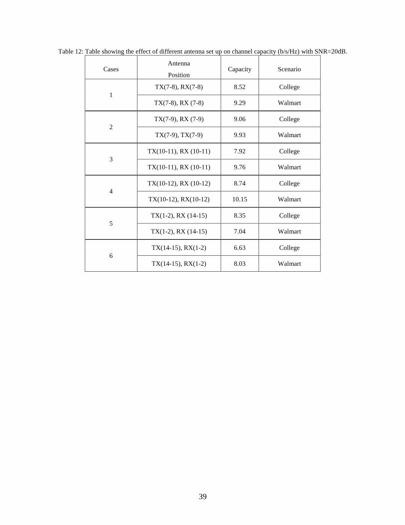
Table 12 shows the capacities of six different antenna positions in the TX and RX car for both
scenarios yielding different capacity values. These positions were chosen from 225 different
possibilities. We identified these 6 cases as the most revealing ones. The capacities of the MIMO
systems were calculated using (14). The calculated capacity is compared with the maximum
capacity calculated using a 2×2 identity matrix and the average Rayleigh channel capacity. For
mean Rayleigh capacity for a 2×2 MIMO over 1000 iterations of AWGN channels were
generated and the average value of the channel capacity was taken [52]. The capacity for 2×2
identity matrix channel and the 2×2 Rayleigh channel for 20dB SNR are 10.30 and 7.90
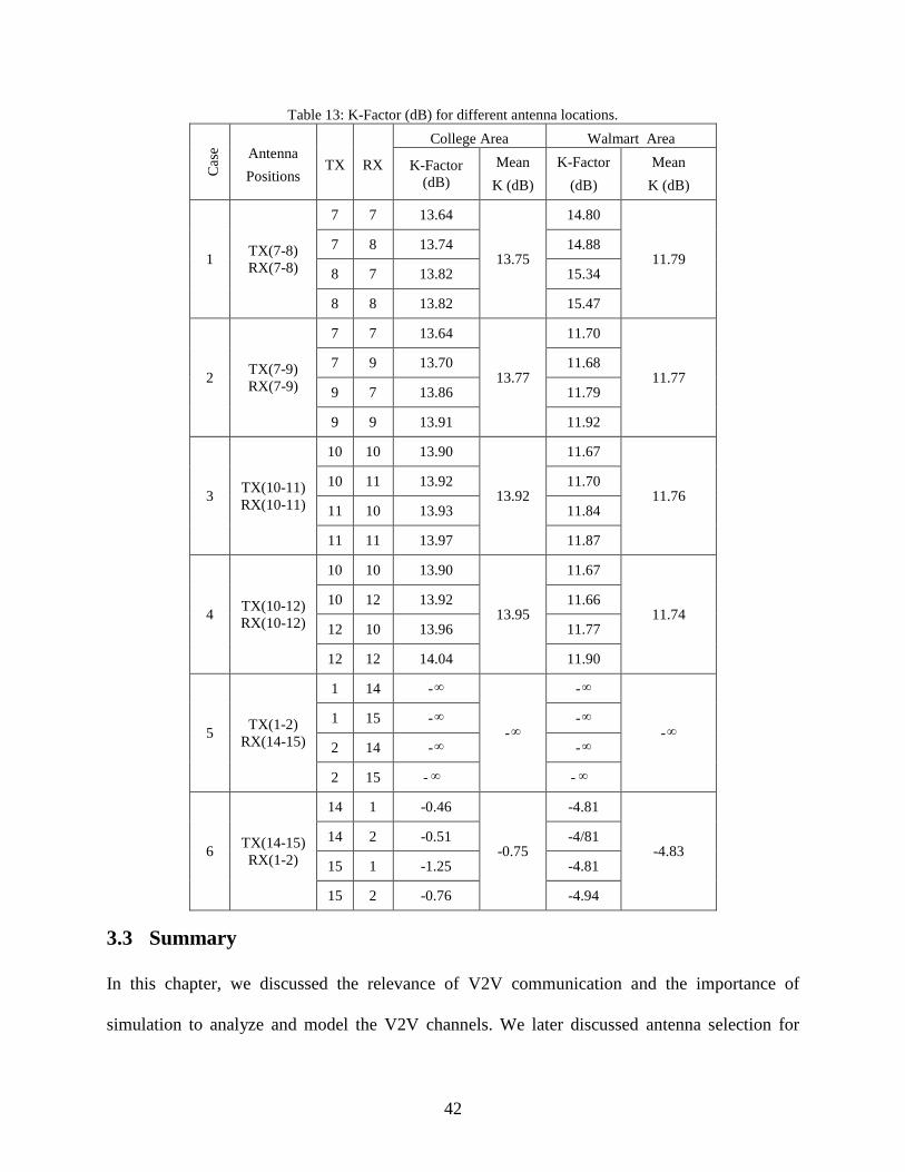
bits/s/Hz, respectively. Table 12 should be viewed in conjunction with Table 13 that shows the
Ricean K-Factor for the 6 chosen cases. Ricean K-Factor is defined as the power ratio of the
LOS component to the diffused component [77]. The higher values of K-Factor imply that direct
path is stronger compared to the multipaths’ power. Hence, the K-Factor has direct effects on the
performance of MIMO systems. Small K-Factor values are associated with richer multi-path
environments and should provide higher capacities [78]. “Mean (K)” in Table 13 represents the
average of K-Factors produced in any selected cases by taking an average of K-Factors over the
four possible channels.
The results for the first 4 cases are easy to comprehend and important to understand. Channel
capacities in the Walmart area are generally greater than those in the college area, also the K-
Factor in the Walmart area in all 4 cases is less than those of the college area. The antenna
spacing for both scenarios in the first 4 cases are presented in Table 5. Cases 2 and 4 yield
maximal capacity values as the spacing between antennas is 0.70m (13.20λ) as compared to the
36
spacing between antennas in Cases 1 and 3, i.e. 0.35m (6.60λ), which is similar to many MIMO
systems [79]. Results of the K-Factor and capacities in Cases 5 and 6 are riveting and may draw
any researcher’s attention. First, despite having the same K-Factor value for NLOS condition of
Case 5, the capacity of the college area is higher than that of the Walmart area. In Case 5,
transmitters are in the rear of the car with antenna height 0.95m, which is clearly obstructed by
glass that extends to the roof at the height of 1.35m. Hence, the entire signal are either reflected
back or scattered before reaching the receiver in front of the RX car. This shows the importance
of proximity of the obstacle to yield more multipaths. As shown in Figures. 11 (b) and (d), the
obstacles in the college area are closer to the TX and RX cars compared to the Walmart area,
which eventually boosts up the channel capacity of college area for that antenna position. Also,
the K-Factor of both areas of Case 5 are 0 (-∞ in dB) suggesting a rich scattering environment
with NLOS, and the HHHH matrix similar to Rayleigh fading channel [6]. Their respective capacities
are also around the mean Rayleigh capacity. However, the capacities are lower than Cases 1 and
3, which have similar antenna spacing. It should be noted that the value of K-factor in Case 6 for
both scenarios is very low compared to the first 4 Cases, despite being the most prominent LOS
position. In an attempt to investigate the reason behind this, we found that the height of the
antenna element plays a crucial role. Initially, the “Mean (K)” for the Walmart area for Case 6
was 0, which increased to 0.33 when we increased the antenna height merely by 0.05m.
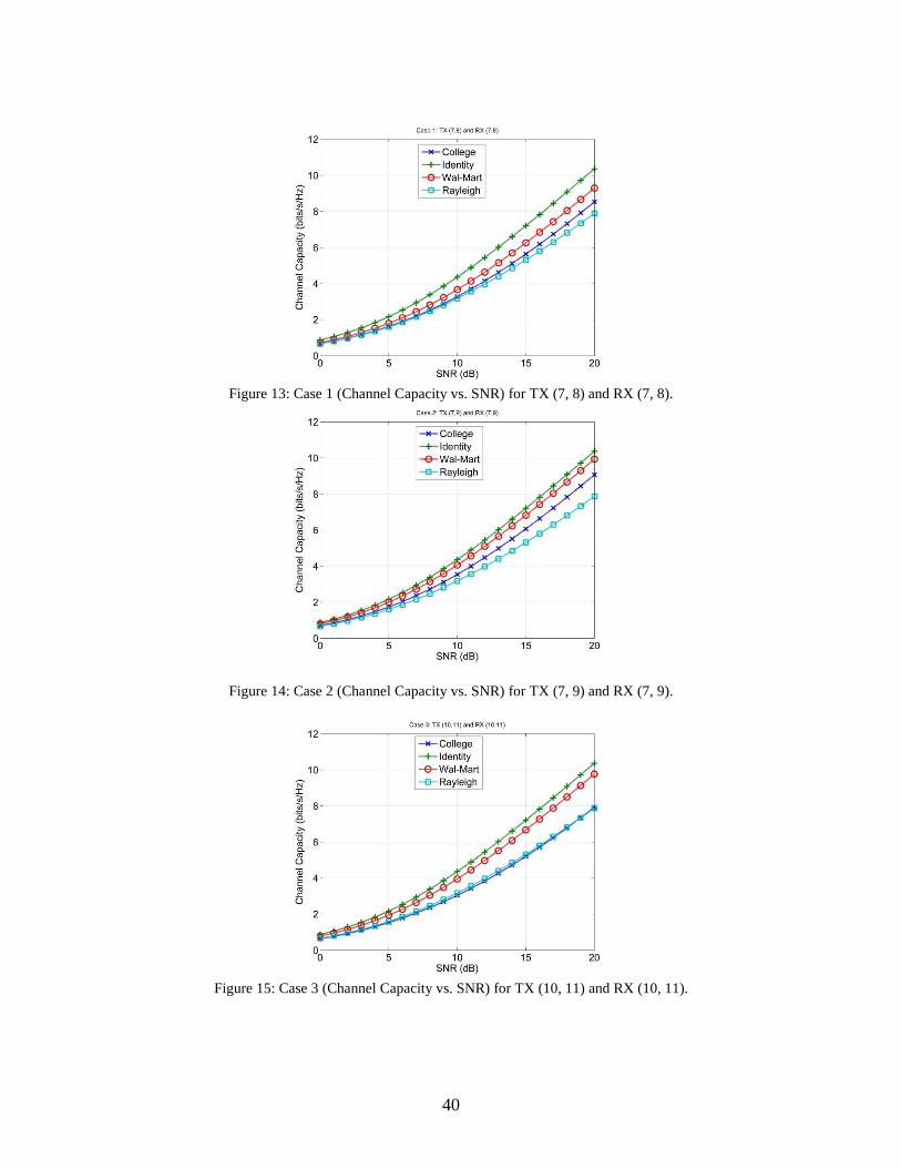
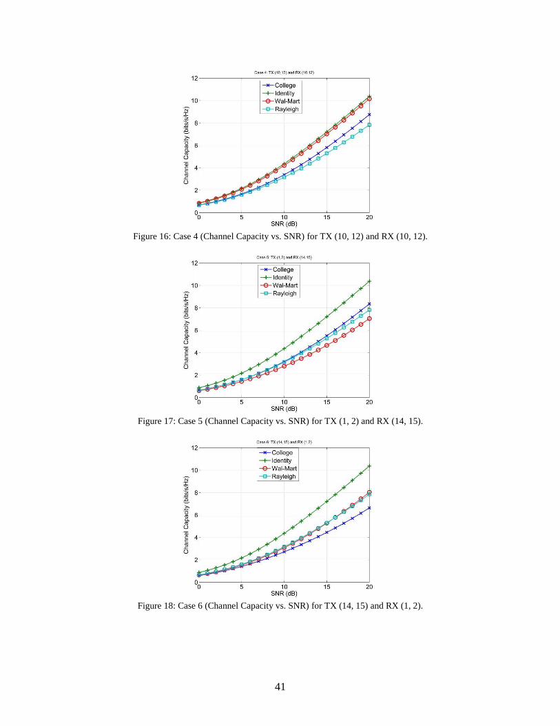
Figures 13 through 18 show the capacity of 2×2 MIMO systems with respect to SNR ranging
from 0 to 20 dB. These figures correspond to the antenna position and the scenarios described in
Table 12.

37
Table 8: Power received by different receivers on rooftop with respect to the corresponding transmitter antenna for college area.
TX
Received Power by Receiver Number (dBm)
7 8 9 10 11 12
7 -65.56 -69.89 -67.24 -68.19 -66.83 -65.75
8 -66.41 -66.27 -66.35 -66.23 -65.42 -66.45
9 -68.29 -67.99 -67.71 -68.12 -68.42 -69.65
10 -65.73 -68.48 -65.80 -68.68 -67.26 -64.77
11 -68.73 -66.74 -64.61 -65.20 -66.53 -66.08
12 -67.64 -67.16 -67.48 -68.53 -69.36 -68.00
Table 9: Power received by different receivers on rear and back with respect to the corresponding transmitter
antenna for college area.
TX
Received Power by Receiver Number (dBm)
1 2 3 13 14 15
1 -78.56 -84.42 -85.08 -89.69 -104.76 -81.94
2 -82.55 -80.77 -76.05 -89.81 -86.73 -95.46
3 -70.91 -78.17 -74.48 -100.75 -94.19 -92.11
13 -66.97 -65.38 -63.59 -84.14 -80.79 -76.08
14 -64.34 -67.35 -59.09 -81.55 -82.50 -86.50
15 -58.45 -65.87 -60.32 -84.55 -77.28 -88.91

38
Table 10: Power received by different receivers on roof top with respect to the corresponding transmitter antenna for
Walmart area.
TX
Received Power by Receiver Number (dBm)
7 8 9 10 11 12
7 -80.5 -85.16 -83.10 -72.78 -76.16 -79.02
8 -81.18 -76.84 -99.76 -83.51 -84.72 -82.49
9 -83.74 -84.43 -84.97 -81.15 -86.38 -97.73
10 -61.85 -69.38 -67.49 -99.83 -99.96 -100.09
11 -61.41 -63.53 -65.64 -84.28 -84.26 -85.76
12 -62.49 -72.05 -75.61 -89.98 -82.95 -85.17
Table 11: Power received by different receivers on rear and back with respect to the corresponding transmitter antenna for Walmart area.
TX
Received Power by Receiver Number (dBm)
1 2 3 13 14 15
1 -71.41 -67.77 -69.50 -71.18 -70.20 -67.19
2 -67.79 -71.82 -69.27 -70.53 -68.96 -70.19
3 -69.59 -69.25 -69.66 -67.27 -70.15 -71.39
13 -70.06 -68.09 -68.02 -67.03 -72.78 -68.87
14 -68.06 -69.93 -68.09 -72.87 -67.52 -70.64
15 -68.08 -67.95 -72.53 -69.10 -70.50 -66.90
39
Table 12: Table showing the effect of different antenna set up on channel capacity (b/s/Hz) with SNR=20dB.
Cases Antenna
Position Capacity Scenario
1 TX(7-8), RX(7-8) 8.52 College
TX(7-8), RX (7-8) 9.29 Walmart
2 TX(7-9), RX (7-9) 9.06 College
TX(7-9), TX(7-9) 9.93 Walmart
3 TX(10-11), RX (10-11) 7.92 College
TX(10-11), RX (10-11) 9.76 Walmart
4 TX(10-12), RX (10-12) 8.74 College
TX(10-12), RX(10-12) 10.15 Walmart
5 TX(1-2), RX (14-15) 8.35 College
TX(1-2), RX (14-15) 7.04 Walmart
6 TX(14-15), RX(1-2) 6.63 College
TX(14-15), RX(1-2) 8.03 Walmart
40
Figure 13: Case 1 (Channel Capacity vs. SNR) for TX (7, 8) and RX (7, 8).
Figure 14: Case 2 (Channel Capacity vs. SNR) for TX (7, 9) and RX (7, 9).
Figure 15: Case 3 (Channel Capacity vs. SNR) for TX (10, 11) and RX (10, 11).
41
Figure 16: Case 4 (Channel Capacity vs. SNR) for TX (10, 12) and RX (10, 12).
Figure 17: Case 5 (Channel Capacity vs. SNR) for TX (1, 2) and RX (14, 15).
Figure 18: Case 6 (Channel Capacity vs. SNR) for TX (14, 15) and RX (1, 2).
42
Table 13: K-Factor (dB) for different antenna locations.
Cas
e
Antenna
Positions TX RX
College Area Walmart Area
K-Factor (dB)
Mean
K (dB)
K-Factor
(dB)
Mean
K (dB)
1 TX(7-8) RX(7-8)
7 7 13.64
13.75
14.80
11.79 7 8 13.74 14.88
8 7 13.82 15.34
8 8 13.82 15.47
2 TX(7-9) RX(7-9)
7 7 13.64
13.77
11.70
11.77 7 9 13.70 11.68
9 7 13.86 11.79
9 9 13.91 11.92
3 TX(10-11) RX(10-11)
10 10 13.90
13.92
11.67
11.76 10 11 13.92 11.70
11 10 13.93 11.84
11 11 13.97 11.87
4 TX(10-12) RX(10-12)
10 10 13.90
13.95
11.67
11.74 10 12 13.92 11.66
12 10 13.96 11.77
12 12 14.04 11.90
5 TX(1-2)
RX(14-15)
1 14 -∞
-∞
-∞
-∞ 1 15 -∞ -∞
2 14 -∞ -∞
2 15 -∞ -∞
6 TX(14-15) RX(1-2)
14 1 -0.46
-0.75
-4.81
-4.83 14 2 -0.51 -4/81
15 1 -1.25 -4.81
15 2 -0.76 -4.94
3.3 Summary
In this chapter, we discussed the relevance of V2V communication and the importance of
simulation to analyze and model the V2V channels. We later discussed antenna selection for

43
multiple antenna systems and adopting the MIMO system. We conclude, although in general, the
MIMO capacity increases with SNR and antenna spacing, in V2V communication the location of
antenna also plays an important role. We observed the occurrences of maximum capacity and
increase in capacity by increasing the antenna spacing happens mostly when antennas are located
on the rooftop. Also, the antenna height proved to be the essential factor. The relation of the K-
Factor to the calculated channel capacity showed that the capability of MIMO system increased
for lower K-Factor as long the antenna height was the same. However, lower K-Factor for lower
heights did not show better capacity in compared to higher K-Factor for antenna elements at
higher positions. This raises the question if the vehicular channels follow Rayleigh or Ricean
fading channels.

44
CHAPTER 4
EFFECTS OF BLOCKAGE ON THE MIMO CAPACITY FOR DSRC
CHANNELS
The application of vehicular communication depends on its efficiency to address the different
possible scenario. As discussed previously, DSRC for V2V communication is widely
investigated to ensure traffic safety and reduce traffic congestion. In Chapter 3, we investigated
the channel capacity for MIMO systems through simulation, considering different antenna
locations and heights through simulation of such environments. In this chapter, we will discuss
the effect of blockage in similar setups. Additionally, we will compare these cases with the non-
blockage cases that were presented in Chapter 3.
4.1 Introduction
DSRC [7] is an automotive communication protocol that is popular for its potential application
like Lane Changing Warning (LCW), Forward Collision Warning (FCW) in ensuring traffic
safety and reducing traffic accidents. The major challenge in developing such application to
provide a 360 degrees view of traffic status is to overcome the hurdle provided by the obstacles
in form of buildings (in intersection), heavy vehicles (in case of overtaking), generally
categorized as NLOS scenarios [80]. In this chapter, we have used a vehicle as an obstacle
between two other vehicles (between the transmitting and receiving ends). Antennas were placed
at various locations on the vehicles’ bodies. A total of 15 antennas were spread on the rear,
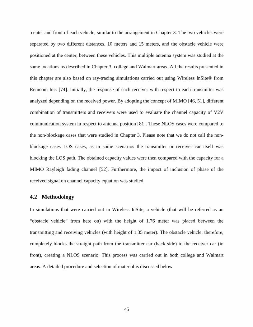
45
center and front of each vehicle, similar to the arrangement in Chapter 3. The two vehicles were
separated by two different distances, 10 meters and 15 meters, and the obstacle vehicle were
positioned at the center, between these vehicles. This multiple antenna system was studied at the
same locations as described in Chapter 3, college and Walmart areas. All the results presented in
this chapter are also based on ray-tracing simulations carried out using Wireless InSite® from
Remcom Inc. [74]. Initially, the response of each receiver with respect to each transmitter was
analyzed depending on the received power. By adopting the concept of MIMO [46, 51], different
combination of transmitters and receivers were used to evaluate the channel capacity of V2V
communication system in respect to antenna position [81]. These NLOS cases were compared to
the non-blockage cases that were studied in Chapter 3. Please note that we do not call the non-
blockage cases LOS cases, as in some scenarios the transmitter or receiver car itself was
blocking the LOS path. The obtained capacity values were then compared with the capacity for a
MIMO Rayleigh fading channel [52]. Furthermore, the impact of inclusion of phase of the
received signal on channel capacity equation was studied.
4.2 Methodology
In simulations that were carried out in Wireless InSite, a vehicle (that will be referred as an
“obstacle vehicle” from here on) with the height of 1.76 meter was placed between the
transmitting and receiving vehicles (with height of 1.35 meter). The obstacle vehicle, therefore,
completely blocks the straight path from the transmitter car (back side) to the receiver car (in
front), creating a NLOS scenario. This process was carried out in both college and Walmart
areas. A detailed procedure and selection of material is discussed below.
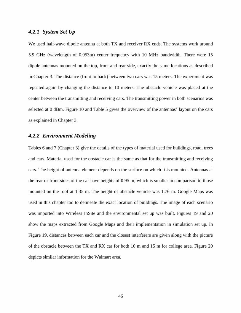
46
4.2.1 System Set Up
We used half-wave dipole antenna at both TX and receiver RX ends. The systems work around
5.9 GHz (wavelength of 0.053m) center frequency with 10 MHz bandwidth. There were 15
dipole antennas mounted on the top, front and rear side, exactly the same locations as described
in Chapter 3. The distance (front to back) between two cars was 15 meters. The experiment was
repeated again by changing the distance to 10 meters. The obstacle vehicle was placed at the
center between the transmitting and receiving cars. The transmitting power in both scenarios was
selected at 0 dBm. Figure 10 and Table 5 gives the overview of the antennas’ layout on the cars
as explained in Chapter 3.
4.2.2 Environment Modeling
Tables 6 and 7 (Chapter 3) give the details of the types of material used for buildings, road, trees
and cars. Material used for the obstacle car is the same as that for the transmitting and receiving
cars. The height of antenna element depends on the surface on which it is mounted. Antennas at
the rear or front sides of the car have heights of 0.95 m, which is smaller in comparison to those
mounted on the roof at 1.35 m. The height of obstacle vehicle was 1.76 m. Google Maps was
used in this chapter too to delineate the exact location of buildings. The image of each scenario
was imported into Wireless InSite and the environmental set up was built. Figures 19 and 20
show the maps extracted from Google Maps and their implementation in simulation set up. In
Figure 19, distances between each car and the closest interferers are given along with the picture
of the obstacle between the TX and RX car for both 10 m and 15 m for college area. Figure 20
depicts similar information for the Walmart area.

47
Figure 19: Distance between cars and the surrounding obstacles (college area).
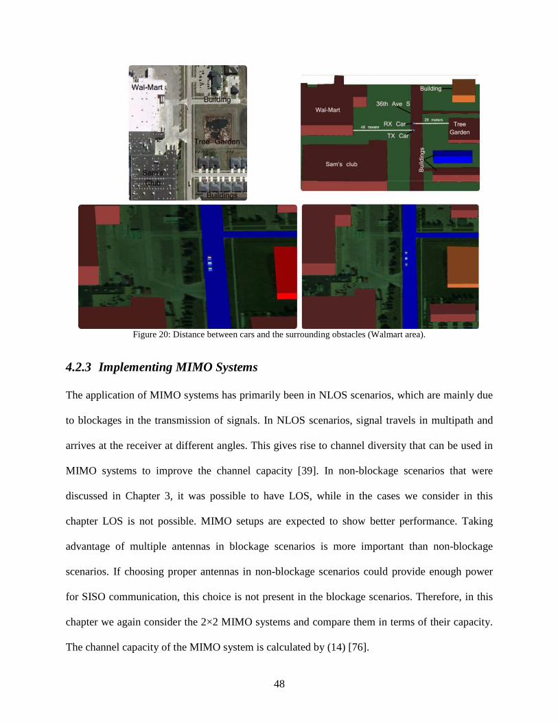
48
Figure 20: Distance between cars and the surrounding obstacles (Walmart area).
4.2.3 Implementing MIMO Systems
The application of MIMO systems has primarily been in NLOS scenarios, which are mainly due
to blockages in the transmission of signals. In NLOS scenarios, signal travels in multipath and
arrives at the receiver at different angles. This gives rise to channel diversity that can be used in
MIMO systems to improve the channel capacity [39]. In non-blockage scenarios that were
discussed in Chapter 3, it was possible to have LOS, while in the cases we consider in this
chapter LOS is not possible. MIMO setups are expected to show better performance. Taking
advantage of multiple antennas in blockage scenarios is more important than non-blockage
scenarios. If choosing proper antennas in non-blockage scenarios could provide enough power
for SISO communication, this choice is not present in the blockage scenarios. Therefore, in this
chapter we again consider the 2×2 MIMO systems and compare them in terms of their capacity.
The channel capacity of the MIMO system is calculated by (14) [76].
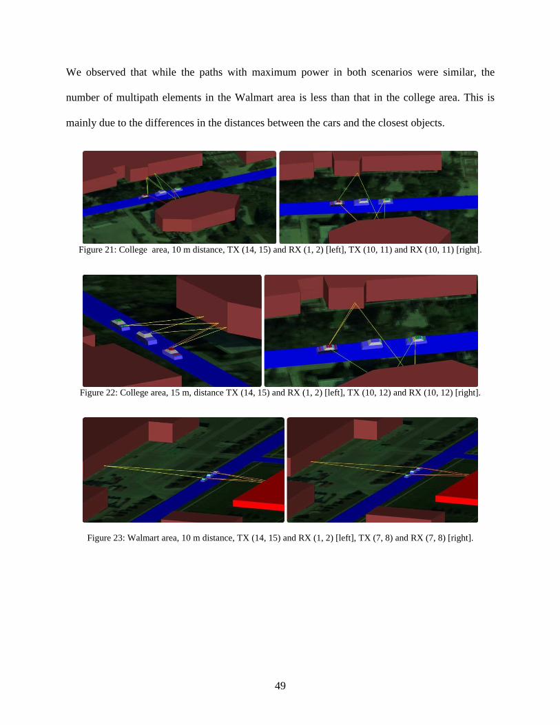
49
We observed that while the paths with maximum power in both scenarios were similar, the
number of multipath elements in the Walmart area is less than that in the college area. This is
mainly due to the differences in the distances between the cars and the closest objects.
Figure 21: College area, 10 m distance, TX (14, 15) and RX (1, 2) [left], TX (10, 11) and RX (10, 11) [right].
Figure 22: College area, 15 m, distance TX (14, 15) and RX (1, 2) [left], TX (10, 12) and RX (10, 12) [right].
Figure 23: Walmart area, 10 m distance, TX (14, 15) and RX (1, 2) [left], TX (7, 8) and RX (7, 8) [right].

50
Figure 24: Walmart area, 15 m distance, TX (1, 2) and RX (1, 2) [left], TX (10, 11) and RX (10, 11) [right].
In this chapter, we consider the same six cases we studied in Chapter 3, while now for all of
them the communication is in NLOS. Figure 21- 24 show the effect of the obstacle vehicle
blocking LOS from TX car to RX car. Three paths with maximum power were selected to see the
number of multipath holding significant value as shown in Figures 21-24.
4.3 Results
4.3.1 Effects of the Antenna Location, Power, and Phase on the Capacity
Tables 14-17 show the relationship between magnitude and phase of the received power with
their respective location on the capacity (including the phase) for all six cases discussed earlier.
Furthermore, it also compares the capacity when the obstacle car exists or is removed, for
distances 10 m and 15 m between the TX car and RX car. Tables 14-17 show these results for
college area-10 m distance, college area-15 m distance, Walmart area-10 m distance and
Walmart area-15 m distance, respectively. The calculated capacities are compared with the
maximum capacity calculated using a 2×2 identity matrix and the average Rayleigh channel
capacity. Similar to Chapter 3, the mean Rayleigh capacity for 2×2 matrix is calculated by taking
average capacity over 1000 iterations of AWGN channels [52]. The capacity for 2×2 identity

51
matrix channel and the 2×2 Rayleigh channel for 20dB SNR are 10.36 and 7.90 bits/s/Hz,
respectively.
Also, it is worth noting the antenna spacing for both scenarios in the first four cases. As
presented in Table 14-17, Cases 2 and 4 yield maximum capacity values in the absence of the
obstacle car, except for Walmart area with 10 m separation where there is nominal difference of
0.64 bits/s/Hz. The spacing between antenna in Cases 2 and 4 are 0.70m (13.20λ) while in Cases
1 and 3 this separation is 0.35m (6.60λ). The increase in capacity due to increase of antenna
separation is expected in conventional MIMO systems [79]. If we compare the roof top cases for
all scenarios, Cases 2 and 4 provide better capacities for 10 m distance and 15 m distance,
respectively, in the absence of obstacle car, whereas, Cases 1 and 3 provide better capacity when
the obstacle is present.
In terms of Case 5, it can be seen in Tables 14 through 17 that college area with 10 m separation
and without obstacle car, and college area with 15 m separation with obstacle car have better
capacities in compare to similar situations in the Walmart area. For other scenarios, capacities in
Walmart area in general are higher than similar scenarios in the college area.

52
Table 14: Channel capacity for six different cases (college area) when the distance between TX and RX is 10 m.
Case TX
RX
Without car (10 m) Capacity
(bits/s/Hz) [With Phase]
With car (10 m) Capacity
(bits/s/Hz) [With Phase]
Power (dBm)
Phase (°)
Power (dBm)
Phase (°)
1
7 7 -65.56 -70.89
8.52
-84.64 -35.69
9.73 7 8 -69.89 -85.23 -69.61 68.55
8 7 -66.41 -140.23 -72.16 162.85
8 8 -66.27 -84.04 -86.84 139.88
2
7 7 -65.56 -70.89
9.06
-84.64 -35.69
8.25 7 9 -67.24 152.00 -82.12 145.42
9 7 -68.29 115.00 -77.31 -104.61
9 9 -67.71 -127.29 -80.01 -65.99
3
10 10 -68.68 -48.68
7.92
-84.25 74.25
9.34 10 11 -67.26 -79.61 -72.62 164.25
11 10 -65.20 -121.46 -73.90 141.08
11 11 -66.53 -91.27 -75.86 -108.37
4
10 10 -68.68 -48.68
8.74
-84.25 74.25
8.97 10 12 -64.77 -133.90 -77.11 -155.88
12 10 -68.53 162.71 -77.32 30.71
12 12 -68.00 -37.22 -78.85 115.43
5
1 14 -104.76 113.94
8.35
-101.55 64.10
6.01 1 15 -81.94 -115.47 -87.38 -108.54
2 14 -86.73 -23.82 -76.27 -31.97
2 15 -95.46 17.18 -82.10 36.41
6
14 1 -64.34 -68.27
6.63
-100.88 -155.15
5.74 14 2 -67.35 60.23 -78.21 -61.11
15 1 -58.45 132.00 -86.22 -176.65
15 2 -65.87 10.10 -75.43 -45.33
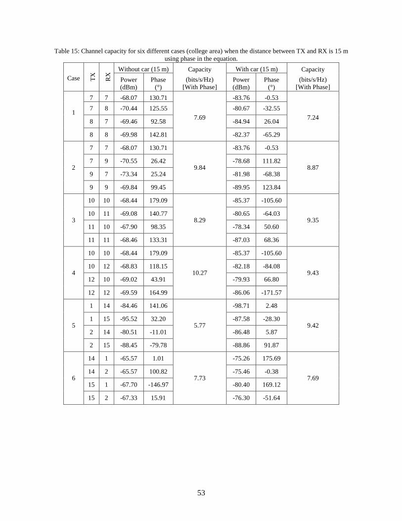
53
Table 15: Channel capacity for six different cases (college area) when the distance between TX and RX is 15 m using phase in the equation.
Case TX
RX
Without car (15 m) Capacity
(bits/s/Hz) [With Phase]
With car (15 m) Capacity
(bits/s/Hz) [With Phase]
Power (dBm)
Phase (°)
Power (dBm)
Phase (°)
1
7 7 -68.07 130.71
7.69
-83.76 -0.53
7.24
7 8 -70.44 125.55 -80.67 -32.55
8 7 -69.46 92.58 -84.94 26.04
8 8 -69.98 142.81 -82.37 -65.29
2
7 7 -68.07 130.71
9.84
-83.76 -0.53
8.87 7 9 -70.55 26.42 -78.68 111.82
9 7 -73.34 25.24 -81.98 -68.38
9 9 -69.84 99.45 -89.95 123.84
3
10 10 -68.44 179.09
8.29
-85.37 -105.60
9.35 10 11 -69.08 140.77 -80.65 -64.03
11 10 -67.90 98.35 -78.34 50.60
11 11 -68.46 133.31 -87.03 68.36
4
10 10 -68.44 179.09
10.27
-85.37 -105.60
9.43 10 12 -68.83 118.15 -82.18 -84.08
12 10 -69.02 43.91 -79.93 66.80
12 12 -69.59 164.99 -86.06 -171.57
5
1 14 -84.46 141.06
5.77
-98.71 2.48
9.42 1 15 -95.52 32.20 -87.58 -28.30
2 14 -80.51 -11.01 -86.48 5.87
2 15 -88.45 -79.78 -88.86 91.87
6
14 1 -65.57 1.01
7.73
-75.26 175.69
7.69 14 2 -65.57 100.82 -75.46 -0.38
15 1 -67.70 -146.97 -80.40 169.12
15 2 -67.33 15.91 -76.30 -51.64
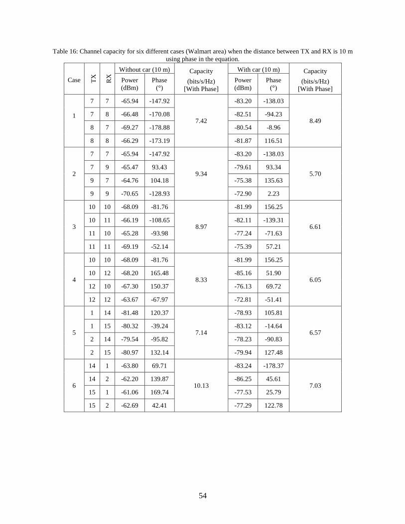
54
Table 16: Channel capacity for six different cases (Walmart area) when the distance between TX and RX is 10 m using phase in the equation.
Case TX
RX
Without car (10 m) Capacity
(bits/s/Hz) [With Phase]
With car (10 m) Capacity
(bits/s/Hz) [With Phase]
Power (dBm)
Phase (°)
Power (dBm)
Phase (°)
1
7 7 -65.94 -147.92
7.42
-83.20 -138.03
8.49 7 8 -66.48 -170.08 -82.51 -94.23
8 7 -69.27 -178.88 -80.54 -8.96
8 8 -66.29 -173.19 -81.87 116.51
2
7 7 -65.94 -147.92
9.34
-83.20 -138.03
5.70 7 9 -65.47 93.43 -79.61 93.34
9 7 -64.76 104.18 -75.38 135.63
9 9 -70.65 -128.93 -72.90 2.23
3
10 10 -68.09 -81.76
8.97
-81.99 156.25
6.61 10 11 -66.19 -108.65 -82.11 -139.31
11 10 -65.28 -93.98 -77.24 -71.63
11 11 -69.19 -52.14 -75.39 57.21
4
10 10 -68.09 -81.76
8.33
-81.99 156.25
6.05 10 12 -68.20 165.48 -85.16 51.90
12 10 -67.30 150.37 -76.13 69.72
12 12 -63.67 -67.97 -72.81 -51.41
5
1 14 -81.48 120.37
7.14
-78.93 105.81
6.57 1 15 -80.32 -39.24 -83.12 -14.64
2 14 -79.54 -95.82 -78.23 -90.83
2 15 -80.97 132.14 -79.94 127.48
6
14 1 -63.80 69.71
10.13
-83.24 -178.37
7.03 14 2 -62.20 139.87 -86.25 45.61
15 1 -61.06 169.74 -77.53 25.79
15 2 -62.69 42.41 -77.29 122.78
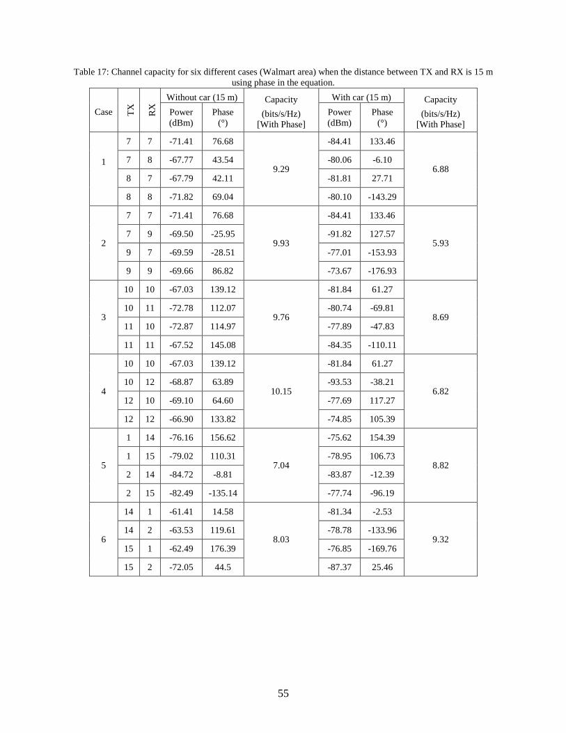
55
Table 17: Channel capacity for six different cases (Walmart area) when the distance between TX and RX is 15 m using phase in the equation.
Case TX
RX
Without car (15 m) Capacity
(bits/s/Hz) [With Phase]
With car (15 m) Capacity
(bits/s/Hz) [With Phase]
Power (dBm)
Phase (°)
Power (dBm)
Phase (°)
1
7 7 -71.41 76.68
9.29
-84.41 133.46
6.88 7 8 -67.77 43.54 -80.06 -6.10
8 7 -67.79 42.11 -81.81 27.71
8 8 -71.82 69.04 -80.10 -143.29
2
7 7 -71.41 76.68
9.93
-84.41 133.46
5.93 7 9 -69.50 -25.95 -91.82 127.57
9 7 -69.59 -28.51 -77.01 -153.93
9 9 -69.66 86.82 -73.67 -176.93
3
10 10 -67.03 139.12
9.76
-81.84 61.27
8.69 10 11 -72.78 112.07 -80.74 -69.81
11 10 -72.87 114.97 -77.89 -47.83
11 11 -67.52 145.08 -84.35 -110.11
4
10 10 -67.03 139.12
10.15
-81.84 61.27
6.82 10 12 -68.87 63.89 -93.53 -38.21
12 10 -69.10 64.60 -77.69 117.27
12 12 -66.90 133.82 -74.85 105.39
5
1 14 -76.16 156.62
7.04
-75.62 154.39
8.82 1 15 -79.02 110.31 -78.95 106.73
2 14 -84.72 -8.81 -83.87 -12.39
2 15 -82.49 -135.14 -77.74 -96.19
6
14 1 -61.41 14.58
8.03
-81.34 -2.53
9.32 14 2 -63.53 119.61 -78.78 -133.96
15 1 -62.49 176.39 -76.85 -169.76
15 2 -72.05 44.5 -87.37 25.46
56
4.3.2 Graphical representations of Capacity vs. SNR
The power and phase received by different antennas at different locations were used to calculate
the channel capacity of the 2×2 MIMO systems. The next two sections present the results of
capacities versus SNR.
4.3.2.1 Capacity Without an Obstacle Car
In this section, the capacities of 2×2 MIMO systems are represented graphically for different
setups (college 10 m, college 15 m, Walmart 10 m, and Walmart 15 m). These capacity values
are further compared with 2×2 identity channel for MIMO capacity (ideal case) and 2×2
Rayleigh MIMO capacities (typical case). In this section the obstacle car between transmitting
and the receiving cars does not exist for distances 10m and 15m for both college and Walmart
scenarios.
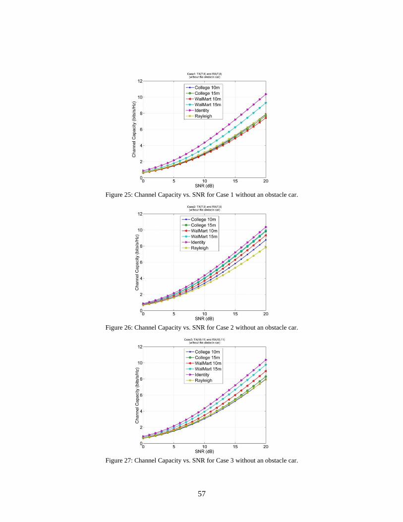
57
Figure 25: Channel Capacity vs. SNR for Case 1 without an obstacle car.
Figure 26: Channel Capacity vs. SNR for Case 2 without an obstacle car.
Figure 27: Channel Capacity vs. SNR for Case 3 without an obstacle car.

58
Figure 28: Channel Capacity vs. SNR for Case 4 without an obstacle car.
Figure 29: Channel Capacity vs. SNR for Case 5 without an obstacle car.
Figure 30: Channel Capacity vs. SNR for Case 6 without an obstacle car.
59
4.3.2.2 Capacity with an Obstacle Car
In this section, the capacities of 2×2 MIMO setups are represented graphically for different
setups (college 10 m, college 15 m, Walmart 10 m, and Walmart 15 m). These capacity values
are further compared with 2×2 Identity MIMO capacity (ideal case) and 2×2 Rayleigh MIMO
capacities (typical case). In this section, an obstacle car is placed between transmitting and the
receiving cars.
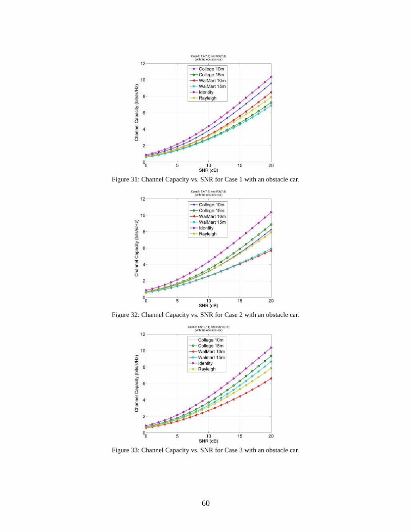
60
Figure 31: Channel Capacity vs. SNR for Case 1 with an obstacle car.
Figure 32: Channel Capacity vs. SNR for Case 2 with an obstacle car.
Figure 33: Channel Capacity vs. SNR for Case 3 with an obstacle car.
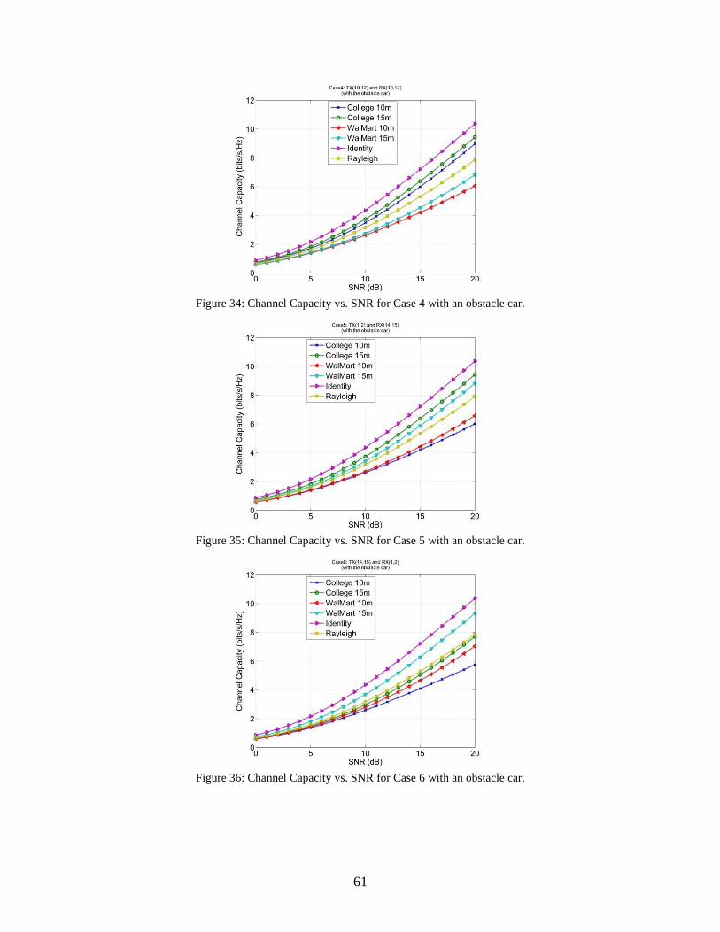
61
Figure 34: Channel Capacity vs. SNR for Case 4 with an obstacle car.
Figure 35: Channel Capacity vs. SNR for Case 5 with an obstacle car.
Figure 36: Channel Capacity vs. SNR for Case 6 with an obstacle car.
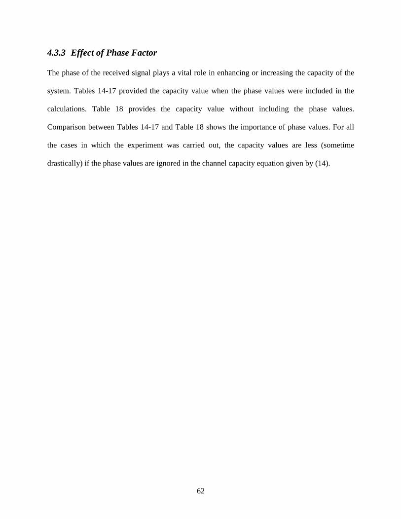
62
4.3.3 Effect of Phase Factor
The phase of the received signal plays a vital role in enhancing or increasing the capacity of the
system. Tables 14-17 provided the capacity value when the phase values were included in the
calculations. Table 18 provides the capacity value without including the phase values.
Comparison between Tables 14-17 and Table 18 shows the importance of phase values. For all
the cases in which the experiment was carried out, the capacity values are less (sometime
drastically) if the phase values are ignored in the channel capacity equation given by (14).

63
Table 18: Channel capacity (bits/s/Hz) for different scenarios and distances when the phase values were excluded.
CA
SE
College 10 m
(without car)
College 10 m
(with car)
College 15 m
(without car)
College 15 m
(with car)
Walmart 10 m
(without car)
Walmart 10 m
(without car)
Walmart 15 m
(without car)
Walmart 15 m
(without car)
1 7.72 9.57 6.24 5.71 7.12 8.49 8.89 6.45
2 7.39 6.91 8.05 8.72 8.12 5.70 6.35 5.93
3 5.73 9.33 5.67 9.34 8.22 6.61 9.59 8.25
4 7.05 8.79 5.67 8.87 6.73 6.05 7.51 6.76
5 9.97 6.00 5.72 9.17 6.71 6.57 6.47 8.73
6 5.80 5.74 5.69 7.21 7.03 7.03 7.30 9.29
4.3.4 K Factor
K-Factor is an important tool to understand the multipath scenario. Higher K-Factor suggests low
scattering path or indirect path. Tables 19 and 20 provide the Mean K (dB) for college and
Walmart areas when the distance between the TX and cars are 10 m and 15 m, respectively.
“Mean (K)” in these tables is the average of K-Factors produced in any selected cases by taking
an average of K-Factors over the four possible channels.
Tables 19 and 20 should be viewed in conjunction with Tables 14-17. Comparing the Cases 1
through 4 from Tables 14-17 and Table 19 and 20, we can see that for scenarios without the
obstacle car in between, cases with low K-Factor has the highest capacity. However from Tables
16 and 19, for Walmart 10 m scenario, where the K-factor is almost the same, ranging from
11.48 to 11.69, Case 2 shows the maximum capacity in which K-Factor equals to 11.65.
Results of the K-Factor and capacities in Cases 5 and 6 are worth paying attention. First, despite
having the same K-Factor value for NLOS condition of Case 5, the capacity of the college area is
higher than that of the Walmart area. In Case 5, transmitters are in the rear of the car with
antenna height of 0.95m, which is clearly obstructed by glass that extends to the roof at the

64
height of 1.35m. Hence, the entire signal are either reflected back or scattered before reaching
the receiver on front of the RX car.
Since the K-Factor of both areas for Case 5 without obstacle car and for all cases with the
obstacle car for both college and Walmart areas are 0 (-∞ in dB), it suggests a rich scattering
environment with NLOS scenario, and the H matrix similar to Rayleigh fading channel [52] is
expected. Their respective capacities are also around the mean Rayleigh capacity. This is true for
most of the cases in Walmart area and some of the cases for the college area. In terms of case 6,
Tables 19 and 20 show that K-Factor for Walmart scenario are less than those for the college
area (higher capacity values).
For the scenarios with the obstacle car, the resulting K-Factor were 0 or (-∞ dB) suggesting that
there were not any direct path travelling from the TX to RX as shown in Figures 21-24.

65
Table 19: K-Factor for 10 m (without car).
Cas
e
Antenna
Positions TX RX
College Area Walmart Area
K-Factor (dB)
Mean
K (dB)
K-Factor
(dB)
Mean
K (dB)
1 TX(7-8) RX(7-8)
7 7 13.64
13.75
11.31
11.48 7 8 13.74 11.34
8 7 13.82 11.33
8 8 13.82 11.92
2 TX(7-9) RX(7-9)
7 7 13.64
13.77
11.31
11.65 7 9 13.70 11.33
9 7 13.86 11.91
9 9 13.91 12.04
3 TX(10-11) RX(10-11)
10 10 13.90
13.92
11.36
11.69 10 11 13.92 11.40
11 10 13.93 11.99
11 11 13.97 12.03
4 TX(10-12) RX(10-12)
10 10 13.90
13.95
11.36
11.66 10 12 13.92 11.38
12 10 13.96 11.88
12 12 14.04 12.02
5 TX(1-2)
RX(14-15)
1 14 -∞
-∞
-∞
-∞ 1 15 -∞ -∞
2 14 -∞ -∞
2 15 -∞ -∞
6 TX(14-15) RX(1-2)
14 1 -0.46
-0.75
0.31
0.11 14 2 -0.51 0.31
15 1 -1.25 -0.06
15 2 -0.76 -0.11
66
Table 20: K-Factor when distance 15 m (without car).
Cas
e
Antenna
Positions TX RX
College Area Walmart Area
K-Factor (dB)
Mean
K (dB)
K-Factor
(dB)
Mean
K (dB)
1 TX(7-8) RX(7-8)
7 7 13.80
14.07
14.80
11.79 7 8 13.91 14.88
8 7 14.66 15.34
8 8 13.91 15.47
2 TX(7-9) RX(7-9)
7 7 13.80
14.02
11.70
11.77 7 9 14.66 11.68
9 7 13.76 11.79
9 9 13.85 11.92
3 TX(10-11) RX(10-11)
10 10 14.26
13.97
11.67
11.76 10 11 13.83 11.70
11 10 14.11 11.84
11 11 13.67 11.87
4 TX(10-12) RX(10-12)
10 10 14.26
13.58
11.67
11.74 10 12 13.79 11.66
12 10 13.09 11.77
12 12 13.17 11.90
5 TX(1-2)
RX(14-15)
1 14 -∞
-∞
- ∞
- ∞ 1 15 -∞ -∞
2 14 -∞ -∞
2 15 -∞ -∞
6 TX(14-15) RX(1-2)
14 1 9.98
9.13
-4.81
-4.83 14 2 10.30 -4.81
15 1 8.64 -4.81
15 2 7.60 -4.94
4.4 Summary
In this chapter, we discussed the relevance of V2V communication and the importance of MIMO
to address NLOS scenarios. The effect of blockage in the form of the obstacle car was studied

67
considering different parameters like antenna location, channel capacity, K-Factor, and phase of
the received signal. We also discussed the best antenna locations for multiple antenna systems by
adopting the MIMO systems. In conclusion, although in general, the MIMO capacity increases
with SNR and antenna spacing, in V2V communication the location of antenna also plays an
important role. MIMO channel capacity does not only depend on the multipath, it may also
depend on the magnitude and phase of the power received and the multipath which depends on
angle of arrival distribution caused by the obstacle.
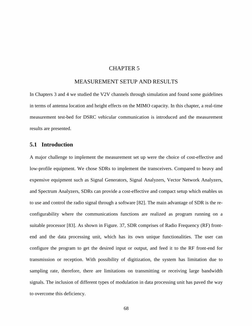
68
CHAPTER 5
MEASUREMENT SETUP AND RESULTS
In Chapters 3 and 4 we studied the V2V channels through simulation and found some guidelines
in terms of antenna location and height effects on the MIMO capacity. In this chapter, a real-time
measurement test-bed for DSRC vehicular communication is introduced and the measurement
results are presented.
5.1 Introduction
A major challenge to implement the measurement set up were the choice of cost-effective and
low-profile equipment. We chose SDRs to implement the transceivers. Compared to heavy and
expensive equipment such as Signal Generators, Signal Analyzers, Vector Network Analyzers,
and Spectrum Analyzers, SDRs can provide a cost-effective and compact setup which enables us
to use and control the radio signal through a software [82]. The main advantage of SDR is the re-
configurability where the communications functions are realized as program running on a
suitable processor [83]. As shown in Figure. 37, SDR comprises of Radio Frequency (RF) front-
end and the data processing unit, which has its own unique functionalities. The user can
configure the program to get the desired input or output, and feed it to the RF front-end for
transmission or reception. With possibility of digitization, the system has limitation due to
sampling rate, therefore, there are limitations on transmitting or receiving large bandwidth
signals. The inclusion of different types of modulation in data processing unit has paved the way
to overcome this deficiency.
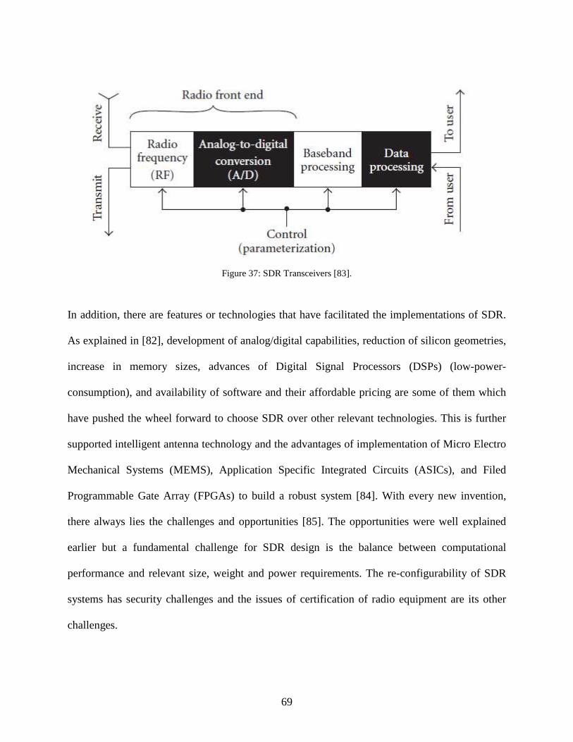
69
Figure 37: SDR Transceivers [83].
In addition, there are features or technologies that have facilitated the implementations of SDR.
As explained in [82], development of analog/digital capabilities, reduction of silicon geometries,
increase in memory sizes, advances of Digital Signal Processors (DSPs) (low-power-
consumption), and availability of software and their affordable pricing are some of them which
have pushed the wheel forward to choose SDR over other relevant technologies. This is further
supported intelligent antenna technology and the advantages of implementation of Micro Electro
Mechanical Systems (MEMS), Application Specific Integrated Circuits (ASICs), and Filed
Programmable Gate Array (FPGAs) to build a robust system [84]. With every new invention,
there always lies the challenges and opportunities [85]. The opportunities were well explained
earlier but a fundamental challenge for SDR design is the balance between computational
performance and relevant size, weight and power requirements. The re-configurability of SDR
systems has security challenges and the issues of certification of radio equipment are its other
challenges.

70
5.2 System Configuration
5.2.1 Hardware
5.2.1.1 Software Defined Radio
Ettus Research™ USRP™ N200 was used as transmitter and receiver units in our experiment, as
shown in Figure. 38. The detailed architecture of the USRP™ N200 is shown in Figure. 39.
Figure 38: Ettus Research™ USRP™ N200 used as SDR.
USRP™ N200 is one of the highest performing class of hardware of the USRPTM family of
products, which enables user to rapidly design and implement powerful, flexible software radio
systems. It offers MIMO capability with high bandwidth and dynamic range. The Gigabit
Ethernet interface serves as the connection between the N200 and the host computer. This
enables the user to realize 50MS/s of real-time bandwidth in the receiver and transmit directions,
simultaneously (full duplex).
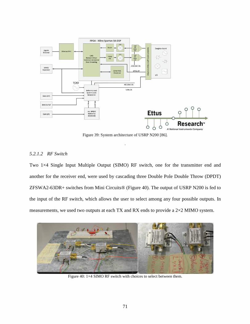
71
Figure 39: System architecture of USRP N200 [86].
.
5.2.1.2 RF Switch
Two 1×4 Single Input Multiple Output (SIMO) RF switch, one for the transmitter end and
another for the receiver end, were used by cascading three Double Pole Double Throw (DPDT)
ZFSWA2-63DR+ switches from Mini Circuits® (Figure 40). The output of USRP N200 is fed to
the input of the RF switch, which allows the user to select among any four possible outputs. In
measurements, we used two outputs at each TX and RX ends to provide a 2×2 MIMO system.
Figure 40: 1×4 SIMO RF switch with choices to select between them.

72
5.2.1.3 High Gain Amplifier
In an experiment with spectrum analyzer and USRP N200 at 2.4 GHz the output of USRP is -4
dBm (4mW) was noticed at 0dBm reference of spectrum analyzer, when USRP was directly
connected to the spectrum analyzer through an SMA cable. This level was 6 dBm for -10dBm
reference shown by spectrum analyzer. The output of the spectrum analyzer was decreased to -15
dBm from 6 dBm when an antenna was used at a distance of 0.5 m between spectrum analyzer
and USRP. This clearly shows the power loss and the pathloss phenomena. As our motive was to
use USRP in outdoor settings, at a maximum distance of 15 m, the signal would practically be at
the noise level. To overcome two high gain amplifiers (ZVE-8G+), from Mini Circuits® with 30
dB gain at 5.9 GHz (our intended working frequency), as shown in Figure 41, were used.
Figure 41: High gain amplifiers used at the transmitter end.
5.2.1.4 Antenna
We used VERT2450 antenna, an Ettus Research™ product (Figure 42) which is a dual band
antennas working within the bands of 2.4 GHz to 2.48 GHz, and 4.9 GHz to 5.9 GHz. This is an
Omni-directional vertical antenna. The antenna was used at 5.9 GHz (wavelength of 0.053m).

73
Figure 42: VERT2450 Antenna (Ettus Research™).
5.2.1.5 Cables, Adapters and Terminators
When a high gain amplifier is added to the setup, it is very important to select appropriate
components for safe operation. The cables must be made for the range of working frequency to
avoid mismatching. The matched terminators must be used to avoid creation of open circuits at
the end of the system that cause high reflections to the digital unit (USRP, in our case) resulting
in damage. Care must be taken when adaptors are used for connecting cables. Co-axial cable
with male SMA connection was used in this measurement. Female to female SMA adapter were
used to connect male antenna to male SMA cable. 50 ohm terminators were used to terminate the
switch port (not being used) at both transmitting and receiving end.
Figure 43: Terminators and antennas.
5.2.2 Software
There are various available software options to drive the hardware. GNU Radio, for Linux
platform, National Instruments (NI) LabVIEW and Matlab Simulink for windows platform are

74
some popular tools. In this work, we have used LabVIEW basically for two reasons. First, the
Graphical User Interface (GUI) and configurability of LabVIEW makes it simple and easy to
program the SDR. Second, since there is collaboration between NI and Ettus research, the
technical support and help in debugging and troubleshooting the problems speed up the process
of implementation of the design. Matlab from MathWorks is used for processing the data
received from LabVIEW to get the desired output.
5.2.2.1 National Instrument’s LabVIEW
LabVIEW is a graphical programming platform that allows the user to design and test the
systems. In this thesis, we present LabVIEW as an interface between USRP N200 (radio) and the
program that controls the radio. This allows using desired modulation techniques for
transmission and demodulation techniques for receiving. We used IQ modulation and
demodulation as shown in the Figures 44 and 45. A 1 KHz message signal is modulated at 5.9
GHz (DSRC band) at the transmitter and the power and phase are monitored at the receiver end.
The detail operation is described in Section 5.3.2.
5.2.2.2 Matlab
The received values for power and phase are further processed in Matlab to calculate the
capacity (bits/s/Hz) for different antenna locations in TX and RX ends.

75
Figure 44: Transmitter end LabVIEW window.
Figure 45: Receiver end LabVIEW window.
5.3 Methodology
The location and setup of measurement were decided based on the experiment requirements and
following the simulation setups. Our primary objective was to replicate the exact location and
distances of antenna and cars used in the simulation done in Wireless InSite®.

76
5.3.1 System Set Up
Following the same setup for simulation, in each measurement we considered 15 TX and 15 RX
locations. In each measurement we considered one of the six cases of interest of 2×2 MIMO. So
at each measurement we placed two TX antennas and two RX antennas. The active antennas
were controlled by switch. The distance between the antennas was measured to be similar to
simulation setup. The location of antenna was similar to that of simulation as shown in Figure
46.
Figure 46: Location of antenna for measurement.
5.3.1.1 Device Platform
There were multiple electronic devices used in the measurement. These devices were running on
the car battery. To minimize the time of measurements a wooden platform was designed to keep
each component in a static location, this minimizes the errors due to phase changes of cables and
prevents the problem of loose connections. Figure 47 shows the platform built for both TX and
RX ends. TX ends consists of two high gain amplifiers, 1×4 RF switch, USRP N200, and
extension cord. The RX end consist only of USRP, 1×4 RF switch and extension cord.
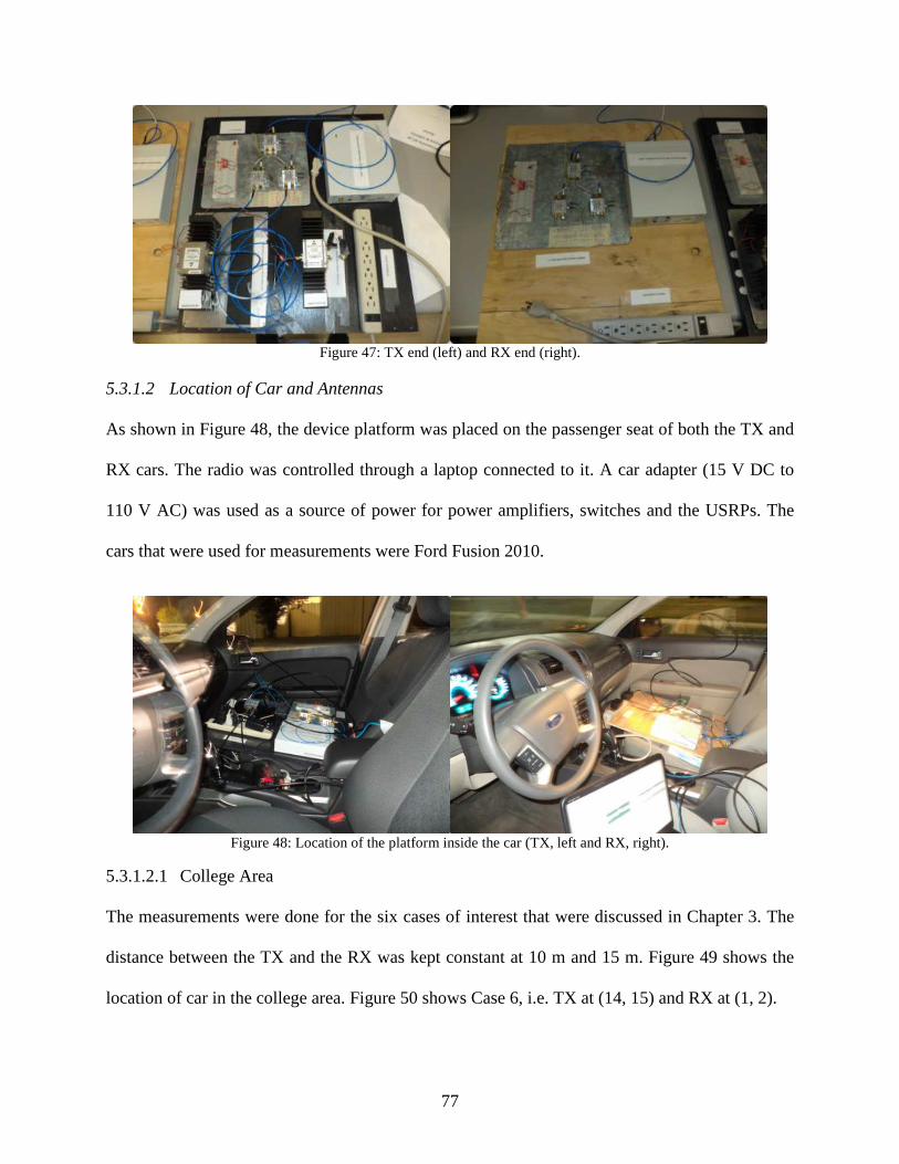
77
Figure 47: TX end (left) and RX end (right).
5.3.1.2 Location of Car and Antennas
As shown in Figure 48, the device platform was placed on the passenger seat of both the TX and
RX cars. The radio was controlled through a laptop connected to it. A car adapter (15 V DC to
110 V AC) was used as a source of power for power amplifiers, switches and the USRPs. The
cars that were used for measurements were Ford Fusion 2010.
Figure 48: Location of the platform inside the car (TX, left and RX, right).
5.3.1.2.1 College Area
The measurements were done for the six cases of interest that were discussed in Chapter 3. The
distance between the TX and the RX was kept constant at 10 m and 15 m. Figure 49 shows the
location of car in the college area. Figure 50 shows Case 6, i.e. TX at (14, 15) and RX at (1, 2).

78
Figure 49: TX and Rx cars in the college area at 10 m distance.
Figure 50: Antennas placement on TX (left) and on RX (right).
5.3.1.2.2 Walmart Area
Similar to college area, the measurement in Walmart area was done for six cases keeping the
distance between the TX and the RX, first at 10 m and 15 m. Figure 51 shows the cars in the
Walmart area. Figure 52 shows Case 2, i.e. TX at (10, 12) and RX at (10, 12).
Figure 51: Transmitter car and receiver car with distance 10 m in Walmart area.
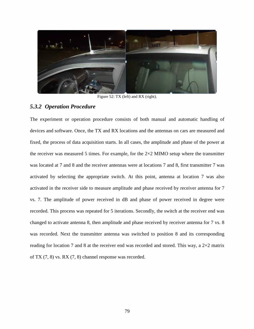
79
Figure 52: TX (left) and RX (right).
5.3.2 Operation Procedure
The experiment or operation procedure consists of both manual and automatic handling of
devices and software. Once, the TX and RX locations and the antennas on cars are measured and
fixed, the process of data acquisition starts. In all cases, the amplitude and phase of the power at
the receiver was measured 5 times. For example, for the 2×2 MIMO setup where the transmitter
was located at 7 and 8 and the receiver antennas were at locations 7 and 8, first transmitter 7 was
activated by selecting the appropriate switch. At this point, antenna at location 7 was also
activated in the receiver side to measure amplitude and phase received by receiver antenna for 7
vs. 7. The amplitude of power received in dB and phase of power received in degree were
recorded. This process was repeated for 5 iterations. Secondly, the switch at the receiver end was
changed to activate antenna 8, then amplitude and phase received by receiver antenna for 7 vs. 8
was recorded. Next the transmitter antenna was switched to position 8 and its corresponding
reading for location 7 and 8 at the receiver end was recorded and stored. This way, a 2×2 matrix
of TX (7, 8) vs. RX (7, 8) channel response was recorded.
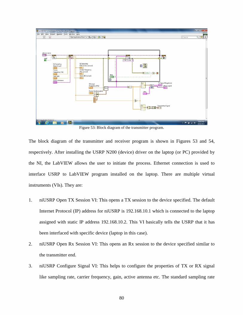
80
Figure 53: Block diagram of the transmitter program.
The block diagram of the transmitter and receiver program is shown in Figures 53 and 54,
respectively. After installing the USRP N200 (device) driver on the laptop (or PC) provided by
the NI, the LabVIEW allows the user to initiate the process. Ethernet connection is used to
interface USRP to LabVIEW program installed on the laptop. There are multiple virtual
instruments (VIs). They are:
1. niUSRP Open TX Session VI: This opens a TX session to the device specified. The default
Internet Protocol (IP) address for niUSRP is 192.168.10.1 which is connected to the laptop
assigned with static IP address 192.168.10.2. This VI basically tells the USRP that it has
been interfaced with specific device (laptop in this case).
2. niUSRP Open Rx Session VI: This opens an Rx session to the device specified similar to
the transmitter end.
3. niUSRP Configure Signal VI: This helps to configure the properties of TX or RX signal
like sampling rate, carrier frequency, gain, active antenna etc. The standard sampling rate
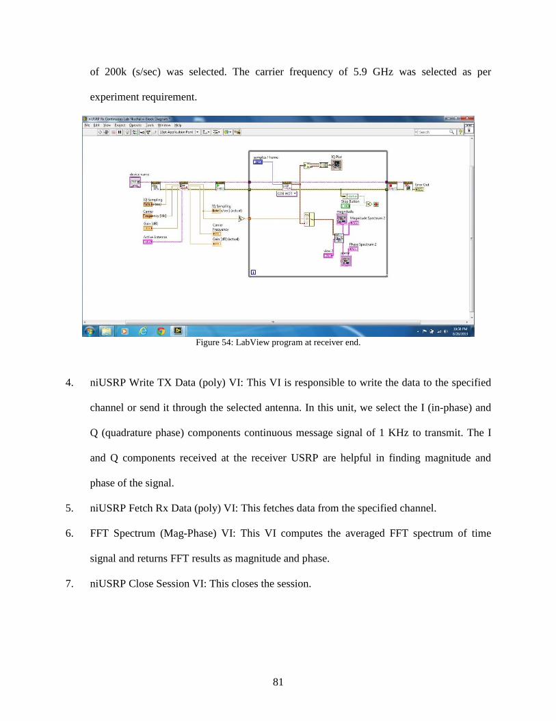
81
of 200k (s/sec) was selected. The carrier frequency of 5.9 GHz was selected as per
experiment requirement.
Figure 54: LabView program at receiver end.
4. niUSRP Write TX Data (poly) VI: This VI is responsible to write the data to the specified
channel or send it through the selected antenna. In this unit, we select the I (in-phase) and
Q (quadrature phase) components continuous message signal of 1 KHz to transmit. The I
and Q components received at the receiver USRP are helpful in finding magnitude and
phase of the signal.
5. niUSRP Fetch Rx Data (poly) VI: This fetches data from the specified channel.
6. FFT Spectrum (Mag-Phase) VI: This VI computes the averaged FFT spectrum of time
signal and returns FFT results as magnitude and phase.
7. niUSRP Close Session VI: This closes the session.
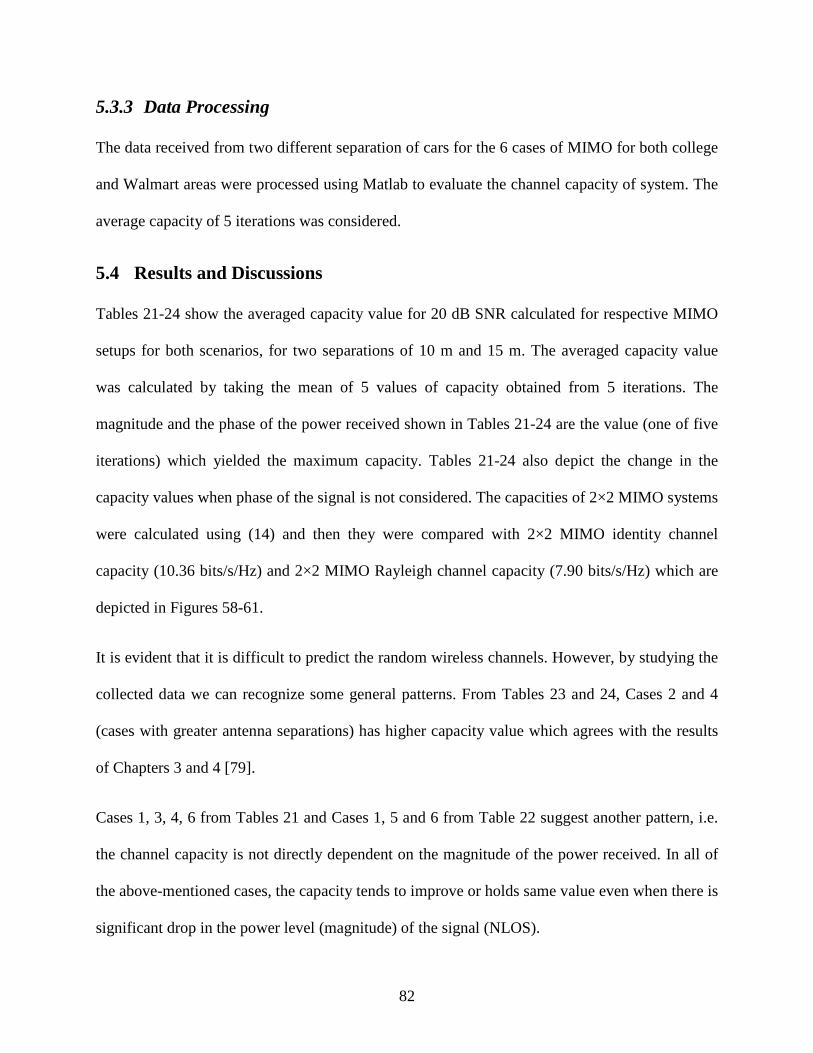
82
5.3.3 Data Processing
The data received from two different separation of cars for the 6 cases of MIMO for both college
and Walmart areas were processed using Matlab to evaluate the channel capacity of system. The
average capacity of 5 iterations was considered.
5.4 Results and Discussions
Tables 21-24 show the averaged capacity value for 20 dB SNR calculated for respective MIMO
setups for both scenarios, for two separations of 10 m and 15 m. The averaged capacity value
was calculated by taking the mean of 5 values of capacity obtained from 5 iterations. The
magnitude and the phase of the power received shown in Tables 21-24 are the value (one of five
iterations) which yielded the maximum capacity. Tables 21-24 also depict the change in the
capacity values when phase of the signal is not considered. The capacities of 2×2 MIMO systems
were calculated using (14) and then they were compared with 2×2 MIMO identity channel
capacity (10.36 bits/s/Hz) and 2×2 MIMO Rayleigh channel capacity (7.90 bits/s/Hz) which are
depicted in Figures 58-61.
It is evident that it is difficult to predict the random wireless channels. However, by studying the
collected data we can recognize some general patterns. From Tables 23 and 24, Cases 2 and 4
(cases with greater antenna separations) has higher capacity value which agrees with the results
of Chapters 3 and 4 [79].
Cases 1, 3, 4, 6 from Tables 21 and Cases 1, 5 and 6 from Table 22 suggest another pattern, i.e.
the channel capacity is not directly dependent on the magnitude of the power received. In all of
the above-mentioned cases, the capacity tends to improve or holds same value even when there is
significant drop in the power level (magnitude) of the signal (NLOS).
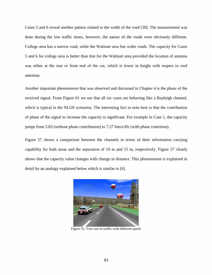
83
Cases 5 and 6 reveal another pattern related to the width of the road [39]. The measurement was
done during the low traffic times, however, the nature of the roads were obviously different.
College area has a narrow road, while the Walmart area has wider roads. The capacity for Cases
5 and 6 for college area is better than that for the Walmart area provided the location of antenna
was either at the rear or front end of the car, which is lower in height with respect to roof
antennas.
Another important phenomenon that was observed and discussed in Chapter 4 is the phase of the
received signal. From Figure 61 we see that all six cases are behaving like a Rayleigh channel,
which is typical in the NLOS scenarios. The interesting fact to note here is that the contribution
of phase of the signal to increase the capacity is significant. For example in Case 1, the capacity
jumps from 5.83 (without phase contribution) to 7.27 bits/s/Hz (with phase contrition).
Figure 57 shows a comparison between the channels in terms of their information carrying
capability for both areas and the separation of 10 m and 15 m, respectively. Figure 57 clearly
shows that the capacity value changes with change in distance. This phenomenon is explained in
detail by an analogy explained below which is similar to [6].
Figure 55: Two cars in traffic with different speed.
84
Figure 56: Spectrum decision management loop based on channel capacity[6].
Suppose two cars (Figure 55) are travelling at a constant velocity 20 miles/hr in the traffic at the
residential area (with same speed limit), maintaining the distance between the cars to be 5 m.
Now, the driver of the vehicle travelling behind wants to overtake the vehicle in front of him. He
does this by increasing the velocity of his car to 25 miles/hr (40 Km/hr). In that case, time taken
by that vehicle to travel 5 m distance will be 450 milliseconds (ms). The car will travel the same
distance with 75 miles/hr. in 140ms. This means, the faster the car quicker the system to respond.
This leads us to an interesting way to view the averaged capacity graphs depicted in Figure 57 to
develop a smart unit, which shows the highest capacity value for each Case for both scenarios.
The best connection between two cars can be established based on the capacity they share with
each other. From Table 22, out of six cases, Case 6 provides the best capacity results for college
area i.e. 9.27 bits/s/Hz. In travelling the 5m distance, still Case 6 provides the best capacity i.e.
9.28 bits/s/Hz (from Table 21) in compare to of all other antenna locations. Hence the smart unit
can make a decision to connect the travelling car (overtaking car) whose antenna location yields
the best capacity when incorporated with the overtaken car.
85
Similarly, from Table 24, for Walmart area, Case 6 is the best combination of antennas setup that
yields the largest capacity (7.85 bits/s/Hz) but the system needs to switch the antenna
combination to Case 2 with capacity 8.79 bits/s/Hz (Table 23) when it travels and has the 5m as
the differential distance.
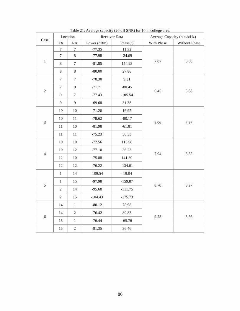
86
Table 21: Average capacity (20 dB SNR) for 10 m college area.
Case Location Receiver Data Average Capacity (bits/s/Hz)
TX RX Power (dBm) Phase(º) With Phase Without Phase
1
7 7 -77.35 11.32
7.87 6.08
7 8 -77.98 -24.69
8 7 -81.85 154.93
8 8 -80.00 27.86
2
7 7 -78.38 9.31
6.45 5.88 7 9 -71.71 -80.45
9 7 -77.43 -105.54
9 9 -69.68 31.38
3
10 10 -71.20 16.95
8.06 7.97 10 11 -78.62 -80.17
11 10 -81.98 -61.81
11 11 -75.23 56.33
4
10 10 -72.56 113.98
7.94 6.85 10 12 -77.10 36.23
12 10 -75.88 141.39
12 12 -76.22 -134.01
5
1 14 -109.54 -19.04
8.70 8.27 1 15 -97.98 -159.87
2 14 -95.68 -111.75
2 15 -104.43 -175.73
6
14 1 -80.12 78.98
9.28 8.66 14 2 -76.42 89.83
15 1 -76.44 -65.76
15 2 -81.35 36.46

87
Table 22: Average capacity (20 dB SNR) for 15 m college area.
Case Location Receiver Data Capacity (bits/s/Hz)
TX RX Power (dBm) Phase(º) With Phase Without Phase
1
7 7 -93.59 65.18
8.17 6.67
7 8 -87.17 -129.39
8 7 -91.31 105.14
8 8 -91.82 91.03
2
7 7 -93.58 20.75
6.18 5.84 7 9 -85.88 70.69
9 7 -95.93 -124.37
9 9 -88.86 81.03
3
10 10 -90.59 40.05
9.23 6.77 10 11 -89.43 63.20
11 10 -89.26 -62.07
11 11 -89.80 100.99
4
10 10 -98.90 -121.40
8.90 8.28 10 12 -87.30 150.44
12 10 -89.56 129.09
12 12 -91.78 148.81
5
1 14 -105.43 -25.99
8.67 8.34 1 15 -96.04 92.62
2 14 -95.52 -77.71
2 15 -109.14 100.11
6
14 1 -96.52 32.74
9.27 8.79 14 2 -91.67 -6.98
15 1 -92.35 14.44
15 2 -103.96 125.24

88
Table 23: Averaged capacity (20 dB SNR) for 10 m Walmart area.
Case Location Receiver Data Capacity (bits/s/Hz)
TX RX Power (dBm) Phase(º) With Phase Without Phase
1
7 7 -73.58 87.46
6.03 5.68 7 8 -77.24 139.78
8 7 -81.98 -59.19
8 8 -83.98 144.37
2
7 7 -75.29 119.39
8.79 8.13 7 9 -80.70 117.17
9 7 -75.80 -90.13
9 9 -73.95 105.30
3
10 10 -78.19 171.21
8.03 6.99 10 11 -77.33 -3.58
11 10 -80.08 -73.76
11 11 -82.57 -88.53
4
10 10 -78.84 -108.86
8.06 7.12 10 12 -79.54 156.39
12 10 -78.91 -10.10
12 12 -76.27 164.83
5
1 14 -92.93 151.12
5.81 5.72 1 15 -99.71 78.18
2 14 -88.30 -97.02
2 15 -96.69 100.44
6
14 1 -92.02 108.46
8.65 8.60 14 2 -81.81 -139.48
15 1 -81.16 -131.84
15 2 -85.34 80.48
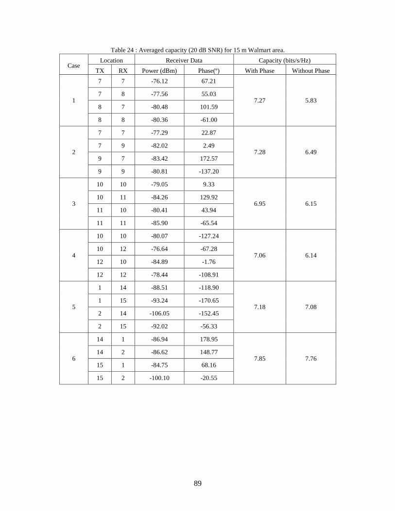
89
Table 24 : Averaged capacity (20 dB SNR) for 15 m Walmart area.
Case Location Receiver Data Capacity (bits/s/Hz)
TX RX Power (dBm) Phase(º) With Phase Without Phase
1
7 7 -76.12 67.21
7.27 5.83 7 8 -77.56 55.03
8 7 -80.48 101.59
8 8 -80.36 -61.00
2
7 7 -77.29 22.87
7.28 6.49 7 9 -82.02 2.49
9 7 -83.42 172.57
9 9 -80.81 -137.20
3
10 10 -79.05 9.33
6.95 6.15 10 11 -84.26 129.92
11 10 -80.41 43.94
11 11 -85.90 -65.54
4
10 10 -80.07 -127.24
7.06 6.14 10 12 -76.64 -67.28
12 10 -84.89 -1.76
12 12 -78.44 -108.91
5
1 14 -88.51 -118.90
7.18 7.08 1 15 -93.24 -170.65
2 14 -106.05 -152.45
2 15 -92.02 -56.33
6
14 1 -86.94 178.95
7.85 7.76 14 2 -86.62 148.77
15 1 -84.75 68.16
15 2 -100.10 -20.55
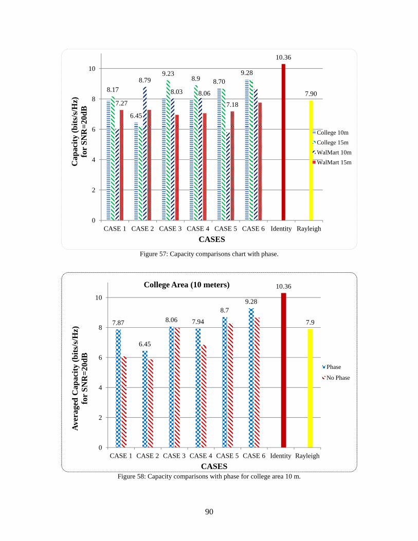
90
Figure 57: Capacity comparisons chart with phase.
Figure 58: Capacity comparisons with phase for college area 10 m.
6.45
8.709.28
8.17
9.238.98.79
8.03 8.06
10.36
7.90
7.27 7.18
0
2
4
6
8
10
CASE 1 CASE 2 CASE 3 CASE 4 CASE 5 CASE 6 Identity Rayleigh
Cap
acity
(bi
ts/s
/Hz)
for
SN
R=
20dB
CASES
College 10m
College 15m
WalMart 10m
WalMart 15m
7.87
6.45
8.06 7.94
8.79.28
10.36
7.9
0
2
4
6
8
10
CASE 1 CASE 2 CASE 3 CASE 4 CASE 5 CASE 6 Identity Rayleigh
Ave
rage
d C
apac
ity (
bits
/s/H
z)fo
r S
NR
=20
dB
CASES
College Area (10 meters)
Phase
No Phase
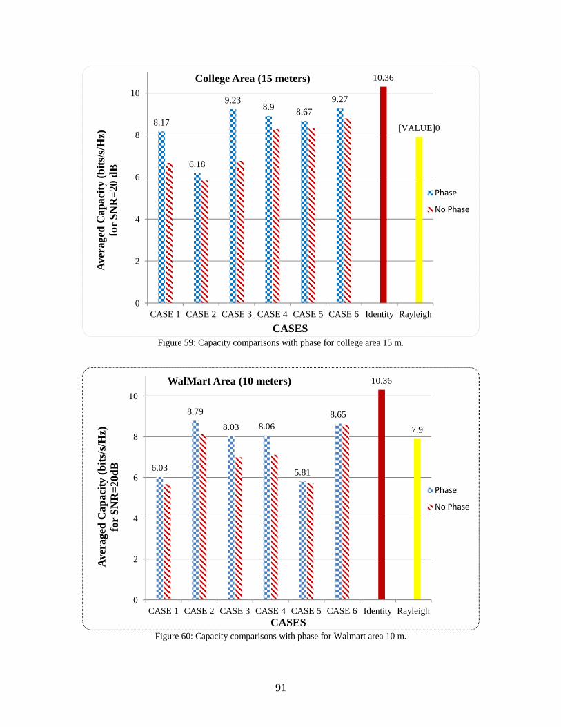
91
Figure 59: Capacity comparisons with phase for college area 15 m.
Figure 60: Capacity comparisons with phase for Walmart area 10 m.
8.17
6.18
9.238.9 8.67
9.27
10.36
[VALUE]0
0
2
4
6
8
10
CASE 1 CASE 2 CASE 3 CASE 4 CASE 5 CASE 6 Identity Rayleigh
Ave
rage
d C
apac
ity (
bits
/s/H
z)fo
r S
NR
=20
dB
CASES
College Area (15 meters)
Phase
No Phase
6.03
8.79
8.03 8.06
5.81
8.65
10.36
7.9
0
2
4
6
8
10
CASE 1 CASE 2 CASE 3 CASE 4 CASE 5 CASE 6 Identity Rayleigh
Ave
rage
d C
apac
ity (
bits
/s/H
z)fo
r S
NR
=20
dB
CASES
WalMart Area (10 meters)
Phase
No Phase
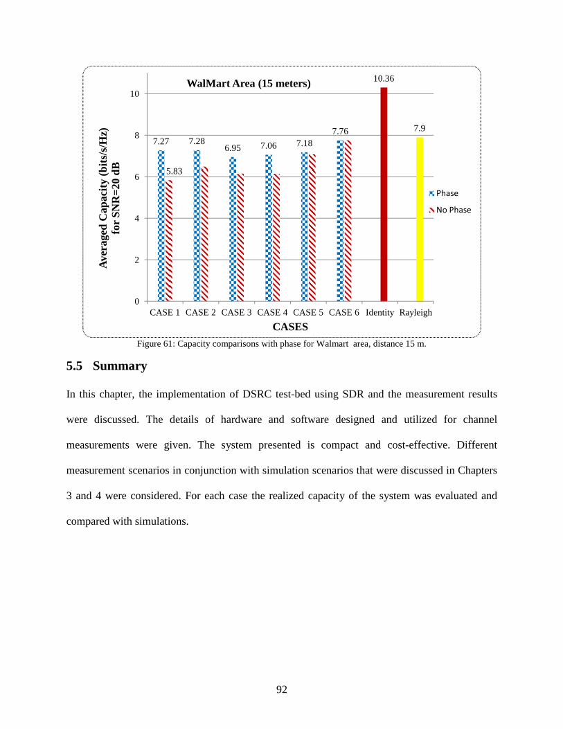
92
Figure 61: Capacity comparisons with phase for Walmart area, distance 15 m.
5.5 Summary
In this chapter, the implementation of DSRC test-bed using SDR and the measurement results
were discussed. The details of hardware and software designed and utilized for channel
measurements were given. The system presented is compact and cost-effective. Different
measurement scenarios in conjunction with simulation scenarios that were discussed in Chapters
3 and 4 were considered. For each case the realized capacity of the system was evaluated and
compared with simulations.
7.27 7.286.95 7.06 7.18
7.76
5.83
10.36
7.9
0
2
4
6
8
10
CASE 1 CASE 2 CASE 3 CASE 4 CASE 5 CASE 6 Identity Rayleigh
Ave
rage
d C
apac
ity (
bits
/s/H
z)fo
r S
NR
=20
dB
CASES
WalMart Area (15 meters)
Phase
No Phase
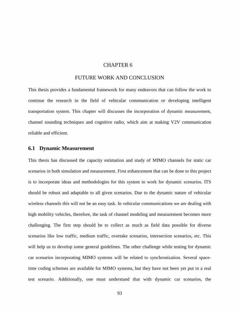
93
CHAPTER 6
FUTURE WORK AND CONCLUSION
This thesis provides a fundamental framework for many endeavors that can follow the work to
continue the research in the field of vehicular communication or developing intelligent
transportation system. This chapter will discusses the incorporation of dynamic measurement,
channel sounding techniques and cognitive radio, which aim at making V2V communication
reliable and efficient.
6.1 Dynamic Measurement
This thesis has discussed the capacity estimation and study of MIMO channels for static car
scenarios in both simulation and measurement. First enhancement that can be done to this project
is to incorporate ideas and methodologies for this system to work for dynamic scenarios. ITS
should be robust and adaptable to all given scenarios. Due to the dynamic nature of vehicular
wireless channels this will not be an easy task. In vehicular communications we are dealing with
high mobility vehicles, therefore, the task of channel modeling and measurement becomes more
challenging. The first step should be to collect as much as field data possible for diverse
scenarios like low traffic, medium traffic, overtake scenarios, intersection scenarios, etc. This
will help us to develop some general guidelines. The other challenge while testing for dynamic
car scenarios incorporating MIMO systems will be related to synchronization. Several space-
time coding schemes are available for MIMO systems, but they have not been yet put in a real
test scenario. Additionally, one must understand that with dynamic car scenarios, the
94
vehicular propagation channel may be very different than cellular channels, yielding new
parameters that affect delay and Doppler spreads.
6.2 Channel Sounding Techniques
The importance of channel capacity as a crucial parameter to study the channel and its ability to
carry information was discussed in this thesis. Other parameters such as pathloss, angle of
arrival, delay spread, Doppler might be carefully studied as a function of vehicle’s speed,
environment and vehicle’s size. Channel sounding techniques are ways to collect and measure
CIR and study the effects of different parameters on the signal strength travelling from
transmitter to the receiver. The measurement setup that is presented in this thesis may be used in
future for studying these parameters, the only modification that needs to be done is in the
software.
6.3 Cognitive Radio
Adding an artificial intelligence to the existing setup that was presented in this thesis can yield an
adaptive wireless sensor network, often defined as cognitive radio. Cognitive radio is hailed as
the ultimate evolution of SDRs which will be able to access the vehicular propagation
parameters, spectrum usage and adapt to the RF environment accordingly. To achieve this, such
smart unit should be trained with tons of information about the channel in different scenarios.
Future works described earlier are the initial steps to be accomplished before dwelling on
implementation of the cognitive radio concepts.
6.4 Conclusion
This thesis has presented a system level idea and design of a robust tool to investigate the MIMO
channels utilization in DSRC. We proposed the use of SDR for channel sounding and ray-tracing
95
for channel simulation. The channel capacity was used as a measure to examine the MIMO
channels in terms of antenna selection for best utilization of multipath. In the channel simulation
some channel parameters like K-Factor, and capacity were analyzed with respect to antenna
location. The similar setup was used to measure the channel capacity in real scenario using
SDRs. The results of these measurement campaign and simulations gave us insight of how the
vehicular propagation channel behaves. The relation of antenna location to channel capacity, K-
Factor relation to multipath, importance of phase of the received angle in defining the diversity
of the system was studied. The purposed setup for measurement can further be enhanced to
achieve the goals discussed as future work.

APPENDICES

97
APPENDIX A
CHANNEL CAPACITY CALCULATION (MATLAB)
clear all ; clc; %%%%%%%%%%%%%%%%%%%%%%%%%%%%%%%%%%%%%%%%%%% %%% IMPORTING FILES %%%% %%%%%%%%%%%%%%%%%%%%%%%%%%%%%%%%%%%%%%%%%%% file= 'WALWCar15.xlsx' ; sheet=1; data= 'C5:AF19' ; A=xlsread(file,sheet,data); snrdb=[0: 1: 20]; %snrdb=[0: 1: 20]; snr=10.^(snrdb/10); %color = ['b';'r';'g';'k';'c']; %notation = ['-o';'->';'<-';'-^';'-s']; nT=2; nR=2; K=2; %Ricean K-factor2 for i=1 : nT*nR; T(i)= input( 'Select Tx :' ); %User INPUT for desired transmitter R(i)=input( 'Select Rx:' ); %User INPUT for desired receiver M(i)=A(T(i), (R(i)-1)*2+1) %accessing Magnitude in dbm for given TX and RX Mag(i)=10.^(M(i)/10)*10^-3 ; %changing dbm into watts P(i)=A(T(i),R(i)*2) %accessing Phase in deg for given TX and RX Phase(i)=P(i)*(pi/180); %changing deg. into
98
radians H(i)=Mag(i)*exp(j*(Phase(i))); %Expressing in form of : |Hij|.exp(jANGij)Ref: Page 2: On the capacity of th e MIMO channel -Bengt Hotler end Mag1= Mag(1)+Mag(3); %Mag1mw=Mag1/0.001; %Mag1dBm=20*log(Mag1mw); Mag2=Mag(2)+Mag(4); %Mag2mw=Mag2/0.001; %Mag2dBm=20*log(Mag2mw); H_d=ones(nT,nR); H_par = [ H(1) H(2) ; H(3) H(4) ]; H_idn = [1 0 ;0 1]; %Identity Matrix H_ray=(randn(nT,nR)+j*randn(nT,nR))/sqrt(2); %Rayleigh Matrix H_ric= sqrt(K/(K+1))*H_d +sqrt(1/(K+1))*H_ray; %Rician Matrix %%%%%%%%%%%%%%%%%%%%%%%%%%%%%%%%%%%%%%%%%%%%%%%%%%%%%% %%%%%%%%%% Capacity for Simulation Matrix %%%%%%%%%%%% %%%%%%%%%%%%%%%%%%%%%%%%%%%%%%%%%%%%%%%%%%%%%%%%%%%%%% CT_H_par = H_par'; %CT_H_par1 = ctranspose(H_par) H_product= H_par*CT_H_par ; H_normalised= H_product/norm(H_product, 'fro' ); lamda= svd(H_normalised); for i=1:length(snr) %T=snrdb(i); %Y=log2(snrdb(i).*(lamda.^2)); %C(i)= sum(1 + log2(snr(i).*(lamda.^2))); %C(i)=log2(real(det(I + (snr(i)./nT).* HProd))) C(i)=0; for j=1:length(lamda) C(i)=C(i)+log2(1+snr(i)/nT*lamda(j)); end end CapacityMAX_Simulation_10dB=C(11) CapacityMAX_Simulation_20dB=C(21) hold all grid on plot(snrdb,C, '--' ) xlabel( 'SNR dB' ) ylabel( 'Channel Capacity(bits/s/hz) ' ) %%%%%%%%%%%%%%%%%%%%%%%%%%%%%%%%%%%%%%%%%%%%%%%%%%%%%% %%%%%%%%%%% Capacity for Identity Matrix %%%%%%%%%%%%% %%%%%%%%%%%%%%%%%%%%%%%%%%%%%%%%%%%%%%%%%%%%%%%%%%%%%% CT_H_idn = H_idn'; %CT_H_par1 = ctranspose(H_par)
99
H_product_idn= H_idn*CT_H_idn ; H_normalised_idn= H_product_idn/norm(H_product_idn , 'fro' ); lamda_idn= svd(H_normalised_idn); for i=1:length(snr) C(i)=0; for j=1:length(lamda_idn) C(i)=C(i)+log2(1+snr(i)/nT*lamda_idn(j)); end end %CapacityMAX_Identity_10dB=C(11) CapacityMAX_Identity_20dB=C(21) hold all grid on plot(snrdb,C, '--' ) %xlabel('SNR (dB)') %ylabel('Channel Capacity (bits/s/hz) ') %%%%%%%%%%%%%%%%%%%%%%%%%%%%%%%%%%%%%%%%%%%%%%%%%%%%%% %%%%%%%%%%% Capacity for Rayleigh Matrix %%%%%%%%%%%%% %%%%%%%%%%%%%%%%%%%%%%%%%%%%%%%%%%%%%%%%%%%%%%%%%%%%%% for m=1:1:1000 H_ray=(randn(2,2)+j*randn(2,2))/sqrt(2); CT_H_ray = H_ray'; H_product_ray= H_ray*CT_H_ray ; H_normalised_ray= H_product_ray/norm(H_product_ray , 'fro' ); lamda_ray= svd(H_normalised_ray); for i=1:length(snr) C(i)=0; for j=1:length(lamda_ray) C(i)=C(i)+log2(1+snr(i)/2*lamda_ray(j)); end end c1(m)=C(1); c2(m)=C(2); c3(m)=C(3); c4(m)=C(4); c5(m)=C(5); c6(m)=C(6); c7(m)=C(7); c8(m)=C(8); c9(m)=C(9); c10(m)=C(10); c11(m)=C(11); c12(m)=C(12); c13(m)=C(13); c14(m)=C(14); c15(m)=C(15); c16(m)=C(16); c17(m)=C(17); c18(m)=C(18); c19(m)=C(19); c20(m)=C(20);
100
c21(m)=C(21); end for i=1:length(m) s1=sum(c1); s2=sum(c2); s3=sum(c3); s4=sum(c4); s5=sum(c5); s6=sum(c6); s7=sum(c7); s8=sum(c8); s9=sum(c9); s10=sum(c10); s11=sum(c11); s12=sum(c12); s13=sum(c13); s14=sum(c14); s15=sum(c15); s16=sum(c16); s17=sum(c17); s18=sum(c18); s19=sum(c19); s20=sum(c20); s21=sum(c21); end CC=[s1,s2,s3,s4,s5,s6,s7,s8,s9,s10,s11,s12,s13,s14, s15,s16,s17,s18,s19,s20,s21]; CCbit=CC/1000 plot(snrdb,CCbit, '--' ) xlabel( 'SNR (dB)' ) ylabel( 'Channel Capacity (bits/s/hz)' ) %%%%%%%%%%%%%%%%%%%%%%%%%%%%%%%%%%%%%%%%%%%%%%%%%%%%%% %%%%%%%%%%% Capacity for Rician Matrix %%%%%%%%%%%%%%% %%%%%%%%%%%%%%%%%%%%%%%%%%%%%%%%%%%%%%%%%%%%%%%%%%%%%% CT_H_ric = H_ric'; %CT_H_par1 = ctranspose(H_par) H_product_ric= H_ric*CT_H_ric ; H_normalised_ric= H_ric/norm(H_product_ric, 'fro' ); lamda_ric= svd(H_normalised_ric); for i=1:length(snr) C(i)=0; for j=1:length(lamda_ric) C(i)=C(i)+log2(1+snr(i)/nT*lamda_ric(j)); end end % Capacity_min=C(1) %CapacityMAX_Ricean=C(21)

101
hold all grid on %plot(snrdb,C,'--') %xlabel('SNR_d_B') %ylabel('Channel_C_a_p_a_c_i_t_y ')
102
REFERENCES
[1] (September 2013). U.S. Department of Transportation. Available: http://www.its.dot.gov/strategic_plan2010_2014/2010_factsheet.htm
[2] B. Maitipe, U. Ibrahim, and M. I. Hayee, "Development and Field Demonstration of DSRC Based V2V-Assisted V2I Traffic Information System for the Work Zone," Intelligent Transportation Systems Institute, Center for Transportation Studies, University of Minnesota2012.
[3] A. Amanna, "Overview of IntelliDrive/Vehicle Infrastructure Integration (VII)," Virginia Tech Transportation Institute, 2009.
[4] (September 2013). Google driverless car. Available: http://en.wikipedia.org/wiki/Google_driverless_car
[5] E. Brynjolfsson and A. McAfee, Race against the machine: How the digital revolution is accelerating innovation, driving productivity, and irreversibly transforming employment and the economy: Digital Frontier Press Lexington, MA, 2011.
[6] S. Chen, "Vehicular Dynamic Spectrum Access: Using Cognitive Radio for Automobile Networks," PhD, Electrical and Computer Engineering, Worcester Polytechnic Institute, 2012.
[7] A. Intl, "Standard specification for telecommunications and information exchange between roadside and vehicle systems-5 GHz band Dedicated Short Range Communications (DSRC)," Medium Access Control and Physical Layer specifications, E2213-03, 2003.
[8] J. Yin, T. ElBatt, G. Yeung, B. Ryu, S. Habermas, H. Krishnan, and T. Talty, "Performance evaluation of safety applications over DSRC vehicular ad hoc networks," in Proceedings of the 1st ACM international workshop on Vehicular ad hoc networks, 2004, pp. 1-9.
[9] Q. Xu, T. Mak, J. Ko, and R. Sengupta, "Vehicle-to-vehicle safety messaging in DSRC," in Proceedings of the 1st ACM international workshop on Vehicular ad hoc networks, 2004, pp. 19-28.
[10] H. Hartenstein and K. P. Laberteaux, "A tutorial survey on vehicular ad hoc networks," Communications Magazine, IEEE, vol. 46, pp. 164-171, 2008.
[11] T. Mangel, O. Klemp, and H. Hartenstein, "5.9 GHz inter-vehicle communication at intersections: a validated non-line-of-sight path-loss and fading model," EURASIP Journal on Wireless Communications and Networking, vol. 2011, pp. 1-11, 2011.
[12] D. Jiang, V. Taliwal, A. Meier, W. Holfelder, and R. Herrtwich, "Design of 5.9 GHz DSRC-based vehicular safety communication," Wireless Communications, IEEE, vol. 13, pp. 36-43, 2006.
103
[13] S. A. Mohammad, A. Rasheed, and A. Qayyum, "VANET architectures and protocol stacks: a survey," in Communication Technologies for Vehicles, ed: Springer, 2011, pp. 95-105.
[14] S. Zeadally, R. Hunt, Y.-S. Chen, A. Irwin, and A. Hassan, "Vehicular ad hoc networks (VANETs): status, results, and challenges," Telecommunication Systems, vol. 50, pp. 217-241, 2012.
[15] D. Jiang and L. Delgrossi, "IEEE 802.11 p: Towards an international standard for wireless access in vehicular environments," in Vehicular Technology Conference, 2008. VTC Spring 2008. IEEE, 2008, pp. 2036-2040.
[16] "IEEE P802.11p/D3.0,Draft amendment for wireless access in vehicular environments (WAVE)," July 2007.
[17] A. Festag, "Global standardization of network and transport protocols for ITS with 5 GHz radio technologies," in Proceedings of the ETSI TC ITS workshop, 2009.
[18] "IEEE Standard for Message Sets for Vehicle/Roadside Communications," IEEE Std 1455-1999, pp. 1-134, 1999.
[19] "Trial-Use Standard for Wireless Access in Vehicular Environments (WAVE) - Resource Manager," IEEE Std 1609.1-2006, pp. 1-71, 2006.
[20] "IEEE Trial-Use Standard for Wireless Access in Vehicular Environments - Security Services for Applications and Management Messages," IEEE Std 1609.2-2006, pp. 0_1-105, 2006.
[21] "IEEE Trial-Use Standard for Wireless Access in Vehicular Environments (WAVE) - Networking Services," IEEE Std 1609.3-2007, pp. 1-99, 2007.
[22] "Trial-Use Standard for Wireless Access in Vehicular Environments (WAVE) - Multi-Channel Operation," IEEE Std 1609.4-2006, pp. 1-82, 2006.
[23] "Approved Draft IEEE Standard for Local and metropolitan area networks Corrigendum to IEEE Standard for Local and Metropolitan Area Networks-Part 16: Air Interface for Fixed Broadband Wireless Access Systems (Incorporated into IEEE Std 802.16e-2005 and IEEE Std 802.16-2004/Cor 1-2005 E)," IEEE Std P802.16/Cor1/D5, 2005.
[24] L. Armstrong, "Dedicated short range communications (dsrc) home," 2002. [25] T. ElBatt, S. K. Goel, G. Holland, H. Krishnan, and J. Parikh, "Cooperative collision
warning using dedicated short range wireless communications," in Proceedings of the 3rd international workshop on Vehicular ad hoc networks, 2006, pp. 1-9.
[26] S. E. Shladover and S.-K. Tan, "Analysis of vehicle positioning accuracy requirements for communication-based cooperative collision warning," Journal of Intelligent Transportation Systems, vol. 10, pp. 131-140, 2006.
[27] J. A. Misener, R. Sengupta, and H. Krishnan, "Cooperative collision warning: Enabling crash avoidance with wireless technology," in 12th World Congress on ITS, 2005.
[28] T. ElBatt, S. K. Goel, G. Holland, H. Krishnan, and J. Parikh, "Communications Performance Evaluation of Cooperative Collision Warning Applications," in IEEE Plenary session, Task Group P, 2005.
[29] S. V. Bana and P. Varaiya, "Space division multiple access (SDMA) for robust ad hoc vehicle communication networks," in 2001 IEEE Proceedings on Intelligent Transportation Systems, pp. 962-967, 2001.
[30] D. Lee, R. Attias, A. Puri, R. Sengupta, S. Tripakis, and P. Varaiya, "A wireless token ring protocol for intelligent transportation systems," in 2001 IEEE Proceedings on Intelligent Transportation Systems, pp. 1152-1157, 2001.
104
[31] M. Torrent-Moreno, D. Jiang, and H. Hartenstein, "Broadcast reception rates and effects of priority access in 802.11-based vehicular ad-hoc networks," in Proceedings of the 1st ACM international workshop on Vehicular ad hoc networks, pp. 10-18, 2004.
[32] X. Yang, L. Liu, N. H. Vaidya, and F. Zhao, "A vehicle-to-vehicle communication protocol for cooperative collision warning," in Mobile and Ubiquitous Systems: Networking and Services, 2004. MOBIQUITOUS 2004. The First Annual International Conference on, pp. 114-123, 2004.
[33] G. S. Bickel. (2008). Inter/intra-vehicle wireless communication. Available: http://www.cse.wustl.edu/~jain/cse574-06/ftp/vehicular_wireless/index.html
[34] M. Raya and J.-P. Hubaux, "The security of vehicular ad hoc networks," in Proceedings of the 3rd ACM workshop on Security of ad hoc and sensor networks, pp. 11-21, 2005.
[35] I. Tan, W. Tang, K. Laberteaux, and A. Bahai, "Measurement and analysis of wireless channel impairments in DSRC vehicular communications," in Communications, 2008. ICC'08. IEEE International Conference on, 2008, pp. 4882-4888.
[36] A. F. Molisch, Wireless communications vol. 15: Wiley, 2010. [37] L. Cheng, B. E. Henty, D. D. Stancil, F. Bai, and P. Mudalige, "Mobile vehicle-to-vehicle
narrow-band channel measurement and characterization of the 5.9 GHz dedicated short range communication (DSRC) frequency band," IEEE Journal on Selected Areas in Communications, vol. 25, pp. 1501-1516, 2007.
[38] A. Paier, J. Karedal, N. Czink, C. Dumard, T. Zemen, F. Tufvesson, A. F. Molisch, and C. F. Mecklenbräuker, "Characterization of vehicle-to-vehicle radio channels from measurements at 5.2 GHz," Wireless Personal Communications, vol. 50, pp. 19-32, 2009.
[39] C. F. Mecklenbrauker, A. F. Molisch, J. Karedal, F. Tufvesson, A. Paier, L. Bernado, T. Zemen, O. Klemp, and N. Czink, "Vehicular channel characterization and its implications for wireless system design and performance," Proceedings of the IEEE, vol. 99, pp. 1189-1212, 2011.
[40] (2013, July 6th). Doppler Spread and Coherence Time. Available: http://zone.ni.com/devzone/cda/ph/p/id/334
[41] A. Paier, L. Bernadó, J. Karedal, O. Klemp, and A. Kwoczek, "Overview of vehicle-to-vehicle radio channel measurements for collision avoidance applications," in Vehicular Technology Conference (VTC 2010-Spring), 2010 IEEE 71st, pp. 1-5, 2010.
[42] J. Karedal, F. Tufvesson, T. Abbas, O. Klemp, A. Paier, L. Bernadó, and A. F. Molisch, "Radio channel measurements at street intersections for vehicle-to-vehicle safety applications," in Vehicular Technology Conference (VTC 2010-Spring), 2010 IEEE 71st, pp. 1-5, 2010.
[43] A. Thiel, O. Klemp, A. Paier, L. Bernado, J. Karedal, and A. Kwoczek, "In-situ vehicular antenna integration and design aspects for vehicle-to-vehicle communications," in Antennas and Propagation (EuCAP), 2010 Proceedings of the Fourth European Conference on, pp. 1-5, 2010.
[44] O. Klemp, "Performance considerations for automotive antenna equipment in vehicle-to-vehicle communications," in Electromagnetic Theory (EMTS), 2010 URSI International Symposium on, pp. 934-937, 2010.
[45] L. Reichardt, T. Fugen, and T. Zwick, "Influence of antennas placement on car to car communications channel," in Antennas and Propagation, 2009. EuCAP 2009. 3rd European Conference on, pp. 630-634, 2009.

105
[46] J. Sharony, "Introduction to Wireless MIMO–Theory and Applications," IEEE LI, November, vol. 15, 2006.
[47] A. El-Keyi, T. ElBatt, F. Bai, and C. Saraydar, "MIMO VANETs: Research challenges and opportunities," in Computing, Networking and Communications (ICNC), 2012 International Conference on, pp. 670-676, 2012.
[48] A. J. Paulraj, D. A. Gore, R. U. Nabar, and H. Bolcskei, "An overview of MIMO communications-a key to gigabit wireless," Proceedings of the IEEE, vol. 92, pp. 198-218, 2004.
[49] S. de la Kethulle, "An Overview of MIMO Systems Wireless Communications," Communication Theory for Wireless Channels, 2004.
[50] L. Zheng and D. N. C. Tse, "Diversity and multiplexing: A fundamental tradeoff in multiple-antenna channels," Information Theory, IEEE Transactions on, vol. 49, pp. 1073-1096, 2003.
[51] B. Holter, "On the capacity of the MIMO channel: A tutorial introduction," in Proc. IEEE Norwegian Symposium on Signal Processing, pp. 167-172, 2001.
[52] G. J. Foschini and M. J. Gans, "On limits of wireless communications in a fading environment when using multiple antennas," Wireless Personal Communications, vol. 6, pp. 311-335, 1998.
[53] E. Telatar, "Capacity of multi‐antenna gaussian channels," European Transactions on Telecommunications, vol. 10, pp. 585-595, 1999.
[54] T. M. Cover and J. A. Thomas, Elements of Information Theory: Wiley-interscience, 2012.
[55] M. Viberg, T. Boman, U. Carlberg, L. Pettersson, S. Ali, E. Arabi, M. Bilal, and O. Moussa, "Simulation of MIMO antenna systems in simulink and embedded Matlab," in Nordic Matlab Users Conference, Stockholm, Sweden, November 2008, 2008.
[56] L. Dong, H. Choo, R. W. Heath Jr, and H. Ling, "Simulation of MIMO channel capacity with antenna polarization diversity," IEEE Transactions on Wireless Communications, vol. 4, pp. 1869-1873, 2005.
[57] L. Reichardt, J. Pontes, W. Wiesbeck, and T. Zwick, "Virtual Drives in Vehicular Communication," Vehicular Technology Magazine, IEEE, vol. 6, pp. 54-62, 2011.
[58] A. Paier, J. Karedal, N. Czink, H. Hofstetter, C. Dumard, T. Zemen, F. Tufvesson, C. F. Mecklenbrauker, and A. F. Molisch, "First results from car-to-car and car-to-infrastructure radio channel measurements at 5.2 GHz," IEEE 18th International Symposium on Personal, Indoor and Mobile Radio Communications, pp. 1-5, 2007.
[59] J. Karedal, F. Tufvesson, N. Czink, A. Paier, C. Dumard, T. Zemen, C. Mecklenbrauker, and A. F. Molisch, "Measurement-based modeling of vehicle-to-vehicle MIMO channels," in Communications, IEEE International Conference on ICC'09 pp. 1-6, 2009.
[60] J. B. Andersen, T. S. Rappaport, and S. Yoshida, "Propagation measurements and models for wireless communications channels," IEEE Communications Magazine, vol. 33, pp. 42-49, 1995.
[61] C.-X. Wang, X. Cheng, and D. Laurenson, "Vehicle-to-vehicle channel modeling and measurements: recent advances and future challenges," IEEE Communications Magazine, vol. 47, pp. 96-103, 2009.
[62] T. Mangel, O. Klemp, and H. Hartenstein, "A validated 5.9 GHz Non-Line-of-Sight path-loss and fading model for inter-vehicle communication," in ITS Telecommunications (ITST), 2011 11th International Conference on, pp. 75-80, 2011.
106
[63] P. Goud Jr, C. Schlegel, R. Hang, W. Krzymien, Z. Bagley, S. Messerly, P. Watkins, and V. Rajamani, "MIMO channel measurements for an indoor office environment," in Proceedings of IEEE Wireless Conference, pp. 423-427, 2003.
[64] R. Thomä, D. Hampicke, A. Richter, G. Sommerkorn, and U. Trautwein, "MIMO vector channel sounder measurement for smart antenna system evaluation," European Transactions on Telecommunications, vol. 12, pp. 427-438, 2001.
[65] P. Kyritsi, D. C. Cox, R. A. Valenzuela, and P. W. Wolniansky, "Correlation analysis based on MIMO channel measurements in an indoor environment," Selected Areas in Communications, IEEE Journal on, vol. 21, pp. 713-720, 2003.
[66] R. Thoma, D. Hampicke, A. Richter, G. Sommerkorn, A. Schneider, U. Trautwein, and W. Wirnitzer, "Identification of time-variant directional mobile radio channels," Instrumentation and Measurement, IEEE Transactions on, vol. 49, pp. 357-364, 2000.
[67] S. Ranvier, M. Kyro, K. Haneda, T. Mustonen, C. Icheln, and P. Vainikainen, "VNA-based wideband 60 GHz MIMO channel sounder with 3-D arrays," in Radio and Wireless Symposium, 2009. RWS'09. IEEE, pp. 308-311, 2009.
[68] S. Poochaya, P. Uthansakul, and M. Uthansakul, "Experimental study of ARIB T-75 coverage range for installing neighbor road side units," in Proceedings of 2010 International Conference on Computational Intelligence and Vehicular System (CIVS2010), 2010.
[69] S. Biddlestone and K. A. Redmill, "A GNU Radio based testbed implementation with IEEE 1609 WAVE functionality," in Vehicular Networking Conference (VNC), 2009 IEEE, pp. 1-7, 2009.
[70] J. Mar, C.-C. Kuo, Y.-R. Lin, and T.-H. Lung, "Design of software-defined radio channel simulator for wireless communications: Case study with DSRC and UWB channels," in IEEE Transactions on Instrumentation and Measurement, vol. 58, pp. 2755-2766, 2009.
[71] J. Mar, L. Ti-Han, L. You-Rong, and K. Chi-Cheng, "Design of a software defined radio channel simulator for mobile communications: Performance demonstration with DSRC for different vehicle speeds," 2008 International Conference on Communications, Circuits and Systems, pp. 345-349, 2008,.
[72] A. Schmeiser, Y. Günter, B. Wiegel, M. Rabel, and H. P. Großmann, "OMIcar–A Demonstration Platform for VANET Protocols," Information Technology & Computer Science, p. 22, 2008.
[73] A. Yokoyama, T. Matsumura, and H. Harada, "Implementation of Multi-channel Modern and Multi-channel Radio Broadcast Receiver on Reconfigurable Packet Routing-oriented Signal Processing Platform (RPPP)," in 1st IEEE Workshop on Networking Technologies for Software Defined Radio Networks, pp. 59-67, 2006.
[74] (Accesed Date: 7/10/2013). Remcom Inc. Available: http://www.remcom.com/wireless-insite
[75] N. Adhikari and S. Noghanian, "Multiple antenna systems for vehicle to vehicle communications," in Electro/Information Technology (EIT), 2013 IEEE International Conference on, pp. 1-6, 2013.
[76] S. Sanayei and A. Nosratinia, "Antenna selection in MIMO systems," Communications Magazine, IEEE, vol. 42, pp. 68-73, 2004.
[77] C. Tepedelenlioglu, A. Abdi, and G. B. Giannakis, "The Ricean K factor: estimation and performance analysis," Wireless Communications, IEEE Transactions on, vol. 2, pp. 799-810, 2003.
107
[78] V. Tarokh, N. Seshadri, and A. R. Calderbank, "Space-time codes for high data rate wireless communication: Performance criterion and code construction," Information Theory, IEEE Transactions on, vol. 44, pp. 744-765, 1998.
[79] A. Farkasvolgyi, R. Dady, and L. Nagy, "Effect of Antenna Space on MIMO Channel Capacity in Practicable Antenna Structures," matrix, vol. 4, p. 6.
[80] U.S. Department of Transportation (Internet),Vehicle-to-Vehicle (V2V) Communications for Safety. Available: http://www.its.dot.gov/research/v2v.htm
[81] N. Adhikari and S. Noghanian, "Multiple Antenna System for vehicle to vehicle communication," in Electro/Information Technology(EIT) on 2013 IEEE International Conference, pp. 1-6, 2013.
[82] W. H. Tuttlebee, "Software-defined radio: facets of a developing technology," IEEE Personal Communications, vol. 6, pp. 38-44, 1999.
[83] F. K. Jondral, "Software-defined radio: basics and evolution to cognitive radio," EURASIP Journal on Wireless Communications and Networking, vol. 2005, pp. 275-283, 2005.
[84] A. Haghighat, "A review on essentials and technical challenges of software defined radio," Proceedings in MILCOM, pp. 377-382, 2002.
[85] T. Ulversoy, "Software defined radio: Challenges and opportunities," IEEE Communications Surveys & Tutorials, vol. 12, pp. 531-550, 2010.
[86] (Accessed Date: 7/10/2013). Ettus Research USRP N200. Available: https://www.ettus.com/content/files/07495_Ettus_N200-210_DS_Flyer_HR.pdf
![Printed Multi-Band MIMO Antenna Systems and Their ... · the diversity performance of the MIMO antenna system [3]. A ... Multiple-input-multiple-output (MIMO) antenna systems are](https://img.dokumen.tips/doc/110x75/601832972ff2e95336029d17/printed-multi-band-mimo-antenna-systems-and-their-the-diversity-performance.jpg)