!!!

!!!

!!!

!!!

!!!

!!!

!!!

!!!

!!!

!!!

!!!

!!!

!!!

!!!

!!!

!!!

!!!

!!!

!!!

!!!

!!!

!!!

!!!

!!!

!!!

!!!

!!!

!!!

!!!

!!!

!!!

!!!

!!!

!!!

!!!

!!!

!!!

!!!

!!!

!!!

!!!

!!!

!!!

!!!

!!!

!!!

!!!

!!!

!!!

!!!

!!!

!!!

!!!

!!!

!!!

!!!

!!!

!!!

!!!

!!!

!!!

!!!

!!!

!!!

!!!

!!!

!!!

!!!

!!!

!!!

!!!

!!!

!!!

!!!

!!!

!!!

!!!

!!!

!!!

!!!

!!!

!!!

!!!

!!!

!!!

!!!

!!!

!!! EidgenossischeTechnische HochschuleZurich

Ecole polytechnique federale de ZurichPolitecnico federale di ZurigoSwiss Federal Institute of Technology Zurich

Bivariate matrix functions

D. Kressner

Research Report No. 2010-22August 2010

Seminar fur Angewandte MathematikEidgenossische Technische Hochschule

CH-8092 ZurichSwitzerland

Bivariate Matrix Functions

Daniel Kressner!

August 29, 2010

Abstract

A definition of bivariate matrix functions is introduced and some theoretical as wellas algorithmic aspects are analyzed. It is shown that our framework naturally extendsthe usual notion of (univariate) matrix functions and allows to unify existing results onlinear matrix equations and derivatives of matrix functions.

1 Introduction

Given a square matrix A and a univariate scalar function f(z) defined on the spectrum ofA, the matrix function f(A) is again a square matrix of the same size. Well-known examplesinclude the matrix inverse A"1, the matrix exponential exp(A) and the matrix logarithmlog(A), see the recent monograph by Higham [11] for an excellent overview on the analysisand computation of such matrix functions.

This paper is concerned with the following question. What is an appropriate bivariateextension of matrix functions? More specifically, given two square matrices along with abivariate scalar function f(x, y), is there a sensible way of “evaluating f at these matrices”?Implicitly, as will be seen in the course of this note, this question has been considered manytimes in the literature for particular classes of bivariate functions. However, to the best ofour knowledge, the most general case has not been put in a unified mathematical framework,with minimal assumptions on f and A,B. The main contribution of this note is to providesuch a unification, covering several existing results and hopefully leading to new insights.

Given an m!m matrix A and an n! n matrix B, the bivariate matrix function f{A,B}proposed in this note is not a matrix but a linear operator on the set of m ! n matrices.In Section 2, three equivalent characterizations are provided, based on bivariate Hermiteinterpolation, an explicit expression, and a Cauchy integral formulation. In Section 3, it isshown that f{A,B} nicely extends some well-known properties of univariate matrix functions.For example, the eigenvalues of f{A,B} are the values of f at the eigenvalues of A andB. Another useful property is (g " f){A,B} = g

!f{A,B}

", allowing to succinctly express

compositions of bivariate with univariate functions. For example, this shows that the solutionto the matrix Sylvester equation AX #XBT = C can be written as X = f{A,B}(C) withf(x, y) = 1/(x # y). Section 4 presents another important special case of bivariate matrixfunctions: The Frechet derivative of a univariate function f at a matrix A is shown to admitthe expressions f [1]{A,AT } with f [1](x, y) = (f(x)#f(y))/(x#y). Section 5 sketches a generalalgorithm for computing bivariate matrix functions. However, it should be stressed that this

!Seminar for applied mathematics, ETH Zurich, kressner@math.ethz.ch

1

algorithm can be expected to be inferior in terms of e!ciency and robustness comparedto more specialized algorithms covering the special cases mentioned above. Some furtherdevelopments that could o"spring from the framework developed in this note are outlined inthe concluding section.

2 Definition and Basic Properties

Before defining bivariate matrix functions, we briefly recall the definition of a univariatematrix function. Let A $ Cm#m have the pairwise distinct eigenvalues !1, . . . ,!s. Then welet ind!i(A) denote the index of !i, i.e., the size of the largest Jordan block associated with!i. Then the matrix function associated with a univariate scalar function f is defined asf(A) := p(A), where p(z) is the unique Hermite interpolating polynomial of degree less than#s

i=1 ind!iA satisfying

"g

"zgp(!i) =

"g

"zgf(!i), g = 0, . . . , ind!iA# 1, i = 1, . . . , s. (1)

It is assumed that f is defined on the spectrum of A in the sense of [11], which in particularmeans that all required derivatives of f exist. Following [11], we say that p interpolates f atA if (1) is satisfied.

2.1 Definition via Hermite Interpolation

To extend the definition above from the univariate to the bivariate setting, we first considerthe case of polynomials.

Definition 2.1 Let A $ Cm#m, B $ Cn#n and consider a bivariate polynomial p(x, y) =#si=1

#tj=1 pijx

iyj with pij $ C. Then p{A,B} : Cm#n % Cm#n is defined by

p{A,B}(C) :=s$

i=1

t$

j=1

pijAiC(BT )j . (2)

Note that the transposition of B in (2) is purely a matter of convention, which has themain advantage that it allows for a non-ambiguous extension to multivariate functions, seeSection 6.

As in the univariate case, we will approach a general bivariate function by means ofHermite interpolation. This is only possible if the function is defined on the spectra of A andB in the following sense.

Definition 2.2 Let A $ Cm#m have pairwise distinct eigenvalues !1, . . . ,!s and let B $Cn#n have pairwise distinct eigenvalues µ1, . . . , µt. Then a bivariate function f(x, y) is de-fined on the spectra of A and B if the following mixed partial derivatives exist and are con-tinuous:

"g+h

"xgyhf(!i, µj),

g = 0, . . . , ind!i(A)# 1, i = 1, . . . , s,h = 0, . . . , indµj (B)# 1, j = 1, . . . , t.

2

Bivariate Hermite interpolation on tensor grid data is well-understood and can be easilyperformed by tensorized univariate Hermite interpolation, see, e.g., [1, 13]. In particular, forany f(x, y) defined on the spectra of A and B there is a bivariate polynomial p(x, y) satisfying

"g+h

"xgyhp(!i, µj) =

"g+h

"xgyhf(!i, µj),

g = 0, . . . , ind!i(A)# 1, i = 1, . . . , s,h = 0, . . . , indµj (B)# 1, j = 1, . . . , t.

(3)

The choice of p(x, y) is unique if it has degree less than#s

i=1 ind!i(A) in x and degree lessthan

#tj=1 indµj (B) in y. As in the univariate case, we say that p interpolates f at {A,B}

if (3) is satisfied.

Definition 2.3 The bivariate matrix function associated with a bivariate scalar functionf(x, y) defined on the spectra of A and B is defined by f{A,B} := p{A,B}, where p(x, y) isthe bivariate polynomial of minimal degree interpolating f at {A,B}.

In the following, we discuss some basic properties of bivariate matrix functions.

Lemma 2.4 Under the conditions of Definition 2.3,

f{A,B}(C) = P%f{P"1AP,Q"1BQ}(P"1CQ"T )

&QT (4)

for any two invertible matrices P,Q of matching size.

Proof. It is straightforward to verify this statement for polynomials f , which concludesthe proof by definition.

Lemma 2.5 Consider any two polynomials p1, p2 satisfying the interpolation conditions (3).Then p1{A,B} = p2{A,B}.

Proof. By Lemma 2.4, we can assume A,B to be in Jordan canonical form. Since theevaluation of bivariate matrix polynomials decouples for block diagonal matrices A and B (seealso Lemma 2.6 below), it su!ces to prove the statement for !iI +NA, and µjI +NB, whereNA, NB are nilpotent matrices of index ind!i(A) and indµj (B), respectively. Set e := p1# p2.Then

"g+h

"xgyhe(!i, µj) = 0, g = 0, . . . , ind!i(A)# 1, h = 0, . . . , indµj (B)# 1

and hence e takes the form

e(x, y) =$

g"ind!i(A)

h"indµi (B)

egh(x# !i)g(y # µj)

h

for some coe!cients egh. By Definition 2.1 and the nilpotency of NA, NB, this implies e{!iI+NA, µiI +NB} = 0.

Lemma 2.5 has the convenient consequence that any polynomial satisfying the appropriateHermite interpolation conditions can be used for defining a bivariate matrix function.

3

Lemma 2.6 Consider block (diagonal) matrices

A =

'A11 00 A22

(, B =

'B11 00 B22

(, C =

'C11 C12

C21 C22

(,

where Aii, Bjj are square and C is partitioned conformally with A and B. Then

f{A,B}(C) =

'f{A11, B11}(C11) f{A11, B22}(C12)f{A22, B11}(C21) f{A22, B22}(C22)

(, (5)

holds for any f(x, y) defined on the spectra of A,B,

Proof. Clearly, any polynomial p interpolating f at {A,B} also interpolates f at {Aii, Bjj}for i $ {1, 2}, j $ {1, 2}. Thus, by Lemma 2.5, it su!ces to establish (5) for the polynomialp, which is straightforward to verify.

Lemma 2.6 extends in a direct manner to block diagonal matrices A,B with arbitrarilymany square diagonal blocks.

2.2 An explicit expression

The aim of this section is to characterize f{A,B}(C) in terms of the Jordan structure of Aand B. First, let us briefly consider the special case that A and B happen to be of the form

A = !I +NA, B = µI +NB,

where NA, NB are nilpotent matrices of index m, n, respectively. Then an interpolatingpolynomial is given by the truncated Taylor expansion

p(x, y) =m"1$

g=0

n"1$

h=0

1

g!h!

"g+h

"gx"hyf(!, µ)(x# !)g(y # µ)h.

According to Definition 2.3,

f{A,B}(C) =m"1$

g=0

n"1$

h=0

1

g!h!

"g+h

"xgyhf(!, µ)Ng

AC(NTB )

h. (6)

This can be used to derive an explicit expression based on the Jordan canonical forms of Aand B:

A = PJAP"1, JA = diag!JA(!1), JA(!2), . . . , JA(!s)

",

B = QJBQ"1, JB = diag!JB(µ1), JB(µ2), . . . , JB(µt)

",

(7)

where JA(!i) contains all Jordan blocks belonging to the eigenvalue !i of A, and analogouslyJB(µj).

Lemma 2.7 Let A,B have the Jordan canonical forms (7) and partition

P"1CQ"T =

)

*+C11 · · · C1t...

...Cs1 · · · Cst

,

-.

4

conformally. Then

f{A,B}(C) = P

)

*+F11 · · · F1t...

...Fs1 · · · Fst

,

-.QT

with

Fij =

ind!i (A)"1$

g=0

indµj (B)"1$

h=0

1

g!h!

"g+h

"xgyhf(!i, µj)

!JA(!i)# !iI

"gCij

!JTB (µj)# µjI

"h(8)

for i = 1, . . . , s and j = 1, . . . , t.

Proof. By Lemma 2.4 and Lemma 2.6, we have Fij = f{JA(!i), JB(µj)}(Cij). Theformula (8) therefore follows directly from (6).

Lemma 2.7 extends a similar expression given in [20, Sec. 10] for the solution of matrixSylvester equations, which will be seen below to correspond to the case f(x, y) = 1/(x # y).More specifically, in [20, Sec. 10], a more compact formulation has been attained by definingmatrices of the form

Vig = P diag!0, . . . , 0,

!JA(!i)# !iI

"g, 0, . . . , 0

"P"1,

Wjh = Q diag!0, . . . , 0,

!JB(µj)# µjI

"h, 0, . . . , 0

"Q"1 (9)

for g = 0, . . . , ind(!i)# 1, i = 1, . . . , s and h = 0, . . . , ind(µj)# 1, j = 1, . . . , t. Equivalently,

Vig =1

2#i

/

!(!i)

(x# !i)g(zI #A)"1dx, Wjh =

1

2#i

/

!(µj)

(z # µj)h(yI #B)"1dy,

where #(!i) and #(µj) are su!ciently small circles surrounding !i and µj , respectively. ByLemma 2.7,

f{A,B}(C) =$

i,j

$

g,h

1

g!h!

"g+h

"xgyhf(!i, µj)VigCW T

jh. (10)

2.3 A Cauchy integral representation

For holomorphic f , the expression (10) leads to a a Cauchy integral representation of f{A,B}(C).We refer to [17] for an introduction to multivariate holomorphic functions.

Theorem 2.8 Let $A,$B & C be open sets containing the eigenvalues of A and B, respec-tively, such that f is holomorphic on $A ! $B and continuous on $A ! $B. Then

f{A,B}(C) = # 1

4#2

/

!A

/

!B

f(x, y)(xI #A)"1C(yI #B)"1dy dx, (11)

where #A,#B are the contours of $A,$B.

Proof. By changing the path of integration, the right-hand side of (11) can be replaced by

# 1

4#2

$

i,j

/

!(!i)

/

!(µj)f(x, y)(xI #A)"1C(yI #B)"1dy dx, (12)

5

with su!ciently small circles #(!i),#(µj) surrounding !i, µj . The matrices Vig,Wjh intro-duced in (9) allow for the decompositions

(xI #A)"1 =$

i

ind!i (A)"1$

g=0

1

(x# !i)g+1Vig, (yI #B)"1 =

$

j

indµj (B)"1$

h=0

1

(y # µj)h+1Wjh.

Inserting this into (12) gives

# 1

4#2

$

i,j

$

g,h

/

!(!i)

/

!(µj)

f(x, y)

(x# !i)g+1(y # µj)h+1VigCW T

jhdy dx. (13)

Using"g+h

"xgyhf(!i, µj) = #g!h!

4#2

/

!(!i)

/

!(µj)

f(x, y)

(x# !i)g+1(y # µj)h+1dy dx,

we thus obtain that the right-hand side of (11) is identical with the expression (10) forf{A,B}(C).

For the case f(x, y) = 1/p(x, y) with an arbitrary bivariate polynomial p the result ofTheorem 2.8 is attributed in [20] to Krein [18].

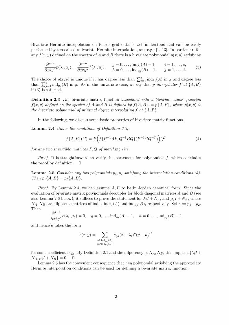
In most practically relevant instances of the univariate case, the eigenvalues of A arecontained in a domain of holomorphy of f and therefore $A is connected. This appears tohappen less frequently for bivariate holomorphic functions. As a typical example, considerf(x, y) = 1/(x#y) and let the eigenvalues of A be 1/2, 1+1/2, . . . , n+1/2 while the eigenvaluesof B are 1, 2, . . . , n. Then any $A ! $B in the sense of Theorem 2.8 consists of at least n2

connected components, see also Figure 1.

0 2 4 60

1

2

3

4

5

6

Eigenvalues of A

Eig

enva

lues

of B

Figure 1: Red line: Singularities of f(x, y) = 1/(x#y). Blue squares: Set ($A'R)!($B'R)for which $A ! $B satisfies the requirements of Theorem 2.8

3 Spectral properties and composition of functions

The eigenvalues of the linear operator f{A,B} are scalars ! $ C for which there is a nonzeroC $ Cm#n such that f{A,B}(C) = !C. Equivalently, these are the eigenvalues of the

6

mn ! mn matrix M(f{A,B}), where M denotes the natural isomorphism between linearoperators on Cm#n and mn!mn matrices.

Lemma 3.1 Let !1, . . . ,!s and µ1, . . . , µt denote the eigenvalues of A and B, respectively.Then the eigenvalues of f{A,B} are given by f(!i, µj) for i = 1, . . . , s, j = 1, . . . , t.

Proof. By Definition 2.3, f{A,B} = p{A,B}, where the polynomial p(x, y) =#

ij pijxiyj

interpolates f at {A,B}. By a direct extension of the usual argument for linear matrixequations (see, e.g., [12, Thm 4.45]), the eigenvalues of

M(p{A,B}) =$

ij

pij!Bj (Ai

".

are given by p(!i, µj) = f(!i, µj).To discuss the index of f(!i, µj) as an eigenvalue of f{A,B}, the following result will turn

out to be useful.

Lemma 3.2 Let f1, f2 be holomorphic functions in the vicinity of the spectra of A,B. Thenf1{A,B} " f2{A,B} = #{A,B} with #(x, y) = f1(x, y)f2(x, y).

Proof. By an appropriate choice of contours #A and #B, Theorem 2.8 implies

!f1{A,B} " f2{A,B}

"(C) =

1

16#4

/

!A

/

!B

/

!A

/

!B

f1(x1, y1)f2(x2, y2)(x1I #A)"1(x2I #A)"1 · · ·

· · ·C(y1I #B)"1(y2I #B)"1dy2dx2dy1dx1.

Using

# 1

4#2

/

!A

/

!A

f1(x1, y1)f2(x2, y2)(x1I #A)"1(x2I #A)"1dx2dx1

=1

2#i

/

!A

f1(x, y1)f2(x, y2)(xI #A)"1dx,

see, e.g., [20, Sec 7], and an analogous formula for (y1 #B)"1(y2 #B)"1, we obtain

!f1{A,B} " f2{A,B}

"(C) = # 1

4#2

/

!B

/

!A

f1(x, y)f2(x, y)(xI #A)"1C(yI #B)"1dy dx

= #{A,B}(C).

An immediate consequence of Lemma 3.2, bivariate matrix functions evaluated at thesame arguments commute: f1{A,B}"f2{A,B} = f2{A,B}"f1{A,B}. Another consequenceis the power rule

f{A,B} " · · · " f{A,B}0 12 3d times

= fd{A,B}. (14)

Corollary 3.3 Let $ be an eigenvalue of f{A,B}. Then

ind"f{A,B} ) max4ind!A+ indµB # 1: $ = f(!, µ),! $ %(A), µ $ %(B)

5, (15)

where % denotes the set of eigenvalues of a matrix.

7

Proof. From Lemma 2.4 it is clear that we can assume without loss of generality that Aand B are already in Jordan canonical form (7). Then the matrix representation of f{A,B}becomes block diagonal with diagonal blocks

M(f{JA(!), JB(µ)}) =ind!(A)"1$

i=0

indµ(B)"1$

j=0

pij!JTB (µ)# µI

"j (!JA(!)# !I

"i,

for some coe!cients pij with p00 = f(!, µ) =: $, see (8). Defining the polynomial p(x, y) =#i+j$1

pijxiyj , we have

f{JA(!), JB(µ)}# $I = p{JA(!)# !I, JB(µ)# µI}

and therefore, by (14),

!f{JA(!), JB(µ)}# $I

"d= pd{JA(!)# !I, JB(µ)# µI}.

By the binomial theorem,

pd{JA(!)# !I, JB(µ)# µI} =$

i+j$d

qij!JTB (µ)# µI

"j (!JA(!)# !I

"i

for some coe!cients qij . A term in this sum becomes zero if i * ind!(A) or j * ind!(B),which will always be the case if d = ind!(A) + indµ(B)# 1. Hence,

ind"f{JA(!), JB(µ)} ) ind!A+ indµB # 1.

This shows the result by taking the maximum over all eigenvalue pairs !, µ that satisfy$ = f(!, µ).

In most cases of practical interest, we expect that equality holds in (15). However, thereare obvious exceptions, as the trivial example f(x, y) + 0 demonstrates.

A bivariate matrix function f{A,B} can be composed with a univariate function u(z) byapplying the usual definition of matrix function to the matrix representation M(f{A,B}).Formally, we let

u(f{A,B}) := M"1(u(M(f{A,B}))).

This definition assumes u to be defined on the spectrum of f{A,B}, for which a su!cientcondition in terms of the Jordan structures of A and B can be easily derived from (3.3): Thederivatives

u(g)!f(!i, µj)

",

i = 1, . . . , s, j = 1, . . . , t,g = 0, . . . , ind!iA+ indµjB # 2,

(16)

are assumed to exist.

Theorem 3.4 Consider a bivariate function f(x, y) defined on the spectra of square matricesA,B and a univariate function u(z) for which the derivatives (16) exist. Then

u(f{A,B}) = (u " f){A,B}. (17)

8

Proof. Since both sides of (17) are linear in u, the power rule (14) implies that the state-ment of the lemma holds for any polynomial u. Now, let the polynomial pf interpolate f at

{A,B}, and let pu be a Hermite interpolation of u satisfying p(g)u!f(!i, µj)

"= u(g)

!f(!i, µj)

"

for all i, j, g as in (16). Then

u(f{A,B}) = pu(pf{A,B}) = (pu " pf ){A,B}.

The proof is concluded if we can show that pu " pf interpolates u " f at {A,B}. By Faa diBruno’s chain rule, the mixed derivative

"g+h

"xgyhpu!pf (x, y)

"

can be expressed in terms of derivatives of pu up to order g+h and mixed partial derivativesof pf up to order g, h in x, y. Applying this chain rule to the conditions (3) for u " f , all theresulting derivatives of pu and pf are found to match those of u and f , respectively. Hence, (3)is satisfied; pu " pf indeed interpolates u " f at {A,B}.

To give some examples of Theorem 3.4, consider first the Sylvester equation AX#XBT =C or, equivalently, f{A,B}(X) = C for f(x, y) = x#y. Provided that A and B have disjointspectra, Theorem 3.4 implies that the solution X = f{A,B}"1(C) can be written as

X = fsylv{A,B}(C) with fsylv(x, y) =1

x# y.

Similarly, the solution to the Stein equation X # AXBT = C, if it exists and is unique, canbe written as

X = fstein{A,B}(C) with fstein(x, y) =1

1# xy.

As a last example, Theorem 3.4 implies the identity

!I (A+B ( I

""1/2vec(C) = fisqr{A,B}(C) with fisqr(x, y) = (x+ y)"1/2, (18)

which allows for the application of the inverse matrix square root of I ( A + B ( I withouthaving to form this matrix explicitly, see Section 5 for a more detailed discussion.

4 Frechet derivatives of univariate matrix functions

Given a su!ciently often di"erentiable univariate function f(x), the Frechet derivative of fat a matrix A in direction C is defined as

Df{A}(C) := limh%0

1

h

!f(A+ hC)# f(A)

".

The following result shows that Df{A}(C) can be interpreted as a bivariate matrix functionrepresenting the finite di"erence evaluated at A.

Theorem 4.1 Let A be a square matrix and let f be 2 · ind!A# 1 times continuously di!er-entiable at ! for every ! $ %(A). Then

Df{A}(C) = f [1]{A,AT }(C), with f [1](x, y) := f [x, y] =

6f(x)"f(y)

x"y , for x ,= y,

f &(x), for x = y.

9

Proof. For f(x) = xk, it is well known (and easy to see) that

Df{A}(C) =k$

i=1

Ak"iCAi"1 = f [1]{A,AT }(C)

with f [1](x, y) =#k

i=1 xk"iyi"1 = (xk # yk)/(x# y) for x ,= y and f [1](x, x) = f &(x). Because

of linearity, this shows the statement of the theorem for every polynomial. For the general caseof a function f satisfying the assumptions, let p be an interpolating polynomial matching thefirst 2 · ind!A#1 derivatives of f at every eigenvalue ! of A. Consider any pair of eigenvalues!, µ of A, and let

T =

)

****+

%0 1

%1. . .. . . 1

%g+h+1

,

----., %0 = · · · = %g = !, %g+1 = · · · = %g+h+1 = µ.

Then f(T ) is defined and equals p(T ) as long as 0 ) g+ h ) ind!A+ indµA# 1. A result byOpitz [24] shows that the upper triangular entries of f(T ) are the divided di"erences of f . Inparticular, the entry in the upper right corner equals

f7!, . . . ,!0 12 3g + 1 times

, µ, . . . , µ0 12 3h+ 1 times

8=

9:

;

1g!h!

#g+h

#xgyhf [x, y]

<<<x=!,y=µ

for ! ,= µ,

1(g+h)!

#g+h

#xg+h f(x)<<<x=!

for ! = µ,

which, together with f(T ) = p(T ), shows

"g+h

"xgyhp[1](!, µ) =

"g+h

"xgyhf [1](!, µ)

for all 0 ) g+h ) ind!A+indµA#1. Hence, p[1] satisfies the required interpolation conditionsand

Df{A}(C) = Dp{A}(C) = p[1]{A,AT } = f [1]{A,AT }

concludes the proof.Using Lemma 3.2 and Theorem 4.1, the trivial relation f [x, y]x#f [x, y]y = f [x, y](x#y) =

f(x)# f(y), gives – expressed in terms of the matrix A – the commutator relations

ADf{A}(C)#Df{A}(C)A = Df{A}(AC # CA) = f(A)C # Cf(A), -C $ Cn#n (19)

for any holomorphic function f , see also [3, Thm 2.1]. Najfeld and Havel [23, Thm 4.4]have obtained an expression for Df{A} from (19) for functions f that admit a power se-ries with convergence radius & and .A. < &. In [23], this expression is called “generalizeddivided di"erence matrix”, which coincides with the matrix representation of f{A,A} andthus matches the statement of Theorem 4.1. Note, however, that Theorem 4.1 imposes muchweaker conditions on f and A.

Theorem 4.1 together with Lemma 3.1 reconfirm the well-known fact that the eigenval-ues of Df{A} are given by f [!, µ] for all pairs !, µ $ %(A), see also Theorem 3.9 in [11].Lemma 2.7 and (10) yield explicit expressions for Df{A} = f [1]{A,AT } that recover an

10

expression of Horn and Johnson stated in [12, Thm 6.6.14] under stronger assumptions onthe di"erentiability of f . Note that all these explicit expressions coincide with a formula byDaleckiı and Kreın [5, 4] in the special case that A is diagonalizable, see also (21) below andTheorem 3.11 in [11].

Finally, we demonstrate the versatility of the framework of bivariate matrix functions byshowing the well-known relation

f

='A C0 A

(>=

'A Df{A}(C)0 A

((20)

under minimal conditions on f,A.

Theorem 4.2 Equation (20) holds under the assumptions of Theorem 4.1.

Proof. It is well known (and easy to show) that (20) holds for any polynomial. Setting

M =

'A C0 A

(, we clearly have ind!M ) 2 · ind!A for every ! $ %(A). Hence, for a

polynomial p interpolating the first 2 · ind!A#1 derivatives of f at !, we have p(M) = f(M).By the argument used in the proof of Theorem 4.1, p[1] interpolates f [1] at {A,AT }. Thisconcludes the proof:

f(M) = p(M) =

'p(A) p[1]{A,AT }(C)0 p(A)

(=

'f(A) f [1]{A,AT }(C)0 f(A)

(.

In comparison, Theorem 2.1 in [22] shows (20) only under the stronger assumption that fis m# 1 times continuously di"erentiable at every eigenvalue of A, where m = max{ind!A :! $ %(A)}.

By applying the Cauchy integral representation for holomorphic matrix functions, Equa-tion (20) implies a well-known integral representation for Df(A), see [27]. It is instructive torederive this representation from the Cauchy integral formulation of Theorem 2.8 applied tof [1]{A,AT }.

5 Computation of bivariate matrix functions

The purpose of this section is to provide a rather informal discussion of possible algorithmsfor computing f{A,B}(C) for medium-sized matrices A,B.

Diagonalization of A and B. Suppose that A,B are diagonalizable:

P"1AP = diag(!1, . . . ,!m), Q"1BQ = diag(µ1, . . . , µn),

and let C = P"1CQ"T . Then Lemma 2.7 implies

f{A,B}(C) = P!F " C

"QT with fij = f(!i, µj), (21)

where “"” denotes the Hadamard product. This expression is well-suited for (nearly) normalmatrices A and B but can be expected to run into numerical instabilities when P and/or Qare ill-conditioned.

11

Diagonalization of B only. The above approach can be modified if only one of the ma-trices, say B, is known to admit a well-conditioned basis of eigenvectors. Let Q"1BQ =diag(µ1, . . . , µn) and partition C = CQ"T =

7c1, . . . , cn

8. Then Lemma 2.4 and Lemma 2.6

implyf{A,B}(C) =

7y1, . . . , yn

8QT with yj = f{A, µj}(cj). (22)

Note that f{A, µj} = fµj (A) is a univariate matrix function for fµj (x) = f(x, µj). Having astable procedure for evaluating/applying fµj (A) at hand, this approach can be expected tobe significantly more robust than (21). An analogous, row-wise procedure can be performedif A is known to admit a well-conditioned basis of eigenvectors.

Taylor expansion. In the extreme case that all eigenvalues of B are nearly identical, thediagonalization of B is clearly not the preferred option but this situation can be exploited aswell. Following the approach for univariate matrix functions proposed by Kagstrom [16], seealso [6], we let µ = trace(B)/n and consider the truncated Taylor expansion

f(x, y) / f(x, µ) + (y # µ)"

"yf(x, µ) + · · ·+ 1

k!(y # µ)k

"k

"ykf(x, µ). (23)

This yields an approximation for the bivariate matrix function in terms of the univariate

functions f (0)µ (x) := f(x, µ), f (1)

µ (x) := ##yf(x, µ), . . . , f

(k)µ (x) := #k

#ykf(x, µ):

f{A,B}(C) / f (0)µ (A)C + f (1)

µ (A)C(B # µI) + · · ·+ 1

k!f (k)µ (A)C(B # µI)k. (24)

Since B has all eigenvalues close to µ, one can expect that k need not be chosen very large toobtain good accuracy, see [6, 11, 16, 21] for discussions. Compared to (22), formula (24) has

the requirement that not only f (0)µ but also the derivatives f (1)

µ , . . . , f (k)µ need to be evaluated

at A. Without going into implementation details, we only mention that if the Schur-Parlettalgorithm [6] is used for this purpose then the mixed partial derivatives of f need to beavailable, which could be considered a not too unreasonable requirement.

Block diagonalization of B only. Diagonalization and Taylor expansion can be combinedin an obvious manner by considering a block diagonalization of B:

Q"1BQ = diag!B11, . . . , Btt

"(25)

such that Q is well-conditioned and the eigenvalues of each diagonal block Bjj are nearlyidentical. Methods for performing such a decomposition reliably are a subtle matter and havebeen discussed, e.g., in [6, 9, 25]. Assuming (25) is available,

f{A,B}(C) =7Y1, . . . , Yn

8QT with Yj = f{A,Bjj}(Cj),

where C = CQ"T =7C1, . . . , Cn

8is partitioned in accordance with Q"1BQ. In e"ect, each

block column Yj can be computed by means of (24).An analogous, block row-wise procedure can be derived if it is preferable to block diago-

nalize A.

12

Summary. As noted in [6, 11], algorithms for evaluating univariate matrix functions basedon block diagonalization have their deficiencies. In particular, to obtain a very well-conditionedQ, the spectrum of the diagonal blocks can often not be chosen very narrow. Consequently,to yield good accuracy, a large value of k needs to be chosen in the truncated Taylor ex-pansion (24). The Schur-Parlett algorithm [6, 25] has been demonstrated to allow for morenarrow block diagonal spectra and is therefore preferred over block diagonalization. It wouldbe desirable to have a bivariate analogue of this algorithm, which ideally would reduceto the well-known Bartels-Stewart algorithm for Sylvester matrix equations if applied tof(x, y) = 1/(x#y). Unfortunately, the derivation of such an analogue appears to be di!cult.

It should be stressed that there are far better algorithms available for the two mostimportant special cases of matrix functions; we refer to [15] for linear matrix equations andto [11] for matrix Frechet derivatives.

6 Extension to multivariate functions

For the sake of clarity, the focus of this paper has been on bivariate matrix functions. However,the extension to arbitrary multivariate functions is rather simple.

First, consider a d-variate polynomial

p(x1, . . . , xd) =s1$

i1=1

· · ·sd$

id=1

pi1,...,idxi11 · · ·xidd =

$

i'Ipix

i,

where we used the usual multiindex notation and I = [1, s1]! · · ·! [1, sd]. For the evaluationof p at d matrices A1 $ Cn1#n1 , . . . , Ad $ Cnd#nd , we propose to define

p{A1, . . . , Ad}(C) :=$

i'IpiC !1 A

i11 !2 A

i22 · · ·!d A

idd ,

where C $ Cn1#n2#···#nd is a tensor of order d and !j denotes the j-mode multiplication of atensor with a matrix [7, 2]. This matches (2) for d = 2 since Ai1

1 C(AT2 )

i2 = C !1 Ai11 !2 A

i22 .

For a general function f(x1, . . . , xd), tensor Hermite interpolation yields a polynomialp(x1, . . . , xd) satisfying

"|g|

"xgp(!1, . . . ,!d) =

"|g|

"xgf(!1, . . . ,!d),

g = (g1, . . . , gd),gk = 0, . . . , ind!k

(Ak)# 1, k = 1, . . . , d,(26)

for every tuple of eigenvalues !1 $ %(A1), . . . ,!d $ %(Ad), provided of course that all requiredmixed derivatives of f exist and are continuous. The d-variate matrix function associatedwith f can then be defined as f{A1, . . . , Ad} := p{A1, . . . , Ad}, which is a linear operator onCn1#n2#···#nd .

Mutatis mutandis, all results presented for bivariate matrix functions can be expected toadmit d-variate extensions. For example, if f is holomorphic on an open set $ = $1!· · ·!$d,with %(Ak) & $k, and continuous on $, the d-variate analogue of the Cauchy integral formulaof Theorem 2.8 becomes

f{A1, . . . , Ad}(C) =1

(2#i)d

/

!1

· · ·/

!d

f(x1, . . . , xd)C !1 (x1I #A1)"1 · · ·!d (xdI #Ad)

"1dx,

13

where #k is the contour of $k.The multivariate matrix function for f(x1, . . . , xd) = 1/(x1+ · · ·+xd) can be used to solve

discretizations of separable partial di"erential equations, see [8, 19]. We are not aware of anyother applications.

7 Conclusions and Outlook

The definition of bivariate matrix function proposed in this paper has resulted in the unifica-tion and (mild) improvements of some existing results for linear matrix equations and matrixFrechet derivatives. It remains to be seen whether other applications fit into our framework.

This paper has only discussed basic results and briefly touched computational aspects.There is evidence that the concept of bivariate matrix functions may o"er a more abstractview and possibly new insights for a variety of other, more advanced results. First, existingKrylov subspace methods for Lyapunov matrix equations [14, 26] could be extended andviewed as bivariate polynomial matrix approximations. Second, an analogue of Theorem 4.1for Frechet derivatives of bivariate matrix functions could lead to a more e!cient way tocompute condition numbers for linear matrix equations, cf. [10, Sec. 16.3].

References

[1] A. C. Ahlin. A bivariate generalization of Hermite’s interpolation formula. Math. Comp.,18:264–273, 1964.

[2] B. W. Bader and T. G. Kolda. Algorithm 862: MATLAB tensor classes for fast algorithmprototyping. ACM Trans. Math. Software, 32(4):635–653, 2006.

[3] R. Bhatia and K. B. Sinha. Derivations, derivatives and chain rules. Linear AlgebraAppl., 302/303:231–244, 1999.

[4] Ju. L. Daleckiı. Di"erentiation of non-Hermitian matrix functions depending on a pa-rameter. Amer. Math. Soc. Transl., Series 2, 47:73–87, 1965.

[5] Ju. L. Daleckiı and S. G. Kreın. Integration and di"erentiation of functions of Hermitianoperators and applications to the theory of perturbations. Amer. Math. Soc. Transl.,Series 2, 47:1–30, 1965.

[6] P. I. Davies and N. J. Higham. A Schur–Parlett algorithm for computing matrix func-tions. SIAM J. Matrix Anal. Appl., 25(2):464–485, 2003.

[7] L. De Lathauwer, B. De Moor, and J. Vandewalle. A multilinear singular value decom-position. SIAM J. Matrix Anal. Appl., 21(4):1253–1278, 2000.

[8] L. Grasedyck. Existence and computation of low Kronecker-rank approximations forlarge linear systems of tensor product structure. Computing, 72(3-4):247–265, 2004.

[9] M. Gu. Finding well-conditioned similarities to block-diagonalize nonsymmetric matricesis NP-hard. Journal of Complexity, 11(3):377–391, September 1995.

[10] N. J. Higham. Accuracy and Stability of Numerical Algorithms. SIAM, Philadelphia,PA, second edition, 2002.

14

[11] N. J. Higham. Functions of matrices. Society for Industrial and Applied Mathematics(SIAM), Philadelphia, PA, 2008.

[12] R. A. Horn and C. R. Johnson. Topics in Matrix Analysis. Cambridge University Press,Cambridge, 1991.

[13] E. Isaacson and H. B. Keller. Analysis of numerical methods. Dover Publications Inc.,New York, 1994. Corrected reprint of the 1966 original.

[14] I. M. Jaimoukha and E. M. Kasenally. Krylov subspace methods for solving large Lya-punov equations. SIAM J. Numer. Anal., 31:227–251, 1994.

[15] I. Jonsson and B. Kagstrom. Recursive blocked algorithm for solving triangular systems.I. one-sided and coupled Sylvester-type matrix equations. ACM Trans. Math. Software,28(4):392–415, 2002.

[16] B. Kagstrom. Numerical computation of matrix functions. Report UMINF-58.77, De-partment of Information Processing, University of Umea, Sweden, July 1977.

[17] S. G. Krantz. Function Theory of Several Complex Variables. John Wiley & Sons Inc.,New York, 1982.

[18] M. G. Kreın. Lektsii po teorii ustoichivosti reshenii di!erentsialnykh uravnenii v Ba-nakhovom prostranstve. Izdat. Akad. Nauk Ukrain. SSR, Kiev, 1964.

[19] D. Kressner and C. Tobler. Krylov subspace methods for linear systems with tensorproduct structure. SIAM J. Matrix Anal. Appl., 31(4):1688–1714, 2010.

[20] P. Lancaster. Explicit solutions of linear matrix equations. SIAM Rev., 12:544–566, 1970.

[21] R. Mathias. Approximation of matrix-valued functions. SIAM J. Matrix Anal. Appl.,14(4):1061–1063, 1993.

[22] R. Mathias. A chain rule for matrix functions and applications. SIAM J. Matrix Anal.Appl., 17(3):610–620, 1996.

[23] I. Najfeld and T. F. Havel. Derivatives of the matrix exponential and their computation.Advances in Applied Mathematics, 16:321–375, 1995.

[24] G. Opitz. Steigungsmatrizen. Z. Angew. Math. Mech., 44:T52–T54, 1964.

[25] B. N. Parlett and K. C. Ng. Development of an accurate algorithm for exp(Bt). TechnicalReport PAM-294, Center for Pure and Applied Mathematics, University of California,Berkeley, August 1985.

[26] Y. Saad. Numerical solution of large Lyapunov equations. In Signal processing, scatteringand operator theory, and numerical methods (Amsterdam, 1989), volume 5 of Progr.Systems Control Theory, pages 503–511. Birkhauser Boston, Boston, MA, 1990.

[27] E. Stickel. On the Frechet derivative of matrix functions. Linear Algebra Appl., 91:83–88,1987.

15

Research Reports

No. Authors/Title

10-22 D. KressnerBivariate matrix functions

10-21 C. Jerez-Hanckes and J.-C. NedelecVariational forms for the inverses of integral logarithmic operators overan interval

10-20 R. AndreevSpace-time wavelet FEM for parabolic equations

10-19 V.H. Hoang and C. SchwabRegularity and generalized polynomial chaos approximation of paramet-ric and random 2nd order hyperbolic partial di!erential equations

10-18 A. Barth, C. Schwab and N. ZollingerMulti-Level Monte Carlo Finite Element method for elliptic PDE’s withstochastic coe"cients

10-17 B. Kagstrom, L. Karlsson and D. KressnerComputing codimensions and generic canonical forms for generalizedmatrix products

10-16 D. Kressner and C. ToblerLow-Rank tensor Krylov subspace methods for parametrized linearsystems

10-15 C.J. GittelsonRepresentation of Gaussian fields in series with independent coe"cients

10-14 R. Hiptmair, J. Li and J. ZouConvergence analysis of Finite Element Methods for H(div;#)-ellipticinterface problems

10-13 M.H. Gutknecht and J.-P.M. ZemkeEigenvalue computations based on IDR

10-12 H. Brandsmeier, K. Schmidt and Ch. SchwabA multiscale hp-FEM for 2D photonic crystal band

10-11 V.H. Hoang and C. SchwabSparse tensor Galerkin discretizations for parametric and randomparabolic PDEs. I: Analytic regularity and gpc-approximation

10-10 V. Gradinaru, G.A. Hagedorn, A. JoyeExponentially accurate semiclassical tunneling wave functions in one di-mension