Matrix Analysis,Polya frequency functions, andPreservers of (Total) Positivity

Apoorva Khare

Indian Institute of Science

1. Introduction 3

1. Introduction

This text arose out of the course notes for Math 341: Matrix Analysis and Positivity, aone-semester course offered in Spring 2018 and Fall 2019 at the Indian Institute of Science(IISc). Owing to the subsequent inclusion of additional topics, the text has now grown tocover roughly a two-semester course in analysis and matrix positivity preservers – or, morebroadly, composition operators preserving various kinds of positive kernels. Thus in thistext, we briefly describe some notions of positivity in matrix theory, followed by our mainfocus: a detailed study of the operations that preserve these notions (and, in the process,an understanding of some aspects of real functions). Several different notions of positivity inanalysis, studied for classical and modern reasons, are touched upon in the text:

• Positive semidefinite and positive definite matrices.• Entrywise positive matrices.• A common strengthening of the first two notions, which involves totally positive (TP )

and totally non-negative (TN) matrices.• Settings somewhat outside matrix theory. For instance, consider discrete data asso-

ciated with positive measures on locally compact abelian groups G. E.g., for G = R,one obtains moment sequences, which are intimately related to positive semidefiniteHankel matrices. For G = S1, the circle group, one obtains Fourier–Stieltjes se-quences, which are connected to positive semidefinite Toeplitz matrices. (See worksof Caratheodory, Hamburger, Hausdorff, Herglotz, and Stieltjes, among others.)• More classically, functions and kernels with positivity structures have long been stud-

ied in analysis, including on locally compact groups and metric spaces (see Bochner,Schoenberg, von Neumann, Polya). Distinguished examples include positive definitefunctions and Polya frequency functions and sequences.

The text begins by discussing the above notions, focussing on their properties and someresults in matrix theory. The next two parts then study, in detail, the preservers of severalof these notions of positivity. Among other things, this journey involves going throughmany beautiful classical results by leading experts in analysis during the first half of thetwentieth century. Apart from also covering several different tools required in proving theseresults, an interesting outcome also is that several classes of “positive” matrices repeatedly gethighlighted by way of studying positivity preservers – these include generalized Vandermondematrices, Hankel moment matrices and kernels, and Toeplitz kernels on the line or the integers(aka Polya frequency functions and sequences).

In this text, we will study the post-composition transforms that preserve (total) positivityon various classes of kernels. When the kernel has finite domain – i.e., is a matrix – thenthis amounts to studying entrywise preservers of various notions of positivity. The questionof why entrywise calculus was studied – as compared to the usual holomorphic functionalcalculus – has a rich and classical history in the analysis literature, beginning with thework of Schoenberg, Rudin, Loewner, and Horn (these results are proved in Part 3 of thetext), but also drawing upon earlier works of Menger, Schur, Bochner, and others. (Infact, the entrywise calculus was introduced, and the first such result proved, by Schur in1911.) Interestingly, this entrywise calculus also arises in modern-day applications fromhigh-dimensional covariance estimation; we elaborate on this in Section 13.1, and briefly alsoin Section 14. Furthermore, this evergreen area of mathematics continues to be studied in theliterature, drawing techniques from – and also contributing to – symmetric function theory,statistics and graphical models, combinatorics, and linear algebra (in addition to analysis).

4 1. Introduction

As a historical curiosity, the course and this text arose in a sense out of research car-ried out in significant measure by mathematicians at Stanford University (including theirstudents) over the years. This includes Loewner, Karlin, and their students: FitzGerald,Horn, Micchelli, and Pinkus. Less directly, there was also Katznelson, who had previouslyworked with Helson, Kahane, and Rudin, leading to Rudin’s strengthening of Schoenberg’stheorem. (Coincidentally, Polya and Szego, who made the original observation on entrywisepreservers of positivity using the Schur product theorem, were again colleagues at Stanford.)On a personal note, the author’s contributions to this area also have their origins in his timespent at Stanford University, collaborating with Alexander Belton, Dominique Guillot, MihaiPutinar, Bala Rajaratnam, and Terence Tao (though the collaboration with the last-namedcolleague was carried out almost entirely at IISc).

We now discuss the course, the notes that led to this text, and their mathematical contents.The notes were scribed by the students taking the course in Spring 2018 at IISc, followed byextensive “homogenization” by the author – and, in several sections, addition of material.Each section was originally intended to cover the notes of roughly one 90-minute lecture, oroccasionally two; that said, some material has subsequently been moved around for logical,mathematical, and expositional reasons. The notes, and the course itself, require an under-standing of basic linear algebra and analysis, with a bit of measure theory as well. Beyondthese basic topics, we have tried to keep these notes as self-contained as possible, with fullproofs. To that end, we have included proofs of “preliminary” results, including:

(i) results of Schoenberg, Menger, von Neumann, Frechet, and others connecting metricgeometry and positive definite functions to matrix positivity;

(ii) results in Euclidean geometry, including on triangulation, Heron’s formula for thearea of a triangle, and connecting Cayley–Menger matrices to simplicial volumes;

(iii) Boas–Widder and Bernstein’s theorems on functions with positive forward differences;(iv) Sierpinsky’s result: mid-convexity and measurability imply continuity;(v) an extension to normed linear spaces, of (a special case of) a classical result of Os-

trowski on mid-convexity and local boundedness implying continuity;(vi) Whitney’s density of totally positive matrices inside totally non-negative matrices;(vii) Descartes’ rule of signs – several variants;(viii) a follow-up to Descartes, by Laguerre, on variation diminution in power series, and

its follow-up by Fekete involving Polya frequency sequences;(ix) Fekete’s result on totally positive matrices via positive contiguous minors;(x) (on a related note:) results on real and complex polynomials, their “compositions”,

and zeros of these: by Gauss–Lucas, Hermite–Kakeya–Obrechkoff, Hermite–Biehler,Routh–Hurwitz, Hermite–Poulain, Laguerre, Malo, Jensen, Schur, Weisner, de Bruijn,and Polya;

(xi) a detailed sketch of Polya and Schur’s characterizations of multiplier sequences;(xii) Mercer’s lemma, identifying positive semidefinite kernels with kernels of positive type;

(xiii) Perron’s theorem for matrices with positive entries (the precursor to Perron–Frobenius);(xiv) compound matrices and Kronecker’s theorem on their spectra;(xv) Sylvester’s criterion and the Schur product theorem on positive (semi)definiteness

(also, the Jacobi formula);(xvi) the Jacobi complementary minor formula;

(xvii) the Rayleigh–Ritz theorem;(xviii) a special case of Weyl’s inequality on eigenvalues;(xix) matrix identities by Andreief and Cauchy–Binet, and a continuous generalization;

1. Introduction 5

(xx) the discreteness of zeros of real analytic functions (and a sketch of the continuity ofroots of complex polynomials); and

(xxi) the equivalence of Cauchy’s and Littlewood’s definitions of Schur polynomials (andof the Jacobi–Trudi and von Nagelsbach–Kostka identities) via Lindstrom–Gessel–Viennot bijections.

Owing to considerations of time, we had to leave out some proofs. These include proofsof theorems by Hamburger/Hausdorff/Stieltjes, Fubini, Tonelli, Cauchy, Montel, Morera,and Hurwitz; a Schur positivity phenomenon for ratios of Schur polynomials; Lebesgue’sdominated convergence theorem; as well as the closure of real analytic functions under com-position. Most of these can be found in standard textbooks in mathematics. We also omitthe proofs of several classical results on Laplace transforms and Polya frequency functions,found in textbooks, in papers by Schoenberg and his co-authors, and in Karlin’s compre-hensive monograph on total positivity. Nevertheless, as the previous and current paragraphsindicate, these notes cover many classical results by past experts and acquaint the reader witha variety of tools in analysis (especially the study of real functions) and in matrix theory –many of these tools are not found in more “traditional” courses on these subjects.

This text is broadly divided into six parts, with detailed bibliographic notes following eachpart. In Part 1, the key objects of interest – namely, positive semidefinite / totally positive/ totally non-negative matrices – are introduced, together with some basic results as well assome important classes of examples. (The analogous kernels are also studied.) In Part 2, webegin the study of functions acting entrywise on such matrices, and preserving the relevantnotion of positivity. Here, we will mostly restrict ourselves to studying power functions thatact on various sets of matrices of a fixed size. This is a long-studied question, including byBhatia, Elsner, Fallat, FitzGerald, Hiai, Horn, Jain, Johnson, and Sokal; as well as by theauthor in collaboration with Guillot and Rajaratnam. In particular, an interesting highlightis the construction by Jain of individual (pairs of) matrices, which turn out to encode theentire set of entrywise powers preserving Loewner positivity, monotonicity, and convexity.We also obtain certain necessary conditions on general entrywise functions that preservepositivity, including multiplicative mid-convexity and continuity, as well as a classification ofall functions preserving total non-negativity or total positivity in each fixed dimension. Weexplain some of the modern motivations, and we end with some unsolved problems.

Part 3 deals with some of the foundational results on matrix positivity preservers. Aftermentioning some of the early history – including work by Menger, Frechet, Bochner, andSchoenberg – we classify the entrywise functions that preserve positive semidefiniteness (=positivity) in all dimensions, or total non-negativity on Hankel matrices of all sizes. This isa celebrated result of Schoenberg – later strengthened by Rudin – which is a converse to theSchur product theorem, and we prove a stronger version by using a rank-constrained test set.The proof given in these notes is different from the previous approaches of Schoenberg andRudin, is essentially self-contained, and uses relatively less sophisticated machinery comparedto the works of Schoenberg and Rudin. Moreover, it first proves a variant by Vasudeva formatrices with only positive entries, and it lends itself to a multivariate generalization (whichwill not be covered here). The starting point of these proofs is a necessary condition forentrywise preservers in a fixed dimension, proved by Loewner (and Horn) in the late 1960s.To this day, this result remains essentially the only known condition in a fixed dimensionn ≥ 3, and a proof of a (rank-constrained, as above) stronger version is also provided in thesenotes. In addition to techniques and ingredients introduced by the above authors, the text

6 1. Introduction

also borrows from the author’s joint work with Belton, Guillot, and Putinar. This part endswith several appendices:

(1) The first appendix covers a result by Boas and Widder, which shows a converse “meanvalue theorem” for divided differences.

(2) We next cover recent work by Vishwakarma on an “off-diagonal” variant of the posi-tivity preserver problem.

(3) The third and fourth appendices classify preservers of Loewner positivity, monotonic-ity, and convexity on “dimension-free matrices”, or on kernels over infinite domains.

(4) The fifth appendix explores the theme of Euclidean distance geometry, with a focuson some classical results by Menger.

In Parts 4 and 5, we formulate the preserver problem in analysis terms, using compositionoperators on kernels. This allows one to consider such questions not only for matrices of afixed or arbitrary size, but also over more general, infinite domains. It also makes available foruse, the powerful analysis machinery developed by Bernstein, Polya, Schoenberg, Widder, andothers. Thus in Part 5, we provide characterizations of such composition operators preservingtotal positivity or non-negativity on structured kernels – specifically Toeplitz kernels onvarious sub-domains of R. Two distinguished classes of such kernels are Polya frequencyfunctions and Polya frequency sequences, i.e., Toeplitz kernels on R×R and Z×Z, respectively.

Before solving the preserver problem in this paradigm, we begin by developing some of theresults by Schoenberg and others on Polya frequency functions and sequences. In fact webegin even more classically: with a host of root-location results for zeros of real and complexpolynomials, which motivated the study of the Laguerre–Polya class of entire functions andthe Polya–Schur classification of multiplier sequences. After presenting these, we brieflydiscuss modern offshoots of the Laguerre–Polya–Schur program, followed by Schoenberg’sresults. (Similarly, in the next part we also briefly discuss the Wallach set in representationtheory and probability.)

In Part 5, we return to the question studied in Part 2 above, of classifying the preserversof all TN or TP kernels, on X × Y for arbitrary totally ordered sets X,Y . Here we providea complete resolution of this question. In a sense, the total positivity preserver problemis the culmination of all that has come before in this text; it uses many of the tools andtechniques from the previous parts. These include (i) Vandermonde kernels, TP kernelcompletions of 2×2 matrices, and Fekete’s result, from Part 1; (ii) entrywise powers preservingpositivity (via a trick of Jain to use Toeplitz cosine matrices), and the classification of total-positivity preservers in finite dimension, from Part 2; (iii) the stronger Vasudeva theoremclassifying entrywise positivity preservers on low-rank Hankel matrices, from Part 3; and(iv) preservers of Toeplitz kernels, including of Polya frequency functions and sequences,from Part 4. We also develop as needed, set-theoretic tools and Whitney-type density results– as well as understanding the structure and preservers of continuous Hankel kernels definedon an interval. This latter requires results of Mercer, Bernstein, Hamburger, and Widder.

We remark that Part 4 contains – in addition to theorems found e.g. in Karlin’s book – veryrecent results from 2020+ on Polya frequency functions (and not merely their preservers),which in particular are not found in previous treatments of the subject. To name a few:

• a characterization of Polya frequency functions of order p, for any p ≥ 3;• strengthenings of multiple results of Karlin (1955) and of Schoenberg (1964);• a converse to the same result of Karlin (1955);• a critical exponent phenomenon in total positivity;

1. Introduction 7

• a closer look at a multiparameter family of density functions introduced by Hirschmanand Widder (1949); and• a connection between Polya frequency functions and the Riemann hypothesis.

(Similarly, Part 2 of this text contains recent results on totally non-negative/positive matrices,which are not found in earlier books on total positivity.) Thus, in a sense Parts 4 and 5 canbe viewed as “one possible sequel” to Karlin’s book and to the body of work by Schoenbergon Polya frequency functions, since they present novel material on these classes of functions,then use the “structural” results by the aforementioned authors about various families ofToeplitz kernels to classify the preservers of various sub-families of these objects. In additionto results of Schoenberg and his coauthors, as well as an authoritative survey of these results,compiled in Karlin’s majestic monograph, both parts borrow from the author’s 2020 works(one with Belton, Guillot, and Putinar).

In the final Part 6, we return to the study of entrywise functions preserving positivity ina fixed dimension. This is a challenging problem – it is still open in general, even for 3 × 3matrices – and we restrict ourselves in this part to studying polynomial preservers. Accordingto the Schur product theorem (1911), if the polynomial has all non-negative coefficients, thenit is easily seen to be a preserver; but, interestingly, until 2016 not a single example wasknown of any other entrywise polynomial preserver of positivity in a fixed dimension n ≥ 3.Very recently, this question has been answered to some degree of satisfaction by the author,in collaboration first with Belton, Guillot, and Putinar, and subsequently with Tao. The textends by covering some of this recent progress, and it comes back full circle to Schur throughsymmetric function theory.

A quick note on the logical structure: Parts 1–5 are best read sequentially; note thatsome sections do not get used later in the text, e.g. Sections 8 and 31, and the Appendices.That said, Part 4, which involves non-preserver results on Polya frequency functions andsequences, can be read from scratch, requiring only Sections 6 and 12.1 and Lemma 26.3 aspre-requisites. The final Part 6 can be read following Section 9 (also see the Schoenberg–Rudin theorem 16.2 and the Horn–Loewner theorem 17.1). We also point out the occurrenceof Historical notes and Further questions, which serve to acquaint the reader with pastwork(er)s as well as related areas; and possible avenues for future work – and which can beaccessed from the Index at the end. (See also the Bibliographic notes at the end of each partof the text.)

To conclude, thanks are owed to the scribes (listed below), as well as to Alexander Bel-ton, Shabarish Chenakkod, Projesh Nath Choudhury, Julian R. D’Costa, Dominique Guillot,Prakhar Gupta, Roger A. Horn, Sarvesh Ravichandran Iyer, Poornendu Kumar, GadadharMisra, Frank Oertel, Aaradhya Pandey, Vamsi Pritham Pingali, Paramita Pramanick, MihaiPutinar, Shubham Rastogi, Aditya Guha Roy, Siddhartha Sahi, Kartik Singh, Naren Sun-daravaradan, G.V. Krishna Teja, Akaki Tikaradze, Raghavendra Tripathi, Prateek KumarVishwakarma, and Pranjal Warade for helpful suggestions that improved the text. I am, ofcourse, deeply indebted to my collaborators for their support and all of their research effortsin positivity – but also for many stimulating discussions, which helped shape my thinkingabout the field as a whole and the structure of this text in particular. Finally, I am gratefulto the University Grants Commission (UGC, Government of India), the Science and Engi-neering Research Board (SERB) and the Department of Science and Technology (DST) ofthe Government of India, the Infosys Foundation, and the Tata Trusts – for their supportthrough a CAS-II grant, through a MATRICS grant and the Ramanujan and Swarnajayanti

8 1. Introduction

Fellowships, through a Young Investigator Award, and through their Travel Grants, respec-tively.

Department of Mathematics, Indian Institute of Science& Analysis and Probability Research Group

Bangalore, India

1. Introduction 9

List of scribes: Each section contains material originally covered in a 90-minute lecture,and subsequently augmented by the author. These lectures (in Spring 2018) did not coverSections 4, 8 in Part 1, Section 15 in Part 2, the entirety of Parts 4 and 5, and the Appendices.The text also includes two sets of “general remarks” by the author; see Sections 13.1 and 14.

Part 1: Preliminaries

(1) January 03: (Much of the above text.)(2) January 08: Sarvesh Iyer(3) January 10: Prateek Kumar Vishwakarma(4) Apoorva Khare(5) January 17: Prakhar Gupta(6) January 19: Pranjal Warade(7) January 24: Swarnalipa Datta, and Apoorva Khare(8) Apoorva Khare

Part 2: Entrywise powers preserving (total) positivity in a fixed dimension

(9) January 31: Raghavendra Tripathi(10) February 02: Pabitra Barman(11) February 07: Kartick Ghosh(12) February 09: K. Philip Thomas (and Feb 14: Pranab Sarkar), and Apoorva Khare(13) February 28: Ratul Biswas (with an introduction by Apoorva Khare)(14) March 02: Prateek Kumar Vishwakarma (with remarks by Apoorva Khare)(15) Apoorva Khare

Part 3: Entrywise functions preserving positivity in all dimensions

(16) February 14, 16: Pranab Sarkar, Pritam Ganguly, and Apoorva Khare(17) March 07: Shubham Rastogi(18) March 09: Poornendu Kumar, Sarvesh Iyer, and Apoorva Khare(19) March 14: Poornendu Kumar and Shubham Rastogi(20) March 16: Lakshmi Kanta Mahata and Kartick Ghosh(21) March 19, 21: Kartick Ghosh, Swarnalipa Datta, and Apoorva Khare(22) March 23: Sarvesh Iyer and Raghavendra Tripathi(23) Appendix A: Poornendu Kumar, Shubham Rastogi, and Apoorva Khare(24) Appendix B: Prateek Kumar Vishwakarma and Apoorva Khare

(25–27) Appendices C–E: Apoorva Khare

Part 4: Polya frequency functions and sequences

(28–35) Apoorva Khare

Part 5: Composition operators preserving totally positive kernels

(36–40) Apoorva Khare

Part 6: Entrywise polynomials preserving positivity in a fixed dimension

(41) March 26: Prakhar Gupta, Pranjal Warade, and Apoorva Khare(42) March 28: Ratul Biswas and K. Philip Thomas(43) April 02: Pritam Ganguly and Pranab Sarkar(44) April 11: Pabitra Barman, Lakshmi Kanta Mahata, and Apoorva Khare(45) Appendix F: Apoorva Khare

Contents

1. Introduction 3

Part 1: Preliminaries 15

2. The cone of positive semidefinite matrices. Examples. Schur complements. 153. Schur product theorem. Totally positive/non-negative matrices. Examples. 234. Fekete’s result. Hankel moment matrices are TN . Hankel positive semidefinite

and TN matrices. 295. Generalized Vandermonde matrices. Cauchy–Binet formula and its generalization. 336. Hankel moment matrices are TP . Andreief’s identity. Density of TP in TN . 377. (Non-)Symmetric TP completion problems. 418. Theorems of Perron and Kronecker. Spectra of TP and TN matrices. 45Bibliographic notes and references 50

Part 2: Entrywise powers preserving (total) positivity in a fixed dimension 53

9. Entrywise powers preserving positivity in a fixed dimension: I. 5310. Entrywise powers preserving total positivity: I. 5711. Entrywise powers preserving total positivity: II. 6112. Entrywise functions preserving total positivity. Mid-convex implies continuity.

The test set of Hankel TN matrices. 6513. Entrywise powers (and functions) preserving positivity: II. Matrices with zero

patterns. 7514. Entrywise powers preserving positivity: III. Chordal graphs. Loewner

monotonicity and super-additivity. 8115. Loewner convexity. Single matrix encoders of entrywise power-preservers of

Loewner properties. 87Bibliographic notes and references 95

Part 3: Entrywise functions preserving positivity in all dimensions 99

16. History – Schoenberg’s theorem. Rudin, Herz, Vasudeva. Metric geometry,positive definite functions, spheres, and correlation matrices. 99

17. Horn’s thesis: a determinant calculation. Proof for smooth functions. 11118. The stronger Horn–Loewner theorem. Mollifiers. 11519. The stronger Vasudeva and Schoenberg theorems. Bernstein’s theorem. Moment

sequence transforms. 11920. Proof of stronger Schoenberg Theorem: I. Continuity. The positivity-certificate

trick. 12521. Proof of stronger Schoenberg Theorem: II. Smoothness implies real analyticity. 13122. Proof of stronger Schoenberg Theorem: III. Complex analysis. Further remarks. 13523. Appendix A: The Boas–Widder theorem on functions with positive differences. 13724. Appendix B: Functions acting outside forbidden diagonal blocks. Dimension-free

non-absolutely-monotonic preservers. 14725. Appendix C. Preservers of positivity on kernels. 15326. Appendix D. Preservers of Loewner monotonicity and convexity on kernels. 15727. Appendix E. Menger’s results and Euclidean distance geometry. 163Bibliographic notes and references 171

12 1. Introduction

Part 4: Polya frequency functions and sequences 175

28. Totally non-negative functions of finite order. 17529. Polya frequency functions. The variation diminishing and sign non-reversal

properties. Single-vector characterizations of TP and TN matrices. 18330. Polya frequency sequences and their generating functions. 19731. Complement: Root-location results and TN Hurwitz matrices 20932. Examples of Polya frequency functions: Laplace transform, convolution. 21533. History – The Laguerre–Polya–Schur program: multiplier sequences and entire

functions. Modern results. 22134. Schoenberg’s results on Polya frequency functions. 23535. Further one-sided examples: The Hirschman–Widder densities. Discontinuous

PF functions. 241Bibliographic notes and references 242

Part 5: Composition operators preserving totally positive kernels 247

36. Critical exponent for powers preserving TNp. The Jain–Karlin–Schoenbergkernel. 247

37. Preservers of Polya frequency functions. 25138. Preservers of Polya frequency sequences. 25339. Preservers of TP Hankel kernels. 25540. Total positivity preservers: All kernels. 263Bibliographic notes and references 264

Part 6: Entrywise polynomials preserving positivity in a fixed dimension 267

41. Entrywise polynomial preservers. Horn–Loewner type necessary conditions.Classification of sign patterns. 267

42. Polynomial preservers for generic rank-one matrices. Schur polynomials. 27343. First-order approximation / leading term of Schur polynomials. From rank-one

matrices to all matrices. 27944. Exact quantitative bound: monotonicity of Schur ratios. Real powers and power

series. 28345. Polynomial preservers on matrices with real or complex entries. Complete

homogeneous symmetric polynomials. 29146. Appendix F: Cauchy’s and Littlewood’s definitions of Schur polynomials. The

(dual) Jacobi–Trudi identity and Lindstrom–Gessel–Viennot bijections. 299Bibliographic notes and references 304

References 305Index 319Index 319

Part 1:Preliminaries

2. The cone of positive semidefinite matrices. Examples. Schur complements. 15

Part 1: Preliminaries

2. The cone of positive semidefinite matrices. Examples. Schur complements.

A kernel is a function K : X × Y → R. Broadly speaking, the goal of this text is tounderstand: Which functions F : R→ R, when applied to kernels with some notionof positivity, preserve that notion? To do so, we first study the test sets of such kernelsK themselves, and then the post-composition operators F that preserve these test sets. Webegin by understanding such kernels when the domains X,Y are finite, i.e., matrices.

In this text, we will assume familiarity with linear algebra and a first course in calcu-lus/analysis. To set notation: an uppercase letter with a two-integer subscript (such as Am×n)represents a matrix with m rows and n columns. If m,n are clear from context or unim-portant, then they will be omitted. Three examples of real matrices are 0m×n,1m×n, Idn×n,which are the (rectangular) matrix consisting of all zeros, all ones, and the identity matrix,respectively. The entries of a matrix A will be denoted aij , ajk, etc. Vectors are denoted bylowercase letters (occasionally in bold), and are columnar in nature. All matrices, unless spec-ified otherwise, are real; and similarly, all functions, unless specified otherwise, are definedon – and take values in – Rm for some m ≥ 1. As is standard, we let C,R,Q,Z,N denote thecomplex numbers, reals, rationals, integers, and positive integers respectively. Given S ⊂ R,let S≥0 := S ∩ [0,∞).

2.1. Preliminaries. We begin with several basic definitions.

Definition 2.1. A matrix An×n is said to be symmetric if ajk = akj for all 1 ≤ j, k ≤ n.

A real symmetric matrix An×n is said to be positive semidefinite) if the real number xTAxis non-negative for all x ∈ Rn – in other words, the quadratic form given by A is positivesemidefinite. If, furthermore, xTAx > 0 for all x 6= 0 then A is said to be positive definite.Denote the set of (real symmetric) positive semidefinite matrices by Pn.

We state the spectral theorem for symmetric (i.e., self-adjoint) operators without proof.

Theorem 2.2 (Spectral theorem for symmetric matrices). For An×n a real symmetric matrix,A = UTDU for some orthogonal matrix U (i.e., UTU = Id) and real diagonal matrix D. Dcontains all the eigenvalues of A (counting multiplicities) along its diagonal.

As a consequence, A =∑n

j=1 λjvjvTj , where each vj is an eigenvector for A with real

eigenvalue λj , and the vj (which are the columns of UT ) form an orthonormal basis of Rn.

We also have the following related results, stated here without proof: the spectral theoremfor two commuting matrices, and the singular value decomposition.

Theorem 2.3 (Spectral theorem for commuting symmetric matrices). Let An×n and Bn×nbe two commuting real symmetric matrices. Then A and B are simultaneously diagonalizable,i.e., for some common orthogonal matrix U , A = UTD1U and B = UTD2U for D1 and D2

diagonal matrices (whose diagonal entries comprise the eigenvalues of A,B respectively).

Theorem 2.4 (Singular value decomposition). Every real matrix Am×n 6= 0 decomposes as

A = Pm×m

(Σr 00 0

)m×n

Qn×n, where P,Q are orthogonal and Σr is a diagonal matrix with

positive eigenvalues. The entries of Σr are called the singular values of A, and are the squareroots of the non-zero eigenvalues of AAT (or ATA).

16 2. The cone of positive semidefinite matrices. Examples. Schur complements.

2.2. Criteria for positive (semi)definiteness. We write down several equivalent criteriafor positive (semi)definiteness. There are three initial criteria which are easy to prove, and afinal criterion which requires separate treatment.

Theorem 2.5 (Criteria for positive (semi)definiteness). Given An×n a real symmetric matrixof rank 0 ≤ r ≤ n, the following are equivalent:

(1) A is positive semidefinite (respectively, positive definite).(2) All eigenvalues of A are non-negative (respectively, positive).(3) There exists a matrix B ∈ Rr×n of rank r, such that BTB = A. (In particular, if A

is positive definite then B is square and non-singular.)

Proof. We prove only the positive semidefinite statements; minor changes show the corre-sponding positive definite variants. If (1) holds and λ is an eigenvalue – for an eigenvector x– then xTAx = λ‖x‖2 ≥ 0. Hence, λ ≥ 0, proving (2). Conversely, if (2) holds then by thespectral theorem, A =

∑j λjvjv

Tj with all λj ≥ 0, so A is positive semidefinite:

xTAx =∑j

λjxT vjv

Tj x =

∑j

λj(xT vj)

2 ≥ 0, ∀x ∈ Rn.

Next if (1) holds then write A = UTDU by the spectral theorem; note that D = UAUT has

the same rank as A. Since D has non-negative diagonal entries djj , it has a square root√D,

which is a diagonal matrix with diagonal entries√djj . Write D =

(D′r×r 0

0 0(n−r)×(n−r)

),

where D′ is a diagonal matrix with positive diagonal entries. Correspondingly, write U =(Pr×r QR S(n−r)×(n−r)

). If we set B := (

√D′P |

√D′Q)r×n, then it is easily verified that

BTB =

(P TD′P P TD′QQTD′P QTD′Q

)= UTDU = A.

Hence, (1) =⇒ (3). Conversely, if (3) holds then xTAx = ‖Bx‖2 ≥ 0 for all x ∈ Rn.Hence, A is positive semidefinite. Moreover, we claim that B and BTB have the same nullspace and hence the same rank. Indeed, if Bx = 0 then BTBx = 0, while

BTBx = 0 =⇒ xTBTBx = 0 =⇒ ‖Bx‖2 = 0 =⇒ Bx = 0.

Corollary 2.6. For any real symmetric matrix An×n, the matrix A− λmin Idn×n is positivesemidefinite, where λmin denotes the smallest eigenvalue of A.

We now state Sylvester’s criterion for positive (semi)definiteness. (Incidentally, Sylvesteris believed to have first introduced the use of “matrix” in mathematics, in the nineteenthcentury.) This requires some additional notation.

Definition 2.7. Given an integer n ≥ 1, define [n] := 1, . . . , n. Now given a matrix Am×nand subsets J ⊂ [m],K ⊂ [n], define AJ×K to be the submatrix of A with entries ajk forj ∈ J, k ∈ K (always considered to be arranged in increasing order in this text). If J,Khave the same size then detAJ×K is called a minor of A. If A is square and J = K thenAJ×K is called a principal submatrix of A, and detAJ×K is a principal minor. The principalsubmatrix (and principal minor) are leading if J = K = 1, . . . ,m for some 1 ≤ m ≤ n.

Theorem 2.8 (Sylvester’s criterion). A symmetric matrix is positive semidefinite (definite)if and only if all its principal minors are non-negative (positive).

We will show Theorem 2.8 with the help of a few preliminary results.

2. The cone of positive semidefinite matrices. Examples. Schur complements. 17

Lemma 2.9. If An×n is a positive semidefinite (respectively, positive definite) matrix, thenso are all principal submatrices of A.

Proof. Fix a subset J ⊂ [n] = 1, . . . , n (so B := AJ×J is the corresponding principal

submatrix of A), and let x ∈ R|J |. Define x′ ∈ Rn to be the vector, such that x′j = xj for

all j ∈ J and 0 otherwise. It is easy to see that xTBx = (x′)TAx′. Hence, B is positive(semi)definite if A is.

As a corollary, all the principal minors of a positive semidefinite (positive definite) matrixare non-negative (positive) since the corresponding principal submatrices have non-negative(positive) eigenvalues and hence non-negative (positive) determinants. So one direction ofSylvester’s criterion holds trivially.

Lemma 2.10. Sylvester’s criterion is true for positive definite matrices.

Proof. We induct on the dimension of the matrix A. Suppose n = 1. Then A is just anordinary real number, so its only principal minor is A itself, and so the result is trivial.

Now, suppose the result is true for matrices of dimension ≤ n− 1. We claim that A has atleast n− 1 positive eigenvalues. To see this, let λ1, λ2 ≤ 0 be eigenvalues of A. Let W be then− 1 dimensional subspace of Rn with last entry 0. If vj are orthogonal eigenvectors for λj ,j = 1, 2, then the span of the vj must intersect W nontrivially, since the sum of dimensionsof these two subspaces of Rn exceeds n. Define u := c1v1 + c2v2 ∈ W ; then uTAu > 0 byLemma 2.9. However,

uTAu = (c1vT1 + c2v

T2 )A(c1v1 + c2v2) = c2

1λ1||v1||2 + c22λ2||v2||2 ≤ 0

thereby giving a contradiction and proving the claim.Now since the determinant of A is positive (it is the minor corresponding to A itself), it

follows that all eigenvalues are positive, completing the proof.

We will now prove the Jacobi formula, an important result in its own right. A corollary ofthis result will be used, along with the previous result and the idea that positive semidefinitematrices can be expressed as entrywise limits of positive definite matrices, to prove Sylvester’scriterion for all positive semidefinite matrices.

Theorem 2.11 (Jacobi formula). Let At : R → Rn×n be a matrix-valued differentiablefunction. Letting adj(At) denote the adjugate matrix of At, we have:

d

dt(detAt) = tr

(adj(At)

dAtdt

). (2.12)

Proof. The first step is to compute the differential of the determinant. We claim that

d(det)(A)(B) = tr(adj(A)B), ∀A,B ∈ Rn×n.As a special case, at A = Idn×n, the differential of the determinant is precisely the trace.

To show the claim, we need to compute the directional derivative

limε→0

det(A+ εB)− detA

ε.

The fraction is a polynomial in ε with vanishing constant term (e.g., set ε = 0 to see this);and we need to compute the coefficient of the linear term. Expand det(A + εB) usingthe Laplace expansion as a sum over permutations σ ∈ Sn; now each individual summand(−1)σ

∏nk=1(akσ(k) + εbkσ(k)) splits as a sum of 2n terms. (It may be illustrative to try and

work out the n = 3 case by hand.) From these 2n · n! terms, choose the ones that are linear

18 2. The cone of positive semidefinite matrices. Examples. Schur complements.

in ε. For each 1 ≤ i, j ≤ n, there are precisely (n − 1)! terms corresponding to εbij ; andadded together, they equal the (i, j)th cofactor Cij of A – which equals adj(A)ji. Thus, thecoefficient of ε is

d(det)(A)(B) =

n∑i,j=1

Cijbij ,

and this is precisely tr(adj(A)B), as claimed.More generally, the above argument shows that if B(ε) is any family of matrices, with limit

B(0) as ε→ 0, then

limε→0

det(A+ εB(ε))− detA

ε= tr(adj(A)B(0)). (2.13)

Returning to the proof of the theorem, for ε ∈ R small and t ∈ R we write

At+ε = At + εB(ε)

where B(ε)→ B(0) := dAtdt as ε→ 0, by definition. Now compute using (2.13):

d

dt(detAt) = lim

ε→0

det(At + εB(ε))− detAtε

= tr(adj(At)dAtdt

).

With these results in hand, we can finish the proof of Sylvester’s criterion for positivesemidefinite matrices.

Proof of Theorem 2.8. For positive definite matrices, the result was proved in Lemma 2.10.Now suppose An×n is positive semidefinite. One direction follows by the remarks precedingLemma 2.10. We show the converse by induction on n, with an easy argument for n = 1similar to the positive definite case.

Now suppose the result holds for matrices of dimension ≤ n − 1 and let An×n have allprincipal minors non-negative. Let B be any principal submatrix of A, and define f(t) :=det(B + t Idn×n). Note that f ′(t) = tr(adj(B + t Idn×n)) by the Jacobi formula (2.12).

We claim that f ′(t) > 0 ∀t > 0. Indeed, each diagonal entry of adj(B+ t Idn×n) is a properprincipal minor of A+t Idn×n, which is positive definite since xT (A+t Idn×n)x = xTAx+t‖x‖2for x ∈ Rn. The claim now follows using Lemma 2.9 and the induction hypothesis.

The claim implies: f(t) > f(0) = detB ≥ 0 ∀t > 0. Thus all principal minors of A+ tI arepositive, and by Sylvester’s criterion for positive definite matrices, A+ tI is positive definitefor all t > 0. Now note that xTAx = limt→0+ x

T (A+t Idn×n)x; therefore the non-negativity ofthe right-hand side implies that of the left-hand side for all x ∈ Rn, completing the proof.

2.3. Examples of positive semidefinite matrices. We next discuss several examples.

2.3.1. Gram matrices.

Definition 2.14. For any finite set of vectors x1, . . . ,xn ∈ Rm, their Gram matrix is givenby Gram((xj)j) := (〈xj ,xk〉)1≤j,k≤n.

A correlation matrix is a positive semidefinite matrix with ones on the diagonal.

In fact, we need not use Rm here; any inner product space/Hilbert space is sufficient.

Proposition 2.15. Given a real symmetric matrix An×n, it is positive semidefinite if andonly if there exist an integer m > 0 and vectors x1, . . . ,xn ∈ Rm, such that A = Gram((xj)j).

As a special case, correlation matrices precisely correspond to those Gram matrices forwhich the xj are unit vectors. We also remark that a “continuous” version of this result isgiven by a well-known result of Mercer [260]. See Theorem 39.9.

2. The cone of positive semidefinite matrices. Examples. Schur complements. 19

Proof. If A is positive semidefinite, then by Theorem 2.5 we can write A = BTB for somematrix Bm×n. It is now easy to check that A is the Gram matrix of the columns of B.

Conversely, if A = Gram(x1, . . . ,xn) with all xj ∈ Rm, then to show that A is positivesemidefinite, we compute for any u = (u1, . . . , un)T ∈ Rn:

uTAu =

n∑j,k=1

ujuk〈xj ,xk〉 =

∥∥∥∥∥∥n∑j=1

ujxj

∥∥∥∥∥∥2

≥ 0.

2.3.2. (Toeplitz) Cosine matrices.

Definition 2.16. A matrix A = (ajk) is Toeplitz if ajk depends only on j − k.

Lemma 2.17. Let θ1, . . . , θn ∈ [0, 2π]. Then the matrix C := (cos(θj − θk))nj,k=1 is positive

semidefinite, with rank at most 2. In particular, α1n×n + βC has rank at most 3 (for scalarsα, β), and it is positive semidefinite if α, β ≥ 0.

Proof. Define the vectors u, v ∈ Rn via uT = (cos θ1, . . . , cos θn), vT = (sin θ1, . . . , sin θn).Then C = uuT +vvT via the identity cos(a− b) = cos a cos b+ sin a sin b, and clearly the rankof C is at most 2. (For instance, it can have rank 1 if the θj are equal.) As a consequence,

α1n×n + βC = α1n1Tn + βuuT + βvvT

has rank at most 3; the final assertion is straightforward.

As a special case, if θ1, . . . , θn are in arithmetic progression, i.e., θj+1− θj = θ ∀j for someθ, then we obtain a positive semidefinite Toeplitz matrix

C =

1 cos θ cos 2θ . . .

cos θ 1 cos θ cos 2θ . . .cos 2θ cos θ 1 cos θ cos 2θ . . .

cos 2θ cos θ 1 cos θ cos 2θ . . ....

. . .. . .

. . .

.

This family of Toeplitz matrices was used by Rudin in a 1959 paper [305] on entrywisepositivity preservers; see Theorem 16.3 for his result.

2.3.3. Hankel matrices.

Definition 2.18. A matrix A = (ajk) is Hankel if ajk depends only on j + k.

Example 2.19.

(0 11 0

)is Hankel but not positive semidefinite.

Example 2.20. For each x ≥ 0, the matrix

1 x x2

x x2 x3

x2 x3 x4

=

1xx2

(1 x x2)

is Hankel

and positive semidefinite of rank 1.

A more general perspective is as follows. Define Hx :=

1 x x2 · · ·x x2 x3 · · ·x2 x3 x4 · · ·...

......

. . .

, and let δx

be the Dirac measure at x ∈ R. The moments of this measure are given by sk(δx) =

20 2. The cone of positive semidefinite matrices. Examples. Schur complements.∫R y

k dδx(y) = xk, k ≥ 0. Thus, Hx is the “moment matrix” of δx. More generally, given anynon-negative measure µ supported on R, with all moments finite, the corresponding Hankelmoment matrix is the bi-infinite “matrix” given by

Hµ :=

s0 s1 s2 · · ·s1 s2 s3 · · ·s2 s3 s4 · · ·...

......

. . .

, where sk = sk(µ) :=

∫Ryk dµ(y). (2.21)

Lemma 2.22. The matrix Hµ is positive semidefinite. In other words, every finite principalsubmatrix is positive semidefinite.

Note, this is equivalent to every leading principal submatrix being positive semidefinite.

Proof. Fix n ≥ 1 and consider the finite principal (Hankel) submatrix H ′µ with the first nrows and columns. Let H ′δx be the Hankel matrix defined in a similar manner for the measure

δx, x ∈ R. Now to show that H ′µ is positive semidefinite, we compute for any vector u ∈ Rn:

uTH ′µu =

∫R

uTH ′δxu dµ(x) =

∫R

((1, x, . . . , xn−1)u)2 dµ(x) ≥ 0,

where the final equality holds because H ′δx has rank 1 and factorizes as in Example 2.20.(Note that the first equality holds because we are taking finite linear combinations of theintegrals in the entries of H ′µ.)

Remark 2.23. Lemma 2.22 is (the easier) half of a famous classical result by Hamburger.The harder converse result says that if a semi-infinite Hankel matrix is positive semidefinite,with (j, k)-entry sj+k for j, k ≥ 0, then there exists a non-negative Borel measure on thereal line whose kth moment is sk for all k ≥ 0. This theorem will be useful later; it wasshown by Hamburger in 1920–21, when he extended the Stieltjes moment problem to theentire real line in the series of papers [162]. These works established the moment problem inits own right, as opposed to being a tool used to determine the convergence or divergence ofcontinued fractions (as previously developed by Stieltjes – see Remark 4.4).

There is also a multivariate version of Lemma 2.22 which is no harder than the lemma,modulo notation:

Lemma 2.24. Given a measure µ on Rd for some integer d ≥ 1, we define its moments fortuples of non-negative integers n = (n1, . . . , nd) via

sn(µ) :=

∫Rd

xn dµ(x) =

∫Rd

d∏j=1

xnjj dµ,

if these integrals converge. (Here, xn :=∏j x

njj .) Now suppose µ ≥ 0 on Rd and let Ψ :

(Z≥0)d → Z≥0 be any bijection, such that Ψ(0) = 0 (although this restriction is not reallyrequired). Define the semi-infinite matrix Hµ := (ajk)

∞j,k=0 via ajk := sΨ−1(j)+Ψ−1(k), where

we assume that all moments of µ exist. Then Hµ is positive semidefinite.

Proof. Given a real vector u = (u0, u1, . . . )T with finitely many non-zero coordinates, we

have

uTHµu =∑j,k≥0

∫Rdujukx

Ψ−1(j)+Ψ−1(k) dµ(x) =

∫Rd

((1,xΨ−1(1),xΨ−1(2), . . . )u)2 dµ(x) ≥ 0.

2. The cone of positive semidefinite matrices. Examples. Schur complements. 21

2.3.4. Matrices with sparsity. Another family of positive semidefinite matrices involves matri-ces with a given zero pattern, i.e., structure of (non)zero entries. Such families are importantin applications, as well as in combinatorial linear algebra, spectral graph theory, and graphicalmodels/Markov random fields.

Definition 2.25. A graph G = (V,E) is simple if the sets of vertices/nodes V and edges Eare finite, and E contains no self-loops (v, v) or multi-edges. In this text, all graphs will befinite and simple. Given such a graph G = (V,E), with node set V = [n] = 1, . . . , n, define

PG := A ∈ Pn : ajk = 0 if j 6= k and (j, k) /∈ E, (2.26)

where Pn comprises the (real symmetric) positive semidefinite matrices of dimension n.Also, a subset C ⊂ X of a real vector space X is convex if λv + (1 − λ)w ∈ C for all

v, w ∈ C and λ ∈ [0, 1]. If instead αC ⊂ C for all α ∈ (0,∞), then we say C is a cone.

Remark 2.27. The set PG is a natural mathematical generalization of the cone Pn (andshares several of its properties). In fact, two “extreme” special cases are: (i) G is thecomplete graph, in which case PG is the full cone Pn for n = |V |; and (ii) G is the emptygraph, in which case PG is the cone of |V | × |V | diagonal matrices with non-negative entries.

Akin to both of these cases, for all graphs G, the set PG is in fact a closed convex cone.

Example 2.28. Let G = v1, v2, v3, (v1, v3), (v2, v3). The adjacency matrix is given by

AG =

0 0 10 0 11 1 0

. This is not in PG (but AG − λmin(AG) Id3×3 ∈ PG, see Corollary 2.6).

Example 2.29. For any graph G with node set [n], let DG be the diagonal matrix with (j, j)entry the degree of node j, i.e., the number of edges adjacent to j. Then the graph Laplacian,defined to be LG := DG −AG (where AG is the adjacency matrix), is in PG.

Example 2.30. An important class of examples of positive semidefinite matrices arises fromthe Hessian matrix of (suitably differentiable) functions. In particular, if the Hessian ispositive definite at a point, then this is an isolated local minimum.

2.4. Schur complements. We mention some more preliminary results here; these may beskipped for now but will get used in Lemma 9.5 below.

Definition 2.31. Given a matrix M =

(P QR S

), where P and S are square and S is non-

singular, the Schur complement of M with respect to S is given by M/S := P −QS−1R.

Schur complements arise naturally in theory and applications. As an important ex-ample, suppose X1, . . . , Xn and Y1, . . . , Ym are random variables with covariance matrix

Σ =

(A BBT C

), with C non-singular. Then the conditional covariance matrix of X given Y

is Cov(X|Y ) := A − BC−1BT = Σ/C. That such a matrix is also positive semidefinite isimplied by the following folklore result by Albert in SIAM J. Appl. Math in 1969.

Theorem 2.32. Given a symmetric matrix Σ =

(A BBT C

), with C positive definite, the

matrix Σ is positive (semi)definite if and only if the Schur complement Σ/C is thus.

22 2. The cone of positive semidefinite matrices. Examples. Schur complements.

Proof. We first write down a more general matrix identity: for a non-singular matrix C anda square matrix A, one uses a factorization shown by Schur in 1917 in J. reine angew. Math.:(

A BB′ C

)=

(Id BC−1

0 Id

)(A−BC−1B′ 0

0 C

)(Id 0

C−1B′ Id

). (2.33)

(Note, the identity matrices on the right have different sizes.) Now set B′ = BT ; then

Σ = XTY X, where X =

(Id 0

C−1BT Id

)is non-singular, and Y =

(A−BC−1BT 0

0 C

)is

block diagonal (and real symmetric). The result is not hard to show from here.

Akin to Sylvester’s criterion, the above characterization has a variant for when C is positivesemidefinite; however, this is not as easy to prove, and requires a more flexible “inverse”:

Definition 2.34 (Moore–Penrose inverse). Given any realm×nmatrix A, the pseudo-inverseor Moore–Penrose inverse of A is an n×m matrix A† satisfying: AA†A = A, A†AA† = A†,and (AA†)m×m, (A†A)n×n are symmetric.

Lemma 2.35. For every Am×n, the matrix A† exists and is unique.

Proof. By Theorem 2.4, write A = P

(Σr 00 0

)Q, with Pm×m, Qn×n orthogonal, and Σr

containing the non-zero singular values of A. It is easily verified that QT(

Σ−1r 00 0

)TP T

works as a choice of A†. To show the uniqueness: if A†1, A†2 are both choices of Moore–

Penrose inverse for a matrix Am×n, then first compute using the defining properties:

AA†1 = (AA†2A)A†1 = (AA†2)T (AA†1)T = (A†2)T (AT (A†1)TAT ) = (A†2)TAT = (AA†2)T = AA†2.

Similarly, A†1A = A†2A, so A†1 = A†1(AA†1) = A†1(AA†2) = (A†1A)A†2 = (A†2A)A†2 = A†2.

Example 2.36. Here are some examples of the Moore–Penrose inverse of square matrices.

(1) If D = diag(λ1, . . . , λr, 0, . . . , 0), with all λj 6= 0, then D† = diag( 1λ1, . . . , 1

λr, 0, . . . , 0).

(2) If A is positive semidefinite, then A = UTDU where D is a diagonal matrix. It iseasy to verify that A† = UTD†U .

(3) If A is non-singular then A† = A−1.

We now mention the connection between the positivity of a matrix and its Schur comple-ment with respect to a singular submatrix. First, note that the Schur complement is nowdefined in the expected way (here S,M are square), i.e., as follows:

M =

(P QR S

)=⇒ M/S := P −QS†R, (2.37)

Now the proof of the following result can be found in standard textbooks on matrix analysis.

Theorem 2.38. Given a symmetric matrix Σ =

(A BBT C

), with C not necessarily invertible,

the matrix Σ is positive semidefinite if and only if the following conditions hold:

(1) C is positive semidefinite.(2) The Schur complement Σ/C is positive semidefinite.(3) (Id−CC†)BT = 0.

3. Schur product theorem. Totally positive/non-negative matrices. Examples. 23

3. Schur product theorem. Totally positive/non-negative matrices.Examples.

3.1. The Schur product. We now make some straightforward observations about the setPn. The first is that Pn is topologically closed, convex, and closed under scaling by positivemultiples (a “cone”).

Lemma 3.1. Pn is a closed, convex cone in Rn×n.

Proof. All properties are easily verified using the definition of positive semidefiniteness.

If A and B are positive semidefinite matrices, then we expect the product AB to also bepositive semidefinite. This is true if AB is symmetric.

Lemma 3.2. For A,B ∈ Pn, if AB is symmetric then AB ∈ Pn.

Proof. In fact, AB = (AB)T = BTAT = BA, so A and B commute. Writing A = UTD1Uand B = UTD2U as per the Spectral theorem 2.3 for commuting matrices, we have

xT (AB)x = xT (UTD1U · UTD2U)x = xTUT (D1D2)Ux = ‖√D1D2Ux‖2 ≥ 0.

Hence, AB ∈ Pn.

Note, however, that AB need not be symmetric even if A and B are symmetric. In thiscase, the matrix AB certainly cannot be positive semidefinite; however, it still satisfies one ofthe equivalent conditions for positive semidefiniteness (shown above for symmetric matrices),namely, having a non-negative spectrum. We prove this with the help of another result,which shows the “tracial” property of the spectrum.

Lemma 3.3. Given An×m, Bm×n, the non-zero eigenvalues of AB and BA (and their mul-tiplicities) agree.

(Here, “tracial” suggests that the expression for AB equals that for BA, as does the trace.)

Proof. Assume without loss of generality that 1 ≤ m ≤ n. The result will follow if we canshow that det(λ Idn×n−AB) = λn−m det(λ Idm×m−BA) for all λ. In turn, this follows fromthe equivalence of characteristic polynomials of AB and BA up to a power of λ, which is whywe must take the union of both spectra with zero. (In particular, the sought-for equivalencewould also imply that the non-zero eigenvalues of AB and BA are equal up to multiplicity).

The proof finishes by considering the two following block matrix identities(Idn×n −A

0 λ Idm×m

)(λ Idn×n AB Idm×m

)=

(λ Idn×n−AB 0

λB λ Idm×m

),(

Idn×n 0−B λ Idm×m

)(λ Idn×n AB Idm×m

)=

(λ Idn×n A

0 λ Idm×m−BA

).

Note that the determinants on the two left-hand sides are equal. Now, equating the deter-minants on the right-hand sides and canceling λm shows the desired identity

det(λ Idn×n−AB) = λn−m det(λ Idm×m−BA) (3.4)

for λ 6= 0. But since both sides here are polynomial (hence continuous) functions of λ, takinglimits implies the identity for λ = 0 as well. (Alternately, AB is singular if n > m, whichshows the identity for λ = 0.)

With Lemma 3.3 at hand, we can prove the following:

Proposition 3.5. For A,B ∈ Pn, AB has non-negative eigenvalues.

24 3. Schur product theorem. Totally positive/non-negative matrices. Examples.

Proof. Let X =√A and Y =

√AB, where A = UTDU =⇒

√A = UT

√DU . Then

XY = AB and Y X =√AB√A. In fact, Y X is (symmetric and) positive semidefinite, since

xTY Xx = ‖√B√Ax‖2, ∀x ∈ Rn.

It follows that Y X has non-negative eigenvalues, so the same holds by Lemma 3.3 for XY =AB, even if AB is not symmetric.

We next introduce a different multiplication operation on matrices (possibly rectangular,including row or column matrices), which features extensively in this text.

Definition 3.6. Given positive integers m,n, the Schur product of Am×n and Bm×n is thematrix Cm×n with cjk = ajkbjk for 1 ≤ j ≤ m, 1 ≤ k ≤ n. We denote the Schur product by (to distinguish it from the conventional matrix product).

Lemma 3.7. Given integers m,n ≥ 1, (Rm×n,+, ) is a commutative associative algebra.

Proof. The easy proof is omitted. More formally, Rm×n under coordinatewise addition andmultiplication is the direct sum (or direct product) of copies of R under these operations.

Remark 3.8. Schur products occur in a variety of settings in mathematics. These includethe theory of Schur multipliers (introduced by Schur himself in 1911 [328], in the same paperwhere he shows the Schur product theorem 3.12), association schemes in combinatorics,characteristic functions in probability theory, and the weak minimum principle in partialdifferential equations. Another application is to products of integral equation kernels andthe connection to Mercer’s theorem (see Theorem 39.9). Yet another, well-known resultconnects the functional calculus to this entrywise product: the Daletskii–Krein formula (1956)expresses the Frechet derivative of f(·) (the usual “functional calculus”) at a diagonal matrixA as the Schur product/multiplier against the Loewner matrix Lf of f (see Theorem 16.8).More precisely, let (a, b) ⊂ R be open, and f : (a, b) → R be C1. Choose scalars a < x1 <· · · < xk < b and let A := diag(x1, . . . , xk). Then Daletskii and Krein [98] showed:

(Df)(A)(C) :=d

dλf(A+ λC)

∣∣∣∣λ=0

= Lf (x1, . . . , xk) C, ∀C = C∗ ∈ Ck×k, (3.9)

where Lf has (j, k) entryf(xj)−f(xk)

xj−xk if j 6= k, and f ′(xj) otherwise. A final appearance of the

Schur product that we mention here is to trigonometric moments. Suppose f1, f2 : R → Rare continuous and 2π-periodic, with Fourier coefficients / trigonometric moments

a(k)j :=

∫ 2π

0e−ikθ fj(θ) dθ, j = 1, 2, k ∈ Z.

If one defines the convolution product of f1, f2, via

(f1 ∗ f2)(θ) :=

∫ 2π

0f1(t)f2(θ − t) dt,

then this function has corresponding kth Fourier coefficient a(k)1 a

(k)2 . Thus, the bi-infinite

Toeplitz matrix of Fourier coefficients for f1 ∗ f2 equals the Schur product of the Toeplitz

matrices (a(p−q)1 )p,q∈Z and (a

(p−q)2 )p,q∈Z.

Remark 3.10. The Schur product is also called the entrywise product or the Hadamardproduct in the literature; the latter is likely owing to the famous paper by Hadamard [160]in Acta Math. (1899), in which he shows (among other things) the Hadamard multiplicationtheorem. This relates the radii of convergence and singularities of two power series

∑j≥0 ajz

j

3. Schur product theorem. Totally positive/non-negative matrices. Examples. 25

and∑

j≥0 bjzj with those of

∑j≥0 ajbjz

j . This “coefficientwise product” will recur later in

this text, when we discuss Malo’s theorem 33.8(3), in the context of Polya–Schur multipliers.

Before proceeding further, we define another product on matrices of any dimensions.

Definition 3.11. Given matrices Am×n, Bp×q, the Kronecker product of A and B, denotedA⊗B is the mp× nq block matrix, defined as:

A⊗B =

a11B a12B · · · a1nBa21B a22B · · · a2nB

......

. . ....

am1B am2B · · · amnB

While the Kronecker product (as defined) is asymmetric in its arguments, it is easily seen

that the analogous matrix B⊗A is obtained from A⊗B by permuting its rows and columns.The next result, by Schur in J. reine angew. Math. (1911), is important later in this text.

We provide four proofs.

Theorem 3.12 (Schur product theorem). Pn is closed under .Proof. Suppose A,B ∈ Pn; we present four proofs that A B ∈ Pn.

(1) Let A,B ∈ Pn have eigenbases (λj , vj) and (µk, wk), respectively. Then,

(A⊗B)(vj ⊗ wk) = λjµk(vj ⊗ wk), ∀1 ≤ j, k ≤ n. (3.13)

It follows that the Kronecker product has spectrum λjµk, and hence is positive(semi)definite if A,B are positive (semi)definite. Hence, every principal submatrixis also positive (semi)definite by Lemma 2.9. But now observe that the principalsubmatrix of A⊗B with entries ajkbjk is precisely the Schur product A B.

(2) By the spectral theorem and the bilinearity of the Schur product,

A =n∑j=1

λjvjvTj , B =

n∑k=1

µkwkwTk =⇒ A B =

n∑j,k=1

λjµk(vj wk)(vj wk)T .

This is a non-negative linear combination of rank-1 positive semidefinite matrices,hence lies in Pn by Lemma 3.1.

(3) This proof uses a clever computation. Given any commutative ring R, square matricesA,B ∈ Rn×n and vectors u, v ∈ Rn, we have

uT (A B)v = tr(BTDuADv), (3.14)

where Dv denotes the diagonal matrix with diagonal entries the coordinates of v (inthe same order). Now if R = R and A,B ∈ Pn(R), then

vT (A B)v = tr(ADvBTDv) = tr(A1/2DvB

TDvA1/2).

But A1/2DvBDvA1/2 is positive semidefinite, so its trace is non-negative, as desired.

(4) Given t > 0, let X,Y be independent multivariate normal vectors centered at 0 andwith covariance matrices A+t Idn×n, B+t Idn×n respectively. (Note that these alwaysexist.) The Schur product of X and Y is then a random vector with mean zero andcovariance matrix (A+ t Idn×n) (B + t Idn×n). Now the result follows from the factthat covariance matrices are positive semidefinite, by letting t→ 0+.

Remark 3.15. The first of the above proofs also shows the Schur product theorem for(complex) positive definite matrices: If A,B ∈ Pn(C) are positive definite, then so is theirKronecker product A⊗B, hence also its principal submatrix A B, the Schur product.

26 3. Schur product theorem. Totally positive/non-negative matrices. Examples.

The Schur product theorem is “qualitative” – it says M N ≥ 0 if M,N ≥ 0. In thecentury after its formulation, tight quantitative non-zero lower bounds have been discovered.For instance, in Linear Algebra Appl., Fiedler–Markham (1995) and Reams (1999) showed

M N ≥ λmin(N)(M Idn×n),

M N ≥ 1

1TN−11M, if det(N) > 0.

(3.16)

We now give a lower bound by Khare, first obtained in a weaker form by Vybıral (2020):

Theorem 3.17. Fix integers a, n ≥ 1 and non-zero matrices A,B ∈ Cn×a. Then we havethe (rank ≤ 1) lower bound

AA∗ BB∗ ≥ 1

min(rkAA∗, rkBB∗)dABT d

∗ABT ,

where given a square matrix M = (mjk), the column vector dM := (mjj). Moreover, thecoefficient 1/min(·, ·) is best possible.

We make several remarks here. First, if A,B are rank 1, then a stronger result holds: weget equality above (say unlike in (3.16), for instance). Second, reformulating the result interms of M = AA∗, N = BB∗ says that M N is bounded below by many possible rank-1submatrices, one for every (square) matrix decomposition M = AA∗, N = BB∗. Third, theresult extends to Hilbert–Schmidt operators, in which case it again provides non-zero positivelower bounds – and in a more general form even on Pn(C); see a 2021 paper in Proc. Amer.Math. Soc. by Khare (following its special case in 2020 in Adv. Math. by Vybıral). Finally,

specializing to the positive semidefinite square roots A =√M and B =

√N yields a novel

connection between the matrix functional calculus and entrywise operations on matrices:

M N ≥ 1

min(rk(M), rk(N))d√

M√Nd∗√

M√N, ∀M,N ∈ Pn(C), n ≥ 1.

Proof. We write down the proof as it serves to illustrate another important tool in matrixanalysis: the trace form on matrix space Ca×a. Compute using (3.14):

u∗(AA∗ BB∗)u = tr(BBTDuAA∗Du) = tr(T ∗T ), where T := A∗DuB.

Use the inner product on Ca×a, given by 〈X,Y 〉 := tr(X∗Y ). Define the projection operator

P := proj(kerA)⊥ |im(BT );

thus, P ∈ Ca×a. Now compute

〈P, P 〉 ≤ min(dim(kerA)⊥,dim im(BT )) = min(rk(A∗), rk(B∗)) = min(rk(AA∗), rk(BB∗)).

Here we use that AA∗ and A∗ have the same null space, since

A∗x = 0 =⇒ AA∗x = 0 =⇒ ‖A∗x‖2 = 0 =⇒ A∗x = 0,

and hence the same rank. Now using the Cauchy–Schwarz inequality (for this tracial innerproduct) and the above computations, we have

u∗(AA∗ BB∗)u = 〈T, T 〉 ≥ |〈T, P 〉|2

〈P, P 〉=| tr(APBTDu)|2

〈P, P 〉=|u∗dAPBT |2

〈P, P 〉

≥ 1

min(rk(AA∗), rk(BB∗))u∗dAPBT d

∗APBT u.

As this holds for all vectors u, the result follows because by the choice of P , we have APBT =ABT .

3. Schur product theorem. Totally positive/non-negative matrices. Examples. 27

Finally, to see the tightness of the lower bound, choose integers 1 ≤ r, s ≤ a with r, s ≤ n,and complex block diagonal matrices

An×a :=

(Dr×r 0

0 0

), Bn×a :=

(D′s×s 0

0 0

),

with both D,D′ non-singular. Now P = Idmin(r,s)⊕0a−min(r,s), and the inequality is indeedtight, as can be verified using the Cauchy–Schwarz identity.

Remark 3.18. Vybıral also provided a simpler lower bound for Schur products for squarematrix decompositions: if A,B ∈ Cn×n, then

AA∗ BB∗ ≥ (A B)(A B)∗,

where both sides are positive semidefinite. Indeed, if vj , wk denote the columns of A,Brespectively, then AA∗ =

∑j vjv

∗j and BB∗ =

∑k wkw

∗k, so

AA∗ BB∗ =

n∑j,k=1

(vjv∗j ) (wkw

∗k) ≥

n∑j=1

(vj wj)(v∗j w∗j ) = (A B)(A B)∗.

3.2. Totally Positive (TP ) and Totally Non-negative (TN) matrices.

Definition 3.19. Given an integer p ≥ 1, we say a matrix is totally positive (totally non-negative) of order p, denoted TPp (TNp), if all its 1 × 1, 2 × 2, . . . , and p × p minors arepositive (non-negative). We will also abuse notation and write A ∈ TPp (A ∈ TNp) if A isTPp (TNp). A matrix is totally positive (TP ) (respectively, totally non-negative (TN)) if Ais TPp (respectively TNp) for all p ≥ 1.

Remark 3.20. In classical works, as well as the books by Karlin and Pinkus, totally non-negative and totally positive matrices were referred to, respectively, as totally positive andstrictly totally positive matrices.

Here are some distinctions between TP/TN matrices and positive (semi)definite ones:

• For TP/TN matrices we consider all minors, not just the principal ones.• As a consequence of considering the 1 × 1 minors, it follows that the entries of TP

(TN) matrices are all positive (non-negative).• TP/TN matrices need not be symmetric, unlike positive semidefinite matrices.

Example 3.21. The matrix

(1 23 16

)is totally positive, while the matrix

(1 00 1

)is totally

non-negative but not totally positive.

Totally positive matrices and kernels have featured in the mathematics literature in avariety of classical and modern topics. A few of these topics are now listed, as well as a fewof the experts who have worked/written on them:

• Interacting particle systems, mechanics, and physics (Gantmacher–Krein), see [137,138] and follow-up papers, as well as [74] and the references therein.• Analysis (Aissen, Edrei, Polya, Schoenberg, Whitney, Hirschman and Widder), see

Part 4 for details. (Also Loewner [241] and the author, including with Belton–Guillot–Putinar [32, 30] and [215].)• Differential equations and applications – see, e.g., Loewner [241], Schwarz [331], the

book of Karlin [200], and numerous follow-ups, e.g. [253].• Probability and statistics (Efron, Karlin, McGregor, Pitman, Rinott), see, e.g., [109,

199, 200, 201, 202, 204, 205, 218, 282] and numerous follow-ups.

28 3. Schur product theorem. Totally positive/non-negative matrices. Examples.

• Matrix theory and applications (Ando, Cryer, Fallat, Garloff, Johnson, Pinkus, Sokal,Wagner), see, e.g., [12, 93, 94, 112, 113, 139, 140, 141, 281, 356].• Gabor analysis (Grochenig, Romero, Stockler), see [148, 149] and related references.• Interpolation theory and splines – see, e.g., numerous works by Schoenberg (e.g., with

Curry, Whitney), de Boor, Karlin, Micchelli (e.g., [59, 95, 96, 206, 261, 318, 326]).• Combinatorics (Brenti, Gessel–Viennot, Karlin–McGregor, Lindstrom, Skandera, Sturm-

fels), see, e.g., [69, 70, 142, 202, 238, 338, 348] and follow-up works, for example, [361].• Representation theory, flag varieties, and canonical bases (Goodearl–Launois–Lenagan,

Lusztig, Postnikov, Rietsch), e.g., [146, 245, ?, 291, 298, 299] and follow-up papers.• Cluster algebras (Berenstein, Fomin, Zelevinsky), see, for example, [35, 36, 37, 125,

126, 127] and numerous follow-up papers.• Quadratic algebras, Witt vector theory (Borger, Davydov, Grinberg, Ho Hai, Skryabin),

see [66, 67, 99, 177, 339].• Integrable systems (Kodama, Williams), see, e.g., [221, 222].

A very important, and widely used, property of TNp matrices and kernels K is theirvariation diminishing property. Roughly speaking, if a vector u (or a function f on aninterval J) has finitely many sign changes in its values, say s, then the vector Ku (or thefunction

∫J K(u, x) dx) has at most min(p, s) sign changes. In Math. Z. in 1930, Schoenberg

showed that if K is a TN matrix, then S−(Kx) ≤ S−(x) ∀x ∈ Rn. (See Section 29.1 for aproof.) A characterization of such matrices was then shown by Motzkin in his thesis:

Theorem 3.22 (Motzkin, 1936, [262]). The following are equivalent for a matrix K ∈ Rm×n:

(1) K is variation diminishing: S−(Kx) ≤ S−(x) ∀x ∈ Rn. Here, S−(x) for a vector xdenotes the number of changes in sign, after removing all zero entries in x.

(2) Let K have rank r. Then K should not have two minors of equal size < r but oppositesigns; and K should not have two minors of equal size = r but opposite signs if theseminors come from the same rows or columns of K.

In this section and the next two, we discuss examples of TN matrices. We begin byshowing that the (positive semidefinite) Toeplitz cosine matrices and Hankel moment matricesconsidered above are in fact totally non-negative.

Example 3.23 (Toeplitz cosine matrices). We claim that the following matrices are TN :

C(θ) := (cos(j − k)θ)nj,k=1, where θ ∈ [0, π2(n−1) ].

Indeed, all 1× 1 minors are non-negative, and as discussed above, C(θ) has rank at most 2,and so all 3×3 and larger minors vanish. It remains to consider all 2×2 minors. Now a 2×2

submatrix of C(θ) is of the form C ′ =

(Cab CacCdb Cdc

), where 1 ≤ a < d ≤ n, 1 ≤ b < c ≤ n,

and Cab denotes the matrix entry cos((a − b)θ). Writing a, b, c, d in place of aθ, bθ, cθ, dθ inthe next computation for ease of exposition, the corresponding minor is

detC ′ =1

2

2 cos(a− b) cos(d− c)− 2 cos(a− c) cos(d− b)

=

1

2

cos(a− b+ d− c) + cos(a− b− d+ c)− cos(a− c+ d− b)− cos(a− c− d+ b)

=

1

2

cos(a− b− d+ c)− cos(a− c− d+ b)

=

1

2(−2) sin(a− d) sin(c− b).

Thus, detC ′ = sin(dθ − aθ) sin(cθ − bθ), which is non-negative because a < d, b < c, andθ ∈ [0, π

2(n−1) ]. This shows that C(θ) is totally non-negative.

4. Fekete’s result. Hankel moment matrices are TN .Hankel positive semidefinite and TN matrices. 29

4. Fekete’s result. Hankel moment matrices are TN . Hankel positivesemidefinite and TN matrices.

Continuing from the previous section, we show that the Hankel moment matrices Hµ

studied above are not only positive semidefinite, but more strongly, totally non-negative(TN). Akin to the Toeplitz cosine matrices (where the angle θ is restricted to ensure theentries are non-negative), we restrict the support of the measure to [0,∞), which guaranteesthat the entries are non-negative.

To achieve these goals, we prove the following result, which is crucial in relating positivesemidefinite matrices (and kernels) and their preservers, to Hankel TN matrices (and kernels)and their preservers, (later in this text):

Theorem 4.1. If 1 ≤ p ≤ n are integers, and An×n is a real Hankel matrix, then A is TPp(TNp) if and only if all contiguous principal submatrices of both A and A(1), of order ≤ p,

are positive (semi)definite, Here A(1) is obtained from A by removing the first row and lastcolumn; and by a contiguous submatrix (or minor) we mean (the determinant of) a squaresubmatrix corresponding to successive rows and to successive columns.

In particular, A is TP (TN) if and only if A and A(1) are positive (semi)definite.

From this theorem, we derive the following two consequences, both of which are usefullater. The first follows from the fact that all contiguous submatrices of a Hankel matrix areHankel, hence symmetric:

Corollary 4.2. For all integers 1 ≤ p ≤ n, the set of Hankel TNp n×n matrices is a closed,convex cone, further closed under taking Schur products.

The second corollary of Theorem 4.1 provides a large class of examples of such Hankel TNmatrices:

Corollary 4.3. Suppose µ is a non-negative measure supported in [0,∞), with all momentsfinite. Then Hµ is TN .

The proofs are left as easy exercises; the second proof uses Lemma 2.22.

Remark 4.4. Akin to Lemma 2.22 and the remark following its proof, Corollary 4.3 is alsothe easy half of a well-known classical result on moment problems – this time, by Stieltjes.The harder converse of Stieltjes’ result says (in particular) that if a semi-infinite Hankelmatrix H is TN, with (j, k)-entry sj+k ≥ 0 for j, k ≥ 0, then there exists a non-negativeBorel measure µ on R with support in [0,∞), whose kth moment is sk for all k ≥ 0. By

Theorem 4.1, this is equivalent to both H as well as H(1) being positive semidefinite, whereH(1) is obtained by truncating the first row (or the first column) of H.

In the 1890s, Stieltjes was working on continued fractions and divergent series, followingEuler, Laguerre, Hermite, and others. One result that is relevant here is that Stieltjes pro-duced a non-zero function ϕ : [0,∞) → R, such that

∫∞0 xkϕ(x) dx = 0 for all k = 0, 1, . . .

– an indeterminate moment problem. (The work in this setting also led him to develop theStieltjes integral; see, e.g., [220] for a detailed historical account.) This marks the beginningof his exploration of the moment problem, which he resolved in his well-known memoir [346].

A curious follow-up, by Boas in Bull. Amer. Math. Soc. in 1939, is that if one replaces thenon-negativity of the Borel measure µ by the hypothesis of being of the form dα(t) on [0,∞)with α of bounded variation, then this recovers all real sequences! See [53].

304. Fekete’s result. Hankel moment matrices are TN .

Hankel positive semidefinite and TN matrices.

The remainder of this section is devoted to showing Theorem 4.1. The proof uses a sequenceof lemmas shown by Gantmacher–Krein, Fekete, Schoenberg, and others. The first of theselemmas may be (morally) attributed to Laplace.

Lemma 4.5. Let r ≥ 1 be an integer and U = (ujk) an (r + 2) × (r + 1) matrix. Givensubsets [a, b], [c, d] ⊂ (0,∞), let U[a,b]×[c,d] denote the submatrix of U with entries ujk, suchthat j, k are integers and a ≤ j ≤ b, c ≤ k ≤ d. Then

detU[1,r]∪r+2×[1,r+1] · detU[2,r+1]×[1,r]

= detU[2,r+2]×[1,r+1] · detU[1,r]×[1,r]

+ detU[1,r+1]×[1,r+1] · detU[2,r]∪r+2×[1,r].

(4.6)

Note that in each of the three products of determinants, the second factor in the subscriptfor the first (respectively second) determinant terms is the same: [1, r+1] (respectively [1, r]).

To give a feel for the result, the special case of r = 1 asserts that

u11

∣∣∣∣u21 u22

u31 u32

∣∣∣∣− u21

∣∣∣∣u11 u12

u31 u32

∣∣∣∣+ u31

∣∣∣∣u11 u12

u21 u22

∣∣∣∣ = 0.

But this is precisely the Laplace expansion along the third column of the singular matrix

det

u11 u12 u11

u21 u22 u21

u31 u32 u31

= 0.

Proof. Consider the (2r + 1)× (2r + 1) block matrix of the form

M =

bT u1,r+1 | bT

A a | AcT ur+1,r+1 | cT

dT ur+2,r+1 | dT

A a | 0(r−1)×r

=

((ujk)j∈[1,r+2], k∈[1,r+1] (ujk)j∈[1,r+2], k∈[1,r]

(ujk)j∈[2,r], k∈[1,r+1] 0(r−1)×r

);

that is, where

a = (u2,r+1, . . . , ur,r+1)T , b =(u1,1, . . . , u1,r)T , c = (ur+1,1, . . . , ur+1,r)

T ,

d = (ur+2,1, . . . , ur+2,r)T , A = (ujk)2≤j≤r, 1≤k≤r.

Notice that M is a square matrix whose first r + 2 rows have column space of dimensionat most r + 1; hence detM = 0. Now we compute detM using the (generalized) Laplaceexpansion by complementary minors: choose all possible (r+ 1)-tuples of rows from the firstr + 1 columns to obtain a submatrix M ′(r+1), and deleting these rows and columns from M

yields the complementary r × r submatrix M ′′(r) from the final r columns. The generalized

Laplace expansion says that if one multiplies detM ′(r+1) · detM ′′(r) by (−1)Σ, with Σ the sum

of the row numbers in M ′(r+1), then summing over all such products (running over subsets of

rows) yields detM – which vanishes for this particular matrix M .Now in the given matrix, to avoid obtaining zero terms, the rows in M ′(r+1) must include

all entries from the final r − 1 rows (and the first r + 1 columns). But then it, moreover,cannot include entries from the rows of M labeled 2, . . . , r; and it must include two of theremaining three rows (and entries from only the first r + 1 columns).

Thus, we obtain three product terms that sum to: detM = 0. Upon carefully examiningthe terms and computing the companion signs (by row permutations), we obtain (4.6).

4. Fekete’s result. Hankel moment matrices are TN .Hankel positive semidefinite and TN matrices. 31

The next two results are classical facts about totally positive matrices, first shown byFekete in his correspondence [118] with Polya, published in Rend. Circ. Mat. Palermo. (As

an aside, that correspondence was published in 1912 under the title “Uber ein Problem vonLaguerre”. This problem – from Laguerre’s 1883 paper – and its connection to TN matricesand to the variation diminishing property alluded to in the preceding section, are discussedin detail in Section 29.3.)

Lemma 4.7. Given integers m ≥ n ≥ 1 and a real matrix Am×n, such that

(a) all (n− 1)× (n− 1) minors detAJ×[1,n−1] > 0 for J ⊂ [1,m] of size n− 1, and(b) all n× n minors detA[j+1,j+n]×[1,n] > 0 for 0 ≤ j ≤ m− n,

we have that all n× n minors of A are positive.

Proof. Define the gap, or “index” of a subset of integers J = j1 < j2 < · · · < jn ⊂ [1,m],to be gJ := jn − j1 − (n − 1). Thus, the gap is zero if and only if J consists of successiveintegers, and in general it counts precisely the number of integers between j1 and jn that aremissing from J .

We claim that detAJ×[1,n] > 0 for |J | = n, by induction on the gap gJ ≥ 0; the base case

gJ = 0 is given as hypothesis. For the induction step, suppose j0 is a missing index (or rownumber) in J = j1 < · · · < jn. By suitably specializing the identity (4.6), we obtain

detA(j1,...,jn)×[1,n] · detA(j2,...,jn−1,j0)×[1,n−1]

= detA(j1,...,jn−1,j0)×[1,n] · detA(j2,...,jn)×[1,n−1] (4.8)

− detA(j2,...,jn,j0)×[1,n] · detA(j1,...,jn−1)×[1,n−1].

Consider the six factors in serial order. The first, fourth, and sixth factors have indiceslisted in increasing order, while the other three factors have j0 listed at the end, so theirindices are not listed in increasing order. For each of the six factors, the number of “bubblesorts” required to rearrange indices in increasing order (by moving j0 down the list) equals thenumber of row exchanges in the corresponding determinants; label these numbers n1, . . . , n6.Thus, n1 = n4 = n6 = 0 as above, while n2 = n3 (since j1 < j0 < jn), and |n2 − n5| = 1.Now multiply Equation (4.8) by (−1)n2 , and divide both sides by

c0 := (−1)n2 detA(j2,...,jn−1,j0)×[1,n−1] > 0.

Using the given hypotheses as well as the induction step (since all terms involving j0 have agap equal to gJ − 1), it follows that

detA(j1,...,jn)×[1,n]

= c−10

((−1)n2 detA(j1,...,jn−1,j0)×[1,n] · detA(j2,...,jn)×[1,n−1]

+ (−1)n2+1 detA(j2,...,jn,j0)×[1,n] · detA(j1,...,jn−1)×[1,n−1]

)> 0.

This completes the induction step, and with it, the proof.

We can now state and prove another 1912 result by Fekete for TP matrices – extended toTPp matrices by Schoenberg in Ann. of Math. 1955:

Lemma 4.9 (Fekete–Schoenberg lemma). Suppose m,n ≥ p ≥ 1 are integers, and A ∈ Rm×nis a matrix, all of whose contiguous minors of order at most p are positive. Then A is TPp.

Notice that the analogous statement for TNp is false, e.g., p = 2 and A =

(1 0 21 0 1

).

324. Fekete’s result. Hankel moment matrices are TN .

Hankel positive semidefinite and TN matrices.

Proof. We show that for any integer s ∈ [1, p], every s× s minor of A is positive. The proofis by induction on s (and running over all real matrices satisfying the hypotheses); note thatthe base case of s = 1 is immediate from the assumptions. For the induction step, suppose

2 ≤ s = |J | = |K| ≤ p, J ⊂ Z ∩ [1,m], K ⊂ Z ∩ [1, n].

First fix a subset K that consists of consecutive rows, i.e., has gap gK = 0 (as in the proof ofLemma 4.7). Let B denote the submatrix A[1,m]×K . Then all s× s minors of B are positive,by Lemma 4.7. In particular, it follows for all J that all s× s minors detAJ×K′ are positive,whenever K ′ ⊂ [1, n] has size s and gap gK′ = 0. Now apply Lemma 4.7 to the matrixB := (AJ×[1,n])

T to obtain: det(AJ,K)T > 0 for (possibly non-consecutive subsets) K. Thisconcludes the proof.

The final ingredient required to prove Theorem 4.1 is the following result:

Lemma 4.10. If An×n is a Hankel matrix, then every contiguous minor of A (see Lemma 4.9)

is a contiguous principal minor of A or of A(1).

Recall that A(1) was defined in Theorem 4.1.

Proof. Let the first row (respectively, last column) of A contain the entries s0, s1, . . . , sn−1

(respectively, sn−1, sn, . . . , s2n−2). Then every contiguous minor is the determinant of asubmatrix of the form

M =

sj · · · sj+m...

. . ....

sj+m · · · sj+2m

, 0 ≤ j ≤ j +m ≤ n− 1.

It is now immediate that if j is even (respectively odd), then M is a contiguous principal

submatrix of A (respectively A(1)).

With these results in hand, we conclude by proving the above theorem.

Proof of Theorem 4.1. If the Hankel matrix A is TNp (TPp), then all contiguous minors ofA of order ≤ p are non-negative (positive), proving one implication. Conversely, suppose

all contiguous principal minors of A and A(1) of order ≤ p are positive. By Lemma 4.10,this implies every contiguous minor of A of order ≤ p is positive. By the Fekete–SchoenbergLemma 4.9, A is TPp as desired.

Finally, suppose all contiguous principal minors of A,A(1) or size ≤ p are non-negative. Itfollows by Lemma 4.10 that every contiguous square submatrix of A of order ≤ p is positivesemidefinite. Also choose and fix an n×n Hankel TP matrix B (note by (5.9) or Lemma 6.9

below that such matrices exist for all n ≥ 1). Applying Lemma 4.10, B,B(1) are positivedefinite, hence so is every contiguous square submatrix of B. Now for ε > 0, it follows (bySylvester’s criterion, Theorem 2.8) that every contiguous principal minor of A + εB of size≤ p is positive. Again applying Lemma 4.9, the Hankel matrix A + εB is necessarily TPp,and taking ε→ 0+ finishes the proof.

The final statement is the special case p = n.

5. Generalized Vandermonde matrices. Cauchy–Binet formula and its generalization. 33

5. Generalized Vandermonde matrices. Cauchy–Binet formula and itsgeneralization.

The previous sections discussed examples (Toeplitz, Hankel) of totally non-negative (TN)matrices. These examples consisted of symmetric matrices.

• We will now look at some examples of non-symmetric matrices that are totally positive(TP ). We then prove the Cauchy–Binet formula, which will lead to the constructionof additional examples of symmetric TP matrices.• Let Hµ := (sj+k(µ))j,k≥0 denote the moment matrix associated to a non-negative

measure µ supported on [0,∞). We have already seen that this matrix is Hankel andpositive semidefinite – in fact, TN . We will show in this section and the next thatHµ is in fact TP in many cases. The proof will use a continuous generalization of theCauchy–Binet formula.

5.1. Generalized Vandermonde Matrices. A generalized Vandermonde matrix is a ma-trix (xαkj )nj,k=1, where xj > 0 and αj ∈ R for all j. If the xj are pairwise distinct, as arethe αk, then the corresponding generalized Vandermonde matrix is non-singular. In fact, astronger result holds:

Theorem 5.1. If 0 < x1 < · · · < xm and α1 < · · · < αn are real numbers, then thegeneralized Vandermonde matrix Vm×n := (xαkj ) is totally positive.

As an illustration, consider the special case m = n and αk = k − 1, which recovers theusual Vandermonde matrix

V =

1 x1 · · · xn−1

1

1 x2 · · · xn−12

......

. . ....

1 xn · · · xn−1n

.

This matrix has determinant∏

1≤j<k≤n(xk − xj) > 0. Thus, if 0 < x1 < x2 < · · · < xn then

detV > 0. However, note this is not enough to prove that the matrix is totally positive.Thus, more work is required to prove total positivity, even for usual Vandermonde matrices.The following 1637 result by Descartes will help in the proof. (Curiously, this preliminaryresult is also the beginning of a mathematical journey that led to both total positivity andto the variation diminishing property! See Section 29.3 for the details.)

Lemma 5.2 (Descartes’ rule of signs, weaker version). Fix pairwise distinct real numbersα1, α2, . . . , αn ∈ R and n scalars c1, c2, . . . , cn ∈ R, such that not all scalars are 0. Then thefunction f(x) :=

∑nk=1 ckx

αk can have at most (n− 1) distinct positive roots.

The following proof is due to Laguerre (1883); that said, the trick of multiplying by afaster-decaying function and applying Rolle’s theorem was previously employed by Poulainin 1867. See Theorem 33.3.

Proof. By induction on n. For n = 1, clearly f(x) has no positive root. For the inductionstep, without loss of generality we may assume α1 < α2 < · · · < αn and that all cj arenon-zero. If f has n distinct positive roots, then so does the function

g(x) := x−α1f(x) = c1 +

n∑k=2

ckxαk−α1 .

34 5. Generalized Vandermonde matrices. Cauchy–Binet formula and its generalization.

But then Rolle’s theorem implies that g′(x) =∑n

k=2 ck(αk−α1)xαk−α1−1 has (n−1) distinctpositive roots. This contradicts the induction hypothesis, completing the proof.

With this result in hand, we can prove that generalized Vandermonde matrices are TP .

Proof of Theorem 5.1. As any submatrix of V is also a generalized Vandermonde matrix, itsuffices to show that the determinant of V is positive when m = n.

We first claim that detV 6= 0. Indeed, suppose for contradiction that V is singular.Then there is a non-zero vector c = (c1, c2, . . . , cn)T , such that V c = 0. But then thereexist n distinct positive numbers x1, x2, . . . , xn, such that

∑nk=1 ckx

αkj = 0, which contradicts

Lemma 5.2 for f(x) =∑n

k=1 ckxαk . Thus, the claim follows.

We now prove the theorem via a homotopy argument. Consider a (continuous) pathγ : [0, 1] → Rn going from γ(0) = (0, 1, . . . , n − 1) to γ(1) = (α1, α2, . . . , αn), such that ateach timepoint t ∈ [0, 1], the coordinates of γ(t) are in increasing order. It is possible tochoose such a path; indeed, the straight line geodesic path is one such path.

Now let W (t) := det (xγk(t)j )nj,k=1. Then W : [0, 1] → R is a continuous map that never

vanishes. Since [0, 1] is connected and W (0) > 0 (see remarks above), it follows that W (1) =detV > 0.

Remark 5.3. If we have 0 < xn < xn−1 < · · · < x1 and αn < αn−1 < · · · < α1, thenobserve that the corresponding generalized Vandermonde matrix V ′ := (xαkj )nj,k=1 is also TP .

Indeed, once again we only need to show detV ′ > 0, and this follows from applying the samepermutation to the rows and to the columns of V ′ to reduce it to the situation in Theorem 5.1(since then the determinant does not change in sign).

5.2. The Cauchy–Binet formula. The following is a recipe to construct new examples ofTP/TN matrices from known ones.

Proposition 5.4. If Am×n, Bn×k are both TN , then so is the matrix (AB)m×k. This asser-tion is also valid upon replacing “TN” by “TP”, provided n ≥ maxm, k.

To prove this proposition, we require the following important result.

Theorem 5.5 (Cauchy–Binet formula). Given matrices Am×n and Bn×m, we have

det(AB)m×m =∑

J⊂[n] of size m

det(A[m]×J↑) det(BJ↑×[m]), (5.6)

where J↑ reiterates the fact that the elements of J are arranged in increasing order.

For example, if m = n, this theorem just reiterates the fact that the determinant map ismultiplicative on square matrices. If m > n, the theorem says that determinants of singularmatrices are zero. If m = 1, we obtain the inner product of a row and column vector.

Proof. Notice that

det(AB) = det

n∑j1=1

a1j1bj11 · · ·n∑

jm=1

a1jmbjmm

.... . .

...n∑

j1=1

amj1bj11 . . .n∑

jm=1

amjmbjmm

m×m

.

5. Generalized Vandermonde matrices. Cauchy–Binet formula and its generalization. 35

By the multilinearity of the determinant, expanding det(AB) as a sum over all jl yields

det(AB) =∑

(j1,j2,...,jm)∈[n]m

bj11bj22 · · · bjmm · det

a1j1 · · · a1jm...

. . ....

amj1 · · · amjm

.

The determinant in the summand vanishes if jk = jm for any k 6= m. Therefore,

det(AB) =∑

(j1,j2,...,jm)∈[n]m,all jl are distinct

bj11bj22 · · · bjmm · det

a1j1 . . . a1jm...

. . ....

amj1 . . . amjm

=

∑(j1,j2,...,jm)∈[n]m,all jl are distinct

bj11bj22 · · · bjmm · detA[m]×(j1,j2,...,jm).

We split this sum into two subsummations. One part runs over all collections of indices,while the other runs over all possible orderings – that is, permutations – of each fixed collectionof indices. Thus, for each ordering j = (j1, . . . , jm) of J = j1, . . . , jm, there exists a uniquepermutation σj ∈ Sm, such that (j1, . . . , jm) = σj(J

↑). Now,

det(AB) =∑

J=j1,j2,...,jm⊂[n], all jl distinct

∑σ=σj∈Sm

bj11bj22 . . . bjmm(−1)σj detA[m]×J↑

=∑

J⊂[n] of size m

det(A[m]×J↑) det(BJ↑×[m]).

Proof of Proposition 5.4. Suppose two matrices Am×n and Bn×k are both TN . Let I ⊂ [m]and K ⊂ [k] be index subsets of the same size; we are to show det(AB)I×K is non-negative.Define matrices, A′ := AI×[n] and B′ := B[n]×K . Now it is easy to show that (AB)I×K =A′B′. In particular, det(AB)I×K = det(A′B′). Hence, the Cauchy–Binet theorem implies

det(AB)I×K =∑J⊂[n],

|J |=|K|=|I|

detA′I×J↑ detB′J↑×K =∑J⊂[n],

|J |=|K|=|I|

detAI×J↑ detBJ↑×K ≥ 0. (5.7)

It follows that AB is TN if both A and B are TN . For the corresponding TP -version, theabove proof works as long as the sums in the preceding equation are always over non-emptysets; but this happens whenever n ≥ maxm, k.

Remark 5.8. This proof shows that Proposition 5.4 holds upon replacing TN/TP by TPpfor any 1 ≤ p ≤ n. (E.g. the condition TPn coincides with TPn−1 if minm, k < n.)

5.3. Generalized Cauchy–Binet formula. We showed in Section 5.1 that generalizedVandermonde matrices are examples of totally positive but non-symmetric matrices. Usingthese, we can construct additional examples of totally positive symmetric matrices: let V =(xαkj )nj,k=1 be a be a generalized Vandermonde matrix with 0 < x1 < x2 < · · · < xn and

α1 < α2 < · · · < αn. Then Proposition 5.4 implies that the symmetric matrices V TV andV V T are totally positive.

For instance, if we take n = 3 and αk = k − 1, then

V =

1 x1 x21

1 x2 x22

1 x3 x23

, V TV =

3∑3

j=1 xj∑3

j=1 x2j∑3

j=1 xj∑3

j=1 x2j

∑3j=1 x

3j∑3

j=1 x2j

∑3j=1 x

3j

∑3j=1 x

4j

(5.9)

36 5. Generalized Vandermonde matrices. Cauchy–Binet formula and its generalization.

This is clearly the Hankel moment matrixHµ for the counting measure on the set x1, x2, x3.Moreover, V TV is (symmetric and) totally positive by the Cauchy–Binet formula. More gen-erally, for all increasing αk which are in arithmetic progression, the matrix V TV (definedsimilarly as above) is a totally positive Hankel moment matrix for some non-negative mea-sure on [0,∞) – more precisely, supported on xα2−α1

1 , xα2−α12 , . . . , xα2−α1

n .The following discussion aims to show (among other things) that the moment matrices Hµ

defined in (2.21) are totally positive for “most” non-negative measures µ supported in [0,∞).We begin with by studying functions that are TP or TN .

Definition 5.10. Let X,Y ⊂ R and K : X × Y → R be a function. Given p ∈ N, we sayK(x, y) is a totally non-negative/totally positive kernel of order p (denoted TNp or TPp) iffor any integer 1 ≤ n ≤ p and elements x1 < x2 < · · · < xn ∈ X and y1 < y2 < · · · < yn ∈ Y ,we have detK(xj , yk)

nj,k=1 is non-negative (positive). Similarly, we say that the kernel K :

X × Y → R is totally non-negative/totally positive if K is TNp (or TPp) for all p ≥ 1.

Example 5.11. The kernel K(x, y) = exy is totally positive, with X = Y = R. Indeed,choosing real numbers x1 < x2 < · · · < xn and y1 < y2 < · · · < yn, the matrix (exjyk)nj,k=1 =

((exj )yk)nj,k=1 is a generalized Vandermonde matrix, hence TP , so its determinant is positive.

We next generalize the Cauchy–Binet formula to TP/TN kernels. Let X,Y, Z ⊂ R andµ be a non-negative Borel measure on Y . Let K(x, y) and L(y, z) be “nice” functions (i.e.,Borel measurable with respect to Y ), and assume the following function is well defined:

M : X × Z → R, M(x, z) :=

∫YK(x, y)L(y, z)dµ(y). (5.12)

For example, consider K(x, y) = exy and L(y, z) = eyz. Take X = Z = α1, α2, . . . , αnand Y = log(x1), log(x2), . . . , log(xn), such that 0 < x1 < x2 < · · · < xn and α1 < α2 <· · · < αn. Finally, let µ denote the counting measure on Y . Then M(αi, αk) =

∑nj=1 x

αij x

αkj .

So (M(αi, αk))ni,k=1 = V TV , where V = (xαkj )nj,k=1 is a generalized Vandermonde matrix.

In this “discrete” example (i.e., where the support of µ is a discrete set), detM is shownto be positive using the total positivity of V, V T and the Cauchy–Binet formula. In fact, thisphenomenon extends to the more general setting above as follows:

Exercise 5.13 (Polya–Szego, Basic Composition formula, or Generalized Cauchy–Binet for-mula). Suppose X,Y, Z ⊂ R and K(x, y), L(y, z),M(x, z) are as above. Then using anargument similar to the above proof of the Cauchy–Binet formula, show that

det

M(x1, z1) . . . M(x1, zm)...

. . ....

M(xm, z1) . . . M(xm, zm)

=

∫· · ·∫

y1<y2<···<ym in Y

det(K(xi, yj))mi,j=1 · det(L(yj , zk))

mj,k=1

m∏j=1

dµ(yj).

(5.14)

Remark 5.15. In the right-hand side of Equation (5.14), we may also integrate over theregion y1 ≤ · · · ≤ ym in Y , since matrices with equal rows or columns are singular.

6. Hankel moment matrices are TP . Andreief’s identity.Density of TP matrices in TN matrices. 37

6. Hankel moment matrices are TP . Andreief’s identity. Density of TP inTN .

6.1. Total positivity of Hµ for ‘most’ measures; Andreief ’s identity. Continuing fromthe previous section with the generalized Cauchy–Binet formula of Polya–Szego, from (5.14)and Remark 5.8 we obtain the following consequence:

Corollary 6.1. (Notation as in the previous section.) If the kernels K and L are both TNp

for some integer p > 0 (or even TN), then so is M , where M was defined in (5.12). Ifinstead, K and L are TPp kernels, where p ≤ |supp(µ)|, then so is M .

We will apply this result to the moment matrices Hµ defined in (2.21). We begin moregenerally: suppose Y ⊂ R and u : Y → (0,∞) is a positive and strictly increasing function,all of whose moments exist with respect to some non-negative measure µ:∫

Yu(y)n dµ(y) <∞, ∀n ≥ 0.

Then we claim:

Proposition 6.2. The kernel M : R× R→ R, given by

M(n,m) :=

∫Yu(y)n+m dµ(y)

is TN as well as TP|Y+|, where Y+ := supp(µ) ⊂ Y is finite or infinite.

Proof. To show M is TP|Y+|, the first claim is that the kernel K(n, y) := u(y)n is TP on R×Y .

Indeed, we can rewrite K(n, y) = en log(u(y)). Now given increasing tuples of elements nj ∈ Rand yk ∈ Y , the matrix K(nj , yk) is TP , by the total positivity of exy (see Example 5.11).

Similarly, L(y,m) := u(y)m is also TP on Y ×R. The result now follows by Corollary 6.1.That M is TN follows from the same arguments, via Remark 5.15.

This result implies the total positivity of the Hankel moment matrices (2.21). Indeed,setting u(y) = y on domains Y ⊂ [0,∞), we obtain:

Corollary 6.3. Suppose Y ⊂ [0,∞) and µ is a non-negative measure on Y with infinitesupport. Then the moment matrix Hµ is totally positive (of all orders).

We now show a result that will be used to provide another proof of the preceding corollary.

Theorem 6.4 (Andreief’s identity, 1883). Suppose Y ⊂ R is a bounded interval, n > 0 isan integer, and f1, f2, . . . , fn; g1, g2, . . . , gn : Y → R are integrable functions with respect toa positive measure µ on Y . Define y := (y1, . . . , yn), and

K(y) := (fi(yj))ni,j=1, L(y) := (gk(yj))

nj,k=1, M ′ :=

(∫Yfi(y)gk(y) dµ(y)

)ni,k=1

.

Then,

detM ′ =1

n!

∫· · ·∫

Y n

det(K(y)) det(L(y))

n∏j=1

dµ(yj). (6.5)

386. Hankel moment matrices are TP . Andreief’s identity.

Density of TP matrices in TN matrices.

Proof. We compute, beginning with the right-hand side:∫· · ·∫

Y n

det(K(y)) det(L(y))n∏j=1

dµ(yj)

=∑

σ,τ∈Sn

sgn(σ) sgn(τ)

n∏j=1

∫Yfσ(j)(yj)gτ(j)(yj) dµ(yj).

Let β = στ−1. Then a change of variables shows that this expression equals

=∑

τ,β∈Sn

sgn(β)

n∏j=1

∫Ygτ(j)(y)fβτ(j)(y) dµ(y)

=∑τ∈Sn

det

(∫Yfτ(i)(y)gτ(k)(y) dµ(y)

)ni,k=1

= n! detM ′.

As a special case, let u : Y → R be positive and strictly increasing, and set fi(y) =u(y)ni , gk(y) = u(y)mk for all 1 ≤ i, k ≤ n and increasing sequences of integers n1 < n2 < · · ·and m1 < m2 < · · · . Then the matrix M ′ has (i, k) entry

∫Yu(y)ni+mk dµ(y). Now using

Andreief’s identity – and the analysis from earlier in this section – we obtain a second proofof Proposition 6.2.

In particular, specializing to u(y) = y and Y ⊂ [0,∞) reproves the total positivity ofmoment matrices Hµ for measures µ ≥ 0 with infinite support in Y . In this case we havenj = mj = j − 1 for j = 1, . . . , n. The advantage of this proof (over using the generalizedCauchy–Binet formula) is that we can compute detM ′ ‘explicitly’ using Andreief’s identity:

M ′ = (si+k−2(µ))ni,k=1, si+k−2(µ) =

∫Yyi−1yk−1 dµ(y),

detM ′ =1

n!

∫Y n

∏1≤r<s≤n

(ys − yr)2 dµ(y1)dµ(y2) · · · dµ(yn).(6.6)

(This uses the Vandermonde determinant identity detK(y) = detL(y) =∏

1≤r<s≤n(ys − yr).)

6.2. Density of TP matrices in TN matrices. We will now prove an important densityresult due to Whitney in J. d’Analyse Math. (1952). Standard/well-known examples of suchresults are:

(1) Every square real matrix can be approximated by non-singular real matrices.(2) Symmetric non-singular real matrices are dense in symmetric real matrices.(3) n× n positive definite matrices are dense in Pn.

The goal of this section is to prove the following

Theorem 6.7 (Whitney density). Given positive integers m,n ≥ p, the set of TPp m × nmatrices is (entrywise) dense in the set of TNp m× n matrices.

In order to prove this theorem, we first prove a lemma by Polya.

Lemma 6.8 (Polya). For all σ > 0, the Gaussian kernel TGσ : R× R→ R given by

TGσ(x, y) := e−σ(x−y)2

6. Hankel moment matrices are TP . Andreief’s identity.Density of TP matrices in TN matrices. 39

is totally positive.

Note that the function f(x) = e−σx2

is such that the TP kernel TGσ(x, y) can be rewrittenas f(x− y). Such (integrable) functions on the real line are known as Polya frequency (PF)functions, and we will study these functions – and their preservers – in detail in Sections 37and 38.

Proof. Given real numbers x1 < x2 < · · · < xn and y1 < y2 < · · · < yn, we have:

(TGσ(xj , yk))nj,k=1 = (e−σxj

2e2σxjyke−σyk

2)nj,k=1

= diag(e−σxj2)nj=1

e2σx1y1 · · · e2σx1yn

.... . .

...e2σxny1 · · · e2σxnyn

diag(e−σyk2)nk=1,

and this has positive determinant by the previous section (see Example 5.11).

In a similar vein, we have the following:

Lemma 6.9. For all σ > 0, the kernel H ′σ : R× R→ R, given by

H ′σ(x, y) := eσ(x+y)2

is totally positive. In particular, the kernels TGσ (from Lemma 6.8) and H ′σ provide examplesof TP Toeplitz and Hankel matrices, respectively.

Proof. The proof of the total positivity of H ′σ is similar to that of TGσ above, and hence leftas an exercise. To obtain TP Toeplitz and Hankel matrices, akin to Example 3.23, we chooseany arithmetic progression x1, . . . , xn of finite length, and consider the matrices with (j, k)thentry TGσ(xj , xk) and H ′σ(xj , xk), respectively.

Now we come to the main proof of this section.

Proof of Theorem 6.7. Let Am×n be TNp of rank r. Define for each integer m > 0 the matrix

(Gσ,m)m×m = (e−σ(j−k)2)mj,k=1,

A(σ) = Gσ,mAGσ,n.(6.10)

Note that Gσ,m is TP by Lemma 6.8, and Gσ,m → Idm×m as σ → ∞. Now as the productof totally non-negative matrices is totally non-negative (Proposition 5.4), and Gσ,m is non-singular for all m, we have that A(σ) is TNp of rank r.

Claim 6.11. A(σ) is TPmin(r,p).

Proof. For any s ≤ min(r, p), let J ⊂ [m], K ⊂ [n] of size s. Using the Cauchy–BinetFormula, we compute:

detA(σ)J×K =∑

L,M⊂[min(r,p)]|L|=|M |=s

det(Gσ,m)J×L detAL×M det(Gσ,n)M×K .

Now note that all 1 ≤ k ≤ min(r, p), at least one k × k minor of A is positive, and all otherk × k minors are non-negative. Combined with the total positivity of Gσ,m and Gσ,n, thisshows that detA(σ)J×K > 0. This concludes the proof.

406. Hankel moment matrices are TP . Andreief’s identity.

Density of TP matrices in TN matrices.

Returning to the proof of the theorem, if r ≥ p then the TP matrices A(σ) approximateA as σ →∞; thus the proof is complete.

For the remainder of the proof, assume that A and A(σ) both have rank r < p. Define

A(1) := A(σ) +1

σE11,

where E11 is the elementary m× n matrix with (1, 1) entry 1, and all other entries 0.

Claim 6.12. A(1) is TNp of rank r + 1.

Proof. Fix an integer 1 ≤ s ≤ p and subsets J ⊂ [m],K ⊂ [n] of size s. Now consider the

s × s submatrix A(1)J×K . If 1 6∈ J or 1 6∈ K, then we have: detA

(1)J×K = detA(σ)J×K ≥ 0,

whereas if 1 ∈ J ∩K, then expanding along the first row or column shows that A(1) is TNp:

detA(1)J×K = detA(σ)J×K +

1

σdet(A(σ))J\1×K\1 ≥ 0.

As A,A(σ) have rank r, and we are changing only one entry, all the (r+2)× (r+2) minors

of A(1) have determinant 0. Now an easy computation yields:

detA(1)[r+1]×[r+1] = detA(σ)[r+1]×[r+1] +

1

σdetA(σ)[r+1]\1×[r+1]\1 > 0,

where the last inequality occurs because A(σ) is TPr (shown above) and detA(σ)[r+1]×[r+1] =

0. Thus the rank of A(1) is r + 1.

Returning to the proof: note that A(1) also converges to A as σ →∞. Inductively repeatingthis procedure, after (p− r) iterations we obtain a matrix A(p−r), via the procedure

A(k)(σ) := Gσ,mA(k)Gσ,n, A(k+1) := A(k)(σ) +

1

σE11. (6.13)

Moreover, A(p−r) is a TNp matrix with rank p. As min(r, p) = p for this matrix, it follows

that A(p−r)(σ) is TPp with A(p−r)(σ)→ A(p−r−1)(σ)→ · · · → A as σ →∞. Thus, A can beapproximated by TPp matrices, and the proof is complete.

We now make some observations that further Whitney’s theorem. First, this densityphenomenon also holds upon restricting to symmetric matrices:

Proposition 6.14. Given positive integers n ≥ p, the set of symmetric TPp n× n matricesis (entrywise) dense in the set of symmetric TNp n× n matrices.

Proof. The proof of Theorem 6.7 goes through verbatim; at each step, the resulting matrixis symmetric.

Second, a careful analysis of the above proof further shows that

A(σ)jk =∑l,m

e−σ(j−l)2alme−σ(m−k)2 ≥ ajk.

Thus, given Am×n that is TNp (possibly symmetric) and ε > 0, there exists Bm×n that isTPp (possibly symmetric) such that 0 ≤ bjk − ajk < ε for all j, k.

Remark 6.15. In fact we can further refine this: by working with B(σ) for such B, we caninsist on 0 < bjk−ajk < ε. From this it follows that given a (possibly symmetric) TNp matrixAm×n, there exists a sequence Bl of m × n matrices, all of them TPp (and symmetric if Ais), such that Bl → A entrywise as l→∞, and moreover for all j, k,

(B1)jk > (B2)jk > · · · > (Bl)jk > · · · > ajk.

7. (Non-)Symmetric TP completion problems. 41

7. (Non-)Symmetric TP completion problems.

The main question in matrix completion problems is as follows. Given a partially filledmatrix (that is, a partial matrix), do there exist choices for the ‘missing’ entries such thatthe resulting matrix has specified properties?

For example: can

1 0 ?2 ? ?? ? ?

be completed to a Toeplitz matrix? Yes:

1 0 a2 1 0b 2 1

,

for arbitrary a, b. Similarly, the above partial matrix can be completed to a non-singular,singular, or totally non-negative matrix. However, it cannot be completed to a Hankel or asymmetric Toeplitz matrix, nor to a positive (semi)definite or totally positive matrix. Theseare examples of some matrix completion problems. Similarly, one can ask if matrices withspecified entries extend to kernels on more general domains.

In this section, we discuss three TP completion problems. The first is to understand which2× 2 matrices can ‘embed in’ (or ‘extend to’) TP matrices – or even TP kernels:

Theorem 7.1 (2× 2 TP kernel completions). Suppose A =

(a bc d

)∈ R2×2. The following

are equivalent:

(1) For any m,n ≥ 2 and specified pairs of rows and columns J ⊂ [m],K ⊂ [n] respec-tively, the matrix A can be completed to a multiple of a generalized Vandermonde

(and hence TP ) matrix Am×n such that (A)J×K = A.(2) For any totally ordered sets X,Y with sizes |X|, |Y | ≥ 2 which admit a TP kernel on

X × Y , and pairs of indices (x1 < x2) in X and (y1 < y2) in Y , the matrix A can becompleted to a TP kernel K on X × Y , such that K[(x1, x2); (y1, y2)] = A.

(3) A is TP .

We will also show in Theorem 7.4 below, a ‘symmetric’ variant of this equivalence. Toshow these results, we first need to understand for which totally ordered sets X,Y do thereexist TP kernels on X × Y . Note, this is not possible for all X,Y . For instance, if |Y | > |R|(e.g. Y is the power set of R) and |X| ≥ 2, then fix x1 < x2 in X. Now any real kernel onX × Y cannot be TP or even TP2, since when restricted to x1, x2 × Y , it contains twoequal columns by the pigeonhole principle as |Y | > |R2|.

At the same time, TP1 kernels can exist on X ×Y for any totally ordered sets X,Y – e.g.,the constant kernel 1X×Y .

Thus, we begin by classifying all domains on which TP2 kernels exist. Interestingly, theyalways embed in the positive semi-axis:

Lemma 7.2. Given non-empty totally ordered sets X, Y , the following are equivalent:

(1) There exists a TP kernel on X × Y .(2) There exists a TP2 kernel on X × Y .(3) At least one of X,Y is a singleton, or there exist order-preserving maps from X,Y

into (0,∞).

The same equivalence holds if Y = X and K is symmetric: K(x, y) = K(y, x) for all x, y ∈ X.

Proof. We prove a chain of cyclic implications. Clearly (1) implies (2). Now suppose (3)holds. If X or Y is a singleton then the kernel K ≡ 1X×Y proves (1). Otherwise, weidentify X,Y with subsets of (0,∞) as given; now (1) follows by considering the kernelsK±(x, y) := exp±(x± y)2 as in Lemmas 6.8 and 6.9.

42 7. (Non-)Symmetric TP completion problems.

Finally, we assume (2) and show (3). Suppose |X|, |Y | ≥ 2. Fix x1 < x2 in X; since K isTP2, it is an easy exercise to show that the ‘ratio function’

ψ(y) := K(x2, y)/K(x1, y), y ∈ Yis a strictly increasing function of y. This yields the desired order-preserving injection ψ :Y → (0,∞); the same argument works for X, implying (3).

This proof applies verbatim if Y = X and we consider symmetric kernels K.

Proof of Theorem 7.1. Clearly, (1) or (2) both imply (3); and (1) is a special case of (2), sowe will show (3) =⇒ (2). (In fact with Lemma 7.2 at hand, we first embed X,Y into R andthen extend A to a generalized Vandermonde kernel, thereby proving a stronger statementthan (2), which now clearly implies/specializes to (1).) First use Lemma 7.2 to identify X,Y

with subsets of (0,∞); then work with the TP matrix

(βa βbβc βd

)for some scalar β > 0. We

claim there exists β > 0 such that this matrix is of the form (xαkj )2j,k=1 = (exp(αk·log xj))

2j,k=1

– i.e., a generalized Vandermonde matrix – where either x1 < x2, α1 < α2 or x1 > x2, α1 > α2.But the latter case reduces to the former, by using 1/xj and −αk instead.

Thus, if the claim holds, then we may suppose A embeds in / can be completed to therescaled Vandermonde kernel K(x, y) = β−1exy (noting that xy = ey log x). Now considerthe two unique (increasing) linear maps ϕX , ϕY : R→ R, which change the ‘position’ of thechosen rows and columns to the specified positions, either to draw from K an m × n TPmatrix as in (1), or a TP kernel K on X × Y as in (2): K(x, y) := β−1 exp(ϕX(x)ϕY (y)).

Thus, it remains to show the above claim. For this, we repeatedly appeal to the totalpositivity of generalized Vandermonde matrices (xαkj ) with xj and αk either both increasingor both decreasing. See Theorem 5.1 and Remark 5.3.

Case 1: Suppose three of the four entries a, b, c, d are equal (note that all four cannot beequal). Then up to rescaling, the possible matrices are

A1 =

(λ 11 1

), A2 =

(1 1µ 1

), A3 =

(1 µ1 1

), A4 =

(1 11 λ

),

where λ > 1 > µ > 0. Now A1, . . . , A4 are of the form (xαkj ) with (respectively)

(x1, x2, α1, α2) = (λ, 1, 1, 0), (1, µ, 1, 0), (µ, 1, 0, 1), (1, λ, 0, 1).

For A1, A2, choosing any x2 > x3 > · · · > xm > 0 and 0 > α3 > · · · > αn, we are done. Theother two cases are treated similarly.

Case 2: Suppose two entries in a row or column are equal (but three entries are not). Upto rescaling, the possible matrices are

A′1 =

(1 1γ δ

), A′2 =

(δ γ1 1

), A′3 =

(δ 1γ 1

), A′4 =

(1 γ1 δ

), γ, δ 6= 1,

and 0 < γ < δ. Now A′1, . . . , A′4 are generalized Vandermonde matrices (xαkj ) with

(x1, x2, α1, α2) = (1, e, log γ, log δ), (e, 1, log δ, log γ), (δ, γ, 1, 0), (γ, δ, 0, 1),

respectively. The result follows as in the previous case.

Case 3: In all remaining cases, a, d is disjoint from b, c. Set α1 = 1, and claim thatthere exist scalars β, x1, x2 > 0 and α2 ∈ R such that

β

(a bc d

)=

(x1 xα2

1x2 xα2

2

). (7.3)

7. (Non-)Symmetric TP completion problems. 43

To see why, denote L := log(β) for β > 0, as well as A = log(a) (this is used locally only inthe claim of this proof), B = log(b) etc. Now applying log entrywise to both sides of (7.3),(

L+A L+BL+ C L+D

)=

(log x1 α2 log x1

log x2 α2 log x2

).

Taking determinants, we obtain:

(L+A)(L+D)− (L+B)(L+ C) = 0 =⇒ L =BC −AD

(A+D)− (B + C),

where A+D > B +C since ad > bc. Now check that x1 = eLa, x2 = eLc, α2 = L+BL+A satisfies

the conditions in (7.3). (Note here that by the assumptions on a, b, c, d, the sum L + A isnon-zero, as are L+B,L+ C,L+D also.) This shows the claim.

To complete the proof, we need to check that β

(x1 xα2

1x2 xα2

2

)is a generalized Vandermonde

matrix. Since x1 6= x2 by choice of a, c, there are two cases. If x1 < x2, then a < c, so

(x1/x2)α2 = b/d < a/c = x1/x2 < 1 =⇒ α2 > 1.

Hence we indeed get a generalized Vandermonde matrix (xαkj )2×2 with increasing xj andincreasing αk. The case when x1 > x2 is similarly verified.

The second TP completion result embeds symmetric 2 × 2 TP matrices into symmetricTP matrices or kernels, again in ‘any position’. This result, like Theorem 7.1, is used in alater part of this text to classify total-positivity preservers of kernels on general domains.

Theorem 7.4 (Symmetric 2 × 2 kernel completions). Suppose A =

(a bb c

)∈ R2×2. The

following are equivalent:

(1) For any n ≥ 2 and specified pair J ⊂ [n] of rows and columns, the matrix A can be

completed to a symmetric (in fact Hankel) TP matrix An×n such that (A)J×J = A.(2) For any totally ordered set X of size at least 2 which admits a TP kernel on X ×X,

and any pair of indices (x1 < x2) in X, the matrix A can be completed to a symmetricTP kernel K on X ×X, such that K[(x1, x2); (x1, x2)] = A.

(3) A is TP .

As a special case, consider the assertion (3) =⇒ (1), where we want to show that A

embeds in the leading principal positions. It suffices to embed the matrix

(1 bb c

), where

0 < b <√c, inside the square matrix

1

KV TV =

1

K

1 1 · · · 1x1 x2 · · · xK...

.... . .

...xn−1

1 xn−12 · · · xn−1

K

1 x1 · · · xn−11

1 x2 · · · xn−12

......

. . ....

1 xK · · · xn−1K

,

where K ≥ n and VK×n is (part of) a ‘usual’ Vandermonde matrix (xk−1j ). In terms of

probability, this amounts to finding a uniform random variable, supported on x1, . . . , xK,with mean b and variance c− b2. (See e.g. [1].) That is, a discrete inverse moment problem.

In fact this motivates the proof-strategy, even for the stronger result (3) =⇒ (2), whichshould similarly involve continuous distributions. Thus, the proof involves continuous ran-dom variables, and uses the Generalized Cauchy–Binet formula (one can also use Andreief’sidentity).

44 7. (Non-)Symmetric TP completion problems.

Proof. Clearly (1) or (2) implies (3), and (1) is a special case of (2), so it suffices to show(3) =⇒ (2). The proof is similar to that of Theorem 7.1: first embed X inside R viaLemma 7.2. Now it suffices to embed any A as above in a continuous Hankel (hence sym-metric) TP kernel K : R× R→ (0,∞), and then use an increasing linear map ϕX : X → Rto ‘change locations’. To construct K, we use Proposition 6.2. Thus, we need an increasingfunction u : R→ (0,∞), scalars s < t ∈ R, and a positive measure µ on R such that∫

Ru(y)2s dµ(y) = a,

∫Ru(y)s+t dµ(y) = b,

∫Ru(y)2t dµ(y) = c.

A solution is as follows, verified via direct computations. Define B := log(b/a), C := log(c/a)and note that (C/2)−B = 1

2 log(ac/b2) > 0. Now verify that the following works:

s :=4B − C

8√

(C/2)−B, t :=

3C − 4B

8√

(C/2)−B, u(y) := e2y, µ(y) :=

a√πe4s2

e−y2dy.

The third TP completion problem in this section extends Theorem 7.1 differently, tocompletions of matrices of arbitrary sizes that are totally positive of arbitrary order:

Theorem 7.5. Suppose m,n ≥ 1 and 1 ≤ p ≤ min(m,n) are integers, and J ⊂ [m], K ⊂ [n]are ‘sub-intervals’ containing m′, n′ consecutive integers, respectively. A real m′ × n′ matrixA′ can be completed to a TPp real m×n matrix, in positions J ×K, if and only if A′ is TPp.

Proof. One implication is obvious. Conversely, suppose A′m′×n′ is TPp. It suffices to showthat one can add an extra row either above or below A′ and obtain a TPp matrix. Then theresult follows by induction and taking transposes.

We first show how to add a row (a1, . . . , an′) at the bottom. Choose any a1 > 0; havingdefined a1, . . . , ak > 0 for some 0 < k < n′, we inductively define ak+1 as follows. Define

the (m′ + 1)× (k + 1) matrix Bk :=

(A′[m′]×[k+1]

a1 · · · ak+1

)(with unknown ak+1 > 0), and consider

the 1 × 1, . . . , p × p submatrices B′ of Bk which contain entries from the last row andlast column, whence ak+1. Compute det(B′) by expanding along the last row, and fromright to left. Requiring det(B′) > 0 yields a strict lower bound for ak+1, since the cofactorcorresponding to ak+1 is a lower-order minor of A′, hence positive. Working over all suchminors det(B′) yields a finite set of lower bounds, so that it is possible to define ak+1 andobtain all minors with ‘bottom corner’ ak+1 and size at most p × p to be positive. By theinduction hypothesis, all other minors of Bk of size at most p× p are positive, so Bk is TPp.Proceeding inductively, we obtain the desired (m′ + 1)× n′ completion of A′ that is TPp.

The argument is similar to add a row (a1, . . . , an′) on top of A′: this time we proceedsequentially from right to left. First, an′ is arbitrary; then to define ak (given ak+1, . . . , an′),we require ak to satisfy a finite set of inequalities (obtained by expanding det(B′) along thefirst row from left to right), and each inequality is again a strict lower bound.

Remark 7.6. To conclude, we explain how Whitney density and the above TP completionproblems are used in a later part of the text, in classifying the preservers F − of TP matricesand kernels on arbitrary domains X × Y . The first step will be to deduce from Theorem 7.1that any 2× 2 TP matrix can be embedded in a TP kernel on X × Y . This will help showthat the preserver F must be continuous. We then use results akin to Whitney’s densitytheorem 6.7 to show that F preserves TN kernels on X × Y . These latter will turn out tobe easier to classify. Similarly for the preservers of symmetric TP kernels on X ×X.

8. Theorems of Perron and Kronecker. Spectra of TP and TN matrices. 45

8. Theorems of Perron and Kronecker. Spectra of TP and TN matrices.

We conclude this part by studying the spectra of TP/TN matrices. For real square sym-metric matrices An×n, recall Sylvester’s criterion 2.8, which says modulo Theorem 2.5 thatsuch a matrix An×n has all principal minors non-negative (or positive), if and only if alleigenvalues of A are non-negative (positive).

The goal in this section is to show a similar result for TP/TN matrices. More precisely,we will show the same statement as above, removing the words ‘symmetric’ and ‘principal’from the preceding paragraph. In particular, not only are all minors of TP and TN matricespositive and non-negative respectively, but moreover, so are their eigenvalues. A slightlymore involved formulation of this result is:

Theorem 8.1. Given integers m,n ≥ p ≥ 1 and A ∈ Rm×n, the following are equivalent:

(1) For every square submatrix B of A of size ≤ p, we have det(B) is non-negative(respectively positive). In other words, A is TNp (respectively TPp).

(2) For every square submatrix B of A of size ≤ p, the eigenvalues of B are non-negative(respectively positive and simple).

Note that the analogous statement for positive semidefinite matrices clearly holds (asmentioned above), by Sylvester’s theorem.

We will follow the original proof, written out by Gantmacher and Krein in their 1937 paperin Compositio Math. This approach is also found in Chapter XIII.9 of F.R. Gantmacher’sbook The theory of matrices; and in an expository account by A. Pinkus [278] found inthe conference proceedings Total positivity and its applications (of the 1994 Jaca meeting inhonor of Sam Karlin), edited by M. Gasca and C.A. Micchelli. (The above paper of Pinkusalso features at the end of this section, when we discuss spectra of TN kernels.)

This approach relies on two well-known theorems, which are interesting in their own right.The first was shown by O. Perron in his 1907 paper in Math. Ann.:

Theorem 8.2 (Perron). Let An×n be a square, real matrix with all positive elements. ThenA has a simple, positive eigenvalue λ with an eigenvector u0 ∈ Rn, such that:

(a) For the remaining n− 1 eigenvalues µ ∈ C, we have |µ| < λ.(b) The coordinates of u0 are all non-zero and of the same sign.

This result has been studied and extended by many authors in the literature; notably, thePerron–Frobenius theorem is a key tool used in one of the approaches to studying discretetime Markov chains over finite state-space. As these extensions are not central to the presentdiscussion, we do not pursue them further.

Proof. Write v ≥ u (or v > u) for u, v ∈ Rn to denote the (strict) coordinatewise ordering:vj ≥ uj (or vj > uj) for all 1 ≤ j ≤ n. A first observation, used below, is:

u ≤ v in Rn, u 6= v =⇒ Au < Av. (8.3)

We now proceed to the proof. Define

λ := supµ ∈ R : Au ≥ µu for some non-zero vector 0 ≤ u ∈ Rn.Now verify that

0 < nminj,k

ajk ≤ λ ≤ nmaxj,k

ajk;

in particular, λ is well-defined. Now for each k ≥ 1, there exist (rescaled) vectors uk ≥ 0 inRn whose coordinates sum to 1, and such that Auk ≥ (λ − 1/k)uk. But then the uk belong

46 8. Theorems of Perron and Kronecker. Spectra of TP and TN matrices.

to a compact simplex S, so there exists a subsequence converging to some vector u0 ∈ S. Itfollows that Au0 ≥ λu0; if Au0 6= λu0, then an application of (8.3) leads to a contradictionto the maximality of λ. Thus Au0 = λu0 for non-zero u0 ≥ 0. But then Au0 > 0, henceu0 = λ−1Au0 has all positive coordinates. This proves part (b).

It remains to show part (a) and the simplicity of λ. First if Av = µv for any eigenvalue µof A (and v 6= 0), then defining |v| := (|v1|, . . . , |vn|)T , we deduce:

A|v| ≥ |Av| = |µv| = |µ||v| =⇒ λ ≥ |µ|.

Suppose for the moment that |µ| = λ. Then A|v| = λ|v|, else (as above) an applicationof (8.3) leads to a contradiction to the maximality of λ. But then A|v| = |Av| from thepreceding computation. By the triangle inequality over C, this shows all coordinates of vhave the same argument, which we can take to be ei0 = 1 by normalizing v. It follows thatAv = λv from above, since now v = |v|. Hence µ = λ.

Thus we have shown that if Av = µv for |µ| = λ (and v 6= 0), then µ = λ and we may rescaleto get v ≥ 0. In particular, this shows part (a) modulo the simplicity of the eigenvalue λ.Moreover, if u0, u

′0 are linearly independent λ-eigenvectors for A, then one can come up with

a linear combination v ∈ Ru0 + Ru′0 with at least one positive and one negative coordinate.This contradicts the previous paragraph, so it follows that λ has geometric multiplicity one.

The final remaining task is to show that λ is a simple eigenvalue of A. If not, then by thepreceding paragraph there exists u1 6∈ Ru0 such that (Au0 = λu0 and) Au1 = λu1 + µu0 forsome non-zero scalar µ. Now since AT has the same eigenvalues as A, the above analysisthere exists v0 ∈ Rn such that vT0 A = λvT0 . Hence:

λvT0 u1 = vT0 Au1 = vT0 (λu1 + µu0).

But then µ · vT0 u0 = 0, which is impossible since µ 6= 0 and u0, v0 > 0. This shows that λ issimple, and concludes the proof.

The second result we require is folklore: Kronecker’s theorem on compound matrices. Webegin by introducing this family of auxiliary matrices, associated to each given matrix.

Definition 8.4. Fix a matrix Am×n (which we take to be real, but the entries can lie in anyunital commutative ring), and an integer 1 ≤ r ≤ min(m,n).

(1) Let S1, . . . , S(mr ) denote the r-element subsets of [m] = 1, . . . ,m, ordered lexico-

graphically. (Thus S1 = 1, . . . , r and S(mr ) = m − r + 1, . . . ,m.) Similarly, let

T1, . . . , T(nr)denote the r-element subsets of [n] in lexicographic order.

Now define the rth compound matrix of A to be a matrix Cr(A) of dimension(mr

)×(nr

), whose (j, k)th entry is the minor det(ASj×Tk).

(2) For r = 0, define C0(A) := Id1×1.

We now collect together some basic properties of compound matrices:

Lemma 8.5. Suppose m,n ≥ 1 and 0 ≤ r ≤ min(m,n) are integers, and Am×n a matrix.

(1) Then C1(A) = A, and Cr(cA) = crCr(A) for all scalars c.(2) Cr(A

T ) = Cr(A)T .(3) Cr(Idn×n) = Id(nr)×(nr)

.

(4) The Cauchy–Binet formula essentially says:

Cr(AB) = Cr(A)Cr(B), ∀A ∈ Rm×n, B ∈ Rn×p, p ≥ 1.

8. Theorems of Perron and Kronecker. Spectra of TP and TN matrices. 47

(5) As a consequence, det(Cr(AB)) = det(Cr(A)) det(Cr(B)) when m = n = p (i.e.,A,B are square).

(6) As another consequence of the multiplicativity of Cr, if A has rank 0 ≤ r ≤ min(m,n),then Cj(A) has rank

(rj

)for j = 0, 1; r, r + 1, . . . ,min(m,n).

(7) If A is square, then Cn(A) = det(A); if A is moreover invertible, then Cr(A)−1 =Cr(A

−1).(8) If A is upper/lower triangular, diagonal, symmetric, orthogonal, or normal, then

Cr(A) has the same property.

Proof. We only sketch a couple of the proofs, and leave the others as exercises. If A has rankr, then one can write A = Mm×rNr×n, where the columns of M are linearly independent, asare the rows of N . But then Cr(A) is the product of a non-zero column vector Cr(M) and anon-zero row vector Cr(N), hence has rank 1. (Here we require the underlying ground ringto be an integral domain.)

The other case we consider here is when A is (n × n and) upper triangular. In this caselet J = j1 < · · · < jr and K = k1 < · · · < kr be subsets of [n], with J > K in thelexicographic order. Hence there exists a unique l ∈ [1, r] such that

j1 = k1, · · · , jl−1 = kl−1, kl < jl < jl+1 < · · · < jr.

It follows thatAJ×K is a block triangular matrix of the form

(C(l−1)×(l−1) D

0 E(r−l+1)×(r−l+1)

),

and that the leftmost column of E is the zero vector. Hence det(AJ×K) = 0 if J > K.

With Lemma 8.5 in hand, one can state and prove

Theorem 8.6 (Kronecker). Let n ≥ 1 and suppose the complex matrix An×n has the multisetof eigenvalues λ1, . . . , λn. For all 0 ≤ r ≤ n, the

(nr

)eigenvalues of Cr(A) are precisely of

the form∏j∈S λj, where S runs over all r-element subsets of [n].

In words, the eigenvalues of Cr(A) are the(nr

)products of r distinct eigenvalues of A.

Proof. Let J denote an (upper triangular) Jordan canonical form of A. That is, there existsan invertible matrix M satisfying: MJM−1 = A, with the diagonal entries of J given byλ1, . . . , λn. Applying various parts of Lemma 8.5,

Cr(A) = Cr(M) Cr(J) Cr(M)−1,

with Cr(J) upper triangular. Thus the eigenvalues of Cr(A) are precisely the diagonal entriesof Cr(J), and these are precisely the claimed set of scalars.

These ingredients help show that TP square matrices have simple, positive eigenvalues:

Proof of Theorem 8.1. Clearly, (2) implies (1). Conversely, first note that by focussing ona fixed square submatrix B and all of its minors, the implication (1) =⇒ (2) for generalm,n ≥ p reduces to the special case m = p = n, which we assume henceforth.

First suppose An×n is TP . Relabel its eigenvalues λ1, . . . , λn such that |λ1| ≥ · · · ≥ |λn|.Now let 1 ≤ r ≤ n; then the compound matrix Cr(A) has positive entries, so by Perron’stheorem 8.2, there exists a unique largest positive eigenvalue λmax,r, and all others are smallerin modulus. Hence by Kronecker’s theorem 8.6, λmax,r = λ1 · · ·λr, and we have

λ1 · · ·λr > 0, ∀1 ≤ r ≤ n.

48 8. Theorems of Perron and Kronecker. Spectra of TP and TN matrices.

It follows that each λj is (real and) positive. Moreover, from Perron and Kronecker’s resultsit also follows for each 1 ≤ r ≤ n− 1 that

λ1 · · ·λr > λ1 · · ·λr−1 · λr+1,

and so λr > λr+1, as desired.This shows the result for TP matrices. Now suppose An×n is TN . By Whitney’s density

theorem 6.7, we may approximate A by a sequence Ak of TP matrices. Hence the character-istic polynomials converge: pAk(t) := det(t Idn×n−Ak) → pA(t) coefficientwise, as k → ∞.Since deg(pAk) = n for all k ≥ 1, it follows by the ‘continuity of roots’ – proved below – thatthe eigenvalues of pA also avoid the open set C \ [0,∞). This concludes the proof.

Thus, it remains to show that the roots of a real or complex polynomial are continuousfunctions of its coefficients. This is in fact a consequence of Hurwitz’s theorem in complexanalysis, but we restrict ourselves here to mentioning a simpler result. We provide two proofs,which can both be found online or in books.

Proposition 8.7. Suppose pk ∈ C[t] is a sequence of polynomials, with deg(pk) uniformlybounded over all k ≥ 1. If U ⊂ C is an open set on which no pk vanishes, and pk(t) → p(t)coefficientwise, then either p ≡ 0 on U , or p is nonvanishing on U .

Proof. We restrict ourselves to outlining this argument, as this direction is not our mainfocus. Suppose p|U is not identically zero, and p(w) = 0 for some w ∈ U . Choose δ > 0 such

that the closed disk D := D(w, δ) ⊂ U and p(t) has no roots in D \ w. Then each pk isuniformly continuous on the compact boundary ∂D = D \D, where D = D(w, δ) is the opendisk. For sufficiently large k, deg(pk) = deg(p) ≥ 0 by the hypotheses. This is used to showthat the pk converge uniformly on ∂D to p, and similarly, p′k → p′ uniformly on ∂D.

Since p is nonvanishing on ∂D, we have

m := minz∈∂D

|p(z)| > 0,

and hence for sufficiently large k, we have

minz∈∂D

|pk(z)| >m

2, ∀k 0.

Using this, one shows that the sequence p′k/pk : k > 0 converges uniformly on ∂D to p′/p.Now integrate on ∂D: since p′k/pk equals

∑j 1/(z − λj(pk)) where one sums over the

multiset of roots λj of each pk, and since pk does not vanish in U ⊃ D, we have

0 =

∮∂D

p′k(z)

pk(z)dz →

∮∂D

p′(z)

p(z)dz.

Hence the right-hand integral vanishes. On the other hand, that same integral equals apositive integer – namely, the multiplicity of the root w of p(t). This yields the desiredcontradiction, and so p does not vanish on U .

Alternate proof. This proof is even simpler, and does not use complex analysis – but assum-ing that the polynomials are all monic. In this case, the hypotheses imply that deg pk isindependent of k, say equal to m ≥ 0. (This indeed subsumes the case when each pk is thecharacteristic polynomial of an m × m complex matrix Ak, and Ak → A entrywise.) Nowif m = 0 or m = 1 then the result is immediate – e.g. for m = 1, if pk(x) = x − αk, thenαk ∈ C \ U . But then limk αk also lies outside U , as desired.

8. Theorems of Perron and Kronecker. Spectra of TP and TN matrices. 49

Henceforth, we suppose m ≥ 2. The first claim is that every root α of a complex polynomial

a0 + a1z + · · ·+ am−1zm−1 + zm

satisfies: |α| < 1 + mmaxj<m |aj |. Indeed, if a0 = · · · = am−1 = 0, then we have αm = 0,so α = 0. Else if maxj<m |aj | > 0, then there are two cases. If |α| ≤ 1 then the result isimmediate. Otherwise |α| > 1, and we compute via the triangle inequality in C:

1 =|αm||αm|

=

∣∣∣∣∣∣m−1∑j=0

ajαj−m

∣∣∣∣∣∣ ≤m−1∑j=0

maxj<m|aj | · |α|j−m < max

j<m|aj | ·m|α|−1.

This shows |α| < mmaxj<m |aj |, proving the claim in the case |α| > 1.We now come to the proof of the continuity of roots (for the case m ≥ 2). Thus, here pk

is monic of degree m ≥ 2, for all k ≥ 1. Denote the roots of pk by α(1)k , . . . , α

(m)k , for each

k ≥ 1. Since pk → p coefficientwise, the coefficients of all pk, p are uniformly bounded, say in

(−M,M) for some M > 0. By the claim above, it follows that all roots α(j)k lie in a bounded

disk:|α(j)k | < 1 +mM, ∀1 ≤ j ≤ m, k ≥ 1.

Thus, there exists a subsequence kl, l ≥ 1 and a tuple (α(1), . . . , α(m)) ∈ Cm such that

liml→∞

α(j)kl

= α(j), ∀1 ≤ j ≤ m.

But then,

p(z) = liml→∞

pkl(z) = liml→∞

m∏j=1

(z − α(j)kl

) =m∏j=1

(z − α(j)).

Now since α(j)kl6∈ U for all j, l, the same holds for all α(j), and the result follows.

Remark 8.8 (Spectra of continuous TN kernels). We conclude with some remarks on thespectral properties of totally non-negative kernels. These were studied even before the 1937paper of Gantmacher–Krein on the spectra of TN matrices; for a detailed historical accountwith complete proofs, see the article by Pinkus [278] in the compilation [141]. As Pinkusmentions, the case of symmetric kernels was studied by Kellogg in his 1918 paper [211] inAmer. J. Math. The non-symmetric case was studied in 1936 by Gantmacher [135], followingprior work by the 1909 work [327] of Schur in Math. Ann. and the 1912 work [195] of Jentzschin J. reine angew. Math.

50 Part 1: Bibliographic notes and references

Bibliographic notes and references

Most of the material in the first four sections is standard and can be found in othertextbooks on matrix theory; see e.g. Bapat and Raghavan [18], Bhatia [45, 46], Fallat andJohnson [112], Gantmacher [136], Hiai and Petz [172], Horn and Johnson [183, 184], Hornand Johnson [183, 184], Karlin [200], Pinkus [281], Zhan [375], and Zhang [377].

About the rest: the matrix factorization in (2.33) involving Schur complements was ob-served by Schur in [330]. Theorems 2.32 and 2.38, on the positivity of a block-matrix interms of Schur complements, were shown by Albert [9]. Remark 3.8 on applications of Schurproducts to other areas is taken from discussions in the books [183, 184]. More broadly, adiscussion of the legacy of Schur’s contributions in analysis can be found in the comprehensivesurvey [105].

The Schur product theorem 3.12 was shown by Schur [328] (the proof involving Kroneckerproducts is by Marcus and Khan [252]), and its non-zero lower bound, Theorem 3.17, is byKhare [213] (following a prior bound by Vybıral [355]). Remark 3.18 is by Vybıral [355]; andthe previous non-zero lower bounds on the Schur product in (3.16) are from [120] and [295].For more on the Hamburger and Stieltjes moment problems (see Remarks 2.23 and 4.4,respectively), see the monographs [8, 309, 334].

The notion of TN and TP matrices and kernels was introduced by Schoenberg in [310],where he showed that TN matrices satisfy the variation diminishing property. (Schoenbergthen proved in [311] the Budan–Fourier theorem 10.6 using TN matrices.) The character-ization in Theorem 3.22 of this property is from Motzkin’s thesis [262]. (Instances of totalnon-negativity and of variation diminution had appeared in earlier works, e.g., by Fekete [118],Hurwitz [188], Laguerre [229], and others.) Theorem 4.1, relating positivity and total non-negativity for a Hankel matrix, appears first in [281] for TP Hankel matrices, then in detailin [113] for the TN, TPp, and TNp variants. (Neither of these works uses contiguous minors,which have the advantage of only needing to work with Hankel submatrices.) The lemmasused in the proof above are given in [136, 137], and the result of Fekete and its extension bySchoenberg are in [118] and [324], respectively. Corollary 4.3 – on the total non-negativity ofmoment matrices of measures on [0,∞) – is the easy half of the Stieltjes moment problem,and was also proved differently, by Heiligers [163].

Theorem 5.1 on the total positivity of generalized Vandermonde matrices is found in [136].The “weak” Descartes’ rule of signs (Lemma 5.2) was first shown by Descartes in 1637 [100] forpolynomials; the proof given in this text via Rolle’s theorem is by Laguerre in 1883 [229] andholds equally well for the extension to real powers. The Basic Composition formula (5.14) canbe found in the book by Polya and Szego [288] (see also Karlin [200]), while Andreief’s identityis from [13]. The subsequent observations on the total positivity of “most” Hankel momentmatrices are taken from [200]. Whitney’s density theorem is from [367]. Theorem 7.5 is dueto Johnson and Smith [196]; all other results in Section 7, on TP completions of 2×2 matricesto TP matrices/kernels on arbitrary domains, are from Belton–Guillot–Khare–Putinar [32].Theorem 8.1 on the eigenvalues of TP and TN matrices is due to Gantmacher and Krein [137],and is also found in numerous sources – to list a few, [136, 138], and Pinkus’s article [278] inthe collection [141]. (The original result was for oscillatory matrices, and immediately followsfrom Theorem 8.1.) Perron’s theorem 8.2 is from [277]. Hurwitz’s theorem, or the continuityof zeros shown in Proposition 8.7, can be found in in standard textbooks on complex analysis,see e.g. [88].

Part 2:

Entrywise powers preserving(total) positivity in a fixed

dimension

9. Entrywise powers preserving positivity in fixed dimension: I. 53

Part 2: Entrywise powers preserving (total) positivity in a fixed dimension

9. Entrywise powers preserving positivity in a fixed dimension: I.

In the rest of this text (except Part 4), we discuss operations that preserve the notions ofpositivity that have been discussed earlier. Specifically, we will study functions that preservepositive semidefiniteness, or TP/TN , when applied via composition operators on positivekernels. In this part and the next, we deal with kernels on finite domains – aka matrices –which translates to the functions being applied entrywise to various classes of matrices. Thispart of the text discusses the important special case of entrywise powers preserving positivityon matrices; to understand some of the modern and classical motivations behind this study,we refer the reader to Sections 13.1 and 16.1 below, respectively.

We begin with some preliminary definitions.

Definition 9.1. Given a subset I ⊂ R, define Pn(I) := Pn ∩ In×n to be the set of n × npositive semidefinite matrices, all of whose entries are in I.

A function f : I → R acts entrywise on vectors/matrices with entries in I via A = (ajk) 7→f [A] := (f(ajk)). We say f is Loewner positive on Pn(I) if f [A] ∈ Pn whenever A ∈ Pn(I).

Note that the entrywise operator f [−] differs from the usual holomorphic calculus (exceptwhen acting on diagonal matrices by functions that vanish at the origin).

Remark 9.2. The entrywise calculus was initiated by Schur in the same paper [328] in J.reine angew. Math. (1911) where he proved the Schur product theorem. Schur defined f [A]– but using different notation – and proved the first result involving entrywise maps; seee.g. [105, Page cxii] for additional commentary.

We fix the following notation for future use. If f(x) = xα for some α ≥ 0 and I ⊂ [0,∞),then we write Aα for f [A], where A is any vector or matrix. By convention we shall take00 = 1 whenever required, so that A0 is the matrix 1 of all ones, and this is positivesemidefinite whenever A is square.

At this point, one can ask the following question: Which entrywise power functions preservepositive semidefiniteness, total positivity or total-negativity on n×n matrices? (We will alsostudy in Sections 17 and 18, the case of general functions.) The first of these questions wasconsidered by Loewner [242, 243] while studying the Green’s function of the unit circle andschlicht/univalent functions (on a separate note, the coefficients of such functions feature inthe Bieberbach conjecture). The question – i.e., which entrywise powers preserve positivity– was eventually answered in J. Math. Anal. Appl. (1977) by two of Loewner’s students,C.H. FitzGerald and R.A. Horn:

Theorem 9.3 (FitzGerald–Horn). Given an integer n ≥ 2 and a scalar α ∈ R, f(x) = xα

preserves positive semidefiniteness on Pn((0,∞)) if and only if α ∈ Z≥0 ∪ [n− 2,∞).

Remark 9.4. We will in fact show that if α is not in this set, there exists a rank-2 HankelTN matrix An×n, such that Aα 6∈ Pn. (In fact, it is the (partial) moment matrix of a non-negative measure on two points.) Also notice that Theorem 9.3 holds for entrywise powersapplied to Pn([0,∞)), since as we show, α < 0 never works while α = 0 always does work byconvention; and for α > 0 the power xα is continuous on [0,∞), and we use the density ofPn((0,∞)) in Pn([0,∞)).

The “phase transition” at n− 2 in Theorem 9.3 is a remarkable and oft-repeated phenom-enon in the entrywise calculus (we will see additional examples of such events in Section 14).The value n− 2 is called the critical exponent for the given problem of preserving positivity.

54 9. Entrywise powers preserving positivity in fixed dimension: I.

(Loewner’s aforementioned papers [242, 243] are perhaps the first time that the term criticalexponent was used in this context.)

To prove Theorem 9.3, we require a preliminary lemma, also by FitzGerald and Horn.Recall the preliminaries in Section 2.4.

Lemma 9.5. Given a matrix A ∈ Pn(R) with last column ζ, the matrix A−a†nnζζT is positivesemidefinite with last row and column zero.

Here, a†nn denotes the Moore–Penrose inverse of the 1× 1 matrix (ann).

Proof. If ann = 0, then ζ = 0 by positive semidefiniteness and a†nn = 0 as well. The

result follows. Now suppose ann > 0 and write A =

(B ωωT ann

). Then a straightforward

computation shows that

A− a−1nnζζ

T =

(B − ωωT

ann0

0 0

).

Notice that B − ωωT

annis the Schur complement of A with respect to ann > 0. Now since A is

positive semidefinite, so is B − ωωT

annby Theorem 2.32.

Proof of Theorem 9.3. Notice that xα preserves positivity on Pn((0,∞)) for all α ∈ Z≥0, bythe Schur product theorem 3.12. Now we prove by induction on n ≥ 2 that if α ≥ n − 2,

then xα preserves positivity on Pn((0,∞)). If n = 2 and A =

(a bb c

)∈ P2((0,∞)), then

ac ≥ b2 =⇒ (ac)α ≥ b2α for all α ≥ 0. It follows that Aα ∈ P2((0,∞)), proving the basecase.

For the induction step, assume that the result holds for n− 1 ≥ 2. Suppose α ≥ n− 2 andA ∈ Pn((0,∞)); thus, ann > 0. Consider the following elementary definite integral

xα − yα = α(x− y)

∫ 1

0(λx+ (1− λ)y)α−1 dλ. (9.6)

Let ζ denote the final column of A; applying (9.6) entrywise to x, an entry of A, and y, the

corresponding entry of B := ζζT

annyields

Aα −Bα = α

∫ 1

0(A−B) (λA+ (1− λ)B)(α−1) dλ. (9.7)

By the induction hypothesis, the leading principal (n− 1)× (n− 1) submatrix of the matrix

(λA+(1−λ)B)(α−1) is positive semidefinite (even though the entire matrix need not be so).By Lemma 9.5, A−B is positive semidefinite and has last row and column zero. It follows bythe Schur product theorem that the integrand on the right-hand side is positive semidefinite.Since Bα is a rank-1 positive semidefinite matrix (this is easy to verify), it follows that Aα

is also positive. This concludes one direction of the proof.To prove the other half, suppose α /∈ Z≥0∪ [n−2,∞); now consider Hµ where µ = δ1 + εδx

for ε, x > 0, x 6= 1. Note that (Hµ)jk = sj+k(µ) = 1 + εxj+k; and as shown previously, Hµ ispositive semidefinite of rank 2.

First, suppose α < 0. Then consider the leading principal 2× 2 submatrix of Hαµ

B :=

((1 + ε)α (1 + εx)α

(1 + εx)α (1 + εx2)α

).

9. Entrywise powers preserving positivity in fixed dimension: I. 55

We claim that detB < 0, which shows Hαµ is not positive semidefinite. Indeed, note that

(1 + ε)(1 + εx2)− (1 + εx)2 = ε(x− 1)2 > 0,

so detB = (1 + ε)α(1 + εx2)α − (1 + εx)2α < 0 because α < 0.Next, suppose that α ∈ (0, n − 2) \ N. Given x > 0, for small ε we know by the binomial

theorem that

(1 + εx)α = 1 +∑k≥1

(α

k

)εkxk, where

(α

k

)=α(α− 1) · · · (α− k + 1)

k!.

We will produce u ∈ Rn, such that uTHαµ u < 0; note this shows that Hαµ 6∈ Pn.

Starting with the matrix Hµ = 11T + εvvT where v = (1, x, . . . , xn−1)T , we obtain:

Hαµ = 11T +

bαc+2∑k=1

εk(α

k

)(vk)(vk)T + o(εbαc+2), (9.8)

where o(εbαc+2) is a matrix, such that the quotient of any entry by εbαc+2 goes to zero asε→ 0+.

Note that the first term and the sum together contain at most n terms. Since the corre-sponding vectors 1, v, v2, . . . , v(bαc+2) are linearly independent (by considering the – possiblypartial – usual Vandermonde matrix formed by them), there exists a vector u ∈ Rn satisfying

uT1 = uT v = uT v2 = · · · = uT v(bαc+1) = 0, uT v(bαc+2) = 1.

Substituting these into the above computation, we obtain

uTHαµ u = εbαc+2

(α

bαc+ 2

)+ uT · o(εbαc+2) · u.

Since(

αbαc+2

)is negative if α is not an integer, it follows that lim

ε→0+

uTHαµ u

εbαc+2< 0. Hence one can

choose a small ε > 0, such that uTHαµ u < 0. For this ε, Hαµ is not positive semidefinite.

Remark 9.9. As the above proof reveals, the following are equivalent for n ≥ 2 and α ∈ R:

(1) The entrywise map xα preserves positivity on Pn((0,∞)) (or Pn([0,∞))).(2) α ∈ Z≥0 ∪ [n− 2,∞).(3) The entrywise map xα preserves positivity on the (leading principal n×n truncations

of) Hankel moment matrices of non-negative measures supported on 1, x, for anyfixed x > 0, x 6= 1.

The use of the Hankel moment matrix counterexample 11T +εvvT for v = (1, x, . . . , xn−1)T

and small ε > 0 was not due to FitzGerald and Horn – who used v = (1, 2, . . . , n)T instead –but due to Fallat, Johnson, and Sokal [113]. In fact, the above proof can be made to work ifone uses any vector v with distinct positive real coordinates, and small enough ε > 0.

As these remarks show, to isolate the entrywise powers preserving positivity on Pn((0,∞)),it suffices to consider a much smaller family – namely, the one-parameter family of truncatedmoment matrices of the measures δ1 + εδx – or the one-parameter family 1n×n + εvvT , wherev = (x1, . . . , xn)T for pairwise distinct xj > 0. In fact, a stronger result is true. In her 2017paper [191] in Linear Algebra Appl., Jain was able to eliminate the dependence on ε:

Theorem 9.10 (Jain). Suppose n > 0 is an integer, and x1, x2, . . . , xn are pairwise distinctpositive real numbers. Let C := (1+xjxk)

nj,k=1. Then Cα is positive semidefinite if and only

if α ∈ Z≥0 ∪ [n− 2,∞).

56 9. Entrywise powers preserving positivity in fixed dimension: I.

In other words, this result identifies a multiparameter family of matrices, each one of whichencodes the positivity preserving powers in the original result of FitzGerald–Horn.

We defer the proof of Theorem 9.10 (in fact, a stronger form shown by Jain in 2020,[192]) to Section 15. We then use this stronger variant to prove the corresponding result forentrywise powers preserving other Loewner properties: monotonicity (again shown by Jainin 2020), and hence convexity, both with the same multiparameter family of matrices.

The next result is an application of Theorem 9.3 to classify the entrywise powers thatpreserve positive definiteness:

Corollary 9.11. Given an integer n ≥ 2 and a scalar α ∈ R, the following are equivalent:

(1) The entrywise αth power preserves positive definiteness for n×n matrices with positiveentries.

(2) The entrywise αth power preserves positive definiteness for n × n Hankel matriceswith positive entries.

(3) α ∈ Z≥0 ∪ [n− 2,∞).

Proof. Clearly, (1) =⇒ (2). Next, if α is not in Z≥0 ∪ [n− 2,∞), then given 1 6= x ∈ (0,∞),there exists ε > 0, such that Aα has a negative principal minor, where A := (1 + εxj+k)n−1

j,k=0

is Hankel. Now perturb A by δH ′1 for small enough δ > 0, where H ′1 := (e(j+k)2)n−1j,k=0 is a

Hankel “principal submatrix” drawn from the kernel in Lemma 6.9. By Theorem 4.1, A+δH ′1is TP Hankel for all δ > 0, hence positive definite; and for small enough δ > 0, its αth poweralso has a negative principal minor. This shows the contrapositive to (2) =⇒ (3).

Finally, suppose (3) holds. Since the Schur product is a principal submatrix of the Kro-necker product, it follows from the first proof of Theorem 3.12 that positive integer powersentrywise preserve positive definiteness. Now suppose α ≥ n−2 and An×n is positive definite.Then all eigenvalues of A are positive, so there exists ε > 0, such that A−ε Idn×n ∈ Pn([0,∞)).Now we have

Aα = (A− ε Id)α + diag(aαjj − (ajj − ε)α)nj=1,

and the first term on the right-hand side is in Pn by Theorem 9.3, so Aα is positive definite.

We conclude by highlighting the power and applicability of the “integration trick” (9.7) ofFitzGerald and Horn. First, it in fact applies to general functions, not just to powers. Thefollowing observation (by the author and Tao, [217]) will be useful below:

Theorem 9.12 (Extension principle). Let 0 < ρ ≤ ∞ and I = (0, ρ) or (−ρ, ρ). Fixan integer n ≥ 2 and a continuously differentiable function h : I → R. If h[−] preservespositivity on rank-1 matrices in Pn(I) and h′[−] preserves positivity on Pn−1(I), then h[−]preserves positivity on Pn(I).

The proof is exactly as before, but now using the more general integral identity:

h(x)− h(y) =

∫ x

yh′(t) dt =

∫ 1

0(x− y)h′(λx+ (1− λ)y) dλ.

Second, this integration trick is even more powerful, in that it further applies to classifythe entrywise powers that preserve other properties of Pn, including monotonicity and super-additivity. See Section 14 for details on these properties, their power-preservers, and theirfurther application to the distinguished sub-cones PG for non-complete graphs G.

10. Entrywise powers preserving total positivity: I. 57

10. Entrywise powers preserving total positivity: I.

The next goal is to study which entrywise power functions preserve total positivity andtotal non-negativity. The present section is devoted to proving:

Theorem 10.1. If Am×n is TP3, then so is At for all t ≥ 1.

The proof relies on Descartes’ rule of signs (also known as Laguerre’s rule of signs –for the connection, see Section 29.3). Recall that we had shown a ‘weak’ variant of this inLemma 5.2. The next variant is stronger, and relies on the following notion.

Definition 10.2. Suppose F : R → R is infinitely differentiable. Given an integer k ≥ 0,we say F has a zero of order k at t0 ∈ R, if F (t0) = F ′(t0) = · · · = F (k−1)(t0) = 0 and

F (k)(t0) 6= 0. (Note that a zero of order 0 means that F (t0) 6= 0.)

Descartes’ rule of signs bounds the number of real zeros of generalized Dirichlet polynomials,which are functions of the form

F : R→ R, F (t) =n∑j=1

cjeαjt, cj , αj ∈ R.

These functions are so named because changing variables to x = et gives

f(x) =n∑j=1

cjxαj : (0,∞)→ R,

which are known as generalized polynomials. Another special case of F (t) is when one usesαj = − log(j), to obtain F (t) =

∑nj=1 cj/j

t; these are called Dirichlet polynomials. Thegeneralized Dirichlet polynomials subsume both of these families of examples.

We can now state

Theorem 10.3 (Decartes’ rule of signs). Suppose F (t) =∑n

j=1 cjeαjt as above, with cj ∈ R

not all zero, and α1 > α2 > · · · > αn also real. Then the number of real zeros of F ,counting multiplicities, is at most the number of sign changes, or ‘variations’, in the sequencec1, c2, . . . , cn (after removing all zero terms).

For instance, the polynomial x6 − 8 = (x2 − 2)(x4 + 2x2 + 4) has only one sign change, soat most one positive root – which is at x = et = 2.

To prove Theorem 10.3, we require a couple of preliminary lemmas.

Lemma 10.4 (Generalized Rolle’s theorem). Given an open interval I and a smooth functionF : I → R, let Z(F, I) denote the number of zeros of F in I, counting orders. If Z(F, I) isfinite, then we have Z(F ′, I) ≥ Z(F, I)− 1.

Proof. Suppose F has a zero of order kr > 0 at xr, 1 ≤ r ≤ n. Then F ′ has a zero of orderkr − 1 ≥ 0 at xr. These add up to :

n∑r=1

(kr − 1) = Z(F, I)− n

We may also suppose x1 < x2 < · · · < xn. Now by Rolle’s theorem, F ′ also has at leastn−1 zeros in the intervals (xr, xr+1) between the points xr. Together, we obtain: Z(F ′, I) ≥Z(F, I)− 1.

Lemma 10.5. Let F,G : I → R be smooth and G 6= 0 on I. If F has a zero of order k at t0then so does F ·G.

58 10. Entrywise powers preserving total positivity: I.

Proof. This is straightforward: use Leibnitz’s rule to compute (F ·G)(j)(t0) for 0 ≤ j ≤ k.

With these lemmas in hand, we can prove Descartes’ rule of signs.

Proof of Theorem 10.3. The proof again follows Laguerre’s argument (1883), by induction onthe number s of sign changes in the sequence c1, c2, . . . , cn. (Note that not all cj are zero.)The base case is s = 0, in which case F (t) =

∑nj=1 cje

αjt has all non-zero coefficients of thesame sign, and hence never vanishes.

For the induction step, we first assume without loss of generality that all cj are non-zero.Suppose the last sign change occurs at ck, i.e., ckck−1 < 0. Choose and fix α ∈ (αk, αk−1),and define G(t) := e−αt. Then,

H(t) := F (t) ·G(t) =n∑j=1

cje(αj−α)t

has the same zeros (with orders) as F (t), by Lemma 10.5. Moreover,

H ′(t) =

n∑j=1

cj(αj − α)e(αj−α)t

has exactly one less sign change than F (t), namely, s−1. It follows by the induction hypothesisthat Z(H ′,R) ≤ s − 1. Hence by Lemma 10.4, Z(F,R) = Z(H,R) ≤ 1 + Z(H ′,R) ≤ s, andthe proof is complete by induction.

We remark that there are numerous strengthenings of Descartes’ rule of signs in the liter-ature, obtained by Budan [75], Fourier [129], Laguerre [229], Segner [332], Sturm [347], andmany others – this was popular even in the 20th century, see e.g. the articles by Curtiss [97] inAnn. of Math. (1918) and by Hurwitz [189] in Math. Ann. (1920). Here we restrict ourselvesto mentioning some of these variants without proofs (although we remark that their proofsare quite accessible – see for instance the 2006 survey [193] by Jameson in Math. Gazette).As above, let F (t) =

∑nj=1 cje

αjt with α1 > α2 > · · · > αn.

(1) Then not only is Z(F,R) ≤ s, but s−Z(F,R) is an even integer. This was shown byBudan [75] and Fourier [129], and is also attributed to Le Gua. In fact, Budan–Fouriershowed a more general result, stated here for polynomials:

Theorem 10.6 (Budan–Fourier). Suppose f is a polynomial, and −∞ < α < β <∞.Denoting by V (x) the number of sign changes in the sequence (f(x), f ′(x), f ′′(x), . . . ),

V (α)− V (β)− Z(f, (α, β))

is a non-negative integer, which is moreover even if α, β are not zeros of f .

Notice that V (β)→ 0 as β →∞, e.g. by considering f monic. From this the aboveassertion for Z(f, (0,∞)) – or Z(F,R) (for rational αj) – follows. Curiously, in his1934 paper [311] in Math. Z., Schoenberg proved this result using totally non-negativematrices.

(2) Define the partial sums

C1 := c1, C2 := c1 + c2, . . . , Cn := c1 + c2 + · · ·+ cn.

Then the number of positive roots of F (t), counting orders, is at most the number ofsign changes in C1, C2, . . . , Cn.

10. Entrywise powers preserving total positivity: I. 59

(3) Similarly, the number of negative roots of F (t), counting orders, is the number ofpositive roots of F (−t), hence at most the number of sign changes in the ‘reversesequence’

D1 := cn, D2 := cn + cn−1, . . . , Dn := cn + cn−1 + · · ·+ c1.

Finally, we use Descartes’ rule of signs to show the result stated above: that all powers≥ 1 preserve total positivity of order 3.

Proof of Theorem 10.1. It is easy to check that all entrywise powers α ≥ 1 preserve the TP2

property. We now show that the positivity of all 3× 3 minors is also preserved by entrywiseapplying xt, t ≥ 1. Without loss of generality, we may assume m = n = 3 and work with aTP matrix B3×3 = (bjk)

3j,k=1.

The first claim is that we may assume B =

1 1 11 a b1 c d

. Indeed, define the diagonal

matrices

D1 :=

1/b11 0 00 1/b21 00 0 1/b31

, D2 :=

1 0 00 b11/b12 00 0 b11/b13

.

Using the Cauchy–Binet formula, one shows that B = (bjk)3j,k=1 is totally positive if and

only if D1BD2 is TP . But check that D1BD2 has only ones in its first row and column, asdesired.

The next observation is that a matrix A =

1 1 11 a b1 c d

is TP2 if and only if b, c > a > 1

and ad > bc. (This is easily verified, and in turn implies d > b, c.)Now consider At. For t ≥ 1 this is TP2 by above, so we only need to consider detAt for

t ≥ 1. Define the generalized Dirichlet polynomial

F (t) := det(At) = (ad)t − dt − (bc)t + bt + ct − at, t ∈ R.

Notice from the above inequalities involving a, b, c, d that regardless of whether or not d > bc,and whether or not b > c, the sign sequence remains unchanged when arranging the exponentsin F (namely, log ad, log d, log bc, log b, . . . ) in decreasing order. It follows by Theorem 10.3that F has at most three real roots.

As t→∞, F (t)→∞. Now one can carry out a Taylor expansion of F and check that theconstant and linear terms vanish, yielding:

F (t) = et log(ad) − et log(d) − · · · = t2(log(a) log(d)− log(b) log(c)) + o(t2).

It follows that F has (at least) a double root at 0. Now claim that F is indeed positive on(1,∞), as desired. For if F is negative on (1,∞), then since F (1) = detA > 0, it followsby continuity that F has at least two more roots in (1,∞), which is false. Hence F ≥ 0 on(1,∞). If F (t0) = 0 for some t0 > 1, then t0 is a global minimum point in [1, t0 + 1] for F ,hence F ′(t0) = 0. But then F has at least two zeros at t0 ∈ (1,∞), which is false.

While Theorem 10.3 sufficed in proving Theorem 10.1, we will need in Section 30.4 belowa similar variant for ‘usual’ polynomials – more precisely, for Laurent series with degreesbounded below. This is now shown:

60 10. Entrywise powers preserving total positivity: I.

Theorem 10.7. Fix an integer n0 ≥ 0 and an open interval I ⊂ (0,∞). Suppose F : I → R,sending t 7→

∑∞j=−n0

cjtj is a convergent power series with not all cj ∈ R zero. Then the

number of zeros of F in I, counting multiplicities, is either infinite or at most the number ofsign changes in the sequence c−n0 , c1−n0 , . . . (after removing all zero terms).

Proof. If the Maclaurin coefficients cj have infinitely many sign changes then the result isimmediate. Otherwise suppose there are only finitely many sign changes in the cj , say smany. We show the result by induction on 0 ≤ s <∞, with the result immediate for s = 0.For the induction step, suppose the last sign change occurs sat ck, i.e., ck has sign oppositeto the immediately preceding non-zero Maclaurin coefficient of F .

Now let R > 0 denote the radius of convergence of the power series tn0F (t), so that F issmooth on (0, R) by (repeatedly) using the quotient rule. Consider the function

G(u) := u1−2kF (u2), 0 < u <√R.

Then G is smooth on (0,√R), and we now proceed as in (Laguerre’s 1883) proof of Theo-

rem 10.3 via Rolle’s theorem – now working solely in (0,√R). The Laurent series G′(u) has

one less sign change than does F , so at most s− 1 roots (counting multiplicities) in (0,√R)

by the induction hypothesis. Hence, G has at most s roots in (0,√R). But then so does F

in (0, R), hence in I.

11. Entrywise powers preserving total positivity: II. 61

11. Entrywise powers preserving total positivity: II.

In the previous section, we used Descartes’ rule of signs to show that xα entrywise preservesthe 3 × 3 TP matrices, for all α ≥ 1. Here the goal is twofold: first, to completely classifythe entrywise powers that preserve TP/TN for m× n matrices for each fixed m,n ≥ 1; andsecond, to then classify all continuous functions that do the same (at present, only for TN).

Corollary 11.1. If α ≥ 1, then xα entrywise preserves the 3× 3 TN matrices.

Proof. Let A3×3 be TN and α ≥ 1. By Whitney’s density theorem 6.7, there exist 3× 3 TPmatrices Bm that entrywise converge to A, as m → ∞. Hence Bαm → Aα for α ≥ 1. SinceBαm is TP by Theorem 10.1, it follows that Aα is TN , as claimed.

The next result classifies all entrywise powers preserving total non-negativity for matricesof any fixed size.

Theorem 11.2. Given integers m,n > 0, define d := min(m,n). The following are equiva-lent for α ∈ R.

(1) xα preserves (entrywise) the m× n TN matrices.(2) xα preserves (entrywise) the d× d TN matrices.(3) Either α = 0 (where we set 00 := 1), or

(a) For d = 1, 2: α ≥ 0.(b) For d = 3: α ≥ 1.(c) For d ≥ 4: α = 1.

Thus we see that in contrast to the entrywise preservers of positive semidefiniteness (seeTheorem 9.3), almost no powers preserve the TN matrices – nor the TP matrices, as weshow presently.

Proof. That (2) =⇒ (1) is straightforward, as is (1) =⇒ (2) by padding by zeros –noting that negative powers are not allowed (given zero entries of TN matrices). To show(3) =⇒ (2), we use Theorem 10.1 as well as that x0 applied to any TN matrix yields thematrix of all ones.

It remains to prove (2) =⇒ (3). We may rule out negative powers since (0d×d)α is not

defined for d ≥ 1. Similarly, x0 always preserves total non-negativity. This shows (3) ford = 1, 2. For d = 3, suppose α ∈ (0, 1) and consider the matrix

A =

1 1√2

01√2

1 1√2

0 1√2

1

. (11.3)

This is a Toeplitz cosine matrix, hence TN (see Example 3.23, or verify directly). Nowcompute:

detAα = det

1 (√

2)−α 0

(√

2)−α 1 (√

2)−α

0 (√

2)−α 1

= 1− 21−α,

which is negative if α < 1. So Aα is not TN (not even positive semidefinite, in fact), forα < 1, which shows (3) for d = 3.

62 11. Entrywise powers preserving total positivity: II.

Next suppose d = 4 and consider the matrix

N(x) = 14×4 + x

0 0 0 00 1 2 30 2 4 60 3 8 14

, x ≥ 0.

One verifies that: all 2× 2 minors are of the form ax + bx2, where a > 0, b ≥ 0; all 3× 3minors are of the form cx2, where c ≥ 0; and detN(x) = 0. This implies N(x) is TN forx ≥ 0. Moreover, for small x > 0, computations similar to the proof of Theorem 10.1 showthat

detN(x)t = 2(t3 − t4)x4 + o(x4),

so given t > 1, it follows that detN(x)t < 0 for sufficiently small x > 0. Thus N(x)t is notTN , hence xα does not preserve 4×4 TN matrices for α > 1. If on the other hand α ∈ (0, 1),

then we work with the 4 × 4 TN matrix C =

1 1√

20 0

1√2

1 1√2

0

0 1√2

1 0

0 0 0 0

, proceeding as in the

d = 3 case. This concludes the proof for d = 4.

Finally if d > 4 then we use the TN matrices

(N(x) 0

0 0

)d×d

; for small x > 0 this rules

out the powers α > 1 as above. Similarly, using the TN matrix

(C 00 0

)d×d

rules out the

powers in (0, 1).

In turn, Theorem 11.2 helps classify the powers preserving total positivity in each fixedsize.

Corollary 11.4. Given m,n > 0, define d := min(m,n) as in Theorem 11.2. The followingare equivalent for α ∈ R:

(1) xα preserves entrywise the m× n TP matrices.(2) xα preserves entrywise the d× d TP matrices.(3) We have:

(a) For d = 1: α ∈ R.(b) For d = 2: α > 0.(c) For d = 3: α ≥ 1.(d) For d ≥ 4: α = 1.

Proof. That (2) =⇒ (1) is straightforward, as is (1) =⇒ (2) (as above) by now usingTheorem 7.5. That (3) =⇒ (2) was shown in Theorem 10.1 for d = 3, and is obvious ford 6= 3. Finally, we show (2) =⇒ (3). The d = 1 case is trivial, while the d = 2 case follows

by considering

(2 11 2

), say. Next, if d ≥ 3 and if xα preserves the d× d TP matrices, then

α > 0, by considering any TP matrix and applying xα to any of its 2 × 2 minors. Hencexα extends continuously to x = 0; now xα preserves the d × d TN matrices by continuity.Theorem 11.2 now finishes the proof.

Next, we tackle the more challenging question of classifying all functions that entrywisepreserve total positivity or total non-negativity in fixed dimension m×n. We will show that(i) every such function must be continuous (barring a one-parameter exceptional family of

11. Entrywise powers preserving total positivity: II. 63

TN preservers), and in turn, this implies that (ii) it must be a power function. We firstshow (ii), beginning with an observation on the (additive) Cauchy functional equation.

Remark 11.5 (Additive continuous functions). Suppose g : R→ R is continuous and satisfiesthe Cauchy functional equation g(x+ y) = g(x) + g(y) for all x, y ∈ R. Then we claim thatg(x) = cx for some c ∈ R (and all x). Indeed, g(0 + 0) = g(0) + g(0), and hence g(0) = 0.Next, one shows by induction that g(n) = ng(1) for integers n > 0, and hence for all integersn < 0 as well. Now one shows that pg(1) = g(p) = g(q · p/q) = q · g(p/q) for integers p, qwith q 6= 0, from which it follows that g(p/q) = (p/q)g(1) for all rationals p/q. Finally, usingcontinuity we conclude that g(x) = xg(1) for all x ∈ R.

Proposition 11.6. Suppose f : [0,∞)→ R is continuous and entrywise preserves the 2× 2TN matrices. Then f(x) = f(1)xα for some α ≥ 0.

We recall here that 00 := 1 by convention.

Proof. Define the matrices

A(x, y) =

(x xy1 y

), B(x, y) =

(xy xy 1

), x, y ≥ 0.

Clearly, these matrices are TN , so by the hypotheses,

det f [A(x, y)] = f(x)f(y)− f(1)f(xy) ≥ 0,

det f [B(x, y)] = f(1)f(xy)− f(x)f(y) ≥ 0.

It follows thatf(x)f(y) = f(1)f(xy), ∀x, y ≥ 0. (11.7)

There are two cases. First if f(1) = 0 then choosing x = y ≥ 0 in (11.7) gives f ≡ 0on [0,∞). Else if f(1) > 0 then we claim that f is always positive on (0,∞). Indeed, iff(x0) = 0 for x0 > 0, then set x = x0, y = 1/x0 in (11.7) to get: 0 = f(1)2, which is false.

Now define the functions

g(x) := f(x)/f(1), x > 0, h(y) := log g(ey), y ∈ R.Then (11.7) can be successively reformulated as:

g(xy) = g(x)g(y), ∀x, y > 0,

h(a+ b) = h(a) + h(b), ∀a, b ∈ R.(11.8)

Moreover, both g, h are continuous. Since h satisfies the additive Cauchy functional equa-tion, it follows by Remark 11.5 that h(y) = yh(1) for all y ∈ R. Translating back, we get

g(x) = xh(1) for all x > 0. It follows that f(x) = f(1)xα for x > 0, where α = h(1). Finally,since f is also continuous at 0+, it follows that α ≥ 0; and either α = 0 and f ≡ 1 (so we set00 := 1), or f(0) = 0 < α. (Note that α cannot be negative, since f [−] preserves TN on thezero matrix, say.)

Corollary 11.9. Suppose f : [0,∞) → R is continuous and entrywise preserves the m × nTN matrices, for some m,n ≥ 2. Then f(x) = f(1)xα for some α ≥ 0, with f(1) ≥ 0.

Proof. Given m,n ≥ 2, every 2 × 2 TN matrix can be embedded as a leading principalsubmatrix in a m × n TN matrix, by padding it with (all other) zero entries. Hence thehypotheses imply that f [−] preserves the 2× 2 TN matrices, and we are done by the aboveProposition 11.6.

12. Entrywise functions preserving total positivity. Mid-convex implies continuous.The test set of Hankel TN matrices. 65

12. Entrywise functions preserving total positivity. Mid-convex impliescontinuity. The test set of Hankel TN matrices.

We continue working toward the classification of all entrywise functions preserving m× nTP/TN matrices. Thus far, we have classified the power functions among these preservers;and we also showed that every continuous map that preserves m×n TN matrices is a multipleof a power function.

We now show that every function that entrywise preserves the m × n TP/TN matricesis automatically continuous on (0,∞) – which allows us to classify all such preservers. Thecontinuity will follow from a variant of a 1929 result by Ostrowski [274] on mid-convexfunctions on normed linear spaces, and we begin by proving this result.

12.1. Mid-convex functions and continuity.

Definition 12.1. Given a convex subset U of a real vector space, a function f : U → R issaid to be mid-convex if

f

(x+ y

2

)≤ f(x) + f(y)

2, ∀x, y ∈ U ;

and f is convex if f(λx+ (1− λ)y) ≤ λf(x) + (1− λ)f(y) for all x, y ∈ U and λ ∈ (0, 1).

Notice that convex functions are automatically mid-convex. The converse need not be truein general. However, if a mid-convex function is continuous, then it is easy to see that it isalso convex. Thus, a natural question for mid-convex functions is to find sufficient conditionsunder which they are continuous. We now discuss two such conditions, both classical results.The first condition is mild: f is locally bounded, on one neighborhood of one point.

Theorem 12.2. Let B be a normed linear space (over R) and let U be a convex open subset.Suppose f : U → R is mid-convex and f is bounded above in an open neighborhood of a singlepoint x0 ∈ U . Then f is continuous on U , and hence convex.

This generalizes to normed linear spaces a special case of a result by Ostrowski, who showedin Jber. Deut. Math. Ver. (1929) the same conclusion, but over B = R and assuming f isbounded above in a measurable subset.

The proof requires the following useful observation:

Lemma 12.3. If f : U → R is mid-convex, then f is rationally convex, i.e., f(λx+(1−λ)y) ≤λf(x) + (1− λ)f(y) for all x, y ∈ U and λ ∈ (0, 1) ∩Q.

Proof. Inductively using mid-convexity, it follows that

f

(x1 + x2 + · · ·+ x2n

2n

)≤ f(x1) + · · ·+ f(x2n)

2n, ∀n ∈ N, x1, . . . , x2n ∈ U.

Now suppose that λ = pq ∈ (0, 1), where p, q > 0 are integers and 2n−1 ≤ q < 2n for some

n ∈ N. Let x1, . . . , xq ∈ U and define x = 1q (x1 + · · ·+ xq). Setting xq+1 = · · · = x2n = x, we

obtain

f

(x1 + · · ·+ xq + (2n − q)x

2n

)≤ f(x1) + · · ·+ f(xq) + (2n − q)f(x)

2n

=⇒ 2nf(x) ≤ f(x1) + · · ·+ f(xq) + (2n − q)f(x)

=⇒ qf(x) ≤ f(x1) + · · ·+ f(xq)

=⇒ f

(x1 + · · ·+ xq

q

)≤ f(x1) + · · ·+ f(xq)

q

6612. Entrywise functions preserving total positivity. Mid-convex implies continuous.

The test set of Hankel TN matrices.

In this inequality, set x1 = · · · = xp = x and xp+1 = · · · = xq = y to complete the proof:

f(λx+ (1− λ)y) ≤ λf(x) + (1− λ)f(y).

With Lemma 12.3 in hand, we can prove the theorem above.

Proof of Theorem 12.2. We may assume without loss of generality that x0 = 0 ∈ U ⊂ B, andalso that f(x0) = f(0) = 0.

We claim that f is continuous at 0, where f was assumed to be bounded above in an openneighborhood of 0. Write this as: f(B(0, r)) < M for some r,M > 0, where B(x, r) ⊂ Bdenotes the open ball of radius r centered at x ∈ B. Now given ε ∈ (0, 1) ∩ Q rational andx ∈ B(0, εr), we compute using Lemma 12.3:

x = ε(xε

)+ (1− ε)0 =⇒ f(x) ≤ εf

(xε

)+ 0 < εM.

Moreover,

0 =

(ε

1 + ε

)(−xε

)+

x

1 + ε,

so applying Lemma 12.3 once again, we obtain:

0 ≤(

ε

1 + ε

)f

(−xε

)+f(x)

1 + ε<

εM

1 + ε+f(x)

1 + ε=⇒ f(x) > −εM.

Therefore, we have x ∈ B(0, εr) =⇒ |f(x)| < εM .Now given ε > 0, choose 0 < ε′ < min(M, ε), such that ε′/M is rational, and set δ := rε′/M .

Then δ < r, so |f(x)| < δM/r = ε′ < ε whenever x ∈ B(0, δ). Hence, f is continuous at x0.We have shown that if f is bounded above in some open neighborhood of x0 ∈ U , then f

is continuous at x0. To finish the proof, we claim that for all y ∈ U, f is bounded above onsome open neighborhood of y. This would show that f is continuous on U , which combinedwith mid-convexity implies convexity.

To show the claim, choose a rational ρ > 1, such that ρy ∈ U (this is possible as U isopen), and set Uy := B(y, (1− 1/ρ)r). Note that Uy ⊂ U since for every v ∈ Uy there existsx ∈ B(0, r), such that

v = y + (1− 1/ρ)x =1

ρ(ρy) +

(1− 1

ρ

)x.

Thus, v is a convex combination of ρy ∈ U and x ∈ B(0, r) ⊂ U . Hence, Uy ⊂ U ; in turn,

f(v) ≤ 1

ρf(ρy) +

(1− 1

ρ

)f(x) ≤ f(ρy)

ρ+

(1− 1

ρ

)M, ∀v ∈ Uy

by Lemma 12.3. Since the right-hand side is independent of v ∈ Uy, the above claim follows.Hence, by the first claim, f is indeed continuous at every point in U .

The second condition, which will be used in a later part in this text, is that f is Lebesguemeasurable. Its sufficiency was proved a decade before Ostrowski’s result, independently byBlumberg in Trans. Amer. Math. Soc. (1919) and Sierpinsky in Fund. Math. (1920).However, the following proof goes via Theorem 12.2:

Theorem 12.4. If I ⊂ R is an open interval and f : I → R is Lebesgue measurable andmid-convex, then f is continuous, hence convex.

12. Entrywise functions preserving total positivity. Mid-convex implies continuous.The test set of Hankel TN matrices. 67

Proof. Suppose f is not continuous at a point x0 ∈ I. Fix c > 0, such that (x0−2c, x0 +2c) ⊂I. By Theorem 12.2, f is unbounded on (x0 − c, x0 + c). Now let Bn := x ∈ I : f(x) > nfor n ≥ 1; note this is Lebesgue measurable. Choose un ∈ Bn ∩ (x0− c, x0 + c) and λ ∈ [0, 1];then by mid-convexity,

n < f(un) = f

[un + λc

2+un − λc

2

]≤ 1

2(f(un + λc) + f(un − λc)).

Thus, Bn contains at least one of the points un±λc ∈ I, i.e., one of ±λc lies in Bn−un. Wenow claim that each Bn has Lebesgue measure µ(Bn) ≥ c. Assuming this claim,

c ≤ limn→∞

µ(Bn) = µ (∩n≥1Bn) ,

since the Bn are a nested family of subsets. But then S := ∩n≥1Bn is non-empty, so for anyv ∈ S, we have f(v) > n for all n, which produces the desired contradiction.

Thus, it remains to show the above claim. Fix n ≥ 1 and note from above that Mn :=Bn − un is a Lebesgue measurable set, such that for every λ ∈ [0, 1], at least one of λc,−λclies in Mn. Define the measurable sets A1 := Mn ∩ [−c, 0] and A2 := Mn ∩ [0, c], so that−A1 ∪A2 = [0, c]. This implies

c ≤ µ(−A1) + µ(A2) = µ(A1) + µ(A2) = µ(A1 ∪A2) ≤ µ(Mn).

12.2. Functions preserving total non-negativity. With Theorem 12.2 in hand, it ispossible to classify all entrywise functions that preserve total non-negativity or total positivityin a fixed size, or even positive semidefiniteness on 2 × 2 matrices. A major portion of thework is carried out by the next result. To state this result, we need the following notion.

Definition 12.5. Suppose I ⊂ [0,∞) is an interval. A function f : I → [0,∞) is multiplica-

tively mid-convex on I if and only if f(√xy) ≤

√f(x)f(y) for all x, y ∈ I.

Remark 12.6. A straightforward computation yields that if f : I → R is always positiveand 0 6∈ I, then f is multiplicatively mid-convex on I if and only if the auxiliary functiong(y) := log f(ey) is mid-convex on log(I).

We now prove the following important result, which is also crucial later.

Theorem 12.7. Suppose I = [0,∞) and I+ := I \ 0. A function f : I → R satisfies(f(a) f(b)f(b) f(c)

)is positive semidefinite whenever a, b, c ∈ I and

(a bb c

)is TN , if and only if

f is non-negative, non-decreasing, and multiplicatively mid-convex on I. In particular,

(1) f |I+ is never zero or always zero.(2) f |I+ is continuous.

The same results hold if I = [0,∞) is replaced by I = (0,∞), [0, ρ), or (0, ρ) for 0 < ρ <∞.

This result was essentially proved by H.L. Vasudeva [352], under some reformulation. Inthe result, note that TN is the same as ‘positive semidefinite with non-negative entries’, sincewe are dealing with 2 × 2 matrices; thus, the test set of matrices is precisely P2(I), and thehypothesis can be rephrased as:

f [−] : P2(I)→ P2 = P2(R).

Moreover, all of these matrices are clearly Hankel. This result will therefore also play animportant role when we classify the entrywise preservers of positive semidefiniteness on low-rank Hankel matrices (see Theorems 17.1 and 19.1).

6812. Entrywise functions preserving total positivity. Mid-convex implies continuous.

The test set of Hankel TN matrices.

Proof. Let I be any of the domains mentioned in the theorem. We begin by showing theequivalence. Given a TN matrix(

a bb c

), a, b, c ∈ I, 0 ≤ b ≤

√ac,

compute via the non-negativity, monotonicity, and multiplicative mid-convexity respectively:

0 ≤ f(b) ≤ f(√ac) ≤

√f(a)f(c).

It follows that

(f(a) f(b)f(b) f(c)

)is TN and hence positive semidefinite.

Conversely, if (via the above remarks) f [−] : P2(I)→ P2, then apply f [−] entrywise to thematrices (

a bb a

),

(a

√ac√

ac c

), a, b, c ∈ I, (12.8)

with 0 ≤ b ≤ a. From the hypotheses, it successively (and respectively) follows that f isnon-negative, non-decreasing, and multiplicatively mid-convex. This proves the equivalence.

As a brief digression that will be useful later, we remark that the test matrices

(a bb a

)can be replaced by (

a bb b

),

(a

√ac√

ac c

), a, b, c ∈ I, (12.9)

with 0 ≤ b ≤ a, to conclude as above that f is non-decreasing and multiplicatively mid-convexon I. Indeed, we obtain f(a), f(b) ≥ 0, and either f(b) = 0 ≤ f(a), or 0 < f(b)2 ≤ f(b)f(a),leading to the same conclusion.

We now show the two final assertions (1) and (2) in the theorem, again on I+ for any ofthe domains I above; in other words, I+ = (0, ρ) for 0 < ρ ≤ ∞. For (1), suppose f(x) = 0for some x ∈ I+. Since f is non-negative and non-decreasing on I+, it follows that f ≡ 0 on(0, x). Now claim that f(y) = 0 if y > x, y ∈ I+ = (0, ρ). Indeed, choose a large enough

n > 0, such that y n√y/x < ρ. Set ζ := n

√y/x > 1 and consider the following rank-1 matrices

in P2(I+):

A1 :=

(x xζxζ xζ2

), A2 :=

(xζ xζ2

xζ2 xζ3

), . . . , An :=

(xζn−1 xζn

xζn xζn+1

).

The inequalities det f [Ak] ≥ 0, 1 ≤ k ≤ n yield:

0 ≤ f(xζk) ≤√f(xζk−1)f(xζk+1), k = 1, 2, . . . , n.

From this inequality for k = 1, it follows that f(xζ) = 0. Similarly, these inequalitiesinductively yield: f(xζk) = 0 for all 1 ≤ k ≤ n. In particular, we have f(y) = f(xζn) = 0.This shows that f ≡ 0 on I+, as claimed.

We provide two proofs of (2). If f ≡ 0 on I+, then f is continuous on I+. Otherwise by(1), f is strictly positive on (0, ρ) = I+. Now the “classical” proof uses the above “Ostrowski-result”: define the function g : log I+ := (−∞, log ρ)→ R via

g(y) := log f(ey), y < log ρ.

By the assumptions on f and the observation in Remark 12.6, g is mid-convex and non-decreasing on (−∞, log ρ). In particular, g is bounded above on compact sets. Now applyTheorem 12.2 to deduce that g is continuous. It follows that f is continuous on (0, ρ).

12. Entrywise functions preserving total positivity. Mid-convex implies continuous.The test set of Hankel TN matrices. 69

A more recent, shorter proof is by Hiai in 2009 [171]: given f as above which is strictlypositive and non-decreasing on (0, ρ), fix t ∈ (0, ρ) and let 0 < ε < min(t/5, (ρ− t)/4). Then

0 < t+ ε ≤√

(t+ 4ε)(t− ε) < ρ, so

f(t+ ε) ≤ f(√

(t+ 4ε)(t− ε))≤√f(t+ 4ε)f(t− ε).

Now letting ε→ 0+, this implies f(t+) ≤ f(t−), so

0 < f(t) ≤ f(t+) ≤ f(t−) ≤ f(t), ∀t ∈ (0, ρ).

Since t ∈ (0, ρ) was arbitrary, this shows f is continuous as claimed.

Remark 12.10. From the proof – see (12.8) – it follows that the assumptions may befurther weakened to not work with all symmetric 2 × 2 TN matrices, but with only therank-1 symmetric and the Toeplitz symmetric 2× 2 TN matrices.

As an application, Theorem 12.7 allows us to complete the classification of all entrywisemaps that preserve total non-negativity in each fixed size.

Theorem 12.11. Suppose m,n ≥ 2 and f : [0,∞) → R entrywise preserves the m× n TNmatrices. Then either f(x) = f(1)xα for f(1), α ≥ 0 and all x ≥ 0 (and these powers wereclassified in Theorem 11.2), or min(m,n) = 2 and f(x) = f(1)sgn(x) for x ≥ 0 and f(1) > 0.

If instead min(m,n) = 1, then f can be any function that maps [0,∞) into itself.

Proof. The result is trivial for min(m,n) = 1, so we assume henceforth that m,n ≥ 2. Byembedding 2×2 TN matrices inside m×n TN matrices, it follows that f [−] preserves the 2×2TN matrices. In particular, f is continuous on (0,∞) by Theorem 12.7, and non-negativeand non-decreasing on [0,∞). Now one can repeat the proof of Proposition 11.6 above, toshow that

f(x)f(y) = f(xy)f(1), ∀x, y ≥ 0, (12.12)

and moreover, either f ≡ 0 on [0,∞), or f(x) = f(1)xα for x > 0 and some α ≥ 0.We assume henceforth that f 6≡ 0 on [0,∞), so f(x) = f(1)xα as above, with f(1) > 0.

If now f(0) 6= 0, then substituting x = 0, y 6= 1 in (12.12) shows that α = 0, and now usingx = y = 0 in (12.12) shows f(0) = f(1), i.e., f |[0,∞) is constant (and positive).

Otherwise f(0) = 0. Now if α > 0 then f(x) = f(1)xα for all x ≥ 0 and f is continuous on[0,∞). The final case is where f(0) = 0 = α, but f 6≡ 0. Then f(0) = 0 while f(x) = f(1) > 0for all x > 0. Now if min(m,n) = 2 then it is easy to verify that f [−] preserves TNm×n. On

the other hand, if m,n ≥ 3, then computing det f [A] for the matrix A =

1 1√2

01√2

1 1√2

0 1√2

1

shows that f [−] is not a positivity preserver on A⊕ 0(m−3)×(n−3) ∈ TNm×n.

12.3. Functions preserving total positivity. Akin to the above results, we can also clas-sify the entrywise functions preserving total positivity in any fixed size, and they too areessentially power functions.

Theorem 12.13. Suppose f : (0,∞)→ R is such that f [−] preserves the m×n TP matricesfor some m,n ≥ 2. Then f is continuous and f(x) = f(1)xα, with α > 0 and f(1) > 0.

Recall that the powers preserving the m× n TP matrices were classified in Corollary 11.4.To show the theorem, we make use of the following intermediate lemma, which is also

useful later in studying preservers of TP Hankel kernels. A cruder version of the next result

7012. Entrywise functions preserving total positivity. Mid-convex implies continuous.

The test set of Hankel TN matrices.

says that if f [−] preserves total positivity on 2 × 2 matrices, then f is continuous. Morestrongly, we have:

Lemma 12.14. Suppose p ∈ (1,∞), and f : (0,∞)→ R. The following are equivalent:

(1) f [−] preserves total positivity on all symmetric 2× 2 TP matrices.(2) f [−] preserves positive definiteness on the symmetric TP Hankel matrices(

a bb c

), a, c > 0,

√ac/p < b <

√ac.

(3) f is positive, increasing, and multiplicatively mid-convex on (0,∞).

In particular, f is continuous.

Proof. Clearly, (1) =⇒ (2), and that (3) =⇒ (1) is left to the reader as it is similar to theproof of Theorem 12.7. We now assume (2) and show (3). The first step is to claim that f ispositive and strictly increasing on (0,∞). Suppose 0 < x < y < ∞. Choose n > logp(y/x),and define the increasing sequence

x0 = x, x1 = x(y/x)1/n, x2 = x(y/x)2/n, . . . , xn = y.

Now the matrix

(xk+1 xkxk xk

)is in the given test set, by choice of n, so applying f [−] and

taking determinants, we have

f(xk), f(xk+1), f(xk)(f(xk+1)− f(xk)) > 0, 0 ≤ k ≤ n− 1.

It follows that f is positive on (0,∞), hence also strictly increasing, since f(x) = f(x0) <f(x1) < · · · < f(xn) = f(y).

We next show continuity, proceeding indirectly. From above, f : (0,∞) → (0,∞) has atmost countably many discontinuities, and they are all jump discontinuities. Let f(x+) :=limy→x+ f(y), for x > 0. Then f(x+) ≥ f(x) ∀x, and f(x+) coincides with f(x) at all points

of right continuity and has the same jumps as f . Thus, it suffices to show that f(x+) iscontinuous (since this implies f is also continuous).

Now given 0 < x < y <∞, apply f [−] to the matrices

M(x, y, ε) :=

(x+ ε

√xy + ε√

xy + ε y + ε

), x, y, ε > 0,

where ε > 0 is small enough that (x + ε)(y + ε) < p(√xy + ε)2. Then an easy verification

shows that M(x, y, ε) is in the given test set. It follows that det f [M(x, y, ε)] > 0, i.e.,f(x+ ε)f(y + ε) > f(

√xy + ε)2. Taking ε→ 0+, we obtain

f(x+)f(y+) ≥ f(√xy+)2, ∀x, y > 0.

Thus, f(x+) is positive, non-decreasing and multiplicatively mid-convex on (0,∞). From theproof of Theorem 12.7(2), we conclude that f(x+) is continuous on (0,∞), so f(x) = f(x+)is also continuous and multiplicatively mid-convex on (0,∞).

Using this lemma, we now show:

Proof of Theorem 12.13. We first show the result for m = n = 2. By Lemma 12.14, f iscontinuous, positive, and strictly increasing on (0,∞). Now claim that f(x) = f(1)xα for allx > 0 (and some α > 0). For this, consider the matrices

A(x, y, ε) :=

(x xy

1− ε y

), B(x, y, ε) :=

(xy yx 1 + ε

), where x, y, ε > 0.

12. Entrywise functions preserving total positivity. Mid-convex implies continuous.The test set of Hankel TN matrices. 71

These are both TP matrices, hence so are f [A(x, y, ε)] and f [B(x, y, ε)]. The positivity ofboth determinants yields:

f(x)f(y) > f(xy)f(1− ε), f(xy)f(1 + ε) > f(x)f(y), ∀x, y, ε > 0.

Taking ε → 0+, the continuity of f and the assumptions imply that f(x)f(1) is multiplicative,

continuous, positive, non-constant, and strictly increasing on (0,∞). Hence (e.g. as in theproof of Proposition 11.6), f(x) = f(1)xα for all x > 0, where α > 0 and f(1) > 0.

This completes the proof for m = n = 2. Now suppose more generally that m,n ≥ 2.Recall by a TP completion problem (see Theorem 7.1) that every 2 × 2 TP matrix can becompleted to an m× n TP matrix. It follows from the assumptions that f [−] must preservethe 2× 2 TP matrices, and we are done.

12.4. Symmetric TN and TP matrix preservers. Having classified the preservers oftotal positivity on all matrices of a fixed size, we turn to TN symmetric matrices:

Theorem 12.15. Suppose f : [0,∞) → R and d ≥ 1. Then f [−] preserves the symmetricTN d× d matrices if and only if f is a non-negative constant, or:

(1) (d = 1). The function f is non-negative.(2) (d = 2). f is non-negative, non-decreasing, and multiplicatively mid-convex on [0,∞).

In particular, f is continuous on (0,∞).(3) (d = 3). f(x) = cxα for some c > 0 and α ≥ 1.(4) (d = 4). f(x) = cxα for some c > 0 and α ∈ 1 ∪ [2,∞).(5) (d = 5). f(x) = cx for some c > 0.

Proof. For d = 1 the result is immediate. If d = 2, the result follows from Theorem 12.7. Nowsuppose d = 3. One implication follows from Theorem 12.11. Conversely, every symmetric2× 2 can be padded by a row and column of zeros to remain TN , so by Theorem 12.7, f iscontinuous, non-negative, and non-decreasing on (0,∞). We next show that f is continuousat 0 and that f(0) = 0 for non-constant f . First, the matrix f [x Id3×3] is TN for each x > 0.If f(0) > 0, considering various 2×2 minors yields f(x) = f(0) for all x > 0, so f is constant.The remaining case is f(0) = 0. Now let A3×3 be as in Equation (11.3). By the hypotheses,f [xA] is TN for all x > 0, so

0 ≤ det f [xA] = −f(0+)3.

Thus f(0+) = 0 = f(0), and f is continuous.Next, consider the symmetric TN matrices

A′(x, y) :=

x2 x xyx 1 yxy y y2

, B′(x, y) :=

x2y xy xxy y 1x 1 1/y

, x ≥ 0, y > 0.

Since these contain

(x xy1 y

)and

(xy xy 1

)as non-principal submatrices, we can repeat the

proof of Proposition 11.6 to conclude that f is either a constant or f(x) = cxα for somec > 0, α ≥ 0. Finally, again using the matrix A in (11.3) and the computations following it,we conclude that α ≥ 1.

The next case is d = 4. As above, embedding 3 × 3 matrices via padding by zeros showsthat f(x) = cxα, with c > 0 and α ≥ 1. From the proof of Theorem 9.3, given α ∈ (1, 2)one obtains a 4× 4 Hankel moment matrix (hence this is TN), corresponding to the measureδ1 + εδx for 1 6= x ∈ (0,∞) and small ε > 0, whose αth entrywise power is not positive

7212. Entrywise functions preserving total positivity. Mid-convex implies continuous.

The test set of Hankel TN matrices.

semidefinite. This proves one implication; for the reverse, the preceding parts for d = 2, 3imply that the determinants of all proper submatrices of f [A] are non-negative, for every4× 4 symmetric TN matrix A. That det f [A] ≥ 0 follows from Theorem 9.3.

The final case is d ≥ 5. In this case, one implication is trivial, and the reverse implicationfor d = 5 implies the same for all d > 5, by padding 5 × 5 TN matrices by zeros. Thus,it suffices to classify the non-constant preservers of 5 × 5 symmetric TN matrices. By thepreceding part, these are of the form cxα for α = 1 or α ≥ 2, and c > 0. Now suppose α ≥ 2,and consider the family of 5× 5 matrices

T (x) := 15×5 + x

2 3 6 14 363 6 14 36 986 14 36 98 27614 36 98 284 84236 98 276 842 2604

, x > 0. (12.16)

Straightforward computations show that all k×k minors of M(x) are of the form axk−1 +bxk

for a, b ≥ 0, for 1 ≤ k ≤ 4, and detM(x) = 0. Thus M(x) is TN for all x > 0. Let

N(x) := M(x)(1) be the truncation of M(x), i.e., with its first row and last column removed.Another computation reveals that for small x > 0,

detN(x)α = 28584(α3 − α4)x4 +O(x5),

so if α > 1, then there exists small x > 0 such that M(x)α is not TN .

From this result, it is possible to deduce the classification of TP preservers on symmetricmatrices of each fixed size:

Corollary 12.17. Suppose f : (0,∞) → (0,∞). Then f [−] preserves total positivity onsymmetric TP d× d matrices, if and only if f satisfies:

(1) (d = 1). The function f is positive.(2) (d = 2). f is positive, increasing, and multiplicatively mid-convex on (0,∞). In

particular, f is continuous.(3) (d = 3). f(x) = cxα for some c > 0 and α ≥ 1.(4) (d = 4). f(x) = cxα for some c > 0 and α ∈ 1 ∪ [2,∞).(5) (d = 5). f(x) = cx for some c > 0.

Proof. The equivalence is obvious for d = 1, and was shown for d = 2 in Lemma 12.14.Now suppose d ≥ 3 and A is any symmetric TP 2 × 2 matrix. By Theorem 7.4, A extendsto a symmetric TP d × d matrix, hence f [A] is TP . The d = 2 case now implies that fis continuous, increasing, and positive on (0,∞), and hence extends to a continuous, non-

negative, increasing function f : [0,∞)→ [0,∞). By Whitney density for symmetric matrices

(Proposition 6.14), f [−] preserves symmetric TN 2× 2 matrices, so f is of the desired formfor each d ≥ 3 by Theorem 12.15. Conversely, the d = 3 case follows from Theorem 10.1; thed ≥ 5 case is obvious; and for d = 4, given A4×4 symmetric TP and α ≥ 2, note that all 3×3submatrices of Aα are TP by Theorem 10.1, while detAα > 0 by Corollary 9.11.

12.5. Totally non-negative Hankel matrices – entrywise preservers. We have seenthat if the entrywise map f [−] preserves the m × n TP/TN matrices for m,n ≥ 4, then fis either constant on (0,∞) (and f(0) equals either this constant or zero) or f(x) = f(1)xfor all x. In contrast, the powers xα that entrywise preserve positive semidefiniteness onPn((0,∞)) (for fixed n ≥ 2) are Z≥0 ∪ [n− 2,∞).

12. Entrywise functions preserving total positivity. Mid-convex implies continuous.The test set of Hankel TN matrices. 73

This discrepancy is also supported by the fact that Pn is closed under the Schur (orentrywise) product, but already the 3 × 3 TN matrices are not. (Hence neither are them× n TN or TP matrices for m,n ≥ 3, by using completions and density arguments.) For

example, A :=

1 1 11 1 10 1 1

, B := AT =

1 1 01 1 11 1 1

are both TN , but A B =

1 1 01 1 10 1 1

has determinant −1, and hence cannot be TN .

Thus, a more refined (albeit technical) question would be to isolate and work with a classof TN matrices that is a closed, convex cone, and which is further closed under the Schurproduct. In fact, such a class has already been discussed earlier: the family of Hankel TNmatrices (see Corollary 4.2). With those results in mind, and for future use, we introducethe following notation:

Definition 12.18. Given an integer n ≥ 1, let HTNn denote the n× n Hankel TN matrices.

We also study in this text the entrywise preservers of TN on HTNn for a fixed n and forall n – see Remark 9.9, Corollary 44.11, and Corollary 19.4. This study turns out to beremarkably similar (and related) to the study of positivity preservers on Pn – which is notsurprising, given Theorem 4.1. For now, we work in the setting under current consideration:entrywise power-preservers.

Theorem 12.19. For n ≥ 2 and α ∈ R, xα entrywise preserves TN on HTNn, if and only ifα ∈ Z≥0 ∪ [n− 2,∞).

In other words, xα preserves total non-negativity on HTNn if and only if it preserves positivesemidefiniteness on Pn([0,∞)).

Proof. If α ∈ Z≥0 ∪ [n − 2,∞), then we use Theorem 4.1 together with Theorem 9.3. Con-versely, suppose α ∈ (0, n − 2) \ Z. We have previously shown that the moment matrixH := (1 + εxj+k−2)nj,k=1 lies in HTNn for x, ε > 0; but if x 6= 1 and ε > 0 is small, then

Hα 6∈ Pn, as shown in the proof of Theorem 9.3. (Alternately, this holds for all ε > 0 byTheorem 9.10.) It follows that Hα 6∈ TNn.

13. Entrywise powers (and functions) preserving positivity: II.Matrices with zero patterns. 75

13. Entrywise powers (and functions) preserving positivity: II. Matrices withzero patterns.

Having completed the classification of entrywise functions preserving the TP/TN matricesin any fixed size, in this part of the text and the next we restrict ourselves to understandingthe entrywise functions preserving positive semidefiniteness – henceforth termed positivity –either in a fixed dimension or in all dimensions. (As mentioned above, there will be minordetours studying the related notion of entrywise preservers of HTNn.)

In this section and the next, we continue to study entrywise powers preserving positivityin a fixed dimension, by refining the test set of positive semidefinite matrices. The plan forthese two sections is as follows:

(1) We begin by recalling the test set PG([0,∞)) associated to any graphG, and discussingsome of the modern-day motivations in studying entrywise functions (including pow-ers) that preserve positivity.

(2) We then prove some results on general entrywise functions preserving positivity onPG for arbitrary non-complete graphs. (The case of complete graphs is the subjectof the remainder of the text.) As a consequence, the powers – in fact, the functions– preserving PG([0,∞)) where G is any tree (or collection of trees) are completelyclassified.

(3) We show how the integration trick of FitzGerald and Horn (see the discussion aroundEquations (9.6) and (9.7)) extends to help classify the entrywise powers preservingother Loewner properties, including monotonicity, and in turn, super-additivity.

(4) Using these results, we classify the powers preserving PG for G the almost completegraph (i.e., the complete graph minus any one edge).

(5) We then state some recent results on powers preserving PG for other G (all chordalgraphs; cycles), and conclude with some questions for general graphs G, which arisenaturally from these results.

13.1. Modern-day motivations: graphical models and high-dimensional covarianceestimation. As we discuss in Section 16, the question of which functions preserve positivitywhen applied entrywise has a long history, having been studied for the best part of a centurywithin the analysis literature. For now, we explain why this question has attracted renewedattention owing to its importance in high-dimensional covariance estimation.

In modern-day scientific applications, one of the most important challenges involves un-derstanding complex multivariate structures and dependencies. Such questions naturallyarise in various domains: understanding the interactions of financial instruments, studyingmarkers of climate parameters to understand climate patterns, and modeling gene-gene as-sociations in cancer and cardiovascular disease, to name a few. In such applications, oneworks with very large random vectors X ∈ Rp, and a fundamental measure of dependencythat is commonly used (given a sample of vectors) is the covariance matrix (or correlationmatrix) and its inverse. Unlike traditional regimes, where the sample size n far exceeds thedimension of the problem p (i.e., the number of random variables in the model), these mod-ern applications – among others – involve the reverse situation: n p. This is due to thehigh cost of making, storing, and working with observations, for instance; but moreover, animmediate consequence is that the corresponding covariance matrix built out of the samplesx1, . . . , xn ∈ Rp

Σ :=1

n− 1

n∑j=1

(xj − x)(xj − x)T ,

7613. Entrywise powers (and functions) preserving positivity: II.

Matrices with zero patterns.

is highly singular. (Its rank is bounded above by the sample size n p.) This makes Σ apoor estimator of the true underlying covariance matrix Σ.

A second shortcoming of the sample covariance matrix has to do with zero patterns. In theunderlying model, there is often additional domain-specific knowledge which leads to sparsity.In other words, certain pairs of variables are known to be independent, or conditionallyindependent given other variables. For instance, in probability theory one has the notion ofa Markov random field, or graphical model, in which the nodes of a graph represent randomvariables and the edges the dependency structure between them. Or, in the aforementionedclimate-related application – specifically, temperature reconstruction – the temperature atone location is assumed to not influence that at another (perhaps far away) location, at leastwhen conditioned on the neighboring points. Such (conditional) independences are reflectedin zero entries in the associated (inverse) covariance matrix. In fact, in the aforementionedapplications, several models assume most of the entries (∼ 90% or more) to be zero.

However, in the observed sample covariance matrix, there is almost always some noise, asa result of which very few entries are zero. This is another reason why sample covariance isa poor estimator in modern applications.

For such reasons, it is common for statistical practitioners to regularize the sample covari-ance matrix (or other estimators), in order to improve its properties for a given application.Popular state-of-the-art methods involve inducing sparsity – i.e., zero entries – via convexoptimization techniques that impose an `1-penalty (since `0-penalties are not amenable tosuch techniques). While these methods induce sparsity and are statistically consistent asn, p → ∞, they are iterative and hence require solving computationally expensive optimiza-tion problems. In particular, they are not scalable to ultra high-dimensional data, say forp ∼ 100, 000 or 500, 000, as one often encounters in the aforementioned situations.

A recent promising alternative is to apply entrywise functions on the entries of samplecovariance matrices (see, e.g., [15, 48, 110, 167, 168, 236, 303, 376] and numerous follow-uppapers). For example, the hard and soft thresholding functions set very small entries to zero(operating under the assumption that these often come from noise, and do not representthe most important associations). Another popular family of functions used in applicationsconsists of entrywise powers. Indeed, powering up the entries provides an effective way inapplications to separate signal from noise.

Note that these entrywise operations do not suffer from the same drawback of scalability,since they operate directly on the entries of the matrix, and do not involve optimization-basedtechniques. The key question now, is to understand when such entrywise operations preservepositive semidefiniteness. Indeed, the regularized matrix that these operations yield mustserve as a proxy for the sample covariance matrix in further statistical analyses, and henceis required to be positive semidefinite.

It is thus crucial to understand when these entrywise operations preserve positivity – andin a fixed dimension, since in a given application one knows the dimension of the problem.Note that while the motivation here comes from downstream applications, the heart of theissue is very much a mathematical question involving analysis on the cone Pn.

With these motivations, the current and last/next few sections deal with entrywise powerspreserving positivity in a fixed dimension; progress on these questions impacts applied fields.At the same time, the question of when entrywise powers and functions preserve positivity,has been studied in the mathematics literature for almost a century. Thus (looking slightlyahead), in the next part and the last part of this text, we return to the mathematical advances,both classical and recent. This includes proving some of the celebrated characterization

13. Entrywise powers (and functions) preserving positivity: II.Matrices with zero patterns. 77

results in this area – by Schoenberg, Rudin, Loewner/Horn, and Vasudeva – using fairlyaccessible mathematical machinery.

13.2. Entrywise functions preserving positivity on PG for non-complete graphs.In this section and the next, we continue with the theme of entrywise powers and functionspreserving positivity in a fixed dimension, now under additional sparsity constraints – i.e.,on PG for a fixed graph G. In this section, we obtain certain necessary conditions on generalfunctions preserving positivity on PG.

As we will see in Section 16.1, the functions preserving positive semidefiniteness on Pn forall n (and those preserving TN on HTNn) for all integers n ≥ 1 can be classified, and they areprecisely the power series with non-negative coefficients

f(x) =

∞∑k=0

ckxk, with ck ≥ 0 ∀ k.

This is a celebrated result of Schoenberg and Rudin (see Theorems 16.2 and 16.3). However,the situation is markedly different for entrywise preservers of Pn for a fixed dimension n ≥ 1:

• For n = 1, clearly any f : [0,∞)→ [0,∞) works.• For n = 2, the entrywise preservers of positive semidefiniteness (or of total non-

negativity) on P2((0,∞)) have been classified by Vasudeva in Ind. J. Pure Appl.Math. (1979): see Theorem 12.7.• For n ≥ 3, the problem remains open to date.

Given the open (and challenging!) nature of the problem in fixed dimension, efforts alongthis direction have tended to work on refinements of the problem: either restricting theclass of entrywise functions (to, e.g., power functions, or polynomials as we study later),or restricting the class of matrices: to TP/TN matrices, to Toeplitz matrices (by Rudin),or Hankel TN matrices, or to matrices with rank bounded above (by Schoenberg, Rudin,Loewner and Horn, and subsequent authors), or to matrices with a given sparsity pattern –i.e., PG for fixed G. It is this last approach that we focus on, in this section and Section 14.

Given a (finite simple) graph G = (V,E), with V = [n] = 1, . . . , n for some n ≥ 1, anda subset 0 ∈ I ⊂ R, the subset PG(I) is defined to be:

PG(I) := A ∈ Pn(I) : ajk = 0 if j 6= k and (j, k) /∈ E. (13.1)

For example, when G = A3 (the path graph on three nodes), PG =

a b ed b 0e 0 c

∈ P3

,

and when G = Kn (the complete graph on n vertices), we have PG(I) = Pn(I).We now study the entrywise preservers of PG for a graph G. To begin, we extend the

notion of entrywise functions to PG, by acting only on the “unconstrained” entries:

Definition 13.2. Let 0 ∈ I ⊂ R. Given a graph G with vertex set [n], and f : I → R, definefG[−] : PG(I)→ Rn×n via

(fG[A])jk :=

0, if j 6= k, (j, k) 6∈ E,f(ajk), otherwise.

Here are some straightforward observations on entrywise preservers of PG([0,∞)):

(1) WhenG is the empty graph, i.e., G = (V, ∅), the functions f , such that fG[−] preservesPG are precisely the functions sending [0,∞) to itself.

7813. Entrywise powers (and functions) preserving positivity: II.

Matrices with zero patterns.

(2) When G is the disjoint union of a positive number of disconnected copies of K2 andisolated nodes, PG consists of block diagonal matrices of the form ⊕kj=1Aj , where the

Aj are either 2×2 or 1×1 matrices (blocks), corresponding to copies of K2 or isolatedpoints respectively, and ⊕ denotes a block diagonal matrix of the form

A1

A2

. . .

Ak

.

(The remaining entries are zero.) By assumption, at least one of the Aj must be a2×2 block. For such graphs, we conclude by Theorem 12.7 that fG[−] : PG([0,∞))→PG([0,∞)) if and only if f is non-negative, non-decreasing, multiplicatively mid-convex, and 0 ≤ f(0) ≤ limx→0+ f(x).

(3) More generally, if G is a disconnected union of graphs: G =⊔j∈J Gj , then fG[−] :

PG([0,∞))→ PG([0,∞)) if and only if the entrywise map fGj [−] preserves PGj ([0,∞))for all j.

In light of these examples, we shall henceforth consider only connected, non-completegraphs G, and the functions f , such that fG[−] preserves PG([0,∞)). We begin with thefollowing necessary conditions:

Proposition 13.3. Let I = [0,∞) and G be a connected, non-complete graph. Supposef : I → R is such that fG[−] : PG(I)→ PG(I). Then the following statements hold:

(1) f(0) = 0.(2) f is continuous on I (and not just on (0,∞)).(3) f is super-additive on I, i.e., f(x+ y) ≥ f(x) + f(y) ∀ x, y ≥ 0.

Remark 13.4. In particular, fG[−] = f [−] for (non-)complete graphs G. Thus, followingthe proof of Proposition 13.3, we use f [−] in the sequel.

Proof. Clearly, f : I → I. Assume that G has at least three nodes, since for connected graphswith two nodes, the proposition is vacuous. A small observation – made by Horn [182], if notearlier – reveals that there exist three nodes, which we may relabel as 1, 2, and 3 without lossof generality, such that 2 and 3 are adjacent to 1 but not to each other. Since P2(I) → PG(I)via (

a bb c

)7→(a bb c

)⊕ 0(|V |−2)×(|V |−2),

it follows from Theorem 12.7 that f |(0,∞) is non-negative, non-decreasing, and multiplicativelymid-convex; moreover, f |(0,∞) is continuous and is identically zero or never zero.

To prove (1), define

B(α, β) :=

α+ β α βα α 0β 0 β

, α, β ≥ 0.

Note that B(α, β)⊕0(|V |−3)×(|V |−3) ∈ PG(I). Hence, fG[B(α, β)⊕0] ∈ PG(I), from which weobtain:

fG[B(α, β)] =

f(α+ β) f(α) f(β)f(α) f(α) 0f(β) 0 f(β)

∈ P3(I), ∀α, β ≥ 0. (13.5)

13. Entrywise powers (and functions) preserving positivity: II.Matrices with zero patterns. 79

For α = β = 0, (13.5) yields that det fG[B(0, 0)] = −f(0)3 ≥ 0. But since f is non-negative,it follows that f(0) = 0, proving (1).

Now if f |(0,∞) ≡ 0, the remaining assertions immediately follow. Thus, we assume in thesequel that f |(0,∞) is always positive.

To prove (2), let α = β > 0. Then (13.5) gives:

det fG[B(α, α)] ≥ 0 =⇒ f(α)2(f(2α)− 2f(α)) ≥ 0 =⇒ f(2α)− 2f(α) ≥ 0.

Taking the limit as t→ 0+, we obtain −f(0+) ≥ 0. Since f is non-negative, f(0+) = 0 = f(0),so f is continuous at 0. The continuity of f on I now follows from the above discussion.

Finally, to prove (3), let α, β > 0. Invoking (13.5) and again starting with det fG[B(α, β)] ≥0, we obtain

f(α)f(β)(f(α+ β)− f(α)− f(β)) ≥ 0 =⇒ f(α+ β) ≥ f(α) + f(β).

This shows that f is super-additive on (0,∞); since f(0) = 0, we obtain super-additivity onall of I.

Proposition 13.3 is the key step in classifying all entrywise functions preserving positivityon PG for every tree G. In fact, apart from the case of P2 = PK2 , this is perhaps theonly known case (i.e., family of individual graphs) for which a complete classification of theentrywise preservers of PG is available – and proved in the next result.

Recall that a tree is a connected graph in which there is a unique path between any twovertices; equivalently, where the number of edges is one less than the number of nodes; oralso where there are no cycle subgraphs. For example, the graph A3 considered above (withV = 1, 2, 3 and E = (1, 2), (1, 3)) is a tree.

Theorem 13.6. Suppose I = [0,∞) and a function f : I → I. Let G be a tree on at leastthree vertices. Then the following are equivalent:

(1) f [−] : PG(I)→ PG(I).(2) f [−] : PT (I)→ PT (I) for all trees T .(3) f [−] : PA3(I)→ PA3(I).(4) f is multiplicatively mid-convex and super-additive on I.

Proof. Note that G contains three vertices on which the induced subgraph is A3 (considerany induced connected subgraph on three vertices). By padding PA3 by zeros to embed insideP|G|, we obtain (1) =⇒ (3). Moreover, that (2) =⇒ (1) is clear.

To prove that (3) =⇒ (4), note that K2 → A3. Hence, f is multiplicatively mid-convexon (0,∞) by Theorem 12.7. By Proposition 13.3, f(0) = 0 and f is super-additive on I. Inparticular, f is also multiplicatively mid-convex on all of I.

Finally, we show that (4) =⇒ (2) by induction on n for all trees T with at least n ≥ 2nodes. For the case n = 2 by Theorem 12.7, it suffices to show that f is non-decreasing.Given γ ≥ α ≥ 0, by super-additivity we have

f(γ) ≥ f(α) + f(γ − α) ≥ f(α),

proving the result.For the induction step, suppose that (2) holds for all trees on n nodes and let G′ = (V,E)

be a tree on n + 1 nodes. Without loss of generality, let V = [n + 1] = 1, . . . , n + 1, suchthat node n+ 1 is adjacent only to node n. (Note: there always exists such a node in everytree.) Let G be the induced subgraph on the subset [n] of vertices. Then, any A ∈ PG′(I)

8013. Entrywise powers (and functions) preserving positivity: II.

Matrices with zero patterns.

can be written as

A =

(B benbeTn c

)(n+1)×(n+1)

, where b ∈ R, c ∈ I, B ∈ PG(I),

and en := ((0, 0, . . . , 0, 1)1×n)T is a standard basis vector. Since f is non-negative and super-additive, f(0) = f(0 + 0) ≥ 2f(0) ≥ 0, hence f(0) = 0. If f ≡ 0, we are done. Thus, weassume that f 6≡ 0, so f |(0,∞) is positive by Theorem 12.7.

If c = 0, then bnnc − b2 ≥ 0 implies b = 0, and so f [A] =

(f [B] 0n×1

01×n 0

)∈ PG ⊕ 01×1

by the induction hypothesis. Otherwise, c > 0, hence f(c) > 0. From the properties ofSchur complements (Theorem 2.32) we obtain that A is positive semidefinite if and only if

B− b2

c Enn is positive semidefinite, where Enn is the elementary n×n matrix with (j, k) entry

δj,nδk,n; and similarly, f [A] is positive semidefinite if and only if f [B] − f(b)2

f(c) Enn is positive

semidefinite.By the induction hypothesis, we have that f [B − b2

c Enn] is positive semidefinite. Thus, it

suffices to prove that f [B]− f(b)2

f(c) Enn− f [B− b2

c Enn] is positive semidefinite. Now compute:

f [B]− f(b)2

f(c)Enn − f [B − b2

cEnn] = αEnn, where α = f(bnn)− f(b)2

f(c)− f(bnn −

b2

c).

Therefore, it suffices to show that α ≥ 0. But by super-additivity, we have

α = f(bnn)− f(b)2

f(c)− f(bnn −

b2

c)

= f(bnn −b2

c+b2

c)− f(b)2

f(c)− f(bnn −

b2

c)

≥ f(bnn −b2

c) + f(

b2

c)− f(b)2

f(c)− f(bnn −

b2

c)

= f(b2

c)− f(b)2

f(c).

Moreover, by multiplicative mid-convexity, we obtain that f( b2

c )f(c) ≥ f(b)2. Hence, α ≥ 0and f [A] is positive semidefinite, as desired.

An immediate consequence is the complete classification of entrywise powers preservingpositivity on PT ([0,∞)) for T a tree.

Corollary 13.7. f(x) = xα preserves PT ([0,∞)) for a tree on at least three nodes, if andonly if α ≥ 1.

The proof follows from the observation that xα is super-additive on [0,∞) if and only ifα ≥ 1.

14. Entrywise powers preserving positivity: III. Chordal graphs.Loewner monotonicity and super-additivity. 81

14. Entrywise powers preserving positivity: III. Chordal graphs. Loewnermonotonicity and super-additivity.

We next study the set of entrywise powers preserving positivity on matrices with zeropatterns. Recall the closed convex cone PG([0,∞)) studied in Section 13, for a (finite simple)graph G. Now define

HG := α ≥ 0 : Aα ∈ PG([0,∞)) ∀A ∈ PG([0,∞)), (14.1)

with the convention that 00 := 1. Thus, HG is the set of entrywise, or Hadamard, powersthat preserve positivity on PG.

Observe that if G ⊂ H are graphs, then HG ⊃ HH . In particular, by the FitzGerald–Hornclassification in Theorem 9.3,

HG ⊃ HKn = Z≥0 ∪ [n− 2,∞) (14.2)

whenever G has n vertices. Specifically, there is always a point β ≥ 0 beyond which everyreal power preserves positivity on PG. We are interested in the smallest such point, whichleads us to the next definition (following the FitzGerald–Horn theorem 9.3 in the special caseG = Kn):

Definition 14.3. The critical exponent of a graph G is

αG := minβ ≥ 0 : α ∈ HG ∀α ≥ β.

Example 14.4. We saw earlier that if G is a tree (but not a disjoint union of copies of K2),then αG = 1; and FitzGerald–Horn [123] showed that αKn = n− 2 for all n ≥ 2.

In this section we are interested in closed-form expressions for αG and HG. Not only isthis a natural mathematical refinement of Theorem 9.3, but as discussed in Section 13.1,this moreover impacts applied fields, providing modern motivation to study the question.Somewhat remarkably, the above examples were the only known cases until very recently.

On a more mathematical note, we are also interested in understanding a combinatorialinterpretation of the critical exponent αG. This is a graph invariant that arises out of posi-tivity; it is natural to ask if it is related to previously known (combinatorial) graph invariants,and more broadly, how it relates to the geometry of the graph.

We explain in this section that there is a uniform answer for a large family of graphs, whichincludes complete graphs, trees, split graphs, banded graphs, cycles, and other classes; andmoreover, there are no known counterexamples to this answer. Before stating the results,we remark that the question of computing HG, αG for a given graph is easy to formulate,and one can carry out easy numerical simulations by running (software code) over large setsof matrices in PG (possibly chosen randomly), to better understand which powers preservePG. This naturally leads to accessible research problems for various classes of graphs: saytriangle-free graphs, or graphs with small numbers of vertices. For instance, there is a graphon five vertices for which the critical exponent is not known!

Now on to the known results. We begin by computing the critical exponent αG – and HG,more generally – for a family of graphs that turns out to be crucial in understanding severalother families (split, Apollonian, banded, and in fact all chordal graphs).

Definition 14.5. The almost complete graph K(1)n is the complete graph on n nodes, with

one edge missing.

8214. Entrywise powers preserving positivity: III. Chordal graphs.

Loewner monotonicity and super-additivity.

We will choose a specific labeling of the nodes in K(1)n ; note this does not affect the set

HG or the threshold αG. Specifically, we set the (1, n) and (n, 1) entries to be zero, so that

PK

(1)n

consists of matrices of the form

· · · 0...

. . ....

0 · · ·

∈ Pn. Our goal is to prove:

Theorem 14.6. For all n ≥ 2, we have HK

(1)n

= HKn = Z≥0 ∪ [n− 2,∞).

14.1. Other Loewner properties. In order to prove Theorem 14.6, we need to understandthe powers that preserve super-additivity on n × n matrices under the positive semidefiniteordering. We now define this notion, as well as a related notion of monotonicity.

Definition 14.7. Let I ⊂ R and n ∈ N. A function f : I → R is said to be

(1) Loewner monotone on Pn(I) if we have A ≥ B ≥ 0n×n =⇒ f [A] ≥ f [B].(2) Loewner super-additive on Pn(I) if f [A+B] ≥ f [A] + f [B] for all A,B ∈ Pn(I).

In these definitions, we are using the Loewner ordering (or positive semidefinite ordering) onn× n matrices: A ≥ B if A−B ∈ Pn(R).

Remark 14.8. A few comments to clarify these definitions are in order. First, if n = 1,then these notions both reduce to their usual counterparts for real functions defined on[0,∞). Second, if f(0) ≥ 0, then Loewner monotonicity implies Loewner positivity. Third,a Loewner monotone function differs from – in fact is the entrywise analogue of – the morecommonly studied operator monotone functions, which have the same property but for thefunctional calculus: A ≥ B ≥ 0 =⇒ f(A) ≥ f(B) ≥ 0.

Note that if n = 1 and f is differentiable, then f is monotonically increasing if and onlyif f ′ is positive. The following result generalizes this fact to powers acting entrywise on Pnand classifies the Loewner monotone powers.

Theorem 14.9 (FitzGerald–Horn). Given an integer n ≥ 2 and a scalar α ∈ R, the powerxα is Loewner monotone on Pn([0,∞)) if and only if α ∈ Z≥0 ∪ [n− 1,∞). In particular, thecritical exponent for Loewner monotonicity on Pn is n− 1.

We will see in Section 15 a strengthening of Theorem 14.9 by using individual matrices froma multiparameter family, in the spirit of Jain’s theorem 9.10 for Loewner positive powers.

Proof. The proof strategy is similar to that of Theorem 9.3: use the Schur product theoremfor non-negative integer powers, perform induction on n for the powers above the criticalexponent, and employ (the same) rank-2 Hankel moment matrix counterexample for theremaining powers. First, if α ∈ N and 0 ≤ B ≤ A, then repeated application of the Schurproduct theorem yields

0n×n ≤ Bα ≤ B(α−1) A ≤ B(α−2) A2 ≤ · · · ≤ Aα.Now, suppose α ≥ n − 1. We prove that xα is Loewner monotone on Pn by induction

on n; the base case of n = 1 is clear. For the induction step, if α ≥ n − 1, then recall theintegration trick (9.7) of FitzGerald and Horn:

Aα −Bα = α

∫ 1

0(A−B) (λA+ (1− λ)B)(α−1) dλ.

Since α−1 ≥ n−2, the matrix (λA+(1−λ)B)(α−1) is positive semidefinite by Theorem 9.3,and thus, Aα −Bα ∈ Pn. Therefore, Aα ≥ Bα, and we are done by induction.

14. Entrywise powers preserving positivity: III. Chordal graphs.Loewner monotonicity and super-additivity. 83

Finally, to show that the threshold α = n− 1 is sharp, suppose α ∈ (0, n− 1) \N (we leavethe case of α < 0 as an easy exercise). Consider again the Hankel moment matrices

A(ε) := Hµ for µ = δ1 + εδx, B := A(0) = 1n×n,

where x, ε > 0, x 6= 1, and Hµ is understood to denote the leading principal n × n sub-matrix of the Hankel moment matrix for µ. Clearly, A(ε) ≥ B ≥ 0n×n. As above, letv = (1, x, . . . , xn−1)T , so that A(ε) = 11T + εvvT . Choose a vector u ∈ Rn that is orthog-

onal to v, v2, . . . , v(bαc+1), and uT v(bαc+2) = 1. (Note, this is possible since the vectors

v, v2, . . . , v(bαc+2) are linearly independent, forming the columns of a possibly partial gen-eralized Vandermonde matrix.)

We claim that uT (A(ε)α − Bα)u < 0 for small ε > 0, which will show that xα is notLoewner monotone on Pn([0,∞)). Indeed, compute using the binomial series for (1 + x)α:

uTA(ε)αu− uTBu = uT (11T + εvvT )αu− uT11Tu

= uT ·bαc+2∑k=1

(α

k

)εkvk(vk)T · u+ uT · o(εbαc+2) · u

=

(α

bαc+ 2

)εbαc+2 + uT o(εbαc+2)u

= εbαc+2

((α

bαc+ 2

)+ uT · o(1) · u

),

and this is negative for small ε > 0. (Here, o(·) always denotes a matrix, as in (9.8).)

Theorem 14.9 is now used to classify the powers preserving Loewner super-additivity. Notethat if n = 1, then xα is super-additive on Pn([0,∞)) = [0,∞) if and only if α ≥ n = 1. Thefollowing result generalizes this to all integers n ≥ 1:

Theorem 14.10 (Guillot, Khare, and Rajaratnam, [151]). Given an integer n ≥ 1 anda scalar α ∈ R, the power xα is Loewner super-additive on Pn([0,∞)) if and only if α ∈N ∪ [n,∞). Moreover, for each α ∈ (0, n) \ N and x ∈ (0, 1), for ε > 0 small enough thematrix

(11T + εvvT )α − 11T − (εvvT )α

is not positive semidefinite, where v = (1, x, . . . , xn−1)T . In particular, the critical exponentfor Loewner super-additivity on Pn is n.

Thus, once again the same rank-2 Hankel moment matrices provide the desired counterex-amples, for non-integer powers α below the critical exponent.

Proof. As above, we leave the proof of the case α < 0 or n = 1 to the reader. Next, if α = 0,then super-additivity fails, since we always get −11T from the super-additivity condition,and this is not positive semidefinite.

Thus, henceforth α > 0 and n ≥ 2. If α is an integer, then by the binomial theorem andthe Schur product theorem,

(A+B)α =α∑k=0

(α

k

)Ak B(α−k) ≥ Aα +Bα, ∀A,B ∈ Pn.

8414. Entrywise powers preserving positivity: III. Chordal graphs.

Loewner monotonicity and super-additivity.

Next, if α ≥ n and A,B ∈ Pn([0,∞)), then xα−1 preserves Loewner monotonicity on Pn,by Theorem 14.9. Again, use the integration trick (9.7) to compute

(A+B)α −Aα = α

∫ 1

0B (λ(A+B) + (1− λ)A)(α−1) dλ

≥ α

∫ 1

0B (λB)(α−1) dλ = Bα.

The final case is if α ∈ (0, n) \ Z. As above, we fix x > 0, x 6= 1, and define

v := (1, x, . . . , xn−1)T , A(ε) := εvvT (ε > 0), B := A(0) = 1n×n.

Clearly, A(ε), B ≥ 0n×n. Now, since α ∈ (0, n), the vectors v, v2, . . . , vbαc, vα are linearlyindependent (since the matrix with these columns is part of a generalized Vandermonde

matrix). Thus, we may choose u ∈ Rn that is orthogonal to v, . . . , vbαc (if α ∈ (0, 1), this isvacuous) and such that uT vα = 1. Now compute as in the previous proof, using the binomialtheorem

(A(ε) +B)α −A(ε)α −Bα =

bαc∑k=1

(α

k

)εkvk(vk)T − εαvα(vα)T + o(εα);

the point here is that the last term shrinks at least as fast as εbαc+1. Hence, by the choice ofu,

uT ((A(ε) +B)α −A(ε)α −Bα)u = −εα + uT · o(εα) · u,and this is negative for small ε > 0. Hence, xα is not Loewner super-additive even on rank-1matrices in Pn((0, 1]).

Remark 14.11. The above proofs of Theorems 14.9 and 14.10 apply for arbitrary v =(v1, . . . , vn)T , consisting of pairwise distinct positive real scalars.

14.2. Entrywise powers preserving PG. We now apply the above results to compute theset of entrywise powers preserving positivity on P

K(1)n

(the almost complete graph).

Proof of Theorem 14.6. The result is straightforward for n = 2, so we assume henceforth thatn ≥ 3. It suffices to show that H

K(1)n⊂ Z≥0 ∪ [n − 2,∞), since the reverse inclusion follows

from Theorem 9.3 via (14.2). Fix x > 0, x 6= 1, and define

v := (1, x, . . . , xn−3)T ∈ Rn−2, A(ε) :=

1 1T 01 11T + εvvT

√εv

0√εvT 1

n×n

, ε > 0.

Note that if p, q > 0 are scalars, a,b ∈ Rn−2 are vectors, and B is an (n−2)× (n−2) matrix,then using Schur complements (Theorem 2.32),p aT 0

a B b0 bT q

∈ Pn ⇐⇒(p aT

a B − q−1bbT

)∈ Pn−1

⇐⇒ B − p−1aaT − q−1bbT ∈ Pn−2.

(14.12)

Applying this to the matrices A(ε) and A(ε)α, we obtain: A(ε) ∈ Pn, and

A(ε)α ∈ Pn ⇐⇒ (11T + εvvT )α − (11T )α − (εvvT )α ∈ Pn−2.

For small ε > 0, Theorem 14.10 now shows that α ∈ Z≥0 ∪ [n− 2,∞), as desired.

14. Entrywise powers preserving positivity: III. Chordal graphs.Loewner monotonicity and super-additivity. 85

In the remainder of this section, we present what is known about the critical exponentsαG and power-preserver sets HG for various graphs. We do not provide proofs below, insteadreferring the reader to the 2016 paper [153] by Guillot, Khare, and Rajaratnam in J. Combin.Theory, Ser. A.

The first family of graphs is that of chordal graphs, and it subsumes not only completegraphs, trees, and almost complete graphs (for all of which we have computed HG, αG withfull proofs above), but also other graphs including split, banded, and Apollonian graphs,which we shall now discuss.

Definition 14.13. A graph is chordal if it has no induced cycle of length ≥ 4.

Chordal graphs are important in many fields. They are also known as triangulated graphs,decomposable graphs, and rigid circuit graphs. They occur in spectral graph theory, butalso in network theory, optimization, and Gaussian graphical models. Chordal graphs play afundamental role in areas including maximum likelihood estimation in Markov random fields,perfect Gaussian elimination, and the matrix completion problem.

The following is the main result of the aforementioned 2016 paper [153], and it computesHG for every chordal graph:

Theorem 14.14. Let G be a chordal graph with n ≥ 2 nodes and at least one edge. Let r

denote the largest integer, such that Kr or K(1)r ⊂ G. Then HG = Z≥0 ∪ [r − 2,∞).

The point of the theorem is that the study of powers preserving positivity reduces solelyto the geometry of the graph and can be understood combinatorially rather than throughmatrix analysis (given the theorem). While we do not prove this result here, we remark thatthe proof crucially uses Theorem 14.6 and the “clique-tree decomposition” of a chordal graph.

As applications of Theorem 14.14, we mention several examples of chordal graphs G andtheir critical exponents αG; by the preceding theorem, the only powers below αG that preservepositivity on PG are the non-negative integers.

(1) The complete and almost complete graph on n vertices are chordal and have criticalexponent n− 2.

(2) Trees are chordal and have critical exponent 1.(3) Let Cn denote a cycle graph (for n ≥ 4), which is clearly not chordal. Any minimal

planar triangulation G of Cn is chordal, and one can check that αG = 2 regardless ofthe size of the original cycle graph or the locations of the additional chords drawn.

(4) A banded graph with bandwidth d > 0 is a graph with vertex set [n] = 1, . . . , nand edges (j, j + x) for x ∈ −d,−d + 1, . . . , d − 1, d, such that 1 ≤ j, j + x ≤ n.Such graphs are chordal, and one checks (combinatorially) that αG = min(d, n − 2)if n > d.

(5) A split graph consists of a clique C ⊂ V and an independent (i.e., pairwise discon-nected) set V \C, whose nodes are connected to various nodes of C. Split graphs arean important class of chordal graphs, because it can be shown that the proportion of(connected) chordal graphs with n nodes that are split graphs grows to 1 as n→∞.Theorem 14.14 implies that for a split graph G,

αG = max(|C| − 2,max deg(V \ C)).

(6) Apollonian graphs are constructed as follows: start with a triangle as the first itera-tion. Given any iteration, which is a subdivision of the original triangle by triangles,choose an interior point of any of these “atomic” triangles, and connect it to the threevertices of the corresponding atomic triangle. This increases the number of atomic

8614. Entrywise powers preserving positivity: III. Chordal graphs.

Loewner monotonicity and super-additivity.

triangles by 2 at each step. If G is an Apollonian graph on n ≥ 3 nodes, one showsthat αG = min(2, n − 2). Notice, for n ≥ 4 this is independent of n or the specifictriangulation.

It is natural to ask what is known for non-chordal graphs. We mention one such result,also shown in the aforementioned 2016 paper [153].

Theorem 14.15. Let Cn denote the cycle graph on n vertices (which is non-chordal forn ≥ 4). Then HCn = [1,∞) for all n ≥ 4.

Remarkably, this is the same combinatorial recipe as for chordal graphs (in Theorem 14.14)!We end with some questions, which can be avenues for further research into this nascent

topic.

Question 14.16.

(1) Compute the critical exponent (and set of powers preserving positivity) for graphsother than the ones discussed above. In particular, compute αG for all G = (V,E)with |V | ≤ 5.

(2) For all graphs G with known critical exponent, the critical exponent turns out to be

r − 2, where r is the largest integer, such that G contains either Kr or K(1)r . Does

the same result hold for all graphs?(3) In fact, more is true in all known cases: HG = Z≥0 ∪ [αG,∞). Is this true for all

graphs?(4) Taking a step back: can one show that the critical exponent of a graph is an integer

(perhaps without computing it explicitly)?(5) Does the critical exponent have connections to – or can it be expressed in terms of –

other, purely combinatorial graph invariants?(6) More generally, is it possible to classify the entrywise functions that preserve positivity

on PG, for G a non-complete, non-tree graph? Perhaps the simplest example is a cycleG = Cn.

15. Loewner convexity. Single matrix encoders of entrywise power-preservers ofLoewner properties. 87

15. Loewner convexity. Single matrix encoders of entrywisepower-preservers of Loewner properties.

In Section 14, we classified the entrywise powers that are Loewner monotone or super-additive on all matrices in Pn([0,∞)). In this section, we similarly classify the Loewnerconvex powers on Pn (a notion that is not yet defined). Before doing so, we show that thereexist individual matrices that turn out to encode the sets of entrywise powers preservingLoewner positivity and monotonicity.

15.1. Matrices encoding Loewner positive powers. We begin with the Loewner positivepowers and recall Jain’s Theorem 9.10. This was strengthened by Jain in her 2020 paper inAdv. Oper. Theory :

Theorem 15.1 (Jain). Suppose n ≥ 2 is an integer, and x1, x2, . . . , xn are pairwise distinctreal numbers, such that 1 + xjxk > 0 for all j, k. Let C := (1 + xjxk)

nj,k=1. Then Cα is

positive semidefinite if and only if α ∈ Z≥0 ∪ [n− 2,∞).

The remainder of this subsection is devoted to proving Theorem 15.1, beginning with thefollowing notation:

Definition 15.2. Given a real tuple x = (x1, . . . , xn), define Ax := −∞ if all xj ≤ 0, and−1/maxj xj otherwise. Similarly, define Bx :=∞ if all xj ≥ 0, and −1/minj xj otherwise.

Here are a few properties of Ax, Bx; the details are straightforward verifications, which areleft to the reader.

Lemma 15.3.

(1) Suppose x ∈ R. Then 1 + yx > 0 for a real scalar y, if and only if sgn(x)y ∈(−1/|x|,∞), where we set 1/|x| :=∞ if x = 0.

(2) Given real scalars x1, . . . , xn, y, we have 1 + yxj > 0 for all j if and only if y ∈(Ax, Bx).

(3) A−x = −Bx and Ax < 0 < Bx for all x ∈ Rn.

Proof sketch. The first part follows by using x = sgn(x)|x|; the second follows by intersectingthe solution-intervals for each xj . The final assertion is a consequence of the first two.

We now show an intermediate result that resembles Descartes’ rule of signs (Lemma 5.2),except that it holds for powers of 1 + ux rather than exp(ux):

Proposition 15.4. Fix a real number r, an integer n ≥ 1, and two real tuples c = (c1, . . . , cn) 6=0 and x = (x1, . . . , xn) with pairwise distinct xj. Then the function

ϕx,c,r : (Ax, Bx)→ R, u 7→n∑j=1

cj(1 + uxj)r

either is identically zero or has at most n− 1 zeros, counting multiplicities.

Proof. The proof of this Descartes-type result once again employs the trick by Poulain andLaguerre – namely, to use Rolle’s theorem and induct. If r = 0, then the result is straight-forward, so assume henceforth that r 6= 0. Let s = S−(c) denote the number of sign changesin the non-zero tuple c = (c1, . . . , cn). Now claim more strongly that the number of zeros isat most s. The proof is by induction on n ≥ 1 and then on s ∈ [0, n − 1]. The base case ofn = 1 is clear; and, for any n, the base case of s = 0 is also immediate. Thus, suppose n ≥ 2

8815. Loewner convexity. Single matrix encoders of entrywise power-preservers of

Loewner properties.

and s ≥ 1, and suppose the result holds for all tuples c of length < n, as well as for all tuplesc ∈ Rn \ 0 with at most s− 1 sign changes. Because of this, we may also assume that allcj are non-zero and S−(c) = s.

We begin by relabeling the xj if required, to lie in increasing order:

x1 < · · · < xn.

Now, suppose there does not exist 0 < k ≤ n, such that ck−1ck < 0 (there is a sign changehere in the tuple c, which is also relabeled corresponding to the xj if required) and xk > 0.Then xk ≤ 0, so that xk−1 < 0. Now work with the tuples −x and c′ := (cn, . . . , c1), i.e.,

−xn < −xn−1 < · · · < −x1, ϕ−x,c′,r(v) :=1∑

j=n

cj(1− uxj)r.

Here v = −u ∈ (−Bx,−Ax) = (A−x, B−x) by Lemma 15.3, so the result for ϕ−x,c′,r(v)would prove that for ϕx,c,r(u). Using this workaround if needed, it follows that there exists1 ≤ k ≤ n, such that ck−1ck < 0 and xk > 0. In particular, there exists v > 0, such that

1− vxn < · · · < 1− vxk < 0 < 1− vxk−1 < · · · < 1− vx1.

Define

ψ : (Ax, Bx)→ R, ψ(u) :=n∑j=1

cj(1− vxj)(1 + uxj)r−1.

By choice of v, the sequence (c1(1− vx1), . . . , cn(1− vxn)) has precisely s− 1 sign changes,so ψ has at most s− 1 zeros. Now, for u ∈ (Ax, Bx), we compute

ψ(u) =n∑j=1

cj(1 + uxj − (u+ v)xj)(1 + uxj)r−1

= ϕx,c,r(u)− (u+ v)n∑j=1

cjxj(1 + uxj)r−1 = −(u+ v)r+1

rh′(u),

where h(u) := (u+ v)−rϕx,c,r(u) and r 6= 0. Since xk > 0, we obtain from above

u ∈ (Ax, Bx) =⇒ u+ v > Ax + v = v − x−1n > v − x−1

k > 0.

Thus, u 7→ u+v is positive on (Ax, Bx), hence h : (Ax, Bx)→ R is well defined. From above,ψ has at most s− 1 zeros on (Ax, Bx), hence so does h′. But then by Rolle’s theorem, h hasat most s zeros on (Ax, Bx), and hence, so does ϕx,c,r.

A second intermediate result involves a homotopy argument that will be crucial in provingTheorem 15.1:

Proposition 15.5. Let n ≥ 2 be an integer and fix real scalars

x1 < · · · < xn, 0 < y1 < · · · < yn,

such that 1 + xjxk > 0 for all j, k. Then there exists ε0 > 0, such that for all 0 < ε ≤ ε0, thelinear homotopies (between xj and εyj)

x(ε)j (t) := xj + t(εyj − xj), t ∈ [0, 1]

all satisfy

1 + x(ε)j (t)x

(ε)k (t) > 0, ∀j, k = 1, . . . , n, t ∈ [0, 1].

15. Loewner convexity. Single matrix encoders of entrywise power-preservers ofLoewner properties. 89

Notice that this is not immediate, nor even true for arbitrary ε. For instance, supposen = 2, ε = 1, and (y1, y2) = (1, 2). If, say, (x1, x2) = (−199, 0), then an easy “completion ofsquares” shows that the assertion is false at most times in the homotopy:

1+x(1)1 (t)x

(1)2 (t) ≤ 0, ∀t ∈

[398

800− 1

20

√3982

402− 1,

398

800+

1

20

√3982

402− 1

]⊃ [0.0026, 0.9924].

Similarly, if, say, (x1, x2) = (−8.5, 0.1), then

1 + x(1)1 (t)x

(1)2 (t) ≤ 0, ∀t ∈

[8−√

61

19,8 +√

61

19

]⊃ [0.01, 0.8321].

Thus, the ε in the statement is crucial for the result to hold.

Proof of Proposition 15.5. We begin with three observations; in all of them, xj(t) = x(ε)j (t)

for some fixed ε > 0, and all j, t. First, we have x1(t) < · · · < xn(t) for all t ∈ [0, 1].Second, if x1 ≥ 0, then it is clear that xj(t) ≥ 0 for all j ∈ [1, n] and all t ∈ [0, 1], and the

result is immediate. Thus, we suppose henceforth that x1 < 0.Third, if there exist integers j < k and a time t ∈ [0, 1], such that 1 + xj(t)xk(t) ≤ 0, then

xj(t) < 0 < xk(t), and hence x1(t) < 0 < xn(t). One then verifies easily that 1+x1(t)xn(t) ≤1 + xj(t)xk(t) ≤ 0.

Thus, for every choice of xj , yj as above, with x1 < 0, it suffices to produce ε0 > 0, such

that 1 + x(ε)1 (t)x

(ε)n (t) > 0 for all t ∈ (0, 1) and all 0 < ε ≤ ε0. There are two cases, depending

on the sign of xn:

Case 1: xn ≥ 0. Then xn < 1/|x1|. We claim that ε0 := 1/(|x1|yn) works; to see this,compute using the known inequalities on xj , yj :

1 + x(ε)1 (t)x(ε)

n (t) = 1 + (tεy1 + (1− t)x1)(tεyn + (1− t)xn)

> 1 + (1− t)x1(tεyn + (1− t)xn) > 1 + (1− t)x1(tεyn + (1− t)/|x1|),

where the (final) two inequalities are strict because t ∈ (0, 1). Continuing, this last expressionequals

= 1− (1− t)2 + t(1− t)εynx1 ≥ t (2− t− (1− t)ε0yn|x1|) = t > 0.

Case 2: xn < 0. For ε close to 0, define

f(ε) := 1− ε2(xny1 − x1yn)2

4(εy1 − x1)(εyn − xn).

This function is continuous in ε and f(0) > 0. Hence, there exists ε0 > 0, such that f(ε) > 0for all 0 ≤ ε ≤ ε0.

We show that ε0 satisfies the desired properties. Let 0 < ε ≤ ε0, and set

t(ε)j := −xj/(εyj − xj), 1 ≤ j ≤ n.

Note that x(ε)j (t) is negative, zero, or positive when t < t

(ε)j , t = t

(ε)j , or t > t

(ε)j , respectively.

Also note by the observations above, and since t(ε)j is the time at which x

(ε)j (·) vanishes, that

0 < t(ε)n < t(ε)n−1 < · · · < t

(ε)1 < 1.

Now, if 0 ≤ t ≤ t(ε)n or t(ε)1 ≤ t ≤ 1, then x

(ε)1 (t), x

(ε)n (t) are both non-positive or non-negative,

respectively. Hence, 1 + x(ε)1 (t)x

(ε)n (t) ≥ 1, as desired.

9015. Loewner convexity. Single matrix encoders of entrywise power-preservers of

Loewner properties.

Next, suppose t ∈ (t(ε)n , t

(ε)1 ). Observe that

x(ε)j (t) = tεyj + (1− t)xj = (t− t(ε)j )(εyj − xj), ∀j ∈ [1, n], t ∈ [0, 1].

Now, using the AM–GM inequality, the proof is complete:

1 + x(ε)1 (t)x(ε)

n (t) = 1 + (t− t(ε)1 )(t− t(ε)n )(εy1 − x1)(εyn − xn)

≥ 1− 1

4(t

(ε)1 − t

(ε)n )2(εy1 − x1)(εyn − xn) = f(ε) > 0.

With all of the above results at hand, we can proceed:

Proof of Theorem 15.1. For ease of exposition, we break up the proof into steps.

Step 1: The first observation is slightly more general than applies here. Suppose y1, . . . , ynare distinct real numbers, such that 1 + ykxj > 0 for all 1 ≤ j, k ≤ n. Let S := (1 + ykxj),and let r be real. If r ∈ 0, 1, . . . , n− 2, then Sr has rank r + 1, else Sr is non-singular.

Indeed, for r ∈ 0, . . . , n− 2, we have

Sr = (W(r)y )TDW

(r)x , where W

(r)x :=

1 1 · · · 1x1 x2 · · · xn...

.... . .

...xr1 xr2 · · · xrn

,

and where D(r+1)×(r+1) is a diagonal matrix with entries(r0

),(r1

), . . . ,

(rr

). Now D is non-

singular, and W(r)x ,W

(r)y are submatrices of Vandermonde matrices and hence of full rank –

so Sr has rank r + 1.Now suppose r 6= 0, 1, . . . , n−2 and SrcT = 0 for some tuple c = (c1, . . . , cn) 6= 0. Rewrite

SrcT = 0 to obtain

ϕx,c,r(yk) =n∑j=1

cj(1 + ykxj)r = 0, k = 1, . . . , n.

Since 1 + ykxj > 0 for all j, k, we have yk ∈ (Ax, Bx) by Lemma 15.3(2). So ϕx,c,r ≡ 0 on

(Ax, Bx), by Proposition 15.4, and hence ϕ(l)x,c,r(0) = 0 for l = 0, 1, . . . , n−1 by Lemma 15.3(3).

Reformulating this,

n∑j=1

(cjr(r − 1) · · · (r − l + 1))xlj = 0, ∀l = 0, 1, . . . , n− 1,

i.e., W(n−1)x DcT = 0, whereD is a diagonal matrix with diagonal entries 1, r, r(r−1), . . . , r(r−

1) · · · (r− n+ 2). Now W(n−1)x is a non-singular (Vandermonde) matrix, as is D by choice of

r. Thus, the tuple c is zero, i.e., Sr is non-singular.

Step 2: We now turn to the proof of the theorem. First, if α ∈ Z≥0∪ [n− 2,∞), then Cα ispositive semidefinite by Theorem 9.3. Next, if α < 0, then the leading 2× 2 principal minorof C(x)α is easily seen to be negative. Finally, suppose α ∈ (0, n − 2) \ Z. Given a realvector y ∈ Rn, define C(y) := 1n×n + yyT . Now apply the previous step, fixing r = α andall yj = xj . Thus, detC(x)α 6= 0 for every x with all 1 + xjxk > 0.

15. Loewner convexity. Single matrix encoders of entrywise power-preservers ofLoewner properties. 91

Now recall the proof of Theorem 9.3, and the subsequent remarks. Thus, if x0 < minj xj ,then there exists ε1 > 0, such that C(

√ε(x − x01))α has a negative eigenvalue for all

0 < ε < ε1. Now consider the linear homotopy

x(t) := (1− t+ t√ε2)x− t

√ε2x01, t ∈ [0, 1],

which goes from x to√ε2(x − x01) as t goes from 0 to 1. Here we choose ε2 ∈ (0, ε1), such

that ε0 :=√ε2 satisfies the conclusions of Proposition 15.5 for xj as above and yj := xj − x0

(suitably relabeled to be in increasing order if desired).Again applying the previous step (for the same fixed r = α), detC(x(t))α 6= 0 for all

t ∈ [0, 1]. We also know that C(x(1))α has a negative eigenvalue, hence λmin(C(x(1))) < 0.Now claim by the “continuity of eigenvalues” that λmin(C(x(t))) < 0 for all t ∈ [0, 1], and inparticular at t = 0. This is shown in the next step and completes the proof.

Step 3: The claim in the preceding paragraph follows from this more general fact: SupposeC : [0, 1] → Pn(C) is a continuous Hermitian matrix-valued function, such that each C(t) isnon-singular. If C(1) has a negative eigenvalue, then so does C(t) for all t ∈ [0, 1].

It remains to show this statement, and we use a simpler approach (than the full power of‘continuity of roots’ in Proposition 8.7 above) to do so. Let X := t ∈ [0, 1] : λmin(C(t)) ≥ 0.Since the cone of positive semidefinite matrices is closed, it follows that X is closed in [0, 1].Now the claim follows from the sub-claim that Xc := [0, 1] \X is also closed: since [0, 1] isconnected and 1 ∈ Xc, it follows that Xc = [0, 1] and so 0 ∈ Xc as desired.

To show the sub-claim, let ‖C(t)‖ :=(∑n

j,k=1 |cjk|2)1/2

. It is clear using the Cauchy–

Schwartz inequality that all eigenvalues of C(t) lie in [−‖C(t)‖, ‖C(t)‖]. Now, given a se-quence tn ∈ Xc that converges to t0 ∈ [0, 1], all entries of C(tn) : n ≥ 1 lie in a compactset, hence so do the corresponding minimum eigenvalues λmin(C(tn)). Pick a subsequencenk, such that the sequence λmin(C(tnk)) is convergent, with limit λ0, say. Now λ0 ≤ 0. Alsopick a unit-length eigenvector vn of C(tn) corresponding to the eigenvalue λmin(C(tn)); as theunit complex sphere is compact, there is a further subsubsequence nkl , such that vnkl → v0

as l→∞, with v0 also of unit norm.With these choices at hand, write the equation C(tnkl )vnkl = λmin(C(tnkl ))vnkl and let l→

∞. Then C(t0)v0 = λ0v0, with λ0 ≤ 0. It follows from the hypotheses that λmin(C(t0)) < 0,and the proof is complete.

15.2. Matrices encoding Loewner monotone powers. We now turn to Loewner mono-tonicity (recall Theorem 14.9). The next result – again by Jain in 2020 [192] – shows that,akin to Theorem 15.1, there exist individual matrices that encode the Loewner monotonepowers:

Corollary 15.6. Suppose n ≥ 1 and x1, . . . , xn are distinct non-zero real numbers, such that1 + xjxk > 0 for all j, k. Let x := (x1, . . . , xn)T and α ∈ R. Then (1n×n + xxT )α ≥ 1n×n ifand only if α ∈ Z≥0 ∪ [n− 1,∞), if and only if xα is Loewner monotone on Pn((0,∞)).

Notice that here we cannot take xj = 0 for any j; if, for instance, xn = 0 and we call thematrix X, then the monotonicity of Xα over 1n×n is actually equivalent to the positivity ofXα, and so the result fails to hold.

Proof. If α ∈ Z≥0 ∪ [n − 1,∞), then Theorem 14.9 implies xα is Loewner monotone onPn((0,∞)), hence on X := 1n×n+xxT ≥ 1n×n. Conversely, suppose xα is Loewner monotone

9215. Loewner convexity. Single matrix encoders of entrywise power-preservers of

Loewner properties.

on X ≥ 1n×n. Let x′ := (xT , 0)T ∈ Rn+1, then

X := 1(n+1)×(n+1) + x′(x′)T =

(X 11T 1

)satisfies the hypotheses of Theorem 15.1. Now, by the theory of Schur complements (Theo-

rem 2.32), Xα ≥ 1n×n if and only if Xα ∈ Pn+1. But this is if and only if α ∈ Z≥0∪[n−1,∞),by Theorem 15.1.

15.3. Loewner convex powers, and individual matrices encoding them. Finally, weturn to the entrywise powers preserving Loewner convexity.

Definition 15.7. Let I ⊂ R and n ∈ N. A function f : I → R is said to be Loewner convexon a subset V ⊂ Pn(I) if f [λA+ (1− λ)B] ≤ λf [A] + (1− λ)f [B], whenever A ≥ B ≥ 0n×nlie in V , and λ ∈ [0, 1].

The final theorem in this section classifies the Loewner convex powers in the spirit ofTheorems 9.3, 14.9, and 14.10. It shows in particular that there is a critical exponent forconvexity as well. It also shows the encoding of these powers by individual matrices, in thespirit of Corollary 15.6:

Theorem 15.8 (Loewner convex entrywise powers). Fix an integer n ≥ 1 and a scalarα ∈ R. The following are equivalent:

(1) The entrywise power xα is Loewner convex on Pn([0,∞)).(2) Fix distinct non-zero real numbers x1, . . . , xn, such that 1 + xjxk > 0 for all j, k.

Then xα is Loewner convex on A := (1 + xjxk)nj,k=1 ≥ B = 1n×n ≥ 0.

(3) α ∈ Z≥0 ∪ [n,∞).

In particular, the critical exponent for Loewner convexity on Pn is n.

Thus, there are rank-2 Hankel TN matrices (with xj = xj0 for x0 ∈ (0,∞) \ 1), whichencode the Loewner convex powers.

To prove this result, we require a preliminary result connecting Loewner convex functionswith Loewner monotone ones. We also prove a parallel result connecting monotone maps topositive ones.

Proposition 15.9. Suppose n ≥ 1 and A ≥ B ≥ 0n×n are positive semidefinite matriceswith real entries, such that A − B = uuT , with u having all non-zero entries. Fix any openinterval I containing the entries of A,B, and suppose f : I → R is differentiable.

(1) Then both notions of the “interval” [B,A] agree, i.e.,

C : B ≤ C ≤ A = λA+ (1− λ)B : λ ∈ [0, 1].(2) If f [−] is Loewner monotone on the interval [B,A], then f ′[−] is Loewner positive on

(B,A). The converse holds for arbitrary matrices 0 ≤ B ≤ A.(3) If f [−] is Loewner convex on the interval [B,A], then f ′[−] is Loewner monotone on

(B,A). The converse holds for arbitrary matrices 0 ≤ B ≤ A.

Proof.

(1) That the left-hand side contains the right is straightforward. Conversely, if B ≤C ≤ A, then 0 ≤ C − B ≤ A − B, which has rank 1. Write A − B = uuT ; now, ifuT v = 0, then ‖

√C −B · v‖2 = vT (C − B)v = 0, so (C − B)v = 0. This inclusion

of kernels shows that ker(C − B) has a codimension of at most one. If C 6= B, thenker(C−B) = keruT and C−B has column space spanned by u, by the orthogonality

15. Loewner convexity. Single matrix encoders of entrywise power-preservers ofLoewner properties. 93

of eigenspaces of Hermitian matrices for different eigenvalues. Thus, C − B = λuuT

for some λ ∈ (0, 1]. But then,

C = B + λ(A−B) = λA+ (1− λ)B,

as desired.(2) Suppose f ′ is Loewner positive on (B,A) (for any 0 ≤ B ≤ A). We show that f is

monotone on this interval by using the integration trick (9.7) (see also Theorem 9.12).Indeed,

f [A]− f [B] =

∫ 1

0(A−B) f ′[λA+ (1− λ)B] dλ.

By assumption and the Schur product theorem, the integrand is positive semidefinite,hence so is the left-hand side, as desired. The same argument applies to show thatf [Aλ] ≥ f [Aµ], where Aλ := λA+ (1− λ)B and 0 ≤ µ ≤ λ ≤ 1.

Conversely, suppose f [Aλ] ≥ f [Aµ] for all 0 ≤ µ ≤ λ ≤ 1. Now, given λ ∈ (0, 1),let 0 < h ≤ 1− λ, then f [Aλ+h] ≥ f [Aλ], so

0 ≤ limh→0+

1

h(f [Aλ+h]− f [Aλ])

= limh→0+

1

h(f [λA+ (1− λ)B + h(A−B)]− f [λA+ (1− λ)B])

= f ′[Aλ] (A−B).

By the assumptions, (A − B)(−1) is also a rank-1 positive semidefinite matrix withall non-zero entries, so taking the Schur product, we have f ′[Aλ] ≥ 0 for all λ ∈ (0, 1),as desired.

(3) Suppose f ′ is Loewner monotone on (B,A) (for any 0 ≤ B ≤ A). As above, we usethe integration trick to show that f is convex, beginning with:

f [(A+B)/2]− f [B] =1

2

∫ 1

0(A−B) f ′

[λA+B

2+ (1− λ)B

]dλ,

f [A] + f [B]

2− f [B] =

f [A]− f [B]

2=

1

2

∫ 1

0(A−B) f ′ [λA+ (1− λ)B] dλ.

(15.10)

Now, by the hypotheses on f ′ and the Schur product theorem, it follows that

(A−B) f ′[λA+ (1− λ)B] ≥ (A−B) f ′[λA+B

2+ (1− λ)B

].

This, combined with (15.10), yields f [(A+B)/2] ≤ (f [A] + f [B])/2. One now provesby induction – first on N and then on j – that

f

[j

2NA+

(1− j

2N

)B

]≤ j

2Nf [A] +

(1− j

2N

)f [B], ∀N ≥ 1, 1 ≤ j ≤ 2N .

Now, given any λ ∈ [0, 1], approximate λ by a sequence of dyadic rationals j/2N asabove, and use the continuity of f [−] and the preceding inequality to conclude thatf [−] is Loewner convex on B,A. The same argument can be adapted to show thatf [−] is Loewner convex on Aλ, Aµ, as in the preceding part.

9415. Loewner convexity. Single matrix encoders of entrywise power-preservers of

Loewner properties.

Conversely, since we have f [λA+ (1− λ)B] ≤ λf [A] + (1− λ)f [B] for 0 ≤ λ ≤ 1,it follows for λ ∈ (0, 1) that

f [B + λ(A−B)]− f [B]

λ≤ f [A]− f [B],

f [A+ (1− λ)(B −A)]− f [A]

1− λ≤ f [B]− f [A].

Letting λ→ 0+ and λ→ 1−, respectively, yields

(A−B) f ′[B] ≤ f [A]− f [B], (B −A) f ′[A] ≤ f [B]− f [A].

Adding these yields (A − B) (f ′[A] − f ′[B]) ≥ 0. Finally, A − B has all non-zero entries, so has a rank-1 Schur-inverse; taking the Schur product with this yieldsf ′[A] ≥ f ′[B]. As above, the same argument can be adapted to show that f ′[−] isLoewner monotone on Aλ, Aµ.

Finally, we have:

Proof of Theorem 15.8. Clearly, (1) =⇒ (2). Now setting f(x) := xα, both (2) =⇒ (3)and (3) =⇒ (1) follow via Proposition 15.9(3) and Corollary 15.6.

The above results on individual (pairs of) matrices encoding the entrywise powers preserv-ing Loewner positivity, monotonicity, and convexity naturally lead to the following question.

Question 15.11. Given an integer n ≥ 1, do there exist matrices A,B ∈ Pn((0,∞)), suchthat (A+B)α ≥ Aα +Bα if and only if α ∈ Z≥0 ∪ [n,∞)? In other words, for each n ≥ 1,is the set of Loewner super-additive entrywise powers on Pn([0,∞)) (see Theorem 14.10) alsoencoded by a single pair of matrices?

We provide a partial solution here, for the matrices studied above. Suppose u = (u1, . . . , un)T ∈(0,∞)n has pairwise distinct coordinates. Let A := 1n×n, B := uuT . By computations similarto the proof of Theorem 14.6, it follows that

(A+B)α ≥ Aα +Bα ⇐⇒

1 + uuT 1n×1 u11×n 1 0uT 0 1

α ∈ Pn+2. (15.12)

When α = 1, denote the matrix on the right in (15.12) by M(u); this is easily seen to haverank 2. Now considering any diagonal entry of the inequality on the left in (15.12), we obtainα ≥ 1. By Theorem 14.10 and Remark 14.11, it suffices to now assume α ∈ (1, n) \ Z. Butif α ∈ (1, n − 1), then Theorem 15.1 yields the desired result, by considering the leadingprincipal (n+ 1)× (n+ 1) submatrices in the preceding inequality on the right in (15.12).

Thus, it remains to show that for α ∈ (n − 1, n), the matrix M(u)α 6∈ Pn for all uwith pairwise distinct, positive coordinates. In fact, we claim that it suffices to show forα ∈ (n − 1, n) that M(u)α is non-singular for all u as above. Indeed, this would imply bya different homotopy argument that M(

√εu)α is non-singular for all ε > 0; but for small

enough ε > 0 the proof of Theorem 14.10 shows that M(√εu)α has a negative eigenvalue,

so the same holds for all ε > 0 by the continuity of eigenvalues (or see Step 3 in the proof ofTheorem 15.1).

In light of this discussion, we end this section with a question closely related to the pre-ceding question above.

Question 15.13. Suppose n ≥ 2 and α ∈ (n− 1, n). Is M(u)α ∈ Pn+2, where u ∈ (0,∞)n

has pairwise distinct coordinates and M(u) is as in (15.12)?

Part 2: Bibliographic notes and references 95

Bibliographic notes and references

Entrywise calculus was initiated by Schur in 1911, when he defined the map f [A] (althoughhe did not use this notation), in the same paper [328] where he proved the Schur producttheorem. Schur also proved the first result involving entrywise maps; see also page cxii of thesurvey [105].

Theorem 9.3 and Lemma 9.5, which help classify the Loewner positive powers, are byFitzGerald and Horn [123]. The use of the rank-2 Hankel matrices in the proof, as well as thepowers preserving positive definiteness in Corollary 9.11 are by Fallat–Johnson–Sokal [113].The “individual” matrices encoding Loewner positive powers were constructed in Theo-rem 9.10 by Jain [191]; the extension principle in Theorem 9.12 is by Khare–Tao [217]. Alsonote the related papers by Bhatia–Elsner [47], Hiai [171], and Guillot–Khare–Rajaratnam [151],which study “two-sided” powers : R→ R, and which of these are Loewner positive on Pn(R)for fixed n ≥ 1.

The historical account of Descartes’ rule of signs in Theorem 10.3 is taken in part fromJameson’s article [193]; once again the proof of this result – via Rolle’s theorem – can beattributed to Laguerre [229]. The proof provided of Theorem 10.1 – which classifies thepowers preserving totally positive 3 × 3 matrices – is by Fallat–Johnson–Sokal [113]. TheCauchy functional equation (see Remark 11.5) has been studied in numerous papers; wemention Banach [17] and Sierpinsky [336], both papers appearing in the same volume ofFund. Math. in 1920. The results in Section 11 prior to Remark 11.5 are shown by Fallat–Johnson–Sokal [113], or essentially follow from there. The results following Remark 11.5 areby Belton–Guillot–Khare–Putinar [32].

Section 12.1 on the continuity of bounded mid-convex functions is taken from the book ofRoberts and Varberg [300]; the first main Theorem 12.2 there closely resembles a result byOstrowski [274], while the second Theorem 12.4 was proved independently by Blumberg [51]and Sierpinsky [336]. Theorem 12.7, classifying the Loewner positive maps on P2((0,∞))and P2([0,∞)), is essentially by Vasudeva [352]; see also [31, 155] for the versions that ledto the present formulation. The short argument for mid-convexity implying continuity, atthe end of that proof, is due to Hiai [171]. The remainder of Section 12, classifying allentrywise maps preserving TN and TP in each fixed dimension (for all matrices and for allsymmetric matrices) is taken from Belton–Guillot–Khare–Putinar [32]. The two exceptionsare the example in (12.16) due to Fallat–Johnson–Sokal [113], and Theorem 12.19 whichclassifies the powers preserving Hankel TN n× n matrices; this latter is from [31].

Section 13 on the entrywise functions preserving positivity on PG for G a non-completegraph (and specifically, a tree) follows Guillot–Khare–Rajaratnam [152]. Section 14 classify-ing the Loewner positive powers on PG for G a chordal graph – and hence, computing the criti-cal exponent of G for Loewner positivity – is due to Guillot–Khare–Rajaratnam [153] (see alsothe summary in [154]). The two exceptions are Theorem 14.9 by FitzGerald and Horn [123]and Theorem 14.10 by Guillot–Khare–Rajaratnam [151], which classify the Loewner mono-tone and super-additive powers on Pn((0,∞)), respectively. Also see [197] for a survey ofcritical exponents in the matrix theory literature.

Theorem 15.1 and Corollary 15.6, about individual matrices encoding the Loewner positiveand monotone powers respectively, are by Jain [192]. The arguments proving these resultsare taken from [192] (some of these are variants of results in her earlier works) and fromKhare [215] – specifically, the homotopy argument in Proposition 15.5, which differs fromJain’s similar assertion in [192] and avoids SSR (strictly sign regular) matrices. Finally,the classification of the Loewner convex powers on Pn (i.e., the equivalence (1) ⇐⇒ (3)

96 Part 2: Bibliographic notes and references

in Theorem 15.8) was shown by Hiai [171], via the intermediate Proposition 15.9; see alsoGuillot–Khare–Rajaratnam [151] for a rank-constrained version of Theorem 15.8. The furtherequivalence to Theorem 15.8(2), which obtains individual matrix-encoders of the Loewnerconvex powers, is taken from [215].

Part 3:

Entrywise functions preservingpositivity in all dimensions

16. History – Schoenberg’s theorem. Rudin, Herz, Vasudeva. Metric geometry,positive definite functions, spheres, and correlation matrices. 99

Part 3: Entrywise functions preserving positivity in all dimensions

16. History – Schoenberg’s theorem. Rudin, Herz, Vasudeva. Metricgeometry, positive definite functions, spheres, and correlation matrices.

In the forthcoming sections in this part, we take a step back and explore the foundationalresults on entrywise preservers of positive semidefiniteness – as well as the rich history thatmotivated these results.

16.1. History of the problem. In the forthcoming sections, we will answer the question:

“Which functions, when applied entrywise, preserve positivity (positive semidefiniteness)?”

(Henceforth, we use the word ‘positivity’ to denote “positive semidefiniteness.”) Thisquestion has been the focus of a concerted effort and significant research activity over thepast century. It began with the Schur product theorem (1911, [328]) and the followingconsequence:

Lemma 16.1 (Polya and Szego, 1925, [288]). Suppose a power series f(x) =∑∞

k=0 ckxk is

convergent on I ⊂ R and ck ≥ 0 for all k ≥ 0. Then f [−] : Pn(I)→ Pn(R) for all n ≥ 1.

Proof. By induction and the Schur product theorem 3.12, f(x) = xk preserves positivity onPn(R) for all integers k ≥ 0 and n ≥ 1, and hence sends Pn(I) to Pn(R). From this the lemmafollows, using that Pn(R) is a closed convex cone.

With Lemma 16.1 in hand, Polya and Szego asked if there exist any other functions thatpreserve positivity on Pn for all n ≥ 1. A negative answer would essentially constitutethe converse result to the Schur product theorem; and indeed, this was shown by Schur’sstudent Schoenberg (who features extensively in the next part, and is also well known for hissubstantial contribution to the theory of splines), for continuous functions:

Theorem 16.2 (Schoenberg, 1942, [317]). Suppose I = [−1, 1] and f : I → R is continuous.The following are equivalent:

(1) The entrywise map f [−] preserves positivity on Pn(I) for all n ≥ 1.(2) The function f equals a convergent power series

∑∞k=0 ckx

k for all x ∈ I, with theMaclaurin coefficients ck ≥ 0 for all k ≥ 0.

Schoenberg’s 1942 paper (in Duke Math. J.) is well-known in the analysis literature.In a sense, his Theorem 16.2 is the (harder) converse to the Schur product theorem, i.e.,Lemma 16.1, which is the implication (2) =⇒ (1). Some of these points were discussed inSection 13.2.

Schoenberg’s theorem can also be stated for I = (−1, 1). In this setting, the continuityhypothesis was subsequently removed from assertion (1) by Rudin, who, moreover, showedthat in order to prove assertion (2) in Theorem 16.2, one does not need to work with the fulltest set

⋃n≥1 Pn(I). Instead, it is possible to work only with low-rank Toeplitz matrices:

Theorem 16.3 (Rudin, 1959, [305]). Suppose I = (−1, 1) and f : I → R. Then theassertions in Schoenberg’s theorem 16.2 are equivalent on I, and further equivalent to:

(3) f [−] preserves positivity on the Toeplitz matrices in Pn(I) of rank ≤ 3, for all n ≥ 1.

Schoenberg’s theorem also has a one-sided variant, over the semi-axis I = (0,∞):

Theorem 16.4 (Vasudeva, 1979, [352]). Suppose I = (0,∞) and f : I → R. Then the twoassertions of Schoenberg’s theorem 16.2 are equivalent on I as well.

10016. History – Schoenberg’s theorem. Rudin, Herz, Vasudeva. Metric geometry,

positive definite functions, spheres, and correlation matrices.

Our goal in this part of the text is to prove stronger versions of the theorems of Schoenbergand Vasudeva. Specifically, we will (i) remove the continuity hypothesis, and (ii) work withseverely reduced test sets in each dimension, consisting of only the Hankel matrices of rankat most 3. For instance, we will show Theorem 16.3, but with the word “Toeplitz” replacedby “Hankel.” Similarly, we will show a strengthening of Theorem 16.4, using totally non-negative Hankel matrices of rank at most 2. These results are stated and proved in this partof the text.

16.2. Digression: the complex case. In the aforementioned 1959 paper in Duke Math. J.,Rudin made some observations about the complex case a la Polya–Szego, and presented aconjecture, which is now explained. First, observe that the Schur product theorem holds forcomplex Hermitian matrices as well, with the same proof via the spectral theorem:

“If A,B are n× n complex (Hermitian) positive semidefinite matrices, then so is A B.”

As a consequence, every monomial z 7→ zk preserves positivity on Pn(C) for all integersk ≥ 0 and n ≥ 1. (Here Pn(C) comprises the complex Hermitian matrices An×n, such thatu∗Au ≥ 0 for all u ∈ Cn.) But more is true: the (entrywise) conjugation map also preservespositivity on Pn(C) for all n ≥ 1. Now using the Schur product theorem, the functions

z 7→ zk(z)m, k,m ≥ 0

each preserve positivity on Pn(C), for all n ≥ 1. Since Pn(C) is easily seen to be a closedconvex cone as well, Rudin observed that if a series

f(z) =∑k,m≥0

ck,mzk(z)m, with ck,m ≥ 0,

is convergent on the open disk D(0, ρ) := z ∈ C : |z| < ρ, then f [−] entrywise preservespositivity on Pn(D(0, ρ)) for n ≥ 1. Rudin conjectured that there are no other preservers.This was proved soon after:

Theorem 16.5 (Herz, Ann. Inst. Fourier, 1963). Suppose I = D(0, 1) ⊂ C and f : I → C.The following are equivalent:

(1) The entrywise map f [−] preserves positivity on Pn(I) for all n ≥ 1.(2) f is of the form f(z) =

∑k,m≥0 ck,mz

k(z)m on I, with ck,m ≥ 0 for all k,m ≥ 0.

For completeness, we also point out [275] for a recent, non-commutative variant of the Schurproduct and Schoenberg’s theorem.

The real and complex cases of Schoenberg/Herz’s theorems have been since proved usingalternate tools. Christensen and Ressel showed Schoenberg’s theorem 16.2 using Choquet’srepresentation theorem, in 1978 in Trans. Amer. Math. Soc. [82]. In fact, they removed thecontinuity assumption of Schoenberg, while continuing to work over the domain [−1, 1]. Inthis case, the preservers turn out to be almost the same as in Schoenberg’s theorem – i.e.,limits of functions in the convex hull of the monomials – but now, one needs to include thepointwise limits on [−1, 1] of the odd powers and of the even powers:

Theorem 16.6 (Christensen and Ressel, 1978, [82]). Suppose I = [−1, 1] and f : I → R.The following are equivalent:

(1) The entrywise map f [−] preserves positivity on Pn(I) for all n ≥ 1.(2) The function f equals a power series plus two other terms:

f(x) =

∞∑k=0

ckxk + c−1[11(x)− 1−1(x)] + c−21−1,1(x), x ∈ I,

16. History – Schoenberg’s theorem. Rudin, Herz, Vasudeva. Metric geometry,positive definite functions, spheres, and correlation matrices. 101

with the Maclaurin coefficients ck ≥ 0 for all k ≥ −2 and∑

k≥−2 ck <∞.

Christensen and Ressel also proved the complex analogue: namely, for preservers of posi-tivity on Gram matrices from unit complex spheres, in Math. Z. in 1982:

Theorem 16.7 (Christensen and Ressel, 1982, [83]). Suppose f : D(0, 1)→ C is continuouson the closed unit disk, and H is an infinite-dimensional complex Hilbert space with unitsphere S. Then the following are equivalent:

(1) f is “positive definite” on S, in that for all n ≥ 1 and points z1, . . . , zn ∈ S, thematrix with (j, k)-entry f(〈zj , zk〉) is positive semidefinite.

(2) f(z) has the unique series representation f(z) =∑

k,m≥0 ck,mzk(z)m, with all ck,m ≥ 0

and∑

k,m≥0 ck,m <∞.

This resembles Herz’s theorem 16.5 (which proved Rudin’s conjecture) similar to the rela-tion between Schoenberg’s theorem 16.2 and Rudin’s theorem 16.3.

As a final remark, the Schoenberg/Rudin/Vasudeva/Herz results are reminiscent of anearlier, famous result, by Loewner in the parallel (and well studied) setting of the matrixfunctional calculus. Namely, given a complex Hermitian matrix A with eigenvalues in a realinterval (a, b), a function f : (a, b) → R acts on A as follows: let A = UDU∗ be a spectraldecomposition of A; then f(A) := Uf(D)U∗, where f(D) is the diagonal matrix with diagonalentries f(djj). Now, Loewner showed in Math. Z. (1934) even before Schoenberg:

Theorem 16.8 (Loewner). Let −∞ ≤ a < b ≤ ∞, and f : (a, b) → R. The following areequivalent:

(1) f is matrix monotone: if A ≤ B are square matrices with eigenvalues in (a, b), thenf(A) ≤ f(B).

(2) f is C1 on (a, b), and given a < x1 < · · · < xk < b for any k ≥ 1, the Loewner matrix

given by Lf (xj , xk) :=f(xj)−f(xk)

xj−xk if j 6= k, else f ′(xj), is positive semidefinite.

(3) There exist real constants p ≥ 0 and q, and a finite measure µ on R \ (a, b), such that

f(x) = q + px+

∫R\(a,b)

1 + xy

y − xdµ(y).

(4) There exists a function f that is analytic on (C \R)t (a, b), such that (a) f ≡ f |(a,b)and (b) if =z > 0 then =f(z) > 0.

Notice similar to the preceding results, the emergence of analyticity from the dimension-free preservation of a matrix property. (In fact, one shows that Loewner monotone functionson n × n matrices are automatically C2n−3.) This is also the case with a prior result ofRudin with Helson, Kahane, and Katznelson in Acta Math. in 1959, which directly motivatedRudin’s 1959 paper discussed above. (The bibliographic notes at the end of this part providea few more details.)

16.3. Origins of positive matrices: Menger, Frechet, Schoenberg, and metric ge-ometry. In this subsection and the next two, we study some of the historical origins ofpositive (semi)definite matrices. This class of matrices of course arises as Hessians of twice-differentiable functions at local minima; however, the branch of early twentieth-century math-ematics that led to the development of positivity preservers is metric geometry. More pre-cisely, the notion of a metric space – emerging from the works of Frechet and Hausdorff –and isometric embeddings of such structures into Euclidean and Hilbert spaces, spheres, and

10216. History – Schoenberg’s theorem. Rudin, Herz, Vasudeva. Metric geometry,

positive definite functions, spheres, and correlation matrices.

hyperbolic and homogeneous spaces, were studied by Schoenberg, Bochner, and von Neu-mann among others; and it is this work that led to the study of matrix positivity and itspreservation.

Definition 16.9. A metric space is a set X together with a metric d : X×X → R, satisfying:

(1) Positivity: d(x, y) ≥ 0 for all x, y ∈ X, with equality if and only if x = y.(2) Symmetry: d(x, y) = d(y, x) for all x, y ∈ X.(3) Triangle inequality: d(x, z) ≤ d(x, y) + d(y, z) for all x, y, z ∈ X.

In this section, we will state and prove three results by Schoenberg, which explain hismotivations in studying positivity and its preservers, and serve to illustrate the (by nowwell explored) connection between metric geometry and matrix positivity. We begin with asample result on metric embeddings, shown by Frechet in Math. Ann. in 1910: If (X, d) isa metric space with |X| = n+ 1, then (X, d) isometrically embeds into (Rn, ‖ · ‖∞).

Such results led to exploring which metric spaces isometrically embed into Euclideanspaces. Specifically, in Menger’s 1931 paper [259] in Amer. J. Math., and Frechet’s 1935paper [131] in Ann. of Math., the authors explored the following question: Given integers

n, r ≥ 1, characterize the tuples of(n+1

2

)positive real numbers that can denote the distances

between the vertices of an (n + 1)-simplex in Rr but not in Rr−1. In other words, given afinite metric space X, what is the smallest r, if any, such that X isometrically embeds intoRr?

In his 1935 paper in Ann. of Math., Schoenberg gave an alternate characterization of allsuch “admissible” tuples of distances. This characterization used . . . matrix positivity!

Theorem 16.10 (Schoenberg, 1935, [312]). Fix integers n, r ≥ 1, and a finite set X =x0, . . . , xn together with a metric d on X. Then (X, d) isometrically embeds into some Rr(with the Euclidean distance/norm), if and only if the n× n matrix

A := (d(x0, xj)2 + d(x0, xk)

2 − d(xj , xk)2)nj,k=1 (16.11)

is positive semidefinite. Moreover, the smallest such r is precisely the rank of the matrix A.

This classical theorem is at the heart of multidimensional scaling; see, e.g., [90]. Addition-ally, the matrix A features later in this text when we study a result of Menger in Appendix E;it is an alternate form of the Cayley–Menger matrix associated to the metric space X. SeeSection 27, where we also extend this theorem to embeddings of separable metric spaces.

Proof. If (X, d) isometrically embeds into (Rr, ‖ · ‖ = ‖ · ‖2), then

d(x0, xj)2 + d(x0, xk)

2 − d(xj , xk)2 = ‖x0 − xj‖2 + ‖x0 − xk‖2 − ‖(x0 − xj)− (x0 − xk)‖2

= 2〈x0 − xj , x0 − xk〉. (16.12)

But then the matrix A in (16.11) is the Gram matrix of a set of vectors in Rr, and hence,is positive semidefinite. In the rest of this section, we use Theorem 2.5 and Proposition 2.15(and their proofs) without further reference. Thus, A = BTB, where the columns of B arex0 − xj ∈ Rr. But then A has rank at most the rank of B, hence at most r. Since (X, d)does not embed in Rr−1, by the same argument A has rank precisely r.

Conversely, suppose the matrix A in (16.11) is positive semidefinite of rank r. First,consider the case when r = n, i.e., A is positive definite. By Theorem 2.5, 1

2A = BTB for asquare invertible matrix B. Thus, left-multiplication by B sends the r-simplex with vertices0, e1, . . . , er to an r-simplex, where ej comprise the standard basis of Rr.

16. History – Schoenberg’s theorem. Rudin, Herz, Vasudeva. Metric geometry,positive definite functions, spheres, and correlation matrices. 103

Now claim that the assignment x0 7→ 0, xj 7→ Bej for 1 ≤ j ≤ r, is an isometry : X → Rrwhose image, being the vertex set of an r-simplex, necessarily cannot embed inside Rr−1.Indeed, computing these distances proves the claim, and hence the theorem for r = n:

d(Bej ,0)2 = ‖BTej‖2 =1

2eTj Aej =

ajj2

= d(x0, xj)2,

d(Bej , Bek)2 = ‖Bej −Bek‖2 =

ajj + akk2

− ajk

= d(x0, xj)2 + d(x0, xk)

2 − (d(x0, xj)2 + d(x0, xk)

2 − d(xj , xk)2) = d(xj , xk)

2.

Next, suppose r < n. Then 12A = BTPB for some invertible matrix B, where P is the

projection operator

(Idr×r 0

0 0(n−r)×(n−r)

). Let ∆ := PBej , 1 ≤ j ≤ n t 0 denote the

projection under P of the vertices of an (n + 1) simplex. Repeating the above proof showsthat the map : x0 7→ 0, xj 7→ PBej for 1 ≤ j ≤ n, is an isometry from X onto ∆. Byconstruction, ∆ lies in the image of the projection P , hence in a copy of Rr. But being theimage under P of the vertex set of an n-simplex, ∆ cannot lie in a copy of Rr−1 (otherwiseso would its span, which is all of P (Rn) ∼= Rr).

We end this part with an observation. A (real symmetric square) matrix A′(n+1)×(n+1)

is said to be conditionally positive semidefinite if (u′)TA′u′ ≥ 0 whenever∑n

j=0 u′j = 0.

Such matrices are also studied in the literature (though not as much as positive semidefinitematrices). The following lemma reformulates Theorem 16.10 into the conditional positivityof a related matrix:

Lemma 16.13. Let X = x0, . . . , xn be a finite set equipped with a metric d. Then thematrix An×n as in (16.11) is positive semidefinite if and only if the (n+ 1)× (n+ 1) matrix

A′ := (−d(xj , xk)2)nj,k=0 (16.14)

is conditionally positive semidefinite.

In particular, Schoenberg’s papers in the 1930s feature both positive semidefinite matrices(Theorem 16.10) and conditionally positive semidefinite matrices (Theorem 16.17). Certainly,the former class of matrices were a popular and recurrent theme in the analysis literature,with contributions from Caratheodory, Hausdorff, Hermite, Nevanlinna, Pick, Schur, andmany others.

Proof of Lemma 16.13. Let u1, . . . , un ∈ R be arbitrary, and set u0 := −(u1 + · · · + un).Defining u := (u1, . . . , un)T and u′ := (u0, . . . , un)T , we compute using that the diagonalentries of A′ are zero:

(u′)TA′u′ =

n∑k=1

n∑j=1

uj

d(x0, xk)2uk +

n∑j=1

ujd(xj , x0)2

(n∑k=1

uk

)−

n∑j,k=1

ujd(xj , xk)2uk

=n∑

j,k=1

ujuk(d(x0, xk)

2 + d(xj , x0)2 − d(xj , xk)2)

= uTAu,

for all u ∈ Rn. This proves the result.

10416. History – Schoenberg’s theorem. Rudin, Herz, Vasudeva. Metric geometry,

positive definite functions, spheres, and correlation matrices.

16.4. Origins of positivity preservers: Schoenberg, Bochner, and positive defi-nite functions. We continue with our historical journey, this time into the origins of theentrywise calculus on positive matrices. As Theorem 16.10 and Lemma 16.13 show, apply-ing entrywise the function −x2 to any distance matrix (d(xj , xk))

nj,k=0 from Euclidean space

yields a conditionally positive semidefinite matrix A′.It is natural to want to remove the word “conditionally” from the above result. Namely:

which entrywise maps send distance matrices to positive semidefinite matrices? These areprecisely the positive definite functions:

Definition 16.15. Given a metric space (X, d), a function f : [0,∞)→ R is positive definiteon X if for any finite set of points x1, x2, . . . xn ∈ X, the matrix f [(d(xj , xk))

nj,k=1] is positive

semidefinite.

By considering 2 × 2 distance matrices, note that positive definite functions are not thesame as positivity preservers; no distance matrix is positive semidefinite unless all xj areequal (in which case we get the zero matrix). On a different note, given any metric space(X, d), the positive definite functions on X form a closed convex cone, by Lemma 3.1.

In arriving at Theorem 16.2, Schoenberg was motivated by metric geometry – as we juststudied – as well as the study of positive definite functions. The latter was also of interest toother mathematicians in that era: Bochner, Polya, and von Neumann, to name a few. In fact,positive definite functions are what led to Schoenberg’s Theorem 16.2 and the development ofthe entrywise calculus. Note that Bochner – and previously Caratheodory, Herglotz, Mathias,and others – studied functions on groups G that were positive definite in the “more standard”sense – namely, where in the above definition f : G → C, and one substitutes d(xj , xk) by

x−1j xk. The above definition seems due to Schoenberg, in his 1938 paper in Trans. Amer.

Math. Soc.We now present – from this paper – another characterization by Schoenberg of metric

embeddings into a Euclidean space Rr, this time via positive definite functions. This requiresa preliminary observation involving the positive definiteness of an even kernel:

Lemma 16.16. Given σ > 0, the Gaussian kernel TGσ(x, y) := exp(−σ‖x− y‖2) – in otherwords, the function exp(−σx2) – is positive definite on Rr for all r ≥ 1.

Proof. Observe that the case of Rr for general r follows from the r = 1 case, via the Schurproduct theorem. In turn, the r = 1 case is a consequence of Polya’s lemma 6.8.

The following result of Schoenberg in Trans. Amer. Math. Soc. relates metric space em-beddings with this positive definiteness of the Gaussian kernel:

Theorem 16.17 (Schoenberg, 1938, [316]). A finite metric space (X, d) with X = x0, . . . , xnembeds isometrically into Rr for some r > 0 (which turns out to be at most n), if and only ifthe (n+ 1)× (n+ 1) matrix with (j, k) entry

exp(−σ2d(xj , xk)2), 0 ≤ j, k ≤ n

is positive semidefinite, along any sequence of non-zero scalars σm decreasing to 0+ (equiva-lently, for all σ ∈ R).

For another application of this result and those in the previous Section 16.3, see Sec-tion 27.3.

16. History – Schoenberg’s theorem. Rudin, Herz, Vasudeva. Metric geometry,positive definite functions, spheres, and correlation matrices. 105

Proof. Clearly, if (X, d) embeds isometrically into Rr, then identifying the xj with theirimages in Rr, it follows by Lemma 16.16 that the matrix with (j, k) entry

exp(−σ2‖xj − xk‖2) = TG1(σxj , σxk)

is positive semidefinite for all σ ∈ R.Conversely, let σm ↓ 0+. From the positivity of the exponentiated distance matrices for

σm, it follows for any vector u := (u0, . . . , un)T ∈ Rn+1 thatn∑

j,k=0

ujuk exp(−σ2md(xj , xk)

2) ≥ 0.

Expanding into Taylor series and interchanging the infinite sum with the two finite sums,∞∑l=0

(−σ2m)l

l!

n∑j,k=0

ujukd(xj , xk)2l ≥ 0, ∀m ≥ 1.

Suppose we restrict to the vectors u′ satisfying:∑n

j=0 uj = 0. Then the l = 0 term vanishes.

Now dividing throughout by σ2m and taking m→∞, the “leading term” in σm must be non-

negative. It follows that if A′ := (−d(xj , xk)2)nj,k=0, then (u′)TA′u′ ≥ 0 whenever

∑j uj = 0.

By Lemma 16.13 and Theorem 16.10, (X, d) embeds isometrically into Rr, where r ≤ ndenotes the rank of the matrix An×n as in (16.11).

16.5. Schoenberg: from spheres to correlation matrices, to positivity preservers.The previous result, Theorem 16.17, says that Euclidean spaces Rr – or their direct limit/ union R∞ (which should more accurately be denoted RN), or even its completion `2 ofsquare-summable real sequences (which Schoenberg and others called Hilbert space) – can becharacterized by the property that the maps

exp(−σ2x2), σ ∈ (0, ρ) (16.18)

are all positive definite on each (finite) metric subspace. As we saw, such a characterizationholds for each ρ > 0.1

Given this characterization, it is natural to seek out similar characterizations of distin-guished submanifolds M in Rr or R∞ or `2. In fact, in the aforementioned 1935 Ann. of Math.paper, Schoenberg showed the first such classification result, for M = Sr−1 a unit sphere – aswell as for the Hilbert sphere S∞. Note here that the unit sphere Sr−1 := x ∈ Rr : ‖x‖2 = 1,while the Hilbert sphere S∞ ⊂ `2 is the subset of all square-summable sequences with unit`2-norm. (This is the closure of the set of all real sequences with finitely many non-zerocoordinates and unit `2-norm – which is the unit sphere

⋃r≥1 S

r−1 in⋃r≥1 Rr.)

One defines a rotationally invariant metric on S∞ (hence on each Sr−1) as follows. Thedistance between x and −x is π, and given points x 6= ±y in S∞, there exists a unique planepassing through x, y, and the origin. This plane intersects the sphere S∞ in a unit circle S1

given by

αx+ βy : α, β ∈ R, 1 = ‖αx+ βy‖2 = α2 + β2 + 2αβ〈x, y〉 ⊂ S∞,and we let d(x, y) denote the angle – i.e., arclength – between x and y:

d(x, y) := ^(x, y) = arccos(〈x, y〉) ∈ [0, π].

1A related result on positive definite functions on – or Hilbert space embeddings of – a topological spaceX is by Kolmogorov around 1940 [223]. He showed that a continuous function K : X × X → C is positivedefinite if and only if there exists a Hilbert space H and a norm-continuous map ϕ : X → H, such thatK(x1, x2) = 〈ϕ(x1), ϕ(x2)〉 for all x1, x2 ∈ X.

10616. History – Schoenberg’s theorem. Rudin, Herz, Vasudeva. Metric geometry,

positive definite functions, spheres, and correlation matrices.

Now we come to Schoenberg’s characterization for metric embeddings into Euclideanspheres. He showed that in contrast to the family (16.18) of positive definite functionsfor Euclidean spaces, for spheres it suffices to consider a single function! This function is thecosine:

Proposition 16.19 (Schoenberg, 1935, [312]). Let (X, d) be a finite metric space with X =x1, . . . , xn. Fix an integer r ≥ 2. Then X isometrically embeds into Sr−1 but not Sr−2, ifand only if d(xj , xk) ≤ π for all 1 ≤ j, k ≤ n and the matrix (cos d(xj , xk))

nj,k=1 is positive

semidefinite of rank r.In particular, X embeds isometrically into the Hilbert sphere S∞ – with the spherical metric

– if and only if (a) diam(X) ≤ π and (b) cos(·) is positive definite on X.

Thus, matrix positivity is also intimately connected with spherical embeddings, which maynot be surprising given Theorem 16.10.

Proof. If there exists an isometric embedding ϕ : X → Sr−1 as claimed, we have as above

cos d(xj , xk) = cos^(ϕ(xj), ϕ(xk)) = 〈ϕ(xj), ϕ(xk)〉,which yields a Gram matrix of rank at most r, hence exactly r (since X does not embedisometrically into Sr−2). Moreover, the spherical distance between xj , xk (for j, k > 0) is atmost π, as desired.

Conversely, since A := (cos d(xj , xk))nj,k=1 is positive, it is a Gram matrix (of rank r), and

hence A = BTB for some Br×n of rank r by Theorem 2.5. Let yj ∈ Rr denote the columnsof B; then clearly yj ∈ Sr−1 ∀j; moreover,

cos^(yj , yk) = 〈yj , yk〉 = ajk = cos d(xj , xk), ∀1 ≤ j, k ≤ n.Since d(xj , xk) lies in [0, π] by assumption, as does ^(yj , yk), we obtain an isometry ϕ : X →Sr−1, sending xj 7→ yj for all j > 0. Finally, im(ϕ) is not contained in Sr−2, for otherwise Awould have rank at most r− 1. This shows the result for Sr−1; the case of S∞ is similar.

The proof of Proposition 16.19 shows that cos(·) is a positive definite function on unitspheres of all dimensions.

Note that Proposition 16.19 and the preceding two theorems by Schoenberg in the 1930s:

(1) characterize metric space embeddings into Euclidean spaces via matrix positivity;(2) characterize metric space embeddings into Euclidean spaces via the positive definite

functions exp(−σ2(·)2) on Rr or R∞ (so this involves positive matrices); and(3) characterize metric space embeddings into Euclidean spheres Sr−1 or S∞ (with the

spherical metric) via the positive definite function cos(·) on S∞.

Around the same time (in the 1930s), S. Bochner [56, 57] had classified all of the positivedefinite functions on R. This result was extended in 1940 simultaneously by Weil, Povzner,and Raikov to classify the positive definite functions on any locally compact abelian group.Amid this backdrop, in his 1942 paper [317] Schoenberg was interested in understanding thepositive definite functions of the form f cos : [−1, 1]→ R on a unit sphere Sr−1 ⊂ Rr, wherer ≥ 2.

To present Schoenberg’s result, first consider the r = 2 case. As mentioned above, distance(i.e., angle) matrices are not positive semidefinite; but if one applies the cosine functionentrywise, then we obtain the matrix with (j, k) entry cos(θj − θk), and this is positivesemidefinite by Lemma 2.17. But now f [−] preserves positivity on a set of Toeplitz matrices(among others), by Lemma 2.17 and the subsequent discussion. For general dimension r ≥ 2,we have cos(d(xj , xk)) = 〈xj , xk〉 (see also the proof of Proposition 16.19), so cos[(d(xj , xk))j,k]

16. History – Schoenberg’s theorem. Rudin, Herz, Vasudeva. Metric geometry,positive definite functions, spheres, and correlation matrices. 107

always yields Gram matrices. Hence, f [−] would once again preserve positivity on a set ofpositive matrices. It was this class of functions that Schoenberg characterized:

Theorem 16.20 (Schoenberg, 1942, [317]). Suppose f : [−1, 1]→ R is continuous, and r ≥ 2is an integer. Then the following are equivalent:

(1) (f cos) is positive definite on Sr−1.

(2) The function f(x) =∑∞

k=0 ckC( r−2

2)

k (x), where ck ≥ 0, ∀k, and C( r−22

)

k (x) : k ≥ 0comprise the first Chebyshev or Gegenbauer family of orthogonal polynomials.

Remark 16.21. Theorem 16.20 has an interesting reformulation in terms of entrywise pos-itivity preservers on correlation matrices. Recall that on the unit sphere Sr−1, applyingcos[−] entrywise to a distance matrix of points xj yields precisely the Gram matrix withentries 〈xj , xk〉, which is positive of rank at most r. Moreover, as the vectors xj lie on theunit sphere, the diagonal entries are all 1 and hence we obtain a correlation matrix. Puttingthese facts together, f cos is positive definite on Sr−1 if and only f [−] preserves positivityon all correlation matrices of arbitrary size but rank at most r. Thus, Schoenberg’s worksin 1935 [312] and 1942 [317] already contained connections to entrywise preservers of cor-relation matrices, which brings us around to the modern-day motivations that arise fromprecisely this question (now arising in high-dimensional covariance estimation, and discussedin Section 13.1).

Remark 16.22. Schoenberg’s work has been followed by numerous papers attempting tounderstand positive definite functions on locally compact groups, spheres, two-point homo-geneous metric spaces, and products of these. See, for example, [19, 21, 22, 41, 42, 58, 79,111, 150, 255, 256, 372, 373, 378] for a selection of works. The connection to spheres has alsoled to work in statistics on spatio-temporal covariance functions on spheres, modeling theearth as a sphere [144, 290, 366]. (Note that a metric space X is n-point homogeneous [360]if for all 1 ≤ p ≤ n and subsets X1, X2 ⊂ X of size p, every isometry : X1 → X2 extendsto a self-isometry of X. This was first studied by Birkhoff [50] and differs from the morewidespread usage for spaces G/H. We will study this further in Section 27.)

Remark 16.23. Schoenberg’s (and subsequent) work on finite- and infinite-dimensionalspheres has many other applications. One area of recent activity involves sphere packing,spherical codes, and configurations of points on spheres that maximize the minimal distanceor some potential function. See, for example, the work of Cohn with coauthors in J. Amer.Math. Soc. 2007, 2012 [84, 85] and in Duke Math. J. 2014, 2018 [86, 87]; and Musin in Ann.of Math. 2008 [267].

Returning to the above discussion on Theorem 16.20, if instead we let r = ∞, then thecorresponding result would classify positivity preservers on all correlation matrices (withoutrank constraints) by Remark 16.21. And indeed, Schoenberg achieves this goal in the samepaper:

Theorem 16.24 (Schoenberg, 1942, [317]). Suppose f : [−1, 1] → R is continuous. Thenf cos is positive definite on S∞ if and only if there exist scalars ck ≥ 0, such that

f(cos θ) =∑k≥0

ck cosk θ, θ ∈ [0, π].

Notice here that cosk θ is positive definite on S∞ for all integers k ≥ 0, by Proposition 16.19and the Schur product theorem. Hence, so is

∑k≥0 ck cosk θ if all ck ≥ 0.

10816. History – Schoenberg’s theorem. Rudin, Herz, Vasudeva. Metric geometry,

positive definite functions, spheres, and correlation matrices.

Freed from the sphere context, the preceding theorem says that a continuous functionf : [−1, 1] → R preserves positivity when applied entrywise to all correlation matrices, ifand only if f(x) =

∑k≥0 ckx

k on [−1, 1] with all ck ≥ 0. This finally explains how andwhy Schoenberg arrived at his celebrated converse to the Schur product theorem – namely,Theorem 16.2 on entrywise positivity preservers.

16.6. Digression on ultraspherical polynomials. Before proceeding further, we describe

the orthogonal polynomials C(α)k (x) for k ≥ 0, where α = α(r) = (r − 2)/2. Given r ≥ 2,

note that α(r) ranges over the non-negative half-integers. Though not used below, here are

several different (equivalent) definitions of the polynomials C(α)k for general real α ≥ 0.

First, if α = 0, then C(0)k (x) := Tk(x), the Chebyshev polynomials of the first kind

T0(x) = 1, T1(x) = x, T2(x) = 2x2 − 1, . . . , Tk(cos(θ)) = cos(kθ) ∀k ≥ 0.

A second way to compute the polynomials C(0)k (x) is through their generating function

1− xt1− 2xt+ t2

=∞∑k=0

C(0)k (x)tk.

For higher α: setting α = 12 yields the family of Legendre polynomials. If α = 1, we obtain

the Chebyshev polynomials of the second kind. For general α > 0, the functions (C(α)k (x))k≥0

are the Gegenbauer/ultraspherical polynomials, defined via their generating function

(1− 2xt+ t2)−α =∞∑k=0

C(α)k (x)tk.

For all α ≥ 0, the polynomials (C(α)k (x))k≥0 form a complete orthogonal set in the Hilbert

space L2([−1, 1], wα), where wα is the weight function

wα(x) := (1− x2)α−12 , x ∈ (−1, 1).

Thus, another definition of C(α)k (x) is that it is a polynomial of degree k, with C

(α)0 (x) = 1,

and such that the C(α)k are orthogonal with respect to the bilinear form

〈f, g〉 :=

∫ 1

−1f(x)g(x)wα(x) dx, f, g ∈ L2([−1, 1], wα),

and satisfy:

〈C(α)k , C

(α)k 〉 =

π21−2αΓ(k + 2α)

k!(k + α)(Γ(α))2.

Yet another definition is that the Gegenbauer polynomials C(α)k (x) for α > 0 satisfy the

differential equation

(1− x2)y′′ − (2α+ 1)xy′ + k(k + 2α)y = 0.

We also have a direct formula

C(α)k (x) :=

bk/2c∑j=0

(−1)jΓ(k − j + α)

Γ(α)j!(k − 2j)!(2x)k−2j ,

16. History – Schoenberg’s theorem. Rudin, Herz, Vasudeva. Metric geometry,positive definite functions, spheres, and correlation matrices. 109

as well as a recursion

C(α)0 (x) := 1, C

(α)1 (x) := 2αx,

C(α)k (x) :=

1

k

(2x(k + α− 1)C

(α)k−1(x)− (k + 2α− 2)C

(α)k−2(x)

)∀k ≥ 2.

16.7. Sketch of proof of Theorem 16.20. Schoenberg’s theorem 16.20 has subsequentlybeen studied by many authors, and in a variety of settings over the years. This includesclassifying the positive definite functions on different kinds of spaces: locally compact groups,spheres, and products of these. We next give a proof-sketch of this result. In what follows, weuse without reference the observation that (akin to Lemma 3.1), the set of functions f , suchthat f cos is positive definite on Sr−1, also forms a closed convex cone, which is, moreover,closed under entrywise products.

We first outline why (2) =⇒ (1) in Theorem 16.20. By the above observation, it suffices

to show that C(α)k cos is positive definite on Sr−1. The proof is by induction on r. For the

base case r = 2, let θ1, θ2, . . . , θn ∈ S1 = [0, 2π). Up to the sign, their distance matrix has(i, j) entry d(θi, θj) = θi − θj (or a suitable translate modulo 2π). Now, by Lemma 2.17, thematrix (cos(k(θi−θj)))ni,j=1 is positive semidefinite. But this is precisely the matrix obtained

by applying C(0)k cos to the distance matrix above. This proves one implication for d = 2.

The induction step (for general r ≥ 2) follows from addition formulas for C(α)k .

For the converse implication, set α := (r− 2)/2 and note that f ∈ L2([−1, 1], wα). Hence,

f has a series expansion∑∞

k=0 ckC(α)k (x), with ck ∈ R. Now recover the ck via

ck =

∫ 1

−1f(x)C

(α)k (x)wα(x) dx,

since the C(α)k form an orthonormal family. Note that C

(α)k and f are both positive definite

(upon precomposing with the cosine function), hence so is their product by the Schur producttheorem. A result of W.H. Young now shows that ck ≥ 0 for all k ≥ 0.

16.8. Entrywise preservers in a fixed dimension. We conclude by discussing a naturalmathematical refinement of Schoenberg’s theorem:

“Which functions entrywise preserve positivity in a fixed dimension?”

This turns out to be a challenging, yet important question from the point of view ofapplications (see Section 13.1 for more on this.) In particular, note that there exist functionswhich preserve positivity on Pn but not on Pn+1: the power functions xα with α ∈ (n−3, n−2)for n ≥ 3, by Theorem 9.3. By Vasudeva’s theorem 16.4, it follows that these non-integerpower functions cannot be absolutely monotonic.

Surprisingly, while Schoenberg’s theorem is classical and provides a complete descriptionin the dimension-free case, not much is known about the fixed-dimension case: namely, theclassification of functions f : I → R, such that f [−] : Pn(I) → Pn(R) for a fixed integern ≥ 1.

• If n = 1, then clearly, any function f : [0,∞)→ [0,∞) works.• For n = 2 and I = (0,∞), these are precisely the functions f : (0,∞) → R that are

non-negative, non-decreasing, and multiplicatively mid-convex. This was shown byVasudeva (see Theorem 12.7), and it implies similar results for I = [0,∞) and I = R.• For every integer n ≥ 3, the question is open to date.

11016. History – Schoenberg’s theorem. Rudin, Herz, Vasudeva. Metric geometry,

positive definite functions, spheres, and correlation matrices.

Given the scarcity of results in this direction, a promising line of attack has been to studyrefinements of the problem. These can involve restricting the test set of matrices in fixeddimension (say, under rank or sparsity constraints) or the test set of functions (say, to onlythe entrywise powers) as was studied in Sections 9, 13, 14, and 15; or to use both restrictions.See Section 13.2 for more on this discussion, as well as the final part of the text, where westudy polynomial preservers in a fixed dimension.

To conclude: while the general problem in fixed dimension n ≥ 3 is open to date, thereis a known result: a necessary condition satisfied by positivity preservers on Pn, shown byR.A. Horn in his 1969 paper [182] in Trans. Amer. Math. Soc. and attributed to his advisor,Loewner. The result is over 50 years old; yet even today, it remains essentially the onlyknown result for general preservers f on Pn. In the next two sections, we will state and provethis result – in fact, a stronger version. We will then show (stronger versions of) Vasudeva’sand Schoenberg’s theorems, via a different approach than the one by Schoenberg, Rudin, orothers: we crucially use the fixed-dimension theory, via the result of Horn and Loewner.

17. Horn’s thesis: a determinant calculation. Proof for smooth functions. 111

17. Horn’s thesis: a determinant calculation. Proof for smooth functions.

As mentioned in the previous section 16, the goal in this part is to prove a stronger formof Schoenberg’s theorem 16.2, in the spirit of Rudin’s theorem 16.3 but replacing the word“Toeplitz” by “Hankel”. In order to do so, we will first prove a stronger version of Vasudeva’stheorem 16.4, in which the test set is once again reduced to only low-rank Hankel matrices.

In turn, our proof of this version of Vasudeva’s theorem relies on a fixed-dimension result,alluded to at the end of Section 16. Namely, we state and prove a stronger version of a 1969theorem of Horn (attributed by him to Loewner), in this section and the next (Section 18).

Theorem 17.1 (Horn–Loewner theorem, stronger version). Let I = (0,∞), and fix u0 ∈(0, 1) and an integer n ≥ 1. Define u := (1, u0, . . . , u

n−10 )T . Suppose f : I → R is such

that f [−] preserves positivity on the set a1n×n + buuT : a, b > 0 as well as on the rank-1matrices in P2(I) and the Toeplitz matrices in P2(I). Then

(1) f ∈ Cn−3(I) and f, f ′, . . . , f (n−3) are non-negative on I. Moreover, f (n−3) is convexand non-decreasing on I.

(2) If, moreover, f ∈ Cn−1(I), then f (n−2), f (n−1) are also non-negative on I.

All test matrices here are Hankel of rank ≤ 2 – and are, moreover, totally non-negative byCorollary 4.3 since they arise as the truncated moment matrices of the measures aδ1 + bδu0 .This is used later in this part, to prove stronger versions of Vasudeva’s and Schoenberg’stheorems (see Section 19), with similarly reduced test sets of low-rank Hankel matrices.

Remark 17.2. In the original result by Horn (and Loewner), f was assumed to be continuousand to preserve positivity on all of PN ((0,∞)). In Theorem 17.1, we have removed thecontinuity hypothesis, in the spirit of Rudin’s work, and also greatly reduced the test set.

Remark 17.3. We also observe that Theorem 17.1 is the “best possible,” in that the numberof non-zero derivatives that must be positive is sharp. For example, let n ≥ 2, I = (0,∞),and f : I → R be given by: f(x) := xα, where α ∈ (n − 2, n − 1). Using Theorem 9.3,f [−] preserves positivity on the test sets a1n×n + buuT : a, b > 0 and P2(I) Moreover,

f ∈ Cn−1(I) and f, f ′, . . . , f (n−1) are strictly positive on I. However, f (n) is negative on I.This low-rank Hankel example (and more generally, Theorem 9.3) also shows that there

exist (power) functions that preserve positivity on Pn but not on Pn+1. In the final Part ofthese notes, we will show that there also exist polynomial preservers with the same property.

We now proceed toward the proof of Theorem 17.1 for general functions. A major step isthe next calculation, which essentially proves the result for smooth functions. In the sequel,define the Vandermonde determinant of a vector u = (u1, . . . , un)T to be 1 if n = 1, and

V (u) :=∏

1≤j<k≤n(uk − uj) = det

1 u1 · · · un−1

1

1 u2 · · · un−12

......

. . ....

1 un · · · un−1n

, if n > 1. (17.4)

Proposition 17.5. Fix an integer n > 0 and define N :=(n2

). Suppose a ∈ R and let a

function f : (a− ε, a+ ε)→ R be N -times differentiable for some fixed ε > 0. Now fix vectorsu,v ∈ Rn, and define ∆ : (−ε′, ε′) → R via ∆(t) := det f [a1n×n + tuvT ] for a sufficiently

small ε′ ∈ (0, ε). Then ∆(0) = ∆′(0) = · · · = ∆(N−1)(0) = 0, and

∆(N)(0) =

(N

0, 1, . . . , n− 1

)V (u)V (v)

n−1∏k=0

f (k)(a),

112 17. Horn’s thesis: a determinant calculation. Proof for smooth functions.

where the first factor on the right is the multinomial coefficient.

This computation was originally due to Loewner. While the result seemingly involves(higher) derivatives, it is in fact a completely algebraic phenomenon, valid over any groundring. For the interested reader, we isolate this phenomenon in Proposition 17.8; its proof ismore or less the same as the one now provided for Proposition 17.5. To gain some feel forthe computations, the reader may wish to work out the N = 3 case first.

Proof. Let wk denote the kth column of a1n×n + tuvT ; thus, wk has jth entry a+ tujvk. Todifferentiate ∆(t), we will use the multilinearity of the determinant and the Laplace expansionof ∆(t) into a linear combination of n! “monomials”, each of which is a product of n termsf(·). Using the product rule, taking the derivative yields n terms from each monomial, andwe may rearrange all of these terms into n “clusters” of terms (grouping by the column whichgets differentiated), and regroup back using the Laplace expansion to obtain

∆′(t) =

n∑k=1

det(f [w1] | · · · | f [wk−1] | vku f ′[wk] | f [wk+1] | · · · | f [wn]).

Now apply the derivative repeatedly, using this principle. Using the chain rule, for M ≥ 0the derivative ∆(M)(t) – evaluated at t = 0 – is an integer linear combination of terms of theform

det(vm11 um1 f (m1)[a1] | · · · | vmnn umn f (mn)[a1])

= det(f (m1)(a)vm11 um1 | · · · | f (mn)(a)vmnn umn), m1 + · · ·+mn = M,

(17.6)

where 1 = (1, . . . , 1)T ∈ Rn and all mj ≥ 0. Notice that if any mj = mk for j 6= k, then

the corresponding determinant (17.6) vanishes. Thus, the lowest degree derivative ∆(M)(0)whose expansion contains a non-vanishing determinant is when M = 0+1+ · · ·+(n−1) = N .This proves the first part of the result.

To show the second part, consider ∆(N)(0). Once again, the only determinant terms thatdo not vanish in its expansion correspond to applying 0, 1, . . . , n−1 derivatives to the columnsin some order. We first compute the integer multiplicity of each such determinant, notingby symmetry that these multiplicities are all equal. As we are applying N derivatives to ∆(before evaluating at 0), the derivative applied to get f ′ in some column can be any of

(N1

);

now the two derivatives applied to get f ′′ in a (different) column can be chosen in(N−1

2

)ways; and so on. Thus, the multiplicity is precisely(

N

1

)(N − 1

2

)(N − 3

3

)· · ·(

2n− 3

n− 2

)=

n−1∏k=0

(N −

(k2

)k

)=

N !∏n−1k=0 k!

=

(N

0, 1, . . . , n− 1

).

We next compute the sum of all determinant terms. Each term corresponds to a uniquepermutation of the columns σ ∈ Sn, with say σk − 1 the order of the derivative applied tothe kth column f [wk]. Using (17.6), the determinant corresponding to σ equals

n−1∏k=0

f (k)(a)vσk−1k · (−1)σ · det(u0 | u1 | · · · | u(n−1))

= V (u)

n−1∏k=0

f (k)(a) · (−1)σn−1∏k=0

vσk−1k .

17. Horn’s thesis: a determinant calculation. Proof for smooth functions. 113

Summing this term over all σ ∈ Sn yields precisely

V (u)n−1∏k=0

f (k)(a)∑σ∈Sn

(−1)σn−1∏k=0

vσk−1k = V (u)

n−1∏k=0

f (k)(a) · V (v).

Now, multiply by the (common) integer multiplicity computed above, to finish the proof.

We next present the promised algebraic formulation of Proposition 17.5. For this, somenotation is required. Fix a commutative (unital) ring R and an R-algebra S. The first stepis to formalize the notion of the derivative, on a subclass of S-valued functions. This involvesmore structure than the more common notion of a derivation, so we give it a different name.

Definition 17.7. Given a commutative ring R, a commutative R-algebra S (with R ⊂ S),and an R-module X, a differential calculus is a pair (A, ∂), where A is an R-subalgebra offunctions : X → S (under pointwise addition and multiplication and R-action) which containsthe constant functions, and ∂ : A→ A satisfies the following properties:

(1) ∂ is R-linear, i.e., ∂∑j

rjfj =∑j

rj∂fj for all rj ∈ R, fj ∈ A (and all j).

(2) ∂ is a derivation (product rule): ∂(fg) = f · (∂g) + (∂f) · g for f, g ∈ A.(3) ∂ satisfies a variant of the chain rule for composing with linear functions. Namely, if

x′ ∈ X, r ∈ R, and f ∈ A, then the function g : X → S, g(x) := f(x′ + rx) also liesin A, and moreover, (∂g)(x) = r · (∂f)(x′ + rx).

With this definition in hand, we can now state the desired algebraic generalization ofProposition 17.5; the proof is essentially the same.

Proposition 17.8. Suppose R,S, and X are as in Definition 17.7, with an associated dif-ferential calculus (A, ∂). Now, fix an integer n > 0, two vectors u,v ∈ Rn, a vector a ∈ X,and a function f ∈ A. Define N ∈ N and ∆ : X → R via

N :=

(n

2

), ∆(t) := det f [a1n×n + tuvT ], t ∈ X.

Then ∆(0X) = (∂∆)(0X) = · · · = (∂N−1∆)(0X) = 0R, and

(∂N∆)(0X) =

(N

0, 1, . . . , n− 1

)V (u)V (v)

n−1∏k=0

(∂kf)(a).

Notice that the algebra A is supposed to remind the reader of “smooth functions”, and isused here for ease of exposition. One can instead work with an appropriate algebraic notionof “N -times differentiable functions” in order to truly generalize Proposition 17.5; we leavethe details to the interested reader.

Remark 17.9. Note that Proposition 17.5 is slightly more general than the original argumentof Horn and Loewner, which involved the special case u = v. As the above proof (andProposition 17.8) shows, the argument is essentially algebraic, hence holds for any u,v.

Finally, we use Proposition 17.5 to prove the Horn–Loewner theorem 17.1 for smoothfunctions. The remainder of the proof – for arbitrary functions – will be discussed in thenext section (Section 18).

Proof of Theorem 17.1 for smooth functions. Suppose f is smooth – or more generally, CN

where N =(n2

). Then the result is shown by induction on n. For n = 1 the result says that f is

non-negative if it preserves positivity on the given test set, which is obvious. For the induction

114 17. Horn’s thesis: a determinant calculation. Proof for smooth functions.

step, we know that f, f ′, . . . , f (n−2) ≥ 0 on I, since the given test set of (n − 1) × (n − 1)matrices can be embedded into the test set of n× n matrices. (Here we do not use the testmatrices in P2(I).) Now define fε(x) := f(x) + εxn for each ε > 0, and note by the Schurproduct theorem 3.12 (or Lemma 16.1) that fε also satisfies the hypotheses.

Given a, t > 0 and the vector u = (1, u0, . . . , un−10 )T as in the theorem, define ∆(t) :=

det fε[a1n×n + tuuT ] as in Proposition 17.5 (but replacing f,v by fε,u respectively). Then∆(t) ≥ 0 for t > 0 by assumption, so

0 ≤ limt→0+

∆(t)

tN, where N =

(n

2

).

On the other hand, by Proposition 17.5 and applying L’Hopital’s rule,

limt→0+

∆(t)

tN=

∆(N)(0)

N !=

1

N !

(N

0, 1, . . . , n− 1

)V (u)2

n−1∏k=0

f (k)ε (a) = V (u)2

n−1∏k=0

f(k)ε (a)

k!.

Thus, the right-hand side here is non-negative. Since u has distinct coordinates, we cancancel all positive factors to conclude that

n−1∏k=0

f (k)ε (a) ≥ 0, ∀ε, a > 0.

But f(k)ε (a) = f (k)(a) + εn(n− 1) · · · (n− k+ 1)an−k, and this is positive for k = 0, . . . , n− 2

by the induction hypothesis. Hence,

f (n−1)ε (a) = f (n−1)(a) + ε n! ≥ 0, ∀ε, a > 0.

It follows that f (n−1)(a) ≥ 0, hence f (n−1) is non-negative on (0,∞), as desired.

We conclude this line of proof by mentioning that the Horn–Loewner theorem, as wellas Proposition 17.5 and its algebraic avatar in Proposition 17.8 afford generalizations; thelatter results reveal a surprising and novel application to Schur polynomials and to symmetricfunction identities. For more details, the reader is referred to the recent paper [214] in Trans.Amer. Math. Soc. by the author.

The final remark is that there is a different, simpler proof of Theorem 17.1 for smoothfunctions, essentially by Vasudeva (1979, [352]) and along the lines of FitzGerald–Horn’s1977 argument ([123] and see also the proof of Theorem 9.3). Vasudeva’s proof is direct, sodoes not lead to the connections to Schur polynomials mentioned in the preceding paragraph.

Simpler proof of Theorem 17.1 for smooth functions. This proof in fact works for f ∈ Cn−1(I).Akin to the previous proof, this argument also works more generally than for u = (1, u0, . . . , u

n−10 )T :

choose arbitrary distinct real scalars v1, . . . , vn and write v := (v1, . . . , vn)T . Then for a > 0and small t > 0, a1n×n + tvvT ∈ Pn(I). Now, given 0 ≤ m ≤ n− 1, choose a vector u ∈ Rnwhich is orthogonal to the vectors 1, v, v2, v(m−1) but not to vm, and compute using thehypotheses and the Taylor expansion of f at a:

0 ≤ uT f [a1n×n + tvvT ]u = uT

(m−1∑l=0

f (l)(a)tl

l!vl(vl)T +

tm

m!C

)u =

tm

m!uTCu,

where Cn×n has (j, k) entry (vjvk)mf (m)(a+ θjktvjvk) with all θj,k ∈ (0, 1). Divide by tm/m!

and let t → 0+; since f is C(m), we obtain 0 ≤ (uT vm)2f (m)(a). As this holds for all0 ≤ m ≤ n− 1, the proof is complete.

18. The stronger Horn–Loewner theorem. Mollifiers. 115

18. The stronger Horn–Loewner theorem. Mollifiers.

We continue with the proof of the Horn–Loewner theorem 17.1. This is in three steps:

(1) Theorem 17.1 holds for smooth functions. This was proved in the previous section.(2) If Theorem 17.1 holds for smooth functions, then it holds for continuous functions.

Here, we need to assume n ≥ 3.(3) If f satisfies the hypotheses in Theorem 17.1, then it is continuous. This follows from

Vasudeva’s 2× 2 result – see (the proof of) Theorem 12.7 and Remark 12.10.

To carry out the second step – as well as a similar step in proving Schoenberg’s theorem,see Section 22.2 – we will use a standard tool in analysis called mollifiers.

18.1. An introduction to (one-variable) mollifiers. In this subsection, we examine somebasic properties of mollifiers of one variable: the theory extends to Rn for all n > 1, but thatis not required in what follows.

First, recall that one can construct smooth functions g : R → R, such that g and all itsderivatives vanish on (−∞, 0]: for instance, g(x) = exp(−1/x) · 1(x > 0). Indeed, one shows

that g(n)(x) = pn(1/x)g(x) for some polynomial pn; hence, g(n)(x)→ 0 as x→ 0. Hence:

Lemma 18.1. Given scalars −1 < a < b < 0, there exists a smooth function φ that vanishesoutside [a, b], is positive on (a, b), and is a probability distribution on R.

Of course, the assumption [a, b] ⊂ (−1, 0) is completely unused in the proof of the lemma,but is included for easy reference since we will require it in what follows.

Proof. The function ϕ(x) := g(x−a)g(b−x) is non-negative, smooth, and supported preciselyon (a, b). In particular,

∫R ϕ > 0, so the normalization φ := ϕ/

∫R ϕ has the desired properties.

We now introduce mollifiers.

Definition 18.2. A mollifier is a one-parameter family of functions (in fact probabilitydistributions)

φδ(x) := 1δφ(xδ ) : δ > 0,

with real domain and range, corresponding to any function φ satisfying Lemma 18.1.A continuous, real-valued function f (with suitable domain inside R) is said to be mollified

by convolving with the family φδ. In this case, we define

fδ(x) :=

∫Rf(t)φδ(x− t) dt,

where one extends f outside its domain by zero. (This is called convolution: fδ = f ∗ φδ.)

Remark 18.3. Mollifiers, or Friedrichs mollifiers, were used by Horn and Loewner in thelate 1960s, as well as previously by Rudin in his 1959 proof of Schoenberg’s theorem. Theywere a relatively modern tool at the time, having been introduced by Friedrichs in his seminal1944 paper [132] on PDEs in Trans. Amer. Math. Soc., as well as slightly earlier by Sobolevin his famous 1938 paper [342] in Mat. Sbornik (which contained the proof of the Sobolevembedding theorem).

Returning to the definition of a mollifier, notice by the change of variables u = x− t andLemma 18.1 that

fδ(x) =1

δ

∫Rf(x− u)φ

(uδ

)du =

∫ 0

−δf(x− u)φδ(u) du. (18.4)

116 18. The stronger Horn–Loewner theorem. Mollifiers.

In particular, fδ is a “weighted average” of the image set f([x, x+δ]), since φ is a probabilitydistribution. Now it is not hard to see that fδ is continuous and converges to f pointwise asδ → 0+. In fact, more is true:

Proposition 18.5. If I ⊂ R is a right open interval and f : I → R is continuous, then forall δ > 0, the mollified functions fδ are smooth on R (where we extend f outside I by zero),and converge uniformly to f on compact subsets of I as δ → 0+.

To prove this result, we show two lemmas in somewhat greater generality. First, somenotation: a (Lebesgue measurable) function f : R → R is said to be locally L1 if it is L1 oneach compact subset of R.

Lemma 18.6. If f : R→ R is locally L1, and ψ : R→ R is continuous with compact support,then f ∗ ψ : R→ R is also continuous.

Proof. Suppose xn → x in R; without loss of generality |xn−x| < 1 for all n > 0. Also chooser,M > 0, such that ψ is supported on [−r, r] and M = ‖ψ‖L∞(R) = maxR |ψ(x)|. Then foreach t ∈ R, we have

f(t)ψ(xn − t)→ f(t)ψ(x− t), |f(t)ψ(xn − t)| ≤M |f(t)| · 1(|x− t| ≤ r + 1)

(the second inequality follows by considering separately the cases |x− t| ≤ r+ 1 and |x− t| >r + 1). Since the right-hand side is integrable, Lebesgue’s dominated convergence theoremapplies:

limn→∞

(f ∗ ψ)(xn) = limn→∞

∫Rf(t)ψ(xn − t) dt =

∫R

limn→∞

f(t)ψ(xn − t) dt

=

∫Rf(t)ψ(x− t) dt = (f ∗ ψ)(x),

so f ∗ ψ is continuous on R.

Lemma 18.7. If f : R → R is locally L1, and ψ : R → R is C1 with compact support, thenf ∗ ψ : R→ R is also C1 and (f ∗ ψ)′ = f ∗ ψ′ on R.

Proof. We compute

(f ∗ ψ)′(x) = limh→0

1

h

∫Rf(y)ψ(x+ h− y) dy − 1

h

∫Rf(y)ψ(x− y) dy

= limh→0

∫Rf(y)

ψ(x+ h− y)− ψ(x− y)

hdy

= limh→0

∫Rf(y)ψ′(x− y + c(h, y)) dy,

where for each y ∈ R, c(h, y) ∈ [0, h] is chosen using the Mean Value Theorem. Whilec(h, y)→ 0 as h→ 0, the problem is that y is not fixed inside the integral. Thus, to proceed,we argue as follows: suppose ψ is supported inside [−r, r] as above, hence so is ψ′. Chooseany sequence hn → 0. Now claim that the last integral above, evaluated at hn, converges to(f ∗ ψ′)(x) as n → ∞ – hence so does the limit of the last integral above. Indeed, we mayfirst assume all hn ∈ (−1, 1); and then check for each n that the above integral equals∫

Rf(y)ψ′(x− y + c(hn, y)) dy =

∫ x+(r+1)

x−(r+1)f(y)ψ′(x− y + c(hn, y)) dy

18. The stronger Horn–Loewner theorem. Mollifiers. 117

by choice of r. Now the integrand on the right-hand side is bounded above by M1|f(y)| inabsolute value, where M1 := ‖ψ′‖L∞(R). Hence, by the dominated convergence theorem,

limn→∞

∫ x+(r+1)

x−(r+1)f(y)ψ′(x− y + c(hn, y)) dy =

∫ x+(r+1)

x−(r+1)f(y)ψ′(x− y) dy = (f ∗ ψ′)(x),

where the first equality also uses that ψ is C1 and the second is by choice of r. Since thishappens for every sequence hn → 0, it follows that (f ∗ψ)′(x) = (f ∗ψ′)(x). Moreover, f ∗ψ′is continuous by Lemma 18.6, since ψ is C1. This shows f ∗ ψ is C1 as claimed.

Finally, we show the claimed properties of mollified functions.

Proof of Proposition 18.5. Extending f by zero outside I, it follows that f is locally L1 onR. Repeatedly applying Lemma 18.7 to ψ = φδ, φ

′δ, φ′′δ , . . . , we conclude that fδ ∈ C∞(R).

To prove local uniform convergence, let K be a compact subset of I and ε > 0. Denoteb := supK and a := inf K. Since I is right open, there is a number l > 0, such thatJ := [a, b + l] ⊂ I. Since f is uniformly continuous on J , given ε > 0 there exists δ ∈ (0, l),such that |x− y| < δ, x, y ∈ J =⇒ |f(x)− f(y)| < ε.

Now claim that if 0 < ξ < δ then ‖fξ − f‖L∞(K) ≤ ε; note this proves the uniformconvergence of the family fδ to f on K. To show the claim, compute using (18.4) for x ∈ K:

|fξ(x)− f(x)| =∣∣∣∣∫ 0

−ξ(f(x− u)− f(x))φξ(u) du

∣∣∣∣≤∫ 0

−ξ|f(x− u)− f(x)|φξ(u)du ≤ ε

∫ 0

−ξφξ(u) du = ε.

This is true for all x ∈ K by the choice of ξ < δ < l, and hence, proves the claim.

18.2. Completing the proof of the Horn–Loewner theorem. With mollifiers in hand,we finish the proof of Theorem 17.1. As mentioned at the start of this section, the proof canbe divided into three steps, and two are now already worked out. It remains to show thesecond step, that is, if n ≥ 3 and if the result holds for smooth functions, then it holds forcontinuous functions.

Thus, suppose I = (0,∞) and f : I → R is continuous. Define the mollified functionsfδ, δ > 0 as above; note each fδ is smooth. Moreover, given a, b > 0, by (18.4) the functionfδ satisfies

fδ[a1n×n + buuT ] =

∫ 0

−δφδ(y) · f [(a+ |y|)1n×n + buuT ] dy, (18.8)

and this is positive semidefinite by the assumptions for f . Thus, fδ[−] preserves positivityon the given test set in Pn(I); a similar argument shows that fδ[−] preserves positivity on

P2(I). Hence, by the proof in the previous section, fδ, f′δ, . . . , f

(n−1)δ are non-negative on I.

Observe that the theorem amounts to deducing a similar statement for f ; however, as fis a priori known only to be continuous, we can only deduce non-negativity for a discreteversion of the derivatives – namely, divided differences:

Definition 18.9. Suppose I is a real interval and a function f : I → R. Given h > 0 and aninteger k ≥ 0, the kth order forward differences with step size h > 0 are defined as follows:

(∆0hf)(x) := f(x), (∆k

hf)(x) := (∆k−1h f)(x+h)−(∆k−1

h f)(x) =k∑j=0

(k

j

)(−1)k−jf(x+jh),

118 18. The stronger Horn–Loewner theorem. Mollifiers.

whenever k > 0 and x, x+ kh ∈ I. Similarly, the kth order divided differences with step sizeh > 0 are

(Dkhf)(x) :=

1

hk(∆k

hf)(x), ∀k ≥ 0, x, x+ kh ∈ I.

The key point is that if a function is differentiable to some order, and its derivatives of thatorder are non-negative on an open interval, then using the mean value theorem for divideddifferences, one shows the corresponding divided differences are also non-negative, hence soare the corresponding forward differences. Remarkably, the converse also holds, includingdifferentiability ! This is a classical result by Boas and Widder:

Theorem 18.10. Suppose I ⊂ R is an open interval, bounded or not, and f : I → R.

(1) (Cauchy’s mean value theorem for divided differences: special case.) If f is k-timesdifferentiable in I for some integer k > 0, and x, x + kh ∈ I for h > 0, then thereexists y ∈ (x, x+ kh), such that (Dk

hf)(x) = f (k)(y).(2) (Boas–Widder, Duke Math. J., 1940.) Suppose k ≥ 2 is an integer, and f : I → R is

continuous and has all forward differences of order k non-negative on I:

(∆khf)(x) ≥ 0, whenever h > 0 and x, x+ kh ∈ I.

Then on all of I, the function f (k−2) exists, is continuous and convex, and has non-decreasing left- and right-hand derivatives.

We make a few remarks on Boas and Widder’s result. First, for k = 2 the result seemssimilar to Ostrowski’s theorem 12.2, except for the local boundedness being strengthened

to continuity. Second, note that while f(k−1)± is non-decreasing by the theorem, one cannot

claim here that the lower-order derivatives f, . . . , f (k−2) are non-decreasing on I. Indeed, acounterexample for such an assertion for f (l), where 0 ≤ l ≤ k−2, is f(x) = −xl+1 on I ⊂ R.Finally, we refer the reader to Section 23.1 for additional related observations and results.

Proof. The second part will be proved in detail in Section 23. For the first, consider theNewton form of the Lagrange interpolation polynomial P (X) for f(X) at X = x, x+h, . . . , x+kh. The highest term of P (X) is

(Dkhf)(x) · (X − xk−1) · · · (X − x1)(X − x0), where xj = x0 + jh ∀j ≥ 0.

Writing g(X) := f(X)− P (X) to be the remainder function, note that g vanishes at x, x +

h, . . . , x + kh. By successively applying Rolle’s theorem to g, g′, . . . , g(k−1), it follows thatg(k) has a root in (x, x+ kh), say y. But then,

0 = g(k)(y) = f (k)(y)− (Dkhf)(x)k!,

which concludes the proof.

Returning to our proof of the stronger Horn–Loewner theorem 17.1, since fδ, f′δ, . . . , f

(n−1)δ ≥

0 on I, by the above theorem the divided differences of fδ up to order n− 1 are non-negativeon I, hence the same holds for the forward differences of fδ. Applying Proposition 18.5,the forward differences of f of orders k = 0, . . . , n − 1 are also non-negative on I. Finally,invoke the Boas–Widder theorem for k = 2, . . . , n− 1 to conclude the proof of the (stronger)Horn–Loewner theorem – noting for “low orders” that f is non-negative and non-decreasingon I by using forward differences of orders k = 0, 1 respectively, and hence f, f ′ ≥ 0 on I aswell.

19. The stronger Vasudeva and Schoenberg theorems. Bernstein’s theorem. Momentsequence transforms. 119

19. The stronger Vasudeva and Schoenberg theorems. Bernstein’s theorem.Moment sequence transforms.

19.1. The theorems of Vasudeva and Bernstein. Having shown (the stronger form of)the Horn–Loewner theorem 17.1, we use it to prove the following strengthening of Vasudeva’stheorem 16.4. In it, recall from Definition 12.18 that HTNn denotes the set of n × n Hankeltotally non-negative matrices. (These are automatically positive semidefinite.)

Theorem 19.1 (Vasudeva’s theorem, stronger version – also see Remark 19.18). SupposeI = (0,∞) and f : I → R. The following are equivalent:

(1) The entrywise map f [−] preserves positivity on Pn(I) for all n ≥ 1.(2) The entrywise map f [−] preserves positivity on all matrices in HTNn with positive

entries and rank at most 2 for all n ≥ 1.(3) The function f equals a convergent power series

∑∞k=0 ckx

k for all x ∈ I, with theMaclaurin coefficients ck ≥ 0 for all k ≥ 0.

To show the theorem, we require the following well-known classical result by Bernstein:

Definition 19.2. If I ⊂ R is open, we say that f : I → R is absolutely monotonic if f issmooth on I and f (k) ≥ 0 on I for all k ≥ 0.

Theorem 19.3 (Bernstein, [44]). Suppose −∞ < a < b ≤ ∞. If f : [a, b)→ R is continuousat a and absolutely monotonic on (a, b), then f can be extended analytically to the complexdisk D(a, b− a).

With Bernstein’s theorem in hand, the “stronger Vasudeva theorem” follows easily:

Proof of Theorem 19.1. By the Schur product theorem or Lemma 16.1, (3) =⇒ (1); andclearly (1) =⇒ (2). Now suppose (2) holds. By the stronger Horn–Loewner theorem 17.1,

f (k) ≥ 0 on I for all k ≥ 0, i.e., f is absolutely monotonic on I. In particular, f is non-negative and non-decreasing on I = (0,∞), so it can be continuously extended to the originvia f(0) := limx→0+ f(x) ≥ 0. Now apply Bernstein’s theorem with a = 0 and b = ∞ to

deduce that f agrees on [0,∞) with an entire function∑∞

k=0 ckxk. Moreover, since f (k) ≥ 0

on I for all k, it follows that f (k)(0) ≥ 0, i.e., ck ≥ 0 ∀k ≥ 0. Restricting to I, we obtain (3),as desired.

On a related note, recall Theorems 9.3 and 12.19, which showed that when studying entry-wise powers preserving the two closed convex cones Pn([0,∞)) and HTNn, the answers wereidentical. This is perhaps not surprising, given Theorem 4.1. In this vein, we observe thatsuch an equality of preserver sets also holds when classifying the entrywise maps preservingHankel TN matrices with positive entries:

Corollary 19.4. With I = (0,∞) and f : I → R, the three assertions in Theorem 19.1 arefurther equivalent to:

(4) The entrywise map f [−] preserves total non-negativity on all matrices in HTNn withpositive entries, for all n ≥ 1.

(5) The entrywise map f [−] preserves total non-negativity on the matrices in HTNn withpositive entries and rank at most 2, for all n ≥ 1.

Proof. Clearly (4) =⇒ (5) =⇒ (2), where (1)–(3) are as in Theorem 19.1. That (3) =⇒(4) follows from Lemma 16.1 and Theorem 4.1.

12019. The stronger Vasudeva and Schoenberg theorems. Bernstein’s theorem. Moment

sequence transforms.

Remark 19.5. Here is one situation where the two sets of preservers – of positivity on Pnfor all n, and of total non-negativity on HTNn for all n – differ: if we also allow zero entries,as opposed to only positive entries as in the preceding corollary and Theorem 19.1. In thiscase, one shows that the preservers of HTNn for all n are the functions f , such that f |(0,∞)

is absolutely monotonic, and hence a power series with non-negative Maclaurin coefficients;and, such that 0 ≤ f(0) ≤ limx→0+ f(x), since the only Hankel TN matrices with a zero entryarise as truncated moment matrices of measures aδ0. On the other hand, by considering the

rank-2 Hankel positive semidefinite matrix A :=

2 1 11 1 01 0 1

, and considering the inequality

limx→0+

det f [xA] ≥ 0,

it follows that f is continuous at 0+. (Note, A is not TN .) In particular, the entrywisepreservers of positivity on

⋃n≥1 Pn([0,∞)) are precisely the functions

∑k≥0 ckx

k, with allck ≥ 0.

Remark 19.6. As a reminder, we recall that if one instead tries to classify the entrywisepreservers of total non-negativity on all (possibly symmetric) TN matrices, then one obtainsonly the constant or linear functions f(x) = c, cx for c, x ≥ 0. See Theorem 12.11 above.

To complete the proof of the stronger Vasudeva theorem 19.1 as well as its corollary(Corollary 19.4), it remains to show Bernstein’s theorem.

Proof of Bernstein’s theorem 19.3. First we claim that f (k)(a+) exists and equals limx→a+ f(k)(x)

for all k ≥ 0. The latter limit here exists because f (k+1) ≥ 0 on (a, b), so f (k)(x) is non-negative and non-decreasing on [a, b).

It suffices to show the claim for k = 1. But here we compute:

f ′(a+) = limh→0+

f(a+ h)− f(a)

h= lim

h→0+f ′(a+ c(h)),

where c(h) ∈ [0, h] exists and goes to zero as h → 0+, by the Mean Value Theorem. The

claim now follows from the previous paragraph. In particular, f (k) exists and is continuous,non-negative, and non-decreasing on [a, b).

Applying Taylor’s theorem, we have

f(x) = f(a+) + f ′(a+)(x− a) + · · ·+ f (n)(a+)(x− a)n

n!+Rn(x),

where Rn is the Taylor remainder

Rn(x) =

∫ x

a

(x− t)n

n!f (n+1)(t) dt. (19.7)

By the assumption on f , we see that Rn(x) ≥ 0. Changing variables to t = a+ y(x− a), thelimits for y change to 0, 1, and we have

Rn(x) =(x− a)n+1

n!

∫ 1

0(1− y)nf (n+1)(a+ y(x− a)) dy.

Since f (n+2) ≥ 0 on [a, b), if a ≤ x ≤ c for some c < b, then uniformly in [a, c] we have

0 ≤ f (n+1)(a+ y(x− a)) ≤ f (n+1)(a+ y(c− a)). Therefore, using Taylor’s remainder formula

19. The stronger Vasudeva and Schoenberg theorems. Bernstein’s theorem. Momentsequence transforms. 121

once again, we obtain

0 ≤ Rn(x) ≤ (x− a)n+1

n!

∫ 1

0(1− y)nf (n+1)(a+ y(c− a)) dy

= Rn(c)(x− a)n+1

(c− a)n+1

=(x− a)n+1

(c− a)n+1

(f(c)−

n∑k=0

f (k)(a+)(c− a)k

k!

)

≤ f(c)(x− a)n+1

(c− a)n+1.

From this it follows that limn→∞Rn(x) = 0 for all x ∈ [a, c). Since this holds for allc ∈ (a, b), the Taylor series of f converges to f on [a, b). In other words,

f(x) =∞∑k=0

f (k)(a+)

k!(x− a)k, x ∈ [a, b).

Now if z ∈ D(a, b−a), then clearly a+|z−a| < a+(b−a) = b. Choosing any c ∈ (a+|z−a|, b),we check that the Taylor series converges (absolutely) at z:∣∣∣∣∣

∞∑k=0

f (k)(a+)

k!(z − a)k

∣∣∣∣∣ ≤∞∑k=0

f (k)(a+)

k!|z − a|k

≤∞∑k=0

f (k)(a+)

k!|c− a|k

= f(c) <∞.This completes the proof of Bernstein’s theorem – and with it, the stronger form of Vasudeva’stheorem.

Remark 19.8. We mention for completeness that Bernstein’s theorem admits an extension,which was already shown by Bernstein in 1926 [43], and which says that even if f (k) ≥ 0 in(a, b) only for k ≥ 0 even, then f is necessarily analytic in (a, b). (In fact, Bernstein workedonly with divided differences – see Theorem 39.10.) This was further extended by Boas inDuke Math. J., as follows:

Theorem 19.9 (Boas, 1941, [54]). Let np : p ≥ 1 be an increasing sequence of positiveintegers, such that np+1/np is uniformly bounded. Let (a, b) ⊂ R and f : (a, b)→ R be smooth.

If for each p ≥ 1, the derivative f (np) does not change sign in (a, b), then f is analytic in(a, b).

19.2. The stronger version of Schoenberg’s theorem. We now come to the main resultof this part of the text: the promised strengthening of Schoenberg’s theorem.

Theorem 19.10 (Schoenberg’s theorem, stronger version). Given f : R→ R, the followingare equivalent:

(1) The entrywise map f [−] preserves positivity on Pn(R) for all n ≥ 1.(2) The entrywise map f [−] preserves positivity on the Hankel matrices in Pn(R) of rank

at most 3 for all n ≥ 1.(3) The function f equals a convergent power series

∑∞k=0 ckx

k for all x ∈ R, with theMaclaurin coefficients ck ≥ 0 for all k ≥ 0.

12219. The stronger Vasudeva and Schoenberg theorems. Bernstein’s theorem. Moment

sequence transforms.

See also Theorem 19.15 for two a priori weaker, yet equivalent, assertions.

Remark 19.11. Recall the two definitions of positive definite functions, from Definition 16.15and the discussion preceding Lemma 16.16. The metric-space version for Euclidean andHilbert spheres was connected by Schoenberg to functions of the form f cos, by requiringthat (f(〈xj , xk〉))j,k≥0 be positive semidefinite for all choices of vectors xj ∈ Sr−1 (for 2 ≤r ≤ ∞). A third notion of positive definite kernels on Hilbert spaces H arises from here,and is important in machine learning among other areas: (see, e.g., [280, 344, 351]): onesays f : R → R is positive definite on H if, for any choice of finitely many points xj , j ≥ 0,the matrix (f(〈xj , xk〉))j,k≥0 is positive semidefinite. Since Gram matrix ranks are boundedabove by dimH, this shows that Rudin’s 1959 theorem 16.3 classifies the positive definitekernels/functions on H for any real Hilbert space of dimension ≥ 3. The stronger Schoenbergtheorem 19.10 provides a second proof.

Returning to the stronger Schoenberg theorem 19.10, clearly (1) =⇒ (2), and (3) =⇒ (1)by the Polya–Szego observation 16.1. Thus, the goal over the next few sections is to prove(2) =⇒ (3). The proof is simplified when some of the arguments below are formulatedin the language of moment sequences and their preservers. We begin by defining theseand explaining the dictionary between moment sequences and positive-semidefinite Hankelmatrices, due to Hamburger (among others).

Definition 19.12. Recall that given an integer k ≥ 0 and a real measure µ supported on asubset of R, µ has kth moment equal to the following (if it converges):

sk(µ) :=

∫Rxk dµ.

Henceforth, we only work with admissible measures, i.e., such that µ is non-negative on Rand sk(µ) converges for all k ≥ 0. The moment sequence of such a measure µ is the sequence

s(µ) := (s0(µ), s1(µ), . . . ).

We next define transforms of moment sequences: a function f : R → R acts entrywise, totake moment sequences to real sequences:

f [s(µ)] := (f(sk(µ)))k≥0. (19.13)

We are interested in examining when the transformed sequence (19.13) is also the momentsequence of an admissible measure supported on R. This connects to the question of positivitypreservers via the following classical result.

Theorem 19.14 (Hamburger, [162]). A real sequence (sk)k≥0 is the moment sequence of anadmissible measure, if and only if the semi-infinite Hankel matrix H := (sj+k)j,k≥0 is positivesemidefinite.

Recall that the easy half of this result was proved early on, in Lemma 2.22.Thus, entrywise functions preserving positivity on Hankel matrices are intimately related

to moment sequence preservers. Also note that if a measure µ has finite support in thereal line, then by examining for example (2.21), the Hankel moment matrix Hµ (i.e., everysubmatrix) has rank at most the size of the support set. From this and Hamburger’s theorem,we deduce all but the last sentence of the following result:

Theorem 19.15. Theorem 19.10(2) implies the following a priori weaker statement:

19. The stronger Vasudeva and Schoenberg theorems. Bernstein’s theorem. Momentsequence transforms. 123

(4) For each measure

µ = aδ1 + bδu0 + cδ−1, with u0 ∈ (0, 1), a, b, c ≥ 0, (19.16)

there exists an admissible (non-negative) measure σ = σµ on R, such that f(sk(µ)) =sk(σ) ∀k ≥ 0.

In turn, this implies the still-weaker statement:

(5) For each measure µ as in (19.16), with semi-infinite Hankel moment matrix Hµ, thematrix f [Hµ] is positive semidefinite.

In fact, these statements are equivalent to the assertions in Theorem 19.10.

Remark 19.17. In this text, we do not prove Hamburger’s theorem; but we have used itto state Theorem 19.15(4) – i.e., in working with the admissible measure σ = σµ. A closerlook reveals that the use of Hamburger’s theorem and moment sequences is not required toprove Schoenberg’s theorem, or even its stronger form in Theorem 19.15, which is explainedin (proving) Theorem 19.15(5). Our workaround is explained in the next section (Section 20),via a “positivity-certificate trick” involving limiting sum-of-squares representations of poly-nomials. That said, moment sequences help simplify the presentation of the proof, and hencewe will continue to use them in the proof, in later sections (Sections 21 and 22).

The next three sections are devoted to proving (5) =⇒ (3) (in Theorems 19.10 and 19.15).Here is an outline of the steps in the proof:

(1) All matrices A =

(a bb c

)∈ P2((0,∞)) with a ≥ c occur as leading principal subma-

trices of the Hankel moment matrices Hµ, where µ is as in (19.16).(2) Apply the stronger Horn–Loewner theorem 17.1 and Bernstein’s theorem to deduce

that f |(0,∞) =∑∞

k=0 ckxk for some ck ≥ 0.

(3) If f satisfies assertion (5) in Theorem 19.15, then f is continuous on R.(4) If, moreover, f is smooth and satisfies assertion (5) in Theorem 19.15, then f is real

analytic.(5) Real analytic functions satisfy the desired implication above: (5) =⇒ (3).(6) Using mollifiers and complex analysis, one can go from smooth functions to continuous

functions.

Notice that Steps 3, 4–5, and 6 resemble the three steps in the proof of the stronger Horn–Loewner theorem 17.1.

In this section, we complete the first two steps in the proof.

Step 1: For the first step, suppose A =

(a bb c

)∈ P2((0,∞)) with a ≥ c. There are three

cases. First, if b =√ac then use µ = aδb/a, since 0 < b/a ≤ 1.

Henceforth, assume 0 < b <√ac ≤ a. (In particular, 2b < 2

√ac ≤ a + c.) The second

case is if b > c; we then find t > 0, such that A− t12×2 is singular. This condition amountsto a linear equation in t, with solution (to be verified by the reader)

t =ac− b2

a+ c− 2b> 0.

Then c− t =(b− c)2

a+ c− 2b> 0, so a− t, b− t > 0 and A =

(s0(µ) s1(µ)s1(µ) s2(µ)

), where

µ =ac− b2

a+ c− 2bδ1 +

(a− b)2

a+ c− 2bδ b−ca−b

, withb− ca− b

∈ (0, 1).

12419. The stronger Vasudeva and Schoenberg theorems. Bernstein’s theorem. Moment

sequence transforms.

The third case is when 0 < b ≤ c ≤√ac ≤ a, with b <

√ac. Now find t > 0, such that

the matrix

(a− t b+ tb+ t c− t

)∈ P2((0,∞)) and is singular. To do so requires solving a linear

equation, which yields:

t =ac− b2

a+ c+ 2b, c− t =

(b+ c)2

a+ c+ 2b, a− t =

(a+ b)2

a+ c+ 2b, b+ t =

(a+ b)(b+ c)

a+ c+ 2b,

and all of these are strictly positive. So a, b, c > 0 are the first three moments of

µ =ac− b2

a+ c+ 2bδ−1 +

(a+ b)2

a+ c+ 2bδ b+ca+b

, withb+ c

a+ b∈ (0, 1].

Step 2: Observe that the hypotheses of the stronger Horn–Loewner theorem 17.1 (for alln) can be rephrased as saying that f [−] sends the rank-1 matrices in P2(I) and the Toeplitzmatrices in P2(I) to P2(R), and that assertion (4) in Theorem 19.15 holds for all measuresaδ1 + bδu0 , where u0 ∈ (0, 1) is fixed and a, b > 0. By Step 1 and the hypotheses, we canapply the stronger Horn–Loewner theorem in our setting for each n ≥ 3, hence f |(0,∞) issmooth and absolutely monotonic. As in the proof of the stronger Vasudeva theorem 19.1,

extend f continuously to the origin, say to a function f , and apply Bernstein’s theorem 19.3.

It follows that f |[0,∞) is a power series with non-negative Maclaurin coefficients, and Step 2

follows by restricting to f |(0,∞) = f |(0,∞).

Remark 19.18. From Step 2, it follows that assertions (1) and (2) in the stronger Vasudevatheorem 19.1 can be further weakened, to deal only with the rank-1 matrices in P2(I), theToeplitz matrices in P2(I), and with the (Hankel TN moment matrices of) measures aδ1+bδu0 ,for a single fixed u0 ∈ (0, 1) and all a, b ≥ 0 with a+ b > 0.

20. Proof of stronger Schoenberg Theorem: I. Continuity.The positivity-certificate trick. 125

20. Proof of stronger Schoenberg Theorem: I. Continuity. Thepositivity-certificate trick.

We continue with the proof of the stronger Schoenberg theorem 19.10. Previously, we haveshown the first two of the six steps in the proof (these are listed following Theorem 19.15).

Step 3: The next step is to show that if assertion (4) (or (5)) in Theorem 19.15 holds, thenf is continuous on R. Notice from Steps 1 and 2 of the proof that f is absolutely monotonic,hence continuous, on (0,∞).

20.1. Integration trick and proof of continuity. At this stage, we transition to momentsequence preservers, via Hamburger’s theorem 19.14. The following “integration trick” willbe used repeatedly in what follows: Suppose p(t) is a real polynomial that takes non-negativevalues for t ∈ [−1, 1]. Write p(t) =

∑∞k=0 akt

k (with only finitely many ak non-zero, but notnecessarily all positive, note). If µ ≥ 0 is an admissible measure – in particular, non-negativeby Definition 19.12 – then by assumption and Hamburger’s theorem we have f(sk(µ)) =sk(σµ) ∀k ≥ 0, for some admissible measure σµ ≥ 0 on R, where f : R → R satisfiesTheorem 19.15(4) or (5). Now assuming σµ is supported on [−1, 1] (which is not a prioriclear from the hypotheses), we have

0 ≤∫ 1

−1p(t) dσµ =

∞∑k=0

∫ 1

−1akt

k dσµ =∞∑k=0

aksk(σµ) =∞∑k=0

akf(sk(µ)). (20.1)

Example 20.2. Suppose p(t) = 1 − td on [−1, 1], for some integer d ≥ 1. Then f(s0(µ)) −f(sd(µ)) ≥ 0. As a further special case, if µ = aδ1 + bδu0 + cδ−1 as in Theorem 19.15(4), ifσµ is supported on [−1, 1] then this would imply

f(a+ b+ c) ≥ f(a+ bud0 + c(−1)d), ∀u0 ∈ (0, 1), a, b, c ≥ 0.

It is not immediately clear how the preceding inequalities can be obtained by consideringonly the preservation of matrix positivity by f [−] (or more involved such assertions). As wewill explain shortly (see Section 20.2), this has connections to real algebraic geometry; inparticular, to a well-known program of Hilbert.

Returning to the proof of continuity in Schoenberg’s theorem, we suppose without fur-ther mention that f satisfies only Theorem 19.15(5) – and hence, is absolutely monotonicon (0,∞). We begin by showing two preliminary lemmas, which are used in the proof ofcontinuity.

Lemma 20.3. f is bounded on compact subsets of R.

Proof. If K ⊂ R is compact, say K ⊂ [−M,M ] for some M > 0, then note that f |(0,∞)

is non-decreasing, hence 0 ≤ |f(x)| ≤ f(M), ∀x ∈ (0,M ]. Now apply f [−] to the matrix

B :=

(x −x−x x

), arising from µ = xδ−1, with x > 0. The positivity of f [B] implies

|f(−x)| ≤ f(x) ≤ f(M). Similarly considering µ = M2 δ1 + M

2 δ−1 shows that |f(0)| ≤f(M).

Now say µ = aδ1 + bδu0 + cδ−1 as above, or more generally, µ is any non-negative measuresupported in [−1, 1]. It is easily seen that its moments sk(µ), k ≥ 0 are all uniformly boundedin absolute value – in fact, by the mass s0(µ). Our next lemma shows that the converse isalso true.

Lemma 20.4. Given an admissible measure σ on R, the following are equivalent:

12620. Proof of stronger Schoenberg Theorem: I. Continuity.

The positivity-certificate trick.

(1) The moments of σ are all uniformly bounded in absolute value.(2) The measure σ is supported on [−1, 1].

Proof. As discussed above, (2) =⇒ (1). To show the converse, suppose (1) holds but (2)fails. Then σ has positive mass in (1,∞) t (−∞,−1). We obtain a contradiction in the firstcase; the proof is similar in the other case. Thus, suppose σ has positive mass on

(1,∞) = [1 + 11 , 1 + 1

0) t [1 + 12 , 1 + 1

1) t · · · t [1 + 1n+1 , 1 + 1

n) t · · · ,

where 1/0 :=∞. Then σ(In) > 0 for some n ≥ 0, where we denote In := [1 + 1n+1 , 1 + 1

n) forconvenience. But now we obtain the desired contradiction:

s2k(σ) =

∫Rx2k dσ ≥

∫ 1+ 1n

1+ 1n+1

x2k dσ ≥∫ 1+ 1

n

1+ 1n+1

(1 + 1n+1)k dσ ≥ σ(In)(1 + 1

n+1)k,

and this is not uniformly bounded over all k ≥ 0.

With these basic lemmas in hand, we have:

Proof of Step 3 for the stronger Schoenberg theorem: continuity. Suppose f : R → R satis-fies Theorem 19.15(4). (We explain in Section 20.3, how to weaken the hypotheses to The-orem 19.15(5).) Given a measure µ = aδ1 + bδu0 + cδ−1 for u0 > 0 and a, b, c ≥ 0, notethat |sk(µ)| ≤ s0(µ) = a+ b+ c. Hence, by Lemma 20.3, the moments sk(σµ) are uniformlybounded over all k. By Lemma 20.4, it follows that σµ must be supported in [−1, 1]. Inparticular, we can apply the integration trick (20.1) above.

We use this trick to prove continuity at −β for β ≥ 0. (By Step 2, this proves the continuityof f on R.) Thus, fix β ≥ 0, u0 ∈ (0, 1), and b > 0, and define

µ := (β + bu0)δ−1 + bδu0 .

Let p±,1(t) := (1 ± t)(1 − t2); note that these polynomials are non-negative on [−1, 1]. Bythe integration trick (20.1),∫ 1

−1p±,1(t) dσµ(t) ≥ 0

=⇒ s0(σµ)− s2(σµ) ≥ ±(s1(σµ)− s3(σµ))

=⇒ f(s0(µ))− f(s2(µ)) ≥ |f(s1(µ))− f(s3(µ))|=⇒ f(β + b(1 + u0))− f(β + b(u0 + u2

0)) ≥ |f(−β)− f(−β − bu0(1− u20))|.

Now let b→ 0+. Then the left-hand side goes to zero by Step 2 (in the previous section),hence so does the right-hand side. This implies f is left continuous at −β for all β ≥ 0. Toshow f is right continuous at −β, use µ′ := (β + bu3

0)δ−1 + bδu0 instead of µ.

Remark 20.5. Akin to its use in proving the continuity of f , the integration trick (20.1)can also be used to prove the boundedness of f on compact sets [−M,M ], as in Lemma 20.3.To do so, work with the polynomials p±,0(t) := 1± t, which are also non-negative on [−1, 1].Given 0 ≤ x < M , applying (20.1) to µ = Mδx/M and µ′ = xδ−1 shows Lemma 20.3.

20.2. The integration trick explained: semi-algebraic geometry. In Section 20.1, weused the following integration trick: if σ ≥ 0 is a real measure supported in [−1, 1] with allmoments finite, i.e., the Hankel moment matrix Hσ := (sj+k(σ))∞j,k=0 is positive semidefinite;

20. Proof of stronger Schoenberg Theorem: I. Continuity.The positivity-certificate trick. 127

and if a polynomial p(t) =∑

k≥0 aktk is non-negative on [−1, 1], then

0 ≤∫ 1

−1p(t) dσ =

∞∑k=0

∫ 1

−1akt

k dσ =

∞∑k=0

aksk(σ).

This integration trick is at the heart of the link between moment problems and (Hankel)matrix positivity. This trick is now explained; namely, how this integral inequality can beunderstood purely in terms of the positive semidefiniteness of Hσ. This also has connectionsto real algebraic geometry and Hilbert’s seventeenth problem.

The basic point is as follows: if a d-variate polynomial (in one or several variables) isa sum of squares of real polynomials – also called a sum-of-squares polynomial – then itis automatically non-negative on Rd. However, Hilbert showed in his 1888 paper [173] inMath. Ann. – following the doctoral dissertation of Hermann Minkowski – that for d ≥ 2,there exist polynomials that are not sums of squares, yet are non-negative on Rd. The firstsuch example was constructed in 1967, and is the well-known Motzkin polynomial M(x, y) =x4y2 + x2y4 − 3x2y2 + 1 [266].2,3,4 Such phenomena are also studied on polytopes (results ofFarkas, Polya, and Handelman), and on more general “semi-algebraic sets” including compactones (results of Stengle, Schmudgen, Putinar, and Vasilescu, among others).

Now given, say, a one-variable polynomial that is non-negative on a semi-algebraic set suchas [−1, 1], one would like a positivity certificate for it, meaning a sum-of-squares representationmentioned above, or more generally, a limiting sum-of-squares representation. To make thisprecise, define the L1-norm, or the Wiener norm, of a polynomial p(t) =

∑k≥0 akt

k as:

‖p(t)‖1,+ :=∑k≥0

|ak|. (20.6)

One would thus like to find a sequence pn of sum-of-squares polynomials, such that ‖pn(t)−p(t)‖1,+ → 0 as n→∞. Two simple cases are if there exist polynomials qn(t), such that (1)pn(t) = qn(t)2 ∀n or (2) pn(t) =

∑nk=1 qk(t)

2 ∀n.

2Indeed, as explained, e.g., in [308], by the AM–GM inequality we have M(x, y) ≥ 2t3 − 3t2 + 1 =(2t2 − t − 1)(t − 1), where t = x2y2. Now either t ∈ [0, 1], so both factors on the right are non-positive;or t > 1, so both factors are positive. Next, suppose M(x, y) =

∑j fj(x, y)2 is a sum of squares; since

M(x, 0) = M(0, y) = 1, it follows that fj(x, 0), fj(0, y) are constants, and hence the fj are of the formfj(x, y) = aj + bjxy + cjx

2y + djxy2. Now equating the coefficient of x2y2 in M =

∑j f

2j gives: −3 =

∑j b

2j ,

a contradiction.3Hilbert then showed in [174] that every non-negative polynomial on R2 is a sum of four squares of rational

functions; e.g., the Motzkin polynomial equals x2y2(x2+y2−2)2(x2+y2+1)+(x2−y2)2(x2+y2)2

. For more on this problem,

see, e.g., [308].4The reader may recall the name of Motzkin from Theorem 3.22, in an entirely different context. As

a historical digression, we mention several relatively “disconnected” areas of mathematics, in all of which,remarkably, Motzkin made fundamental contributions. His thesis [262] was a landmark work in the area oflinear inequalities/linear programming, introducing in particular the Motzkin transposition theorem and theFourier–Motzkin Elimination (FME) algorithm. Additionally, he proved in the same thesis the fundamentalfact in geometric combinatorics that, a convex polyhedral set is the Minkowski sum of a compact (convex)polytope and a convex polyhedral cone. Third, in his thesis Motzkin also characterized the matrices thatsatisfy the variation diminishing property; see Theorem 3.22.

Then in [263], Motzkin studied what is now called the Motzkin number in combinatorics: this is the numberof different ways to draw non-intersecting chords between n marked points on a circle. In [264], he providedthe first example of a principal ideal domain that is not a Euclidean domain: Z[(1 +

√−19)/2]. In [265],

he provided an ideal-free short proof of Hilbert’s Nullstellensatz, together with degree bounds. Motzkin alsoprovided in [266] the aforementioned polynomial M(x, y) in connection to Hilbert’s seventeenth problem.

12820. Proof of stronger Schoenberg Theorem: I. Continuity.

The positivity-certificate trick.

How does this connect to matrix positivity? It turns out that in our given situation, whatis required is precisely a positivity certificate. For example, say p(t) = (3−t)2 = 9−6t+t2 ≥ 0on R. Then∫ 1

−1p dσ = 9s0(σ)− 6s1(σ) + s2(σ) = (3,−1)

(s0(σ) s1(σ)s1(σ) s2(σ)

)(3,−1)T

= (3e0 − e1)THσ(3e0 − e1),

(20.7)

where e0 = (1, 0, 0, . . . )T , e1 = (0, 1, 0, 0, . . . )T , . . . comprise the standard basis for RNt0,and Hσ is the semi-infinite, positive semidefinite Hankel moment matrix for σ. From this

calculation, it follows that∫ 1−1 p dσ is non-negative – and this holds more generally, whenever

there exists a (limiting) sum-of-squares representation for p.We now prove the existence of such a limiting sum-of-squares representation in two different

ways for general polynomials p(t) that are non-negative on [−1, 1], and in a constructive thirdway for the special family of polynomials

p±,n(t) := (1± t)(1− t2)n, n ≥ 0.

(Note, we used p±,0 and p±,1 to prove the local boundedness and continuity of f on R,respectively; and the next section uses p±,n to prove that smoothness implies real analyticity.)

Proof 1: We claim more generally that for any dimension d ≥ 1, every polynomial that isnon-negative on [−1, 1]d has a limiting sum-of-squares representation. This is proved at theend of the 1976 paper [39] of Berg, Christensen, and Ressel in Math. Ann.

Proof 2: Here is a constructive proof of a positivity certificate for the polynomials p±,n(t) =(1± t)(1− t2)n, n ≥ 0. (It turns out, we only need to work with these in order to show thestronger Schoenberg theorem.) First, notice that

p+,0(t) = (1 + t), p−,0(t) = (1− t),p+,1(t) = (1− t)(1 + t)2, p−,1(t) = (1 + t)(1− t)2, (20.8)

p+,2(t) = (1 + t)(1− t2)2, p−,2(t) = (1− t)(1− t2)2,

and so on. Thus, if we show that p±,0(t) = 1 ± t are limits of sum-of-squares polynomials,then so are p±,n(t) for all n ≥ 0 (where limits are taken in the Wiener norm). But we have

1

2(1± t)2 =

1

2± t+

t2

2,

1

4(1− t2)2 =

1

4− t2

2+t4

4, (20.9)

1

8(1− t4)2 =

1

8− t4

4+t8

8,

and so on. Adding the first k of these equations shows that the partial sum

p±k (t) := (1− 1

2k)± t+

t2k

2k= (1± t) +

t2k − 1

2k

is a sum-of-squares polynomial, for every k ≥ 1. This provides a positivity certificate for1± t, as desired. It also implies the sought-for interpretation of the integration trick in Step3 above:∣∣∣∣∫ 1

−1[p±k (t)− (1± t)] dσ

∣∣∣∣ ≤ ∫ 1

−1|p±k (t)− (1± t)| dσ ≤

∫ 1

−1

1

2kdσ +

∫ 1

−1

t2k

2kdσ ≤ 1

2k· 2s0(σ),

20. Proof of stronger Schoenberg Theorem: I. Continuity.The positivity-certificate trick. 129

which goes to 0 as k →∞. Hence, using the notation following (20.7),∫ 1

−1(1±t) dσ = lim

k→∞

∫ 1

−1p±k (t) dσ =

1

2(e0±e1)THσ(e0±e1)+

∞∑j=2

1

2j(e0−e2j−1)THσ(e0−e2j−1),

and this is non-negative because Hσ is positive semidefinite.

Proof 3: If we only want to interpret the integration trick (20.1) in terms of the positivityof the Hankel moment matrix Hσ, then the restriction of using the Wiener norm ‖ · ‖1,+ canbe relaxed, and one can work instead with the weaker notion of the uniform norm. Withthis metric, we claim more generally that every continuous function f(t1, . . . , td) that is non-negative on a compact subset K ⊂ Rd has a limiting sum-of-squares representation on K.(Specialized to d = 1 and K = [−1, 1], this proves the integration trick.)

To see the claim, observe that√f(t1, . . . , td) : K → [0,∞) is continuous, so by the Stone–

Weierstrass theorem, there exists a polynomial sequence qn converging uniformly to√f in

L∞(K). Thus, q2n → f in L∞(K), as desired. Explicitly, if d = 1 and qn(t) =

∑∞k=0 cn,kt

k,then define the semi-infinite vectors

un := (cn,0, cn,1, . . . )T , n ≥ 1.

Now compute for any admissible measure σ supported in K:∫Kf dσ = lim

n→∞

∫Kq2n(t) dσ = lim

n→∞uTnHσun ≥ 0, (20.10)

which is a positivity certificate for all continuous, non-negative functions on compact K ⊂ R.This reasoning extends to all dimensions d ≥ 1 and compact K ⊂ Rd, by Lemma 2.24.

20.3. From the integration trick to the positivity-certificate trick. Proof 2 in Sec-tion 20.2 is the key to understanding why Hamburger’s theorem is not required to prove thestronger Schoenberg theorem 19.15 (namely, (5) =⇒ (3)). Specifically, we only need to usethe following fact:

For each fixed n ≥ 0, if∑

k aktk is the expansion of p±,n(t) = (1 ± t)(1 − t2)n ≥ 0 on

[−1, 1], then∑

k akf(sk(µ)) ≥ 0.

This was derived above using the integration trick (20.1) via the auxiliary admissiblemeasure σµ, which exists by Theorem 19.15(4). We now explain a workaround via a related“positivity-certificate trick” that requires using only that f [Hµ] is positive semidefinite, henceallowing us to work with the weaker hypothesis, Theorem 19.15(5) instead. In particular,one can avoid using Hamburger’s theorem and requiring the existence of σµ.

The positivity-certificate trick is as follows:

Theorem 20.11. Fix a semi-infinite real Hankel matrix H = (fj+k)j,k≥0 that is positivesemidefinite (i.e., its principal minors are positive semidefinite), with all entries fj uniformlybounded. If a polynomial p(t) =

∑j≥0 ajt

j has a positivity certificate – i.e., a Wiener-limiting

sum-of-squares representation – then∑

j≥0 ajfj ≥ 0.

According to Proof 2 in Section 20.2 (see the discussion around (20.9)), Theorem 20.11applies to p = p±,n for all n ≥ 0 and H = f [Hµ], where f, µ are as in Theorem 19.15(5).This implies the continuity of the entrywise positivity preserver f in the above discussion,and also suffices to complete the proof in the next two sections, of the stronger Schoenbergtheorem (Theorem 19.10).

13020. Proof of stronger Schoenberg Theorem: I. Continuity.

The positivity-certificate trick.

Proof of Theorem 20.11. As an illustrative special case, if p(t) is the square of a polynomialq(t) =

∑j≥0 cjt

j , then as in (20.7),∑j≥0

ajfj =∑j,k≥0

cjckfj+k = uTHu ≥ 0, where u = (c0, c1, . . . )T .

By additivity, the result therefore also holds for a sum of squares of polynomials. The subtletyin working with a limiting sum-of-squares representation is that the degrees of each sum-of-squares polynomial in the limiting sequence need not be uniformly bounded. Nevertheless,suppose in the Wiener norm (20.6) that

p(t) = limn→∞

qn(t), where qn(t) =

Kn∑k=0

qn,k(t)2

is a sum of squares of polynomials for each n.Define the linear functional ΨH (given the Hankel matrix H) that sends a polynomial

p(t) =∑

j≥0 ajtj to the scalar ΨH(p) :=

∑j≥0 ajfj . Now define the vectors un,k via

qn,k(t) =∑j≥0

q[j]n,kt

j ∈ R[t], un,k := (q[0]n,k, q

[1]n,k, . . . )

T .

Similarly, define qn(t) =∑

j≥0 q[j]n tj . Then for all n ≥ 1,∑

j≥0

q[j]n fj = ΨH(qn) =

Kn∑k=0

ΨH(q2n,k) =

Kn∑k=0

uTn,kHun,k ≥ 0.

Finally, taking the limit as n→∞, and writing p(t) =∑

j≥0 ajtj , we claim that∑

j≥0

ajfj = limn→∞

∑j≥0

q[j]n fj ≥ 0.

Indeed, the (first) equality holds because if M ≥ supj |fj | is a uniform (and finite) upperbound, then ∣∣∣∣∣∣

∑j≥0

q[j]n fj −

∑j≥0

ajfj

∣∣∣∣∣∣ ≤∑j≥0

|q[j]n − aj | |fj | ≤M‖qn − p‖1,+,

and this goes to zero as n→∞.

21. Proof of stronger Schoenberg Theorem: II. Smoothness implies real analyticity. 131

21. Proof of stronger Schoenberg Theorem: II. Smoothness implies realanalyticity.

Having explained the positivity-certificate trick, we return to the proof of the strongerSchoenberg theorem. The present goal is to prove that if a smooth function f : R → Rsatisfies assertion (5) in Theorem 19.15, then f is real analytic and hence satisfies assertion (3)in Theorem 19.10. (See Steps (4) and (5) in the list following Remark 19.17.) To show theseresults, we first discuss the basic properties of real analytic functions that are required in theproofs.

21.1. Preliminaries on real analytic functions.

Definition 21.1. Suppose I ⊂ R is an open interval, and f : I → R is smooth, denotedf ∈ C∞(I). Recall that the Taylor series of f at a point x ∈ I is

(Tf)x(y) :=

∞∑j=0

f (j)(x)

j!(y − x)j , y ∈ I,

if this sum converges at y. Notice that this sum is not equal to f(y) in general.Next, we say that f is real analytic on I, denoted f ∈ Cω(I), if f ∈ C∞(I) and for all x ∈ I

there exists δx > 0, such that the Taylor series of f at x converges to f on (x− δx, x+ δx).

Clearly, real analytic functions on I form a real vector space. Less obvious is the followinguseful property, which is stated without proof:

Proposition 21.2. Real analytic functions are closed under composition. More precisely, if

If−→ J

g−→ R, and f, g are real analytic on their domains, then so is g f on I.

We also develop a few preliminary results on real analytic functions, which are needed toprove the stronger Schoenberg theorem. We begin with an example of real analytic functions,which depicts what happens in our setting.

Lemma 21.3. Suppose I = (0, R) for 0 < R ≤ ∞, and f(x) =∑∞

k=0 ckxk on I, where

ck ≥ 0 ∀k. Then f ∈ Cω(I), and (Tf)a(x) converges whenever a, x ∈ I are such that|x− a| < R− a.

In particular, if R =∞ and a > 0, then (Tf)a(x)→ f(x) on the domain of f .

Proof. Note that∑∞

k=0 ckxk converges on (−R,R). Thus, we denote this extension to (−R,R)

also by f , and show more generally that (Tf)a(x) converges to f(x) for |x − a| < R − a,a ∈ [0, R) (whenever f is defined at x). Indeed,

f(x) =

∞∑k=0

ck((x− a) + a)k =

∞∑k=0

k∑j=0

(k

j

)ck(x− a)jak−j .

Notice that this double sum is absolutely convergent, since

∞∑k=0

k∑j=0

(k

j

)ck|x− a|jak−j = f(a+ |x− a|) <∞.

Hence, we can rearrange the double sum (e.g., by Fubini’s theorem), to obtain

f(x) =∞∑j=0

( ∞∑m=0

(m+ j

j

)cm+ja

m

)(x− a)j =

∞∑j=0

f (j)(a)

j!(x− a)j = (Tf)a(x)

132 21. Proof of stronger Schoenberg Theorem: II. Smoothness implies real analyticity.

using standard properties of power series. In particular, f is real analytic on I.

We also require the following well-known result on zeros of real analytic functions:

Theorem 21.4 (Identity theorem). Suppose I ⊂ R is an open interval and f, g : I → R arereal analytic. If the subset of I where f = g has an accumulation point in I, then f ≡ g onI.

In other words, the zeros of a non-zero (real) analytic function form a discrete set.

Proof. Without loss of generality, we may suppose g ≡ 0. Suppose c ∈ I is an accumulationpoint of the zero set of f . Expand f locally at c into its Taylor series, and claim thatf (k)(c) = 0 for all k ≥ 0. Indeed, suppose for contradiction that

f (0)(c) = · · · = f (k−1)(c) = 0 6= f (k)(c)

for some k ≥ 0. Then,

f(x)

(x− c)k=f (k)(c)

k!+ o(x− c),

so f is non-zero close to c, and this contradicts the hypotheses. Thus, f (k)(c) = 0 ∀k ≥ 0,which in turn implies that f ≡ 0 on an open interval around c.

Now consider the set I0 := x ∈ I : f (k)(x) = 0 ∀k ≥ 0. Clearly I0 is a closed subset of I.Moreover, if c0 ∈ I0 then f ≡ (Tf)c0 ≡ 0 near c0, hence the same happens at any point nearc0 as well. Thus, I0 is also an open subset of I. Since I is connected, I0 = I, and f ≡ 0.

21.2. Proof of the stronger Schoenberg theorem for smooth functions. We con-tinue with the proof of the stronger Schoenberg theorem ((5) =⇒ (2) in Theorems 19.10and 19.15).

Akin to the proof of the stronger Horn–Loewner theorem 17.1, we have shown that anyfunction satisfying the hypotheses in Theorem 19.15(5) must be continuous. Hence, by thefirst two steps in the proof – listed after Remark 19.17 – we have that f(x) =

∑∞k=0 ckx

k on[0,∞), with all ck ≥ 0.

Again, similar to the proof of the stronger Horn–Loewner theorem 17.1, we next prove thestronger Schoenberg theorem for smooth functions. The key step here is:

Theorem 21.5. Let f ∈ C∞(R) be as in the preceding discussion, and define the family ofsmooth functions

Ha(x) := f(a+ ex), a, x ∈ R.Then Ha is real analytic on R, for all a ∈ R.

For ease of exposition, we break the proof into several steps.

Lemma 21.6. For all n ≥ 1, we have

H(n)a (x) = an,1f

′(a+ ex)ex + an,2f′′(a+ ex)e2x + · · ·+ an,nf

(n)(a+ ex)enx,

where an,j is a positive integer for all 1 ≤ j ≤ n.

Proof and remarks. One shows by induction on n ≥ 1 (with the base case of n = 1 immediate)that the array an,j forms a weighted variant of Pascal’s triangle, in that

an,j =

1, if j = 1, n,

an−1,j−1 + jan−1,j , otherwise.

21. Proof of stronger Schoenberg Theorem: II. Smoothness implies real analyticity. 133

This concludes the proof. Notice that some of the entries of the array an,j are easy to computeinductively:

an,1 = 1, an,2 = 2n−1 − 1, an,n−1 =

(n

2

), an,n = 1.

An interesting combinatorial exercise may be to seek a closed-form expression and a combi-natorial interpretation for the other entries.

Lemma 21.7. We have the following bound:

|H(n)a (x)| ≤ H(n)

|a| (x), ∀a, x ∈ R, n ∈ Z≥0. (21.8)

Proof. By Lemma 21.6 we have that H(n)|a| (x) ≥ 0 for all a, x, n as in (21.8), so it remains to

show the inequality. For this, we assume a < 0, and use the positivity-certificate trick fromthe previous section – i.e., Theorem 20.11, applied to the polynomials

p±,n(t) := (1± t)(1− t2)n, n ≥ 0

and the admissible measure

µ := |a|δ−1 + exδe−h , a, h > 0, x ∈ R.Notice that p±,n ≥ 0 on [−1, 1]. Hence, by Theorem 20.11 – and akin to the calculation inthe previous section to prove continuity – we get

n∑k=0

(n

k

)(−1)n−kf(|a|+ ex−2kh) ≥

∣∣∣∣∣n∑k=0

(n

k

)(−1)n−kf(a+ ex−(2k+1)h)

∣∣∣∣∣ .Dividing both sides by (2h)n and sending h→ 0+, we obtain

H(n)|a| (x) ≥ |H(n)

a (x)|.

Remark 21.9. In this computation, we do not need to use the measures µ = |a|δ−1 + exδe−hfor all h > 0. It suffices to fix a single u0 ∈ (0, 1) and consider the sequence hn := − log(u0)/n,

so we work with µ = |a|δ−1 + exδu1/n0

(supported at 1, u1/n0 ) for a > 0, x ∈ R, n ≥ 1.

Lemma 21.10. For all integers n ≥ 0, the assignment (a, x) 7→ H(n)a (x) is non-decreasing

in both a ≥ 0 and x ∈ R. In particular if a ≥ 0, then Ha is absolutely monotonic on R, andits Taylor series at b ∈ R converges absolutely at all x ∈ R.

Proof. The monotonicity in a ≥ 0 follows from the absolute monotonicity of f |[0,∞) men-tioned at the start of Section 21.2. The monotonicity in x for a fixed a ≥ 0 follows because

H(n+1)a (x) ≥ 0 by Lemma 21.6.To prove the (absolute) convergence of (THa)b at x ∈ R, notice that

|(THa)b(x)| =

∣∣∣∣∣∞∑n=0

H(n)a (b)

(x− b)n

n!

∣∣∣∣∣ ≤∞∑n=0

H(n)a (b)

|x− b|n

n!= (THa)b(b+ |x− b|).

We claim that this final (Taylor) series is bounded above by Ha(b + |x − b|), which wouldcomplete the proof. Indeed, by Taylor’s theorem, the nth Taylor remainder term for Ha(b+|x− b|) can be written as (see, e.g., (19.7))∫ b+|x−b|

b

(b+ |x− b| − t)n

n!H(n+1)a (t) dt,

which is non-negative, see above. Taking n→∞ shows the claim and completes the proof.

134 21. Proof of stronger Schoenberg Theorem: II. Smoothness implies real analyticity.

Now we can prove the real analyticity of Ha:

Proof of Theorem 21.5. Fix scalars a, δ > 0. We show that for all b ∈ [−a, a] and x ∈ R,the nth remainder term for the Taylor series THb around the point x converges to zero asn→∞, uniformly near x. More precisely, define

Ψn(x) := supy∈[x−δ,x+δ]

|Rn((THb)x)(y)|.

We then claim Ψn(x) → 0 as n → ∞ for all x. This will imply that at all x ∈ R, (THb)xconverges to Hb on a neighborhood of radius δ. Moreover, this holds for all δ > 0 and at allb ∈ [−a, a] for all a > 0.

Thus, it remains to prove for each x ∈ R that Ψn(x)→ 0 as n→∞. By the above results,we have:

|H(n)b (y)| ≤ H(n)

|b| (y) ≤ H(n)a (y) ≤ H(n)

a (x+ δ), ∀b ∈ [−a, a], y ∈ [x− δ, x+ δ], n ∈ Z≥0.

Using a standard estimate for the Taylor remainder, for all b, y, n as above, it follows that

|Rn((THb)x)(y)| ≤ H(n+1)a (x+ δ)

|y − x|n+1

(n+ 1)!≤ H(n+1)

a (x+ δ)δn+1

(n+ 1)!.

But the right-hand term goes to zero by the calculation in Lemma 21.10, since

0 ≤∞∑

n=−1

H(n+1)a (x+ δ)

δn+1

(n+ 1)!≤ Ha(x+ δ + δ) = f(a+ ex+2δ) <∞.

Hence, we obtain

limn→∞

supy∈[x−δ,x+δ]

|Rn((THb)x)(y)| → 0, ∀x ∈ R, δ > 0, b ∈ [−a, a], a > 0.

From above, this shows that the Taylor series of Hb converges locally to Hb at all x ∈ R, forall b as desired. (In fact, the “local” neighborhood of convergence around x is all of R.)

With the above analysis in hand, we can prove Steps 4 and 5 of the proof of the strongerSchoenberg theorem (see the list after Remark 19.17):

Suppose f : R→ R satisfies assertion (5) of Theorem 19.15.

(4) If f is smooth on R, then f is real analytic on R.(5) If f is real analytic on R, then f(x) =

∑∞k=0 ckx

k on R, with ck ≥ 0 ∀k.

Proof of Step 4 for the stronger Schoenberg theorem. Given x ∈ R, we want to show that theTaylor series (Tf)x converges to f locally around x. Choose a > |x| and define

La(y) := log(a+ y) = log(a) + log(1 + y/a), y ∈ (−a, a).

This is real analytic on (−a, a) (e.g., akin to Lemma 21.3). Hence, by Proposition 21.2 andTheorem 21.5, the composite

yLa−→ log(a+ y)

H−a−→ H−a(La(y)) = f(−a+ exp(log(a+ y))) = f(y)

is also real analytic on (−a, a), so around x ∈ R.

Proof of Step 5 for the stronger Schoenberg theorem. By Step 4, f is real analytic on R; and,by Steps 1 and 2 f(x) =

∑∞k=0 ckx

k on (0,∞), with ck ≥ 0 ∀k. Let g(x) :=∑∞

k=0 ckxk ∈

Cω(R). Since f ≡ g on (0,∞), it follows by the Identity Theorem 21.4 that f ≡ g on R.

22. Proof of stronger Schoenberg Theorem: III. Complex analysis. Further remarks. 135

22. Proof of stronger Schoenberg Theorem: III. Complex analysis. Furtherremarks.

We can now complete the proof of the final Step 6 (listed after Remark 19.17) of thestronger Schoenberg theorem. Namely, suppose f : R→ R is such that for each measure

µ = aδ1 + bδu0 + cδ−1, with u0 ∈ (0, 1), a, b, c ≥ 0,

with semi-infinite Hankel moment matrix Hµ, the matrix f [Hµ] is positive semidefinite.Under these assumptions, we have previously shown (in Steps 1, 2; 3; 4, 5 respectively):

• There exist real scalars c0, c1, · · · ≥ 0 such that f(x) =∑∞

k=0 ckxk for all x ∈ (0,∞).

• f is continuous on R.• If f is smooth, then f(x) =

∑∞k=0 ckx

k on R.

We now complete the proof by showing that one can pass from smooth functions to con-tinuous functions. The tools we will use are the “three Ms”: Montel, Morera, and Mollifiers.We first discuss some basic results in complex analysis that are required.

22.1. Tools from complex analysis.

Definition 22.1. Suppose D ⊂ C is open and f : D → C is a continuous function.

(1) (Holomorphic.) A function f is holomorphic at a point z ∈ D if the limit limy→zf(y)−f(z)

y−zexists. A function f is holomorphic on D if it is holomorphic at every point of D.

(2) (Complex analytic.) f is said to be complex analytic around c ∈ D if f can beexpressed as a power series locally around c, which converges to f(z) for every zsufficiently close to c. Similarly, f is analytic on D if it is so at every point of D.

(3) (Normal.) Let F be a family of holomorphic functions : D → C. Then F is normalif given any compact K ⊂ D and a sequence fn : n ≥ 1 ⊂ F , there exists asubsequence fnk and a function f : K → C, such that fnk → f uniformly on K.

Remark 22.2. Note that it is not specified that the limit function f be holomorphic. How-ever, this will turn out to be the case, as we shall see presently.

We use without proof the following results (and Cauchy’s theorem, which we do not state):

Theorem 22.3. Let D ⊂ C be an open subset.

(1) A function f : D → C is holomorphic if and only if f is complex analytic.(2) (Montel.) Let F be a family of holomorphic functions on D. If F is uniformly

bounded on D, then F is normal on D.(3) (Morera.) Suppose that for every closed oriented piecewise C1 curve γ in D, we have∮

γ f dz = 0. Then f is holomorphic on D.

22.2. Proof of the stronger Schoenberg theorem: conclusion. Let f : R → R be asdescribed above; in particular, f is continuous on R and absolutely monotonic on (0,∞).As discussed in the proof of the stronger Horn–Loewner theorem 17.1, we mollify f withthe family φδ(u) = φ(u/δ) for δ > 0 as in Proposition 18.5. As shown in (18.8), fδ satisfiesassertion (5) in Theorem 19.15, so (e.g., by the last bulleted point above, and Steps 4 and 5)

fδ(x) =

∞∑k=0

ck,δxk ∀x ∈ R, with ck,δ ≥ 0 ∀k ≥ 0, δ > 0.

Since fδ is a power series with infinite radius of convergence, it extends analytically to anentire function on C (see, e.g., Lemma 21.3). Let us call this fδ as well; now define

F := f1/n : n ≥ 1.

136 22. Proof of stronger Schoenberg Theorem: III. Complex analysis. Further remarks.

We claim that for any 0 < r <∞, the family F is uniformly bounded on the complex diskD(0, r). Indeed, since fδ → f uniformly on [0, r] by Proposition 18.5, we have that |f1/n− f |is uniformly bounded over all n and on [0, r], say by Mr > 0. Now if z ∈ D(0, r), then

|f1/n(z)| ≤∞∑k=0

ck,1/n|z|k = f1/n(|z|) ≤Mr + f(|z|) ≤Mr + f(r) <∞,

and this bound (uniform over z ∈ D(0, r)) does not depend on n.By Montel’s theorem, the previous claim implies that F is a normal family on D(0, r) for

each r > 0. Hence, on the closed disk D(0, r), there is a subsequence f1/nl with nl increasing,which converges uniformly to some (continuous) g = gr. Since f1/nl is holomorphic for all

l ≥ 1, by Cauchy’s theorem we obtain for every closed oriented piecewise C1 curve γ ⊂ D(0, r)∮γgr dz =

∮γ

liml→∞

f1/nl dz = liml→∞

∮γf1/nl dz = 0.

It follows by Morera’s theorem that gr is holomorphic, hence analytic, on D(0, r). Moreover,gr ≡ f on (−r, r) by the properties of mollifiers; thus, f is real analytic on (−r, r) for everyr > 0. Now apply the Identity Theorem 21.4 and use the power series for f on (0,∞).

22.3. Concluding remarks and variations. We conclude with several generalizations ofthe above results. First, the results by Horn–Loewner, Vasudeva, and Schoenberg (moreprecisely, their stronger versions) that were shown in this part of the text, together withthe proofs given above, can be refined to versions with bounded domains (0, ρ) or (−ρ, ρ) for0 < ρ <∞. The small change is to use admissible measures with bounded mass

µ = aδ1 + bδu0 + cδ−1, where u0 ∈ (0, 1), a, b, c ≥ 0

as above, but moreover, one now imposes the condition that s0(µ) = a+ b+ c < ρ.Second, all of these results, including for bounded domains (i.e., masses of the underlying

measures), can be extended to studying functions of several variables. In this case, given adomain I ⊂ R and integers m,n ≥ 1, a function f : Im → R acts entrywise on an m-tuple of

n× n matrices A1 = (a(1)jk ), . . . , Am = (a

(m)jk ) in Im×m, via

f [A1, . . . , Am] := (f(a(1)jk , . . . , a

(m)jk ))nj,k=1. (22.4)

One can now ask the multivariable version of the same question as above:

“Which functions applied entrywise to m-tuples of positive matrices preserve positivity?”

Observe that the coordinate functions f(x1, . . . , xm) := xl work for all 1 ≤ l ≤ m. Hence,by the Schur product theorem and the Polya–Szego observation (Lemma 16.1, since Pn is aclosed convex cone for all n ≥ 1), every convergent multi-power series of the form

f(x) :=∑n≥0

cnxn, with cn ≥ 0 ∀n ≥ 0 (22.5)

preserves positivity in all dimensions (where xn := xn11 · · ·xnmm , etc.). Akin to the Schoenberg–

Rudin theorem in the one-variable case, it was shown by FitzGerald, Micchelli, and Pinkusin Linear Algebra Appl. (1995) that the functions (22.5) are the only such preservers.

One can ask if the same result holds when one restricts the test set to m-tuples of Hankelmatrices of rank at most 3, as in the treatment above. While this does turn out to yield thesame classification, the proofs get more involved and now require multivariable machinery.For these stronger multivariate results, we refer the reader to the paper “Moment-sequencetransforms” by Belton, Guillot, Khare, and Putinar in J. Eur. Math. Soc.

23. Appendix A: The Boas–Widder theorem on functions with positive differences. 137

23. Appendix A: The Boas–Widder theorem on functions with positivedifferences.

In this Appendix, we reproduce the complete proof of the theorem by Boas and Widderon functions with non-negative forward differences (Duke Math. J., 1940). This result wasstated as Theorem 18.10(2), and we again write its statement here for convenience. In itand throughout this Appendix, recall from just before Theorem 18.10 that given an intervalI ⊂ R and a function f : I → R, the kth order forward differences of f with step size h > 0are defined as follows:

(∆0hf)(x) := f(x), (∆k

hf)(x) := (∆k−1h f)(x+h)−(∆k−1

h f)(x) =k∑j=0

(k

j

)(−1)k−jf(x+jh),

whenever k > 0 and x, x+ kh ∈ I. It is easily seen that these difference operators commute:

∆mδ (∆n

ε f(x)) = ∆nε (∆m

δ f(x)), whenever x, x+mδ + nε ∈ I,and so, we will omit parentheses and possibly permute these operators below, without furtherreference. Now we (re)state the theorem of interest:

Theorem 23.1 (Boas and Widder). Suppose k ≥ 2 is an integer, I ⊂ R is an open interval,bounded or not, and f : I → R is a function that satisfies the following condition:

(∆khf)(x) ≥ 0 whenever h > 0 and x, x+ kh ∈ I, and f is continuous on I. (Hk)

(In other words, f is continuous and has all forward differences of order k non-negative on I.)

Then on all of I, the function f (k−2) exists, is continuous and convex, and has non-decreasingleft- and right-hand derivatives.

This is a “finite-order” result; for completeness, an order-free result can be found in Bern-stein’s theorem 39.10 below.

23.1. Further remarks and results. Before writing down Boas and Widder’s proof ofTheorem 23.1, we make several additional observations beyond the result and its proof. Thefirst observation (which was previously mentioned following Theorem 18.10(2)) is that while

f(k−1)± is non-decreasing by the above theorem, it is not always true that any other lower-

order derivatives f, . . . , f (k−2) are non-decreasing on I. For example, let 0 ≤ l ≤ k − 2 andconsider f(x) := −xl+1 on I ⊂ R; then f (l) is strictly decreasing on I.

Second, it is natural to seek examples of non-smooth functions satisfying the differentia-bility conditions of Theorem 23.1, but no more – in other words, to explore if Theorem 23.1is indeed “sharp.” This is now verified to be true:

Example 23.2. Let I = (a, b) ⊂ R be an open interval, where −∞ ≤ a < b ≤ ∞. Considerany function g : I → R that is non-decreasing, hence Lebesgue integrable. For any interiorpoint c ∈ I, the function f2(x) :=

∫ xc g(t) dt satisfies (H2):

∆2hf2(x) =

∫ x

cg(t) dt− 2

∫ x+h

cg(t) dt+

∫ x+2h

cg(t) dt

=

∫ x+2h

x+hg(t) dt−

∫ x+h

xg(t) dt

=

∫ x+h

x(∆hg)(t) dt ≥ 0.

138 23. Appendix A: The Boas–Widder theorem on functions with positive differences.

However, not every monotone g gives rise to an antiderivative that is differentiable on allof I.

Finally, to see that the condition (Hk) is sharp for all k > 2 as well, define f to be the(k − 1)-fold indefinite integral of g. We claim that f satisfies (Hk). Continuity is obvious;and to study the kth order divided differences of f , first note by the fundamental theoremof calculus that f is (k − 2)-times differentiable, with f (k−2)(x) ≡ f2(x) =

∫ xc g(t) dt. In

particular, ∆2hf ∈ Ck−2(a, b− kh) whenever a < x < x+ kh < b as in (Hk).

Now given such x, h, we compute using the Cauchy mean value theorem 18.10(1) for divideddifferences (and its notation)

∆khf(x) = ∆k−2

h (∆2hf)(x) = hk−2Dk−2

h (∆2hf)(x) =

hk−2

(k − 2)!(∆2

hf)(k−2)(y),

for some y ∈ (a, b− 2h). But this is easily seen to equal

=hk−2

(k − 2)!(∆2

hf(k−2))(y) =

hk−2

(k − 2)!∆2hf2(y),

and we just showed that this is non-negative.

The final observation in this subsection is that there are natural analogues for k = 0, 1of the Boas–Widder theorem (which is stated for k ≥ 2). For this, we make the natural

definition: for k < 0, f (k) will denote the |k|-fold antiderivative of f . Since f is assumed tobe continuous, this is just the iterated indefinite Riemann integral starting at an(y) interiorpoint of I. With this notation at hand:

Proposition 23.3. The Boas–Widder theorem 23.1 also holds for k = 0, 1.

Proof. In both cases, the continuity of f (k−2) is immediate by the fundamental theorem ofcalculus. Next, suppose k = 1 and choose c ∈ I. Now claim that if f is continuous and non-decreasing (i.e., (H1)), then f (−1)(x) :=

∫ xc f(t) dt is convex on I. Indeed, given x0 < x1 ∈ I,

define xλ := (1− λ)x0 + λx1 for λ ∈ [0, 1], and compute

(1− λ)f (−1)(x0) + λf (−1)(x1)− f (−1)(xλ)

= (1− λ)

∫ x1

c1(t ≤ x0)f(t) dt+ λ

∫ x1

c1(t ≤ x1)f(t) dt−

∫ x1

c1(t ≤ xλ)f(t) dt

= − (1− λ)

∫ xλ

x0

f(t) dt+ λ

∫ x1

xλ

f(t) dt.

But since f is non-decreasing, each integral – together with the accompanying sign – isbounded below by the corresponding expression where f(t) is replaced by f(xλ). An easycomputation now yields

(1− λ)f (−1)(x0) + λf (−1)(x1)− f (−1)(xλ) ≥ f(xλ) (λ(x1 − xλ)− (1− λ)(xλ − x0)) = 0;

therefore, f (−1) is convex, as desired.This shows the result for k = 1. Next, if k = 0 then f is continuous and non-negative on I,

hence f (−1) is non-decreasing on I. Now the above computation shows that f (−2) is convex;the remaining assertions are obvious.

23. Appendix A: The Boas–Widder theorem on functions with positive differences. 139

23.2. Proof of the main result. In this subsection, we reproduce Boas and Widder’s proofof Theorem 23.1. We first make a few clarifying remarks about this proof.

(1) As Boas and Widder mention, Theorem 23.1 was shown earlier by T. Popoviciu(Mathematica, 1934) via an alternate argument using divided differences involvingunequally spaced points. Here we will only explain Boas and Widder’s proof.

(2) There is a minor error in the arguments of Boas and Widder, which is resolved byadding one word. See Remark 23.11 and the proof of Lemma 23.13 for more details.(There are a few other minor typos in the writing of Lemmas 23.6 and 23.10 and insome of the proofs; these are corrected without elaboration in the exposition in thisAppendix.)

(3) Boas and Widder do not explicitly write out a proof of the convexity of f (in thecase k = 2). This is addressed below as well – see the paragraph following Proposi-tion 23.12.

Notice that Theorem 23.1 follows for the case of unbounded domain I from that for boundeddomains, so we assume henceforth that

I = (a, b), with −∞ < a < b <∞.

We now reproduce a sequence of 14 lemmas shown by Boas and Widder, which culminate inthe above theorem. These lemmas are numbered “Lemma 23.1”, . . . , “Lemma 23.14” andwill be referred to only in this Appendix. The rest of the results, equations, and remarks– starting from Theorem 23.1 and ending with Proposition 23.12 – are numbered using thedefault counter in this text. None of the results in this Appendix are cited elsewhere in thetext.

The first of the 14 lemmas by Boas and Widder says that if the kth order “equispaced”forward differences are non-negative, then so are the kth order “possibly non equispaced”differences (the converse is immediate):

Lemma 23.1. If f(x) satisfies (Hk) in (a, b) for some k ≥ 2, then for any k positive numbersδ1, . . . , δk > 0,

∆δ1∆δ2 · · ·∆δkf(x) ≥ 0, whenever a < x < x+ δ1 + δ2 + · · ·+ δk < b.

Proof. The key step is to prove using (Hk) that

∆k−1h ∆δ1f(x) ≥ 0, whenever a < x < x+ (k − 1)h+ δ1 < b. (23.4)

After this, the lemma is proved using induction on k ≥ 2. Indeed, (23.4) is precisely theassertion in the base case k = 2; and using (23.4) we can show the induction step as follows:for a fixed δ1 ∈ (0, b − a), it follows that ∆δ1f satisfies (Hk−1) in the interval (a, b − δ1).Therefore,

∆δ2 · · ·∆δk(∆δ1f(x)) ≥ 0, whenever a < x < x+ δ1 + · · ·+ δk < b.

Since the ∆δj commute, and since δ1 was arbitrary, the induction step follows.Thus, it remains to show (23.4). Let h > 0 and n ∈ N be such that a < x < x + h/n +

(k − 1)h < b. One can check using an easy telescoping computation that

∆hf(x) =

n−1∑i=0

∆h/nf(x+ ih/n);

140 23. Appendix A: The Boas–Widder theorem on functions with positive differences.

and iterating this procedure, we obtain

∆k−1h f(x) =

n−1∑i1=0

· · ·n−1∑

ik−1=0

∆k−1h/n f(x+ [i1 + · · ·+ ik−1]h/n). (23.5)

(This works by induction on k ≥ 2: the previous telescoping identity is the base case fork = 2, and for the induction step we evaluate the innermost sum using the base case.)

From the above computations, it further follows that

∆h/n∆k−1h f(x) =

n−1∑i1=0

· · ·n−1∑

ik−1=0

∆kh/nf(x+ [i1 + · · ·+ ik−1]h/n) ≥ 0,

where the final inequality uses the assumption (Hk). From this it follows that ∆k−1h f(x) ≤

∆k−1h f(x+ h/n).Now suppose x is such that a < x < x + mh/n + (k − 1)h < b. Applying the preceding

inequality to x, x+ h/n, . . . , x+ (m− 1)h/n, we obtain

∆k−1h f(x) ≤ ∆k−1

h f(x+ h/n) ≤ · · · ≤ ∆k−1h f(x+mh/n). (23.6)

We can now prove (23.4). As in it, choose δ1 > 0, such that a < x < x+ δ1 + (k− 1)h < b;and choose sequences mj , nj of positive integers, such that mj/nj → δ1/h and x+mjh/nj +(k − 1)h < b for all j ≥ 1.

Since f(x) is continuous, f(x+mjh/nj) converges to f(x+ δ1), and ∆k−1h f(x+mjh/nj)

to ∆k−1h f(x + δ1), as j → ∞. Hence, using (23.6) with mj , nj in place of m,n respectively,

we obtain by taking limits∆k−1h f(x) ≤ ∆k−1

h f(x+ δ1).

But this is equivalent to (23.4), as desired.

Lemma 23.2. If f(x) satisfies (Hk) in (a, b) for some k ≥ 2, then ∆k−1ε f(x) and ∆k−1

ε f(x−ε)are non-decreasing functions of x in (a, b− (k − 1)ε) and (a+ ε, b− (k − 2)ε), respectively.

Proof. For the first part, suppose y < z are points in (a, b− (k − 1)ε), and set

δ1 := z − y, δ2 = · · · = δk := ε.

Then by Lemma 23.1 – or simply (23.4) – it follows that

∆k−1ε f(z)−∆k−1

ε f(y) = ∆δ1∆k−1ε f(y) ≥ 0,

which is what was asserted.Similarly, for the second part we suppose y < z are points in (a + ε, b − (k − 2)ε). Then

y − ε < z − ε are points in (a, b− (k − 1)ε), so we are done by the first part. (Remark: Boasand Widder repeat the computations of the first part in this second part; but this is notrequired.)

We assume for the next four lemmas that f satisfies (H2) in the interval x ∈ (a, b).

Lemma 23.3. Suppose f satisfies (H2) in (a, b) and x ∈ (a, b). Then h−1∆hf(x) is anon-decreasing function of h in (a− x, b− x).

Remark 23.7. Notice that h = 0 lies in (a − x, b − x), and at this point the expressionh−1∆hf(x) is not defined. Hence, the statement of Lemma 23.3 actually says that h 7→h−1∆hf(x) is non-decreasing for h in (0, b− x) and separately for h in (a− x, 0). The lattercan be reformulated as follows: since ∆−hf(x) = −∆hf(x− h), Lemma 23.3 asserts that themap h 7→ h−1∆hf(x− h) is a non-increasing function of h in (0, x− a).

23. Appendix A: The Boas–Widder theorem on functions with positive differences. 141

Proof of Lemma 23.3. We first prove the result for h ∈ (0, b−x). Thus, suppose 0 < ε < δ <b− x. By condition (H2), for all integers n ≥ 2 we have

∆2δ/nf(x) ≥ 0, ∆2

δ/nf(x+ δ/n) ≥ 0, . . . , ∆2δ/nf(x+ (n− 2)δ/n) ≥ 0

=⇒ ∆δ/nf(x) ≤ ∆δ/nf(x+ δ/n) ≤ · · · ≤ ∆δ/nf(x+ (n− 1)δ/n).

If 0 < m < n, then the average of the first m terms here cannot exceed the average of all nterms. Therefore,

f(x+mδ/n)− f(x)

mδ/n≤ f(x+ δ)− f(x)

δ.

Now since ε ∈ (0, δ), choose integer sequences 0 < mj < nj , such that mj/nj → ε/δ asj → ∞. Applying the preceding inequality (with m,n replaced respectively by mj , nj) andtaking limits, it follows that ε−1∆εf(x) ≤ δ−1∆δf(x), since f is continuous. This proves thefirst part of the lemma, for positive h.

The proof for negative h ∈ (a − x, 0) is similar, and is shown using the reformulation ofthe assertion in Remark 23.7. Given 0 < ε < δ < x − a, by condition (H2) it follows for allintegers 0 < m < n that

∆δ/nf(x− δ) ≤ ∆δ/nf(x− (n− 1)δ/n) ≤ · · · ≤ ∆δ/nf(x− δ/n)

=⇒ f(x)− f(x− δ)δ

≤ f(x)− f(x−mδ/n)

mδ/n,

this time using the last m terms instead of the first. Now work as above: using integersequences 0 < mj < nj , such that mj/nj → ε/δ, it follows from the continuity of f thatδ−1∆δf(x− δ) ≤ ε−1∆εf(x− ε), as desired.

We next define the one-sided derivatives of functions.

Definition 23.8. Let f be a real-valued function on (a, b). Define

f ′+(x) := limδ→0+

∆δf(x)

δ, f ′−(x) := lim

δ→0−

∆δf(x)

δ= lim

δ→0+

∆δf(x− δ)δ

.

Lemma 23.4. Suppose f satisfies (H2) in (a, b). Then f ′+, f′− exist and are finite and non-

decreasing on all of (a, b).

Proof. That f ′± exist on (a, b) follows from Lemma 23.3, though the limits may possibly beinfinite. Now fix scalars δ, ε, x, y, z satisfying

0 < δ < ε and a < z − ε < x− ε < x < x+ ε < y + ε < b,

which implies that a < z < x < y < b. Then we have

∆εf(z − ε)ε

≤ ∆εf(x− ε)ε

≤ ∆δf(x− δ)δ

≤ ∆δf(x)

δ≤ ∆εf(x)

ε≤ ∆εf(y)

ε,

where the five inequalities follow respectively using Lemma 23.2, Remark 23.7, Lemma 23.2,Lemma 23.3, and Lemma 23.2.

Now let δ → 0+ keeping ε, x, y, z fixed; this yields

∆εf(z − ε)ε

≤ f ′−(x) ≤ f ′+(x) ≤ ∆εf(y)

ε,

which implies that f ′±(x) are finite on (a, b). In turn, letting ε→ 0+ yields:

f ′−(z) ≤ f ′−(x) ≤ f ′+(x) ≤ f ′+(y),

which shows that f ′± are non-decreasing on (a, b).

142 23. Appendix A: The Boas–Widder theorem on functions with positive differences.

Lemma 23.5. If f satisfies (H2) in (a, b) then f approaches a limit in (−∞,+∞] as x goesto a+ and x goes to b−.

Proof. Note by Lemma 23.2 that ∆δf(x) is non-decreasing in x ∈ (a, b−δ). Hence, limx→a+ ∆δf(x)exists and is finite, or equals −∞. (The key point is that it is not +∞.) Therefore, since fis continuous,

+∞ > limx→a+

∆δf(x) = limx→a+

(f(x+ δ)− f(x)) = f(a+ δ)− f(a+).

It follows that f(a+) exists and cannot equal −∞.By the same reasoning, the limit limx→(b−δ)− ∆δf(x) exists and is finite, or equals +∞, in

which case

−∞ < limx→(b−δ)−

∆δf(x) = f(b−)− f(b− δ).

It follows that f(b−) exists and cannot equal −∞.

Lemma 23.6. Suppose f(x) satisfies (H2) in (a, b).

(1) If f(a+) < +∞, define f(a) := f(a+). Then f ′+(a) exists and is finite or −∞.(2) If f(b−) < +∞, define f(b) := f(b−). Then f ′−(b) exists and is finite or +∞.

Proof. First, if f(a+) or f(b−) are not +∞ then they are finite by Lemma 23.5. To show (1),by Lemma 23.3, for h ∈ (0, b − a) the map h 7→ h−1∆hf(x) is non-decreasing. Therefore,h 7→ h−1∆hf(a) is the limit of a set of non-decreasing functions in h, so it too is non-decreasingin h. This proves (1).

The second part is proved similarly, using that h 7→ h−1∆hf(b − h) is a non-increasingfunction in h.

Common hypothesis for Lemmas 7–14: f satisfies (Hk) in (a, b), for some k ≥ 3.(We use this hypothesis below without mention.)

Lemma 23.7. For any a < x < b, the map h 7→ h−k+1∆k−1h f(x) is a non-decreasing function

of h in (0, (b− x)/(k − 1)).

Proof. First, note that the given map is indeed well-defined. Now we prove the result byinduction on k ≥ 2; the following argument is similar in spirit to (for instance) computing byinduction the derivative of xk−1.

For k = 2 the result follows from Lemma 23.3. To show the induction step, given fixed0 < h < (b− a)/(k − 2) and δ ∈ (0, b− a), it is clear by Lemma 23.1 that if f satisfies (Hk)in (a, b), then we have, respectively:

∆k−2h f satisfies (H2) in (a, b− (k − 2)h),

∆δf satisfies (Hk−1) in (a, b− δ).(23.9)

In particular, if 0 < δ < ε < (b− x)/(k − 1), then we have

∆ε∆k−2ε f(x)

εk−2 ε≥ ∆δ∆

k−2ε f(x)

εk−2 δ=

∆k−2ε ∆δf(x)

εk−2 δ≥

∆k−2δ ∆δf(x)

δk−2 δ.

Indeed, the first inequality is by the assertion for k = 2, which follows via Lemma 23.3 fromthe first condition in (23.9); and the second inequality is by the induction hypothesis (i.e.,the assertion for k − 1) applied using the second condition in (23.9).

We saw in the preceding calculation that ε−k+1∆k−1ε f(x) ≥ δ−k+1∆k−1

δ f(x). But this isprecisely the induction step.

23. Appendix A: The Boas–Widder theorem on functions with positive differences. 143

Lemma 23.8. There is a point c ∈ [a, b], such that f(x) satisfies (Hk−1) in (c, b) and −f(x)satisfies (Hk−1) in (a, c).

Proof. Define subsets A,B ⊂ (a, b) via

A := x ∈ (a, b) : ∆k−1δ f(x) ≥ 0 for all δ ∈ (0, (b− x)/(k − 1)),

B := (a, b) \A.If both A,B are non-empty, and z ∈ A, y ∈ B, then we claim that y < z. Indeed, since y 6∈ A,there exists 0 < ε < (b− y)/(k − 1), such that ∆k−1

ε f(y) < 0. By Lemma 23.2, if z′ ∈ (a, y],then ∆k−1

ε f(z′) < 0, and hence z′ 6∈ A. Now conclude that z > y.The above analysis implies the existence of c ∈ [a, b], such that (a, c) ⊂ B ⊂ (a, c] and

(c, b) ⊂ A ⊂ [c, b). It is also clear that f satisfies (Hk−1) in (c, b).It remains to show that if a < c, then −f satisfies (Hk−1) in (a, c). Begin by defining a

map ε : (a, c) → (0,∞) as follows: for x ∈ (a, c), there exists ε ∈ (0, (c − x)/(k − 1)), suchthat ∆k−1

ε f(x) < 0. By Lemmas 23.2 and 23.7, this implies that

∆k−1δ f(y) < 0, ∀a < y ≤ x, 0 < δ ≤ ε.

Now define ε : (a, c)→ (0,∞) by setting

ε(x) := supε ∈ (0, c−xk−1) : ∆k−1ε f(x) < 0.

By the reasoning just described, ε is a non-increasing function on (a, c).With the function ε in hand, we now complete the proof by showing that −f(x) satisfies

(Hk−1) in (a, c). Let x ∈ (a, c) and let h > 0 be such that x + (k − 1)h < c. Choose any

y ∈ (x+ (k − 1)h, c) as well as an integer n > h/ε(y). It follows that ∆k−1h/n f(y) < 0.

Now recall from Equation (23.5) that

∆k−1h f(x) =

n−1∑i1=0

· · ·n−1∑

ik−1=0

∆k−1h/n f(x+ [i1 + · · ·+ ik−1]h/n).

But in each summand, the argument x+[i1 + · · ·+ik−1]h/n < y, so by Lemmas 23.2 and 23.7,

the previous paragraph implies that each summand is negative. It follows that ∆k−1h f(x) < 0.

This shows that −f(x) satisfies (Hk−1) in (a, c), as desired, and concludes the proof.

Lemma 23.9. There are points

a = x0 < x1 < · · · < xp = b, with 1 ≤ p ≤ 2k−1,

such that in each interval xj < x < xj+1, either f(x) or −f(x) satisfies (H2).

This follows immediately from Lemma 23.8 by induction on k ≥ 2.

Lemma 23.10. The derivatives f ′± both exist and are finite on all of (a, b).

We remark here that f ′± are both needed in what follows, yet Boas and Widder completelyavoid discussing f ′− in this lemma or its proof (or in the sequel). For completeness, the prooffor f ′− is also now described.

Proof. By Lemmas 23.9, 23.4, and 23.6, the functions f ′± exist on all of (a, b), and are finite,possibly except at the points x1, . . . , xp−1 in Lemma 23.9. We now show that f ′± are finiteat each of these points xj .

First, suppose f ′+(xj) or f ′−(xj) equals +∞. Choose δ > 0 small enough, such that

xj−1 < xj − (k − 2)δ < xj < xj + δ < xj+1.

144 23. Appendix A: The Boas–Widder theorem on functions with positive differences.

Now if f ′+(xj) = +∞, then

∆k−1δ f ′+(xj − (k − 2)δ) = −∞

=⇒ limh→0+

1

h∆k−1δ ∆hf(xj − (k − 2)δ) = −∞

=⇒ ∆k−1δ ∆hf(xj − (k − 2)δ) < 0 for all small positive h.

But this contradicts Lemma 23.1. Similarly, if f ′−(xj) = +∞, then

∆k−1δ f ′−(xj − (k − 2)δ) = −∞

=⇒ limh→0+

1

h∆k−1δ ∆hf(xj − (k − 2)δ − h) = −∞

=⇒ ∆k−1δ ∆hf(xj − (k − 2)δ − h) < 0 for all small positive h,

which again contradicts Lemma 23.1.The other case is if f ′+(xj) or f ′−(xj) equals −∞. The first of these subcases is now treated;

the subcase f ′−(xj) = −∞ is similar. Begin as above by choosing δ > 0, such that

xj−1 < xj − (k − 1)δ < xj < xj+1.

Now if f ′+(xj) = +∞, then a similar computation to above yields

∆k−1δ f ′+(xj − (k − 1)δ) = −∞

=⇒ limh→0+

1

h∆k−1δ ∆hf(xj − (k − 1)δ) = −∞

=⇒ ∆k−1δ ∆hf(xj − (k − 1)δ) < 0 for all small positive h,

which contradicts Lemma 23.1.

The above trick of studying ∆nδ g(y− pδ) where p = k− 1 or k− 2 (and n = k− 1, g = f ′±

so that we deal with the kth order divided differences/derivatives of f) is a powerful one.Boas and Widder now use the same trick to further study the derivative of f , and show itsexistence, finiteness, and continuity in Lemmas 23.11 and 23.13.

Lemma 23.11. f ′ exists and is finite on (a, b).

Proof. We fix x ∈ (a, b), and work with δ > 0 small, such that a < a+ kδ < x < b− 2δ < b.Let p ∈ 0, 1, . . . , k; then

0 ≤ 1

δ∆kδf(x− pδ) =

1

δ

k∑i=0

(k

i

)(−1)k−if(x+ (i− p)δ).

Subtract from this the identity 0 = δ−1f(x)(1− 1)k = δ−1f(x)∑k

i=0

(ki

)(−1)k−i, so that the

i = p term cancels, and multiply and divide the remaining terms by (i− p) to obtain

0 ≤ 1

δ∆kδf(x− pδ) =

i=k∑i=0,i 6=p

(k

i

)(−1)k−i

f(x+ (i− p)δ)− f(x)

(i− p)δ(i− p).

23. Appendix A: The Boas–Widder theorem on functions with positive differences. 145

Letting δ → 0+, it follows that

Apf′−(x) +Bpf

′+(x) ≥ 0, where Ap :=

p−1∑i=0

(k

i

)(−1)k−i(i− p),

Bp :=k∑

i=p+1

(k

i

)(−1)k−i(i− p);

(23.10)

note here that

Ap +Bp =k∑i=0

(k

i

)(−1)k−i(i− p) = k

k−1∑i=1

(k − 1

i− 1

)(−1)k−i − p

k∑i=0

(k

i

)(−1)k−i = 0.

Now specialize p to be k − 1 and k − 2. In the former case Bp = 1, so Ap = −1, andby (23.10) we obtain f ′+(x) ≥ f ′−(x). In the latter case p = k − 2 (with k ≥ 3), we haveBp = 2− k < 0. Thus, Ap = k − 2 > 0, and by (23.10) we obtain f ′−(x) ≥ f ′+(x). Therefore,f ′(x) exists and by Lemma 23.10 it is finite.

Lemma 23.12. If a < x < x+ (k − 1)h < b, then ∆k−1h f ′(x) ≥ 0.

Proof. ∆k−1h f ′(x) = lim

δ→0+

∆δ∆k−1h f(x)

δ, and this is non-negative by Lemma 23.1.

Lemma 23.13. f ′ is continuous on (a, b).

Remark 23.11. We record here a minor typo in the Boas–Widder paper [55]. Namely, theauthors begin the proof of Lemma 23.13 by claiming that f ′ is monotonic. However, this isnot true as stated: for any k ≥ 3, the function f(x) = x3 satisfies (Hk) on I = (−1, 1) but f ′

is not monotone on I. The first paragraph of the following proof addresses this issue, usingthat f ′ is piecewise monotone on (a, b).

Proof of Lemma 23.13. By Lemmas 23.9 and 23.4, there are finitely many points xj , 0 ≤ j ≤p ≤ 2k−1, such that on each (xj , xj+1), f ′± = f ′ is monotone (where this last equality followsfrom Lemma 23.11). Thus, f ′ is piecewise monotone on (a, b).

Now define the limits

f ′(x±) := limh→0+

f ′(x± h), x ∈ (a, b).

It is clear that f ′(x±) exists on (a, b), including at each xj 6= a, b. Note that f ′(x±j ) ∈[−∞,+∞], while f ′(x±) ∈ R for all other points x 6= xj . First, claim that f ′(x+) = f ′(x−) –where this common limit is possibly infinite – and then that f ′(x+) = f ′(x), which will ruleout the infinitude using Lemma 23.11, and complete the proof.

For each of the two steps, we proceed as in the proof of Lemma 23.11. Begin by fixingx ∈ (a, b), and let δ > 0 be such that a < x − kδ < x < x + 2δ < b. Let p ∈ 0, 1, . . . , k;then by Lemma 23.12,

0 ≤ ∆k−1δ f ′(x− (p− 1

2)δ) =

k−1∑i=0

(k − 1

i

)(−1)k−1−if ′(x+ (i− p+ 1

2)δ).

Let δ → 0+; then,

Apf′(x−)−Apf ′(x+) ≥ 0, where Ap :=

p−1∑i=0

(k − 1

i

)(−1)k−1−i = −

k−1∑i=p

(k − 1

i

)(−1)k−1−i.

146 23. Appendix A: The Boas–Widder theorem on functions with positive differences.

Now specialize p to be k−1 and k−2. In the former case Ap = −1, hence f ′(x−) ≤ f ′(x+);whereas if p = k − 2, then Ap = k − 2 > 0, hence f ′(x−) ≥ f ′(x+). These inequalities andthe trichotomy of the extended real line [−∞,+∞] imply that f ′(x−) = f ′(x+).

Using the same δ ∈ ((x− a)/k, (b− x)/2) and p ∈ 0, 1, . . . , k, Lemma 23.12 also implies

0 ≤ ∆k−1δ f ′(x− pδ).

Taking δ → 0+ and using that f ′(x−) = f ′(x+) yields

Bpf′(x)−Bpf ′(x+) ≥ 0, where Bp :=

(k − 1

p

)(−1)k−1−p = −

k−1∑i=0,i 6=p

(k − 1

i

)(−1)k−1−i.

Now specialize p to be k − 1 and k − 2. In the former case Bp = 1, hence f ′(x) ≥ f ′(x+);whereas if p = k − 2, then Bp = 1 − k < 0, hence f ′(x) ≤ f ′(x+). These inequalities implythat f ′(x+) = f ′(x−) equals f(x), and in particular is finite, for all x ∈ (a, b).

The final lemma simply combines the preceding two:

Lemma 23.14. f ′ satisfies the condition (Hk−1) in (a, b).

Proof. This follows immediately from Lemmas 23.12 and 23.13.

Having shown the 14 lemmas above, we conclude with:

Proof of the Boas–Widder Theorem 23.1. The proof is by induction on k ≥ 2. The inductionstep is clear: use Lemma 23.14. We now show the base case of k = 2. By Lemma 23.4, thefunctions f ′± exist and are non-decreasing on (a, b). Moreover, f is continuous by assumption.To prove its convexity, we make use of the following basic result from one-variable calculus:

Proposition 23.12. Let f : [p, q]→ R be a continuous function whose right-hand derivativef ′+ exists on [p, q) and is Lebesgue integrable. Then,

f(y) = f(p) +

∫ y

pf ′+(t) dt, ∀y ∈ [p, q].

Proposition 23.12 applies to our function f satisfying (H2), since f ′+ is non-decreasingby Lemma 23.4, and hence Lebesgue integrable. Therefore, f(y) − f(x) =

∫ yx f′+(t) dt for

a < x < y < b. Now repeat the proof of Proposition 23.3 to show that f is convex on (a, b).This completes the base case of k = 2 and concludes the proof.

24. Appendix B: Functions acting outside forbidden diagonal blocks.Dimension-free non-absolutely-monotonic preservers. 147

24. Appendix B: Functions acting outside forbidden diagonal blocks.Dimension-free non-absolutely-monotonic preservers.

In this section, we explore a variant of the question of classifying the dimension-free pre-servers. Recall that Schoenberg’s original motivation in proving his result was to classifythe entrywise positivity preservers f [−] on correlation/Gram matrices – with or withoutrank constraints – since these are the matrices that arise as distance matrices on Euclideanspheres (after applying cos(·) entrywise). In a sense, this is equivalent to applying f/f(1) tothe off-diagonal entries of correlation matrices and preserving positivity.

In a similar vein, and motivated by modern applications via high-dimensional covarianceestimation, Guillot and Rajaratnam in Trans. Amer. Math. Soc. (2015) classified entrywisemaps that operate only on off-diagonal entries, and preserve positivity in all dimensions.

Theorem 24.1 (Guillot–Rajaratnam). Let 0 < ρ ≤ ∞ and f : (−ρ, ρ)→ R. Given a squarematrix A ∈ Pn((−ρ, ρ)), define f∗[A] ∈ Rn×n to be the matrix with (j, k)-entry f(ajk) ifj 6= k, and ajj otherwise. Then the following are equivalent:

(1) f∗[−] preserves positivity on Pn((−ρ, ρ)) for all n ≥ 1.(2) There exist scalars ck ≥ 0, such that f(x) =

∑k≥0 ckx

k and |f(x)| ≤ |x| on all of

(−ρ, ρ). (Thus, if ρ =∞, then f(x) ≡ cx on R, for some c ∈ [0, 1].)

Once again, the robust characterization of absolute monotonicity emerges out of this vari-ant of entrywise operations.

The main result of this section provides – in a closely related setting – an example of adimension-free preserver that is not absolutely monotonic. To elaborate: Theorem 24.1 wasrecently strengthened by Vishwakarma in Trans. Amer. Math. Soc., where he introduced themore general model in which a different function g(x) acts on the diagonal entries. Even moregenerally, Vishwakarma allowed g[−] to act on prescribed principal submatrices/diagonalblocks and f [−] to act on the remaining entries. To explain his results, we adopt the followingnotation throughout this section:

Definition 24.2. Fix 0 < ρ ≤ ∞, I = (−ρ, ρ), and f, g : I → R. Also fix families of

subsets Tn ⊂ (2[n],⊂) for each n ≥ 1, such that all elements in a fixed family Tn are pairwiseincomparable. Now given n ≥ 1 and a matrix A ∈ In×n, define (g, f)Tn [A] ∈ Rn×n to be thematrix with (j, k)-entry g(ajk) if there is some E ∈ Tn containing j, k (here, j may equal k),and f(ajk) otherwise.

Adopting this notation, Vishwakarma classifies the pairs (g, f) which preserve positivityaccording to a given sequence Tn : n ≥ 1. Notice that if Tn = [n] for n > n0 andTn is empty for n ≤ n0, this implies from Section 16.1 that g(x) is absolutely monotonicas in Schoenberg–Rudin’s results; and that f [−] preserves positivity on Pn0((−ρ, ρ)). Suchfunctions f do not admit a known characterization for n0 ≥ 3; and the following result willalso not consider them. Thus, below we require Tn 6= [n] for infinitely many n ≥ 1.

Theorem 24.3 (Vishwakarma). Notation as in Definition 24.2. Suppose Tn is such thatTn 6= [n] for infinitely many n ≥ 1. Then (g, f)Tn [−] preserves positivity on Pn(I) for alln ≥ 1, if and only if exactly one of the following occurs:

(1) If Tn is the empty collection, i.e., (g, f)Tn [−] = f [−] for all n ≥ 1, then f(x) =∑k≥0 ckx

k on I, where ck ≥ 0 for all k ≥ 0.

(2) If some Tn contains two non-disjoint subsets of [n], then g(x) = f(x), and f(x) is apower series as in the preceding subcase.

14824. Appendix B: Functions acting outside forbidden diagonal blocks.

Dimension-free non-absolutely-monotonic preservers.

(3) If Tn ⊂ 1, . . . , n for all n ≥ 2, and some Tn is non-empty, then f is as in (1),and 0 ≤ f ≤ g on [0, ρ).

(4) If T2 = 1, 2 and Tn ⊂ 1, . . . , n for all n ≥ 3, then f is as in (1), g(x) isnon-negative, non-decreasing, and multiplicatively mid-convex on [0, ρ), and |g(x)| ≤g(|x|) for all x. If, moreover, some Tn is non-empty for n ≥ 3, then 0 ≤ f ≤ g on[0, ρ).

(5) Otherwise Tn * 1, . . . , n for some n ≥ 3; and Tn is a partition of some subset

of [n] for each n ≥ 1. In this case, with the additional assumption that g(x) = αxk

for some α ≥ 0 and k ∈ Z≥0:(a) If for all n ≥ 3 we have Tn = [n] or 1, . . . , n, then f is as in (1) and

0 ≤ f ≤ g on [0, ρ).(b) If Tn is not a partition of [n] for some n ≥ 3, then f(x) = cg(x) for some

c ∈ [0, 1].(c) If neither (a) nor (b) holds, then f(x) = cg(x) for some c ∈ [−1/(K − 1), 1],

where

K := maxn≥1|Tn| ∈ [2,+∞].

In fact, the assertions in the above cases are equivalent to the weaker assertion (than above)that (g, f)Tn [−] preserves positivity on the rank ≤ 3 matrices in

⋃n≥1 Pn(I).

We refer the reader to Vishwakarma’s work for similar results with the domain I replacedby (0, ρ), [0, ρ), or even the complex disk D(0, ρ). As mentioned above, one interesting featurehere is that in the final assertion (5)(c), we find the first example of a function that is notabsolutely monotonic, yet is a dimension-free preserver, in this setting.

To prove Theorem 24.3, we require two well-known preliminaries, and a couple of additionalresults, shown below:

Proposition 24.4. Given a Hermitian matrix An×n, denote its largest and smallest eigen-values by λmax(A) and λmin(A), respectively.

(1) (Rayleigh–Ritz theorem.) If A ∈ Cn×n is Hermitian, then the ratio v∗Av/v∗v, as vruns over Cn \ 0, attains its maximum and minimum values, which equal λmax(A)and λmin(A), respectively.

(2) (Weyl’s inequality, special case.) If A,B ∈ Cn×n are Hermitian, then

λmin(A) + λmin(B) ≤ λmin(A+B) ≤ λmin(A) + λmax(B). (24.5)

The second assertion holds more generally; we do not state/prove/require it below.

Proof. For the first part, it suffices to show the minimum bound, since λmax(A) = −λmin(−A).(That the bound is attained follows from the compactness of the unit complex sphere.)The matrix A− λmin(A) Idn×n is Hermitian with smallest eigenvalue zero, hence, is positivesemidefinite. Thus, we compute for non-zero v ∈ Cn:

0 ≤ v∗(A− λmin(A) Idn×n)v

v∗v=v∗Av

v∗v− λmin(A).

This shows the first assertion. For the second, let v ∈ ker(A − λmin(A) Idn×n) be non-zero.Applying the previous part twice,

λmin(A+B) ≤ v∗(A+B)v

v∗v=v∗Av

v∗v+v∗Bv

v∗v≤ λmin(A) + λmax(B).

24. Appendix B: Functions acting outside forbidden diagonal blocks.Dimension-free non-absolutely-monotonic preservers. 149

Similarly, if v is a non-zero eigenvector for A+B with eigenvalue λmin(A+B), then by theprevious part applied twice,

λmin(A+B) =v∗(A+B)v

v∗v=v∗Av

v∗v+v∗Bv

v∗v≥ λmin(A) + λmin(B).

We also require the following special case of the main result:

Lemma 24.6. Let 0 < ρ ≤ ∞, I = (−ρ, ρ), and f : I → R. Let g(x) = αxk for α ≥ 0 andk ∈ Z≥0. Finally, let T3 = 1, 2 and c0 = 0. The following are equivalent:

(1) (g, f)T3 [A] ∈ P3 for all matrices A ∈ P3(I).(2) (g, f)T3 [A] ∈ P3 for all rank-1 matrices A ∈ P3(I).(3) f(x) ≡ cg(x) on I for some c ∈ [c0, 1].

The same equivalence holds if T3 = 1, 2, 3 and c0 = −1.

Proof. First suppose T3 = 1, 2 and c0 = 0. Clearly (1) =⇒ (2). Now suppose (2) holds.If f ≡ 0 or g ≡ 0, then the result is immediate, so suppose f, g 6≡ 0 (hence, α > 0). Nowgiven z, w ∈ (−ρ, ρ) such that

0 ≤ |z| ≤ w, 0 < w < ρ,

define

A(w, z) :=

z2/w z zz w wz w w

=1

wuuT , where u = (z, w,w)T . (24.7)

By choice of w, z, we have A(w, z) ∈ P3(I), so det(g, f)T3 [A(w, z)] ≥ 0.There are now two cases. First, if k = 0, then g(x) ≡ α > 0. Let w > 0 and expand the

above determinant along the third row to compute

0 ≤ det(g, f)T3 [A(w, z)] = −α(f(z)− f(w))2.

Using an increasing sequence 0 < wn → ρ−, this shows that f is constant on I, and byconsidering (g, f)T3 [03×3], we have f(x) ≡ cα for some c ∈ [0, 1].

The other case is if k > 0, so that g(0) = 0. Now f(0) = 0 by considering (g, f)T3 [03×3].Again expand the above determinant along the third row, to obtain

0 ≤ det(g, f)T3 [A(w, z)] = − α

wk

(wkf(z)− zkf(w)

)2. (24.8)

Thus, we have f(z)/zk = f(w)/wk whenever 0 < |z| ≤ w < ρ. By using an increasingsequence 0 < wn ↑ ρ−, this shows f(z)/zk is constant on I \ 0, say c ∈ R. By consideringA(w,w) = w13×3 for w > 0, it is not hard to see that c ∈ [0, 1], which proves (3).

Finally, if (3) holds, then (g, f)T3 [A] is the sum of cg[A] and (1− c)g[B] (padded by a zerorow and column at the end), where B is the leading principal 2 × 2 submatrix of A. Thisshows (1) by the Schur product theorem.

The proof is similar if T3 = 1, 2, 3 and c0 = −1. Clearly, (1) =⇒ (2); similarly,the proof of (2) =⇒ (3) is unchanged (including the computation (24.8)) until the very laststeps for both k = 0 and k > 0, at which points we can only conclude c ∈ [−1, 1]. Finally, weassume (3) holds and show (1). The point is that for any scalar c ∈ [−1, 1] and any matrixA ∈ P3(I), the principal minors of (g, cg)T3 [A] equal those of (g, |c|g)T3 [A], so that we maywork with |c| ∈ [0, 1] instead of c ∈ [−1, 1]. Now one shows (1) similarly as the previouscase.

15024. Appendix B: Functions acting outside forbidden diagonal blocks.

Dimension-free non-absolutely-monotonic preservers.

A final preliminary result – the second part easily follows from the first, and in turnstrengthens Lemma 24.6.

Proposition 24.9. Suppose for an integer n ≥ 3 that Tn ⊂ 2[n] is a partition of [n] intok ≥ 2 non-empty subsets.

(1) Let g(0) = 1 and f(0) = c. Then (g, f)Tn [0n×n] is positive semidefinite if and only ifc ∈ [−1/(k − 1), 1].

(2) Suppose 0 < ρ ≤ ∞, I = (−ρ, ρ), and f : I → R. Also suppose g : I → R ismultiplicative and preserves positivity on Pn(I). If Tn 6= 1, . . . , n, then thefollowing are equivalent:(a) (g, f)Tn [−] preserves positivity on Pn(I).(b) (g, f)Tn [−] preserves positivity on the rank-1 matrices in Pn(I).(c) f(x) ≡ cg(x) on I, for some c ∈ [−1/(k − 1), 1].

The non-zero functions in part (2) include the powers xk, k ∈ Z≥0 by the Schur producttheorem; but also – as studied by Hiai in Linear Algebra Appl. (2009) – the “powers”

φα(x) := |x|α, ψα(x) := sgn(x)|x|α, α ≥ n− 2.

Proof. Let Tn = J1, . . . , Jk with tjJj = [n].

(1) Choose elements j1, . . . , jk with ji ∈ Ji. By possibly relabeling the rows and columns,we may assume without loss of generality that 1 ≤ j1 < · · · < jk ≤ n. Now if(g, f)Tn [0n×n] ∈ Pn, then by considering the principal k× k submatrix correspondingto the indices j1, . . . , jk, we obtain

C := c1k×k + (1− c) Idk×k ∈ Pk. (24.10)

Since this matrix has eigenvalues (1− c) and 1 + (k− 1)c, we get c ∈ [−1/(k− 1), 1],as desired.

For the converse, define the “decompression” of C, given by

C := c1n×n + (1− c)k∑j=1

1Jj×Jj = (g, f)Tn [0n×n] ∈ Cn×n. (24.11)

We now show that if c ∈ [−1/(k− 1), 1], then C ∈ Pn. Indeed, given a vector u ∈ Cn,define uTn ∈ Ck to have jth coordinate

∑i∈Jj ui. Then,

u∗Cu = u∗TnCuTn ≥ 0, ∀u ∈ Cn,because the matrix C as in (24.10) is positive semidefinite as above.

(2) If g ≡ 0, then the result is easy to prove, so we suppose henceforth that g 6≡ 0. Clearly,(a) implies (b). Next if (b) holds, then one can restrict to a suitable 3× 3 submatrix– without loss of generality indexed by 1, 2, 3, such that Tn ∩ 1, 2, 3 = 1, 2, 3by a slight abuse of notation. Hence, f(x) ≡ cg(x) on I for some c ∈ [−1, 1], byLemma 24.6. Now if g(x0) 6= 0, then (g, f)Tn [x01n×n] has as a principal submatrix,g(x0)C, where C is as in (24.10). Hence, c ∈ [−1/(k − 1), 1] by the previous part,proving (c). Finally, given any matrix A ∈ Pn(I), we have

(g, cg)Tn [A] = g[A] C,

where C is as in (24.11). Now if (c) holds, then C ∈ Pn by the previous part, andthis shows (a) by the assumptions on g, f as well as the Schur product theorem.

With these results in hand, we are ready to proceed.

24. Appendix B: Functions acting outside forbidden diagonal blocks.Dimension-free non-absolutely-monotonic preservers. 151

Proof of Theorem 24.3. Clearly if (g, f)Tn [−] preserves positivity on Pn(I), then it does soon the rank ≤ 3 matrices in Pn(I). Thus, we will prove that this latter assertion impliesthe conclusions on (g, f) in the various cases; and that these conclusions imply in turn that(g, f)Tn [−] preserves positivity on Pn(I). This is done in each of the subcases (which placeconstraints on the family Tn). First if (1) all Tn are empty sets, then the result followsfrom the stronger Schoenberg–Rudin Theorem 16.3 (which holds over (−ρ, ρ) instead of R,as remarked in Section 22.3).

Next, suppose from (2) some Tn contains subsets I1, I2 ⊂ [n] that are not disjoint. Clearly,if g = f and f is as in (1), then (g, f)Tn [−] = f [−] preserves positivity by the Schur prod-uct theorem. Conversely, if (g, f)Tn [−] preserves positivity even on the rank-1 matrices inPn((−ρ, ρ)) for all n ≥ 3, then there exist integers n ≥ 3 and a, b, c ∈ [n], such that

a, b ∈ I1, c 6∈ I1, b, c ∈ I2, a 6∈ I2.

By relabeling indices if needed, we will assume without loss of generality that a = 1, b = 2,

and c = 3. Now let x ∈ (−ρ, ρ) and define A :=

|x| x xx |x| |x|x |x| |x|

⊕ 0(n−3)×(n−3) ∈ Pn(I). If

B denotes the leading principal 3× 3 submatrix of (g, f)Tn [A], then

0 ≤ detB = det

g(|x|) g(x) f(x)g(x) g(|x|) g(|x|)f(x) g(|x|) g(|x|)

= −g(|x|)(f(x)− g(x))2.

If g(|x|) = 0, then by considering the 2× 2 submatrices of B, we see that f(x) = g(x) = 0. Ifg(|x|) 6= 0, then it is positive, so we obtain f(x) = g(x). This implies f ≡ g on (−ρ, ρ). Hence,(g, f)Tn [−] = f [−], and we reduced to case (1). This proves the equivalence for case (2).

Next suppose (3) holds. First assume f is as in (1) and 0 ≤ f ≤ g on [0, ρ). IfA ∈ Pn((−ρ, ρ)), then (g, f)Tn [A] is the sum of f [A] and a diagonal matrix with non-negativeentries. Hence, (g, f)Tn [A] is positive semidefinite by the Schur product theorem. The con-verse has two subcases. Let sn := # ∪E∈Tn E, so 0 ≤ sn ≤ n, and hence, either n − sn orsn is an unbounded sequence. If the former, then by restricting to the corresponding princi-pal submatrices (padded by zeros), we are done by case (1) – considering the 2 × 2 matrix(g(x) f(x)f(x) g(x)

)or

(g(x) f(x)f(x) f(x)

)for x ∈ [0, ρ), we obtain f(x) ≤ g(x), as desired.

Thus, we henceforth assume the latter holds, i.e., sn is unbounded; restricting to theseprincipal submatrices, we may assume without loss of generality that Tn = 1, . . . , nfor all n ≥ 1. We claim that f [−] preserves positivity on rank ≤ 3 matrices in Pn(I) for alln. This would finish the proof in case (3), since now f is as in (1), and as above, this implies0 ≤ f(x) ≤ g(x) for x ∈ [0, ρ).

To prove the claim, let A ∈ Pn((−ρ, ρ)), and let DA be the diagonal matrix with (j, j)-entry

g(ajj)−f(ajj). If 1m×m denotes the all-ones m×m matrix, then 1m×m⊗A =

A · · · A...

. . ....

A · · · A

,

a matrix in Pmn(I). Also note that if A has rank ≤ 3, then by (3.13), so does 1m×m ⊗ A.Now applying (g, f)Tmn [−] yields

(g, f)Tmn [1m×m ⊗A] = 1m×m ⊗ f [A] + Idm×m⊗DA ≥ 0.

15224. Appendix B: Functions acting outside forbidden diagonal blocks.

Dimension-free non-absolutely-monotonic preservers.

Hence, by (24.5),

0 ≤ λmin((g, f)Tmn [1m×m ⊗A]) ≤ λmin(1m×m ⊗ f [A]) + λmax(Idm×m⊗DA)

= mλmin(f [A]) + max1≤j≤n

g(ajj)− f(ajj),

where the equality holds because of (3.13) and since the eigenvalues of 1m×m are 0,m. Fromthis it follows that λmin(f [A]) ≥ −maxj(g(ajj) − f(ajj))/m for all m ≥ 1. This shows f [A]is positive semidefinite, and concludes the proof in case (3).

If (4) holds, the proof in case (3) shows f is as in (1); and using (g, f)T2 [−] = g[−] viaan argument similar to Theorem 12.7 shows the desired constraints on g. (This is left to thereader to work out.) The converse is shown using (variations of) the same proofs.

It remains to prove the equivalence in case (5); here we are also given that g(x) = αxk

for α, k ≥ 0 (and k an integer). If α = 0, then the result is easy, so we suppose henceforthwithout loss of generality that α = 1. In subcase (a), since Tn = 1, . . . , n for infinitelymany n by assumption, we can repeat the proof for case (3) to show that any preserver-pair(g, f) must satisfy 0 ≤ f ≤ g on [0, ρ) and f is as in (1). Conversely, given such (g, f), ifTn = [n], then (g, f)Tn [−] = g[−], which preserves positivity by the Schur product theorem.Otherwise, for A ∈ Pn(I), we compute

(g, f)Tn [A] = f [A] + diag(g(ajj)− f(ajj))nj=1,

and both matrices are positive, hence so is (g, f)Tn [A], as desired.Next for (b), we fix n1 ≥ 3 such that Tn1 * 1, . . . , n1; also fix n0 ≥ 3 such that Tn0

is not a partition of [n0]. If f(x) = cg(x) for c ∈ [0, 1], then (g, f)Tn0 [A] is the sum of cAk

and matrices of the form (1 − c)Bk, where B is a principal submatrix of A ∈ Pn0 , hencepositive semidefinite. It follows by the Schur product theorem that (g, f)Tn0 [−] preserves

positivity. Conversely, suppose (g, f)Tn [−] preserves positivity for all n ≥ 1, on rank ≤ 3matrices in Pn(I). At n = n1, we can find three indices – labeled 1, 2, and 3 without loss ofgenerality – such that for all A ∈ Pn1(I), the leading 3 × 3 submatrix of (g, f)Tn1 [A] equals

(g, f)1,2[A[3]×[3]] or (g, f)1,2,3[A[3]×[3]]. Now using rank-1 matrices via Lemma 24.6shows f(x) = cg(x) for c ∈ [−1, 1]. Finally, considering matrices in Pn0(I) yields c ≥ 0, asdesired.

The remaining subcase is (5)(c), in which case every Tn is a partition of [n]. Also noteby the hypotheses that K > 1; and there exists n1 ≥ 3 and three indices – labeled 1, 2, and3 without loss of generality – such that for all A ∈ Pn1(I), the leading 3 × 3 submatrix of(g, f)Tn1 [A] equals (g, f)1,2,3[A[3]×[3]]. Now using rank-1 matrices via Lemma 24.6 or

Proposition 24.9 implies f ≡ cg, with c ∈ [−1/(K − 1), 1]. Conversely, if f and g are asspecified and Tn = [n] then (g, f)Tn [−] = g[−], which preserves positivity by the Schurproduct theorem. Else we are done by Proposition 24.9, since k = |Tn| ≤ K.

25. Appendix C. Preservers of positivity on kernels. 153

25. Appendix C. Preservers of positivity on kernels.

We now present two Appendices on the transforms that preserve positive (semi)definiteness,and Loewner monotonicity and convexity, on kernels on infinite domains. We begin with pre-servers of positive semidefinite and positive definite kernels.

Definition 25.1. Let X,Y be non-empty sets, and K : X × Y → R a kernel.

(1) Given x ∈ Xm and y ∈ Y n for integers m,n ≥ 1, define K[x; y] to be the m× n realmatrix, with (j, k) entry K(xj , yk).

(2) Given an integer n ≥ 1, define Xn,6= to be the set of all n-tuples in X with pairwisedistinct coordinates.

(3) A kernel K : X × X → R is said to be positive semidefinite (respectively, positivedefinite) if K is symmetric – i.e., K(x, y) = K(y, x) ∀x, y ∈ X – and for all n ≥ 1 andtuples x ∈ Xn, 6=, the matrix K[x; x] is positive semidefinite (respectively, positivedefinite).

(4) Given an integer n ≥ 1, and a totally ordered set X, define Xn,↑ to be the set of alln-tuples x = (x1, . . . , xn) ∈ X with strictly increasing coordinates: x1 < · · · < xn.(Karlin calls this the open simplex ∆n(X) in his book [200].)

By “padding principal submatrices by the identity kernel,” it is easily seen that givensubsets X ⊂ Y and a positive (semi)definite kernel K on X × X, we can embed K into

a kernel K : Y × Y → R that is also positive (semi)definite: define K(x, y) to be 1x=y if(x, y) 6∈ X ×X, and K(x, y) otherwise.

Now given a set X and a domain I ⊂ R, we will study the inner transforms

F psdX (I) := F : I → R | if K : X ×X → I is positive semidefinite, so is F K,

F pdX (I) := F : I → R | if K : X ×X → I is positive definite, so is F K.

(see the beginning of this text). Here, F K sends X ×X to R.

Notice that if X is finite then F psdX (I) is precisely the set of entrywise maps preserving

positivity on P|X|(I); as mentioned in Section 16.8, this question remains open for all |X| ≥ 3.If instead X is infinite, then the answer follows from Schoenberg and Rudin’s results:

Theorem 25.2. Fix 0 < ρ ≤ ∞, and suppose I is any of (0, ρ), [0, ρ), or (−ρ, ρ). If

X is an infinite set, then F psdX (I) consists of all power series with non-negative Maclaurin

coefficients, which are convergent on I.

This observation is useful in the study of positive definite kernels in computer science.

Proof. For I = (0, ρ) or (−ρ, ρ) with ρ = ∞, the result follows by embedding every positivesemidefinite matrix into a kernel onX×X, and applying Theorems 16.4 and 16.3, respectively.If I = [0, ρ), then from above we have the desired power series expansion on (0,∞), and itremains to show that any preserver F is right continuous at 0. To see why, first note thatF (0) ≥ 0, and F is non-decreasing and non-negative on (0,∞), so F (0+) := limx→0+ F (x)exists. Now consider a three-point subset x1, x2, x3 of X, with complement X ′, and define

K0(x, y) :=

3, if x = y,

1, if (x, y) = (x1, x2), (x2, x3), (x3, x2), (x2, x1),

0, otherwise.

(25.3)

154 25. Appendix C. Preservers of positivity on kernels.

Thus, K0 is the padding by the identity of a positive definite 3 × 3 matrix. It follows that

F (cK0) is positive semidefinite for c > 0, so its principal submatrix

(F (3c) F (0)F (0) F (3c)

)∈ P2.

It follows by taking determinants and then c→ 0+ that F (0+) ≥ F (0) ≥ 0. Finally,

0 ≤ limc→0+

detF [cK0[x; x]] = −F (0+)(F (0+)− F (0))2, x := (x1, x2, x3).

Thus, either F (0+) > 0 and so F (0+) = F (0); or else F (0+) = 0, hence F (0) = 0 = F (0+)as well. This ends the proof for ρ =∞; for ρ <∞, use the remarks in Section 22.3.

We next classify the preservers of positive definite kernels. As above, if X is finite, thenthe fixed-dimension case remains open; but for infinite X we have:

Theorem 25.4. Fix 0 < ρ ≤ ∞, and suppose I is any of (0, ρ), [0, ρ), or (−ρ, ρ). If X

is an infinite set, then F pdX (I) consists of all non-constant power series with non-negative

Maclaurin coefficients, which are convergent on I.

Proof. By the Schur product theorem, every monomial xk for k ≥ 1 preserves positive def-

initeness. This observation shows one implication. Conversely, first say F ∈ F pdX (I) is

continuous. Now every positive semidefinite kernel K : X × X → R is the pointwise limitas ε → 0+ of the family Kε : X ×X → R, given by Kε(x, y) := K(x, y) + ε1x=y. It followsthat F preserves positive semidefinite kernels, reducing the problem to the preceding result.Moreover, F is not constant, e.g., by considering its action on the identity kernel.

The rest of the proof is devoted to showing that F is continuous on I. First supposeI = (0, ρ) and A ∈ P2(I) is positive definite. Then there exists ε ∈ (0, ρ/2) such thatA′ := A− ε Id2×2 is still positive definite. Choose x1, x2 ∈ X and define the kernel

K : X ×X → R, (x, y) 7→

ajk, if x = xj , y = xk, 1 ≤ j, k ≤ 2;

ρ/2, if x = y 6∈ x1, x2;ε, otherwise.

Clearly,K = ε1X×X + (A′ ⊕ (ρ/2− ε) IdX\x1,x2),

and so K is positive definite on X with all values in I = (0, ρ). Hence, F K is also positivedefinite. It follows that the entrywise map F [−] preserves positive definiteness on 2 × 2matrices. Now invoke Lemma 12.14 to conclude that F is continuous on (0, ρ).

This concludes the proof for I = (0, ρ). Next, suppose I = [0, ρ); by the preceding case,F is given by a non-constant power series as asserted, and we just need to show F is rightcontinuous at 0. Since F is increasing on (0, ρ), the limit F (0+) := limx→0+ F (x) exists andF (0+) ≥ F (0) ≥ 0. Now use the kernel K0 from (25.3) and repeat the subsequent arguments.

The final case is if I = (−ρ, ρ). In this case we fix u0 ∈ (0, 1) and a countable subsetY := x0, x1, . . . ⊂ X. Denote Y c := X \ Y . Given a, b > 0 such that a+ b < ρ, let

µ = µa,b := aδ−1 + bδu0 .

The corresponding Hankel moment matrix is Hµ, with (j, k) entry a(−1)j+k + buj+k0 , andthis is positive semidefinite of rank 2. Now for each ε > 0, define Kε : X ×X → R, via

Kε(x, y) :=

Hµ(j, j) + ε, if x = y = xj , j ≥ 0;

Hµ(j, k), if (x, y) = (xj , xk), j 6= k;

ε, if x = y ∈ Y c;

0, otherwise.

25. Appendix C. Preservers of positivity on kernels. 155

Clearly, Kε is positive definite, with entries in I = (−ρ, ρ) for sufficiently small ε > 0. Itfollows that F Kε is positive definite. Since F is continuous on [0, ρ) by the previous cases,limε→0+ F Kε = F [Hµ⊕0Y c×Y c ] is positive semidefinite, and so F [−] preserves positivity onthe Hankel moment matrices Hµ for all µ = µa,b as above. It follows by the proof of Step 3 forthe stronger Schoenberg theorem above (see the computations following Lemma 20.4) thatF is continuous on (−ρ, ρ), as desired. This concludes the proof in all cases.

26. Appendix D. Preservers of Loewner monotonicity and convexity on kernels. 157

26. Appendix D. Preservers of Loewner monotonicity and convexity onkernels.

Thus far, we have studied the preservers of (total) positivity and related variants, witha brief look in Section 15 at entrywise powers preserving other Loewner properties. In thisAppendix, we return to these properties. Specifically, we classify all composition operatorspreserving Loewner monotonicity and convexity, on kernels on infinite domains. (The caseof finite domains remains open, as for positivity preservers.)

The results for infinite domains will crucially use the finite versions; thus, we begin byreminding the reader of the definitions. Roughly speaking, a function is Loewner monotone(see Definition 14.7) if f [A] ≥ f [B] whenever A ≥ B ≥ 0n×n. Similarly, a function is Loewnerconvex (see Definition 15.7) if f [λA+ (1− λ)B] ≤ λf [A] + (1− λ)f [B] whenever A ≥ B ≥ 0and λ ∈ [0, 1].

As explained in Remark 14.8, for n = 1 the usual notion of a monotonically non-decreasingfunction coincides with Loewner monotonicity. The same holds for convex functions vis-a-visLoewner convex functions, for n = 1. Now for n = 1, a differentiable function f : (0,∞)→ Ris monotone (respectively, convex) if and only if f ′ is positive, i.e., has image in [0,∞)(respectively, monotone). The following result by Hiai in Linear Algebra Appl. (2009) extendsthis to the corresponding Loewner properties, in every dimension:

Theorem 26.1 (Hiai, fixed dimension). Suppose 0 < ρ ≤ ∞, I = (−ρ, ρ), and f : I → R.

(1) Given n ≥ 2, the function f is Loewner convex on Pn(I) if and only if f is differen-tiable on I and f ′ is Loewner monotone on Pn(I). This result also holds if we restrictboth test sets to rank ≤ k matrices in Pn(I) for every 2 ≤ k ≤ n.

(2) Given n ≥ 3, the function f is Loewner monotone on Pn(I) if and only if f isdifferentiable on I and f ′ is Loewner positive on Pn(I).

Recall the related but somewhat weaker variant in Proposition 15.9.Here we show the first part and a weaker version of the second part of Theorem 26.1 – see

Hiai’s 2009 paper for the complete proof. (Note: Hiai showed the first part only for k = n;also, we do not use the second part in the present text.) First, as a consequence of the firstpart and the previous results, we obtain the following Schoenberg-type classification of thecorresponding “dimension-free” entrywise preservers:

Theorem 26.2 (Dimension-free preservers of monotonicity and convexity). Suppose 0 < ρ ≤∞, I = (−ρ, ρ), and f : I → R. The following are equivalent:

(1) f is Loewner monotone on Pn(I) for all n.(2) f is Loewner monotone on the rank ≤ 3 Hankel matrices in Pn(I) for all n.(3) f(x) =

∑∞k=0 ckx

k on I, with c1, c2, · · · ≥ 0.

Similarly, the following are equivalent conditions characterizing Loewner convexity:

(1) f is Loewner convex on Pn(I) for all n.(2) f is Loewner convex on the rank ≤ 3 matrices in Pn(I) for all n.(3) f(x) =

∑∞k=0 ckx

k on I, with c2, c3, · · · ≥ 0.

Proof. We begin with the dimension-free Loewner monotone maps. Clearly, (1) =⇒ (2).To show (3) =⇒ (1), note that f(x) − c0 is also Loewner monotone for any c0 ∈ R if f(x)is, so it suffices to consider f(x) = xk for k ≥ 1. But such a function is clearly monotone, bythe Schur product theorem. This is an easy exercise, or see e.g., the proof of Theorem 14.9.Finally, note from the definition of Loewner monotonicity that f − f(0) entrywise preservespositivity if f is Loewner monotone – on Pn(I) or on subsets of these that contain the zero

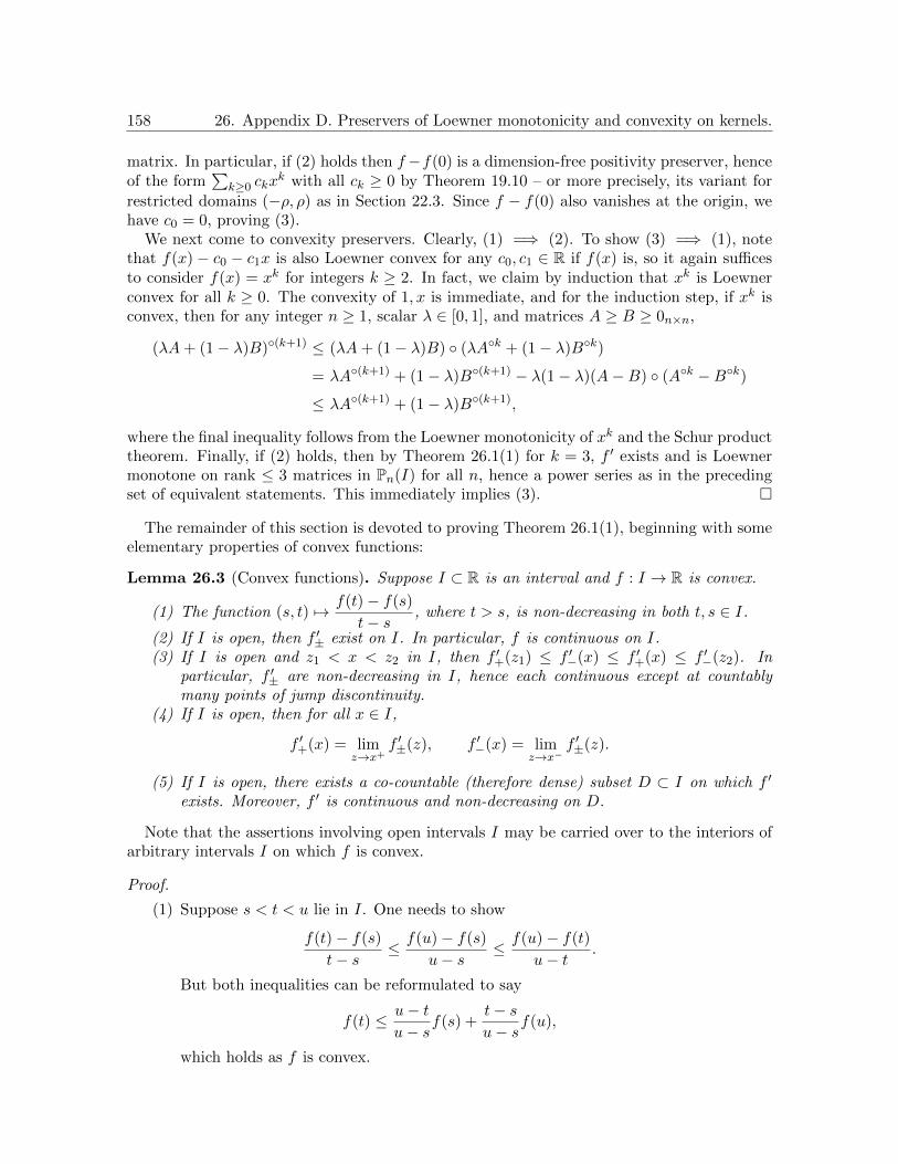
158 26. Appendix D. Preservers of Loewner monotonicity and convexity on kernels.

matrix. In particular, if (2) holds then f−f(0) is a dimension-free positivity preserver, henceof the form

∑k≥0 ckx

k with all ck ≥ 0 by Theorem 19.10 – or more precisely, its variant for

restricted domains (−ρ, ρ) as in Section 22.3. Since f − f(0) also vanishes at the origin, wehave c0 = 0, proving (3).

We next come to convexity preservers. Clearly, (1) =⇒ (2). To show (3) =⇒ (1), notethat f(x) − c0 − c1x is also Loewner convex for any c0, c1 ∈ R if f(x) is, so it again sufficesto consider f(x) = xk for integers k ≥ 2. In fact, we claim by induction that xk is Loewnerconvex for all k ≥ 0. The convexity of 1, x is immediate, and for the induction step, if xk isconvex, then for any integer n ≥ 1, scalar λ ∈ [0, 1], and matrices A ≥ B ≥ 0n×n,

(λA+ (1− λ)B)(k+1) ≤ (λA+ (1− λ)B) (λAk + (1− λ)Bk)

= λA(k+1) + (1− λ)B(k+1) − λ(1− λ)(A−B) (Ak −Bk)

≤ λA(k+1) + (1− λ)B(k+1),

where the final inequality follows from the Loewner monotonicity of xk and the Schur producttheorem. Finally, if (2) holds, then by Theorem 26.1(1) for k = 3, f ′ exists and is Loewnermonotone on rank ≤ 3 matrices in Pn(I) for all n, hence a power series as in the precedingset of equivalent statements. This immediately implies (3).

The remainder of this section is devoted to proving Theorem 26.1(1), beginning with someelementary properties of convex functions:

Lemma 26.3 (Convex functions). Suppose I ⊂ R is an interval and f : I → R is convex.

(1) The function (s, t) 7→ f(t)− f(s)

t− s, where t > s, is non-decreasing in both t, s ∈ I.

(2) If I is open, then f ′± exist on I. In particular, f is continuous on I.(3) If I is open and z1 < x < z2 in I, then f ′+(z1) ≤ f ′−(x) ≤ f ′+(x) ≤ f ′−(z2). In

particular, f ′± are non-decreasing in I, hence each continuous except at countablymany points of jump discontinuity.

(4) If I is open, then for all x ∈ I,

f ′+(x) = limz→x+

f ′±(z), f ′−(x) = limz→x−

f ′±(z).

(5) If I is open, there exists a co-countable (therefore dense) subset D ⊂ I on which f ′

exists. Moreover, f ′ is continuous and non-decreasing on D.

Note that the assertions involving open intervals I may be carried over to the interiors ofarbitrary intervals I on which f is convex.

Proof.

(1) Suppose s < t < u lie in I. One needs to show

f(t)− f(s)

t− s≤ f(u)− f(s)

u− s≤ f(u)− f(t)

u− t.

But both inequalities can be reformulated to say

f(t) ≤ u− tu− s

f(s) +t− su− s

f(u),

which holds as f is convex.

26. Appendix D. Preservers of Loewner monotonicity and convexity on kernels. 159

(2) Given t ∈ I, choose s < t < u in I, and note by the previous part that the ratio

f(x)− f(t)

x− t, x ∈ (t, u)

is non-increasing in x as x → t+ and bounded below byf(t)− f(s)

t− s. Thus, f ′+(t)

exists; a similar argument works to show f ′−(t) exists. In particular, the two limitslimx→t± f(x)− f(t) are both zero, proving f is continuous at t ∈ I.

(3) The second sentence follows from the first, which in turn follows from the first partby taking limits and is left to the reader.

(4) The preceding part implies f ′±(z) are non-decreasing as z → x− and non-increasingas z → x+, and shows “half” of the desired inequalities. We now show f ′+(x) ≥limz→x+ f

′+(z); the remaining similar inequalities are shown similarly, and again left

to the reader. Let y ∈ I, y > x; then the first part implies

f(y)− f(z)

y − z≥ f(y′)− f(z)

y′ − z, ∀x < z < y′ < y.

Taking y′ → z+, we have f ′+(z) ≤ f(y)−f(z)y−z . From above, f is continuous on I, so

f(y)− f(x)

y − x= lim

z→x+f(y)− f(z)

y − z≥ lim

z→x+f ′+(z).

Finally, taking y → x+ concludes the proof.(5) Let D ⊂ I be the subset where f ′ exists, which is if and only if f ′+ is continuous

(by the preceding part). In particular, D is co-countable from a previous part, andf ′ = f ′+ is continuous and non-decreasing on D by the same part.

The next preliminary result shows the continuity (respectively, differentiability) of mono-tone (respectively, convex) functions on 2× 2 matrices:

Proposition 26.4. Suppose 0 < ρ ≤ ∞, I = (−ρ, ρ), and g : I → R.

(1) If g[−] is monotone on P2(I), then g is continuous on I.(2) If g[−] is convex on P2(I), then g is differentiable on I.

Proof. We begin with the first assertion. It is easily verified that if g is monotone on P2(I),then g− g(0), when applied entrywise to P2(I), preserves positivity. Hence, by (the boundeddomain-variant of) Theorem 12.7, g is continuous on (0, ρ). Moreover, we may assume withoutloss of generality that g(0) = 0.

Now let 0 < a < ρ and 0 < ε < ρ− a; then the monotonicity of g implies(a+ ε aa a

)≥(ε 00 0

)≥ 02×2 =⇒

(g(a+ ε)− g(ε) g(a)

g(a) g(a)

)≥ 02×2.

Pre- and post-multiplying this last matrix by (1,−1) and (1,−1)T respectively, we haveg(a+ ε)− g(a) ≥ g(ε), and by the monotonicity of g (applied to ε12×2 ≥ ε′12×2 for 0 ≤ ε′ <ε < ρ), it follows that g is non-decreasing on [0, ρ). Now taking the limit as ε→ 0+, we have

0 = g(a+)− g(a) ≥ g(0+) ≥ 0,

where the first equality follows from the continuity of g. Hence, g is right continuous at 0.Next, for the continuity of g on (−ρ, 0), let

a ∈ (0, ρ), 0 < ε < min(a, ρ− a), A =

(1 −1−1 1

),

160 26. Appendix D. Preservers of Loewner monotonicity and convexity on kernels.

and deduce from the monotonicity of g:

(a+ ε)A ≥ aA ≥ (a− ε)A ≥ 0 =⇒ g[(a+ ε)A] ≥ g[aA] ≥ g[(a− ε)A].

The positivity of the difference matrices implies, upon taking determinants:

|g(a± ε)− g(a)| ≥ |g(−a∓ ε)− g(−a)|.Let ε→ 0+; then the continuity of g at a implies that at −a, as desired. A similar (one-sided)argument shows the left continuity of g at 0, via the step g(ε)− g(0) ≥ |g(−ε)− g(0)|.

Next, we come to the second assertion. If g is convex on P2(I), then restricting to thematrices a12×2 for a ∈ [0, ρ), it follows that g is convex on [0, ρ). Hence, g′+ exists on (0, ρ)by Lemma 26.3. Now suppose 0 < s < t < ρ and 0 < ε < ρ− t. Then by the convexity of g,(

t+ ε tt t

)≥(s+ ε ss s

)≥ 02×2 =⇒

(g(λ(t+ ε) + (1− λ)(s+ ε)) g(λt+ (1− λ)s)

g(λt+ (1− λ)s) g(λt+ (1− λ)s)

)≤ λ

(g(t+ ε) g(t)g(t) g(t)

)+ (1− λ)

(g(s+ ε) g(s)g(s) g(s)

),

for all λ ∈ [0, 1]. Write this inequality in the following form:

(α ββ β

)≥ 02×2. As above, pre-

and post-multiplying this last matrix by (1,−1) and (1,−1)T respectively yields

g(λt+ (1− λ)s+ ε)− g(λt+ (1− λ)s) ≤ λ(g(t+ ε)− g(t)) + (1− λ)(g(s+ ε)− g(s)).

Divide by ε and let ε → 0+; this shows g′+ is convex, hence continuous by Lemma 26.3, on(0, ρ).

Next, denote by g0, g1 the even and odd parts of g, respectively:

g0(t) :=1

2(g(t) + g(−t)), g1(t) :=

1

2(g(t)− g(−t)).

We claim that g0, g1 are convex on [0, ρ). Indeed, by the convexity of g we deduce for0 ≤ s ≤ t < ρ and λ ∈ [0, 1]:(

t −t−t t

)≥(s −s−s s

)≥ 0

=⇒(g(cλ) g(−cλ)g(−cλ) g(cλ)

)≤ λ

(g(t) g(−t)g(−t) g(t)

)+ (1− λ)

(g(s) g(−s)g(−s) g(s)

),

where cλ = λt + (1 − λ)s. Pre- and post-multiplying this last inequality by (1,±1) and(1,±1)T respectively, yields

g(λt+ (1− λ)s)± g(−(λt+ (1− λ)s)) ≤ λ(g(t)± g(−t)) + (1− λ)(g(s)± g(−s)).This yields: g0, g1 are convex on [0, ρ). Next, note that if 0 ≤ s < t < ρ, and 0 < ε ≤min(t− s, ρ− t), then

g(s+ ε)− g(s)

ε≤ g(t)− g(t− ε)

ε,

by Lemma 26.3(1). Taking ε→ 0+ shows that g′+(s) ≤ g′−(t) if 0 ≤ s < t < ρ and g is convex.Similarly, g′−(t) ≤ g′+(t); therefore,

g′+(s) ≤ g′−(t) = (g0)′−(t) + (g1)′−(t) ≤ (g0)′+(t) + (g1)′+(t) = g′+(t).

Since g′+ is continuous, letting s → t− shows (gj)′−(t) = (gj)

′+(t) for j = 0, 1. Thus, gj is

differentiable on (0, ρ). Since g0 is even and g1 is odd, they are also differentiable on (−ρ, 0).Hence, g0, g1, g are differentiable on I \ 0. Finally, let I ′ := (−2ρ/3, 2ρ/3) and define

26. Appendix D. Preservers of Loewner monotonicity and convexity on kernels. 161

h(x) := g(x + ρ/3). It is easy to check that h is convex on P2(I ′), so it is differentiable at−ρ/3 by the above analysis, and hence g is differentiable at 0, as desired.

With these preliminary results in hand, we now complete the remaining proof:

Proof of Theorem 26.1. We begin by showing the first assertion. First, suppose f is differen-tiable on I and f ′ is monotone on the rank ≤ k matrices in Pn(I). Also assume A ≥ B ≥ 0n×nare matrices of rank ≤ k. Now follow the proof of Proposition 15.9(3) to show that f [−] isLoewner convex on rank ≤ k matrices in Pn(I). Here we use the fact that since A ≥ B ≥ 0,we have the chain of Loewner inequalities

A ≥ λA+ (1− λ)B ≥ λA+B

2+ (1− λ)B ≥ B, (26.5)

and hence the ranks of all matrices here are at most rk(A) ≤ k.The converse is shown in two steps; in fact, we will also prove that f is continuously

differentiable on I. The first step is to show the result for n = k = 2. Note by Proposition 26.4that f is differentiable on I. Now say A ≥ B ≥ 02×2 with A 6= B in P2(I). Writing A =(a1 aa a2

)and B =

(b1 bb b2

), we have aj ≥ bj ≥ 0 for j = 1, 2 and (a−b)2 ≤ (a1−b1)(a2−b2).

Define δ ∈ [0, a1 − b1] and the matrix C2×2 via

(a− b)2 = (a1 − b1 − δ)(a2 − b2), C :=

(b1 + δ bb b2

)∈ P2(I).

Clearly, A ≥ C ≥ B, all matrices are in P2(I), and A − C,C − B have rank at most 1.Thus, we may assume without loss of generality that A − B has rank 1; write A − B =(

a√ab√

ab b

)∈ P2. First, if ab = 0, then f ′[A] − f ′[B] is essentially a scalar on the main

diagonal. Now since f is convex on [0, ρ) by considering a12×2 for a ∈ [0, ρ), we have f ′ isnon-decreasing on (0, ρ), and hence f ′[A] ≥ f ′[B].

The other case is a, b > 0. In this case A ≥ B ≥ 0 and A − B is rank-1 with no zeroentries. Now follow the proof of Proposition 15.9(3) to infer f ′[A] ≥ f ′[B]. Together, bothcases show that f ′ is monotone on P2(I), so f ′ is continuous on I by Proposition 26.4(1).

This shows the result for n = k = 2. Now suppose n > 2. First, f is convex on P2(I), sof ′ is monotone on P2(I) and hence continuous on I by the previous case. Second, to showthat f ′ is monotone as asserted, suppose A ≥ B ≥ 0n×n are matrices in Pn(I) of rank ≤ k.Now claim that there is a chain of Loewner matrix inequalities

A = An ≥ An−1 ≥ · · · ≥ A0 = B,

satisfying: (1) Aj ∈ Pn(I) for all 0 ≤ j ≤ n, and (2) Aj − Aj−1 has rank at most 1 for each1 ≤ j ≤ n. Note that such a chain of inequalities would already imply the reverse inclusionsfor the corresponding null spaces, so each Aj has rank at most k.

To show the claim, spectrally decompose A − B = UDUT , where U is orthogonal andD = diag(λ1, . . . , λn) with λj ≥ 0, and write

Aj := B + U diag(λ1, . . . , λj , 0, . . . , 0)UT , 0 ≤ j ≤ n.Note that Aj ≤ A, so the same applies to each of their corresponding (non-negative) diagonalentries. Thus, 0 ≤ (Aj)ll ≤ all for 1 ≤ l ≤ n. Thus, the diagonal entries of each Aj lie inI = (−ρ, ρ), hence so do the off-diagonal entries. This shows the claim.

Thus, to show f ′[A] = f ′[An] ≥ f ′[A0] = f ′[B], it suffices to assume, as in the previous caseof n = k = 2, that A−B has rank 1. First, if A−B has no zero entries, then f ′[A] ≥ f ′[B] by

162 26. Appendix D. Preservers of Loewner monotonicity and convexity on kernels.

Proposition 15.9(3). Otherwise, suppose A−B = uuT , with u ∈ Rn a non-zero vector having

zero entries. Without loss of generality, write u =

(v0

), with v ∈ Rl having no zero entries

for some 1 ≤ l ≤ n− 1. Accordingly, write A =

(A11 A12

A21 A22

), and similarly for B; it follows

that Aij = Bij for all (i, j) 6= (1, 1), and A11 = B11 + vvT . Now since f is Loewner convex on[B,A], it is so on [B11, A11], where all matrices are positive semidefinite and also have rank≤ k. Moreover, f ′ exists and is continuous on I from above. Again, by Proposition 15.9(3),it follows that f ′ is Loewner monotone on [B11, A11] (if k = 1 then this assertion is true byone-variable calculus). But then,

f ′[A]− f ′[B] =

(f ′[A11]− f ′[B11] 0

0 0

)≥ 0.

This proves the first assertion; we turn to the second. First, suppose A ≥ B ≥ 0n×n,and f ′ is Loewner positive on Pn(I). Then follow the proof of Proposition 15.9(2) to inferf [A] ≥ f [B]. Conversely, we prove the result under a stronger hypothesis: namely, f isdifferentiable. Now the proof of Proposition 15.9(2) again applies: given A ∈ Pn(I), we haveA+ ε1n×n ∈ Pn(I) for small ε > 0. By monotonicity, it follows that

1ε (f [A+ ε1n×n]− f [A]) ∈ Pn.

Taking ε→ 0+ proves f ′[A] ∈ Pn, as desired.

We now move to kernels.

Definition 26.6. Suppose X is a non-empty set, I ⊂ R a domain, and V is a set of (realsymmetric) positive semidefinite kernels on X ×X, with values in I.

(1) The Loewner order on kernels on X × X is: K L for K,L kernels on X × X, ifK − L is a positive semidefinite kernel. (Note, if X is finite, this specializes to theusual Loewner ordering on real |X| × |X| matrices.)

(2) A function F : I → R is Loewner monotone on V if F K F L whenever K L 0are kernels in V.

(3) A function F : I → R is Loewner convex on V (here I is assumed to be convex) ifwhenever K L 0 are kernels in V, we have

λF K + (1− λ)F L F (λK + (1− λ)L), ∀λ ∈ [0, 1].

The above results for matrices immediately yield the results for kernels:

Theorem 26.7. Suppose 0 < ρ ≤ ∞, I = (−ρ, ρ), and F : I → R, and X is an infinite set.The composition map F − is Loewner monotone (respectively, Loewner convex) on positivekernels on X ×X, if and only if F satisfies the respective equivalent conditions on matricesof all sizes, in Theorem 26.2.

Proof. First, if F is Loewner monotone or convex on kernels on X ×X, then by restrictingthe defining inequalities to kernels on Y × Y (padded by zeros) for finite sets Y ⊂ X, itfollows that F is, respectively, Loewner monotone or convex on Pn(I) for all n ≥ 1.

To show the converse, suppose first that F (y) =∑∞

k=0 ckyk on I, with c1, c2, · · · ≥ 0. To

show that F − is Loewner monotone on kernels on X × X, it suffices to do so on every“principal submatrix” of such kernels – i.e., for every finite indexing subset of X. But this isindeed true for F , by Theorem 26.2. A similar proof holds for Loewner convex maps.

27. Appendix E. Menger’s results and Euclidean distance geometry. 163

27. Appendix E. Menger’s results and Euclidean distance geometry.

We conclude this part of the text with a brief detour into the same area where we startedthis part of the text: metric geometry, specifically, that of Euclidean spaces Rn – and of theirclosure, Hilbert space `2. This is a beautiful area of mathematical discovery, which has fea-tured work by several prominent mathematicians, including Birkhoff, Cauchy, Cayley, Godel,Menger, Schoenberg, and von Neumann, among others. See [237] for a modern exposition ofsome of the gems of distance geometry (which begins, interestingly, with Heron’s formula forthe area of a triangle, from two millennia ago).

The main result of this section is a 1928 theorem of Menger:

Theorem 27.1 (Menger, [257]; see also [314]). A metric space (X, d) can be isometricallyembedded in Hilbert space `2 if and only if X is separable and every subset of X of size n+ 1can be isometrically embedded in Rn (equivalently, in `2) for n ≥ 2.

This result, together with Schoenberg’s theorems 16.10 and 16.17 on Hilbert space embed-dings of finite metric spaces X, immediately yields those theorems for all separable X:

Theorem 27.2 (Schoenberg). Suppose (X, d) is a separable metric space.

(1) X embeds isometrically into Hilbert space `2 if and only if for every integer n ≥ 2 and(n+1)-tuple of points Y := (x0, . . . , xn) in X, the “alternate Cayley–Menger matrix”CM ′(Y ) := (d(x0, xj)

2 + d(x0, xk)2 − d(xj , xk)

2)nj,k=1 is positive semidefinite.

(2) X embeds isometrically into Hilbert space `2 if and only if the Gaussian kernelexp(−σ(·)2) is a positive definite function on X for all σ > 0 (equivalently, for somesequence σm of positive numbers decreasing to 0+).

Here, we explore some simple, yet beautiful observations in Euclidean distance geometry,which help prove Theorem 27.1, and also provide connections to Cayley–Menger matrices [78,258] and to n-point homogeneous spaces (see Remark 16.22). We begin with the latter.

27.1. n-point homogeneity of Euclidean and Hilbert spaces. As early as 1944, in hisinfluential work [50] Birkhoff defines a metric space (X, d) to be n-point homogeneous if giventwo equinumerous subsets of X of size at most n, an isometry between them extends to aself-isometry of X. The heart of the present proof of Theorem 27.1 is to show that Euclideanspace Rk is n-point homogeneous for all k, n ≥ 1:

Theorem 27.3. Fix an integer k ≥ 1.

(1) The Euclidean space Rk with the Euclidean metric is n-point homogeneous for all n.More strongly: any isometry between two subsets M,N ⊂ Rk is, up to a translation,the restriction of an orthogonal linear transformation of Rk.

(2) Hilbert space `2 is n-point homogeneous for all n.

The first step in proving Theorem 27.3 is the following observation about Gram matrices:

Lemma 27.4. Given vectors y0, . . . , yn ∈ `2 for some n ≥ 0, the Gram matrix (〈yj , yk〉)nj,k=0

is invertible if and only if the yj are linearly independent.

Proof. We prove the contrapositive. If∑n

k=0 ckyk = 0 is a nontrivial linear combination, thenapplying 〈yj ,−〉 for all j yields Gram((yk)k)c = 0, where c = (c0, . . . , cn)T 6= 0. Conversely,if Gram((yk)k)c = 0 and c 6= 0, then

0 = cT Gram((yk)k)c =

∥∥∥∥∥n∑k=0

ckyk

∥∥∥∥∥2

,

164 27. Appendix E. Menger’s results and Euclidean distance geometry.

so that some nontrivial linear combination of the yk vanishes, as desired.

This simple lemma leads to striking consequences. We will presently mention two, the firstof which involves a classical concept (which already featured in Theorem 16.10):

Definition 27.5. Given a metric space X = (x0, x1, . . . , xn, d), write djk := d(xj , xk) for0 ≤ j, k ≤ n. The associated Cayley–Menger matrix is

CM(X)(n+2)×(n+2) :=

0 d201 d2

02 · · · d20n 1

d210 0 d2

12 · · · d21n 1

d220 d2

21 0 · · · d22n 1

......

.... . .

......

d2n0 d2

n1 d2n2 · · · 0 1

1 1 1 · · · 1 0

, (27.6)

Similarly, the “alternate form” of the Cayley–Menger matrix here is

CM ′(X)n×n :=

2d2

01 d201 + d2

02 − d212 · · · d2

01 + d20n − d2

1n

d201 + d2

02 − d212 2d2

02 · · · d201 + d2

0n − d21n

......

. . ....

d201 + d2

0n − d21n d2

02 + d20n − d2

2n · · · 2d20n

(27.7)

Recall that the positive semidefiniteness of the second matrix features in Schoenberg’srecasting of Menger and Frechet’s results on Hilbert space embeddings of finite metric spaces.We now write down a preliminary observation that relates the two determinants above:

Lemma 27.8. For all finite metric spaces X with at least two points,

detCM(X) = (−1)|X| detCM ′(X). (27.9)

Proof. Starting with the matrix CM(X), perform elementary row and column operations,leaving the determinant unchanged. First, subtract the first row from all non-extremal rows.Then subtract the first and last columns each from the non-extremal columns. This yields 0 0Tn 1

0n −CM ′(X) 0n1 0Tn 0

,

a bordered matrix with determinant (−1)n+1 detCM ′(X), as desired.

We can now state and prove the two consequences of Lemma 27.4 promised above. Thefirst of these is a well-known result, proved in 1841 by Cayley during his undergraduate days[78]. The second is the underlying principle behind the Global Positioning System, or GPS –trilateration (also referred to more colloquially as “triangulation”): every point in the plane(or on the surface of a sphere “like” the Earth) is uniquely determined by intersecting threecircles that denote distances from three non-collinear points (or four spheres centered at fournon-coplanar points).

Proposition 27.10.

(1) (Cayley, [78]). Suppose an isometry Ψ sends a finite metric space (X = x0, . . . , xn, d)into Hilbert space `2. Then the vectors Ψ(x0), . . . ,Ψ(xn) are affine linearly dependent(i.e., lie on an (n− 1)-dimensional subspace) in `2, if and only if the Cayley–Mengerdeterminant of X vanishes.

(2) Fix vectors y0 = 0, y1, . . . , yn ∈ `2. Given any y ∈ `2, the following are equivalent:

27. Appendix E. Menger’s results and Euclidean distance geometry. 165

(a) y is (uniquely) determined by the tuple of Euclidean distances (‖y‖, ‖y−y1‖, . . . , ‖y−yn‖) ∈ Rn+1.

(b) y is in the span of y1, . . . , yn.

Proof.

(1) Denote yj := Ψ(xj) for 0 ≤ j ≤ n. Now compute, as in Equation (16.12) in the proofof Theorem 16.10:

d(y0, yj)2 + d(y0, yk)

2 − d(yj , yk)2 = 〈y0 − yj , y0 − yk〉,

so that CM ′(X) = Gram((y0 − yj)nj=1). Now CM(X) is singular if and only if so is

CM ′(X). From above and by Lemma 27.4, this happens if and only if the vectorsy0 − yj , 1 ≤ j ≤ n are linearly dependent. This completes the proof.

(2) For this part, let V ⊂ `2 denote the span of the yj . First, suppose y 6∈ V . Writey = yV ⊕ yV ⊥ as the orthogonal decomposition of y. One verifies that for any unitvector v ∈ V ⊥ (for instance, v = ±yV ⊥/‖yV ⊥‖), both y as well as the vector

yV ⊕ ‖yV ⊥‖v

have the same distances from every vector in V – in particular, from each of 0, y1, . . . , yn.This shows (the contrapositive of) one implication.

Conversely, suppose y ∈ V . We show that y is uniquely determined by the distancesto the yj and to 0 – in fact, it suffices to consider the distances to a basis of V .Thus, suppose without loss of generality that the yj are linearly independent. Lety :=

∑nj=1 cjyj , and let d0 := ‖y‖, dj := ‖y − yj‖. We show that the dj uniquely

determine the cj , and hence y. Indeed, a straightforward computation yields

d20 − d2

j =

∥∥∥∥∥n∑k=1

ckyk

∥∥∥∥∥2

−

∥∥∥∥∥n∑k=1

ckyk − yj

∥∥∥∥∥2

= −‖yj‖2 + 2n∑k=1

ck〈yj , yk〉, 1 ≤ j ≤ n.

Rewriting this system of linear equations (in c = (c1, . . . , cn)) yields

Gram((yj)j)c =1

2(‖y‖2 + ‖yj‖2 − ‖y − yj‖2)nj=1. (27.11)

Hence, c is unique, by Lemma 27.4.

Equipped with these preliminaries, we are now ready to proceed toward proving Menger’sresult. We first show:

Proof of Theorem 27.3.

(1) First suppose that both M,N contain the origin, and Ψ : M → N sends 0 to itself.This is not really a constraint: if here we can show that Ψ = T |M for some orthogonalmatrix T ∈ Ok(R), then for a general isometry Ψ and an arbitrary (base)point m ∈M , the isometry

Φ : M −m → Ψ(M)−Ψ(m), v 7→ Ψ(m + v)−Ψ(m)

sends 0 to 0, hence equals the restriction to M of some T ∈ Ok(R). Thus,

Ψ(m) = T (m) + (Ψ(m)− T (m)), ∀m ∈M.

Therefore, we may assume without loss of generality that m := 0 ∈ M ∩ N andΨ(0) = 0. In this case, we need to show that Ψ is the restriction to M of an orthogonalmatrix.

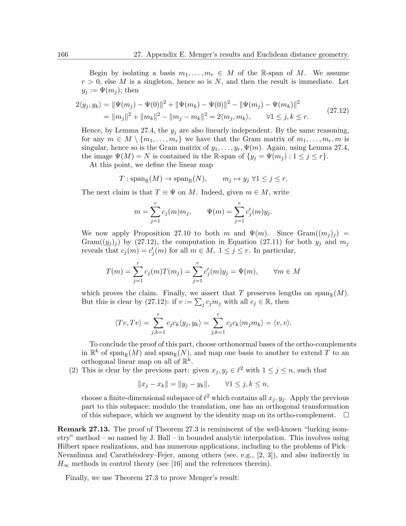
166 27. Appendix E. Menger’s results and Euclidean distance geometry.

Begin by isolating a basis m1, . . . ,mr ∈ M of the R-span of M . We assumer > 0, else M is a singleton, hence so is N , and then the result is immediate. Letyj := Ψ(mj); then

2〈yj , yk〉 = ‖Ψ(mj)−Ψ(0)‖2 + ‖Ψ(mk)−Ψ(0)‖2 − ‖Ψ(mj)−Ψ(mk)‖2

= ‖mj‖2 + ‖mk‖2 − ‖mj −mk‖2 = 2〈mj ,mk〉, ∀1 ≤ j, k ≤ r.(27.12)

Hence, by Lemma 27.4, the yj are also linearly independent. By the same reasoning,for any m ∈ M \ m1, . . . ,mr we have that the Gram matrix of m1, . . . ,mr,m issingular, hence so is the Gram matrix of y1, . . . , yr,Ψ(m). Again, using Lemma 27.4,the image Ψ(M) = N is contained in the R-span of yj = Ψ(mj) : 1 ≤ j ≤ r.

At this point, we define the linear map

T : spanR(M)→ spanR(N), mj 7→ yj ∀1 ≤ j ≤ r.

The next claim is that T ≡ Ψ on M . Indeed, given m ∈M , write

m =r∑j=1

cj(m)mj , Ψ(m) =r∑j=1

c′j(m)yj .

We now apply Proposition 27.10 to both m and Ψ(m). Since Gram((mj)j) =Gram((yj)j) by (27.12), the computation in Equation (27.11) for both yj and mj

reveals that cj(m) = c′j(m) for all m ∈M, 1 ≤ j ≤ r. In particular,

T (m) =r∑j=1

cj(m)T (mj) =r∑j=1

c′j(m)yj = Ψ(m), ∀m ∈M

which proves the claim. Finally, we assert that T preserves lengths on spanR(M).But this is clear by (27.12): if v :=

∑j cjmj with all cj ∈ R, then

〈Tv, Tv〉 =r∑

j,k=1

cjck〈yj , yk〉 =r∑

j,k=1

cjck〈mjmk〉 = 〈v, v〉.

To conclude the proof of this part, choose orthonormal bases of the ortho-complementsin Rk of spanR(M) and spanR(N), and map one basis to another to extend T to anorthogonal linear map on all of Rk.

(2) This is clear by the previous part: given xj , yj ∈ `2 with 1 ≤ j ≤ n, such that

‖xj − xk‖ = ‖yj − yk‖, ∀1 ≤ j, k ≤ n,

choose a finite-dimensional subspace of `2 which contains all xj , yj . Apply the previouspart to this subspace; modulo the translation, one has an orthogonal transformationof this subspace, which we augment by the identity map on its ortho-complement.

Remark 27.13. The proof of Theorem 27.3 is reminiscent of the well-known “lurking isom-etry” method – so named by J. Ball – in bounded analytic interpolation. This involves usingHilbert space realizations, and has numerous applications, including to the problems of Pick–Nevanlinna and Caratheodory–Fejer, among others (see, e.g., [2, 3]), and also indirectly inH∞ methods in control theory (see [16] and the references therein).

Finally, we use Theorem 27.3 to prove Menger’s result:

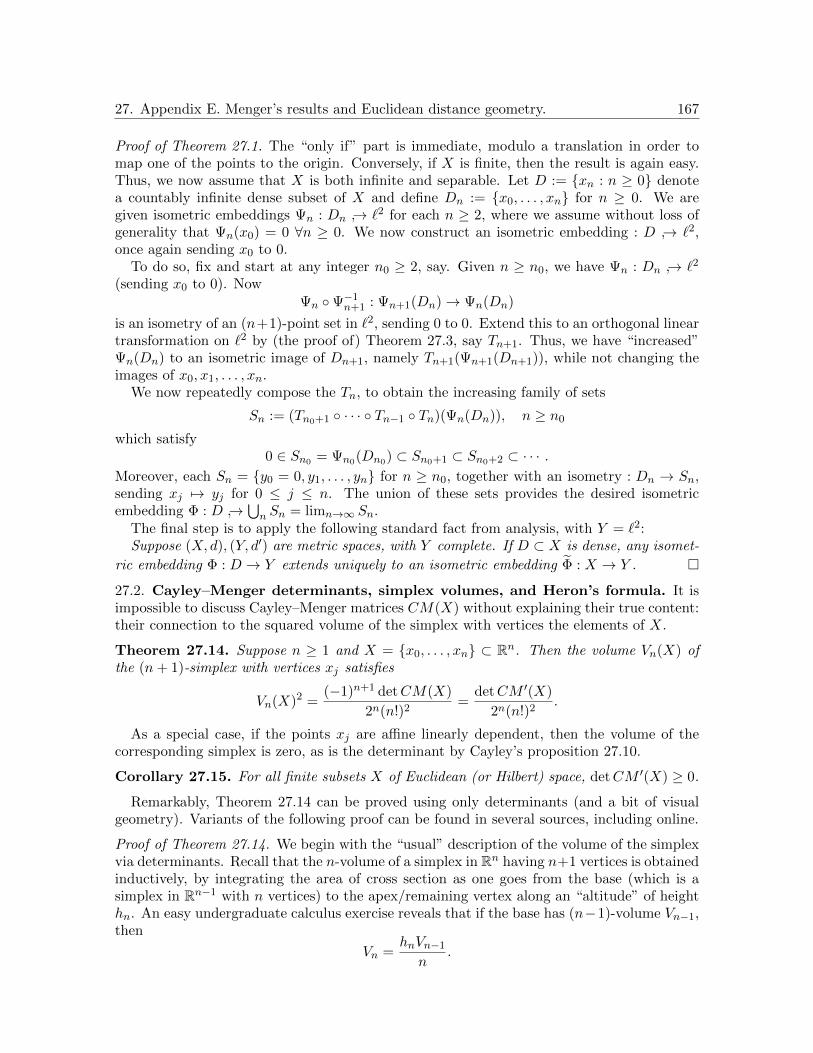
27. Appendix E. Menger’s results and Euclidean distance geometry. 167

Proof of Theorem 27.1. The “only if” part is immediate, modulo a translation in order tomap one of the points to the origin. Conversely, if X is finite, then the result is again easy.Thus, we now assume that X is both infinite and separable. Let D := xn : n ≥ 0 denotea countably infinite dense subset of X and define Dn := x0, . . . , xn for n ≥ 0. We aregiven isometric embeddings Ψn : Dn → `2 for each n ≥ 2, where we assume without loss ofgenerality that Ψn(x0) = 0 ∀n ≥ 0. We now construct an isometric embedding : D → `2,once again sending x0 to 0.

To do so, fix and start at any integer n0 ≥ 2, say. Given n ≥ n0, we have Ψn : Dn → `2

(sending x0 to 0). NowΨn Ψ−1

n+1 : Ψn+1(Dn)→ Ψn(Dn)

is an isometry of an (n+1)-point set in `2, sending 0 to 0. Extend this to an orthogonal lineartransformation on `2 by (the proof of) Theorem 27.3, say Tn+1. Thus, we have “increased”Ψn(Dn) to an isometric image of Dn+1, namely Tn+1(Ψn+1(Dn+1)), while not changing theimages of x0, x1, . . . , xn.

We now repeatedly compose the Tn, to obtain the increasing family of sets

Sn := (Tn0+1 · · · Tn−1 Tn)(Ψn(Dn)), n ≥ n0

which satisfy0 ∈ Sn0 = Ψn0(Dn0) ⊂ Sn0+1 ⊂ Sn0+2 ⊂ · · · .

Moreover, each Sn = y0 = 0, y1, . . . , yn for n ≥ n0, together with an isometry : Dn → Sn,sending xj 7→ yj for 0 ≤ j ≤ n. The union of these sets provides the desired isometricembedding Φ : D →

⋃n Sn = limn→∞ Sn.

The final step is to apply the following standard fact from analysis, with Y = `2:Suppose (X, d), (Y, d′) are metric spaces, with Y complete. If D ⊂ X is dense, any isomet-

ric embedding Φ : D → Y extends uniquely to an isometric embedding Φ : X → Y .

27.2. Cayley–Menger determinants, simplex volumes, and Heron’s formula. It isimpossible to discuss Cayley–Menger matrices CM(X) without explaining their true content:their connection to the squared volume of the simplex with vertices the elements of X.

Theorem 27.14. Suppose n ≥ 1 and X = x0, . . . , xn ⊂ Rn. Then the volume Vn(X) ofthe (n+ 1)-simplex with vertices xj satisfies

Vn(X)2 =(−1)n+1 detCM(X)

2n(n!)2=

detCM ′(X)

2n(n!)2.

As a special case, if the points xj are affine linearly dependent, then the volume of thecorresponding simplex is zero, as is the determinant by Cayley’s proposition 27.10.

Corollary 27.15. For all finite subsets X of Euclidean (or Hilbert) space, detCM ′(X) ≥ 0.

Remarkably, Theorem 27.14 can be proved using only determinants (and a bit of visualgeometry). Variants of the following proof can be found in several sources, including online.

Proof of Theorem 27.14. We begin with the “usual” description of the volume of the simplexvia determinants. Recall that the n-volume of a simplex in Rn having n+1 vertices is obtainedinductively, by integrating the area of cross section as one goes from the base (which is asimplex in Rn−1 with n vertices) to the apex/remaining vertex along an “altitude” of heighthn. An easy undergraduate calculus exercise reveals that if the base has (n−1)-volume Vn−1,then

Vn =hnVn−1

n.

168 27. Appendix E. Menger’s results and Euclidean distance geometry.

One can now proceed inductively. Thus, let h1 denote the length ‖x0 − x1‖, let h2 denotethe “height” of x2 “above” the segment joining x0, x1 (so it can be written as the norm of asuitable orthogonal complement), and so on. Then,

Vn(X) =1

n!hnhn−1 · · ·h1.

We now show that this product expression equals (up to sign) a determinant. Write

xj := (x(1)j , . . . , x

(n)j )T ∈ Rn, 0 ≤ j ≤ n

and claim that the volume equals, up to a sign,

Vn(X) = ± 1

n!det(A), where A := (x

(k)j − x

(k)0 )nj,k=1. (27.16)

To show the claim, note that working with A essentially amounts to assuming x0 = 0. Choos-ing a suitable orthonormal basis (i.e., by applying a suitable orthogonal transformation), wemay further assume that x1, . . . , xn−1 ∈ Rn−1 – thus, the final column of A has all entries zeroexcept at most the (n, n) entry. Now the final row of A, which denotes the vector xn − x0,may be replaced by its orthogonal complement to the span of xj − x0 : j < n withoutchanging the determinant, and so we obtain (up to a sign) the height hn – and in the nthcoordinate since xj − x0 ∈ Rn−1 for j < n. This scalar can be taken out of the determinantand we are now left with the determinant of an (n− 1)× (n− 1) matrix.

Applying the same arguments for xj − x0 with j ≤ n− 2 now, we obtain hn−1, and so on.Proceeding by downward induction (and taking the absolute value), we obtain (27.16).

The remainder of the proof consists of matrix manipulations. The next variant is to observethat (up to a sign), the volume of the simplex on X equals

1

n!det(x

(k)j − x

(k)0 )nj,k=1 =

1

n!detA =

1

n!det

(1 0Tn1n A

).

Add x(k)0 times the first column to the kth column in the final matrix to get 1

n!

1 xT0...

...1 xTn

.

Post-multiplying this matrix by its transpose gives,

Vn(X)2 =1

(n!)2det(1 + xTj xk)

nj,k=0 =

1

(n!)2det

(1 1Tn+1

0n+1 (1 + xTj xk)nj,k=0

).

Subtracting the first row from every other row gives,

Vn(X)2 =1

(n!)2det

(1 1Tn+1

−1n+1 (〈xj , xk〉)nj,k=0

).

One can expand this determinant along the first row. Now the cofactor of the (1, 1) entry iszero, since it is a (n + 1) × (n + 1) Gram matrix of vectors in Rn (so has rank at most n).Thus, we may replace the (1, 1)-entry in the above matrix by 0 and leave the determinantunchanged. First do this, then take out a factor of −1 from the first column and of −1/2from all other columns, and finally, a factor of −2 from the first row, to obtain

Vn(X)2 =(−1)n+1

2n(n!)2det

(0 1Tn+1

1n+1 (−2〈xj , xk〉)nj,k=0

).

27. Appendix E. Menger’s results and Euclidean distance geometry. 169

Finally, add 〈xj , xj〉 times the initial row to the row containing −2〈xj , xk〉 – for each 0 ≤j ≤ n. Also perform the analogous column operations. This yields precisely the Cayley–Menger matrix CM(X), with the final row and column moved to the initial row and column,respectively. As these permutations leave the determinant unchanged, it follows that

Vn(X)2 =(−1)n+1

2n(n!)2detCM(X).

The proof is complete by Equation (27.9).

As a special case, this result leads to a well-known formula from two thousand years ago:

Corollary 27.17 (Heron’s formula). A (Euclidean) triangle with edge lengths a, b, c and

semi-perimeter s = 12(a+ b+ c) has area

√s(s− a)(s− b)(s− c).

Proof. Explicitly expand the determinant in Theorem 27.14 for n = 2, to obtain:

V 22 =

−1

16det

0 a2 b2 1a2 0 c2 1b2 c2 0 11 1 1 0

=−1

16(−(a+ b+ c)(a+ b− c)(b+ c− a)(c+ a− b)) ,

and this is precisely s(s− a)(s− b)(s− c).

27.3. Complements: completely monotone functions and distance transforms. Inparallel to the use of absolutely monotone functions earlier in this text – to characterizepositivity preservers of kernels on infinite domains (or all finite domains) – we present herea related result by Ressel that features completely monotone functions. We then provide asampling of early results in metric geometry, again by Schoenberg, that feature such functions.

Definition 27.18. A function f : (0,∞) → R is completely monotone if f is smooth and

(−1)kf (k) is non-negative on (0,∞) for all k ≥ 0. A continuous function f : [0,∞) → R iscompletely monotone if the restriction of f to (0,∞) is completely monotone.

For instance, x−α for α ≤ 0 is completely monotone on (0,∞).We start with two results which are easily reformulated in the language of kernels:

(1) In his 1974 paper [296], Ressel characterized the functions that are positive definite ina different sense: given an abelian semigroup (S,+), a function f : S → R is said to bepositive semidefinite if f is bounded and for any finite set of elements s1, . . . , sn ∈ S,the matrix (f(sj + sk))

nj,k=1 is positive semidefinite. Ressel then showed for all p ≥ 1

that the continuous and positive semidefinite functions on the semigroup [0,∞)p areprecisely Laplace transforms of finite non-negative Borel measures on [0,∞)p. Inparticular, for p = 1, this is further equivalent – by a result attributed to Bernstein,Hausdorff, and Widder – to f being completely monotone on [0,∞).

(2) A related result to this was shown by Schoenberg [315] in Ann. of Math. (1938). Itsays that a continuous function f : [0,∞) → R satisfies the property that for allintegers m,n ≥ 1 and vectors x1, . . . , xm ∈ Rn, the matrix (f(‖xj − xk‖2))mj,k=1 ispositive semidefinite, if and only if f is completely monotone – i.e., as mentioned inthe previous part, there exists a finite non-negative measure µ on [0,∞), such that

f(x) =

∫ ∞0

exp(−xt) dµ(t), ∀x ≥ 0.

Completely monotone functions also feature in the study of metric “endomorphisms” ofEuclidean spaces. For instance, Schoenberg proved (in the aforementioned 1938 paper):

170 27. Appendix E. Menger’s results and Euclidean distance geometry.

Theorem 27.19. Given a continuous map f : [0,∞)→ [0,∞), the following are equivalent:

(1) For all integers m,n ≥ 1 and vectors x1, . . . , xm ∈ Rn, the matrix (f(‖xj −xk‖))mj,k=1

is Euclidean – i.e., xj with the metric f ‖ · ‖ isometrically embeds into `2.

(2) We have f(0) = 0 and the function ddx(f(

√x)2) is completely monotone on (0,∞).

This result and paper are part of Schoenberg’s program [312, 315, 316, 317, 354] to under-stand the transforms taking distance matrices from Euclidean space En of one dimension n,isometrically to those from another, say Em. Schoenberg denoted this problem by En;Em,with 1 ≤ m,n ≤ ∞, where E∞ ∼= `2 is Hilbert space. Schoenberg showed:

(1) If n > m, then En;Em is given by only the trivial function f(t) ≡ 0. Indeed, firstobserve by induction on n that the only Euclidean configuration of n+ 1 points thatare equidistant from one another is an “equilateral” (n+ 1)-simplex ∆ in Rn (or En),hence in any higher-dimensional Euclidean space – and this cannot exist in Rn−1,hence not in Rm for m < n. If now f(x0) 6= 0 for some x0 > 0, then applying f to thedistance matrix between vertices of the rescaled simplex x0∆ ⊂ Rn, produces n + 1equidistant points in Rm, which is not possible if 1 ≤ m < n.

(2) If 2 ≤ n ≤ m < ∞, then En;Em consists only of the homotheties f(x) = cx forsome c ≥ 0. (With von Neumann in 1941 [354], Schoenberg then extended this toanswer the question for n = 1 ≤ m ≤ ∞.) Schoenberg also provided answers forE2;E∞.

(3) The solution to the problem E∞;E∞ is precisely the content of Theorem 27.19.

As a special case of Theorem 27.19, all powers δ ∈ (0, 1) of the Euclidean metric embed intoEuclidean space. We provide an alternate proof using the above results on metric geometry.

Corollary 27.20 (Schoenberg, [314, 315]). Hilbert space `2, with the metric ‖x−y‖δ, embedsisometrically in “usual” `2 for any δ ∈ (0, 1).

This was shown in 1936 by Blumenthal in Duke Math. J. [52] for four-point subsets of `2

and δ ∈ (0, 1/2). Schoenberg extended this to all finite sets.

Proof. As observed by Schoenberg in [314], it suffices to show the result for (n+ 1)-elementsubsets x0, . . . , xn ⊂ `2, by Menger’s theorem 27.1. Now note that for c > 0, the functiong(u) := (1−e−cu)/u is bounded and continuous on (0, 1], hence admits a continuous extensionto [0, 1]. Since u−δ is integrable in (0, 1], so is the product

ϕ : (0, 1]→ R, u 7→ u−1−δ(1− e−cu).

Clearly, ϕ : [1,∞)→ R is also integrable, being continuous, non-negative, and bounded aboveby u−1−δ. By changing variables, we obtain a normalization constant cδ > 0, such that

t2δ = cδ

∫ ∞0

(1− e−λ2t2)λ−1−2δ dλ, ∀t > 0.

Set t := ‖xj − xk‖, and let u = (u0, . . . , un)T ∈ Rn+1 with∑

j uj = 0. Then,

n∑j,k=0

ujuk‖xj − xk‖2δ = cδ

∫ ∞0

n∑j,k=0

ujuk(1− e−λ2‖xj−xk‖2)

λ−1−2δ dλ.

But the double-sum inside the integrand equals −∑

j,k ujuke−λ2‖xj−xk‖2 , and this is non-

positive by Theorem 16.17. It follows that the matrix (−(‖xj − xk‖δ)2)nj,k=0 is conditionallypositive semidefinite, and so we are done by Theorem 16.10 and Lemma 16.13.

Part 3: Bibliographic notes and references 171

Bibliographic notes and references

Lemma 16.1 is taken from the well-known monograph [288] by Polya and Szego. Theo-rems 16.2, 16.3, 16.4, 16.5, 16.6, and 16.7, classifying the dimension-free entrywise positivitypreservers on various domains, are due to Schoenberg [317], Rudin [305], Vasudeva [352],Herz [170], and Christensen and Ressel [82, 83], respectively. The theorems of Schoenbergand Rudin and Vasudeva were recently shown by Belton–Guillot–Khare–Putinar in [31] usingsignificantly smaller test sets than all positive semidefinite matrices of all sizes; proving theseresults is the main focus of this part. These results turn out to be further useful in Part 4,in fully classifying the total positivity preservers on bi-infinite domains.

Loewner’s theorem 16.8 on operator/matrix monotone functions is from [240]; see alsoDonoghue’s book [103], as well as the recent monograph by Simon [337] that contains adozen different proofs.

The results in distance geometry are but a sampling from the numerous works of Schoen-berg. Theorem 16.10, relating Euclidean embedding of a metric and the conditional neg-ativity of the corresponding squared-distance matrix, is from [312], following then-recentworks by Menger [257, 258, 259] and Frechet [131]. Schoenberg’s theorem 16.17 (respectively,Proposition 16.19), characterizing Hilbert space (respectively, the Hilbert sphere) in terms ofpositive definiteness of the Gaussian family (respectively, the cosine), is from [316] (respec-tively, from [312]). We point out that Schoenberg proved these results more generally forseparable (not just finite) metric spaces, as discussed in Section 27. See also Schoenberg’spaper [315] and another with von Neumann [354] (and its related work [223] by Kolmogorov).For the works of Bochner in this context, we restrict ourselves to mentioning [56, 57]. Theo-rems 16.20 and 16.24 by Schoenberg on positive definite functions on spheres are from [317].Also, see the survey [345] of positive definite functions by James Drewry Stewart (who isperhaps somewhat better known for his series of calculus textbooks).

While Schoenberg’s motivations in arriving at his theorem lay in metric geometry, asdescribed above, Rudin’s motivations were from Fourier analysis. More precisely, Rudin wasstudying functions operating on spaces of Fourier transforms of L1 functions on groups G,or of measures on G. Here, G is a locally compact abelian group equipped with its Haarmeasure; Rudin worked with the torus G = T, while Kahane and Katznelson worked withits dual group Z. These authors together with Helson proved [164] a remarkable result ina converse direction to Wiener–Levy theory, in Acta Math. 1959. That same year, Rudinshowed Schoenberg’s theorem without the continuity hypothesis, i.e., Theorem 16.3. Formore details on this part, on the metric geometric motivations of Schoenberg, and othertopics, the reader is referred to the detailed recent twin surveys of Belton–Guillot–Khare–Putinar [27, 28].

The Horn–Loewner Theorem 17.1 (in a special case) originally appeared in Horn’s pa-per [182], where he attributes it to Loewner. The theorem has since been extended by theauthor (jointly) in various ways; see, e.g., [31, 155]; a common, overarching generalization ofthese and other variants has been achieved in [214]. Horn–Loewner’s determinant calculationin Proposition 17.5 was also extended to Proposition 17.8 by Khare [214]. The second, directproof of Theorem 17.1 is essentially due to Vasudeva [352].

Mollifiers were introduced by Friedrichs [132], following the famous paper of Sobolev [342],and their basic properties can be found in standard textbooks in analysis, as can Cauchy’smean value theorem for divided differences. The remainder of the proof of the strongerHorn–Loewner theorem is from [182], and the Boas–Widder theorem 18.10(2) is from [55].

172 Part 3: Bibliographic notes and references

Bernstein’s theorem 19.3 is from his well-known memoir on absolutely monotone func-tions [44]; see also Widder’s textbook [369]. Boas’ theorem 19.9 on the analyticity of smoothfunctions with SSR (strictly sign regular) derivatives is from [54]. Hamburger’s theorem 19.14is a folklore result, found in standard reference books – see, e.g., [8, 309, 334]. The remainderof Section 19 is from Belton–Guillot–Khare–Putinar [31]. Section 20 is taken from the samepaper, with the exception of Theorem 20.11 which is new, as are “Proofs 1 and 2” of theexistence of a positivity certificate/limiting sum-of-squares representation for (1± t)(1− t2)n.The former proof cites a result by Berg–Christensen–Ressel [39], and the latter, direct proof,is new.

Sections 21 and 22 are again from [31], save for the standard Identity Theorem 21.4, andProposition 21.2 on the closure of real analytic functions under composition; these can befound in, e.g., [227]. The complex analysis basics, including Montel and Morera’s theorems,can be found in standard textbooks; we cite [88]. The multivariate Schoenberg–Rudin the-orem was proved by FitzGerald, Micchelli, and Pinkus in [124], and subsequently, undersignificantly weaker hypotheses in [31].

Appendix A on the Boas–Widder theorem is from [55] except for the initial observations.Boas and Widder mention Popoviciu [289] had proved the same result previously, using un-equally spaced difference operators. The very last “calculus” Proposition 23.12 can be foundin standard textbooks. Appendix B, classifying the dimension-free preservers of positivitywhen not acting on diagonal blocks, is from the recent work of Vishwakarma [353], with theexception of the textbook Proposition 24.4, and Theorem 24.1 by Guillot–Rajaratnam [157].

Theorems 26.1 and 26.2 in Appendix D, understanding and relating the Loewner positive,monotone, and convex maps, were originally proved without rank constraints on the test sets,by Hiai in [171]. Lemma 26.3 is partly taken from [171] and partly from Rockafellar’s book– see [301, Theorems 24.1 and 25.3]. The remainder of Section 26 (i.e., Appendix D), as wellas Section 25 (i.e., Appendix C), are taken from Belton–Guillot–Khare–Putinar [32].

Theorem 27.1 is due to Menger [257]. Theorem 27.2 comes from various works of Schoen-berg on metric geometry (cited on the preceding page). Theorem 27.3 was already knownto experts at the time; we cite here Birkhoff’s famous paper [50]. The first part of Proposi-tion 27.10 was shown by Cayley [78], and features Cayley–Menger determinants. The proofof Theorem 27.14 can be found in numerous sources, including online. The results in Sec-tion 27.3 are taken from the sources mentioned in it (e.g., the proof of Corollary 27.20).

Part 4:

Polya frequency functionsand sequences

28. Totally non-negative functions of finite order. 175

Part 4: Polya frequency functions and sequences

28. Totally non-negative functions of finite order.

In this part and the next, we approach the preserver problem in the above settings througha more classical viewpoint: that of spaces of kernels and their endomorphisms. The materialin this part of the text is drawn primarily from the work of Schoenberg and his coauthors(as well as its account in Karlin’s monograph), and a few recent preprints, all from 2020.

We begin by describing this part of the text and the next. We are interested in character-izing the preservers of totally non-negative or totally positive kernels, on X ×Y for arbitrarytotally ordered sets X,Y . The case of X,Y finite was studied in Part 2, and if |X|, |Y | ≥ 2,the only such functions – up to rescaling – are powers. Next, if exactly one of X,Y is finite, aworkaround can be achieved by using a generalization of Whitney’s density theorem 6.7; weshow this in Section 40. The difficulty lies in the remaining case: classifying the total posi-tivity preservers for kernels on X × Y when both X,Y are infinite. In this case, the familiesof kernels we have encountered so far, do not suffice to yield a complete classification.

Thus, we begin by relaxing our goal, to classifying such preservers for structured kernels, onspecific domains. Our first goal is to study the inner transforms of TN/TP Toeplitz kernelson R × R. This is not an arbitrary choice: indeed, such kernels have long been studied inthe analysis literature, under the name of Polya frequency functions, and so it is natural tostudy this test set – as well as the related Polya frequency sequences – and to understand theendomorphisms of these classes. This understanding is achieved in the next part of the text.

The class of Polya frequency functions is fundamental to time-frequency analysis and tointerpolation theory, the latter via splines (a subject which begins with many papers bySchoenberg and his coauthors). Polya frequency functions possess beautiful properties thatwere established by Schoenberg and others in the twentieth century, and that allow us toexploit tools from harmonic analysis to try and classify their preservers. Looking ahead (andusing these tools), we will find that Toeplitz TN kernels turn out to be quite rigid, andthe results in the next few sections will help resolve – again in the next part – the originalproblem, of classifying the TN/TP kernel preservers on arbitrary domains. (See Section 40.)

Thus, a roadmap of this part and the next: We begin by discussing some preliminaries onPolya frequency (PF) functions and sequences, including the variation diminishing propertyand its history. This is followed by a selection of results from the landmark paper of Schoen-berg in J. d’Analyse Math. (1951), which establishes a host of properties of PF functionsand surveys the development of the subject until that point. (Following Schoenberg’s papers,Karlin’s book also develops the theory comprehensively.) We also discuss several examplesof PF functions and sequences. We next discuss several classical results on root-location, theLaguerre–Polya class of entire functions, and its connection to both Polya frequency func-tions as well as the Polya–Schur theory of multiplier sequences (and some well-known modernachievements). Finally, we discuss very recent results (2020) on TNp functions. This partcan be read from scratch, requiring only Sections 6 and 12.1 and Lemma 26.3 when invoked.

In the next part: in Section 36 we will see results of Schoenberg and Karlin (and a con-verse to the latter) which reveal a ‘critical exponent’ phenomenon in total positivity, akin toSection 9. In Sections 37 and 38, we prove a host of classification results on preservers: ofPolya frequency functions and sequences, one-sided variants, and other structured Toeplitzkernels on various sub-domains of R. In Section 39, we classify the preservers of TN and TPHankel kernels. Finally, these results all come together in Section 40, along with discretiza-tion techniques and set-theoretic embedding arguments, to solve the overarching problem ofclassifying the preservers of totally positive kernels on all totally ordered domains.

176 28. Totally non-negative functions of finite order.

28.1. TN2 functions – basic properties. We begin with notation.

Definition 28.1. Given an integer p ≥ 1, we term a function f : R→ R totally non-negativeof order p, or TNp, if f is Lebesgue measurable and the associated Toeplitz kernel

Tf : R× R→ R, (x, y) 7→ f(x− y) (28.2)

is TNp (see Definition 5.10). We will say f is totally non-negative, or TN , if f is Lebesguemeasurable and Tf is TN . This definition extends to Tf : X × Y → R (where X,Y ⊂ R) iff is only defined on the Minkowski difference X − Y ⊂ R.

We discuss examples in the next section; first, we explore basic properties of these functions.

Lemma 28.3. Suppose p ≥ 1 is an integer, and f : R → R is a TNp function. Thencf(ax+ b) and ceaxf(x) are also TNp functions, for any a, b ∈ R and c ≥ 0.

Proof. The first part is left as an exercise to the reader, noting if a < 0 that (the sign of) adeterminant remains unchanged upon reversing all rows as well as columns. For the secondpart, if x,y ∈ Rr,↑ for 1 ≤ r ≤ p (see Definition 25.1), and g(x) := ceaxf(x), then

Tg[x; y] = diag(ceaxj )rj=1Tf [x; y] diag(e−ayk)rk=1,

and hence detTg[x; y] ≥ 0 by the hypotheses.

The following result reveals the nature of TN2 functions over symmetric intervals:

Theorem 28.4. Suppose an interval J ⊂ R contains the origin and has positive length, andf : J − J → R is Lebesgue measurable. The following are equivalent:

(1) There exists an interval I ⊂ J − J such that f is positive on I and vanishes outsideI, and log(f) is concave on I.

(2) f is TN2, i.e., given a < b and c < d in J , the matrix

(f(a− c) f(a− d)f(b− c) f(b− d)

)is TN .

If so, f is continuous in the interior of I, so discontinuous in J − J at most at two points.

The proof uses a preliminary fact on concave functions:

Lemma 28.5. Suppose p < q are real numbers and g : [p, q]→ R is concave. If p ≤ r ≤ s ≤ qand r + s = p+ q, then g(r) + g(s) ≥ g(p) + g(q).

Proof. Suppose for some λ ∈ [0, 1] that r = λp + (1 − λ)q; then s = (1 − λ)p + λq. Nowconcavity implies:

g(r) ≥ λg(p) + (1− λ)g(q), g(s) ≥ (1− λ)g(p) + λg(q).

Adding these inequalities, we are done.

Proof of Theorem 28.4. First if f is non-zero at most at one point then the result is clear, soassume throughout this proof that f is non-zero at least at two points. Suppose (1) holds,and a < b and c < d index the rows and columns of a ‘2×2 submatrix’ drawn from the kernel

Tf on J × J . By the hypotheses, all entries of the matrix M :=

(f(a− c) f(a− d)f(b− c) f(b− d)

)are

non-negative. Also,a− c, b− d ∈ (a− d, b− c).

Now there are several cases. If either a− c or b− d lie outside I, then M has a zero row orzero column, whence it is TN2. Otherwise a− c, b− d ∈ I. If now a− d or b− c lie outside Ithen M is a triangular matrix, hence TN2. Else we may suppose all entries of M are positive.

28. Totally non-negative functions of finite order. 177

Now the above ordering and the concavity of log(f) easily imply via Lemma 28.5 (applied tog = log(f), p = a− d, q = b− c) that det(M) ≥ 0. This proves (1) =⇒ (2).

Conversely, suppose (2) holds, so that f ≥ 0 on J − J , and suppose f(x0) > 0. First fixδ > 0 such that either [0, δ) or (−δ, 0] is contained in J . We now claim that if f vanishes atx1 > x0 (respectively, x2 < x0), then it vanishes on the intersection of J − J with [x1,∞)(respectively, with (−∞, x2]). We only show this for x1 > x0; note moreover that it sufficesto show this for y ∈ (x1, x1 + δ) ∩ (J − J). If (−δ, 0] ⊂ J , consider the TN2 submatrix

Tf [(x0, x1); (x1 − y, 0)] =

(f(x0 − x1 + y) f(x0)

f(y) f(x1)

),

where we note that x0 − x1 + y ∈ (x0, y) ⊂ J − J . If instead [0, δ) ⊂ J , then

Tf [(x0 − x1 + y, y); (0, y − x1)] =

(f(x0 − x1 + y) f(x0)

f(y) f(x1)

)yields the same TN2 submatrix. In both cases, taking determinants gives: −f(x0)f(y) ≥ 0,and since f(x0) > 0, the claim follows. This shows the existence of an interval I ⊂ J − J ofpositive measure, such that f > 0 on I and f ≡ 0 outside I.

We next claim that − log(f) is mid-convex on I. Indeed, given y − ε < y < y + ε in I, it

suffices to show f(y) ≥√f(y + ε)f(y − ε). The following argument owes its intuition to the

theory of discrete-time Markov chains on a finite state space, but can also be made direct.Begin by defining n0 := 2dε/δe; thus ε/n0 ∈ (0, δ). Set zk := f(y + kε/n0) for −n0 ≤ k ≤ n0;since all arguments lie in I, zk > 0 ∀k. There are now two cases: if (−δ, 0] ⊂ J , then

0 ≤ detTf [(y − (k + 1)ε/n0, y − kε/n0); (−ε/n0, 0)] = z2k − zk−1zk+1, ∀ − n0 < k < n0.

If instead [0, δ) ⊂ J , use 0 ≤ detTf [(y−kε/n0, y− (k− 1)ε/n0); (0, ε/n0)] for the same valuesof k. Thus, it follows that zk ≥

√zk−1zk+1 for −n0 < k < n0. Now one shows inductively:

z0 ≥ (z1z−1)1/2 ≥ (z2z20z−2)1/4 ≥ · · · ≥

n0∏j=0

z(n0j )/2n02j−n0

≥ · · ·

Note at each step that the powers of z±n0 are not touched, while all remaining terms zγk are

lower-bounded by√zk−1zk+1

γ/2. Now think of each step as a (positive) integer time t > 0,and consider the exponents at each step. These give a probability distribution πt on the setS := −n0, . . . , 0, 1, . . . , n0. This is a well-studied model in probability theory: the simplerandom walk with absorbing barriers ±n0, on the state space S. In particular, this is theMarkov chain called the symmetric gambler’s ruin. Specifically, the transition probabilitiesare ±1/2 to go from a non-absorbing state −n0 < k < n0 are ±1/2 to k± 1. Denoting by πtthe probability distribution on S at each time point t ∈ Z≥0, we thus obtain:

z0 ≥n0∏

j=−n0

zπt(j)j , t = 0, 1, 2, . . . .

Moreover, each πt has equal mass at ±n0, so the same holds as t → ∞. Now by Markovchain theory, the limiting probability distribution as t→∞ exists and has mass only at theabsorbing states ±n0. As these masses must be equal, we obtain by translating back:

f(y) = z0 ≥√z−n0zn0 =

√f(y − ε)f(y + ε).

In this special case, the argument can be made direct as well; here is a sketch. Letct :=

∑n0−1j=−(n0−1) πt(j) for t = 1, 2, . . . . If −n0 < j < n0, then after 2n0 − 1 steps, the power

178 28. Totally non-negative functions of finite order.

zπt(j)j will ‘contribute’ at least z

πt(j)/2n0+j

−n0or z

πt(j)/2n0−jn0 . From this it follows that

ct+2n0−1 ≤ ct(1− 21−n0), ∀t ∈ Z≥0

via the AM–GM inequality. Choosing t = m(2n0 − 1) for m = 0, 1, . . . , and recalling thatπt(−n0) = πt(n0) for all t, we have the desired conclusion as m→∞.

Thus − log(f) is mid-convex on I. Moreover, − log(f) is Lebesgue measurable on I byassumption, so Theorem 12.4 implies − log(f), hence f , is continuous on the interior of I.(This shows the final assertion.) In particular, a continuous mid-convex function is convex,so that − log(f) is convex in the interior of I. To show it is convex on I, it remains to show:

log f(λa+ (1− λ)b) ≥ λ log f(a) + (1− λ) log f(b), ∀λ ∈ (0, 1), a, b ∈ I. (28.6)

To show this, approximate λ by a sequence of dyadic rationals λn ∈ (0, 1), and note bymid-concavity/mid-convexity that

log f(λna+ (1− λn)b) ≥ λn log f(a) + (1− λn) log f(b), ∀n ≥ 1.

Since λn, λ ∈ (0, 1), the arguments on the left are always in the interior of I, where f ispositive and continuous. Thus, the preceding inequality shows (28.6) as n→∞.

An immediate consequence of Theorem 28.4 is:

Corollary 28.7. If 0 ∈ J ⊂ R is as in Theorem 28.4, and functions f, g : J − J → R areTN2, then so are f · g and fα for α ≥ 0.

This follows from the fact that log(f) + log(g), α log(f) are concave if log(f), log(g) are.We now revert to the ‘classical’ setting of TN2 functions, i.e., f : R→ R. These functions

decay exponentially at infinity, except for the exponentials themselves:

Proposition 28.8. Suppose f : R → R is TN2 (whence measurable), and has unboundedsupport. Then either f(x) = eax+b for suitable scalars a, b ∈ R, or there exists γ ∈ R such thatthe TN2 function e−γxf(x) tends to zero exponentially fast as |x| → ∞, whence is integrable.

Proof. Via Theorem 28.4, let I denote the largest interval on which f is positive, and setg(x) := log f(x). We show the result for I = R; the proof is similar (but easier) for other I.First note that −g(x) is convex on I. Now recall Lemma 26.3: g′ exists on a co-countable,dense subset of I, and g′± exist and are non-increasing on the interior of I (whence have onlyjump discontinuities).

Suppose g(x) is not linear (i.e., f(x) is not of the form eax+b). Then g′+ is not constanton I, so there exist points x1 < x2 in I such that g′(x1) > g′(x2). It follows that there existconstants c1, c2 ∈ R satisfying:

log f(x) ≤ g′(xj)x+ cj , j = 1, 2.

Choose γ ∈ (g′(x2), g′(x1)). Then,

log f(x)− γx ≤

(g′(x1)− γ)x+ c1, x ∈ I ∩ (−∞, 0),

(g′(x2)− γ)x+ c2, x ∈ I ∩ (0,∞).

Now exponentiating both sides gives the result.

28. Totally non-negative functions of finite order. 179

28.2. Classification of TNp functions for higher p. The preceding subsection saw a char-acterization of TN2 functions, by Schoenberg (1951). It has taken longer to obtain a char-acterization for TNp functions for p ≥ 3. (A 1983 result in Appl. Anal. of Weinberger [364]toward characterizing TN3 functions has a small gap; see Section 35.) We conclude thissection by showing such a characterization: to check if a non-negative function is TNp (withsome decay properties), it suffices to check the signs of all p× p minors, but no smaller ones.Remarkably, such a result was discovered only in 2020, leading to a characterization (by thisauthor) in a subsequent preprint. We begin with the earlier result, for integrable functions:

Lemma 28.9 (Forster–Kieburg–Kosters, [128]). Suppose f : R → [0,∞) is integrable andevery p × p matrix (f(xj − yk))pj,k=1 has non-negative determinant, for x,y ∈ Rp,↑. Then fis TNp.

Notice that not every TNp (or even TN) function is integrable – for instance, eax+b, whichis a TN function by Lemma 28.3 since f(x) ≡ 1 is TN . Thus, Lemma 28.9 cannot characterizethe TNp functions. However, we shall presently see a characterization result along these lines,among other variants of Lemma 28.9. As a first variant, the result can be extended to holdfor more general domains X,Y ⊂ R, and for functions that merely decay, and at one of ±∞:

Proposition 28.10. Fix scalars t∗, ρ ∈ R and a subset Y ⊂ R unbounded above. SupposeX ⊂ R contains t∗ + y for all ρ < y ∈ Y . Let f : X − Y → [0,∞) be such that f(t∗) > 0 and

limy∈Y, ρ<y→∞

f(x0 − y)f(t∗ + y − y0) = 0, ∀x0 ∈ X, y0 ∈ Y.

If detTf [x; y] ≥ 0 ∀x ∈ Xp,↑,y ∈ Y p,↑, then the Toeplitz kernel Tf is TNp on X × Y .

Lemma 28.9 is the special case X = Y = R, where ρ ∈ R is arbitrary and t∗ ∈ R any valueat which f : R → R is non-zero. (If no such t∗ exists, i.e., f ≡ 0, the result is immediate.)Thus it applies to detect “Polya frequency functions of order p” (i.e., integrable TNp functionson R). Proposition 28.10 is more general in two ways: first, it also specializes to other domains– for instance, X = Y = Z, i.e., to detect “Polya frequency sequences of order p” that vanishat ±∞ (with t∗ an integer). More generally, one can specialize to X = Y = G, for anyadditive subgroup G ⊂ (R,+). Second, Proposition 28.10 can accommodate non-integrable

functions such as ex−|x| (which is seen to be TN in (32.14) below).

Proof. It suffices to show that if detTf [x; y] ≥ 0 for all x ∈ Xp,↑ and y ∈ Y p,↑, then the same

condition holds for all x′ ∈ Xp−1,↑ and y′ ∈ Y p−1,↑. Thus, fix such x′,y′. We are to show

ψ(xp, yp) := detTf [(x′, xp); (y′, yp)] ≥ 0 ∀xp > xp−1, yp > yp−1 =⇒ detTf [x′; y′] ≥ 0.

To see why, first define the (p − 1) × (p − 1) matrix A := Tf [x′; y′] and A(j,k) to be thesubmatrix of A with the jth row and kth column removed. Note that the following maximumdoes not depend on xp, yp:

L := max1≤j,k≤p−1

|detA(j,k)| ≥ 0.

Next, given m ≥ 1, define tm ∈ Y such that tm > t0 := maxxp−1 − t∗, yp−1, ρ and

f(xj − tm)f(t∗ + tm − yk) < 1/m, ∀0 < j, k < p.

We now turn to the proof. Expand the determinant ψ(xp, yp) along the last column, andapart from the cofactor for (p, p), expand every other cofactor along the last row. This yields:

ψ(xp, yp) = f(xp − yp) det(A) +

p−1∑j,k=1

(−1)j+k−1f(xj − yp)f(xp − yk) detA(j,k).

180 28. Totally non-negative functions of finite order.

Given t∗ as above, and m ≥ 1, let

y(m)p := tm ∈ Y, x(m)

p := t∗ + tm ∈ X.

Then x(m)p > xp−1 and y

(m)p > yp−1, and ψ(x

(m)p , y

(m)p ) ≥ 0 by the hypotheses, so from above,

f(t∗) det(A) ≥ ψ(x(m)p , y(m)

p )− Lp−1∑j,k=1

f(xj − y(m)p )f(x(m)

p − yk) ≥ −L(p− 1)2

m.

As this holds for all m ≥ 1, we have det(A) = detTf [x′; y′] ≥ 0, as desired.

This result specializes to provide a characterization of TNp kernels for arbitrary p ≥ 2:

Corollary 28.11. Given f : R→ [0,∞) and an integer p ≥ 2, the following are equivalent:

(1) Either f(x) = eax+b for a, b ∈ R, or: (a) f is Lebesgue measurable; (b) for allx0, y0 ∈ R, f(x0 − y)f(y − y0)→ 0 as y →∞; and (c) detTf [x; y] ≥ 0 ∀x,y ∈ Rp,↑.

(2) The function f : R→ R is TNp.

This result improves on Lemma 28.9 in that not every TNp function is integrable or an

exponential eax+b. For example, we will see in (32.14) below such a function, when αβ < 0.

Proof. The result is obvious for f ≡ 0 on R, so we assume henceforth that this is not thecase. That (1)(a)–(c) =⇒ (2) is now immediate from Proposition 28.10, specialized toX = Y = R and arbitrary ρ ∈ R. If instead f(x) = eax+b, then by Lemma 28.3 it is TNbecause the constant function f ≡ 1 is obviously TN .

Conversely, suppose (2) holds and f(x) is not of the form eax+b. Now (1)(a) and (1)(c)are immediate; if the support of f is bounded, then (1)(b) is also immediate. Otherwise f isTN2 with support R, whence by the proof of Proposition 28.8, there exist β, γ ∈ R and δ > 0such that e−γxf(x) < eβ−δ|x|. Now a straightforward computation shows (1)(b).

We conclude this section with another variant for arbitrary positive-valued kernels onX × Y , for arbitrary X,Y ⊂ R:

Proposition 28.12. Fix nonempty subsets X,Y ⊂ R, and suppose a kernel K : X × Y →(0,∞) satisfies one of the following four decay conditions:

supY 6∈ Y, limy∈Y, y→(supY )−

K(x0, y) = 0, ∀x0 ∈ X,

inf Y 6∈ Y, limy∈Y, y→(inf Y )+

K(x0, y) = 0, ∀x0 ∈ X,

supX 6∈ X, limx∈X, x→(supX)−

K(x, y0) = 0, ∀y0 ∈ Y,

inf X 6∈ X, limx∈X, x→(inf X)+

K(x, y0) = 0, ∀y0 ∈ Y.

Then the following are equivalent for an integer p ≥ 2:

(1) Every p× p minor of K is non-negative.(2) K is TNp on X × Y .

Proof. Clearly (2) =⇒ (1); conversely, it suffices to show by induction that detK[x′; y′] ≥ 0for x′ ∈ Xp−1,↑ and y′ ∈ Y p−1,↑. We show this under the last of the four assumptions; theother cases are similar to the following proof and to the proof of Proposition 28.10. Thus, let

x′ = (x2, . . . , xp), y′ = (y2, . . . , yp)

28. Totally non-negative functions of finite order. 181

and y1 < y2, y1 ∈ Y be fixed. Let A := K[x′; y′]; thus the maximum

L := max1≤j,k≤p−1

|detA(j,k)| ≥ 0.

Next, construct a sequence x(m)1 ∈ X, m ≥ 1 such that x

(m)1 < x2 and

K(x(m)1 , yk) < 1/m, ∀k = 2, . . . , p.

Now compute as in the proof of Proposition 28.10:

K(x(m)1 , y1) det(A) ≥ detK[(x

(m)1 ,x′); (y1,y

′)]− Lp∑

j,k=2

K(xj , y1)K(x(m)1 , yk)

≥ detK[(x(m)1 ,x′); (y1,y

′)]− L(p− 1)

m

p∑j=2

K(xj , y1),

where we expand the determinant along the first row and column. Since the first term on theright is non-negative, and K > 0 on X×Y , taking m→∞ shows det(A) ≥ 0, as desired.

29. Polya frequency functions. The variation diminishing and sign non-reversalproperties. Single-vector characterizations of TP and TN matrices. 183

29. Polya frequency functions. The variation diminishing and signnon-reversal properties. Single-vector characterizations of TP and TN

matrices.

In this section, we introduce and study the distinguished class of Polya frequency functions,as well as their variation diminishing property (including a look at its early history, fromDescartes to Motzkin). Both of these studies were carried out by Schoenberg in his landmark1951 paper [323]. The latter property will require first studying the variation diminishingproperty of TN matrices – carried out even earlier, by Schoenberg in 1930 in Math. Z.

We begin by introducing the titular class of functions in this part of the text.

Definition 29.1. A function Λ : R → R is said to be a Polya frequency (PF) function if Λis an integrable TN function that does not vanish at least at two points.

Some historical remarks on terminology follow. The term frequency function tradition-ally meant being integrable, or (up to normalization) a density function. Polya frequencyfunctions were introduced by Schoenberg in his landmark 1951 paper in J. d’Analyse Math.His definition means that the class of ‘Dirac’ TN functions Λ(x) = 1x=c (see Example 29.6below) are not Polya frequency functions. In fact, Schoenberg also studied a wider class ofTN functions in loc. cit., again excluding the Dirac functions. Specifically, he worked with(what he called) totally positive functions – which are (measurable) TN functions that donot vanish at least at two points.

Remark 29.2. We also refrain here from discussing either Schoenberg’s motivations or theprior results by Laguerre, Polya, Schur, and Hamburger that led Schoenberg to developingthe theory of PF functions. This discussion will take place in Sections 33 and 34.

We begin by specializing the results in Section 28 to Polya frequency (PF) functions:

Proposition 29.3.

(1) The results in Section 28.1 hold for all PF functions.(2) The class of PF functions is closed under the change of variables x 7→ ax + b for

a 6= 0, and under convolution.(3) If f is a TN function that is non-vanishing at least at two points, and f is not of the

form eax+b for a, b ∈ R, then there exists γ ∈ R such that e−γxf(x) is a PF function.In other words, there is a strict trichotomy for (measurable) TN functions f : R→ R:(a) f(x) is monotone, or equivalently, an exponential eax+b for some a, b ∈ R.(b) f is supported (and positive) at a single point in the line.(c) Up to an exponential factor eγx with γ ∈ R, the function f is integrable, whence

a Polya frequency function – in fact, this latter decays exponentially as |x| → ∞.

The final trichotomy holds more generally for all TN2 functions, by Proposition 28.8. (Thefinal part of the second assertion is not involved, and follows from Corollary 32.9 below, usingbasic properties of convolution.)

We next provide examples. The results in the preceding section studied TNp functions forp ≥ 2. We now discuss several important examples of all of these: in fact, of Polya frequencyfunctions (so, TNp for all p ≥ 1). The first is the Gaussian family.

Example 29.4. For all σ > 0, the Gaussian function Gσ(x) := e−σx2

is a PF function, asshown in Lemma 6.8. For future use, we record its Laplace transform (discussed later):

B(Gσ)(s) = es2/4σ

√π/σ, s ∈ C.

18429. Polya frequency functions. The variation diminishing and sign non-reversal

properties. Single-vector characterizations of TP and TN matrices.

Example 29.5. The kernel f(x) = e−ex

is totally non-negative. Indeed, the ‘submatrix’

Tf [x; y] = (exp(αjβk))nj,k=1, n ≥ 1, x,y ∈ Rn,↑

is a generalized Vandermonde matrix, where both αj = exj , βk = −e−yk form increasingsequences. While e−e

x 6→ 0 as x → −∞, by Lemma 28.3 ex−ex

is integrable, so a PFfunction.

The next example is an integrable TN function that is pathological in nature, so not a PFfunction:

Example 29.6. The Dirac function f(x) = 1x=c can be easily verified to be TN , for c ∈ R.

29.1. Variation diminishing property for TP and TN matrices. A widely-used prop-erty exhibited by TP and TN matrices is the variation diminishing property (this phrase –or ‘variationsvermindernd’ in German – was coined by Polya; see Section 29.3 for more onits history). We now prove this property; it will be useful in Section 30 in explaining thereal-rootedness of generating functions of finite Polya frequency sequences. To proceed, werequire some notation.

Definition 29.7. Given a vector x ∈ Rm, let S−(x) denote the number of changes in sign,after removing all zero entries in x. Next, assign to each zero coordinate of x a value of ±1,and let S+(x) denote the largest possible number of sign changes in the resulting sequence(running over all assignments of ±1). We also set S−(0) := 0 and S+(0) := m, for 0 ∈ Rm.

For instance, S−(1, 0, 0,−1) = 1 and S+(1, 0, 0,−1) = 3. In general, it is easy to see thatS+(x), S−(x) are the largest and smallest number of sign changes possible, when one keepsthe non-zero coordinates of x unchanged and modifies the zero coordinates.

We begin by characterizing TP matrices in terms of the variation diminishing propertyand an additional property.

Theorem 29.8. Suppose m,n ≥ 1 are integers, and A ∈ Rn×m. The following are equivalent:

(1) A is totally positive.(2) For all x ∈ Rm \ 0, S+(Ax) ≤ S−(x). Moreover, if equality holds and Ax 6= 0,

then the first (last) component of Ax has the same sign as the first (last) non-zerocomponent of x. (If either component in Ax is zero, we replace it by the sign of thechanged component in computing S+.)

This result can be found in Pinkus’s book, and follows prior work by Gantmacher–Kreinand also the 1981 paper in [J. Amer. Statist. Assoc.] by Brown–Johnstone–MacGibbon. Veryrecently, Choudhury has refined this result to require only a finite set of test vectors – exactlyone vector xB for every contiguous square submatrix B of A. Moreover, xB = adj(B)vB (withadj(B) the adjugate matrix of B), where vB can be chosen to be any non-zero vector withalternating signs, belonging to a closed orthant:

Theorem 29.9 (Choudhury, [80]). The assertions in Theorem 29.8 are equivalent to:

(3) For all integers 1 ≤ r ≤ min(m,n) and contiguous r × r submatrices B of A, andgiven any fixed vector 0 6= vB := (α1,−α2, . . . , (−1)r−1αr)

T with all αj ≥ 0, we haveS+(BxB) ≤ S−(xB), where xB := adj(B)vB. If equality occurs here, then the first(last) component of BxB has the same sign as the first (last) non-zero component ofxB. (If either component in BxB is zero, we replace it by the sign of the changedcomponent in computing S+.)

29. Polya frequency functions. The variation diminishing and sign non-reversalproperties. Single-vector characterizations of TP and TN matrices. 185

Proof. For this proof, define dp := (1,−1, . . . , (−1)p−1)T ∈ Rp, for any integer p ≥ 1.We begin by showing (1) =⇒ (2). We first take a TP matrix A and draw some conclusions.

Let 0 6= x ∈ Rm with S−(x) = p ≤ m− 1. Thus there exists s ∈ [m]p,↑ such that

(x1, . . . , xs1), (xs1+1, . . . , xs2), . . . , (xsp+1, . . . , xm) (29.10)

are components of xT , with all non-zero coordinates in the tth component having the samesign, which we choose up to ‘orientation’ to be (−1)t−1. Here we also have that not allcoordinates in each sub-tuple (xst−1+1, . . . , xst) are zero. Moreover, we set s0 := 0 andsp+1 = m for convenience.

Denote the columns of A by c1, . . . , cm ∈ Rn, let

yt :=

st∑i=st−1+1

|xi|ci ∈ Rn, t = 1, . . . , p+ 1,

and let Yn×(p+1) := [y1| · · · |yp+1].

The first claim is that Y is TP . Indeed, given 1 ≤ r ≤ min(n, p+1) and subsets J ∈ [n]r,↑,

I ∈ [p+ 1]r,↑, standard properties of determinants imply

detYJ×I =

si1∑k1=si1−1+1

· · ·sir∑

kr=sir−1+1

|xk1 | · · · |xkr | detAJ×K ,

where K = k1, . . . , kr and we have detAJ×K > 0 for all J,K. Since there exist suitableindices kt ∈ [sit−1 + 1, sit ] such that

∏rt=1 |xkt | > 0, it follows that detYJ×I > 0 for all I, J

as desired. Hence Y is TP .With this analysis in hand, we now show (1) =⇒ (2). The first claim is that S+(Ax) ≤

S−(x); we consider two cases:

• Suppose n ≤ p+1. If Ax 6= 0, then S+(Ax) ≤ n−1 ≤ p = S−(x). Otherwise Ax = 0.If n = p+ 1 then Y would be non-singular. But since 0 = Ax = Y dp+1, where dp+1

was defined at the start of this proof, this would imply dp+1 = 0, a contradiction.Hence if Ax = 0 then n ≤ p, whence S+(Ax) = n ≤ p = S−(x).• Otherwise, n > p + 1. Define w := Ax = Y dp+1, and assume for contradiction thatS+(Ax) ≥ p+ 1 > p = S−(x). Thus there exist indices 1 ≤ j1 < · · · < jp+2 ≤ n anda sign ε = ±1 such that εwjt(−1)t−1 ≥ 0 for t ∈ [1, p+ 2]. Moreover, not all wjt arezero, given the rank of Y . Now consider the matrix

M(p+2)×(p+2) = [wJ |YJ×[p+1]], where J = j1, . . . , jp+2.This is singular because the first column is an alternating sum of the rest. Expandingalong the first column,

0 = detM =

p+2∑t=1

(−1)t−1wjt detY(J\jt)×[p+1].

But all determinants in this sum are positive, all terms (−1)t−1wjt have the samesign ε, and not all wjt are zero. This produces the desired contradiction.

Thus if A is TP , then S+(Ax) ≤ S−(x), and it remains to show the remainder of theassertion (2). Using the notation in the preceding analysis, it remains to show that ifS+(Ax) = S−(x) = p with Ax 6= 0, and if moreover εwjt(−1)t−1 ≥ 0 for t ∈ [1, p + 1] –as opposed to [1, p + 2] in the second subcase above – then ε = 1 (given our original choiceof ‘orientation’ above).

18629. Polya frequency functions. The variation diminishing and sign non-reversal

properties. Single-vector characterizations of TP and TN matrices.

To show this, we use that Y is totally positive, so the submatrix YJ×[p+1] is non-singular,where J = j1, . . . , jp+1. In particular, YJ×[p+1]dp+1 = wJ . Using Cramer’s rule to solvethis system for the first coordinate of dp+1,

1 = d1 =det[wJ |YJ×([p+1]\1)]

detYJ×[p+1].

Multiplying both sides by εdetYJ×[p+1], we have

εdetYJ×[p+1] =

p+1∑t=1

ε(−1)t−1wjt detY(J\jt)×([p+1]\1).

Since each summand on the right is non-negative, and Y is TP , it follows that ε = 1.

We next show (2) =⇒ (3), where B is not necessarily required to be a contiguoussubmatrix of A, and xB 6= 0 can be arbitrary. Suppose B = AJ×K with J ⊂ [n],K ⊂ [m]both of size 1 ≤ r ≤ min(m,n). Let K = (k1 < · · · < kr) ⊂ [m], and define x ∈ Rm to havecoordinates xBl at position kl (for l ∈ [r]) and 0 elsewhere. By (2), we have

S−(xB) = S−(x) ≥ S+(Ax),

and this last quantity is at least S+(BxB) because BxB is a ‘sub-string’ of the vector Ax.Next, if S−(xB) = S+(BxB) then we draw the following conclusions:

(1) S+(BxB) ≤ r − 1, whence BxB 6= 0, so xB 6= 0.(2) x 6= 0, and Ax is non-zero as it contains BxB as a sub-string.(3) Let ε ∈ ±1 be the sign of the first (respectively last) component, in any ‘filling’

of Ax that attains S+(Ax)-many sign changes. Also suppose the first (respectivelylast) non-zero component in its sub-string BxB occurs in position l ∈ [1, r]. Thensince S+(Ax) = S+(BxB), the coordinates of (an ‘S+-completion/filling’ of) Ax inpositions 1, . . . , j1 (respectively jr, . . . , n) are all non-zero with the same sign (−1)l−1ε(respectively (−1)r−lε).

From this it follows that the first/last coordinates (in any S+-completion/filling) ofAx and of BxB have the same sign. Clearly, so do the first/last non-zero coordinatesof x and xB.

(4) Finally, we also have S−(x) = S+(Ax) by the above calculation. Hence by thehypotheses in assertion (2) and the preceding paragraph, we deduce assertion (3).

Finally, we show that the (restricted) assertion (3) implies that A is totally positive. Bythe Fekete–Schoenberg lemma 4.9, it suffices to show for all contiguous submatrices Br×r ofA that detB > 0. This is shown by induction on r ≥ 1. If r = 1, then adj(B) = (1)1×1, andso 0 = S−(xB) ≥ S+(BxB), whence S+(BxB) < 1. It follows that BxB 6= 0, and hence thatall entries of A are positive.

For the induction step, we suppose all contiguous minors of A of size at most r − 1 arepositive, whence given a contiguous submatrix Br×r, it is TPr−1 by the Fekete–Schoenberglemma 4.9. In particular, its adjugate matrix adj(B) has a checkerboard sign pattern: the(j, k) entry has sign (−1)j+k. Now it is not hard to verify that xB has all entries non-zero,with alternating sign pattern (+,−,+, . . . )T . In particular, S−(xB) = r − 1.

The first claim is that B is invertible. If not, then BxB = (detB)vB = 0, whence r =S+(BxB) > S−(xB). But this is false from above, hence shows the claim. Now we show thatdetB > 0. Indeed, the same computation as just above gives:

r − 1 = S−(xB) ≥ S+(BxB) = S+((detB)vB).

29. Polya frequency functions. The variation diminishing and sign non-reversalproperties. Single-vector characterizations of TP and TN matrices. 187

Now note that regardless of the zero entries in vB, the conditions on the αj imply that vB canbe ‘S+-completed’ to a vector with all non-zero entries and alternating signs. In particular,S+((detB)vB) = r − 1, so the hypotheses in (3) now imply that detB > 0. This completesthe induction step, and hence the proof.

A similar characterization via variation diminution holds for totally non-negative matrices.

Theorem 29.11. Suppose m,n ≥ 1 are integers, and A ∈ Rn×m. The following are equiva-lent:

(1) A is TN .(2) For all x ∈ Rm \ 0, S−(Ax) ≤ S−(x). Moreover, if equality holds and Ax 6= 0,

then the first (last) non-zero component of Ax has the same sign as the first (last)non-zero component of x.

This result is again taken from Pinkus’s book; and as above, Choudhury recently provideda single-vector strengthening:

Theorem 29.12 (Choudhury, [80]). The assertions in Theorem 29.11 are equivalent to:

(3) For all integers 1 ≤ r ≤ min(m,n) and r × r submatrices B of A, and given anyfixed vector vB := (α1,−α2, . . . , (−1)r−1αr)

T with all αj > 0, we have S−(BxB) ≤S−(xB), where xB := adj(B)vB. If equality occurs here and BxB 6= 0, then thefirst (last) non-zero component of BxB has the same sign as the first (last) non-zerocomponent of xB.

The proofs require a preliminary lemma on sign changes of limits of vectors:

Lemma 29.13. Given x = (x1, . . . , xm) ∈ Rm, define x := (x1,−x2, x3, . . . , (−1)m−1xm).Then

S+(x) + S−(x) = m− 1.

Also, if xk → x 6= 0 in Rm, then

lim infk→∞

S−(xk) ≥ S−(x), lim supk→∞

S+(xk) ≤ S+(x).

Proof. We begin with the first identity. Note that both S± are (a) invariant under theautomorphism y 7→ −y of Rm, and (b) additive over substrings intersecting at one non-zeronumber (where this common ‘endpoint’ is considered in both strings). Thus it suffices toprove the result for vectors x ∈ Rm \ 0 with m ≥ 2 and x2 = · · · = xm−1 = 0. This is astraightforward verification.

For the second part, by considering k large enough, we may assume that if the jth coor-dinate of x is non-zero, then it has the same sign as the jth coordinate of every xk – in fact,we may take these coordinates to all have the same value, since this does not affect S±(xk).Now by the observation in the paragraph following Definition 29.7,

S−(x) ≤ S−(xk) ≤ S+(xk) ≤ S+(x),

and the result follows.

We can now prove the above characterizations of TN matrices.

Proof of Theorems 29.11 and 29.12. The proof of (1) =⇒ (2) uses the two preceding resultsand Whitney’s density Theorem 6.7. Since A is TN , there exists a sequence Ak of TPmatrices converging entrywise to A. Now use Theorem 29.8 and Lemma 29.13 to compute:

S−(Ax) ≤ lim infk→∞

S−(Akx) ≤ lim infk→∞

S+(Akx) ≤ lim infk→∞

S−(x) = S−(x).

18829. Polya frequency functions. The variation diminishing and sign non-reversal

properties. Single-vector characterizations of TP and TN matrices.

Next, if equality holds and Ax 6= 0, then for all k large enough, we have

p := S−(Ax) ≤ S−(Akx) ≤ S+(Akx) ≤ S−(x) = p,

by Theorem 29.8 and Lemma 29.13. In particular, these are all equalities, whence S−(Akx) =S+(Akx) for k 0. This implies (for large k) that the sign changes/patterns in Akx haveno dependence on zero entries. At the same time, both vectors x and Akx admit ‘partitions’of the form (29.10) with alternating signs, with precisely p sign changes. Now Theorem 29.8implies that these signs are in perfect agreement, for all large k. Hence the same holds forthe sign patterns of x and Ax.

We next show that (2) =⇒ (3), again for arbitrary vectors 0 6= xB ∈ Rr, where 1 ≤ r ≤min(m,n); this is similar to the proof of Theorems 29.8 and 29.9. Say B = AJ×K for someJ ⊂ [n],K ⊂ [m] of equal size r. Embed x into a vector x ∈ Rm at positions K, with zeroentries in the other positions. Then BxB is a sub-string of Ax, so by (2),

S−(BxB) ≤ S−(Ax) ≤ S−(x) = S−(x).

Moreover, if S−(BxB) = S−(x) and BxB 6= 0, then:

• All four S−-terms here are equal.• BxB is non-zero, whence so are xB, so x, and hence Ax.

Now suppose the first (last) non-zero entry of BxB ∈ Rr occurs in position l ∈ [1, r], andJ = (j1 < · · · < jr) ⊂ [n]. Since S−(BxB) = S−(Ax), all entries of Ax before (after) positionjl must have the same sign. This shows (2) =⇒ (3) for any 0 6= xB.

Finally, we show that (3) =⇒ (1), with the vectors vB, xB as specified. The claim thatall r × r minors of A are non-negative, is shown by induction on r ≥ 1. For the base case, ifB = (ajk)1×1 = 0 then there is nothing to prove; otherwise adj(B) = (1), so xB = vB = (α1),

where α1 > 0. Hence S−(BxB) = 1 = S−(xB), and so ajk and 1 have the same sign.For the induction step, suppose Br×r is a submatrix of A, which we may assume is TNr−1.

If detB = 0 then there is nothing to prove, so suppose B is non-singular. Then every row/ column of adj(B) is non-zero (otherwise one can expand B along a suitable column / rowand get detB = 0). Moreover, adj(B) has entries in a checkerboard pattern:

sgn(adj(B)jk) = (−1)j+k, ∀1 ≤ j, k ≤ r.Since all coordinates of vB are non-zero, it follows that xB = (β1,−β2, . . . , (−1)r−1βr)

T withall βj > 0. Hence,

S−(xB) = r − 1 = S−(vB), S−(BxB) = S−((detB)vB) = r − 1.

Hence by (3), the first non-zero coordinates of xB, (detB)vB have the same signs, whichimplies detB > 0. This completes the induction step, and with it the proof.

29.2. Variation diminishing property for Polya frequency functions. The abovecharacterizations of TN and TP matrices have many applications in mathematics and othersciences; we do not expound on these, referring the reader to Karlin’s treatise [200] and nu-merous follow-up papers in the literature. Here we present continuous analogues of the aboveresults on the variation diminishing property, albeit only in one direction. These are againfound in Schoenberg’s 1951 paper in J. d’Analyse Math. We begin with the definition of the‘variation’ that will diminish under the action of a TN kernel.

Definition 29.14. Suppose I ⊂ R is an interval with positive measure, and a functionf : I → R. The number S−I (f) of variations of sign of f(x) on I is defined as follows:

S−I (f) := supS−((f(x1), . . . , f(xp))) : p ≥ 1,x ∈ Ip,↑.

29. Polya frequency functions. The variation diminishing and sign non-reversalproperties. Single-vector characterizations of TP and TN matrices. 189

With this notion at hand, one can show the variation diminishing property for Polyafrequency functions.

Proposition 29.15 (Schoenberg, [323]). Suppose Λ : R → [0,∞) is a Polya frequencyfunction. Suppose f : R → R is integrable on all finite intervals in R, and such that theintegral

g(x) :=

∫R

Λ(x− t)f(t) dt

converges at all x ∈ R. Then S−R (g) ≤ S−R (f).

Proof. We will write S−(·) for S−R (·) in what follows. We may assume in the sequel that

S−(g) > 0 and S−(f) < ∞. Now if x ∈ Rm+1,↑ satisfies: g(x1), g(x2), . . . , g(xm+1) are allnon-zero and alternate in sign, then it suffices to show that S−(f) ≥ m, for one can now takethe supremum over all such tuples x to deduce S−(g) ≤ S−(f). Note that

g(x) = lima→−∞, b→∞

∫ b

aΛ(x− t)f(t) dt,

and this convergence is uniform when considered simultaneously at the m+ 1 coordinates ofx. Thus, select −∞ < a < b <∞ such that the function

g1(x) :=

∫ b

aΛ(x− t)f(t) dt

also alternates in sign at x1, . . . , xm+1. Approximating this function by Riemann sums overn > 0 sub-intervals of [a, b] of equal length, simultaneously at x1, . . . , xm+1, it is possible tochoose n 0 (large enough) such that the sequence of Riemann sums

z(n)j :=

b− an

n∑k=1

Λ(xj − kb+(n−k)a

n

)f(kb+(n−k)a

n

), j = 1, . . . ,m+ 1 (29.16)

also alternates in sign. In other words, S−(z(n)) = m, ∀n 0.We now invoke the total non-negativity of the kernel TΛ, applied to x ∈ Rm+1,↑ as above,

and y ∈ Rn,↑ given by yk = (kb+ (n− k)a)/n for k = 1, . . . , n. Thus the matrix

A(m+1)×n := TΛ[x; y] =(

Λ(xj − kb+(n−k)a

n

))j∈[m+1], k∈[n]

is totally non-negative. Now (29.16) and Theorem 29.11 imply that

m = S−(z(n)) = S−(Av) ≤ S−(v), where v = (f(yk))nk=1.

But then m ≤ S−(f), as desired.

Schoenberg goes on to prove an analogue of this variation diminishing property, when fand hence g (in the preceding result) are polynomials. The diminution is now in the numberof real roots.

Proposition 29.17. Suppose Λ is a Polya frequency function, and f ∈ R[x] is a polynomial ofdegree n. Then g(x) :=

∫R Λ(x− t)f(t) dt is also a polynomial of degree n, with Z(g) ≤ Z(f).

Here Z(f) denotes the number of real roots of f , counted with multiplicity.

Proof. By Proposition 29.3(3)(c), Λ has finite moments

µj :=

∫R

Λ(t)tj dt <∞, j = 0, 1, . . . . (29.18)

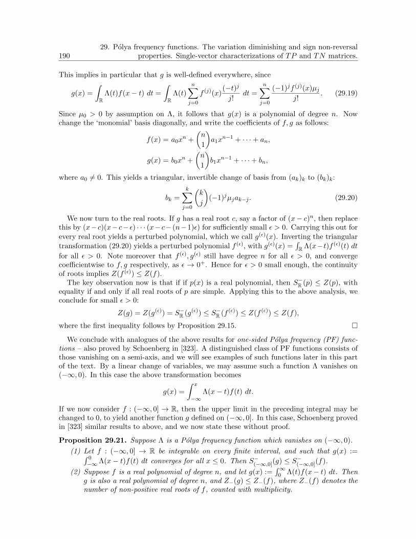
19029. Polya frequency functions. The variation diminishing and sign non-reversal

properties. Single-vector characterizations of TP and TN matrices.

This implies in particular that g is well-defined everywhere, since

g(x) =

∫R

Λ(t)f(x− t) dt =

∫R

Λ(t)

n∑j=0

f (j)(x)(−t)j

j!dt =

n∑j=0

(−1)jf (j)(x)µjj!

. (29.19)

Since µ0 > 0 by assumption on Λ, it follows that g(x) is a polynomial of degree n. Nowchange the ‘monomial’ basis diagonally, and write the coefficients of f, g as follows:

f(x) = a0xn +

(n

1

)a1x

n−1 + · · ·+ an,

g(x) = b0xn +

(n

1

)b1x

n−1 + · · ·+ bn,

where a0 6= 0. This yields a triangular, invertible change of basis from (ak)k to (bk)k:

bk =

k∑j=0

(k

j

)(−1)jµjak−j . (29.20)

We now turn to the real roots. If g has a real root c, say a factor of (x− c)n, then replacethis by (x− c)(x− c− ε) · · · (x− c− (n−1)ε) for sufficiently small ε > 0. Carrying this out for

every real root yields a perturbed polynomial, which we call g(ε)(x). Inverting the triangular

transformation (29.20) yields a perturbed polynomial f (ε), with g(ε)(x) =∫R Λ(x−t)f (ε)(t) dt

for all ε > 0. Note moreover that f (ε), g(ε) still have degree n for all ε > 0, and convergecoefficientwise to f, g respectively, as ε → 0+. Hence for ε > 0 small enough, the continuityof roots implies Z(f (ε)) ≤ Z(f).

The key observation now is that if if p(x) is a real polynomial, then S−R (p) ≤ Z(p), withequality if and only if all real roots of p are simple. Applying this to the above analysis, weconclude for small ε > 0:

Z(g) = Z(g(ε)) = S−R (g(ε)) ≤ S−R (f (ε)) ≤ Z(f (ε)) ≤ Z(f),

where the first inequality follows by Proposition 29.15.

We conclude with analogues of the above results for one-sided Polya frequency (PF) func-tions – also proved by Schoenberg in [323]. A distinguished class of PF functions consists ofthose vanishing on a semi-axis, and we will see examples of such functions later in this partof the text. By a linear change of variables, we may assume such a function Λ vanishes on(−∞, 0). In this case the above transformation becomes

g(x) =

∫ x

−∞Λ(x− t)f(t) dt.

If we now consider f : (−∞, 0] → R, then the upper limit in the preceding integral may bechanged to 0, to yield another function g defined on (−∞, 0]. In this case, Schoenberg provedin [323] similar results to above, and we now state these without proof.

Proposition 29.21. Suppose Λ is a Polya frequency function which vanishes on (−∞, 0).

(1) Let f : (−∞, 0] → R be integrable on every finite interval, and such that g(x) :=∫ 0−∞ Λ(x− t)f(t) dt converges for all x ≤ 0. Then S−(−∞,0](g) ≤ S−(−∞,0](f).

(2) Suppose f is a real polynomial of degree n, and let g(x) :=∫∞

0 Λ(t)f(x− t) dt. Theng is also a real polynomial of degree n, and Z−(g) ≤ Z−(f), where Z−(f) denotes thenumber of non-positive real roots of f , counted with multiplicity.

29. Polya frequency functions. The variation diminishing and sign non-reversalproperties. Single-vector characterizations of TP and TN matrices. 191

29.3. Early results on total non-negativity and variation diminution. We next dis-cuss some of the origins of the variation diminishing property, and its connection to totalnon-negativity. First observe by Theorem 4.1 and Remark 4.4 for Hankel moment matrices,that total non-negativity is implicit in the solution of the Stieltjes moment problem – as alsoin the Routh–Hurwitz criterion for stability; see Theorem 31.3 – both from the 1800s.

Coming to the variation diminishing property: it shows up in the correspondence [118]between Fekete and Polya (published in 1912) that has been mentioned above in the contextof proving the ‘contiguous minor’ test for total positivity of a matrix. (As a bit of trivia:Fekete, Polya, and Szasz were three of the earliest students of L. Fejer; his last student wasVera Sos; and other students include Erdos, von Neumann, Turan, Aczel, Egervary, Toth,and Marcel Riesz, among others.)5

We now discuss a result of Fekete from his correspondence with Polya, which not onlydealt with variation diminution but also gave rise to the notion of Polya frequency sequences– discussed in the next section.

A common, historical theme underlying this section and the next, as well as Section 33below (on the Laguerre–Polya–Schur program), involves understanding real polynomials andtheir roots. In fact this theme dates back to Descartes, who in his 1637 work [100] proposedhis ‘Rule of Signs’ – see e.g. Lemma 5.2. The question of understanding the roots remainedpopular (and does so to this day; see Section 33). As a notable example, we recall Laguerre’s1883 paper [229], which deals with this theme, and opens by recalling Descartes’ rule of signsand proving it using Rolle’s theorem (the ‘standard’ proof these days). In [229], Laguerre usedthe word ‘variations’ to denote the sign changes in the Maclaurin coefficients of a polynomialor power series. Among the many results found in his memoir, we list two:

Theorem 29.22 (Laguerre, 1883, [229]).

(1) Given an interval [a, b] ⊂ R and an integrable function Φ : [a, b]→ R, the number of

zeros of the Fourier–Laplace transform∫ ba e−sxΦ(x) dx is at most the number of zeros

of the antiderivative∫ ta Φ(x) dx for t ∈ [a, b].

(2) Suppose f(x) is a polynomial. Then the number of variations (sign changes in theMaclaurin coefficients) of the power series esxf(x) is a non-increasing function ofs ∈ [0,∞), and is uniformly bounded below by the number of positive roots of f .

In particular, in part (2), the variation for any s > 0 is ‘diminishing’, and always finite, sinceit is bounded above by the variation at s = 0.

Especially this latter result was pursued by Fekete, who wrote to Polya to the effect that“Laguerre did not fully justify” Theorem 29.22(2) in his work [229]. To address this, Feketeconsidered a formal power series with real coefficients c0 + c1t+ · · · , acting by multiplicationon the space of such power series. With respect to the standard basis of monomials, this

5As another bit of trivia, the descendants of K.T.W. Weierstrass and E.E. Kummer feature prominentlyin the study of (total) positivity. Their joint students include:

(1) F.G. Frobenius and L.I. Fuchs, who in turn mentored I. Schur, who was the advisor of I.J. Schoenberg;(2) L. Konigsberger, who mentored G. Pick, who advised C. Loewner; and(3) L. Fejer, who mentored G. Polya and M. Fekete.

19229. Polya frequency functions. The variation diminishing and sign non-reversal

properties. Single-vector characterizations of TP and TN matrices.

transformation is given by the triangular matrix

Tc :=

c0 0 0 · · ·c1 c0 0 · · ·c2 c1 c0 · · ·...

......

. . .

Fekete then stated the following result on variation diminution (a term coined by Polya)

– further asserting that it could be used to prove Theorem 29.22(2):

Proposition 29.23 (Fekete, 1912, [118]). Suppose for an integer p ≥ 2 that the matrixTc (supported on Z≥0 × Z≥0) is TNp – i.e., every finite submatrix is TNp. Given a vectorx = (x0, x1, . . . , xp−1, 0, 0, . . . )

T (the coefficients of a polynomial), we have S−(Tcx) ≤ S−(x).

Note here that Tcx represents the coefficients of a formal power series, and hence can forma sequence with infinitely many non-zero terms. Nevertheless, every such sequence has fewersign changes than the finite sequence x. (To deduce Laguerre’s result, Fekete showed thatfor s ≥ 0, Proposition 29.23 applies to the special case ck = sk/k!. See Section 30.4.)

Thus, we have journeyed from Descartes (1637), to Laguerre (1883), to Fekete (1912), toSchoenberg (1930) and Motzkin (1936) – see Theorem 3.22 from Motzkin’s thesis and thepreceding paragraph – to Schoenberg (1951), in studying the origins of variation diminutionand subsequent developments. (This omits, with due apologies, the substantial contributionsof Gantmacher, Krein, and others; the connections to the work of Sturm and to Sturm–Liouville eigenvalue problems; as well as the 1915 paper [284] of Polya, which proved adifferent variation-diminishing property of PF functions on polynomials, led Schoenberg tocoin the phrase ‘Polya frequency functions’, and is briefly discussed in Section 34.) CertainlyFekete’s result and the aforementioned developments led Schoenberg and Gantmacher–Kreinto develop the theories of total positivity, Polya frequency functions, and variation diminution.

We conclude this historical section with yet another connection between total non-negativityand Descartes’ rule of signs. In his 1934 paper [311] in Math. Z., Schoenberg proved the fol-lowing result. In it, we use the notation that a finite sequence f0, f1, . . . , fn of functions obeysDescartes’ rule of signs in an open sub-interval (a, b) ⊂ R if the number of zeros in (a, b) ofthe nontrivial real linear combination

c0f0(x) + · · ·+ cnfn(x), cj ∈ R,n∑j=0

c2j > 0

is no more than the number of sign changes in the sequence (c0, . . . , cn).

Theorem 29.24 (Schoenberg, [311]). Fix a sequence of real polynomials pj(x) := aj0+aj1x+· · ·+ ajjx

j for 0 ≤ j ≤ n, with all ajj > 0. The following are equivalent:

(1) The sequence (p0, . . . , pn) obeys Descartes’ rule of signs in (0,∞).

(2) The upper triangular matrix

a00 a10 · · · an0

a11 · · · an1

. . ....ann

is totally non-negative.

(E.g., for the ‘usual’ Descartes’ rule of signs, this matrix is precisely the identity matrix.)Schoenberg also extended Descartes and Laguerre’s results to more general domains in C; seehis 1936 paper [313] in Duke Math. J.

29. Polya frequency functions. The variation diminishing and sign non-reversalproperties. Single-vector characterizations of TP and TN matrices. 193

29.4. The sign non-reversal property. We now discuss another fundamental – and veryrecent – characterization of total positivity. To motivate this result, begin with Schoenberg’s1930 result asserting that every TN matrix has the variation diminishing property. Fromhere, it is natural to proceed in two directions:

(1) Characterize all matrices with the variation diminishing property. This was carriedout by Motzkin in his 1936 thesis; see Theorem 3.22.

(2) Find additional conditions that, together with the variation diminishing property,characterize TN and TP matrices. This was carried out in Theorems 29.8 and 29.11,and involves a ‘sign non-reversal’ phenomenon.

Our goal here is to show that in fact, it is the variation diminishing property that is notnecessary in Theorems 29.8 and 29.11. To proceed, we isolate the key notion into the followingdefinition.

Definition 29.25. Fix integers n ≥ 1.

(1) A square real matrix An×n has the sign non-reversal property on a set of vectorsS ⊂ Rn, if for all non-zero vectors x ∈ S there exists a coordinate j ∈ [n] such thatxj(Ax)j > 0. If the set S is not specified, it is taken to be Rn.

(2) We also require the non-strict sign non-reversal property for a matrix A ∈ Rn×n, ona set of vectors S ⊂ Rn. This says that for all 0 6= x ∈ S there exists a coordinatej ∈ [n] such that xj 6= 0 and xj(Ax)j ≥ 0.

(3) Define Rnalt to be the open bi-orthant consisting of the vectors in Rn whose coordinatesare all non-zero and have alternating signs.

(4) Finally, define dr := (1,−1, . . . , (−1)n−1)T ∈ Rnalt.

With these notions defined, in their recent work in Bull. London Math. Soc., Choudhury,Kannan, and Khare have characterized TP/TN matrices purely in terms of their sign non-reversal property. More strongly:

Theorem 29.26 ([81]). Fix integers m,n ≥ p ≥ 1 and a real matrix A ∈ Rm×n. Thefollowing are equivalent:

(1) The matrix A is TPp.(2) Every square submatrix B of A of size r ∈ [1, p] has the sign non-reversal property.(3) Every contiguous square submatrix B of A of size r ∈ [1, p] has the sign non-reversal

property on Rralt ⊂ Rr.

A part of this theorem was previously shown in 1966 by Ky Fan [114]. Also note that(2) =⇒ (3), so we will show (1) =⇒ (2) and (3) =⇒ (1). The latter implication canbe weakened even further, to require the sign non-reversal property for a single alternatingvector (chosen from an orthant) – the same orthant as in Theorem 29.9. This was shownvery recently:

Theorem 29.27 (Choudhury, [80]). The three conditions above are further equivalent to:

(4) For each contiguous square submatrix B of A of size r ∈ [1, p], and any choice of vector0 6= vB := (α1,−α2, . . . , (−1)r−1αr)

T with all αj ≥ 0, B has the sign non-reversalproperty for zB := adj(B)vB, where adj(B) is the adjugate matrix of B.

(As the proof will reveal, one can also work with −vB instead of vB.) Following the proofof these results, we will show that Am×n is TNp if and only if every square submatrix of size≤ p satisfies a condition similar to this one. See Theorem 29.28 and the subsequent result.

19429. Polya frequency functions. The variation diminishing and sign non-reversal

properties. Single-vector characterizations of TP and TN matrices.

Proof. We first show that (1) implies the sign non-reversal property on vectors with non-negative coordinates – under the weaker assumption of working only with the positivity of theprincipal minors of B, of size≤ r. (Such matrices are called P -matrices; see e.g. [105, 121, 134]for this argument.) The result is by induction on r ≥ 1, with the r = 1 case obvious. Supposethe result holds for all (r − 1) × (r − 1) real matrices with positive principal minors. Nowlet Br×r have the same property, with x,−Bx ∈ Rr having all non-negative coordinates. Weneed to prove x = 0.

By choice (and Cramer’s rule), B−1 has positive diagonal entries. Let b denote the firstcolumn of B−1, and define

θ := minj∈[r]:bj>0

xjbj,

noting that the minimum is taken over a non-empty set. Hence it is attained: 0 ≤ θ = xj0/bj0at some j0 ∈ [r]. Then y := x− θb has non-negative coordinates, by choice of θ, and it hasj0th coordinate zero. But we also have

−By = −Bx+ θBb = −Bx+ θe1,

and this has non-negative coordinates again.We now claim y = 0. Indeed, if we obtain y′ by deleting the j0th coordinate, and B′ by

deleting the j0th row and column, then an easy verification yields that −B′y′,y′ have non-negative coordinates. By the induction hypothesis, y′ = 0, whence y = 0. But then Bx = θe1

has non-negative coordinates. Since so does −Bx, we have Bx = 0. Since det(B) > 0, weobtain x = 0. This completes the proof of (1) =⇒ (2) by induction – for x with non-negativecoordinates.

Now suppose x ∈ Rr and xj(Bx)j ≤ 0 for all j. Let J ⊂ [r] index the negative coordinates

of x, and define the diagonal matrixDJ with (k, k) entry (−1)1(k∈J). If now xj and (Bx)j haveopposite signs for all j (meaning their product is non-positive), then so do (eTj D)x = eTj (Dx)

and (eTj D)(Bx) = eTj (DBD)(Dx). Thus Dx, (DBD)(Dx) have corresponding coordinatesof opposite signs. As DBD also has all principal minors positive, the above analysis impliesDx = 0, and so x = 0. Hence (1) =⇒ (2) for all vectors x ∈ Rr.

(Though we do not require it, we also mention quickly why (2) =⇒ (1). Let B be anysquare submatrix of A; as the set of non-real eigenvalues is closed under conjugation, theirproduct is strictly positive. It thus suffices to show that every real eigenvalue is positive.By the sign non-reversal property, if Bx = λx with λ ∈ R and x ∈ Rr, and if xj 6= 0, thenxj(Bx)j = λx2

j > 0, whence λ > 0.)

Next, that (2) =⇒ (3) =⇒ (4) is immediate. Finally, suppose (4) holds. By the Fekete–Schoenberg lemma 4.9, it suffices to show that all contiguous r × r minors are positive, for1 ≤ r ≤ p. The proof is by induction on r ≤ p; the r = 1 case directly follows from (4) usingr = 1 and B1×1 = (ajk), using that adj(B) = (1).

For the induction step, suppose Br×r is a contiguous square submatrix of A, with r ≤ p,and all contiguous minors of B of size ≤ r − 1 are positive. Then the same holds for allproper minors of B by Lemma 4.9, and so adj(B) is a matrix with a ‘checkerboard’ patternof signs: sgn(adj(B)jk) = (−1)j+k for 1 ≤ j, k ≤ r. It follows for any vB 6= 0 as specified that

zB = adj(B)vB ∈ Rralt. Now compute for j0 ∈ [1, r]:

0 < (zB)j0 · (BzB)j0 = (−1)j0−1|(zB)j0 | · (detB)(vB)j0 = det(B)|(zB)j0 |αj0 .

It follows that all three factors are non-zero, and detB > 0, which completes the proof.

29. Polya frequency functions. The variation diminishing and sign non-reversalproperties. Single-vector characterizations of TP and TN matrices. 195

The final results here, again by Choudhury–Kannan–Khare and Choudhury (2021), char-acterize TNp matrices through their sign non-reversal:

Theorem 29.28 ([81]). Fix integers m,n ≥ p ≥ 1 and a real matrix A ∈ Rm×n. Thefollowing are equivalent:

(1) The matrix A is TNp.(2) Every square submatrix B of A of size r ∈ [1, p] has the non-strict sign non-reversal

property on Rr.(3) Every square submatrix B of A of size r ∈ [1, p] has the non-strict sign non-reversal

property on Rralt.

As in Theorem 29.27(4) above, this can be further weakened:

Theorem 29.29 (Choudhury, [80]). The preceding three conditions are further equivalent to:

(4) Every square submatrix B of A of size r ∈ [1, p], has the non-strict sign non-reversalproperty for the single vector zB := adj(B)vB, where vB ∈ Rralt is arbitrarily chosen.

Proof. First suppose (1) holds. By Whitney’s density theorem 6.7 there is a sequence A(l)

of TPp matrices converging entrywise to A. Now given B, let B(l)r×r be the submatrix of A(l)

indexed by the same rows and columns as B. Now fix a vector 0 6= x ∈ Rr, and index byJ ⊂ [r] the non-zero entries in x. Since B(l) is TP , by Theorem 29.26 there exists jl ∈ [r]

such that xjl(B(l)x)jl > 0; moreover, jl ∈ J ∀l. As J is finite, there exists j0 ∈ [r] and an

increasing subsequence of positive integers lq such that jlq = j0 for all q ≥ 1. Now (2) follows:

xj0(Bx)j0 = limq→∞

xjlq (B(lq)x)jlq ≥ 0, xj0 6= 0.

(The proof of (2) =⇒ (1) is essentially the same as in the preceding proof, with λx2j ≥ 0

now; once again, we do not require it.) That (2) =⇒ (3) =⇒ (4) is immediate. Finally,assume (4) and claim by induction on r ≤ p, that every r × r minor of A is non-negative.The base case is immediate; for the induction step, let Br×r be a submatrix of A, and assumethat all (r − 1) × (r − 1) minors of B are non-negative. If detB = 0 then we are done; elseassume B is invertible. Now no row or column of adj(B) is zero, and adj(B)jk is either zero

or has sign (−1)j+k for all j, k. Thus, adj(B)vB ∈ Rralt. Now a similar computation as in thepreceding proof shows that for some j0 ∈ [1, r], we have by (4):

0 ≤ (B adj(B)vB)j0(adj(B)vB)j0 = (detB)vBj0zBj0 .

Since all factors here are non-zero and vBj0 , zBj0

have the same sign, it follows that detB > 0,and so we are done by induction.

Remark 29.30. In this section, we have seen classical results which help characterize totallypositive/non-negative matrices A using the variation diminishing property and the sign non-reversal property – both of which involve certain conditions holding for all vectors in Rn. Wealso explained recent results of Choudhury [80, 81] that provided single test vectors, one forevery (contiguous) submatrix of A. In [80], Choudhury also provides a third characterizationof total positivity – via the Linear Complementarity Problem, which has applications inbimatrix games, linear programming, and other areas. Once again, he is able to improve thischaracterization to use a single test vector. See [80] for details.

30. Polya frequency sequences and their generating functions. 197

30. Polya frequency sequences and their generating functions.

In this section, we introduce and study Polya frequency sequences, and take a look at root-location phenomena for their generating functions. Recall Fekete’s proposition 29.23 (1912)from the preceding section, on the variation diminishing property of TNp triangular Toeplitzmatrices that are supported on Z× Z. Such matrices are now known as PF sequences:

Definition 30.1.

(1) A real sequence a = (an)n∈Z is a Polya frequency (PF) sequence if the associatedToeplitz kernel Ta : Z× Z→ R, sending (x, y) 7→ ax−y, is TN .

(2) The PF sequence a is said to be one-sided if there exist n± ∈ Z such that an = 0either for all n < n− or for all n > n+ (or both).

(3) More general is the notion of a p times (i.e., multiply) positive sequence, or a TNp

sequence a, which corresponds to the matrix Ta : Z × Z → R being TNp. (This toohas a one-sided version, as above.)

For instance, one can specialize the results of Section 28.2 to X = Y = Z, to obtaincharacterizations of TNp sequences or PF sequences.

30.1. Examples. We begin by studying examples of PF sequences, and of the subclass ofone-sided PF sequences (TN or TNp). Clearly, every constant (non-negative) sequence an ≡ cfor c ≥ 0 is a PF sequence. Our first source of non-constant PF sequences comes from Polyafrequency functions:

Lemma 30.2. If Λ : R→ R is a PF function, or even a TN function, then (Λ(an+ b))n∈Zis a PF sequence for a, b ∈ R. If a 6= 0 and Λ is TP , then so is (Λ(an+ b))n∈Z.

Proof. If a = 0 then the result is immediate. Now suppose a 6= 0, and x,y ∈ Zp,↑ for somep ≥ 1. Then the p× p matrix

(Λ(a(xj − yk) + b))pj,k=1 =

TΛ[ax + b1; ay], if a > 0,

TΛ[|a|y + b1; |a|x]T , if a < 0,

and both choices have non-negative determinant. The final assertion is showed similarly.

Another elementary result is the closure of the set of TNp sequences. The proof is easy.

Lemma 30.3. Suppose p ≥ 1 and a(k) = (a(k)n )n∈Z is a TNp sequence for all k ≥ 1. If

a(k) → a pointwise as k →∞, then a is also TNp.

The above lemmas allow one to ‘draw’ PF sequences from PF functions, along any infinitearithmetic progression. Here are two examples:

Example 30.4. For a real number q > 0, the sequences (qn)n∈Z and (qn1n≥0)n∈Z are bothPF sequences. The former is because (qxj−yk)nj,k=1 is a rank-1 matrix with positive entries

for any choice of integers xj , yk, so TN . If q ∈ (0, 1), then the latter kernel is drawn fromλ1(x) = e−x1x≥0 (which is shown in Example 32.11 below to be a PF function), at thearguments x = −n log(q). If q > 1 then it is drawn from fc(x) = ecxλ1(x) at the argumentsn log(q) and with c = 2. (By Lemma 28.3, fc is now a TN function as well.) Finally, if q = 1then it is drawn from the Heaviside kernel

H1(x) = 1x≥0 = limc→1

fc(x)

at any infinite arithmetic progression. (Alternately, for all q one can use the analysisabove (30.10), later in this section.)

198 30. Polya frequency sequences and their generating functions.

Example 30.5. For a real number q ∈ (0, 1), the sequence (qn2)n∈Z is a TP PF sequence.

Indeed, this sequence is drawn from the Gaussian PF function Gσ for σ = − log(q) > 0 (seeExample 29.4).

30.2. Generating functions and representation theorem for one-sided PF sequences.Given a real sequence a = (an)n≥0 of finite or infinite length, it is natural to encode it by thecorresponding generating function

Ψa(x) =∑n≥0

anxn.

When the sequence (. . . , 0, 0, a0, a1, a2, . . . ) is a TNp sequence, and only finitely many termsan are non-zero, one can deduce results about the locations of the roots of the correspondinggenerating polynomial Ψa(x) – and in turn, use this information to classify all finite TNsequences. We carry out this analysis in the present subsection and the next; it will be usefulin the next part of this text, in classifying the preservers of total positivity for PF sequences.The present subsection ends by revealing the most general form of the generating function ofone-sided PF sequences.

Proposition 30.6. Suppose (an)n∈Z is TN2, shifted and normalized such that a0 = 1.

(1) If ak = 0 for some k > 0 (respectively k < 0), then al = 0 for all l > k (respectivelyl < k).

(2) If an = 0 for all n < 0, and the sequence a is TNp for some p ≥ 2, then its generatingfunction Ψa has a non-zero radius of convergence.

(3) If an = bn = 0 for all n < 0, and a,b are TNp sequences, then so is the sequence ofMaclaurin coefficients of Ψa(x)Ψb(x).

(4) If an = 0 for all n < 0, and a is TN , then so is the sequence of Maclaurin coefficientsof 1/Ψa(−x).

Note that the final assertion here does not go through if we assume a to be merely TNp

and not TN ; see e.g. [293]. Also note the similarity of the first assertion to Theorem 28.4.

Proof. The first part is easy to check: given integers k,m with ak = 0, note that

detTa[(k, k +m); (0, k)] = det

(ak a0

ak+m am

)= −ak+m.

Now if 0 < k,m then work with this matrix; if 0 > k,m then reverse its rows and columns.Either way, the non-negativity of the determinant implies ak+m = 0 for all m > 0 (or allm < 0), as desired.

For the second part, if only finitely many terms are non-zero then the result is obvious;otherwise by the first part, an > 0 for all n ≥ 0. Now given n ≥ 1, we have

0 ≤ detTa[(n, n+ 1); (0, 1)] = det

(an an−1

an+1 an

)= a2

n − an+1an−1.

From this it follows that an+1/an > 0 is non-increasing in n. Let β1 ≥ 0 be the infimum/limitof this sequence of ratios; then the power series Ψa(x) =

∑n≥0 anx

n has radius of convergence

1/β1, by basic calculus.To show the third part, first observe that the Z×Z Toeplitz matrices Ta, Tb are both TNp

by definition. Moreover, their product is a well-defined, lower-triangular Toeplitz matrix byinspection, and corresponds precisely to ‘convolving’ the two sequences. But this ‘convolution’also corresponds to multiplying the two generating functions. Thus, it suffices to show thatTaTb is TNp. This follows by the Cauchy–Binet formula (see Theorem 5.5).

30. Polya frequency sequences and their generating functions. 199

Finally, for the fourth part, the reciprocal of Ψa(x) has a positive radius of convergencearound 0, by basic calculus. Develop the reciprocal around 0, on the interval of convergence:

1

Ψa(x)=∑n≥0

bnxn.

Denote the tuple of coefficients by b. By the arguments used to prove the previous part, thisyields the lower triangular Toeplitz matrix Tb (indexed by Z× Z) such that TaTb = TbTa =IdZ×Z. Since Ta is TN , we claim that so is the matrix with (j, k) entry (−1)j+kbj−k =

(−1)j−kbj−k – which is precisely Tc for cn = (−1)nbn. But this would correspond to thedesired generating function: ∑

n≥0

(−1)nbnxn =

1

Ψa(−x).

It thus remains to prove the above claim. This requires the well-known Jacobi complemen-tary minor formula [190]: given integers 0 < p < n, an invertible n × n matrix A (over a

commutative ring), and equi-sized subsets J,K ∈ [n]p,↑,

detA · det(A−1)Kc×Jc = (−1)j1+k1+···+jp+kp detAJ×K . (30.7)

where Jc := [n] \ J , and similarly for Kc.We first quickly sketch the proof of this result (via an argument found on the internet); by

pre- and post- multiplying A by suitable permutation matrices, one can reduce to the case ofJ = K = [p] – in which case the sign on the right is +1. Now let Aj denote the jth column

of A, and A−1j of A−1 respectively. Writing ej for the standard basis of Rn, we have:

A[e1| · · · |ep|A−1

p+1| · · · |A−1n

]= [A1| · · · |Ap|ep+1| · · · |en] .

This can be rewritten as:(AJ×K AJ×Kc

AJc×K AJc×Kc

)(Idp×p A−1

K×Jc0 A−1

Kc×Jc

)=

(AJ×K 0AJc×K Id(n−p)×(n−p)

).

Taking the determinant of both sides proves Jacobi’s result for J = K = [p].To conclude the proof of the fourth part, we now use Jacobi’s identity to prove the afore-

mentioned claim (in bold). Let M be a square submatrix of Tc, with cn = (−1)nbn as above.There exists a suitably large principal submatrix B′ of Tc, indexed by contiguous rows andcolumns, of which M is a p×p submatrix for some p. Let A be the corresponding ‘contiguous’principal submatrix of Ta. Multiplying every row and column of B′ indexed by even numbersby −1, we obtain a matrix B such that AB = Id. Finally, let N be the ‘complementary’submatrix of A, indexed by the rows and columns not indexing M in B (or in B′). ApplyingJacobi’s identity and carefully keeping track of signs shows that det(M) ≥ 0, as desired.

We now proceed toward the form of the generating series Ψa for an arbitrary one-sidedPolya frequency sequence. First consider the case when a contains only finitely many non-zeroterms, which by Proposition 30.6 must be ‘consecutive’. In other words,

a = (. . . , 0, 0, a0, . . . , am, 0, 0, . . . ), m ≥ 0, a0, . . . , am > 0.

Lemma 30.8. With a as above, if m = 0 or m = 1 (with a0, am arbitrary positive scalars),then a is a PF sequence. In particular, if Ψa(x) is a polynomial with all roots in (−∞, 0),then a is a PF sequence.

200 30. Polya frequency sequences and their generating functions.

Proof. First let m = 0, 1, and suppose a square submatrix M of Ta has neither a zeroinitial/final row nor column. For m = 0, the only possible alternative is that M is a diagonalmatrix, with determinant a power of a0 > 0. For m = 1, there are two alternatives: allentries along the main diagonal of M are a0 (whence the sub-diagonal has all entries a1, andall other entries in M are zero), or they are all a1 (whence the super-diagonal has all entriesa0, and all other entries in M are zero). Both cases yield detM > 0.

Now suppose Ψa(x) is a polynomial with all roots in (−∞, 0). Writing this as am(x +β1)(x+β2) · · · (x+βm) (with −βj the roots of Ψa), we note by the preceding paragraph thatx+βj = Ψ(...,0,βj ,1,0,... ) is the generating polynomial of a PF sequence, as is am = Ψ(...,0,am,0,... ).

Therefore, so is their product = Ψa(x), by Proposition 30.6(3).

Example 30.9. Let δ ≥ 0. Lemma 30.8 and Proposition 30.6(3) show that the finite sequenceam with Ψam(x) = (1 + δx/m)m is a PF sequence. Taking limits via Lemma 30.3, thesequence an = 1n≥0δ

n/n! now forms a PF sequence, since its generating power series isΨa(x) = eδx = limm→∞(1 + δx/m)m.

We now make some deductions from the above results in this section. Choose scalars δ ≥ 0,as well as αj , βj ≥ 0 for integers j ≥ 1 such that

∑j(αj + βj) < ∞. Then

∏nj=1(1 + αjx)

generates a PF sequence for all n ≥ 1, by Lemma 30.8 and Proposition 30.6. Take the limitas n→∞; since |1 + αjx| < eαj |x| and

∑j αj <∞, the limit, given by

∞∏j=1

(1 + αjx)

is an entire function, which generates a PF sequence by Lemma 30.3. Similarly, 1/(1− βjx)generates an infinite one-sided PF sequence for each j ≥ 1, by Lemma 30.8 and Proposi-tion 30.6(4). (For a far easier proof for (1 − βjx)−1, one can instead use Example 32.10below to show this assertion for βj = 1, then deduce the case of general βj by pre- and post-multiplying a given submatrix by diagonal matrices having suitable powers of βj .) It followsas above that 1/

∏∞j=1(1− βjx) also generates a PF sequence. Applying Proposition 30.6(3),

eδx∞∏j=1

1 + αjx

1− βjx, where αj , βj , δ ≥ 0,

∞∑j=1

(αj + βj) <∞ (30.10)

is the generating function of a one-sided Polya frequency sequence a, with a0 = 1.Remarkably, this form turns out to encompass all one-sided Polya frequency sequences.

This is a deep result, shown in a series of papers [4, 5, 106, 107] by Aissen–Schoenberg–Whitney and Edrei – separately and together – and is stated here without proof.

Theorem 30.11 (Aissen–Edrei–Schoenberg–Whitney, 1951–52). A function∑∞

n=0 anxn with

a0 = 1, is the generating function Ψa(x) for a one-sided Polya frequency sequence a =(a0, a1, . . . ) if and only if Ψa is of the form (30.10).

(As a historical remark: Whitney was Schoenberg’s student, while Aissen and Edrei werestudents of Polya.) For proofs, the reader can either look into the aforementioned papers, orfollow the treatment in Karlin [200, Chapter 8]; one also finds there a representation theoremfor the generating function of a two-sided PF sequence. The proof involves using ideas ofHadamard from his 1892 dissertation [158], as well as Nevanlinna’s refinement of Picard’stheorem [269].

30. Polya frequency sequences and their generating functions. 201

Remark 30.12. For completeness, we refer the reader to the recent paper [104], in which Dy-achenko proves similar representation results involving the total non-negativity of generalizedHurwitz-type matrices.

Remark 30.13. Also for completeness, we mention the analogous, ‘two-sided’ result:An arbitrary real sequence (an)n∈Z is a Polya frequency sequence if and only if it is either

of the form (aρn)n∈Z with a, ρ > 0; or else its generating Laurent series converges in someannulus r1 < |z| < r2 with 0 ≤ r1 < r2, and has the factorization∑

n∈Zanz

n = Ceaz+a′z−1

zm∞∏j=1

(1 + αjz)(1 + α′jz−1)

(1− βjz)(1− β′jz−1),

where C ≥ 0, m ∈ Z, a, a′, αj , βj , α′j , β′j ≥ 0 and

∑j(αj + βj + α′j + β′j) <∞.

The ‘if’ part was proved by Schoenberg [321], and the harder, ‘only if’ part was shown byEdrei [108].

This part concludes by specializing to the case where Ψa has integer coefficients. Here werefer to papers by Davydov [99] and Ho Hai [177], in which they show that the Hilbert seriesof a quadratic R-matrix algebra (over a field of characteristic zero) generates a PF sequence.The result relevant to this text is:

Theorem 30.14 (Davydov). A power series Ψa(x) ∈ 1 + xZ[[x]] generates a PF sequence aif and only if Ψa has the form (30.10), with δ = 0 and all but finitely many αj , βj also zero.

30.3. Application 1: (Dual) Jacobi–Trudi identities. We now provide some applica-tions of the above results. The first is to algebra and symmetric function theory. As mentionedabove, Theorem 30.14 was applied to the theory of quadratic R-matrix algebras over a field ofcharacteristic zero. We briefly touch upon this area, starting with two examples of this phe-nomenon, which are Hilbert series of two well-known quadratic (and Koszul dual) algebras.Recall that for a Z≥0-graded algebra A := ⊕n≥0An with finite-dimensional graded pieces, itsHilbert series is H(A, x) :=

∑n≥0 x

n dimAn. Now suppose V is a finite dimensional vectorspace, say of dimension m. The Hilbert series of its exterior algebra ∧•V is

H(∧•V, x) = (1 + x)m,

and this is the generating function of a (finite, binomial) PF sequence by the above results.These results also imply the same conclusion for the Hilbert series of the symmetric algebra:

H(S•V, x) =1

(1− x)m.

More generally, one fixes an operator, or R-matrix R : V ⊗ V → V ⊗ V , which satisfiestwo conditions:

• The Yang–Baxter equation R12R23R12 = R23R12R23, i.e.,

(R⊗ Id)(Id⊗R)(R⊗ Id) = (Id⊗R)(R⊗ Id)(Id⊗R) on V ⊗ V ⊗ V.

• The Hecke equation (R + Id)(R − q Id) = 0, where q is a non-zero element in theunderlying ground field.

Associated to this R-matrix, define two Z≥0-graded algebras, by quotienting the tensoralgebra by two-sided ‘quadratic’ ideals:

(1) The R-exterior algebra is ∧•R(V ) := T •(V )/(im(R+ Id)).(2) The R-symmetric algebra is S•q,R(V ) := T •(V )/(im(R− q Id)).

202 30. Polya frequency sequences and their generating functions.

(For example, if R is the flip operator v1 ⊗ v2 7→ v2 ⊗ v1 and q = 1, then we obtain the usualexterior and symmetric algebras above.) It is well-known that the Hilbert series H(∧•R(V ), x)and H(S•q,R(V ),−x) are reciprocals of one another. In this general setting, Davydov [99] and

Ho Hai [177] showed:

Proposition 30.15. Let V be finite-dimensional over a field of characteristic zero, q a scalareither equal to 1 or not a root of unity, and R : V ⊗V → V ⊗V an R-matrix as above. Thenthe Hilbert series H(∧•R(V ), x), whence H(S•q,R(V ), x) (by Proposition 30.6(4)), generates aPF sequence.

These results by Davydov and Ho Hai hold in the case when the underlying ‘Iwahori–Hecke algebra’ (which operates on tensor powers V ⊗n via the R-matrix) is semisimple, whichhappens when 1 + q + · · ·+ qn−1 6= 0 for all n > 0. We add for completeness that when q isa root of unity instead, such a result was proved very recently by Skyrabin [339] under anadditional hypothesis: the “1-dimensional source condition”.

We now move from algebra to algebraic combinatorics. Restrict to the special case of Rbeing the flip operator and q = 1; but now allow for V to have a ‘multigraded’ basis vjwith degree αjx, where αj > 0 for j ≥ 1. This leads to distinguished objects in algebraiccombinatorics. Indeed, the Hilbert series is now the polynomial Ψa(x) = (1 + α1x) · · · (1 +αmx), with α1, . . . , αm > 0 (so a0 = 1) – so a0, a1, . . . , am are precisely the elementarysymmetric polynomials aj = ej(α1, . . . , αm) in the roots αk.

Taking limits as in the above analysis in this section, if αj ≥ 0 and∑∞

j=1 αj < ∞,

then aj = ej(α1, α2, . . . ) for all j ≥ 0. Here, the mth elementary symmetric polynomial in(in)finitely many variables u1, u2, . . . is defined to be

ej(u) :=∑

1≤k1<k2<···<kj

uk1 · · ·ukj ,

with e0(u) := 1 and ej(u) := 0 if u has fewer than j entries.In fact a stronger phenomenon occurs: if we replace the αj by variables u = (u1, u2, . . . ),

then every minor of the infinite triangular Toeplitz matrix1 0 0 0 · · ·

e1(u) 1 0 0 · · ·e2(u) e1(u) 1 0 · · ·e3(u) e2(u) e1(u) 1 · · ·

......

......

. . .

(30.16)

is monomial positive, meaning that any minor drawn from it is a non-negative sum of mono-mials in the uj . In fact an even stronger result is true: the above matrix is a (skew) Schurpolynomial in the uj . In particular, it is (skew) Schur positive (i.e., a non-negative sum ofSchur polynomials). This phenomenon is known as the dual Jacobi–Trudi identity, and is ina sense, the ‘original’ case of numerical positivity being monomial positivity – in fact, beingSchur positivity. See Appendix F for more on this. (We will see another, more recent suchinstance in Theorem 44.6, which follows from a more general Schur positivity phenomenonshown by Lam–Postnikov–Pylyavskyy [231].)

An analogous phenomenon holds for the ‘usual’ Jacobi–Trudi identity. Namely, supposeΨa(x) = ((1− α1x) · · · (1− αmx))−1 for scalars αk > 0 (so once again, a0 = 1). Then

30. Polya frequency sequences and their generating functions. 203

a0, a1, . . . are precisely the complete homogeneous symmetric polynomials

aj = hj(α1, . . . , αm) :=∑

1≤k1≤k2≤···≤kj

αk1 · · ·αkj , j ≥ 1

and h0(α1, . . . , αm) := 1. Now take limits as above, with αj ≥ 0 and∑∞

j=1 αj <∞ to obtain

aj = hj(α1, α2, . . . ) for j ≥ 0.Once again, a stronger phenomenon than ‘numerical total non-negativity’ holds: if one

replaces the αj by variables u = (u1, u2, . . . ) as above, then every minor of the infiniteToeplitz matrix

1 0 0 0 · · ·h1(u) 1 0 0 · · ·h2(u) h1(u) 1 0 · · ·h3(u) h2(u) h1(u) 1 · · ·

......

......

. . .

(30.17)

is monomial positive, – and more strongly, (skew) Schur positive. Thus, total positivityconnects to the Jacobi–Trudi identity.

30.4. Application 2: Results of Fekete and Laguerre. We now complete the proof ofa result by Laguerre in the preceding section, as promised there. The first step is to prove astrengthening of a weaker version of Fekete’s Proposition 29.23:

Proposition 30.18. Suppose T : Z≥0 × Z≥0 → R is TNp, for some integer p ≥ 2. Given areal vector x = (x0, . . . , xp−1, 0, 0, . . . )

T , we have S−(Tx) ≤ S−(x).

Proof. Suppose S−(Tx) > S−(x) for some finite vector x = (x0, x1, . . . )T with xp = xp+1 =

· · · = 0. Then there exists an initial segment y of Tx of length m + 1 such that S−(y) >S−(x). Let x′ := (x0, . . . , xp−1)T , and let the submatrix T ′ := (tjk)j≤m, k<p. Then T ′ is TNby assumption, and y = T ′x′, so by the variation diminishing property (Theorem 29.11),S−(y) = S−(T ′x′) ≤ S−(x′) = S−(x), a contradiction.

Using this result, we now prove Laguerre’s result as mentioned by Fekete in [118] – butusing finite matrices instead of power series:

Proof of Theorem 29.22(2). For s > 0, let Ts denote the infinite Toeplitz matrix with (j, k)entry sj−k/(j−k)! if j ≥ k, and 0 otherwise. This corresponds to the sequence with generatingfunction esx, so by Example 30.9 the matrix Ts is TN ; moreover, the map esx 7→ Ts, s ≥ 0is a homomorphism of monoids under multiplication.

We now turn to the proof. Applying Proposition 30.18, S−(Tsx) ≤ S−(x) for any finitevector x (padded by infinitely many zeros). In particular, the integers S−(Tsx) : s > 0 areuniformly bounded above by S−(x) < ∞. Moreover, S−(Tsx) and S−(x) are precisely thenumber of variations in the functions esxΨx(x) and Ψx(x), respectively.

We first show that S−(Ts+tx) ≤ S−(Tsx) if s, t > 0. Given m ≥ 0 and s > 0, let T(m)s

represent the leading principal (m+1)×(m+1) submatrix of Ts; and let x(m) = (x0, . . . , xm)T

as above. Since S−(Tsx) <∞ for all s > 0, there exists m such that

S−(Ts+tx) = S−(T(m)s+t x

(m)), S−(Tsx) = S−(T (m)s x(m)).

Now compute, using for T(m)t the variation diminishing property in Theorem 29.11:

S−(T(m)s+t x

(m)) = S−(T(m)t T (m)

s x(m)) ≤ S−(T (m)s x(m)) = S−(Tsx).

204 30. Polya frequency sequences and their generating functions.

Finally, we claim that S−(Tsx) < ∞ is at least the (finite) number of positive zeros ofesxΨx(x), which clearly equals the number of zeros of Ψx(x) and hence would show the result.This follows from a variant of the (stronger) Descartes’ Rule of Signs – see Theorem 10.7.

30.5. Location of the roots, for generating functions of finite TNp sequences. Recallby Lemma 30.8 that if a polynomial f has only negative (real) roots, then it generates a PFsequence. In the rest of this section, we prove the converse result: namely, if a real sequencea has only finitely many non-zero entries, then it is a PF sequence only if the polynomialΨa(x) has all negative zeros.

To do so, we will deduce necessary (and sufficient) conditions for a finite sequence to beTNp. The aforementioned conclusion will then follow by considering all p ≥ 1. We begin witha result by Schoenberg [324] in Ann. of Math. 1955, which says: in order to check whether ornot (. . . , 0, a0, a1, . . . , am, 0, . . . ) is a TNp sequence, we do not need to check infinitely manyminors of unbounded size.

Theorem 30.19. Suppose (. . . , 0, a0, a1, . . . , am, 0, . . . ) is a real sequence with a0, a1, . . . , am >0 for some m ≥ 0. This sequence is TNp (for some integer p ≥ 1) if and only if the matrix

Ap :=

a0 a1 · · · · · · am 0 0 · · · 00 a0 · · · · · · am−1 am 0 · · · 0...

......

......

...0 0 · · · a0 · · · am−p+1 am−p+2 am−p+3 · · · am

p×(m+p)

is TN . Moreover, in this case the generating polynomial Ψa(z) = a0 + · · · + amzm has no

zeros in the sector | arg z| < pπ/(m+ p− 1).

To show this result, Schoenberg first proved a couple of preliminary lemmas.

Lemma 30.20. Suppose (an)n∈Z is a summable sequence of non-negative numbers, such thatthe p× Z ‘matrix’

A′p := (ak−j)0≤j<p;k∈Z

has rank p, i.e., an invertible p× p submatrix. Then (an)n is TNp if and only if the matrixA′p is TN .

Proof. One implication is immediate. Conversely, suppose A′p is TN , and for every σ > 0,

draw a Z × Z matrix from a Gaussian kernel, say Mσ := (e−σ(j−k)2)j,k∈Z. By Lemma 6.8,this matrix is symmetric and totally positive, and goes entrywise to IdZ×Z as σ → ∞. Nowsince

∑n∈Z an is finite, one can form the matrix

Bσ := TaMσ, (Bσ)j,k =∑n∈Z

an−je−σ(n−k)2 , j, k ∈ Z.

We claim that Bσ is TPp. To see why, it suffices to check that any contiguous submatrix ofBσ is TPp; in turn, for this it suffices to check for all 1 ≤ r ≤ p that all contiguous r×r minorsof Bσ are positive, by the Fekete–Schoenberg Lemma 4.9. By the (generalized) Cauchy–Binetformula, each such minor is the product of an r × r minor of a contiguous submatrix A∗r×Zof Ta and an r× r minor of a contiguous submatrix M∗Z×r of the totally positive matrix Mσ.

Since all such matricesA∗ are identical up to a horizontal shift, A∗ has at least one invertibleminor by assumption (for all 1 ≤ r ≤ p), and all others are non-negative, being minors of thep× Z matrix A′p. Since M∗ is totally positive, we obtain that all r × r contiguous minors ofBσ are positive, for each σ > 0. It is not hard to see that these converge to the correspondingr × r minor of TaM∞ = Ta, as σ →∞, and the proof is complete.

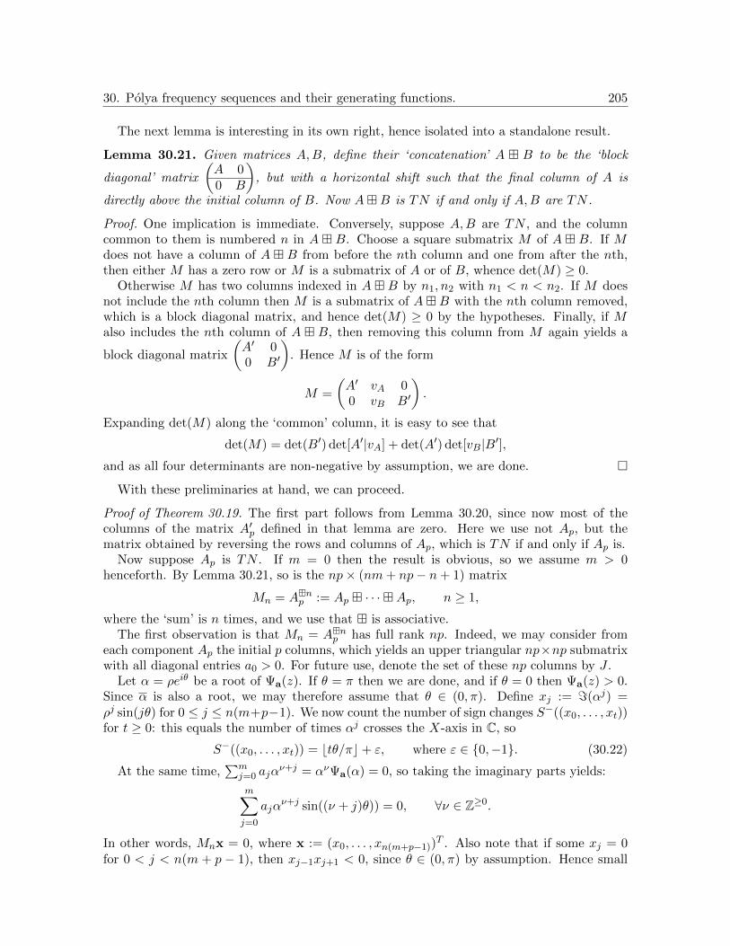
30. Polya frequency sequences and their generating functions. 205

The next lemma is interesting in its own right, hence isolated into a standalone result.

Lemma 30.21. Given matrices A,B, define their ‘concatenation’ A B to be the ‘block

diagonal’ matrix

(A 00 B

), but with a horizontal shift such that the final column of A is

directly above the initial column of B. Now AB is TN if and only if A,B are TN .

Proof. One implication is immediate. Conversely, suppose A,B are TN , and the columncommon to them is numbered n in A B. Choose a square submatrix M of A B. If Mdoes not have a column of A B from before the nth column and one from after the nth,then either M has a zero row or M is a submatrix of A or of B, whence det(M) ≥ 0.

Otherwise M has two columns indexed in A B by n1, n2 with n1 < n < n2. If M doesnot include the nth column then M is a submatrix of AB with the nth column removed,which is a block diagonal matrix, and hence det(M) ≥ 0 by the hypotheses. Finally, if Malso includes the nth column of A B, then removing this column from M again yields a

block diagonal matrix

(A′ 00 B′

). Hence M is of the form

M =

(A′ vA 00 vB B′

).

Expanding det(M) along the ‘common’ column, it is easy to see that

det(M) = det(B′) det[A′|vA] + det(A′) det[vB|B′],and as all four determinants are non-negative by assumption, we are done.

With these preliminaries at hand, we can proceed.

Proof of Theorem 30.19. The first part follows from Lemma 30.20, since now most of thecolumns of the matrix A′p defined in that lemma are zero. Here we use not Ap, but thematrix obtained by reversing the rows and columns of Ap, which is TN if and only if Ap is.

Now suppose Ap is TN . If m = 0 then the result is obvious, so we assume m > 0henceforth. By Lemma 30.21, so is the np× (nm+ np− n+ 1) matrix

Mn = Anp := Ap · · ·Ap, n ≥ 1,

where the ‘sum’ is n times, and we use that is associative.The first observation is that Mn = Anp has full rank np. Indeed, we may consider from

each component Ap the initial p columns, which yields an upper triangular np×np submatrixwith all diagonal entries a0 > 0. For future use, denote the set of these np columns by J .

Let α = ρeiθ be a root of Ψa(z). If θ = π then we are done, and if θ = 0 then Ψa(z) > 0.Since α is also a root, we may therefore assume that θ ∈ (0, π). Define xj := =(αj) =ρj sin(jθ) for 0 ≤ j ≤ n(m+p−1). We now count the number of sign changes S−((x0, . . . , xt))for t ≥ 0: this equals the number of times αj crosses the X-axis in C, so

S−((x0, . . . , xt)) = btθ/πc+ ε, where ε ∈ 0,−1. (30.22)

At the same time,∑m

j=0 ajαν+j = ανΨa(α) = 0, so taking the imaginary parts yields:

m∑j=0

ajαν+j sin((ν + j)θ)) = 0, ∀ν ∈ Z≥0.

In other words, Mnx = 0, where x := (x0, . . . , xn(m+p−1))T . Also note that if some xj = 0

for 0 < j < n(m + p − 1), then xj−1xj+1 < 0, since θ ∈ (0, π) by assumption. Hence small

206 30. Polya frequency sequences and their generating functions.

enough perturbations to x will not change the number of sign-changes except at most at theextremal coordinates.

Now let y := (−1, 1, . . . , (−1)np)T and let x0 := (Mn)−1[np]×Jy, with J ⊂ [nm+ np− n+ 1]

the set of columns chosen above, containing a0. Let x0 ∈ Rnm+np−n+1 \0 denote the vectorwith the coordinates of x0 in the positions indexed by J , and padded by zeros otherwise.Then Mnx0 = y. Now by the end of the preceding paragraph, choose ε > 0 small enoughsuch that S−(x + εx0) ≤ S−(x) + 2. Recalling that Mnx = 0, we have:

np− 1 = S−(εy) = S−(Mn(x + εx0)) ≤ S−(x + εx0) ≤ S−(x) + 2,

where the first inequality is by the variation diminishing property of the TN matrix Mn =Anp (see Theorem 29.11). Hence by (30.22) with t = n(m+ p− 1),

np− 1 ≤ bn(m+ p− 1)θ/πc+ 2 ≤ n(m+ p− 1)θ

π+ 2.

Since n was arbitrary, letting n→∞ finishes the proof.

We can now deduce the desired corollary about finite Polya frequency sequences.

Corollary 30.23. Suppose a = (. . . , 0, a0, . . . , am, 0, . . . ) is a real sequence, with a0, . . . , am >0. The following are equivalent:

(1) a is a Polya frequency sequence.(2) Ψa(x) =

∑mj=0 ajx

j has m negative real roots, counted with multiplicity.

(3) Ψa(x) =∑m

j=0 ajxj has m real roots, counted with multiplicity.

Proof. That (1) =⇒ (2) follows from the final assertion of Theorem 30.19, letting p → ∞.That (2) =⇒ (1) follows from Lemma 30.8. Clearly (2) =⇒ (3), and the converse holdssince Ψa does not vanish at 0, and does not have positive roots by Descartes’ Rule of Signs– see e.g. Theorem 10.7 with I = (0,∞).

30.6. Jacobi TNp matrices and a sufficient condition for TNp sequences. We concludethis section with a result by Schoenberg that is ‘opposite’ to his Theorem 30.19. Namely, ifthe generating polynomial above has no roots in the sector | arg(z) − π| ≤ π/(p + 1), thenthe finite sequence (. . . , 0, a0, . . . , am, 0, . . . ) is TNp. To do so, we first study when ‘infiniteToeplitz tri-diagonal (Jacobi) matrices’ are TNp. This was carried out by Karlin in Trans.Amer. Math. Soc. (1964), and he showed the following lemma.

Lemma 30.24 (Karlin, [199]). Given a, b, c ∈ (0,∞), define the corresponding Jacobi matrixJ(a, b, c)Z×Z via J(a, b, c)j,k equals a, b, c if k = j − 1, j, j + 1 respectively, and 0 otherwise.

Then J(a, b, c) is TNp for an integer p ≥ 1, if and only if b2√ac≥ cos(π/(p+ 1)).

Proof. When considering submatrices of K := J(a, b, c) of the form K[x; y] for x,y ∈ Zr,↑, itis not hard to verify that if xt 6= yt for some 1 ≤ t ≤ r, then (a) the matrix K[x; y] has a rowor a column with at most one non-zero entry; (b) expanding along this row or column breaksup the matrix into the single non-zero entry (if it exists) and a product of two smaller minorsof K = J(a, b, c). From this it follows that every minor of K is a product of principal minorsand elements of K. Thus, to check if J(a, b, c) is TNp, we need to examine the principalminors of size at most p.

For the ensuing discussion, fix a, c > 0. Given λ ∈ C, b ∈ (0,∞), and an integer r ≥ 1,define Jr,b(λ) to be the r × r leading principal submatrix of J(a, b, c)− λ IdZ×Z. Expandingalong an initial/terminal row/column, it is easy to observe that the determinants

dr,b(λ) := detJr,b(λ), r = 1, 2, . . .

30. Polya frequency sequences and their generating functions. 207

are polynomials in λ, which satisfy the recurrence:

dr+1,b(x) = (b− x)dr,b(x)− acdr−1,b(x), r ≥ 0

with the initial conditions d0,b(x) = 1, d−1,b(x) = 0. Reformulate this in terms of the ‘shifted’polynomials

er,b(x) =√ac−rdr,b(b− 2

√acx), r ≥ 1,

to obtain the recurrence:

xer,b(x) =er−1,b(x) + er+1,b(x)

2, r ≥ 1; e0,b(x) = 1, e−1,b(x) = 0.

Restricting to x = λ ∈ (−1, 1), so that x = cos(θ) for some θ ∈ (0, π), one can show byinduction that er(x) = sin((r+ 1)θ)/ sin(θ) satisfies the initial conditions and the recurrence.In fact, this corresponds to the Chebyshev polynomials of the second kind, given by

er(cos θ) =sin(r + 1)θ

sin θ, θ ∈ (0, π), r ≥ −1.

We now fix a, c > 0 and first vary b ∈ (0, 2√ac), so that b

2√ac

= cos(θ) ∈ (0, 1), whence

θ ∈ (0, π/2). Our desired value of interest is the determinant

dr(0) =√acrer,b(b/2

√ac) =

√acrer,b(cos θ) =

√acr sin((r + 1)θ)

sin θ.

This is non-negative if and only if (r+1)θ ≤ π, if and only if 1 > b2√ac≥ cos(π/(r+1)). This

completes the classification if 0 < b < 2√ac, since the sequence cos(π/(r + 1)) is increasing

in 1 ≤ r ≤ p.Returning to our original notation of Jr,b(a, c), note by the multilinearity of the determinant

in the rows/columns that for any square r × r matrix B over a unital commutative ring,

det(B + λ Id) = λr +∑∅6=I⊂[r]

λr−|I| detBI×I . (30.25)

We now apply this fact to the matrices Jr,b(a, c), if b ≥ 2√ac. Set

br := cos(π/(r + 1)), B := Jr,br(a, c), λ :=b

2√ac− br ≥ 0.

Then br > b1, . . . br−1, so detBI×I ≥ 0 from the above analysis. It follows from (30.25) thatdet Jr,b(a, c) ≥ 0. Since this holds for all 1 ≤ r ≤ p, the proof is complete.

With Lemma 30.24 at hand, we present the final proof in this section: that of a sufficientcondition for a polynomial to generate a finite Polya frequency sequence.

Theorem 30.26 (Schoenberg, [325]). Fix an integer p ≥ 1, and suppose a polynomial f(z) =a0z

n + a1zn−1 + · · ·+ an as above, with real coefficients and such that all zeros of f lie in the

sector

| arg(z)− π| ≤ π

p+ 1.

Then the sequence a = (. . . , 0, a0, . . . , an, 0, . . . ) is TNp.

Proof. If p = 1 then the result is clear, so we suppose below that p ≥ 2. Decompose f intolinear and complex-conjugate factors:

f(z) = a0

∏j

(z − αj)∏k

(z − ρke−iθk)(z + ρkeiθk),

208 30. Polya frequency sequences and their generating functions.

with all ρk > 0. The hypotheses imply that αj < 0 and |θk − π| ≤ π/(p + 1). Now z − αjgenerates a PF sequence by Lemma 30.8, and each irreducible quadratic

(z − ρke−iθk)(z + ρkeiθk) = z2 − 2zρk cos(θk) + ρ2

k

does the same by Lemma 30.24, since the condition − cos θk ≥ cosπ/(p+ 1) is equivalent to|θk − π| ≤ π/(p + 1) (with p ≥ 2). Hence their product f(z) also generates a PF sequence,by Proposition 30.6(3).

Finally, we present a (standalone) sufficient condition for a square matrix to be TP :

Theorem 30.27. Let A = (ajk)j,k≥1 with all ajk ∈ (0,∞). If

ajkaj+1,k+1 > aj,k+1ak+1,j · 4 cos2(π/(n+ 1)), ∀j, k ≥ 1,

then A is TPn; moreover, the constant 4 cos2(π/(n+ 1)) cannot be reduced.

This result only uses the positivity of the entries and a growth condition on the 2 × 2minors. It was conjectured by Dimitrov–Pena in 2005 [101], and proved (independently)by Katkova–Vishnyakova in 2006 [209]. (Also worth mentioning is their 2008 follow-up pa-per [210] on (Hurwitz) stability of polynomials.) That the constant is best possible is revealed

via Lemma 30.24, as follows: given 0 ≤ c < 4 cos2(π/(n + 1)), choose θ ∈(

πn+1 ,

2πn+1

)such

that c < 4 cos2 θ. Now consider the Jacobi matrix J(1, 2 cos θ, 1)n×n.

31. Complement: Root-location results and TN Hurwitz matrices. 209

31. Complement: Root-location results and TN Hurwitz matrices

We take a short detour to discuss some well-known matrices associated to finite Polyafrequency sequences and their generating polynomials. First, Corollary 30.23 has receivedrecent attention: instead of working with the matrix Ap as in Theorem 30.19, one can studyother variants. This section opens with a few results along these lines, presented withoutproof.

Definition 31.1. Given a polynomial with real coefficients

f(z) = a0zn + a1z

n−1 + · · ·+ an, n, a0, . . . , an > 0,

and an integer 1 ≤ M ≤ n, define aj := 0 for j < 0 or j > n, and the M th generalizedHurwitz matrix to be the Z× Z matrix HM (f), given by

HM (f)j,k := aMk−j , j, k ∈ Z. (31.2)

We now present five results (without proof, and perhaps not all of them ‘best possible’)in the literature, which are similar to each other, and one of which is the Aissen–Edrei–Schoenberg–Whitney corollary 30.23:

Theorem 31.3. Let n, a0, . . . , an > 0 and define f(z) = a0zn + a1z

n−1 + · · · + an. Also fixan integer 1 ≤M ≤ n.

(1) (M = 2, Routh–Hurwitz, see e.g. [188, 304].) The polynomial f is ‘stable’, i.e., has nozeros z with | arg z| ≤ π/2, if and only if all leading principal minors of the Hurwitzmatrix H2(f), of order ≤ n, are positive.

(2) (M = 2, Asner [14], Kemperman [212], Holtz–Tyaglov [181].) The polynomial f hasno zeros z with | arg z| < π/2 if and only if the Hurwitz matrix H2(f) is TN .

(3) (M = 1, Aissen–Edrei–Schoenberg–Whitney.) The polynomial f has no zeros z with| arg z| < π if and only if the Toeplitz matrix H1(f) is TN .

(4) (M = n, Cowling–Thron [89].) The polynomial f has no zeros z with | arg z| ≤ π/n.(5) (M ∈ [1, n], Holtz–Khrushchev–Kushel [180].) The polynomial f has no roots z with| arg z| < π/M if the generalized Hurwitz matrix HM (f) is TN .

We now come to further results on root-location (of real polynomials), in the spirit ofTheorems 30.19, 30.26, and 31.3. These three results revealed a connection between Polyafrequency sequences, totally non-negative matrices, and root-location.

As a ‘warmup’, we show the Gauss–Lucas theorem, found in Lucas’s 1874 work [244].

Theorem 31.4 (Gauss–Lucas). If p(z) is a non-constant polynomial, then the roots of p′(z)in C are contained in the convex hull of the set of roots of p(z).

Proof. Let p(z) = pn∏nj=1(z−ξj). If ξj is a root of p′ as well as p, then ξj = 1·ξj+

∑k 6=j 0·ξk.

If ξ is a root of p′ but not of p, then we compute:

p′(z)

p(z)=

n∑j=1

1

z − ξj=⇒ 0 =

p′(ξ)

p(ξ)=

n∑j=1

ξ − ξj|ξ − ξj |2

.

Setting A :=∑n

j=1 |ξ − ξj |−2 > 0, we obtain via simplifying and conjugating:

Aξ =

n∑j=1

|ξ − ξj |−2ξj =⇒ ξ =

n∑j=1

|ξ − ξj |−2

Aξj ,

and so ξ is in the convex hull of the ξj .

210 31. Complement: Root-location results and TN Hurwitz matrices.

The next theorem is a ‘real’ variant of the Hermite–Biehler theorem – the classical version isdue to Hermite [165] and Biehler [49] in J. reine angew. Math., in 1856 and 1879 respectively.6

The real variant presented here requires the following preliminary result.

Lemma 31.5. Suppose p, q are differentiable functions on a closed interval [a, b], with p(a) =p(b) = 0, p > 0 on (a, b) and q < 0 on [a, b]. Then there exist λ, µ > 0 such that λp+ µq hasa repeated root in (a, b).

Proof. Since q is continuous and negative on [a, b], define

h(x) :=p(x)

q(x), x ∈ [a, b].

Clearly h is differentiable on [a, b], negative on (a, b), and vanishes at the endpoints. Henceit has a global minimum, say at x0 ∈ (a, b) – whence the function

h(x)− h(x0) : [a, b]→ R

has a repeated root at x0. Returning to p, q, let λ = 1 and µ = −h(x0) > 0; then the function

λp(x) + µq(x) = q(x) (h(x)− h(x0))

can be easily verified to have a repeated root at x0 ∈ (a, b).

We also require the notion of interlacing.

Definition 31.6. Let f, g ∈ R[x] be two real-rooted polynomials, with deg(f)−1 ≤ deg(g) ≤deg(f). We say g interlaces f if between any two consecutive roots of f (possibly equal),there exists a root of g. We say f, g are interlacing, or interlace (one another) if either of f, ginterlaces the other.

For the next few results, and related variants, and an in-depth treatment, the reader isreferred to the monograph [294] of Rahman and Schmeisser. The treatment here is from [179].

Theorem 31.7 (Hermite–Biehler, ‘real’ version). Fix polynomials p, q ∈ R[x] and set f(x) :=p(x2) + xq(x2). The following are equivalent:

(1) The polynomial f(x) has no roots z with <(z) ≥ 0.(2) The polynomials p(−x2), xq(−x2) have real, simple roots, which are interlacing. More-

over, there exists z0 ∈ C, <(z0) > 0 such that <(

p(z20)

z0q(z20)

)> 0.

Proof. We begin by assuming (2). Notice that all roots of p, q lie in (−∞, 0]. Thus the ratio

<(p(z2)zq(z2)

)is non-vanishing, whence always positive by (2), on the half-plane <(z) > 0 (which

is an open ‘sector’ with aperture π; this is defined and used in a later section). It followsthat the equation

0 = f(z) = zq(z2)

(p(z2)

zq(z2)+ 1

)has no solution with <(z) > 0. Moreover, at a point ix on the imaginary line, we have

f(ix) = p(−x2) + ixq(−x2),

which cannot vanish by (2). This shows that all zeros z of f satisfy: <(z) < 0.

6Two historical asides: Biehler’s thesis in the same year 1879 is dedicated to his “master M. CharlesHermite”; and Pierre Fatou was a student of Biehler in the College Stanislas.

31. Complement: Root-location results and TN Hurwitz matrices. 211

Conversely, suppose (1) holds. Write f(z) = a∏mj=1(z − αj), with a 6= 0 and <(αj) < 0.

Verify that if =(z) > 0, then |iz + αj | > |iz − αj | for all j, so that

|f(iz)| = |a|m∏j=1

| − iz + αj | = |a|m∏j=1

|iz + αj | > |a|m∏j=1

|iz − αj | = |f(iz)|.

Square both sides and expand, to deduce using that p(x), q(x) ∈ R[x]:

0 >1

4(|f(iz)|2 − |f(iz)|2) = <(ip(−z2)zq(−z2)) =⇒ =(p(−z2)zq(−z2)) < 0.

This holds if =(z) > 0; taking conjugates, if =(z) < 0 then =(p(−z2)zq(−z2)) > 0. That is:

z 6∈ R =⇒ =(z)=(p(−z2)

zq(−z2)

)< 0. (31.8)

In other words, the functions

z 7→ p(−z2)

zq(−z2), z 7→ zq(−z2)

p(−z2)

do not take real values for z ∈ C\R. Thus, if the first (or second) function here equals −µ/λ(or −λ/µ) for λ, µ ∈ R, then z must be real – that is, the following functions are real-rooted:

λp(−z2) + µzq(−z2), λ, µ ∈ R, λ2 + µ2 6= 0 (31.9)

We next claim that the polynomials p(−x2), xq(−x2) – which are now real-rooted – aremoreover coprime. Suppose not, for contradiction. If p(c) = q(c) = 0 for c ∈ (−∞, 0) then

f(±i√|c|) = 0, which violates (1). If p(0) = 0 then f(0) = 0, again violating (1). Otherwise

p(−x2), xq(−x2) must have a pair of common, non-real conjugate roots, say z± = a± ib withb > 0. Now

f(ia∓ b) = f(iz±) = p(−z2±) + iz±q(−z2

±) = 0,

which violates (1) yet again. This contradiction shows that p(−x2), xq(−x2) are coprime.We now explain why no function (31.9) can have a multiple root. (Recall that these

functions are all real-rooted.) Indeed, if there existed such a multiple root, then one of the

ratio-functions p(−z2)zq(−z2)

, zq(−z2)

p(−z2)– call it g(x) – would equal a real number, say r ∈ R, with

‘multiplicity’. More precisely, there exists x0 ∈ R such that (x − x0)2 divides λp(−x2) +µxq(−x2) with (λ, µ) 6= (0, 0). Notice by the coprimality above that p(−x2), xq(−x2) do notvanish at x0. Let k ≥ 2 denote the order of the multiple root x0. Thus,

g(x)− r = (x− x0)kh(x),

where we expand near x0 and so all functions involved are analytic; moreover, h(x0) 6= 0.But then for small ε > 0, the equation g(x) = r − εk has solutions

x = x0 + eiπ(1+2j)/kh(x0)−1/kε+ o(ε), j = 1, 2, . . . , k.

This implies that the ratio-function g(x) takes real values outside the real axis, which con-tradicts a conclusion above.

We have thus shown that p(−x2), xq(−x2), and indeed, all nontrivial real-linear combina-tions of them, are real-rooted with simple roots. By (the contrapositive of) Lemma 31.5, itfollows that the roots of p(−x2), xq(−x2) interlace. Finally, return to (31.8) and let z := iz0

for arbitrary z0 ∈ (0,∞). Then 0 > =(

p(z20)iz0q(z0)2

)=−p(z20)z0q(z0)2

∈ R.

212 31. Complement: Root-location results and TN Hurwitz matrices.

Remark 31.10. Theorem 31.7(2) is equivalent to the polynomials p, q having simple, nega-tive roots, which interlace with the rightmost zero being that of p, and p(0)q(0) > 0.

As an application, we show the heart of the Routh–Hurwitz scheme [188, 304]. This willpresently lead us back to TN matrices.

Theorem 31.11 (Routh–Hurwitz). Fix polynomials p, q ∈ R[x] and set f(x) := p(x2) +xq(x2). The following are equivalent:

(1) The polynomial f(x) has no roots z with <(z) ≥ 0.(2) The scalar c := p(0)/q(0) is positive and the polynomial f1(x) := p1(x2)+xq1(x2) has

no roots z with <(z) ≥ 0 – where p1(x) := q(x) and q1(x) := 1x(p(x)− cq(x)).

For completeness, we highlight the applicability of the above approach, by deducing anotherwell-known result on interlacing. This is attributed to several authors: Hermite [165] in 1856;Kakeya, whose proof was presented by Fujiwara [133] in 1916; and Obrechkoff [272] in 1963.

Theorem 31.12 (Hermite, Kakeya, Obrechkoff). Suppose f, g are real polynomials with nocommon root. The following are equivalent:

(1) The roots of f, g are real and simple, and f, g interlace (so |deg(f)− deg(g)| ≤ 1).(2) For all λ, µ ∈ R with λ2 +µ2 > 0, the polynomial λf(x)+µg(x) has real, simple roots.

Proof. In both assertions, note that the deg(f) + deg(g) roots of f, g are pairwise distinctand all real, so say f (respectively, g) has roots α1 < · · · < αm (respectively, β1 < · · · < βn).These divide the real line into m+ n+ 1 open intervals, on each of which f, g do not changesign. Enumerate these intervals from right to left, so that I1 = (maxαm, βn,∞). Moreover,on any two adjacent intervals, one of f, g does not change sign, while the other does.

We now turn to the proof. First given (2), we need to show that the polynomials f, ginterlace. (Note that both have real, simple roots.) This follows from the claim that nobounded interval Ik has both endpoints as roots of either f or of g. In turn, the claim is aconsequence of Lemma 31.5.

Conversely, we assume (1) and show (2). We can assume both λ, µ 6= 0, so suppose withoutloss of generality that (a) λ = 1, (b) f, g are monic, and (c) deg(f) = m ≥ n = deg(g), withn ∈ m− 1,m. There are now several cases:

(1) µ > 0. In this case, the function λf + µg is positive on I1, negative on I3, positiveon I5, and so on, until it has sign (−1)m−1 on I2m−1, and (−1)m as x→ −∞. Fromthis, it follows that λf + µg has at least m sign changes on R, and degree m, whenceprecisely m simple roots.

(2) µ < 0 and m = n + 1. In this case, λf + µg is positive as x → +∞, negative on I2,positive on I4, and so on, until it has sign (−1)m on I2m. Now the final sentence ofthe previous case again applies.

(3) −1 < µ < 0 and m = n. Now there are two subcases, corresponding to if αm > βn orαm < βn. In the former case, λf +µg is positive as x→ +∞, negative on I2, positiveon I4, and so on, until it has sign (−1)m (as in the preceding case). Hence the finalsentence of the first case again applies.

Otherwise we have αm < βn, whence λf +µg is positive on I2, negative on I4, andso on, until it has sign (−1)m−1 on I2m, and sign (−1)m as x→ −∞. Hence the finalsentence of the first case applies.

(4) If µ < −1 and m = n, this reduces to the preceding case, by replacing f ←→ g and(λ = 1, µ ∈ (−∞,−1))←→ (µ−1 ∈ (−1, 0), 1).

31. Complement: Root-location results and TN Hurwitz matrices. 213

(5) This leaves the final subcase, in which µ = −1 and m = n (and recall that λ = 1and f, g are monic). Given the interlacing of the roots of f, g, it is not hard to seethat deg(λf + µg) = m − 1. Notice that shifting the origin simultaneously for bothpolynomials does not affect either assertion in the theorem, nor does interchangingλ = 1 with µ = −1. Thus, we assume henceforth that both f and g have negative,simple roots αj and βj respectively, and that without loss of generality,

0 > αm > βm > αm−1 > · · · > α1 > β1.

We now ‘invert the coefficients’ of both polynomials: let finv(x) := xmf(1/x) andginv(x) := xmg(1/x). These have roots α−1

j and β−1j respectively, so these roots

are once again negative and interlacing (now β−11 is the closest root to the origin).

Moreover, finv(0) = ginv(0) = 1. Applying Remark 31.10 (and Theorem 31.7), thepolynomial

F (x) := ginv(x2) + xfinv(x

2)

has no roots z with <(z) ≥ 0. Hence by Theorem 31.11 with c = 1, the polynomialF1(x) := g1(x2) + xf1(x2) has no roots z with <(z) ≥ 0, where

g1(x) = finv(x), f1(x) =1

x(ginv(x)− finv(x)).

Now apply Theorem 31.7 for F1, and Remark 31.10 for g1, f1, to deduce thatthe roots of g1, f1 are simple, negative, and interlace. In particular, the roots of1x(ginv(x)− finv(x)) = (g − f)inv(x) (by abuse of notation) are simple and negative.

Inverting back the coefficients (via p(x) 7→ xdeg(p)p(1/x)), so are the roots of g(x) −f(x), whence of λf + µg, as desired.

32. Examples of Polya frequency functions: Laplace transform, convolution. 215

32. Examples of Polya frequency functions: Laplace transform,convolution.

In Section 28, we saw some characterizations of TNp functions, and also studied the expo-nential decay of TN2 (whence all TNp) functions. We also saw several examples of TN (infact, Polya frequency) functions in Section 29. We now return to Polya frequency functions,and discuss additional examples as well as a recipe to generate new examples of TNp or PFfunctions from old ones.

32.1. The bilateral Laplace transform of a totally non-negative function. We beginby defining and studying the Laplace transform more generally – for TN2 functions.

Definition 32.1. The bilateral Laplace transform of a (measurable) function f : R → R isdenoted by B(f), and defined at a complex argument s ∈ C to be

B(f)(s) :=

∫Re−sxf(x) dx.

This expression is defined if the following integrals both converge as R→∞:∫ R

0e−sxf(x) dx,

∫ 0

−Re−sxf(x) dx,

in which case the sum of their limits is taken to be B(f)(s).

The following result uses the characterization of TN2 functions in Theorem 28.4 above, toshow the existence of the Laplace transform:

Lemma 32.2. Suppose f : R → R is TN2 and not an exponential. Then B(f) exists in theopen vertical strip in C, given by

−∞ ≤ α := infx∈I

(log f)′(x) < β := supx∈I

(log f)′(x) ≤ ∞,

where f ′ exists on a co-countable set, and we set α := −∞ (respectively, β :=∞) if f(x) ≡ 0for sufficiently large x > 0 (respectively, sufficiently small x < 0). If f is integrable then thisstrip contains the imaginary axis.

Proof. Let I denote the interval of support of f , as in Theorem 28.4. There are threepossibilities: (a) I is bounded, in which case the result is easy; (b) I is unbounded only onone side (in which case f can be an exponential function on I); or (c) I = R, in which casef(x) is not an exponential.

We will work in the third case, as the cases for I ( R are simpler. It suffices to show thatthe integral in B(f) is absolutely convergent on a vertical strip. We now appeal to Propo-sition 28.8 and its proof, used henceforth without further reference. First by Lemma 26.3,(log f)′ is defined on a co-countable subset of I and is non-increasing there. Thus the followinglimits make sense, and equal the asserted formulae:

α := limx→∞

f ′(x)

f(x), β := lim

x→−∞

f ′(x)

f(x); (32.3)

moreover, −∞ ≤ α < β ≤ ∞, since f is not an exponential on I = R.We claim that the integral in B(f)(s) is absolutely convergent for <(s) ∈ (α, β), whence

convergent as desired. Indeed:

|B(f)(s)| ≤∫R|e−sx|f(x) dx =

∫ ∞0

e−x<(s)f(x) dx+

∫ 0

−∞e−x<(s)f(x) dx.

216 32. Examples of Polya frequency functions: Laplace transform, convolution.

Since α < <(s) < β, choose points x1 < x2 in I such that α < g′(x2) < <(s) < g′(x1) < β.Then convergence follows because f shrinks to zero faster than the exponential bounds inthe proof of Proposition 28.8.

Finally, suppose f is integrable on I, where we once again assume I = R. Then f(x)→ 0as |x| → ∞, whence log f(x)→ −∞ as |x| → ∞. It follows that α < 0 < β.

We next bring the limits of the vertical strip α, β into the form found in the literature:

Proposition 32.4. The limits in Lemma 32.2 can also be written as

α := limx→∞

log f(x)

x, β := lim

x→−∞

log f(x)

x,

where once again, we set α := −∞ (respectively, β := ∞) if f(x) ≡ 0 for sufficiently largex > 0 (respectively, sufficiently small x < 0).

Proof. The result is nontrivial only for I unbounded on one or both sides of the origin; weshow it here only for the case I = R. Since − log f is convex, the result follows from a moregeneral fact about arbitrary convex functions:

Suppose g : R→ R is convex, so that g′ is defined on a co-countable set. Then,

supx∈R

g′(x) = limx→∞

g′(x) = limx→∞

g(x)

x,

infx∈R

g′(x) = limx→−∞

g′(x) = limx→−∞

g(x)

x.

We only show the first part; the second is similar. By Lemma 26.3(1), the divided difference

h(x, y) :=g(y)− g(x)

y − x, x 6= y

is coordinatewise non-decreasing. Choose any x0 at which g is differentiable. Then for y > x0,

h(x0, y) ≥ limy→x+0

h(x0, y) = g′(x0);

but now taking y →∞,

g′(x0) ≤ limy→∞

g(y)− g(x0)

y − x0= lim

y→∞

g(y)

y.

Taking the supremum over x0 ∈ R (or the limit as x0 → ∞) yields one inequality. For theother, let g be differentiable at x0 and let y < x0. Then

h(y, x0) ≤ limy→x−0

h(y, x0) = g′(x0) ≤ supx∈R

g′(x).

Since this holds for all x0 > y, now taking x0 →∞ yields the desired result:

supx∈R

g′(x) ≥ limx0→∞

g(x0)− g(y)

x0 − y= lim

x0→∞

g(x0)

x0.

32.2. Examples of Polya frequency functions; convolution. Having discussed theLaplace transform, we next discuss a recipe to generate new examples of TNp functions(or Polya frequency functions) from old ones, for all p ≥ 1.

Definition 32.5. Given Lebesgue measurable functions f, g : R → R, define their convolu-tion, denoted by f ∗ g, to be the function given by the following integral, wherever defined:

(f ∗ g)(x) :=

∫Rf(y)g(x− y) dy.

32. Examples of Polya frequency functions: Laplace transform, convolution. 217

The recipe can now be stated: if f, g are integrable TNp functions for any 1 ≤ p ≤ ∞,then so is f ∗ g. To show this, we require some basic properties of convolutions, which arenow collected together for ease of future reference.

Lemma 32.6 (Convolution properties). Suppose f, g : R→ R are both in L1(R).

(1) For almost all x ∈ R, the function y 7→ f(y)g(x − y) is Lebesgue measurable andintegrable, so that f ∗ g is defined for almost every x ∈ R.

(2) f ∗ g = g ∗ f ∈ L1(R), and ‖f ∗ g‖1 ≤ ‖f‖1‖g‖1.(3) If g is also in L∞(R), then f ∗ g is continuous on R.(4) If f, g ≥ 0 on R, then so is f ∗ g.(5) The Laplace transform is an ‘algebra homomorphism’ for addition and convolution:

B(f ∗ g)(s) = B(f)(s)B(g)(s),

whenever the two terms on the right converge absolutely at a common point s ∈ R.

Regarding the last part, we leave to the reader the verification that L1(R) under additionand convolution forms a commutative R-algebra.

Proof.

(1) First note that A(x, y) := f(x)g(y) is Lebesgue measurable, since f, g are. Moreover,L(x, y) := (y, x− y) is an invertible linear transformation of R2, whence measurable.Thus (A L)(x, y) := f(y)g(x− y) is measurable. But now A L is also integrable:∫∫

R2

|(A L)(x, y)| dx dy =

∫R

(∫R|g(x− y)| dx

)|f(y)| dy = ‖g‖1‖f‖1 <∞.

Hence the assertion follows by Fubini’s theorem.(2) This is now straightforward:

‖f ∗ g‖1 =

∫R|(f ∗ g)(x)| dx ≤

∫∫R2

|g(x− y)f(y)| dx dy,

and as in the preceding part, the right-hand side equals ‖g‖1‖f‖1. That (f ∗ g)(x) =(g ∗ f)(x) follows by substituting y 7→ x − y in the (improper) integral defining theconvolution.

(3) Suppose xn → x in R as n→∞. Then

|(f ∗ g)(xn)− (f ∗ g)(x)| ≤∫R|f(xn − y)− f(x− y)||g(y)| dy ≤ ‖τhnf − f‖1‖g‖∞, (32.7)

where hn is a real sequence going to 0, and (τhf)(y) := f(y+h) for y, h ∈ R is the shiftoperator. Now recall via Urysohn’s lemma and properties of the Lebesgue measurethat the space of compactly supported functions Cc(R) is dense in (L1(R), ‖ · ‖1).Thus, let fk ∈ Cc(R) converge to f as k →∞; then by the triangle inequality,

‖τhnf − f‖1 ≤ ‖τhnf − τhnfk‖1 + ‖τhnfk − fk‖1 + ‖fk − f‖1. (32.8)

The first and third terms on the right agree, since the Lebesgue measure is translation-invariant. Thus, to show the left side of (32.7) goes to zero as n → ∞, it suffices toshow that the right side of (32.8) goes to zero. For this, fix ε > 0, then fix k 0 suchthat ‖fk − f‖1 < ε/3. Suppose fk is supported on [−ρ, ρ] for 0 < ρ < ∞. Choosen0 0 such that |hn| < ρ for n ≥ n0; then τhnfk − fk is continuous and supportedon J := [−2ρ, 2ρ]. Since fk is uniformly continuous on J , there exists δ > 0 such that

x, y ∈ J, |x− y| < δ =⇒ |fk(x)− fk(y)| < ε

9ρ.

218 32. Examples of Polya frequency functions: Laplace transform, convolution.

Now choose n1 > n0 such that |hn| < min(ρ, δ) for n ≥ n1. Then τhnfk and fkdisagree at most on the interval [−2ρ, ρ] if hn ≥ 0, and on [−ρ, 2ρ] if hn ≤ 0. Hence

‖τhnfk − fk‖1 =

∫R|fk(y + hn)− fk(y)| dy ≤ 3ρ · ε

9ρ=ε

3

for all n ≥ n1. Using (32.8), it thus follows for each ε > 0 that ‖τhnf − f‖1 < ε forall sufficiently large n. This shows continuity on R, by (32.7).

(4) This is immediate from the definition of f ∗ g.(5) We compute:

B(f)(s)B(g)(s) =

∫Rf(y) dy

∫Re−s(y+u)g(u) du =

∫Rf(y) dy

∫Re−sxg(x− y) dx

=

∫Re−sx

(∫Rf(y)g(x− y) dy

)dx =

∫Re−sx(f ∗ g)(x) dx = B(f ∗ g)(s),

where f ∗ g is defined almost everywhere from above. The interchange of integrals inthe first equality on the second line is justified by Fubini’s theorem – which applieshere because∫∫

R2

|f(y)e−sxg(x− y)| dy dx =

∫Re−sy|f(y)| dy ·

∫Re−su|g(u)| du,

and both integrals are finite by assumption.

As an immediate consequence, the above recipe follows:

Corollary 32.9. Suppose f, g : R→ R are integrable TNp functions for some p ≥ 1 (or bothTN functions). Then so is f ∗ g.

Proof. That f ∗ g is integrable follows from Lemma 32.6. That it is TNp follows from theBasic Composition Formula (see (5.14)) and Corollary 6.1.

Two applications of this corollary will be provided presently.Having studied the Laplace transform and convolution, we now come to additional exam-

ples of TN and Polya frequency functions.

Example 32.10. The Heaviside function H1(x) := 1x≥0 is TN . This can be shown usingdirect computations, see e.g. Chapters 1, 3 of Karlin’s book [200], where it is shown that the‘transpose’ kernel K(x, y) = 1x≤y satisfies:

detK[x; y] = 1(x1 ≤ y1 < x2 ≤ y2 < · · · < xp ≤ yp),

for all integers p ≥ 1 and tuples x,y ∈ Rp,↑.

Example 32.11. We are now interested in convolving the previous example with itself severaltimes. However, the function H1 is not integrable. Thus, first use Lemma 28.3 to define

λ1(x) := e−xH1(x) = 1x≥0e−x.

Note, this is an integrable TN function on R, which is discontinuous at the origin. We now

claim that the n-fold convolution fn of λ1 with itself is the function xn−1

(n−1)!λ1(x), for all n ≥ 1.

The verification is by induction on n ≥ 1, with the base case immediate. To show theinduction step, use that fn(x) := xn−1λ1(x)/(n− 1)!, and compute:

fn+1(x) =

∫Rfn(y)f1(x− y) dy.

32. Examples of Polya frequency functions: Laplace transform, convolution. 219

By the induction hypothesis, the integrand vanishes unless y, x − y are both non-negative,whence so is x. Thus fn+1(x) = 0 for x < 0, and for x ≥ 0, we compute:

fn+1(x) =

∫ x

0fn(y)f1(x− y) dy =

∫ x

0

yn−1

(n− 1)!e−y · e−(x−y) dy = e−x

xn

n!.

In particular, xnλ1(x) is an integrable TN function, by Corollary 32.9. Similar to the Gauss-ian, we record the Laplace transform of these functions, for future use. More generally, givena non-negative power α ≥ 0 and a scalar β > 0, let gα,β(x) := xαλ1(βx). Then,

B(gα,β) =

∫ ∞0

e−xsxαe−βx dx =

∫ ∞0

e−x(s+β)xα dx =Γ(α+ 1)

(s+ β)α+1, s > −β. (32.12)

These examples will play a role below, in classifying the total-positivity preservers onarbitrary domains. For now we present a final example, again obtained via convolution:

Example 32.13. Let f(x) := λ1(x) and g(x) := λ1(−x). As these are integrable TN

functions, so is their convolution, which one verifies is e−|x|/2. Hence e(α−β)|x|/2 is TN for

all α < β. Multiplying by e(α+β)x/2, it follows by Lemma 28.3 that the function

f(x) =

ceβ(x−x0), if x ≤ x0,

ceα(x−x0), if x > x0(32.14)

is TN for c ≥ 0 and x0 ∈ R – and integrable when α < 0 < β, as above. Notice also thatthe limiting cases of α = −∞, β = +∞ (both leading to f vanishing on a semi-axis), areintegrable TN functions; while if α = β then f is an exponential, whence also TN .

32.3. Polya frequency functions and the Laguerre–Polya class. It is rewarding toplace the theory of Polya frequency functions (and more generally, TN functions) in itshistorical context before proceeding further. Begin with a scalar δ ≥ 0 and a summablepositive sequence:

αj > 0, j = 1, 2, . . . ,∑j≥1

αj <∞,

so that the terms 1/αj are bounded below by a positive number. Then the convolution

fn(x) := (ϕα1 ∗ · · · ∗ ϕαn)(x), ϕa(x) :=1

aλ1(x/a)

is a Polya frequency function with Laplace transform∏nj=1(1 +αjs)

−1. Given δ ≥ 0, the PF

function Λn(x) := fn(x− δ) therefore satisfies:

B(Λn)(s) = Φ∗n(s), ∀n ≥ 1, <(s) > maxj≤n

(−1/αj), where Φ∗n(s) :=e−δs∏n

j=1(1 + αjs).

Notice for n ≥ 2 that the Φ∗n are dominated uniformly on the imaginary axis by an integrablefunction:

|Φ∗n(ix)| ≤ 1

|(1 + α1ix)(1 + α2ix)|, ∀x ∈ R, n ≥ 2. (32.15)

Hence for n ≥ 2, the Laplace inversion formula recovers Λn from Φ∗n via the Fourier–Mellinintegral, which converges absolutely:

Λn(x) =1

2πilimT→∞

∫ iT

−iTesxΦ∗n(s) ds, ∀x ∈ R.

220 32. Examples of Polya frequency functions: Laplace transform, convolution.

Now since∑

j≥1 αj <∞, we have the convergence of the functions

Φ∗n(s)→ Φ∗(s) :=e−δs∏∞

j=1(1 + αjs),

where the infinite product in Φ∗(s) is defined in the vertical strip maxj(−1/αj) < <(s) <∞,and converges there since

∞∏j=1

|1 + αjs| ≤∞∏j=1

(1 + αj |s|) ≤ exp∞∑j=1

(αj |s|) <∞.

Hence by Lebesgue’s dominated convergence theorem, the integrals Λn also converge to afunction:

limn→∞

Λn(x) = limn→∞

1

2πilimT→∞

∫ iT

−iTesxΦ∗n(s) ds =

1

2πilimT→∞

∫ iT

−iTesxΦ∗(s) ds,

and this holds for all real x. Denote the function on the right by Λ(x); then one can show thatΛ is also a Polya frequency function, which vanishes on (−∞, 0) and is such that B(Λ)(s) =Φ∗(s) for <(s) > maxj(−1/αj). Moreover, the reciprocal of this bilateral Laplace transformis the restriction to the strip <(s) > maxj(−1/αj) of an entire function with only (real)negative zeros:

1

B(Λ)(s)=

1

Φ∗(s)= eδs

∞∏j=1

(1 + αjs). (32.16)

A similar phenomenon occurs when one considers Polya frequency functions that neednot vanish on a semi-axis. In this case one can convolve functions of the form ϕa(±x) for0 6= a ∈ R, as well as the Gaussian kernel (and shifted variants of these). Further takinglimits produces Polya frequency functions whose Laplace transforms are of the form

Φ∗(s) =eγs

2−δs∏∞j=1(1 + αjs)e−αjs

, (32.17)

where

γ ∈ [0,∞), αj , δ ∈ R, 0 < γ +∑j

α2j <∞, max

αj>0(−1/αj) < <(s) < min

αj<0(−1/αj).

Schoenberg showed in J. d’Analyse Math. (1951) the following remarkable result: the abovetoy examples (32.16) and (32.17) (created by convolving variants of λ1 and the Gaussian)are in fact representative of all Polya frequency (PF) functions Λ satisfying

∫R Λ(x) dx = 1 –

with the first toy example a prototype for all PF functions that vanish on (−∞, 0). E.g. thePF functions Λ as in (32.16) are characterized by the fact that 1

B(Λ)(s) is (the restriction to

a vertical strip, of) an entire function ceδs∏∞j=1(1 + αjs), where c ∈ (0,∞), δ, αj ≥ 0, and∑

j αj <∞.In fact, such entire functions were the subject of a beautiful theory built up around the

turn of the 20th century, by experts before Schoenberg – including Laguerre, Polya, andSchur. In the next section, we provide a brief detour into this rich area, before returning toits connections to Polya frequency functions and TN functions.

33. History – The Laguerre–Polya–Schur program:multiplier sequences and entire functions. Modern results. 221

33. History – The Laguerre–Polya–Schur program: multiplier sequences andentire functions. Modern results.

This section undertakes a brief historical journey through one of the most longstandingand mathematically active areas in analysis, with a rich history as well as modern activity:the study of the zeros of (complex) polynomials and entire functions. We already saw someclassical results in Section 31; here we see more such results, now from the viewpoint of linearoperators on polynomial spaces that preserve real-rootedness and similar properties.

The study of roots of complex polynomials has always attracted tremendous attention. Toname two dozen experts with related work before 1930: Descartes (1637); Budan, Gauss,Fourier, Sturm, Cauchy (1800–1840); Chebyshev, Hermite, Poulain, Weierstrass, Routh,Biehler, Lucas (1840–1880); Laguerre, Hadamard, Malo, Markov, Hurwitz, Grace, Van Vleck(1880–1910); Fekete, Kakeya, Polya, Jensen, Schur, Cohn, Szego, Walsh, Obrechkoff (1910–1930). For these and many other classical contributions, see e.g. the 1929 survey [350] byVan Vleck in Bull. Amer. Math. Soc. In the subsequent nine decades, activity in this areahas continued, including papers, surveys, and books; in this section, we briefly allude to theworks [91, 92] by Craven–Csordas (and Smith) and the classic text of Levin [235]. (See themonograph [294] by Rahman–Schmeisser for more on this area.) The section concludes byalluding to a few important contributions to this area, all taken from this millennium.

We begin with notation.

Definition 33.1.

(1) Given a region S ⊂ C, let π(S) denote the class of polynomials with all zeros in S,and coefficients in R (sometimes this is replaced by C). Given an integer n ≥ 1, letπn(S) ⊂ π(S) denote the subset of polynomials with degree at most n.

(2) Given a complex polynomial p, let Znr(p) denote the number of non-real roots of p.

A question that has interested analysts for more than a century is to understand operations– even linear ones – under which πn(S) is stable. This is an old question for which notmany nontrivial answers were known – especially until 2004; see the discussion precedingTheorem 33.40 below. Certainly, some easy answers have long been known. For example, ifp(x) ∈ π(C) = R[x] is real-rooted, then so are:

(1) its product p(x)q(x) with a real-rooted polynomial q(x).(2) the ‘shift’ ap(bx+ c) for scalars a, b, c ∈ R, a 6= 0.(3) the derivative p′(x) – this is Rolle’s theorem. Notice, the derivative operator com-

mutes with all additive shifts/translations.(4) ‘multiplicative differentiation’ xp′(x), again by Rolle’s theorem. In contrast to the

preceding operation, this operator commutes with all multiplicative shifts/dilations.

(5) the ‘inversion’ xdeg(p)p(1/x), whose roots are 0 if p(0) = 0, and x0 6= 0 if p(1/x0) = 0.

All but the first of these operations also are answers to the more general question, ofunderstanding linear transformations on πn(C) that do not increase the number of non-real roots Znr(·). In particular, they answer our first question, of understanding linearoperators preserving real-rootedness. A related, second question involves understandingwhich (linear) operations T preserve real-rootedness, now only on real polynomials with allnon-positive roots (or all non-negative roots). Notice that the operations above are also(positive) examples of such linear operations (e.g. assuming q(x) also has one-sided roots).

Often, one assumes a further restriction on the linear map T in order to have more structureto work with. Two such conditions are that T commutes with the usual/additive derivative

22233. History – The Laguerre–Polya–Schur program:

multiplier sequences and entire functions. Modern results.

∂, or with the multiplicative derivative x∂. Clearly, the latter operators are of the form

T (xk) = γkxk, γ0, γ1, · · · ∈ R

(or γk ∈ C if one considers the analogous problem). Similarly, one can show that the formeroperators each have a ‘power series expansion’

T =

∞∑k=0

T (k)∂k, T (k) ∈ R.

Notice here that applying such an operator to a polynomial only requires finitely many terms,

so the sequence T (k) can be arbitrary. One associates to this operator its symbol :

GT (s) :=∞∑k=0

T (k)sk. (33.2)

In this section we present the characterizations of both classes of operators – commutingwith additive and multiplicative differentiation ∂, x∂ respectively – and they both bear thename of Polya (with Benz and Schur, respectively). We will mostly focus on the latter case,in which the scalars γk are called multipliers. Thus, the Polya–Schur theorem classifies allmultiplier sequences (which preserve real-rooted polynomials).

For now, we return to the opening discussion of preserving real-rootedness, or more gen-erally, diminishing the number of non-real roots. Our journey begins with a classical resultdue to Poulain [292] in 1867, answering a question of Hermite [166] from the previous year:

Theorem 33.3 (Hermite–Poulain). Suppose q(x) =∑m

k=0 qkxk is a polynomial with q0, qm 6=

0 and all real roots.

(1) If p(x) ∈ R[x], then Znr(q(∂)p) ≤ Znr(p); here the differential operator q(∂) acts via

(q(∂)p)(x) :=

m∑k=0

qkp(k)(x).

(2) If q has only positive (respectively, negative) zeros, and A ∈ R, then the number ofzeros in [A,∞) (respectively, (−∞, A]) of q(∂)p exceeds that of q.

Thus, the Hermite–Poulain theorem extends Rolle’s theorem – i.e., that differentiationdiminishes the number of non-real roots of a polynomial – which is the special case q(x) = x.

Proof. To show (1), write q(x) = qm∏j(x − αj), where no αj is zero since q0 6= 0. Since

q(∂) = qm∏j(∂ − αj), it suffices to show that (∂ − α)p(x) has at least as many real roots as

p. We now present Poulain’s proof of this, in a sense ‘differential-equation theoretic’: since

(∂ − α)p(x) = eαx∂(e−αxp(x)),

it suffices to show p(x) has at most as many real roots as (e−αxp(x))′, where α 6= 0. Thisfollows by Rolle’s theorem, since e−αxp(x) vanishes at the roots of p as well as αx → ∞.(This is the trick that was used in proving the weak and strong versions of Descartes’ rule ofsigns, in Lemma 5.2 and Theorem 10.3, respectively.)

This shows the first part, but also the second: the preceding sentence suggests how toproceed if all roots of q are non-zero, with a common sign. Indeed, a small refinement of thepreceding proof now works on [A,∞) (respectively, (−∞, A]).

Notice that the operator q(∂) commutes with ‘additive’ differentiation ∂, a notion discussedabove – and it preserves real-rootedness. A complete characterization of such linear preserverswas carried out by Benz, in Comment. Math. Helv. in 1934:

33. History – The Laguerre–Polya–Schur program:multiplier sequences and entire functions. Modern results. 223

Theorem 33.4 (Polya–Benz theorem, [34]). Suppose T is a linear operator on the spaceof complex polynomials, which commutes with differentiation ∂. Then T preserves real-

rootedness if and only if its symbol GT (s) :=∑∞

k=0 T (k)sk, defined in (33.2), is an entirefunction that is either zero or in the Laguerre–Polya class LP2 (see Definition 33.20):

GT (s) = Csme−γs2+δs

∞∏j=1

(1+αjs)e−αjs, with C ∈ C×;m ∈ Z≥0; γ ≥ 0; δ, αj ∈ R;

∞∑j=1

α2j <∞.

33.1. Multiplier sequences and early results. In the remainder of this section, we focuson the linear transformations which preserve real-rootedness, commute with ‘multiplicativedifferentiation’ x∂, and turn out to be intimately linked to our main objects of focus: Polyafrequency functions. These are the so-called ‘diagonal transforms’ of π(C) – i.e., multiplyingeach monomial xk in a polynomial p(x) by a scalar γk ∈ R. They are called multipliers;corresponding to the two related questions after Definition 33.1, they come in two varieties:

Definition 33.5 (Polya–Schur, [287]). Given a sequence Γ = (γk)∞k=0 of real numbers, define

the linear map Γ[−] : R[[x]]→ R[[x]] (in particular, acting on polynomials) via

Γ

∑k≥0

akxk

:=∑k≥0

γkakxk.

We now say that a sequence Γ is a multiplier sequence of the first kind if Γ[p] is real-rootedwhenever the polynomial p(x) is; and of the second kind if Γ[p] is real-rooted whenever thepolynomial p(x) has all roots real, non-zero, and of the same sign.

Example 33.6 (Laguerre, 1884). Given a real number a > 0 and an integer k > 0, thesequence

a(a+ 1) · · · (a+ k − 1), (a+ 1)(a+ 2) · · · (a+ k), . . .

is a multiplier sequence which preserves the real-rootedness/one-sidedness of roots – and moregenerally, diminishes the number of non-real roots. This follows from a more general result byLaguerre – see Theorem 33.8(2), specialized here to q(x) = (x+a)(x+a+1) · · · (x+a+k−1).

In their famous 1914 work [287] in J. reine angew. Math., Polya and Schur provided‘algebraic’ and ‘transcendental’ characterizations of the above two classes of multipliers; theseare explained below. That said, the study of such multipliers had begun well before. Wepresent here a quintet of well-known results in this direction – these are shown presently:

• by Laguerre, in 1882 in C. R. Acad. and in 1884 in Acta Math.;• by Malo in 1895 in J. Math. Spec. (this is briefly used in the next part of the text);• by Jensen in 1913 in Acta Math.; and• by Schur in 1914, in J. reine angew. Math.

To state and prove these, define the Schur composition of two polynomials/power series:

p(x) =∑j≥0

pjxj , q(x) =

∑j≥0

qjxj , =⇒ (p q)(x) :=

∑j≥0

j!pjqjxj . (33.7)

Theorem 33.8. Suppose p(x) = p0 + p1x+ · · ·+ pnxn and q(x) = q0 + q1x+ · · ·+ qmx

m arepolynomials in R[x], with m,n ≥ 0 and q real-rooted.

(1) (Laguerre [228], 1882.) The polynomial∑

k≥0(qk/k!)xk is real-rooted. In other words,

1, 1, 1/2!, 1/3!, . . . is a multiplier sequence of the first kind.

22433. History – The Laguerre–Polya–Schur program:

multiplier sequences and entire functions. Modern results.

(2) (Laguerre [230], 1884.) Suppose q 6= 0 on [0, n]. Then the polynomial

q(x) := q(0)p0 + q(1)p1x+ · · ·+ q(n)pnxn

has at least as many real roots as p, that is, Znr(q) ≤ Znr(p).(3) (Malo [248], 1895.) Suppose the roots of q are all non-zero and of the same sign. If

p is real-rooted, so is the Hadamard composition p0q0 + p1q1x+ · · ·+ plqlxl (provided

it is not identically zero), where l = minm,n.(4) (Jensen [194], 1913.) The following is a multiplier sequence of the first kind for n ≥ 1:

1, 1, 1− 1

n, (1− 1

n)(1− 2

n), . . . ,

n−1∏j=1

(1− j

n), 0, 0, . . .

(5) (Schur composition theorem [329], 1914.) Suppose the roots of q are all non-zeroand of the same sign. If p is real-rooted, so is the Schur composition p q (or elsep q ≡ 0).

Thus, parts (3) and (5) yield ‘finite’ multiplier sequences of the first kind.

To show these results, we first present a more general theorem, shown in 1949 by de Bruijn:

Theorem 33.9 (de Bruijn, [73]). For an aperture 0 ≤ α ≤ π, let Sα denote an open sectorin the complex plane, given by

Sα := z ∈ C× : arg(z) ∈ (θα, θα + α) (33.10)

for a fixed ‘initial angle’ θα. Similarly, let Sβ denote an open sector for β ∈ [0, π] and

fixed initial angle θβ. Now suppose p(z) =∑n

k=0 pkzk and q(z) =

∑mk=0 qkz

k are complexpolynomials, with pn, qm 6= 0. If p(z), q(z) have all roots in the sectors Sα, Sβ respectively,then their Schur composition p q has all roots in the open sector

−SαSβ := −z1z2 ∈ C : z1 ∈ Sα, z2 ∈ Sβ.

Proof. First suppose (p q)(z) = 0 for some z 6∈ −SαSβ. For any such z, (by abuse ofnotation) −zS−1

α is then disjoint from Sβ, so we can embed both of these in open half-planes(i.e. open sectors of aperture π) −zS−1

α ⊂ S1 and Sβ ⊂ S2 such that S1∩S2 = ∅. In particular,it suffices to show the result for α = β = π. Now for a second reduction: the polynomials

p1(z) := p(−izeiθα) =n∑j=0

p1,jzj , q1(z) := q(−izeiθβ ) =

m∑j=0

q1,jzj ,

can be verified to have all of their roots in the left half-plane in C, i.e., in

L := z ∈ C : <(z) < 0. (33.11)

Hence in this ‘reduction’ case, if we show the following claim – that the polynomial

(p1 q1)(z) := (p q)(−zei(θα+θβ))

has no roots in (0,∞) – then (p q)(z) has no roots in −SαSβ, as desired.While this claim can be shown using Grace’s Apolarity Theorem (see e.g. [365]), we mention

de Bruijn’s direct argument. First claim that if λ ∈ (0,∞), η ∈ L, and P (z) is any non-zeropolynomial with degree n ≥ 0, leading coefficient Pn 6= 0, and all roots in L, then (λ∂ − η)Pis not identically zero and its roots still lie in L. Indeed, write P (z) = Pn

∏nj=1(z − ξj); then

(λ∂ − η)P (z) = P (z)

n∑j=1

λ

z − ξj− η

, ∀z ∈ C \ L.

33. History – The Laguerre–Polya–Schur program:multiplier sequences and entire functions. Modern results. 225

The first factor on the right is non-zero by assumption, while each summand and −η bothhave positive real part, so that the second factor on the right is in −L. It follows that thenon-zero polynomial (λ∂ − η)P (z) again has all roots in L. Now start with

P (z) = p1(z) = p1,n

n∏j=1

(z − ξj), q1(z) = q1,m

m∏j=1

(z − ηj),

and apply the above reasoning inductively for each η = ηj , to conclude that

(q1(λ∂)p1)(z) = q1,0p1(z) + q1,1λp′1(z) + · · ·+ qnλ

np(n)1 (z)

has all its roots in L. In particular, it does not vanish at 0, so

0 6= q1,0p1,0 + 1!q1,1p1,1λ+ · · ·+ l!q1,lp1,lλl, l = minm,n.

This precisely says 0 6= (p1 q1)(λ); as λ ∈ (0,∞) was arbitrary, the proof is complete.

This result led de Bruijn to derive a host of corollaries, which we discuss before returningto the proof of Theorem 33.8. The first is the ‘closed’ sector version of Theorem 33.9:

Corollary 33.12 (de Bruijn, [73]). Suppose p, q 6= 0 are complex polynomials, whose rootsall lie in closed sectors Sα, Sβ respectively. If both α, β ∈ [0, π], then either p q ≡ 0 or it

has all roots in the sector −Sα Sβ. (If an aperture is 0, that closed sector is a half-line.)

Proof. This is obtained from Theorem 33.9 via limiting arguments (and the continuity ofroots, e.g. by Hurwitz’s theorem), when the apertures of both sectors are positive. If eitheraperture is zero, write the corresponding half-line as an intersection of a sequence of nestedclosed sectors with positive apertures, and apply Corollary 33.12 for each of these.

The next corollary shows two results of Weisner, from his 1942 paper in Amer. J. Math.:

Corollary 33.13 (Weisner, [365, Theorem 1 and its Corollary]). Suppose p, q are polynomialsin R[x] with q(x) having all real roots.

(1) If the roots of p(x) lie in a closed sector Sα with aperture ≤ π, then either p q ≡ 0or it has all roots in the ‘double sector’ ±Sα.

(2) If the roots of q are moreover negative, and a closed sector with aperture in [0, π]contains the roots of p, it also contains the roots of p q.

Proof. For the first part: if p q ≡ 0 or Sα has aperture π then the result is immediate; nowsuppose neither condition holds. Apply Corollary 33.12 twice: with Sβ the lower and upperhalf-planes ±iL, where L is the left half-plane (33.11). It follows that the roots of p q lie in

(−iL · Sα) ∩ (iL · Sα) = Sα ∪ −Sα.This shows the first part; for the second, apply Corollary 33.12 with Sβ = (−∞, 0].

The next corollary is a mild strengthening of another result by de Bruijn [73]; his proofworks for the following as well.

Corollary 33.14 (de Bruijn, [73]). Fix scalars −∞ < δ < 0 ≤ ∆ ≤ +∞, and suppose thepolynomials p, q ∈ C[z]\0 both have all roots in the strip =(z) ≥ −∆. Then the polynomial

ϕδ(z) :=

∞∑k=0

δk

k!p(k)(z)q(k)(z)

has all roots also in the same strip =(z) ≥ −∆.

22633. History – The Laguerre–Polya–Schur program:

multiplier sequences and entire functions. Modern results.

Notice that ϕδ(z) has the same form as the Schur composition, but in the ‘other’ parameter.Namely, ϕz(0) = (p q)(z). This is used in the proof.

Proof. Fix a non-real number w with =(w) < −∆. We need to show that ϕδ(w) 6= 0. To doso, consider the polynomials

P (z) :=

∞∑k=0

zkp(k)(w)

k!= p(z + w), Q(z) :=

∞∑k=0

zkq(k)(w)

k!= q(z + w).

By assumption, the zeros z of P,Q lie in the upper half-plane, which is an open sectorwith aperture π. Hence by Theorem 33.9, the roots z (not w) of their Schur compositionϕz(w) = (P Q)(z) all lie in C \ (−∞, 0]. In particular, ϕδ(w) = (P Q)(δ) 6= 0, by choiceof δ.

Remark 33.15. If instead p, q have all roots in the strip =(z) ≤ ∆, a similar argument showsthat so does ϕδ. Intersecting these two results yields the version in de Bruijn’s paper [73], i.e.,for the strip |=(z)| ≤ ∆. In particular, if ∆ = 0, this also shows that if p, q are real-rooted,then so is ϕδ. However, the above approach has the advantage that de Bruijn’s results alsoyield root-location results in asymmetric strips =(Z) ∈ [−∆,∆′] for 0 ≤ ∆ 6= ∆′.

Finally, we prove the classical results stated above.

Proof of Theorem 33.8. We show the five parts in a non-sequential fashion, beginning withpart (2) by Laguerre. It turns out this is precisely the counterpart of the Hermite–Poulaintheorem 33.3, now for the ‘multiplicative differential’ operator x∂ instead of the usual deriv-ative ∂. Indeed, write q(x) = qm

∏mj=1(x−αj) with αj ∈ R, and compute at each monomial:

q(x∂)(xk) = qm

m∏j=1

(x∂ − αj)(xk) = xk · qmm∏j=1

(k − αj) = q(k)xk.

Since the factors (x∂ − αj) pairwise commute, it again suffices to show (x∂ − α)p(x) has atleast as many real roots as p, if α ∈ R \ [0,deg(p)] (so we may assume deg(p) = n). Wenow study the order of the root at 0, and the positive/negative roots of both polynomials pand (x∂ − α)p. The orders of the root at zero agree. Coming to positive roots, write usingPoulain’s idea:

(x∂ − α)p(x) = xα+1∂(x−αp(x)).

Now if α < 0 then x−αp(x) has an additional zero at x = 0; while if α > n, x−αp(x) has anadditional ‘zero’ at x = +∞. In both cases, one argues as in the proof of the Hermite–Poulaintheorem 33.3 above, using Rolle’s theorem to obtain that the positive roots of (x∂ − α)p(x)are at least as many as that of p(x) – if x > 0. A similar argument holds for x < 0.

Next, part (5), i.e., the Schur composition theorem, is a special case of Corollary 33.13(1),in which the roles of p and q are reversed, and one takes Sα to be a closed semi-axis in R.To now obtain the result of Laguerre (part (1)), first apply ‘inversion’ to observe that if

q(x) = q0 + q1x+ · · ·+ qmxm

is real-rooted, then so is its ‘inversion’ (possibly up to a power of x),

Q(x) := qm + qm−1x+ · · ·+ q0xm.

Now let P (x) := (1 + x)m; then by part (5) the polynomial

(P Q)(x) = qm + qm−1m!

(m− 1)!x+ qm−2

m!

(m− 2)!x2 + · · ·+ q0m!xm

33. History – The Laguerre–Polya–Schur program:multiplier sequences and entire functions. Modern results. 227

is also real-rooted. Again invert this (and multiply by powers of x if necessary), and thendivide throughout by m! to obtain Laguerre’s result, i.e., part (1).

The proof of Jensen’s result (part (4)) is similar to that of part (1). Start with a real-rootedpolynomial p(x) and take the Schur composition with (1 + x)n. Hence the polynomial∑

k≥0

pk · n(n− 1) · · · (n− k + 1) · xk

is real-rooted. Replacing x by x/n, so is the polynomial

p0 + p1x+ (1− 1

n)p2x

2 + · · ·

Since this holds for all polynomials, Jensen’s result follows. Finally, Malo’s result (part (3))immediately follows by combining parts (1) and (5).

Remark 33.16. For additional variants of Theorem 33.8(2) due to Laguerre – involving themultiplicative differentiation operator x∂, see Pinkus’s paper [279].

Remark 33.17. By using inversion twice, and Theorem 33.8(1) in between, we obtain yetanother result of Laguerre: if q(x) = q0 + · · ·+ qmx

m is real-rooted, then so is the polynomial

q0

m!+

q1x

(m− 1)!+ · · ·+ qmx

m

0!.

Some concluding remarks: the study of root-location of real/complex polynomials remainsevergreen; see e.g. the very recent work [76] on “zero-sector reducing” linear operators onR[x] (in addition to related highlights of modern mathematics, described presently). Finally,we present without proof, a result of Schur [329] and Szego [349] – as well as one by Polya –which involve a different kind of ‘composition’:

Theorem 33.18. Let n ≥ 1 be an integer, and p(z), q(z) be polynomials given by

p(z) :=n∑k=0

(n

k

)pkz

k, q(z) :=n∑k=0

(n

k

)qkz

k.

(1) (Schur–Szego composition theorem.) If q is real-rooted with all roots in (−1, 0), andthe roots of p lie in a convex region K containing the origin, then all roots of thefollowing ‘composition’ of theirs lie in K:

h(x) :=n∑k=0

(n

k

)pkqkz

k.

(2) (Polya – see [365, Theorem 3].) If q is real-rooted, and the roots of p lie in a sectorS, then the roots of h(x) lie in the double sector ±S.

33.2. Laguerre–Polya entire functions. We now proceed toward Polya and Schur’s char-acterizations of multiplier sequences. Definition 33.5 implies that the multipliers of the firstkind form a subclass of the second kind. It turns out that these characterizations are relatedto the polynomials being acted upon, and we begin by understanding these polynomials.

Recall that the Hermite–Poulain theorem 33.3(1) says that if p, q are real-rooted poly-nomials, then q(∂)p is also thus. (As a special case, Rolle’s theorem says that the class ofreal-rooted polynomials is closed under differentiation.) If we now take limits of such poly-nomials – in a suitable sense – then we may expect that such properties hold as well. Thisdoes turn out to be true in several cases:

22833. History – The Laguerre–Polya–Schur program:

multiplier sequences and entire functions. Modern results.

(1) As just mentioned, Theorem 33.3(1) says that if q is a real-rooted polynomial, thenthe differential operator q(∂) preserves real-rootedness on polynomials.

(2) More generally, the same turns out to hold if one considers functions that are thelimits, uniform on every compact subset of C, of real-rooted polynomials.

(3) Notice for the exponential function eαx that q(∂)eαx = q(α)eαx. ‘Dually’, it turns outthat the differential operator eα∂ (for α ∈ R) preserves real-rootedness on polynomials.Indeed, this clearly holds when eα∂ acts on linear polynomials, so we need to showthat the same property is preserved under products. But this is a straightforwardcalculation:

eα∂(p(x)q(x)) =∞∑n=0

αn

n!

∞∑k=0

(n

k

)p(k)(x)q(n−k)(x) =

∞∑k=0

αk

k!p(k)(x)

∞∑j=0

αj

j!q(j)(x)

= (eα∂p(x))(eα∂q(x)),

(33.19)

where all sums are finite, since p, q are polynomials. In fact, since the product rulesays that the locally nilpotent operator ∂ is a derivation of the algebra R[x] of poly-nomials, (33.19) is simply an instance of the fact that a nilpotent derivation of analgebra R exponentiates to an algebra automorphism of R.

In the spirit of the two questions following Definition 33.1, note that the final case (amongothers) works even if α > 0 and p, q have non-positive roots, since it works for each linearfactor. Thus, we consider limits – again uniform on each compact subset of C – of polynomialswith all roots lying on a real semi-axis (i.e., in (−∞, 0] or in [0,∞)). Such limiting functionsalways turn out to be entire; they were famously characterized by Laguerre [228] (1882)and Polya [283] (1913). These characterizations, which are now presented, preceded – andmotivated – Polya and Schur’s work on multipliers and their classification.

Definition 33.20. An entire function Ψ(z) 6≡ 0 is in the first Laguerre–Polya class, denotedΨ ∈ LP1, if it admits a Hadamard–Weierstrass factorization

Ψ(s) = Csmeδs∞∏j=1

(1 + αjs), with C ∈ R×, m ∈ Z≥0, δ, αj ≥ 0,∑j

αj <∞. (33.21)

Similarly, Ψ 6≡ 0 is in the second Laguerre–Polya class, denoted Ψ ∈ LP2, if it admits aHadamard–Weierstrass factorization

Ψ(s) = Csme−γs2+δs

∞∏j=1

(1 + αjs)e−αjs, with C ∈ R×, m ∈ Z≥0, γ ≥ 0, δ, αj ∈ R,

and∑j

α2j <∞. (33.22)

A few observations are in order: the first is the inclusion between these classes: LP1 ⊂ LP2.Second, all functions in LP2, whence in LP1, have real roots. Third, a function Ψ(s) ∈ LP1

has all non-positive roots, so Ψ(−s) is also entire, with all non-negative roots.We now have the following relationship between the Laguerre–Polya classes LP1,LP2, and

the discussion on uniform limits of real-rooted polynomials previous to Definition 33.20.

Theorem 33.23.

(1) (Laguerre, [228].) Suppose an entire function Ψ(s) lies in the class LP1 (respectively,in LP2). Then there exists a sequence ψn(s) of polynomials with all roots in (−∞, 0]

33. History – The Laguerre–Polya–Schur program:multiplier sequences and entire functions. Modern results. 229

(respectively, in R), that converges locally uniformly on C (i.e., on every compactsubset).

(2) (Polya, [283].) Conversely, fix a neighborhood U ⊂ C of the origin. Suppose a se-quence ψn(s) of polynomials, each of which has roots in (−∞, 0] (respectively, in R),converges uniformly on U to a function not identically zero. Then the ψn convergelocally uniformly on C to an entire function Ψ in the class LP1 (respectively, LP2).

In fact, one can write down concrete sequences of polynomials converging to the Laguerre–Polya entire functions Ψ(x) in Definition 33.20:

ψ1,n(s) := Csm(1 +δs

n)n

n∏j=1

(1 + αjs),

ψ2,n(s) := Csm(1− γs2

n)n(1 +

δs

n)n

n∏j=1

(1 + αjs)(1−αjs

n)n.

(33.24)

At first a weaker variant of Theorem 33.23(2) was shown by Laguerre, who assumed U = Cto conclude that Ψ ∈ LP1 or LP2. The stronger version above is by Polya in [283], and ispresently used to classify the multiplier sequences. Similarly: considering locally uniformlimits of polynomials with non-negative zeros yields functions Ψ(−s) such that Ψ(s) ∈ LP1.

Remark 33.25. Lindwart–Polya showed [239] that in the above cases and more general ones,the uniform convergence of polynomials ψn(s) on some disk D(0, r) ⊂ C implies uniformconvergence on any compact subset of C. (The reader may recall here the ‘convergenceextension theorems’ of Stieltjes and Vitali.) This has since been extended to smaller setsthan D(0, r), e.g. by Korevaar–Loewner, Levin, and others.

Theorem 33.23 has seen several generalizations in the literature; see the works of Korevaarand Obrechkoff among others, e.g. [224, 225, 270, 271, 272, 273]. We present here a sampleresult, taken from Levin [235], on uniform limits of polynomials with zeros in a sector in C:

Theorem 33.26. Fix a neighborhood U ⊂ C of the origin, and a closed sector Sθ withaperture θ < π. Suppose a sequence ψn(s) of polynomials, each having roots in Sθ, convergesuniformly on U to a function Ψθ 6≡ 0. Then the ψn converge locally uniformly on C to

Ψθ(s) = Csmeδs∞∏j=1

(1 + αjs),

where C ∈ C×, m ∈ Z≥0, αj , δ are either 0 or lie in −S−1θ := −1/s : 0 6= s ∈ Sθ, and∑

j |αj | < ∞. Moreover, an entire function Ψ can be locally uniformly approximated by a

sequence ψn with the above properties (over Sθ) if and only if Ψ is of the above form Ψθ.

Note, the same polynomials as in (33.24) (with suitable parameter values) converge to Ψθ.

33.3. From Laguerre–Polya to Polya–Schur. Finally, we come to Polya and Schur’sclassification of multiplier sequences (see Definition 33.5). We begin with basic properties.

Lemma 33.27. Suppose Γ = (γ0, γ1, . . . ) is a multiplier sequence of the first kind.

(1) Then so is (γk, γk+1, . . . ) for all k > 0; this also holds if Γ is of the second kind.(2) If γ0 6= 0 but γk = 0 for k > 0, then γk+n = 0 for all n ≥ 0.(3) If γ0 6= 0, then all non-zero γk have either the same sign or alternating signs.

Proof.

23033. History – The Laguerre–Polya–Schur program:

multiplier sequences and entire functions. Modern results.

(1) Suppose a polynomial p(x) =∑

j≥0 pjxj has all roots real (or real and of the same

sign, in which case p0 6= 0). Then so does q(x) := x−kΓ[xkp(x)] =∑

j≥0 γk+jpjxj ,

and note that if p0 6= 0 then q(0) 6= 0.(2) The first step is the following assertion by Schur [329]: If p(x) =

∑nj=0 pjx

j ∈ R[x]

is real-rooted, with p0, pn 6= 0, then (i) no two consecutive coefficients pj vanish; and(ii) if pj = 0 for some j ∈ (0, n), then pj−1pj+1 < 0.

Indeed, since p0 6= 0, no root αj of p(x) is zero, whence an easy computation shows:

p21 − 2p0p2 = p2

0

n∑j=1

α−2j > 0, where p(x) := p0

n∏j=1

(1− x/αj),

Fix the least j > 0 with pj = 0. Now p(j−1)(x) is real-rooted by Rolle’s theorem, and

p(j−1)(x) = (j − 1)!pj−1 +j!

1!pjx+

(j + 1)!

2!pj+1x

2 + · · ·+ n!

(n− j + 1)!pnx

n−j+1.

In particular, applying the preceding analysis to p(j−1)(x)/(j − 1)! yields:

0 < jp2j − (j + 1)pj−1pj+1 =⇒ pj−1pj+1 < 0.

This implies Schur’s assertion. We now prove the second part of the Lemma. Supposeγn 6= 0 = γk, for some n > k > 0. Then γk−1γk+1 < 0 by Schur’s assertion. On theother hand, the following polynomial is also real-rooted, which is impossible:

Γ[xk+1 − xk−1] = xk−1(γk+1x2 − γk−1). (33.28)

(3) Suppose γn 6= 0 for some n > 0. By (33.28), γk−1, γk+1 have the same sign for all0 < k < n. Now consider the signs of γ0 and γ1, and let n→∞.

Now Polya and Schur provide the following two characterizations of multiplier sequences.Given Lemma 33.27, we work with non-negative sequences, else use ΨΓ(−x) in place of ΨΓ(x).

Theorem 33.29 (Polya–Schur, [287]). Given real Γ = (γk)∞k=0, the following are equivalent:

(1) Γ is a multiplier sequence of the first kind.(2) (Algebraic characterization.) For all n ≥ 0, the polynomial Γ[(1 + x)n] is real-rooted,

with all zeros of the same sign, i.e., in the Laguerre–Polya class LP1.(3) (Transcendental characterization.) The generating series

ΨΓ(x) :=∞∑k=0

γkk!xk = Γ[ex]

belongs to the Laguerre–Polya class LP1, or else ΨΓ(−x) does so.

We now outline why this result holds, modulo Theorem 33.23:

Proof-sketch of Theorem 33.29. Suppose Γ[−] is a multiplier of the first kind, and all γk ≥0. (The case of γk alternating, via Lemma 33.27, is handled by considering ΨΓ(−x).) Inparticular, defining pn(x) := (1 + x/n)n for n ≥ 1, all roots of

Γ[pn(x)] =

n∑k=0

γk

(n

k

)(x/n)k =

n∑k=0

γkk!

k−1∏j=1

(1− j

n

)xk

are real, and necessarily non-positive since all Maclaurin coefficients of Γ[pn(x)] are non-negative. This last assertion holds by Descartes’ Rule of Signs – see e.g. Theorem 10.7 withI = (0,∞). One then shows that this sequence Γ[pn] of polynomials forms a normal family,

33. History – The Laguerre–Polya–Schur program:multiplier sequences and entire functions. Modern results. 231

hence converges locally uniformly as n→∞ to an entire function, which is clearly given byΨΓ(x). Moreover, ΨΓ(x) = Γ[ex] must be in LP1.

Conversely, if ΨΓ(x) ∈ LP1, then it can be approximated locally uniformly by a sequenceof polynomials ψn(x) =

∑k≥0 ψn,kx

k, all of whose roots are in (−∞, 0]. Now suppose p(x) =∑k≥0 pkx

k is a polynomial with all real roots. By Corollary 33.13(1), the polynomial (ψn p)(x) is real-rooted. Taking n→∞, the same holds for Γ[p(x)], as desired.

There is a similar characterization of multipliers of the second kind (see also Theorem 34.5):

Theorem 33.30 (Polya–Schur, [287]). Given real Γ = (γk)∞k=0, the following are equivalent:

(1) Γ is a multiplier sequence of the second kind.(2) (Algebraic characterization.) For all n ≥ 0, the polynomial Γ[(1 + x)n] is real-rooted,

i.e., in the Laguerre–Polya class LP2.(3) (Transcendental characterization.) The generating series ΨΓ(x) = Γ[ex] is an entire

function, and belongs to the Laguerre–Polya class LP2.

Clearly (1) =⇒ (2). The proof of (2) =⇒ (3) =⇒ (1) resembles the correspondingproof for multiplier sequences of the first kind.

Remark 33.31. Notice the ‘reversal’, in a rough sense: ΨΓ in LP1 acts on – and preservesreal-rootedness on – functions in LP2, and vice versa. This is because acting on larger testsets imposes more constraints and reduces the available functions / generating series.

We close this part with a few connections to Polya frequency sequences – specifically, tothe representations of one-sided PF sequences in Theorem 30.11, following the discussionprior to (30.10). First, the latter theorem implies the following 1951 observation:

Theorem 33.32 (Aissen–Edrei–Schoenberg–Whitney, [4]). Suppose a = (an)n≥0 is a realsequence, with a0 = 1, such that its generating function Ψa(s) :=

∑∞n=0 ans

n is entire. Thenthe following are equivalent:

(1) a is a Polya frequency sequence, i.e., the bi-infinite matrix (aj−k)j,k∈Z is totally non-negative (where we set an := 0 for n < 0).

(2) The function Ψa(s) = eδs∏∞j=1(1+αjs), for some δ, αj ∈ [0,∞) such that

∑j αj <∞.

(3) The function Ψa(s) belongs to the Laguerre–Polya class LP1.(4) The sequence (n!an)n≥0 is a multiplier sequence of the first kind.

Proof. That (2)⇐⇒ (3) and (3)⇐⇒ (4) follow from Theorems 33.23 and 33.29, respectively.Finally, that (1)⇐⇒ (2) follows from Theorem 30.11, since Ψa is entire.

Remark 33.33. See also [68] for additional connections. Yet another connection is thatAissen et al’s representation theorem 30.11 implies the Laguerre–Polya theorem 33.23(2)for LP1. Indeed, as the authors observe in [4], let a sequence pn(s) of polynomials satisfy:pn(0) = 1 and all roots negative, and suppose pn → Ψ. Then the Maclaurin coefficients ofeach pn generate a ‘finite’ Polya frequency sequence by Corollary 30.23. Hence so do thecoefficients of Ψ(s), so Ψ ∈ LP1 by Corollary 33.32.

A final result, by Katkova in 1990 [207], connects PF sequences, Laguerre’s theorem 29.22(2),and the algebraic and transcendental characterizations of Polya–Schur multipliers:

Theorem 33.34 (Katkova, [207]). Fix an integer p ≥ 1 and a polynomial f ∈ R[x] withf(x) > 0 on [0,∞). There exists n0(p) > 0 such that the following sets of Maclaurin coeffi-cients form a (one-sided) TNp sequence:

(1) The Maclaurin coefficients of (1 + x)nf(x), for all integers n ≥ n0(p).(2) The Maclaurin coefficients of esxf(x), for all real s ≥ n0(p).

23233. History – The Laguerre–Polya–Schur program:

multiplier sequences and entire functions. Modern results.

33.4. The Laguerre–Polya class, the Riemann hypothesis, and modern applica-tions of real-rootedness. While at first glance, the definitions do not reveal a connectionbetween the Laguerre–Polya class and Polya frequency functions, we saw at the end of thepreceding section that there is at least a ‘one-way’ connection. In fact the (remarkable)connection goes both ways – parallel to the theory of Polya–Schur multipliers – and will beprecisely described in the next section, via the bilateral Laplace transform.

To conclude this section, we start with this transform and conduct a very quick tour of someof the gems of modern mathematics – starting with the (not modern) Riemann hypothesis. In1927 in J. reine angew. Math., Polya initiated the study of functions Λ(t) such that B(Λ)(s)is real-rooted.78 Polya’s work [285] was motivated by the Riemann hypothesis, conjectured in1859 by Riemann [297]. It says that the analytic continuation of the Riemann zeta function

ζ(s) :=∑n≥1

n−s, <(s) > 1

has (trivial zeros at s = −2,−4, . . . and) nontrivial zeros all on the critical line <(s) = 1/2.An equivalent formulation is via the Riemann xi-functions

ξ(s) =1

2s(s− 1)π−s/2Γ(s/2)ζ(s), Ξ(s) = ξ(1/2 + is),

where Γ is Euler’s gamma function. Note that ξ(s) = ξ(1 − s) and Ξ(s) = Ξ(−s). Now theRiemann hypothesis is equivalent to the fact that Ξ has only real zeros. (In fact this was howRiemann stated his conjecture.) Since the function Ξ is entire of order one, this leads to afolklore result, which can be found in e.g. Polya’s 1927 work [286]:

Theorem 33.35. The Riemann hypothesis is equivalent to the statement: Ξ ∈ LP2.

Thus, the Laguerre–Polya class occupies a special place in analytic number theory.The Riemann hypothesis is one of the most studied problems in modern mathematics.

It was originally formulated in the context of the distribution of prime numbers, and hasfar-reaching consequences. Most of the work toward settling this conjecture has employedmethods from complex analysis and analytic number theory.

We now present three mutually inter-related reformulations of the Riemann hypothesisfrom analysis, very recently presented by Grochenig, and ‘orthogonal’ to the aforementionedmethods. The main ingredients are Theorem 33.35 and Schoenberg’s theorem 34.9 below,which asserts that a function is a Polya frequency function if and only if its bilateral Laplacetransform is the reciprocal of a function Ψ in the Laguerre–Polya class with Ψ(0) > 0:

Theorem 33.36 (Grochenig, 2020, [147]). Let 1/2 + it0 be the first zero of the zeta functionon the critical line <(s) = 1/2. The Riemann hypothesis holds, if and only if there exists aPolya frequency function Λ satisfying:

1

Ξ(s)= B(Λ)(s), |<(s)| < t0.

Taking the Fourier transform instead of the Laplace transform, this yields the Riemann hy-pothesis if and only if the function

Λ(x) =1

2π

∫R

1

ξ(u+ 1/2)e−ixu du

7Curiously, several authors cite Polya’s paper in J. London Math. Soc. (1926), pp. 98–99 for this; but aglance at the journal website reveals that such a paper seems not to exist!

8Polya’s question is studied even today; see e.g. the 2019 work [102] of Dimitrov and Xu, which providesa characterization for a class of functions that contains the Riemann xi-function Ξ (defined presently).

33. History – The Laguerre–Polya–Schur program:multiplier sequences and entire functions. Modern results. 233

is a Polya frequency function. Equivalently, write Ξ(s) = Ξ1(−s2) (since Ξ is even); thusΞ1 is entire of order 1/2. Now the Riemann hypothesis holds, if and only if there exists aone-sided Polya frequency function Λ with support in [0,∞), and a scalar α < 0, satisfying:

1

Ξ1(s)= B(Λ)(s), <(s) > α.

See also the 2007 paper of Katkova [208] for more connections between the Riemannhypothesis and total positivity, this time through Polya frequency sequences. We providehere a few details. Let ξ1(s) := ξ(1/2 +

√s); then the Riemann hypothesis is equivalent to

ξ1 ∈ LP1, or by Theorem 33.32, ξ1 = Ψa for a PF sequence a. Now Katkova shows:

Theorem 33.37 (Katkova, [208]). We have ξ1 = Ψa for a sequence a that is Polya frequency(or totally non-negative) of order at least 43. Moreover, the sequence a is asymptotically PF,i.e., for all p ≥ 0 there exists Np > 0 such that the matrix (aNp+j−k)0≤j, 0≤k≤p−1 is TN .

We follow the above discussion with a disparate development, in mathematical physics:the Lee–Yang program. In material science, it has been observed that certain magneticmaterials lose magnetism at a critical temperature. This phase transition is called the Curiepoint/temperature. Such phenomena in statistical physics led to work on the Ising and othermodels, by Ising, Onsager, and several others. In the 1950s, Lee and Yang related this studyto locating zeros of the ‘partition function’ associated with the model (and the underlyingLee–Yang measure). As a result, they were able to compute the phase transition for theIsing model. (This was part of their body of work that earned them the 1957 Nobel Prizein Physics.) Lee–Yang showed in [233, 374] that under desirable conditions, all zeros of thepartition function are purely imaginary, or under a specialization, all on the circle:

Theorem 33.38 (Lee–Yang, 1952). Given an integer n ≥ 1, a matrix J ∈ [0,∞)n×n (the‘ferromagnetic coupling constants’), and magnetic fields h1, . . . , hn ∈ C, define

ZJ(h) :=∑

σ∈−1,1nexp(σTJσ + σTh)

to be the corresponding ‘partition function’. (Here, the σj are the ‘spins’.) Then ZJ(h) isnon-zero if <(hj) > 0 ∀j, and all zeros h ∈ C of ZJ(h, h, . . . , h) are purely imaginary.

This result leads to the so-called Lee–Yang circle theorem (see also [306] for its connectionsto the original work of Lee–Yang):

Theorem 33.39. Let A = A∗ ∈ Cn×n be Hermitian, with all ajk in the closed unit disk.Then the multiaffine Lee–Yang polynomial

f(z1, . . . , zn) :=∑S⊂[n]

∏j∈S

zj∏k 6∈S

ajk

has no zeros in Dn, where D is the open unit disk. In particular, the map f(z, . . . , z) has allzeros on the unit circle S1.

An essential part of the ensuing analysis in the program initiated by these results, involvesunderstanding operators preserving spaces of polynomials with roots lying in / avoiding aprescribed domain in C. More precisely, we are back to understanding linear operators onspaces of (multivariate) polynomials, preserving (higher dimensional) versions of stability,real-rootedness, and hyperbolicity. This includes higher-dimensional versions of Polya–Schurmultipliers. Such tools were developed, and a host of classification results obtained, aroundthe turn of the millennium by Borcea and Branden, in a series of remarkable papers.

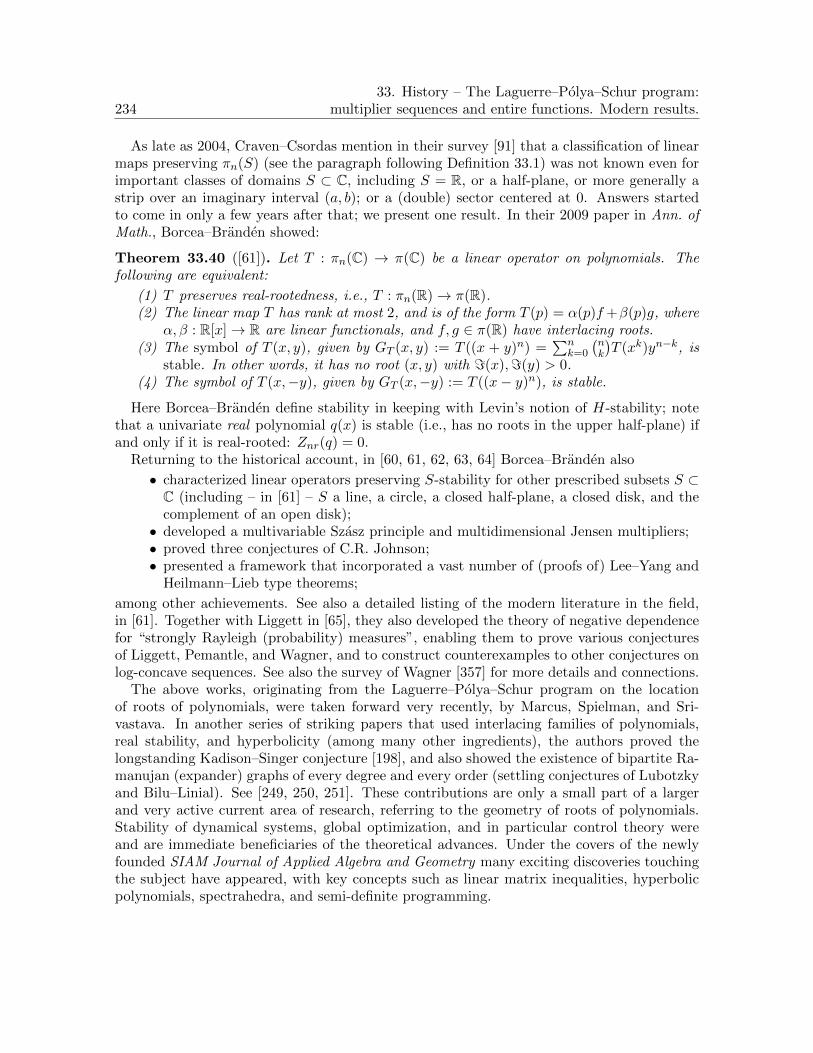
23433. History – The Laguerre–Polya–Schur program:

multiplier sequences and entire functions. Modern results.

As late as 2004, Craven–Csordas mention in their survey [91] that a classification of linearmaps preserving πn(S) (see the paragraph following Definition 33.1) was not known even forimportant classes of domains S ⊂ C, including S = R, or a half-plane, or more generally astrip over an imaginary interval (a, b); or a (double) sector centered at 0. Answers startedto come in only a few years after that; we present one result. In their 2009 paper in Ann. ofMath., Borcea–Branden showed:

Theorem 33.40 ([61]). Let T : πn(C) → π(C) be a linear operator on polynomials. Thefollowing are equivalent:

(1) T preserves real-rootedness, i.e., T : πn(R)→ π(R).(2) The linear map T has rank at most 2, and is of the form T (p) = α(p)f+β(p)g, where

α, β : R[x]→ R are linear functionals, and f, g ∈ π(R) have interlacing roots.(3) The symbol of T (x, y), given by GT (x, y) := T ((x + y)n) =

∑nk=0

(nk

)T (xk)yn−k, is

stable. In other words, it has no root (x, y) with =(x),=(y) > 0.(4) The symbol of T (x,−y), given by GT (x,−y) := T ((x− y)n), is stable.

Here Borcea–Branden define stability in keeping with Levin’s notion of H-stability; notethat a univariate real polynomial q(x) is stable (i.e., has no roots in the upper half-plane) ifand only if it is real-rooted: Znr(q) = 0.

Returning to the historical account, in [60, 61, 62, 63, 64] Borcea–Branden also

• characterized linear operators preserving S-stability for other prescribed subsets S ⊂C (including – in [61] – S a line, a circle, a closed half-plane, a closed disk, and thecomplement of an open disk);• developed a multivariable Szasz principle and multidimensional Jensen multipliers;• proved three conjectures of C.R. Johnson;• presented a framework that incorporated a vast number of (proofs of) Lee–Yang and

Heilmann–Lieb type theorems;

among other achievements. See also a detailed listing of the modern literature in the field,in [61]. Together with Liggett in [65], they also developed the theory of negative dependencefor “strongly Rayleigh (probability) measures”, enabling them to prove various conjecturesof Liggett, Pemantle, and Wagner, and to construct counterexamples to other conjectures onlog-concave sequences. See also the survey of Wagner [357] for more details and connections.

The above works, originating from the Laguerre–Polya–Schur program on the locationof roots of polynomials, were taken forward very recently, by Marcus, Spielman, and Sri-vastava. In another series of striking papers that used interlacing families of polynomials,real stability, and hyperbolicity (among many other ingredients), the authors proved thelongstanding Kadison–Singer conjecture [198], and also showed the existence of bipartite Ra-manujan (expander) graphs of every degree and every order (settling conjectures of Lubotzkyand Bilu–Linial). See [249, 250, 251]. These contributions are only a small part of a largerand very active current area of research, referring to the geometry of roots of polynomials.Stability of dynamical systems, global optimization, and in particular control theory wereand are immediate beneficiaries of the theoretical advances. Under the covers of the newlyfounded SIAM Journal of Applied Algebra and Geometry many exciting discoveries touchingthe subject have appeared, with key concepts such as linear matrix inequalities, hyperbolicpolynomials, spectrahedra, and semi-definite programming.

34. Schoenberg’s results on Polya frequency functions. 235

34. Schoenberg’s results on Polya frequency functions.

Having discussed the Laguerre–Polya entire functions and the Polya–Schur multiplier se-quences, we return to our primary objects of interest: Polya frequency functions. The goalin this section is to discuss some of the foundational results on these functions.

We first recall the definition of these functions and two closely related classes of functions:

Definition 34.1. Suppose Λ : R→ [0,∞) is Lebesgue measurable.

(1) Λ is said to be totally non-negative (TN) if given an integer p ≥ 1 and tuples x,y ∈Rp,↑, detTΛ[x; y] := det(Λ(xj − yk))pj,k=1 ≥ 0.

(2) We will say Λ is non-Dirac if Λ does not vanish at least at two points.(3) Λ is a Polya frequency (PF) function if Λ is non-monotone – equivalently, integrable

with mass a positive real number.

The equivalence in the third assertion was proved in Proposition 29.3(3).

Remark 34.2 (Non-Dirac TN functions). The functions in Definition 34.1(2) were termedtotally positive functions by Schoenberg – recall that in his papers and Karlin’s book, andeven later, TN and TP matrices/functions were termed TP and STP , i.e., (strictly) totallypositive. Finally, by Theorem 28.4, a non-Dirac TN function is strictly positive on an intervalof positive length, and continuous on its interior.

34.1. Precursors by Polya and Hamburger. We now discuss the origins of Polya fre-quency functions. Recall that in his 1951 paper [323], Schoenberg proved the variationdiminishing property for Polya frequency functions Λ, in terms of the values of functions aswell as for real zeros of polynomials. (See Propositions 29.15 and 29.17, respectively.) Tothe collection of prior results proved about the variation diminishing property – including forpower series by Fekete in 1912 [118] and for matrices by Schoenberg in 1930 [310], Motzkinin 1936 in his thesis [262], and others including prominently by Gantmacher–Krein – we nowadd a result shown in 1915 by Polya, in connection with the Laguerre–Polya class LP2.

Specifically, Polya studied the reciprocal of a function Ψk(s) ∈ LPk for k = 1, 2, whereΨk(0) > 0. He expanded the meromorphic function 1/Ψk as:

1

Ψk(s)=

∞∑j=0

(−1)j

j!µjs

j (34.3)

Polya then applied the differential operator 1/Ψ2(∂) to a real polynomial p(x), via

1

Ψ2(∂)p(x) = µ0p(x)− µ1p

′(x) + µ2p′′(x)

2!− · · · ± µn

p(n)(x)

n!, (34.4)

in the spirit of the preceding section, and where n = deg(p) ≥ 0. Notice that since ∂ islocally nilpotent on C[x], every formal power series in ∂ yields a well-defined operator onC[x], yielding an algebra homomorphism T from C[[s]] to linear operators on C[x].

With these preliminaries, as a first result Polya showed another condition equivalent tobeing in the second Laguerre–Polya class, i.e., a multiplier sequence of the second kind:

Theorem 34.5 ([284]). Given a formal power series ψ(s) :=∑

j≥0 µj(−s)j/j! with µ0 > 0,the following are equivalent:

(1) Given a polynomial p ∈ R[x], ψ(∂)(p(x)) has no more real roots than p(x):

Znr(ψ(∂)p(x)) ≥ Znr(p(x)).

(2) Ψ2(s) := 1/ψ(s) is in the Laguerre–Polya class LP2.

236 34. Schoenberg’s results on Polya frequency functions.

Proof-sketch. First, given the algebra homomorphism T sending a power series ψ(s) to ψ(∂),and since ψ(0) > 0, the assertion (1) can be rephrased as:

(1′) Let Ψ2(s) := 1/ψ(s). If p ∈ R[x], then Ψ2(∂)p has at least as many real roots as p.

We now show that (2) =⇒ (1′). If Ψ2 is constant then (1′) is immediate; else approximateΨ2(s) locally uniformly by a sequence of real-rooted polynomials ψn(s); since µ0 = Ψ2(0) > 0and Ψ2 is non-constant, the same holds for ψn for n 0. In particular, for large n, theHermite–Poulain theorem yields Znr(ψn(∂)p) ≤ Znr(p); and we also have deg(ψn(∂)p) =deg(p) = deg(Ψ2(∂)p). Hence Znr(Ψ2(∂)p) ≤ Znr(p) by the continuity of roots.

Conversely, we assume (1′) and show (2). Let g(x) := xn for some n ≥ 0. If Ψ2(s) =∑j≥0 νjs

j/j!, then by (1′), the polynomial

Ψ2(∂)(xn) =n∑j=0

(n

j

)νjx

n−j

has at least n roots, whence is real-rooted for n ≥ 0. Define the real sequence N :=(ν0, ν1, . . . ); thus Ψ2(∂)(xn) = N[(1 + x)n] is real-rooted for all n ≥ 0. It follows by thePolya–Schur characterizations of multiplier sequences of the second kind (see Theorem 33.30)that ΨN(x) = N[ex] = Ψ2(x) is in the class LP2, as desired.

Thus, Polya showed that Ψ2(∂) weakly increases (i.e., does not decrease) the number ofreal roots. We return to this result and proof presently; first we continue with the accountof Polya’s work [284]. Another result dealt with the reciprocal functions 1/Ψk(s), k = 1, 2:

Theorem 34.6 (Polya, [284]). Suppose Ψk(s) ∈ LPk for k ∈ 1, 2 is such that Ψk(0) > 0and Ψk(x) 6≡ Ceδx. Let 1/Ψk(s) =

∑j≥0 µj(−s)j/j!, and define the Hankel matrices

Hµ,j,n :=

µj µj+1 · · · µj+nµj+1 µj+2 · · · µj+n+1

......

. . ....

µj+n µj+n+1 · · · µj+2n

, j ≥ 0.

Then detHµ,0,n > 0 ∀n ≥ 0. If k = 1 then moreover detHµ,1,n > 0 ∀n ≥ 0.

Proof-sketch. Polya first showed in [284, Satz II and Satz III] the following claim:“Suppose k = 1 or 2, and a function Ψk is as in the assumptions. If a non-zero real

polynomial is non-negative on R and k = 2 (respectively, non-negative on [a,∞) and k = 1for some a ∈ R), then the polynomial 1

Ψk((−1)k∂)p is always positive on R (respectively, on

[a,∞)).”Now to prove detHµ,0,n > 0, choose a non-zero vector u = (u0, . . . , un)T ∈ Rn+1, and set

p(x) := (∑n

j=0 ujxj)2. By the previous paragraph and a straightforward computation,

0 <1

Ψ2(∂)p

∣∣∣∣x=0

= µ0u20−µ1(u0u1+u1u0)+µ2(u0u2+u2

1+u2u0)−· · · =n∑

j,k=0

(−1)j+kµj+kujuk.

Since this inequality holds for all non-zero vectors u, the matrix ((−1)j+kµj+k)nj,k=0 has

positive determinant by Sylvester’s criterion (Theorem 2.8). But Hµ,0,n is obtained from thismatrix by pre- and post-multiplication by the matrix diag(1,−1, 1, . . . , (−1)n−1).

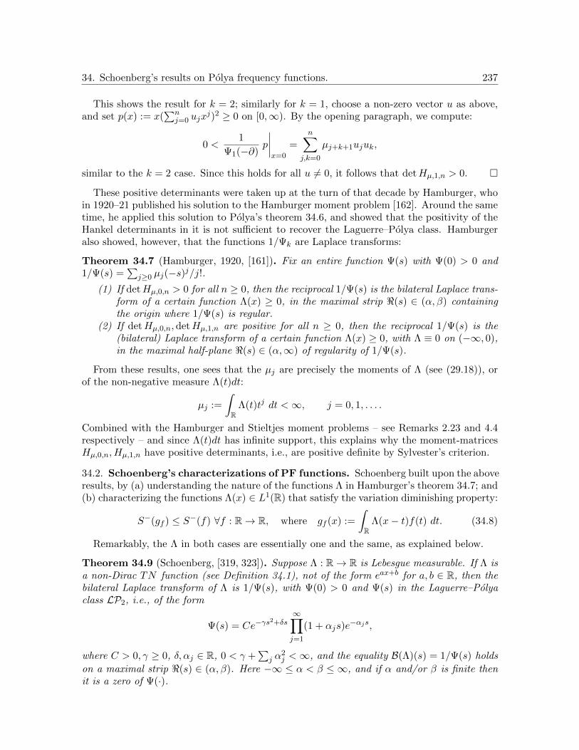
34. Schoenberg’s results on Polya frequency functions. 237

This shows the result for k = 2; similarly for k = 1, choose a non-zero vector u as above,and set p(x) := x(

∑nj=0 ujx

j)2 ≥ 0 on [0,∞). By the opening paragraph, we compute:

0 <1

Ψ1(−∂)p

∣∣∣∣x=0

=n∑

j,k=0

µj+k+1ujuk,

similar to the k = 2 case. Since this holds for all u 6= 0, it follows that detHµ,1,n > 0.

These positive determinants were taken up at the turn of that decade by Hamburger, whoin 1920–21 published his solution to the Hamburger moment problem [162]. Around the sametime, he applied this solution to Polya’s theorem 34.6, and showed that the positivity of theHankel determinants in it is not sufficient to recover the Laguerre–Polya class. Hamburgeralso showed, however, that the functions 1/Ψk are Laplace transforms:

Theorem 34.7 (Hamburger, 1920, [161]). Fix an entire function Ψ(s) with Ψ(0) > 0 and1/Ψ(s) =

∑j≥0 µj(−s)j/j!.

(1) If detHµ,0,n > 0 for all n ≥ 0, then the reciprocal 1/Ψ(s) is the bilateral Laplace trans-form of a certain function Λ(x) ≥ 0, in the maximal strip <(s) ∈ (α, β) containingthe origin where 1/Ψ(s) is regular.

(2) If detHµ,0,n,detHµ,1,n are positive for all n ≥ 0, then the reciprocal 1/Ψ(s) is the(bilateral) Laplace transform of a certain function Λ(x) ≥ 0, with Λ ≡ 0 on (−∞, 0),in the maximal half-plane <(s) ∈ (α,∞) of regularity of 1/Ψ(s).

From these results, one sees that the µj are precisely the moments of Λ (see (29.18)), orof the non-negative measure Λ(t)dt:

µj :=

∫R

Λ(t)tj dt <∞, j = 0, 1, . . . .

Combined with the Hamburger and Stieltjes moment problems – see Remarks 2.23 and 4.4respectively – and since Λ(t)dt has infinite support, this explains why the moment-matricesHµ,0,n, Hµ,1,n have positive determinants, i.e., are positive definite by Sylvester’s criterion.

34.2. Schoenberg’s characterizations of PF functions. Schoenberg built upon the aboveresults, by (a) understanding the nature of the functions Λ in Hamburger’s theorem 34.7; and(b) characterizing the functions Λ(x) ∈ L1(R) that satisfy the variation diminishing property:

S−(gf ) ≤ S−(f) ∀f : R→ R, where gf (x) :=

∫R

Λ(x− t)f(t) dt. (34.8)

Remarkably, the Λ in both cases are essentially one and the same, as explained below.

Theorem 34.9 (Schoenberg, [319, 323]). Suppose Λ : R→ R is Lebesgue measurable. If Λ isa non-Dirac TN function (see Definition 34.1), not of the form eax+b for a, b ∈ R, then thebilateral Laplace transform of Λ is 1/Ψ(s), with Ψ(0) > 0 and Ψ(s) in the Laguerre–Polyaclass LP2, i.e., of the form

Ψ(s) = Ce−γs2+δs

∞∏j=1

(1 + αjs)e−αjs,

where C > 0, γ ≥ 0, δ, αj ∈ R, 0 < γ +∑

j α2j <∞, and the equality B(Λ)(s) = 1/Ψ(s) holds

on a maximal strip <(s) ∈ (α, β). Here −∞ ≤ α < β ≤ ∞, and if α and/or β is finite thenit is a zero of Ψ(·).

238 34. Schoenberg’s results on Polya frequency functions.

Conversely, if Ψ ∈ LP2 is as above, then 1/Ψ(s) is the (bilateral) Laplace transform of anon-Dirac TN function Λ, not of the form eax+b for a, b ∈ R.

In particular, the condition 0 < γ +∑

j α2j <∞ implies that Ψ(s) is not of the form Ceδs.

Moreover, in light of Proposition 29.3, one can translate the maximal strip by multiplying byan exponential factor:

Corollary 34.10. Given a non-Dirac TN function Λ : R→ R, the following are equivalent:

(1) Λ is a Polya frequency function.(2) The maximal strip in the preceding theorem contains the imaginary axis.(3) Λ is non-monotone.(4) Λ is integrable.

The above results were for general Polya frequency functions (or non-Dirac TN functions)vis-a-vis the Laguerre–Polya class LP2. The corresponding equivalence for one-sided TN/PFfunctions was also shown by Schoenberg, in the same works [319, 323]:

Theorem 34.11. Suppose Λ : R → R is Lebesgue measurable. If Λ is a non-Dirac TNfunction, vanishing on (−∞, 0), and such that B(Λ)(s) converges for <(s) > 0 (in particularnot an exponential eax+b for a > 0), then the bilateral Laplace transform of Λ is 1/Ψ(s), withΨ(s) > 0 for s > 0 and Ψ(s) in the Laguerre–Polya class LP1, i.e., of the form

Ψ(s) = Ceδs∞∏j=1

(1 + αjs),

where C > 0, δ, αj ≥ 0, 0 <∑

j αj < ∞, and the equality B(Λ)(s) = 1/Ψ(s) holds on a

maximal strip <(s) ∈ (α,∞). Here α denotes the first zero of Ψ(·).Conversely, if Ψ ∈ LP2 is as above, then 1/Ψ(s) is the (bilateral) Laplace transform of a

non-Dirac TN function Λ with the aforementioned properties.Moreover, such a function Λ is a Polya frequency function if and only if Ψ(0) > 0.

Note that Ψ(0) > 0 if and only if Λ is integrable; thus it cannot be constant on (0,∞).Schoenberg’s theorems 34.9 and 34.11 characterize non-Dirac TN functions and Polya

frequency functions, both one- and two-sided, in terms of the Laguerre–Polya class.

Proof-sketch of Theorem 34.9. In the concluding portion of Section 32 (see the discussionaround (32.16) and (32.17)) we saw an outline of why for k = 1, 2, the function 1/Ψk(s) forany Ψk ∈ LPk is the Laplace transform of a Polya frequency function (one-sided or general,for k = 1, 2 respectively). We outline here a proof of why the reverse implication holds fork = 2. The outline opens with Schoenberg’s words [319]:

“A proof of Theorem 34.9 is essentially based on the results and methods developed by Polyaand Schur. The only additional element required is a set of sufficient conditions insuring thata linear transformation be variation diminishing.”

This last sentence of Schoenberg refers to his 1930 paper, in which he showed that TN ma-trices are variation diminishing. Using this property, he showed the same for Polya frequencyfunctions, whence for polynomials (and then did the same for one-sided PF functions); seeSection 29.2. Now suppose Λ is a PF function; we proceed to outline the proof of why B(Λ),which converges on a maximal strip <(s) ∈ (α, β) with α < 0 < β, is of the form 1/Ψ2(s) forΨ2(s) in the Laguerre–Polya class LP2. Following Polya, write

B(Λ)(s) =∞∑j=0

(−1)j

j!µjs

j , <(s) ∈ (α, β),

34. Schoenberg’s results on Polya frequency functions. 239

where µj =∫R Λ(t)tj dt are the moments, as discussed after Theorem 34.7. Also note that

B(Λ)(0) = µ0 > 0, so we write the reciprocal power series:

Ψ2(s) :=1

B(Λ)(s)=∞∑j=0

νjj!sj .

Now return to the integral transformation f 7→ gf as in (34.8). By Proposition 29.17,Z(gf ) ≤ Z(f), where Z(·) denotes the number of real roots. Next, recall Schoenberg’scomputation (29.19), perhaps inspired by Polya’s trick (34.4):

gf (x) =

∫R

Λ(t)f(x− t) dt =∞∑j=0

(−1)j

j!µj(∂

jf)(x) = (B(Λ)(∂)f)(x).

We use here that both sides are polynomials, so that only finitely many terms µj∂j act

nontrivially. Now take the reciprocal power series, e.g. via the map T following (34.4), toobtain: f(x) = Ψ2(∂)(gf )(x). In fact since f 7→ gf is invertible (see the proof of Proposi-tion 29.17), the linear operator g 7→ fg := Ψ2(∂)g is also invertible, and it weakly increasesthe number of real roots. Finally, use (1′) =⇒ (2) in the proof of Polya’s theorem 34.5.

Remark 34.12. Thus, Schoenberg showed in [320, 323] the connection between his charac-terization of PF functions via the Laguerre–Polya class, Polya–Schur multipliers, and Polya’stheorem 34.5 proving the variation diminishing property over polynomials. This explains whySchoenberg proposed in [320] the name Polya frequency functions for this family of functions.

We conclude with another characterization of Polya frequency functions, which Schoenbergannounced in [320] and showed in [322]. This occurs via the variation diminishing property:

Theorem 34.13 (Schoenberg, [320, 322]). Given Λ : R → R Lebesgue integrable, let thekernel f 7→ gf as in (34.8), for continuous, bounded f : R→ R. The following are equivalent:

(1) Λ is variation diminishing: S−R (gf ) ≤ S−R (f) for all continuous, bounded f : R→ R.(2) One of ±Λ is a PF function, or Λ is a Dirac function C1x=a for some C, a ∈ R.

Thus, the converse to Proposition 29.15 holds as well. For yet another characterization ofPolya frequency functions – in terms of splines – see [95, 96] by Curry and Schoenberg.

34.3. Support of PF functions; (strict) total positivity. We now discuss two conse-quences of the above results, which were also proved by Schoenberg. The first is that a Polyafrequency function necessarily cannot be compactly supported:

Proposition 34.14. The support of a Polya frequency function Λ : R→ R is unbounded.

Recall by Theorem 28.4 that the support of a TN2 function is an interval, so in fact thesupport of a PF function now must be of the form (a, b) where at least one of |a|, |b| is infinite.

Proof. We already know the support of a Polya frequency function is not a singleton. Let Ibe a bounded interval with endpoints −∞ < a < b <∞. The claim is that for any functionΛ : R→ R supported on I and continuous in its interior, the Laplace transform

B(Λ)(s) :=

∫ b

ae−sxΛ(x) dx, s ∈ C

is entire, with kth derivative (−1)k∫ ba e−sxxkΛ(x) dx. Indeed, one shows that the series

∞∑n=0

(−s)n

n!

∫ b

axnΛ(x) dx

240 34. Schoenberg’s results on Polya frequency functions.

is uniformly convergent for s in any bounded domain in C. Hence its sum is entire, andequals B(Λ)(s); moreover, one can differentiate term by term to compute its kth derivative:

∞∑n=k

sn−k

(n− k)!

∫ b

a(−x)nΛ(x) dx =

∫ b

ae−sx(−x)kΛ(x) dx.

Having shown the claim, we proceed to the proof. By Theorem 34.9,

B(Λ)(s) = C−1eγs2−δs

∞∏j=1

eαjs

1 + αjs, (34.15)

for appropriate values of the parameters. Now if Λ has bounded support, then from above

the right-hand side is entire. It follows that αj = 0 ∀j. But then B(Λ)(s) = C−1eγs2−δs.

Now by Laplace inversion and Example 29.4, Λ itself is a (shifted) Gaussian density, hencehas unbounded support. This provides the necessary contradiction.

The final result here, due to Schoenberg and Whitney in Trans. Amer. Math. Soc. (1953),provides a sufficient condition when a Polya frequency function is (strictly) totally positive.We mention only a part of their results, and show only the sub-part relevant for our purposes.

Theorem 34.16 (Schoenberg–Whitney).

(1) If Λ+,Λ0 : R→ R are PF functions, and Λ+ yields a TP kernel, then so does Λ+∗Λ0.(2) Suppose Λ(x) has bilateral Laplace transform (34.15). If γ > 0, or γ = 0 and

∑j |aj |

diverges, then the kernel TΛ is TP (of all orders).

Proof. For the first part: that Λ+ ∗Λ0 is a PF function follows from Corollary 32.9. We nowclaim that given p ≥ 1 and y ∈ Rp,↑, there exists t = (t1, . . . , tp) ∈ Rp,↑ such that TΛ0 [t; y] isnon-singular. The proof is by induction on p ≥ 1; for the base case, since

∫R Λ0(x) dx ∈ (0,∞),

it is positive on an interval, so we can choose t1 as desired.For the induction step, let p ≥ 2 and y ∈ Rp,↑. Choose t := (t1, . . . , tp−1) ∈ Rp−1,↑ such

that the matrix (Λ0(tj − yk))p−1j,k=1 is non-singular, whence has positive determinant since Λ0

is TN . Now expand the determinant of TΛ0 [(t; t); y] along the last row; if this vanishes forall t ∈ R, we obtain an equation

∑pk=1 akΛ0(t−yk) ≡ 0, where all ak ∈ R and ap > 0. Taking

the bilateral Laplace transform of both sides,

ψ(s)

p∑k=1

ake−syk

must vanish for s in some interval, where ψ 6≡ 0 by the Schoenberg representation theorems.Hence the sum vanishes identically on an interval – which is false by Descartes’ rule of signs(Theorem 10.3). Thus, TΛ0 [(t; t); y] is non-singular for some t ∈ R. Clearly t 6= tj ∀j, so bysuitably permuting the rows (and relabeling the t, tj if needed), the induction step is proved.

Having shown the claim, and using the continuity on an interval of both Λ+,Λ0, one checksusing the Basic Composition Formula (5.14) that Λ+ ∗ Λ0 is TPp for each p ≥ 1:

det((Λ+∗Λ0)(xi−yk))pi,k=1 =

∫· · ·∫

t1<t2<···<tm in R

det(Λ+(xi−tj))pi,j=1 det(Λ0(tj−yk))pj,k=1

p∏j=1

dµ(yk).

We only (require, hence) show the second part for γ > 0. By Theorem 34.9, e−γs2/2B(Λ)(s)

is the bilateral Laplace transform of a PF function, say Λ0; and eγs2/2 of a TP (Gaussian)

PF function Λ+, say by Example 29.4. By the preceding part, Λ = Λ+ ∗ Λ0 is TP .

35. Further one-sided examples: The Hirschman–Widder densities.Discontinuous PF functions. 241

35. Further one-sided examples: The Hirschman–Widder densities.Discontinuous PF functions.

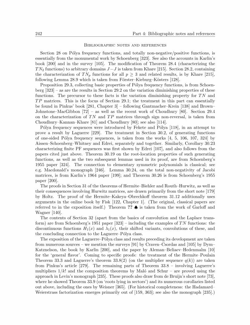
242 Part 4: Bibliographic notes and references

Bibliographic notes and references

Section 28 on Polya frequency functions, and totally non-negative/positive functions, isessentially from the monumental work by Schoenberg [323]. See also the accounts in Karlin’sbook [200] and in the survey [105]. The modification of Theorem 28.4 (characterizing theTN2 functions) to arbitrary domains J−J is taken from Khare [215]. Section 28.2, containingthe characterization of TNp functions for all p ≥ 3 and related results, is by Khare [215],following Lemma 28.9 which is taken from Forster–Kieburg–Kosters [128].

Proposition 29.3, collecting basic properties of Polya frequency functions, is from Schoen-berg [323] – as are the results in Section 29.2 on the variation diminishing properties of thesefunctions. The precursor to these facts is the variation diminishing property for TN andTP matrices. This is the focus of Section 29.1; the treatment in this part can essentiallybe found in Pinkus’ book [281, Chapter 3] – following Gantmacher–Krein [138] and Brown–Johnstone–MacGibbon [72] – as well as the recent work of Choudhury [80]. Section 29.4on the characterization of TN and TP matrices through sign non-reversal, is taken fromChoudhury–Kannan–Khare [81] and Choudhury [80]; see also [114].

Polya frequency sequences were introduced by Fekete and Polya [118], in an attempt toprove a result by Laguerre [229]. The treatment in Section 30.2, of generating functionsof one-sided Polya frequency sequences, is taken from the works [4, 5, 106, 107, 324] byAissen–Schoenberg–Whitney and Edrei, separately and together. Similarly, Corollary 30.23characterizing finite PF sequences was first shown by Edrei [107], and also follows from thepapers cited just above. Theorem 30.19 on the root-location properties of such generatingfunctions, as well as the two subsequent lemmas used in its proof, are from Schoenberg’s1955 paper [324]. The connection to elementary symmetric polynomials is classical; seee.g. Macdonald’s monograph [246]. Lemma 30.24, on the total non-negativity of Jacobimatrices, is from Karlin’s 1964 paper [199]; and Theorem 30.26 is from Schoenberg’s 1955paper [200].

The proofs in Section 31 of the theorems of Hermite–Biehler and Routh–Hurwitz, as well astheir consequences involving Hurwitz matrices, are drawn primarily from the short note [179]by Holtz. The proof of the Hermite–Kakeya–Obrechkoff theorem 31.12 additionally usesarguments in the online book by Fisk [122, Chapter 1]. (The original, classical papers arereferred to in the exposition itself.) Theorem ?? ♠ is taken from the work of Garloff andWagner [140].

The contents of Section 32 (apart from the basics of convolution and the Laplace trans-form) are from Schoenberg’s 1951 paper [323] – including the examples of TN functions: thediscontinuous functions H1(x) and λ1(x), their shifted variants, convolutions of these, andthe concluding connection to the Laguerre–Polya class.

The exposition of the Laguerre–Polya class and results preceding its development are takenfrom numerous sources – we mention the surveys [91] by Craven–Csordas and [105] by Dym–Katznelson, the book by Karlin [200], and the paper by Aleman–Beliaev–Hedenmalm [10]for the ‘general flavor’. Coming to specific proofs: the treatment of the Hermite–PoulainTheorem 33.3 and Laguerre’s theorem 33.8(2) (on the multiplier sequence q(k)) are takenfrom Pinkus’s article [279]. The remaining parts of Theorem 33.8 – involving Laguerre’smultipliers 1/k! and the composition theorems by Malo and Schur – are proved using theapproach in Levin’s monograph [235]. These proofs also draw from de Bruijn’s short note [73],where he showed Theorem 33.9 (on ‘roots lying in sectors’) and its numerous corollaries listedout above, including the ones by Weisner [365]. (For historical completeness: the Hadamard–Weierstrass factorization emerges primarily out of [159, 363]; see also the monograph [235].)

Part 4: Bibliographic notes and references 243

Theorems 34.5 and 34.6, involving early findings of Polya about functions 1/Ψ(s) for Ψin the Laguerre–Polya class, are taken from [284]. Theorem 34.7, showing that 1/Ψ(s) hasa Laplace transform representation, is taken from Hamburger’s paper [161]. Section 34.2,containing characterizations of Polya frequency functions (both general or one-sided) interms of the Laguerre–Polya class or variation diminution, is taken from the two announce-ments [319, 320] and the subsequent ‘full papers’ [322, 323] by Schoenberg. Proposition 34.14on the unbounded support of a Polya frequency function is from [323], and Theorem 34.16on the total positivity of certain PF functions is from Schoenberg and Whitney’s paper [326].

Part 5:

Composition operators preservingtotally positive kernels

36. Critical exponent for powers preserving TNp. The Jain–Karlin–Schoenberg kernel. 247

Part 5: Composition operators preserving totally positive kernels

36. Critical exponent for powers preserving TNp. TheJain–Karlin–Schoenberg kernel.

Having classified – in a previous part of this text – the preservers of Loewner positivity,monotonicity, and convexity on infinite domains, we now turn to preservers of total non-negativity and total positivity. This section is concerned with preservers of TNp for p finite,with emphasis on power functions. In particular, we will see the occurrence of a criticalexponent phenomenon in total positivity – this time for powers of one-sided TNp functions.

36.1. Connections to representation theory and probability. We end this second lookat critical exponents (the first was in Part 2 of this text) by providing connections to otherareas of mathematics – specifically, via the Wallach set (or Gindikin ensemble, or Berezin–Wallach set). The following is a very brief account of these topics, and the references hereshould provide the reader with starting points for further exploration into this rich area, atthe intersection of representation theory, complex analysis, and probability.

Suppose n ≥ 1 and D ⊂ Cn is a tube domain, i.e., of the form D = Rn + iΩ, where Ω is ahomogeneous irreducible self-dual convex cone in Rn. Denote by H1 the associated Bergmanspace, consisting of holomorphic functions F on D satisfying:∫

D|F (x+ iy)|2 dxdy <∞,

and let H2 denote the Hardy space, consisting of holomorphic functions F on D satisfying:

supy∈Ω

∫Rn|F (x+ iy)|2 dx <∞.

Let P (z − w) denote the Bergman kernel on D; thus F (w) = 〈F, Pw〉H1 for all F ∈ H1,where Pw(z) := P (z − w). Then the Hardy space H2 has a reproducing kernel of the formP p, for some power p < 1 of the Bergman kernel. In Acta Math. (1976), Rossi and Vergneclassified the powers of P which are reproducing kernels for some Hilbert space of holomorphicfunctions on D. They called the set of such powers p the Wallach set, and showed in [302]that it consists of an arithmetic progression and a half-line: 0, c/r, 2c/r, . . . , c t (c,∞) forsome c > 0 and r ≥ 0. The exact meaning of p, c, r can be found in [302].

Rossi–Vergne named the aforementioned set after Wallach, who was studying it at the time(note, Wallach’s papers [358] appeared in print later, in 1979 in Trans. Amer. Math. Soc.).Wallach, following up on work of Harish-Chandra, was studying the holomorphic discreteseries of connected, simply connected Lie groups G. Specifically, he classified the set of twist-parameters p of the center of K (a maximal compact reductive subgroup of G) for which thecorresponding K-finite highest weight module over g = Lie(G) (complexified) is irreducibleand unitarizable, or it is reducible and its radical is unitarizable. In [302], Rossi and Vergneobtained the same (Wallach) set of parameters p, with the sufficiently large p leading tothe holomorphic discrete series of weighted Bergman spaces. See also [116], where Farautand Koranyi worked over symmetric domains D, and studied Hilbert spaces of holomorphicfunctions on D.

The Wallach set also appears in at least two other settings, both again in the 1970s:

• Berezin [38] had encountered such a set while studying Kahler potentials of Siegeldomains, in the context of quantization. (See also [268] for a recent avatar of thisset of exponents, defined in the context of positive semidefinite kernels and recallingvarious results discussed above).

248 36. Critical exponent for powers preserving TNp. The Jain–Karlin–Schoenberg kernel.

• Gindikin [143] had shown that given a symmetric cone, and a Riesz distribution Rµassociated to it, Rµ is a positive measure if and only if µ ∈ C lies in an associatedWallach set. A simple proof of this result (and more) was given in 2011 by Sokal [343].

On a conceptual note: the work of Gindikin on the Wallach set arises throughratios of gamma functions on symmetric cones, which are of the form G/K for agroup G and a maximal compact subgroup K. Now, the ‘usual’ gamma function canbe defined via the Laplace transform on the cone R+. In fact, this can be done overarbitrary symmetric cones in Euclidean Jordan algebras – for instance, in the conePn(R) ∼= GLn(R)/On(R), where G = GLn,K = On stand for the general linear andorthogonal groups of n× n real matrices, respectively.

Via the Iwasawa decomposition G = K ·A ·N , carrying out the Laplace transformon such a cone G/K is the same as doing so on A ·N . This turns out to be a solvablegroup, and the associated Haar measure is closely related to Lebesgue measure. Thisprovides a ‘natural’ setting for Gindikin’s work and for proving his results – see the1991 paper of Kostant–Sahi [226] in Adv. Math. for details. As the authors remark,the main ingredient in the above working is the Laplace transform on a self-dual cone;the origins of this can be found in the 1935 paper [335] of Siegel in Ann. of Math.(see also the book of Hua [185]).

Gindikin’s work leads us to another recent manifestation of the critical exponent in matrixanalysis – specifically, in random matrix theory. We first mention the 1987 paper [232] ofLassalle in Invent. Math., which approached the same problem through the formalism ofpositive cones in formally real Jordan algebras. Lassalle recovered the results of Wallach andRossi–Vergne concerning the Wallach set.

The results of Gindikin, Berezin, Rossi–Vergne, Wallach, and Lassalle can all be interpretedin the language of shape parameters of (non-central) Wishart distributions. We begin withthe more standard ‘central’ Wishart distribution, defined by Wishart in 1920 [370]. One wayto define this is through the Laplace transform of its density function. More precisely, fix aninteger n ≥ 1; now given the shape parameter p ∈ [0,∞) and the scale parameter Σ, whichis a positive definite n × n real matrix, Γ(p,Σ) denotes the Wishart distribution, say withdensity f , satisfying:

LΓ(p,Σ)(s) :=

∫Pn(R)

e−tr(sA) f(dA) equals det(Idn×n +2sΣ)−p, s ∈ Pn(R).

It is a well-known fact (see e.g. [117]) that such a distribution exists if and only if p is inthe Wallach set 0, 1/2, . . . , (n− 2)/2 t (((n− 1)/2),∞).

We now come to recent work along these lines. The non-central Wishart distribution issimilarly defined – now also using a non-centrality parameter Ω ∈ Pn(R) – via its Laplacetransform

LΓ(p,Σ,Ω)(s) = det(Idn×n +2sΣ)−pe−2tr(ΩsΣ(Idn×n +2sΣ)−1), s ∈ Pn(R).

In 2018, Graczyk–Malecki–Mayerhofer [145] and Letac–Massam [234] showed (akin toabove) that such a distribution exists if and only if (a) p belongs to the same Wallach set asabove:

p ∈ 0, 1/2, . . . , (n− 2)/2 t (((n− 1)/2),∞),

and (b) if p < (n − 1)/2 then rk Ω ≤ 2p. The same result was shown by Mayerhoferin Trans. Amer. Math. Soc. in 2019, building on ideas of Faraut [115] (1988) and Peddada–St. Richards [276] (1991). To do so, Mayerhofer [254] extended prior analysis by the aforemen-tioned authors, on the positivity of generalized binomial coefficients that occur in Euclidean

36. Critical exponent for powers preserving TNp. The Jain–Karlin–Schoenberg kernel. 249

Jordan algebras. See e.g. [117] for an introduction to this; also see the 2011 work [307,Theorems 1 and 5] by Sahi, for stronger positivity results.

We end with a (superficial) relation between the Wallach set here and the set of powerspreserving positivity on Pn((0,∞)) (and total non-negativity of order n for the powers ofthe kernel TΩ) studied by FitzGerald–Horn, Karlin, and Jain. These powers were studied inSections 9 and 15 above, as well as in the present section. It would be interesting to find adeeper, conceptual connection between the two problems.

We begin with the positivity preservers side. Recall from the proof of Theorem 9.3 that ifα ∈ (0, n− 2) \Z, and x1, . . . , xn ∈ (0,∞) are pairwise distinct, then the Taylor expansion ofthe entrywise power ((1 + xjxk)

α)nj,k=1 yields

((1 + xjxk)α)nj,k=1 =

∑m≥0

(α

m

)xm(xm)T ,

where(αm

)= α(α − 1) · · · (α −m + 1)/m! and xm := (xm1 , . . . , x

mn )T . Now the key is that

for m = bαc + 2, the binomial coefficient is negative. Thus one can pre- and post-multiplythe above matrix by uT , u respectively, for some u ∈ Rn orthogonal to the smaller entrywisepowers of x. Using this, one can deduce that ((1 + xjxk)

α)nj,k=1 is not positive semidefinite.The connection to the Wallach set W is via the fact that the analysis for powers that

do not lie in W (to show that a (non)central Wishart distribution does not exist) also goesthrough the negativity of certain generalized binomial coefficients. As a simple example, welook into the argument in the aforementioned work of Peddada–Richards in Ann. Probab.1991. (A similar computation concludes the proof of [254, Theorem 4.10].) Given integersk1 ≥ · · · ≥ kn ≥ 0, define the shifted factorial by:

(p)k :=

n∏j=1

(p− 12(j − 1))kj , where (p)k := p(p+ 1) · · · (p+ k − 1)

if k > 0, and (p)0 := 1. Now it is shown in [276] – via the use of zonal polyomials – that if the(non)central Wishart density with shape parameter p exists, then (p)k ≥ 0 for all n-tuples kas above. But if q = 2p ∈ (0, n− 1) \ Z, then set

m := bqc+ 2, k1 = · · · = km = 1, km+1 = · · · = kn = 0.

Then the associated generalized binomial coefficient is

q

2

q − 1

2· · · q − bqc − 1

2· (1 · 1 · · · 1),

and this is negative by choice of q.

37. Preservers of Polya frequency functions. 251

37. Preservers of Polya frequency functions.

37.1. Preservers of TN functions.

37.2. Preservers of Polya frequency functions.

37.3. Preservers of TP Polya frequency functions.

38. Preservers of Polya frequency sequences. 253

38. Preservers of Polya frequency sequences.

Having classified the preservers of TN functions and their subclass of (TP ) Polya frequencyfunctions, we turn to such Toeplitz kernels on distinguished subsets. This section deals withPolya frequency sequence, i.e., Toeplitz TN kernels on Z×Z. However, several of the resultswill be shown to hold over more general domains X,Y ⊂ R with arbitrarily long arithmeticprogressions. The full power of these more general domains SX, Y will be revealed in thenext section, which concludes this part of the text.

As we saw in the previous three sections, working with kernels on intervals allows one touse powerful tools and results from analysis. These tools are also used in the present section,where we will use PF functions (on R × R) to classify the preservers of (TP ) PF sequences(on Z× Z).

38.1. Preservers of PF sequences.

38.2. Preservers of TP PF sequences. Discretization: if F is continuous and preservesPF sequences, then F preserves measurable TN Toeplitz kernels.

38.3. Preservers of one-sided PF sequences.

38.4. Further questions. To conclude this section, here are a few open questions involvingPolya frequency functions and sequences, and their preservers.

Question 38.1. In light of Schoenberg’s theorem 28.4 characterizing the TN2 functions,classify the preservers of these functions.

For example, the aforementioned theorems imply that all powers xα preserve the TNp

functions for p = 2, 3, if α ∈ Z≥0 ∪ [p − 2,∞). We also saw in ♣ that xα1x≥0 is a TNp

function if and only if α ∈ Z≥0 ∪ [p − 2,∞). In light of this, a natural question involvesstudying the powers preserving total non-negativity of each degree:

Question 38.2. Given an integer p ≥ 2, classify the powers xα which preserve the class ofTNp functions. Note by ♣ that every such power is in Z≥0 ∪ [p− 2,∞).

Coming to Polya frequency sequences, the above classification results lead to additional,theoretical questions about related sequences, which are mentioned for the interested reader.

Question 38.3. Classify the preservers of one-sided Polya frequency sequences: (i) thathave finitely many diagonals, or (ii) generated by evaluating a polynomial at non-negativeintegers.

Like a question above, both of these classes of functions have nontrivial power-preservers.Indeed, xn preserves both of these classes for all integers n ≥ 1, by Malo’s theorem 33.8 anda result of Wagner [356], respectively. Akin to the above discussion involving non-integer‘one-sided powers’ which are TNp, a related question is:

Question 38.4. Classify the power functions x 7→ xα, such that if∑

j ajxj is a polynomial

with positive coefficients and real roots, then so is∑

j aαj x

j . In particular, find the ‘criticalexponent’ αp for polynomials of a fixed degree p, such that every α ≥ αp satisfies this propertyon polynomials of degree at most p.

Note again by Malo’s theorem 33.8 that every integer α ≥ 1 satisfies this property. Re-cently, Wang and Zhang showed in [362] the existence of the threshold αp. Notice by ♣ that

254 38. Preservers of Polya frequency sequences.

this question is connected to entrywise powers preserving PF sequences with up to p non-zerodiagonals, and hence refines the preceding question.

A final, Whitney-type density question is:

Question 38.5. Are the totally positive Polya frequency sequences dense in the set of allPolya frequency sequences?

Such a result could help obtain the preservers of the TP PF sequences from the preserversof all PF sequences. (Note that this goal is achieved above via alternate means.)

39. Preservers of TP Hankel kernels. 255

39. Preservers of TP Hankel kernels.

In this section, we change gears, and work with a setting studied above for matrices: Hankelkernels, now defined on a sub-interval of R instead of on the integers 0, 1, . . . . As shouldbe clear from the previous sections, working with kernels on intervals (e.g. R×R) allows oneto use a host of powerful, classical techniques and results from analysis, which help proveresults even on discrete domains (e.g. Z× Z).

We begin with terminology. Given subsets X,Y ⊂ R, define their Minkowski sum X+Y :=x + y : x ∈ X, y ∈ Y . Now a kernel K : X × Y → R is said to be Hankel if there is afunction f : X + Y → R such that K(x, y) = f(x + y) for all x ∈ X, y ∈ Y . Note that ifX = Y then any such ‘square’ kernel is symmetric.

A natural class of such kernels in analysis is when X is an interval, and in this section wefocus on this case. In keeping with the above sections, here is a typical example of a HankelTN kernel: given finitely many positive scalars c1, . . . , cn, u1, . . . , un, define

Kc,u : R× R→ R, Kc,u(x, y) :=n∑j=1

cjux+yj .

We show in Theorem 39.6 that this kernel is TN on R × R (whence on X × X for anysub-interval X ⊂ R).

39.1. Preservers of Hankel TN kernels on intervals. In this section, we classify thepreservers of Hankel TN and TP kernels, on X×X for X an interval that is always assumedto have positive measure. The first main result addresses Hankel TN kernels:

Theorem 39.1. Let X ⊂ R be an interval with positive measure, and F a function : [0,∞)→R. The following are equivalent:

(1) The composition map F − preserves total non-negativity on the continuous HankelTN kernels on X ×X.

(2) The composition map F − preserves positive semidefiniteness on the continuousHankel TN kernels on X ×X.

(3) The function F is a power series with non-negative coefficients: F (x) =∑∞

k=0 ckxk

for x > 0, with all ck ≥ 0; and F (0) ≥ 0.

The proof of this result uses a discretization technique that will also be useful later:

Lemma 39.2 (Discretization of Hankel kernels). Suppose X ⊂ R is an interval with positivemeasure, and K : X ×X → R. Then each of the following statements implies the next.

(1) K is TN .(2) All principal submatrices drawn from K are TN .(3) All principal submatrices drawn from K, with arguments lying in an arithmetic pro-

gression, are TN .(4) All principal submatrices drawn from K, with arguments lying in an arithmetic pro-

gression, are positive semidefinite.

Conversely, (2) =⇒ (1) for all kernels, (3) =⇒ (2) for continuous kernels, and (4) =⇒ (3)for continuous Hankel kernels.

Proof. The forward implications are immediate from the definitions. Conversely, using thenotation in Definition 25.1, if x, z ∈ Xn,↑ for some n ≥ 1, then the matrix K[x; z] is asubmatrix of K[x ∪ z; x ∪ z], where x ∪ z denotes the union of the coordinates of x and z,together arranged in increasing order. Thus (2) =⇒ (1).

256 39. Preservers of TP Hankel kernels.

Now suppose K is continuous and (3) holds. We will show (2): given x1 < · · · < xn in X,

let ε := minj(xj+1 − xj)/2, and approximate each xj by a rational sequence z(k)j with:

z(k)1 ∈ [x1, x1 + ε), z(k)

n ∈ (xn − ε, xn], z(k)j ∈ (xj − ε, xj + ε), j ∈ (1, n).

Choose an integer Nk ≥ 1 such that z(k)j ∈ 1

NkZ for all k, and define:

z(k) := (z(k)1 , z

(k)1 +

1

Nk, z

(k)1 +

2

Nk, . . . , z(k)

n ), z(k)1 := (z

(k)1 , z

(k)2 , . . . , z(k)

n ).

By assumption, the matrix K[z(k); z(k)] is TN , whence so is the submatrix K[z(k)1 ; z

(k)1 ] for all

k. Let k →∞; since K is continuous, it follows that K[x; x] is TN , where x = (x1, . . . , xn).This shows (2).

Finally, suppose K is continuous and Hankel, and (4) holds. Given an arithmetic progres-sion x ∈ Xn,↑, let A := K[x; x] be the corresponding positive semidefinite Hankel matrix.Now define the progression of running averages y ∈ Xn−1,↑ by: yj := (xj + xj+1)/2 for1 ≤ j ≤ n− 1; and let B := K[y; y]. Since B is positive semidefinite, Hankel, as well as the

truncation A(1) of A, it follows by Theorem 4.1 that A is TN , as desired.

Now just as Corollary 4.2 shows that Hankel matrices/kernels form a closed convex conefor X = 1, . . . , n (for any integer n ≥ 1), the same immediately follows in the presentsetting:

Corollary 39.3. Suppose X ⊂ R is an interval. The continuous Hankel TN kernels onX × X form a closed convex cone, which is further closed under taking pointwise/Schurproducts.

Proof. This follows from the condition Lemma 39.2(4) being closed under addition, dilation,taking pointwise limits, and taking pointwise products (by the Schur product theorem).

Remark 39.4. The last two conditions of Lemma 39.2 can be further refined to ask for thearithmetic progressions in question to be rational (or to belong to a translate of any denseadditive subgroup of R). This does not affect either Lemma 39.2 or Corollary 39.3.

The next preliminary result identifies when a continuous Hankel TN (or TNp for any p ≥ 2)kernel vanishes at a point. Recall for an interval X ⊂ R that ∂X denotes its boundary, i.e.,the set of endpoints of X.

Lemma 39.5. Let X ⊂ R be an interval of positive length, and K : X ×X → R a Hankel,TN2 kernel. If K(x, y) = 0 for some x, y ∈ X, then K vanishes outside ‘corners’, i.e., onX ×X \ (x0, x0) : x0 ∈ ∂X. If moreover K is continuous, then K ≡ 0 on X ×X.

Proof. Suppose K is as given, and X has interior (a, b) for −∞ ≤ a < b ≤ ∞. Suppose someK(x, y) = 0; then so is K(d0, d0) for d0 = (x+ y)/2, as K is Hankel. Again by this property,it suffices to show K(d, d) = 0 ∀d ∈ X \∂X. We show this for d ∈ (a, d0); the proof is similarfor d ∈ (d0, b).

Let d ∈ (a, d0); the TN2 property of K[(d, d0); (d, d0)] gives

0 ≤ K(d, d0)2 ≤ K(d, d)K(d0, d0) = 0.

This shows K((d + d0)/2, (d + d0)/2) = 0. Now if a = −∞ then running over all d we aredone. Else say a is finite. Then the above argument shows that

K(d, d) = 0, ∀d ∈ ((a+ d0)/2, d0).

39. Preservers of TP Hankel kernels. 257

Now define the sequence

dn+1 := (a+ 3dn)/4 ∈ ((a+ dn)/2, dn), n ≥ 0.

Clearly dn decreases from d0 to a+. Now claim by induction that K(d, d) = 0 for all d ∈[dn+1, dn). The base case of n = 0 was shown above, and the same computations show theinduction step as well. Finally, the last assertion is now immediate.

With these preliminaries in hand, we can show the above classification result.

Proof of Theorem 39.1. Clearly (1) =⇒ (2); we next show (3) =⇒ (1). Suppose (3) holdsand K : X ×X → R is Hankel and TN . There are two cases. First, K vanishes at a pointand hence K ≡ 0 by Lemma 39.5, in which case F (0) ≥ 0 gives: (F K)(0) = F (0)1X×X isTN . Otherwise F > 0 on X ×X, in which case F K is again continuous, Hankel, and TNby Corollary 39.3.

It remains to show (2) =⇒ (3). First if K ≡ 0 then F (0)1X×X = (F K) is positivesemidefinite, so F (0) ≥ 0. Otherwise K > 0 by Lemma 39.5, We now appeal to Theorem 19.1and Remark 19.18. Thus, it suffices to show that F [−] preserves positivity on the matrices

(a + buj+k0 )nj,k=0 for all a, b ≥ 0 with a + b > 0 and all n, as well as on all rank-1 and all

Toeplitz matrices in P2((0,∞)). For this, it suffices to produce continuous Hankel TN kernelson R× R which contain the given test set of matrices at equispaced arguments.

First, by the assumptions there exist linear maps ϕn : R→ R, n ≥ 1 with positive slopessuch that [0, n] ⊂ ϕn(X). Now consider the continuous kernel

Kn(x, y) := a+ buϕn(x)+ϕn(y)0 , x, y ∈ R.

This is a rank-2 kernel, and easily verified to be Hankel and TN on R×R, whence on X×X.Applying F , it follows that the matrix

(F Kn)[x; x] = (F (a+ buj+k0 ))nj,k=0

is positive semidefinite as desired. Here x := (ϕ−1n (0), . . . , ϕ−1

n (n)) ∈ Xn+1,↑ for all n ≥ 0.

Next, if A =

(p qq q2/p

)has positive entries and rank one, then consider the continuous

Hankel kernel associated to the measure pδq/p, i.e., K(x, y) := p(q/p)x+y for x, y ∈ R.

Finally, consider the Toeplitz matrix

(b aa b

), with 0 < a < b. It suffices to produce a

continuous Hankel TN kernel containing this matrix. While one can use Theorem 7.4, weprovide a direct proof as well. By rescaling by b, we may assume b = 1. Now choose anyα ∈ (1− a2, 1) and consider the continuous Hankel kernel

K(x, y) := α

(a−

√(1− α)(1− a2)

α

)x+y

+ (1− α)

(a+

√α(1− a2)

1− α

)x+y

,

for x, y ∈ R. It is easy to check that K(0, 0) = K(1, 1) = 1 and K(0, 1) = a. Moreover, K isTN because we reduce to Theorem 4.1 via Lemma 39.2(4).

39.2. Structure of Hankel TP kernels on intervals. We next turn to Hankel TP kernels.For this, we need to understand both Hankel TN and TP kernels in greater detail:

Theorem 39.6. Suppose X ⊂ R is an non-empty open interval.

(1) The following are equivalent for K : X ×X → R a continuous Hankel kernel:(a) K is TN .

258 39. Preservers of TP Hankel kernels.

(b) K is positive semidefinite.

(c) There exists a non-decreasing function σ : R→ R such that K(x, y) =∫R e−(x+y)u dσ(u)

for all x, y ∈ X.Furthermore, the kernel K is TP if and only if the non-negative measure associatedto σ has infinite support.

(2) The continuous Hankel TP kernels on X × X are dense in the continuous HankelTN kernels on X ×X.

(3) The space of continuous Hankel TP kernels on X × X is a convex cone, which isfurther closed under taking pointwise/Schur products.

The first part is a representation theorem by Widder (1940) in Bull. Amer. Math. Soc.,which solves a moment problem in the spirit of Hamburger, Hausdorff, Stieltjes, and others,but now for ‘exponential moments’ of non-negative measures on the real line. These aretermed ‘exponentially convex functions’ by Bernstein. The second part reveals a Whitney-type density result for Hankel kernels on an interval, in the spirit of Whitney’s theorem 6.7for matrices. In the next few sections, we will see similar variants for other structured kernels.

We now turn to Widder’s proof of Theorem 39.6(1). This uses an intermediate notion of‘kernels of positive type’, which are now introduced.

Definition 39.7. Given real numbers a ≤ b, a continuous symmetric function K : [a, b] ×[a, b] → R is said to be a kernel of positive type on [a, b]2 if for all continuous functionsξ : [a, b]→ R, we have ∫ b

a

∫ b

aK(s, t)ξ(s)ξ(t) ds dt ≥ 0.

If now I ⊂ R is a sub-interval, and K : I × I → R is continuous, we say K is of positive typeif it is so on every closed sub-interval of I.

The following result relates positive semidefinite kernels with kernels of positive type.

Lemma 39.8 (Mercer, 1909). Suppose a ≤ b are real numbers and K : [a, b]× [a, b] → R iscontinuous. Then K is a positive semidefinite kernel if and only if K is of positive type.

Thus, Mercer’s lemma provides an alternate equivalent condition to Theorem 39.6(1) forX compact. It was shown by Mercer in Phil. Trans. Royal Soc. A (1909), en route to showingthe following famous result (which we do not use, nor pursue in this text):

Theorem 39.9 (Mercer, 1909). Suppose K : [a, b]2 → R is a kernel of positive type. Thenthere exists an orthonormal basis ej : j ≥ 1 of L2[a, b], such that: (a) each ej is an

eigenfunction of the integral operator TKϕ(x) :=∫ ba K(x, s)ϕ(s) ds; (b) the corresponding

eigenvalue λj is non-negative; (c) if λj > 0 then ej is continuous; and (d) K has the repre-sentation

K(s, t) =∑j≥1

λjej(s)ej(t).

Proof of Mercer’s lemma 39.8. If K is a positive semidefinite kernel, and ξ : [a, b] → R iscontinuous, then the double integral∫ b

a

∫ b

aK(s, t)ξ(s)ξ(t) ds dt

39. Preservers of TP Hankel kernels. 259

can be expressed as a limit of Riemann sums:

limn→∞

(b− a)2

n2

n−1∑j,k=0

K(sj , sk)ξ(sj)ξ(sk) = limn→∞

uTnKnun,

where

sj := a+ j(b− a)/n, Kn := (K(sj , sk))n−1j,k=0, un =

b− an

(ξ(s1), . . . , ξ(sn))T .

But the right-hand limit is non-negative since K is positive semidefinite.Conversely, suppose there exist scalars a ≤ s1 < · · · < sn ≤ b such that the matrix Kn :=

(K(sj , sk))nj,k=0 is not positive semidefinite. Since K is continuous, a perturbation argument

allows us to assume s0 > a and sn < b. Thus there exists an eigenvector un = (ξ0, . . . , ξn)T

such that uTnKnun =: A < 0.We now construct a ‘toothsaw’ test function, as follows: we will choose ε, η > 0, running

only over values satisfying:

ε+ η < mins0 − a, (s2 − s1)/2, . . . , (sn − sn−1)/2, b− sn.

Define θε,η(x) to be the unique piecewise linear, continuous function on (a, b) such that

θε,η(x) :=

ξj , if x ∈ (sj − η, sj + η),

0, if x ∈ (a, s0 − ε− η] t [sn + ε+ η, b),

0, if x ∈⊔nj=1[sj−1 + ε+ η, sj − ε− η],

and θε,η is linear on all remaining sub-intervals [sj − ε− η, sj − η] and [sj + η, sj + ε+ η].Now define Fn : [−η, η]2 → R via

Fn(x, y) :=n∑

j,k=0

K(sj + x, sk + y) ξjξk.

A straightforward computation yields:∫ b

a

∫ b

aK(s, t)θε,η(s)θε,η(t) ds dt =

n∑j,k=0

∫ xj+ε+η

xj−ε−η

∫ xk+ε+η

xk−ε−ηK(s, t)θε,η(s)θε,η(t) ds dt

=

∫ η

−η

∫ η

−ηFn(x, y) dx dy + J1,

where

J1 =n∑

j,k=0

∫∫Qjk

K(s, t)θε,η(s)θε,η(t) ds dt,

with Qjk the ‘annular’ region between the squares

[xj − ε− η, xj + ε+ η]× [yk − ε− η, yk + ε+ η] and [xj − η, xj + η]× [yk − η, yk + η].

Now for (s, t) ∈ Qjk we have |θε,η(s)θε,η(t)| ≤ |ξjξk|, so by an easy computation:

|J1| ≤ 4ε(2η + ε)

n∑j=0

|ξj |

2

· ‖K‖∞

260 39. Preservers of TP Hankel kernels.

where ‖K‖∞ is the supnorm of K on the compact domain [a, b]2. Note that Fn(0, 0) = A < 0(as above), so by continuity there exists a small η > 0 such that Fn(x, y) < A/2 when|x|, |y| < η. Fixing such an η,∫ b

a

∫ b

aK(s, t)θε,η(s)θε,η(t) ds dt ≤ |J1|+

∫ η

−η

∫ η

−ηA/2 dx dy

< 4ε(2η + ε)

n∑j=0

|ξj |

2

‖K‖∞ + 2Aη2,

for ε sufficiently small. Choose ε > 0 small enough such that the right-hand side is negative(since A < 0); this yields the desired contradiction.

Another preliminary result required to show Theorem 39.6 is by Bernstein in his 1926memoir. This is a ‘dimension-free’ analogue of the Boas–Widder theorem 18.10(2) – alsorecall the related Theorem 19.9 by Boas. In fact, Boas and Widder write that they weremotivated to prove their Theorem 18.10(2) ‘in an effort to make more accessible’ the followingresult of Bernstein, which Widder used in proving Theorem 39.6(1).

Theorem 39.10 (Bernstein, 1926). Given a sub-interval (a, b) ⊂ R and a continuous func-tion f : (a, b)→ R, if the even-order forward differences

(∆2nδ f)(c) :=

2n∑j=0

(2n

j

)(−1)jf(c+ jδ), c ∈ (a, b), δ ∈ (0, (b− c)/2n)

are all non-negative, then f is analytic in (a, b).

The final preliminary result is by Hamburger (1920) in Math. Z.:

Proposition 39.11 (Hamburger). If f(x) is analytic in (a, b) and there exists c ∈ (a, b) such

that the semi-infinite Hankel matrix (f (j+k)(c))j,k≥0 is positive semi-definite, then

f(x) =

∫Re−xu dσ(u)

for some non-decreasing function σ, with the integral converging on x ∈ (a, b).

These two results are used without proofs.

Proof of Theorem 39.6.

(1) That (a) and (b) are equivalent follows by Lemma 39.2. Next assume (b) holds, let[a, b] ⊂ X, and let the continuous function f : X + X → R be given by: f(x + y) =K(x, y) for x, y ∈ X. Suppose a ≤ c < c+ 2nδ ≤ b for some integer n > 0 and scalar0 < δ < b−c

2n . The Hankel matrix Kn,c,δ := (f(c+jδ+kδ))nj,k=0 is positive semidefiniteby assumption; we evaluate it against the vector

ξ = (ξ0, . . . , ξn)T , ξj :=

n∑l=j

(−1)j+1

(j

l

)ηj

for some scalars η0, . . . , ηn. In the language of forward differences, this yields:

ξTKn,c,δξ =n∑

j,k=0

∆j+kδ f(c)ηjηk ≥ 0.

39. Preservers of TP Hankel kernels. 261

Now set η0 = η1 = · · · = ηn−1 = 0, ηn = 1, we have (∆2nδ f)(c) ≥ 0. By Theorem 39.10,

since f is continuous, f is analytic in (a, b). Now replacing ηj in the precedingcomputation by ηj/δ

j , we obtain as δ → 0+:

n∑j,k=0

f (j+k)(c)ηjηk ≥ 0.

As this holds for all integers n ≥ 0 and all η0, . . . , ηn ∈ R, Proposition 39.11 impliesf is of the desired form.

Conversely, if (c) holds, then to show that a principal submatrix drawn from K atarguments x0 < x1 < · · · < xn in X is positive semidefinite, it suffices to considerK restricted to [a, b]2, where a = x0 and b = xn. Now by Mercer’s lemma 39.8, itsuffices to show that K|[a,b]2 is of positive type. But this is straightforward: given acontinuous function ξ : [a, b]→ R, we have∫ b/2

a/2

∫ b/2

a/2f(s+ t)ξ(s)ξ(t) ds dt =

∫ b/2

a/2

∫ b/2

a/2ξ(s)ξ(t)

∫Re−(s+t)u dσ(u) ds dt

=

∫R

(∫ b/2

a/2e−suξ(s) ds

)2

dσ(u) ≥ 0.

The final step involves a change of order of integration, which is justified because theintegral representation of f converges uniformly in [a, b].

This ends the proof of the equivalence. Now suppose the measure associated to σhas infinite support. Then the kernel K(x, y) = f(x+y) is TP , by Proposition 6.2. Ifneeded, we can use the fact that a kernel K(x, y) on X×Y (for X,Y ⊂ R) is TN/TP ifand only if the kernel K(−x,−y) is so, because drawing square submatrices from oneor the other kernel are equivalent, modulo applying the order reversing permutationto the rows as well as the columns.

Next, suppose the measure for σ has finite support, say with mass ck at uk ∈ R fork = 1, . . . , r. Given two n-tuples of points x,y ∈ Xn,↑, we see that

K[x; y] =r∑

k=1

ck(e−(xi+yj)uk)ni,j=1 =

r∑k=1

ckxuk0 yuk0 , (39.12)

where x0 = (e−xi)ni=1,y0 = (e−yj )nj=1. Thus K[x; y] has rank ≤ r, hence is singular ifn > r. It follows that K is not TP .

(2) Given a continuous Hankel TN kernel K(x, y) = f(x+y) on X×X, with the functionf as in the previous part, K is the limit as ε→ 0+, of the kernels

Kε(x, y) := K(x, y) + ε

∫ 1

0e−(x+y)u du.

Since each underlying measure in Kε has infinite support, Kε is TP by the previouspart.

(3) Note that TP kernels are closed under dilations. If now K,K ′ are TP , with under-lying representative functions σ, σ′, then the measures corresponding to these haveinfinite supports, whence the same holds for σ+σ′. Hence K+K ′ is also TP . Finally,K ·K ′ is TN by Corollary 39.3. If it is not TP , then the representative function τ hasunderlying measure of finite support, say of size r. Now choose an arithmetic pro-gression x ∈ Xr+1,↑; then the principal submatrices K[x; x] and K ′[x; x] are Hankel

262 39. Preservers of TP Hankel kernels.

by the choice of x and TP by assumption. Hence so is their Schur product, which isprecisely (K ·K ′)[x; x], by Theorem 4.1. In particular, this is a principal submatrixof K ·K ′ of rank r + 1, which contradicts the choice of r, say by (39.12) for K ·K ′.

39.3. Preservers of Hankel TP kernels. To conclude, we classify the preservers of HankelTP kernels, parallel to the TN version in Theorem 39.1.

Theorem 39.13. Let X ( R be an open sub-interval with positive measure, and a functionF : (0,∞)→ R. The following are equivalent:

(1) The composition map F − preserves total positivity on the continuous Hankel TPkernels on X ×X.

(2) The composition map F − preserves positive definiteness on the continuous HankelTP kernels on X ×X.

(3) The function F is a power series with non-negative coefficients: F (x) =∑∞

k=0 ckxk

for x > 0, with all ck ≥ 0; and F is non-constant.

Proof. Clearly (1) =⇒ (2). Next, suppose (3) holds, with cn0 > 0 for some n0 > 0. LetK : X×X → R be a continuous TP Hankel kernel, then so isKn0 by Theorem 39.6. Moreover,Corollary 39.3 shows G K is a continuous TN Hankel kernel, where G(x) := F (x)− cn0x

n0 .Now G K and Kn0 have integral representations as above, say with corresponding non-negative measures ν and µ respectively. Since µ has infinite support from above, so doesν + cn0µ ≥ 0. Hence F K = G K + cn0K

n0 is TP .It remains to show (2) =⇒ (3). First note by Theorem 7.4 that every 2 × 2 TP matrix

occurs as a ‘principal submatrix’ of a continuous Hankel TP kernel on R × R, drawn froma function evaluated at equispaced arguments. Hence by Lemma 12.14, f is continuous,positive, and strictly increasing on (0,∞). It follows that f preserves continuous Hankel TNkernels, hence is of the desired form by Theorem 39.6(2). Clearly f is non-constant, and theproof is complete.

40. Total positivity preservers: All kernels. 263

40. Total positivity preservers: All kernels.

We now bring together many of the techniques and results discussed above – not only inthis part, but in the previous parts of this text – to solve the motivating problem in this part:Classify the functions preserving totally non-negative/positive kernels on X ×Y , where X,Yare (arbitrary) non-empty totally ordered sets.

Recall the characterizations in Theorems 12.11 and 12.13, which resolved this question forX,Y finite. Similarly, Theorem 12.15 and Corollary 12.17 respectively classified the preserversof TN and TP symmetric kernels, for X = Y finite.

40.1. Finite-continuum kernels. In this section, we answer the above question when atleast one of X,Y is infinite. The first step is to resolve this when exactly one of X,Y is finiteand the other is infinite; in this case we do not consider symmetric kernels.

The key result which is required to solve the classification question is a recent extensionof Whitney’s density theorem, which uses discretized Gaussian convolution.

Theorem 40.1. Given an integer p ≥ 2, and a bounded TNp kernel K on R×R, let C ⊂ R2

denote the points of continuity of K. Then there exists a sequence of TPp kernels (Kl)l≥1 thatconverge to K locally uniformly on C. If moreover K is ‘symmetric’, i.e., K(x, y) = K(y, x)for all x, y ∈ R, then the sequence Kl may also be taken to be symmetric for all l ≥ 1.

Theorem 40.1 is due to Belton, Guillot, Khare, and Putinar (2020), for arbitrary subsetsX,Y ⊂ R – which is not more general because one can always extend such a kernel toone on R × R, by padding by zeros. Notice also that the assumption that X = Y = R isitself not unnecessarily restrictive, given Lemma 7.2. (For p = 1, a TP1 kernel is merely apositive-valued function, and so K + 1

l 1 approximates any TN1 kernel K.)

264 Part 5: Bibliographic notes and references

Bibliographic notes and references

Most of the material in this part is taken from Belton–Guillot–Khare–Putinar [32], and wediscuss the remaining references.

Theorem 39.6(1) is a representation theorem for totally non-negative continuous Hankelkernels on an open interval, shown by Widder [368]. Mercer’s lemma 39.8 and theorem 39.9are from [260]. Bernstein’s theorem 39.10 guaranteeing analyticity from the positivity ofeven-order forward differences is from [43]. Hamburger’s theorem 39.11 is from [161]. (Seealso [44] and [8, Theorem 5.5.4].)

Part 6:

Entrywise polynomials preservingpositivity in a fixed dimension

41. Entrywise polynomial preservers. Horn–Loewner type necessary conditions.Classification of sign patterns. 267

Part 6: Entrywise polynomials preserving positivity in a fixed dimension

41. Entrywise polynomial preservers. Horn–Loewner type necessaryconditions. Classification of sign patterns.

In Part 3 of this text, we classified the entrywise functions preserving positivity in all di-mensions; these are precisely the power series with non-negative coefficients. Earlier in Part 2,we had classified the entrywise powers preserving positivity (as well as total positivity andtotal non-negativity) in fixed dimension. In this final part of the text, we study polynomialsthat entrywise preserve positive semidefiniteness in fixed dimension.

Recall from the Schur product theorem 3.12 and its converse, the Schoenberg–Rudin the-orem 16.2, that the only polynomials that entrywise preserve positivity in all dimensions arethe ones with all non-negative coefficients. Thus, if one fixes the dimension N ≥ 3 of the testset of positive matrices, then it is reasonable to expect that there should exist more polyno-mial preservers – in other words, polynomial preservers with negative coefficients. However,this problem remained completely open until very recently ( ∼ 2016): not a single polynomialpreserver was known with a negative coefficient, nor was a non-existence result proved!

In this final part, we answer this existence question as well as stronger variants of it.Namely, not only do we produce such polynomial preservers, we also fully resolve the morechallenging question: which coefficients of polynomial preservers on N ×N matrices can benegative? Looking ahead in this part:

• We classify the sign patterns of entrywise polynomial preservers on PN for fixed N .• We extend this to all power series; but also, countable sums of real powers, such as∑

α∈Q, α≥N−2 cαxα. This case is more subtle than that of polynomial preservers.

• We will also completely classify the sign patterns of polynomials that entrywise pre-serve totally non-negative (TN) Hankel matrices of a fixed dimension. Recall fromthe discussions around Theorems 12.19 and 19.1 that this is expected to be verysimilar to (maybe even the same as) the classification for positivity preservers.

In what follows, we work with PN ((0, ρ)) for N > 0 fixed and 0 < ρ < ∞. Since we workwith polynomials and power series, this is equivalent to working over PN ([0, ρ)) by densityand continuity. If ρ = +∞, one can prove results that are similar to the ones shown in thispart of the text; but for a first look at the proofs and techniques used, we restrict ourselvesto PN ((0, ρ)). For full details of the ρ = +∞ case, as well as for the proofs, ramifications,and applications of the results below, we refer the reader to the paper “On the sign patternsof entrywise positivity preservers in fixed dimension” in Amer. J. Math. by Khare and Tao.

41.1. Horn–Loewner-type necessary condition; matrices with negative entries. Inthis section and beyond, we work with polynomials or power series

f(x) = cn0xn0 + cn1x

n1 + · · · , with n0, n1, . . . pairwise distinct (41.1)

and cnj ∈ R typically non-zero. Recall the (stronger) Horn–Loewner theorem 17.1, which

shows that if f ∈ C(N−1)(I) for I = (0,∞), and f [−] preserves positivity on (rank-2 Hankel

TN matrices in) PN (I), then f, f ′, . . . , f (N−1) ≥ 0 on I. In the special case that f is apolynomial or a power series, one can say more, and under weaker assumptions:

Lemma 41.2 (Horn–Loewner-type necessary condition). Fix an integer N > 0. Let ρ > 0and f : (0, ρ)→ R be a function of the form (41.1) satisfying:

(1) f is absolutely convergent on (0, ρ), i.e.,∑

j≥0 |cnj |xnj <∞ on (0, ρ).

(2) f [−] preserves positivity on rank-1 Hankel TN matrices in PN ((0, ρ)).

26841. Entrywise polynomial preservers. Horn–Loewner type necessary conditions.

Classification of sign patterns.

If cnj0 < 0 for some j0 ≥ 0, then cnj > 0 for at least N values of j for which nj < nj0.

Remark 41.3. In both (41.1) as well as Lemma 41.2 (and its proof), we have deliberately notinsisted on the exponents nj being non-negative integers. In fact, one can choose nj : j ≥ 0to be an arbitrary sequence of pairwise distinct real numbers.

Proof of Lemma 41.2. By the properties of f , the function

g(x) :=∑

j 6=j0:cnj<0

|cnj |xnj

entrywise preserves positivity on rank-1 Hankel TN matrices in PN ((0, ρ)). Hence, so does

f(x) + g(x) =∑

j:cnj>0

cnjxnj + cnj0x

nj0 .

Now suppose the result is false. Then the preceding sum contains at most k terms nj thatlie in (0, nj0) (for some 0 ≤ k < N), and which we label by n0, . . . , nk−1. Also, set m := nj0 .

Choose any u0 ∈ (0, 1) and define u := (1, u0, . . . , uN−10 )T ∈ RN . Then un0 , . . . ,unk−1 ; um

are linearly independent, forming (some of) the columns of a generalized Vandermonde ma-trix. Hence, there exists v ∈ RN , such that

v ⊥ un0 , . . . ,unk−1 and vTum = 1.

For 0 < ε < ρ, we let Aε := εuuT , which is a rank-1 Hankel moment matrix in PN ((0, ρ))(and hence TN). Now compute using the hypotheses:

0 ≤ vT (f + g)[Aε]v = vT

∑j:cnj>0

cnj εnjunj (unj )T + cmε

mum(um)T

v

= cmεm(vTum)2 +

∑j:cnj>0, nj>nj0

cnj εnj (vTunj )2

= cmεm + o(εm).

Thus, 0 ≤ limε→0+

vT (f + g)[Aε]v

εm= cm < 0, which is a contradiction. Hence, k ≥ N , proving

the claim.

By Lemma 41.2, every polynomial that entrywise preserves positivity on PN ((0, ρ)) musthave its N non-zero Maclaurin coefficients of “lowest degree” to be positive. The obviousquestion is if any of the other terms can be negative, e.g., the immediate next coefficient.

We tackle this question in the remainder of this text, and show that, in fact, every othercoefficient can indeed be negative. For now, we point out that working with positive matriceswith other entries cannot provide such a structured answer (in the flavor of Lemma 41.2).As a simple example, consider the family of polynomials

pk,t(x) := t(1 + x2 + · · ·+ x2k)− x2k+1, t > 0,

where k ≥ 0 is an integer. Now claim that pk,t[−] can never preserve positivity on PN ((−ρ, ρ))

for N ≥ 2. Indeed, if u := (1,−1, 0, . . . , 0)T and A := (ρ/2)uuT ∈ PN ((−ρ, ρ)), then

uT pk,t[A]u = −4(ρ/2)2k+1 < 0.

41. Entrywise polynomial preservers. Horn–Loewner type necessary conditions.Classification of sign patterns. 269

Therefore, pk,t[A] is not positive semidefinite for any k ≥ 0. If one allows complex entries,similar examples with higher-order roots of unity can be constructed, in which such negativeresults (compared to Lemma 41.2) can be obtained.

41.2. Classification of sign patterns for polynomials. In light of the above discussion,henceforth we restrict ourselves to working with matrices in PN ((0, ρ)) for 0 < ρ < ∞.By Lemma 41.2, every polynomial preserver on PN ((0, ρ)) must have its N lowest-degreeMaclaurin coefficients (which are non-zero) to be positive.

We are interested in understanding if any (or every) other coefficient can be negative. If,say, the next lowest-degree coefficient could be negative, this would achieve two goals:

• It would provide (the first example of) a polynomial preserver in fixed dimension,which has a negative Maclaurin coefficient.• It would provide (the first example of) a polynomial that preserves positivity onPN ((0, ρ)), but necessarily not on PN+1((0, ρ)). In particular, this would show thatthe Horn–Loewner-type necessary condition in Lemma 41.2 is “best possible”. (SeeRemark 17.3 in the parallel setting of entrywise power preservers for the original Horncondition.)

We show in this part of the text that these goals are indeed achieved:

Theorem 41.4 (Classification of sign patterns, fixed dimension). Fix integers N > 0 and0 ≤ n0 < n1 < · · · < nN−1, as well as a sign εM ∈ −1, 0, 1 for each integer M > nN−1.Given reals ρ, cn0 , cn1 , . . . , cnN−1 > 0, there exists a power series

f(x) = cn0xn0 + · · ·+ cnN−1x

nN−1 +∑

M>nN−1

cMxM ,

satisfying the following properties:

(1) f is convergent on (0, ρ).(2) f [−] : PN ((0, ρ))→ PN .(3) sgn(cM ) = εM for each M > nN−1.

This is slightly stronger than classifying the sign patterns, in that the “initial coefficients”are also specified. In fact, this result can be strengthened in two different ways, see (1) The-orem 41.7, in which the set of powers allowed is vastly more general; and (2) Theorem 44.14and the discussion preceding it, in which the coefficients for M > nN−1 are also specified.

Proof. Suppose we can prove the theorem in the special case when exactly one εM is negative.Then for each M > nN−1, there exists 0 < δM < 1

M ! , such that

fM (x) :=

N1∑j=0

cnjxnj + cMx

M

preserves positivity on PN ((0, ρ)) whenever |cM | ≤ δM . Set cM := εMδM for each M > nN−1

and define f(x) :=∑

M>nN−12nN−1−MfM (x). If x ∈ (0, ρ), then we have

|f(x)| ≤∑

M>nN−1

2nN−1−M |fM (x)| ≤∑

M>nN−1

2nN−1−M

N−1∑j=0

cnjxnj + δMx

M

≤

N−1∑j=0

cnjxnj + ex <∞.

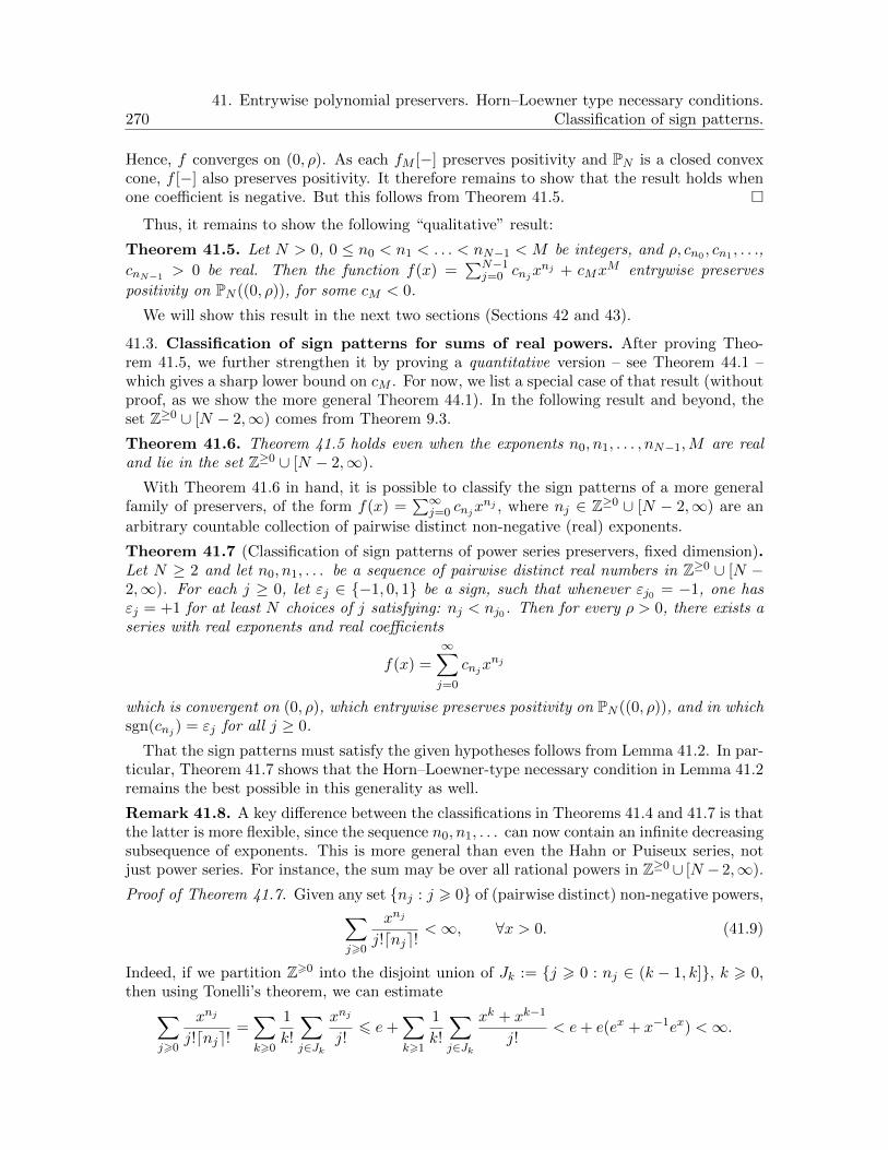
27041. Entrywise polynomial preservers. Horn–Loewner type necessary conditions.

Classification of sign patterns.

Hence, f converges on (0, ρ). As each fM [−] preserves positivity and PN is a closed convexcone, f [−] also preserves positivity. It therefore remains to show that the result holds whenone coefficient is negative. But this follows from Theorem 41.5.

Thus, it remains to show the following “qualitative” result:

Theorem 41.5. Let N > 0, 0 ≤ n0 < n1 < . . . < nN−1 < M be integers, and ρ, cn0 , cn1 , . . .,

cnN−1 > 0 be real. Then the function f(x) =∑N−1

j=0 cnjxnj + cMx

M entrywise preserves

positivity on PN ((0, ρ)), for some cM < 0.

We will show this result in the next two sections (Sections 42 and 43).

41.3. Classification of sign patterns for sums of real powers. After proving Theo-rem 41.5, we further strengthen it by proving a quantitative version – see Theorem 44.1 –which gives a sharp lower bound on cM . For now, we list a special case of that result (withoutproof, as we show the more general Theorem 44.1). In the following result and beyond, theset Z≥0 ∪ [N − 2,∞) comes from Theorem 9.3.

Theorem 41.6. Theorem 41.5 holds even when the exponents n0, n1, . . . , nN−1,M are realand lie in the set Z≥0 ∪ [N − 2,∞).

With Theorem 41.6 in hand, it is possible to classify the sign patterns of a more generalfamily of preservers, of the form f(x) =

∑∞j=0 cnjx

nj , where nj ∈ Z≥0 ∪ [N − 2,∞) are an

arbitrary countable collection of pairwise distinct non-negative (real) exponents.

Theorem 41.7 (Classification of sign patterns of power series preservers, fixed dimension).Let N ≥ 2 and let n0, n1, . . . be a sequence of pairwise distinct real numbers in Z≥0 ∪ [N −2,∞). For each j ≥ 0, let εj ∈ −1, 0, 1 be a sign, such that whenever εj0 = −1, one hasεj = +1 for at least N choices of j satisfying: nj < nj0. Then for every ρ > 0, there exists aseries with real exponents and real coefficients

f(x) =

∞∑j=0

cnjxnj

which is convergent on (0, ρ), which entrywise preserves positivity on PN ((0, ρ)), and in whichsgn(cnj ) = εj for all j ≥ 0.

That the sign patterns must satisfy the given hypotheses follows from Lemma 41.2. In par-ticular, Theorem 41.7 shows that the Horn–Loewner-type necessary condition in Lemma 41.2remains the best possible in this generality as well.

Remark 41.8. A key difference between the classifications in Theorems 41.4 and 41.7 is thatthe latter is more flexible, since the sequence n0, n1, . . . can now contain an infinite decreasingsubsequence of exponents. This is more general than even the Hahn or Puiseux series, notjust power series. For instance, the sum may be over all rational powers in Z≥0 ∪ [N − 2,∞).

Proof of Theorem 41.7. Given any set nj : j > 0 of (pairwise distinct) non-negative powers,∑j>0

xnj

j!dnje!<∞, ∀x > 0. (41.9)

Indeed, if we partition Z>0 into the disjoint union of Jk := j > 0 : nj ∈ (k − 1, k], k > 0,then using Tonelli’s theorem, we can estimate∑

j>0

xnj

j!dnje!=∑k>0

1

k!

∑j∈Jk

xnj

j!6 e+

∑k>1

1

k!

∑j∈Jk

xk + xk−1

j!< e+ e(ex + x−1ex) <∞.

41. Entrywise polynomial preservers. Horn–Loewner type necessary conditions.Classification of sign patterns. 271

We now turn to the proof. Set J := j : εj = −1 ⊂ Z≥0. By the hypotheses, for eachl ∈ J there exist j1(l), . . . , jN (l), such that εjk(l) = 1 and njk(l) < nl, for k = 1, . . . , N . Define

fl(x) :=

N∑k=1

xnjk(l)

dnjk(l)e!− δl

xnl

dnle!,

where δl ∈ (0, 1) is chosen, such that fl[−] preserves positivity on PN ((0, ρ)) by Theorem 41.6.Let J ′ ⊂ Z≥0 consist of all j > 0, such that εj = +1 but j 6= jk(l) for any l ∈ J, k ∈ [1, N ].Finally, define

f(x) :=∑l∈J

fl(x)

l!+∑j∈J ′

xnj

j!dnje!, x > 0.

Repeating the calculation in (41.9), one can verify that f converges absolutely on (0,∞) andhence on (0, ρ). By the above hypotheses and the Schur product theorem, it follows thatf [−] preserves positivity on PN ((0, ρ)).

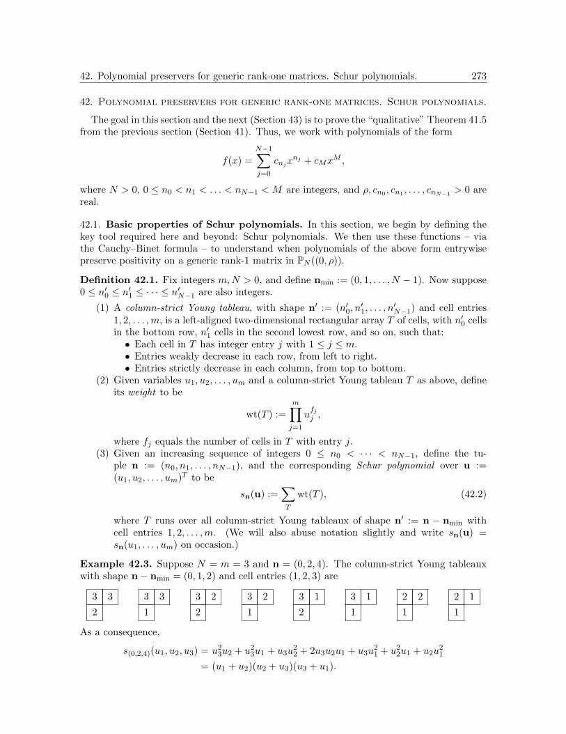
42. Polynomial preservers for generic rank-one matrices. Schur polynomials. 273

42. Polynomial preservers for generic rank-one matrices. Schur polynomials.

The goal in this section and the next (Section 43) is to prove the “qualitative” Theorem 41.5from the previous section (Section 41). Thus, we work with polynomials of the form

f(x) =

N−1∑j=0

cnjxnj + cMx

M ,

where N > 0, 0 ≤ n0 < n1 < . . . < nN−1 < M are integers, and ρ, cn0 , cn1 , . . . , cnN−1 > 0 arereal.

42.1. Basic properties of Schur polynomials. In this section, we begin by defining thekey tool required here and beyond: Schur polynomials. We then use these functions – viathe Cauchy–Binet formula – to understand when polynomials of the above form entrywisepreserve positivity on a generic rank-1 matrix in PN ((0, ρ)).

Definition 42.1. Fix integers m,N > 0, and define nmin := (0, 1, . . . , N − 1). Now suppose0 ≤ n′0 ≤ n′1 ≤ · · · ≤ n′N−1 are also integers.

(1) A column-strict Young tableau, with shape n′ := (n′0, n′1, . . . , n

′N−1) and cell entries

1, 2, . . . ,m, is a left-aligned two-dimensional rectangular array T of cells, with n′0 cellsin the bottom row, n′1 cells in the second lowest row, and so on, such that:• Each cell in T has integer entry j with 1 ≤ j ≤ m.• Entries weakly decrease in each row, from left to right.• Entries strictly decrease in each column, from top to bottom.

(2) Given variables u1, u2, . . . , um and a column-strict Young tableau T as above, defineits weight to be

wt(T ) :=

m∏j=1

ufjj ,

where fj equals the number of cells in T with entry j.(3) Given an increasing sequence of integers 0 ≤ n0 < · · · < nN−1, define the tu-

ple n := (n0, n1, . . . , nN−1), and the corresponding Schur polynomial over u :=(u1, u2, . . . , um)T to be

sn(u) :=∑T

wt(T ), (42.2)

where T runs over all column-strict Young tableaux of shape n′ := n − nmin withcell entries 1, 2, . . . ,m. (We will also abuse notation slightly and write sn(u) =sn(u1, . . . , um) on occasion.)

Example 42.3. Suppose N = m = 3 and n = (0, 2, 4). The column-strict Young tableauxwith shape n− nmin = (0, 1, 2) and cell entries (1, 2, 3) are

3 3

2

3 3

1

3 2

2

3 2

1

3 1

2

3 1

1

2 2

1

2 1

1

As a consequence,

s(0,2,4)(u1, u2, u3) = u23u2 + u2

3u1 + u3u22 + 2u3u2u1 + u3u

21 + u2

2u1 + u2u21

= (u1 + u2)(u2 + u3)(u3 + u1).

274 42. Polynomial preservers for generic rank-one matrices. Schur polynomials.

Remark 42.4. A visible notational distinction with the literature is that column-strict Youngtableaux traditionally have entries that are increasing down columns, and weakly increasingas one moves across rows. Since we only work with sets of tableaux through the sums oftheir weights occurring in Schur polynomials, this distinction is unimportant in the text, forthe following reason: define an involutive bijection ι : j 7→ m + 1 − j, where 1, . . . ,m isthe alphabet of possible cell entries. Then the column-strict Young tableaux in our notationbijectively correspond under ι – applied to each cell entry – to the “usual” column-strict Youngtableaux (in the literature); and as Schur polynomials are symmetric under permuting thevariables by ι (see Proposition 42.6), the sums of weights of the two sets of tableaux coincide.

Remark 42.5. Schur polynomials are fundamental objects in type A representation theory(of the general linear group, or the special linear Lie algebra), and are characters of irreduciblefinite-dimensional polynomial representations (over fields of characteristic zero). The aboveexample 42.3 is a special case, corresponding to the adjoint representation for the Lie algebraof 3× 3 traceless matrices. This interpretation will not be used in this text.

Schur polynomials are always homogeneous – and also symmetric, because they can bewritten as a quotient of two generalized Vandermonde determinants. This is Cauchy’s defi-nition; the definition (42.2) using Young tableaux is by Littlewood. One can show that thesetwo definitions are equivalent, among other basic properties:

Proposition 42.6. Fix integers m = N > 0 and 0 ≤ n0 < n1 < · · · < nN−1.

(1) (Cauchy’s definition.) If F is a field and u = (u1, . . . , uN )T ∈ FN , then

det(un0 | un1 | . . . | unN−1)N×N = V (u)sn(u),

where for a (column) vector or (row) tuple u, we denote by V (u) :=∏

1≤j<k≤N (uk −uj) the Vandermonde determinant as in (17.4). In particular, sn(u) is symmetric

and homogeneous of degree∑N−1

j=0 (nj − j).(2) (Principal specialization formula.) For any q ∈ F that is not a root of unity or else

has order ≥ N , we have

sn(1, q, q2, . . . , qN−1) =∏

0≤j<k≤N−1

qnk − qnjqk − qj

.

(3) (Weyl dimension formula.) Specialized to q = 1, we have

sn(1, 1, . . . , 1) =V (n)

V (nmin)∈ N.

In particular, there are V (n)/V (nmin) column-strict tableaux of shape n − nmin andcell entries 1, . . . , N . Here and below, we will mildly abuse notation and write V (n)for a tuple/row vector n to denote V (nT ).

Proof. The first part is proved in Theorem 46.1 below. Using this, we show the second part.Set u := (1, q, q2, . . . , qN−1)T with q as given. Then it is easy to verify that

sn(u) =det(un0 | un1 | . . . | unN−1)

V (u)=V ((qn0 , . . . , qnN−1))

V ((q0, . . . , qN−1))=

∏0≤j<k≤N−1

qnk − qnjqk − qj

,

as desired.Finally, to prove the Weyl dimension formula, notice that by the first part, the Schur

polynomial has integer coefficients and hence makes sense over Z, and then specializes

42. Polynomial preservers for generic rank-one matrices. Schur polynomials. 275

to sn(u) over any ground field. Now work over the ground field Q, and let fn(T ) :=sn(1, T, . . . , TN−1) ∈ Z[T ] be the corresponding “principally specialized” polynomial. Then,

V ((q0, . . . , qN−1))fn(q) = V ((qn0 , . . . , qnN−1)), ∀q ∈ Q.

In particular, for every q 6= 1, dividing both sides by (q − 1)(N2 ), we obtain:∏

0≤j<k≤N−1

(qnj + qnj+1 + · · ·+ qnk−1)− fn(q)∏

0≤j<k≤N−1

(qj + qj+1 + · · ·+ qk−1) = 0,

for all q ∈ Q \ 1. This means that the left-hand side is (the specialization of) a polynomialwith infinitely many roots, hence the polynomial vanishes identically on Q. Specializing thispolynomial to q = 1 now yields the Weyl dimension formula

V (n)

V (nmin)=

∏0≤j<k≤N−1

nk − njk − j

= fn(1) = sn(1, . . . , 1).

The final assertion now follows from Littlewood’s definition (42.2) of sn(u).

42.2. Polynomials preserving positivity on individual rank-one positive matrices.We return to proving Theorem 41.5, and hence Theorem 41.4 on sign patterns. As we haveshown, it suffices to prove the theorem for one higher degree (leading) term with a negativecoefficient. Before proving the result in full, we tackle the following (simpler) versions. Thus,

we are given a real polynomial as above: f(x) =∑N−1

j=0 cnjxnj + cMx

M , where cnj > 0 ∀j.(1) Does there exist cM < 0, such that f [−] : PN ((0, ρ))→ PN?

Here is a reformulation: dividing the expression for f(x) throughout by |cM | =1/t > 0, define

pt(x) := tN−1∑j=0

cnjxnj − xm, where cnj > 0 ∀j. (42.7)

Then it is enough to ask for which t > 0 (if any) does pt[−] : PN ((0, ρ))→ PN?(2) Here are two simplifications: Can we produce such a constant t > 0 for only the

subset of rank-1 matrices in PN ((0, ρ))? How about for a single rank-1 matrix uuT ?(3) A further special case: let u be generic, in that u ∈ (0, ρ)N has distinct coordinates,

and pt is as above. Can one now compute all t > 0, such that pt[uuT ] ∈ PN? Howabout all t > 0, such that det pt[uuT ] ≥ 0?

We begin by answering the last of these questions – the answer crucially uses Schur poly-nomials. The following result shows that, in fact, det pt[uuT ] ≥ 0 implies pt[uuT ] is positivesemidefinite!

Proposition 42.8. With N ≥ 1 and notation as in (42.7), define the vectors

n := (n0, . . . , nN−1), nj := (n0, . . . , nj−1, nj , nj+1, . . . , nN−1,M), 0 ≤ j < N, (42.9)

where 0 ≤ n0 < · · · < nN−1 < M . Now if the nj and M are integers, and a vector u ∈ (0,∞)N

has pairwise distinct coordinates, then the following are equivalent:

(1) pt[uuT ] is positive semidefinite.(2) det pt[uuT ] ≥ 0.

(3) t ≥N−1∑j=0

snj (u)2

cnjsn(u)2.

276 42. Polynomial preservers for generic rank-one matrices. Schur polynomials.

In particular, at least for “most” rank-1 matrices, it is possible to find polynomial preserversof positivity (on that one matrix), with a negative coefficient.

The proof of Proposition 42.8 uses the following even more widely applicable equivalencebetween the non-negativity of the determinant and of the entire spectrum for “special” linearpencils of matrices:

Lemma 42.10. Fix w ∈ RN and a positive definite matrix H. Define the linear pencilPt := tH −wwT , for t > 0. Then the following are equivalent:

(1) Pt is positive semidefinite.(2) detPt ≥ 0.

(3) t ≥ wTH−1w = 1− det(H −wwT )

detH.

This lemma is naturally connected to the theory of (generalized) Rayleigh quotients, al-though we do not pursue this further.

Proof. We show a cyclic chain of implications. That (1) =⇒ (2) is immediate.

(2) =⇒ (3) : Using the identity (2.33) from Section 2.4 on Schur complements, we obtainby taking determinants

det

(A BB′ D

)= detD · det(A−BD−1B′)

whenever A,D are square matrices, with D invertible. Using this, we compute:

0 ≤ det(tH −wwT ) = det

(tH wwT 1

)= det

(1 wT

w tH

)= det(tH) det(1−wT (tH)−1w).

Since the last quantity is a scalar, and det(tH) > 0 by assumption, it follows from (2) that

1 ≥ t−1(wTH−1w) =⇒ t ≥ wTH−1w.

Now substitute t = 1 in the above computation, to obtain

det(H −wwT ) = det(H) det(1−wTH−1w)

=⇒ det(H −wwT )

detH= 1−wTH−1w ≥ 1− t,

which implies (3).

(3) =⇒ (1) : It suffices to show that xTPtx ≥ 0 for all non-zero vectors x ∈ RN . Using a

change of variables y =√Hx 6= 0, we compute:

xTPtx = tyTy − (yT√H−1

w)2

= ‖y‖2(t− ((y′)T√H−1

w)2), where y′ :=y

‖y‖

≥ ‖y‖2(t− ‖y′‖2∥∥∥√H−1w

∥∥∥2) (using Cauchy–Schwarz)

= ‖y‖2(t−wTH−1w) ≥ 0 (by assumption).

We can now answer the last of the above questions on positivity preservers, for genericrank-1 matrices.

42. Polynomial preservers for generic rank-one matrices. Schur polynomials. 277

Proof of Proposition 42.8. The result is easily shown for N = 1, so we now assume N ≥ 2.We are interested in the following matrix and its determinant:

pt[uuT ] = tN−1∑j=0

cnj (unj )(unj )T − (uM )(uM )T .

We first work more generally: over any field F, and with matrices uvT , where u,v ∈ FN .Thus, we study

pt[uvT ] = tN−1∑j=0

cnjunj (vnj )T − uM (vM )T ,

where t, cnj ∈ F, and cnj 6= 0 ∀j. Setting D = diag(tcn0 , . . . , tcnN−1 ,−1), we have thedecomposition

pt[uvT ] = U(u)DU(v)T , where U(u)N×(N+1) := (un0 | . . . | unN−1 | uM ).

Applying the Cauchy–Binet formula to A = U(u), B = DU(v)T , as well as Cauchy’s defini-tion in Proposition 42.6(1), we obtain the following general determinantal identity, valid overany field:

det pt[uvT ] = V (u)V (v)tN−1N−1∏j=0

cnj ·

sn(u)sn(v)t−N−1∑j=0

snj (u)snj (v)

cnj

. (42.11)

Now specialize this identity to F = R, with t, cnj > 0 and u = v ∈ (0,∞)N having distinctcoordinates. From this we deduce the following consequences. First, set

H :=

N−1∑j=0

cnj (uuT )nj = U ′(u)D′U ′(u)T , w := uM ,

whereD′ := diag(cn0 , . . . , cnN−1) is a positive definite matrix and U ′(u) := (un0 | . . . | unN−1)is a generalized Vandermonde matrix which has determinant V (u)sn(u) 6= 0. From this itfollows that H is positive definite, so Lemma 42.10 applies. Moreover, H −wwT = p1[uuT ],so using the above calculation (42.11) and the Cauchy–Binet formula respectively, we have

det(H −wwT ) = V (u)2N−1∏j=0

cnj · sn(u)2

1−N−1∑j=0

snj (u)2

cnjsn(u)2

,

detH = V (u)2N−1∏j=0

cnj · sn(u)2.

In particular, from Lemma 42.10(3) we obtain

wTH−1w =N−1∑j=0

snj (u)2

cnjsn(u)2.

Now the proposition follows directly from Lemma 42.10, since Pt = pt[uuT ] for all t > 0.

43. First-order approximation / leading term of Schur polynomials.From rank-one matrices to all matrices. 279

43. First-order approximation / leading term of Schur polynomials. Fromrank-one matrices to all matrices.

In the previous section, we computed the exact threshold for the leading term of a poly-nomial

pt(x) := tN−1∑j=0

cnjxnj − xM , where cnj > 0 ∀j

(and where 0 ≤ n0 < · · · < nN−1 < M are integers), such that pt[uuT ] ∈ PN for a singlevector u ∈ (0,∞)N with pairwise distinct coordinates. Recall that our (partial) goal is tofind a threshold that works for all rank-1 matrices uuT ∈ PN ((0, ρ)) – i.e., for u ∈ (0,

√ρ)N .

Thus, we need to show that the supremum of the threshold over all such u is bounded:

supu∈(0,

√ρ)N

N−1∑j=0

snj (u)2

cnjsn(u)2<∞.

Since we only consider vectors u with positive coordinates, it suffices to bound snj (u)/sn(u)from above, for each j. In turn, for this it suffices to find lower and upper bounds for everySchur polynomial evaluated at u ∈ (0,∞)N . This is achieved by the following result:

Theorem 43.1 (First-order approximation/Leading term of Schur polynomials). Say N ≥ 1and 0 ≤ n0 < · · · < nN−1 are integers. Then for all real numbers 0 < u1 ≤ u2 ≤ · · · ≤ uN ,we have the bounds

1× un−nmin ≤ sn(u) ≤ V (n)

V (nmin)× un−nmin ,

where un−nmin = un0−01 un1−1

2 · · ·unN−1−(N−1)N and V (n) is as in (17.4). Moreover, the con-

stants 1 and V (n)V (nmin) cannot be improved.

Proof. Recall that sn(u) is obtained by summing the weights of all column-strict Youngtableaux of shape n − nmin with cell entries 1, . . . , N . Moreover, by the Weyl dimensionformula in Proposition 42.6(3), there are precisely V (n)/V (nmin) such tableaux. Now eachsuch tableau can have weight at most un−nmin , as follows: the cells in the top row each haveentries at most N ; the cells in the next row at most N − 1; and so on. The tableau Tmax

obtained in this fashion has weight precisely un−nmin . Hence, by definition, we have

un−nmin = wt(Tmax) ≤∑T

wt(T ) = sn(u) ≤∑T

wt(Tmax) =V (n)

V (nmin)un−nmin .

This proves the bounds; we claim that both bounds are sharp. If n = nmin then all terms inthe claimed inequalities are 1, and we are done. Thus, assume henceforth that n 6= nmin. LetA > 1 and define u(A) := (A,A2, . . . , AN ). Then wt(Tmax) = AM for some M > 0. Hence,for every column-strict Young tableau T 6= Tmax as above, wt(T ) is at most wt(Tmax)/A andat least 1 = wt(Tmax)/AM . Now summing over all such tableaux T yields

sn(u(A)) ≤ u(A)n−nmin

(1 +

(V (n)

V (nmin)− 1

)1

A

),

sn(u(A)) ≥ u(A)n−nmin

(1 +

(V (n)

V (nmin)− 1

)1

AM

).

Divide throughout by u(A)n−nmin ; now taking the limit as A→∞ yields the sharp lowerbound 1 while taking the limit as A→ 1+ yields the sharp upper bound V (n)/V (nmin).

28043. First-order approximation / leading term of Schur polynomials.

From rank-one matrices to all matrices.

We now use Theorem 43.1, and Proposition 42.8 in the previous section, to find a thresholdfor t > 0 beyond which pt[−] preserves positivity on all rank-1 matrices in PN ((0, ρ)) – and,in fact, on all matrices in PN ((0, ρ)).

Theorem 43.2. Fix integers N ≥ 1, 0 ≤ n0 < n1 < · · · < nN−1 < M , and scalars

ρ, t, cn0 , . . . , cnN−1 > 0. The polynomial pt(x) := t∑N−1

j=0 cnjxnj − xM entrywise preserves

positivity on PN ((0, ρ)), if t ≥ t0 :=N−1∑j=0

V (nj)2

cnjV (nmin)2ρM−nj .

The notation in Definition 25.1 is useful here and in the sequel. Specifically, XN,6= for a setX and an integer N ≥ 1 denotes the set of N -tuples from X with pairwise distinct entries.

Proof of Theorem 43.2. Given u ∈ (0,√ρ)N,6=, from Proposition 42.8 it follows that pt[uuT ] ∈

PN if and only if t ≥∑N−1

j=0

snj (u)2

cnj sn(u)2. Now suppose u ∈ (0,

√ρ)N,↑. Then by Theorem 43.1,

N−1∑j=0

snj (u)2

cnjsn(u)2≤

N−1∑j=0

u2(nj−nmin)V (nj)2/V (nmin)2

cnju2(n−nmin)

=N−1∑j=0

V (nj)2

cnjV (nmin)2u2(nj−n),

and this is bounded above by t0, since if v :=√ρ(1, . . . , 1)T then u2(nj−n) ≤ v2(nj−n) =

ρM−nj for all j. Thus, we conclude that

t ≥ t0 =⇒ pt[uuT ] ∈ PN ∀u ∈ (0,√ρ)N,↑ =⇒ pt[uuT ] ∈ PN ∀u ∈ (0,

√ρ)N,6=

=⇒ pt[uuT ] ∈ PN ∀u ∈ (0,√ρ)N ,

where the first implication was proved above, the second follows by (the symmetric nature ofSchur polynomials and by) relabeling the rows and columns of uuT to rearrange the entriesof u in increasing order, and the third implication follows from the continuity of pt and the

density of (0,√ρ)N,6= in (0,

√ρ)N .

This validates the claimed threshold t0 for all rank-1 matrices. To prove the result on allof PN ((0, ρ)), we use induction on N ≥ 1, with the base case of N = 1 already done since1× 1 matrices have rank 1.

For the induction step, recall the extension principle (Theorem 9.12), which said that:Suppose I = (0, ρ) or (−ρ, ρ) or its closure, for some 0 < ρ ≤ ∞. If h ∈ C1(I) is such thath[−] preserves positivity on rank-1 matrices in PN (I) and h′[−] : PN−1(I) → PN−1, thenh[−] : PN (I)→ PN .

We will apply this result to h(x) = pt0(x), with t0 as above. By the extension principle,we need to show that h′[−] : PN−1((0, ρ))→ PN−1. Note that

h′(x) = t0

N−1∑j=0

njcnjxnj−1 −MxM−1 = Mg(x) + t0n0cn0x

n0−1,

where we define

g(x) :=t0M

N−1∑j=1

njcnjxnj−1 − xM−1.

We claim that the entrywise polynomial map g[−] : PN−1((0, ρ)) → PN−1. If this holds,then by the Schur product theorem, the same property is satisfied by Mg(x) + t0n0cn0x

n0−1

(regardless of whether n0 = 0 or n0 > 0). But this function is precisely h′ and the theoremwould follow.

43. First-order approximation / leading term of Schur polynomials.From rank-one matrices to all matrices. 281

It thus remains to prove the claim, and we do so via a series of reductions and simplifications– i.e., “working backward”. By the induction hypothesis, Theorem 43.2 holds in dimensionN − 1 ≥ 1, for the polynomials

qt(x) := t

N−1∑j=1

njcnjxnj−1 − xM−1.

For this family, the threshold is now given by

N−1∑j=1

V (n′j)2

njcnjV (n′min)2ρM−1−(nj−1),

where

n′min := (0, 1, . . . , N − 2), n′j := (n1, . . . , nj−1, nj , nj+1, . . . , nN−1,M) ∀j > 0.

Thus, the proof is complete if we show that

N−1∑j=1

V (n′j)2

njcnjV (n′min)2ρM−1−(nj−1) ≤ t0

M=

N−1∑j=0

V (nj)2

McnjV (nmin)2ρM−nj .

In turn, comparing just the jth summand for each j > 0, it suffices to show that

V (n′j)√njV (n′min)

≤ V (nj)√MV (nmin)

, ∀j > 0.

Dividing the right-hand side by the left-hand side, and canceling common factors, we obtainthe expression

N−1∏k=1

nk − n0

k·√nj√M· M − n0

nj − n0.

Since every factor in the product term is at least 1, it remains to show that

M − n0

nj − n0≥√M√nj, ∀j > 0.

But this follows from a straightforward calculation:

(M − n0)2nj − (nj − n0)2M = (M − nj)(Mnj − n20) > 0,

and the proof is complete.

Finally, we recall our original goal of classifying the sign patterns of positivity preserversin a fixed dimension – see Theorem 41.4. We showed this result holds if one can prove itsspecial case, Theorem 41.5. Now this latter result follows from Theorem 43.2, by setting

cM := −t−10 , where t0 =

N−1∑j=0

V (nj)2

cnjV (nmin)2ρM−nj as in Theorem 43.2.

44. Exact quantitative bound: monotonicity of Schur ratios.Real powers and power series. 283

44. Exact quantitative bound: monotonicity of Schur ratios. Real powersand power series.

In the last two sections (Sections 42 and 43), we proved the existence of a negative thresholdcM for polynomials

f(x) =

N−1∑j=0

cnjxnj + cMx

M

to entrywise preserve positivity on PN ((0, ρ)). (Here N > 0 and 0 ≤ n0 < · · · < nN−1 < Mare integers.) We now compute the exact value of this threshold, more generally for realpowers; this has multiple consequences which are described after stating Theorem 44.1. Thus,our goal is to prove the following quantitative result, for real powers – including negativepowers:

Theorem 44.1. Fix an integer N > 0 and real powers n0 < · · · < nN−1 < M . Also fix realscalars ρ > 0 and cn0 , . . . , cnN−1 , cM , and define

f(x) :=N−1∑j=0

cnjxnj + cMx

M . (44.2)

Then the following are equivalent:

(1) The entrywise map f [−] preserves positivity on all rank-1 matrices in PN ((0, ρ)).(2) The map f [−] preserves positivity on rank-1 totally non-negative (TN) Hankel ma-

trices in PN ((0, ρ)).(3) Either all cnj , cM > 0; or cnj > 0 ∀j and cM > −C−1, where

C =N−1∑j=0

V (nj)2

cnjV (n)2ρM−nj . (44.3)

Here V (u),n,nj are defined as in (17.4) and (42.9).

If, moreover, we assume that nj ∈ Z>0 ∪ [N − 2,∞) for all j, then the above conditions arefurther equivalent to the “full-rank” version:

(4) The entrywise map f [−] preserves positivity on PN ([0, ρ]), where we set 00 := 1.

Theorem 44.1 is a powerful result. It has multiple applications; we now list some of them.

(1) Suppose M = N and nj = j for 0 ≤ j ≤ N − 1. Then the result provides a completecharacterization of which polynomials of degree ≤ N entrywise preserve positivity onPN ((0, ρ)) – or more generally, on any intermediate set between PN ((0, ρ)) and therank-1 Hankel TN matrices inside it.

(2) In fact, a similar result to the previous characterization is implied, whenever oneconsiders linear combinations of at most N + 1 monomial powers.

(3) The result provides information on positivity preservers beyond polynomials, sincenj ,M are now allowed to be real, even negative if one works with rank-1 matrices.

(4) In particular, the result implies Theorem 41.6, and hence Theorem 41.7 (see its proof).This latter theorem provides a full classification of the sign patterns of possible “count-able sums of real powers” which entrywise preserve positivity on PN ((0, ρ)).

(5) The result also provides information on preservers of total non-negativity on Hankelmatrices in fixed dimension; see Corollary 44.11.

28444. Exact quantitative bound: monotonicity of Schur ratios.

Real powers and power series.

(6) There are further applications, two of which are (i) to the matrix cube problem and tosharp linear matrix inequalities/spectrahedra involving entrywise powers; and (ii) tocomputing the simultaneous kernels of entrywise powers and a related “Schubert cell-type” stratification of the cone PN (C). These are explained in the 2016 paper ofBelton, Guillot, Khare, and Putinar in Adv. in Math.; see also the 2021 paper inAmer. J. Math. by Khare and Tao (mentioned a few lines above (41.1)).

(7) Theorem 44.1 is proved using a monotonicity phenomenon for ratios of Schur poly-nomials; see Theorem 44.6. This latter result is also useful in extending a 2011conjecture by Cuttler–Greene–Skandera (and its proof). In fact, this line of attackends up characterizing majorization and weak majorization – for real tuples – usingSchur polynomials. See the aforementioned paper by Khare and Tao [217] for moredetails.

(8) One further application is Theorem 44.14, which finds a threshold for bounding by∑N−1j=0 cnjA

nj , any power series – and more general “Laplace transforms” – appliedentrywise to a positive matrix A. This extends Theorem 44.1, where the powerseries is simply xM , because Theorem 44.1 says in particular that (xM )[A] = AM is

dominated by a multiple of∑N−1

j=0 cnjAnj .

(9) As mentioned in the remarks prior to Theorem 41.4, Theorem 44.1 also providesexamples of power series preservers on PN ((0, ρ)) with negative coefficients; and ofsuch functions which preserve positivity on PN ((0, ρ)) but not on PN+1((0, ρ)).

44.1. Monotonicity of ratios of Schur polynomials. The proof of Theorem 44.1 usesthe same ingredients as developed in previous sections. A summary of what follows is nowprovided. In the rank-1 case, we use a variant of Proposition 42.8 for an individual matrix;the result does not apply as is, since the powers may now be real. Next, in order to find thesharp threshold for all rank-1 matrices, even for real powers we crucially appeal to the integerpower case. Namely, we will first understand the behavior and supremum of the functionsnj (u)/sn(u) over u ∈ (0,

√ρ)N (and for each 0 ≤ j ≤ N − 1). One may hope that these

suprema behave well enough that the sharp threshold can be computed for rank-1 matrices;the further hope would be that this threshold bound is tight enough to behave well withrespect to the extension principle in Theorem 9.12, and hence to work for all matrices inPN ((0, ρ)). Remarkably, these two hopes are indeed justified, proving the theorem.

We begin with the key result required to be able to take suprema over ratios of Schurpolynomials sm(u)/sn(u). To motivate the result, here is a special case.

Example 44.4. Suppose N = 3,n = (0, 2, 3), and m = (0, 2, 4). As above, we have u =

(u1, u2, u3)T and nmin = (0, 1, 2). Now let f(u) := sm(u)sn(u) : (0,∞)N → (0,∞). This is a

rational function, whose numerator sums weights over tableaux of shape (0, 1, 2), and henceby Example 42.3 above, equals (u1 + u2)(u2 + u3)(u3 + u1). The denominator sums weightsover tableaux of shape (0, 1, 1); there are only three such tableaux

3

2

3

1

2

1

and hence,

f(u) :=(u1 + u2)(u2 + u3)(u3 + u1)

u1u2 + u2u3 + u3u1, u1, u2, u3 > 0.

Notice that the numerator and denominator are both Schur polynomials, hence positivecombinations of monomials (this is called “monomial positivity”). In particular, they are both

44. Exact quantitative bound: monotonicity of Schur ratios.Real powers and power series. 285

non-decreasing in each coordinate. One can verify that their ratio f(u) is not a polynomial;moreover, it is not a priori clear if f(u) shares the same coordinatewise monotonicity property.However, we claim that this does hold, i.e., f(u) is non-decreasing in each coordinate onu ∈ (0,∞)N .

To see why: by symmetry, it suffices to show that f is non-decreasing in u3. Using thequotient rule of differentiation, we claim that the expression

sn(u)∂u3sm(u)− sm(u)∂u3sn(u) (44.5)

is non-negative on (0,∞)3. Indeed, computing this expression yields

(u1 + u2)(u1u3 + 2u1u2 + u2u3)u3,

and this is clearly non-negative, as desired. More strongly, the expression (44.5) turns out tobe monomial positive, which implies non-negativity.

Here is the punchline: an even stronger phenomenon holds. Namely, when we write the

expression (44.5) in the form∑

j≥0 pj(u1, u2)uj3, each polynomial pj is Schur positive! Thismeans that it is a non-negative integer-linear combination of Schur polynomials:

p0(u1, u2) = 0,

p1(u1, u2) = 2u1u22 + 2u2

1u2 = 22 2

1+ 2

2 1

1= 2s(1,3)(u1, u2),

p2(u1, u2) = (u1 + u2)2 = 2 2 + 2 1 + 1 1 + 2

1= s(0,3)(u1, u2) + s(1,2)(u1, u2),

modulo a mild abuse of notation. This yields the sought-for non-negativity, as each sn(u)is monomial positive by definition. (See the discussion following (30.16) for the “original”occurrence of monomial positivity and its “upgrade” to (skew) Schur positivity.)

The remarkable fact is that the phenomena described in the above example also occur forevery pair of Schur polynomials sm(u), sn(u) for which m ≥ n coordinatewise:

Theorem 44.6 (Monotonicity of Schur polynomial ratios). Suppose 0 6 n0 < · · · < nN−1

and 0 6 m0 < · · · < mN−1 are integers satisfying: nj 6 mj ∀j. Then the symmetric function

f : (0,∞)N → R, f(u) :=sm(u)

sn(u)

is non-decreasing in each coordinate.More strongly, viewing the expression

sn(u) · ∂uN sm(u)− sm(u) · ∂uN sn(u)

as a polynomial in uN , the coefficient of each monomial ujN is a Schur positive polynomial in

(u1, u2, . . . , uN−1)T .

Theorem 44.6 is an application of a deep result in representation theory/symmetric functiontheory, by Lam, Postnikov, and Pylyavskyy in Amer. J. Math. (2007). The proof of thislatter result is beyond the scope of this text, and hence is not pursued further; but its usagemeans that in the spirit of the previous two sections, the proof of Theorem 44.6 once againcombines analysis with symmetric function theory. Moreover, this 2007 result in [231] arosefrom the prior work of Skandera [338] in 2004, on determinant inequalities for minors oftotally non-negative matrices.

To proceed further, we introduce the following notation:

28644. Exact quantitative bound: monotonicity of Schur ratios.

Real powers and power series.

Definition 44.7. Given a vector u = (u1, . . . , um)T ∈ (0,∞)m and a real tuple n =(n0, . . . , nN−1) for integers m,N ≥ 1, define

un := (un0 | . . . | unN−1)m×N = (unk−1

j )m,Nj=1,k=1.

We now extend Theorem 44.6 to arbitrary real powers (instead of non-negative integerpowers). As one can no longer use Schur polynomials, the next result uses generalized Van-dermonde determinants instead:

Theorem 44.8. Fix an integer N ≥ 1 and real tuples

n = (n0 < n1 < · · · < nN−1), m = (m0 < m1 < · · · < mN−1)

with nj ≤ mj ∀j and n 6= m. Then the symmetric function

f6=(u) :=det(um)

det(un)

is non-decreasing in each coordinate on (0,∞)N, 6=. (See Definition 25.1.)

Proof. The result is immediate for N = 1; henceforth suppose N ≥ 2. For a fixed t ∈ R, iffor each j we multiply the jth row of the matrix um by utj , we obtain a matrix um

′where

m′j = mj + t ∀j. In particular, if we start with real powers nj ,mj , then multiplying the

numerator and denominator of f6= by (u1 · · ·uN )−n0 reduces the situation to working with

the non-negative real tuples n′ := (nj − n0)N−1j=0 and m′ := (mj − n0)N−1

j=0 . Thus, we supposehenceforth that nj ,mj ≥ 0 ∀j.

If nj ,mj are all integers, then the result is an immediate reformulation of the first part ofTheorem 44.6, via Proposition 42.6(1). Next suppose nj ,mj are rational. Choose a (large)

integer L > 0 such that Lnj , Lmj ∈ Z ∀j and define yj := u1/Lj . By the previous subcase,

the symmetric function

f(y) :=det(yLm)

det(yLn)=

det(um)

det(un), y := (y1, . . . , yN )T ∈ (0,∞)N, 6=

is coordinatewise non-decreasing on (0,∞)N, 6= in the yj , and hence on (0,∞)N,6= in the uj .Finally, in the general case, given non-negative real powers nj ,mj satisfying the hypotheses,

choose sequences

0 ≤ n0,k < n1,k < · · · < nN−1,k, 0 ≤ m0,k < m1,k < · · · < mN−1,k

for k = 1, 2, . . . , which further satisfy:

(1) nj,k,mj,k are rational for 0 ≤ j ≤ N − 1, k ≥ 1;(2) nj,k ≤ mj,k ∀j, k; and(3) nj,k → nj and mj,k → mj as k →∞, for each j = 0, 1, . . . , N − 1.

By the rational case above, for each k ≥ 1 the symmetric function

fk(u) :=det(umk)

det(unk)

is coordinatewise non-decreasing, where mk := (m0,k, . . . ,mN−1,k) and similarly for nk. Butthen their limit limk→∞ fk(u) = f6=(u) is also coordinatewise non-decreasing, as claimed.

44. Exact quantitative bound: monotonicity of Schur ratios.Real powers and power series. 287

44.2. Proof of the quantitative bound. Using Theorem 44.8, we can now prove the mainresult in this section.

Proof of Theorem 44.1. We first work only with rank-1 matrices. Clearly, (1) =⇒ (2), andwe show that (2) =⇒ (3) =⇒ (1).

If all coefficients cnj , cM ≥ 0, then f [−] preserves positivity on rank-1 matrices. Otherwise,by the Horn–Loewner-type necessary conditions in Lemma 41.2 (now for real powers, possiblynegative!), it follows that cn0 , . . . , cnN−1 > 0 > cM . In this case, the discussion that opensSection 42.2 allows us to reformulate the problem using

pt(x) := tN−1∑j=0

cnjxnj − xM , t > 0,

and the goal is to find a sharp positive lower bound for t, above which pt[−] preservespositivity on rank-1 Hankel TN matrices uuT ∈ PN ((0, ρ)).

But now one can play the same game as in Section 42.2. In other words, Lemma 42.10shows that the “real powers analogue” of Proposition 42.8 holds: pt[uuT ] ≥ 0 if and only if

t ≥N−1∑j=0

det(unj )2

cnj det(un)2,

for all generic rank-1 matrices uuT , with u ∈ (0,√ρ)N, 6=. By the same reasoning as in the

proof of Theorem 43.2 (see the previous section), pt[−] preserves positivity on a given testset of rank-1 matrices uuT : u ∈ S ⊂ (0,

√ρ)N, if and only if (by density and continuity,)

t exceeds the following supremum:

t ≥ supu∈S∩(0,

√ρ)N, 6=

N−1∑j=0

det(unj )2

cnj det(un)2. (44.9)

This is, of course, subject to S∩ (0,√ρ)N, 6= being dense in the set S, which is indeed the case

if uuT : u ∈ S ∩ (0,√ρ)N equals the set of rank-1 Hankel TN matrices as in assertion (2).

Thus, to prove (2) =⇒ (3) =⇒ (1) in the theorem, it suffices to prove: (i) the

supremum (44.9) is bounded above by the value

N−1∑j=0

V (nj)2

cnjV (n)2ρM−nj ; and (ii) this value is

attained on (a countable set of) rank-1 Hankel TN matrices, hence it equals the supremum.We now prove both of these assertions. By Theorem 44.8, each ratio det(unj )/ det(un) is

coordinatewise non-decreasing, hence its supremum on (0,√ρ)N, 6= is bounded above by (and

in fact equals) its limit as u→ √ρ(1−, . . . , 1−). To see why this limit exists, note that every

vector u ∈ (0, ρ)N is bounded above – coordinatewise – by a vector of the form

u(ε) :=√ρ(ε, ε2, . . . , εN )T ∈ (0,

√ρ)N,6=, ε ∈ (0, 1).

In particular, by Theorem 44.8 the limit as u → √ρ(1−, . . . , 1−) exists and equals the limit

by using the rank-1 Hankel TN family u(ε)u(ε)T , for any sequence of ε → 1− – providedthis latter limit exists. We show this presently; thus, we work with a countable sequence ofε→ 0+ in place of Lemma 41.2, and another countable sequence of ε→ 1− in what follows.First observe:

28844. Exact quantitative bound: monotonicity of Schur ratios.

Real powers and power series.

Lemma 44.10 (Principal specialization formula for real powers). Suppose q > 0 and n0 <n1 < · · · < nN−1 are real exponents. If n := (n0, . . . , nN−1) and u := (1, q, . . . , qN−1)T , then

det(un) =∏

0≤j<k≤N−1

(qnk − qnj ) = V (qn).

The proof is exactly the same as of Proposition 42.6(2), since the transpose of un is a usualVandermonde matrix.

We can now complete the proof of Theorem 44.1. The above lemma immediately implies

det(u(ε)nj )

det(u(ε)n)=√ρM−nj

V (εnj )

V (εn), ∀0 ≤ j ≤ N − 1.

Dividing the numerator and denominator by (1− ε)(N2 ) and taking the limit as ε→ 1− using

L’Hopital’s rule, we obtain the expression√ρM−nj

V (nj)V (n) . Since all of these suprema/limits

occur as ε→ 1−, we finally have

supu∈(0,

√ρ)N, 6=

N−1∑j=0

det(unj )2

cnj det(un)2= lim

ε→1−

N−1∑j=0

det(u(ε)nj )2

cnj det(u(ε)n)2=

N−1∑j=0

V (nj)2

V (n)2

ρM−nj

cnj.

This proves the equivalence of assertions (1)–(3) in the theorem, for rank-1 matrices.Finally, suppose all nj ∈ Z≥0 ∪ [N − 2,∞). In this case (4) =⇒ (1) is immediate. Con-

versely, given that (1) holds, we prove (4) using once again the integration trick of FitzGeraldand Horn, as isolated in Theorem 9.12. The proof and calculation are similar to that of The-orem 43.2 above and are left to the interested reader as an exercise.

44.3. Applications to Hankel TN preservers in a fixed dimension and to powerseries preservers. We conclude by discussing some applications of Theorem 44.1. First,the result implies in particular that AM is bounded above by a multiple of

∑N−1j=0 cnjA

nj .In particular, the proof of Theorem 41.7 above goes through; thus, we have classified the signpatterns of all entrywise power series preserving positivity on PN ((0, ρ)).

Second, the equivalent conditions in Theorem 44.1 classifying the (entrywise) polynomialpositivity preservers on PN ((0, ρ)) – or on rank-1 matrices – also end up classifying thepolynomial preservers of total non-negativity on the corresponding Hankel test sets:

Corollary 44.11. With notation as in Theorem 44.1, if we restrict to all real powers andonly rank-1 matrices, then assertions (1)–(3) in Theorem 44.1 are further equivalent to:

(1′) f [−] preserves total non-negativity on all rank-1 matrices in HTNN with entries in(0, ρ).

If, moreover, all nj lie in Z≥0 ∪ [N − 2,∞), then these conditions are further equivalentto:

(4′) f [−] preserves total non-negativity on all matrices in HTNN with entries in [0, ρ].

Recall here that by Definition 12.18, HTNN denotes the set of N ×N Hankel totally non-negative matrices.

Proof. Clearly, (4′) implies (1′), which implies assertion (2) in Theorem 44.1. Conversely, weclaim that assertion (1) in Theorem 44.1 implies (1′) via Theorem 4.1. Indeed, if A ∈ HTNNhas rank 1 and entries in (0, ρ), then f [A] ∈ PN by Theorem 44.1(1). Similarly, A(1)⊕(0)1×1 ∈PN ((0, ρ)) and has rank 1, so f [A(1)] is also positive semidefinite, and hence Theorem 4.1applies, as desired. The same proof works to show that (4′) follows from Theorem 44.1(4).

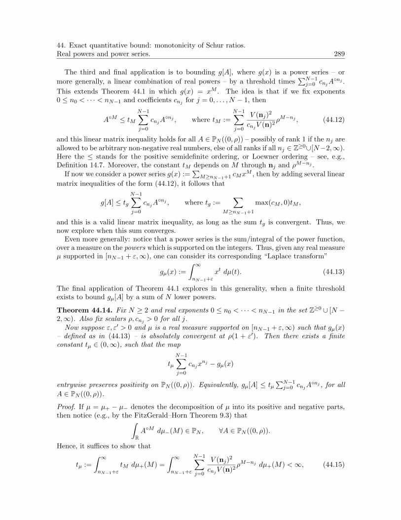
44. Exact quantitative bound: monotonicity of Schur ratios.Real powers and power series. 289

The third and final application is to bounding g[A], where g(x) is a power series – or

more generally, a linear combination of real powers – by a threshold times∑N−1

j=0 cnjAnj .

This extends Theorem 44.1 in which g(x) = xM . The idea is that if we fix exponents0 ≤ n0 < · · · < nN−1 and coefficients cnj for j = 0, . . . , N − 1, then

AM ≤ tMN−1∑j=0

cnjAnj , where tM :=

N−1∑j=0

V (nj)2

cnjV (n)2ρM−nj , (44.12)

and this linear matrix inequality holds for all A ∈ PN ((0, ρ)) – possibly of rank 1 if the nj areallowed to be arbitrary non-negative real numbers, else of all ranks if all nj ∈ Z≥0∪[N−2,∞).Here the ≤ stands for the positive semidefinite ordering, or Loewner ordering – see, e.g.,Definition 14.7. Moreover, the constant tM depends on M through nj and ρM−nj .

If now we consider a power series g(x) :=∑

M≥nN−1+1 cMxM , then by adding several linear

matrix inequalities of the form (44.12), it follows that

g[A] ≤ tgN−1∑j=0

cnjAnj , where tg :=

∑M≥nN−1+1

max(cM , 0)tM ,

and this is a valid linear matrix inequality, as long as the sum tg is convergent. Thus, wenow explore when this sum converges.

Even more generally: notice that a power series is the sum/integral of the power function,over a measure on the powers which is supported on the integers. Thus, given any real measureµ supported in [nN−1 + ε,∞), one can consider its corresponding “Laplace transform”

gµ(x) :=

∫ ∞nN−1+ε

xt dµ(t). (44.13)

The final application of Theorem 44.1 explores in this generality, when a finite thresholdexists to bound gµ[A] by a sum of N lower powers.

Theorem 44.14. Fix N ≥ 2 and real exponents 0 ≤ n0 < · · · < nN−1 in the set Z≥0 ∪ [N −2,∞). Also fix scalars ρ, cnj > 0 for all j.

Now suppose ε, ε′ > 0 and µ is a real measure supported on [nN−1 + ε,∞) such that gµ(x)– defined as in (44.13) – is absolutely convergent at ρ(1 + ε′). Then there exists a finiteconstant tµ ∈ (0,∞), such that the map

tµ

N−1∑j=0

cnjxnj − gµ(x)

entrywise preserves positivity on PN ((0, ρ)). Equivalently, gµ[A] ≤ tµ∑N−1

j=0 cnjAnj , for all

A ∈ PN ((0, ρ)).

Proof. If µ = µ+ − µ− denotes the decomposition of µ into its positive and negative parts,then notice (e.g., by the FitzGerald–Horn Theorem 9.3) that∫

RAM dµ−(M) ∈ PN , ∀A ∈ PN ((0, ρ)).

Hence, it suffices to show that

tµ :=

∫ ∞nN−1+ε

tM dµ+(M) =

∫ ∞nN−1+ε

N−1∑j=0

V (nj)2

cnjV (n)2ρM−nj dµ+(M) <∞, (44.15)

29044. Exact quantitative bound: monotonicity of Schur ratios.

Real powers and power series.

since this would imply

tµ

N−1∑j=0

cnjAnj−gµ[A] =

∫ ∞nN−1+ε

tM N−1∑j=0

cnjAnj −AM

dµ+(M)+

∫ ∞nN−1+ε

AM dµ−(M),

and both integrands and integrals are positive semidefinite.In turn, isolating the terms in (44.15) that depend on M , it suffices to show for each j that∫ ∞

nN−1+ε

N−1∏k=0,k 6=j

(M − nk)2ρM dµ+(M) <∞.

By linearity, it suffices to examine the finiteness of the integrals∫ ∞nN−1+ε

MkρM dµ+(M), k ≥ 0.

But by assumption,∫∞nN−1+ε ρ

M (1 + ε′)M dµ+(M) is finite; and moreover, for any fixed

k ≥ 0 there is a threshold Mk beyond which (1 + ε′)M ≥ Mk. (Indeed, this happens whenlogMM ≤ log(1+ε′)

k .) Therefore,∫ ∞nN−1+ε′

MkρM dµ+(M) ≤∫ Mk

nN−1+ε′MkρM dµ+(M) +

∫ ∞Mk

ρM (1 + ε′)M dµ+(M) <∞,

which concludes the proof.

45. Polynomial preservers on matrices with real or complex entries.Complete homogeneous symmetric polynomials. 291

45. Polynomial preservers on matrices with real or complex entries.Complete homogeneous symmetric polynomials.

Having discussed in detail the case of matrices with entries in (0, ρ), we conclude thispart of the text with a brief study of entrywise polynomials preserving positivity in fixeddimension – but now on matrices with possibly negative or even complex entries. The firstobservation is that non-integer powers can no longer be applied, so we restrict ourselves topolynomials. Second, as discussed following the proof of Lemma 41.2, it is not possible toobtain structured results along the same lines as above, for all matrices in PN ((−ρ, ρ)), forevery polynomial of the form

t(cn0xn0 + · · ·+ cnN−1x

nN−1)− xM

acting entrywise.The way one now proceeds is as follows. Akin to the two previous sections, the analysis

begins by bounding from above the ratio snj (u)2/sn(u)2 on the domain – in this case, on

[−ρ, ρ]N . Since the numerator and denominator both vanish at the origin, a sufficient condi-tion to proceed would be that the zero locus of the denominator sn(·) is contained in the zerolocus of snj (·) for every j. Since the choice of M > nN−1 is arbitrary, we therefore try to

seek the best possible solution: namely, that sn(·) does not vanish on RN \ 0. And indeed,it is possible to completely characterize all such tuples n:

Theorem 45.1. Fix integers N ≥ 2 and 0 ≤ n0 < · · · < nN−1. The following are equivalent:

(1) The Schur polynomial sn(·) : RN → R is positive except possibly at the origin.(2) The Schur polynomial sn(·) : RN → R is non-vanishing except possibly at the origin.(3) The Schur polynomial sn(·) does not vanish at the two vectors e1 and e1 − e2.(4) The tuple n satisfies: n0 = 0, . . . , nN−2 = N − 2, and nN−1− (N − 1) = 2r ≥ 0 is an

even integer.

Using Littlewood’s definition (42.2), it is easy to see that such a polynomial is preciselythe complete homogeneous symmetric polynomial (of even degree k = 2r)

hk(u1, u2, . . . ) :=∑

1≤j1≤j2≤···≤jk

uj1uj2 · · ·ujk , ∀uj ∈ R

for k ≥ 0, where we set h0(u1, u2, . . . ) ≡ 1.In this section, we will prove Theorem 45.1 and apply it to study entrywise polynomial

preservers of positivity over PN ((−ρ, ρ)). We then study such preservers of PN (D(0, ρ)).

45.1. Complete homogeneous symmetric polynomials are always positive. The ma-jor part of Theorem 45.1 is to show that the polynomials h2r do not vanish outside the origin.This is a result by Hunter in 1977 in Math. Proc. Camb. Phil. Soc. More strongly, Huntershowed that these polynomials are always positive, with a strict lower bound:

Theorem 45.2 (Hunter, 1977, [187]). Fix integers r,N ≥ 1. Then we have

h2r(u) ≥ ‖u‖2r

2rr!, u ∈ RN (45.3)

with equality if and only if (a) min(r,N) = 1 and (b)∑N

j=1 uj = 0.

The proof uses two observations, also made by Hunter in the same work.

29245. Polynomial preservers on matrices with real or complex entries.

Complete homogeneous symmetric polynomials.

Lemma 45.4 (Hunter, 1977, [187]). Given integers k,N ≥ 1, and u = (u1, . . . , uN )T ∈ RN ,

hk(u, ξ)− hk(u, η)

ξ − η= hk−1(u, ξ, η)

for all real ξ 6= η; and moreover,

∂hk∂uj

(u) = hk−1(u, uj).

Proof. Recall from the definition that

hk(u) =

k∑s=0

hk−s(u1, . . . , uN−1)usN . (45.5)

With (45.5) at hand, the first assertion follows immediately (in fact over any ground field):

hk(u, ξ)− hk(u, η)

ξ − η=

k∑s=0

hk−s(u)ξs − ηs

ξ − η=

k∑s=1

hk−s(u)

s−1∑t=0

ξtηs−1−t = hk−1(u, ξ, η).

We isolate the final equality here:

hk−1(u, ξ, η) =k∑s=1

hk−s(u)s−1∑t=0

ξtηs−1−t, (45.6)

noting that it holds at all ξ, η ∈ R. Next, we show the second assertion. Since hk is asymmetric polynomial, it suffices to work with j = N . Now compute using (45.5) and (45.6)

∂hk∂uj

(u) =k∑s=1

hk−s(u1, . . . , uN−1)(sus−1N )

=k∑s=1

hk−s(u1, . . . , uN−1)s−1∑t=0

utNus−1−tN = hk−1(u, uN ).

With Lemma 45.4 at hand, we proceed.

Proof of Theorem 45.2. If N = 1 ≤ r, it is easy to see that (45.3) holds if and only if u1 = 0.Similarly, if r = 1, then

h2(u) =1

2

‖u‖2 + (

N∑j=1

uj)2

≥ ‖u‖22

,

with equality if and only if∑N

j=1 uj = 0, as desired.

Henceforth we suppose that r,N ≥ 2, and claim by induction on r that (45.3) holds, witha strict inequality. To show the claim, note that since h2r(u) is homogeneous in u of totaldegree 2r, it suffices to show (45.3) on the unit sphere

h2r(u) >1

2rr!, u ∈ SN−1.

We are thus interested in optimizing (in fact minimizing) the smooth function h2r(u), subject

to the constraint∑N

j=1 u2j = 1. This problem is amenable to the use of Lagrange multipliers,

and we obtain that at any extreme point y ∈ SN−1, there exists λ ∈ R satisfying

∂h2r

∂uj(y) + 2λyj = 0, j = 1, . . . , N.

45. Polynomial preservers on matrices with real or complex entries.Complete homogeneous symmetric polynomials. 293

Multiply this equation by yj and sum over all j; since h2r is homogeneous of total degree 2r,Euler’s equation yields

2rh2r(y) + 2λ‖y‖2 = 0 =⇒ λ = −rh2r(y).

With this at hand, compute using Lemma 45.4

h2r−1(y, yj) =∂h2r

∂uj(y) = −2λyj = 2rh2r(y)yj , j = 1, . . . , N. (45.7)

We now show that at all points y ∈ SN−1 satisfying (45.7), one has (45.3) with a strictinequality. As one of these points is the global minimum, this would prove the result.

There are two cases. First, the vectors y± := ±1√N

1N×1 ∈ SN−1 satisfy (45.7); it may help

here to observe that the number of terms/monomials in hk(u1, . . . , uN ) is(N+k−1

k

). This

observation also implies that at these points y±, we have

h2r(y±) =

(N + 2r − 1

2r

)1

N2r=

(N + 2r − 1)(N + 2r − 2) · · ·NN2r

1

(2r)!>

1

(2r)!>

1

2rr!,

and this yields (45.3). Otherwise, y 6= y± has at least two unequal coordinates, say yj 6= yk,and satisfies (45.7), hence

h2r−1(y, yj)− h2r−1(y, yk) = 2rh2r(y)(yj − yk).Rewriting this and using Lemma 45.4,

h2r(y) =1

2r

h2r−1(y, yj)− h2r−1(y, yk)

yj − yk=

1

2rh2r−2(y, yj , yk)

≥ 1

2r

‖y‖2 + |yj |2 + |yk|2

2r−1(r − 1)!,

where the final inequality follows from the induction hypothesis. Now since yj 6= yk, the finalnumerator is strictly greater than 1, and this yields (45.3).

Theorem 45.2 allows us to prove the existence of polynomials with negative coefficientsthat entrywise preserve positivity in a fixed dimension. This is discussed presently; we firstshow for completeness that the polynomials h2r are the only ones that vanish only at theorigin.

Proof of Theorem 45.1. That (4) =⇒ (1) follows directly from Theorem 45.2, and that(1) =⇒ (2) =⇒ (3) is immediate. Now suppose (3) holds. Using Littlewood’s defini-tion (42.2), if a tableau T of shape n − nmin has two nonempty rows, then in any semi-standard filling of T , one is forced to use at least two different variables. Now evaluating theweight of T at e1 yields zero. This argument shows that (3) implies n − nmin has at mostone row, so by (42.2), sn(u) = hk(u) for some k ≥ 0. Now hk(e1 − e2) is easily evaluated tobe a geometric series (consisting of k + 1 alternating entries 1 and −1). This vanishes if k isodd, so (3) implies k is even, proving (4).

45.2. Application: entrywise polynomials preserving positivity. With the above re-sults at hand, we now prove:

Theorem 45.8. Fix integers N ≥ 1, k, r ≥ 0, and M ≥ N +2r, as well as positive constantsρ, c0, . . . , cN−1. There exists a positive constant t0 > 0 such that the polynomial

pt(x) := txk(c0 + c1x+ · · ·+ cN−2xN−2 + cN−1x

N−1+2r)− xk+M

entrywise preserves positivity on PN ([−ρ, ρ]) whenever t ≥ t0.

29445. Polynomial preservers on matrices with real or complex entries.

Complete homogeneous symmetric polynomials.

Proof. The result for k = 0 implies that for arbitrary k ≥ 0, by the Schur product theorem.Thus, we henceforth assume k = 0. We now prove the result by induction on N ≥ 1 with theN = 1 case left to the reader as an exercise.

For the induction step, notice that the proof of Proposition 42.8 goes through for u ∈ RN,6=as long as sn(u) 6= 0. This is indeed the case if n = (0, 1, . . . , N − 2, N − 1 + 2r), byTheorem 45.2. Thus, to produce a threshold t1 as in the theorem, which works for all rank-1matrices, it suffices to show (by the discussion prior to Theorem 43.1, and using the density

of (−√ρ,√ρ)N,6= in [−√ρ,√ρ]N ) that

supu∈(−√ρ,√ρ)N,6=

N−1∑j=0

snj (u)2

h2r(u)2

ρM−nj

cnj<∞.

In turn, using Theorem 45.2, it suffices to show

supu∈(−√ρ,√ρ)N, 6=

snj (u)2

‖u‖4r<∞, j = 0, 1, . . . , N − 1.

Now since the polynomial snj is homogeneous of total degree 2r +M − nj ,

snj (u)2

‖u‖4r= snj (u/‖u‖)2‖u‖2(M−nj) ≤ K2

nj (Nρ)M−nj

for u ∈ (−√ρ,√ρ)N, 6=, where Knj is the maximum of the Schur polynomial snj (·) on the

unit sphere SN−1.This shows the existence of a threshold t1 that proves the theorem for all rank-1 matrices in

PN ([−ρ, ρ]). We will prove the result for all matrices in PN ([−ρ, ρ]) by applying the extensionprinciple (Theorem 9.12); for this, we first note that

M−1p′t(x) = t

N−2∑j=1

jcjMxj−1 +

(N − 1 + 2r)cN−1

MxN−2+2r

− xM−1

is again of the same form as in the theorem. Hence, by the induction hypothesis, there existsa threshold t2 such that p′t[−] preserves positivity on PN−1([−ρ, ρ]) for t ≥ t2. The inductionstep is now complete by taking t0 := max(t1, t2).

A natural question that remains, in parallel to the study of polynomial positivity preserversof matrices in PN ([0, ρ]), is as follows:

Question 45.9. Given the data as in the preceding theorem, find the sharp constant t0.

A first step toward this goal is the related question in rank 1, which can essentially berephrased as follows:

Question 45.10. Given integers r ≥ 0, N ≥ 1, and

m0 ≥ 0, m1 ≥ 1, . . . , mN−2 ≥ N − 2, mN−1 ≥ N − 1 + 2r,

maximize the ratiosm(u)2

h2r(u)2over the punctured unit cube [−1, 1]N \ 0.

Remark 45.11. Notice by homogeneity that this ratio of squares increases as one travelsradially from the origin. Thus, the maximization on the punctured solid cube is equivalentto the same question on the boundary of this cube.

45. Polynomial preservers on matrices with real or complex entries.Complete homogeneous symmetric polynomials. 295

45.3. Matrices with complex entries. The final topic along this theme is to explorematrices with complex entries, say in the open disk D(0, ρ) (or its closure) for some 0 < ρ <∞. In this case, the set of admissible “initial sequences of powers” 0 ≤ n0 < · · · < nN−1

turns out to be far more limited – and (the same) tight threshold bound is available in allsuch cases:

Theorem 45.12. Fix integers M ≥ N ≥ 2 and k ≥ 0, and let nj = j + k for 0 ≤ j ≤ N − 1– i.e., N consecutive integers. Also fix real scalars ρ > 0, c0, . . . , cN−1, and define

f(z) := zk(c0 + c1z + · · ·+ cN−1zN−1) + cMz

k+M , z ∈ C.

Then the following are equivalent:

(1) The entrywise map f [−] preserves positivity on PN (D(0, ρ)).(2) The map f [−] preserves positivity on rank-1 totally non-negative (TN) Hankel ma-

trices in PN ((0, ρ)).(3) Either all cj , cM ≥ 0; or cj > 0 for all j < N and cM ≥ −C−1, where

C =

N−1∑j=0

V (nj)2

cjV (nmin)2ρM−j ,

where nmin := (0, 1, . . . , N − 1) and nj := (0, 1, . . . , j − 1, j + 1, . . . , N − 1,M) for0 ≤ j ≤ N − 1.

A chronological remark: this result was the first instance of entrywise polynomial posi-tivity preservers with negative coefficients to be discovered, in 2016. The more refined andchallenging sharp bound for arbitrary polynomials (or tuples of real powers n) operating onPN ((0, ρ)), as well as the existence of a tight threshold for the leading term of a polynomialpreserver operating on PN ((−ρ, ρ)), were worked out later – though in this text, we havealready proved those results.

Remark 45.13. After proving Theorem 45.12, we will also show that if the initial sequencen of non-negative integer powers is non-consecutive (i.e., not of the form in Theorem 45.12),then such a “structured” result does not hold for infinitely many powers M > nN−1.

Proof of Theorem 45.12. Clearly, (1) =⇒ (2). Next, notice that the constant C in (3)remains unchanged under a simultaneous shift of all exponents by the same amount k. Thus,(2) =⇒ (3) by Theorem 44.1 (and Lemma 41.2).

It remains to show that (3) =⇒ (1). Since the k ≥ 0 case follows from the k = 0 caseof (1) by the Schur product theorem, we assume henceforth that k = 0. Now we proceed asin the previous two sections, by first showing the result for rank-1 matrices, and then usingan analogue of the extension principle (Theorem 9.12) to extend to all ranks via inductionon N . The first step here involves extending Lemma 42.10 to complex matrices:

Lemma 45.14. Fix w ∈ CN and a positive definite (Hermitian) matrix H ∈ CN×N . Definethe linear pencil Pt := tH −ww∗, for t > 0. Then the following are equivalent:

(1) Pt is positive semidefinite.(2) detPt ≥ 0.

(3) t ≥ w∗H−1w = 1− det(H −ww∗)

detH.

The proof is virtually identical to that of Lemma 42.10, and is hence omitted.

29645. Polynomial preservers on matrices with real or complex entries.

Complete homogeneous symmetric polynomials.

Next, using that sn(u∗) = sn(u) for all integer tuples n and all vectors u ∈ CN (andsnmin(u) ≡ 1), we apply Lemma 45.14 to computing the sharp threshold bound for a sin-gle “generic” rank-1 complex matrix, parallel to how Proposition 42.8 is an adaptation ofLemma 42.10:

Proposition 45.15. With the given positive scalars cj, and integers M ≥ N ≥ 2 andnj = j − 1, define

pt(z) := t

N−1∑j=0

cjzj − zM , t ∈ (0,∞), z ∈ C.

Then the following are equivalent for u ∈ CN, 6=:

(1) pt[uu∗] is positive semidefinite.(2) det pt[uu∗] ≥ 0.

(3) t ≥N−1∑j=0

|snj (u)|2

cj.

Once again, the proof is omitted.We continue to repeat the approach for PN ((0, ρ)) in previous sections. By the discussion

prior to Theorem 43.1, and using the density of D(0,√ρ)N,6= in D(0,

√ρ)N

, we next compute

supu∈D(0,

√ρ)N,6=

|snj (u)2|, 0 ≤ j ≤ N − 1.

Use Littlewood’s definition (42.2) of sn(·), and the triangle inequality, to conclude that

|sn(u)| =

∣∣∣∣∣∣∑T

N∏j=1

ufj(T )j

∣∣∣∣∣∣ ≤∑T

N∏j=1

|uj |fj(T ) = sn(|u|), where |u| := (|u1|, . . . , |uN |).

Thus, equality is indeed attained here if one works with a vector u ∈ (0,√ρ)N,6=. For this

reason, and since sn(u) is coordinatewise non-decreasing on (0,∞)N ,

supu∈D(0,

√ρ)N, 6=

|snj (u)2| = snj (√ρ(1, . . . , 1))2 =

V (nj)2

V (nmin)2ρM−j , ∀j.

Akin to PN ((0, ρ)), we conclude that pt[uu∗] ∈ PN for all u ∈ D(0,√ρ)N , if and only if

t ≥ C =

N−1∑j=0

V (nj)2

cjV (nmin)2ρM−j .

The final step is to prove the result for all matrices in PN (D(0, ρ)), not just those of rank1. For this we work by induction on N ≥ 1, with the base case following from above. Forthe induction step, we will apply the extension principle (Theorem 9.12); to do so, we firstextend that result as follows, with essentially the same proof.

Lemma 45.16. Theorem 9.12 holds if h(z) is a polynomial and I = D(0, ρ) or its closure.

To apply this result, first note that

M−1p′t(z) = tN−1∑j=1

M−1jcjzj−1 − zM−1,

45. Polynomial preservers on matrices with real or complex entries.Complete homogeneous symmetric polynomials. 297

and so it suffices to show that this preserves positivity on PN−1(D(0, ρ)) if t ≥ C. By theinduction hypothesis, it suffices to show that C ≥ C′, where C′ is the constant obtained fromM−1p′t:

C′ =N−1∑j=1

MV (n′j)2

jcjV (n′min)2ρM−j , where n′j := (0, 1, . . . , j − 2, j, . . . , N − 2,M − 1),

and n′min := (0, 1, . . . , N − 2). Thus, to show that C ≥ C′, it suffices to show that

V (nj)2

V (nmin)2≥

MV (n′j)2

jV (n′min)2

for j = 1, . . . , N − 1. This is not hard to show; e.g., for “most” cases of j, a straightforwardcomputation yields(

V (nj)/V (n′j)

V (nmin)/V (n′min)

)2

=

((N − 1)!M/j

(N − 1)!

)2

=M2

j2>M

j.

As promised above, we conclude by showing that for every other tuple of “initial powers”,i.e., non-consecutive powers n, one cannot always have a positivity preserver with a negativecoefficient – even on generic one-parameter families of rank-1 matrices.

Theorem 45.17. Fix integers N ≥ 2 and 0 ≤ n0 < · · · < nN−1, where the nj are not allconsecutive. Also fix N − 1 distinct numbers u1, . . . , uN−1 > 0, and set

u(z) := (u1, . . . , uN−1, z)T ∈ CN , z ∈ C.

Then there exists z0 ∈ C and infinitely many integers M > nN−1, such that for all choices of(a) scalar ε > 0 and (b) coefficients cn0 , . . . , cnN−1 > 0 > c′ ∈ R, the polynomial

f(z) := cn0zn0 + · · ·+ cnN−1z

nN−1 + c′zM

does not preserve positivity on the rank-1 matrix εu(z0)u(z0)∗ when applied entrywise.

Note that if instead all cnj , cM ≥ 0, then f [−] preserves positivity by the Schur producttheorem; while if some cnj < 0, then the FitzGerald–Horn argument from Theorem 9.3 canbe adapted to show that f [εu(uN )u(uN )∗] 6∈ PN for all sufficiently small ε > 0, where uN ∈ Cis such that the non-zero polynomial sn(u1, . . . , uN−1, uN ) 6= 0.

Proof. Since the nj are not all consecutive, the tableau-shape corresponding to n−nmin hasat least one row with two cells. It follows by Littlewood’s definition (42.2) that sn(u) hasat least two monomials. Now consider sn(u(z)) as a function only of z, say g(z). Then g(z)is a polynomial that is not a constant multiple of a monomial, so it has a non-zero complexroot z0 ∈ C×. Notice that z0 is also not in (0,∞) because the Schur polynomial evaluated at(u1, . . . , uN−1, uN ) is positive for every uN ∈ (0,∞). Thus, z0 ∈ C \ [0,∞).

By choice of z0 and Cauchy’s definition of sn(u(z0)) (see Proposition 42.6),

u(z0)n = [u(z0)n0 | · · · |u(z0)nN−1 ]

is a singular matrix. That said, this matrix has rank N − 1 by the properties of generalizedVandermonde determinants (see Theorem 5.1); in fact, every subset of N − 1 columns here islinearly independent. Let V0 denote the span of these columns; then the ortho-complementV ⊥0 ⊂ CN is one-dimensional, i.e., there exists unique v ∈ CN up to rescaling, such thatv∗u(z0)nj = 0 for all j.

29845. Polynomial preservers on matrices with real or complex entries.

Complete homogeneous symmetric polynomials.

Now given any N consecutive integers l+1, . . . , l+N with l ≥ nN−1, we claim there existsan integer M ∈ [l + 1, l + N ] such that v∗u(z0)M 6= 0. Indeed, the usual Vandermondematrix

[u(z0)(l+1)| · · · |u(z0)(l+N)]

is non-singular (since no coordinate in u(z0) is zero), so at least one column u(z0)M 6∈ V0.In particular, v∗u(z0)M 6= 0, proving the claim.

Finally, choose arbitrary ε, cnj > 0 > c′ as in the theorem. We then assert that f [εu(z0)u(z0)∗],where f is defined using this value of M , is not positive semidefinite. Indeed,

v∗f [εu(z0)u(z0)∗]v =

N−1∑j=0

cnj εnj |v∗u(z0)nj |2 + c′εM |v∗u(z0)M |2 = c′εM |v∗u(z0)M |2,

and this is negative, proving that f [εu(z0)u(z0)∗] 6∈ PN .

46. Appendix F: Cauchy’s and Littlewood’s definitions of Schur polynomials.The (dual) Jacobi–Trudi identity and Lindstrom–Gessel–Viennot bijections. 299

46. Appendix F: Cauchy’s and Littlewood’s definitions of Schur polynomials.The (dual) Jacobi–Trudi identity and Lindstrom–Gessel–Viennot

bijections.

For completeness, in this section we show the equivalence of four definitions of Schurpolynomials, two of which are named identities. To proceed, first recall two other families ofsymmetric polynomials: the elementary symmetric polynomials are simply

e1(u1, u2, . . . ) := u1 + u2 + · · · , e2(u1, u2, . . . ) := u1u2 + u1u3 + u2u3 + · · · ,

and in general,

ek(u1, u2, . . . ) :=∑

1≤j1<j2<···<jk

uj1uj2 · · ·ujk

These symmetric functions crucially feature while decomposing polynomials into linear fac-tors.

We also recall the complete homogeneous symmetric polynomials

hk(u1, u2, . . . ) :=∑

1≤j1≤j2≤···≤jk

uj1uj2 · · ·ujk .

By convention, we set e0 = h0 = 1, and ek = hk = 0 for k < 0. Now we have:

Theorem 46.1. Fix an integer N ≥ 1 and any unital commutative ground ring. Given apartition of N – i.e., an N -tuple of non-increasing non-negative integers λ = (λ1 ≥ · · · ≥ λN )with

∑j λj = N – the following four definitions give the same expression sλ+δ(u1, u2, . . . , uN ),

where δ := (N−1, N−2, . . . , 0) and λ+ δ = (λN , λN−1+1, . . . , λ1+N−1) in our convention.

(1) (Littlewood’s definition.) The sum of weights over all column-strict Young tableauxof shape λ with cell entries u1, . . . , uN .

(2) (Cauchy’s definition, aka the type A Weyl character formula.) The ratio of the (gen-

eralized) Vandermonde determinants aλ+δ/aδ, where aλ := det(uλk+N−kj ).

(3) (The Jacobi–Trudi identity.) The determinant det(hλj−j+k)Nj,k=1.

(4) (The dual Jacobi–Trudi identity, or von Nagelsbach–Kostka identity.) The determi-nant det(eλ′j−j+k), where λ′ is the dual partition, meaning λ′k := #j : λj ≥ k.

From this result, we deduce the equivalence of these definitions of the Schur polynomialfor fewer numbers of variables u1, . . . , un, where n ≤ N .

Corollary 46.2. Suppose 1 ≤ r < N and λr+1 = · · · = λN = 0. Then the four definitionsin Theorem 46.1 agree for the smaller set of variables u1, . . . , ur.

Proof. Using fewer numbers of variables in definitions (3) and (4) amounts to specializingthe remaining variables ur+1, . . . , uN to zero. The same holds for definition (1) since weightsinvolving the extra variables ur+1, . . . , uN now get set to zero. It follows that definitions (1),(3), and (4) agree for fewer numbers of variables.

We will show that Cauchy’s definition (2) in Theorem 46.1 has the same property. Inthis case the definitions are different: Given u1, . . . , ur for 1 ≤ r ≤ N , the correspond-ing ratio of alternating polynomials would only involve λ1 ≥ · · · ≥ λr, and would equal

det(uλk+r−kj )rj,k=1/ det(ur−kj )rj,k=1. Now claim that this equals the ratio in (2), by downward

induction on r ≤ N . Note that it suffices to show the claim for r = N − 1. But here, if weset uN := 0, then both generalized Vandermonde matrices have last column (0, . . . , 0, 1)T .In particular, we may expand along their last columns. Now canceling the common factors

30046. Appendix F: Cauchy’s and Littlewood’s definitions of Schur polynomials.The (dual) Jacobi–Trudi identity and Lindstrom–Gessel–Viennot bijections.

of u1 · · ·uN−1 from each of the previous columns reduces to the case of r = N − 1, and theproof is completed by similarly continuing inductively.

The remainder of this section is devoted to proving Theorem 46.1. We will show that(4)⇐⇒ (1)⇐⇒ (3)⇐⇒ (2), and over the ground ring Z, which then carries over to arbitraryground rings. To do so, we use an idea due to Karlin–Macgregor (1959), Lindstrom (1973),and Gessel–Viennot (1985), which interprets determinants in terms of tuples of weightedlattice paths. The approach below is taken from the work of Bressoud–Wei (1993).

Proposition 46.3. The definitions (1) and (3) are equivalent.

Proof. The proof is divided into steps, for ease of exposition.

Step 1: In this step we define the formalism of lattice paths and their weights. Define pointsin the plane

Pk := (N − k + 1, N), Qk := (N − k + 1 + λk, 1), k = 1, 2, . . . , N,

and consider (ordered) N -tuples p of (directed) lattice paths satisfying the following proper-ties:

(1) The kth path starts at some Pj and ends at Qk, for each k.(2) No two paths start at the same point Pj .(3) From Pj , and at each point (a, b), a path can go either east or south. Weight each

east step at height (a, b) by uN+1−b.

Notice that one can assign a unique permutation σ = σp ∈ SN to each tuple of paths p, sothat paths go from Pσ(k) to Qk for each k.

We now assign a weight to each tuple p, defined to be (−1)σp times the product of theweights at all east steps in p. For instance, if λ = (3, 1, 1, 0, 0) partitions N = 5, then here isa typical tuple of paths:

• For k = 4, 5, Pk and Qk are each connected by vertical straight lines (i.e., four southsteps each).• P2 and Q3 are connected by a vertical straight line (i.e., four south steps).• The steps from P3 to Q2 are SESESS.• The steps from P1 to Q1 are SEESSES.

This tuple p corresponds to the permutation σp = (13245), and has weight −u32u3u4.

Step 2: The next goal is to examine the generating function of the tuples, i.e.,∑

p wt(p).Note that given σ, among all tuples p with σp = σ, the kth path contributes a monomial oftotal degree λk − k + σ(k), which can be any monomial in u1, . . . , uN of this total degree. Itfollows that the generating function equals∑

p

wt(p) =∑σ∈SN

(−1)σN∏k=1

hλk−k+σ(k) = det(hλk−k+j)Nj,k=1.

Step 3: We next rewrite the above generating function to obtain∑

T wt(T ) (the sum ofweights over all column-strict Young tableaux of shape λ with cell entries u1, . . . , uN ), whichis precisely sλ+δ(u1, . . . , uN ) by definition. To do so, we will pair off the tuples p of intersectingpaths into pairs, whose weights cancel one another.

Suppose p consists of intersecting paths. Define the final intersection point of p to be thelattice point with maximum x-coordinate where at least two paths intersect, and if there aremore than one such points, then the one with minimal y-coordinate. Now claim that exactly

46. Appendix F: Cauchy’s and Littlewood’s definitions of Schur polynomials.The (dual) Jacobi–Trudi identity and Lindstrom–Gessel–Viennot bijections. 301

two paths in p intersect at this point. Indeed, if three paths intersect at any point, then allof them have to go either east or south at the next step. By the pigeonhole principle, thereare at least two paths that proceed in the same direction. It follows that a point common tothree paths in p cannot be the final intersection point, as desired.

Define the tail of p to be the two paths to the east and south of the final intersectionpoint in p. Given an intersecting tuple of paths p, there exists a unique other tuple p′ withthe same final intersection point between the same two paths, but with the tails swapped.It is easy to see that the paths p and p′ satisfy have opposite signs (for their permutationsσp, σp′), but the same monomials in their weights. Therefore, wt(p) = −wt(p′), and theintersecting paths pair off, as desired.

Step 4: From Step 3, the generating function∑

p wt(p) equals the sum over only tuples ofnon-intersecting paths. Each of these tuples necessarily has σp = id, so all signs are positive.In such a tuple, the monomial weight for the kth path naturally corresponds to a weaklyincreasing sequence of λk integers in [1, N ]. That the paths do not intersect correspondsto the entries in the kth sequence being strictly smaller than the corresponding entries inthe (k + 1)st sequence. This yields a natural weight-preserving bijection from the tuplesof non-intersecting paths to the column-strict Young tableaux of shape λ with cell entries1, . . . , N . (Notice that these tableaux are in direct bijection to the column-strict Youngtableaux studied earlier in this part, by switching the cell entries j ←→ N + 1 − j.) Thisconcludes the proof.

Proposition 46.4. The definitions (1) and (4) are equivalent.

Proof. The proof is a variant of that of Proposition 46.3. Now we consider all tuples of pathssuch that the kth path goes from Pσ(k), to the point

Q′k := (N − k + 1 + λ′k, 1),

and, moreover, each of these paths has at most one east step at each fixed height – i.e., notwo east steps are consecutive.

Once again, in summing to obtain the generating function, given a permutation σ = σp,the kth path in p contributes a monomial of total degree λ′k−k+σ(k), but now runs over allmonomials with individual variables of degree at most 1 – i.e., all monomials in eλk−k+σ(k).It follows that ∑

p

wt(p) =∑σ∈SN

(−1)σN∏k=1

eλ′k−k+σ(k) = det(eλ′k−k+j)Nj,k=1.

On the other side, we once again pair off tuples – this time, leaving the ones that donot overlap. In other words, paths in tuples may intersect at a point, but do not share aneast/south line segment. Now given a tuple containing two overlapping paths, define thefinal overlap segment similarly as in Proposition 46.3; as in the previous proof, notice thatexactly two paths overlap on this segment. Then for every tuple of paths p that overlaps,there exists a unique other tuple p′ with the same final overlap segment between the sametwo paths, but with the (new version of) tails swapped. It is easy to see that p and p′ havethe same monomials as weights, but with opposite signs, so they pair off and cancel weights.

This leaves us with tuples of non-overlapping paths, all of which again corresponding toσp = id. In such a tuple, from the kth path we obtain a strictly increasing sequence ofλ′k integers in [1, N ]. That the paths do not overlap corresponds to the entries in the kthsequence being at most as large as the corresponding entries in the (k + 1)st sequence. This

30246. Appendix F: Cauchy’s and Littlewood’s definitions of Schur polynomials.The (dual) Jacobi–Trudi identity and Lindstrom–Gessel–Viennot bijections.

gives a bijection to the conjugates of column-strict Young tableaux of shape λ, and hence weonce again have

∑p wt(p) =

∑T wt(T ) in this setting.

Corollary 46.5. Schur polynomials are symmetric and homogeneous.

Proof. This follows because definition (4) is symmetric and homogeneous in the variablesuj .

Finally, we show:

Proposition 46.6. The definitions (2) and (3) are equivalent.

Proof. Once again, this proof is split into steps, for ease of exposition. In the proof below,we use the above results and assume that the definitions (1), (3), and (4) are all equivalent.Thus, our goal is to show that

det(uN−kj )Nj,k=1 · det(hλj−j+k)Nj,k=1 = det(uλk+N−k

j )Nj,k=1.

Step 1: We explain the formalism, which is a refinement of the one in the proof of Propo-sition 46.3. Thus, we return to the setting of paths between Pk = (N − k + 1, N) andQk = (N −k+ 1 +λk, 1) for k = 1, . . . , N , but now equipped also with a permutation τ ∈ SN .The weight of an east step now depends on its height: at height N + 1− b an east step hasweight uτ(b) instead of ub. Now consider tuples of paths over all τ ; let us write their weightsas wtτ (p) for notational clarity. In what follows, we also use p or (p, τ) depending on theneed to specify and work with τ ∈ SN .

For each fixed τ ∈ SN , notice first that the generating function∑

p wtτ (p) of the τ -permuted paths is independent of τ , by Corollary 46.5.

Now we define a new weight for these τ -permuted paths p. Namely, given p = (p, τ),recall there exists a unique permutation σp ∈ SN ; now define

wt′τ (p) := (−1)τµ(τ) · wtτ (p), where µ(τ) := uN−1τ(1) u

N−2τ(2) · · ·uτ(N−1).

The new generating function is∑τ∈SN

∑p

wt′τ (p) =∑τ∈SN

(−1)τµ(τ)∑p

wtτ (p) = det(hλk−k+j)Nj,k=1 · det(uN−kj )Nj,k=1,

where the final equality follows from the above propositions, given that the inner sum isindependent of τ from above.

Step 2: Say that a tuple p = (Pσp(k) → Qk)k is high enough if for every 1 ≤ k ≤ N , the kthpath has no east steps below height N + 1− k. Now claim that (summing over all τ ∈ SN ,)the τ -tuples that are not high enough once again pair up, with canceling weights.

Modulo the claim, we prove the theorem. The first reduction is that for a fixed τ , wemay further restrict to the τ -tuples that are high enough and are non-intersecting (as in theproof of Proposition 46.3). Indeed, defining the final intersection point and the tail of p asin that proof, it follows that switching tails in tuples p of intersecting paths changes neitherthe monomial part of the weight, nor the high-enough property; and it induces the oppositesign to that of p.

Thus, the generating function of all τ -tuples (over all τ) equals that of all non-intersecting,high-enough τ -tuples (also summed over all τ ∈ SN ). But each such tuple corresponds toσp = id, and in it, all east steps in the first path must occur in the topmost row/height/y-coordinate of N . Hence, all east steps in the second path must occur in the next highestrow, and so on. It follows that the non-intersecting, high-enough τ -tuples p = (p, τ) are in

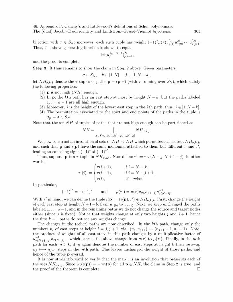
46. Appendix F: Cauchy’s and Littlewood’s definitions of Schur polynomials.The (dual) Jacobi–Trudi identity and Lindstrom–Gessel–Viennot bijections. 303

bijection with τ ∈ SN ; moreover, each such tuple has weight (−1)τµ(τ)uλ1τ(1)uλ2τ(2) · · ·u

λNτ(N).

Thus, the above generating function is shown to equal

det(uλk+N−kj )Nj,k=1,

and the proof is complete.

Step 3: It thus remains to show the claim in Step 2 above. Given parameters

σ ∈ SN , k ∈ [1, N ], j ∈ [1, N − k],

let NHσ,k,j denote the τ -tuples of paths p = (p, τ) (with τ running over SN ), which satisfythe following properties:

(1) p is not high (NH) enough.(2) In p, the kth path has an east step at most by height N − k, but the paths labeled

1, . . . , k − 1 are all high enough.(3) Moreover, j is the height of the lowest east step in the kth path; thus, j ∈ [1, N − k].(4) The permutation associated to the start and end points of the paths in the tuple is

σp = σ ∈ SN .

Note that the set NH of tuples of paths that are not high enough can be partitioned as

NH =⊔

σ∈SN , k∈[1,N ], j∈[1,N−k]

NHσ,k,j .

We now construct an involution of sets ι : NH → NH which permutes each subset NHσ,k,j ,and such that p and ι(p) have the same monomial attached to them but different τ and τ ′,

leading to canceling signs (−1)τ 6= (−1)τ′.

Thus, suppose p is a τ -tuple in NHσ,k,j . Now define τ ′ := τ (N − j,N + 1− j); in otherwords,

τ ′(i) :=

τ(i+ 1), if i = N − j;τ(i− 1), if i = N − j + 1;

τ(i), otherwise.

In particular,

(−1)τ′

= −(−1)τ and µ(τ ′) = µ(τ)uτ(N+1−j)u−1τ(N−j).

With τ ′ in hand, we can define the tuple ι(p) = (ι(p), τ ′) ∈ NHσ,k,j . First, change the weightof each east step at height N + 1− b, from uτ(b) to uτ ′(b). Next, we keep unchanged the pathslabeled 1, . . . , k−1, and in the remaining paths we do not change the source and target nodeseither (since σ is fixed). Notice that weights change at only two heights j and j + 1; hencethe first k − 1 paths do not see any weights change.

The changes in the (other) paths are now described. In the kth path, change only thenumbers nl of east steps at height l = j, j + 1, via: (nj , nj+1) 7→ (nj+1 + 1, nj − 1). Note,the product of weights of all east steps in this path changes by a multiplicative factor ofu−1τ(N+1−j)uτ(N−j) – which cancels the above change from µ(τ) to µ(τ ′). Finally, in the mth

path for each m > k, if nl again denotes the number of east steps at height l, then we swapnj ←→ nj+1 steps in the mth path. This leaves unchanged the weight of those paths, andhence of the tuple p overall.

It is now straightforward to verify that the map ι is an involution that preserves each ofthe sets NHσ,k,j . Since wt(ι(p)) = −wt(p) for all p ∈ NH, the claim in Step 2 is true, andthe proof of the theorem is complete.

304 Part 6: Bibliographic notes and references

Bibliographic notes and references

Most of the material in this part is taken from two papers: one by Belton–Guillot–Khare–Putinar [23] (see also [24] and [25] for summaries), and the other by Khare and Tao [217](see also its summary [216]). We list the remaining references. For preliminaries on Schurpolynomials, the standard reference is Macdonald’s monograph [246]. Theorem 44.6 on thecoordinatewise monotonicity of Schur polynomial ratios is proved using a deep result of Lam,Postnikov, and Pylyavskyy [231], following previous work by Skandera [338]. There are otherways to show this result, e.g., using Chebyshev blossoming as shown by Ait-Haddou in jointworks [6, 7], or by Dodgson condensation (see [217]). Theorem 44.8 is taken from [217] (thecoordinatewise non-decreasing property on (0,∞)N6= ). We also remark that Equation (42.11),

like Proposition 17.5, was recently extended to arbitrary polynomials and (formal) powerseries by the author in [214].

Theorem 45.2 and its proof are due to Hunter [187]. Appendix F follows Bressoud andWei [71], relying on the works of Karlin and McGregor [201, 202], Lindstrom [238], and Gesseland Viennot [142].

Bibliography 305

References

[1] Ivo Adan, Michael van Eenige, and Jacques Resing. Fitting discrete distributions on the first two mo-ments. Probab. Engrg. Inform. Sci., 9(4):623–632, 1995.

[2] Jim Agler and John Edward McCarthy. What can Hilbert spaces tell us about bounded functions inthe bidisk? In: A Glimpse at Hilbert Space Operators, Oper. Theory Adv. Appl., Vol. 207 (S. Axler,P. Rosenthal, D. Sarason, Eds.), pp. 81–97, 2010.

[3] Jim Agler, John Edward McCarthy, and Nicholas John Young. Operator Analysis: Hilbert space methodsin complex analysis. Cambridge Tracts in Mathematics 219, Cambridge University Press, Cambridge,2020.

[4] Michael Aissen, Albert Edrei, Isaac Jacob Schoenberg, and Anne M. Whitney. On the generating func-tions of totally positive sequences. Proc. Natl. Acad. Sci. USA, 37(5): 303–307, 1951.

[5] Michael Aissen, Isaac Jacob Schoenberg, and Anne M. Whitney. On the generating functions of totallypositive sequences I. J. d’Analyse Math., 2:93–103, 1952.

[6] Rachid Ait-Haddou and Marie-Laurence Mazure. The fundamental blossoming inequality in Chebyshevspaces–I: Applications to Schur functions. Found. Comput. Math., 18(1):135–158, 2018.

[7] Rachid Ait-Haddou, Yusuke Sakane, and Taishin Nomura. Chebyshev blossoming in Muntz spaces:Toward shaping with Young diagrams. J. Comput. Appl. Math., 247:172–208, 2013.

[8] Naum Ilyich Akhiezer. The classical moment problem and some related questions in analysis. Translatedby N. Kemmer. Hafner Publishing Co., New York, 1965.

[9] Arthur Albert. Conditions for positive and nonnegative definiteness in terms of pseudoinverses. SIAMJ. Appl. Math., 17(2), 434–440, 1969.

[10] Alexandru Aleman, Dmitry Beliaev, and Haakan Hedenmalm. Real zero polynomials and Polya–Schurtype theorems. J. d’Analyse Math., 94:49–60, 2004.

[11] Suprasad V. Amari and Ravindra Babu Misra. Closed-form expressions for distribution of sum of expo-nential random variables. IEEE Trans. Reliab., 46(4):519–522, 1997.

[12] Tsuyoshi Ando. Totally positive matrices. Linear Algebra Appl., 90:165–219, 1987.[13] Konstantin Alekseevich Andreev. Note sur une relation entre les integrales definies des produits des

fonctions. Mem. Soc. Sci. Phys. Nat. Bordeaux, 3(2):1–14, 1886.[14] Bernard A. Asner, Jr. On the total non-negativity of the Hurwitz matrix. SIAM J. Appl. Math.,

18(2):407–414, 1970.[15] Zhi Dong Bai and Li-Xin Zhang. Semicircle law for Hadamard products. SIAM J. Matrix Anal. Appl.,

29(2):473–495, 2007.[16] Mihaly Bakonyi and Hugo J. Woerdeman. Matrix completions, moments, and sums of Hermitian squares.

Princeton Series in Applied Mathematics, Princeton University Press, Princeton, 2011.[17] Stefan Banach. Sur l’equation fonctionelle f(x + y) = f(x) + f(y). Fund. Math., 1(1):123–124, 1920.[18] Ravindra B. Bapat and T.E.S. Raghavan. Nonnegative matrices and applications. Encyclopedia of Math-

ematics and its Applications, Vol. 64, Cambridge University Press, Cambridge, 1997.[19] Victor Simoes Barbosa and Valdir Antonio Menegatto. Strict positive definiteness on products of compact

two-point homogeneous spaces. Integral Trans. Spec. Funct., 28(1):56–73, 2017.[20] Alexander I. Barvinok. Low rank approximations of symmetric polynomials and asymptotic counting of

contingency tables. Preprint, arXiv:math.CO/0503170, 2005.[21] Richard Keith Beatson and Wolfgang zu Castell. Dimension hopping and families of strictly positive

definite zonal basis functions on spheres. J. Approx. Theory, 221:22–37, 2017.[22] Richard Keith Beatson, Wolfgang zu Castell, and Yuan Xu. A Polya criterion for (strict) positive-

definiteness on the sphere. IMA J. Numer. Anal., 34(2):550–568, 2014.[23] Alexander Belton, Dominique Guillot, Apoorva Khare, and Mihai Putinar. Matrix positivity preservers

in fixed dimension. I. Adv. Math., 298:325–368, 2016.[24] Alexander Belton, Dominique Guillot, Apoorva Khare, and Mihai Putinar. Matrix positivity preservers

in fixed dimension. Comptes Rendus Math., 354(2):143–148, 2016.[25] Alexander Belton, Dominique Guillot, Apoorva Khare, and Mihai Putinar. Schur polynomials and posi-

tivity preservers. Extended abstract, FPSAC 2016 Proceedings, Disc. Math. Theor. Comp. Sc., Vol. BC,pp. 155–166, 2016.

[26] Alexander Belton, Dominique Guillot, Apoorva Khare, and Mihai Putinar. Simultaneous kernels ofmatrix Hadamard powers. Linear Algebra Appl., 576:142–157, 2019.

[27] Alexander Belton, Dominique Guillot, Apoorva Khare, and Mihai Putinar. A panorama of positivity.Part I: Dimension free. In: Analysis of Operators on Function Spaces (The Serguei Shimorin Memorial

306 Bibliography

Volume; A. Aleman, H. Hedenmalm, D. Khavinson, M. Putinar, Eds.), pp. 117–165, Trends in Math.,Birkhauser, 2019. Parts 1 and 2 (unified) available at arXiv:math.CA/1812.05482.

[28] Alexander Belton, Dominique Guillot, Apoorva Khare, and Mihai Putinar. A panorama of positivity.Part II: Fixed dimension. In: Complex Analysis and Spectral Theory, Proceedings of the CRM Workshopheld at Laval University, QC, May 21–25, 2018 (G. Dales, D. Khavinson, J. Mashreghi, Eds.). CRMProceedings – AMS Contemporary Mathematics 743, pp. 109–150, American Mathematical Society,2020. Parts 1 and 2 (unified) available at arXiv:math.CA/1812.05482.

[29] Alexander Belton, Dominique Guillot, Apoorva Khare, and Mihai Putinar. Matrix compression alongisogenic blocks. Preprint, arXiv:math.RA/2010.14429, 2020.

[30] Alexander Belton, Dominique Guillot, Apoorva Khare, and Mihai Putinar. Hirschman–Widder densities.Preprint, arXiv:math.CA/2101.02129, 2021.

[31] Alexander Belton, Dominique Guillot, Apoorva Khare, and Mihai Putinar. Moment-sequence transforms.J. Eur. Math. Soc., in press; arXiv:math.CA/1610.05740.

[32] Alexander Belton, Dominique Guillot, Apoorva Khare, and Mihai Putinar. Totally positive kernels, Polyafrequency functions, and their transforms. J. d’Analyse Math., in press; arXiv:math.FA/2006.16213.

[33] Alexander Belton, Dominique Guillot, Apoorva Khare, and Mihai Putinar. Work in progress, 2021.

[34] Eduard W. Benz. Uber lineare, verschiebungstreue Funktionaloperatoren und die Nullstellen ganzerFunktionen. Comment. Helv. Math., 7:243–289, 1934.

[35] Arkady Berenstein, Sergey Fomin, and Andrei Zelevinsky. Parametrizations of canonical bases andtotally positive matrices. Adv. Math., 122:49–149, 1996.

[36] Arkady Berenstein and Andrei Zelevinsky. Total positivity in Schubert varieties. Comment. Math. Helv.,72(1):128–166, 1997.

[37] Arkady Berenstein and Andrei Zelevinsky. Tensor product multiplicities, canonical bases and totallypositive varieties. Invent. Math., 143:77–128, 2001.

[38] Felix Alexandrovich Berezin. Quantization in complex symmetric spaces. Izv. Akad. Nauk SSSR Ser.Mat., 39(2):363–402, 1975.

[39] Christian Berg, Jens Peter Reus Christensen, and Paul Ressel. Positive definite functions on abeliansemigroups. Math. Ann., 223(3):253–274, 1976.

[40] Christian Berg, Jens Peter Reus Christensen, and Paul Ressel. Harmonic Analysis on Semigroups:Theory of Positive Definite and Related Functions. Graduate Texts in Mathematics, Vol. 100, Springer,New York, 1984.

[41] Christian Berg, Ana Paula Peron, and Emilio Porcu. Schoenberg’s theorem for real and complex Hilbertspheres revisited. J. Approx. Theory, 228:58–78, 2018.

[42] Christian Berg and Emilio Porcu. From Schoenberg coefficients to Schoenberg functions. Constr. Approx.,45:217–241, 2017.

[43] Serge Bernstein. Recons sur les Proprietes Extremales et la Meilleure Approximation des FonctionsAnalytiques d’une Variable Reelle. Borel series of monographs, Gauthier-Villars, Paris, 1926.

[44] Serge Bernstein. Sur les fonctions absolument monotones. Acta Math., 52(1):1–66, 1929.[45] Rajendra Bhatia. Matrix analysis. Graduate Texts in Mathematics, Vol. 169, Springer, New York, 1997.[46] Rajendra Bhatia. Positive definite matrices. Princeton Series in Applied Mathematics, Princeton Uni-

versity Press, Princeton, 2015.[47] Rajendra Bhatia and Ludwig Elsner. Positivity preserving Hadamard matrix functions. Positivity,

11(4):583–588, 2007.[48] Peter John Bickel and Elizaveta Levina. Covariance regularization by thresholding. Ann. Statist.,

36(6):2577–2604, 2008.[49] Charles Biehler. Sur une classe d’equations algebriques dont toutes les racines sont reelles. J. reine

angew. Math., 87:350–352, 1879.[50] Garrett Birkhoff. Metric foundations of geometry. I. Trans. Amer. Math. Soc., 55:465–492, 1944.[51] Henry Blumberg. On convex functions. Trans. Amer. Math. Soc., 20:40–44, 1919.[52] Leonard Mascot Blumenthal. New theorems and methods in determinant theory. Duke Math. J.,

2(2):396–404, 1936.[53] Ralph Philip Boas, Jr. The Stieltjes moment problem for functions of bounded variation. Bull. Amer.

Math. Soc., 45:399–404, 1939.[54] Ralph Philip Boas, Jr. Functions with positive derivatives. Duke Math. J., 8(1):163–172, 1941.[55] Ralph Philip Boas, Jr. and David Vernon Widder. Functions with positive differences. Duke Math. J.,

7:496–503, 1940.

Bibliography 307

[56] Salomon Bochner. Monotone funktionen, Stieltjessche integrale und harmonische analyse. Math. Ann.,108(1):378–410, 1933.

[57] Salomon Bochner. Hilbert distances and positive definite functions. Ann. of Math. (2), 42:647–656, 1941.[58] Rafaela Neves Bonfim, Jean Carlo Guella, and Valdir Antonio Menegatto. Strictly positive definite

functions on compact two-point homogeneous spaces: the product alternative. Symm., Integr. Geom.:Meth. Appl. (SIGMA), 14:112, 14 pp., 2018.

[59] Carl de Boor. On calculating with B-splines. J. Approx. Theory, 6(1):50–62, 1972.[60] Julius Borcea and Petter Branden. Applications of stable polynomials to mixed determinants: Johnson’s

conjectures, unimodality, and symmetrized Fischer products. Duke Math. J., 143(2):205–223, 2008.[61] Julius Borcea and Petter Branden. Polya–Schur master theorems for circular domains and their bound-

aries. Ann. of Math. (2), 170(1):465–492, 2009.[62] Julius Borcea and Petter Branden. The Lee–Yang and Polya–Schur programs. I. Linear operators pre-

serving stability. Invent. Math., 177(3):541–569, 2009.[63] Julius Borcea and Petter Branden. The Lee–Yang and Polya–Schur programs. II. Theory of stable

polynomials and applications. Comm. Pure Appl. Math., 62(12):1595–1631, 2009.[64] Julius Borcea and Petter Branden. Multivariate Polya–Schur classification problems in the Weyl algebra.

Proc. London Math. Soc., 101(1):73–104, 2016.[65] Julius Borcea, Petter Branden, and Thomas M. Liggett. Negative dependence and the geometry of

polynomials. J. Amer. Math. Soc., 22(2):521–567, 2009.[66] James Borger. Witt vectors, semirings, and total positivity. In: Absolute Arithmetic and F1-Geometry

(K. Thas, Ed.), pp. 273–331, Eur. Math. Soc., 2016.[67] James Borger and Darij Grinberg. Boolean Witt vectors and an integral Edrei–Thoma theorem. Selecta

Math. (NS), 22:595–629, 2016.[68] Petter Branden. On linear transformations preserving the Polya frequency property. Trans. Amer. Math.

Soc., 358(8):3697–3716, 2006.[69] Francesco Brenti. Unimodal, log-concave, and Polya frequency sequences in combinatorics. Mem. Amer.

Math. Soc., Vol. 413, American Mathematical Society, Providence, 1989.[70] Francesco Brenti. Combinatorics and total positivity. J. Combin. Theory Ser. A, 71(2):175–218, 1995.[71] David Marius Bressoud and Shi-Yuan Wei. Combinatorial equivalence of definitions of the Schur function.

AMS Contemp. Math., 143:59–64 (A Tribute to Emil Grosswald: Number Theory and Related Analysis),1993.

[72] Lawrence D. Brown, Iain M. Johnstone, and K. Brenda Macgibbon. Variation diminishing convolutionkernels associated with second-order differential operators. J. Amer. Statist. Assoc., 76(376):824–832,1981.

[73] Nicolaas Govert de Bruijn. Some theorems on the roots of polynomials. Nieuw Arch. Wiskunde, 23:66–68,1949.

[74] Victor Matveevich Buchstaber and Aleksei Antonovich Glutsyuk. Total positivity, Grassmannian andmodified Bessel functions. AMS Contemp. Math., 733:97–108 (Functional Analysis and Geometry: SelimGrigorievich Krein Centennial), 2019.

[75] Francois Budan de Boislaurent. Nouvelle methode pour la resolution des equations numeriques. Courcier,Paris, 1807.

[76] David A. Cardon, Tamas Forgacs, Andrzej Piotrowski, Evan Sorensen, and Jason C. White. On zero-sector reducing operations. J. Math. Anal. Appl., 468(1):480–490, 2018.

[77] Augustin-Louis Cauchy. Memoire sur les integrales definies, prises entre des limites imaginaires. DeBure freres, Paris, 1825.

[78] Arthur Cayley. On a theorem in the geometry of position. Cambridge Math. J., II:267–271, 1841.[79] Debao Chen, Valdir Antonio Menegatto, and Xingping Sun. A necessary and sufficient condition for

strictly positive definite functions on spheres. Proc. Amer. Math. Soc., 131(9):2733–2740, 2003.[80] Projesh Nath Choudhury. Characterizing total positivity: single vector tests via Linear Complementarity,

sign non-reversal, and variation diminution. Preprint, arXiv:math.RA/2103.05624, 2021.[81] Projesh Nath Choudhury, M. Rajesh Kannan, and Apoorva Khare. Sign non-reversal property for totally

non-negative and totally positive matrices and testing total positivity of their interval hull. Bull. LondonMath. Soc., 53(4):981–990, 2021.

[82] Jens Peter Reus Christensen and Paul Ressel. Functions operating on positive definite matrices and atheorem of Schoenberg. Trans. Amer. Math. Soc., 243:89–95, 1978.

308 Bibliography

[83] Jens Peter Reus Christensen and Paul Ressel. Positive definite kernels on the complex Hilbert sphere.Math. Z., 180(2):193–201, 1982.

[84] Henry Cohn and Matthew de Courcy-Ireland. The Gaussian core model in high dimensions. Duke Math.J., 167(13):2417–2455, 2018.

[85] Henry Cohn and Abhinav Kumar. Universally optimal distribution of points on spheres. J. Amer. Math.Soc., 20(1):99–148, 2007.

[86] Henry Cohn and Jeechul Woo. Three-point bounds for energy minimization. J. Amer. Math. Soc.,25(4):929–958, 2012.

[87] Henry Cohn and Yufei Zhao. Sphere packing bounds via spherical codes. Duke Math. J., 163(10):1965–2002, 2014.

[88] John Bligh Conway. Functions of one complex variable. Graduate Texts in Mathematics, Vol. 11,Springer, New York, 1978.

[89] Vincent Frederick Cowling and Wolfgang Joseph Thron. Zero-free regions of polynomials. Amer. Math.Monthly, 61(10):682–687, 1954.

[90] Trevor F. Cox and Michael A.A. Cox. Multidimensional scaling. In: Handbook of Data Visualization(C.-h. Chen, W. Hardle, and A. Unwin, Eds.), pp. 315–347, Springer, Berlin–Heidelberg, 2008.

[91] Thomas Craven and George Csordas. Composition theorems, multiplier Sequences and complex zerodecreasing sequences. In: Value distribution theory and related topics (G. Barsegian, I. Laine, C.C. Yang(Eds.), pp. 131–166, Advances in Complex Analysis and Its Applications, Vol. 3, Springer, Boston, 2014.

[92] Thomas Craven, George Csordas, and Wayne Smith. The zeros of derivatives of entire functions and thePolya–Wiman Conjecture. Ann. of Math. (2), 125(2):405–431, 1987.

[93] Colin Walker Cryer. The LU-factorization of totally positive matrices. Linear Algebra Appl., 7(1):83–92,1973.

[94] Colin Walker Cryer. Some properties of totally positive matrices. Linear Algebra Appl., 15(1):1–25, 1976.[95] Haskell Brooks Curry and Isaac Jacob Schoenberg. On spline distributions and their limits: The Polya

distribution functions. Bull. Amer. Math. Soc., 53(11):1114, 1947.[96] Haskell Brooks Curry and Isaac Jacob Schoenberg. On Polya frequency functions IV: The fundamental

spline functions and their limits. J. d’Analyse Math., 17:71–107, 1966.[97] David Raymond Curtiss. Recent extensions of Descartes’ Rule of Signs. Ann. of Math. (2), 19(4):251–278,

1918.[98] Yuri L’vovich Dalestkii and Selim Grigorievich Krein. Integration and differentiation of functions of

Hermitian operators and applications to the theory of perturbations (Russian). Voronoez. Gos. Univ.Trudy Sem. Funkcional. Anal., vol. 1, pp. 81–105 (1956); AMS Translations: Ser. 2, vol. 47, pp. 1–30,1965.

[99] Aleksey Aleksandrovich Davydov. Totally positive sequences and R-matrix quadratic algebras. J. Math.Sci., 100(1):1871–1876, 2000.

[100] Rene Descartes. Le Geometrie. Appendix to Discours de la methode, 1637.[101] Dimitar Kolev Dimitrov and Juan Manuel Pena. Almost strict total positivity and a class of Hurwitz

polynomials. Linear Algebra Appl., 132(2):212–223, 2005.[102] Dimitar Kolev Dimitrov and Yuan Xu. Wronskians of Fourier and Laplace transforms. Trans. Amer.

Math. Soc., 372(6):4107–4125, 2019.[103] William Francis Donoghue Jr. Monotone matrix functions and analytic continuation. Grundlehren der

mathematischen Wissenschaften, Vol. 207, Springer-Verlag, Berlin, 1974.[104] Alexander Dyachenko. Total nonnegativity of infinite Hurwitz matrices of entire and meromorphic func-

tions. Complex Anal. Oper. Theory, 8:1097–1127, 2014.[105] Harry Dym and Victor Emmanuilovich Katsnelson. Contributions of Issai Schur to analysis. In: Studies

in Memory of Issai Schur (A. Joseph, A. Melnikov, and R. Rentschler, Eds.), pp. xci–clxxxiii, Progressin Math., Vol. 210, Birkhauser, Basel, 2003.

[106] Albert Edrei. On the generating functions of totally positive sequences II. J. d’Analyse Math., 2:104–109,1952.

[107] Albert Edrei. Proof of a conjecture of Schoenberg on the generating function of a totally positive se-quence. Canad. J. Math., 5:86–94, 1953.

[108] Albert Edrei. On the generation function of a doubly infinite, totally positive sequence. Trans. Amer.Math. Soc., 74:367–383, 1953.

[109] Bradley Efron. Increasing properties of Polya frequency functions. Ann. Math. Statist., 36(1):272–279,1965.

Bibliography 309

[110] Noureddine El Karoui. Operator norm consistent estimation of large-dimensional sparse covariance ma-trices. Ann. Statist., 36(6):2717–2756, 2008.

[111] Jan Emonds and Hartmut Fuhr. Strictly positive definite functions on compact abelian groups. Proc.Amer. Math. Soc., 139(3):1105–1113, 2011.

[112] Shaun Michael Fallat and Charles Royal Johnson. Totally nonnegative matrices. Princeton Series inApplied Mathematics, Princeton University Press, Princeton, 2011.

[113] Shaun Michael Fallat, Charles Royal Johnson, and Alan David Sokal. Total positivity of sums, Hadamardproducts and Hadamard powers: Results and counterexamples. Linear Algebra Appl., 520:242–259, 2017;Corrigendum, Linear Algebra Appl., 613:393–396, 2021.

[114] Ky Fan. Some matrix inequalities. Abh. Math. Sem. Univ. Hamburg, 29:185–196, 1966.[115] Jacques Faraut. Formule du binome generalisee. In: Harmonic Analysis, Lecture Notes in Math.,

Vol. 1359, pp. 170–180, Springer, Berlin, 1988.

[116] Jacques Faraut and Adam Koranyi. Function spaces and reproducing kernels on bounded symmetricdomains. J. Funct. Anal., 88(1):64–89, 1990.

[117] Jacques Faraut and Adam Koranyi. Analysis on symmetric cones. Oxford Mathematical Monographs.The Clarendon Press, Oxford University Press, New York, second edition, 1994. Oxford Science Publi-cations.

[118] Mihaly Fekete and Georg Polya. Uber ein Problem von Laguerre. Rend. Circ. Mat. Palermo, 34:89–120,1912.

[119] William Feller. An introduction to probability theory and its applications (1st ed.). Wiley & Sons, NewYork, xviii+636 pp., 1966.

[120] Miroslav Fiedler and Thomas Markham. An observation on the Hadamard product of Hermitian matri-ces. Linear Algebra Appl., 215:179–182, 1995.

[121] Miroslav Fiedler and Vlastimil Ptak. On matrices with non-positive off-diagonal elements and positiveprincipal minors. Czech. Math. J., 12(3):382–400, 1962.

[122] Steve Fisk. Polynomials, roots, and interlacing. Version 2, arXiv:math.CA/0612833, 2008.[123] Carl Hanson FitzGerald and Roger Alan Horn. On fractional Hadamard powers of positive definite

matrices. J. Math. Anal. Appl., 61(3):633–642, 1977.[124] Carl Hanson FitzGerald, Charles Anthony Micchelli, and Allan Pinkus. Functions that preserve families

of positive semidefinite matrices. Linear Algebra Appl., 221:83–102, 1995.[125] Sergey Fomin and Andrei Zelevinsky. Double Bruhat cells and total positivity. J. Amer. Math. Soc.,

12(2):335–380, 1999.[126] Sergey Fomin and Andrei Zelevinsky. Total positivity: Tests and parametrizations. Math. Intelligencer,

22(1):23–33, 2000.[127] Sergey Fomin and Andrei Zelevinsky. Cluster algebras. I. Foundations. J. Amer. Math. Soc., 15(2):497–

529, 2002.[128] Yanik-Pascal Forster, Mario Kieburg, and Holger Kosters. Polynomial ensembles and Polya frequency

functions. J. Theor. Probab., in press; arXiv:math.PR/1710.08794.[129] Jean-Baptiste Joseph Fourier. Sur l’usage du theoreme de Descartes dans la recherche des limites des

racines. Bull. Sci. Soc. Phil. Paris, 156–165 and 181–187, Gauthier–Villars, Paris, 1820.[130] Maurice Rene Frechet. Les dimensions d’un ensemble abstrait. Math. Ann., 68:145–168, 1910.[131] Maurice Rene Frechet. Sur la definition axiomatique d’une classe d’espaces vectoriels distancies appli-

cables vectoriellement sur l’espace de Hilbert. Ann. of Math. (2), 36(3):705–718, 1935.[132] Kurt Otto Friedrichs. The identity of weak and strong extensions of differential operators. Trans. Amer.

Math. Soc., 55:132–151, 1944.[133] Matsusaboro Fujiwara. Einige Bemerkungen uber die elementare Theorie der algebraischen Gleichungen.

Tohoku Math. J., 9:102–108, 1916.[134] David Gale and Hukukane Nikaido. The Jacobian matrix and global univalence of mappings. Math.

Ann., 159:81–93, 1965.[135] Feliks Ruvimovich Gantmacher. Sur les noyaux de Kellogg non symmetriques. Comptes Rendus (Dok-

lady) Acad. Sci. de l’URSS, 1(10):3–5, 1936.[136] Feliks Ruvimovich Gantmacher. The theory of matrices. Vols. 1, 2. Translated by K.A. Hirsch. Chelsea

Publishing Co., New York, 1959.[137] Feliks Ruvimovich Gantmacher and Mark Grigor’evich Krein. Sur les matrices completement non

negatives et oscillatoires. Compositio Math., 4:445–476, 1937.

310 Bibliography

[138] Feliks Ruvimovich Gantmacher and Mark Grigor’evich Krein. Oscillation matrices and kernels and smallvibrations of mechanical systems. Translated by A. Eremenko. Chelsea Publishing Co., New York, 2002.

[139] Jurgen Garloff. Intervals of almost totally positive matrices. Linear Algebra Appl., 363:103–108, 2003.[140] Jurgen Garloff and David G. Wagner. Hadamard products of stable polynomials are stable. J. Math.

Anal. Appl., 202(3):797–809, 1996.[141] Total positivity and its applications (M. Gasca and C.A. Micchelli, Eds.). Proceedings of Jaca Meeting

(1994), Mathematics and its Applications, Vol. 359, Kluwer, Dordrecht, 1996.[142] Ira Gessel and Xavier Viennot. Binomial determinants, paths, and hook length formulae. Adv. Math.,

58(3):300–321, 1985.[143] Simon Grigorevich Gindikin. Invariant generalized functions in homogeneous domains. Funct. Anal.

Appl., 9:50–52, 1975.[144] Tillmann Gneiting. Strictly and non-strictly positive definite functions on spheres. Bernoulli, 19(4):1327–

1349, 2013.

[145] Piotr Graczyk, Jacek Malecki, and Eberhard Mayerhofer. A characterization of Wishart processes andWishart distributions. Stoch. Proc. Appl., 128(4):1386–1404, 2018.

[146] Kenneth Ralph Goodearl, Stephane Launois, and Tom H. Lenagan. Totally nonnegative cells and matrixPoisson varieties. Adv. in Math., 226(1):779–826, 2011.

[147] Karlheinz Grochenig. Schoenberg’s theory of totally positive functions and the Riemann zeta function.Preprint, arXiv:math.NT/2007.12889, 2020.

[148] Karlheinz Grochenig, Jose Luis Romero, and Joachim Stockler. Sampling theorems for shift-invariantspaces, Gabor frames, and totally positive functions. Invent. Math., 211:1119–1148, 2018.

[149] Karlheinz Grochenig and Joachim Stockler. Gabor frames and totally positive functions. Duke Math. J.,162(6):1003–1031, 2013.

[150] Jean Carlo Guella, Valdir Antonio Menegatto, and Ana Paula Peron. Strictly positive definite kernelson a product of circles. Positivity, 21:329–342, 2017.

[151] Dominique Guillot, Apoorva Khare, and Bala Rajaratnam. Complete characterization of Hadamardpowers preserving Loewner positivity, monotonicity, and convexity. J. Math. Anal. Appl., 425(1):489–507, 2015.

[152] Dominique Guillot, Apoorva Khare, and Bala Rajaratnam. Preserving positivity for matrices with spar-sity constraints. Trans. Amer. Math. Soc., 368(12):8929–8953, 2016.

[153] Dominique Guillot, Apoorva Khare, and Bala Rajaratnam. Critical exponents of graphs. J. Combin.Theory Ser. A, 139:30–58, 2016.

[154] Dominique Guillot, Apoorva Khare, and Bala Rajaratnam. The critical exponent: a novel graph invari-ant. Sem. Lothar. Combin., 78B, article 62, 12 pp., 2017.

[155] Dominique Guillot, Apoorva Khare, and Bala Rajaratnam. Preserving positivity for rank-constrainedmatrices. Trans. Amer. Math. Soc., 369(9):6105–6145, 2017.

[156] Dominique Guillot and Bala Rajaratnam. Retaining positive definiteness in thresholded matrices. LinearAlgebra Appl., 436(11):4143–4160, 2012.

[157] Dominique Guillot and Bala Rajaratnam. Functions preserving positive definiteness for sparse matrices.Trans. Amer. Math. Soc., 367(1):627–649, 2015.

[158] Jacques Salomon Hadamard. Essai sur l’etude des fonctions donnees par leur developpement de Taylor.J. Math. Pures Appl., 8:101–186, 1892.

[159] Jacques Salomon Hadamard. Etude sur les proprites des fonctions entieres et an particulier d’une fonctionconsideree par Riemann. J. Math. Pures Appl., 171–215, 1893.

[160] Jacques Salomon Hadamard. Theoreme sur les series entieres. Acta Math., 22:55–63, 1899.[161] Hans Ludwig Hamburger. Bemerkungen zu einer Fragestellung des Herrn Polya. Math. Z., 7:302–322,

1920.[162] Hans Ludwig Hamburger. Uber eine Erweiterung des Stieltjesschen Momentenproblems. Math. Ann.,

Part I, Vol. 81, pp. 235–319, 1920; Part II, Vol. 82, pp. 120–164, 1921; Part III, Vol. 82, pp. 168–187,1921.

[163] Berthold Heiligers. Totally nonnegative moment matrices. Linear Algebra Appl., 199 (suppl. 1):213–227,1994.

[164] Henry Helson, Jean-Pierre Kahane, Yitzhak Katznelson, and Walter Rudin. The functions which operateon Fourier transforms. Acta Math., 102(1):135–157, 1959.

Bibliography 311

[165] Charles Hermite. Extrait d’une lettre de Mr. Ch. Hermite de Paris a Mr. Borchardt de Berlin sur lenombre des racines d’une equation algebrique comprises entre des limites donnees. J. reine angew. Math.,52:39–51, 1856.

[166] Charles Hermite. Questions 777, 778, 779. Nouv. Ann. Math., 5:pp. 432, 479, 1866.[167] Alfred Hero and Bala Rajaratnam. Large-scale correlation screening. J. Amer. Statist. Assoc.,

106(496):1540–1552, 2011.[168] Alfred Hero and Bala Rajaratnam. Hub discovery in partial correlation graphs. IEEE Trans. Inform.

Theory, 58(9):6064–6078, 2012.[169] Daniel Hershkowitz, Michael Neumann, and Hans Schneider. Hermitian positive semidefinite matrices

whose entries are 0 or 1 in modulus. Linear Multilinear Algebra, 46(4):259–264, 1999.[170] Carl S. Herz. Fonctions operant sur les fonctions definies-positives. Ann. Inst. Fourier (Grenoble),

13:161–180, 1963.[171] Fumio Hiai. Monotonicity for entrywise functions of matrices. Linear Algebra Appl., 431(8):1125–1146,

2009.[172] Fumio Hiai and Denes Petz. Introduction to matrix analysis and applications. Universitext, Springer,

Cham, 2014, viii+332 pp.[173] David Hilbert. Uber die Darstellung definiter Formen als Summe von Formenquadraten. Math. Ann.,

32:342–350, 1888.[174] David Hilbert. Uber ternare definite Formen. Acta Math., 17:169–197, 1893.[175] Isidore Isaac Hirschman Jr. and David Vernon Widder. The inversion of a general class of convolution

transforms. Trans. Amer. Math. Soc., 66(1):135–201, 1949.[176] Isidore Isaac Hirschman Jr. and David Vernon Widder. The convolution transform. Princeton Legacy

Library, Princeton University Press, Princeton, 1955.[177] Phung Ho Hai. Poincare series of quantum spaces associated to Hecke operators. Acta Math. Vietnam.,

24(2):235–246, 1999.[178] Thomas Hofmann, Bernhard Scholkopf, and Alexander J. Smola. Kernel methods in machine learning.

Ann. Statist., 36(3):1171–1220, 2008.[179] Olga Holtz. Hermite–Biehler, Routh–Hurwitz, and total positivity. Linear Algebra Appl., 372:105–110,

2003.[180] Olga Holtz, Sergey Khrushchev, and Olga Kushel. Generalized Hurwitz matrices, generalized Euclidean

algorithm, and forbidden sectors of the complex plane. Comput. Methods Funct. Theory, 16:395–431,2016.

[181] Olga Holtz and Mikhail Tyaglov. Structured matrices, continued fractions, and root localization ofpolynomials. SIAM Rev., 54(3):421–509, 2012.

[182] Roger Alan Horn. The theory of infinitely divisible matrices and kernels. Trans. Amer. Math. Soc.,136:269–286, 1969.

[183] Roger Alan Horn and Charles Royal Johnson. Matrix analysis. Cambridge University Press, Cambridge,1985.

[184] Roger Alan Horn and Charles Royal Johnson. Topics in matrix analysis. Cambridge University Press,Cambridge, 1991.

[185] Loo-Keng Hua. Harmonic analysis of functions of several complex variables in the classical domains.Translations of Mathematical Monographs, Vol. 6, American Mathematical Society, Providence, 1963.

[186] Hsin-Yuan Huang and Chih-Jen Lin. Linear and kernel classification: When to use which? Proc. 2016SIAM Conf. Data Min., 216–224, 2016.

[187] David Boss Hunter. The positive-definiteness of the complete symmetric functions of even order. Math.Proc. Camb. Phil. Soc., 82(2):255–258, 1977.

[188] Adolf Hurwitz. Uber die Bedingungen, unter welchen eine Gleichung nur Wurzeln mit negativen reellenTheilen besitzt. Math. Ann., 46:273–284, 1895.

[189] Adolf Hurwitz. Uber den Satz von Budan–Fourier. Math. Ann., 71:584–591, 1911.[190] Carl Gustav Jacob Jacobi. De formatione et proprietatibus Determinatium. J. reine angew. Math.,

22:285–318, 1841.[191] Tanvi Jain. Hadamard powers of some positive matrices. Linear Algebra Appl., 528:147–158, 2017.[192] Tanvi Jain. Hadamard powers of rank two, doubly nonnegative matrices. Adv. in Oper. Theory, 5:839–

849, 2020 (Rajendra Bhatia volume).[193] Graham James Oscar Jameson. Counting zeros of generalised polynomials: Descartes’ rule of signs and

Laguerre’s extensions. The Mathematical Gazette, 90(518):223–234, 2006.

312 Bibliography

[194] Johan Ludwig William Valdemar Jensen. Recherches sur la theorie des equations. Acta. Math., 36:181–195, 1913.

[195] Robert Jentzsch. Uber Integralgleichungen mit positivem Kern. J. reine angew. Math., 141:235–244,1912.

[196] Charles Royal Johnson and Ronald L. Smith. Line insertions in totally positive matrices. J. Approx.Theory, 105:305–312, 2000.

[197] Charles Royal Johnson and Olivia Walch. Critical exponents: Old and new. Electr. J. Linear Alg.,25:72–83, 2012.

[198] Richard V. Kadison and Isadore Manuel Singer. Extensions of pure states. Amer. J. Math., 81(2):383–400, 1959.

[199] Samuel Karlin. Total positivity, absorption probabilities and applications. Trans. Amer. Math. Soc.,111:33–107, 1964.

[200] Samuel Karlin. Total positivity. Vol. 1. Stanford University Press, Stanford, 1968.[201] Samuel Karlin and James McGregor. Coincidence probabilities of birth and death processes. Pacific J.

Math., 9(4):1109–1140, 1959.[202] Samuel Karlin and James McGregor. Coincidence probabilities. Pacific J. Math., 9(4):1141–1164, 1959.[203] Samuel Karlin, Frank Proschan, and Richard Eugene Barlow. Moment inequalities of Polya frequency

functions. Pacific J. Math., 11(3):1023–1033, 1961.[204] Samuel Karlin and Yosef Rinott. Classes of orderings of measures and related correlation inequalities. I.

Multivariate totally positive distributions. J. Multivariate Anal., 10(4):467–498, 1980.[205] Samuel Karlin and Yosef Rinott. Total positivity properties of absolute value multinormal variables

with applications to confidence interval estimates and related probabilistic inequalities. Ann. Statist.,9(5):1035–1049, 1981.

[206] Samuel Karlin and Zvi Ziegler. Chebyshevian spline functions. SIAM J. Numer. Anal., 3(3):514–543,1966.

[207] Olga M. Katkova. A certain method for constructing Polya frequency sequences. J. Soviet Math.,52:3539–3545, 1990.

[208] Olga M. Katkova. Multiple positivity and the Riemann zeta-function. Comput. Methods Funct. Theory,7:13–31, 2007.

[209] Olga M. Katkova and Anna M. Vishnyakova. On sufficient conditions for the total positivity and for themultiple positivity of matrices. Linear Algebra Appl., 16(2–3):1083–1097, 2006.

[210] Olga M. Katkova and Anna M. Vishnyakova. A sufficient condition for a polynomial to be stable. J.Math. Anal. Appl., 347(1):81–89, 2008.

[211] Oliver Dimon Kellogg. Orthogonal function sets arising from integral equations. Amer. J. Math.,40(2):145–154, 1918.

[212] Johannes Henricus Bernardus Kemperman. A Hurwitz matrix is totally positive. SIAM J. Math. Anal.,13(2):331–341, 1982.

[213] Apoorva Khare. Sharp nonzero lower bounds for the Schur product theorem. Proc. Amer. Math. Soc.,149(12):5049–5063, 2021.

[214] Apoorva Khare. Smooth entrywise positivity preservers, a Horn–Loewner master theorem, and symmet-ric function identities. Trans. Amer. Math. Soc., in press; arXiv:math.CA/1809.01823.

[215] Apoorva Khare. Critical exponents for total positivity, individual kernel encoders, and the Jain–Karlin–Schoenberg kernel. Preprint, arXiv:math.FA/2008.05121, 2020.

[216] Apoorva Khare and Terence Tao. Schur polynomials, entrywise positivity preservers, and weak majoriza-tion. Sem. Lothar. Combin., 80B, article 14, 12 pp., 2018.

[217] Apoorva Khare and Terence Tao. On the sign patterns of entrywise positivity preservers in fixed dimen-sion. Amer. J. Math., 143(6):1863–1929, 2021.

[218] Jee Soo Kim and Frank Proschan. Total positivity. In: Encyclopedia of Statistical Sciences (S. Kotz etal, Eds.), Vol. 14, Wiley, New York, pp. 8665–8672, 2006.

[219] Jiae Kim, Yoonkyung Lee, and Zhiyu Liang. The geometry of nonlinear embeddings in kernel discrimi-nant analysis. Preprint, http://arxiv.org/abs/2005.05546, 2020.

[220] Tinne Hoff Kjeldsen. The early history of the moment problem. Historia Math., 20(1):19–44, 1993.[221] Yuji Kodama and Lauren Williams. KP solitons, total positivity and cluster algebras. Proc. Natl. Acad.

Sci. USA, 108:8984–8989, 2011.[222] Yuji Kodama and Lauren Williams. KP solitons and total positivity for the Grassmannian. Invent.

Math., 198(3):637–699, 2014.

Bibliography 313

[223] Andrey Nikolaevich Kolmogorov. Kurven in Hilbertschen Raum, die gegenuber einer einparametrigenGruppe von Bewegungen invariant sind. C.R. Doklady Acad. Sci. U.R.S.S. 26:6–9, 1940.

[224] Jacob Korevaar. The zeros of approximating polynomials and the canonical representation of an entirefunction. Duke Math. J., 18(2):573–592, 1951.

[225] Jacob Korevaar. Entire functions as limits of polynomials. Duke Math. J., 21(2):533–548, 1954.[226] Bertram Kostant and Siddhartha Sahi. The Capelli identity, tube domains, and the generalized Laplace

transform. Adv. Math., 87(1):71–92, 1991.[227] Steven George Krantz and Harold Raymond Parks. A primer of real analytic functions. Birkhauser

Advanced Texts, Birkhauser, Boston, xiii+209 pp., 2002.[228] Edmond Laguerre. Sur les fonctions du genre zero et du genre un. C. R. Acad. Sci. Paris, 95:828–831,

1882.[229] Edmond Laguerre. Memoire sur la theorie des equations numeriques. J. Math. Pures Appl., 9:9–146,

1883.[230] Edmond Laguerre. Sur quelques points de la theorie des equations numeriques. Acta Math., 4:97–120,

1884.[231] Thomas Lam, Alexander E. Postnikov, and Pavlo Pylyavskyy. Schur positivity and Schur log-concavity.

Amer. J. Math., 129(6):1611–1622, 2007.[232] Michel Lassalle. Algebre de Jordan et ensemble de Wallach. Invent. Math., 89(2):375–393, 1987.[233] Tsung-Dao Lee and Chen Ning Yang. Statistical theory of equations of state and phase transitions. II.

Lattice gas and Ising model. Phys. Rev., 87:410–419, 1952.[234] Gerard Letac and Helene Massam. The Laplace transform (det s)−p exp tr(s−1w) and the existence of

non-central Wishart distributions. J. Multivar. Anal., 163:96–110, 2018.[235] Boris Yakovlevich Levin. Distribution of zeros of entire functions. Translations of Mathematical Mono-

graphs, Vol. 5, Translated from the Russian by R.P. Boas Jr., J.M. Danskin, F.M. Goodspeed, J. Kore-vaar, A.L. Shields, and H.P. Thielman, American Mathematical Society, Providence, 1980.

[236] Ai Li and Steve Horvath. Network neighborhood analysis with the multi-node topological overlap mea-sure. Bioinformatics, 23(2):222–231, 2007.

[237] Leo Liberti and Carlile Lavor. Six mathematical gems from the history of distance geometry. Int. Trans.Oper. Res., 23(5):897–920, 2016.

[238] Bernt Lindstrom. On the vector representations of induced matroids. Bull. London Math. Soc., 5(1):85–90, 1973.

[239] Egon Lindwart and Georg Polya. Uber einen zusammenhang zwischen der konvergenz von polynomfolgenund der verteilung ihrer wurzeln. Rend. Circ. Mat. Palermo, 37:279–304, 1914.

[240] Charles Loewner. Uber monotone Matrixfunktionen. Math. Z., 38(1):177–216, 1934.[241] Charles Loewner. On totally positive matrices. Math. Z., 63:338–340, 1955 (Issai Schur memorial vol-

ume).[242] Charles Loewner. Determination of the critical exponent of the Green’s function. 1965 Symposium on

Function Theory, Erevan, USSR, 1966.[243] Charles Loewner. On schlicht-monotonic functions of higher order. J. Math. Anal. Appl., 14(2):320–325,

1966.[244] Felix Lucas. Proprietes geometriques des fractionnes rationnelles. C. R. Acad. Sci. Paris, 77:431–433,

1874.[245] George Lusztig. Total positivity in reductive groups, Lie theory and geometry. Progr. Math., Vol. 123,

Birkhauser Boston, Boston, MA, 1994, pp. 531–568.George Lusztig. Total positivity and canonical bases. In: Algebraic groups and Lie groups (G.I. Lehrer,Ed.), Austral. Math. Soc. Lect. Ser., Vol. 9, Cambridge University Press, Cambridge, 1997, pp. 281–295.

[246] Ian Grant Macdonald. Symmetric functions and Hall polynomials. Oxford Mathematical Monographs.The Clarendon Press, Oxford University Press, New York, second edition, 1995. With contributions byA. Zelevinsky, Oxford Science Publications.

[247] Nathaniel Macon and Abraham Spitzbart. Inverses of Vandermonde matrices. Amer. Math. Monthly,65(2):95–100, 1958.

[248] Ernest Malo. Note sur les equations algebriques dont toutes les racines sont reelles. J. Math. Spec.(Ser. 4), 4:7–10, 1895.

[249] Adam W. Marcus, Daniel A. Spielman, and Nikhil Srivastava. Interlacing families I: Bipartite Ramanujangraphs of all degrees. Ann. of Math. (2), 182(1):307–325, 2015.

314 Bibliography

[250] Adam W. Marcus, Daniel A. Spielman, and Nikhil Srivastava. Interlacing families II. Mixed characteristicpolynomials and the Kadison-Singer problem. Ann. of Math. (2), 182(1):327–350, 2015.

[251] Adam W. Marcus, Daniel A. Spielman, and Nikhil Srivastava. Interlacing families IV. Bipartite Ra-manujan graphs of all sizes. SIAM J. Comput., 47(6):2488–2509, 2018.

[252] Marvin David Marcus and Nisar A. Khan. A note on the Hadamard product. Canad. Math. Bull.,2(2):81–83, 1959.

[253] Michael Margaliot and Eduardo D. Sontag. Revisiting totally positive differential systems: A tutorialand new results. Automatica, 101:1–14, 2019.

[254] Eberhard Mayerhofer. On Wishart and noncentral Wishart distributions on symmetric cones. Trans.Amer. Math. Soc., 371(10):7093–7109, 2019.

[255] Valdir Antonio Menegatto and Claudemir Pinheiro Oliveira. Positive definiteness on products of compacttwo-point homogeneous spaces and locally compact abelian groups. Canad. Math. Bull., 63(4):705–715,2020.

[256] Valdir Antonio Menegatto and Ana Paula Peron. Positive definite kernels on complex spheres. J. Math.Anal. Appl., 254(1):219–232, 2001.

[257] Karl Menger. Die Metrik des Hilbertschen Raumes. Anz. Akad. Wissen. Wien, Math. Nat. Kl., 65:159–160, 1928.

[258] Karl Menger. Untersuchungen uber allgemeine Metrik. Math. Ann.: Part I: Vol. 100:75–163, 1928; PartII: Vol. 103:466–501, 1930.

[259] Karl Menger. New foundation of Euclidean geometry. Amer. J. Math., 53(4):721–745, 1931.[260] James Mercer. Functions of positive and negative type and their connection with the theory of integral

equations. Phil. Trans. Royal Soc. A, 209:415–446, 1909.[261] Charles Anthony Micchelli. Cardinal L-splines. In: Studies in spline functions and approximation theory

(S. Karlin, C.A. Micchelli, A. Pinkus, and I.J. Schoenberg, Eds.), pp. 203–250, Academic Press, NewYork, 1976.

[262] Theodore Samuel Motzkin. Beitrage zur Theorie der linearen Ungleichungen. PhD dissertation, Basel,1933 and Jerusalem, 1936.

[263] Theodore Samuel Motzkin. Relations between hypersurface cross ratios, and a combinatorial formulafor partitions of a polygon, for permanent preponderance, and for non-associative products. Bull. Amer.Math. Soc., 54(4):352–360, 1948.

[264] Theodore Samuel Motzkin. The Euclidean algorithm. Bull. Amer. Math. Soc., 55(12):1142–1146, 1949.[265] Theodore Samuel Motzkin. A proof of Hilbert’s Nullstellensatz. Math. Z., 63:341–344, 1955 (Issai Schur

memorial volume).[266] Theodore Samuel Motzkin. The arithmetic-geometric inequality. In: Inequalities (Proc. Sympos. Wright–

Patterson Air Force Base, Ohio, 1965; O. Shisha, Ed.), pp. 205–224, Academic Press, New York, 1967.[267] Oleg R. Musin. The kissing number in four dimensions. Ann. of Math. (2), 168(1):1–32, 2008.[268] Arnold Neumaier. Introduction to coherent spaces. Preprint, arXiv:math-ph/1804.01402, 2018.[269] Rolf Herman Nevanlinna. Le theoreme de Picard–Borel et la theorie des fonctions meromorphes. Borel

series of monographs, Gauthier-Villars, Paris, 1929.[270] Nikola Obrechkoff. Quelques classes de fonctions entieres limites de polynomes et de fonctions

meromorphes limites de fractions rationnelles. Actualites Sci. Ind., Vol. 891, Hermann, Paris, 1941.[271] Nikola Obrechkoff. Sur les fonctions entieres limites de polynomes dont les zeros sont reels et entrelaces.

Mat. Sb., 9(51):421–428, 1941.[272] Nikola Obrechkoff. Verteilung und Berechnung der Nullstellen reeller Polynome. VEB Deutscher Verlag

der Wissenschafter, 1963.[273] Nikola Obrechkoff. Zeros of polynomials. Marin Drinov Acad. Publ., Sofia, 2003.

[274] Alexander Markowich Ostrowski. Uber die Funktionalgleichung der Exponentialfunktion und verwandteFunktionalgleichung. Jber. Deut. Math. Ver., 38:54–62, 1929.

[275] James Eldred Pascoe. Noncommutative Schur-type products and their Schoenberg theorem. Preprint,arXiv:math.FA/1907.04480, 2019.

[276] Shyamal Das Peddada and Donald St. P. Richards. Proof of a conjecture of M.L. Eaton on the charac-teristic function of the Wishart distribution. Ann. Probab., 19(2):868–874, 1991. See also Ann. Probab.,20(2):1107, 1992.

[277] Oskar Perron. Zur theorie der matrices. Math. Ann., 64:248–263, 1907.[278] Allan Pinkus. Spectral Properties of Totally Positive Kernels and Matrices. Available online.

Bibliography 315

[279] Allan Pinkus. Some remarks on zero-increasing transformations. In: Approximation Theory X: Abstractand Classical Analysis (C.K. Chui, L.L. Schumaker, J. Stockler, Eds.), pp. 333–352, Vanderbilt Univ.Press, Nashville, 2002.

[280] Allan Pinkus. Strictly positive definite functions on a real inner product space. Adv. Comput. Math.,20:263–271, 2004.

[281] Allan Pinkus. Totally positive matrices. Cambridge Tracts in Mathematics, Vol. 181, Cambridge Uni-versity Press, Cambridge, 2010.

[282] Jim Pitman. Probabilistic bounds on the coefficients of polynomials with only real zeros. J. Combin.Th. Ser. A, 77(2):279–303, 1997.

[283] Georg Polya. Uber Annaherung durch Polynome mit lauter reellen Wurzeln. Rend. Circ. Mat. Palermo,36:279–295, 1913.

[284] Georg Polya. Algebraische Untersuchungen uber ganze Funktionen vom Geschlechte Null und Eins. J.reine angew. Math., 145:224–249, 1915.

[285] Georg Polya. Uber Trigonometrische integrale mit nur reellen Nullstellen. J. reine angew. Math., 158:6–18, 1927.

[286] Georg Polya. Uber die algebraisch-funktionentheoretischen Untersuchungen von J.L.W.V. Jensen. Kgl.Danske Vid. Sel. Math.-fys. Medd., 7(17), 34 pp., 1927.

[287] Georg Polya and Issai Schur. Uber zwei Arten von Faktorenfolgen in der Theorie der algebraischenGleichungen. J. reine angew. Math., 144:89–113, 1914.

[288] Georg Polya and Gabor Szego. Aufgaben und Lehrsatze aus der Analysis. Band II: Funktionentheorie,Nullstellen, Polynome Determinanten, Zahlentheorie. Springer-Verlag, Berlin, 1925.

[289] Tiberiu Popoviciu. Sur l’approximation des fonctions convexes d’ordre superieur. Mathematica (Cluj),8:1–85, 1934.

[290] Emilio Porcu, Moreno Bevilacqua, and Marc G. Genton. Spatio-temporal covariance and cross-covariancefunctions of the great circle distance on a sphere. J. Amer. Statist. Assoc., 111(514):888–898, 2016.

[291] Alexander E. Postnikov. Total positivity, Grassmannians, and networks. Preprint,arXiv:math.CO/0609764, 2006.

[292] Augustine Francois Poulain. Theoremes generaux sur les equations algebriques. Nouv. Ann. Math., 6:21–33, 1867.

[293] Carl Johan Ragnarsson, Wesley Wai Suen, and David G. Wagner. Correction to a theorem on totalpositivity. Canad. Math. Bull., 49(2):281–284, 2006.

[294] Qazi Ibadur Rahman and Gerhard Schmeisser. Analytic theory of polynomials. London MathematicalSociety Monographs, Vol. 26. The Clarendon Press, Oxford University Press, New York, 2002.

[295] Robert Reams. Hadamard inverses, square roots and products of almost semidefinite matrices. LinearAlgebra Appl., 288:35–43, 1999.

[296] Paul Ressel. Laplace-transformation nichtnegativer und vektorwertiger maße. Manuscripta Math.,13:143–152, 1974.

[297] Bernhard Riemann. Uber die Anzahl der Primzahlen unter einer gegebenen Große. Monat. BerlinerAkad., pp. 671–680, 1859.

[298] Konstanze Christina Rietsch. Quantum cohomology rings of Grassmannians and total positivity. DukeMath. J., 110(3):523–553, 2001.

[299] Konstanze Christina Rietsch. Totally positive Toeplitz matrices and quantum cohomology of partial flagvarieties. J. Amer. Math. Soc., 16(2):363–392, 2003.

[300] A. Wayne Roberts and Dale E. Varberg. Convex functions. Academic Press [A subsidiary of HarcourtBrace Jovanovich, Publishers], New York–London, Vol. 57, Pure and Applied Mathematics, 1973.

[301] R. Tyrrell Rockafellar. Convex analysis. Princeton Mathematical Series, Vol. 28, Princeton UniversityPress, Princeton, 1970.

[302] Hugo E. Rossi and Michele Vergne. Analytic continuation of the holomorphic discrete series of a semi-simple Lie group. Acta Math., 136:1–59, 1976.

[303] Adam J. Rothman, Elizaveta Levina, and Ji Zhu. Generalized thresholding of large covariance matrices.J. Amer. Statist. Assoc., 104(485):177–186, 2009.

[304] Edward John Routh. Stability of a given state of motion. London, 1877.[305] Walter Rudin. Positive definite sequences and absolutely monotonic functions. Duke Math. J, 26(4):617–

622, 1959.[306] David Ruelle. Characterization of Lee–Yang polynomials. Ann. of Math. (2), 171(1):589–603, 2010.

316 Bibliography

[307] Siddhartha Sahi. Binomial coefficients and Littlewood–Richardson coefficients for Jack polynomials. Int.Math. Res. Not., 2011(7):1597–1612, 2011.

[308] Konrad Schmudgen. Around Hilbert’s 17th problem. Documenta Math., Extra Volume, ‘OptimizationStories’, pp. 433–438, 2012.

[309] Konrad Schmudgen. The moment problem. Graduate Texts in Mathematics, Vol. 277, Springer, Cham,2017.

[310] Isaac Jacob Schoenberg. Uber variationsvermindernde lineare Transformationen. Math. Z., 32:321–328,1930.

[311] Isaac Jacob Schoenberg. Zur Abzahlung der reellen Wurzeln algebraischer Gleichungen. Math. Z., 38:546–564, 1934.

[312] Isaac Jacob Schoenberg. Remarks to Maurice Frechet’s article “Sur la definition axiomatique d’une classed’espace distancies vectoriellement applicable sur l’espace de Hilbert”. Ann. of Math. (2), 36(3):724–732,1935.

[313] Isaac Jacob Schoenberg. Extensions of theorems of Descartes and Laguerre to the complex domain. DukeMath. J., 2(1):84–94, 1936.

[314] Isaac Jacob Schoenberg. On certain metric spaces arising from Euclidean spaces by a change of metricand their imbedding in Hilbert space. Ann. of Math. (2), 38(4):787–793, 1937.

[315] Isaac Jacob Schoenberg. Metric spaces and completely monotone functions. Ann. of Math. (2), 39(4):811–841, 1938.

[316] Isaac Jacob Schoenberg. Metric spaces and positive definite functions. Trans. Amer. Math. Soc.,44(3):522–536, 1938.

[317] Isaac Jacob Schoenberg. Positive definite functions on spheres. Duke Math. J., 9(1):96–108, 1942.[318] Isaac Jacob Schoenberg. Contributions to the problem of approximation of equidistant data by analytic

functions. Part A. On the problem of smoothing or graduation. A first class of analytic approximationformulae. Quart. Appl. Math., 4(1):45–99, 1946.

[319] Isaac Jacob Schoenberg. On totally positive functions, Laplace integrals and entire functions of theLaguerre–Polya–Schur type. Proc. Natl. Acad. Sci. USA, 33(1):11–17, 1947.

[320] Isaac Jacob Schoenberg. On variation-diminishing integral operators of the convolution type. Proc. Natl.Acad. Sci. USA, 34(4):164–169, 1948.

[321] Isaac Jacob Schoenberg. Some analytical aspects of the problem of smoothing. In: Studies and Essayspresented to R. Courant on his 60th birthday (K.O. Friedrichs, O.E. Neugebauer, J.J. Stoker, Eds.),pp. 351–370, Interscience Publ., New York, 1948.

[322] Isaac Jacob Schoenberg. On Polya frequency functions. II. Variation-diminishing integral operators ofthe convolution type. Acta Sci. Math. (Szeged), 12:97–106, 1950.

[323] Isaac Jacob Schoenberg. On Polya frequency functions. I. The totally positive functions and their Laplacetransforms. J. d’Analyse Math., 1:331–374, 1951.

[324] Isaac Jacob Schoenberg. On the zeros of the generating functions of multiply positive sequences andfunctions. Ann. of Math. (2), 62(3):447–471, 1955.

[325] Isaac Jacob Schoenberg. A note on multiply positive sequences and the Descartes rule of signs. Rend.Circ. Mat. Palermo, 4:123–131 1955.

[326] Isaac Jacob Schoenberg and Anne M. Whitney. On Polya frequency functions. III. The positivity oftranslation determinants with an application to the interpolation problem by spline curves. Trans. Amer.Math. Soc., 74:246–259, 1953.

[327] Issai Schur. Zur Theorie der linearen homogenen Integralgleichungen. Math. Ann., 67:306–339, 1909.[328] Issai Schur. Bemerkungen zur Theorie der beschrankten Bilinearformen mit unendlich vielen

Veranderlichen. J. reine angew. Math., 140:1–28, 1911.[329] Issai Schur. Zwei Satze uber algebraische Gleichungen mit lauter reellen Wurzeln. J. reine angew. Math.,

144:75–88, 1914.[330] Issai Schur. Uber Potenzreihen, die im Innern des Einheitskreises beschrankt sind. J. reine angew. Math.,

147:205–232, 1917.[331] Binyamin Schwarz. Totally positive differential systems. Pacific J. Math., 32(1):203–229, 1970.[332] Johann Andreas Segner. Dissertatio epistolica, qua regulam harriotti. . . PhD dissertation, Univ. Jena,

1728.[333] Ambikeshwar Sharma and Jean Tzimbalario. A class of cardinal trigonometric splines. SIAM J. Math.

Anal., 7(6):809–819, 1976.

Bibliography 317

[334] James Alexander Shohat and Jacob Davidovich Tamarkin. The problem of moments. AMS MathematicalSurveys, American Mathematical Society, New York, 1943.

[335] Carl Ludwig Siegel. Uber die analytische Theorie der quadratischen Formen. Ann. of Math. (2),36(3):527–606, 1935.

[336] Wac law Sierpinsky. Sur l’equation fonctionelle f(x+ y) = f(x) + f(y). Fund. Math., 1(1):116–122, 1920.[337] Barry Martin Simon. Loewner’s theorem on monotone matrix functions. Grundlehren der mathematis-

chen Wissenschaften, Vol. 354, Springer-Verlag, Berlin, 2019.[338] Mark Skandera. Inequalities in products of minors of totally nonnegative matrices. J. Algebraic Combin.,

20(2):195–211, 2004.[339] Serge Skryabin. On the graded algebras associated with Hecke symmetries, II. The Hilbert series.

Preprint, arXiv:math.RA/1903.09128, 2019.[340] Alexander J. Smola, Zoltan L. Ovari, and Robert C. Williamson. Regularization with dot-product

kernels. Adv. Neural Inf. Proc. Syst. (NIPS 2000; T.K. Leen, T.G. Dietterich, and V. Tresp, Eds.),pp. 308–314, MIT Press, 2001.

[341] Alexander J. Smola, Bernhard Scholkopf, and Klaus-Robert Muller. The connection between regulariza-tion operators and support vector kernels. Neural Netw., 11(4):637–649, 1998.

[342] Sergei Lvovich Sobolev. Sur un theoreme d’analyse fonctionnelle. Rec. Math. (Mat. Sbornik) N.S.4(46):471–497, 1938.

[343] Alan David Sokal. When is a Riesz distribution a complex measure? Bull. Soc. Math. France, 139(4):519–534, 2011.

[344] Ingo Steinwart. On the influence of the kernel on the consistency of support vector machines. J. Mach.Learn. Res., 2(1):67–93, 2002.

[345] James Drewry Stewart. Positive definite functions and generalizations, an historical survey. Rocky Moun-tain J. Math., 6(3):409–434, 1976.

[346] Thomas Joannes Stieltjes. Recherches sur les fractions continues. Ann. Fac. Sci. Toulouse, 1–122, 1894–95.

[347] Charles Francois Sturm. Memoire sur la resolution des equations numeriques. Bull. Sci. Ferussac, 11:419–425, 1829.

[348] Bernd Sturmfels. Totally positive matrices and cyclic polytopes. Linear Algebra Appl., 107:275–281,1988.

[349] Gabor Szego. Bemerkungen zu einem Satz von J.H. Grace uber die Wurzeln algebraischer Gleichungen.Math. Z., 13:28–55, 1922.

[350] Edward Burr Van Vleck. On the location of roots of polynomials and entire functions. Bull. Amer. Math.Soc., 35(5):643–683, 1929.

[351] Vladimir Naumovich Vapnik. The nature of statistical learning theory. Statistics for Engineering andInformation Science, Springer, New York, 2000.

[352] Harkrishan Lal Vasudeva. Positive definite matrices and absolutely monotonic functions. Indian J. PureAppl. Math., 10(7):854–858, 1979.

[353] Prateek Kumar Vishwakarma. Positivity preservers forbidden to operate on diagonal blocks. Trans.Amer. Math. Soc., in press; arXiv:math.CA/2002.00332.

[354] John von Neumann and Isaac Jacob Schoenberg. Fourier integrals and metric geometry. Trans. Amer.Math. Soc., 50:226–251, 1941.

[355] Jan Vybıral. A variant of Schur’s product theorem and its applications. Adv. Math., 368, Article 107140,9 pp., 2020.

[356] David G. Wagner. Total positivity of Hadamard products. J. Math. Anal. Appl., 163(2):459–483, 1992.[357] David G. Wagner. Multivariate stable polynomials: theory and applications. Bull. Amer. Math.

Soc.,48(1):53–84, 2011.[358] Nolan Russell Wallach. The analytic continuation of the discrete series. Trans. Amer. Math. Soc., 251,

1979. Part I, pp. 1–17; Part II, pp. 19–37.[359] John Wallis. Arithmetica infinitorum, Opera mathematica I. Oxford, 1656.[360] Hsien-Chung Wang. Two-point homogeneous spaces. Ann. of Math. (2), 55(1):177–191, 1952.[361] Yi Wang and Yeong-Nan Yeh. Polynomials with real zeros and Polya frequency sequences. J. Combin.

Theory Ser. A, 109(1):63–74, 2005.[362] Yi Wang and Bin Zhang. Hadamard powers of polynomials with only real zeros. Linear Algebra Appl.,

439:3173–3176, 2013.

318 Bibliography

[363] Karl Theodor Wilhelm Weierstrass. Zur theorie der eindeutigen analytischen Funktionen, Mathematis-che Abhandlungen der Akademie der Wissenschaftenzu Berlin, S. 11–60 (French Translation: (1879),Memoire sur les fonctions analytiques uniformes. Traduit par E. Picard, Annales Scientifiques de l’coleNormale Superieure, 2e Serie, 8: 111–150), 1876.

[364] Hans Felix Weinberger. A characterization of the Polya frequency functions of order 3. Appl. Anal.,15(1–4):53–69, 1983.

[365] Louis Weisner. Polynomials whose roots lie in a sector. Amer. J. Math., 64(1):55–60, 1942.[366] Philip White and Emilio Porcu. Towards a complete picture of stationary covariance functions on spheres

cross time. Electron. J. Statist., 13(2):2566–2594, 2019.[367] Anne M. Whitney. A reduction theorem for totally positive matrices. J. d’Analyse Math., 2(1):88–92,

1952.[368] David Vernon Widder. Necessary and sufficient conditions for the representation of a function by a

doubly infinite Laplace integral. Bull. Amer. Math. Soc., 40(4):321–326, 1934.[369] David Vernon Widder. The Laplace transform. Princeton Legacy Library, Princeton University Press,

Princeton, 1941.[370] John Wishart. The generalised product moment distribution in samples from a normal multivariate

population. Biometrika, 20A(1/2):32–52, 1928.[371] Hans Sylvain Witsenhausen. Minimum dimension embedding of finite metric spaces. J. Combin. Th.

Ser. A, 42(2):184–199, 1986.[372] Yuan Xu. Positive definite functions on the unit sphere and integrals of Jacobi polynomials. Proc. Amer.

Math. Soc., 146(5):2039–2048, 2018.[373] Yuan Xu and Elliott Ward Cheney. Strictly positive definite functions on spheres. Proc. Amer. Math.

Soc., 116(4):977–981, 1992.[374] Chen Ning Yang and Tsung-Dao Lee. Statistical theory of equations of state and phase transitions. I.

Theory of Condensation. Phys. Rev., 87:404–409, 1952.[375] Xingzhi Zhan. Matrix theory. Graduate Studies in Mathematics, Vol. 147, American Mathematical

Society, Providence, 2013, 264 pp.[376] Bin Zhang and Steve Horvath. A general framework for weighted gene co-expression network analysis.

Stat. Appl. Genet. Mol. Biol., 4: Article 17, 45 pp. (electronic), 2005.[377] Fuzhen Zhang. Matrix theory: Basic results and techniques. Universitext, Springer-Verlag, New York,

2011, xvii+399 pp.[378] Johanna Ziegel. Convolution roots and differentiability of isotropic positive definite functions on spheres.

Proc. Amer. Math. Soc., 142(6):2063–2077, 2014.

Index

Aabsolutely monotonic function, 119Andreief’s Identity, 37

BBasic Composition formula, 36Bernstein’s theorem, 119Boas–Widder theorem, 118, 137de Bruijn’s theorem: zeros in sectors, 224Budan–Fourier theorem, 58

CCauchy functional equation, 63Cauchy mean value theorem for divided

differences, 118Cauchy–Binet formula, 34Cayley–Menger

matrix, 164matrix, alternate form, 102, 164

Chebyshev polynomials, 107, 108, 207chordal graph, 85column-strict Young tableau, 273complete homogeneous symmetric

polynomials hk(u), 203, 291, 299completely monotone functions, 169compound matrix Cr(A), 46conditionally positive semidefinite matrix,

103, 104cone, 21contiguous minor, 29continuity of roots, 48, 91convolution, 216correlation matrix, 18, 75, 107covariance matrix, 75critical exponent for:

a graph G, 81Loewner convexity, 92Loewner monotonicity, 82Loewner positivity, 53Loewner super-additivity, 83one-sided TNp powers, 247positive definiteness, 56real-rootedness, 253

DDaletskii–Krein formula, 24Descartes’ rule of signs, 33, 57, 58, 87, 191Dirac

function, 184measure δx, 19

discretization of kernels, 255divided differences, 118dominated convergence theorem (Lebesgue),

116

Eelementary symmetric polynomials ek(u), 202,

299entrywise

map/function/transform f [A], 53map/function/transform fG[A], 77polynomial positivity preserver, 269power Aα, 53powers preserving positivity HG, 81

FFekete–Schoenberg lemma, 31forward difference (∆k

hf)(x), 117, 137Further questions, 86, 94, 249, 253, 294

Ggambler’s ruin, symmetric, 177Gauss–Lucas theorem, 209Gaussian kernel TGσ , 39, 104, 183, 198, 204Gegenbauer polynomials, 107, 108Gram matrix, 18, 106, 107, 163

HHadamard composition of polynomials/power

series, 25, 224Hamburger’s theorem, 122HankelTN n× n matrices HTNn, 73kernel, 255moment matrix Hµ, 20

Heaviside function Hd, 218Hermite–Biehler theorem, 210Hermite–Kakeya–Obrechkoff theorem, 212Hermite–Poulain theorem, 222Hilbert sphere S∞, 105Historical notes, 20, 24, 29, 49, 58, 99–101,

104, 115, 121, 127, 164, 169, 191, 209,221, 235, 239, 247

holomorphic function, 135homogeneous space, n-point, 163homotopy argument, 34, 88Horn–Loewner theorem, stronger form, 111Hurwitz matrix (generalized), 209

319

320 Index

IIdentity theorem, 132integration trick, 54, 82, 84, 93integration trick/extension principle, 56, 288,

294, 296

JJacobi

complementary minor formula, 199formula, 17matrix, 206

Jacobi–Trudi identity (dual), 202, 299Jensen multiplier sequence, 224

KKronecker product A⊗B, 25Kronecker’s theorem, 47

LLaguerre–Polya class, 228Laguerre–Polya theorem, 228, 235Laguerre–Poulain–Rolle trick, 33, 58, 87, 222,

226Laplace transform, bilateral, 215Lee–Yang (circle) theorem, 233Loewner

convex function, 92, 157, 162matrix Lf (x1, . . . , xk), 24, 101monotone function, 82, 157, 162monotone function theorem, 101order, 82, 162positive function, 53, 153super-additive function, 82

MMalo’s theorem, 224majorization (weak), 284Markov chain, 177matrix completion problems, 41Mercer’s lemma, 258Mercer’s theorem, 258metric

geometry, 101, 163, 170space, 102

mid-convexadditive function, 65multiplicative function, 67Ostrowski’s theorem, 65Sierpinsky’s theorem, 66

mollifier, 115moment problem:

Hamburger, 20Stieltjes, 29

moment sequence s(µ), 20, 122monomial positive polynomial, 202, 203, 284Montel’s theorem, 135Moore–Penrose inverse A†, 22Morera’s theorem, 135Motzkin, Theodore, 127multiplier sequence, 223

PPerron’s theorem, 45Polya frequency (PF)

function, 39, 183, 239sequence, 197sequence, finite, 206sequence, generating function Ψa(x), 198sequence, one-sided, 200

Polya–Benz theorem, 223Polya–Schur theorem, 230, 231, 235positive definite

function, 104, 106, 107kernel, 122, 153matrix, 15

positive semidefinitekernel, 153matrices Pn,Pn(I), 15, 53matrices with zero pattern/sparsity PG, 21,

77positivity certificate, 127positivity-certificate trick, 129Principal specialization formula, 274, 288probability, connections, 25, 177, 248

RRayleigh–Ritz theorem, 148real analytic function f ∈ Cω(I), 131Riemann hypothesis, 232Routh–Hurwitz stability, 209, 212

SSchoenberg’s theorem:

original form, 99stronger form, 121, 122

Schurcomplement, 21composition of polynomials/power seriesp q, 223

composition theorem, 224polynomial sn(u), 273polynomial, leading term of, 279positive polynomial, 202, 203, 285product of matrices A B, 24product theorem, 25

Index 321

Schur–Szego composition theorem, 227sector in C (open), 224sign changes S−(·), 28, 57, 58, 60, 87, 184sign non-reversal property:TN matrices, 195TP matrices, 193

singular value decomposition, 15spectral theorem, 15spherical distance ^, 105sum-of-squares polynomial, 127Sylvester’s criterion, 16

TToeplitz cosine matrix, 19, 28Toeplitz kernel Tf associated to a function f ,

176totally non-negative (TN , TNp)

function, 176function of order p, 176kernel, 36kernel of order p, 36matrix, 27matrix of order p, 27

totally positive (TP , TPp)kernel, 36kernel of order p, 36matrix, 27matrix of order p, 27

TP completion problems, 41, 43

triangulation/trilateration, 164truncation A(1) of a matrix A, 29, 72, 256

VVandermonde determinant V (u), 111, 274Vandermonde matrix, generalized, 33, 42variation diminishing property:

functions, 189history, 191polynomials, 189sequences, 192sign regular matrices, 28TN matrices, 187TP matrices, 184

Vasudeva’s theorem:original form, 99stronger form, 119

WWallach set (Berezin, Gindikin), 247Weyl dimension formula, 274Weyl’s inequality, 148Whitney-type density, 38, 258, 263Wiener norm, 127Wishart distribution, (non)central, 248

Zzeros of polynomials in sectors, 204, 206, 209,

224