BIS Working PapersNo 666

Bank Capital Allocation under Multiple Constraints By Tirupam Goel, Ulf Lewrick and Nikola Tarashev

Monetary and Economic Department

October 2017

JEL classification: G21, G28, G3

Keywords: Internal capital market, Value-at-Risk, Leverage ratio, Risk-adjusted return on capital

BIS Working Papers are written by members of the Monetary and Economic Department of the Bank for International Settlements, and from time to time by other economists, and are published by the Bank. The papers are on subjects of topical interest and are technical in character. The views expressed in them are those of their authors and not necessarily the views of the BIS.

This publication is available on the BIS website (www.bis.org).

© Bank for International Settlements 2017. All rights reserved. Brief excerpts may be reproduced or translated provided the source is stated.

ISSN 1020-0959 (print) ISSN 1682-7678 (online)

Bank Capital Allocation under Multiple Constraints

Tirupam Goel, Ulf Lewrick, and Nikola Tarashev∗

Abstract

Banks allocate capital across business units while facing multiple constraints that may bindcontemporaneously or only in future states. When risks rise or risk management strengthens,a bank reallocates capital to the more efficient unit. This unit would have generated higherconstraint- and risk-adjusted returns while satisfying a tightened constraint at the old cap-ital allocation. Calibrated to US data, our model reveals that, when credit or market riskincreases, market-making attracts capital and lending shrinks. Leverage constraints affectbanks only when measured risks are low. At low credit risk, tighter leverage constraints mayreduce market-making but support lending.

JEL Codes: G21, G28, G3Keywords: Internal capital market, Value-at-Risk, Leverage ratio, Risk-adjusted return on capital

∗All authors are at the Bank for International Settlements (BIS). The views expressed are those of the authorsand not necessarily of the BIS. We thank Ingo Fender for numerous useful discussions and comments. For helpfulcomments, we also thank Viral Acharya, Frederic Boissay, Claudio Borio, Stijn Claessens, Dietrich Domanski, NeilEsho, Enisse Kharroubi, Hyun Song Shin, and participants of the BIS research meeting. Author email addresses:Tirupam.Goel@bis.org, Ulf.Lewrick@bis.org, and Nikola.Tarashev@bis.org.

1

1 IntroductionBanks – as complex firms – optimise the size and composition of their balance sheets while facinginternal and regulatory constraints. Some constraints restrict the riskiness of each business unitfor a given amount of equity capital. Other constraints limit banks’ size, irrespective of measuredrisks. While existing research has typically focused on one type of constraint at a time, we studythe two types within a single model. This allows us to study how different constraints affect banks’value-optimisation problem. We derive a general rule for reallocating capital from one businessunit to another when risk increases or internal risk management tightens. We also calibrate themodel to study the relative relevance of different constraints, and illustrate cross-unit spilloversstemming from optimal capital re-allocation.

The banking industry develops risk-based constraints that regulators elevate to national andinternational capital standards. Seeking to ensure that a bank can withstand adverse shockswith a high probability, the risk-based constraints rely on statistical concepts such as value-at-risk and expected shortfall. They underpin well-established and broadly monitored metrics, suchas risk-adjusted return on capital and economic value added, which have been guiding banks’risk management and capital planning over the past three to four decades.1 To ensure that suchconstraints contribute to levelling the playing field globally and are calibrated in light of theexternalities of bank distress, the Basel Committee on Banking Supervision (BCBS) has embeddedrisk metrics in the minimum standards for internationally active banks (BCBS [2005, 2009, 2011]).

Size-based constraints limit leverage. Such constraints are also rooted in the private sector’srisk management practices. In reports to shareholders in the 1970s, banks referred to low lever-age as indicating financial robustness.2 More recently, haircuts on collateral values – which areinsensitive to small changes in market risk (Gorton and Metrick [2012]) – have restrained theleverage of counterparties in collateralised lending transactions. National and international regu-latory standards have emulated this market practice by adopting leverage ratio requirements as abackstop to risk-based capital requirements (BCBS [2014]).3 The need for such a backstop stemsfrom inherent deficiencies in risk measurement (Tarashev [2010]) as well as from banks’ incentivesto under-report their risks (Behn et al. [2016], Begley et al. [2017]).

To study the interaction of risk- and sized-based constraints, we incorporate them in a modelof a bank that runs two business units. One of them is a “lending” (or loan) unit. The other unitholds a securities inventory to make markets: the “market-making” unit. The uncertainty of thetwo units’ cash flows stems from credit and market risk, respectively. A separate value-at-risk(VaR) constraint applies to each unit, in line with current regulation. And even though regulationimposes a leverage ratio (LR) constraint at the bank level (BCBS [2014]), we apply it to eachbusiness unit separately, in line with reported industry practice (Bank of England [2016]). Theseconstraints could be (i) binding; or (ii) non-binding contemporaneously but nonetheless influencingthe bank’s decisions because of the likelihood to bind in the future.

In choosing its optimal balance sheet, the bank ensures that the last increment of its capital1As discussed in Guill [2016], the origin of many risk management practices can be traced back to approaches

pioneered by Bankers Trust starting from the mid-1970s. Practical applications of these concepts are discussed in,for example, James [1996], Zaik et al. [1996], Nishiguchi et al. [1998] or Ita [2016].

2According to company annual reports, at least some banks have been actively managing their leverage ratiosas far back as the early 1970s (e.g. Wells Fargo [1974]), i.e. around the time major banks started to implementrisk-sensitive measures (Guill [2016]).

3US authorities introduced a leverage limit in the early 1980s (Wall and Peterson [1987]). The leverage ratio isexpected to be fully integrated in international standards by 2018 (BCBS [2014]). For a discussion of the Basel IIIleverage ratio see, for example, Fender and Lewrick [2015].

2

generates the same profits, irrespective of which business unit it is deployed in.4 The bank’s choicesare steered by two sets of drivers. First, there are the “production technologies,” which map thesize of each unit into profits. They feature the standard property whereby successive expansionsadd less and less to a unit’s expected profits, i.e. there are diminishing marginal returns. Thesecond set of drivers comprises the constraints. A binding constraint limits the extent to whicha unit can expand, thus affecting the profits that the last increment of capital generates. Aninfluencing constraint, by comparison, does not bind contemporaneously. Yet there is a risk thatit binds in the future if adverse shocks materialise. The bank’s optimal choices anticipate thestraitjacket that such shocks would place on it. Putting it all together, we derive that the bankequalises constraint- and risk-adjusted marginal returns (CRAR) across business units.

Our main interest is in the bank’s response to an increase in risk, stricter supervision or moreconservative internal risk management, any of which would tighten a constraint. A passive responsewould be to downsize the business units so that the new constraint is satisfied at the old capitalallocation. Given diminishing marginal returns, this downsizing would raise marginal profitability.But the increase would typically differ across units, thus driving a wedge between the respectiveCRARs and calling for a re-allocation of capital.

Capital re-allocation would depend on the relative efficiency with which the two units raisetheir profitability on the back of the passive response. If both business units were downsized tolevels that satisfy the new constraint at the old capital allocation, the more efficient unit wouldgenerate higher profits with the last increment of its capital. An actively optimising bank wouldthen re-allocate capital to the more efficient unit. We refer to this as the capital re-allocation rule.

Two business-unit characteristics are key determinants of efficiency. The first one is the sensi-tivity of the unit’s marginal return to changes in the unit’s size. All else equal, a higher sensitivityimplies that less downsizing is needed to generate a given return with the last increment of allo-cated capital. The second key determinant is the unit’s size itself. For a given tightening of eithera size-based or a risk-based constraint, a larger unit needs to downsize more in order to continuesatisfying the constraint. And given diminishing marginal returns, more downsizing results inhigher profits for the last increment of capital. Thus, the more efficient unit would tend to belarger or have a marginal return that is more sensitive to downsizing, or both.

The capital re-allocation rule applies generally. When the bank has a short decision horizon,we derive analytically that the rule applies to the tightening of either a risk-based or a size-basedconstraint. And we verify numerically that this continues to be the case for longer, multi-perioddecision horizons. Namely, the bank reallocates capital towards the more efficient unit when thetightened constraint does not bind contemporaneously but influences the bank’s decisions as itmay bind in the future. What matters here is the units’ relative efficiency in those future statesin which the influencing constraint does bind.

We calibrate the model to data on large US banks. The benchmark calibration is consistent withcommon perceptions about a key feature of the two business units: in comparison to the lendingunit, the market-making unit generates lower expected return on the back of higher leverage.Assuming that each business unit faces a contemporaneously binding VaR constraint and risksdecline from their benchmark values, we obtain that the LR binds with a material probability inthe future and is thus an influencing constraint. The impact of the LR constraint diminishes ifthe bank applies it to its overall balance sheet – as allowed by international regulatory standards– instead of separately to each business unit.

4In this sense, the bank resembles a discriminating monopolist who equalises marginal revenues across segmentedmarkets. Armstrong and Vickers [1991] and Schmalensee [1981], for example, study a discriminating monopolist.

3

The benchmark calibration also implies that market-making attracts capital when either ofthe two VaR constraints tightens. This reflects the higher sensitivity of the unit’s marginal returnto downsizing and occurs despite the unit’s smaller size. The re-allocation of capital generatesspillovers across the business units. For example, an increase in market risk tightens the VaRconstraint on the market-making unit and results in less market-making. But, because the bankreallocates capital from the loan to the market-making unit, lending declines as well. And if creditrisk increases, a similar re-allocation of capital surfaces as less lending and more market-making.

That said, the units’ relative efficiency changes away from the benchmark calibration. Atsufficiently low credit risk, the lending unit is sufficiently large to be more efficient than the market-making unit. Thus, if a constraint tightens in such an environment, the bank’s optimal response isto reallocate capital to lending. Symmetrically, capital is re-allocated away from market-makingwhen a constraint tightens at a high level of market risk.

In line with its role as a backstop, the LR constraint influences the bank’s decisions only whenrisks are below their calibration benchmarks. For low credit risk, the LR is an influencing constraintand the lending unit is more efficient. Tightening the LR constraint in this environment results inmore lending and less market-making.

To streamline the capital allocation problem, we make a number of modelling choices. Forinstance, we allow the bank to satisfy a tightened constraint only through capital re-allocation,without having the option to raise capital externally. In addition, we do not consider marketfrictions that generate losses for the bank if it needs to downsize. Such frictions would strengthenthe constraints’ bite – as they would make it costlier to shed assets if a constraint binds down theroad – but would not affect our qualitative results. That said, as done also in Erel et al. [2015]for instance, we neglect a potential relationship between risk-taking and the cost of funding. Ifthis relationship is positive, it would ease the effect of constraints on the bank’s balance sheet.Importantly, we do not derive optimal capital requirements, as this would require a model thataccounts for the social implications of the bank’s decisions. Instead, we take capital constraints asgiven and study the bank’s responses to their tightening.

The rest of the paper is organised as follows. We provide an overview of the related literaturein Section 2 and present the setup of the model in Section 3. In Section 4, we study the bank’scapital allocation problem, and derive analytical conditions that characterise the implications ofchanges in risk or risk management. Numerical examples, which we present in Section 5, serve tocomplement our analytical results. Section 6 concludes. Analytical proofs and additional resultsare in the Appendix.

2 Related literatureOur paper draws on two strands of the literature. It relates to studies on the optimal allocationof capital within complex financial institutions. In addition, it contributes to a growing literatureon the impact of recent global regulatory reforms on the functioning of financial markets, mostnotably on market liquidity.

An early theoretical contribution on internal capital allocation is Stein [1997]. This paper pro-vides a rationale for the establishment of internal capital markets, which enable a firm’s headquar-ters to shift resources across business units according to their profitability. In a related paper, Frootand Stein [1998] assess the optimal capital allocation when a bank is exposed to non-hedgeable risksand faces increasing costs of raising new capital. The benefits of centralised decision-making arisefrom interdependencies across investment decisions on the back of correlated investment returns

4

and risk aversion that depends on new exposures. In turn, Perold [2005] studies a US investmentbank and shows that accounting for diversification benefits can significantly reduce the bank’scapital needs. His analysis suggests that banks should evaluate business activities based on theirmarginal contribution to expected operating profits and to the bank’s required risk capital.

Against this analytical backdrop, we point to a complementary source of interdependenciesacross business units: capital constraints that also need to be factored into capital allocationdecisions. This leads us to derive a new optimality metric: constraint- and risk-adjusted netmarginal return – or CRAR. Our metric is similar to that proposed by Perold [2005] as both donot simply compare profitability to the level of risk capital but consider the marginal contributionof a business unit’s expansion to required capital. A novel element of CRAR is its flexibility asregards the binding constraint. The optimality condition that equates CRARs across businessunits accommodates cases in which the binding constraints are risk-based, or size-based, or risk-based for some business units and size-based for others. This allows us to study a whole spectrumof bank reactions to a tightening constraint.

Market frictions represent another key consideration for capital allocation. With such frictionsin mind, we assume that the bank cannot raise additional capital after the realisation of shocks.With this assumption, we follow closely Stoughton and Zechner [2007], who stress banks’ (almost)continuous access to debt markets and argue that the cost of debt – rather than the cost of equity– drives capital allocation.

Our analysis also relates to the capital allocation problem in Baud et al. [2000], which studiesconstraints arising from regulation or investor objectives. The common element stems from thedynamic nature of capital allocation, whereby today’s decisions influence tomorrow’s optimal allo-cation. In our paper, this surfaces as the bank responding to the tightening of a constraint becausethe constraint may bind tomorrow, not necessarily because it binds contemporaneously.

The need to better understand the interaction of new regulatory standards and their marketimplications has spurred research on the effects of the post-crisis regulatory reforms. To thisstrand of the literature belong Chami et al. [2017], who also study several regulatory standardsand consider a trading and a lending unit within a bank holding company. In contrast to our focuson capital re-allocations in response to a tightened constraint, they focus on the principal-agentconflict that may arise because the bank management has incomplete control over the risk-takingactivities of the trading desk. Their analysis illustrates how bank governance measures, such aschoosing appropriate traders or imposing risk limits on the trading desks, can help sustain thebenefits of having multiple business lines within the bank holding company.

Cecchetti and Kashyap [2016] study the interaction of regulatory metrics from a bank-wideperspective. They argue that the regulatory framework encourages banks to choose similar busi-ness models because the tightness of individual regulatory requirements depends on the bank’sbalance sheet choices. Expanding on this, we highlight that the interaction of constraints with theunderlying risks of different business units is a key driver of the bank’s balance sheet composition.

Several studies consider the effect of recent regulatory reforms on market liquidity. A commonthread in the analysis is the link between banks’ willingness to maintain securities inventory inorder to make markets in less liquid markets, such as those for corporate bonds. Empirical analysisby, for example, Bao et al. [2016] suggests that restrictions on banks’ proprietary trading under theVolcker rule reduced dealers’ willingness to warehouse US corporate bonds and can be associatedwith a decline in market liquidity at times of stress. By comparison, Adrian et al. [2017] documenta reversal in the relationship between US dealer capitalisation and corporate bond liquidity. Whilebonds traded by weakly capitalised dealers enjoyed better liquidity before the Great FinancialCrisis, bonds traded by better capitalised banks are found to be relatively more liquid post-crisis

5

as new regulatory requirements are phased in. Another example is Baranova et al. [2017], whomodel the response of dealer-banks to an increase in market volatility. Their model suggeststhat leverage regulation induces banks to operate with less leverage, which reduces their market-making capacity. As a result, liquidity premia in secondary markets rise. From a financial stabilityperspective, it would be important to establish whether the reduction in leverage translates intogreater balance sheet capacity that can serve to accommodate liquidity demand at times of stress.Against this background, our paper sheds light on the link between risk management and marketliquidity by analysing optimal capital re-allocation when financial conditions change.

3 ModelWe model a bank with two business units: market-making and lending. After outlining the buildingblocks of the model in Section 3.1, we zoom in sequentially on each of the two units in Section 3.2.We describe these units’ risk- and size-based constraints in Section 3.3.

3.1 SetupThe bank operates on three dates: 0, 1 and 2. Subject to size- and risk-based constraints, itoptimises its balance sheet with the goal of maximising the expected final value of its capital.

The timeline is portrayed in Figure 1. On date 0, the bank chooses the sizes of its loan andmarket-making units – L0 and M0, respectively – while facing unit-specific LR and VaR constraints.The L0 loans are valued at 1 each, whereas the M0 bonds in the market-making inventory are valuedat p0. The bank finances the two units with its capital endowment, K0, and a one-period debt, D0.Then, the bank enters date 1 and a first set of credit and market shocks materialises. These shocksdetermine the end-period value of the two business units, a part of which pays off the debt. Theremaining value equals the new level of capital, K1. At the end of date 1, the bank chooses newsizes for its units, L1 and M1, funding them with capital, K1, and another issuance of one-perioddebt, D1. Again, it needs to satisfy LR and VaR constraints on each unit. Then, the bank entersdate 2 and a second set of credit and market shocks materialises. These shocks determine theend-period value of the two units, which is used to pay off debt. The remainder is the final valueof capital, K2.

The balance sheet identity on each date t ∈ 0, 1 implies

Lt + ptMt = Dt +Kt

Kt = KtL +KtM

where KtL and KtM are the amounts of capital allocated to the loan and market-making units,respectively. While our model does not exclude an absorbing default state, our discussion focusesexclusively on Kt > 0 for all t.

Throughout the paper, we will rule out external capital raising (as well as disbursementsto shareholders). This is motivated by the observation of capital stickiness, reflecting banks’infrequent access to capital markets (Stoughton and Zechner [2007]). Effectively, we follow thespirit of Adrian and Shin [2011] in viewing capital as predetermined over sufficiently short periods.

We conclude this subsection by stressing a key difference between the date-0 and date-1 prob-lems.

On date 1, provided that the units’ marginal profitability is sufficiently high, the bank wouldexpand its balance sheet by as much as the constraints allow it. Thus, there would be binding

6

0 1 2

Cap

itale

ndow

men

t,K

0

Con

stra

ined

optim

isatio

n

Dat

e-1

shoc

ks

Post

-sho

ckca

pita

l,K

1

Con

stra

ined

optim

isatio

n

Dat

e-2

shoc

ks

Post

-sho

ckca

pita

lK2

Figure 1: Timeline

constraints, and tightening or loosening them would affect the bank’s decisions. But there wouldalso be slack constraints on date 1. These would be either the weaker of the constraints in each unit,or, for sufficiently low profitability of loans and market-making, all the constraints. Marginallychanging a slack constraint on date 1 would be inconsequential.

On date 0, the bank acts in anticipation of date-1 shocks. Even though some of the constraintswould be slack on date 0, adverse date-1 shocks might turn them into binding constraints ondate 1. And, as we show below, the bank’s optimal date-0 exposure to date-1 shocks depends onthe tightness of all the constraints that could bind on date 1. Thus, in contrast to date 1, changinga contemporaneously non-binding constraint could influence the bank’s decision on date 0.

3.2 Risk-return profile: market-making and lendingThe two business units share two features in common. First, the bank is a monopolist in bothlending and market-making.5 Second, cash flows increase in each unit’s size but by less and lessas a result of successive expansions: i.e. there are decreasing marginal returns. We now providefurther detail, dropping time subscripts from this point on where this does not create confusion.

Market-making unit We model the bank’s market-making in the spirit of Garman [1976].Concretely, the bank needs to hold a securities inventory of M at date-(t − 1) in order makemarkets for a total transaction volume of λM at date-t, where λ > 1. An interpretation of λ isthat it is inversely related to the expected security holding period. See Figure 2. Suppressing timesubscripts, the transaction volume λM pins down the bid and ask prices pb and pa of the tradedinventory, which come from the associated supply and demand:

pb = γ + δλM + ε and pa = α− βλM , (1)5For examples of a monopolistic market maker, see Kyle [1989], O’Hara and Oldfield [1986], Glosten and Milgrom

[1985].

7

where the supply shock, ε, is normally distributed

ε ∼ N(0, σ2

ε

)and i.i.d. over time. It is ε that generates market risk.

The bid-ask spread s is given as:

s = pa − pb = (α− γ)− λM(β + δ)− ε. (2)

In turn, the post-shock value of the inventory is given by the “fair” price p, at the intersection ofthe demand and supply schedules:

p : pa = pb =⇒ p = α− β(a− γ − εβ + δ

). (3)

The market-making unit’s net cash flow is given by:6

Vm(M,Km; ε) = sλM + pM −R(p−1M −Km). (4)

and comprises three terms. The first one, sλM , represents the revenue from charging a spreadon the volume of intermediated transactions. The second term, pM , is equal to the fair value atwhich the bank sells the inventory. The third term, R(p−1M −Km), captures the cost of fundingthe inventory M at the interest rate R. The funding needs are given by the inventory purchasevalue at the previous date, p−1M , less the amount that is funded by capital Km.

The supply shock has two opposing effects on the net cash flow. As revealed by equation (2),ε < 0 increases the bid-ask spread, s. At the same time, it lowers the inventory value, as seenin equation (3) and in the right-hand panel of Figure 2. Ultimately, substituting for the bid-askspread and the inventory price, we obtain

Vm(M,Km, ε) = −λ2(β + δ)︸ ︷︷ ︸f2

M2 +(

(α− γ)λ+ α− βα− γβ + δ

)︸ ︷︷ ︸

f1

M −RM − ε(λ− β

β + δ

)M +RKm

= F (M)− ε(λ− β

β + δ

)M︸ ︷︷ ︸

Market-making revenue

−R (M −Km)︸ ︷︷ ︸Cost of debt

, (5)

defining the gross cash flow as F (M) ≡ f1M + f2M2, where f1 > 0 and f2 < 0. The latter

inequality implies diminishing marginal returns.

Lending unit The gross contractual payment on each loan – the loan interest rate, H (L) – isa decreasing function of the loan volume:

H(L) = g1 + g2L,

where g1 > 0 and g2 < 0. The gross contractual payment on all the loans is given by G(L) ≡H(L)L. The downward sloping loan demand (g2 < 0) implies diminishing marginal returns for theloan unit.

6Throughout the paper, we use lower case (m, l) to denote a business unit, and we use upper case (M,L) todenote business unit size. Likewise, when we do not specify the exact unit, we use x or y (respectively, X or Y ).

8

Price

Quantity

AskFairBid

Supply

Demand

λM

Price

Quantity

AskFairBid

Supply

Demand

λM

Excess supply shock (ε < 0))

Figure 2: Market-making, and the determination of the bid-ask spread

Credit risk implies that the actual payments on the loans would deviate from the contractualones. The deviations could be due to loans that default or do not perform, or pre-pay. To capturethis parsimoniously, we assume that the actual payment is G(L)− ZL, where

Z ∼ N(0, σ2

Z

)and Z is i.i.d. over time and independent of ε.7 We note that a higher Z means a lower loanrevenue.

The net cash flow from lending is:

Vl(L,Kl;Z) = G(L)− ZL︸ ︷︷ ︸Loan revenue

−R(L−Kl)︸ ︷︷ ︸Cost of debt

(6)

3.3 VaR and leverage ratio constraintsWe study the interaction of risk-based and size-based constraints.

VaR constraints The VaR constraint for the market-making unit (V aRm) and the lending unit(V aRl) are defined in terms of the respective net cash flows in equations (5) and (6):

V aRm : Pr(Vm(M,Km; ε) ≤ 0) ≤ am and V aRl : Pr(Vl(L,Kl;Z) ≤ 0) ≤ al.

When a business unit x ∈ m, l satisfies V aRx, this unit’s capital is sufficiently high to ensurethat a negative net cash flow occurs with a probability not greater than ax.

We rewrite each unit’s VaR constraint in terms of the implied minimum required capital (MRC).For the market-making unit:

MRCV aRm = RM + ΩM − F (M)

R︸ ︷︷ ︸Minimum required capital

≤ Km︸︷︷︸Capital

allocated

(7)

for Ω ≡(λ− β

β + δ

)N−1(1− am, 0, σ2

ε ),

7Despite this admittedly strong assumption, we obtain spillover effects across the two business units.

9

where N−1(1 − am, 0, σ2ε ) is the inverse CDF of the market shock, ε, evaluated at the 1 − am

percentile (confidence level). Given that the size of the market-making unit is M , the capitalallocated to it is Km and the debt-funding cost is R, Ω denotes the maximum value of the randomloss that the market-making unit can incur per unit of inventory and still generate a non-negativenet cash flow.

In turn, the MRC of the lending unit is given by:

MRCV aRl = RL+ ΘL−G(L)

R︸ ︷︷ ︸Minimum required capital

≤ Kl︸︷︷︸Capital

allocated

(8)

for Θ ≡ N−1(1− al; 0, σ2Z),

where N−1(1−al; 0, σ2Z) is the inverse CDF of the credit shock, Z, evaluated at the 1−al percentile.

Given that the size of the lending unit is L, the capital allocated to it is Kl and the debt-fundingcost is R, Θ denotes the maximum value of the random loss per loan that is consistent with anon-negative net cash flow.8

Leverage ratio (LR) constraint If a minimum LR (χ) is imposed on each business unit, thetwo LR constraints and the corresponding levels of minimum required capital (MRC) are:

LRm : χM ≤ Km and LRl : χL ≤ Kl, (9)where MRCLR

m = χM and MRCLRl = χL.

For future reference, we also record an LR constraint applied at the bank-wide level:

χ(L+M) ≤ K. (10)

4 Bank’s ProblemWe solve the bank’s optimization problem by backward induction. That is, we begin by solvingthe date-1 problem. Then, we embed the solution in the date-0 problem. In the main text, wepresent the case where the bank applies the LR constraint at the business-unit level.

Date 1. Starting with the current capital stock, K1 – which is the result of date-0 decisionsand date-1 shocks – the bank chooses the size of each unit and the associated capital allocation –that is, L1,M1, Km1 and Kl1 – to maximize the expected value of the end capital stock, E (K2).Denoting the maximised value of E (K2) by U1(K1), we write

U1(K1) = maxL1,M1,Km1,Kl1

∆

E[Vm2(M1, Km1; ε2) + Vl2(L1, Kl1;Z2)

], (11)

where ∆ is the discount factor and the expectation is taken over the distributions of the date-2credit and market shocks, Z2 and ε2. Equations (5) and (6) deliver the business units’ cash flows,Vm2 and Vl2, for specific values of M1, Km1, ε2, L1, Kl1 and Z2. The constraints are Km1+Kl1 ≤ K1and as given by expressions (7), (8) and (9).

8The application of the VaR constraint at a business unit level is in line with regulatory standards. Thesestandards incorporate the conservative assumption of no diversification benefits in credit and market risks.

10

Date 0. The date-0 objective is to maximise the discounted expected value of the date-1 max-imisation of E (K2). The bank chooses L0,M0, Km0 and Kl0 while taking the capital endowmentK0 as given:

maxL0,M0,Km0,Kl0

∆E[U1[Vm1(M0, Km0; ε1) + Vl1(L0, Kl0;Z1)

]](12)

where U1 (·) is as defined by the date-1 problem in expression (11) and the expectation is takenover the distributions of the date-1 credit and market shocks, Z1 and ε1. Equations (5) and (6)deliver the business units’ cash flows, Vm1 and Vl1, for specific values of M0, Km0, ε1, L0, Kl0and Z1. The constraints are Km0 + Kl0 ≤ K0 and as given by expressions (7), (8) and (9). Wewill see in Section 4.1 that, in contrast to the date-1 problem, the date-0 problem incorporatescontemporaneously non-binding but influencing constraints.

4.1 Optimality conditionsIn Appendix A.1, we derive the following optimality conditions. When no constraint binds contem-poraneously, the first-order conditions constitute the optimality conditions, and consist of settingthe expected net marginal cash flow for each business unit equal to zero on each date:

dE[Vm2(M1, Km1; ε2)

]dM1

=dE[Vl2(L1, Kl1;Z2)

]dL1

= 0 and

dE[U1[Vm1(M0, Km0; ε1) + Vl1(L0, Kl0;Z1)

]]dM0

=dE[U1[Vm1(M0, Km0; ε1) + Vl1(L0, Kl0;Z1)

]]dL0

= 0.

If constraints i and j bind on date 1 for the market-making and loan units, respectively, whereasconstraints i′ and j′ bind on date 0, then

MRCim1 = Km1, MRCj

l1 = Kl1, (13)MRCi′

m0 = Km0 and MRCj′

l0 = Kl0, where i, j, i′, j′ ∈ V aR,LR

The first-order conditions under binding constraints are

dE[Vm2(M1, Km1; ε2)

]dM1

/dMRCi

m1dM1

=dE[Vl2(L1, Kl1;Z2)

]dL1

/dMRCj

l1dL1

and, (14)

dE[U1[Vm1(M0, Km0; ε1) + Vl1(L0, Kl0;Z1)

]]dM0

/dMRCi′

m0dM0

=

dE[U1[Vm1(M0, Km0; ε1) + Vl1(L0, Kl0;Z1)

]]dL0

/dMRCj′

l0dL0

.

These mean that on any given date, the last increment of required capital delivers the same value,irrespective of which unit the bank deploys it in.

Several remarks are in order. First, capital fungibility makes it impossible to have only one unitwith a binding constraint. If such a situation were to arise, capital would be transferred to thisunit so that either zero or two units end up with binding constraints in equilibrium. Second, theconceptual difference between the optimality condition on date 1 and that on date 0 stems from

11

how they incorporate cash flows. On date 1, the bank considers the expected value of unit-specificmarginal net cash flows on date 2.

On date 0, by contrast, it considers how changing the size of a business unit affects a non-lineartransformation of aggregate net cash flows, i.e. U1 (·). To see where the non-linearity comes from,note that adverse date-1 shocks would effectively tighten any binding constraints and necessitatea contraction of the balance sheet. Because of diminishing marginal returns, the resulting drop incash flows would be larger than the corresponding rise triggered by favourable shocks. This lack ofsymmetry is reinforced if the adverse shocks transform non-binding constraints into binding ones.From the standpoint of date 0, these would be non-binding but influencing constraints. In sum, thecombination of diminishing marginal returns and capital constraints implies that adverse date-1shocks have an asymmetrically larger impact on the maximised expected value of end capital, K2.At date 0, this leads the bank to consider not only the expected value but also the riskiness ofthe shock-driven date-1 cash flows.

From this point on, we alleviate the notation with the following shortcuts. When no constraintbinds contemporaneously, the bank equalises business units’ expected r isk-adjusted net marginalreturns (RAR), where:

RARx,t ≡dE[Ut+1

[Vm,t+1(Mt, Km,t; εt+1) + Vl,t+1(Lt, Kl,t;Zt+1)

]]dXt

, (15)

where x ∈ m, l, X ∈ M,L, t ∈ 0, 1, U1 is given by (11) and U2 is the identity function.When there are binding constraints, we say that the bank equalises the expectation of businessunits’ constraint- and r isk-adjusted net marginal returns (CRAR). In this case:

CRARix,t ≡

dE[Ut+1

[Vm,t+1(Mt, Km,t; εt+1) + Vl,t+1(Lt, Kl,t;Zt+1)

]]dXt

/dMRCi

x,t

dXt

, (16)

where x ∈ m, l, X ∈ M,L, t ∈ 0, 1, U1 is given by (11) and U2 is the identity function.

4.2 Defining efficiencyWhen a constraint tightens, capital becomes scarcer and the overall balance sheet has to shrink. Apassive response would be to maintain the old capital allocations and simply shrink each businessunit to the extent required to satisfy the new constraint. However, the resulting outcome wouldtypically be suboptimal as the CRARs would differ across units. This implies that the optimisingbank needs to re-allocate capital across business units. And one would expect the re-allocation toresult in a smaller reduction (or even an expansion) of the unit that makes a better use of the lastincrement of the scarcer capital.

To derive a concrete expression for this intuition, we define two concepts that help describe thepassive response. First, we denote by ∂CRARi

x

∂ithe change in the CRAR of unit x ∈ m, l when

constraint i ∈ V aR,LR tightens and all else stays the same. In the light of expressions (7), (8)and (9), this tightening corresponds to an increase in Ω, Θ or χ. Second, we denote by X|

MRCix

the downsizing that restores the initial MRC, where x ∈ m, l, X ∈ M,L , i ∈ V aR,LR.Here and below, the dot notation denotes the first derivative of a unit’s size with respect to aparameter of the tightening constraint and an upper bar indicates that the corresponding objectremains constant.

12

Definition. Let constraint i and j bind for business units x and y, respectively, where x, y ∈m, l and i, j ∈ V aR,LR. For a tightening of constraint i, business unit x is more efficient if

∂CRARix

∂i+ ∂CRARi

x

∂XX|

MRCix>∂CRARj

y

∂i+∂CRARj

y

∂Y

·Y |

MRCjy

(17)

In other words, if both business units were downsized to levels that satisfy the tightened constraintat the old capital allocation, the more efficient unit would increase by more the profits it generateswith the last increment of capital.

In the next subsections, we show that relative efficiency guides capital re-allocation.

4.3 Response to a tighter binding constraint on date 1On date 1, the bank’s response reflects expected net cash flows:

E[Vm2(M1, Km1; ε2)

]= F (M)− (M −Km)R and (18)

E[Vl2(L1, Kl1;Z2)

]= G(L)− (L−Kl)R.

Combined with (13) and (14), these cash flows are at the centre of the bank’s response to thetightening of a binding constraint.

4.3.1 Different constraints bind for the two business units

We consider cases in which a binding constraint tightens. For example, χ increases (for the LRconstraint), or σε increases (for the market-making VaR constraint), or σZ increases (for the lendingunit’s VaR constraint). For these cases, we prove the following proposition.

Proposition 1.1. When a constraint tightens, the bank’s optimal response is to reduce the size ofthe business unit for which this constraint binds.

Proof. (by contradiction): Assume that the bank were to expand unit x for which a bindingconstraint has tightened. Since MRC is an increasing function of the unit’s size – see AppendixA.1 – the bank would now need to allocate more capital to unit x. At the same time, the increasedsize would lower the unit’s CRAR because of diminishing marginal returns – recall (7), (8), (9),(16) and (18). This adds to the CRAR decline that is due to the tightening of the constraint.For the optimality condition (14) to be restored, the CRAR of the other unit, y, must decline aswell, necessitating an increase in the size of y because of diminishing marginal returns. Since thebinding constraint of y has not weakened, the bank would need to allocate more capital to y aswell. Yet, for a given amount of capital and binding constraints, the bank cannot allocate morecapital to both units at the same time – a contradiction.

The unit with a tightened constraint shrinks, but what happens to the size of the other unit?The answer to this question depends on the bank’s optimal re-allocation of capital. If this involvesa shift of capital towards (respectively, away from) the unit with a tightened constraint, the otherunit shrinks (respectively, expands). The following proposition – proved in Appendix A.2 – statesformally the capital re-allocation rule.

13

Optimum (A)

Passive response (B)

New optimum (C)

New iso-profit

Iso-profit

Iso-profit at passive response

Budget set

New budget set

Lending (L)

Mar

ket-

mak

ing

(M)

Figure 3: The bank’s response to an increase in market risk when market-making is the more efficient unit.

Proposition 1.2. Assume that the binding constraints, i and j, differ across the two business units,x and y. Suppose that only the binding constraint i for business unit x is tightened, which implies∂CRARi

y

∂i+ ∂CRARi

y

∂Y

·Y |

MRCiy

= 0. In line with expression (17), capital is allocated to business unit x –

i.e. Kx > 0, Ky < 0 and Y < 0 – if this unit is more efficient, i.e. if ∂CRARix

∂i+ ∂CRARi

x

∂XX|

MRCix> 0.

Otherwise, Kx < 0, Ky > 0 and Y > 0.

To illustrate the mechanisms at work, Figure 3 focuses on a case in which the two VaR con-straints bind. The bank equalises CRARs across units if and only if the relevant iso-profit curveis tangent to the relevant budget set in this figure. Initially, the relevant budget set combines thered and blue areas and the optimum choice of M and L is at point A. Suppose then that themarket-making constraint tightens, which contracts the budget set to the blue area, so that pointA is no longer feasible. The bank’s passive response, point B, would be to only reduce M in orderto satisfy the new constraint at the old capital allocation. This is suboptimal, as the iso-profitcurve is not tangent at B to the blue budget set. The optimal response is at point C, where thebank attains the highest feasible iso-profit curve. In moving from B to C, M increases and Ldeclines, indicating a re-allocation of capital to the market-making unit. Per Proposition 1.2, thecapital re-allocation reveals that the market-making unit is the more efficient one. That said, themove from the old optimum (A) to the new optimum (C) results in a net decline in M, in linewith Proposition 1.1.

To establish which business-unit features drive relative efficiency, we write explicitly changesof specific CRARs, triggered by a passive response to the tightening of specific constraints:

∂CRARV aRm

∂Ω + ∂CRARV aRm

∂M

·M |

MRCV aRm

= −F′ (M)−R

Ω2 − F ′′ (M)Ω

M

R + Ω− F ′ (M)∂CRARLR

m

∂Ω + ∂CRARLRm

∂M

·M |

MRCLRm

= −F′(M)−Rχ2 − F ′′ (M)M

χ2 (19)

∂CRARV aRl

∂Θ + ∂CRARV aRl

∂L

·L|

MRCV aRl

= −G′ (L)−R

Θ2 − G′′ (L)Θ

L

R + Θ−G′ (L)∂CRARLR

l

∂Θ + ∂CRARLRl

∂L

·L|

MRCLRl

= −G′(L)−Rχ2 − G′′ (L)L

χ2

14

where the prime and double-prime notation denotes first and second derivatives, respectively. Forthe interpretation of these expressions, we note that:

• The gross marginal return is higher than the marginal cost of debt when the unit is con-strained: F ′(M) > R and G′(L) > R.

• There are diminishing marginal returns: F ′′(M) < 0 and G′′(L) < 0.

• MRCs in (7) and (8) increase with the unit’s size (see Appendix A.1): R + Ω > F ′(M) andR + Θ > G′(L).

• The VaR losses and the LR constraint’s parameter are positive: Ω > 0, Θ > 0 and χ > 0.

• Units’ sizes are positive: M > 0 and L > 0.

We can now discuss the drivers of efficiency. For one, efficiency increases with the sensitivityof a unit’s gross marginal returns to the unit’s size, i.e. with |F ′′(M)| or |G′′(L)|. This is becausethe higher this sensitivity, the greater the increase in CRAR for a given downsizing. In addition,efficiency increases with the unit’s size, i.e. with M or L. This stems from the fact that a tighteningof a constraint raises the MRC of a larger unit by more. All else the same, this implies that a largerunit needs to downsize more in order to satisfy a tightened constraint, which, given diminishingmarginal returns, raises the unit’s CRAR by more.

Expression (19) indicates that other business unit characteristics play a role as well. That said,the VaR losses entering the tightened constraint, i.e Ω or Θ, as well as the gross marginal return,F ′ (M) or G′ (L), have an ambiguous net effect on efficiency. In turn, parameters of the unchangedconstraint play an indirect role in (19), only through their impact on units’ sizes.

4.3.2 The same constraint binds in both business units

If the same constraint is to bind in both business units, this must be the LR constraint, as theVaR constraints differ across units. In this case, the CRAR and MRC conditions – (9) and (16) –take on particularly simple forms:

G′(L)−Rχ

= F ′(M)−Rχ

(20)

χM + χL = K. (21)

We now have a variant of Proposition 1.1:

Proposition 2.1. When the LR constraint binds for both business units, an increase in χ impliesthat both business units contract.

Proof. The proof of Proposition 1.1 still goes through, given that, by (20), a change in χ does notaffect the CRAR-equality condition.

Capital re-allocation follows the same rule as before, thus leading to the following proposition,which we prove in Appendix A.3:

Proposition 2.2. Assume that the LR constraint binds for two business units, x and y, and istightened. Capital is allocated to business unit x – i.e. Kx > 0, Ky < 0 and Y < 0– if inequality(17) holds, thus implying that unit x is more efficient. Otherwise, Kx < 0, Ky > 0 and Y > 0.

15

To establish what business unit characteristics drive relative efficiency in this case, we referto the definitions of F (·) and G (·) in Section 3.2, the second and fourth lines in (19), and theequilibrium conditions in (20) and (21). We then obtain that inequality (17) holds for x = l,X = L, y = m and Y = M if and only if

g1 > f1. (22)

This result is fully in line with the drivers of relative efficiency under different binding con-straints. Greater curvatures of G (·) and F (·) – i.e. higher |g2| and |f2|, respectively – imply highersensitivities of marginal returns to size but, per condition (20), also reduce the optimal sizes of therespective units. In the specific case at hand, the two counteracting effects offset each other exactly.By contrast, higher linear coefficients, g1 and f1, raise the optimal unit sizes without affecting thesensitivity of marginal returns to these sizes. Thus, the relative values of these coefficients driverelative efficiency when LR binds for the two units.

4.4 Response to a tighter constraint on date 0The date-0 problem incorporates a non-linear transformation of date-1 cash flows – recall (15)and (16). That said, when a contemporaneously binding constraint tightens, the date-1 capitalre-allocation rule results extend to the date-0 problem.9

Importantly, even a contemporaneously non-binding constraint can be influencing on date 0.If the bank perceives such a constraint as binding for certain date-1 states – i.e. for certainrealisations of date-1 shocks – then it would re-allocate capital in response to a tightening of theconstraint. Following the same rule, the bank would re-allocate capital towards the business unitthat is more efficient in those date-1 states in which the tightened constraint binds. We confirmthis numerically in the next section, where we calibrate the model.

5 Numerical IllustrationsTo illustrate the above analytic takeaways, we calibrate our model to US bank data. Section 5.1discusses these data and the calibration approach. The calibration is simplified by the fact thatthe initial capital endowment, K0, is a scale variable, which we set to 1 without loss of generality.Section 5.2 works with the calibrated model, focuses on date 1 and portrays how the bank re-adjusts its balance sheet in response to a tightening of a binding constraint. Maintaining thefocus on date 1, Section 5.3 reports corresponding results for a bank-wide application of the LRconstraint. In Section 5.4, we focus on date 0 and examine how the bank responds to a tighteningof an influencing constraint.

5.1 Data and CalibrationData We calibrate the model to data on US bank holding companies (BHCs) with significantexposures to both credit and market risk. Concretely, we select all banks that are subject to theDodd-Frank stress-testing exercise and for which the relevant variables are available from SNL.This results in 28 BHCs in total, for which we collect quarterly financial statements from 2012

9The bank also takes into consideration the state-contingent date-1 tightness of constraints that bind on date0. However, our numerical exercise reveals that such considerations are of second order relative to the constraints’tightness on date 0.

16

to 2015. In addition, we obtain US corporate-bond bid-ask spread estimates from the FederalReserve Bank of New York for the period from the first quarter of 2012 to the second quarter of2015. These estimates are based on TRACE securities trading data.

We transform the data to represent a bank with a two-period planning horizon. For one, wecompute bank-specific means and standard deviations across time, which we then average acrossbanks. In addition, we annualise the quarterly data, so that one period in the model correspondsto one year.

Calibration The calibration builds on several sets of parameters. The first set comprises pa-rameters that we derive directly from the data or the literature (Table 1, first block). First, weset the discount factor to a standard value. Then, we derive the borrowing cost R from the av-erage interest expense in the data. And we set the LR constraint to be consistent with the USsupplementary leverage ratio (SLR).

The last parameters in the first set are the percentiles defining the loan and market-makingunits’ VaR constraints, al and am. For these parameters, we match the minimal capital require-ments that internationally active banks need to satisfy in order to comply with the BCBS’s credit-and market-risk frameworks. We thus set al to be consistent with a 99.9% VaR at a 1-year horizon.For the market-making unit, we refer to the 99% VaR at the 40-day horizon.10 This correspondsto the requirement for exposures to investment-grade corporate bonds, which is broadly consistentwith the fixed-income instruments in our data. We then transform the 40-day 99% VaR percentileinto its one-year counterpart. Concretely, denoting the standard normal CDF by Φ and assuming250 business days in a year, we set

am = 1− Φ(√

40/250 Φ−1(0.99)). (23)

Next, we derive six model-implied moments and match them with their data-implied values(Table 1, second block). We obtain closed-form expressions for the model-implied moments on thebasis of the solution to the bank’s date-1 problem. These are six equations comprising the nineunknown parameters shown in the third block of Table 1.

To solve these equations, we need to reduce the number of unknown parameters so that it isnot higher than the number of equations. To this end, we impose the following three restrictions.First, we assume that (α + γ)/2 = R, which implies that the bank’s borrowing cost lies half waybetween the intercepts of the supply and demand schedules for the fixed-income security. Second,we assume that β = δ, which equalises the absolute values of the price elasticities of the samesupply and demand. Together, these two assumptions imply that the expected capital gain onbonds is equal to R. Third, we assume that the bank is unconstrained at date-1 with close tozero probability. This imposes a restriction on the ratio of the actual to the unconstrained (i.e.counterfactual) size of the bank’s bond inventory. Given these assumptions, the model is exactlyidentified. This means that the values of the parameters in the third block of Table 1 delivermodel-implied moments that are exactly equal to their data-implied values in the second block.For completeness, we also report the marginal return from market-making (f1) and the associatedcurvature (f2) which depend on α, β, γ, δ and λ, as shown in (5) (fourth block).

10Recent revisions to regulatory standards for market risk are cast in terms of expected shortfall, as opposed toVaR (BCBS [2016]). Given that we consider Gaussian shocks, the two risk metrics deliver identical results.

17

Parameter/Moment Name Value∆ Discount factor 0.99R Borrowing cost 1.0209χ LR 0.03am Market-making VaR 0.176al Lending VaR 0.001

L/M Lending to market-making volume ratio 5.0089E[s/p] Expected spread as a ratio of price 0.0077

K/(L+M) Leverage ratio 0.0732Km/M Leverage ratio of market-making unit 0.0382G(L)/L Expected gross return from lending unit 1.0424F (M)/M Expected gross return from market-making unit 1.0333

α Demand schedule intercept 1.0260β Demand schedule slope 0.0003γ Supply schedule intercept 1.0157δ Supply schedule slope 0.0003λ Market-making technology 1.6103σε Stdev. of supply schedule 0.0497g1 Marginal return from loans 1.0472g2 Curvature in loan return –0.0004σZ Stdev. of loan payoff 0.0334

f1 Marginal return from market-making 1.0374f2 Curvature in market-making return –0.0018

Table 1: Parameters and moments. To be consistent with the International Financial Reporting Standards (IFRS),the GAAP based leverage ratio computed from bank balance sheet data in SNL is adjusted downwards by a factorof 0.22. This adjustment factor is estimated from data on US banks that report both GAAP and IFRS-basedleverage ratios.

The model calibration is consistent with some commonly held views on the characteristics ofbank lending and market-making. First, lending has a higher expected gross return (Table 1).Second, the market-making unit is more leveraged, as implied by its leverage ratio being lowerthan that of the bank as a whole. Third, given the fixed capital endowment, the higher grossexpected returns and the lower leverage of the lending unit imply that this unit also generateshigher expected net returns.

The calibration does not provide an immediate answer as to which of the two units is moreefficient and, thus, would attract capital if a constraint tightens. On the one hand, the loan unitis roughly five times larger. We argued in Section 4.3.1 that, all else equal, this would imply thatthe loan unit is more efficient. On the other hand, however, the marginal gross cash flow of themarket-making unit is more sensitive to the unit’s size (i.e. |f2| > |g2| in Table 1). On its own,this would imply that the market-making unit is more efficient. In the next subsection, we checkwhich of the two drivers dominates.

18

Bond inventory: M

(ii) Loan VaR &Market LR

bind

(i) Both VaRbind

0.02 0.05 0.08

0.5

1

1.5Lending volume: L

0.02 0.05 0.080.98

1

1.02

1.04

Leverage ratio: K/(L+M)

0.02 0.05 0.086.5%

7%

7.5%

8%

Market-making capital: Km

0.02 0.05 0.08

0.6

0.8

1

1.2Lending capital: K

l

0.02 0.05 0.080.98

1

1.02

1.04

Bid-ask spread (bps): E[s]

0.02 0.05 0.08

70

80

90

100

Figure 4: Effect of a change in market risk, σε, on bank choices. The vertical axes in left-hand and centre panelsexpress quantities relative to their benchmark values (red dot). The bid-ask spread (bottom right-hand panel) isexpressed in basis points relative to the bond price. The shaded areas indicate regions underpinned by differentbinding constraints.

5.2 Date-1 comparative staticsIn this subsection, we illustrate date-1 capital re-allocations in response to changes in financialconditions. For each of the examples, we start from our baseline calibration, deviate from it bychanging the value of one model parameter, and record the implications of the capital re-allocationrule that we derived in Section 4.

The first comparative statics exercise has to do with changes in market risk. Its results areportrayed in Figure 4, where the benchmark calibration outcomes are shown with red dots. As wemove from left to right in each panel, market risk increases.

Looking at how the bank adjusts its market-making capital (bottom left-hand panel), we iden-tify three phases. For a sufficiently low level of market risk, the LR constraint binds for themarket-making unit, whereas this unit’s VaR constraint is slack (grey-shaded area). Changes inmarket risk within this phase are thus inconsequential. As market risks increase, the market-making VaR constraint starts to bind (white area).11 In this second phase, which includes thecalibration benchmark (red dot), the bank responds to higher market risk by reducing the sizeof the market-making unit (top left-hand panel), as implied by Proposition 1.1. In this phase,the market-making unit is more efficient because of the higher sensitivity of its marginal returnand despite its small relative size (recall Section 4.3.1 and Table 1). Thus, in line with the ruledeveloped in Proposition 1.2, it attracts more capital.

11The discontinuity in each of the panels of Figure 4 is due to the different optimality conditions in the grey-shaded and white regions. The loan unit’s VaR-based CRAR is equalised to the market-making unit’s LR-basedCRAR in the former region but to the corresponding VaR-based CRAR in the latter region. Similar discontinuitiesare observed in subsequent figures for similar reasons.

19

Bond inventory: M

(iii) Loan LR &Market VaR bind

(i) Both VaRbind

0.01 0.03 0.05

0.6

0.8

1

1.2

1.4

1.6

Lending volume: L

0.01 0.03 0.050.5

1

1.5

2

2.5

Leverage ratio: K/(L+M)

0.01 0.03 0.052%

4%

6%

8%

10%

12%

Market-making capital: Km

0.01 0.03 0.05

Z

1

1.2

1.4

1.6

1.8Lending capital: K

l

0.01 0.03 0.05

Z

0.9

0.95

1

1.05

1.1Bid-ask spread (bps): E[s]

0.01 0.03 0.05

Z

60

65

70

75

80

Figure 5: Effect of a change in credit risk, σZ , on bank choices. The vertical axes in left-hand and centre panelsexpress quantities relative to their benchmark values (red dot). The bid-ask spread (bottom right-hand panel) isexpressed in basis points relative to the bond price. The shaded areas indicate regions underpinned by differentbinding constraints.

As we move to even higher levels of market risk, we enter a third phase, in which market-makinghas contracted to such an extent that it is now the less efficient unit. Thus, following again thecapital re-allocation rule, the bank draws capital from the market-making unit and allocates it tothe loan unit (bottom centre panel). The inverted U-shaped curve for the market-making capitalreflects the change in relative efficiency due to changes in market risk.

Figure 4 portrays two direct outcomes of the reduction in market-making on the back of abinding VaR constraint and rising market risk. First, the expected bid-ask spread increases (bottomright-hand panel), in line with equation (2). Second, as higher risk means scarcer capital, the overallbalance sheet contracts which – given the fixed capital stock – implies a higher leverage ratio (topright-hand panel).

Changes in credit risk lead to qualitatively similar outcomes (Figure 5). The loan unit’s VaRconstraint does not bind for low levels of credit risk, implying that changes in this risk are incon-sequential (grey-shaded areas). As credit risk increases, this VaR constraint starts to bind (whitearea) and, per Proposition 1.1, the loan unit contracts (top centre panel). Again, the capital alloca-tion reflects the units’ relative efficiency. At intermediate levels of credit risk, the loan unit is moreefficient owing to its sufficiently larger size. Thus, per Proposition 1.2, a rise in credit risk fromthese levels induces the bank to reallocate capital towards the loan unit (bottom centre panel) andaway from the market-making unit (bottom left-hand panel). This leads to a contraction of thebond inventory (top left-hand panel). For sufficiently high credit risk, such as at the calibrationbenchmark (red dot), the loan unit becomes relatively less efficient because of its reduced size.Here, an increase in credit risk prompts a re-allocation of capital towards market-making (bottomleft-hand panel), which results in an expansion of the bond inventory (top left-hand panel) and

20

a decline in the expected bid-ask spread (bottom right-hand panel). These re-allocation patternssurface as an inverted U-shaped curve of the loan unit’s capital (bottom centre panel).

0.02 0.05 0.08

0.01

0.03

0.05

Z

Benchmark

(i) Both VaR bind(ii) Loan VaR &Market LR bind

(iii) Loan LR & Market VaR bind(iv) Both LR bind

0.02 0.05 0.08

0.01

0.03

0.05

Z

Benchmark

(i) Both VaR bind

(vi) Bank-wide LR binds

0.02 0.05 0.08

0.01

0.03

0.05

Z

Benchmark

(i) Both VaR bind(ii) Loan VaR &Market LR bind

(iii) Loan LR & Market VaR bind(iv) Both LR bind

(v) Both VaR bind, LR influencing

Figure 6: Changing relevance of constraints.

21

Bond inventory: M

(i) Both VaR bind

(iii) Loan LR &Market VaR bind;Bank-wide LR slack

(vi) Bank-wide LR binds

(i) Both VaR bind

(iii) Loan LR &Market VaR bind;Bank-wide LR slack

(vi) Bank-wide LR binds

0.01 0.02

0.5

1

1.5

Lending volume: L

0.01 0.021.5

2

2.5

Bank-wide LRBusiness-unit LR

Leverage ratio: K/(L+M)

0.01 0.022%

4%

6%

Market-making capital: Km

0.01 0.02

Z

0.5

1

1.5

2

2.5Lending capital: K

l

0.01 0.02

Z

0.85

0.9

0.95

1

1.05Bid-ask spread (bps): E[s]

0.01 0.02

Z

40

50

60

70

80

90

Figure 7: Effect of a change in credit risk, σZ , on bank choices in the bank-wide LR and business-unit LR cases.The vertical axes in left-hand and centre panels express quantities relative to their benchmark values (benchmarknot shown). The bid-ask spread (bottom right-hand panel) is expressed in basis points relative to the bond price.The shaded areas indicate regions underpinned by different binding constraints in the two cases.

Overall, changes in market or credit risk give rise to four binding-constraint combinations atdate 1 (Figure 6, top panel). First, for sufficiently high levels of both risks – such as at thecalibration benchmark (red dot) – the two units’ VaR constraints bind (region (i)). Second,lowering only market risk (i.e. moving to the left in the panel) implies that the market-makingunit is bound by the LR constraint, while the VaR constraint binds for the loan unit (region (ii));Symmetrically, lowering only credit risk (e.g. moving to the bottom in the panel from the red dot)implies that the loan unit is bound by the LR constraint, while the VaR constraint binds for themarket-making unit (region (iii)). Finally, low levels of both market and credit risk make the LRconstraints bind for both units (region (iv)).

5.3 Date-1 comparative statics, bank-wide LR constraintApplying the LR constraint at the overall bank level alleviates the scarcity of capital and increasesthe bank’s value in those cases where the LR binds for only one business unit in the business-unitLR regime.12 This is consistent with (i) the proof in Appendix A.4 that at least one business unitmust expand when the bank switches from business-unit to bank-wide LR constraint; and (ii) ourspecific parameterisation. To illustrate this point, we zoom in on relatively low levels of credit riskwhere LR constraints come into play (Figure 7). We plot as blue lines comparative statics resultsfrom a bank-wide application of the LR constraint. For comparison, we also plot (with red lines)the corresponding results from Figure 5, which are based on LR constraints at the business-unitlevel.

The comparison of the two scenarios delivers four takeaways. First, for sufficiently high levels12In the business-unit LR regime, if the LR binds for both units, changing the application of the LR constraint

to the overall bank level would have no effect on the bank’s choices.

22

of credit risk (white areas), switching to a bank-wide application of the LR constraint is incon-sequential as this constraint is irrelevant. Concretely, the blue and red lines coincide for high σZin Figure 7. Second, relative to a business-unit LR constraint, a bank-wide LR constraint startsbinding only at lower levels of risk. In Figure 7, this is seen in that the bank-wide LR constraintdoes not bind in the grey region whereas the loan unit’s LR constraint does bind. The same take-away emerges for both credit and market risk in Figure 6. This figure shows that, applied to eachbusiness unit separately (top panel), the LR constraint binds for wider parameter regions than ifapplied to the bank as a whole (centre panel).

Third, for intermediate levels of credit risk (grey-shaded regions in Figure 7), switching from abusiness-unit to a bank-wide LR constraint alters the binding constraint for the loan unit. Namelythis unit’s LR constraint is replaced by the less demanding VaR constraint. This allows the bank tore-allocate capital from the loan to the market-making unit (bottom, left-hand and centre panels)while expanding both business units (top, left-hand and centre panels). It also translates into alower leverage ratio (top, right-hand panel) and a lower bid-ask spread (bottom, right-hand panel).

Fourth, for low levels of credit risk (amber regions in Figure 7), the switch to a bank-wide LRconstraint alleviates capital scarcity. Thus, the bank expands both units (top left-hand and centrepanels), lowers its leverage ratio (top right-hand panel) and lowers the bid-ask spread (bottomright-hand panel). When a bank-wide LR binds, the level of capital allocated to a specific businessunit is indeterminate. To signal this, we do not plot blue lines in the amber regions of the bottomleft-hand and centre panels.

5.4 Date-0 comparative staticsWe now consider the date-0 implications of the calibration on the basis of LR constraints at thebusiness-unit level. The bottom panel of Figure 6 provides a comprehensive view as regards whichconstraint binds on date 0 for different levels of risk. The benchmark calibration (red dot) belongsagain to the region in which the VaR constraints bind for each of the two business units. And,similar to the date-1 case, the market-making unit continues to be the more efficient one in aneighbourhood around the benchmark calibration. Thus, deviations from the benchmark thatare due to changes in market or credit risk have similar implications as those portrayed above inFigures 4 and 5.13

The main novelty on date 0 is the possibility that a constraint influences the bank withoutbinding contemporaneously. In particular, our calibration implies that LR constraints are non-binding but influencing for intermediate levels of credit or market risk (Figure 6, bottom panel,region (v)). To examine the implications of an influencing constraint, we select a parameterconfiguration that differs from the calibration benchmark only in that credit risk is lower (blacksquare).14

To verify relative efficiency in this case, we focus on those future, i.e. date-1, states for which anLR constraint binds. And we confirm that – given a tightening of an LR constraint – downsizingthe two units to satisfy this constraint at the initial capital allocation results in a higher CRARfor the loan unit. Thus, in terms of the definition in Section 4.2, the loan unit is more efficient.

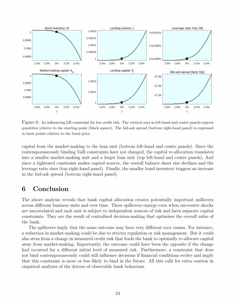
Relative efficiency governs the bank’s responses when an influencing LR constraint tightens,i.e. χ increases (Figure 8). Namely, a tightening of the constraint leads to a re-allocation of

13We verify that the tightening of any contemporaneously binding constraint has qualitatively similar implicationson dates 1 and 0. These results are available upon request.

14We focus on an influencing LR constraint, but note that the same reasoning applies to the case of an influencingVaR constraint.

23

2.6% 2.8% 3% 3.2% 3.4%

0.9985

0.999

0.9995

1Bond inventory: M

2.6% 2.8% 3% 3.2% 3.4%

1

1.00005

1.0001

1.00015

1.0002Lending volume: L

2.6% 2.8% 3% 3.2% 3.4%

3.61488%

3.61490%

3.61492%

Leverage ratio: K/(L+M)

2.6% 2.8% 3% 3.2% 3.4%

0.9985

0.999

0.9995

1

Market-making capital: Km

2.6% 2.8% 3% 3.2% 3.4%

1

1.0001

1.0002

Lending capital: Kl

2.6% 2.8% 3% 3.2% 3.4%

67.84

67.86

67.88

Bid-ask spread (bps): E[s]

Figure 8: An influencing LR constraint for low credit risk. The vertical axes in left-hand and centre panels expressquantities relative to the starting point (black square). The bid-ask spread (bottom right-hand panel) is expressedin basis points relative to the bond price.

capital from the market-making to the loan unit (bottom left-hand and centre panels). Since thecontemporaneously binding VaR constraints have not changed, the capital re-allocation translatesinto a smaller market-making unit and a larger loan unit (top left-hand and centre panels). Andsince a tightened constraint makes capital scarcer, the overall balance sheet size declines and theleverage ratio rises (top right-hand panel). Finally, the smaller bond inventory triggers an increasein the bid-ask spread (bottom right-hand panel).

6 ConclusionThe above analysis reveals that bank capital allocation creates potentially important spilloversacross different business units and over time. These spillovers emerge even when successive shocksare uncorrelated and each unit is subject to independent sources of risk and faces separate capitalconstraints. They are the result of centralised decision-making that optimises the overall value ofthe bank.

The spillovers imply that the same outcome may have very different root causes. For instance,a reduction in market-making could be due to stricter regulation or risk management. But it couldalso stem from a change in measured credit risk that leads the bank to optimally re-allocate capitalaway from market-making. Importantly, the outcome could have been the opposite if the changehad occurred for a different initial level of measured risk. Furthermore, a constraint that doesnot bind contemporaneously could still influence decisions if financial conditions evolve and implythat this constraint is more or less likely to bind in the future. All this calls for extra caution inempirical analyses of the drivers of observable bank behaviour.

24

ReferencesAdrian, T., Boyarchenko, N., Shachar, O., 2017. Dealer balance sheets and bond liquidity provision.

Journal of Monetary Economics 89, 92–109.

Adrian, T., Shin, H. S., 2011. Financial intermediary balance sheet management. Annual Reviewof Financial Economics 3, 289–307.

Armstrong, M., Vickers, J., 1991. Welfare effects of price discrimination by a regulated monopolist.The Rand journal of economics, 571–580.

Bank of England, July 2016. Financial stability report. Issue no 39.

Bao, J., O’Hara, M., Zhou, A., 2016. The Volcker rule and market-making in times of stress.Finance and Economics Discussion Series 2016-102, Board of Governors of the Federal ReserveSystem.

Baranova, Y., Liu, Z., Shakir, T., July 2017. Dealer intermediation, market liquidity and theimpact of regulatory reform. Staff Working Paper 665, Bank of England.

Baud, N., Frachot, A., Igigabel, P., Martineu, P., Roncalli, T., February 2000. An analysis frame-work for bank capital allocation. Discussion paper, Credit Lyonnais Research.

BCBS, November 2005. International convergence of capital measurement and capital standards.

BCBS, July 2009. Revisions to the Basel II market risk framework.

BCBS, June 2011. Basel III: A global regulatory framework for more resilient banks and bankingsystems.

BCBS, January 2014. Basel III leverage ratio framework and disclosure requirements.

BCBS, January 2016. Minimum capital requirements for market risk.

Begley, T. A., Purnanandam, A., Zheng, K., 2017. The strategic underreporting of bank risk.Review of Financial Studies 30 (10), 3376–3415.

Behn, M., Haselmann, R. F., Vig, V., July 2016. The limits of model-based regulation. ECBWorking Paper 1928, European Central Bank.

Cecchetti, S. G., Kashyap, A. K., November 2016. What binds? Interactions between bank capitaland liquidity regulations. Mimeo.

Chami, R., Cosimano, T. F., Ma, J., Rochon, C., February 2017. What’s different about bankholding companies? IMF Working Paper WP/17/26, International Monetary Fund.

Erel, I., Myers, S. C., Read, J. A., 2015. A theory of risk capital. Journal of Financial Economics118 (3), 620–635.

Fender, I., Lewrick, U., December 2015. Calibrating the leverage ratio. BIS Quarterly Review,43–58.

25

Froot, K. A., Stein, J. C., 1998. Risk management, capital budgeting, and capital structure policyfor financial institutions: an integrated approach. Journal of Financial Economics 47 (1), 55–82.

Garman, M. B., 1976. Market microstructure. Journal of Financial Economics 3 (3), 257–275.

Glosten, L. R., Milgrom, P. R., 1985. Bid, ask and transaction prices in a specialist market withheterogeneously informed traders. Journal of Financial Economics 14 (1), 71–100.

Gorton, G., Metrick, A., 2012. Securitized banking and the run on repo. Journal of FinancialEconomics 104, 425–451.

Guill, G. D., 2016. Bankers trust and the birth of modern risk management. Journal of AppliedCorporate Finance 28 (1), 19–29.

Ita, A., February 2016. Capital allocation in large banks – a renewed look at practice. SSRNWorking Paper.

James, C. M., 1996. RAROC based capital budgeting and performance evaluation: a case studyof bank capital allocation. Financial Institutions Center, The Wharton School, University ofPennsylvania.

Kyle, A. S., 1989. Informed speculation with imperfect competition. The Review of EconomicStudies 56 (3), 317–355.

Nishiguchi, K., Hiroshi, K., Takanori, S., October 1998. Capital allocation and bank managementbased on the quantification of credit risk. Economic policy review, Federal Reserve Bank of NewYork.

O’Hara, M., Oldfield, G. S., 1986. The microeconomics of market making. Journal of Financialand Quantitative analysis 21 (04), 361–376.

Perold, A. F., 2005. Capital allocation in financial firms. Journal of Applied Corporate Finance17 (3), 110–118.

Schmalensee, R., 1981. Output and welfare implications of monopolistic third-degree price dis-crimination. The American Economic Review 71 (1), 242–247.

Stein, J. C., 1997. Internal capital markets and the competition for corporate resources. TheJournal of Finance 52 (1), 111–133.

Stoughton, N. M., Zechner, J., 2007. Optimal capital allocation using RAROCTM and EVA R©.Journal of Financial Intermediation 16 (3), 312–342.

Tarashev, N., 2010. Measuring portfolio credit risk correctly: Why parameter uncertainty matters.Journal of Banking & Finance 34 (9), 2065–2076.

Wall, L. D., Peterson, D. R., 1987. The effect of capital adequacy guidelines on large bank holdingcompanies. Journal of Banking & Finance 11, 581–600.

Wells Fargo, 1974. Annual report – letter to shareholders. Wells Fargo & Company.

Zaik, E., Kelling, W. G., Retting, G., James, C., 1996. RAROC at Bank of America: from theoryto practice. Journal of Applied Corporate Finance 9, 83–93.

26

A Appendix

A.1 Business-unit LR constraintThe optimisation problem of the bank at date t ∈ 0, 1 is as follows:

Ut(Kt) = maxLt,Mt,Kmt,Klt

∆

E[Ut+1

(Vmt+1(Mt, Kmt; εt+1) + Vlt+1(Lt, Klt;Zt+1)

)]subject to

MRCLRmt ≡ χMt ≤ Kmt [ζLRmt ] (24)

MRCLRlt ≡ χLt ≤ Klt [ζLRlt ] (25)

MRCV aRmt ≡ RMt + ΩMt − F (Mt)

R≤ Kmt [ζV aRmt ] (26)

MRCV aRlt ≡ RLt + ΘLt −G(Lt)

R≤ Klt [ζV aRlt ] (27)

Kmt +Klt = Kt [ηt]where Ut is the value function, the bank’s capital stock, Kt, is the state variable and Lagrangemultipliers are in square brackets. Since the bank is risk-neutral, U2 is the identity function.

Suppose that the binding constraints for the loan and market-making units are i and j, respec-tively. We then obtain the feasibility condition

MRCimt +MRCj

lt ≤ Kt i, j ∈ V aR,LRand the first-order optimality conditions for the two units:

[Mt] : E[U ′t+1(.)∂Vmt+1

∂Mt

]− ζ imt

∂MRCimt

∂Mt

= 0

[Lt] : E[U ′t+1(.)∂Vlt+1

∂Lt

]− ζjlt

∂MRCjlt

∂Lt= 0.

Since capital is fungible between the two units, the Lagrange multipliers of the two binding con-straints are equal in equilibrium, ζ imt = ζjlt. Defining CRARs as in (16), it follows that they shouldbe equal across units:

E

[U ′t+1(.)∂Vmt+1

∂Mt

]/∂MRCi

mt

∂Mt︸ ︷︷ ︸CRARi

mt

= E

[U ′t+1(.)∂Vlt+1

∂Lt

]/∂MRCj

lt

∂Lt︸ ︷︷ ︸CRARj

lt

.

In the special case of no binding constraint, ζ imt = ζjlt = 0 and the bank equalises RARs, as definedin (15).

Note that MRCs increase in the size of the underlying unit: dMRCixt/dX > 0. For binding LR

constraints, this is seen immediately in expressions (24) and (25). For binding VaR constraints,expressions (26) and (27) reveal that MRC is a convex function of the unit size. Since this functionalso passes through the (0, 0) point, it is guaranteed to be increasing wherever size and MRC areboth positive (which is the only relevant case).

Note also that the date-1 CRAR decreases in the underlying unit’s size: dCRARixt/dX < 0.

This is the result of diminishing marginal returns, which make (i) marginal cash flows decrease inthe unit’s size – recall expressions (5) and (6) – and (ii) marginal MRC weakly increase in this size– see expressions (24) to (27).

27

A.2 Proof of Proposition 1.2Let x stand for the business unit whose binding constraint is tightened and let X stand for thisunit’s size. Conversely, let y and Y stand for the other business unit and its size. By proposition(1.1), the tightened constraint causes unit x to shrink: X < 0. In this appendix, we prove underwhat conditions the capital allocated to unit x, i.e. Kx, rises (drops), thus necessitating a drop(rise) in Ky and Y .

Consider two hypothetical responses of unit x to a tightening of its binding constraint. Namely,we denote by X|

MRCix< 0 and X|

CRARix< 0 the change in X that maintains the unit’s MRC –

respectively, CRAR – constant. Each of these changes is negative because, as proved in AppendixA.1 – dMRCi

x/dX > 0 and dCRARix/dX < 0.

Next, we show that the actual response, X, can be neither smaller nor larger than both of thesehypothetical responses.

• X < min(X|MRC

ix, X|

CRARix) < 0 leads to a contradiction. If this ordering held in equilib-

rium: (i) X < X|MRC

ix

would imply a drop in Kx; (ii) X < X|CRAR

ix

and dCRARix/dX < 0

would imply a rise in the CRAR of unit x. When Kx declines, Ky increases because the over-all capital is fixed and unit y was initially facing a binding constraint. Since this constraintdid not change, an increase in Ky implies a higher Y . But a higher Y and dCRARi

y/dY < 0imply a drop in the CRAR of unit y. In conjunction with (ii), this implies that the CRARsare not equal across business units. This cannot be an equilibrium.

• max(X|MRC

ix, X|

CRARix) < X < 0 also leads to a contradiction. The argument is symmetric

to the previous one, with all signs reversed and the conclusion still being that the CRARsare not equal across business units.

There are thus two possible orderings of the actual and hypothetical responses.

• X|MRC

ix< X < X|

CRARix< 0. In this case, X decreases by less than what is needed to

maintain the original MRC. Thus, the MRC increases and so must Kx for the tightenedconstraint to be satisfied.

• X|CRAR

ix< X < X|

MRCix< 0. In this case, a symmetric argument leads to the conclusion

that Kx declines.

The first ordering is a necessary and sufficient condition for unit x to be the more efficientone. When this ordering is in place, dCRARi

x/dX < 0 implies that the shrinkage of unit x thatmaintains the initial MRC also raises the CRAR above its initial level. Symmetrically, if thesecond of the two possible orderings is in place, the shrinkage of unit x that maintains the initialMRC also suppresses the CRAR below its initial level. Or, in terms of the notation introducedin Section 4.2, X|

MRCix< X|

CRARix

is equivalent to ∂CRARix/ ∂i+ (∂CRARi

x/ ∂X) X|MRC

ix> 0.

And since constraint i does not bind for unit y, it is trivially the case that ∂CRARjy

/∂i +(

∂CRARjy

/∂Y

) ·Y |

MRCjy

= 0. Thus, unit x satisfies the efficiency condition (17) if and only ifX|

MRCix< X|

CRARix.

Finally, we showed above that capital is re-allocated to unit x if and only if X|MRC

ix< X|

CRARix.

This proves Proposition 1.2.

28

A.3 Proof of Proposition 2.2Recall the equilibrium conditions:

G′(L)−Rχ = F ′(M)−R

χ (28)χM + χL = K (29)

Without loss of generality, let the lending unit be more efficient. Applying the definition ofefficiency (17) to equations (28) and (29) leads to:

−MF ′′(M) < −G′′(L)L. (30)

The goal is to show that Kl increases in response to a higher χ if and only if the latter inequalityholds. Total differentiation of equations (28) and (29) implies:

G′′(L)L = F ′′(M)M , (31)χL+ L+ χM +M = 0. (32)

And the solution of this system of equation delivers:

Kl = χL+ L = −MF ′′(M)− LG′′(L)F ′′(M) +G′′(L) ,

where the first equality follows from the definition Kl ≡ χL. Indeed, the last expression is positiveif and only if inequality (30) holds.

A.4 Bank-wide LR constraintIn this appendix, we show that both business units cannot shrink if the bank switches from abusiness-unit to a bank-wide LR constraint. In the first case, the constraint set is the intersectionof allocations that are feasible given the two VaR constraints and the two LR constraints:

C1 =

(L,M,Kl, Km) ∈ R4+ | Km +Kl = K; χL ≤ Kl; χM ≤ Km;

RL+ ΘL−G(L)R

≤ Kl;RM + ΩM − F (M)

R≤ Km

In the second case, the constraint set is the intersection of allocations that are feasible given thetwo VaR constraints and the single bank-wide LR constraint:

C2 =

(L,M,Kl, Km) ∈ R4+ | Km +Kl = K; χ(L+M) ≤ K;

RL+ ΘL−G(L)R

≤ Kl;RM + ΩM − F (M)

R≤ Km

We will first show that C1 ⊂ C2. To this end, consider an arbitrary point c = (L′,M ′, K ′l , K′m) ∈

C1. First, note that c satisfies the two VaR constraints, as they are common determinants ofC1 and C2. Second, note that since c satisfies χL′ ≤ K ′m and χM ′ ≤ K ′l , it trivially satisfiesχ(L′ +M ′) ≤ K = K

′m +K

′l . Therefore, any point in C1 belongs to C2 as well.

C1 ⊂ C2 implies that the maximum of the value function achieved under C2 is at least as highas that achieved under C1. Since this function is monotonically increasing in L and M , it thenfollows that L and M cannot be both smaller in the bank-wide LR regime.

29

Previous volumes in this series

No Title Author

665 October 2017

Interest rates and house prices in the United States and around the world

Gregory D Sutton, Dubravko Mihaljek and Agne Subelyte

664 October 2017

Is the price right? Swing pricing and investor redemptions

Ulf Lewrick and Jochen Schanz

663 October 2017

Liquidity risk in markets with trading frictions: What can swing pricing achieve?

Ulf Lewrick and Jochen Schanz

662 September 2017

The real effects of relationship lending Ryan N Banerjee, Leonardo Gambacorta and Enrico Sette

661 August 2017

How important is the Global Financial Cycle? Evidence from capital flows

Eugenio Cerutti, Stijn Claessens and Andrew K Rose

660 August 2017

Informal one-sided target zone model and the Swiss Franc

Yu-Fu Chen, Michael Funke and Richhild Moessner

659 August 2017

Effects of capital controls on foreign exchange liquidity

Carlos A Cantú García

658 August 2017

The distance effect in banking and trade Michael Brei and Goetz von Peter

657 August 2017

Quality pricing-to-market Raphael A Auer, Thomas Chaney and Philip Sauré

656 August 2017

Demographics will reverse three multi-decade global trends

Charles Goodhart and Manoj Pradhan

655 August 2017

The FinTech opportunity Thomas Philippon

654 August 2017

World changes in inequality: an overview of facts, causes, consequences and policies

François Bourguignon

653 August 2017

Dollar Pricing Redux Camila Casas, Federico Díez, Gita Gopinath and Pierre-Olivier Gourinchas

652 July 2017

The discontinuation of the EUR/CHF minimum exchange rate in January 2015: was it expected?

Michael Funke, Julius Loermann and Richhild Moessner

All volumes are available on our website www.bis.org.