Biosphere-atmosphere exchange of CO2 in relation to climate: a

Biogeosciences, 6, 2297–2312, 2009www.biogeosciences.net/6/2297/2009/© Author(s) 2009. This work is distributed underthe Creative Commons Attribution 3.0 License.

Biogeosciences

Biosphere-atmosphere exchange of CO2 in relation to climate: across-biome analysis across multiple time scales

P. C. Stoy1,2, A. D. Richardson3, D. D. Baldocchi4, G. G. Katul5, J. Stanovick6, M. D. Mahecha7,8, M. Reichstein7,M. Detto4, B. E. Law9, G. Wohlfahrt 10, N. Arriga 11, J. Campos12, J. H. McCaughey13, L. Montagnani14,15,K. T. Paw U16, S. Sevanto17, and M. Williams1

1School of GeoSciences, University of Edinburgh, Edinburgh EH9 3JN, UK2Department of Land Resources and Environmental Sciences, Montana State University, Bozeman, MT 59717-3120, USA3Department of Organismic and Evolutionary Biology, Harvard University, Cambridge, MA 02138, USA4Department of Environmental Science, Policy, and Management, University of California at Berkeley, Berkeley, CA, USA5Nicholas School of the Environment and Earth Sciences, Duke University, Box 90328, Durham, NC 27708, USA6USDA Forest Service, Northern Research Station, Newtown Square, PA 19073, USA7Max Planck Institute for Biogeochemistry, P.O. Box 10 01 64, 07701 Jena, Germany8Department of Environmental Sciences, ETH, 8092 Zurich, Switzerland9Department of Forest Science, Oregon State University, USA10Institut fur Okologie, Universitat Innsbruck, Austria11Department of Forest Science and Environment, University of Tuscia, 01100 Viterbo, Italy12Instituto Nacional de Pesquisas da Amazonia – INPA, Manaus, Brasil13Department of Geography, Queen’s University, Canada14Forest Service and Agency for the Environment, Autonomous Province of Bolzano, Bolzano, Italy15University of Bolzano/Bozen, Bolzano, Italy16Department of Land, Air, and Water Resources, University of California, Davis, USA17Department of Physics, P.O. Box 64, 00014 University of Helsinki, Finland

Received: 31 March 2009 – Published in Biogeosciences Discuss.: 14 April 2009Revised: 5 October 2009 – Accepted: 13 October 2009 – Published: 30 October 2009

Abstract. The net ecosystem exchange of CO2 (NEE) variesat time scales from seconds to years and longer via theresponse of its components, gross ecosystem productivity(GEP) and ecosystem respiration (RE), to physical and bi-ological drivers. Quantifying the relationship between fluxand climate at multiple time scales is necessary for a com-prehensive understanding of the role of climate in the ter-restrial carbon cycle. Orthonormal wavelet transformation(OWT) can quantify the strength of the interactions betweengappy eddy covariance flux and micrometeorological mea-surements at multiple frequencies while expressing time se-ries variance in few energetic wavelet coefficients, offeringa low-dimensional view of the response of terrestrial carbonflux to climatic variability. The variability of NEE, GEP andRE, and their co-variability with dominant climatic drivers,are explored with nearly one thousand site-years of data fromthe FLUXNET global dataset consisting of 253 eddy co-

Correspondence to:P. C. Stoy([email protected])

variance research sites. The NEE and GEP wavelet spectrawere similar among plant functional types (PFT) at weeklyand shorter time scales, but significant divergence appearedamong PFT at the biweekly and longer time scales, at whichNEE and GEP were relatively less variable than climate. TheRE spectra rarely differed among PFT across time scales asexpected. On average, RE spectra had greater low frequency(monthly to interannual) variability than NEE, GEP and cli-mate. CANOAK ecosystem model simulations demonstratethat “multi-annual” spectral peaks in flux may emerge at low(4+ years) time scales. Biological responses to climate andother internal system dynamics, rather than direct ecosys-tem response to climate, provide the likely explanation forobserved multi-annual variability, but data records must belengthened and measurements of ecosystem state must bemade, and made available, to disentangle the mechanismsresponsible for low frequency patterns in ecosystem CO2 ex-change.

Published by Copernicus Publications on behalf of the European Geosciences Union.

http://creativecommons.org/licenses/by/3.0/

2298 P. C. Stoy et al.: CO2 flux and climate spectra

1 Introduction

Variability in the global carbon cycle is dominated by ter-restrial ecosystem metabolism (Houghton, 2000; Canadellet al., 2007) and it is critical to understand how and whythe terrestrial carbon cycle varies to advance in our knowl-edge of the Earth system. The net ecosystem exchange ofCO2 (NEE) between the biosphere and atmosphere is deter-mined by the response of its components, gross ecosystemproductivity (GEP) and ecosystem respiration (RE) to physi-cal and biological drivers which vary at multiple time scales.Modeling and time series analysis of eddy covariance (EC)measurements of NEE have demonstrated that its variabilityis largely determined by physical (i.e. climatic) controls atshort controls at short (e.g. daily) time scales and by biolog-ical responses to climatic varaibility at longer (e.g. seasonaland interannual) time scales (Stoy et al., 2005; Richardsonet al., 2008). Process-based ecosystem models often experi-ence difficulties in replicating interannual variability in NEE(Siqueira et al., 2006; Urbanski et al., 2007), suggesting thatour knowledge of the carbon cycle at multiple time scalesmust improve.

Models synthesize our knowledge of terrestrial carbon ex-change and thus represent an explicit hypothesis about howecosystem function transfers variability in climatic forcingto an ecological response, namely the flux of mass or energy.These ecosystem transfer properties can now be explored us-ing long-term meteorological and carbon flux measurementsfrom the international FLUXNET project, which consists ofeddy covariance tower flux measurements from regional net-works [CarboeuropeIP, AmeriFlux, Fluxnet-Canada, LBA,Asiaflux, Chinaflux, USCCC, Ozflux, Carboafrica, Koflux,NECC, TCOS-Siberia, (e.g.,Aubinet et al., 2000; Baldoc-chi et al., 2001a; Baldocchi, 2008)]. The FLUXNET projectoffers the unprecedented opportunity to relate directly themeasured variability in mass and energy flux to the measuredmeteorological variability at time scales from hours to years,and in some cases over a decade (Grunwald and Bernhofer,2007; Urbanski et al., 2007; Granier et al., 2008).

Information on ecosystem properties (e.g. canopy N, leafarea index, vegetation growth) in the FLUXNET databaseis increasingly available, but currently lacking are measure-ments of how ecosystem properties change over time. Suchmeasurements are needed to synthesize how climate andecology interact to dictate NEE across time scales in globalecosystems. In spite of these limitations, our knowledge ofecosystem carbon cycling and its variability can be improvedby investigating the global relationships between observedclimate and plot-level biosphere-atmosphere fluxes acrosstime scales from hours to years.

Complicating efforts to understand the relationship be-tween flux and climate at multiple frequencies is the sizeof the FLUXNET database (Table1), inherent gaps in theeddy covariance measurement records (Falge et al., 2001),and nonstationarity in flux time series (Katul et al., 2001;

Scanlon and Albertson, 2001). Extracting patterns from theFLUXNET database to investigate multi-scale relationshipsbetween flux and climate requires a methodology that is ro-bust to data gaps and time-varying statistics that can simulta-neously decrease the magnitude of flux time series in the timescale domain. Orthornormal wavelet transformation (OWT)with the Haar wavelet basis function (Katul et al., 2001) isideally suited to mine (extract pattern from) flux data given:(i) the finite support and time locality of the Haar basis func-tion for removing the effects of data gaps on spectral andcospectral calculations on nonstationary time series and (ii)the data reduction properties of OWT.

Our objective is to quantify the spectral properties offlux time series and the cospectral relationships among fluxand climate in the FLUXNET database at time scales fromhours to multiple years to investigate the degree to whichbiosphere-atmosphere C flux can be explained by instanta-neous climate variability. This investigation contributes tomajor challenges in carbon cycle science including Ameri-Flux science question 3: “What is the causal link betweenclimate and the exchanges of energy, CO2 and water vaporfor major vegetation types, and how do seasonal and inter-annual climate variability and anomalies influence fluxes?”Given previous findings in temperate forest ecosystems (Stoyet al., 2005; Richardson et al., 2008), we anticipate that theinstantaneous effects of climate variability on flux variabilitywill diminish at seasonal to interannual time scales, when bi-ological changes that result from ecosystem development andecosystem response to abrupt and slow variations in local cli-mate dominate flux. Consequently, we hypothesize that themagnitude of the flux-climate cospectra will be lower at sea-sonal and annual time scales than daily time scales.

To accomplish our objectives and address the hypothe-sis, we quantify statistical differences among the spectra ofnet ecosystem exchange (NEE), gross ecosystem productiv-ity (GEP) and ecosystem respiration (RE) using 999 site-years of eddy covariance data from 253 ecosystems acrossthe globe in the FLUXNET database using OWT (Katul etal., 2001). After exploring the inherent variability in NEE,GEP and RE across time scales, we quantify: (1) ecosys-tem spectral transfer (EST), defined here as the simple ratiobetween the orthonormal wavelet power spectra of ecosys-tem response variables (in this case NEE, GEP and RE), andthe OWT spectra of different meteorological forcings, herephotosynthetic photon flux density (PPFD), air temperature(Ta), vapor pressure deficit (VPD), and precipitation (P); (seeFig. 1: Analysis I); (2) the wavelet co-spectra, which can beused to investigate the scale-wise correlations between cli-mate and flux (see Fig.1: Analysis II). In an appendix, wefurther investigate (3) 18 years of CANOAK model outputsto quantify the role of climate in driving interannual vari-ability in NEE, GEP and RE using Fourier decomposition(Baldocchi and Wilson, 2001).

Analysis I assesses the frequencies at which an ecosys-tem response modulates a given meteorological forcing via

Biogeosciences, 6, 2297–2312, 2009 www.biogeosciences.net/6/2297/2009/

P. C. Stoy et al.: CO2 flux and climate spectra 2299

Table 1. The number of FLUXNET research sites in version 2 of the LaThuille FLUXNET dataset with ecosystem type information, the totalnumber of site years of data, the number of potential 1/2 h eddy covariance flux measurements, and resulting number of wavelet coefficientsafter orthonormal wavelet transformation (OWT), with respect to the climate and vegetation classes investigated here (afterWilliams et al.,2009).

Crop Shrub+ DBF EBF ENF Grass MF Savanna− Wet Total Site-years Time series length∗ OWT coeff.

Temperate 17 0 8 2 12 18 4 0 4 65 255 4 470 473 932Temp.-Cont. 7 4 9 1 17 7 8 0 0 53 213 3 734 300 761Tropical 1 1 0 9 0 1 0 3 0 15 49 858 960 214Dry 0 1 0 1 1 3 0 4 0 10 27 473 280 153Boreal 0 4 2 0 22 4 2 0 4 38 161 2 822 782 549Arctic 0 0 2 0 0 1 0 0 3 6 22 385 678 86Subtrop.-Medit. 5 6 11 5 17 11 2 6 0 63 272 4768551 941

Total 30 16 32 18 69 45 16 13 11 250 999 17 514 024 3594Site years 79 50 149 77 340 135 74 58 37 999Length* 1 384 799 87 6576 2 612 253 1 349 902 5 961 015 2 366 735 1 297 342 1 016 684 648 718 17 514 024OWT coeff. 416 225 465 263 1010 636 235 188 156 3594

∗ Potential half-hour time series magnitude if measurements were continuous.+ Closed and open shrublands were combined.− Savanna and woody savanna were combined.

Crop=cropland/agricultural ecosystems. Shrub=shrubland ecosystems. DBF=Deciduous broadleaf forests. EBF=evergreen broadleafforests. ENF=evergreen needleleaf forests. MF=mixed forests. Grass=grassland. Wet=wetlands. Temp.-Cont.=Temperate-Continental.Subtrop.-Medit.=Subtropical-Mediterranean.

changes in state variables or functional parameters, and howthe frequencies of this modulation shift among climate andecosystem type. Analysis II is intended to unveil if scale-wise correlations between ecosystem responses and climaticvariables shift with respect to ecosystem type and climateregime to test the hypothesis. Analysis III explores low fre-quency flux variability. Results are discussed in the contextof the hypotheses and the implications for multi-scale eco-logical modeling of the terrestrial carbon cycle (Williams etal., 2009).

2 Methods

2.1 FLUXNET database

Flux and meteorological data from version 2 of the LaTh-uile FLUXNET database (www.fluxdata.org) was used. Datawere collected at individual sites according to network spe-cific protocols (e.g.,Aubinet et al., 2000), although devia-tions in methodology cannot be fully excluded for all sites.Half-hourly flux data were then processed according to theFLUXNET protocols. These include a filter for periodsof insufficient friction velocity (u∗), the despiking of half-hourly flux data (Papale et al., 2006), and the partition-ing of measured NEE into GEP and RE (Reichstein et al.,2005). FLUXNET products that fill the data gaps that re-sult from missing measurements are not used in the presentstudy, which investigates only measured flux and meteoro-logical data that have passed quality control checks. Theversion 2 database includes 253 research sites encompassing7 climate types and 11 vegetation types (Table1) (Cook et

al., 2007; Agarwal et al., 2007). To obtain sufficient samplesizes of different ecosystem types for the statistical analysis,the vegetation classes “savanna” and “woody savanna” werecombined to create one class called savanna, and the classes“open shrubland” and “closed shrubland” were combined tocreate one class called shrub. Data records extended fromseveral months to over a decade. The database currently con-tains over 17.5 million half-hourly data points for each vari-able, and over 18 billion total cells of information.

2.2 Orthonormal Wavelet Transformation (OWT)

A brief, qualitative description of wavelet methodology ispresented here; we refer the reader toTorrence and Compo(1998) for a basic treatment for geo-scientific applications,and Katul et al. (1995, 2001) for a detailed discussion ofwavelet analysis for flux applications.Scanlon and Albert-son(2001) andStoy et al.(2005) present conceptual descrip-tions of wavelet techniques and further examples of waveletanalysis for biosphere-atmosphere flux research.

Wavelet decomposition differs from standard Fourier tech-niques in that it employs a finite basis function, called a“mother wavelet”, that is translated (shifted) and dilated (ex-panded and contracted) across a signal to quantify, for thecase of a time series, signal variance across both time andtime scale. An infinite number of wavelet basis functionsexist given the admissibility criteria that its integral is zero(Daubechies, 1992). The choice between multiple waveletbasis functions for a given application may appear subjec-tive, but basis functions that are optimal for given time se-ries properties can and should be selected (Torrence andCompo, 1998). For the case of FLUXNET time series the

www.biogeosciences.net/6/2297/2009/ Biogeosciences, 6, 2297–2312, 2009

www.fluxdata.org


1

Forcing ResponseClimatic variability

MET=[Ta, VPD, PPFD, P…]

Ecosystem state: LAI(t), B(t), etc…

Analysis II: Wavelet cospectrumAnalysis I: Ecosystem Spectral Transfer

ENF

DBF

Flux variability

FLUX=[NEE, GEP, RE]

Grass

Arctic

MET

FLUXMETFLUX,

OWT

OWTlogEST =

Amplify

Dampen

Scale-wise correlations

Fig. 1. A conceptual description of the ecosystem transfer process from input (in this case climatic variability, upper left) to response (herethe net ecosystem exchange of CO2, NEE, upper right) as represented by the orthonormal wavelet spectrum of the respective time series(OWT). The response of NEE to climatic variability depends on ecosystem type; Arctic, deciduous broadleaf forest (DBF), grassland andevergreen needleleaf forest (ENF) ecosystems are shown as examples. Response to climatic variability also depends on ecosystem statethrough, for example, leaf area index (LAI) or biomass (B), both of which vary across time and space. This study introduces the ecosystemspectral transfer function (EST), defined as the ratio between the wavelet spectra of NEE and climatic drivers (Analysis I). A co-spectralanalysis to identify scale-wise correlations between climate and flux is performed in Analysis II.

Haar wavelet basis function (a square wave) is the most log-ical choice given its localization in the temporal domain andconsequent ability to control for the effects of the sharp dis-continuities created by the inherent gaps (Falge et al., 2001;Katul et al., 2001). In this way, scale-wise contributions tothe variance of the measured flux data can be quantified with-out considering the contributions of models to gapfill missingflux data, which are characterized by the frequency dynamicsof their underlying driving variables.

The wavelet transform can be continuous, but discretiza-tions that avoid redundant information to return a tractablenumber of coefficients are advantageous. Orthonormalwavelet transformation (OWT) features a log-spaced dis-cretization that quantifies the total variance of a time se-ries of length 2N in only N coefficients. For the case ofFLUXNET data, the response between climatic drivers andthe surface exchange of mass and energy for each measure-ment site across temporal scales can be expressed in terms oftens of wavelet coefficients that represent variability at dif-ferent scales in time (the “time scale domain”) rather than

tens to hundreds of thousands of data points in the tempo-ral domain (Katul et al., 2001; Braswell et al., 2005; Stoyet al., 2005; Richardson et al., 2007). The wavelet cospec-tra between driver and flux can also be quantified to explorescale-wise climate-flux correlations (Katul et al., 2001; Stoyet al., 2005) (see alsoSaito and Asunama, 2008).

We note that differences in the spectral estimate betweenFourier and wavelet based methods are expected given thatthe two techniques decompose data using fundamentally dif-ferent basis functions and algorithms. However, it shouldalso be emphasized there is no “true” spectrum for com-plex, finite time series; Fourier decomposition assumes thatthe time series is composed of a combination of sinusoidalcurves, which need not be the case. There is no reasonwhy two spectra obtained with different kernels should beidentical (Torrence and Compo, 1998). The only neces-sary requirement for spectral decomposition is conservationof spectral energy when summed across all frequencies (i.e.Parseval’s Identity,Dunn and Morrison, 2005), which OWTsatisfies. This is one reason why spectral scaling exponents



inferred from OWT and Fourier methods agree reasonablywell and are insensitive to the choice of the basis functionwhen the time series exhibits an extensive scaling law acrossa wide range of scales (Katul and Parlange, 1994).

To compute OWT coefficients, all half-hourly measure-ments of NEE, GEP, RE,Ta , VPD, PPFD,P and latent heatflux (LE) in the FLUXNET database were multiplied by theirquality control flag (1 for raw data, 0 for missing data) to ex-clude missing or gapfilled measurements (Stoy et al., 2005).This treatment ensured that data gaps do not contribute to thetotal series variance after Haar wavelet decomposition. Alltime series were then normalized to have zero mean (withzeroes in place of gaps) and unit variance for comparison.The time series for each site then underwent a standard “zero-padding” (Torrence and Compo, 1998) by adding zero valuesto both ends of the time series in order to make the lengthof each time series equal to a power of 2 for fast waveletdecomposition. The resulting zero-padded series was thenagain normalized to ensure that the normalized time serieshave unit variance and that all periods without valid mea-surements were set to zero. Differing lengths of the fluxdata records resulted in 15–18 dyadic scale representationsper site and data record. The lowest-frequency wavelet coef-ficient for each normalized time series is poorly constrainedand was dropped from the analysis, resulting in a maximumtime scale of 217 half hours, or 7.48 years for the 16 yearHarvard Forest time series.

For simplicity, orthonormal wavelet coefficients for allflux time series (NEE, GEP and RE) are abbreviatedOWTFLUX , all meteorological time series are abbreviatedOWTMET and some combination of flux and meteorologi-cal drivers are abbreviated OWTX. For the purposes of thisinvestigation, LE is often considered alongside the meteo-rological drivers to investigate the coupling between carbonand water fluxes.

The ecosystem spectral transfer (EST) can be defined as

ESTFLUX,MET = logOWTFLUX

OWTMET. (1)

The flux signal is said to be “amplified” (“dampened”) com-pared to the respective climatic input if ESTFLUX,MET is pos-itive (negative) (Fig.1: Analysis I). We note that conceptsand terminology from the signal processing literature, “am-plifying”, “dampening”, “modulating”, and “resonating” finda natural application when discussing eddy covariance mea-surements because the flux and meteorological variables aretime-varying signals and ecosystems can be thought to pro-cess this signal in a corresponding, time-varying response(Fig. 1). Amplification or dampening need not imply causal-ity in systems, like ecosystems, that respond to a range offactors; rather, the EST is investigated to ascertain the sim-plest possible description of the instantaneous response ofecosystems to climate across scales of time.

To investigate how climatic inputs and flux outputs co-resonate and to test the hypothesis, we quantified the wavelet

Fig. 2. Orthonormal wavelet power spectra of normalized netecosystem exchange (OWTNEE), normalized gross ecosystemproductivity (OWTGEP) and normalized ecosystem respiration(OWTRE) for the 253 eddy covariance sites in version 2 of theFLUXNET database after transformation using the Haar waveletbasis function. The white bars represent the median of the dis-tribution of wavelet coefficients at each time scale, and the thickvertical bars encompass the interquartile range. Outliers are ex-pressed as dots outside the thin vertical bars, which represent 1.5×

the interquartile range. The GEP and RE spectra have been shiftedto avoid overlap for visualization. Circles at 71

2 years are for theHarvard Forest time series, which began in 1991. The numbersat the bottom of the plot represent the number of sites analyzedat each time scale; some sites have longer data records and there-fore a greater number of wavelet coefficients. Text at the top ofthe figure refers to the expressions and abbreviations for the dif-ferent time scales used throughout the manuscript. M.-Day=Multi-Day; Wk.=Weekly; Bi-W.=Bi-Weekly; Mo.=Monthly; Bi-M.=Bi-Monthly; Seas.=Seasonal.

covariance (Torrence and Compo, 1998) for all flux and me-teorology combinations, and abbreviate the resulting coeffi-cients OWTFLUX,MET Fig. 1: Analysis II). It is important tonote that OWTNEE,MET and OWTGEP,MET will be negative ifthe relationship between flux and meteorological variabilityis positive due to the micrometeorological sign conventionwhere flux from atmosphere to biosphere is denoted as neg-ative.

2.3 Statistical analyses

A mixed model (PROC MIXED in SAS 9.1) wasimplemented to test for differences among OWTFLUX ,ESTFLUX,MET, and OWTFLUX,MET for different climate andvegetation classes for the 250 of 253 FLUXNET sites withclimate and vegetation information. Wavelet variances werelog-transformed prior to analysis when necessary to en-sure normality of the response variables, noting that EST



is computed from log-transformed coefficients (Eq. 1). Co-efficients at the 3.74 year and 7.48 year time scales werenot included in the statistical analysis because the variablelength of the flux data records resulted in a smaller sam-ple size at low frequencies (see Fig.2). Time scale, climatetype, and PFT were specified as fixed main effects, and timescale×climate and time scale×vegetation were included asinteraction effects. The vegetation×climate interaction ef-fect was not included because of the large number of un-replicated combinations (Table1). Observations for each siteat different time scales were considered repeated measures,and a first-order autoregressive covariance structure was em-ployed. Overall least-square means were calculated for themain effects climate and vegetation. The Tukey-Kramer mul-tiple comparison test was used to evaluate overall differencesamong effect levels. We also tested for simple interaction ef-fects among climate and vegetation (“sliced”) per time scaleusing the PROC MIXED procedure in SAS 9.1. Test statis-tics that are significant at the 95% confidence level are re-ported.

3 Results

3.1 Variability in NEE, GEP and RE

Medians and ranges of OWTFLUX for all FLUXNET sites arepresented in Fig.2. Abbreviations (“hourly”, “daily”, “an-nual”, etc.) are used to approximate the discrete time scalesfor simplicity; for example, the annual coefficients representvariability at 0.935 years, daily coefficients represent 16 hvariability as 24 is not a power of 2, and “multi-day” rep-resents 1.33 day and 2.67 day variability because these timescales are longer than 1 day yet shorter than 1 week (Fig.2,see also Table2). These descriptions are meant to present asimple and intuitive means of communicating temporal scalefor interpreting results and are used subsequently. It shouldbe noted that sampling every third data point (1.5 h) wouldhave resulted in OWT coefficients at exactly 24 h, but theannual variability would be poorly resolved given that coef-ficients at 256 and 512 days would also be returned.

Local reductions in OWTFLUX power spectra (the so-called “spectral gaps”) exist at hourly time scales, and atmulti-day to bi-monthly time scales. A low frequencyspectral gap begins to appear at interannual time scales inOWTNEE and OWTGEP; less so in OWTRE (Fig. 2). NEEand GEP variability were, on average, relatively lower atthese time scales than the corresponding spectral peaks atdaily and seasonal/annual time scales. The relative differ-ence in OWTRE among sites increased at the longest timescale for which there were replicates (3.74 y), while inter-sitedifferences in OWTNEE and OWTGEP decreased at low fre-quencies (Fig.2). In other words, RE variability among siteswas more different at interannual time scales, while seasonaland annual variability in NEE and GEP were more different

among sites than RE. The single site with sufficient time se-ries length to identify 7.48 y variability, Harvard Forest, hadrelatively high flux variability in GEP and RE at these “multi-annual” time scales compared to the average 3.74 y interan-nual variability of other ecosystems.

3.2 Flux variability by climate zone and plantfunctional type

OWTFLUX (Fig. 2) was separated by climate and vegetationtype (Fig.3). Time scales for which there were significantdifferences among climate or vegetation types at the 95%confidence level, as determined by the multiple comparisontests, are listed in Table2 and also demarcated by the hori-zontal bars in Fig.3. (We note again that significance at thetwo lowest frequency time scales, 3.74 and 7.48 years, couldnot be determined due to lack of replicates.)

There were no significant differences in OWTNEE amongclimate zones at hourly to weekly time scales, and amongPFT at hourly (2 h) to bi-weekly time scales. This impliesuniversality in the total relative variability, but not magni-tude, of NEE at these time scales in the FLUXNET database.OWTGEP differed among climate types at bi-monthly to an-nual time scales, and among PFT at high-frequency (hourly)time scales and also monthly to seasonal time scales. Highfrequency (hourly to daily) OWTRE differed among climatetypes, but lower-frequency differences were only found atthe seasonal time scale. PFT-related differences in OWTREemerged at seasonal to interannual frequencies (Table2,Fig. 3).

3.3 Analysis I: spectra of meteorological drivers andecosystem responses

The median normalized power spectra of the flux and mete-orological drivers varied by orders of magnitude across timescales (Fig.4), highlighting the temporal dynamics of mi-croclimate at characteristic frequencies and subsequent veg-etation/ecosystem response via carbon flux (Baldocchi andWilson, 2001; Baldocchi et al., 2001b; Katul et al., 2001).Median OWTTa and OWTLE were notably energetic at sea-sonal and annual time scales. OWTP tended to be roughlyequal across time scales larger than the isolated storm timescale, approximating white-noise, consistent with other stud-ies (Katul et al., 2007; Mahecha et al., 2008); P is knownto possess a composite spectrum with multiple scaling lawsacross various frequencies (Gilman et al., 1963; Fraedrichand Larnder, 1993; Peters et al., 2002). The magnitudeof OWTGEP, OWTRE and OWTLE at Harvard Forest at the7.48 y time scale was large in comparison to FLUXNET me-dian flux interannual variability at the 1.87 and 3.74 y timescales (Figs.3 and4).



10−4

10−2

100

10−2

100

102

104

OW

T NE

E

Climate

10−4

10−2

100

10−2

100

102

104

Vegetation

10−4

10−2

100

10−2

100

102

104

OW

T GE

P

10−4

10−2

100

10−2

100

102

104

10−4

10−2

100

10−2

100

102

104

Time Scale (y)

OW

T RE

10−4

10−2

100

10−2

100

102

104

Time Scale (y)

TemperateTempContTropicalDryBorealArcticSTropMedit

CropShrubDBFEBFENFMFGrassWetland

Fig. 3. Mean wavelet spectra of the normalized net ecosys-tem exchange of CO2 (OWTNEE), gross ecosystem productiv-ity (OWTGEP), and ecosystem respiration (OWTRE) per climate(left-hand panels) and vegetation type (right-hand panels) for the250 eddy covariance measurement sites with ecosystem-level infor-mation in version 2 of the LaThuille FLUXNET database. Hor-izontal lines demarcate time scales at which there are significantdifferences among climate (top of subplot) or vegetation type (bot-tom of subplot) at the 95% significance level (see Table 2). Sig-nificance at the longest time scales (3.74 and 7.48 y) could not bedetermined among climate types due to lack of replicates. Circles atthe 7.48 year time scales represent flux variability at Harvard Forest.

The tendency of ecosystems to dampen or amplify thevariability of climatic drivers was explored via EST (Figs.1and 5). Figure 5 displays the median EST for eachflux/meteorological driver comparison. At hourly time scaleswhere flux footprint variability is known to dominate themeasurement signal in spatially heterogeneous ecosystems(Oren et al., 2006), the variability of NEE tended to begreater than that ofTa and VPD, but not PPFD. NEE andGEP were on average less variable than PPFD at time scalesgreater than an hour and shorter than a day, consistent withthe observed saturating response of GEP to PPFD. NEE andGEP were damped with respect toTa and VPD variabilityat weekly and longer time scales, on average (Fig.5a and b),

Table 2. Results from the mixed model analysis for significant in-teraction effects between meteorology (MET) by time scale (TS),and plant functional type (PFT) by TS on net ecosystem exchange(NEE) gross ecosystem productivity (GEP) and ecosystem respira-tion (RE) variability. Time scales for which spectra are significantlydifferent at the 95% confidence level are denoted by the flux termabbreviation. These significant interaction effects are presented asbars in Fig. 3 and this convention is kept in subsequent figures.

Time scale Time scale Description MET×TS PFT×TS(h)∗

214 1.87 years Interannual - NEE, RE213 0.935 years Annual NEE, GEP NEE, RE212 170.67 days Seasonal NEE, GEP NEE, GEP, RE211 85.33 days Seasonal NEE, GEP, RE NEE, GEP210 42.67 days Bi-Monthly NEE, GEP NEE, GEP29 21.33 days Monthly NEE NEE, GEP28 10.67 days Bi-Weekly NEE -27 5.33 days Weekly - -26 2.66 days Multi-day - -25 1.33 days Multi-day - -24 16 hours Daily RE -23 8 hours Hourly RE -22 4 hours Hourly RE -21 2 hours Hourly RE GEP20∗ 1 hour Hourly RE NEE, GEP, RE

∗ Eddy covariance-measured fluxes are calculated on the half-hourly basis. The highest frequency time scale considered is 21 halfhours=1 h.

but variability in RE was on average similar to or greater thanTa variability at time scales of weeks and longer (Fig.5c).Median OWTNEE was most similar to OWTPPFDacross timescales as evidenced by the near-zero scale-wise ESTNEE,PPFD(see also Fig.4), but at lower (monthly to annual) frequen-cies, OWTGEPwas most similar to OWTVPD (Figs.4, 5a and5b). OWTRE was most similar to OWTTa across time scales,but was also surprisingly similar to the median OWTLE spec-tra.

As a whole, ESTGEP,MET followed similar scale-wisepatterns to ESTNEE,MET (Fig. 5a and b), but medianESTNEE,MET was dampened to a greater degree, on average,at lower frequencies. Conversely, ESTRE,MET was amplifiedcompared climatic variability, on average, at the lower fre-quencies.

ESTFLUX,MET was significantly different among climatetype and PFT across a complex array of time scales withdistinct patterns, as demonstrated by the horizontal bars inFig. 5, noting again that the bars in the upper sections ofthe subplot demarcate significant differences among climatetype and the bars in the lower sections of the subplots signifysignificant differences among PFT. Slicing by climate typereveals significant differences at both short and long timescales in the relationship between all flux and meteorolog-ical variability. Significant differences among PFT emergedat longer (seasonal to annual) time scales in ESTNEE,MET andESTGEP,MET, less so ESTRE,MET.



Fig. 4. Median normalized orthonormal wavelet spectra of netecosystem exchange of CO2 (OWTNEE), gross ecosystem produc-tivity (OWTGEP), ecosystem respiration (OWTRE), latent heat ex-change (OWTLE) and the meteorological drivers air temperature(OWTTa

), photosynthetic photon flux density (OWTPPFD), vaporpressure deficit (OWTVPD) and precipitation (OWTP ). Points atthe 7.48 year time scale represent flux variability at a single site,Harvard Forest.

3.4 Analysis II: wavelet cospectra between NEE and cli-matic drivers

The covariance between flux and climate was dominatedby variability at daily and seasonal/annual time scales, butthe magnitude of this covariance tended to be greater atdaily rather than seasonal/annual time scales (Fig.6). MeanOWTNEE,Ta (i.e. the wavelet covariance between NEE andTa) at the seasonal and annual time scales for different cli-mate types were often of the same magnitude as those at thedaily time scale, in contrast to OWTNEE,LE, OWTNEE,VPD,and OWTNEE,PPFD, which had a greater magnitude, on av-erage, at daily time scales than seasonal or annual timescales (Fig.6a). OWTGEP,LE was on average larger at sea-sonal/annual time scales than at daily time scales, and themedian OWTRE,LE was unexpectedly large across monthlyto annual frequencies.

Despite the relatively low OWTFLUX,MET magnitude at in-terannual time scales, these cospectra are in almost all casessignificantly greater than that of a random signal at the 95%confidence level, as determined by a Monte Carlo analysiswith 1000 synthetic autoregressive pink noise time seriesof the sort commonly applied in geoscientific studies (e.g.,Allen and Smith(1996), see alsoRichardson et al.(2008),data not shown).

Most of the statistically-significant differences inOWTFLUX,MET among climate type and PFT were clusteredaround the daily and seasonal/annual spectral peaks, where

10−4

10−3

10−2

10−1

100

101

−6

−4

−2

0

2

4

6

ES

TN

EE

,ME

T

10−4

10−3

10−2

10−1

100

101

−6

−4

−2

0

2

4

6

ES

TG

EP

,ME

T

10−4

10−3

10−2

10−1

100

101

−6

−4

−2

0

2

4

6

ES

TR

E,M

ET

Time Scale (y)

ESTNEE,PPFD

ESTNEE,Ta

ESTNEE,VPD

ESTNEE,P

ESTNEE,LE

ESTGEP,PPFD

ESTGEP,Ta

ESTGEP,VPD

ESTGEP,P

ESTGEP,LE

ESTRE,PPFD

ESTRE,Ta

ESTRE,VPD

ESTRE,P

ESTRE,LE

Fig. 5. (Top) The mean difference between the log of the meteoro-logical drivers or latent heat exchange and NEE (i.e. the ecosystemspectral transfer function, ESTNEE,MET, Eq. 1), GEP (middle) andRE (bottom) for all sites in version 2 of the LaThuile FLUXNETdatabase. For example, in the top panel, NEE is more variable than(amplifies) climate variability if values are positive and damps cli-mate variability if values are negative. Horizontal lines demarcatetime scales at which there are significant differences among climate(top of subplot) or vegetation type (bottom of subplot) at the 95%significance level after Fig. 3. Points at the 7.48 year time scalerepresent flux variability at Harvard Forest.

most of the energy in the cospectra resides (Fig.6). No sig-nificant differences in the interaction effects among cospectrasliced by climate or PFT emerged at the weekly/monthlytime scales. There were significant differences at the diurnaltime scale when separating by both climate type and PFT forOWTNEE,MET and OWTGEP,MET, and significant differencesat the seasonal and annual time scales among both climatetype and PFT for all OWTNEE,MET and OWTGEP,MET exceptthe PPFD cospectra. There were no PFT-related differencesat hourly to seasonal time scales in OWTRE,Ta ; significantclimate and PFT-related differences for all OWTRE,METemerged only at seasonal to annual time scales.



10−4

10−3

10−2

10−1

100

101

−0.4

−0.2

0

0.2

0.4

OW

T NE

E,X

10−4

10−3

10−2

10−1

100

101

−0.3

−0.2

−0.1

0

0.1

OW

T GE

P,X

10−4

10−3

10−2

10−1

100

101

−0.1

0

0.1

0.2

0.3

OW

T RE

,X

Time Scale (y)

OWTNEE,PPFD

OWTNEE,Ta

OWTNEE,VPD

OWTNEE,P

OWTNEE,GPP

OWTNEE,RE

OWTNEE,LE

OWTGEP,PPFD

OWTGEP,Ta

OWTGEP,VPD

OWTGEP,P

OWTGEP,RE

OWTGEP,LE

OWTRE,PPFD

OWTRE,Ta

OWTRE,VPD

OWTRE,P

OWTRE,LE

Fig. 6. The median wavelet cospectra between (top) normalizednet ecosystem exchange of CO2 (NEE), (middle) gross ecosystemproductivity (GPP), and (bottom) ecosystem respiration (RE) andnormalized latent heat exchange (LE), meteorological drivers, andother flux terms (“X”) for all sites in version 2 of the LaThuileFLUXNET database. Negative cospectra indicate correlation be-tween climate and CO2 uptake given the meteorological conventionwhere C input into the biosphere is denoted as negative. Horizon-tal lines demarcate time scales at which there are significant dif-ferences among climate (top of subplot) or vegetation type (bottomof subplot) at the 95% significance level after Fig. 3. Points at the7.48 year time scale represent flux variability at Harvard Forest.

4 Discussion

4.1 Multi-scale flux variability across global ecosystems

Spectral peaks at daily and seasonal/annual time scales area general feature of the global NEE time series (Figs.2and3). These peaks have been quantified previously in tem-perate forested ecosystems (Baldocchi et al., 2001b; Katulet al., 2001; Braswell et al., 2005; Stoy et al., 2005; Mof-fat et al., 2007; Richardson et al., 2007) and further empha-size the dominant role of orbital motions at diurnal and sea-sonal/annual time scales in controlling the total variability inmeasured flux time series. Naturally, resolving such multi-

scale variability alone does not necessarily translate to accu-rate estimation of long-term mean flux.

These findings suggest that flux variability is concen-trated in few time scales, i.e. the spectra are “unbalanced”(Katul et al., 2007). It has been previously argued that low-dimensional ecosystem models that capture these dominantmodes of variability are a logical way forward for modelingflux at multiple time scales (Katul et al., 2001), but accu-rately modeling the seasonal and annual variability of fluxeshas proven elusive for ecosystem models (Hanson et al.,2004; Siqueira et al., 2006), in part because of the shift fromphysical to biological control at longer time scales (Stoy etal., 2005; Richardson et al., 2007) as also evidenced by thePFT-related differences in OWTFLUX at longer time scales(Fig. 3). For example, a series of drought years can lead toa carry-over effect of reduced carbohydrate reserves for treegrowth and a shift in carbon allocation in subsequent years,and incorporating these processes into ecological models iscomplex. Such dynamics were detailed at a semi-arid pinesite in which NEE was much lower in a third year of droughtthan the previous years, suggesting a cumulative effect ofecosystem biology on biosphere-atmosphere flux (Thomas etal., 2009).

It was found that the magnitude of the NEE and GEP spec-tra are not statistically different among climate zones or PFTuntil bi-weekly to monthly time scales are reached (Fig.3).In other words, PFT is not a logical way to separate differ-ences in the variability of flux time series at high frequenciesin the FLUXNET database, at least when quantifying the to-tal time series variance across scale rather than the changesin variance across scale and season. PFT does, however, sep-arate the variability in observed NEE and GEP at the lower(monthly and longer) frequencies that are arguably more im-portant for quantifying the role of terrestrial ecosystems inthe global carbon cycle.

Climate and PFT-related differences in the RE spectra donot emerge until seasonal time scales (Fig.3b). Given theability of the eddy covariance system to resolve RE, PFT isnot a logical way to separate RE variability across most ofthe time scales investigated here as expected. Because no sta-tistically significant spectral differences emerge among PFTat higher frequencies, it may be argued that PFT is a scale-dependent concept when considering the variability of fluxin response to climate, and models may be simplified by ig-noring vegetation-type distinctions at higher frequencies de-pending on the application and goals of the modeling analy-sis.

Regarding interannual and multi-annual flux variability,the 7.48 y variability in GEP and RE at Harvard Forest isgreater than climatic variability (Fig.4) and reflects the in-crease in flux magnitude over the course of measurementsrelated to the species compositional shift toward red maplecoupled with multi-annual recoveries from ecosystem distur-bance (Urbanski et al., 2007). Such increases in variability atthe low frequencies have been observed in other ecosystems



(Stoy et al., 2005; Richardson et al., 2007; Mahecha et al.,2008), but a comprehensive synthesis of disturbance eventson ecosystem C cycling requires more long term measure-ments from more ecosystems.

4.2 Ecosystem spectral transfer

Ecosystem CO2 uptake strongly dampened the variability ofmost climatic drivers, on average (i.e. average ESTNEE,METand ESTGEP,MET are less than zero) at time scales fromweeks to years (Fig.5), but ecosystem CO2 loss was ob-served to be more variable than climatic drivers at these lowerfrequencies (i.e. average ESTRE,MET>0). These results sup-port a homeostatic mechanism in which ecosystem CO2 up-take dampens instantaneous low frequency meteorologicalvariability (see, for example,Odum, 1969), but low fre-quency amplification of climate by RE does not. Rather, cli-matic variability “excites” the RE spectra on average, whichis consistent with the exponential transfer function com-monly used to model RE variability at high frequencies andthe strong spectral covariance between RE andTa at low fre-quencies (Figs.5c and6c). Also, significant differences inESTRE,MET emerged among different climate types, ratherthan PFT, across time scales (Fig.5c). Together with find-ings from the previous subsection, these results agree withthe notion that RE is determined by the effects of climateand moisture, more so than ecosystem type, on ecosystemC pools with different time scales of input and loss (Partonet al., 1987; Adair et al., 2008) despite the known couplingbetween GEP and RE (Hogberg et al., 2001; Ryan and Law,2005).

4.3 Cospectral relationships between flux and climate

Spectral peaks in NEE at longer (seasonal/annual) timescales are less-related to environmental drivers than the diur-nal spectral peak (Fig.6), which demonstrates a decreasinginstantaneous influence between climate and NEE at longertime scales globally (Richardson et al., 2007). Hence, it isno surprise that ecological models that use highly resolvedPPFD variability (i.e. hourly), and to a lesser extent VPDvariability, can explain the high-frequency energetic modesin NEE variability (Siqueira et al., 2006). At longer timescales, explaining flux variability via climatic variables aloneis no longer effective (Siqueira et al., 2006; Richardson et al.,2007; Stoy et al., 2008), in part because NEE and GEP tendto dampen climatic variability at low frequencies, supportingthe homeostatic mechanism discussed in classic studies likeOdum(1969). Results here agree with previous studies thathave found a shift from exogenous to endogenous control ofNEE in temperate deciduous broadleaf (DBF) and evergreenneedleleaf (ENF) forests (Baldocchi et al., 2001b; Stoy et al.,2005; Richardson et al., 2007). Quantifying flux variabilityat longer time scales requires information on how ecosys-

temschangein response to climatic variability, rather thanhow they merely respond to climatic variability.

4.4 Implications for ecological modelling

Significant climate and PFT differences in ESTFLUX,MET ap-peared across more time scales than significant differences inOWTFLUX,MET, which are primarily restricted to diurnal andseasonal/annual time scales (Figs.5 and6). To the extent thatchanges in EST represent a change in the state variables orparameters that transfer climatic input to ecosystem output(Fig. 1), these state variables, parameters, and their variabil-ity are often different among PFT at bi-weekly to monthlytime scales for NEE and GEP. Few PFT-related differencesin ESTRE,MET are significant, which again demonstrates thatincluding PFT is less important for modeling multi-scale RE(see also Fig.3). More ecosystem level ancillary data is re-quired to determine how the shifts in transfer properties resultfrom changes in ecosystem carbon stocks and/or the parame-ters of photosynthesis and respiration models (Wilson et al.,2001; Palmroth et al., 2005) to further investigate low fre-quency biological controls on flux (Richardson et al., 2007).An emerging challenge is to model the multi-annual spectralenergy of GEP and RE which, when combined via NEE, re-sults in a low frequency dampening of carbon sequestrationwith respect to climatic variability.

The significant variation of EST across time scale indi-cates that the representation of ecosystems as simple instan-taneous physical transformers, e.g. in simple soil-vegetation-atmosphere models (SVATs) for photosynthesis, or time in-variant regression equations for ecosystem respiration, islikely to fail at longer time scales (Carvalhais et al., 2008).This study confirms and generalizes former site-specificstudies that have shown that biological variation in space andtime is an important control of fluxes and may be empiri-cally represented by changing biological ecosystem param-eters that define the properties of the system (Wilson et al.,2001; Reichstein et al., 2003; Hibbard et al., 2005; Owenet al., 2007). In ecosystem process models, such temporaldynamics, which can change the response to climate vari-ables across time-scales, may be represented by state vari-ables (e.g. leaf area index, soil water content) and the ap-propriate representation of these state variables is pivotal formodeling NEE correctly across time scales, including poolsof soil carbon with slow turnover times (Adair et al., 2008).Moreover, whether biophysical and ecophysiological param-eters may be kept constant as is often the case in typical ter-restrial biosphere models employed at global scale, or if pa-rameters should be made temporally dynamic is a critical is-sue for modeling the land-surface C cycle (Curiel Yuste et al.,2004; Palmroth et al., 2005; Ryan and Law, 2005; Davidsonand Janssens, 2006; Juang et al., 2008; Williams et al., 2009).Modeling or measuring rapid transients in endogenous vari-ables (e.g. green-up of LAI in deciduous forests) may be crit-ical for explaining flux variability over the stochastic weekly-



monthly spectral gap in some ecosystems (Stoy et al., 2005).The importance of endogenous variables compared to cli-mate drivers might well be one general reason why remotesensing based approaches that incorporate the biophysicalstate of the vegetation are comparably successful in quantify-ing terrestrial productivity, even after completely abandoningthe use meteorological drivers (Jung et al., 2008).

A major motivation for the present study is to investigatethe multi-scale coupling between climate, hydrology and car-bon flux to identify potential improvements in ecosystemC models at the longer time scales at which they often fail(Hanson et al., 2004; Siqueira et al., 2006). The strong sea-sonal and annual OWTGEP,LE suggests that improving therepresentation of ecosystem hydrology and its coupling toCO2 uptake is a logical step to improve models of CO2 flux(Katul et al., 2003) in globally-distributed ecosystems. In-terestingly, the mean seasonal/annual OWTGEP,VPD was ofgreater magnitude than OWTGEP,PPFD (Fig. 5b), further em-phasizing the importance of hydrology in addition to radia-tion in determining the low frequency variability of photo-synthesis.

4.5 Multi-scale coupling between GEP and RE

Quantifying the coupling between photosynthesis andecosystem respiration has gained attention given that iso-topic and ecosystem manipulation studies have consistentlydemonstrated a strong daily-to-monthly coupling betweenCO2 input and output (Hogberg et al., 2001; Barbour et al.,2005; Taneva et al., 2006). Despite the known limitation ofthe artificial correlation between GEP and RE in eddy covari-ance measurements (Vickers et al., 2009) [but seeLasslopet al. (2009)], some evidence for their coupling across timescales may be gleaned from a conservative investigation oftheir co-spectral properties.

The magnitude of the instantaneous GEP-RE covariance(OWTGEP,RE) is large at seasonal to annual time scales; thisrelationship is on average as strong as the seasonal covari-ance between CO2 uptake and water loss (Fig.6). The GEP-RE covariance is also larger, on average, than the covariancebetween GEP and most meteorological drivers investigated,and is of the same average order of magnitude as OWTGEP,LEand OWTGEP,Ta . GEP has been shown to explain 89% of theannual variance of RE across FLUXNET (Baldocchi, 2008)despite site-by-site differences in the strength of this rela-tionship (Stoy et al., 2008). Formally linking GEP and REvariability in models at lower frequencies is a logical step forimproving model skill given the large low-frequency covari-ance between these fluxes, noting that the degree to whichGEP and RE are coupled at low frequencies versus the de-gree to which they are controlled by similar environmen-tal drivers across ecosystems remains unclear (Reichstein etal., 2007b). Future studies should investigate forthcomingFLUXNET data products that seek to minimize artificial cor-relations between GEP and RE (Lasslop et al., 2009).

Interestingly, the average seasonal/annual covariance be-tween RE and LE is as strong, or stronger, than the covari-ance between RE andTa . This may partly be explained bythe tight coupling of photosynthesis, transpiration, and rootrespiration during the growing season (Drake et al., 2008).A strong correlation was observed between tree transpiration(sapflow) and root respiration measured on individual iso-lated trees at the semi-arid Metolius site, and soil respirationdeclined with soil water deficit as soil temperature continuedto increase (Irvine et al., 2008) (see alsoTang et al., 2005).The mechanisms for this relationship in the global databaseare less clear, and are likely linked through photosynthesisas well as soil moisture dynamics, which were not measuredat a sufficient number of research sites to determine differ-ences among climate zone and PFT. Measurements of soilmoisture must be made to quantify the interaction betweenthe terrestrial carbon and water cycles.

The covariance between GEP, RE and LE is consistentlyhigh at the seasonal/annual time scale, as is the covari-ance between GEP, RE andTa . This significant variabilityagrees with recent studies that demonstrate a statistically sig-nificant relationship between mean annual temperature andGPP and RE across European (Reichstein et al., 2007b) andAsian (Friedlingstein et al., 2006; Kato and Tang, 2008)ecosystems. In other words, despite the strong and well-characterized relationship between temperature and ecosys-tem respiration at short time scales (Lloyd and Taylor, 1994)(but seeJanssens et al., 2001), warm years tend to be cor-related with greater annual CO2 uptake across FLUXNET(Delpierre et al., 2009; Kato and Tang, 2008; Reichstein etal., 2007b) except under instances of drought (Ciais et al.,2005; Reichstein et al., 2007a; Granier et al., 2007), and ow-ing in part to the poor annualTa-RE relationships that areobserved at selected sites (Valentini et al., 2000; Law et al.,2002; Stoy et al., 2008) (but seeReichstein et al., 2007b).

5 Conclusions and future studies

Eddy covariance measurement records are extending to timescales where they can be compared against independent mea-sures of interannual variability and multi-annual variabil-ity in terrestrial ecosystem metabolism (Battle et al., 2000;Rocha et al., 2006; Rigozo et al., 2007). Multiannual eddycovariance measurement records are critical to understandthe role played by ecosystems in controlling atmosphericCO2 concentration (Houghton, 2000) and to contribute toglobal modeling analyses (Potter et al., 2005) for quantify-ing synchronous responses to disturbance events and climaticoscillations (Reichstein et al., 2007a; Qian et al., 2008) inan era of increasing climatic variability (Schar et al., 2004;Frich et al., 2002). EC measurements have nearly reacheda point where predictions of classical ecological theories oflong-term ecosystem function on the time scales of ecolog-ical succession (e.g.Odum, 1969; Luyssaert et al., 2008)



can be quantified. Understanding these long-term dynamicswill require additional information on long-term changes toecosystem characteristics (e.g. species composition,Urban-ski et al., 2007) and ecosystem C pools to rigorously test thepredictions of both complicated ecosystem models (Williamset al., 2009) and simple ecological principles (Odum, 1969)(see, for example,Stoy et al., 2008).

The broader implications of this study suggest that, atshorter (hourly to weekly) time scales, the variability ofC uptake across global ecosystems responds to climatic in-puts in a similar matter regardless of PFT as revealed by thespectral analyses. PFT is a is a logical way to separate thevariability in CO2 uptake function at monthly to interannualtime scales, but variability in ecosystem respiration was notclearly separated by PFT across most time scales (Figs.3 and5). The strong diurnal coupling between GPP and PPFD gaveway to stronger covariance between the coupled C gain/waterloss (via OWTGEP,LE) and coupled C gain/C loss functionof ecosystems at lower frequencies. These ecosystem-levelmechanistic relationships between carbon and water cyclingshould be investigated in future studies of C flux variability,and modeling studies should seek to replicate these dynam-ics.

Appendix A

Modelling low frequency variability

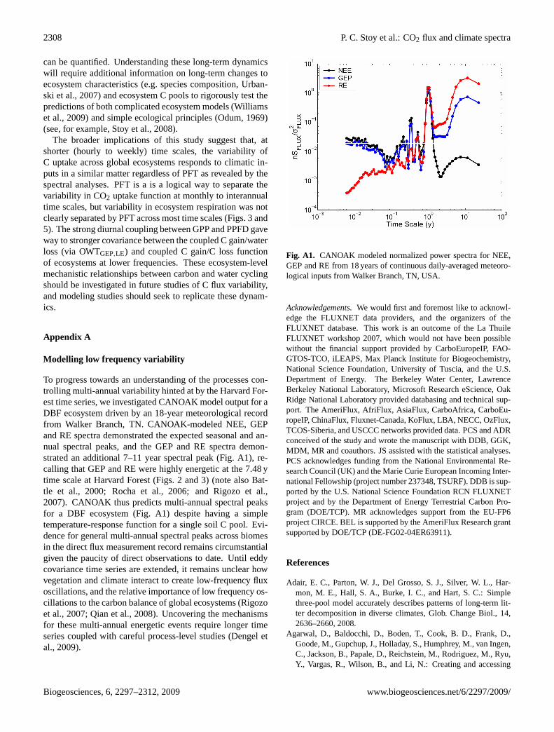
To progress towards an understanding of the processes con-trolling multi-annual variability hinted at by the Harvard For-est time series, we investigated CANOAK model output for aDBF ecosystem driven by an 18-year meteorological recordfrom Walker Branch, TN. CANOAK-modeled NEE, GEPand RE spectra demonstrated the expected seasonal and an-nual spectral peaks, and the GEP and RE spectra demon-strated an additional 7–11 year spectral peak (Fig.A1), re-calling that GEP and RE were highly energetic at the 7.48 ytime scale at Harvard Forest (Figs.2 and3) (note alsoBat-tle et al., 2000; Rocha et al., 2006; and Rigozo et al.,2007). CANOAK thus predicts multi-annual spectral peaksfor a DBF ecosystem (Fig.A1) despite having a simpletemperature-response function for a single soil C pool. Evi-dence for general multi-annual spectral peaks across biomesin the direct flux measurement record remains circumstantialgiven the paucity of direct observations to date. Until eddycovariance time series are extended, it remains unclear howvegetation and climate interact to create low-frequency fluxoscillations, and the relative importance of low frequency os-cillations to the carbon balance of global ecosystems (Rigozoet al., 2007; Qian et al., 2008). Uncovering the mechanismsfor these multi-annual energetic events require longer timeseries coupled with careful process-level studies (Dengel etal., 2009).

Fig. A1. CANOAK modeled normalized power spectra for NEE,GEP and RE from 18 years of continuous daily-averaged meteoro-logical inputs from Walker Branch, TN, USA.

Acknowledgements.We would first and foremost like to acknowl-edge the FLUXNET data providers, and the organizers of theFLUXNET database. This work is an outcome of the La ThuileFLUXNET workshop 2007, which would not have been possiblewithout the financial support provided by CarboEuropeIP, FAO-GTOS-TCO, iLEAPS, Max Planck Institute for Biogeochemistry,National Science Foundation, University of Tuscia, and the U.S.Department of Energy. The Berkeley Water Center, LawrenceBerkeley National Laboratory, Microsoft Research eScience, OakRidge National Laboratory provided databasing and technical sup-port. The AmeriFlux, AfriFlux, AsiaFlux, CarboAfrica, CarboEu-ropeIP, ChinaFlux, Fluxnet-Canada, KoFlux, LBA, NECC, OzFlux,TCOS-Siberia, and USCCC networks provided data. PCS and ADRconceived of the study and wrote the manuscript with DDB, GGK,MDM, MR and coauthors. JS assisted with the statistical analyses.PCS acknowledges funding from the National Environmental Re-search Council (UK) and the Marie Curie European Incoming Inter-national Fellowship (project number 237348, TSURF). DDB is sup-ported by the U.S. National Science Foundation RCN FLUXNETproject and by the Department of Energy Terrestrial Carbon Pro-gram (DOE/TCP). MR acknowledges support from the EU-FP6project CIRCE. BEL is supported by the AmeriFlux Research grantsupported by DOE/TCP (DE-FG02-04ER63911).

References

Adair, E. C., Parton, W. J., Del Grosso, S. J., Silver, W. L., Har-mon, M. E., Hall, S. A., Burke, I. C., and Hart, S. C.: Simplethree-pool model accurately describes patterns of long-term lit-ter decomposition in diverse climates, Glob. Change Biol., 14,2636–2660, 2008.

Agarwal, D., Baldocchi, D., Boden, T., Cook, B. D., Frank, D.,Goode, M., Gupchup, J., Holladay, S., Humphrey, M., van Ingen,C., Jackson, B., Papale, D., Reichstein, M., Rodriguez, M., Ryu,Y., Vargas, R., Wilson, B., and Li, N.: Creating and accessing



the global fluxnet data set, Eos Trans. AGU, 88, Abstract B33E-1657, 2007.

Allen, M. R. and Smith, L. A.: Monte Carlo SSA: detecting irreg-ular oscillations in the presence of colored noise, J. Climate, 9,3373–3404, 1996.

Arnone, J. A. I., Verburg, P. S. J., Johnson, D. W., Larsen, J. D., Ja-soni, R. L., Luccesi, A. J., Batts, C. M., von Nagy, C., Coulombe,W. G., Schorran, D. E., Buck, P. E., Braswell, B. H., Coleman,J. S., Sherry, R. A., Wallace, L. L., Luo, Y., and Schimel, D. S.:Prolonged supression of ecosystem carbon dioxide uptake afteran anomalously warm year, Nature, 455, 383–386, 2008.

Aubinet, M., Grelle, A., Ibrom, A., Rannik,U., Moncrieff, J., Fo-ken, T., Kowalski, A. S., Martin, P. H., Berbigier, P., Bernhofer,C., Clement, R., Elbers, J., Granier, A., Grunwald, T., Morgen-stern, K., Pilegaard, K., Rebmann, C., Snijders, W., Valentini,R., and Vesala, T.: Estimates of the annual net carbon and waterexchange of forests: The EUROFLUX methodology, Adv. Ecol.Res., 30, 113–175, 2000.

Baldocchi, D., Falge, E., Gu, L. H., Olson, R., Hollinger, D.,Running, S., Anthoni, P., Bernhofer, C., Davis, K., Evans, R.,Fuentes, J., Goldstein, A., Katul, G., Law, B., Lee, X. H., Malhi,Y., Meyers, T., Munger, W., Oechel, W., U, K. T. P., Pilegaard,K., Schmid, H. P., Valentini, R., Verma, S., Vesala, T., Wilson,K., and Wofsy, S.: FLUXNET: A new tool to study the tem-poral and spatial variability of ecosystem-scale carbon dioxide,water vapor, and energy flux densities, B. Am. Meteorol. Soc.,82, 2415–2434, 2001a.

Baldocchi, D., Falge, E., and Wilson, K.: A spectral analysis ofbiosphere-atmosphere trace gas flux densities and meteorologi-cal variables across hour to multi-year time scales, Agr. ForestMeteorol., 107, 1–27, 2001b.

Baldocchi, D. D. and Wilson, K. B.: Modeling CO2 and water va-por exchange of a temperate broadleaved forest across hourly todecadal time scales, Ecol. Model., 142, 155–184, 2001.

Baldocchi, D. D.: “Breathing” of the terrestrial biosphere: lessonslearned from a global network of carbon dioxide flux measure-ments systems, Turner Review, Aust. J. Bot., 56, 1–26, 2008.

Barbour, M. M., Hunt, J. E., Dungan, R. J., Turnbull, M. H., Brails-ford, G. W., Farquhar, G. D., and Whitehead, D.: Variation in thedegree of coupling betweenδ13C of phloem sap and ecosystemrespiration in two mature Nothofagus forests, New Phytol., 166,497–512, 2005.

Battle, M., Bender, M. L., Tans, P. P., White, J. W. C., Ellis, J. T.,Conway, T., and Francey, R. J.: Global carbon sinks and theirvariability inferred from atmospheric O2 and13C, Science, 287,2467–2470, 2000.

Braswell, B. H., Sacks, W. J., Linder, E., and Schimel, D. S.: Esti-mating diurnal to annual ecosystem parameters by synthesis of acarbon flux model with eddy covariance net ecosystem exchangeobservations, Glob. Change Biol., 11, 335–355, 2005.

Canadell, J. G., Le Quere, C., Raupach, M. R., Field, C. B., Buiten-huis, E. T., Ciais, P., Conway, T. J., Gillett, N. P., Houghton, R.A., and Marland, G.: Contributions to accelerating atmosphericCO2 growth from economic activity, carbon intensity, and effi-ciency of natural sinks, P. Natl. Acad. Sci. USA, 104, 18353–18354, 2007.

Carvalhais, N., Reichstein, M., Seixas, J., Collatz, G. J., Pereira, J.S., Berbigier, P ., Carrara, A., Granier, A., Montagnani, L., Pa-pale, D., Rambal, S., Sanz, M. J., and Valentini, R.: Implications

of the carbon cycle steady state assumption for biogeochemicalmodeling performance and inverse parameter retrieval, GlobalBiogeochem. Cy., 22, GB2007, doi:10.1029/2007GB003033,2008.

Cava, D., Giostra, U., Siqueira, M. B. S., and Katul, G. G.: Orga-nized motion and radiative perturbations in the nocturnal canopysublayer above an even-aged pine forest, Bound.-Lay. Meteorol.,112, 129–157, 2004.

Chapin III, F. S., Sturm, M., Serreze, M. C., McFadden, J. P., Key,J. R., Lloyd, A. H., McGuire, A. D., Rupp, T. S., Lynch, A.H., Schimel, J. P., Beringer, J., Chapman, W. L., Epstein, H. E.,Euskirchen, E. S., Hinzman, L. D., Jia, G., Ping, C.-L., Tape, K.D., Thompson, C. D. C., Walker, D. A., and Welker, J. M.: Roleof land-surface changes in arctic summer warming, Science, 310,657–660, 2005.

Ciais, P., Reichstein, M., Viovy, N., Granier, A., Ogee, J., Allard, V.,Aubinet, M., Buchmann, N., Bernhofer, C., Carrara, A., Cheval-lier, F., de Noblet, N., Friend, A. D., Friedlingstein, P., Grunwald,T., Heinesch, B., Keronen, P., Knohl, A., Krinner, G., Lousteau,D., Manca, G., Matteucci, G., Miglietta, F., Ourcival, J. M., Pa-pale, D., Pilegaard, K., Rambal, S., Seufert, G., Soussana, J. F.,Sanz, M. J., Schulze, E. D., Vesala, T., and Valentini, R.: Europe-wide reduction in primary productivity caused by the heat anddrought in 2003, Nature, 437, 529–533, 2005.

Cook, B. D., Holladay, S., Santhana-Vannan, S. K., Pan, J. Y., Jack-son, B., and Wilson, B.: FLUXNET: Data from a global networkof eddy-covariance flux towers, Eos Trans. AGU, 88, Fall Meet.Suppl., Abstract B33E–1656, 2007.

Curiel Yuste, J., Janssens, I. A., Carrara, A., and Ceulemans, R.:Annual Q10 of soil respiration reflects plant phenological pat-terns as well as temperature sensitivity, Glob. Change Biol., 10,161–169, 2004.

Daly, E., and Porporato, A.: A review of soil moisture dynamics:from rainfall infiltration to ecosystem response, Environ. Eng.Sci., 22, 9–24, 2005.

Daubechies, I.: Ten lectures on wavelets, SIAM: Society for Indus-trial and Applied Mathematics, 377 pp., 1992.

Davidson, E. A., and Janssens, I. A.: Temperature sensitivity of soilcarbon decomposition and feedbacks to climate change, Nature,440, 165–173, 2006.

Delpierre, N., Soudani, K., Francois, C., Kostner, B., Pontailler,J.-Y., Nikinmaa, E., Misson, L., Aubinet, M., Bernhofer, C.,Granier, A., T., G., Heinesch, B., Longdoz, B., Ourcival, J.-M.,Rambal, S., Vesala, T., and E., D.: Exceptional carbon uptake ineuropean forests during the warm spring of 2007: a data-modelanalysis, Glob. Change Biol., 15, 1455–1474, 2009.

Dengel S., Aeby, D., Grace, J.: A relationship between galacticcosmic radiation and tree rings, New Phytol., 184, 545–551,doi:10.1111/j.1469-8137.2009.03026.x, 2009.

Drake, J., Stoy, P. C., Jackson, R. B., and DeLucia, E. H: Fine rootrespiration in a loblolly pine (Pinus taeda) forest: Proximal lim-its, temperature dependence, and dynamic coupling with canopyphotosynthesis, Plant Cell Environ., 31, 1663–1672, 2008.

Dunn, D. C. and Morrison, J. F.: Analysis of the energy budget inturbulent channel flow using orthogonal wavelets, Comput. Flu-ids, 34, 199–224, 2005.

Ellsworth, D. S.: CO2 enrichment in a maturing pine forest: areCO2 exchange and water status in the canopy affected?, PlantCell Environ., 22, 461–472, 1999.



Falge, E., Baldocchi, D., Olson, R., Anthoni, P., Aubinet, M., Bern-hofer, C., Burba, G., Ceulemans, R., Clement, R., Dolman, H.,Granier, A., Gross, P., Grunwald, T., Hollinger, D., Jensen, N.O., Katul, G., Keronen, P., Kowalski, A., Lai, C. T., Law, B. E.,Meyers, T., Moncrieff, J., Moors, E., Munger, J. W., Pilegaard,K., Rannik,U., Rebmann, C., Suyker, A., Tenhunen, J., Tu, K.,Verma, S., Vesala, T., Wilson, K., and Wofsy, S.: Gap fillingstrategies for defensible annual sums of net ecosystem exchange,Agr. Forest Meteorol., 107, 43–69, 2001.

Fraedrich, K. and Larnder, C.: Scaling regimes of composite rainfalltime series, Tellus A, 45, 289–298, 1993.

Frich, P., Alexander, L. V., Della-Marta, P., Gleason, B., Haylock,M., Klein Tank, A. M. G., and Peterson, T.: Observed coherentchanges in climatic extremes during the second half of the twen-tieth century, Clim. Res., 19, 193–212, 2002.

Friedlingstein, P., Cox, P., Betts, R. A., Bopp, L., von Blow, W.,Brovkin, V., Cadule, P., Doney, S. C., Eby, M., Fung, I. Y., Bala,G., John, J., Jones, C. D., Joos, F., Kato, T., Kawamiya, M.,Knorr, W., Lindsay, K., Matthews, H. D., Raddatz, T., Rayner, P.J., Reick, C., Roeckner, E., Schnitzler, K.-G., Schnur, R., Strass-mann, K., Weaver, A. J., Yoshikawa, C., and Zeng, N.: Climate-carbon cycle feedback analysis: results from the C4MIP modelintercomparison, J. Climate, 19, 3337–3353, 2006.

Gilman, D. L., Fuglister, F. J., and Mitchell Jr., J. M.: On the powerspectrum of “red noise”, J. Atmos. Sci., 20, 182–184, 1963.

Granier, A., Reichstein, M., Breda, N., Janssens, I. A., Falge, E.,Ciais, P., Grunwald, T., Aubinet, M., Berbigier, P., Buchmann,N., Facini, O., Grassi, G., Heinesch, B., Ilvesniemi, H., Keronen,P., Knohl, A., Kostner, B., Lagergren, F., Lindroth, A., Longdoz,B., Loustau, D., Mateus, J., Montagnani, L., Nys, C., Moors, E.,Papale, D., Peiffer, M., Pilegaard, K., Pita, G., Pumpanen, J.,Rambal, S., Rebmann, C., Rodrigues, A., Seufert, G., Tenhunen,J., Vesala, T., and Wang, Q.: Evidence for soil water controlon carbon dynamics in European forests during the extremly dryyear: 2003, Agr. Forest Meteorol., 143, 123–145, 2007.

Granier, A., Breda, N., Longdoz, B., Gross, P., and Ngao, J.:Ten years of fluxes and stand growth in a young beech for-est at Hesse, North-eastern France, Ann. Forest Sci., 65, 704,doi:10.1051/forest:2008052, 2008.

Grinsted, A., Moore, J. C., and Jevrejeva, S.: Application of thecross wavelet transform and wavelet coherence to geophysicaltime series, Nonlin. Processes Geophys., 11, 561–566, 2004,http://www.nonlin-processes-geophys.net/11/561/2004/.

Grunwald, T. and Bernhofer, C.: A decade of carbon, water andenergy flux measurements of an old spruce forest at the AnchorStation Tharandt, Tellus B, 59, 387–396, 2007.

Hanson, P. J., Amthor, J. S., Wullschleger, S. D., Wilson, K. F.,Grant, R. F., Hartley, A., Hui, D. F., Hunt, E. R. J., Johnson,D. W., Kimball, J. S., King, A. W., Y., L., McNulty, S. G.,Sun, G., Thornton, P. E., Wang, S., Williams, M., Baldocchi,D. D., and Cushman, R. M.: Oak forest carbon and water sim-ulations: model intercomparisons and evaluations against inde-pendent data., Ecol. Monogr., 74, 443–489, 2004.

Hibbard, K., Law, B. E., Reichstein, M., Sulzman, J., Aubinet, M.,Baldocchi, D., Bernhofer, C., Bolstad, P., Bosc, A., Campbell, J.,Cheng, Y., Curiel Yuste, J., Curtis, P., Davidson, E. A., Epron,D., Granier, A., Grnwald, T., Hollinger, D., Janssens, I., Long-doz, B., Loustau, D., Martin, J., Monson, R., Oechel, W., Pippen,J., Ryel, R., Savage, K., Scott-Denton, L., Subke, J.-A., Tang, J.,

Tenhunen, J., Turcu, V., and Vogel, C. S.: An analysis of soil res-piration across northern hemisphere temperate ecosystems, Bio-geochemistry, 73, 29–70, 2005.

Hogberg, P., Nordgren, A., Buchmann, N., Taylor, A. F. S., Ekblad,A., Hogberg, M. N., Nyberg, G., Ottoson-Lofvenius, M., andRead, D. J.: Large-scale forest girdling shows that current pho-tosynthesis drives soil respiration, Nature, 411, 789–792, 2001.

Houghton, R. A.: Interannual variability in the global carbon cycle,J. Geophys. Res.-Atmos., 105, 20121–20130, 2000.

Irvine, J., Law, B. E., Martin, J., and Vickers, D.: Interannual varia-tion in soil CO2 efflux and the response of root respiration to cli-mate and canopy gas exchange in mature ponderosa pine, Glob.Change Biol., 14, 2848–2859, 2008.

Janssens, I. A., Lankreijer, H., Matteucci, G., Kowalski, A. S.,Buchmann, N., Epron, D., Pilegaard, K., Kutsch, W., Long-doz, B., Grunwald, T., Montagnani, L., Dore, S., Rebmann, C.,Moors, E. J., Grelle, A., Rannik,U., Morgenstern, K., Oltchev,S., Clement, R., Gudmundsson, J., Minerbi, S., Berbigier, P.,Ibrom, A., Moncrieff, J., Aubinet, M., Bernhofer, C., Jensen, N.O., Vesala, T., Granier, A., Schulze, E. D., Lindroth, A., Dolman,A. J., Jarvis, P. G., Ceulemans, R., and Valentini, R.: Productiv-ity overshadows temperature in determining soil and ecosystemrespiration across European forests, Glob. Change Biol., 7, 269–278, 2001.

Jarvis P. G.: The interpretation of the variations in leaf water po-tential and stomatal conductance found in canopies in the field,Philos. T. Roy. Soc. London B., 273, 593–610, 1976.

Juang, J.-Y., Katul, G. G., Siqueira, M. B. S., Stoy, P. C., and Mc-Carthy, H. R.: Investigating a hierarchy of eulerian closure mod-els for scalar transfer inside forested canopies, Bound.-Lay. Me-teorol., 128, 1–32, 2008.

Jung, M., Verstraete, M., Gobron, M., Reichstein, M., Papale, D.,Bondeau, A., Robustelli, M., and Pinty, B.: Diagnostic assess-ment of European gross primary production, Glob. Change Biol.,14, 2349–2364, 2008.

Kato, T. and Tang, Y.: Spatial variability and major controlling fac-tors of CO2 sink strength in Asian terrestrial ecosystems: evi-dence from eddy covariance data, Glob. Change Biol., 14, 2333–2348, 2008.

Katul, G., Leuning, R., and Oren, R.: Relationship between planthydraulic and biochemical properties derived from a steady-statecoupled water and carbon transport model, Plant Cell Environ.,26, 339–350, 2003.

Katul, G. G. and Parlange, M. B.: On the active role of temperaturein surface layer turbulence, J. Atmos. Sci., 51, 2181–2195, 1994.

Katul, G. G. and Parlange, M. B.: Analysis of land surface heatfluxes using the orthonormal wavelet approach, Water Resour.Res., 31, 2743–2749, 1995.

Katul, G. G., Lai, C.-T., Schfer, K. V. R., Vidakovic, B., Albertson,J. D., Ellsworth, D. S., and Oren, R.: Multiscale analysis of vege-tation surface fluxes: from seconds to years, Adv. Water Resour.,24, 1119–1132, 2001.

Katul, G. G., Porporato, A., Daly, E., Oishi, A. C., Kim, H.-S.,Stoy, P. C., Juang, J.-Y., and Siqueira, M. B. S.: On the spec-trum of soil moisture in a shallow-rooted uniform pine forest:from hourly to inter-annual time scales, Water Resour. Res., 43,W05428, doi:10.1029/2006WR005356, 2007.

Lasslop, G., Reichstein, M., Papale, D., Richardson, A. D., Arneth,A., Barr, A. G., Stoy, P. C., and Wohlfahrt, G.: Separation of


http://www.nonlin-processes-geophys.net/11/561/2004/


net ecosystem exchange into assimilation and respiration using alight response curve approach: critical issues and global evalua-tion Glob. Change Biol., doi:10.1111/j.1365-2486.2009.02041.x,in press, 2009.

Law, B. E., Falge, E., Gu, L., Baldocchi, D. D., Bakwin, P.,Berbigier, P., Davis, K., Dolman, A. J., Falk, M., Fuentes, J. D.,Goldstein, A., Granier, A., Grelle, A., Hollinger, D., Janssens, I.A., Jarvis, P., Jensen, N. O., Katul, G., Mahli, Y., Matteucci, G.,Meyers, T., Monson, R., Munger, W., Oechel, W., Olson, R., Pi-legaard, K., Paw U, K. T., Thorgeirsson, H., Valentini, R., Verma,S., Vesala, T., Wilson, K., and Wofsy, S.: Environmental controlsover carbon dioxide and water vapor exchange of terrestrial veg-etation, Agr. Forest Meteorol., 113, 97–120, 2002.

Lloyd, J. and Taylor, J. A.: On the temperature dependence of soilrespiration, Funct. Ecol., 8, 315–323, 1994.

Luyssaert, S., Schulze, E.-D., Borner, A., Knohl, A., Hessenmoller,D., Law, B.E., Ciais, P., and Grace, J.: Old-growth forests asglobal carbon sinks, Nature, 411, 213–215, 2008.

Mahecha, M. D., Reichstein, M., Lange, H., Carvalhais, N., Bern-hofer, C., Grunwald, T., Papale, D., and Seufert, G.: Characteriz-ing ecosystem-atmosphere interactions from short to interannualtime scales, Biogeosciences, 4, 743–758, 2007,http://www.biogeosciences.net/4/743/2007/.

Moffat, A. M., Papale, D., Reichstein, M., Hollinger, D. Y.,Richardson, A. D., Barr, A. G., Beckstein, C., Braswell, B. H.,Churkina, G., Desai, A. R., Falge, E., Gove, J. H., Heimann,M., Hui, D., Jarvis, A. J., Kattge, J., Noormets, A., and Stauch,V. J.: Comprehensive comparison of gap-filling techniques foreddy covariance net carbon fluxes, Agr. Forest Meteorol., 147,209–232, 2007.

Odum, E. P.: The strategy of ecosystem development, Science, 164,262–270, 1969.

Oren, R., Hsieh, C. I., Stoy, P. C., Albertson, J. D., McCarthy, H.R., Harrell, P., and Katul, G. G.: Estimating the uncertainty inannual net ecosystem carbon exchange: spatial variation in tur-bulent fluxes and sampling errors in eddy-covariance measure-ments, Glob. Change Biol., 12, 883–896, 2006.

Owen, K. E., Tenhunen, J., Reichstein, M., Wang, Q., Falge, E.,Geyer, R., Xiao, X., Stoy, P., Ammann, C., Arain, A., Aubi-net, M., Aurela, M., Bernhofer, C., Chojnicki, B., Granier, A.,Grunwald, T., Hadley, J., Heinesch, B., Hollinger, D., Knohl,A., Kutsch, W., Lohila, A., Meyers, T., Moors, E., Moureaux,C., Pilegaard, K., Saigusa, N., Verma, S., Vesala, T., and Vogel,C.: Linking flux network measurements to continental scale sim-ulations: ecosystem CO2 exchange capacity under non-water-stressed conditions, Glob. Change Biol., 13, 734–760, 2007.

Palmroth, S., Maier, C. A., McCarthy, H. R., Oishi, A. C., Kim,H.-S., Johnsen, K. H., Katul, G. G., and Oren, R.: Contrastingresponses to drought of the forest floor CO2 efflux in a loblollypine plantation and a nearby oak-hickory forest, Glob. ChangeBiol., 11, 421–434, 2005.

Papale, D., Reichstein, M., Aubinet, M., Canfora, E., Bernhofer, C.,Kutsch, W., Longdoz, B., Rambal, S., Valentini, R., Vesala, T.,and Yakir, D.: Towards a standardized processing of Net Ecosys-tem Exchange measured with eddy covariance technique: algo-rithms and uncertainty estimation, Biogeosciences, 3, 571–583,2006,http://www.biogeosciences.net/3/571/2006/.

Parton, W. J., Schimel, D. S., Cole, C. V., and Ojima, D. S.: Anal-

ysis of factors controlling soil organic levels of grasslands in theGreat Plains, Soil Sci. Soc. Am. J., 51, 1173–1179, 1987.

Peters, O., Hertlein, C., and Christensen, K.: A complexity view ofrainfall, Phys. Rev. Lett., 88, 018701–018704, 2002.

Porporato, A., D’Odorico, P., Laio, F., Ridolfi, L., and Rodriguez-Iturbe, I.: Ecohydrology of water-controlled ecosystems, Adv.Water Resour., 25, 1335–1348, 2002.

Potter, C. S., Klooster, S. A., Steinbach, M., Tan, P., Kumar, V.,Shekhar, S., Nemani, R., and Myneni, R. B.: Global telecon-nections of climate to terrestrial carbon flux, J Geophys. Res.,108(D17), 4556, doi:10.1029/2002JD002979, 2003.

Potter, C. S., Klooster, S. A., Tan, P., Steinbach, M., Kumar, V.,and Genovese, V.: Variability in terrestrial carbon sinks over twodecades: Part 2 - Eurasia, Global Planet. Change, 49, 177–186,2005.

Qian, H., Renu, J., and Zeng, N.: Response of the terrestrial carboncycle to the El Nino-Southern Oscillation, Tellus B, 60, 537–550,2008.

Reichstein, M., Tenhunen, J., Roupsard, O., Ourcival, J.-M., Ram-bal, S., Miglietta, F., Peressotti, A., Pecchiari, M., Tirone, G., andValentini, R.: Inverse modeling of seasonal drought effects oncanopy CO2/H2O exchange in three Mediterranean ecosystems,J Geophys. Res., 108(D23), 4726, doi:10.1029/2003JD003430,2003.

Reichstein, M., Falge, E., Baldocchi, D., Papale, D., Aubinet,M., Berbigier, P., Bernhofer, C., Buchmann, N., Gilmanov, T.G., Granier, A., Grnwald, T., Havrankova, K., Ilvesniemi, H.,Janous, D., Knohl, A., Laurila, T., Lohila, A., Loustau, D., Mat-teucci, G., Meyers, T., Miglietta, F., Ourcival, J.-M., Pumpanen,J., Rambal, S., Rotenberg, E., Sanz, M., Tenhunen, J., Seufert,G., Vaccari, F., Vesala, T., Yakier, D., and Valentini, R.: Onthe separation of net ecosystem exchange into assimilation andecosystem respiration: review and improved algorithm, Glob.Change Biol., 11, 1424–1439, 2005.

Reichstein, M., Ciais, P., Papale, D., Valentini, R., Running, S.,Viovy, N., Cramer, W., Granier, A., Ogee, J., Allard, V., Aubi-net, M., Bernhofer, C., Buchmann, N., Carrara, A., Grunwald,T., Heimann, M., Heinesch, B., Knohl, A., Kutsch, W., Loustau,D., Manca, G., Matteucci, G., Miglietta, F., Ourcival, J. M., Pile-gaard, K., Pumpanen, J., Rambal, S., Schaphoff, S., Seufert, G.,Soussana, J. F., Sanz, M. J., Vesala, T., and Zhao, M.: Reductionof ecosystem productivity and respiration during the Europeansummer 2003 climate anomaly: a joint flux tower, remote sens-ing and modelling analysis, Glob. Change Biol., 13, 634–651,2007a.

Reichstein, M., Papale, D., Valentini, R., Aubinet, M., Bernhofer,C., Knohl, A., Laurila, T., Lindroth, A., Moors, E., Pilegaard,K., and Seufert, G.: Determinants of terrestrial ecosystem car-bon balance inferred from European eddy covariance flux sites,Geophys. Res. Lett., 34, L01402, doi:10.1029/2006GL027780,2007b.

Richardson, A. D., Hollinger, D. Y., Burba, G. G., Davis, K. J.,Flanagan, L. B., Katul, G. G., Munger, J. W., Ricciuto, D. M.,Stoy, P. C., Suyker, A. E., Verma, S. B., and Wofsy, S. C.: Amulti-site analysis of random error in tower-based measurementsof carbon and energy fluxes, Agr. Forest Meteorol., 136, 1–18,2006.

Richardson, A. D., Hollinger, D. Y., Aber, J. D., Ollinger, S. V., andBraswell, B. H.: Environmental variation is directly responsible


http://www.biogeosciences.net/4/743/2007/



for short- but not long-term variation in forest-atmosphere carbonexchange, Glob. Change Biol., 13, 788–803, 2007.

Richardson, A. D., Mahecha, M. D., Falge, E., Kattge, J., Moffat,A. M., Papale, D., Reichstein, M., Stauch, V. J., Braswell, B.H., Churkina, G., Kruijt, B., and Hollinger, D. Y.: Statisticalproperties of random CO2 flux measurement uncertainty inferredfrom model residuals, Agr. Forest Meteorol., 148, 38–50, 2008.

Rigozo, N. R., Nordemann, D. J. R., da Silva, H. E., Echer, M.P. d. S., and Echer, E.: Solar and climate signal records in treering width from Chile (AD 1587–1994), Planet. Space Sci., 55,158–164, 2007.

Rocha, A. V., Goulden, M. L., Dunn, A. L., and Wofsy, S. C.:On linking interannual tree ring variability with observationsof whole-forest CO2 flux, Glob. Change Biol., 12, 1378–1389,2006.

Ryan, M. G. and Law, B. E.: Interpreting, measuring, and modelingsoil respiration, Biogeochemistry, 73, 3–27, 2005.

Saito, M. and Asunama, J.: Eddy covariance calculation revisitedwith wavelet cospectra, Sola, 4, 49–52, 2008.

Scanlon, T. M. and Albertson, J. D.: Turbulent transport of car-bon dioxide and water within vegetation canopies during unsta-ble conditions: identification of episodes using wavelet analysis,J. Geophys. Res.-Atmos., 106, 7251–7262, 2001.

Schar, C., Vidale, P. L., Luthi, D., Frei, C., Haberli, C., and Liniger,M. A.: The role of increasing temperature variability in Europeansummer heatwaves, Nature, 427, 332–336, 2004.

Scheffer, M., Carpenter, S. R., Foley, J. A., Folke, C., and Walker,B. H.: Catastrophic shifts in ecosystems, Nature, 413 591–596,2001.

Siqueira, M. B. S., Katul, G. G., Sampson, D. A., Stoy, P. C.,Juang, J.-Y., McCarthy, H. R., and Oren, R.: Multi-scale modelinter-comparisons of CO2 and H2O exchange rates in a matur-ing southeastern U.S. pine forest, Glob. Change Biol., 12, 1189–1207, 2006.

Stoy, P. C., Katul, G. G., Siqueira, M. B. S., Juang, J.-Y., McCarthy,H. R., Kim, H.-S., Oishi, A. C., and Oren, R.: Variability innet ecosystem exchange from hourly to inter-annual time scalesat adjacent pine and hardwood forests: a wavelet analysis, TreePhysiol., 25, 887–902, 2005.

Stoy, P. C., Palmroth, S., Oishi, A. C., Siqueira, M. B. S., Juang,J.-Y., Novick, K. A., Ward, E. J., Katul, G. G., and Oren, R.:Are ecosystem carbon inputs and outputs coupled at short timescales? A case study from adjacent pine and hardwood forestsusing impulse-response analysis, Plant Cell Environ., 30, 700–710, 2007.

Stoy, P. C., Katul, G. G., Siqueira, M. B. S., Juang, J.-Y., Novick,K., McCarthy, H. R., Oishi, A. C., and Oren, R.: Role of vege-tation in determining carbon sequestration along ecological suc-cession in the southeastern United States, Global Change Biol.,14, 1409–1427, 2008.

Taneva, L., Pippen, J. S., Schlesinger, W. H., and Gonzalez-Meler,M. A.: The turnover of carbon pools contributing to soil CO2 andsoil respiration in a temperate forest exposed to elevated CO2concentration, Glob. Change Biol., 12, 983–994, 2006.

Tang, J., Baldocchi, D., and Xu, L.: Tree photosynthesis modulatessoil respiration on a diurnal time scale, Glob. Change Biol., 11,1298–1304, 2005.

Thomas, C. K., Law, B. E., Irvine, J., Martin, J. G., Pettijohn,J. C., and Davis, K. J.: Seasonal hydrology explains inter-annual and seasonal variation in carbon and water exchange ina semi-arid mature Ponderosa Pine forest in Central Oregon, J.Geophys. Res.- Biogeosciences, doi:10.1029/2009JG001010, inpress, 2009.

Torrence, C. and Compo, G. P.: A practical guide to wavelet analy-sis, B. Am. Meteorol. Soc., 79, 61–78, 1998.

Urbanski, S. P., Barford, C., Wofsy, S., Kucharik, C. J., Pyle, E. H.,Budney, J., McKain, K., Fitzjarrald, D., Czikowsky, M. J., andMunger, J. W.: Factors controlling CO2 exchange on timescalesfrom hourly to decadal at Harvard Forest, J. Geophys. Res., 112,G02020, doi:10.1029/2006JG000293, 2007.

Valentini, R., Matteucci, G., Dolman, A. J., Schulze, E. D., Reb-mann, C., Moors, E. J., Granier, A., Gross, P., Jensen, N. O.,Pilegaard, K., Lindroth, A., Grelle, A., Bernhofer, C., Grunwald,T., Aubinet, M., Ceulemans, R., Kowalski, A. S., Vesala, T., Ran-nik, U., Berbigier, P., Loustau, D., Guomundsson, J., Thorgeirs-son, H., Ibrom, A., Morgenstern, K., Clement, R., Moncrieff, J.,Montagnani, L., Minerbi, S., and Jarvis, P. G.: Respiration as themain determinant of carbon balance in European forests, Nature,404, 861–865, 2000.

Vickers, D., Thomas, C. K., Martin, J. G., and Law, B. E.: Self-correlation between assimilation and respiration resulting fromflux partitioning of eddy-covariance CO2 fluxes, Agr. Forest Me-teorol., 149, 1552–1555, 2009.

Williams, M., Richardson, A. D., Reichstein, M., Stoy, P. C.,Peylin, P., Verbeeck, H., Carvalhais, N., Jung, M., Hollinger, D.Y., Kattge, J., Leuning, R., Luo, Y., Tomelleri, E., Trudinger,C. M., and Wang, Y.-P.: Improving land surface models withFLUXNET data, Biogeosciences, 6, 1341–1359, 2009,http://www.biogeosciences.net/6/1341/2009/.

Wilson, K. B., Baldocchi, D. D., and Hanson, P. J.: Leaf age affectsthe seasonal pattern of photosynthetic capacity and net ecosys-tem exchange of carbon in a deciduous forest, Plant Cell Envi-ron., 24, 571–583, 2001.



Documents

Biosphere-atmosphere exchange of CO2 in relation to climate: a