The CSIRO Atmosphere Biosphere Land Exchange

The CSIRO Atmosphere Biosphere Land Exchange (CABLE) model for use in climate models and as an offline model E. A. Kowalczyk, Y. P. Wang, R. M. Law, H. L. Davies, J. L. McGregor and G. Abramowitz CSIRO Marine and Atmospheric Research paper 013 November 2006

The CSIRO Atmosphere Biosphere Land Exchange (CABLE) model for use in climate models and as an offline model E. A. Kowalczyk, Y. P. Wang, R. M. Law, H. L. Davies, J. L. McGregor and G. Abramowitz CSIRO Marine and Atmospheric Research paper 013 November 2006

Abstract Over the past twenty years, land surface models have developed from simple schemes to more complex representations of soil-vegetation-atmosphere interactions, allowing for linkages between terrestrial microclimate, plant physiology and hydrology. This evolution has been facilitated by advances in plant physiology and the availability of global fields of land surface parameters obtained from remote sensing. The CSIRO Atmosphere Biosphere Land Exchange (CABLE) model presented here calculates carbon, water and heat exchanges between the land surface and atmosphere and is suitable for use in climate models and in the form of a one-dimensional stand-alone model. We provide a full description of CABLE and examples of offline and online simulations for selected sites. Online simulations are performed with CABLE coupled to the CSIRO Conformal-Cubic Atmospheric Model (C-CAM). The model version presented here represents the first phase of a longer-term plan to improve the land surface schemes in the CSIRO and the Australian Community Earth System Simulator (ACCESS) global circulation models. This report is intended for users and future developers of CABLE.

National Library of Australia Cataloguing-in-Publication

The CSIRO Atmosphere Biosphere Land Exchange (CABLE) model for use in climate models and as an offline model.

Bibliography. ISBN 1 921232 39 0 (pdf.). 1. Biogeochemical cycles - Mathematical models. 2. Biosphere - Mathematical models. I. Kowalczyk, E. A. (Eva A.). II. CSIRO. Marine and Atmospheric Research. (Series : CSIRO Marine and Atmospheric Research paper ; 13). 577.14

Enquiries should be addressed to: E. A. Kowalczyk CSIRO Marine and Atmospheric Research PMB 1, Aspendale, Victoria 3195, Australia Phone: +61 3 9239 4524 Fax: +61 3 9239 4444 Email: [email protected] Important Notice © Copyright Commonwealth Scientific and Industrial Research Organisation (‘CSIRO’) Australia 2006 All rights are reserved and no part of this publication covered by copyright may be reproduced or copied in any form or by any means except with the written permission of CSIRO. The results and analyses contained in this Report are based on a number of technical, circumstantial or otherwise specified assumptions and parameters. The user must make its own assessment of the suitability for its use of the information or material contained in or generated from the Report. To the extent permitted by law, CSIRO excludes all liability to any party for expenses, losses, damages and costs arising directly or indirectly from using this Report. Use of this Report The use of this Report is subject to the terms on which it was prepared by CSIRO. In particular, the Report may only be used for the following purposes. � this Report may be copied for distribution within the Client’s organisation; � the information in this Report may be used by the entity for which it was prepared (“the Client”), or by the Client’s contractors and agents, for the Client’s internal business operations (but not licensing to third parties); � extracts of the Report distributed for these purposes must clearly note that the extract is part of a larger Report prepared by CSIRO for the Client. The Report must not be used as a means of endorsement without the prior written consent of CSIRO. The name, trade mark or logo of CSIRO must not be used without the prior written consent of CSIRO.

Contents

1 Introduction 1

2 Model history 1

3 Model description 2

3.1 Basic formulations for land surface processes. . . . . . . . . . . . . . . . . . . 3

3.1.1 Model structure . . . . . . . . . . . . . . . . . . . . . . . . . . . . . 4

3.1.2 Formulation of aerodynamic resistances. . . . . . . . . . . . . . . . . 6

3.2 Canopy model . . . . . . . . . . . . . . . . . . . . . . . . . . . . . . . . . . . 8

3.2.1 Radiation transfer in plant canopies . . . . . . . . . . . . . . . . . . . 8

3.2.2 The coupled model of stomatal conductance, photosynthesis and parti-tioning of net available energy . . . . . . . . . . . . . . . . . . . . . . 12

3.2.3 An iterative method for the solution of the coupled canopy model equa-tions. . . . . . . . . . . . . . . . . . . . . . . . . . . . . . . . . . . . 14

3.2.4 Description of the photosynthesis model . . . . . . . . . . . . . . . . . 16

3.3 Soil model . . . . . . . . . . . . . . . . . . . . . . . . . . . . . . . . . . . . 19

3.3.1 Soil Surface Energy Balance and Fluxes . . . . . . . . . . . . . . . . 19

3.3.2 Soil moisture . . . . . . . . . . . . . . . . . . . . . . . . . . . . . . . 20

3.3.3 Solution of soil moisture equation . . . . . . . . . . . . . . . . . . . . 21

3.3.4 Soil temperature . . . . . . . . . . . . . . . . . . . . . . . . . . . . . 24

4 Model simulations 25

4.1 Climate-carbon feedback simulations. . . . . . . . . . . . . . . . . . . . . . . 32

5 Final comments 35

6 Acknowledgments 35

CSIRO Atmosphere Biosphere Land Exchange model for use in climate models 1

1 Introduction

Atmospheric general circulation models (GCM) require a description of radiation, heat, wa-ter vapour and momentum fluxes across the land-surface atmosphere interface. Land surfaceschemes (LSS) are designed to calculate the temporal evolution of these fluxes, differentiatingbetween bare ground and vegetation fluxes. The presence of vegetation affects climate by mod-ifying the energy, momentum, and water balance of the land surface and changing atmosphericCO2 concentrations. Associated with the effect of vegetation on climate, is the question of howthe climate change may affect plant physiological properties and thus productivity. Increasingpublic interest in climate change has led to the need to develop more complete models of the cli-mate system including the incorporation of the carbon cycle. In a coupled climate-carbon cyclemodel, plants affect climate and CO2 concentrations while climate affects physiological param-eters and productivity of plants. The CSIRO Atmosphere Biosphere Land Exchange (CABLE)LSS incorporates biogeochemical knowledge and is coupled with the CSIRO global ConformalCubic Atmospheric Model (C-CAM) and elements of the terrestrial carbon cycle.

The biosphere atmosphere exchange model described in this technical paper represents Phase1 of a long-term plan to improve the representation of surface processes in the CSIRO andACCESS GCMs. The main purpose of the present technical paper is to provide a detaileddescription of CABLE.

2 Model history

The CSIRO land surface scheme has evolved from a simple scheme to a complex representationof biosphere atmosphere interaction. The main CSIRO GCM in 1990 had a single soil type,constant roughness length over land and no allowance for vegetation. It used the soil-moisturescheme of Deardorff [1977] and the force-restore method of Deardorff [1978] to calculate sur-face temperature. In 1991, a simple stand alone model of soil/canopy based on a big leaf descrip-tion of a canopy and a force-restore model for soil was formulated by Kowalczyk et al. [1991].The model was then implemented into the CSIRO GCM in 1993 as described in Kowalczyk et al.[1994]. The new scheme included a number of new features such as soil type (hence variablethermal and moisture properties), albedo, roughness length, canopy resistance, canopy intercep-tion of rainfall, runoff, deep soil percolation, snow accumulation and melting. The canopy wasrepresented as a single vegetation layer with the characteristics of a large leaf acting as a sourceor sink of water vapour and sensible heat. The canopy temperature was calculated from thesolution of the surface energy balance equation while the stomatal resistance was a function ofradiation, saturation deficit, temperature and water stress.

In 1995 an improved version of soil/snow model was implemented into the CSIRO GCM and theCSIRO regional model, DARLAM (Division of Atmospheric Research Limited Area Model).The emphasis in the model development was to improve the seasonal simulation of soil moisture,heat cycles and snow cover. The multilayer soil model computed soil temperature and moisturedifferentiating between liquid water and ice content of the soil, whereas the new snow modelwas expanded to compute the temperature, snow density and thickness of three snowpack layersand a physically based snow albedo.

In 1997 the Raupach et al. [1997] Soil Canopy Atmosphere Model (SCAM) was developed asan offline version. SCAM included a canopy layer above the soil surface; formulation of anaerodynamic conductance for the turbulent transfer between soil, vegetation and atmosphere(accounting for turbulent exchanges within canopies) and responses of canopy stomata to radia-tion, saturation deficit, temperature and water stress. In 1998, SCAM was coupled to DARLAM


and was used to simulate energy fluxes measured during the CSIRO field program OASIS (Ob-servations at Several Interacting Scales) as described in Finkele et al. [2003].

In 1998, a one layer two-leaf canopy model was formulated by Wang and Leuning [1998] onthe basis of a multilayer model of Leuning et al. [1995]. A comparison of both one layer andmultilayer model results showed consistency in the predictions of fluxes over a range of leafarea index values. Since the one layer model was ten times computationally more efficient thanthe multilayer model, it was more suitable for use in global circulation models. The one layermodel differentiates between sunlit and shaded leaves, hence two sets of physical and physi-ological parameters were devised to represent the bulk properties of sunlit and shaded leaves.Several improvements were made to the one layer model, namely: allowance for non-sphericalleaf distribution, an improved description of the exchange of solar and thermal radiation, andmodification of the stomatal model of Leuning et al. [1995] to include the effects of soil waterdeficit on photosynthesis and respiration. The model was further refined by Wang [2000]. In2003 the first version of CABLE which included the two-leaf canopy model, the canopy tur-bulence model and the multilayer soil/snow model was coupled with C-CAM. The subsequentaddition of a simple carbon pool model to C-CAM, facilitated the completion of the Phase 1C4MIP (Coupled Carbon Cycle Climate Model Intercomparison Project) experiment which re-quired simulation of the twentieth century climate.

3 Model description

CABLE is a model of biosphere atmosphere exchange allowing for interaction between micro-climate, plant physiology and hydrology.

The main features of CABLE are:

1. The vegetation is placed above the ground allowing for full aerodynamic and radiativeinteraction between vegetation and the ground.

2. A coupled model of stomatal conductance, photosynthesis and partitioning of absorbednet radiation into latent and sensible heat fluxes.

3. The model differentiates between sunlit and shaded leaves i.e. two-big-leaf submodel forcalculation of photosynthesis, stomatal conductance and leaf temperature.

4. The radiation submodel calculates the photosynthetically active radiation (PAR), near in-frared and thermal radiation.

5. The plant turbulence model by Raupach et al. [1997] is used to calculate air temperatureand humidity within the canopy.

6. Annual plant net primary productivity is determined from the annual carbon assimilationcorrected for respiratory losses. The seasonal growth/decay of biomass is determined bypartitioning of the assimilation product between leaves, roots and wood. The flow ofcarbon between the vegetation and soil is described at present by a simple carbon poolmodel [Dickinson et al., 1998].

7. A multilayer soil model is used. The Richards’ equation is solved for soil moisture whilethe heat conduction equation is used for soil temperature.

8. The snow model computes the temperature, density and thickness of three snowpack lay-ers.


CABLE consists of a number of submodels: (a) canopy processes, (b) soil and snow, (c) carbonpool dynamics and soil respiration.

3.1 Basic formulations for land surface processes.

CABLE calculates the temporal evolution of CO2, radiation, heat, water and momentum fluxesat the surface. The vertical eddy fluxes of heat, water and momentum are dependent on themean properties of the flow through the use of aerodynamic resistances. The general form forthe sensible and latent heat fluxes is

H�ρa cp � w � T � �� u � T� �� Tsur � Tref � � rH (1)

E�ρa � w � q � � � u � q � �� qsur � qref � � rE � (2)

Tref and qref are air temperature and specific humidity at the reference level, and Tsur and qsurare surface values, ρa is air density, cp is the specific heat, u � ,T� , q � are turbulent scales forvelocity, temperature and humidity, rH is aerodynamic resistance for heat and rE the resistancefor water exchange between the surface and a reference level, w � T � is the turbulent heat fluxand w � q � is the turbulent moisture flux. rE comprises aerodynamic as well as plant stomatalresistance. Knowledge of surface temperature Tsur is required for the computation of fluxes. Tsuris obtained through the closure of the energy balance at the lower atmosphere boundary whichis one of the main tasks of the land surface scheme. The energy balance equation is solved forthe temperature of the surface which may consist of a combination of surface elements such asvegetation, bare ground, snow and ice. The energy balance for any particular surface is writtenhere as:

Rn � G � H � λE (3)

where Rn is the net radiation flux at the surface, G is the thermal storage flux (negligible forvegetation), with the sum of the latent (λE) and the sensible (H) heat fluxes defining the availableenergy. In CABLE the vegetation is placed above the ground allowing for full aerodynamic andradiative interaction between the vegetation and the ground. Hence the total surface fluxes forthe combined canopy ground system are the sum of the fluxes from the soil (s) to the canopy airspace and the fluxes from the canopy (c) to the atmosphere:

HT � Hs � Hc (4)λET � λEs � λEc � (5)

Central to the calculation of surface fluxes is the parameterization of aerodynamic resistanceswhich depends on the reference level for the atmospheric variables T and q and the descriptionof canopy aerodynamics. Raupach et al. [1997] developed a sophisticated description of single-layer canopy aerodynamics, including treatment of canopy turbulence (see section 3.1.2). Heused Monin and Obukhov [1954] similarity theory for the parameterization of the surface fluxesfor a combined canopy ground system. In the Monin-Obukhov theory the lowest model levellies in the surface layer within which the surface fluxes are constant in the vertical. Integrating


the flux-profile relationship between the roughness length, z0, and the height of the first modellevel, z, results the following relationship [Louis, 1979]:

u � z � � u �k

�ln � z � z0 � � ψM � z � LMO � � ψM � z0

�LMO ��

hence the expression for the friction velocity can be written as:

u � � kUref

ln � zref�z0 � � ψM � ξ � � ψM � ξ z0

�zref � (6)

where zref is the first model level (reference level), Uref is the mean wind at the reference level,k is the von Karman constant (0.4), ψM is Businger-Dyer functions for the flux-profile rela-tionships for momentum for both stable and unstable conditions, LMO is the Monin-Obukhovstability height, and ξ is a nondimensional height.

In order to calculate the friction velocity the nondimensional height ξ, which is a thermal stabil-ity parameter, must be computed:

ξ � zref

LMO(7)

where LMO is defined as [Garratt, 1992]:

LMO � � u3� � � k � g � T � w � T � � � � u3� � � k g HT� � T ρa cp � � (8)

where k is the von Karman constant, g is the gravity constant and w � T � the turbulent heat flux.Substituting Eq. 8 to Eq. 7 and adding a fraction of the latent heat flux (Raupach et al. [1997]Sec. 3.9) gives us the formula for the stability parameter used in CABLE:

ξ � � zref k g � HT � 0 � 07 λET � � � Tref ρa cp u3� � (9)

with HT and λET being total grid fluxes as defined in Eqs. 4 and 5.

The calculation of fluxes, and hence ξ, depends strongly on the surface temperature but simul-taneously the surface temperature depends on ξ, hence, an iteration method is used to allow forsimultaneous calculation of all the required variables using values from the current time step.At the start, neutral stability is assumed so ξ � 0, Tc � Tref and qc � qref. After computation ofthe resistances, fluxes and canopy temperature, a new value of ξ is obtained from Eq. (9). Theiteration is repeated with the new value of ξ. Four iterations are used to obtain final values ofthe stability parameter, surface fluxes and canopy temperature.

3.1.1 Model structure

An iterative procedure, used for the simultaneous calculations of the stability parameter, fluxesand vegetation temperature, imposes a specific model structure where the calculations inde-pendent of the stability parameter are performed outside of the iteration loop. The basic flowdiagram of CABLE is presented in Fig.1, with the stability iteration loop clearly depicted.


Set parameter values and initial states

Main time step loop

Soil and canopy water storage

Initialise radiation

Surface roughness characteristics

Stability iteration loop for

Air properties

Radiation fluxes and surface albedo

Turbulent aerodynamic resistances

Vegetation boundary layer resistances

Leaf temperature iteration loop – calculate fluxes wrt reference level; for sunlit, shaded leaves

Heat conductance

Photosynthesis rates - Rubisco, RuBP and sink limited

Check for convergence

Soil latent, sensible, ground heat fluxes

Solve dispersion matrix for in-canopy temperature, humidity

Recalculate leaf temp and fluxes wrt in-canopy conditions

Latent, sensible fluxes from wet portion of canopy

Canopy sensible, latent heat and canopy net radiation

Stomatal conductance

Dew and canopy storage adjustments for wet canopy fluxes

End time step loop

Call soil carbon and carbon pools routine

Call soil/snow routines

Carbon fluxes

End stability iteration loop

Figure 1: Flow diagram of CABLE.


At the beginning of a time step the following calculations are performed: initialisation of some ofthe radiation terms, evaluation of the canopy and soil water storage from the previous time stepvalues and calculation of surface roughness characteristics. In CABLE the roughness length ofvegetation is a function of canopy height and leaf area index [Raupach, 1994], the latter varyingon a daily basis. The roughness length of the ground is for the transfer from the ground to the in-canopy air space, hence the values are smaller than the typical values used in other land surfaceschemes in which roughness length directly depends on the height of the roughness element.

At each iteration loop, first the fluxes are calculated with reference to (denoted by “wrt” on thediagram) the first model level, then Localised Near Field (LNF) theory [Raupach, 1989a, b] isused for the in-canopy temperature and humidity, before the fluxes are recalculated with refer-ence to the in-canopy variables. A detailed description of the LFN theory application in canopymodelling is given in section 3.3 of Raupach et al. [1997]. All of the variables calculated withinthe stability loop are diagnostic, i.e. they are solutions of various algebraic equations whichare functions of the current step atmospheric forcing, soil heat and water stores. The stabilityiteration loop includes the calculation of:

1. Air properties.

2. Radiation fluxes for canopy and soil, section 3.2.1.

3. Aerodynamic properties, section 3.1.2.

4. Vegetation boundary layer resistances [Leuning et al., 1995] .

5. Solution of the coupled model of stomatal conductance, photosynthesis and partitioningof net available energy, depicted on the diagram as leaf iteration loop, section 3.2.3 .

6. Wet canopy fluxes.

7. Soil latent, sensible and ground heat fluxes, section 3.3.1.

8. Solution of the dispersion matrix [Raupach et al., 1997].

9. Recalculation of fluxes with reference to in-canopy conditions [Raupach et al., 1997].

Following the calculation of the diagnostic variables within the stability loop, the prognosticvariables are solved; the canopy water storage is then adjusted for dew and wet canopy fluxesand the soil model is solved for the current soil moisture and temperature, (see section 3.3).In the presence of snow on the ground, a snow model is used as described in detail in Gordonet al. [2002]. Finally, the carbon routines are called for the calculation of soil respiration andredistribution of the assimilation product between leaves, roots and wood. Soil respiration is asimple function of soil moisture and temperature. The flow of carbon between the vegetationand soil is described at present by a simple carbon pool model [Dickinson et al., 1998]. Thiswill be replaced in the version of CABLE used for ACCESS. The soil respiration formulationwill also change as part of the new carbon pool scheme and hence the current scheme is notdescribed in this report.

3.1.2 Formulation of aerodynamic resistances.

Energy and mass transfer exchange processes between land surfaces and the atmosphere occurover turbulent and laminar pathways. Localised Near Field (LNF) theory is used to describethe turbulent transfer within and above the canopy, see Raupach [1989a], Raupach [1989b].


LNF accounts for the fact that the eddies responsible for most scalar transfer in a canopy havea vertical length scale of the order of a large fraction of the canopy height. In the turbulenttransfer the scalar concentration profile at height z in the air, C � z � , is related to the profiles ofsource strength, S � z � , and bulk vertical flux, F � z � . In LNF, C � z � is comprised from the “far-field”and “near-field” components i.e. C � C f � Cn. Two turbulence properties, vertical velocitystandard deviation σw � z � , and Lagrangian time scale TL � z � are used to describe compliance ofthe “far-field” component with a gradient diffusion relationship between flux and concentration:

F � z � � � K f � z � dC f

dz (10)

K f � z � � σ2w � z � TL � z � (11)

Parameterization of σw � z � is a function of vegetation parameters such as height, h, and leaf areaindex over the whole grid cell, Λ, and the friction velocity, u � (see section 3.5.1):

σw � z � � u � � a23 min � exp � csw Λ � z � h � 1 � � 1 � (12)

where a3 is an aerodynamic parameter which gives the ratio of σw�u � in the inertial sublayer

and csw is a constant describing the rate of decrease of σw with depth.

Parameterization of TL � z � is more complex as it needs to account for different time scales ofturbulence in the layer close to the ground i.e. below the zero-plane displacement d and belowand above the roughness sublayer depth zru f :

TL � z � �� k z

� � a32 u � ψH � ξ � � z � zru f

fsp � Λ � cT L h�u � d � z � zru f

fsp � Λ � cT L h�u � z�d 0 � z � d

(13)

where k is the von Karman constant, ψH is the stability function for scalars,fsp � 1

�max � 23 d

h 1 � is a “sparseness factor” equal to 1 for dense canopy and approaching 0 asΛ � 0, and cTL is a constant (0.4). For detailed discussion on the formulation of TL � z � and σwsee Raupach et al. [1997].

Using σw � z � and TL � z � , an expression for the turbulent aerodynamic resistance from a level zx tothe reference level zref is derived as:

rx �� zref

zx

dzK f � z � �� zref

zx

dzσ2

w � z � TL � z � (14)

Integrating Eq.(14) over selected pathways gives aerodynamic resistances:

rca � � exp � 2cswΛ � 1 � d�h � � � 1 � � � a2

3 fsp � Λ � cTL2cswΛ � d � z � hrcb � dz

� � a23 fsp � Λ � cT L h � h � z � zru f

rcc � 1k

�ln � zref

� � zru f � d � � � ψH � ξ � � ψH � ξ � zru f � d � � zref � � zru f � z � zref

(15)


Total resistance in a single vegetation layer is:

rtc � rca � rcb � rcc (16)

The aerodynamic resistance from the soil to canopy is given by:

rs � lnzref

z0

exp � 2cswΛ � � exp � 2cswΛ � 1 � d�h � �

a23 fsp � Λ � cTL 2cswΛ

(17)

Integrated stability functions, used to calculate aerodynamic canopy resistances and for the cal-culation of the friction velocity, use the Businger-Dyer form for unstable cases and the Webbform for stables cases, see Paulson [1970].For scalar:

ψH � ξ � �� 2 ln� 12 � 1 � y � 2 � with y �� 1 � γhξ � 1 � 4 unstable

� β ξ stable(18)

For momentum:

ψM � ξ � �� ln� 14 � 1 � x � 2 1

2 � 1 � x2 � � � 2arctanx � π2 with x � � 1 � γmξ � 1 � 4 unstable

� β ξ stable(19)

and β � 5 and γm � γh � 16.

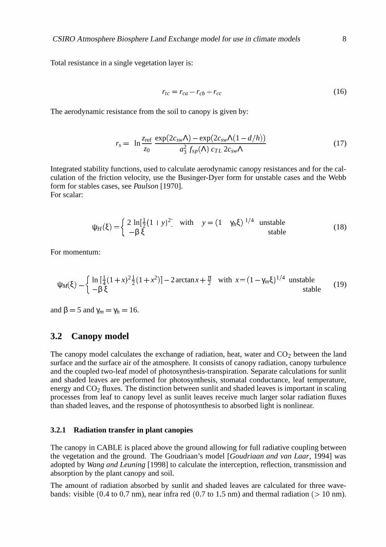
3.2 Canopy model

The canopy model calculates the exchange of radiation, heat, water and CO2 between the landsurface and the surface air of the atmosphere. It consists of canopy radiation, canopy turbulenceand the coupled two-leaf model of photosynthesis-transpiration. Separate calculations for sunlitand shaded leaves are performed for photosynthesis, stomatal conductance, leaf temperature,energy and CO2 fluxes. The distinction between sunlit and shaded leaves is important in scalingprocesses from leaf to canopy level as sunlit leaves receive much larger solar radiation fluxesthan shaded leaves, and the response of photosynthesis to absorbed light is nonlinear.

3.2.1 Radiation transfer in plant canopies

The canopy in CABLE is placed above the ground allowing for full radiative coupling betweenthe vegetation and the ground. The Goudriaan’s model [Goudriaan and van Laar, 1994] wasadopted by Wang and Leuning [1998] to calculate the interception, reflection, transmission andabsorption by the plant canopy and soil.

The amount of radiation absorbed by sunlit and shaded leaves are calculated for three wave-bands: visible � 0 � 4 to 0 � 7 nm), near infra red � 0 � 7 to 1 � 5 nm) and thermal radiation �� 10 nm).


The incoming short-wave radiation from the sun (S0) is the sum of direct beam � Sb � j � and diffuse� Sd � j � radiation. That is:

S0 � ∑j � 1 � 2� Sb � j � Sd � j � (20)

where Sb � j and Sd � j represent the incident direct beam and diffuse radiation in the visible wave� j � 1 � and near infra red � j � 2 � waveband.

The total flux density of radiation within waveband j absorbed by the two big canopy leaves iscalculated as

Q1 � j �� Λ

0q1 � j � λ � fsun � λ � dλ big sunlit leaf (21)

Q2 � j � � Λ

0q2 � j � λ � � 1 � fsun � λ � � dλ big shaded leaf (22)

where λ � �0 Λ � is the cumulative canopy leaf area index from the canopy top. The fraction

of sunlit leaves within a canopy is calculated as fsun � exp � � kbλ � , where kb is the extinctioncoefficient of direct beam radiation for a canopy with black leaves described by Eq. 26.

The flux density of radiation absorbed by a sunlit � q1 � j � and shaded � q2 � j � leaf for visible (PAR)� j � 1 � or near infra red � j � 2 � (NIR) radiation in a canopy is calculated as:

q2 � j � λ � � � 1 � ρtd � j � k �d � j exp � � kd � jλ � Sd � j � � � 1 � ρtb � j � k�b � j exp � � k

�b � jλ � � (23)

� 1 � ω j � kb exp � � kbλ � � Sb � j q1 � j � λ � � q2 � j � λ � � kb � 1 � ω j � Sb � j (24)

where ρtb � j and ρtd � j are the surface (canopy and soil) reflectance for direct beam � b � and diffuseradiation � d � in waveband j, and k �b � j and k �d � j are the extinction coefficients (of direct beam anddiffuse radiation in waveband j) in a real canopy, kd and kb are the extinction coefficients in acanopy with black leaves, and ω j is the scattering coefficient of the leaf in waveband j. Theextinction coefficients and surface reflectances are calculated according to Goudriaan and vanLaar [1994]. k �b � j and k �d � j are related to the extinctions for a canopy with black leaves in thefollowing way:

k�b � j � kb � 1 � ω j � 1

2 and k�d � j � kd � 1 � ω j � 1

2 (25)

and

kb � θ � � Gcos � θ � (26)

kd � � 1Λ

ln� � Λ

0exp � � kb � θ � λ � dλ � (27)


where G is the ratio of the projected area of leaves in the direction perpendicular to the directionof incident solar radiation and the actual leaf area. As an approximation, G can be calculated as

G � φ1 � φ2 cos � θ � (28)φ1 � 0 � 5 � 0 � 633χ (29)

φ2 � 0 � 877 � 1 � 2φ1 �

where χ is an empirical parameter related to the leaf angle distribution and χ � 0 for sphericalleaf angle distribution. The mean inclination angle decreases with an increase in χ. The aboveapproximation for G is applicable for χ within the range of [-0.4,0.6].

The effective canopy-soil reflectance is given by:

ρtb � j � ρcb � j � � ρs � j � ρcb � j � exp � � 2k�b � jΛ � (30)

ρtd � j � ρcd � j � � ρs � j � ρcd � j � exp � � 2k�d � jΛ � (31)

(32)

where ρs � j is soil reflectance in waveband j, ρcb � j and ρcd � j are the reflectances of the canopy fordirect beam and for diffuse radiation, respectively, at the top of the canopy, and are calculatedas:

ρcb � j � 2kb

kb � kdρch � j (33)

ρcd � j � 2 � π � 20

ρcb � j sin � θ � cos � θ � dθ (34)

where ρch � j is the reflectance of a horizontally homogeneous canopy with black horizontalleaves, θ is the zenith angle of the sun.

The surface albedo for shortwave radiation for land is calculated as

αland � 0 � 5 ∑j � 1 � 2� ρtb � j fb � ρtd � j � 1 � fb � � (35)

where fb is the fraction of direct beam incoming short-wave radiation. If fb, is not providedby the atmospheric radiation model, we use the empirical relationships developed by Spitters[1986] to estimate fb. They are:

fb �

��

� 0 0 � 22 � b1

6 � 4 � b1 � 0 � 22 � 2 0 � 22 � b1 � 0 � 35min � 1 � 66b1 � 0 � 4728 1 � b1 � 0 � 35max � 1 � b2 0 � b1 � b2

(36)


and

b1 � S0

Sc � 1 � 0 � 033cos � 2π � Dy � 10 � � 365 � � cos � θ � (37)

b2 �� 1 � 47 � b3 � � 1 � 66 (38)b3 � 0 � 847 � cosθ � 1 � 04cos � θ � � 1 � 61 � (39)

where Sc is a solar constant (Sc � 1370Wm� 2) and Dy is a day of year.

The net long wave radiation balance of a leaf depends on leaf temperature which is calculated bysolving the combined equations for leaf energy partitioning and photosynthesis (section 3.2.2).However, the solutions to the combined equations require the input of the net available energy,Rni, which includes the net long wave radiation. To overcome this difficulty, we calculate thenet long wave radiation absorbed by the leaf under isothermal conditions (i.e. where leaf tem-perature Tf � i is equal to air temperature Ta), and describe the difference in the absorbed longwave radiation between isothermal and non-isothermal conditions using radiative conductance(section 3.2.2).

The upwards and downwards long wave radiation flux densities within the canopy under isother-mal conditions are calculated as:

L� � λ � �� 1 � exp � � kd � Λ � λ � � � L f � exp � � kd � Λ � λ � � Ls (40)

L � � λ � �� 1 � exp � � kdλ � � L f � exp � � kdλ � La (41)

where La, L f and Ls are the long wave radiation flux densities from sky, leaf under isothermalcondition and soil, respectively, and are calculated from the Stefan-Boltzmann law:

La � εaσT 4a L f � ε f σT 4

f Ls � εsσT 4s � (42)

where εa, ε f and εs are the emissivities and Ta, Tf and Ts are the temperatures of the sky, leafand soil, respectively. The absorbed thermal radiation (wave band j � 3) flux density by a leaf inthe canopy (qi � 3) is then given by

qi � 3 � d � L � � L � �dλ � kd exp � � kd � Λ � λ � � � Ls � L f � � kd exp � � kdλ � � La � L f � (43)

The total flux density of absorbed long wave radiation by all sunlit leaves � Q1 � 3 � and shaded� Q2 � 3 � leaves are then given by

Q1 � 3 �� Λ

0fsun � λ � qi � 3 � λ � dλ �� Ls � L f � kd

�exp � � kdΛ � � exp � � kbΛ � � � � kd � kb � (44)

� kd � La � L f � � 1 � exp � � � kb � kd � Λ � � � kd � kb �Q2 � 3 �� Λ

0� 1 � fsun � λ � � qi � 3 � λ � dλ �� 1 � exp � � kdΛ � � � Ls � La � 2L f � � Q1 � 3 (45)

The net available energy for the big leaf i under isothermal conditions is calculated as


Rnc � i �3

∑j � 1

Qi � j i � 1 2 (46)

3.2.2 The coupled model of stomatal conductance, photosynthesis and partitioning of netavailable energy

CABLE calculates photosynthesis, transpiration and sensible heat fluxes, separately for sunlitand shaded leaves. The distinction between sunlit and shaded leaves is necessary in scalingfrom leaf to canopy as the response of photosynthesis to the absorbed photosynthetically activeradiation (PAR) is nonlinear.

Wang and Leuning [1998] compared the bulk formulation for the two leaf model with a multi-layered canopy model and found that the simulated fluxes of CO2, water and sensible heat bythe two leaf model agreed very closely with those from the multi-layered canopy model. Thetwo-leaf model uses the same set of equations for calculating photosynthesis, transpiration andsensible heat fluxes for an individual leaf, but with the bulk formulation for the parameters for allsunlit and shaded leaves separately. For a given leaf parameter P, the corresponding parametervalues for the two big leaves are calculated as

P1 � � Λ

0p � λ � fsun � λ � dλ big sunlit leaf (47)

P2 �� Λ

0p � λ � � 1 � fsun � λ � � dλ big shaded leaf

The basic set of equations for the coupled model of stomatal conductance, photosynthesis andtranspiration for the big sunlit and shaded leaves is:

energy balance

Rnc � i � λEc � i � Hc � i (48)

latent heat flux

λEc � i � sRnc � i � cpρaDa � Gh � i � Gr� i �s � γ � Gh � i � Gr� i � � Gw� i

(49)

sensible heat flux

Hc � i � Gh � icpρa � Tf � i � Ta � (50)

stomatal conductance

Gst � i � G0 � i

bsc� a fwAc � i

Cs � i � 1 � Ds � i�Ds0 � (51)


photosynthesis-gas diffusion

Ac � i � bscGst � i � Cs � i � Ci � � Gc � i � Ca � Ci � (52)

and photosynthesis-biochemistry

Ac � i � Vn � i � Rd � i (53)

where

� Rnc � i is the net available energy partitioned into latent, λEc � i, and sensible, Hc � i, heat fluxes,

� Da, Ta and Ca are vapour pressure deficit, temperature and CO2 within the canopy space,respectively,

� Eq. 49 is a Penman-Monteith combination equation for latent heat flux, s is the slope ofthe curve relating saturation water vapour to temperature, and γ is psychrometric constant,

� in the Ball-Berry-Leuning model for stomatal conductance (Eq. 51), G0 � i is stomatal con-ductance of a leaf for H2O when net leaf photosynthesis is zero, Ds � i is vapour pressuredeficit at the leaf surface, fw is an empirical parameter describing the availability of soilwater for plants, and a and Ds0 are empirical constants (the equation is applicable to C3and C4 plants with different values of a, Ds0 and G0 � i),

� in Eq. 52 describing supply of CO2 by diffusion through stomata and the leaf boundarylayers, Ac � i is the net photosynthesis rate, Cs � i is the CO2 concentration at the leaf surfaceand Ci is intercellular CO2 concentration of the leaf,

� in the biochemical demand equation (53), the net photosynthesis rate is calculated as thedifference between net carboxylation rate of the big leaf Vn � i and day respiration rate Rd � i.Carboxylation is the chemical reaction that reduces CO2 into carbonic acid. The reactioncan be limited in two ways, by the availability of substrate, ribulose-1, 5-bisphosphate(RuBP-limited), or by the availability of the Rubisco enzyme, ribulose-1, 5-bisphosphatecarboxylase-oxygenase, (Rubisco-limited),

� conductances Gw � i, Gh � i and Gr� i are for water, heat and radiation respectively, Gb � i isboundary layer conductance and Gc � i is total conductance for CO2 from the intercellu-lar space to the reference height; they are calculated as:

water G� 1w� i � G

� 1a � i � G

� 1b � i � G

� 1st � i (54)

heat G� 1h � i � G

� 1a � i � � nbbhGb � i � � 1 (55)

boundary layer Gb � i � Gbu � i � Gb f � i (56)

radiation Gr� i � 4 ε f σbT 3a�cp (57)

total G� 1c � i � G

� 1a � i � � bbcGb � i � � 1 � � bscGst � i � � 1 (58)


where bbc � 1 � 27, bsc � 1 � 57, bbh � 1 � 075, and n=1 for amphistomatous leaves, and n=2for hypostomatous ones. For a description of the calculation of boundary layer conduc-tance Gb � i see Wang and Leuning [1998]. The aerodynamic Ga � i conductance is givenby:

Ga � i � u � � rtc

where rtc is described by Eq. 16. Gr� i is the radiative conductance, see Wang and Leuning[1998].

3.2.3 An iterative method for the solution of the coupled canopy model equations.

The set of equations 48 to 53 has 6 unknowns; T f � i, Ds � i, Cs � i, Ci, Ac � i, and Gst � i which need to becalculated to obtain the photosynthesis (Ac � i), transpiration (λEc � i) and sensible heat flux (Hc � i)for a given set of atmospheric forcing and soil moisture conditions. Analytical solutions do notexist for all of the equations so an iterative method is required.

At the beginning of each time step we calculate aerodynamic and boundary layer resistances andthe radiation absorbed by the canopy for the given meteorological forcing. As leaf temperature,Tf � i, is required for the calculation of the absorbed radiation energy, we approximate Rnc � i usingthe isothermal net radiation as described in Sec. 3.2.1:

Rnc � i � R�n � i � cp Gr� i � Tf � i � Ta � (59)

where the last term describes the loss of thermal radiation of the big leaf under non-isothermalconditions. For the purpose of iteration we write the equations for the coupled model in thefollowing way:

Gst � i � G0 � i

bsc� a fwAc � i

Cs � i � 1 � Ds � i�Ds0 � (60)

Ac � i � bscGst � i � Cs � i � Ci � � Gc � i � Ca � Ci � (61)Ac � i � min � VJ � i Vc � i Vp � i � � Rd � i (62)

λEc � i � sRnc � i � cpρaDa � Gh � i � Gr� i �s � γ � Gh � i � Gr� i � � Gw � i

(63)

R�n � i � cp Gr� i∆Ti � λEc i � Hc � i � λEc i � cpρaGh � i∆Ti (64)

Ds � iGst � i �� Da � s∆Ti � Gw� i (65)

where ∆Ti � Tf � i � Ta.

At the first iteration we set the leaf temperature to the air temperature at the reference level i.e.Tf � i � Ta � Tref and hence ∆Ti � 0. Cs � i and Ds � i are set to the reference height values above thecanopy i.e. Ca and Da. The iteration method is as follows:

1. Eqs. 60 to 62 provide a description of photosynthesis. Given values of ∆Ti, Cs � i, andDs � i the equations can be solved analytically (see section 3.2.4) for the remaining threeunknowns Ci, Ac � i and Gst � i.


� the analytical solution for Ci requires evaluation of the photosynthetic parameters Vx(maximum rate of Rubisco-limited carboxylation) and Jx (maximum rate of poten-tial electron transport). Both are dependent on leaf temperature T f � i as described inLeuning [2002]. Various other parameters related to photosynthesis and respirationare obtained before the calculation of Ci can be completed, see section 3.2.4.

� the analytic solution for Ci for the RuBP-limited and Rubisco-limited case is de-scribed by:

Ci � � b1 � � b21 � 4b0b2 � 1 � 22b2

(66)

and comes from the solution of the Eq. 89 which in turns come from the simultaneoussolution of Eqs. 60, 61 and 62, as formulated by Leuning [1990]. For the descriptionof bi, where i � 0 1 2 see section 3.2.4.

� the carboxylation rates are evaluated separately for the RuBP-limited VJ � i, Rubisco-limited Vc � i and sink-limited Vp � i cases, see section 3.2.4.

� the net photosynthesis rate is calculated using the equation for biochemical demandfor CO2 (Eq. 62) which requires the minimum of the RuBP-limited, Rubisco-limitedand sink-limited carboxylation rates.

� having generated a new value of the net photosynthesis, we compute the stomatalconductance Gst � i using Eq. 60.

� Eq. 61 is rearranged to give a new value of Cs � i

Cs � i � Ci � � Ca � Ci � Gc � i� � bscGst � i � (67)

This completes the computation of the photosynthesis variables Ac � i, Gst � i, Ci andCs � i.

2. Having computed Gst � i, the total conductance for water, Gw� i, is obtained from Eq. 54.

3. Penman-Monteith combination equation 63 is used for the canopy transpiration (λEc � i).

4. Sensible heat flux is calculated using Eq. 64.

5. Eq. 50 is now used to obtain a new value of leaf temperature T f � i.

6. Eq. 65 gives a new value of Ds � i.

This completes the iteration for the 6 unknowns and evaluation of the fluxes of photosynthesis,transpiration and sensible heat. The new values of ∆Ti, Cs � i and Ds � i can now be used in the nextiteration. The iteration is repeated until,

abs � ∆T iter � 1i � ∆T iter

i � � 0 � 01 (68)

see figure 1.


3.2.4 Description of the photosynthesis model

A description of the uptake of CO2 by leaves requires a model for the CO2 supply by diffusionfrom the ambient air to intercellular spaces and the demand for CO2 by biochemical reactionsof photosynthesis, Eq. 62. The net carboxylation rate in Eq. 62 is given by:

Vn � i � min � VJ � i Vc � i Vp � i � (69)

where VJ � i, Vc � i and Vp � i are the RuBP-limited, Rubisco-limited and sink-limited carboxylationrates. C3 and C4 plants have different photosynthetic pathways. Hence we present a descriptionfor each type before a mixed C3

�C4 model is described.

a) C3 plants

For C3 plants, the RuBP-limited photosynthetic rate, V3J � i, is calculated as

V3J � i � Ji

4Ci � Γ �

Ci � 2Γ � (70)

where Γ � is the CO2 compensation point in the absence of day respiration � R3d � i � 0 � , Ji isthe electron transport rate and is given by the smaller positive root of the following quadraticequation:

γ3J2i � � α3Q3i � 1 � J3x � i � Ji � α3Q3i � 1J3x � i � 0 (71)

where γ3 is an empirical parameter varying from 0 to 1, α3 is the quantum efficiency of RuBPproduction and J3x � i is the maximum rate of potential electron transport (Eqs. 100 and 101) ofthe big leaf i at leaf temperature Tf � i. Q3i � 1 is the absorbed PAR (see Eqs. 21 and 22) � Q3i � 1 �� 1 � c4 � Qi � 1 � and c4 is a fraction of C4 plants in the grid.

The Rubisco-limited photosynthetic rate for C3 plants, V3c � i is calculated as

V3c � i � V3x � i � Ci � Γ � �Ci � Kc � 1 � O

�K0 � (72)

where Kc and K0 are the Michaelis-Menten constants for RuBP carboxylation and RuBP oxy-genation respectively, O is the intercellular oxygen concentration and V3x � i is the maximum car-boxylation rate (Eqs. 98 and 99) of leaf i at leaf temperature T f � i.

The sink-limited photosynthetic rate, V3p � i for C3 plants is calculated as

V3p � i � 0 � 5V3x � i � (73)

Day respiration rate is calculated as

R3d � i � 0 � 015V3x � i (74)


Respiration by leaves is included within the photosynthesis calculation while respiration bywoody tissue and roots is dependent on temperature and the relevant carbon pool size. Detailsof the temperature dependence are given in Wang et al. [2006].

b) C4 plants

RuBP-limited V4J � i is given by the smaller positive root of the following quadratic equation:

γ4V 24J � i � � α4Q4i � 1 � V4x � i � V4 � i � α4Q4i � 1V4x � i � 0 (75)

where γ4 is an empirical constant, α4 is the quantum efficiency of C4 photosynthesis, Q4i � 1 is theabsorbed PAR (Q4i � 1 � c4Qi � 1 � , and V4x � i is the maximum carboxylation rate (Eqs. 102 and 103)of the big C4 leaf.

The Rubisco-limited (V4c � i) photosynthetic rate is calculated as

V4c � i � V4x � i � (76)

The sink-limited carboxylation rate is calculated as:

V4p � i � b4V4x � iCi (77)

where b4 is an empirical constant.

The day respiration rate of big leaf i is

R4d � i � 0 � 025V4x � i (78)

c) mixed C3/C4 model

Instead of applying the photosynthesis model for C3 and C4 plants separately we use the follow-ing formulation to calculate photosynthesis for a C3/C4 mixed grid cell (the formulation is alsoapplicable to pure C3 or C4 grid cells).

When photosynthesis is either limited by Rubisco carboxylase or RuBP regeneration, Eq. 62 canbe written in a more general form as

Ac � i � Ci � Γ �Ci � Cx � i

V3 � i � Ri � (79)

Note that subscripts J and c were dropped in V3 � i as it represents both. For Rubisco carboxylase-limited photosynthesis rate, V3 � i, Cx � i and Ri are given by

V3 � i � V4x � i (80)Cx � i � Kc � 1 � O

�K0 � (81)

Ri � R3d � i � R4d � i � V4x � i � (82)


K0, and Kc are functions of leaf temperature. For RuBP-limited photosynthesis rate, V3 � i, Cx andR are given by

V3 � i � Ji

4 (83)

Cx � i � 2Γ � (84)Ri � R3d � i � R4d � i � V4J � i � (85)

Γ � , K0 is a function of leaf temperature. Eq. 60 for stomatal conductance can be written for aC3/C4 mixed grid cell as

Gst � i � G0c � XAc � i (86)

where

G0c �� 1 � c4 � G03 � c4G04 (87)

X � � 1 � c4 � a3 fw

� Cs � i � Γ � � 1 � Ds � i�D3 � �

c4a4 fw

� Cs � i � Γ � � 1 � Ds � i�D4 � (88)

where X is the so called Leuning constant. Eqs. 61, 79 and 86 can be solved analytically forAc � i, Ci and Gst � i for given values of Cs � i, Ds � i and leaf temperature (Tf � i) [Leuning, 1990]. Theanalytic solution for Ci is given by the larger, positive root (Eq. 66) of the following equation:

b2C2i � b1Ci � b0 � 0 (89)

where

b2 � G0c � X � V3 � i � Ri � (90)b1 �� 1 � XCs � i � � V3 � i � Ri � � G0c � Cx � i � Cs � i � � X � V3 � iΓ

� � Cx � iRi � (91)b0 �� 1 � XCs � i � � V3 � iΓ

� � Cs � iRi � � G0cCx � iCs � i (92)

When photosynthesis is sink-limited, the carboxylation rate Vp � i is calculated as:

Vp � i � 0 � 5V3x � i � b4V4x � iCi (93)

The above equation can be combined with Eq. 61 and 86 to solve for Ac � i, Ci and Gst � i, and Ac � iis the smaller positive root of the following equation:

b5A2c � i � b6Ac � i � b7 � 0 � (94)


where

b5 � X (95)b6 � G0c � b4V4x � i � 1 � XCs � i � � X � Rd � 0 � 5V3x � i � (96)

b7 � G0c � b4Cs � iV4x � i � 0 � 5V3x � i � Rd � (97)

The maximum carboxylation rate V3x � i and maximum rate of potential electron transport J3x � i forC3 plants are calculated as:

V3x � 1 �� 1 � c4 � vc max � 25 fvc max 3 � Tf � 1 � � Λ

0exp � � kbλ � exp � � knλ � dλ (98)


0� 1 � exp � � kbλ � � exp � � knλ � dλ (99)

J3x � 1 �� 1 � c4 � jmax � 25 f j max 3 � Tf � 1 � � Λ

0exp � � kbλ � exp � � knλ � dλ (100)

J3x � 2 �� 1 � c4 � jmax � 25 f j max 3 � Tf � 2 � � Λ

0� 1 � exp � � kbλ � � exp � � knλ � dλ (101)

The maximum carboxylation rate of C4 plants, V4x � i is calculated as:


0exp � � kbλ � exp � � knλ � dλ (102)


0� 1 � exp � � kbλ � � exp � � knλ � dλ (103)

where fvc max 3 � Tf � i), fvc max 4 � Tf � i), describe the temperature dependence of vc max � 25 for C3 andC4 plants. f j max 3 � Tf � i) describes the temperature dependence of maximum potential electrontransport rate of C3 plants. vc max � 25 and jmax � 25 are the maximum carboxylation rate and maxi-mum potential electron transport rate respectively for a leaf i. We assume jmax � 25 � 2vc max � 25.

3.3 Soil model

In order to simulate climate in GCMs, a realistic representation of soil temperature and moistureavailability as well as their long term evolution is required. The soil model presented here hassix layers and three prognostic variables namely, soil temperature, liquid water, and ice content.The amount of ice formed or melted is calculated from energy and mass conservation.

3.3.1 Soil Surface Energy Balance and Fluxes

Soil latent and sensible heat fluxes are obtained from the bulk transfer relations:

Hs � ρcp � Ts � Tref � � rs (104)λEsp � λρ � q � � Ts � � qref � � rs (105)


where Ts is the soil surface temperature and rs the resistance given by equation (17). Esp is apotential evaporation which is the maximum possible evaporation from a surface under givenatmospheric conditions and unlimited soil water supply. The Penman-Monteith combinationequation [Garratt, 1992], provides an alternative formulation for the potential soil evaporationin the model. In this approach the combination of the energy and the aerodynamic contributionto evaporation is used as described by the first and second term, respectively:

λEsl � Γ � RNs � Gs � � � 1 � Γ � ρλδqd�rs (106)

where Γ � s� � s � γ � , s is ∂q � � ∂T , γ � cp

�λ the psychrometric constant, and δqd is the humidity

deficit in the air. RNs is the net radiative flux to the soil surface, and Gs is the heat flux into thesoil.

For a wet surface Esl � Esp while for a dry surface Esl � Esp, see [Kowalczyk et al., 1991]. Theactual evaporation from the soil surface is set to a fraction, x, of the potential evaporation Esp orEsl:

λEs � xλEsp or λEs � xλEsl (107)

To calculate Hs and Es, knowledge of soil surface temperature and moisture is required; we usevalues obtained at the previous timestep. The determination of the current time step surfacetemperature is based on the surface energy balance, which can be described as:

RNs � Gs � Hs � λEs (108)

The net radiation at the soil surface comprises a combination of shortwave and longwave fluxessuch that

RNs � � 1 � αs � S � � L � � εsL�

(109)

where S � is the incoming shortwave radiation, L � is the downward longwave flux and L� � σT 4

sis the upward longwave flux at the soil surface, αs is the albedo and εs is emissivity of the surface.Flux Gs is given to the soil temperature diffusion equation (eq. 126) as the upper boundarycondition (see section 3.3.4).

3.3.2 Soil moisture

The soil is a heterogeneous system composed of three constituent phases, namely the solid phase,water, and air [Hillel, 1982]. Water and air compete for the same pore space and continuallychange their volume fractions due to precipitation, evapotranspiration, snow melt and drainage.Soil hydraulic and thermal characteristics depend on the soil type as well as frozen and unfrozensoil moisture content. In this model, soil moisture is assumed to be at ground temperature, sothere is no heat exchange between the moisture and the soil due to the vertical movement ofwater. Volumetric soil moisture, η, is considered in terms of liquid and ice components, η �ηl � ηi. Ice decreases soil porosity but liquid moisture can move through remaining unfrozen soil


pores. Each soil type is described by the following hydraulic characteristics: saturation contentηsat , wilting content ηw, and field capacity η f c. ηsat is equal to the volume of all the soil poreswhich can fill with water under extremely wet conditions. Here, an additional variable, actualsaturation ηAsat is used. Actual saturation excludes the pores filled with ice, ηAsat � ηsat � ηi.

The one-dimensional conservation equation for soil moisture in the absence of ice is describedby

∂η∂t ��

∂F∂z� r � z � (110)

where F is the soil water flux and the r term includes runoff, drainage and root extraction forevapotranspiration. Water flux, F , in an unsaturated soil is given by Darcy’s law

F � K � K∂ψ∂z � K � D

∂η∂z (111)

where K is the hydraulic conductivity, ψ is the matric potential and D � � K∂ψ�∂η

is the diffusivity. Combining Eqs. 110 and 111 we obtain the Richard’s equation

∂η∂t � �

∂∂z � K � D

∂η∂z � � r � z � � (112)

To solve Eq.112 we need to assume forms of the relationship between the hydraulic conductivity,the matric potential, and the soil moisture content. The dependencies of Clapp and Hornberger[1978] are used,

K � Ks � ηl

ηAsat� 2b � 3 ψ � ψs � ηl

ηAsat� � b (113)

where Ks and ψs are the values at saturation and b is a non-dimensional constant. ηAsat iscalculated on the assumption that soil ice becomes part of the solid matrix. If we define thefractional liquid content as a function of actual saturation, ηl f � ηl

�ηAsat and substitute relations

(113) into Eq. (112), we obtain the equation for the liquid water transfer in the soil:

∂ � ηAsat ηl f �∂t � ∂

∂z � Ksψs b ηb � 2l f

∂ηl f

∂z � Ks η2b � 3l f � � r � z � � (114)

3.3.3 Solution of soil moisture equation

We first note that ηAsat may vary from timestep to timestep if the fraction of frozen soil alters.However, for the purposes of solving Richard’s equation, (114), we need to assume that ηAsatremains constant during the timestep, whence a sequential solution in split manner gives thefollowing pair of equations;an advective equation

ηAsat∂ηl f

∂t� ∂

∂z

�Ksη2b � 3

l f � � 0 (115)


and a diffusive equation including the sources and sinks

ηAsat∂ηl f

∂t �∂∂z � Ksψsbηb � 2

l f

∂ηl f

∂z � � r � z � � (116)

The 6 soil layers have mid-layer depths z1 z2 z3 z4 z5 z6; the soil layers lie between the half-level depths z0 � 5 z1 � 5 z2 � 5 z3 � 5 z4 � 5 z5 � 5 z6 � 5 with z defined as positive downwards.

Soil moisture vertical advection

Equation (115) has the nature of an advection equation in terms of ηl f , producing fluxes ofηAsat ηl f , with a downward advective “velocity”, c, given by

c � min�Ksη2b � 2

l f ∆z�∆t � � (117)

The velocities are calculated at the half-level interfaces at the current time τ, using the smallerof the neighbouring values of ηl f in order to avoid potential problems from isolated frozen soillayers, in which case ηl f will be very small. For numerical stability, it is imposed that theCourant number of the velocity is less than 1, which leads to the minimization condition in(117) involving ∆z, the distance between the adjacent “full” levels; in particular for sand, c maybecome rather large due to the relatively large value of Ks= 0.000166 ms

� 1.

Equation (115) is solved by the total variation diminishing (TVD) method. As discussed byDurran [1999], TVD methods avoid the growth of spurious ripples in the solution.

Low- and high-order fluxes are defined at the half-levels as follows. Noting that c is alwayspositive downwards, the low-order flux is the first-order upstream expression

FLk � 1 � 2 � ck � 1 � 2ηl f k (118)

where, ηl f k denotes ηl f with k subscript. The following high-order flux is used, based on theLax-Wendroff method

FHk � 1 � 2 � ck � 1 � 2

2� zk � 1ηl f k � zkηl f k � 1 �

� zk � 1 � zk � �c2

k � 1 � 2∆t

2� ηl f k � 1 � ηl f k �� zk � 1 � zk � � (119)

In the TVD method, these fluxes are combined using a flux-limiter, C, such that the net flux F isgiven by

Fk � 1 � 2 � FLk � 1 � 2 � Ck � 1 � 2 �

FHk � 1 � 2 � FL

k � 1 � 2 � � (120)

We choose to use the “superbee” flux limiter of Roe [1985],

Ck � 1 � 2 � max � 0 min � 1 2sk � 1 � 2 � min � 2 sk � 1 � 2 �� (121)


where

sk � 1 � 2 � � ηl f k � ηl f k � 1

ηl f k � 1 � ηl f k � � (122)

The smoothness variable sk � 1 � 2 represents the ratio of the slope of the solution upstream ofk � 1�2 to the slope of the solution across the interface at k � 1

�2 itself; s is approximately unity

where the numerical solution is smooth [Durran, 1999], in which case the flux will be weightedtowards the higher-order expression; s is negative when there is a local maximum or minimumimmediately upstream of k � 1

�2, in which case Ck � 1 � 2 becomes zero and the low-order flux is

used. The final solution to (115) is given by

η �l f k � ητl f k � ∆t � Fk � 1 � 2 � Fk � 1 � 2

zk � 1 � 2 � zk � 1 � 2 � � ητAsat k (123)

where values at the current time step are denoted by superscript τ and those after this advectivetime step by � . Note that at the top and bottom half-levels, z0 � 5 and z6 � 5, the velocities andadvective fluxes are set to zero.

There is an extra constraint applied to prevent soil layers from exceeding their saturated value.This is achieved by solving (123) from the lowest layer upwards; if for any layer this would leadto it being supersaturated, then the Fk � 1 � 2 flux is reduced accordingly.

Soil moisture vertical diffusion

The diffusion equation 116 is also written in terms of half-level fluxes for ηAsatηl f . It is solvedfor the current time step using as initial conditions η �l f from (123), as produced by the advectionequation. In order to cope with the possibility of large diffusivities, implicit time differencing isused for the diffusion equation, leading to

ητAsat

�ητ � 1

l f � η �l f �∆t � ∂

∂z� Ksψsbηb � 2

l f

∂ητ � 1l f

∂z � � rτ � z � � (124)

The solution of this equation calculates fluxes at the half levels using diffusivities� � Ksψsbηb � 2l f

where the half-level ηl f are linearly averaged from the adjacent full-level values of η �l f . In finitedifference form, (124) is expressed as

ητAsat k ητ � 1

l f k

∆t � 1

� zk � 0 � 5 � zk � 0 � 5 �� ητ � 1l f k � 1 � ητ � 1

l f k

zk � 1 � zk� �� ητ � 1

l f k � ητ � 1l f k � 1

zk � zk � 1 �� ητ

Asat k η �k∆t

� rτk � (125)


This may be readily solved using a tridiagonal solver. The top and bottom boundary conditionof zero diffusive fluxes is achieved by setting

� � � � �� 0 � The top layer includes r1 termsthat represent the flux infiltrating the surface which depends on rainfall, snowmelt, evaporation,surface runoff and soil hydrological properties. At the bottom, non-zero gravitational drainageacts towards restoring the water profile to its field capacity, via the term r6.

3.3.4 Soil temperature

The vertical temperature profile is described by the following equation:

ρscs∂Ts

∂t �∂∂z � κs

∂Ts

∂z � (126)

where ρs is the density � kgm� 3 � , cs is the specific heat (J kg

� 1K� 1) and κs is the thermal

conductivity (W m� 1 K

� 1) of the soil. The volumetric heat capacity (ρs cs) is calculated as theweighted sum of the heat capacity of dry soil, liquid water and ice (air heat capacity is neglected),

ρs cs �� 1 � ηsat � ρdsoil cdsoil � ηl ρw cw � ηi ρice cice � (127)

The soil dry density is estimated using soil porosity and assuming the same unit weight, ρws, forsolid components,

ρsoil �� 1 � ηsat � ρws � (128)

Soil thermal conductivity κs plays a crucial role in determining the depth of freezing/thawing asit varies by about one order of magnitude as the soil approaches saturation point and increasesfurther due to the ice content. A method for predicting κs in both frozen and unfrozen soils isbased on Johansen [1975]. κs, is calculated as a combination of dry, κdry, and saturated, κsat ,conductivities, weighted by a normalized thermal conductivity called the Kersten number,

κs � Kr � κsat � κdry � � κdry � (129)

κdry is a function of the soil dry density. κsat depends on the soil porosity ηsat , the quartz content,and the liquid and ice volume fraction, whilst the Kersten number Kr is a simple function ofsaturation. The presence of water or ice in the soil can alter the soils thermal properties andthus modify soil temperature by several degrees. To take this into consideration the soil thermalproperties are recalculated at each time step.

The bottom boundary condition for Eq. (126) is zero heat flow. At the top boundary the net heatflux at the surface is given by the Gs flux, see Eq. 108.

Following the solution of Eqs. (114) and (126) the freezing/thawing calculations are performed.If a soil layer temperature cools below freezing point and there is still unfrozen soil moisture,ice is formed. The amount of ice formed in a layer of thickness, δz, is limited by the amount ofliquid water and available energy


ρw δzδηi � min�ρw ηl δz � Tf rz � Ts � ρscsδz

L f

� (130)

where L f is the latent heat of fusion and Tf rz is the freezing temperature. During freezing,latent heat is released from the soil and thus the soil is warmed. The layer temperature dropsbelow freezing after all the water in the soil turns into ice. The melting process occurs whenthe temperature of a soil layer with ice increases to 0 � C. The amount of ice melted is calculatedin a similar fashion. In reality, the natural water in the soil and rocks freezes over a range oftemperatures below 0 � C.

4 Model simulations

To illustrate CABLE’s capability in simulating diverse climatic conditions, we present examplesof the model’s simulations at three selected sites covered with vegetation: tropical rainforest,high latitude coniferous forest and Australian eucalyptus forest. The surface parameters for thesites are chosen not from the actual observed site descriptions, but from the C-CAM simulationwith the resolution of 2x2 � . At this resolution the model has only 13 vegetation types and 9 soiltypes with prescribed parameters relevant for each type.

The tropical rainforest site is in the Amazon Basin ( � 4 � 6 � 299 � 5 � ). Figure 2 shows time seriesof various model variables for the period of 15 days in June obtained from the coupled C-CAM/CABLE simulation forced by observed sea surface temperatures. The site is characterisedby the following parameters: leaf area index above 5 (plotted on panel j) as lai/10), tree heightof 35 m and the soil type is clay.

Panel d) shows the partitioning of the available energy for the canopy into latent and sensibleheat fluxes, with the latent heat flux composed of transpiration and wet evaporation (direct evap-oration from the water stores on the canopy). In the Amazon basin, wet evaporation constitutesa significant part of the latent heat flux due to frequent precipitation events as depicted in panele). In June precipitation is frequent but not large, as this is the beginning of the dry season whichcan be observed by the continuous decline in the moisture at all the soil levels, see panel g). Evenwith a decrease in precipitation, the major part of the available radiation is allocated to evapo-transpiration as the tropical forest root system can access the deep soil moisture accumulatedthrough the wet season.

Net radiation for soil is about 20% of that for the canopy due to canopy shading effects, (seepanel f). Small latent heat flux and negligible sensible heat flux are due to the aerodynamicsheltering of the ground by the high forest with large LAI, resulting in most of the available netradiation going into soil ground heat flux. Diurnal amplitude of soil temperature is only up toabout 6 � C, see panel h), and is smaller than the diurnal variation of air temperature depicted onpanel b), due to shading and radiation effects of vegetation.

Carbon fluxes are depicted in panel i), with positive indicating a carbon source to the atmo-sphere. The model produces strong photosynthesis uptake and smaller fluxes of plant and soilrespiration. Finally panel j) depicts a daily variation of calculated surface albedo.

The next two simulations are examples of offline use of CABLE, with the model being forced bythe full set of atmospheric conditions which includes radiation fluxes, air temperature, humidity,wind speed, precipitation and surface pressure. The time series plots for January, April andJune are simply intended to illustrate the model’s behaviour and do not constitute a validation


-100

0

100

200

300

400

500

600

700

165 167 169 171 173 175 177 179

days

a) Combined Fluxes ( Amazon Basin, June CCAM )

RnetEH

292

294

296

298

300

302

304

306

165 167 169 171 173 175 177 179

days

b) Temperatures ( Amazon Basin, June CCAM )

TsurfTcan Tair

-100

0

100

200

300

400

500

600

700

800

900

165 167 169 171 173 175 177 179

days

c) Net Radiative fluxes ( Amazon Basin, June CCAM )

RnetLWnet

LWinSWnet

Swin

-100

0

100

200

300

400

500

165 167 169 171 173 175 177 179

days

d) Canopy Fluxes ( Amazon Basin, June CCAM )

Rnet_canE_canH_can

E_transE_wet

0

0.2

0.4

0.6

0.8

1

1.2

1.4

1.6

165 167 169 171 173 175 177 179

days

e) Precip ( Amazon Basin, June CCAM )

PrecipRunoff

Drainage

-40

-20

0

20

40

60

80

100

120

165 167 169 171 173 175 177 179

days

f) Soil Fluxes ( Amazon Basin, June CCAM )

Rnet_soilE_soilH_soil

0.37

0.38

0.39

0.4

0.41

0.42

0.43

0.44

0.45

165 167 169 171 173 175 177 179

days

g) Soil Moisture ( Amazon Basin, June CCAM )

1st2nd3rd4th5th6th

297

298

299

300

301

302

303

304

305

165 167 169 171 173 175 177 179

days

h) Soil Temperatures ( Amazon Basin, June CCAM )

1st2nd3rd4th5th6th

-0.00025

-0.0002

-0.00015

-0.0001

-5e-05

0

5e-05

0.0001

0.00015

165 167 169 171 173 175 177 179

days

i) Carbon fluxes ( Amazon Basin, June CCAM )

NEPPNRPRS

0.1

0.15

0.2

0.25

0.3

0.35

0.4

0.45

0.5

0.55

0.6

165 167 169 171 173 175 177 179

days

j) Albedo, snow and LAI ( Amazon Basin, June CCAM )

AlbedoLAI*0.1

Figure 2: Timeseries of the modelled variables for tropical rainforest site in Amazon Basin.


-200

-100

0

100

200

300

400

500

600

700

104 106 108 110 112 114 116 118

days

a) Combined Fluxes (Tharandt, April offline )

RnetEH

270

275

280

285

290

295

300

305

104 106 108 110 112 114 116 118

days

b) Temperatures (Tharandt, April offline )

TsurfTcan Tair

-200

-100

0

100

200

300

400

500

600

700

800

900

104 106 108 110 112 114 116 118

days

c) Net Radiative fluxes (Tharandt, April offline )

RnetLWnet

LWinSWnet

Swin

-100

-50

0

50

100

150

200

250

300

350

104 106 108 110 112 114 116 118

days

d) Canopy Fluxes (Tharandt, April offline )

Rnet_canE_canH_can

E_transE_wet

0

0.2

0.4

0.6

0.8

1

1.2

1.4

104 106 108 110 112 114 116 118

days

e) Precip (Tharandt, April offline )

PrecipRunoff

Drainage

-200

-100

0

100

200

300

400

104 106 108 110 112 114 116 118

days

f) Soil Fluxes (Tharandt, April offline )


0.26

0.28

0.3

0.32

0.34

0.36

0.38

0.4

104 106 108 110 112 114 116 118

days

g) Soil Moisture (Tharandt, April offline )

1st2nd3rd4th5th6th

270

275

280

285

290

295

300

104 106 108 110 112 114 116 118

days

h) Soil Temperatures (Tharandt, April offline )

1st2nd3rd4th5th6th

-0.00016

-0.00014

-0.00012

-0.0001

-8e-05

-6e-05

-4e-05

-2e-05

0

2e-05

4e-05

104 106 108 110 112 114 116 118

days

i) Carbon fluxes (Tharandt, April offline )

NEPPNRPRS

0

0.05

0.1

0.15

0.2

0.25

0.3

104 106 108 110 112 114 116 118

days

j) Albedo, snow and LAI (Tharandt, April offline )

AlbedoLAI*0.1

Snowd*0.1

Figure 3: Timeseries of the modelled variables for coniferous forest in Tharandt.


-200

-100

0

100

200

300

400

500

600

700

800

900

1 2 3 4 5 6 7 8 9 10 11 12 13 14 15

days

a) Combined Fluxes (Tumbarumba, January offline )

RnetEH

270

275

280

285

290

295

300

305

1 2 3 4 5 6 7 8 9 10 11 12 13 14 15

days

b) Temperatures (Tumbarumba, January offline )

TsurfTcan Tair

-200

0

200

400

600

800

1000

1200

1 2 3 4 5 6 7 8 9 10 11 12 13 14 15

days

c) Net Radiative fluxes (Tumbarumba, January offline )

RnetLWnet

LWinSWnet

Swin

-100

0

100

200

300

400

500

600

1 2 3 4 5 6 7 8 9 10 11 12 13 14 15

days

d) Canopy Fluxes (Tumbarumba, January offline )

Rnet_canE_canH_can

E_transE_wet

0

0.2

0.4

0.6

0.8

1

1 2 3 4 5 6 7 8 9 10 11 12 13 14 15

days

e) Precip (Tumbarumba, January offline )

PrecipRunoff

Drainage

-100

-50

0

50

100

150

200

250

300

350

1 2 3 4 5 6 7 8 9 10 11 12 13 14 15

days

f) Soil Fluxes (Tumbarumba, January offline )


0.21

0.22

0.23

0.24

0.25

0.26

0.27

0.28

1 2 3 4 5 6 7 8 9 10 11 12 13 14 15

days

g) Soil Moisture (Tumbarumba, January offline )

1st2nd3rd4th5th6th

275

280

285

290

295

300

305

310

315

1 2 3 4 5 6 7 8 9 10 11 12 13 14 15

days

h) Soil Temperatures (Tumbarumba, January offline )

1st2nd3rd4th5th6th

-0.00025

-0.0002

-0.00015

-0.0001

-5e-05

0

5e-05

1 2 3 4 5 6 7 8 9 10 11 12 13 14 15

days

i) Carbon fluxes (Tumbarumba, January offline )

NEPPNRPRS

0.1

0.15

0.2

0.25

0.3

0.35

0.4

1 2 3 4 5 6 7 8 9 10 11 12 13 14 15

days

j) Albedo, snow and LAI (Tumbarumba, January offline )

AlbedoLAI*0.1

Snowd*0.1

Figure 4: Timeseries of the modelled variables for eucalyptus forest site in Tumbarumba inJanuary.


-200

-100

0

100

200

300

400

165 167 169 171 173 175 177 179

days

a) Combined Fluxes (Tumbarumba, June offline )

RnetEH

266

268

270

272

274

276

278

280

282

284

286

165 167 169 171 173 175 177 179

days

b) Temperatures (Tumbarumba, June offline )

TsurfTcan Tair

-200

-100

0

100

200

300

400

500

600

700

165 167 169 171 173 175 177 179

days

c) Net Radiative fluxes (Tumbarumba, June offline )

RnetLWnet

LWinSWnet

Swin

-200

-150

-100

-50

0

50

100

150

200

250

300

165 167 169 171 173 175 177 179

days

d) Canopy Fluxes (Tumbarumba, June offline )

Rnet_canE_canH_can

E_transE_wet

0

0.5

1

1.5

2

2.5

3

3.5

4

165 167 169 171 173 175 177 179

days

e) Precip (Tumbarumba, June offline )

PrecipRunoff

Drainage

-40

-20

0

20

40

60

80

100

120

165 167 169 171 173 175 177 179

days

f) Soil Fluxes (Tumbarumba, June offline )


0.26

0.28

0.3

0.32

0.34

0.36

0.38

0.4

165 167 169 171 173 175 177 179

days

g) Soil Moisture (Tumbarumba, June offline )

1st2nd3rd4th5th6th

272

274

276

278

280

282

284

286

288

290

165 167 169 171 173 175 177 179

days

h) Soil Temperatures (Tumbarumba, June offline )

1st2nd3rd4th5th6th

-3.5e-05

-3e-05

-2.5e-05

-2e-05

-1.5e-05

-1e-05

-5e-06

0

5e-06

1e-05

165 167 169 171 173 175 177 179

days

i) Carbon fluxes (Tumbarumba, June offline )

NEPPNRPRS

0.1

0.15

0.2

0.25

0.3

0.35

0.4

165 167 169 171 173 175 177 179

days

j) Albedo, snow and LAI (Tumbarumba, June offline )

AlbedoLAI*0.1

Snowd*0.1

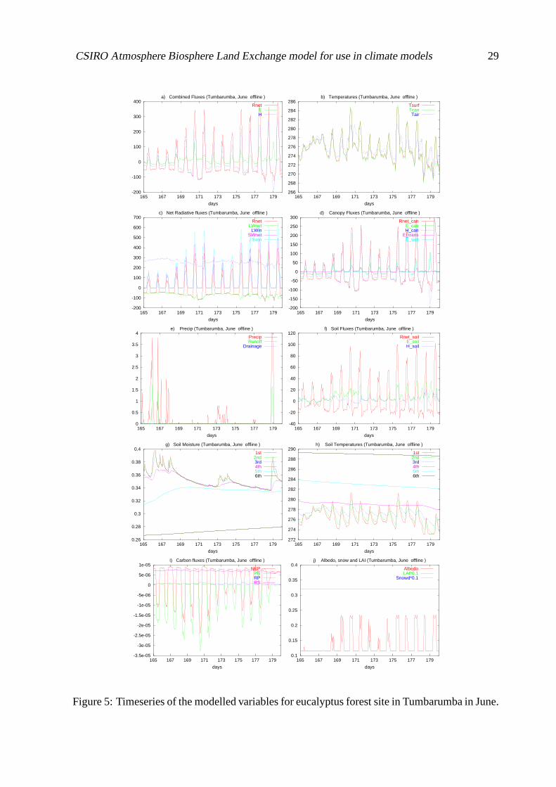
Figure 5: Timeseries of the modelled variables for eucalyptus forest site in Tumbarumba in June.


5 10 15 20 25 30

−20

−10

0

10

µmol

m−

2

NEE

5 10 15 20 25 30

0

200

400

600

Wm

−2

Latent heat

5 10 15 20 25 30

0

200

400

600

Sensible heat

Wm

−2

January days

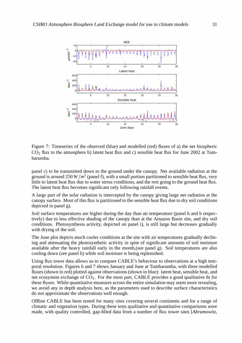
Figure 6: Timeseries of the observed (blue) and modelled (red) fluxes of a) the net biosphericCO2 flux to the atmosphere b) latent heat flux and c) sensible heat flux for January 2002 atTumbarumba.

of the model. CABLE’s parameters and initial values for these simulations were taken from thesame global fields as for the coupled run mentioned above. That is, each site’s parameters weretaken to be those representing the two by two degree grid box which contains the site. For eachgrid box initial model state values were derived from an equilibrium state of a coupled modelsimulation.

Half-hourly atmospheric forcing for the first site comes from the measurements at the eddy co-variance flux tower site in Tharandt, a coniferous forest site in north eastern Germany. Tharandtwas prescribed as a needle-leaf evergreen tree site with medium clay soil type.

Tharandt meteorological input data was measured during 1996. Although in April the radiationfluxes are relatively high (see panel c), the snow still covers the ground reflecting back a part ofthe solar radiation. Panel j) shows the evolution of snow cover starting from a small snow depth,through fast snow melt due to above zero air temperatures (panel b) and rainfall (panel e) whichaccelerates melting of the snow. Soil moisture is frozen initially but unfreezes gradually withthawing snow and soil (panel g). The top two soil temperatures reached melting stage withintwo days, while the third and fourth layers melted four and nine days later respectively (panelh).

Panel d) shows the canopy available radiation partitioned to sensible heat flux and small evap-oration flux. For the first ten days the transpiration flux is being inhibited by frozen soil butrecovers in the last four days with the thawing of the ground. Similarly, carbon fluxes depictedon panel i) are initially composed of respiration followed by onset of photosynthesis.

Figure 4 shows January model output for Tumbarumba, a eucalypt forest site in south easternAustralia. The hourly meteorological input data to CABLE was measured at the flux towersduring 2002. Tumbarumba’s eucalyptus forest was represented in the coupled simulation as abroad-leaf evergreen tree site with medium clay soil. The prescribed canopy at Tumbarumba isnot very dense (LAI 2.8) which allows a large portion of the incoming solar flux (depicted in


5 10 15 20 25 30

−20

−10

0

10

µmol

m−

2

NEE

5 10 15 20 25 30

0

200

400

600

Wm

−2

Latent heat

5 10 15 20 25 30

0

200

400

600

Sensible heat

Wm

−2

June days

Figure 7: Timeseries of the observed (blue) and modelled (red) fluxes of a) the net biosphericCO2 flux to the atmosphere b) latent heat flux and c) sensible heat flux for June 2002 at Tum-barumba.

panel c) to be transmitted down to the ground under the canopy. Net available radiation at theground is around 250 W

�m2 (panel f), with a small portion partitioned to sensible heat flux, very

little to latent heat flux due to water stress conditions, and the rest going to the ground heat flux.The latent heat flux becomes significant only following rainfall events.

A large part of the solar radiation is intercepted by the canopy giving large net radiation at thecanopy surface. Most of this flux is partitioned to the sensible heat flux due to dry soil conditionsdepicted in panel g).

Soil surface temperatures are higher during the day than air temperature (panel h and b respec-tively) due to less effective shading of the canopy than at the Amazon Basin site, and dry soilconditions. Photosynthesis activity, depicted on panel i), is still large but decreases graduallywith drying of the soil.

The June plot depicts much cooler conditions at the site with air temperatures gradually declin-ing and attenuating the photosynthetic activity in spite of significant amounts of soil moistureavailable after the heavy rainfall early in the month,(see panel g). Soil temperatures are alsocooling down (see panel h) while soil moisture is being replenished.

Using flux tower data allows us to compare CABLE’s behaviour to observations at a high tem-poral resolution. Figures 6 and 7 shows January and June at Tumbarumba, with three modelledfluxes (shown in red) plotted against observations (shown in blue): latent heat, sensible heat, andnet ecosystem exchange of CO2. For the most part, CABLE provides a good qualitative fit forthese fluxes. While quantitative measures across the entire simulation may seem more revealing,we avoid any in depth analysis here, as the parameters used to describe surface characteristicsdo not approximate the observations well enough.

Offline CABLE has been tested for many sites covering several continents and for a range ofclimatic and vegetation types. During these tests qualitative and quantitative comparisons weremade, with quality controlled, gap-filled data from a number of flux tower sites [Abramowitz,


2005; Wang et al., 2006].

4.1 Climate-carbon feedback simulations.

The carbon fluxes, photosynthesis (An), leaf respiration (Rd), plant respiration (Rp) and soilrespiration (Rs), are output each timestep by CABLE. These fluxes can be aggregated in timeto provide estimates of gross primary production, ΦGPP, net primary production, ΦNPP, and netecosystem production, ΦNEP.

ΦGPP � An � Rd (131)

ΦNPP � An � Rp (132)

ΦNEP � An � Rp � Rs (133)

The fluxes can also be used to model atmospheric CO2 when coupled to C-CAM or anotheratmospheric model.

The net biospheric flux to the atmosphere is ΦNEE � Rp � Rs � An. Flux units are gCm� 2s

� 1.Flux is input to the lowest model level and converted to a change in concentration in the surfacelayer, ∆C in ppm, using

∆C � 1000 ΦNEE g ∆t Mair

MC ∆σ ps(134)

where g is the acceleration due to gravity, ∆t is the model timestep (s), ∆σ is the fraction of theatmospheric column that makes up the lowest model level, ps is surface pressure � Pa � , Mair andMC are the molecular masses of ‘air’ and carbon respectively.

After input to the atmosphere, the CO2 is transported as a passive tracer, being subject to ad-vection by the resolved winds and sub-grid scale transport by convection. Providing other com-ponents of the carbon cycle such as fossil emissions and ocean exchange are also modelled orprescribed, the total modelled CO2 concentration can be used as input to CABLE and/or to C-CAM’s radiation scheme. This enables climate-carbon feedbacks to be assessed but this has notbeen done for the fully coupled system. However, two preliminary tests have been performed.The first followed the C4MIP Phase 1 experimental protocol and used observed global CO2 forboth CABLE and the radiation scheme. The experiment is described in Law et al. [2006] andbriefly below. The second used the modelled CO2 for CABLE but used the prescribed globalCO2 for the radiation scheme.

The C4MIP experiment simulated the twentieth century using prescribed sea surface tempera-tures and global CO2. This ensured a climate simulation with close to observed trends. CABLEresponded to the increasing CO2 and changing climate with increased ΦGPP, ΦNPP and respi-ration across the century (Fig. 8). At the end of the century the ΦNEE was a small sink of CO2out of the atmosphere. The modelled atmospheric CO2 was assessed for the last four decadesof the simulation. A detailed presentation of the results is given in Law et al. [2006]. Here wesummarise the main features. The results showed a reasonable simulation of the CO2 growthrate over the last two decades. The seasonal cycle of CO2 (first detrended using a smoothingspline) was well simulated in the northern high latitudes (e.g. Barrow, Alaska, Fig. 9a) but un-derestimated at mid-latitudes (e.g. Ulaan Uul, Mongolia, Fig.9b). There are limited samplingsites in the tropics but the seasonality at Cape Rama, India, a location strongly influenced by themonsoon, was well simulated (Fig. 9c). Seasonal cycles are small in the southern hemispherebut the phasing was incorrect at all sites (e.g. South Pole, Fig. 9d). The north-south CO2 gra-dient was overestimated due to a northern mid-high latitude biospheric source and a southernlow-mid latitude biospheric sink. A small sample of diurnal cycles suggested that respirationfluxes are too large, at least at the sampled locations. The final 40 years of the C4MIP experi-


Figure 8: Gross primary production (ΦGPP) (top), plant respiration (Rp) (middle) and soil respi-ration (Rs) (bottom) for the C4MIP simulation (blue) and the simulation in which CABLE wasforced with variable CO2 (red).

ment were repeated with CABLE forced by modelled rather than prescribed CO2. The globalgrowth rate of CO2 can be approximated by the results from a single, remote site such as MaunaLoa, Hawaii. In the first decade of the simulation forced with modelled CO2, the Mauna LoaCO2 concentration increased more rapidly than in the C4MIP experiment (Fig. 10). However,from about 1975 the growth rate decreased and by 2000, the atmospheric CO2 was about 12 ppmlower than in the C4MIP case (and closer to observed concentrations). This can be explainedby looking at the carbon fluxes (Fig. 8). Each carbon flux increases over the century and showsinterannual variability. ΦGPP (photosynthesis) from the variable CO2 run is larger than from theC4MIP run for the 1970s and 1980s. This is because photosynthesis increases as atmosphericCO2 increases (the so-called “fertilization effect”) and during the 1970s and 1980s the run usingmodelled CO2 has higher concentrations than those prescribed in the C4MIP run. Note that theprescribed concentrations in the C4MIP run are based on observed concentrations and are lowerthan the modelled concentrations in the C4MIP case. The larger ΦGPP fluxes in the 1970s and1980s create an increased sink for atmospheric CO2. This contributes to a slowing of the CO2growth rate and the return of CO2 concentrations to observed levels. Consequently in the 1990sthe ΦGPP fluxes are similar for both simulations.

Plant respiration (Rp, Fig. 8b) shows similar behaviour although both the fluxes and the fluxdifferences are smaller in magnitude. Plant respiration does not respond to atmospheric CO2directly, but rather to increasing plant pool sizes which are determined by ΦGPP. The resultsfor soil respiration (Rs) are harder to explain. Fig. 8c shows that Rs is initially larger in thevariable CO2 case than in the C4MIP simulation and then becomes smaller than the C4MIPvalues. Soil respiration is driven by soil temperature and moisture as well as the fast carbonpool size. In the variable CO2 case, the fast carbon pool decreases slightly in the early 1960sthen increases through the rest of the simulation. This would imply that Rs fluxes are opposite


Figure 9: Observed (blue) and modelled (green) seasonal cycle of atmospheric CO2 for foursites, Barrow (157oW, 71oN) (a), Ulaan Uul (111oE, 44oN) (b), Cape Rama (74oE, 15oN) (c) andSouth Pole (d). Model results for CABLE also include fossil, land-use and ocean contributionsto seasonality. The interannual variability in the observed seasonal cycle is shown by the blueerror bars.

Figure 10: Observed (blue) and modelled atmospheric CO2 concentration at Mauna Loa, Hawaiifor the C4MIP simulation (green) and the simulation in which CABLE was forced with variableCO2 (red).


to those obtained i.e. initially smaller than C4MIP and then larger. It is possible that trendsin temperature and moisture dominate over the change in pool size, but there appears to belittle evidence for significantly different trends in temperature and moisture between the twosimulations. The C4MIP and the variable CO2 simulations were performed many months apartwith a 2003 version of C-CAM. It may be that a small change was made to the Rs formulationbetween the two simulations negating a clean comparison. In a future study, we plan to repeatthese simulations with the current version of CABLE/C-CAM in order to check the results.

5 Final comments

We have described a biosphere atmosphere exchange model that forms the basis of a land surfacescheme which is being incorporated into C-CAM and ACCESS GCMs. This model, togetherwith surface data sets forms Phase I of a longer term plan to improve representation of surfaceprocesses in the CSIRO and ACCESS GCMs. Together with the basic description of the model,we have provided examples of the model performance.

6 Acknowledgments

We thank the Australian Greenhouse Office for their contribution to funding the work in develop-ing CABLE. We also thank Mike Raupach, Ray Leuning and Klara Finkele (former CSIRO em-ployee) for their significant contributions during various stages of CABLE development. AshokLuhar and Peter Hurley provided valuable comments on the manuscript.

References

Abramowitz, G., Towards a benchmark for land surface models, Geophys. Res. Letts., 32,L22,702, 2005, doi:10.1029/2005GL024419.

Clapp, R. B., and G. M. Hornberger, Empirical equations for some soil hydraulic properties,Water resources research, 14, 601–604, 1978.

Deardorff, J. W., A parameterization of ground-surface moisture content for use in atmosphericprediction models, J. Appl. Meteorol., 16, 1182–1185, 1977.

Deardorff, J. W., Efficient prediction of ground surface temperature and moisture, with inclusionof a layer of vegetation, J. Geophys. Res., 83, 1889–1903, 1978.

Dickinson, R. E., M. Shaikh, R. Bryant, and L. Graumlich, Interactive canopies for a climatemodel, J. Climate, 11, 2823–2836, 1998.

Durran, D., Numerical methods for wave equations in GFD, Springer Verlag, New York, 1999.

Finkele, K., J. J. Katzfey, E. A. Kowalczyk, J. L. McGregor, L. Zhang, and M. R. Raupach,Modelling of the OASIS energy flux measurements using two canopy concepts, Boundary-Layer Meteor., 107, 49–79, 2003.

Garratt, J. R., The atmospheric boundary layer, Cambridge University Press, 1992.


Gordon, H. B., et al., The CSIRO Mk3 Climate System Model, CSIRO Atmospheric Researchtechnical paper 60, 2002, (electronic publication).

Goudriaan, J., and H. H. van Laar, Modelling crop growth processes, Kluwer, Amsterdam, TheNetherlands, 1994.

Hillel, D., Introduction to soil physics, Academic Press, 1982.

Johansen, O., Thermal conductivity of soils, Ph.D. thesis, University of Trondheim, 1975.

Kowalczyk, E. A., J. R. Garratt, and P. B. Krummel, A soil-canopy scheme for use in a numericalmodel of the atmosphere - 1D stand-alone model, CSIRO Division of Atmospheric Researchtechnical paper 23, 1991.

Kowalczyk, E. A., J. R. Garratt, and P. B. Krummel, Implementation of a soil-canopy schemeinto the csiro gcm - regional aspects of the model response, CSIRO Atmospheric Researchtechnical paper 32, 1994.

Law, R. M., E. A. Kowalczyk, and Y. P. Wang, Using atmospheric co2 data to assess asimplified carbon-climate simulation for the 20th century, Tellus, 53B, 427–437, 2006,doi:10.1111/j.1600-0889.2006.00198.x.

Leuning, R., Modelling stomatal behaviour and photosynthesis of eucalyptus grandis, Aust. J.Plant Physiol., 17, 159–175, 1990.

Leuning, R., Temperature dependence of two parameters in a photosynthesis model, Plant CellEnviron., 25, 1205–1210, 2002.

Leuning, R., F. M. Kelliher, D. G. G. De Pury, and E.-D. Schulze, Leaf nitrogen, photosynthesis,conductance and transpiration: scaling from leaves to canopies, Plant Cell Environ., 18, 1183–1200, 1995.

Louis, J. F., A parameteric model of vertical eddy fluxes in the atmosphere, Bound. Layer Me-teor., 17, 187–202, 1979.

Monin, A. S., and A. M. Obukhov, Basic laws of turbulent mixing in the atmosphere near theground, Tr. Geofiz. Inst., Akad. Nauk SSSR, 24, 163–187, 1954.

Paulson, C. A., The mathematical representation of wind speed and temperature profiles in theunstable atmospheric surface layer, J. Appl. Meteor., 9, 857–861, 1970.

Raupach, M. R., Applying lagrangian fluid-mechanics to infer scalar source distributions fromconcentration profiles in plant canopies, Agric. Forest Meteor., 47, 85–108, 1989a.

Raupach, M. R., A practical lagrangian method for relating scalar concentrations to source dis-tributions in vegetation canopies, Quart. J. Roy. Meteor. Soc., 115, 609–632, 1989b.

Raupach, M. R., Simplified expressions for vegetation roughness length and zero-plane displace-ment as functions of canopy height and area index, Boundary-Layer Meteor., 71, 211–216,1994.

Raupach, M. R., K. Finkele, and L. Zhang, SCAM (Soil-Canopy-Atmosphere Model): descrip-tion and comparison with field data, CSIRO Centre for Env. Mechanics Tech. Rep. 132, 1997.

Roe, P. L., Some contributions to the modelling of discontinuous flows, in Lecture notes inApplied Mathematics, vol. 22, pp. 163–193, Springer-Verlag, New York, 1985.


Spitters, C. J. T., Separating the diffuse and direct component of global radiation and its impli-cation for modelling canopy photosynthesis. Part II: Calculations of canopy photosynthesis,Agric. Forest Meteor., 38, 231–242, 1986.

Wang, Y.-P., A refinement to the two-leaf model for calculating canopy photosynthesis, Agric.Forest Meteor., 101, 143–150, 2000.

Wang, Y. P., and R. Leuning, A two-leaf model for canopy conductance, photosynthesis andpartitioning of available energy I. Model description and comparison with a multi-layeredmodel, Agric. Forest Meteor., 91, 89–111, 1998.

Wang, Y.-P., D. Baldocchi, R. Leuning, E. Falge, and T. Vesala, Estimating parameters in a land-surface model by applying nonlinear inversion to eddy covariance flux measurements fromeight FLUXNET sites, Glob. Change Biol., 12, 2006, doi:10.1111/j.1365-2486.2006.01225.x.

Documents

The CSIRO Atmosphere Biosphere Land Exchange