Embed Size (px)
Citation preview

POUR L'OBTENTION DU GRADE DE DOCTEUR ÈS SCIENCES
acceptée sur proposition du jury:
Prof. O. Schneider, président du juryProf. G. Margaritondo, directeur de thèse
Dr A. Cricenti, rapporteur Prof. G. Dietler, rapporteur Prof. N. H. Tolk, rapporteur
Biological Samples Studied by Optical Nanospectroscopy
THÈSE NO 4425 (2009)
ÉCOLE POLYTECHNIQUE FÉDÉRALE DE LAUSANNE
PRÉSENTÉE LE 19 jUIN 2009
À LA FACULTÉ SCIENCES DE BASELABORATOIRE DE PHYSIQUE DES RAYONS X
PROGRAMME DOCTORAL EN PHYSIQUE
Suisse2009
PAR
johanna GENEROSI


“We build too many walls and not enough bridges.”
Isaac Newton


i
TABLE OF CONTENTS
Table of contents ..........................................................................................................................................................i
Abstract ........................................................................................................................................................................... v
Sommario .................................................................................................................................................................... vii
List of abbreviations ............................................................................................................................................... ix
Introduction .................................................................................................................................................................. 1
1. Theory and methods ........................................................................................................................................... 5
1.1. Electromagnetic radiation and its interaction with matter ........................................................... 5
1.2. Visible light: from optical microscopy to scanning near-field microscopy ............................. 7
1.2.1. Scanning near-field optical microscopy imaging theory ........................................................ 7
1.2.2. SNOM configurations .......................................................................................................................... 13
1.2.3. Fluorescence SNOM ............................................................................................................................. 14
1.3. Infrared radiation: a tool for chemical analysis ................................................................................ 16
1.3.1. FTIR spectroscopy ................................................................................................................................ 17
1.3.2. A free electron laser as light source for an infrared collection SNOM ............................ 17
1.4. SNOM probes: theory and fabrication methods ............................................................................... 21
1.5. Basic principles of atomic force microscopy ...................................................................................... 24
1.5.1. AFM experimental stup ...................................................................................................................... 26
1.6. X-rays: from in-house source to synchrotron radiation ................................................................ 27
1.6.1. X-ray scattering ..................................................................................................................................... 27
1.6.2. Energy dispersive X-ray diffraction .............................................................................................. 30
1.6.3. X-ray reflectivity ................................................................................................................................... 31
1.6.4. Parratt formalism ................................................................................................................................. 33
1.6.5. Surface roughness ................................................................................................................................ 35
1.6.6. Diffuse scattering .................................................................................................................................. 36
1.6.7. Synchrotron radiation ........................................................................................................................ 37
1.6.6. Beamline D4 at Hasylab, Desy ......................................................................................................... 38
References ................................................................................................................................................................ 38
2. Solid supported lipid membranes ............................................................................................................ 41
2.1. Introduction ..................................................................................................................................................... 41

ii
2.1.1. Glycerophospholipids and bilayer properties .......................................................................... 41
2.1.2. Solid-supported lipid bilayers ......................................................................................................... 43
2.1.3. DOPC, DPPC and DOTAP .................................................................................................................... 44
2.2. Investigation of order and clusters in lipid multibilayers ............................................................ 46
2.2.1. Sample preparation ............................................................................................................................. 46
2.2.2. X-ray reflectivity and diffuse scattering lipid bilayer structural properties ................ 46
2.2.3. IR-SNOM localizes membrane domains ...................................................................................... 50
2.3. Lipid-Alamethycin complex characterization ................................................................................... 54
2.3.1. Alamethycin ............................................................................................................................................ 54
2.3.2. Lipid-peptide sample preparation ................................................................................................. 55
2.3.3. DPPC-Alamethicin interaction detected by EDXD................................................................... 56
References ................................................................................................................................................................ 60
3. Hippocampal neuron cells ............................................................................................................................ 63
3.1. Introduction ..................................................................................................................................................... 63
3.1.1. Synapses ................................................................................................................................................... 64
3.1.2. AMPA receptors ..................................................................................................................................... 65
3.2. Sample preparation ...................................................................................................................................... 68
3.2.1. Cell culture ............................................................................................................................................... 68
3.2.2. Acyl carrier protein (ACP) labelling .............................................................................................. 69
3.2.3. Lentiviral production .......................................................................................................................... 69
3.2.4. The fluorophore Alexa 488 ............................................................................................................... 70
3.3. AMPARs mapping with fluorescence SNOM ...................................................................................... 71
3.3.1. Why scanning near-field optical microscopy? .......................................................................... 71
3.3.2. AMPA trafficking ................................................................................................................................... 72
3.4. Details enhancement with gradient maps .......................................................................................... 76
3.5. Resolution analysis with wavelets ......................................................................................................... 79
3.6. Photobleaching-free molecule detection ............................................................................................. 85
References ................................................................................................................................................................ 89
4. Nano-Raman: approaching the nanometer-size chemical analysis ....................................... 91
4.1. The Raman effect ........................................................................................................................................... 91
4.1.1. History ....................................................................................................................................................... 91
4.1.2. The scattering process: classical and quantum approach ................................................... 91
4.1.3. Resonance Raman scattering ........................................................................................................... 97

iii
4.1.4. Surface enhanced Raman scattering ............................................................................................. 98
4.2. Near-field Raman spectroscopy ........................................................................................................... 100
4.2.1. Experimental setup ........................................................................................................................... 100
4.2.2. Porous polycrystalline glass-ceramic ........................................................................................ 102
4.2.3. Hippocampal neuron cells ............................................................................................................. 107
4.2.4. Ongoing and future work ............................................................................................................... 110
References ............................................................................................................................................................. 111
Conclusions ............................................................................................................................................................. 113
Acknowledgements ............................................................................................................................................ 117
Publications and proceedings ...................................................................................................................... 119
Curriculum Vitae .................................................................................................................................................. 121


v
ABSTRACT
The different parts of the electromagnetic spectrum result in diverse effects upon interaction with matter: according to the wavelength, the radiation has energy appropriate for the excitation of a specific physical process.
X-rays can be used as a tool to analyze the structure of matter since their wavelength is comparable with the interatomic distances. Infrared light is in the spectral region that excites molecular vibrations and is employed to investigate the chemical composition of a material. Visible radiation can study the optical properties of a sample, such as the fluorescence and the absorbance, and provide a chemical fingerprint when the inelastically scattered light is detected.
In this thesis work these light sources are used in diverse experimental approaches to study structured biological specimens, resulting in a detailed chemical and physical characterization at the atomic and molecular scale.
Conventional spectroscopy is often not enough sensitive and spatially resolved to detect specific elements or domains in a sample. The need of imaging objects on increasingly finer scales and spatially localize specific molecules, brought to combine infrared, visible and Raman spectroscopy with scanning near-field microscopy giving rise to a powerful nanospectroscopic tool used to perform simultaneous topographical measurements and optical/chemical characterizations with subwavelength resolution, overcoming the diffraction limit of light.
Our study combines X-ray diffraction and reflectivity with optical nanospectroscopy to investigate the order and clustering of lipid bilayers, the interaction between solid-supported membranes and embedded alamethicin peptides, the optical and chemical properties of hippocampal neuron cells and the trafficking mechanism of specific neuron receptors. Keywords: near-field microscopy, nanospectroscopy, X-rays, model membranes, neuron cells


vii
SOMMARIO
Gli effetti dell’interazione tra radiazione elettromagnetica e materia dipendono dalla frequenza: a seconda della lunghezza d’onda, la radiazione ha un’energia specifica tale da scatenare nel campione un processo fisico ben definito.
In particolare, i raggi X sono comunemente utilizzati per analizzare la struttura della materia, dato che la loro lunghezza d’onda è paragonabile alle distanze interatomiche. La radiazione infrarossa eccita le vibrazioni molecolari ed è usata per investigare la composizione chimica dei campioni. Lo spettro visible puó essere impiegato come sonda per analizzare le proprietá ottiche di un oggetto, come la fluorescenza o l’assorbimeto, e puó fornire un’impronta chimica se viene rilevata la radiazione diffusa anelasticamente.
In questa tesi, i raggi X, la luce infrarossa e visibile sono utilizzati in diversi approcci sperimetali come sonde per studiare a livello atomico e molecolare le proprietà chimico-fisiche di campioni biologici.
In molti casi le tecniche spettroscopiche convenzionali non sono sufficientemente sensibili a piccole concentrazioni o non hanno una risoluzione tale da poter identificare, nei campioni, determinati aggregati o domini. Il crescente bisogno di visualizzare oggetti sempre piú piccoli e di localizzare molecole ha portato alla combinazione della spettroscopia visibile, infrarossa e Raman con la microscopia a campo prossimo. Il risultato è un potente strumento nanospettroscopico che permette di acquisire simultaneamente informazioni topografiche e ottiche (o chimiche) ad una risoluzione nanometrica, superando il limite di diffrazione ottica.
Il nostro lavoro consiste nella combinazione di studi strutturali effettuati con la diffrazione e riflettivitá X con misure di nanospettroscopia ottica, per investigare l’ordine e l’aggregazione di doppi strati lipidici, l’interazione tra peptidi di alameticina e la membrana in cui sono inseriti, le proprietà ottiche e chimiche di cellule neuronali dell’ippocampo e i meccanismi di diffusione di specifici recettori neuronali. Parole chiave: microscopia a campo prossimo, nanospettroscopia, raggi X, membrane, neuroni


ix
LIST OF ABBREVIATIONS
ACP Acyl carrier protein ADP Avalanche photodiode AFM Atomic force microscope/microscopy AMPA α-amino-3-hydroxy-5-methyl-4-isoxazole-propionic acid AMPAR α-amino-3-hydroxy-5-methyl-4-isoxazole-propionic acid receptor CoA Coenzyme A CTP Ca-Ti-P based glass-ceramic Db Daubechies DOPC 1,2-Dioleoyl-sn-Glycero-3-Phosphocholine DPPC 1,2-Dipalmitoyl-sn-Glycero-3-Phosphocholine DOTAP 1,2-Dioleoyl-3-Trimethylammonium-Propane (Chloride Salt) DWT Discrete wavelet transform EDXD Energy dispersive X-ray diffrectometer/diffraction FEL Free electron laser F-SNOM Fluorescence scanning near-field optical microscope/microscopy FTIR Fourier transform infrared spectroscopy Glu Glutammate IR Infrared NMDA N-methyl-D-aspartate NMDAR N-methyl-D-aspartate receptor PMT Photomultiplier PPTase Phosphopantethein transferase PSD Position sensitive detector PSD Postsynaptic density PSPD Position-sensitive photodetector RR Resonance Raman SEM Scanning electron microscope/microscopy SERS Surface-enhanced Raman scattering/spectroscopy SNOM Scanning near-field optical microscope/microscopy SPM Scanning probe microscope/microscopy STM Scanning tunnelling microscope/microscopy TEM Transmission electron microscope/microscopy TERS Tip-enhanced Raman scattering/spectroscopy


INTRODUCTION
“Of all the Inventions none there is Surpasses the Noble Florentine's Dioptrick Glasses For what a better, fitter guift Could bee in this World's Aged Luciosity. To help our Blindnesse so as to devize a paire of new & Artificial eyes By whose augmenting power wee now see more than all the world Has ever dounn before.”
This poem, written by Henry Powers in 1661, dates back to the earliest history of microscopy. At this time, Powers’ true optimism about the great potentiality of microscopy was set against the natural philosophers fear that microscopy would reveal all that it was possible to see of the microscopic world.
In the 17th and 18th centuries, the initial fear was replaced by excitement and renewed interest in microscopy due to technical improvements, such as the achievement of a higher magnification factor and resolving power, as well as the correction of the spherical and chromatic aberration problems, that led to many discoveries in biology, medicine, palaeontology and geology.
As researchers investigated smaller and smaller objects, the invisible features became the ones of new interest: the expanding need to image objects on increasingly finer scales pushed the development of microscopy even beneath the physical limit of light diffraction.
Near-field optics has its origin in the effort of overcoming the diffraction limit of optical imaging, derived by Abbe and Rayleigh at the end of the 19th century1,2. The criterion establishes the minimum distance between two point sources at which they can still be distinguished as two separate sources, i.e. . In near-field optics, the dependence on the wavelength λ is replaced by a dependence on a characteristic length d (e.g. aperture diameter or tip diameter) of a local probe.
The original idea of using the scattered light from a tiny particle as a light source and a local probe with a small aperture to perform near-field optical imaging and overcome the diffraction limit was originally developed by Edward Hutchinson Synge. This visionary Irish scientist decided to publish his work in 19283 after an exchange of letters with Albert Einstein. In these letters, uncovered by Dennis McMullan in 19904, Synge describes an instrument incredibly close to the modern near-field microscopes. Moreover, he was also the first to propose the concept of scanning, the basic principle for scanning probe microscopy (SPM).
1 Abbe, E. Archiv f. Miroskop. Anat. 9, 413 (1873). 2 Rayleigh, Lord. Phil. Mag. 5, 167 (1896). 3 Synge, E. H. Phil. Mag. 6, 356 (1928). 4 McMullan, D. Royal Microscopical Society Proceedings 25(2), 127 (1990).

INTRODUCTION 2
Few years later Synge suggested the use of piezo-quartz crystals for an accurate and rapid scan of the sample. He estimated that a 5 µm translation could be achieved by a 250 V voltage. This is exactly the sensitivity of the piezo-electric actuators used today in SPM.
In 1956, J. A. O’Keefe, without knowing the existence of Synge’s paper, proposed a near-field scanning microscope but concluded that the construction of such an instrument was “rather remote”5.
The first experimental validation of near-field microscopy using electromagnetic radiation was performed by E. A. Ash and G. Nicholls at the University College of London. In the paper published in 1972 they show an aluminium test pattern imaged by a 1.5 mm-aperture using 10 GHz microwaves6. At a separation between aperture and plane of 0.5 mm they were able to achieve a resolution better than λ/60, clearly beyond the standard microscopy diffraction limit.
Advances in scanning probe techniques, like sample and probe manipulation with subnanometre precision and three-dimensional computer imaging from sequential line scans, brought to the realization in 1989 of the first optical scan, using visible light, in the Zurich IBM Research Laboratories by Ulrich Ch. Fischer and Dieter W. Pohl7. They used a gold coated polystyrene particle as a light source to image a metal film with 320 nm holes, demonstrating ≈ 50 nm spatial resolution. It is not surprising that these first reports of near-field imaging came from the same laboratory where Gerd Binning and Heinrich Roher developed in the early 1980s the first scanning tunnelling microscope8.
Few years later, on the basis of Synge’s idea, other experiments were carried out by Malmqvist and Hertz9, Kawata10, Anger11, and Kühn12, confirming the possibility to break the diffraction limit.
The first demonstration of near-field imaging with infrared light was performed in 1985 by Gail A. Massey using a 100 µm radiation13.
A family of new optical devices had emerged: broadly classified as near-field microscopes, they obtained enhanced resolution through very close placement of a sensing element to the objet to be imaged.
In this thesis work, we describe two different kind of scanning near-field optical microscopes (SNOM), operating in illumination and collection mode. Both setups work in almost any environment without needing any particular sample preparation. The illumination-mode SNOM, named fluorescence-SNOM in our experiments, is particularly suited to probe biological samples: apart from reaching subwavelength resolution and being a totally non-destructive technique since it does not touch the sample during scanning, fluorescence-SNOM can simultaneously provide a shear-force topographical image, a
5 O’Keefe, J. A. J. Opt. Soc. Am. 46, 359 (1956). 6 Ash, E. A., G. Nicholls. Nature 237, 510 (1972). 7 Fischer, U. Ch., D. W. Pohl. Phys. Rev. Lett. 62, 458 (1989). 8 Binning, G., H. Rohrer, C. Gerber, E. Weibel. Phys. Rev. Lett. 49, 57 (1982). 9 Malmqvist L., H. M. Hertz. Opt. Lett. 19, 853 (1994) 10 Kawata, S., Y. Inouye, T. Sugiura. Scanning optical microscope system: Jap. Pat. 3,196,945, 23 Oct. 1992. 11 Anger, P., P. Bharadwaj, L. Novotny. Phys. Rev. Lett. 96, 113002 (2006). 12 Kühn, S., U. Hakanson, L. Rogobete, V. Sandoghdar. Phys. Rev. Lett. 97, 017402 (2006). 13 Massey, G. A., J. A. Davis, S. M. Katnik, E. Omon. Appl. Opt. 24, 1498 (1985).

INTRODUCTION 3
fluorescence map of the fluorescence specimens and an optical transmission micrograph. We use the fluorescence-SNOM to study labelled hippocampal neuron cells and investigate the spatial distribution of the fluorophores on the cell body and along the neurites in order to elucidate some aspects of the still unsolved mechanism of receptor-trafficking.
Although widely used in many disciplines, infrared and Raman spectroscopy lack of sensitivity for small concentrations, often not possible to detect due to stronger signal from other specimens. The increasing need to detect impurities, domains and clusters in non-homogeneous media brought to the combination of near-field microscopy and spectroscopy giving birth to a nanospectroscopic tool that can detect chemical properties at nanometric level, while viewing the specimens reconstructing the topography point by point.
The collection-mode SNOM is combined with a tuneable free electron laser, emitting in the mid-infrared range, into a spectroscopic tool, namely IR-SNOM. In particular, studying model membranes, we show how IR-SNOM is able to localize specific chemical bonds.
The last chapter is dedicated to the new developments in nanospectroscopy, achieved taking advantage of the metalized tips − commonly used during our measurements − to enhance the collected signal. The so-called tip-enhanced near-field optical microscopy14,15 is particularly useful when coupled with Raman spectroscopy. We show that with our experimental setup the low Raman signal can be enhanced to collect the fingerprint of the chemical species under study with a subwavelength spatial resolution.
Although our main attention is dedicated to optical nanospectroscopy, in this thesis work we also present some X-ray measurements to investigate the structural properties of solid-supported lipid membranes and the local deformation of model membranes embedded with alamethicin peptides.
The use and combination of different experimental approaches result in a broad study that elucidates samples chemical and physical properties, taking advantage of the diverse effects that different parts of the electromagnetic spectrum give rise to upon interaction with matter.
14 Zenhausern, F., Y. Martin, H. K. Wickramasinghe. Science 269, 1083 (1995). 15 Novotny, L., E. J. Sanchez, X. S. Xie, Ultramicroscopy 71, 21 (1998).


CHAPTER 1
THEORY AND METHODS
1.1 Electromagnetic radiation and its interaction with matter
The Sun, the Earth, and other bodies above the temperature of absolute zero (-273.15° Celsius) radiate energy of varying wavelengths to their surrounding environment. From the Latin radiare, “to emit beams” – radiation is energy transmitted through space, as particles or electromagnetic waves, or the process of their emission.
Electromagnetic radiation is emitted in discrete units known as photons that travel at the speed of light as electromagnetic waves. Electromagnetic energy is classified by increasing energy or decreasing wavelength into radio waves, microwaves, infrared, visible light, ultraviolet, X-rays and gamma-rays (Fig. 1.1).
Waves in the electromagnetic spectrum vary in size from very long radio waves, in the size range of buildings, to very short gamma-rays, smaller than an atomic nucleus.
The different parts of the electromagnetic spectrum result in diverse effects upon interaction with matter. Each portion of the spectrum has quantum energies appropriate for the excitation of certain types of physical processes. The energy levels for all physical processes at the atomic and molecular levels are quantized, and if there are no available quantized energy levels with spacing that match the quantum energy of the incident radiation, then the material will be transparent to that radiation, and it will pass through.
Starting with low frequency radio waves that the human body, for instance, is quite transparent to, as we move upward through microwaves and infrared to visible light, tissues absorb more and more strongly: photons energy matches rotational, vibrational and electronic energy level transitions of typical molecules. As a result, the energy is absorbed and penetration depth is small. In the lower ultraviolet range, all the UV from the sun is absorbed in a thin outer layer of the skin. As we move further up into the x-ray region, the human body becomes transparent again, because most of the mechanisms for absorption are gone: the energy of the photons is so large that it does not match any electronic energy transitions in matter and so the photons are not absorbed but penetrate deeply. Only a small fraction of the

1.1 ELECTROMAGNETIC RADIATION AND ITS INTERACTION WITH MATTER 6
radiation is thus absorbed, even though the process involves the more violent ionization events.
The frequency, or wavelength, is the determining factor of the electromagnetic radiation penetrating power; nevertheless, the characteristic of the medium through which the radiation is moving is equally important. For instance, the interaction of microwaves with matter other than metallic conductors will be to rotate molecules and produce heat as result of that molecular motion. Conductors will strongly absorb microwaves and any lower frequencies because they will cause electric currents which will heat the material. Most matter, including the human body, is largely transparent to microwaves. High intensity microwaves, as in a microwave oven where they pass back and forth through the food millions of times, will heat the material by producing molecular rotations and torsions, but cannot escape from the oven because the metal, and that wire screen on the glass door prevent them from escaping.
Since light interacts differently with matter, according to the radiation wavelength and to the material nature, it is used as a tool to investigate samples chemical and physical properties.
Described by words as a conceptually simple and powerful experimental approach, the resulting data is often difficult to interpret, especially when the investigated material is composite. Generally speaking, the model characterization accuracy is inversely proportional to the system complexity.
In this thesis, X-rays, infrared and visible light are used to study structured biological specimens, resulting in a detailed chemico-physical characterization at the atomic and molecular scale and in its entirety as a living system.
Specifically, solid supported lipid membranes and hippocampal neuron cells were studied with a combination of complementary techniques: fluorescence and infrared scanning near-field optical microscopy (SNOM), Fourier transform infrared (FTIR) spectroscopy, atomic force microscopy (AFM), energy dispersive X-ray diffraction (EDXD), X-ray reflectivity. This chapter describes the main theoretical concepts at the basis of these techniques along with the experimental setups used for this thesis work.
Fig. 1.1. Scheme of the electromagnetic spectrum. Only the small range between 350 nm and 780 nm is visible to the human eye. Image from mail.jsd.k12.ca.us

1.2 VISIBLE LIGHT: FROM OPTICAL MICROSCOPY TO NEAR-FIELD MICROSCOPY 7
1.2 Visible light: from optical microscopy to near-field microscopy The use of high magnification techniques is crucial in many disciplines such as the biological sciences and materials research. Traditionally, optical techniques have been the most widely employed for these purposes given their long historical development, noninvasiveness, specificity, ease of use, and relatively low cost. However, diffraction limits the spatial resolution attainable to approximately half the wavelength of the light source used. For visible radiation, this results in theoretical resolution limit of 200-300 nm which is restrictive for many applications. This limitation motivated the development of higher resolution techniques such as scanning electron microscopy (SEM) and transmission electron microscopy (TEM) [1] along with the emergence in the early 1980s of other scanning probe techniques such as atomic force microscopy (AFM), developed by Gerd Binning and Heinrich Roher in the IBM laboratories in Zurich. [2] Scanning probe microscopes (SPMs) can be generally described as instruments where a probe (or tip) is positioned to be in contact or in near-contact with the sample surface while the interaction between the probe and the surface is monitored. By scanning the tip over the sample it is possible to record a measurement at each of the discrete points that define the field of view and obtain an image. The introduction of these and related forms of microscopy have brought great gains in resolution to the point where it is now possible to image and study single atoms.
These gains in resolution, however, have been made at the expense of the optical contrast mechanism available to light microscopy. The optical microscopy abilities, such as performing spectroscopic measurements, achieving high temporal resolution, and obtaining polarization properties, are enormously powerful and informative for many applications. Moreover, many of the higher resolution techniques demand specific sample preparation and have reduced flexibility in the possible working environments: these conditions are not so easily met by biological specimens.
AFM, on the other hand, can be used to study samples near the atomic level at ambient conditions but yields little chemical information. In order to combine the high resolution of these techniques with the sensitivity, specificity, and flexibility afforded by optical techniques, a great effort was put in the development of alternative forms of microscopy, broadly classified as near-field microscopes: the evanescent wave microscopy [3], the frustrated total internal reflection microscope, [4] the photon tunnelling microscope, [5,6] the photon scanning tunnelling microscope [7,8] and the near-field scanning optical microscope. [9,10] Though they come in a number of forms, they share one salient characteristic: they beat the diffraction limit and obtain enhanced resolution through very close placement of the object to be imaged to a sensing element that may either be a sharp point (or aperture), or a plane.
1.2.1 Scanning near-field optical microscopy imaging theory
“Near-field optics is defined as that branch of optics that considers configurations that depend on the passage of light to, from, through, or near an element with subwalength features and the coupling of that light to a second element located a subwalength distance from the first.” [11]
The development of near-field optics was a consequence of the need to overcome the optical imaging diffraction limit, discovered at the end of the nineteenth century by Ernst Karl

1.2 VISIBLE LIGHT: FROM OPTICAL MICROSCOPY TO NEAR-FIELD MICROSCOPY 8
Abbé and Lord Rayleigh. They derived that there was a limit to the sharpness of details that could be seen with an optical microscope: Rayleigh postulated that for an imaging system with a circular aperture two Airy functions in the image plane can be resolved if the central maximum of one function falls on the first zero of the other function. [12] This can be translated in the relation
(1.1)
where is the numerical aperture, is the index of refraction of the surrounding medium and is the collection angle of the optical system.
Near-field optics is based on the detection of the evanescent waves by a subwavelength aperture. The evanescent waves are formed when sinusoidal waves are (internally) reflected off an interface at an angle greater than the critical angle so that total internal reflection occurs. Evanescent waves do not propagate and can be detected only if they are perturbated and therefore are partially transformed into radiative waves.
In order to better understand the SNOM performance and functionality, the near-field microscope mechanism will be first described considering simple structures and then continuing with a configuration more closely related to SNOM devices.
The first assumption, consequence of the experimental results, is that evanescent modes have to be considered as having measurable and non-negligible effects.
Fig. 1.2. Sketch of an aperture with width larger than the wavelength illuminated by a plane wave.
Let us consider an electromagnetic wave propagating normally to the z plane where an aperture is located. [13] The simple model is shown in Fig. 1.2. At a distance greater than half of the wavelength, the field can be expressed in terms of a superposition of element waves
(1.2)
where is the Fourier transform of . The integration domain of this function is interrelated with the aperture dimensions by the equations and . The expression of the field involves its decomposition into elementary waves. Each wave vector of these waves satisfies the relation

1.2 VISIBLE LIGHT: FROM OPTICAL MICROSCOPY TO NEAR-FIELD MICROSCOPY 9
(1.3)
If the width of the slot is much smaller than the wavelength of the source, remains small in comparison with . Light propagates without undergoing any significant deviation, and stays confined within a cone whose numerical aperture is as large as the size of the aperture is small. The waves which propagate behind the aperture are propagative waves.
The smaller is the extent of the aperture, the larger is the aperture of the emerging beam (Fig. 1.3). If the width of the slot is equal to , the emerging beam fills the entire half-space. Elementary waves like are in this case generated within the half-space.
Fig. 1.3. Representation of the diffraction light from an aperture. A. The width of the slit is equal to . B. The width of the slit is .
Let us assume that the width of the aperture is smaller than . In this case, elementary waves of wave vectors, like , are diffracted from the slot. The dispersion relation has to be satisfied and restricts to be purely imaginary. The field of these waves is thus expressed as
(1.4)
where is the penetration depth associated with the evanescent waves
(1.5)
These waves do not propagate along the z axis, but remain confined within the plane. They are related to high spatial frequencies of the slot. [14]
These calculations indicate the evanescent waves existence in the vicinity of apertures with dimensions smaller than half of the wavelength.
Classical microscopes detect only propagating waves, which verify . The greatest range of possible values of k is then , and consequently the best possible resolution is . When the width of the slot is smaller than , a large part of its angular spectrum becomes evanescent and is consequently lost in the far field. A wider

1.2 VISIBLE LIGHT: FROM OPTICAL MICROSCOPY TO NEAR-FIELD MICROSCOPY 10
domain of k would allow the detection of the evanescent waves. This can be done by forcing a component of the wave vector to be imaginary. [15] The relation
(1.6)
is verified if is imaginary. If only homogeneous waves can be detected, the resolution cannot be better than as the Rayleigh criterion states. However, if can be greater than
, the resolution can be far beyond this limit.
Bouwkamp [16] suggested that at great distances the field variation is similar to an oscillating dipole emission. The development of near-field optics has led to the proposal of several models for describing the scattering of an electromagnetic wave by different structures; therefore, the physics of the field emitted by a dipole is closely related and will be hereafter described.
Fig. 1.4. Schematic of the dipole with momentum parallel to the z axis.
Following the theory of the book by Born and Wolf, [17] let us consider a linear dipole, located at the coordinate system origin, vibrating along the unit vector n (Fig. 1.4). The electric polarization satisfies the equation
(1.7)
where is the Dirac distribution and the polarizability, the latter being time-dependent.
Skipping a few steps in these calculations, the equations for the components of the electromagnetic field generated by a dipole are
(1.8)

1.2 VISIBLE LIGHT: FROM OPTICAL MICROSCOPY TO NEAR-FIELD MICROSCOPY 11
where and denote the first and second derivatives of versus . In this form, the expression of the components does not allow us to separate the terms
corresponding to propagative waves and the terms corresponding to evanescent waves. In order to differentiate the evanescent part of the field, it is necessary to assume that the dipole is surrounded by a closed surface, and then to determine the flux of the Poynting vector through this surface.
The Poynting vector P can be expressed as follows:
, (1.9)
(1.10)
Proceeding to the integration of upon a sphere of radius and retaining the real terms, we determine the average value of the energy passing through the surface of the sphere. The power emitted by the dipole in a medium with dielectric constant and magnetic constant is equal to
(1.11)
where is expressed in CGS units. The smaller is the wavelength, the higher is the emitted power. It is apparent that only the components present a nonzero contribution, which corresponds to the variation of
the energy of a spherical wave. The remaining and components represent the evanescent waves. For very small distances from the dipole, the amplitude of the evanescent field is very large and extends largely over the amplitude of the propagative field.
Everything happens as if the energy associate with the evanescent waves was leaving the source and periodically returning inside it, without being ever lost by the system.
Evanescent waves can be detected only if they are perturbated and therefore partially transformed into radiative waves. A possible approach for achieving this perturbation is by frustrating the evanescent waves from a semi-infinite medium. The first demonstration was achieved near the beginning of the twentieth century by Sélényi. [18] The experiment consisted in illuminating a fluorescent material on the surface of a semicylindrical prism. Light could be observed also at angles higher than the critical angle, comprised between and , and between and . This proved the existence of evanescent waves associated with the material fluorescence, generated inside the prism.
The presence of a surface in the vicinity of a dipole modifies the nature of its emission. In 1909, Sommerfeld recognized that the Earth acts on the evanescent part of the waves emitted by an antenna, and that the energy emitted by the antenna is absorbed by the Earth. In the presence of a medium near the dipole the dipolar emission has the same form.
The dipole can assume different orientation with respect to the interface (Fig. 1.5). Let us assume that the dipole is located within a medium 1 of refractive index , and that it lies at a distance d from the second medium of refractive index . The dipole is denoted by or depending if its momentum is parallel or perpendicular to the surface of the second medium.

1.2 VISIBLE LIGHT: FROM OPTICAL MICROSCOPY TO NEAR-FIELD MICROSCOPY 12
Fig. 1.5. Schematic of a dipole in the vicinity of an interface.
In the case where the dipole lies within a homogeneous isotropic infinite medium, the total power emitted can be expressed by (1.11). The emitted power corresponds to the propagative waves emitted by the dipole. If the field generated by the dipole s perturbated by the presence of the second medium, a part of the evanescent waves can be transformed into propagative waves. This can be demonstrated with a variety of formalisms. [19-24] Let us consider Lukosz [22] calculations, for instance.
The energy emitted by a dipole, with an arbitrary orientation, normalized with respect to an energy emitted by a dipole in the presence of a single medium is
(1.12)
where
(1.13)
Different conclusions can be drawn whether the dipole is far or close ( ) from the surface. In the first case the the light emitted by the dipole in the form of propagative waves is reflected at the interface and interferes with the emitted light. [25] Depending on the distance between the dipole and the surface, these interferences are either constructive or destructive.
In the second case ( ), the surface lies within the near-field of the dipole. If the second medium is of higher refractive index than the medium in which the dipole is located ( ), this medium frustrates the evanescent waves, thus transforming them into propagative waves. This induces a rise of the radiation of the dipole.
If ( ), the waves emitted by the dipole can be totally reflected by the second medium, while the radiation is reduced.
In conclusion, plane waves total internal reflection or a dipole light emission can generate evanescent waves. This field is confined in proximity of the dipole and does not transport any energy at great distances from the dipole. In order to obtain information about the near-field part of the evanescent field has to be transformed into propagative field through perturbation. This can be achieved by using a semiinfinite, either dielectric or metallic medium, or else a second dipole.

1.2 VISIBLE LIGHT: FROM OPTICAL MICROSCOPY TO NEAR-FIELD MICROSCOPY 13
1.2.2 SNOM configurations
Apart from the general components of a SPM, a scanning near-field optical microscope involves the use of a light source, collection optics and at least one detector. These modules can be designed in a wide variety of configurations according to the operation needs and field of study. The most common operation modes are shown in Fig. 1.6.
In collection SNOM (Fig. 1.6 A), light is collected through the aperture at the end of the fiber while illumination is provided by far-field device. In illumination mode SNOM (Fig. 1.6 B), the sample is illuminated with light from an aperture, but collected in the far-field. In illumination/collection mode SNOM (Fig. 1.6 C), the sample is illuminated with light from the aperture, and light from the sample is collected through the same aperture. In oblique illumination mode SNOM (Fig. 1.6 D), the sample is illuminated with light from the aperture, and the signal is collected obliquely with a far-field device. In oblique collection mode SNOM (Fig. 1.6 E), the sample is illuminated obliquely with a far-field device, and light is collected in the fibre after passing through the aperture. In dark-field SNOM (Fig. 1.6 F), incident light is made to totally internally reflect from substrate surface. The light is collected through an uncoated fibre placed in the near-field of the sample.
In the next section two configurations will be described in detail: illumination and collection SNOM.
Fig. 1.6. Six common SNOM configurations: A. collection; B. illumination; C. Collection/illumination; D. Oblique illumination; E. Oblique collection; and F. Dark field.

1.2 VISIBLE LIGHT: FROM OPTICAL MICROSCOPY TO NEAR-FIELD MICROSCOPY 14
1.2.3 Fluorescence SNOM
The illumination-SNOM experimental apparatus was appositely designed and assembled to study biological samples, thus enhancing the ability to work in almost any environment (air, water), as well as the totally non-invasive and non-destructive characteristics of the technique. Fig. 1.7 shows the setup scheme. A multimode Argon ion laser (Koheras GmbH, Germany) is utilized as light source. The spectrum ranges between 450 and 514 nm, allowing the desired wavelength selection using a holographic filter (Kaiser Optical Systems, USA). Conventional laser features such as polarization control, phase coherence and spectral purity are fundamental for SNOM. The resulting light passes through a chopper (Newport, USA) – with an average rotation frequency of 560 Hz – before being focalized into a single-mode silica fibre (Télefo S.p.A., Italy) through a fibre coupler (Thor Labs, USA). The other end of the fibre is tapered, coated with gold and glued on a piezo. This system is positioned a few nanometres above the sample surface and acts as an illumination point.
The SNOM system works in the constant shear-force mode, using short-range probe-sample interactions to maintain a constant shear-force between the optics fibre tip and the surface. [26,27] The tip is glued on a piezo oscillating at the resonance frequency of ~ 3.7 kHz and connected to a three-dimensional positioning system with three piezo steppers. Two steppers implement the two-dimensional (x-y) scanning parallel to the specimen surface whereas the third (z-stepper) modifies the tip-specimen distance.[28]
The vibration frequency is adjusted for each scan to match the resonance (around 3.7 kHz) of the piezo-tip system. Moreover, we adopted a frequency slightly off-resonance as recently proposed to reduce the image noise: [29] our tests did confirm a substantial noise decrease with respect to the resonance frequency.
Fig. 1.7. Experimental setup scheme of illumination SNOM.
This allows for simultaneous acquisition of topographical and optical images. The simplest interpretation of imaging in this so-called shear-force feedback mode of operation suggests
1.2 VISIBLE LIGHT: FROM OPTICAL MICROSCOPY TO NEAR-FIELD MICROSCOPY 15
that by tracking the sample profile in scanning, the optical signal is more easily decoupled from the topographical signal. In addition, although the force between the probe and the sample can be a strong function of the probe or sample material, samples of many types can be studied in this manner. Samples requiring liquid ambience, such as many biological specimens, can also be examined.
As the fibre is brought to within roughly 15 nm of the surface, the resonance is damped due to what appears to be damping forces between the tip and the sample. As the tip-sample separation goes to zero, the tip amplitude becomes zero. By keeping a constant tip oscillation amplitude, a constant tip-sample separation is maintained. Thus, while recording the distance necessary to move the sample to maintain this constant tip oscillation, a topographic image is acquired.
The scanners-piezo-tip system described above is mounted on an Olympus IX71 inverted optical microscope, [30] positioned on an air-isolated workstation (Newport, USA). This configuration enables us to easily view the specimens and position the tip on the desired area to scan. The transmitted signal through the sample is then collected with a high numerical aperture (NA=1.4) 60X oil objective (Olympus, Germany), the same used to view the specimens. The gathered light is split in two through a beamsplitter in the way that approximately 20% of the signal is detected by a photomultiplier (Hamamatsu, Japan), indicated by PMT in Fig. 1.7, and the remaining 80% is filtered and collected by an avalanche photodiode (Hamamatsu, Japan). Most of the signal is sent to the avalanche since before detection it is filtered by the combination of a high-pass and a band-pass filter (Chroma, USA) that blocks the excitation light and is transparent to the signal emitted by the excited fluorescence specimens. Avalanche photodiodes have relatively low dark counts (<25/s), require low operating voltages (<15 V), have small dimensions (roughly 5 x 5 x 10 cm) and are internally cooled (thermoelectrically). Because those diodes output a single pulse for every detected photon, they require photon counting electronics. For this reason, we use lock-in devices (Stanford Research Systems, USA) to amplify the signal coming from the PMT and the avalanche photodiode.
Lock-in amplifiers (also known as a phase-sensitive detector) [31] are used to measure the amplitude and phase of signals buried in noise, since they can extract a signal with a known carrier wave from extremely noisy environment (S/N ratio can be as low as -60 dB or even less). In essence, a lock-in amplifier takes the input signal, multiplies it by the reference signal (provided from the chopper in our case), and integrates it over a specified time, usually on the order of milliseconds to a few seconds (30 or 100 ms in our experiments). The resulting signal is an essentially DC signal, where the contribution from any signal that is not at the same frequency as the reference signal is attenuated essentially to zero, as well as the out-of-phase component of the signal that has the same frequency as the reference signal (because sine functions are orthogonal to the cosine functions of the same frequency), and this is also why a lock-in is a phase sensitive detector.
The described illumination SNOM allows to simultaneously collect topographical map, transmission and fluorescence images of the selected area.

1.3 INFRARED RADIATION: A TOOL FOR CHEMICAL ANALYSIS 16
1.3 Infrared radiation: a tool for chemical analysis
Infrared (IR) radiation spans roughly three orders of magnitude in the electromagnetic radiation: its wavelength is longer than visible light but shorter than terahertz radiation, ranging between 750 nm and 1000 µm. IR light, in particular the mid-infrared, approximately 30 - 1.4 μm (4000 - 400 cm-1), is within the spectral region that excites molecular vibrations: infrared radiation is absorbed by organic molecules and converted into energy of molecular vibration.
In IR spectroscopy, molecules are exposed to infrared radiation. When the radiant energy matches the energy of a specific molecular vibration, absorption occurs. Each chemical bond in a molecule vibrates at a frequency which is characteristic of that bond; the recorded spectrum is like a fingerprint of the sample, since a given molecule absorbs only at specific wavelengths. These properties make infrared spectroscopy one of the most sensitive chemical analysis techniques.
In the particle model of electromagnetic radiation a wave consists of photons and the energy of an electromagnetic wave is quantized. The energy per photon is given by Planck-Einstein equation , where is the Planck constant ( ) and is equivalent to the classical frequency.
Molecular vibrational and rotational modes can be studied by infrared spectroscopy in terms of quantized discrete energy levels, e.g. , etc., as shown in Fig. 1.8. Each atom or molecule in a system must exist in one or other of these levels. In a large assembly of molecules there will be a distribution of all atoms or molecules among these various energy levels. [32]
Fig. 1.8. Vibrational energy levels. Absorption (black arrow) and emission (dotted arrow) processes are shown.
The energy levels are a function of an integer, the quantum number, and a parameter which is associated with the particular atomic or molecular process related with that state. When a molecule interacts with radiation, a photon is either emitted or absorbed. The energy of the quantum of radiation must exactly fit the energy gap, e.g. , etc. The emission or absorption frequency of radiation for a transition between the energy states
is given by: . Associated with the uptake of energy is the deactivation mechanism where the atom or molecules returns to its original state, emitting energy. Both mechanisms are represented in Fig. 1.8.
Any molecule has a number of stacks of energy levels, with each stack corresponding to a particular process. Roughly speaking, a molecular energy state is the sum of an electronic, vibrational, rotational and nuclear component, such as

1.3 INFRARED RADIATION: A TOOL FOR CHEMICAL ANALYSIS 17
. For every stack, each molecule must exist in one or other of these energy levels. The relative molecule population , in any two energy levels is given by the Maxwell-Boltzmann equation as follows:
(1.14)
where are the number of permitted states with energy , is the difference in energy between the states , k is the Boltzmann constant, and T is the absolute temperature.
A molecule can be considered a system of masses joined by bonds with spring-like properties. In the simple case of a diatomic molecule, only one vibration is possible, which corresponds to the stretching and compression of the bond. This accounts for one degree of vibrational freedom. Polyatomic molecules, with N atoms will have 3N degrees of freedom, distributed into translational, rotational and vibrational. Linear molecules, such as CO2, have 3N-5 vibrational degree of freedom, while non-linear molecules, such as H2O, have 3N-6. Vibrations can either involve a change in the bond length – stretching – or bond angle – bending. Some bonds can stretch in-phase – symmetric stretching – or out-of-phase – asymmetric stretching.
The complexity of an infrared spectrum arises from the coupling of vibrations over a large part or, in some cases, over the complete molecule. Such vibrations are called skeletal vibrations. Bands associated with skeletal vibrations are likely to conform to a fingerprint, of the molecule as a whole rather then to a specific group within the molecule.
In this work, IR spectroscopy measurements were performed using two different experimental setups:
• A Fourier transform infrared (FTIR) spectrometer using a conventional source.
• An infrared near-field microscope (IR-SNOM) based on a free electron laser.
The techniques are described in detail in the next two sections.
1.3.1 FTIR spectroscopy
The FTIR spectrometer (Jasco, Japan) is composed basically of the following parts: infrared source, Michelson interferometer, sample compartment and detector. The infrared radiation passes first through the interferometer, then through the sample. During the passage, characteristic signals are measured and stored digitally in the computer. The desired IR spectrum is obtained by a Fourier transformation of these data.
1.3.2 A free electron laser as light source for an infrared collection SNOM
In a Free-Electron Laser (FEL) high energy electrons move inside a vacuum tube while magnets cause them to wiggle and produce light. Similarly to the emitted radiation in a
1.3 INFRARED RADIATION: A TOOL FOR CHEMICAL ANALYSIS 18
synchrotron radiation storage ring, the FEL produces a high intensity (infrared) beam additionally tunable across the spectrum.
In his PhD thesis in 1970, John Madey proposed the idea of the free-electron laser. [33] In 1977, together with his research group he developed at Stanford University the world first free-electron laser. Later, in 1984, an evolution of the previous FEL - the more robust Mark III FEL [34] - was constructed and designated to perform material science and medical research at Duke University. Vanderbilt University, under the national Medical Free-Electron Laser (MFEL) program, commissioned a FEL, based on the Mk. III model: in 1987 Vanderbilt University Free Electron Laser Centre started to be operative.
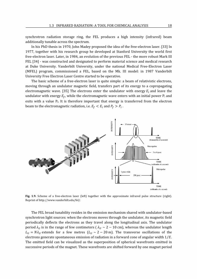
The basic scheme of a free-electron laser is quite simple: a beam of relativistic electrons, moving through an undulator magnetic field, transfers part of its energy to a copropagating electromagnetic wave. [35] The electrons enter the undulator with energy and leave the undulator with energy , while the electromagnetic wave enters with an initial power Pi and exits with a value Pf. It is therefore important that energy is transferred from the electron beam to the electromagnetic radiation, i.e. .
Fig. 1.9. Scheme of a free-electron laser (left) together with the approximate infrared pulse structure (right). Reprint of http://www.vanderbilt.edu/fel/.
The FEL broad tunability resides in the emission mechanism shared with undulator-based synchrotron light sources: when the electrons moves through the undulator, its magnetic field periodically deflects the electrons as they travel along the longitudinal axis. The undulator period is in the range of few centimeters ), whereas the undulator length
extends for a few metres ( ). The transverse oscillations of the electrons generate spontaneous emission of radiation in a forward cone of angular width . The emitted field can be visualized as the superposition of spherical wavefronts emitted in successive periods of the magnet. These wavefronts are shifted forward by one magnet period

1.3 INFRARED RADIATION: A TOOL FOR CHEMICAL ANALYSIS 19
along the direction of motion for each successive period traversed by the electrons, yielding an assembly of nested spherical wavefronts [36,37] with a well defined wavelength equal to the wavefront spacing along the emission angle. The periodic transverse motion of the electrons in the magnet thus transforms the broad white synchrotron radiation light emitted by electrons in a simple dipole field into monochromatic light. The wavefront spacing depends on the average electron velocity, which in turn depends on both the magnetic field strength and the electron energy, and these latter two parameters can be varied continuously to tune the laser.
We performed IR-SNOM measurement using the Vanderbilt University (VU) free electron laser facility. VU FEL provides tunable IR light from 2 to 10 microns wavelength with high output power and brightness. The electron beam is produced by a 45-MeV-radiofrequency accelerator operating at a frequency up to 2.856 GHz. Pulses have an average duration of 6 µs, 360 mJ energy, 11 W average power and a repetition rate of 30 Hz. [38] Fig. 1.9 shows the basic scheme of VU FEL together with the pulse characteristics.
The infrared collection SNOM setup is shown in Fig. 1.10 B. The FEL radiation follows the optical path sketched in panel A: the IR beam is reduced in power to through an eyepiece, reflected by mirrors and focalized by an optical lens on a sample area of ~1 mm2. The use of a semi-transparent Germanium filter, that cuts the HeNe line – useful for optical alignment – and laser higher orders, permits to record the reference signal for each scanned point: although the FEL light is very stable, small fluctuations in intensity are still present; each SNOM map can be thus normalized by the reference matrix, excluding the presence of artifacts due to intensity variation in the illumination beam. The SNOM [27] is a two piece cylinder: the detection system is attached to the upper part while the sample scanning device is in the lower part. The sample is mounted on a sample holder which can move in the 3 spatial direction x, y and z due to piezoelectric scanners. For bigger steps, two additional motors allow the sample to move ± 4 mm in the x-y plane, with a minimal step of 1 micron. The scanning procedure, the electronics description and the data acquisition mechanism is the same as for the fluorescence SNOM (section 1.2.3). To avoid redundancies, they will not be mentioned here.
Fig. 1.10. Scheme of the experimental setup of the infrared SNOM. A. Optical path of the FEL beam aimed to focus the infrared light onto 1 mm2 area of the sample. B. Sketch of the collection SNOM.

1.3 INFRARED RADIATION: A TOOL FOR CHEMICAL ANALYSIS 20
After illumination, the reflection is collected through a very small aperture in a gold-coated chalcogenide fiber (US Navy [39]). The incidence angle is 10-15° (found to be the best for the reflectance ratio maximum sensitivity [40]), while the collection is at 90°, with respect to the horizontal plane. The reflected signal is then detected by a HgCdTe nitrogen cooled photodiode (EOS, USA) amplified and detected by a boxcar. The surface of the sample is scanned simultaneously (scanning area up to 30 µm x 30 µm), so for each point we collect topographical and optical information.
1.4 SNOM PROBES: THEORY AND FABRICATION METHODS 21
1.4 SNOM probes: theory and fabrication methods
The development of lasers in the 1960s led to new interest in optics. This was amplified when it was discovered that silica fibres could guide light with losses of the order of dB/km.
The evanescent field itself is not actively involved in the guiding of the light. Rather, the evanescent field can be regarded as reflecting the fact that the light is being guided. The propagation of light inside an optical fibre can be analyzed in terms of ray-optical arguments [41]. The relative variations of indices inside the fibres are generally smaller than one, and therefore the theory of paraxial rays can be applied here.
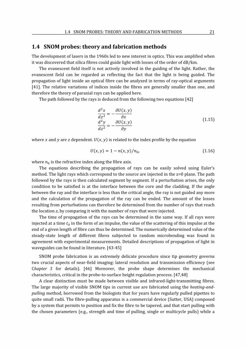
The path followed by the rays is deduced from the following two equations [42]
(1.15)
where is related to the index profile by the equation
, (1.16)
where is the refractive index along the fibre axis. The equations describing the propagation of rays can be easily solved using Euler’s
method. The light rays which correspond to the source are injected in the z=0 plane. The path followed by the rays is then calculated segment by segment. If a perturbation arises, the only condition to be satisfied is at the interface between the core and the cladding. If the angle between the ray and the interface is less than the critical angle, the ray is not guided any more and the calculation of the propagation of the ray can be ended. The amount of the losses resulting from perturbations can therefore be determined from the number of rays that reach the location z, by comparing it with the number of rays that were injected.
The time of propagation of the rays can be determined in the same way. If all rays were injected at a time in the form of an impulse, the value of the scattering of this impulse at the end of a given length of fibre can thus be determined. The numerically determined value of the steady-state length of different fibres subjected to random microbending was found in agreement with experimental measurements. Detailed descriptions of propagation of light in waveguides can be found in literature. [43-45]
SNOM probe fabrication is an extremely delicate procedure since tip geometry governs two crucial aspects of near-field imaging: lateral resolution and transmission efficiency (see Chapter 3 for details). [46] Moreover, the probe shape determines the mechanical characteristics, critical in the probe-to-surface height regulation process. [47,48]
A clear distinction must be made between visible and infrared-light-transmitting fibres. The large majority of visible SNOM tips in current use are fabricated using the heating-and-pulling method, borrowed from the biologists that for years have regularly pulled pipettes to quite small radii. The fibre-pulling apparatus is a commercial device (Sutter, USA) composed by a system that permits to position and fix the fibre to be tapered, and that start pulling with the chosen parameters (e.g., strength and time of pulling, single or multicycle pulls) while a

1.4 SNOM PROBES: THEORY AND FABRICATION METHODS 22
carbon dioxide laser heats the fibre. By changing the mentioned parameters, it is possible to produce different tapers with different shapes.
The probes were fabricated from singlemode telecommunication silica optical fibres (Télefo S.p.A., Italy), with a 4.7 µm core diameter, 100 µm glass and 125 µm polymer cladding. The polymer cladding was removed with dicloromethane and the exposed silica core was positioned in the focus of the CO2-laser beam. The shape and aperture size of the resulting tapers can vary: 50 nm apertures were achieved by optimizing the fibre-pulling system parameters. Fibres were finally coated with a 100 nm layer of gold through a metal evaporator. A sketch is shown in Fig. 1.11.
Fig. 1.11. Sketch of a gold coated SNOM probe. In the apex region, the field amplitude is attenuated and the metal coating gives rise to significant field dissipation due to absorption.
IR-SNOM probes were fabricated from singlemode chalcogenide (arsenic sulphide) fibres. Chalcogenides fibres have a good chemical stability and are less brittle than the other families of compounds from which IR fibres have been made. Nevertheless, this kind of fibres still remains very fragile and difficult to handle. Thus, the heating-and-pulling system, easy to use, fast and reliable for silica fibres, would be difficult to use. Therefore, we chemically etched the chalcogenide fibres following the method described by Unger et al. [49]
Infrared SNOM probes were fabricated from singlemode arsenic sulphide fibres, provided by the US Navy, [39] with an outside diameter varying between 80 and 140 µm and a core of 10 µm. The chemical etching consisted first in the cladding removal and then in the core etching. The cladding was removed by dipping 3 cm of the polyamide-stripped fibre edge in acetone (C3H6O) for approximately 2 minutes. With the help of a razor the cladding could be removed without damaging the core inside. Once exposed, the core was immersed into a two-phase etching solution: the lower phase being the etchant solution (piranha solution: a 7:3 mixture of concentrated sulphuric acid and 30% hydrogen peroxide), while the upper phase being a protective solvent (tetramethylpentadecane - TMPD). A scheme of the etching procedure is shown in Fig. 1.12. Panels A and B show the tip formation mechanism, which is described by in [49] in this way: “As the etching agent dissolves the fibre, the solution density increases next to the fibre surface. Since it is more dense than the rest of the solution, it flows

1.4 SNOM PROBES: THEORY AND FABRICATION METHODS 23
down the fibre; under these conditions the flow is laminar. As it flows down the fibre, more etchant solution must move to take its place. Since there is a fluid layer moving parallel to the surface of the fibre everywhere but close to the meniscus (the “top” of where the etchant touches the fibre), new etchant solution enters the convection pattern primarily at the meniscus. Since the etchant solution contacting the fibre is more reactive (i.e. contains more H2O2 and less dissolved chalcogenide) at the meniscus, it etches faster there. This results in a necking effect. Eventually the neck will be dissolved completely way, and the fibre below the neck will fall”.
The TMPD protective layer makes the tip shape more reproducible and smooth. The average etching time is 30-40 minutes.
Fig. 1.12. Schematic of the two-phase etching mechanism: A. The piranha solution starts etching the core. B. After 30-40 minutes, part of the fibre falls down leaving a smooth, concave-conical tip. C. Zoom onto a chalcogenide etched fibre.

1.5 BASIC PRINCIPLES OF ATOMIC FORCE MICROSCOPY 24
1.5 Basic principles of atomic force microscopy
Atomic force microscopy (AFM) is a high-resolution surface characterizing technique. Differently from scanning tunnelling microscopy (STM), it has the advantage of imaging almost any type of surface, including polymers, ceramics, composites, glass, and in particular biological samples. [50,51]
AFM can operate on conducting and non-conducting surfaces and is based on the existence of a separation dependency force between a tip and the substrate that is present at a close separation.
Typically, pyramidal silicon nitride tips are used, which have a radius of curvature on the order of 100 Å. These are made by an etching process that removes silicon from the substrate, leaving an etched or sharpened tip behind. The force is detected by placing the tip on a flexible cantilever that deflects proportionally to the exerted force. The deflection is then measured by some convenient procedure, such as laser reflection (Fig. 1.13).
Fig. 1.13. Scheme of an atomic force microscope. The deflection of the cantilever is measured by laser reflection.
The interaction force consists in an attractive component, the Van der Waals force, and a repulsive one, the Pauli force. To describe this scenario we refer to the Lennard-Jones potential shown in Fig. 1.14. At the right side of the curve the atoms are separated by a large distance. As the atoms are gradually brought together, they first weakly attract each other. This attraction increases until the atoms are so close together that their electron clouds begin to repel each other electrostatically. This electrostatic repulsion progressively weakens the attractive force as the interatomic separation continues to decrease. The force goes to zero when the distance between the atoms reaches a couple of ångströms, about the length of a chemical bond. When the total force becomes positive (repulsive), the atoms are in contact.
The slope of the Lennard-Jones potential is very steep in the repulsive or contact regime. As a result, the repulsive force balances almost any force that attempts to push the atoms closer together. In AFM this means that when the cantilever pushes the tip against the sample, the cantilever bends rather than forcing the tip atoms closer to the sample atoms. Even if you design a very stiff cantilever to exert large forces on the sample, the interatomic separation

1.5 BASIC PRINCIPLES OF ATOMIC FORCE MICROSCOPY 25
between the tip and sample atoms is unlikely to decrease much. Instead, the sample surface is likely to deform.
In addition to the repulsive force described above, two other forces are generally present during contact AFM operation: a capillary force exerted by the thin water layer often present in an ambient environment, and the force exerted by the cantilever itself.
Fig. 1.14. Lennard-Jones potential: the interaction force is plot versus tip-to-sample distance.
Our measurements were conducted mostly in non-contact mode since the contact between tip and sample can alter the sample surface, especially when studying biological samples.
In fact, in contact mode AFM the deflection of the cantilever is sensed and compared in a DC feedback amplifier to some desired value of deflection. If the measured deflection is different from the desired value, the feedback amplifier applies a voltage to the piezo to raise or lower the sample relative to the cantilever to restore the desired value of deflection. The voltage that the feedback amplifier applies to the piezo is a measure of the height of features on the sample surface. It is displayed as a function of the lateral position of the sample. A few instruments operate in UHV but the majority operates in ambient atmosphere, or in liquids. Problems with contact mode are caused by excessive tracking forces applied by the probe to the sample. The effects can be reduced by minimizing the tracking force of the probe on the sample, but there are practical limits to the magnitude of the force that can be controlled by the user during operation in ambient environments. Under ambient conditions, sample surfaces are covered by a layer of adsorbed gases consisting primarily of water vapour and nitrogen which is 10-30 monolayers thick. When the probe touches this contaminant layer, a meniscus forms and the cantilever is pulled by surface tension toward the sample surface. The magnitude of the force depends on the details of the probe geometry, but is typically on the order of 100 nanoNewtons. This meniscus force and other attractive forces may be neutralized by operating with the probe and part of all the sample totally immersed in liquid.
As mentioned before, non-contact mode is used in situations where tip contact might alter the sample in subtle ways. In this mode the tip works 50 - 150 Å above the sample surface. Attractive Van der Waals forces acting between the tip and the sample are detected, and topographic images are constructed by scanning the tip above the surface. Unfortunately the attractive forces from the sample are substantially weaker than the forces used by contact mode. Therefore the tip must be given a small oscillation so that AC detection methods can be

1.5 BASIC PRINCIPLES OF ATOMIC FORCE MICROSCOPY 26
used to detect the small forces between the tip and the sample by measuring the change in amplitude, phase, or frequency of the oscillating cantilever in response to force gradients from the sample. For highest resolution, it is necessary to measure force gradients from Van der Waals forces which may extend only a nanometre from the sample surface. In general, the fluid contaminant layer is substantially thicker than the range of the Van der Waals force gradient and, therefore, attempts to image the true surface with non-contact AFM fail as the oscillating probe becomes trapped in the fluid layer or hovers beyond the effective range of the forces it attempts to measure.
1.5.1 AFM experimental setup
The mechanical setup of the AFM used in this work is basically the same as a collection SNOM, already described in section 1.3.2, with the difference of using a cantilever and a laser beam that bounces off the back of the cantilever onto a position-sensitive photodetector (PSPD), instead of an optical fibre glued on a vibrating piezo. As the cantilever bends, the position of the laser beam on the detector shifts. The PSPD itself can measure displacements of light as small as 10 Å. The ratio of the path length between the cantilever and the detector to the length of the cantilever itself produces a mechanical amplification. As a result, the system can detect sub-ångström vertical movement of the cantilever tip.
In order to investigate the topography of large samples a scanner with a 30 µm x 30 µm range was chosen for our home-made AFM. In our system (Fig. 1.15), three dc motors control the x, y, and z axes, allowing coarse moments over the sample (8 x 8 mm in the x-y plane) and a smooth approach in the z direction. The distance between cantilever and sample can be thus controlled either manually, with a lateral screw, or via software by moving the z-motor. Moreover, a 150X video-camera is mounted over the sample and permits to view the area to scan.
Non-contact AFM images were obtained in air with silicon Tap300Al cantilevers (BudgetSensors, USA) with Al reflex coating (40 N/m force constant) at constant scanning frequency.
Fig. 1.15. Picture of the atomic force microscopy experimental setup.

1.6 X-RAYS: FROM IN-HOUSE SOURCE TO SYNCHROTRON RADIATION 27
1.6 X-rays: from in-house source to synchrotron radiation
An X-ray source can be used as a probe to study the atomic structure of a sample, since its wavelength is comparable with the interatomic distances.
Discovered by W. C. Röntgen in 1895 as a new type of radiation, X-rays were immediately used in diagnostic radiology and closely related fields. However, the nature of X-rays remained unknown until 1912, when Max von Laue, studying the interaction of the radiation with three-dimensional crystals, proposed the X-ray diffraction theory, for which he won the Nobel Prize two years later.
The investigation of surfaces and interfaces with x-ray scattering methods is a field that has grown enormously in the last three decades. Increasing surface quality, technological developments concerning sophisticated surface diffractometers, synchrotron radiation facilities and a steady development of surface scattering theory have made this progress possible. Nowadays detailed and precise results from various liquid, glassy, and solid surfaces are available, and even complex layer structures can be characterized. [52]
1.6.1 X-ray scattering
Let us consider an X-ray beam that propagates along the x axis, [53] perpendicular to the electric field E, and to the magnetic field B (Fig. 1.15).
Fig. 1.15. Rapresentation of an X-ray beam as an electromagnetic wave: the electric and magnetic fields are perpendicular to the propagation direction.
The electromagnetic radiation interact mainly with the electrons and more weakly with the atoms nuclei. The most relevant interaction is therefore between the electric field and the charges; the magnetic field contribution can be neglected and the electric field can be expressed as
, (1.17)
where the unit vector indicates the electric field polarization and k is the wave vector along the propagation direction. Taking advantage of the electromagnetic waves properties,

1.6 X-RAYS: FROM IN-HOUSE SOURCE TO SYNCHROTRON RADIATION 28
. In agreement with the classic theory, these equations describe a plane linearly polarized wave.
In quantum mechanics, a monochromatic beam is composed by quantum particles, i.e. photons with energy and momentum . The beam intensity, given by the number of photons passing through a surface per unit time, is proportional to the square of the electric field. The wavelength is inversely proportional to the photon energy E:
(1.18)
Photons interact with atoms in two different ways: they can either be diffused or absorbed.
When X-rays interacts with an electron, the beam is diffused. This phenomenon is called scattering. Classically, the electric field of the incident ray interacts with the electron charge. The electron is subsequently accelerated and radiates. If the diffused beam wavelength equals the wavelength of the incident radiation the scattering is called elastic. If part of the energy is transferred to the electron instead, the scattering is inelastic (Compton effect).
The phenomenon of X-ray scattering grows in complexity starting from the scattering from an isolated, stationary atom, passing to the scattering from a molecule and finally to a crystal. Without entering into the theoretical details, explained elsewhere [53], in the following paragraph some diffraction concepts will be described in order to have a theoretical overview of the experiments and results presented in Chapter 2.
Fig. 1.16. Diagram of the exchanged vector q. k and k’ are the wave vectors before and after the scattering process, 2θ is the total scattering angle.
Taking into account the Thomson and Debye’s classic approach to the diffraction theory, let us consider the elastic scattering of an electron by X-rays, sketched in Fig. 1.16. The exchanged vector, also called scattering vector, is expressed in Å-1 as:
(1.19)
being the total scattering angle and k the modulus of both wavevectors k and . Since the scattering is elastic, the energy E of the radiation remains unchanged during scattering. Moreover, according to the dispersion relation of an electromagnetic radiation, the modulus of the wave vector is proportional to the energy. Therefore, the wave vector can vary its direction

1.6 X-RAYS: FROM IN-HOUSE SOURCE TO SYNCHROTRON RADIATION 29
but not its modulus, i.e. the X-ray beam can change its direction but not its wavelength. Being E proportional to k it is possible to write
(1.20)
where the constant α is equal to 1.014 .
Fig. 1.17. Sketch of a 2D lattice. k and k’ are the incident and diffracted wavevectors, θ is the incdent angle, d is the distance between the lattice planes.
The defining property of a crystalline material is that it is periodic in space. When X-rays are scattered from a crystal lattice, a constructive interference of waves is achieved when Bragg’s law is satisfied:
(1.21)
where is an integer and is the incident wavelength; θ is the angle of incidence and d is the lattice planes distance (Fig. 1.17).
Two methods are available to perform a scan of q and to draw the scattered intensity profile as a function of it: [54]
• Use a monochromatic beam, e.g. a fluorescence line produced by a laboratory X-ray tube: E is fixed and an angular scan is performed (Angular Dispersive X-ray Diffraction, ADXD).
• Use a continuous spectrum radiation, e.g. the Bremmstrahlung of an X-ray tube: the scattering angle is fixed (Energy Dispersive X-ray Diffraction, EDXD).
The distinction between the two methods was made in the late sixties [55]. Although the second possibility was known since a long time, solid-state detectors did not have enough resolution to let EDXD measurements be performed, letting ADXD become the most popular technique.

1.6 X-RAYS: FROM IN-HOUSE SOURCE TO SYNCHROTRON RADIATION 30
1.6.2 Energy dispersive X-ray diffraction
In angular dispersive X-ray diffraction, the maximum q value is limited by the condition of equation 1.19. Moreover, this limit can be hardly reached because of mechanical
difficulties in approaching the back scattering configuration (the X-ray tube and the detector would be in contact). [54]
In energy dispersive X-ray diffraction, instead, once the scattering angle is fixed, is determined by the highest energy component contained in the white spectrum. For example, if the power supply voltage is 50 kV, the maximum energy is, by definition, 50 keV; at an angle of 40°, theoretical equals 30 (Fig. 1.18).
Fig. 1.18. Intervals of reciprocal space that can be theoretically explored at different θ, using a white X-ray primary beam with energetic components up to 50 KeV.
There are several advantages in using an EDXD instead of an ADXD apparatus:
• Reduced acquisition time: the intensity concentrated in the fluorescence line in ADXD is typically from one to two orders of magnitude lower than the intensity distributed in the entire continuous spectrum in EDXD. This is also, roughly, the ratio between the acquisition times.
• Sample stability: since the beam hits always the same point while performing the experiment, no movements compromise the alignment, and also very small samples can be used. Moreover, complex devices, such as high pressure or variable temperature cells, can be easily installed.
• Multiple acquisition: while in the ADXD spectrum points are collected in a sequential way, with a scanning rate proportional to the angular speed of the diffractometer arms, in EDXD the points are collected simultaneously at each value of q.
On the other hand some drawbacks must be noticed: the decrease in q resolution; the need of separate analysis of energy dependent phenomena, i.e. elastic and inelastic scattering, absorption, polarization; the recombination of spectra taken at different angles. [54,56]
The experimental setup of the energy-dispersive X-ray diffractometer is shown in Fig. 1.19. Details can be found in references [57,58].

1.6 X-RAYS: FROM IN-HOUSE SOURCE TO SYNCHROTRON RADIATION 31
The EDXD apparatus differs from the commonly used angular dispersive system due to the absence of a monocromathor and a goniometer. The instrument is composed by two arms contained in the vertical plane, pivoting around a single central axis. The arms are moved by two linear actuators driven by step motors and the tangent of the angles of inclination is read by two linear encoders. Both the minimum step movement and the resolution of the encoders are 1 µm, leading to a minimum angle increment and reproducibility of 0.0004°. The X-ray optical path is defined by four variable slits mounted on the arms.
Fig. 1.19. Energy dispersive X-ray diffactometer setup, located in the Biophysics Laboratory of the Physics department in the University La Sapienza, Rome, Italy. 1. X-ray tube. 2. Vertical and horizontal slits. 3. sample holder. 4. Detector.
The source is a standard 2 kW tungsten anode X-ray tube, producing a white beam with an energy ranging from 12 to 58 keV. The X-ray detection is accomplished by an EG&G high purity germanium solid-state detector connected via hardware to a personal computer running the Maestro software to visualize and record the data through a multichannel analyzer.
The energy resolution is approximately 1.5% with a maximum count rate of 10 kcounts/s. The measurement of the incident spectra is necessary to normalize the reflectivity data. It is acquired by placing the two arms in straight position (0° inclination angle) and collecting the direct beam spectrum.
1.6.3 X-ray reflectivity
X-ray reflectivity is a useful tool to analyze the structure and organization of materials deposited as thin films at the submicronic and atomic scales. [59-64]
When a beam of light, propagating in an isotropic medium with refractive index , passes through a boundary to another medium, with different index of refraction , part of the light is reflected and part is refracted (Fig. 1.20). In the classic theory of optics, Snell’s law is the formula used to describe the relationship between the angles of incidence and refraction:

1.6 X-RAYS: FROM IN-HOUSE SOURCE TO SYNCHROTRON RADIATION 32
(1.22)
Fig. 1.20. Refraction of light at the interface between two media of different refractive indices, with n2 > n1.
Let us now consider the specific case of X-rays propagating in air and impinging on the surface of a sample. During the interaction with matter, the X-ray beam change direction when passing from air to material. The refraction index for X-rays can be written as
(1.23)
where takes into account the scattering and the absorption of the material. is the energy of the incident radiation, nm is the electron classical radius, is the electron density, is the linear absorption coefficient.
Fig. 1.21. A plane electromagnetic wave with wave vector hits a surface at a grazing angle . The wave splits into a reflected ( ) and a refracted wave transmitted at the angle .
For X-rays, is positive and slightly less than unity. Passing from air ( ) to the reflecting specimen ( ), if the incident angle θi between the sample surface and the beam is smaller than the critical angle , satisfying the equation , total external reflection can occur. Since the refractive index is very close to unity, it is possible to us the Taylor approximation in , thus obtaining

1.6 X-RAYS: FROM IN-HOUSE SOURCE TO SYNCHROTRON RADIATION 33
(1.24)
When the X-ray beam hits on a perfectly smooth surface, part of the intensity is reflected and part is transmitted through the material. Following the situation shown in Fig. 1.21, we will calculate the reflectivity of the smooth vacuum/medium interface. A plane wave in vacuum, with wavevector , hits at a grazing angle θi a flat surface of a medium with refractive index . The reflected and transmitted fields can be described by with
and where the components of are given by the law of refraction.
The reflected amplitude is derived by writing the continuity of the components of the electric and the magnetic fields at the interface . This leads to the classical Fresnel relationship which gives the reflection coefficient in amplitude for the (s) and (p) polarization. The reflectivity is the modulus square of this coefficient and can be written for X-rays as
(1.25)
This expression is independent of the polarization. Since the reflectivity is only observed in specular conditions, i.e. the incident angle equals the exit angle, introducing the wavevector transfer , we have
(1.26)
1.6.4 Parratt formalism
We will now consider the case of multiple interfaces. Fig. 1.22 shows a scheme of a stratified media, consisting of N interfaces. The vacuum is considered as the layer 1, with . The last interface is located at with the underlying semi-infinite substrate (layer N+1). Each layer has a thickness of and a refractive index and are the wavevector and the amplitude of the transmitted wave and and are the corresponding values for the reflected wave inside layer j. The impinging wave with an amplitude normalized to unity, , hits the surface at the grazing angle of θi.
The first theoretical treatment of x-ray reflectivity was given by Picht in 1929. [65] A dynamic calculation of R1 was first published in 1950 by Abelès [66]. Equivalent to this formalism is the approach presented by Parratt [67] and that we will here summarize.
If indicates the ratio of and in layer , then is defined as

1.6 X-RAYS: FROM IN-HOUSE SOURCE TO SYNCHROTRON RADIATION 34
(1.27)
where the Fresnel coefficient is , with being the z
component of the wavevector in layer j. In general, the substrate is much thicker than the penetration depth of X-rays. Consequently there is no reflection from the substrate, i.e. one may set .
Fig. 1.22. Sketch of a multilayer consisting of layers with N interfaces.
The specular reflection intensity R is obtained from Eq. (1.27) after N iterations:
(1.28)
Knowing that , the amplitudes Rj and Tj inside all layers are given recursively by
(1.29)
(1.30)
with the Fresnel transmission coefficient of interface j. Equations (1.29) and (1.30) are utilized for the inclusion of the interface roughness, discussed in the next paragraph.

1.6 X-RAYS: FROM IN-HOUSE SOURCE TO SYNCHROTRON RADIATION 35
1.6.5 Surface roughness
We have considered up to now ideal flat surfaces, but in practice interfaces are always rough and X-rays are extremely sensitive to any defects of flatness. Reasonably, rough surfaces will be less reflecting than smooth ones; it is thus important to understand how the roughness σ affects the reflected intensity.
Fig. 1.23. Rough interface with mean z coordinate zj and fluctuations z around this value. The surface is replaced by an ensemble of smooth surfaces at coordinates with probability density .
Dealing with smooth interfaces, we have taken into account the jump between a constant index of refraction to another constant value . For rough surfaces or interfaces, this sharp step has to be replaced by a continuous variation of the refractive index , i.e. by a continuous electron density . In the case of specular reflectivity, the wavevector transfer q has only a z component. The influence of roughness on the specular reflected intensity may be estimated by averaging Eqs. (1.26) and (1.27) in the direction perpendicular to the surface. In so doing we assume that a rough surface is replaced by an ensemble of smooth interfaces with certain z coordinates ( ) weighted by a probability density with mean value and a root-mean square (rms) roughness
(1.31)
Without going into detailed calculations, described elsewhere, [58] let us specifically consider the case of small height fluctuations. The fluctuations around the interface height mean value can be described by a Gaussian distribution. The roughness contribution can be inserted in the Parratt formalism in this way
(1.32)
where and are the wave vector transfers in air and in the material. For large this may be simplified as [68-70]
(1.33)
One important consequence of this is that the reflectivity is no longer necessarily strictly specular, as in the case for the Fresnel reflectivity from a sharp interface. Instead it develops a

1.6 X-RAYS: FROM IN-HOUSE SOURCE TO SYNCHROTRON RADIATION 36
diffuse component, also called off-specular reflectivity. This element is discussed in the next section.
When the wave propagates in a heterogeneous medium presenting regions of different electron densities, it is not possible to directly use Fresnel coefficients: multiple reflections have to be taken into account. The dynamical theory of reflectivity [58] defines the reflected intensity as
(1.34)
The existence of cosine terms in the reflectivity clearly indicates that the reflectivity present periodic oscillations in reciprocal space. These are called Kiessig fringes and are the result of constructive interference between the reflected waves at interfaces 1 and 2 and their period gives the thickness of the film.
1.6.6 Diffuse scattering
Nonspecular diffuse x-ray reflectivity is a very powerful tool for investigating the morphology of surfaces and interfaces of multilayers. It has been demonstrated previously that the distribution of the diffusely scattered intensity in reciprocal plane is connected with the correlation function of the interface roughness.
The height difference correlation function correlates the two heights and on the surface and is defined as
(1.35)
where the averaging is taken over the area coherently illuminated by the beam. We assume the surface to present property of stationarity, i.e. the mean value of the square of the altitude does not depend on the position, so that . As a result
(1.36)
where is the height-height correlation function defined as
(1.37)
The effect of surface roughness leads to Eq. (1.29) as already mentioned above. In addition, the replication of the interface roughness, i.e., the correlations of the
roughness profiles of different interfaces in the multilayer, substantially influences the diffuse X-ray scattering. The theoretical description of the reciprocal space distribution of the scattered intensity was based on the distorted-wave Born approximation (DWBA) [71-73]

1.6 X-RAYS: FROM IN-HOUSE SOURCE TO SYNCHROTRON RADIATION 37
which includes also the dynamical effects accompanying the diffuse scattering from rough interfaces. [74] In this model, the height fluctuations from the mean value are considered as small perturbations.
1.6.7 Synchrotron radiation
Whenever high energy, relativistic, electrons are forced to travel on a curved path by a magnetic field, synchrotron radiation is produced (Fig. 1.24).
Fig. 1.24. Sketch of a synchrotron facility. A synchrotron is a device that accelerates electrons to speeds approaching the speed of light. These fast moving electrons emit a very bright light as they orbit a central storage ring. This synchrotron light is captured in beamlines used in many applications, such as condensed matter physics, material science, biology and medicine. Illustration from http://www.sync.monash.edu.au/
The radiation was named after its discovery in a General Electric synchrotron accelerator built in 1946 and announced in May 1947 by Frank Elder, Anatole Gurewitsch, Robert Langmuir and Herb Pollock. [75]
In a storage ring the radiation is produced either in bending magnets that keeps the electrons in a closed orbit, or in insertion devises, such as wigglers or undulators (used in a FEL) situated in the straight sections of the storage ring.
Synchrotron radiation is notable for its high brightness and high intensity, many orders of magnitude more than X-rays produced in conventional X-ray tubes. Moreover the beam is highly collimated, i.e. the angular divergence is small. The planar acceleration geometry makes the radiation linearly polarized when observed in the orbital plane, and circularly polarized when observed at a small angle to that plane. Synchrotron radiation has a low emittance (the product of source cross section and solid angle of emission is small – a wide tenability in wavelength - sub eV up to the MeV range – and a high brilliance, exceeding other natural and artificial light sources by many orders of magnitude. Furthermore, the emitted light is pulsed, with a duration of or below the nanosecond.

1.6 X-RAYS: FROM IN-HOUSE SOURCE TO SYNCHROTRON RADIATION 38
1.6.8 Beamline D4 at Hasylab, Desy
Measurement of specular reflectivity and diffuse scattering were performed at the beamline D4 at Hasylab, at the synchrotron radiation facility of Desy, Hamburg, Germany. The versatile X-ray scattering instrument serves for diffraction and scattering investigations of solid-states to liquids, particularly under grazing (small angles) incidence and exit. With exception of reflectivity, the scattering plane of the instrument is horizontal.
The radiation from a bending magnet passes through a water-cooled vertical and horizontal slit system with a single beryllium window. 21 m from the tangent point of the bending magnet the white unfocused beam hits a gold coated mirror to cut off the high-energy part of the spectrum. It is placed in a separate box inlayed with lead to reduce the scattering background. The total beamsize is maximum 7 mm2. The energy spans between 5 and 20 KeV with mirror. The Ge monochromator vacuum chamber is located behind the mirror inside the experimental hutch. A HUBER 10x10 cm2 goniometer head is mounted on the sample goniometer. Below this an elevator is able to move the sample into the centre of the beam. Two NaI and a 50 mm (linear) position sensitive detector (PSD) are available. Fig. 1.25 shows the scheme of the 4+2 circles diffractometer.
Fig. 1.25. 4-axis X-ray diffractometer at the Hasylab D4 beamline, Desy, Hamburg.
The instrument is controlled via a VME crate using HASYLAB-SPECTRA which can run a RISOE-TASCOM emulation. The PSD system works separately on a PC triggered by TASCOM.
References
[1] Knoll, M. Zeitschrift für technische Physik 16, 467 (1935). [2] Binning, G., C. F. Quate, Ch. Gerber. Phys. Rev. Lett. 56, 930 (1986). [3] Ambrose, E.J. Nature 178, 1194 (1956). [4] McCutchen, C.W. Rev. Sci. Instr. 35, 1340 (1964). [5] Guerra, J.M., M. Srinivasarao and R.S. Stein. Science 262, 1395-1400 (1993). [6] Guerra, J.M. Appl. Opt. 29, 3741-3752 (1990). [7] Courjon, D., K. Sarayeddin and M. Spajer. Opt. Commun. 71, 23-28 (1989). [8] Reddick, R.C., R.J. Warmack and T.L Ferrell. Phys. Rev. 39, 767-770 (1989). [9] Pohl, D.W., W. Denk and M. Lanz. Appl. Phys. Rev. Lett. 44, 651-653 (1984).
[10] Lewis, A., M. Isaacson, A. Harootunian and A. Murray. Ultramicroscopy 13, 227 (1984).

REEFERENCES 39
[11] Paesler, M.A., and P.J. Moyer. Near-field optics. Theory, Instrumentation, and applications. Canada: John Wiley & Sons, Inc., 1996.
[12] Guenther, R.D. Modern optics. Canada: John Wiley & Sons, Inc., 1990. [13] de Fornel, F. Evanescent waves from Newtonian optics to atomic optics. Germany:
Springer, 2001. [14] Wolf E., M. Nieto-Vesperinas. J. O. S. A. 2, 886 (1985). [15] Vigoureux, J. M., D. Courjon. Appl. Optics 1, 3170 (1992). [16] Bouwkamp, C. J. Philips Recs. Dep. 5, 401 (1950). [17] Born, M., E. Wolf. Principles of Optics. Oxford: Pergamon Press Ltd, 1984. [18] Sélényi, P. Comp. Rend. 157, 1408 (1913). [19] Khun, H. J. Chem. Phys. 53, 101 (1970). [20] Chance, R. R., A. Prock, R. Silbey. J. Chem. Phys. 60, 771 (1975). [21] Chance, R. R., A. Prock, R. Silbey. J. Chem. Phys. 62, 2245 (1975). [22] Lukosz, W., R. E. Kunz. J.O.S.A. 67, 12 (1997). [23] Nha, H., W. Jhe. Phys. Rev. A 54, 4 (1996). [24] Lamouche, G., P. Lavallard, T. Gacoin. Phys. Rev. A 59, 4668 (1999). [25] Stratton, J. A. Electromagnetic theory. New York: Mc Graw-Hill Inc.,1941. [26] Barchesi C., A. Cricenti, R. Generosi, C. Giammichele, M. Luce and M. Rinaldi. Rev. Sci.
Istrum. 68, 3799 (1997). [27] Lapshin, D. A., V. S. Letokhov, G. T. Shubeita, S. K. Sekatskii and G. Dietler. App. Phys. Lett.
81, 1503 (2002). [28] Cricenti A., R. Generosi, C. Barchesi, M. Luce and M. Rinaldi. Rev. Sci. Istrum. 69, 3240
(1998). [29] Lapshin, D. A., V. S. Letokhov, G. T. Shubeita, S. K. Sekatskii and G. Dietler. Ultramicroscopy
99, 227 (2004). [30] Lanz, B., J. Generosi, V. Gajdošík, G. Margaritondo, M. Kropf, H. Hirling, K. Johnsson and A.
Cricenti. Proceedins of the 40th Course of the International School of Solid State Physics. Singapore: World Scientific Publishing Co. Pte. Ltd. In press.
[31] http://en.wikipedia.org/wiki/Lock-in_amplifier. [32] Moerner, W. E. Science 265, 46 (1994). [33] Madey, J. M. J. J. Appl. Phys. 42, 1906 (1970). [34] Benson, S. V., J. M. J. Madey, J. Schultz, M. Marc, W. Wadensweiler, G. A. Westenskow, M.
Velghe. Nucl. Inst. and Meth. 250, 39 (1986). [35] Dattoli, G., A. Renieri, A. Torre. Lectures on the free electron laser theory and related topics.
Singapore: World Scientific Publishing. 1993 [36] Perfetti, P. Infrared SNOM/FEL Beamline applied to material science and biology.
Proceedings from V scuola nazionale di Luce di Sincrotrone, Santa Margherita di Pula (Cagliari), Spetember 27 – October 8, 1999.
[37] Madey, J.M.J. Nuovo Cimento B50, 64 (1979). [38] Brau, C.A., M. H. Mendenhall, R. H. Ossoff. Free-Electron Laser Spectroscopy in Biology,
Medicine, and Materials Science. SPIE-The International Society for Optical Engineering 1854 (1993).
[39] Sanghera, J. S., I. D. Aggarwal. Infrared fiber optics. Florida: CRC Press LLC, 1998. [40] Stagg, B. J., T. T. Charalampopoulos. Applied Optics 31, 4420 (1992). [41] Arnaud, J. A. Beam and Fiber Optics. New York: Academic press, 1976. [42] Arnaud, J. A. Ann. Télécom. 32, 135 (1977). [43] Marcuse, D. Light transmission optics. New York: Van Nostrand. 1972. [44] Adams, M. J. An introduction to optical waveguides. New York: Wiley. 1981 [45] Snyder, A. W., J. D. Love. Optical waveguide theory. London: Chapman and Hall. 1983. [46] Betzig, E., J. K. Trautman, T. D. Harris, J. S. Weiner, R. L. Kostelak. Science 251,1468
(1991).

REEFERENCES 40
[47] Toldeo-Crow, R., P. C. Usang, Y. Chen, M. Vaez-Iravani. Appl. Phys. Lett. 60, 2957 (1992). [48] Betzig, E., P. L. Finn, J. S. Weiner. Appl. Phys. Lett. 60, 2484 (1992). [49] Unger, M. A., D. A. Kossakovski, R. Kongovi, J. L. Beauchamp, J. D. Baldeschwieler, D. V.
Palanker. Rev. Sci. Istrum. 69, 2988 (1998). [50] Kasas, S., G. Dietler. Eur. J. Physiol. 456, 13 (2008). [51] Pompeo, G., M. Girasole, A. Cricenti, F. Cattaruzza, A. Flamini, T. Prosperi, J. Generosi, A.
Congiu Castellano. Biochim. Biophys. Acta 1712, 29 (2005). [52] Tolan M. X-Ray Scattering from Soft-Matter Thin Films. Berlin: Springer Tracts in Modern
Physics, Springer, 1992. [53] Als-Nielsen, J., D. McMorrow. Elements of modern X-ray physics. England: John Wiley &
Sons Ltd, 2001. [54] Rossi Albertini, V., B. Paci, A. Generosi. J. Phys. D – Appl. Phys. 39, R461 (2006). [55] Giessen, B. C., G. E. Gordon. Science 159, 973 (1968). [56] Murata, Y., K. Nishikawa. Bull. Chem. Soc. Jpn. 51, 411 (1978). [57] Rossi Albertini, V., L. Bencivenni, R Caminiti, F. Cilloco, C. Sadun. J. Macromol. Sci.- Phys.
B35, 199 (1996). [58] Rossi Albertini, V., R Caminiti, F. Cilloco, F. Croce, C. Sadun. J. Macromol. Sci.- Phys. B36,
221 (1997). [59] Gibaud, A., S. Hazra. Current science 78, 1467 (2000). [60] Stoev, K.N., K. Sakurai. Spectrochim. Acta Part B 54, 41 (1999). [61] Bowen, D., M. Wormington. Adv. X-Ray Anal. 36, 171 (1993). [62] Van den Hoogendorf, W., D. K. G. de Boer. Surf. Interface Anal. 22, 169 (1994). [63] Felici R. The Rigaku Journal 12, No. 1(1995). [64] Warren B. X-Ray Diffraction. New York: Dover Publications, 1990. [65] Picht, J. Z. Physik 58, 667 (1929). [66] Abelès, F. Ann. Phys. 5, 596 (1950). [67] Parratt, L. G. Phys. Rev. 95, 359 (1954). [68] Croce, P., L. Nevot. Rev. Phys. Appl. 11, 113 (1976). [69] Névot, L., P. Croce. Rev. Phys. Appl. 15, 761 (1980). [70] de Boer, D. K. G., Phys. Rev. B 49, 5817 (1994). [71] Sinha, S. K., E. B. Sirota, S. Garoff, H. B. Stanley. Phys. Rev. B 38, 2297 (1988). [72] Holý, V., T. Baumbach. Phys. Rev. B 49, 10 688 (1994). [73] de Boer, D. K. G. Phys. Rev. B 53, 6048 (1996). [74] Holý, V., C. Giannini, L. Tapfer, T. Marschner, W. Stolz. Phys. Rev. B 55, 9960 (1999). [75] Elder, F. R., A. M. Gurewitsch, R. V. Langmuir, H. C. Pollock. Physical Review 71, 829
(1947).

CHAPTER 2
SOLID-SUPPORTED MEMBRANES
2.1 Introduction The cell, the basic unit of life, is defined by an enveloping plasma membrane. The major constituents of the membrane are the lipids, organized in the form of a double sheet – called bilayer.
The lipid bilayer is one of the most important self-assembled structures in nature: not only does it provide a protective container for cells and sub-cellular compartments, [1] but also hosts much of the machinery for cellular communication and transport across the cell membrane.
The hydrophobic nature of the hydrocarbon chains yields the lipids solubility almost only in organic solvents, such as methanol and chloroform. They can be divided in as many as five classes: [2] fatty acids, triacylglycerols, glycerophospholipids, sphingolipids and cholesterol. Fatty acids are carboxylic acids with long-chain hydrocarbon side groups, for instance, palmitic and linoleic acids. Triacylglycerols are fatty acid triesters of glycerol; they are nonpolar, totally insoluble in water and serve as energy reservoirs in animals. Glycerophospholipids are the major lipid components of biological membranes and will be described in deep later. Last, cholesterol is a major component of animal plasma membranes and occurs in lesser amounts in the membranes of their subcellular organelles.
2.1.1 Glycerophospholipids and bilayer properties
Glycerophospholipids, commonly named phospholipids, are amphiphilic molecules with nonpolar aliphatic tails and polar phosphoryl-X heads (Fig. 2.1).
In aqueous solution, amphiphilic molecules immediately condensate forming micelles, i.e. globular aggregates whose hydrocarbon groups are out of contact with water (Fig. 2.2). This specific arrangement avoids the contacts between water and the hydrophobic amphiphiles

2.1 INTRODUCTION 42
tails, yet permitting the polar head groups solvation. Since the micelle formation is a cooperative process, only above a certain critical concentration the lipids can form micelles.
Fig. 2.1. General formula of the phospholipids. R1 and R2 are long-chain hydrocarbon tails of fatty acids and X is derived from a polar alcohol.
Lipids with two hydrocarbon tails tend to form disklike micelles, better described as lipid bilayers, shown in Fig. 2.2
Fig. 2.2. The aggregation of single tailed lipids forms a spheroidal micelle, a phospholipid bilayer and the representation of a liposome. Illustration from http://upload.wikimedia.org.
A suspension of phospholipids in water forms multilamellar vesicles that have an onionlike arrangement of lipid bilayers. Upon agitation by ultrasonic vibrations (sonication), these structures rearrange to form liposomes – closed, self-sealing, solvent filled vesicles that are bounded by only a single bilayer (Fig. 2.2). They usually have diameters of several hundred Å and are rather uniform in size. Once formed, liposomes are very stable and can be deposited on solid substrates (see section 2.1.2 for details).
The transfer of a lipid molecule across a bilayer, a process called flip-flop, is an extremely rare event. This is because a flip-flop requires the polar head group of the lipid to pass through the hydrocarbon core of the bilayer.
In contrast to their low flip-flop rates, lipids are highly mobile in the bilayer plane (lateral diffusion). X-ray diffraction has proved that the bilayer is a two-dimensional fluid in which the hydrocarbon chains undergo rapid fluxional motions involving rotation about their C-C bonds. [1]
Lipid bilayers also undergo phase changes when the temperature decreases below a certain threshold, becoming a gel-like solid (Fig. 2.3 A). The transition temperature increases with the chain length and is usually included in the range 10 to 40 °C.

2.1 INTRODUCTION 43
Membranes fluidity is a crucial physiological attribute since it permits to the embedded proteins to interact. The transition temperatures of mammalian membranes are well below body temperatures and hence these membranes all have a fluidlike character.
Fig. 2.3. A. Lipid bilayer in gel phase, below the transition temperature. B. The same bilayer in fluid phase, above the transition temperature. Illustration from Heller H. et al., J. Phys. Chem. 97, 8343 (1993).
2.1.2 Solid-supported lipid bilayers
Solid supported lipid bilayers provide an excellent model system for studying the physico-chemical properties of the cell surface, being accessible to a wide variety of surface-specific analytical techniques, spanning from infrared and Raman spectroscopy, [3,4] small angle X-ray scattering, [5,6] X-ray and neutron reflectivity, [7,8] to fluorescence spectroscopy, [9-12] cryoelectron and atomic force microscopies. [13-17] This allows to investigate the order and stability of the bilayer, the presence of clusters and domains at the surface, the study of phenomena such as the gel/liquid phase transition and the consequent swelling of the chains; moreover, processes like cell signaling [18-20] and ligand–receptor interactions, [21-24] occurring at the cell surface, can be observed.
In the 1960s Mueller et al. developed the first system for the investigation of the electrical properties of a planar phospholipid bilayer. [25,26] This system, usually referred to as a black lipid membrane, consisted of phospholipid molecules spanned across a 1 mm hole between two solution chambers. Twenty years later Tamm and McConnell deposited lipid membranes directly onto solid supports. [27] In 1997 Boxer et al. pioneered the partitioning of supported phospholipid bilayers into lithographically patterned corrals. [28] This led to the development of individually addressed arrays of solid supported phospholipid bilayers by Cremer and Yang [29] and sensor arrays for the study of cell adhesion by Groves et al. [30]
Phospholipid membranes have been combined with microfluidic systems for the development of powerful sensor applications. [31-32,24]
Due to their amphiphilic nature, phospholipid membranes are capable of organizing not only themselves but also associated proteins, nanoparticles, as well as other species either within the membrane or at its surface. Furthermore, phospholipid vesicles can be formed into nanoliter sized compartments and tubules providing molecular confinement and transport.
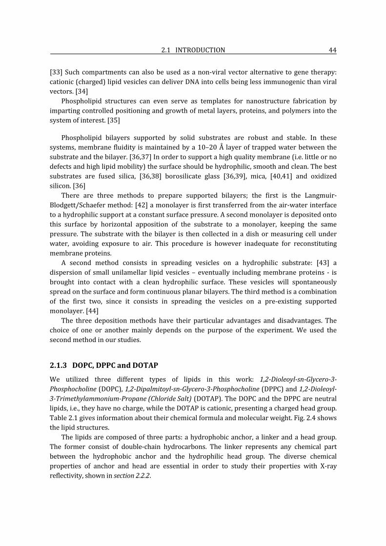
2.1 INTRODUCTION 44
[33] Such compartments can also be used as a non-viral vector alternative to gene therapy: cationic (charged) lipid vesicles can deliver DNA into cells being less immunogenic than viral vectors. [34]
Phospholipid structures can even serve as templates for nanostructure fabrication by imparting controlled positioning and growth of metal layers, proteins, and polymers into the system of interest. [35]
Phospholipid bilayers supported by solid substrates are robust and stable. In these systems, membrane fluidity is maintained by a 10–20 Å layer of trapped water between the substrate and the bilayer. [36,37] In order to support a high quality membrane (i.e. little or no defects and high lipid mobility) the surface should be hydrophilic, smooth and clean. The best substrates are fused silica, [36,38] borosilicate glass [36,39], mica, [40,41] and oxidized silicon. [36]
There are three methods to prepare supported bilayers; the first is the Langmuir-Blodgett/Schaefer method: [42] a monolayer is first transferred from the air-water interface to a hydrophilic support at a constant surface pressure. A second monolayer is deposited onto this surface by horizontal apposition of the substrate to a monolayer, keeping the same pressure. The substrate with the bilayer is then collected in a dish or measuring cell under water, avoiding exposure to air. This procedure is however inadequate for reconstituting membrane proteins.
A second method consists in spreading vesicles on a hydrophilic substrate: [43] a dispersion of small unilamellar lipid vesicles – eventually including membrane proteins - is brought into contact with a clean hydrophilic surface. These vesicles will spontaneously spread on the surface and form continuous planar bilayers. The third method is a combination of the first two, since it consists in spreading the vesicles on a pre-existing supported monolayer. [44]
The three deposition methods have their particular advantages and disadvantages. The choice of one or another mainly depends on the purpose of the experiment. We used the second method in our studies.
2.1.3 DOPC, DPPC and DOTAP
We utilized three different types of lipids in this work: 1,2-Dioleoyl-sn-Glycero-3-Phosphocholine (DOPC), 1,2-Dipalmitoyl-sn-Glycero-3-Phosphocholine (DPPC) and 1,2-Dioleoyl-3-Trimethylammonium-Propane (Chloride Salt) (DOTAP). The DOPC and the DPPC are neutral lipids, i.e., they have no charge, while the DOTAP is cationic, presenting a charged head group. Table 2.1 gives information about their chemical formula and molecular weight. Fig. 2.4 shows the lipid structures.
The lipids are composed of three parts: a hydrophobic anchor, a linker and a head group. The former consist of double-chain hydrocarbons. The linker represents any chemical part between the hydrophobic anchor and the hydrophilic head group. The diverse chemical properties of anchor and head are essential in order to study their properties with X-ray reflectivity, shown in section 2.2.2.

2.1 INTRODUCTION 45
LIPID FORMULA M. W. DOPC C44H84NO8P 786.1 DPPC C40H80NO8P 734.0
DOTAP C42H80NO4Cl 698.5
Table 2.1. Chemical formulas and molecular weights of the lipids used in this thesis work
Fig. 2.4. A. and B. Structure of the DOPC. C. and D. Structure of the DPPC. E. and F. Structure of the DOTAP. Illustrations from Avanti Polar Lipid.

2.2 INVESTIGATION OF ORDER AND CLUSTERS IN LIPID MULTIBILAYERS 46
2.2 Investigation of order and clusters in lipid multibilayers
2.2.1 Sample preparation
DOPC and DOTAP were bought from Avanti Polar Lipids. The single lipids were dissolved in chloroform at a concentration of 5 mg/ml. For the X-ray measurements, the resulting solution was immediately deposited on silicon substrates by spin-coating: approximately 10 ml of solution per mm2 was pipetted onto the surface; samples were then accelerated to rotation at 3000 rpm for 60 seconds: the solvent evaporated and a well-defined number of bilayers nucleated at the substrate surface. [45] The wafers were preliminary treated with chemical etching: silicon substrates were alternatively dipped in basic HF and HNO3 solution, following the method described elsewhere. [46] This procedure ensured a hydrogen-terminated oxide-free surface. The samples were put in vacuum overnight.
For IR-SNOM measurements, the DOPC was first dissolved in chloroform and then removed via rotary evaporation at 35 °C, leaving a thin lipid film that was later placed under vacuum for 24 hours to remove all traces of solvent. The lipid was then suspended in deionized water at 45 °C until the film was hydrated and vortex mixed to achieve an emulsion. Finally, the solution was sonicated for 30 minutes to ensure vesicles formation. The resulting solution was deposited on silicon (100) substrates by pipetting.
2.2.2 X-ray reflectivity and diffuse scattering lipid bilayer structural properties
In this section we present a quantitative specular and diffuse reflectivity study of multilamellar phospholipid membranes deposited on a solid substrate. Measurements were carried out at the Hasylab D4 beamline of the Desy synchrotron facility in Hamburg, Germany.
X-ray reflectivity is widely used in basic research and material science due to its unique ability to study the structure and the organization of materials, since it determines the electron density profile and the roughness of the interfaces. [47]
In the specific case of solid-supported lipid bilayers, this technique has been employed for a long time to investigate detailed bilayer structural parameters, [48] as well as macromolecular self-assembly, fluctuation and interaction parameters. [49]
The organization of the neutral lipid DOPC and the cationic lipid DOTAP multibilayers deposited on silicon (100) substrates was studied at the incident-beam energy of 21 keV in order to limit the radiation damage. [50] Despite the highly brilliant beam, we did not observe any variation on the measured signal, implying that no or negligible radiation damage was induced in the sample even after several hours of exposure time. The 4 mm by 4 mm sample was mounted horizontally.
The reflected intensity was measured as a function of the incident angle under specular conditions (exit angle ). Thus, the momentum transfer of the elastic scattering q was always along ( ), with the z axis parallel to the sample normal direction (number 1 in Fig. 2.5 A).
Rocking curves were measured at the first Bragg peak of the reflectivity spectra: the value was fixed and a scan in was performed. A representative acquisition is shown in Fig. 2.5 B. The sharp peak correspond to the specular component while the broad lower part to

2.2 INVESTIGATION OF ORDER AND CLUSTERS IN LIPID MULTIBILAYERS 47
the diffuse scattering component. The two lateral peaks, obtained at the critical angle, are called Yoneda wings and set a limit to the accessible space.
Fig. 2.5. A. Sketch of the accessible reciprocal space with the specular axis and the area of reciprocal space probed by non specular scattering. Number 1 indicates the scan performed under specular conditions ( ). Number 2 represent the offset scan, i.e., a reflectivity scan performed with an offset of 0.05° in order to measure the diffuse background. Number 3 is the rocking scan measured at the Bragg peak. B. Representative Rocking curve performed at the first Bragg peak of the reflectivity curve.
In order to obtain the true reflectivity signal, the diffuse (nonspecular) scattering has to be subtracted. An offset scan (indicated by number 2 in Fig. 2.5 A), corresponding to a reflectivity scan with an intentional offset , was thus performed. The offset angle choice was based on the specular rocking scan width: approximately three times the FWHM was set as the offset angle and the diffuse background was acquired with .
Fig. 2.6 A shows the reflectivity curve (red) of pure DOPC in lamellar phase, plotted as a function of the moment transfer , after an illumination correction, taking into account the variation of incident photons, and the subtraction of the offset scan. In the data, typical features of single-interface reflectivity – such as the region of total external reflection at small
– can be recognized. Moreover, the oscillations and Bragg peaks are typical of multilamellar systems. [49]
The black solid curve correspond to the best fit, performed on the first order Kiessig oscillation and Bragg peak using the Parratt model described in Chapter 1. A density profile is derived from this calculation and shown in panel B of Fig. 2.6. The air and bulk are indicated by an horizontal line with a constant value respectively equal to 0 and . The multilamellar stack of bilayers is described by the oscillatory profile, reflecting the density change between the head and tail groups. This profile also provides information about the number of layers composing the film, their dimension as well as the multibilayer total thickness.
The data fit show the presence of highly ordered multibilayers in the film of DOPC. Each bilayer of the neutral lipid has an average thickness of 41.7 Å, in good agreement with previous results achieved with X-ray and neutron reflectivity measurements. [8]

2.2 INVESTIGATION OF ORDER AND CLUSTERS IN LIPID MULTIBILAYERS 48
Fig. 2.6. A. Specular reflectivity curve of solid-supported DOPC multibilayer (in red) and its best fit (in black) using the Parratt model. B. Electron density profile across the multilamellar film.
Experimentally, a reflectivity curve with a Bragg peak and Kiessig fringes indicates an ordered film and a well-defined number of bilayers, but the sample may still exhibit a defect structure on various length scales.
The presence of domains at cell membranes can give rise to biologically important properties; for instance, the electrostatic interaction between lipids, as well as charged extracellular macromolecules and phospholipid headgroups, can induce lipid phase separation and lateral demixing under appropriate conditions, yielding the formation of segregated domains, the nucleation of transient pore and raft domains. [51] These nonhomogeneous features can be traced by X-ray diffuse scattering, which gives access to the lateral film structure on the mesoscale between a few nanometers and several micrometers.
Fig. 2.7. In red: rocking curve measured around the first Bragg peak of the DOPC reflectivity curve (Fig. 2.6 A). In black: combination of two Lorentzian best fit of the diffuse (solid line) and specular scattering (dashed line).
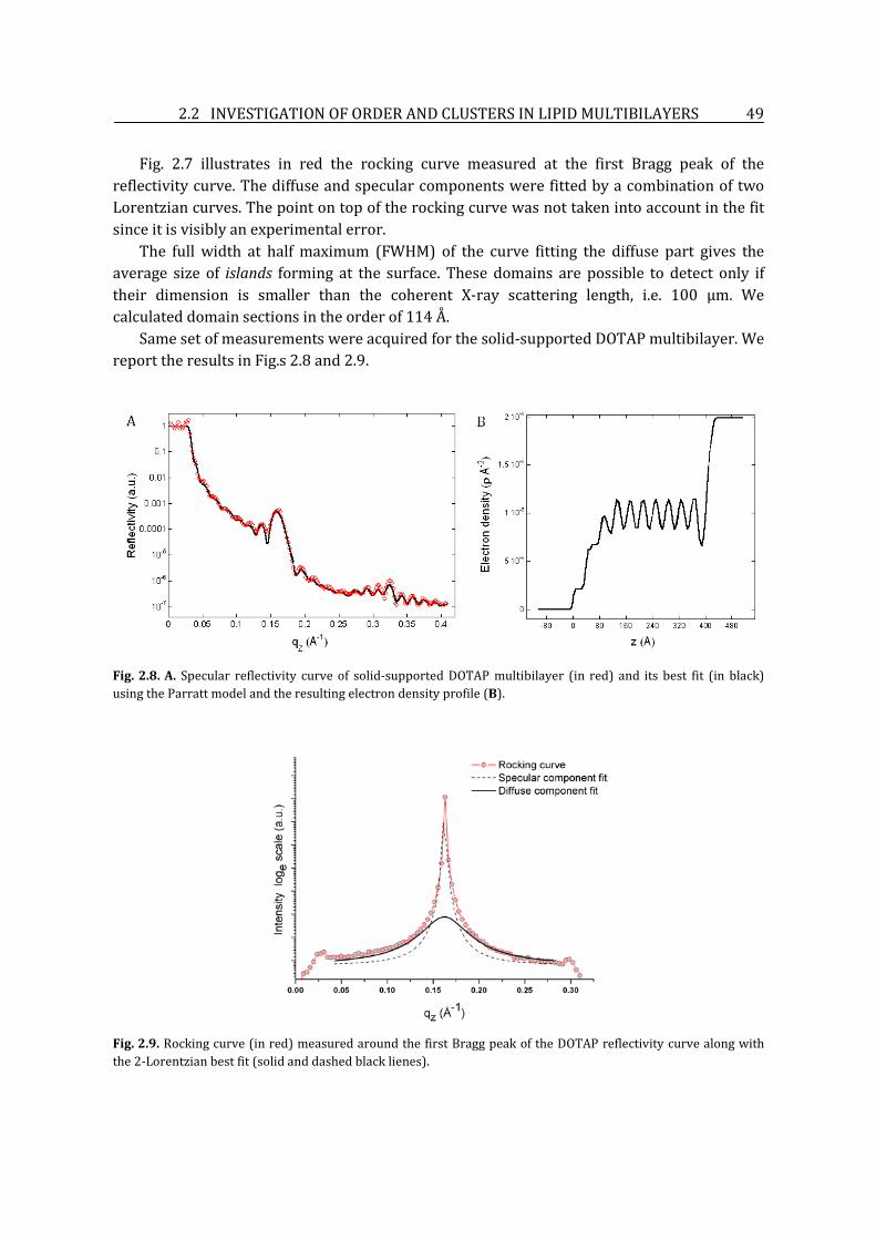
2.2 INVESTIGATION OF ORDER AND CLUSTERS IN LIPID MULTIBILAYERS 49
Fig. 2.7 illustrates in red the rocking curve measured at the first Bragg peak of the reflectivity curve. The diffuse and specular components were fitted by a combination of two Lorentzian curves. The point on top of the rocking curve was not taken into account in the fit since it is visibly an experimental error.
The full width at half maximum (FWHM) of the curve fitting the diffuse part gives the average size of islands forming at the surface. These domains are possible to detect only if their dimension is smaller than the coherent X-ray scattering length, i.e. 100 µm. We calculated domain sections in the order of 114 Å.
Same set of measurements were acquired for the solid-supported DOTAP multibilayer. We report the results in Fig.s 2.8 and 2.9.
Fig. 2.8. A. Specular reflectivity curve of solid-supported DOTAP multibilayer (in red) and its best fit (in black) using the Parratt model and the resulting electron density profile (B).
Fig. 2.9. Rocking curve (in red) measured around the first Bragg peak of the DOTAP reflectivity curve along with the 2-Lorentzian best fit (solid and dashed black lienes).

2.2 INVESTIGATION OF ORDER AND CLUSTERS IN LIPID MULTIBILAYERS 50
The cationic lipid single bilayer thickness is 38.6 Å, thinner than the DOPC bilayer. This result is in accordance with the lipid chemical structure and with X-ray and neutron reflectivity measurements. [8] From the in-plane scan analysis we extrapolated the island sections to be approximately ~ 143 Å wide.
Table 2.2 summarizes the reflectivity and diffuse scattering results performed on the two samples.
Sample Bilayer thickness Domain size DOPC 42 ± 1 Å ~ 114 Å
DOTAP 39 ± 1 Å ~ 143 Å
Table 2.2. Summarized results from X-ray specular reflectivity and diffuse scattering by solid-supported multibilayers.
Both neutral DOPC and cationic DOTAP exhibit highly ordered multibilayers along the z-direction and small in-plane (x-y) structures. In particular, the neutral lipid displays more than 20% smaller islands than the cationic one, leading us to the hypothesis that the DOTAP, as a charged lipid, has a slightly stronger tendency to form big surface domains.
2.2.3 IR-SNOM localizes membrane domains
Due to its surface sensitivity and high spatial resolution, scanning near-field optical microscopy has a significant potential to study the lateral organization of membrane domains and clusters. Such properties are crucial for possible applications in the biotechnology field, for example, with biosensors, and in medicine, with gene therapy.
Fig. 2.10. A. Orientation of a lipid bilayer along z-axis. B. Schematic of the nonhomogeneity of a lipid multibilayer surface. Drawing indicates that lipid multibilayers are oriented along the z direction and locally ordered in the plane, with an average cluster diameter of 60 Å. This value has been calculated from X-ray reflectivity, shown in section 2.1.2.
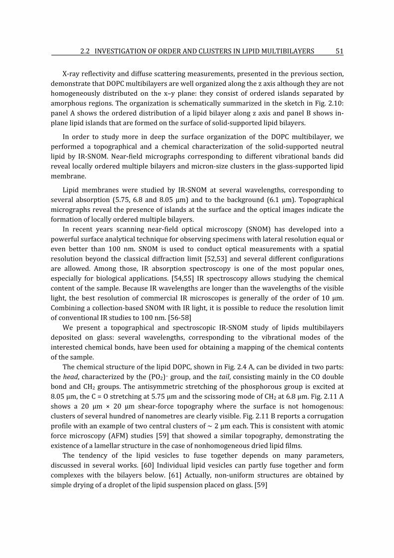
2.2 INVESTIGATION OF ORDER AND CLUSTERS IN LIPID MULTIBILAYERS 51
X-ray reflectivity and diffuse scattering measurements, presented in the previous section, demonstrate that DOPC multibilayers are well organized along the z axis although they are not homogeneously distributed on the x–y plane: they consist of ordered islands separated by amorphous regions. The organization is schematically summarized in the sketch in Fig. 2.10: panel A shows the ordered distribution of a lipid bilayer along z axis and panel B shows in-plane lipid islands that are formed on the surface of solid-supported lipid bilayers.
In order to study more in deep the surface organization of the DOPC multibilayer, we performed a topographical and a chemical characterization of the solid-supported neutral lipid by IR-SNOM. Near-field micrographs corresponding to different vibrational bands did reveal locally ordered multiple bilayers and micron-size clusters in the glass-supported lipid membrane.
Lipid membranes were studied by IR-SNOM at several wavelengths, corresponding to several absorption (5.75, 6.8 and 8.05 µm) and to the background (6.1 µm). Topographical micrographs reveal the presence of islands at the surface and the optical images indicate the formation of locally ordered multiple bilayers.
In recent years scanning near-field optical microscopy (SNOM) has developed into a powerful surface analytical technique for observing specimens with lateral resolution equal or even better than 100 nm. SNOM is used to conduct optical measurements with a spatial resolution beyond the classical diffraction limit [52,53] and several different configurations are allowed. Among those, IR absorption spectroscopy is one of the most popular ones, especially for biological applications. [54,55] IR spectroscopy allows studying the chemical content of the sample. Because IR wavelengths are longer than the wavelengths of the visible light, the best resolution of commercial IR microscopes is generally of the order of 10 μm. Combining a collection-based SNOM with IR light, it is possible to reduce the resolution limit of conventional IR studies to 100 nm. [56-58]
We present a topographical and spectroscopic IR-SNOM study of lipids multibilayers deposited on glass: several wavelengths, corresponding to the vibrational modes of the interested chemical bonds, have been used for obtaining a mapping of the chemical contents of the sample.
The chemical structure of the lipid DOPC, shown in Fig. 2.4 A, can be divided in two parts: the head, characterized by the (PO2)− group, and the tail, consisting mainly in the CO double bond and CH2 groups. The antisymmetric stretching of the phosphorous group is excited at 8.05 μm, the C = O stretching at 5.75 μm and the scissoring mode of CH2 at 6.8 μm. Fig. 2.11 A shows a 20 μm × 20 μm shear-force topography where the surface is not homogenous: clusters of several hundred of nanometres are clearly visible. Fig. 2.11 B reports a corrugation profile with an example of two central clusters of ∼ 2 μm each. This is consistent with atomic force microscopy (AFM) studies [59] that showed a similar topography, demonstrating the existence of a lamellar structure in the case of nonhomogeneous dried lipid films.
The tendency of the lipid vesicles to fuse together depends on many parameters, discussed in several works. [60] Individual lipid vesicles can partly fuse together and form complexes with the bilayers below. [61] Actually, non-uniform structures are obtained by simple drying of a droplet of the lipid suspension placed on glass. [59]

2.2 INVESTIGATION OF ORDER AND CLUSTERS IN LIPID MULTIBILAYERS 52
Structural properties of the model membrane DOPC are well known in literature. [62] The surface of lipid films has been investigated with AFM, [63] demonstrating the existence of a lamellar structure in the case of inhomogeneous dried lipid films.
Fig. 2.11. A. 20 μm × 20 μm topographical (shear-force) micrograph of solid-supported neutral lipid. B. Corrugation profile of the section indicated on the topographical micrograph.
In order to map the chemical distribution of the lipids, the free electron laser (FEL) beam was tuned at four specific wavelengths (shown at the bottom of Fig. 2.12): λ = 5.75, 6.1, 6.8 and 8.05 μm. The spatial distribution of these is shown by the darkest spots in the optical micrographs A, B, C and D of Fig. 2.12. The intensity of each pixel was normalized by the corresponding measured FEL intensity; all images were normalized to have the same dynamic range.
Fig. 2.12. FTIR microscopy spectrum of the solid-supported neutral lipid DOPC (bottom). Chemical micrographs A, B, C and D have been taken by tuning the Free Electron Laser at the wavelengths 5.75, 6.1, 6.8 and 8.05 μm.

2.2 INVESTIGATION OF ORDER AND CLUSTERS IN LIPID MULTIBILAYERS 53
The micrographs (Fig. 2.12 panel A, C and D) show similar absorption patterns: tail and head are aligned in the z direction. We can assume that islands of lamellar-structured bilayers are formed, even though these clusters are not fused together to form a flat surface. These results are supported by the X-ray reflectivity data shown in the previous section.
The optical images for absorption-peak wavelengths are not affected by topographic artifacts. This point was verified by taking the structureless image of Fig. 2.12 B at 6.1 μm, where only background noise is present with no absorption from DOPC.
Without dynamic range normalization the absorption intensity revealed by each image tracks the strength of the corresponding peak. Fig. 2.13 shows the raw chemical maps acquired at λ = 5.75, 6.1, 6.8 and 8.05 μm before the normalization. The absorption values are calculated for a specific area – delineated by the white squares in Fig. 2.13 – as well as for the whole image. The values are indicated in Fig. 2.13 E with red dots and reflect the same behaviour of the Fourier transform infrared (FTIR) spectrum peaks, pictured in the same panel. Therefore, the features of Fig. 2.12 A, C and D can be safely interpreted as being due to absorption, whereas the structures of micrograph 2.12 B can be considered only background signal, that is, 10% of the value of the other micrographs.
Fig. 2.13 A, B, C, D. Chemical mapping of the DOPC at the wavelengths 8.05, 6.8, 5.75, and 6.1 µm. E. Fourier transform infrared spectrum of the DOPC. Red circles superimposed to the spectrum correspond to the collected SNOM absorption intensity in the region delimited by a square in panels A, B, C and D.
This quantitative study proves that infrared SNOM does not only localize chemical bonds but also provides real optical signal and can measure point-by-point absorption intensity, giving information about the chemical contents relative concentration.

LIPID-ALAMETHYCIN COMPLEX CHARACTERIZATION 54
2.3 Lipid-Alamethycin complex characterization
Many functions that are crucial to cellular life are carried out by membrane proteins that are bound to or embedded in lipid bilayers. It is still difficult to determine the structure of membrane proteins by X-ray crystallography, electron crystallography or NMR spectroscopy. Nevertheless, the ability to understand certain aspects of the membrane proteins function, such as structural changes in response to physiological stimulus, may be more useful in some instances.
Membrane proteins are classified in two groups according to how tightly bound they are with the membranes. Integral proteins are associated to membranes by hydrophobic forces and can only be separated by treatment with agents that disrupt membranes. Peripheral proteins can be dissociated from membranes leaving the membrane intact.
Here we report a structural characterization of the lipid-protein system DPPC-alamethicin carried out using the energy dispersive X-ray diffractometer described in Chapter 1.
2.3.1 Alamethicin
Alamethicin is a 20-amino acid antimicrobial pore-forming peptide, produced by the fungus Trichoderma viride. [64] Fig. 2.14 shows the chemical formula of the peptide and the filamentous fungus Trichoderma.
Fig. 2.14. Chemical formula of the antimicrobial peptide alamethicin (left). On the right, the Trichoderma viride fungus. Illustration from http://www.doctorfungus.org.
The biological activities of antimicrobial membrane-active peptides are determined largely by their interactions with the phospholipid bilayer comprising the plasma membrane and by the mutual structural effects induced within the peptide and lipid molecules. [65,66]
Numerous studies have shown that membrane environments significantly affect the structural properties and functionality of membrane-active peptides. [67] Therefore, elucidating the dynamical and structural characteristics of the peptide incorporation within lipid assemblies is highly important for understanding the action mechanism and biological effects. [68]
The alamethicin exhibits a very high affinity to phospholipid bilayer. [69,70] The overall amphipathic character of alamethicin is due to the distribution of polar and nonpolar amino

LIPID-ALAMETHYCIN COMPLEX CHARACTERIZATION 55
acid residues between the lateral sides of the helix. The peptide has been studied using varied model membranes and is believed to form voltage-gate ion channels in lipid membranes according to the barrel-stave model, i.e. the trans-membrane pore consists in a cylindrical array of parallel peptide helices with a water-filled central lumen (Fig. 2.15). [71-74] Previous studies have also employed Langmuir monolayers for analysis of alamethicin association with lipid assemblies. [75-77] Pore formation processes induced by alamethicin were recently investigated in a two-dimentional phospholipid/water interface. [78,79]
Precise estimate of pore size was carried out by X-ray and neutron in-plane scattering that directly measured the internal and the external pore diameters. [74,80,81]
Fig. 2.15. A. The α-helical conformation of alamethicin with its hydrophobic and hydrophilic sides of the helix. B, C. Sketch of the interaction model between alamethicin peptides and lipid bilayers. B. Surace state of alamethicin peptides: the hydrophobic surface groups are anchored to the hydrophobic core of the bilayer. C. Barrel-stave model. Illustration from [81].
2.3.2 Lipid-peptide sample preparation
Alamethicin was purchased from Sigma–Aldrich Chemical (St. Louis, MO). The Sigma product is a mixture of components, principally alamethicin I (85% by high-performance liquid chromatography) and alamethicin II (12%), which differ by one amino acid. Different molar ratios of the DPPC/alameticin mixtures were first dissolved in a 1:1 trifluoroethanol-chloroform solvent and then uniformly deposited onto silicon substrates.
The silicon surfaces were previously washed thoroughly using 2-propanol and 1,1,1-trichloroethane in order to remove hydrophilic and hydrophobic contaminants. A nitrogen flux was finally used to remove any trace of solvent.
After deposition, the solvent evaporated leaving a smooth film, kept under vacuum for 24 h. Last, the film was hydrated with saturated water vapour and incubated for another 24 h. Our samples were prepared at lipid/peptide (L/P) molar ratios of 1, 10, 20, 30, 40, 60, 80, 160 and 320. In some cases it is more convenient to consider the inverse ratio P/L instead. The corresponding values become: 1, 0.100, 0.050, 0.033, 0.025, 0.017, 0.012, 0.006 and 0.003.
Samples were kept inside a humidity–temperature controlled chamber. We performed EDXD measurements at 50% relative humidity (RH), at constant room temperature (20°C). In

LIPID-ALAMETHYCIN COMPLEX CHARACTERIZATION 56
these conditions, the DPPC is in the fluid Lα phase. Moreover, the DPPC was also studied at 100% of relative humidity. The full hydration was achieved by keeping the sample in a chamber at H.R. 100 % for 12 hours before performing measurements.
2.3.3 DPPC-Alamethicin interaction detected by EDXD
Water is the bathing medium of most biological assemblies. Therefore it is of great importance to understand how water molecules are trapped in biological assemblies interfaces. [81] Water molecules, if present as an external medium, govern the aggregation mode of phospholipid molecules, due to the hydrophobic effect by which their apolar parts (the fatty chains) are shielded from a contact with water for minimizing the overall free energy. Considering their small size, water molecules can occupy the smallest free-volumes within lipid-peptide assemblies and, therefore, induce important effects on their conformation.
The energy dispersive X-ray diffraction spectra were collected at . During the experiments, the hydration rate was monitored inside the diffractometer chamber and only negligible variations ( ) were recorded. The Bragg peaks were fitted with Gaussian curves: their mean q value was used in the equation to obtain the bilayer thickness. Data reproducibility was tested by collecting spectra on different points of the sample.
Fig. 2.16. A. First order Bragg peaks of a DPPC lipid film deposited on a silicon support exposed at RH 50% and at RH 100%. Spectra are displayed in the reciprocal space. B. Complete spectra of partially and fully hydrated sample: three Bragg peak orders are visible for the DPPC at 100% R.H.
The diffraction spectra of partially hydrated (R.H. 50%) and fully hydrated (R.H. 100%) single DPPC lipid multibilayers are shown in Fig. 2.16 A. After the 12-hours hydration process, during measurements the relative humidity was kept at 100% by putting the DPPC sample inside a cell – built with beryllium windows, transparent to X-rays – that ensured a saturated water vapour.
The thicknesses of the partially and fully hydrated bilayers are respectively 62.5 ± 1.0 Å and 65.8 ± 1.0 Å. Without the presence of peptides, the bilayers tend to swallow and grow in thickness with hydration. This trend was already reported in previous studies. [8]

LIPID-ALAMETHYCIN COMPLEX CHARACTERIZATION 57
It is well known [82,83] that the water molecules, added during the hydration process, insert between the bilayers and help the stabilization process. This was verified in our measurements on the DPPC at R.H. 100% by the presence of second and third order Bragg peak, visible in Fig. 2.16 B. Notice that this order is not displayed by the same sample at R.H. 50%. Water molecules play therefore a critical role in the assembling stability of lipid bilayers.
The DPPC-alamethicin bilayer thicknesses (d) are reported in Table 2.3. The values were derived from the first order Bragg peak for samples studied at 50% relative humidity.
Sample d±Δd (Å) - RH 50% DPPC 62.5±1 L/P=320 P/L=0.0031 62.0±1 L/P=160 P/L=0.0062 61.6±1 L/P=80 P/L=0.0125 59.9±1 L/P=60 P/L=0.0167 57.7±1 L/P=40 P/L=0.0250 56.5±1 L/P=30 P/L=0.0333 57.6±1 L/P=20 P/L=0.0500 60.0±1 L/P=10 P/L=0.1000 60.8±1 L/P=1 P/L=1 N/A
Table 2.3. d parameter of DPPC and DPPC/Alamethicin samples at different L/P ratios at 50% R.H.
Fig. 2.17. First order Bragg peaks of DPPC/alameticin complexes at different P/L ratios deposited on a silicon support at RH 50%. A. The thinning effect is displayed: it reaches a turning point at P/L=0.025. B. A thickening effect is detected for P/L ratios higher than 0.025. Spectra are displayed in the reciprocal space.

LIPID-ALAMETHYCIN COMPLEX CHARACTERIZATION 58
Fig. 2.18. Zoom on the weak scarcely defined Bragg peak of the complex DPPC/alameticin diffraction spectra at a concentration ratio equal to 1.
In fact, inclusions of alamethicin modify the structure of the bilayer by perturbating the configuration of the lipid chain and the so-called “hydrophobic mismatch” occurs: the peptide hydrophobic part is shorter than that of the host membrane, leading to bilayer compression/expansion and peptide tilt. As the peptide concentration increases, the repulsive interaction between alamethicin molecules can lead to interface disorder and split the membrane in parts with different bilayer thickness, until a certain point, when the pores overcome the energy barrier and are forced together. [84]
Let us define as the variation between the lipid DPPC bilayer thickness and the dimension of the alamethicin/DPPC complex :
(2.1)
The thinning effect, demonstrated by our measurements, is proportional to the increase of the lipid membrane area - up to the critical value (turning point):
(2.2)
In this relation is the membrane area, is the membrane area increase; is the lipid area increase caused by one lipid and is the cross section area per lipid; is the peptide-lipid ratio. [85]
The variation normalized by the DPPC bilayer thickness is plotted as a function of the P/L ratio in Fig. 2.19. The point distribution shows a linear trend in first approximation. From the fit (solid line) it is possible to extrapolate the angular coefficient of Eq. 2.2. and thus the value , which is in agreement with the alamethicin cross section area studied by Lee et al. [86]

LIPID-ALAMETHYCIN COMPLEX CHARACTERIZATION 59
Fig. 2.19. variation as a function of the P/L ratio for partially hydrated systems. Solid line corresponds to the best linear fit.
A molecular understanding of the interaction of peptides and proteins with lipid bilayers requires experimental knowledge of the structure of the membrane bilayer, the transbilayer location of bound peptides, the structures the peptides adopt, and the changes that occur in the bilayer structure as a result of partitioning. Because cellular membranes must be in a fluid state for normal cell function, it is the structure of fluid (Lα-phase) bilayers that is relevant to understanding the interactions of peptides in molecular detail.
Since multilamellar bilayers deposited on surfaces are highly periodic along the bilayer normal it was possible to study the structure of the DPPC solid-supported membrane with energy dispersive X-ray diffraction and demonstrate the critical role of water molecules in the membrane ordering and assembling process, by comparing the diffraction spectra of the same sample before and after full hydration.
The interaction of the membrane with the antimicrobial membrane-active peptide alamethicin was investigated at different lipid/peptide concentrations, detecting strong structural changes in the bilayer conformation. The “hydrophobic mismatch” between lipids and peptide was demonstrated in the 2-phase thinning-thickening behaviour of the bilayer as the peptide concentration increased: the shorter peptide hydrophobic part induces a compression in the host membrane until a certain point, after which the bilayer thickness start expanding again. From the linear thinning trend we extrapolated the alamethicin cross-section area.
Understanding the DPPC/alamethicin complex behaviour at 100% R.H., simulating in-vivo conditions, is of great relevance: the role played by water-filled alamethicin channels has still not been clarified. Measurements on the fully hydrated (100% R.H.) systems are in progress.
Moreover, we are planning to perform high resolution contact and non-contact atomic force microscopy measurements on the lipid/peptide samples at different peptide concentration in order to study the membrane structure and eventually visualize the formation of alamethycin channels at the surface.

LIPID-ALAMETHYCIN COMPLEX CHARACTERIZATION 60
Furthermore, the use of nanospectroscopy will allow a chemical characterization of the complex at nanometric level. Our aim is to localize the alamethycin on the membrane by mapping the topographical and chemical variations with Raman nanospectroscopy (discussed in Chapter 4).
References
[1] Castellana, E. T., P. S. Cremer. Surface Science Reports 61, 429–444 (2006). Sackmann, E. Science 271, 43 (1996).
[2] Voet, D., J. G Voet. Biochemistry. USA: Wiley International, 2004 [3] Generosi, J., M. Piccinini, A. Marcelli, S. Belardinelli, D. Pozzi, A. Congiu Castellano.
Infrared Physics & Technology 50, 14 (2007). [4] Braun, C. S., G. S. Jas, S. Choosakoonkriang, G. S. Koe, J. G. Smith, C. R. Middaugh. Biophys. J.
84, 1114 (2003). [5] Safinya, C. R. Curr. Opin. Struct. Biol. 11, 440 (2001). [6] Koltover, I., T. Salditt, J. O. Rädler, C. R. Safinya. Science 281, 78 (1998). [7] Radler, J. O., I. Koltover, T. Salditt, C. R. Safinya. Science 275, 810 (1997). [8] Generosi, J., C. Castellano, D. Pozzi, R. Felici, G. Fragneto, F. Natali, A. Congiu. J. Appl. Phys.
96, 6839 (2004). [9] Gershon, H., R. Ghirlando, S. B. Guttman, A. Minsky. Biochem. 32, 7143 (1993).
[10] Zuidam, N. J., Y. Barenholz. Biochim. Biophys. Acta 1368, 115 (1998). [11] Hirsch-Lerner, D., Y. Barenholz. Biochim. Biophys. Acta 1370, 17 (1998). [12] Bhattacharya, S., S. S. Mandal. Biochem. 37, 7764 (1998). [13] Xu, Y., S. W. Hui, P. Frederik, F. C. Jr Szoka. Biophys. J. 77, 341 (1999). [14] Kawaura, C., A. Noguchi, T. Furuno, M. Nakanishi. FEBS Lett. 421, 69 (1998). [15] Oberle, V., U. Bakowsky, I. S. Zuhorn, D. Hoekstra. Biophys. J. 79, 1447 (2000). [16] Sakurai, F., T. Nishioka, H. Saito, T. Baba, A. Okuda, O. Matsumoto, T. Taga, F. Yamashita, Y.
Takakura, M. Hashida. Gene Ther. 8, 677 (2001). [17] Huebner, S., B. J. Battersby, R. Grimm, G. Cevc. Biophys. J. 76, 3158 (1999). [18] Kasahara, K., Y. Sanai. Trends Glycosci. Glycotechnol. 13, 587 (2001). [19] Stoddart, A., M. L. Dykstra, B. K. Brown, W. X. Song, S. K. Pierce, F. M. Brodsky. Immunity
17, 451 (2002). [20] Qi, S. Y., J.T. Groves, A. K. Chakraborty. Proc. Natl Acad. Sci. USA 98, 6548 (2001). [21] Plant, A. L., M. Brighamburke, E. C. Petrella, D. J. Oshannessy. Anal. Biochem. 226, 342
(1995). [22] Pum, D., G. Stangl, C. Sponer, K. Riedling, P. Hudek, W. Fallmann, U. B. Sleytr.
Microelectron. Eng. 35, 297(1997). [23] Yang, T. L., S. Y. Jung, H. B. Mao, P. S. Cremer. Anal. Chem. 73, 165(2001). [24] Yang, T. L., O. K. Baryshnikova, H. B. Mao, M. A. Holden, P. S. Cremer. J. Am. Chem. Soc. 125,
4779(2003). [25] Muller, P., D. O. Rudin, H. Ti Tien, W. C. Wescott. Nature 194, 979(1962). [26] Muller, P., D.O. Rudin, H. Ti Tien, W. C. Wescott. J. Phys. Chem. 67, 534(1963). [27] Tamm, L. K., H. M. McConnell. Biophys. J. 47, 105 (1985). [28] Groves, J. T., N. Ulman, S.G. Boxer. Science 275, 651 (1997). [29] Cremer, P. S., T. L. Yang. J. Am. Chem. Soc. 121, 8130 (1999).

REFERENCES 61
[30] Groves, J. T., L. K. Mahal, C. R. Bertozzi. Langmuir 17, 5129 (2001). [31] Yang, T. L., S. Y. Jung, H. B. Mao, P. S. Cremer. Anal. Chem. 73, 165 (2001). [32] Mao, H. B., T. L. Yang, P. S. Cremer. Anal. Chem. 74, 379 (2002). [33] Karlsson, A., R. Karlsson, M. Karlsson, A. S. Cans, A. Stromberg, F. Ryttsen, O. Orwar.
Nature 409, 150 (2001). [34] Chesnoy, S., L. Huang. Annu. Rev. Biophys. Biomol. Struct. 29, 27 (2000). [35] Lvov, Y. M., R. R. Price. Colloids. Surf. B 23, 251 (2002). [36] Tamm, L. K., H. M. McConnell. Biophys. J. 47, 105 (1985). [37] Johnson, S. J., T. M. Bayerl, D. C. McDermott, G. W. Adam, A. R. Rennie, R. K. Thomas, E.
Sackmann. Biophys. J. 59, 289 (1991). [38] Lagerholm, B. C., T. E. Starr, Z. N. Volovyk, N. L. Thompson. Biochemistry 39, 2042 (2000). [39] Cremer, P. S., S. G. Boxer. J. Phys. Chem. B 103, 2554 (1999). [40] Zasadzinski, J. A. N., C. A. Helm, M. L. Longo, A. L. Weisenhorn, S. A. C. Gould, P. K. Hansma.
Biophys. J. 59, 755 (1991). [41] Egawa, H., K. Furusawa. Langmuir 15, 1660 (1999). [42] Tamm, L. K., H. M. McConnell. Biophys. J. 47, 105 (1993). [43] Brian, A., H. M. McConnell. Proceedings of the National Academy of Sciences USA 81, 6159
(1984). [44] Kalb, E., S. Frey, L. K. Tamm. Biochim. Biophys. Acta 1103, 307 (1992). [45] Pompeo, G., M. Girasole, A. Cricenti, F. Cattaruzza, A. Flamini, T. Prosperi, J. Generosi, A.
Congiu Castellano. Japanese Journal of Applied Physics 45, 2310 (2006). [46] Dufrêne, Y., G. U. Lee. Biochim. Biophys. Acta 1509, 14 (2000). [47] Tolan, M. X-ray scattering from soft-matter thin films: materials science and basic research.
Berlin: Springer, 1999. [48] Katsaras, J., V. A. Raghunathan. Lipid bilayers: Structure and Interactions. New York:
Springer, 2000. [49] Salditt, T., C. Li, A. Spaar, U. Mennicke. Eur. Phys. J. E 7, 105 (2002). [50] Salditt, T., C. Münster, J. Lu, M. Vogel, W. Fenzl, and A. Souvorov, Phys. Rev. E 60, 7285
(1999). [51] Jing, H. Y., D. H. Hong, B. D. Kwak, D. J. Choi, K. Shin, C.-J. Yu, J. W. Kim, D. Y. Noh, Y. S. Seo.
Langmuir (2009), doi: 10.1021/la802868r. [52] Pohl, D. W., W. Denk, M. Lanz. Appl. Phys. Lett. 44, 651 (1984). [53] Dunn, R. C. Chem. Rev. 99, 2891 (1999). [54] Braun, C. S., G. S. Jas, S. Choosakoonkriang, G. S. Koe, J. G Smith, C. R. Middaugh. Biophys. J.
84, 1114 (2003). [55] Vobornik, D., G. Margaritondo, J. S. Sanghera, et al. Infrared Phys. Technol. 45, 409 (2004). [56] Cricenti, A., R. Generosi, P. Perfetti, J. M. Gilligan, N. H. Tolk, C. Coluzza, G. Margaritondo.
Appl. Phys. Lett. 73, 151 (1998). [57] Cricenti, A., R. Generosi, C. Barchesi, M. Luce, M. Rinaldi. Rev. Sci.Instrum. 69, 3240
(1998). [58] Cricenti, A., Generosi, R., Luce, M. et al. (2003). Biophys. J. 85, 2705–2710. [59] Cohen, S. A., L. A. Bagatolli. Langmuir 20, 9720 (2004). [60] Reviakine, I., A. Brisson. Langmuir 16, 1806 (2000). [61] Kumar, S., J. H. Hoh. Langmuir 16, 9936 (2000). [62] Salditt,T., C. Li, A. Spaar, U. Mennicke. Phys. Rev. Lett. 79, 2582 (1997). [63] Pompeo, G., M. Girasole, A. Cricenti, F. Cattaruzza, A. Flamini, T. Prosperi, J. Generosi, A.
Congiu. Biochim. Biophys. Acta 1712, 29 (2005). [64] Meyer, P., F. Reusser, Experimentia 23, 85 (1967). [65] Shai, Y. Biochim. Biophys. Acta 1462, 55 (1999). [66] Kessel, A., N. Ben-Tal. Curr. Top. Membr. 52, 205 (2002). [67] Shai, Y. Biochim. Biophys. Acta 1462, 55 (1999).

REFERENCES 62
[68] Volinsky, R., S. Kolusheva, A. Berman, R. Jelinek. Langmuir 20, 11084 (2004). [69] Banerjee, U., S. I. Chan. Biochemistry 22, 3709 (1983). [70] North, C. L., M. Barranger-Mathys, D. S. Cafiso. Biophys. J. 69, 2392 (1995). [71] Hall, J. E., I. Vodyanov, T. M. Balasubramanian, G. R. Marshall. Biophys. J. 45, 233 (1984). [72] Sansom, M. S. Q. Rev. Biophys. 26, 365 (1993). [73] Ojcius, D. M., J. D. Young. Trends Biochem. Sci. 16, 225 (1991). [74] Yang, L., T. A. Harroun, T. M. Weiss, L. Ding, H. W. Huang. Biophys. J. 81, 1475 (2001). [75] Doty, P., J. H. Shulman. Discuss. Faraday Soc. 6, 21 (1949). [76] Colacicco, G. J. Colloid Interface Sci. 29, 345 (1969). [77] Brockman, H. Curr. Opin. Struct. Biol. 9, 438 (1999). [78] Ionov, R., A. El-Abed, A. Angelova, M. Goldmann, P. Peretti. Biophys. J. 78, 3026 (2000). [79] Ionov, R., A. El-Abed, M. Goldmann, P. Peretti. J. Phys. Chem. B 108, 8485 (2004). [80] Qian, S., W. Wang, L. Yang, H. W. Huang. Biophys. J. 94, 3512 (2008). [81] Li, C., T. Salditt. Biophys. J. 91, 3285 (2006). [82] Milhaud, J. Biochim. Biophys. Acta 1663, 19 (2004). [83] Binder, H. Eur. Biophys. J. 36, 265 (2007). [84] Constantin, D., G. Brotons, A. Jarre, C. Li, T. Salditt. Biophys. J. 92, 3978 (2007). [85] Domenici, F., D. Panichelli, A. Congiu Castellano. Colloids Surf. B: Biointerfaces (2009), doi:
10.1016/j.colsurfb.2008.11.029. [86] Lee, M., F. Chen, H. W. Huang. Biochemistry 26, 2751 (1987).

CHAPTER 3
HIPPOCAMPAL NEURON CELLS
3.1 Introduction
Although the study of the brain can be traced back as far as centuries ago, at the time of Egyptians and Greeks, neuroscience research increased significantly only in the second half of the twentieth century after revolutions in molecular biology, computational science and microscopy. Even though the understanding of how the brain works is far from being a solved issue, new tools and technologies brought great advances in the last two decades, breaking through old beliefs and enlightening some of the most intricate problems ever faced in medical science.
Fig. 3.1. Sketch of a neuron cell. While the axon is responsible for sending information from the cell body to other cells, dendrites bring information from other neurons to the cell body. Illustration from nia.nih.gov.
The human brain is an organ that represents in the adult less than 3% of the body weight. It consists of a complex network of more than hundred billions neurons and even more glial cells. Each neuron cell connects and communicates through approximate ten thousand specialized cell junctions, called synapses. [1] The pattern of synaptic connections supports all

3.1 INTRODUCTION 64
aspects of brain function, from sensory perception and movement to learning and memory. The complexity of the brain resides also in the heterogeneous nature of neurons, since they can be classified into perhaps as many as ten thousands different types. Differences in their structure, but also in their molecular content, allow the generation of very different patterns of activity responsible for brain function. Understanding the development of neuron synapses is crucial to understand the development of the nervous system abnormalities which underlie neurological and behavioural disorders.
Before the development of good microscopes, the brain was thought to work as a gland. In 1873 the Italian physician and scientist Camillo Golgi discovered a method of staining nervous tissue which would mark randomly a limited number of cells, in their entirety. This enabled him to view the paths of nerve cells in the brain for the first time. By improving this kind of staining, the Spanish histologist and physician Santiago Ramón y Cajal postulated that the nervous system was made up of billions of separate neurons and that these cells were "dynamically polarized", i.e., they received information at their cell bodies and dendrites, and transmitted it unidirectionally towards other sites via their axons. Rather than forming a continuous web, Cajal suggested that neurons communicate with each other via specialized junctions called synapses. The ability to visualize separate neurons led to the eventual acceptance of the neuron doctrine.
One of the most remarkable properties of neurons is synaptic plasticity, i.e. the ability to modulate the strength of the synaptic response. [2] It is now thought that long-lasting change in synaptic function is the cellular basis of learning and memory. [3-7] Neuroscientists focus now their studies trying to understand the learning mechanism and where our memories are stored. This chapter is dedicated to experiments specifically designed to elucidate some aspects of synapse plasticity in hippocampal neuron cells that are thought to be responsible for short and long-term memory.
3.1.1 Synapses
Synapses are specialized intercellular junctions between neurons or between neurons and other excitable cells where signals are propagated from one cell to another.
The use of electron microscopy and other similar techniques allowed to visualize the structure of synapses, especially identifying a thicker membrane, more electron-dense than other substructures, named the postsynaptic density (PSD), [8,9] responsible for the propagation of the signal.
Synapses are defined as electrical or chemical depending upon whether transmission occurs via direct propagation of the electrical stimulus in the presynaptic process or via chemical intermediate. Even though electrical synapses play a role in synchronizing neuronal activity, [10] most synapses are chemical synapses, i.e., sites of discontinuity of the neuronal network where propagation of the signal is highly regulated. At chemical synapses, the presynaptic electrical signal is converted into a secretory response, leading to the release of chemical intermediates, the neurotransmitters, into the synaptic cleft. This chemical message is then reconverted postsynaptically into an electrical signal along the dendrites (Fig. 3.2). [2,11,12]

3.1 INTRODUCTION 65
Fig. 3.2. Drawing of a chemical synapse. Synaptic vesicles release the neurotransmitters through exocytosis in the narrow synaptic cleft. The chemical signal is converted to an electrical signal in the postsynaptic neuron. Illustration from eapbiofield.wikispaces.com.
In the mammalian brain, the majority of chemical synapses are excitatory and use glutamate as neurotransmitter. However, there is a great diversity of neurotransmitters which can lead to either an excitation or an inhibition of the postsynaptic cell.
3.1.2 AMPA receptors
Most excitatory activity in the brain is mediated by two types of glutamate receptors: α-amino-3-hydroxy-5-methyl-4-isoxazole-propionic acid (AMPA) and N-methyl-D-aspartate (NMDA) receptors, clustered in the postsynaptic membrane (Fig. 3.3). These two types of receptors have very different roles in synaptic function. AMPA receptors (AMPARs) mediate most excitatory (depolarizing) currents in conditions of basal neuronal activity, and hence, they have a major influence in the strength of the synaptic response. [1,13,14] NMDA receptors (NMDARs), on the other hand, remain silent at resting membrane potential. [15]
Fig. 3.3. Schematic of the PSD organization. After AMPARs reach the synapse, they can be either recycled through a maintenance cycle or sent to degradation. The addition of AMPARs is regulated by the NMDARs. Illustration from celanphy.science.ru.nl.

3.1 INTRODUCTION 66
Although AMPARs and NMDARs reside in the same synapses in most brain regions, they reach their synaptic targets through quite different programs. In the brain, soon after birth, most excitatory synapses in the hippocampus and other brain regions contain only NMDARs, whereas the prevalence of AMPARs increases gradually over the course of postnatal development. In fact, the delivery of AMPARs into synapses is a regulated process that depends on NMDAR activation and underlies some forms of synaptic plasticity in early postnatal development [16-18] and in mature neurons. [19]
As already mentioned, synaptic plasticity is thought to underlie higher cognitive functions, such as learning and memory, and is also critical for neural development. [20] Thus, it is not surprising that alterations in synaptic plasticity have been implicated in the pathology of several neurological disorders, including schizophrenia, [21] Alzheimer disease [22] and epilepsy. [23] Consequently, elucidating the mechanisms underlying synaptic plasticity, such as the regulation of AMPAR trafficking is extremely important.
AMPARs are heterotetrameric glutamate-gated ion channels that are composed by different combinations of the four subunits GluR1-4. [24,25] They can reach synapses by two distinct pathways, depending on their subunit composition. GluR2–GluR3 oligomers are continuously delivered into synapses in a manner largely independent from synaptic activity, [26] whereas GluR1–GluR2 and GluR4-containing receptors are added into synapses in a manner dependent upon NMDAR activation. [17,27] These subunit-specific rules for trafficking have led to a model in which GluR2–GluR3 receptors continuously cycle in and out of synapses such that the total number of AMPARs at synapses is preserved (constitutive pathway), whereas GluR1–GluR2 (and GluR4) receptors are added into synapses in an activity-dependent manner during plasticity (regulated pathway). Fig. 3.3 shows a scheme of this process.
The last step in the long journey of AMPARs is their delivery into the specialized dendritic membrane that constitutes the postsynaptic terminal.
The controlled removal of AMPARs from synapses is as important as the delivery of new AMPARs for synaptic function and plasticity. Similar to the constitutive and regulated pathways for synaptic delivery, there are also constitutive and regulated pathways for the trafficking of AMPARs out of synapses.
It is now well established that the opening of NMDARs with the concomitant entry of Ca2+ ions in the postsynaptic terminal triggers both the regulated addition and removal of synaptic AMPARs. Therefore, the number of signalling pathways that need to be activated for AMPAR delivery increases during development, in agreement with the empirical observation that synaptic plasticity is more difficult to trigger later in life. [28]
By changing the amount of AMPARs, synaptic transmission can be either enhanced or depressed. These alterations can last from few milliseconds to days, weeks, or even longer. Such efficacy changes are very important for several aspects of neural function. Transient modifications have been associated with short-term adaptation to sensory inputs, changes in behavioural states and short-term memory. [29] More lasting changes have been associated with neuronal development in the immature nervous system, as described above, and with long-term memory in the mature nervous system. [30] Therefore, the more we learn about the details of receptor trafficking and synaptic plasticity, the better we will be able to identify

3.1 INTRODUCTION 67
the molecular or cellular changes triggered by a particular neural function. In fact, considering how fast this research field is moving, we may not be too far away from understanding what memories are made of.

3.2 SAMPLE PREPARATION 68
3.2 Sample preparation
It may sound trivial, but successful SNOM measurements can be performed only if the samples are well prepared. This condition applies especially when analyzing biological samples that are, per se, affected by external conditions, such as temperature, humidity and light, and by aging, since in most cases samples can damage with time.
Neuron samples were in fact prepared by our collaborators in the Cellular Neurobiology Laboratory of the EPFL with the specific aim of performing fluorescence and infrared SNOM measurements. A dedicated attention was thus given especially to:
• The labelling procedure: the use of resistant fluorophores is essential in scanning near-field optical microscopy. Even though the SNOM illumination geometry allows to shine only on the point of interest while scanning, photobleaching still affects the measurements reducing the fluorescence signal already very difficult to detect.
• The removal of all growing medium traces: a washed cleaned surface is essential since the presence, for instance, of PBS crystals avoids the correct topographical reconstruction and may give artifactual contributes to the optical and chemical signals.
3.2.1 Cell culture
Hippocampal neurons were extracted from 7-days-old P0 Sprague-Dawley rats (Charles River/Iffa Credo, L’Arbresle Cedex, France) according to Steiner et al. [31] Hippocampi were dissected in HBSS medium (Invitrogen, Carlsbad, USA) and incubated in dissociation medium - 90 mM Na2SO4, 30 mM K2SO4, 0.2 mM NaOH, 1.6 mM HEPES/KOH, 0.25 mM CaCl2, 5.8 mM MgCl2, 20 mM glucose, 6.3 mM L-cysteine (Sigma-Aldrich, Steinheim, Germany), 200 U papain (Sigma-Aldrich, Steinheim, Germany) - at pH 7.4 and 292 mOsmoles, for 30 min at 34°C. The neurons were spun at 200g for 2 min in a Beckman centrifuge and the dissociation medium was changed to a protease inhibitor solution - 90 mM Na2SO4, 30 mM K2SO4, 0.2 mM NaOH, 1.6 mM HEPES/KOH, 0.25 mM CaCl2, 5.8 mM MgCl2, 20 mM glucose, 1 mg/ml trypsin inhibitor, 1 mg/ml BSA - for 15 min incubation at RT. The cells were triturated in trituration medium (Earle’s MEM medium, Invitrogen, Carlsbad, USA, 20 mM glucose, 0.5 mM glutamine, 10% horse serum, Amimed, Basel, Switzerland) using a borosilicate glass pipette. The hippocampal neurons were plated in growth medium (Earle’s MEM medium, 20 mM glucose, 0.5 mM glutamine, 100 U/ml penicillin, 100 µg/ml streptomycin, 10% horse serum) on borosilicate glass coverslips (Marienfeld GmbH&Co.KG, Lauda-Königshofen, Germany) coated with poly-D-lysine (5 µg/ cm2, BD Biosciences, Franklin Lakes, USA) and laminin (0.7 µg/ cm2, Invitrogen, Carlsbad, USA) at a density of 12500 cells/cm2. After 2 h the growth medium was changed to Neurobasal medium/B27 (Neurobasal medium, Invitrogen, USA, 1x B27 Invitrogen, USA, 0.5 mM glutamine, 100 U/ml penicillin, 100 µg/ml streptomycin). The hippocampi were kept in culture at 37°C and 5% CO2. Three days after plating, neurons were infected with 100 µl at 1000 ng /ml p24 of the lentivirus SIN-PGK-ACP-GluR2 and then incubated further 14-21 days. [32]

3.2 SAMPLE PREPARATION 69
3.2.2 Acyl carrier protein (ACP) labeling
In biological science and medical diagnostics it is common use to add fluorophores to proteins allowing tracking and quantification. Usually, in vitro, the procedure is to let the proteins covalently bound to the dyes. Excess of fluorophores and damaged proteins are later washed away. By coupling a fluorophore to an antibody it is possible to specifically localize a protein in fixed cells or track it on the surface of a living cell. [33]
Among the revolutionary advances lately brought by genetic engineering lies a new way of tagging proteins. By modifying chemically a synthetic protein or peptide it is possible to create a small and convenient tag to attach to the desired target. One of these tags is the Acyl Carrier Protein (ACP).
Carrier proteins are small proteins composed by 70-80 amino acid residues and take part in several metabolic processes, such as fatty acid synthesis, non ribosomal peptide synthesis.
Fig. 3.4 shows how the surface receptor AMPA can be labelled with the ACP technique: the ACP, extracted by E. Coli, fused to the GluR subunit is modified by the PPTase and links covalently to to the Coenzyme A (CoA) when modified by a phosphopantethein transferase (PPTase). Details are explained in the paper by Johnsson et al. [34]
Fig. 3.4. Scheme of the ACP labelling technique. The surface AMPAR GluR subunits are fused together with the acyl carrier protein which goes through a PPTase to covalently link to the Coenzyme A and therefore to the desired label.
Neurons on 18 mm glass coverslips were incubated for 15 min at room temperature with 150 μl of PBS buffer containing MgCl2 (10 mM), 6xHis-AcpS (1 μM) and 5 µM CoA-Alexa488. After washing with PBS, the neurons were fixed in a solution with 4% paraformaldehyde, 4% sucrose in PBS for 12 min. The neurons were afterwards washed twice in PBS and stored at 4°C before being analyzed with scanning near-field optical microscopy.
3.2.3 Lentiviral production
Viral vectors are commonly used in gene therapy [35,36] to introduce into cells a new gene trascription. In our case, HIV-derived lentiviral vectors are transfected into the neuron cells. The viruses do not contain genes coding for viral proteins but for the specific tag protein, essential to make the labeling successfull. Thanks to their high transfection efficiency, these

3.2 SAMPLE PREPARATION 70
viral vectors can bring to the fluorescence staining of more than 80% of the total amount of neurons grown on the coverslip.
For the lentiviral production, 20 dishes of 9 cm2 with 3 x 10⁶ 293T cells per dish were plated. 24 h after plating the cells were transfected with the following plasmids: 13 µg per dish of pCMVΔ8.92 (Fasteris, Geneva, Switzerland), 3 mg per dish of pRSV-ReV, 3.75 µg per dish of pMD2G and 13 µg per dish of the plasmid SIN-PGK-ACP-GluR2-WHV vector. For the transfection of 20 dishes a solution was prepared with 10ml of CaCl2 0.25M and the DNA mix. A second solution of HeBS 2x (0.28 M NaCl, 0.05M HEPES, 1.5 mM Na2HPO4, pH 7.05) was prepared in a second tube and the DNA solution was adjonted slowly to the HBS 2X solution under agitation. Then 1 ml of the solution was added to each dish. The medium was changed after 6 h.
72 h after transfection the medium was collected in 30 ml tubes (Beckman) and spun at 19000 rpm and 4°C for 90 min in an ultracentrifuge. 5 µl of medium is kept and lysed in 45 µl lysis buffer (Zeptometrix Corporation, Buffalo, USA) for titration. The supernatant is removed and the pellet is resuspended in a final volume of 3 ml of PBS, 0.5% BSA for a 50X concentration. 5 µl were kept and lysed for titration. The viral titer is determined using the HIV-1 P24 elisa kit (Zeptometrix Corporation).
3.2.4 The fluorophore Alexa 488
The family of Alexa fluorophores are synthesized through sulfonation of coumarin, rhodamine, xanthenes and cyanine dyes. [37] Sulfonation makes the dyes negatively charged and hydrophilic. Alexa markers are generally more stable and brighter than other standard dyes of comparable excitation and emission. The individual family members are numbered according to their excitation maxima.
We used Alexa 488 in our experiments, since the wavelength of the excitation light utilized, i.e., the blue line of an Argon laser, is 488 nm.
When shining on the sample, the fluorophores absorbs energy: when the transition is possible, its molecules are brought to an excited electron state. When the molecule returns to the electronic ground state, fluorescence light is emitted. Together with this phenomenon, vibrational state excitation and relaxation – with consequent thermal dissipation – take place. Therefore, the reemitted light has longer wavelength. The maximum emission of the Alexa 488 occurs around 515 nm.

3.3 AMPARS MAPPING WITH FLUORESCENCE SNOM 71
3.3 AMPARs mapping with fluorescence SNOM
3.3.1. Why scanning near-field optical microscopy?
Scanning near-field optical microscopy (SNOM) yields subwavelength optical information, overcoming the Abbé-Rayleigh diffraction limit, [38,39] together with shear-force (topographic) images. [40,41]
With a conventional optical microscope, diffraction limits the resolution to approximately half of the wavelength used, which can be translated in a 250-300 nm spatial resolution for visible light. Therefore, two fluorescently-labelled-microstructures can be resolved only when the distance in between them is about 250-300 nm. SNOM beats the diffraction limit thus reaching high lateral resolution. The distance between sample and tip, the aperture of the tip and the scanning step are smaller than , thus reaching less than 100 nm resolution for visible light.
Apart for the great resolution possible to achieve, even on thick samples such as cells, SNOM is particularly suited to study biological specimens because it can perform imaging without damaging the sample, due to its shear-force feedback mechanism used to position the tip in close proximity to the surface.
Moreover, illumination mode SNOM is preferable, if not necessary, when investigating samples that are light sensitive. For our specific case, biological fluorescence spectroscopy requires the sample to be illuminated by the probe for two fundamental reasons:
• The probability of creating a fluorescence photon with an incident excitation photon is linearly proportional to the chromophore scattering section and inversely proportional to the area of the excitation beam. [42] SNOM decreases the excitation beam cross section, thus increasing the fluorescence efficiency per incident photon. Because illumination mode operation minimizes background signal interference – including Rayleigh scattering or even Raman scattering that might originate anywhere along the optical path, e.g., in the fiber, the sample, the substrate, etc. – problem caused by these effects are easier to correct.
• Illumination mode SNOM also reduces the effect of photodamage to light-sensitive samples. [43] Molecular photobleaching can occur after prolonged light exposure, so only molecules within the probe field of view should be excited. With illumination SNOM, only the sample region under immediate investigation is illuminated. In contrast, by using collection mode SNOM a large region of the sample is illuminated, while only a region directly beneath the aperture is imaged.
With fluorescence SNOM we simultaneously obtain topographical, fluorescence and transmission micrographs of the sample. These topographic micrographs are extremely important for the interpretation of SNOM images, specifically to link optical features with topographic ones. Fig. 3.5 is an example. The shear-force image (panel A) is acquired in the zero-crossing mode: [44] each data point is measured in an asynchronous way, collecting the signal only when the shear-force value equals the reference, thus eliminating the error-signal. This method guarantees a constant probe-sample distance for each pixel, ensuring artefact-free optical micrographs, simultaneously obtained during the scan. Panel B shows the

3.3 AMPARS MAPPING WITH FLUORESCENCE SNOM 72
fluorescence record of the same area. Brightest spots correspond to highest fluorescence emission. Transmission of light through the sample is illustrated in panel C: darkest regions correspond to higher absorption by the specimens.
Fig. 3.5. Topography, fluorescence map and transmission image of a neuron cell. The green circle enhances the highest part in panel A, the brightest fluorescence in panel B and the most absorbing, i.e., densest, spot in panel C. The wavelength of the excitation light is 488 nm.
3.3.2 AMPA trafficking
AMPAR trafficking is an important issue in neurobiology, extensively studied with a broad spectrum of experimental techniques. [45,46] These efforts notwithstanding, the key questions remain rather controversial. Here we show that F-SNOM can contribute to the solution of this important problem by detecting the surface distribution of AMPAR on the neuron membrane and providing evidence for a diffusion pathway.
Fig. 3.6. A. 29 µm x 29 µm 3D AFM topography of a neuron cell. B. Confocal microscopy image of a hippocampal neuron cells. Bright spots correspond to the fluorescence emission by the Alexa 488 dyes marking the GluR1 subunits of the AMPA receptors.
We studied hippocampal neurons from 7-days-old rats, still in the postnatal brain development stage. Preliminary atomic force microscopy measurements were performed on the samples. Fig. 3.6 A shows a three-dimensional non-contact AFM image of a neuron cell.

3.3 AMPARS MAPPING WITH FLUORESCENCE SNOM 73
AMPAR GluR2 subunits were marked with the Alexa 488 fluorophore. Fig. 3.6 B shows a conventional confocal microscopy image of a neuron cell with its dendrites. Bright spots correspond to receptor clusters. Despite the ease of use and the sectioning capabilities, confocal microscopy is affected by diffraction and has therefore a low optical resolution.
Differently from what confocal images show, AFM studies confirm the presence of an intricate neurites network covering like a carpet the surface of the sample, clearly visible in Fig. 3.7.
Fig. 3.7. Representative 20 µm x 20 µm atomic force microscopy image of the intricate network of neurites present on the glass surface of the analyzed samples.
Fig. 3.8. A. 25 μm x 25 μm topography of a neuron body. The dashed circle indicates the highest region. B. Transmission image at 488 nm. The intensities are in arbitrary unit. The dashed circle indicates the maximum absorption. C. Alexa 488 fluorescence map. The dashed circle indicates the maximum emission. The intensity is in arbitrary unit. D, E, F. Profile images of corresponding white lines drawn respectively in panel A, B and C.

3.3 AMPARS MAPPING WITH FLUORESCENCE SNOM 74
Fig. 3.8 shows a representative set of images of a neuron body: topography, fluorescence and transmission maps. Transmission and fluorescence micrographs are shown in Fig.s 3.8 B and 3.8 C. These images are not correlated with the topography map: the highest structures do not correspond to the maximum absorption and to the maximum fluorescence emission: dashed circles in panel A, B and C indicate the different maxima, also visualized in the corresponding profiles in panel D, E and F.
The transmission map (Fig. 3.8 B) gives information about the internal constituents of the cell. The most absorbing region is marked inside the dashed circle and corresponds to the densest part of the cell body. In general, the nucleus surrounded by the endoplasmic reticulum is the densest component of the cell, so that we can propose that the nucleus position coincides with the darkest region in the transmission map. Note that it is generally assumed that nucleus corresponds to the highest part of the cell. [47] Fig. 3.8 B shows that the detailed information given by the light absorption is not always in agreement with this assumption: the highest part of the cell does not coincide with the darkest area.
The transmission micrographs provides useful information to understand in depth the fluorescence images and, in this specific case, the surface distribution of labelled receptors. By comparing panel B and C, we notice that the presence of receptors is mostly concentrated in the dense area of the cell and gradually decrease all around.
Vandenberghe and Bredt [46] and other authors proposed in the context of the receptor trafficking theory that the AMPAR are produced in the nucleus. This is in agreement with our results: for newborn rat – still in the stage of the postnatal brain development – we find here that the highest concentration of receptors is in fact located near the nucleus (Fig. 3.8 C).
After production, AMPAR are transported to the synapses; two main trafficking models exist, assuming different transport pathways (Fig. 3.9): (i) the receptors move through internal microtubules, or (ii) the AMPAR are rapidly exchanged through the membrane and diffuse to the synapses. The second model is notably supported by Adesnik’s group, [45] with experimental results obtained by studying AMPAR trafficking with the use of photoreactive antagonists.
Fig. 3.9. Sketch of the two hypothesized AMPA trafficking mechanisms: after production, receptors reach synapses either moving through internal microtubules (1), or by being exchanged through the membrane and diffused along the surface (2).
Since the neurons are fixed, we could not observe the surface receptors diffusion in real-time. The images obtained on neurons fixed after 2 weeks reveal different stages of the

3.3 AMPARS MAPPING WITH FLUORESCENCE SNOM 75
receptors migration to the synapses. We then interpret the AMPAR highest concentration as showing the membrane area where the receptors are delivered from the internal pool and then diffuse along the membrane.
Because of this diffusion, the concentration decreases on going from this area to the cell borders. This is in agreement with our previous assumption: the highest receptor concentration corresponds to the position of the nucleus and the reticulum – where the AMPAR are produced. Moreover, in Fig. 3.8, the most absorbing part of panel B and the most emitting area of panel C are not exactly located in the same place in the horizontal plane. This can be explained by noting that the reticulum can be slightly horizontally shifted from the nucleus. Furthermore, according to Adesnik’s model, the receptors leave the internal pool and while reaching the nearest part of the membrane they can change their lateral position.

3.4 DETAILS ENHANCEMENT WITH GRADIENT MAPS 76
3.4 Details enhancement with gradient maps Topographic images are crucial for the interpretation of SNOM images, specifically to link
optical features with topographic ones. Often the shear-force image contains a higher level of detail than the optical image, due to the fact that in many cases the shear-force image may be produced by a sharp point on one side of the probe (sharpened optical fiber), whereas the optical image is determined by an aperture in the probe of a diameter greater than 50 nm. However, there is a significant discrepancy between the detail level of the raw SNOM and topographic images in the case of high relief samples. In a SNOM optical image, minute details are easily visible due to the low optical background and the interpretation in terms of topographic structures might be limited by the lower detail level that is visible in the gray or color map shear-force images. In fact, for high-relief specimens where we have variation of several microns, the image colors are all used within this microns range, causing hindering of nanometric structures so that, quite often, no such details are easily visible in the topographic images. This is a strong limitation in the interpretation of the optical micrograph details.
In this session we show that the problem can be solved by an analysis of the local height variations thus enhancing the small structures not clearly visible in the shear-force micrographs of high-relief samples. This is obtained from the magnitude of the gradient vector in each point of the topographic image. The procedure yields very detailed topographic views of the samples, independently of the total height variations. This approach was successfully tested for specimens that are strongly affected by the above problems because of their high relief: rat hippocampal pyramidal neurons, whose height can reach 4 µm – which is very high compared to local nanometric structures. The data processing was applied to images obtained in the asynchronous collection mode: [44] data point is stored only when the shear-force equals exactly the reference value - and therefore at a constant sample-probe distance (error signal equal zero). This procedure yields high-quality topographic and optical images.
Fig. 3.10 A is a shear-force image revealing the three-dimensional shape of the pyramidal neuron body. It is worth to note that such image show that the scanning process is working well: horizontal steps, due to misalignment of adjacent lines, are very rare thus confirming the good quality of the micrographs taken in the asynchronous mode. Apart from the general shape of the neuron cell and of the axon the topographic micrographs do not readily exhibit minute details by eye inspection: whereas the general shapes are visible, the small details are not: everything looks quite smooth and somewhat “unfocused”. However, these topographic data contain much more information with respect to the readily visible details in the raw images. This can be seen in the height profile of fig. 3.10 D where nanometer structures are visible, well beyond the noise level. This situation gives rise to several difficulties when trying to interpret the details of the corresponding optical micrographs (e.g., Fig. 3.10 C).
The enhancement of the small structure in the topographic data was done by analyzing the local height variations as revealed by the magnitude of the gradient vector in each point. The corresponding algorithm was implemented in the interactive data language software (IDL). [48] The gradient magnitude was calculated from the average heights of the pairs of points near the pixel [i,j], with the equation:

3.4 DETAILS ENHANCEMENT WITH GRADIENT MAPS 77
(3.1)
where T is the two-dimensional shear-force micrograph intensity matrix and G is the gradient vector magnitude matrix. The two-point averaging on each side is a good compromise between noise smoothing and a good detail level – consistent with the evaluated SNOM lateral resolution of 0.25 µm and the pixel size of 0.1 µm.
Fig. 3.10 A. 25 µm x 25 µm topographical (shear-force) image of neuron bodies. General shapes are visible but nanometric details are washed out due to the high height of the overall structure. The bar on the side of the image shows the correspondence between the linear color scale and the height. B. Two-dimensional gradient image of the micrograph A. C. SNOM optical transmission image acquired together with A at 488 nm; the linear color scale ranges from full transmission (white) to full absorption (black). D, E, F. z-profiles of cross-section 1 in A, B and C.
Fig. 3.10 B shows the gradient image corresponding to panel A. The improvement in the image quality and in the detail level is quite impressive. The processed image has removed the giant height value of the sample thus revealing its fine structure - see the z-profile in fig. 3.10 E, including the background. For example, several regions of the neuron culture exhibit, underneath the cell body, a complex network of neurites, clearly visible in panel B.
The high quality of the topographic images, revealed by the gradient transformation, is also evidence of the good quality of the probe. In fact, irregularities in the probe would negatively impact the lateral resolution for rough specimens. [49,50] Note that the vertical

3.4 DETAILS ENHANCEMENT WITH GRADIENT MAPS 78
and horizontal directions in the gradient images are of comparable quality: this demonstrates that the scanning process does not perturb the shear-force measurements – an important detail not evident from the raw images.
The optical transmission SNOM image of Fig. 3.10 C was obtained by illuminating the area with 488 nm wavelength light trough the optics fiber. Panel F is a z-profile showing the fine details present in the optical image. This micrograph reveals information about the opacity of the neuron and thus about its internal structure. Since the light is passing through the sample every structure inside the sample will contribute to the absorption spectrum. The resolution of the image will depend upon the distance from the internal structure and the surface. Squares are drawn in the images 3.10 A and C in order to localize on the topography the most absorbing site of the optical image, which should correspond to the position of the nucleus. It is worth to note that there is no correspondence between the optical and the shear force image. This example confirms that a detailed knowledge of the neuron morphology is required to fully interpret the SNOM micrographs.
In summary, our gradient image processing reveals that good-quality shear-force micrographs carry much more information details than those readily visible. Extracting this hidden information is essential to completely understand the details of the SNOM optical micrographs for high-relief specimens.

3.5 RESOLUTION ANALYSIS WITH WAVELETS 79
3.5 Resolution analysis with wavelets Contrary to standard wide-field microscopy, the resolution determination of near-field setups is complex, both from the theoretical and the experimental point of view. As a matter of fact, not all the probe and scanning parameters playing a role in the imaging process are exactly known. Moreover, since we are dealing with a scanning probe technique, these parameters can change from one image point to another and lead to different resolving powers of the system. Here we show how to calculate the resolution of transmission near-field optical images by the use of discrete wavelet decomposition. This method allows a local resolution analysis.
In all imaging techniques the crucial parameter is the resolving power. The resolution of a SNOM image depends strongly on the probe characteristics and on the scanning parameters. The size of the tip apex, its distance from the sample, the thickness of the metal coating, the shape of the tip, the polarization of the light and the distance between the scanned points are the main parameters playing a role in the resolving power. [38] These parameters are not easy to determine: they can change from one image point to another even during a single scan, leading to resolution variations in the image. Moreover, the influence of these parameters on the resolution is complex and must be treated numerically.
In spectral analysis, in order to differentiate the fine details from the noise, a space-frequency study is needed. It is thus possible to relate the observed frequencies to the spatial position in the image and to visually discriminate the real signal from the noise. Following the work done by Barchiesi and Gharbi, [51-53] we decided to apply a discrete wavelet analysis to our optical micrographs. During the acquisition, the images are constructed line by line [44] and the scanning parameters can therefore slightly change, mainly due to piezo-actuators drifts. Since a two dimensional analysis, e.g. Fourier analysis, [51] shows a misleading high resolution in the vertical direction − due to small drifts of piezoelectric actuators leading to changes in the average light intensity from one line to the other − the most accurate way to determine the resolving power of our SNOM is the one-dimensional discrete wavelet transform (DWT) analysis, that analyses each line individually.
The DWT is a space-frequency analysis that uses localized oscillating functions called wavelets to decompose the signal. The mathematical details and the advantage of this analysis for SNOM images are already widely discussed in the literature. [54-56]
In the DWT, the signal is decomposed into a detail channel and an approximation channel using a high-pass and a low-pass filter, where the cutoff frequency corresponds to half of the Nyquist frequency of the original signal. [54,55] The Nyquist frequency comes from the Nyquist-Shannon theorem, which states that the highest frequency component of a sampled signal, that can be reconstructed from the samples, has a frequency equal to half the sampling frequency. This maximum frequency is called Nyquist frequency. The sampling angular frequency is 2π in normalized frequency units. Thus, the highest measurable frequency in the sample is then π. After the application of the filters, the high-pass signal contains the frequency components between and , while the low pass signal those between 0 and
. According to this rule, half of the sample points can be discarded by downsampling, without loosing information.

3.5 RESOLUTION ANALYSIS WITH WAVELETS 80
This decomposition divides by two the spatial resolution in both channels (low-pass and high-pass) due to the downsampling; on the other hand, it doubles the frequency resolution since the frequency band – and the frequency uncertainty – is divided by two. The next step consists in iterating this operation on the low-pass filtering coefficients and constructing a multiresolution tree where each level of decomposition analyzes the signal at different frequency ranges and resolutions.
This kind of analysis can be performed with filters satisfying several conditions to avoid redundancy but still keeping the information about the starting signal. If the filters are not ideal half-band filters, the reconstruction cannot be performed; it is therefore crucial to choose the filters that enable a perfect reconstruction. The most famous are the Daubechies (Db) wavelets, developed by the Belgian physicist Ingrid Daubechies. [56]
Due to the decomposition process, the input signal must be a multiple of where is the number of levels of the multiresolution decomposition. The so obtained multiresolution tree we obtained is shown in Fig. 3.11.
Fig. 3.11. Diagram of the multiresolution discrete wavelet analysis
A big advantage of the discrete wavelet analysis compared to the windowed Fourier analysis is the spectral filter quality. Fig. 3.12 shows the transfer functions of two types of Db wavelets low-pass filters, as well as the Hamming and the Haar windows, used by the Fourier space-frequency analysis. After applying the wavelet transform or the windowed Fourier transform - consisting in a multiplication in the frequency space between the original signal real spectrum and the filters spectrum - we notice that the Daubechies wavelets are much more accurate to separate low-pass and high-pass signal components, without distorting too much the signal.
Ideally, the best way to decompose a signal in its frequency components would be using a square filter, with a constant gain under the cut-off frequency and a null gain above it. [57] In practice, there are several types of wavelets and the choice is not trivial. We chose to work

3.5 RESOLUTION ANALYSIS WITH WAVELETS 81
with Daubechies wavelets that present spectral filters close to the ideal square filter (Fig. 3.12).
Fig. 3.12. Comparison between the the Haar and Hamming windows - size 10 windows frequency responses used in windowed Fourier analysis - and the scaling functions Db2 and Db5 of length 3 and 9, used in discrete wavelet analysis.
The Db wavelets are named with the number of vanishing moments M they present (DbM). M is defined so that for we satisfy the condition for the wavelet :
(3.2)
Fig. 3.12 shows that a higher vanishing moment gives rise to a steeper filter. On the other hand, a wavelet with a higher vanishing moment has a larger support and is more sensitive to discontinuities. [56] Therefore, a higher vanishing moment gives a better filter but a worse spatial resolution. The choice of a wavelet is still a matter of discussion and it depends strongly on the analyzed sample. Since our analysis has to be very local and sensitive to discontinuities, we choose to work with the wavelet Db5 (Fig. 3.10).
Among several sets of measurements performed on stained hippocampal neuron cells, we chose transmission micrographs for the resolution analysis. We considered one single horizontal line at the time, decomposed the signal following the multiresolution tree scheme of Fig. 3.11 and made an inverse transformation of the approximation channels coefficients: after each decomposition step, we put the detail channel coefficients to zero and did an inverse transform up to the origin. For example, the approximation coefficients (cA) calculated at the level 2 are called cA2. To go back to the original signal, the reconstruction needs also the details channel coefficients (cD) at level 2, i.e. cD2, and the coefficients of the details channel 1 (cD1). The reconstruction is usually made on the concatenation of these coefficients in the order cA2, cD2, cD1. The approximation at the level 2 is built by putting all the coefficients of cD2 and cD1 to zero and doing then the inverse transformation. The A2

3.5 RESOLUTION ANALYSIS WITH WAVELETS 82
approximation level corresponds to the original signal from which all the high frequency components, with frequency between π/2 and π (for cD1) and between π/4 and π/2 (for cD2), have been filtered out. This inverse transformation can be done at each level i of the decomposition leading to approximations Ai and reconstructed details Di.
Due to the decomposition orthogonality, the original signal can be reformed from the approximation levels Ai and details levels Di. For a two-levels decomposition, we have
(3.3)
The idea for our resolution analysis is to compare the successive approximations Ai with the original signal and to look at the fine patterns. If one of these patterns disappears for example in A3, it means that it has been filtered out in D3 and, thus, that its main frequencies are located in the bandwidth of D3, namely between and . These angular frequencies can then be transformed into pixel wavelength and further in nm, since an angular frequency of corresponds to a wavelength of pixels.
We are now able to discriminate patterns with the wavelet bandpass filters. Nevertheless, we are not interested in frequencies or wavelengths but in spatial resolution. A common resolution criterion is the full width at half-maximum (FWHM) of a selected peak in the signal. [38] The idea is to relate this criterion to the measured wavelengths.
Fig. 3.13. Simulated sinusoidal signal with a 10 pixel wavelength and the representation of the three approximation channels: A1, A2 and A3.
Let us consider the rather theoretical but clear case of a sinusoidal curve, shown in Fig. 3.13: the width at half-maximum criterion would give a resolution equal to half of the wavelength. Thus, the local wavelengths found in the wavelet decomposition should be divided by 2 to correspond to the width at half-maximum criterion. Fig. 3.13 shows that the signal with a 10 pixels wavelength disappears in the approximation channel A3: it is filtered out in the detail channel D3 by a bandpass filter that selects the wavelength between 8 and 16

3.5 RESOLUTION ANALYSIS WITH WAVELETS 83
pixels. From the width at half-maximum criterion, we can therefore conclude that the resolution is between 4 and 8 pixels.
In Fig. 3.13 we notice that the signal is already distorted in the channels A1 and A2 because of the non-ideal – i.e. not square – transfer function of the Daubechies filters. Nevertheless it is clearly visible that the sinusoidal signal is filtered out from A2 to A3. The approximations Ai are also more distorted in the border of the signal: this is due to border effects of the finite and discrete signal convolution with the wavelet. [56] So, our resolution analysis is focused on patterns situated sufficiently in the centre of the analyzed line.
The criterion of width at half-maximum is still valid for a more realistic case shown in Fig. 3.14, where a single peak is considered: the non periodicity of the signal makes the interpretation more difficult. In Fig. 3.14 A, the FWHM is 4 pixels; the peak disappears in the approximation A3, meaning that it has been filtered out in the channel D3, that filters a wavelength between 8 and 16 pixels: the factor two between FWHM and wavelength is again verified.
Moreover, notice that channel A2 is significantly distorted: this is due to the fact that with a 4 pixels FWHM (and thus a corresponding frequency of 8 pixels) we are at the border of the filters bandwidths D2 (4 to 8 pixels) and D3 (8 to 16 pixels). In Fig. 3.14 B, the FWHM is 6 pixels. The peak is also strongly smoothed in the channel A3 and the same conclusion can be made. In this case, we see that the A2 is less distorted than in the previous case (4 pixels FWHM), since the 6 pixels FWHM (12 pixels wavelength) corresponds to the middle of the channel D3 bandpass filter.
Fig. 3.14. A, B. Discrete wavelet analysis of non-periodic single peaks.
Let us now consider real data: Fig.s 3.15 A and B show two transmission images of neuron bodies. The overall dimensions are 4 μm x 4 μm and 4.5 μm x 4.5 μm. The number of scanned pixels is 250 in both directions. In each image we selected a line in the fast scan direction (horizontal) to analyze the resolution with the wavelet decomposition. In order to look at the best achieved resolution, we chose lines containing a sharp structure identifiable on the 2D
a
)

3.5 RESOLUTION ANALYSIS WITH WAVELETS 84
images. In this way, we could also check that the analyzed pattern is not a scanning artifact, since it appeared for several successive lines.
The two major peaks of Fig. 3.15 C are disappearing from the approximation A3 to the A4, leading to a typical FWHM of 8 to 16 pixels. Therefore, for a 4 μm picture with 250 x 250 pixels, the esteemed resolution is between 128 and 256 nm, which can be translated as and , considering a 488 nm illumination wavelength.
The highest peaks and grooves of the profile drawn in Fig. 3.15 B disappear in A4, as shown in panel D, leading to a resolution of 8 to 16 pixels in terms of FWHM and thus in the wavelength range of 144 nm - 288 nm.
Fig. 3.15. A, B. 4 µm x 4 µm and 4.5 µm x 4.5 µm transmission images of neuron cell body details. C, D. Horizontal profiles of panel A and B and the approximation levels A1. A2, A3.
Using the discrete wavelet decomposition, we showed a sub-wavelength resolution for transmission SNOM images. We applied the DW method to horizontal lines that showed sharp peaks, identified as structures and not noise since similar patterns are visible on the neighbour lines. The presented analysis was made with the fifth order of Daubechies wavelets: the same study was done with higher order wavelets obtaining identical results.
We showed the advantage of using discrete wavelet analysis instead of the windowed Fourier analysis when detecting the spatial resolution of SNOM images. This is a true localized, point-by-point image resolution.

3.6 PHOTOBLEACHING-FREE MOLECULE DETECTION 85
3.6 Photobleaching-free molecule detection
Detecting the spatial localization of specific molecules is a major problem in life sciences. [58-65] A common approach is to label the molecule of interest with a fluorophore, either by immunocytochemistry using an antibody, or by expressing a fusion protein with Green-Fluorescent Protein (GFP). These approaches, however, are affected by photobleaching: after a certain time, the photon absorption by the fluorophore induces chemical changes that irreversibly inactivate the fluorescence. [66]
Infrared spectromicroscopy offers a suitable alternative. However, the infrared absorption by the molecule of interest is often superimposed to the background of similar absorption signals from other molecular species, making the specific localization difficult or impossible. Here we show that by detecting a specific tag on the molecule of interest it becomes possible to distinguish it from background signals.
The experiments were performed on rat hippocampal neurons. High resolution imaging of AMPA receptors is crucial to elucidate the regulatory mechanism that takes place between intracellular compartments and at the plasma membrane. Infrared scanning near-field microscopy allows to beat the diffraction limit [67,68] and to obtain chemical maps with nanometer resolution. [69,70]
The microscopy experiments were performed using Vanderbilt University Free Electron Laser as an infrared source coupled to the collection SNOM described in the first chapter. In order to localize and map the AMPA receptors through their chemical fingerprint, it was essential to understand at which wavelength the molecules have their main vibrations. However, the infrared absorption of AMPA molecules is dominated by amide vibrational modes. Similar absorption occurs in other biochemical components of neurons, complicating the direct localization of AMPAR by infrared spectromicroscopy. Therefore, we expressed the subunit GluR2 carrying an acyl carrier protein (ACP)-tag at the surface of rat hippocampal neurons, followed by enzymatic coupling of Alexa 488 to ACP.
Fig. 3.16. FTIR spectra of the (reference) neuron cells not transfected with the fluorophore (dashed line) and of the die Alexa 488 (solid line). Note that the two curves are raw data, not normalized (since the concentration of the die in the neuron is unknown): a direct comparison between the intensities of the two curves is therefore impossible.

3.6 PHOTOBLEACHING-FREE MOLECULE DETECTION 86
In fact, preliminary FTIR spectroscopy measurements showed that Alexa 488 has a specific infrared absorption at a wavelength which coincides with a minimum of the cell absorption: in Fig. 3.16 the dashed curve corresponds to a non-marked neuron (a control sample) and the solid line is the absorption spectrum of the Alexa 488 fluorophore. The scale for each curve was selected to simplify their comparison. The neurons exhibited two main vibrational bands: the stretching mode of Amide I at 6.1 µm and that of Amide II at 6.45 µm.
The fluorophore has an absorption band at 6.25 µm, a wavelength at which the control sample has an absorption minimum. This enabled us to maximize the contrast between the background neuron absorption and the Alexa 488 signal. Since the fluorophores are coupled to exogenous GluR2-subunits on the neuron surface, it was thus possible to localize the surface receptors in the complex neuron network by detecting their absorption at 6.25 µm.
We have already shown in the previous sessions that Alexa 488 label can be directly observed by visible light scanning confocal microscopy (Fig. 3.6). However, this fluorophore – although quite resistant – is still subject to photobleaching by visible light absorption that drastically limits the total duration of the experiment. This limitation is not caused by infrared absorption.
Fig. 3.17. A. 24 µm x 24 µm topographical shear-force image of a neuron cell. A dashed white line delineates the borders of the cell. White spots are protrusions while dark areas are valleys. B. Absorption map at 6.25 µm, the absorption peak of the Alexa 488 fluorophore. A cutoff filter was used in this case to enhance the absorption contrast. The dark (high absorption) spots correspond to the Alexa 488 molecules, attached to the AMPA-GluR2 surface receptors. C. 24 µm x 24 µm topographical shear-force image of a neuron cell and D. corresponding fluorophore absorption map with no cutoff filtering map.

3.6 PHOTOBLEACHING-FREE MOLECULE DETECTION 87
Over 300 pairs of near-field microscopy images were taken at 6.1 and 6.25 µm. Each pair revealed clear differences in absorption between the two wavelengths that allowed to distinguish the distribution of fluorophore signals from the background.
Tests to detect possible photobleaching were conducted by systematically monitoring the sample with an inverted optical microscope during a long period of infrared irradiation. Such tests demonstrated that no photobleaching occurs for at least 18 hours of accumulated power irradiation over 2-4 days, in conditions equivalent to our image-taking runs. Parallel tests revealed no changes in the infrared absorption during the same irradiation period.
Figure 3.17 A shows a shear-force (topography) near-field image of a neuronal cell body with the main neurites. Figure 3.17 B shows the corresponding 6.25 µm near-field optical micrograph; the fluorophore signal was enhanced by an intensity cut-off filtering. The dark spots correspond to a weak backscattered intensity, i.e., to strong absorption by the marker. The comparison of the topographic micrograph with the infrared micrograph reveals the localization of the surface receptors on the cell body and neurites of the neuron. Panel C shows another shear-force (topography) image, with the corresponding 6.25 µm near-field optical micrograph (Fig. 3.17 D). In this case, the fluorophore absorption map (bottom image) is shown without any cutoff enhancement.
The spatial resolution was derived from a multilevel wavelet analysis (see section 3.5 for theoretical details) performed on the absorption map in Fig. 3.17 D. The one-dimensional discrete wavelet transform (DWT) evaluated the correlation between the wavelet and the signal. By comparing the detail levels with the raw data and by performing a one dimensional continuous wavelet analysis for the same data line, we estimated a resolution of 240 nm, more than 26 times smaller than the photon wavelength (6.25 µm).
Fig. 3.18 B shows part of the horizontal profile drawn in panel A. This specific range presents an absorbing edge from which we derived our resolution analysis. In panel C, the three detailed channels d1, d2 and d3 are viewed.
The main factor in this resolution is the pixel dimension: for images with lower pixel dimension, the same analysis indicates resolution levels better than λ/50.
The resolution enables us to detect relatively large clusters of receptors, specifically in Post Synaptic Density (PSD) regions – whose size depend on the type on neurons and reaches several hundred nm.
In order to verify that the detected absorption at 6.25 µm is due to Alexa 488 attached to receptors, we also performed measurements on control samples prepared without the labeling reaction. Fig. 3.19 C shows one of the several control-sample 6.25 µm images, consistently showing no features. Figure 3.19 A is a shear-force topography image of the same control specimen revealing the presence of a cell body. Figure 3.19 B is an image of the specimen taken at 6.1 µm, clearly showing amide I absorption in the cell body. These results confirm that without Alexa 488 no absorption is detected at 6.25 µm and, conversely, confirm that the 6.25 µm image features in labeled specimens are due to the fluorophore and are detected over the complex background of other cell components.

3.6 PHOTOBLEACHING-FREE MOLECULE DETECTION 88
Fig. 3.18. A. 24 µm x 24 µm, 200 points IR-SNOM near-field image of a neuron cell. B. Part of the horizontal profile, drawn in re in panel A. C. The three detail channel d1, d2 and d3 derived from the wavelet analysis.
Fig. 3.19. Set of images on a control neuron cell prepared without the labeling reaction with Alexa 488. A. Shear-force topography. B. Absorption map at 6.1 µm, with a dark feature due to the Amide I group absorption. C. Absorption map at 6.25 µm: no features are visible in the absence of Alexa 488.
In conclusion, the combination of IR absorption and near-field scanning optical microscopy allows the detection of specific molecules at high spatial resolution without any photobleaching problem.
Compared to the work of ref. [66], beside the absence of irreversible bleaching our method offers other important advantages: up to 12 times shorter acquisition time and the possibility to perform in-vivo experiments. Similar advantages are found with respect to other techniques. [58-65]
The results presented here for AMPA-type glutamate receptors show that a specimen can be analyzed for an indefinite period of time. The experiments were conducted with the fluorophore Alexa 488 since this is one of the most common markers in fluorescence optical microscopy for biology. However, the same approach can be used for other labels. Note that the marker does not need to be fluorescent, since this property is irrelevant to our approach.

3.6 PHOTOBLEACHING-FREE MOLECULE DETECTION 89
Our work thus indicates that IR scanning near-field microscopy will allow to follow trafficking of single biological molecules "in vivo" for unprecedented durations of time. This is a prerequisite to describe in detail important trafficking events, such as lateral movements towards and away from synapses as well as cycling events from and to the cell membrane.
References [1] Esteban, J. A. Molecular Interventions 3, 375 (2003). [2] Li, Z., M. Sheng. Nat. Rev. Mol. Cell. Biol. 4, 833 (2003). [3] Hebb, D.O. Organization of behavior. New York: Wiley, 1949. [4] Bliss, T. V., G. L. Collingridge. Nature 361, 31 (1993). [5] Chen, C., S. Tonegawa. Annu. Rev. Neurosci. 20, 157 (1997). [6] Elgersma, Y., A.J. Silva. Curr. Opin. Neurobiol. 9, 209 (1999). [7] Martin, S. J., P. D. Grimwood, R. G. Morris. Annu. Rev. Neurosci. 23, 649 (2000). [8] De Robertis, E. B., Fed. Proc. 13, 35 (1954). [9] Palay, S. L., G. E. Palade. J. Biophys. Biochem. Cytol. 1, 69 (1955).
[10] Bennett, M. V. Nat. Neurosci. 3, 7 (2000). [11] Ahmari, S. E., J. Buchanan, S. J. Smith. Nat. Neurosci. 3, 445 (2000). [12] Zhai, R. G., H. Vardinon-Friedman, C. Cases-Langhoff, B. Becker, E. D. Gundelfinger, N. E.
Ziv, C. C. Garner. Neuron 29, 131 (2001). [13] Hollmann, M., S. Heinemann. Annu. Rev. Neurosci. 17, 31 (1994). [14] Dingledine, R., K. Borges, D. Bowie, S. F. Traynelis. Pharmacol. Rev. 51, 7 (1999). [15] Nowak, L., P. Bregestovski, P. Ascher, A. Herbet, A. Prochiantz. Nature 307, 462 (1984). [16] Wenthold, R. J., R. S. Petralia, I. I. Blahos J, A. S. Niedzielski. J. Neurosci. 16, 1982 (1996). [17] Zhu, J. J., J. A. Esteban, Y. Hayashi, R. Malinow. Nat. Neurosci. 3, 1098 (2000). [18] Petralia, R. S., N. Sans, Y.-X. Wang, R. J. Wenthold. Mol. Cell. Neurosci. 29, 436 (2005). [19] Malinow, R., R. C. Malenka. Annu. Rev. Neurosci. 25, 103 (2002). [20] Cline, H. T. Curr. Biol. 8, R836 (1998). [21] Konradi, C., S. Heckers. Pharmacol. Ther. 97, 153 (2003). [22] Walsh, D. M., I. Klyubin, J. V. Fadeeva, W. K. Cullen, R. Anwyl, M. S. Wolfe, M. J. Rowan, D. J.
Selkoe. Nature 416, 535 (2002). [23] Raol, Y. H., D. R. Lynch, A. R. Brooks-Kayal. Ment. Retard. Dev. Disabil. Res. Rev. 7, 254
(2001). [24] Wisden, W., P. H. Seeburg. Curr. Opin. Neurobiol. 3, 291 (1993). [25] Hollmann, M., S. Heinemann. Annu. Rev. Neurosci. 17, 31 (1994). [26] Passafaro, M., V. Piech, M. Sheng. Nat. Neurosci. 4, 917 (2001). [27] Hayashi, Y., S. H. Shi, J. A. Esteban, A. Piccini, J. C. Poncer, R. Malinow. Science 287, 2262
(2000). [28] Rosenzweig, E. S., C. A. Barnes. Prog. Neurobiol. 69, 143 (2003). [29] Kandel, E. R. Science 294, 1030 (2001). [30] Martin, S. J., Grimwood P. D., Morris R. G. M. Annu. Rev. Neurosci. 23, 649 (2000). [31] Steiner, P., J.C. Sarria, L. Glauser, S. Magnin, S. Catsicas, H. Hirling. J Cell Biol. 157, 1197
(2002). [32] Kropf, M. Imaging of AMPA-type glutamate receptors in hippocampal neurons. EPFL,
doctoral thesis N° 3909 (2007). [33] Borgdorff, A. J., D. Choquet. Nature 417, 649 (2002). [34] Johnsson, N., N. George, K. Johnsson. Chembiochem 6, 47 (2005).

REFERENCES 90
[35] Goff, S. P., P. Berg. Cell 9, 695 (1976). [36] Dachs, G. U., G. J. Dougherty, I. J. Stratford, D. J. Chaplin. Oncology Research 9, 313 (1997). [37] http://en.wikipedia.org/wiki/Alexa_(fluor) [38] Courjon, D., C. Bainier. Le Champ Proche Optique: Théorie et Applications Paris: Springer,
2001. [39] Dunn, R. C. Chem. Rev. 99, 2891 (1999). [40] Barchesi, C., A. Cricenti, R. Generosi, C. Giammichele, M. Luce, M. Rinaldi. Rev. Sci. Instrum.
68, 3799 (1997). [41] Lapshin, A., V. S. Letokhov, G. T. Shubeita, S. K. Sekatskii, G. Dietler. Appl. Phys. Lett. 81,
1503 (2002). [42] Stuart, B. Biological applications of infrared spectroscopy. UK: John Wiley & Sons, 1997. [43] Betzig, E., J.K. Trautman, T.D. Harris, J.S. Weiner, R.L. Kostelak. Science 251, 1468 (1991). [44] Cricenti, A., R. Generosi, C. Barchesi, M. Luce, M. Rinaldi, Rev. Sci. Instrum. 69, 3240
(1998). [45] Adesnik, H., R. A. Nicoll, P. M. England. Neuron 48, 977 (2005). [46] Vandenberghe, W., D. S. Bredt. Current Opinion in Cell Biology 16, 134 (2004). [47] Koopman, M., A. Cambi, B. I. de Bakker, B. Joosten, C. G. Figdor, N. F. van Hulst, M. F.
Garcia-Parajo. FEBS letters 573, 6(2004). [48] http://www.ittvis.com/idl/ [49] Heinzelmann, H., D.W. Pohl. Appl. Phys. A 59, 89 (1994). [50] Durkan, C., I. V. Shvets, J. Appl. Phys. 83, 1171 (1998). [51] Gharbi T., D. Barchiesi. Optics Communications 177, 85 (2000). [52] Barchiesi, D., T. Gharbi. Applied Optics 38, 6587 (1999). [53] Barchiesi D., T. Gharbi. European Physical Journal Applied Physics 5, 297 (1999). [54] Mallat, S.G. IEEE Transactions on Pattern Analysis and Machine Intelligence 11, 674
(1989). [55] Mallat, S. A Wavelet Tour of Signal Processing. San Diego: Academic Press, 1998. [56] Daubechies, I. Ten Lectures on Wavelets. Philadelphia: SIAM, 1992. [57] Daubechies, I. Communications on Pure and Applied Mathematics 41, 909 (1988). [58] Schmidt, T., G. J. Schütz, W. Baumgartner, H. J. Gruber, H. Schindler. J. Phys. Chem. 99,
17662 (1995). [59] Vale, R. D., T. Funatsu, D. W. Pierce, L. Romberg, Y. Harada, T. Yanagida. Nature 380, 451
(1996). [60] Pierce, D. W., N. Hom-Booher, R. D. Vale. Nature 388, 338 (1997). [61] Schütz, G. J., M. Sonnleitner, P. Hinterdorfer, H. Schindler. Mol. Membr. Biol. 17, 17 (2000). [62] Kubitscheck, U., O. Kückmann, T. Kues, R. Peters. Biophys. J. 78, 2170 (2000). [63] Kues, T., R. Peters, U. Kubitscheck. Biophys. J. 80, 2954(2001). [64] Yildiz, A., J. N. Forkey, S. A. McKinney, T. Ha, Y. E. Goldman, P. R. Selvin. Science 300, 2061
(2003). [65] Ober, R. J., S. Ram, E. Sally Ward. Biophys. J. 86, 1185 (2004). [66] Betzig, E., G. H. Patterson, R. Sougrat, O. W. Lindwasser, S. Olenych, J. S. Bonifacino, M. W.
Davidson, J. Lippincott-Schwartz, H. F. Hess. Science 313, 1642 (2006). [67] Synge, E. H. Philos. Mag. 6, 356 (1928). [68] Pohl, D. W., W. Denk, M. Lanz. Appl. Phys. Lett. 44, 651 (1984). [69] Cricenti, A., R. Generosi, P. Perfetti, J. M. Gilligan, N. H. Tolk, C. Coluzza, G. Margaritondo.
Appl. Phys. Lett. 73, 151 (1998). [70] Cricenti, A., R. Generosi, M. Luce, P. Perfetti, G. Margaritondo, D. Talley, J. S. Sanghera, I. D.
Aggarwal, N. H. Tolk, A. Congiu-Castellano, M. A. Rizzo, D. W. Piston. Biophys. J. 85, 2705 (2003).

CHAPTER 4
NANO-RAMAN: APPROACHING
NANOSCALE CHEMICAL ANALYSIS
4.1 The Raman effect
4.1.1 History
The Raman effect results from the interaction of vibrational and/or rotational motions of molecules with the electromagnetic radiation.
The inelastic scattering of light by matter was predicted theoretically in 1922 by Brillouin and in 1923 by Smekal. The first experimental observation of the phenomenon was made by Raman and Krishnan in 1928: the setup consisted in a source (a focused filtered beam of sunlight), a sample (a large sample of a neat liquid), and a detector (the human eye). [1] The basic experimental arrangement used today has not changed significantly since that time.
The first qualitative observations were very rapidly confirmed by quantitative studies performed some years later by Cabanes, Landsberg and Mandelstram, and Raman himself. Despite the initial excitement over the discovery, the spectroscopic applications of the Raman effect made relatively little progress.
The invention of the laser in 1958 introduced the ideal light source for Raman spectroscopy. In the following years, great instrumental developments were achieved, such as the fabrication of high-quality holographic gratings, improved detectors and efficient computer treatment of experimental data.
4.1.2 The scattering process: classical and quantum approach
When light interacts with matter, either elastic or inelastic scattering can occur (Fig. 4.1). In the former case, the scattered photons from a molecule preserve the energy and, therefore, the wavelength is the same as the incident one. The latter is a rare event: only one photon out

4.1 THE RAMAN EFFECT 92
of one million is inelastically scattered. The phenomenon implies photons energy loss − transferred to the interacting molecule − and thus a shift in wavelength. This variation is detected in Raman spectroscopy and provides unique information about the specimen chemical properties and crystalline structure.
Fig. 4.1. Sketch of elastic (in green) and inelastic (in red) scattering of a photon from a molecule. During elastic scattering no loss of energy is recorded. A shift in wavelength occurs instead during inelastic scattering, also called Raman effect.
A simple classical picture of the Raman effect can be obtained by considering the interaction of the photon with the molecule electrical dipole as a perturbation of the molecule electrical field.
Let us consider the case of a single diatomic molecule. If two atoms of masses and are connected by a chemical bond and are separated from the centre of gravity by the distances and , then the relationship holds true. If the masses are displaced slightly by and from their equilibrium positions, is also verified. Combining these equations we have
(4.1)
The chemical bond can be modelled as a spring joining the two atoms that obeys Hooke’s Law, so that the restoring force F is
(4.2)
where is the spring constant. Combining Eq.s 4.1 and 4.2 we obtain
(4.3)
Applying Newton’s equation for each atom results in
(4.4)
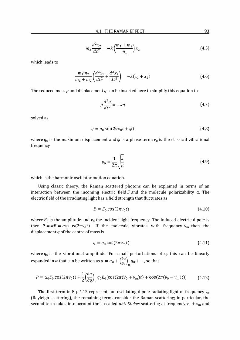
4.1 THE RAMAN EFFECT 93
(4.5)
which leads to
(4.6)
The reduced mass µ and displacement q can be inserted here to simplify this equation to
(4.7)
solved as
(4.8)
where is the maximum displacement and is a phase term; is the classical vibrational frequency
(4.9)
which is the harmonic oscillator motion equation.
Using classic theory, the Raman scattered photons can be explained in terms of an interaction between the incoming electric field and the molecule polarizability α. The electric field of the irradiating light has a field strength that fluctuates as
(4.10)
where is the amplitude and the incident light frequency. The induced electric dipole is then . If the molecule vibrates with frequency then the displacement q of the centre of mass is
(4.11)
where is the vibrational amplitude. For small perturbations of q, this can be linearly expanded in that can be written as , so that
(4.12)
The first term in Eq. 4.12 represents an oscillating dipole radiating light of frequency (Rayleigh scattering), the remaining terms consider the Raman scattering; in particular, the second term takes into account the so-called anti-Stokes scattering at frequency and

4.1 THE RAMAN EFFECT 94
the third the Stokes scattering at . A molecular vibration is not Raman active if the change in polarizability is zero.
The polarizability can be in general described by
(4.13)
where the matrix on the right-side of the equation is called the polarizability tensor. A molecular vibration is Raman active if one of the tensor components is changed during the vibration.
This treatment predicts the Raman scattering frequencies. This procedure involves the application of the classical selection rules for the vibrational frequencies of the molecule of interest, [2] and becomes progressively more difficult as the complexity of the molecule increases. Homonuclear diatomic molecules, for instance, have just one vibrational mode. These molecules have no net electric dipole and the electron density does not change for small perturbations of the relative atomic positions. Therefore, these molecules are not infrared active. Nevertheless, the polarizability is non-zero and can be considered as a combination of the polarizability components parallel ( ) and perpendicular ( ) to the atomic bond. The total mean polarizability is and its anisotropy is . Near the equilibrium position, these quantities are both non-zero for the atoms in a diatomic molecule, which means that the vibrations will be Raman active.
Raman spectroscopy can thus give additional information that infrared spectroscopy can otherwise not provide. These two techniques are complementary and often used together in chemical analysis.
For a complete description of the Raman effect a quantum mechanical model is required. According to quantum theory, a molecular motion can have only certain discrete energy states. A change in state is thus followed by the gain or loss of one or more energy quanta. A quantum energy is defined by , where is Plank’s constant and is the classical frequency of the molecular motion. The interaction of a molecule with electromagnetic radiation can thus be analyzed in terms of an energy-transfer mechanism. For instance, the simplest absorption process involves the gain of a quantum of energy by the molecule, accompanied by the annihilation of a quantum of light. Similarly, spontaneous emission can be described as the creation of one or more photons due to the corresponding loss in molecular energy.
Scattering process involve al least two quanta acting simultaneously in the light-matter system. Simple elastic scattering, also called Rayleigh scattering, occurs when a quantum of electromagnetic energy is created at the same time that an identical one is annihilated. Thus, the molecule is unchanged by the event. In the case of an inelastic process as the Raman effect, two photons are not identical and there is a net change in the state of the molecule. If the created photon is less energetic than the annihilated one, the scattered light is observed at a lower frequency than that of the incident light. This case is referred to as Stokes Raman scattering. On the other and, if the created photon is the most energetic of the two, the Raman
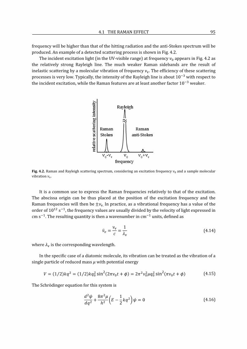
4.1 THE RAMAN EFFECT 95
frequency will be higher than that of the hitting radiation and the anti-Stokes spectrum will be produced. An example of a detected scattering process is shown in Fig. 4.2.
The incident excitation light (in the UV-visible range) at frequency appears in Fig. 4.2 as the relatively strong Rayleigh line. The much weaker Raman sidebands are the result of inelastic scattering by a molecular vibration of frequency . The efficiency of these scattering processes is very low. Typically, the intensity of the Rayleigh line is about with respect to the incident excitation, while the Raman features are at least another factor weaker.
Fig. 4.2. Raman and Rayleigh scattering spectrum, considering an excitation frequency and a sample molecular vibration .
It is a common use to express the Raman frequencies relatively to that of the excitation. The abscissa origin can be thus placed at the position of the excitation frequency and the Raman frequencies will then be In practice, as a vibrational frequency has a value of the order of , the frequency values are usually divided by the velocity of light expressed in
. The resulting quantity is then a wavenumber in units, defined as
(4.14)
where is the corresponding wavelength.
In the specific case of a diatomic molecule, its vibration can be treated as the vibration of a single particle of reduced mass µ with potential energy
(4.15)
The Schrödinger equation for this system is
(4.16)

4.1 THE RAMAN EFFECT 96
Considering the constraint that the wave equation ψ is single-valued, finite and continuous, the solution is
(4.17)
ν being the vibration frequency defined as and . ξ is the quantum number with integer values 0, 1, 2, ... The wave function ψ is
(4.18)
where , and is the Hermite polynomial of the ξth degree. The vibrational frequency is the same as for the classical derivation. The lowest energy state has a value of and the selection rules only allows transitions of
If the incident radiation frequency , the most probable transition is , which is the infrared absorption process (Fig. 4.3 B) The other possibility is the induced emission , schematically shown in Fig. 4.3 C.
If , the incident photon excites an electron to a virtual energy level before going back to to the ground state. This is the case of the Rayleigh scattering - if the exciting energy equals the emitted one - or the Stokes/anti-Stokes diffusion, determined by initial and final energy levels. Phenomena are described in panel D, E and F of Fig. 4.3.
Fig. 4.3. Interaction of a photon with matter: sketch of the possible energy level transitions. Illustration from [2].

4.1 THE RAMAN EFFECT 97
At a given temperature, the energy levels allocation of a molecule follows a Maxwell-Boltzmann distribution. Only the molecules in the excited state will give rise to an anti-Stokes
transition. This is the reason why the Stokes rays are more intense than the anti-Stokes ones. The ratio between the anti-Stokes IAS and the Stokes IS intensities is expressed as
(4.19)
where K is the Boltzmann constant ( ), T is the temperature and is the incident exciting frequency. The samples temperature can be thus calculated by knowing the Stokes and anti-Stokes scattering intensities.
4.1.3 Resonance Raman scattering
The above described Raman effect concerns the so-called conventional or linear Raman effect. This phenomenon can be viewed using a monochromatic UV-visible radiation – in most cases a laser source – that illuminates a sample, and detecting the frequency-shifted Raman scattered light.
The resonance Raman (RR) scattering is a phenomenon that occurs when the excitation light wavelength coincides with – or is close to – the electronic transition wavelength of the molecule or crystal under study. So, rather than exciting the molecule to a virtual energy state, it is excited to a level close to its excited electronic transition. Fig. 4.4 shows the different resonance Raman scattering possibilities.
Since the energy of these transitions differs from one chemical species to the next, in practice this technique was not utilized until the introduction of tuneable lasers in the early 1970s. The advantage of using resonance Raman is a sensible increase in the scattering intensity: when the frequency of the laser beam is tuned to be near an electronic transition (resonance), the vibrational modes associated with that particular transition exhibit a greatly increased Raman signal. This usually overwhelms Raman signals from all of the other transitions.
Fig. 4.4. Sketch of different transition possibilities occurring during the resonance Raman scattering. Illustration from [2].

4.1 THE RAMAN EFFECT 98
Resonance Raman spectroscopy is, for instance, particularly useful for large biomolecules with chromophores, such as haemoglobin: tuning the laser to near the charge-transfer, the iron centre electronic transition results in a spectrum reflecting only the stretching and bending modes associated with the tetrapyrrole-iron group. [3] Consequently, in a molecule with thousands of vibrational modes, RR spectroscopy allows to look at relatively few vibrational modes at a time. This reduces the complexity of the spectrum and permits an easier identification of an unknown protein. Moreover, if a protein has more than one chromophore, different chromophores can be studied individually if their charge transfer bands differ in energy. In addition to identifying compounds, RR spectroscopy can also supply structural identification about chromophores in some cases.
The main advantage of RR spectroscopy over traditional Raman spectroscopy is the large increase in intensity of the peaks in question (by as much as a factor of 106). This allows RR spectra to be generated with sample concentrations as low as 10-8 M. This is in stark contrast to conventional Raman spectra, which usually requires concentrations greater than 0.01 M.
4.1.4 Surface enhanced Raman scattering
Surface enhanced Raman scattering (SERS) was discovered in 1974 by Martin Fleischman and co-workers. [4] They studied pyridine molecules adsorbed on an electrochemically roughened silver substrate and recorded a large Raman signal, justifying it as a matter of the molecule number that were scattering on the surface, without recognizing the major enhancement effect. In 1977, two groups independently noted that the concentration of scattering species could not account for the enhanced signal and each proposed a mechanism for the observed enhancement, which still constitute the underlying principles for the modern theories of the SERS effect. Jeanmaire and Van Duyne [5] proposed an electromagnetic effect, while Albrecht and Creighton [6] proposed a charge-transfer effect.
A flat metallic surface has an electromagnetic resonance called the surface Plasmon,
whose frequency and parallel momentum obey the dispersion relation ,
where and are the metal and ambient dielectric functions. [7] Frequency and parallel momentum must be conserved for a plane wave impinging on the metal surface. This condition can normally not be achieved in air or vacuum; hence a surface Plasmon does not radiate but is confined to the metal surface (its amplitude decaying exponentially with distance away from the surface) eventually dissipating its energy as heat. The plasmon can radiate if the conductive substrate is rough, such as a ruled surface. The Raman intensity scattered by N molecules absorbed on a rough metal surface can be expressed as follows
(4.20)
where is the incident radiation intensity, and are the electromagnetic enhancing factors at the incidence laser frequency and at the Raman scattering frequency
, T is the parameter characterizing the spectrometer transmission efficiency and

4.1 THE RAMAN EFFECT 99
the detector sensitivity; is the scattered angle over which light is collected and is the differential scattering cross section of the molecule vibrational mode .
A rough surface can be modelled as an ensemble of small metallic spheres − with radius − inside a dielectric medium, characterized by the relative permittivity coefficients
and . In the specific case of a metal with independent electrons (Drude’s model), the permittivity is expressed as a function of the plasma electrons frequency . The electromagnetic field of the incident laser beam with frequency induces in the spherical particles a dipole with the same frequency . If , the dipole produces a resonant effect with the sphere and surface modes at and at . The dipole radiated field will induce in the molecule a dipole − vibrating at the Raman frequency − that consequently will generate another dipole in the metal oscillating at the same frequency. These electromagnetic resonances are taken into account in Eq. 4.19 by the terms .
The shape and size of the metal nanoparticles strongly affects the strength of the enhancement because these factors influence the ratio of absorption and scattering events. [8] There is an ideal size for these particles − not just any small particles will have the same impact on the Raman intensity − as well as an ideal surface thickness for each experiment. [9] Particles which are too large allow the excitation of multipoles, which are non-radiative. As only the dipole transition leads to Raman scattering, the higher-order transitions will cause a decrease in the overall efficiency of the enhancement. Particles which are too small, however, lose their electrical conductance and cannot enhance the field. Furthermore, when the particle size approaches a few atoms, the definition of a plasmon does not hold, as there must be a large collection of electrons to oscillate together. [10]
SERS did not achieve improvements in the last ten years and thus did not attract the interest of researchers until Kneipp and co-workers [11,12] and Nie and co-workers [13] simultaneously and independently reported that intense enough SERS emissions could be recorded under favourable circumstances to detect single molecules. In particular, Nie and Emory [13] collected SERS spectra of Rhodamine molecules − commonly used laser dyes − that were incubated with colloidal silver particles and deposited on glass surfaces. The set of measurements proved that the intrinsic enhancement factors in SERS could be as high as
. The need of high-sensitivity molecular- and especially biomolecular-sensing platforms
pushed more and more people to work with surface-enhanced Raman scattering. A recent work published in Nature by Qian et al. [14] in 2008 reports a revolutionary application of near-infrared Raman spectroscopy in medical science: the authors collected SERS spectra at a focal length of 9 mm in a completely noncontact and non-invasive manner on a living mouse. Nanometer-sized golden colloids were conjugated with tumour-specific ligands, coated with PEG and injected in the mouse. Particles accumulated in tumours were detected by SERS even in buried animal tissues.
Two active fields have evolved largely out of SERS: near-field optics [15] and plasmonics [16].

4.2 NEAR-FIELD RAMAN SPECTROSCOPY 100
4.2 Near-field Raman spectroscopy Near-field Raman (or nano-Raman) spectroscopy is the result of the combination between a scanning near-field optical microscope and a Raman spectrometer. It represents one of the few techniques that yields chemical information at nanometre length scales without damaging the sample. Nano-Raman keeps most of the far-field advantages of Raman spectroscopy while sensibly improving resolution and providing simultaneously topographic images to corroborate the optical data.
In 1995 Jahncke and co-workers presented the first Raman images in the near-field. [17] Advances in SNOM imaging in the last years brought consequently great benefits to nano-Raman spectroscopy, resulting in a powerful technique for characterizing material properties, such as localized stress, [18] local chemical and material composition. [19,20]
Nano-Raman can be performed under ambient conditions and no special sample preparation is required. Moreover, the visible light used is not as damaging as more energetic photons or electrons are. Furthermore, the main advantage of nano-Raman resides in the high resolution achievable since SNOM can provide subwavelength optical information an order of magnitude larger than the best conventional optical microscope, i.e., down to . [21,22]
The reason why nano-Raman is not widely used is due to the low signal resulting from the small Raman scattering cross-section added to the SNOM low signal level. However, recent advances have helped to make near-field Raman more accessible: one is certainly SERS, already discussed in the previous section. The other is tip-enhanced Raman spectroscopy (TERS) [23] that allows the acquisition of enhanced Raman signal using a metal coated tip and is thus easily combined to SNOM.
In the next paragraphs we will describe the nano-Raman system designed and developed in our lab. Moreover, preliminary measurements on reference samples will be shown together with a novel application in biology.
4.2.1 Experimental setup
We built a nano-Raman system with the specific aim of mapping the optical and chemical properties of biological samples. A scheme of the experimental setup is shown in Fig. 4.5.
The green-blue 488 nm line of an Argon laser (Koheras, Germany) is selected by a holographic filter (Kaiser optical systems inc, USA) and focused with a 12 cm-focal length-lens on the surface of the specimens under study, mounted on the sample holder of a home-made scanning near-field optical microscope. The scattered light from the sample is collected in the near-field by the small aperture of a gold-coated tapered silica fibre, positioned in close proximity to the surface. A 200X-enhancement camera is mounted on top of the microscope to visualize the specimens to scan and to ensure a correct focus of the laser spot, critical for successful measurements. The collection SNOM has already been described in detail in Chapter 1.
Once collected by the aperture, the scattered light is sent through the optical fibre to a focusing system, with 2 lenses and a notch filter (Kaiser Optical Systems Sarl, France). The coupling light into a spectrometer often demands careful attention: the fibre optic is

4.2 NEAR-FIELD RAMAN SPECTROSCOPY 101
connected on one side of a black cylinder equipped with a rail on which the lenses and the notch filter are fixed, permitting movements only in the horizontal direction. The system special design allows the adjustment of its components’ position by a rotating lateral aperture and ensures a dark environment during measurements. The lenses optimize the focus of the light at the monochromator entrance. The notch filter is a band-stop filter with a narrow stopband centred at 488 nm − the wavelength of the incident beam.
The use of a notch filter is fundamental in Raman spectroscopy since the intensity of the inelastic scattered light, carrying the chemical -specific information about the sample, is very low compared to the intensity of the elastic scattering, occurring with no loss of energy and therefore at the same wavelength of the incident laser. The notch filter stops the 488 nm plasma line before entering the monochromator and consecutively the detector, allowing longer acquisition time and the collection of the Raman peaks. The holographic filter has a bandwidth < 20 nm and the transmission efficiency in the range 350 – 1400 nm is 80%.
Fig. 4.5. Sketch of the nano-Raman experimental setup.
The Raman spectrometer coupled to the SNOM system was bought from Horiba Jobin Yvon, France. It consists of a MicroHR monochromator and a Symphony CCD detecting system. The MicroHR is an automated, compact and versatile Czerny-Turner imaging spectrograph and scanning monochromator, featuring a 140 nm focal length. It is equipped with two gratings – 600 and 1800 grooves/mm – allowing a 0 to 1500 nm scan range and down to 0.2 nm array resolution, i.e., the FWHM wavelength resolution of a spectral line on a focal plane.
The vertical and horizontal slits at the monochromator entrance control both the width and height apertures. The slit width and height directly affects the throughput and wavelength

4.2 NEAR-FIELD RAMAN SPECTROSCOPY 102
resolution of the system, although the former to a higher extent. A height limited slide controls the slit height and has 4 settings: 1 mm, 3 mm, full height (15 mm) and closed. The width can be instead continuously adjusted from 0 to 2 mm with a micrometer slit. For entrance slit widths above 50 µm, the bandpass is defined by the formula:
BP = Linear Dispersion x Exit Slit Width or Image of Entrance Slit Width (whichever is greater).
BP = Linear Dispersion x (pixel Width x 3 pixels) or Entrance Slit Width
(whichever is greater).
The mircoHR specific has been designed to minimize any stray light reaching the focal plane and is free from rediffracted light, i.e., a source of stray light that involves multiple reflections off the optical components themselves and is therefore difficult to mask.
The detecting system is a 1024 x 256 thermoelectric open electrode CCD detector, with an average quantum efficiency of 40% from 200 to 900nm, and a relatively flat response. The thermoelectric cooling system allows a low dark signal operation without the need for liquid nitrogen. The open electrode technology permits an increased response in the UV over standard front illuminated CCDs. The image area is 26.6 mm x 6.7 mm with a pixel size of 26 µm x 26 µm.
Both monochromator and CCD are connected to a PC through a control unit. The user-friendly SynerJY software allows to steer the motorized system, to check the status of each component and to perform measurements.
The Raman spectral acquisition is synchronized with the SNOM scanning using the trigger capabilities of the Symphony controller. A TTL pulse is used to activate the start of each experiment, as well as to initiate the spectral data acquisition of an experiment involving multi-acquisitions. In this way, for each point of the area selected to scan with the SNOM we simultaneously acquire a Raman spectrum. The trigger allows to arbitrary choose the acquisition time for each point of the map: the SNOM scanning system waits until the Raman signal is acquired for the desired time and then passes to the next point.
The result is a correlated data set composed by a topographic and Raman multispectral map: a complete Raman spectrum corresponds for each surface point.
4.2.2 Porous polycrystalline glass-ceramic
Porous glass-ceramic is an inexpensive, easy-to-use material that in combination with metallic monolayers exhibit surface-enhanced Raman scattering properties. Additionally it shows an excellent biocompatibility and can be therefore used as a substrate for biological and chemical analysis.
Pan et al. reported a strong surface-enhanced Raman scattering of Rhodamine 6G dyes adsorbed on silver-coated porous glass-ceramic substrates, [24] demonstrating that they provide a superior support with surface-enhanced Raman signal for both test molecules and silver coating.

4.2 NEAR-FIELD RAMAN SPECTROSCOPY 103
After the development and calibration of the nano-Raman system, due to its SERS properties, we chose the leached porous glass-ceramic sample to perform test measurements.
The porous polycrystaline glass-ceramic was prepared by the controlled glass crystallization (690°C/24h) of CaCO3, TiO2, P2O5 and NaCO3 powders to form the composition 45CaO-25TiO2-3OP2O5-2Na2O (mol%). A postcrystallization heat treatment was performed at 760°C for 48 hours and a final subsequent acid leaching with 0.1 N HCl for 7 days. [25] The original sample was cut in pieces of the size 5 mm x 12 mm and 1-2 mm thick. The surface was polished to create a flat surface. [24]
The CTP − so called due to its main components, i.e., Ca, Ti and P – was provided by our collaborator A. Zavalin from Vanderbilt University, Nashville, USA. Raman micro and nanospectroscopy studies were already performed by Zavalin and co-workers on the same glass ceramic and their work [26] was hence taken as a reference to evaluate our measurements.
The nano-Raman measurements were performed using the experimental setup described in the previous section. The incident 488 nm laser light was focused on an approximate area of 4 mm x 4 mm, and collected by the ~50 nm-aperture of a gold coated silica fibre. The spectrum was acquired for 1000 s with 100 µm slit aperture. Fig. 4.6 shows the recorded Stokes peaks; the abscissa is expressed in Raman shift and counts are in arbitrary units.
The spectrum exhibits the same peaks as the micro- and nano-Raman spectra described in Zavalin’s work [26] and only negligible wavenumber shifts can be observed. However, we report different intensity ratios between the bands. This can be explained by local chemical variations, detected by the nano-Raman system, but not perceived by a micro-Raman spectrometer that illuminates and collects the scattered light from a big area, averaging the eventual variations with the overall signal. This point will be discussed more in detail later.
Fig. 4.6. Nano-Raman spectrum of the CTP ceramic, collected for 1000 seconds with 100 µm slit width. Wavelengths are expressed in Raman shift.

4.2 NEAR-FIELD RAMAN SPECTROSCOPY 104
The Raman shifts are indicated on the spectrum and the characterizing main group assignments are the following: bands at 156 and 648 cm-1 are due to the Ti-O stretching vibration of the TiO2 in anatase form [27]. Peaks at 990, 1019, 1061 and 1106 cm-1 are due to the P-O-P bridging and P-O stretching vibrations in the PO43- network and in the P2O74- groups. [26] It is usually difficult to distinguish the contributions of PO43- and P2O74- bands since there is a strong overlapping of these groups signal, especially of glass ceramics not completely crystallized. [28]
Before using a gold-coated silica fibre, we mounted on the SNOM system an optical fibre that was neither tapered nor metalized. Its aperture thus coincided with the core diameter of the fibre, i.e., ~ 4.7 µm, meaning even 100 times larger than the gold-coated tapered tip used in the subsequent scans. We expected therefore to collect a higher signal with the large aperture.
Fig. 4.7. Nano-Raman spectrum of the CTP ceramic, collected by a single-mode silica fibre (dashed line) and by a tapered gold-coated silica fibre (solid line). Although the acquisition times are the same and the aperture of the gold-coated tapered tip is much smaller than that of the nude fibre, the solid curve exhibit higher intensity, demonstrating that a TERS effect occurs.
Fig. 4.7 shows the nano-Raman spectra of the CPT glass ceramic collected for 1000 seconds by the micron-sized aperture of a silica fibre (dashed line) and by the ~50 nm aperture of a gold-coated tapered fibre (solid line). The latter signal is surprisingly higher although the scattering is collected by a hundred times smaller aperture. This proves that a tip-enhanced Raman scattering (TERS) effect is occurring: taking into account the band around 1060 cm-1, identified for both spectra, the signal collected with the metalized tapered fibre is ~ 11 times higher than the one acquired with the uncoated and untapered fibre. This

4.2 NEAR-FIELD RAMAN SPECTROSCOPY 105
value does not reflect the real enhancement factor – which we hypothesize to be higher – since the two fibres do not have the same aperture size: the uncoated fibre has a wider aperture and thus collects the backscattered light from a bigger area.
The CTP surface, although polished and flattened after cutting, is rough, as shown by the non contact-mode atomic force image displayed in Fig. 4.8: the high-resolution topography (panel A) illustrates the complex structure of a 1 µm2 area of the glass ceramic. The profile 1 is drawn in panel B and shows the height variations. Panel C illustrates the phase contrast image that pictures the changes in the cantilever probe phase angle. This image often provides significantly more contrast than the topographic image and is sensitive to material surface properties, such as stiffness, viscoelasticity, and chemical composition. In our case, the phase contrast image enhances the topographical structure that appears in panel C like a puzzle of different size domains.
Fig. 4.8. A. 1 µm x 1 µm atomic force topography acquired in contact-mode. B. Height profile, corresponding to line 1 in panel A. C. Phase contrast map.
Local intensity variations in the Raman signal can be studied by mapping a similar micron-sized area with the SNOM, while simultaneously acquiring, pixel by pixel, the scattered light.
We selected an area of the CTP: first, we acquired a high-resolution shear-force topography. The same area was later scanned with lower resolution since for each point a 30-seconds-Raman signal had to be recorded. Using the synchronization system described in the experimental section we were able to reconstruct a 10 x 10 pixels nano-Raman map, with a total acquisition time of 3000 s.
The collected data is reported in Fig. 4.9. Panel A shows the first SNOM acquisition, i.e., the 800 x 800 pixels-resolved shear-force topography of a 20 x 20 µm2 area of the glass ceramic. The second scan, performed with lower resolution – a 10 x 10 pixels map represented by the superimposed grid in panel A – resulted in the collection of 100 Raman spectra. In this way, for each specific band we were able to reconstruct the spatial distribution of the Raman intensity. We isolated the gathered signal at 1061 cm-1, where we found the vibrational contribute from the PO43- and P2O74- groups to be the highest. The variation of the vibration intensity is combined with the topography in a 3D map (Fig. 4.9 D), making a direct comparison between the glass ceramic surface structure and the local Raman signal possible.

4.2 NEAR-FIELD RAMAN SPECTROSCOPY 106
The Raman signal at 1061 cm-1 visualized in panel C does not present strong intensity variations: in this area, the vibration of the PO43- and P2O74- groups can be considered constant – within the detection error fluctuations – apart from two spots, where the signal is up to 30% higher than the mean intensity value, and can be attributed to local chemical variation in the CTP composition. Moreover, these differences are not correlated with the topography, as shown in panel D: the two most intense Raman signals are respectively localized on the lowest and highest area of the map.
Furthermore, a conventional microspectrometer, affected by the diffraction limit, would not detect such variations, visible instead to our nano-Raman system.
As already mentioned, the backscattered light was collected for 30 seconds for each pixel. For a more accurate analysis longer integration times are necessary.
Fig. 4.9. A. 20 µm x 20 µm shear-force topography (800 x 800 pixels). B. The superimposed white grid delimitates the area where the Raman signal was extracted from during a second less-resolved scan (10 x 10 pixels map) C. Raman intensity map at 1061 cm-1. D. Combination of the highly-resolved shear-force topography and Raman signal at 1061 cm-1.
The detection of Raman signal variations between nanometre-sized specimens requires a much denser matrix of points, often resulting in extremely long measurements, easier affected by systematic errors and signal fluctuations due to drifts in the SNOM mechanics, tip damaging, ambient condition variations, etc. Surface- or tip-enhanced Raman spectroscopy can overcome this problem, as shown in our measurements.

4.2 NEAR-FIELD RAMAN SPECTROSCOPY 107
4.2.3 Hippocampal neuron cells
The initial goal was to develop a nano-Raman setup to perform nanometre-scale chemical mapping of biological samples.
After the measurements performed on the CTP glass ceramic, we decided that the nano-Raman system was fully operational to pursue our aim and we started working on hippocampal neuron cells. The samples were already described in detail in Chapter 3. In particular, glass-supported neuronal network without fluorophore staining was chosen and studied by near-field Raman spectroscopy.
Fig. 4.10 shows a representative set of measurements, composed by the 40 µm x 40 µm shear-force topography of neuron cell (inset) and Raman spectra collected by the ~50 nm-sized gold-coated fibre aperture positioned on top of the cell body (black spot in the inset, black spectrum), on a neurite (blue spot in the inset, blue spectrum) and outside the cell (red spot in the inset, red spectrum). The scattered light was collected for 1500 s with 500 µm slit aperture. As expected, differences between the Raman spectra taken in different points of the sample are clearly revealed in Fig. 4.11.
The common features found at ~800 cm-1, ~1037 cm-1 and ~2160 cm-1 are partially due to the signal arising from the glass support. This was proved by collecting the Raman scattering from an identical but clean glass coverslip. The glass spectrum is shown in green on top of Fig. 4.10 and was multiplied by a factor 2 to allow a direct comparison with the other spectra. The presence and position of the glass bands are also confirmed by the work of Robinet et al. [29] that reports a Raman spectroscopy study on glass surfaces.
However, considering the high intensity of the peaks around 800 and 1037 cm-1 in the neuron sample spectra, the scattering from the glass substrate can not be considered the only contribution to the resulting bands. The presence of additional peaks from the O-P-O stretching mode and from the C-C skeletal stretching mode, give rise to the intense peaks detected.
There are several works in literature [30-32] showing that the silica fibre also contributes to the total spectrum. We verified that this is true when the probe used has a large aperture or when the overall signal is low and no enhancement due to the surface or the tip occurs. In these measurements, as already demonstrated for the CTP in the previous section, a TERS effect occurs and the silica fibre contribution can be neglected. Moreover, even in the case where the optical fibre give rise to an intense background signal, the silica broad bands appear in the 300-600 cm-1 region, which is excluded from the relevant fingerprint range − 600-1800 cm-1 and 2800-3100 cm-1 – of biological matter.
Fig. 4.11 represents a zoom of Fig. 4.10 ranges of interest: panel A spans from 600 to 1800 cm-1 and panel B from 2740 to 3010 cm-1. As already mentioned, the glass peaks are partially masking additional bands arising from the O-P-O stretching mode and from the C-C skeletal stretching mode that provides direct information on the intramolecular order of the phospholipid aliphatic chains.
The cell body spectrum consists of vibrations from the fundamental constituents of cells: the band at 1230 cm-1 corresponds to the vibration contribution of both the Amide III protein group and the thymine and adenine nucleic acids. Peaks between 1330 cm-1 and 1507 cm-1 are

4.2 NEAR-FIELD RAMAN SPECTROSCOPY 108
attributed to the adenine and guanine nucleic acids, and to the C-H group of proteins. [33] Moreover, bands from 1367 cm-1 can be also assigned to the CH group of lipids.
Fig. 4.10. Raman spectra collected on the neuron cell body (black line), on a neurite (blue line), outside the cell (red line) and on a clean glass coverslip (green line). The intensity of the green spectrum was multiplied by a facto 2 to allow comparison. Inset. 40 µm x 40 µm shear-force topography of a neuron cell.
Fig. 4.11. Raman spectra acquired on the cell body (black line), on a neurite (blue line) and outside the cell (red line). A. Zoom on the range 600 to 1800 cm-1, where the main cell components contribution is found. B. Zoom on the range 2740 - 3010 cm-1. Presence of peaks can be attributed to the lipid contribution.

4.2 NEAR-FIELD RAMAN SPECTROSCOPY 109
The absence of peaks, in the above mentioned range, for the neurite- and outside-spectrum proves that we are able to discriminate between the signal collected on the cell body and the one from the neighbouring structures. In fact, in the neurite spectra, the peak at 1373 cm-1 can be assigned to the C-H group of lipids, which are the main components of membranes. [34,35]
Fig. 4.11 B shows the Raman spectral features of the cell body, the neurite and the specimens outside in the range 2740-3010 cm-1, corresponding to the C-H symmetric and antisymmetric stretching region. As for pure phospholipids, the Raman spectra of nerve fibres in the C-H region are characterized by three unresolved bands at 2850, 2885, and 2940 cm-1, as reported by Pezolet et al. [36] The first two bands are respectively assigned to the methylene symmetric and antisymmetric C-H stretching modes of the phospholipid acyl chains, [37,38] and can be found in all three spectra. The third band arises mainly from proteins, resulting in part from underlying infrared active methylene antisymmetric stretching modes that become Raman active when the intramolecular chain disorder is increased. [38] Panel B clearly shows that this peak (shifted to 2910 cm-1 in our case) is very intense in the cell body spectrum, thus demonstrating a higher protein density, as expected.
Furthermore, it is not surprising that even outside the neuron cell vibrational bands appears: atomic force microscopy topographical maps, showed in Chapter 3, revealed that beneath the neuron cells a vast neuron network grows. The red spectrum corresponds therefore to the signal arising from all the nerve fibres covering the glass coverslip.
Fig. 4.12. Raman spectra collected on the neuron cell body (black and blue line), on a neurite (red line) and outside the cell (green line). Inset. 40 µm x 40 µm shear-force topography of a neuron cell.

4.2 NEAR-FIELD RAMAN SPECTROSCOPY 110
Fig. 4.12 shows another set of measurements. This time the Raman spectra were taken on two spots on the cell body (black and blue line), on the axon (red line) and outside the cell (green line).
Compared to the spectra of Fig. 4.10, the curves in the image above show an overall higher signal. In particular, the peak at 1035 cm-1 is very intense: this could be explained by a stronger glass contribution, probably due to higher tip-enhancement or to a small broadening of the aperture – unavoidable after many hours of measurements.
Apart from the similar features found in the previous set of measurements, pictured in Fig. 4.10, all four spectra present a broad peak at 1445 cm-1 which is assigned to the CH2 deformation mode of lipids.
On the other hand, only the cell body (blue and black curves) presents bands at 970-990 cm-1, assigned to the C-C stretching mode in proteins, and in the range 1655-1680 cm-1 corresponding to the Amide I mode of proteins, [39] proving once again the high sensitivity and chemical resolution of the nano-Raman system.
Four other set of measurements were performed on the same sample, giving similar results. However, in order to confirm the data presented here, a good statistics is needed, implying the study of many more neuron cells and different samples, with longer acquisition time. Nevertheless, our experiments show the great potential of nano-Raman, proven to be a powerful technique for studying cellular biochemistry with high optical resolution.
4.2.4 Ongoing and future work
One of the main challenges faced biology and medicine is the ability to detect and identify a large number of molecules at low concentrations and in short time.
Nano-Raman is a very sensitive technique; it does not require any labelling, and it simultaneously provides detailed chemical and spatial information with a resolution below the diffraction limit. As a noninvasive technique, nano-Raman can characterize the chemistry at specific sites on biological samples with a spatial resolution down to a few 10 nm.
Actually we are still optimizing the experimental setup in order to improve the signal to noise ratio and reduce the acquisition time – still too long to perform highly resolved Raman maps on the entire area instead of few selected points. Moreover, we plan to conclude the study on neuron cells, partially presented in the previous section, and continue the work on peptide-embedded membranes, as discussed in Chapter 2: nano-Raman is the perfect tool to chemically discriminate the amino acids/peptides from the surrounding phospholipids.
The combination of a scanning near-field optical microscope with a Raman spectrometer results in a powerful imaging/chemical analysis instrumentation. Initially the purview of physicist, the nano-Raman is now seen as a valuable tool even for pharmaceutical companies, cell and molecular biologist seeking to link structure with drug or metabolic interactions; chemist working with films, monolayers and multiphase systems, designers of new materials, all of whom need to coordinate chemical information with phase distribution, electrical, mechanical or magnetic information.
This method might be used in future to follow, for instance, the dynamics on cell surfaces, detecting low penetrants in lipid bilayers, or giving insights into the interaction of bacteria

4.2 NEAR-FIELD RAMAN SPECTROSCOPY 111
with their surrounding, including hosts and antibiotics. [32] Furthermore, the technique has the potentialities to localize specific molecules and measure the distribution of proteins, DNA and RNA in cells.
References
[1] Turell, G., J. Corset. Raman Microscopy, Developments and Applications. New York: John Wiley, 1996.
[2] Barbillat, J., D. Bougeard, G. Buntinx, M. Delhaye, P. Dhamelincourt, F. Fillaux. Spectrmétrie Raman. pp. P2865.1-P2865 of Techniques de l'ingénieur. Analyse et caractérisation. Paris: Techniques de l’Ingénieur, 1995.
[3] http://en.wikipedia.org/wiki/Resonance_Raman_spectroscopy [4] Fleischmann, M., P. J. Hendra and A. J. McQuillan. Chemical Physics Letters 26 (2), 163
(1974). [5] Jeanmaire, D. L., R. P. van Duyne. Journal of Electroanalytical Chemistry 84, 1 (1977). [6] Albrecht, M. G., J. A. Creighton. Journal of the American Chemical Society 99, 5215 (1977). [7] Moskovits, M. Rev. Mod. Phys. 57, 783 (1985). [8] Aroca, R. Surface-enhanced Vibrational Spectroscopy. UK: John Wiley & Sons Lt, 2006. [9] Mahurin, L.-L. B. S. M., C.-D. L. S. Dai. Journal of Raman Spectroscopy 34, 394 (2003).
[10] Moskovits, M. Surface-Enhanced Raman Spectroscopy: a Brief Perspective. pp. 1-18 in: Surface-Enhanced Raman Scattering – Physics and Applications. New York: Springer-Verlag Berlin Heidelberg, 2006.
[11] Kneipp, K., Y. Wang, H. Kneipp, I. Itzkan, R. R. Dasari, M. S. Feld. Phys.Rev. Lett. 76, 2444 (1996).
[12] Kneipp, K., H. Kneipp, R. Manoharan, I. Itzkan, R. R. Dasari, M. S. Feld. J.Raman Spectrosc. 29, 743 (1998).
[13] Nie, S., S. R. Emory. Science 275, 1102 (1997). [14] Qian, X., X.-H. Peng, D. O. Ansari, Q. Yin-Goen, G. Z. Chen, D. M. Shin, L. Yang, A. N. Young,
M. D. Wang, S. Nie. Nature biotechnology 26, 83 (2008). [15] Paesler, M. A., P. J. Moyer. Near-Field Optics: Theory, Instrumentation and Applications
New York: Wiley, 1996. [16] Halas N. J. Plasmonics: Metallic Nanostructures and Their Optical Properties. Bellingham:
SPIE, 2003. [17] Jahncke, C. L., M. A. Paesler, H. D. Hallen. Appl. Phys. Lett. 67, 2483 (1995). [18] Webster, S., D. A. Smith, D. N. Batchelder, S. Karlin. Syntetic Metals 102, 1425 (1999). [19] Gucciardi, P. G., S. Trusso, C. Vassi, S. Patane, M. Allegrini. Phys. Chem. Chem. Phys. 4, 2747
(2002). [20] Goetz, M., D. Drews, D. R. T. Zahn, R. Wannemacher. J. Lumin. 76-77, 306 (1998). [21] Pohl, D. W., W. Denk, M. Lanz. Appl. Phys. Lett. 44, 651 (1987). [22] Betzig, E., et al. Science 251, 1468 (1991). [23] Rasmussen, A., V. Deckert. J. Raman Spectrosc. 37, 311 (2006). [24] Pan Z., A. Zavalin, A. Ueda, M. Guo, M. Groza, A. Burger, R. Mu, S. H. Morgan. Appl.
Spectrosc. 59, 782 (2005). [25] Hosono, H., Z. Zhang, Y. Abe. J. Am. Ceramic Soc. 72, 1587 (1989). [26] Zavalin, A., A. Cricenti, R. Generosi, M. Luce, S. Morgan, D. Piston. J. Microsc. 229, 402
(2008).

REFERENCES 112
[27] de Fátima Gimenez, I., I. O. Mazali, O. L. Alves. J. Phys. Chem. Solids 62, 1251 (2001). [28] Dias, A. G., J. M. S. Skakle, I. R. Gibson, M. A. Lopes, J. D. Santos. J. Non-crystalline Solids
351, 810 (2005). [29] Robinet, L., K. Eremin,B. Cobo del Arco, L. T. Gibson. J. Raman Spectrosc. 35, 662 (2004). [30] Takahashi, S., M. Futamata, I. Kojima. J. Microsc. 194, 519 (1999). [31] Jahncke, C. L., H. D. Hallen. 9th annual meeting of IEEE Lasers and Electro-Optics Society
(LEOS) conference proceedings 1, 176 (1996). [32] Neugebauer, U., P. Rösch, M. Schmitt, J. Popp, C. Julien, A. Rasmussen, C. Budich, V.
Deckert. Chem. Phys. Chem. 7, 1428 (2006). [33] Notingher, I. Sensors 7, 1343 (2007). [34] Braun, C. S., G. S. Jas, S. Choosakoonkriang, G. S. Koe, J. G. Smith, C. R. Middaugh. Biophys. J.
84, 1114 (2003). [35] De Gelder, J., K. De Gussem, P. Vandenabeele, L. Moens. J. Raman Spectrosc. 38, 1133
(2007). [36] Pezolet, M., D. Georgescauld. Biophys. J. 47, 367 (1985). [37] Gaber, B. P., W. L. Peticolas. Biochim. Biophys. Acta. 465, 260 (1977). [38] Bunow, M. R., I. W. Levin. Biochim. Biophys. Acta. 487, 388 (1977). [39] Ajito, K., C. Han, K. Torimitsu. Microsc. Microanal. 9, 1062 (2003).

CONCLUSIONS
According to the radiation wavelength and to the material nature, light interacts differently with matter and it is therefore used as a tool to investigate samples chemical and physical properties.
X-rays are used as a probe to study the atomic structure of matter since their wavelength is comparable with the interatomic distances. Infrared light excites molecular vibrations and is employed to investigate the chemical composition of a material. Visible light is used to study the optical properties of a sample, such as the absorbance of light and the fluorescence.
These light sources were used in this thesis work to investigate the order and clustering of lipid bilayers, the structure of model membranes embedded with peptides, the optical properties of neuron cells and the trafficking mechanism of neuron receptors. Moreover, we showed examples of localization of chemical species and molecule clusters, and detection of local chemical variations. Only the combination of methods with different probe-sample interactions allowed us to obtain a consistent and complete characterization of the biological specimens.
We presented X-ray and diffuse scattering measurements on lipid multibilayers, demonstrating that the solid-supported model membranes are well organized along the z axis although not homogeneously distributed on the x-y plane, consisting in ordered islands separated by amorphous regions. The same system was investigated by IR-SNOM using the light of a free electron laser to map the chemical distribution of the lipids, confirming the formation of lamellar-structured bilayers. Moreover, we proved that IR-SNOM not only localizes chemical bonds but also provides real optical signal, giving information about the chemical contents relative concentrations.
The periodicity of highly ordered lipid bilayers allowed to study the solid-supported membranes with energy dispersive X-ray diffraction: the critical role of water molecules in the membrane ordering and assembling process was proved by comparing the diffraction spectra of the same sample before and after full hydration. Furthermore, membrane-peptide interaction was investigated by adding different amounts of the antimicrobial peptide alamethicin to the lipid complex, detecting strong structural changes in the bilayer conformation.
We experimentally studied the distribution of α-amino-3-hydroxy-5-methyl-4-isoxazolepropionic acid receptors (AMPAR) on the surface of new-born rat hippocampal neuron membranes using fluorescence scanning near-field optical microscopy. The transmission micrographs gave information about the optical properties of the internal cell constituents: the most absorbing region, i.e., the densest part of the cell body, was identified as the nucleus. Moreover, the AMPA surface receptors were stained with a fluorophore and detected. The fluorescence patterns in the SNOM images allowed us to study the diffusion of the receptors: from several set of measurements, we observed that the concentration was higher around the densest part of the cell body – the nucleus − and decreased going from this area to the cell borders. From these experiments we hypothesized that after production in the

CONCLUSIONS 114
nucleus the receptors are exchanged through the membrane and diffused along the membrane to reach the synapses. Neuron cells were also studied with infrared nanospectroscopy that allowed the detection of AMPAR clusters at high spatial resolution without any photobleaching problem.
Moreover, we described a method for enhancing fine topographic structures on high relief samples in SNOM images. The approach is based on a gradient transformation of the topography and on the asynchronous acquisition mode for both shear-force topography and SNOM images.
The resolution determination of near-field setups is complex, both from the theoretical and the experimental point of view. In fact, not all the probe and scanning parameters playing a role in the imaging process are exactly known. Moreover, since we are dealing with a scanning probe technique, these parameters can change from one image point to another and lead to different resolving powers of the system. In this thesis work we calculated the resolution of transmission near-field optical images and chemical maps acquired with IR-SNOM using discrete wavelet decomposition. This method allowed a local and precise resolution analysis, such as λ/26 in the mid-infrared range.
In the last chapter we described the combination of a scanning near-field optical microscope with a Raman spectrometer, resulting in a powerful imaging and chemical analysis instrumentation. We first studied a Ca-Ti-P glass-ceramic and later tested the setup on neuron cells.
The use of a gold coated probe placed in the near-field allowed us to collect tip-enhanced Raman scattering, recording an 11-times higher signal than the one acquired with an uncoated fibre. Moreover, local chemical variations were studied by mapping an area of interest: topography and Raman signal were acquired for each scanning point, proving the potential ability of the nano-Raman system to detect chemical information at nanometre scale.
The exceptional sensitivity of the instrument and the ability to localize chemical groups was proved on unlabelled neuron cells: Raman spectra were acquired on diverse areas of neurons by pointing the probe on top of cell bodies, neurites and outside the cells, revealing clear differences in the vibrational bands.
Near-field microscopy has proven to be a powerful investigation tool especially well suited for biological samples: although we have showed only measurements performed in air and on fixed samples, it can work in almost any environment, including liquids, and is totally non-destructive, allowing in vivo experiments. It can perform nanospectroscopic studies, providing a real optical signal with subwavelength resolution.
However, SNOM is still in its early stage: 25 years has passed since the first experimental demonstration1. The interest in the field and the research growth has not been as great as that of other scanning probe microscopes, such as AFM and STM, until the introduction of shear-force based SNOM systems2.
Moreover, in the last few years a renewed interest in near-field optics has appeared. This has not to be attributed entirely to the development of new instruments but to the broadening of the application fields: not exclusively an interest of theoretical and experimental physicists
1 Pohl, D. W., W. Denk, M. Lanz. Appl. Phys. Lett. 44, 651 (1984). 2 Betzig, E., J. K. Trautman. Science 257, 189 (1992).

CONCLUSIONS 115
anymore, SNOM is today used in many disciplines, especially in biological and medical sciences. The ability of imaging in liquid environments and the possibility of performing highly resolved spectroscopic measurements have convinced biologists to approach this technique, contribute to the progress of the discipline, and give a boost towards new research challenges.


117
ACKNOWLEDGEMENTS
My first acknowledgement goes to my thesis advisor, Giorgio Margaritondo; thank you for the total freedom you gave me during these four years: you welcomed every new idea with enthusiasm and showed me the best way to goal. Thank you for all the time spent in front of your computer correcting (rewriting?) my article drafts. This time-consuming training radically changed my writing skills.
I will never stop thanking Antonio Cricenti for his constant support and help, from the very beginning to the end of my PhD. Thanks for the coffee breaks with apple pie and the great pasta dinners that enlightened the otherwise tiring and never-ending-day-and-night beamtimes at the FEL. This thesis work wouldn’t have been the same without your precious advises and suggestions.
Many other people were involved in my work and I want to thank each of them for their help: Norman Tolk, for giving me the opportunity to work in his lab at the Vanderbilt FEL centre; Agostina Congiu, for keeping a fruitful collaboration even after my diploma work; Marco Luce, for his patient support in all the measurements done at the ISM-CNR. Harald Hirling and the rest of the Cellular Neurobiology Laboratory at EPFL, for providing me the neuron samples and discussing the results. I’m specifically grateful to Michel Kropf who took on the unenviable work of initiating a physicist to the world of neuroscience. Thanks to Celine and Christine, always ready to help with a smile.
My days at EPFL and life experience in Lausanne have been enriched by many extraordinary people. Thank you, Vincent, for being such a great office mate (and DJ): I’m not particularly known for my talkative skills and I wonder if anyone else but you could have stood hours and hours of consecutive silence. Thanks Daniel and David, for your contagious optimism and humour. A big grazie to Claudia, for sharing so much and always being there for me; thank you my friends, Silvia and Joy. Thanks to my fantastic roleplaying mates Ana, Anna, Kasia, Gøran and Pablo that many times made me escape from tuff days. Thank you Tamas for the incredible aura of positivism: people should quote you when saying “life is great”. I want to acknowledge my badminton mates Aurore, John and Markus, for avoiding my physical annihilation during the thesis writing. A special merci to Aurore, my neighbour and friend, for all the affection, love and support you shone on me; I have eaten (enjoyed!) more pancakes in the last two years with you than in my entire life. Gracias Camilo, for changing my view of life; breakfast is and will not be the same without you.
I want to thank my acquired (second) family here in Switzerland: Greta, Laura, Luca, Benedetta and Elisabetta. Your home became my little Italy and your love embraced and protected me.

ACKNOWLEDGEMENTS 118
Thanks to my friends back in Rome that, although the distance, supported me and cheered me up ALL the time. Grazie Chiara e Stefano, Chiara, Cristiano e Nicoló Jr, Daniele e Anna.
Tack så mycket to my family in Sweden: your support and understanding is always tangible, no matter where I am.
It is very hard to express by words all my gratitude to my parents, Maud and Renato. Your presence, wisdom and unconditional love followed me like a shadow in easy days, and supported me like a solid rock during hard times.
A big thank you goes to my sister Amanda, my bibina, for the encouragement, deep understanding and constant presence in my life. Even though living far apart, you are still the only person that understands me speaking with a toothbrush in my mouth. Grazie Fabio, for just being as good as you are, making me always feel at home, and bringing out the child in me, sometimes buried inside too much in deep; a big thanks also to little Valle, the new star in the family, for unconsciously enlightening and warming up my days, and for giving me an excuse to play Lego once again.
Last, but definitely not least, my deepest thank to you, Nicoló, my soulmate and best friend, for holding tight my hand during these years and leading me where I couldn’t see. Although apart, you always succeeded in showing me your trust, support, thoughtfulness and love. And it’s exactly in this frame of acknowledgements that I want to reserve a small space also to thank Skype and Expedia, for existing and working so nicely, making my life much easier.

119
PUBLICATIONS AND PROCEEDINGS
During the PhD:
1. J. Generosi, G. Margaritondo, J. S. Sanghera, I. D. Aggarwal, N. H. Tolk, D. W. Piston, A. Congiu Castellano, A. Cricenti. Spectroscopic Infrared Near-Field Microscopy and X-Ray Reflectivity Studies of Order and Clustering in Lipid Membranes. Appl. Phys. Lett. 89, 233906 (2006).
2. J. Generosi, G. Margaritondo, J. S. Sanghera, I. D. Aggarwal, N. H. Tolk, D. W. Piston, A. Congiu Castellano, A. Cricenti. Order and Clusters in Model Membranes: Detection and Characterization by Infrared Scanning Near-field Microscopy. EPIOPTICS-9, Proceedings of the 39th Solid State Physics International School, Erice, Italy 20 - 26 July 2006.
3. J. Generosi, G. Margaritondo, J. S. Sanghera, I. D. Aggarwal, N. H. Tolk, D. W. Piston, A. Congiu Castellano, A. Cricenti. Infrared scanning near-field microscopy investigates order and clusters in model membranes. J. Microsc. 229, 259 (2008).
4. J. Generosi, G. Margaritondo, M. Kropf, H. Hirling, S. Catsicas, K. Johnsson, N. H. Tolk, D. W. Piston, A. Cricenti. AMPA Receptor Imaging by Infrared Scanning Near-Field Microscopy. Physica Status Solidi C 5 (8), 2641 (2008).
5. J. Generosi, G. Margaritondo, M. Kropf, H. Hirling, S. Catsicas, K. Johnsson, N. H. Tolk, D. W. Piston, A. Cricenti. Photobleaching-free Infrared Near-Field Microscopy localizes Molecules in Neurons. J. Appl. Phys. 104 (10), 106102 (2008).
6. B. Lanz, J. Generosi, G. Margaritondo, M. Kropf, H. Hirling, K. Johnsson and A. Cricenti. Fluorescence scanning near-field optical microscopy mapping of the surface AMPA receptors. EPIOPTICS-10, Proceedings of the 40th Solid State Physics International School, Erice, Italy 20 - 27 June 2008. In press.
7. B. Lanz, J. Generosi, V. Gajdošík, G. Margaritondo, M. Kropf, H. Hirling, A. Cricenti. Discrete wavelet analysis used to determine resolution in near-field optical images. EPIOPTICS-10, Proceedings of the 40th Solid State Physics International School, Erice, Italy 20 - 27 June 2008. In press.
Others:
8. J. Generosi, C. Castellano, R. Felici, G. Fragneto, F. Natali, D. Pozzi, A. Congiu. X-ray and neutron reflectivity study of solid-supported lipid membranes prepared by spin coating. J. Appl. Phys. 96 (11), 6839 (2004).
PUBLICATIONS AND PROCEEDINGS 120
9. G. Pompeo, M. Girasole, A. Cricenti, F.Cattaruzza, A. Flamini, T. Prosperi, J. Generosi, A. Congiu Castellano. AFM characterization of solid-supported lipid multilayers prepared by spin-coating. Biochimica et Biophysica Acta 1712, 29 (2005).
10. G. Pompeo, M. Girasole, A. Cricenti, F.Cattaruzza, A. Flamini, T. Prosperi, J. Generosi, A. Congiu Castellano. Optimization of spin-coating-based technique to realize solid-supported lipid multilayers. Japanese Journal of Applied Physics Part 1-Regular Papers Brief Communications & Review Papers 45 (3B), 2310 (2006).
11. C. Esposito, J. Generosi, G. Mossa, A. Masotti, A. Congiu Castellano. The analysis of serum effects on structure, size and toxicity of DDAB–DOPE and DC-Chol–DOPE lipoplexes contributes to explain their different transfection efficiency. Colloids and Surfaces B: Biointerfaces 53, 187 (2006).
12. C. Castellano, J. Generosi, A. Congiu, and R. Cantelli, Glass transition temperature of water confined in lipid membranes as determined by anelastic spectroscopy. Appl. Phys. Lett. 89, 233905 (2006).
13. C. Castellano, J. Generosi, D. Pozzi, R. Cantelli, Anelastic spectroscopy as a probe of dynamic properties in lipid membranes. Materials Science and Engineering A-Structural Materials Properties Microstructure and Processing 442 (1-2): 375-378 Sp. Iss. SI (2006).
14. J. Generosi, M. Piccinini, A. Marcelli, S. Belardinelli, D. Pozzi and A. Congiu Castellano. Characterization of solid supported lipoplexes by FTIR microspectroscopy. Infrared Physics & Technology 50, 14 (2007).

121
CURRICULUM VITAE
JOHANNA GENEROSI
Date of birth: 28 February, 1979 Nationalities: Italian and Swedish
Address: Chemin de la Cocarde 11 CH-1024 Ecublens
Phone: +41 76 308 49 75 E-mail: [email protected] EDUCATION
EPFL – Swiss Federal Institute of Technology, Lausanne, Switzerland Ph.D. in Physics Areas of Concentration: Biophysics and applied physics: structural and chemical characterization of membranes, neuron cells and chromosomes. Atomic force and scanning near-field optical microscopy, infrared and Raman spectroscopy. Free electron laser. Thesis title: Biological Samples Studied by Optical Nanospectroscopy
2005-2009
University “La Sapienza”, Rome, Italy Undergraduate (Bachelor + Master) studies in Physics Areas of concentration: Biophysics: physico-chemical characterization of solid supported lipid membranes. Energy dispersive X-ray diffraction, X-ray reflectivity and diffuse scattering. Synchrotron radiation. Neutron reflectivity. Infrared spectroscopy and microscopy. Thesis title: Structural study of solid supported cationic lipids
1998-2004
AWARDS
Prize for teaching performance, Basic science faculty, EPFL, Switzerland
2007
Fellowship as research assistant in the Laboratory of Biophysics, department of Physics, University “La Sapienza”, Rome, Italy
2004-2005
RELATED EXPERIENCE
Laboratory of Biophysics, University “La Sapienza”, Rome, Italy X-ray Physics Laboratory, EPFL, Lausanne, Switzerland Research activity
2003-present
In detail: My research activity was mainly focused in the field of biophysics and applied physics in collaboration with physicists, biologists and chemists. I learned in deep and used a broad variety of instruments: an energy dispersive X-ray diffractometer, a Fourier transform infrared spectromicroscope, several kind of scanning probe microscopes: atomic force, magnetic force and divers configurations of scanning near-field optical microscopes. I developed a near-field Raman spectroscope. These instruments were used mainly to analyze issues in biology: the physico-chemical properties of biosensors (model

CURRICULUM VITAE 122
membranes, solid-supported lipid-protein systems), the transfection efficiency of gene therapy vectors (lipid-DNA complexes), the receptor distribution in neuron cells, and the localization of chromosomes fragile sites. The results were supported by several measurements performed in synchrotron radiation, neutron source and free electron laser facilities (ESRF and ILL in Grenoble, Desy in Hamburg, FEL centre in Vanderbilt University, Nashville, Tennessee).
TEACHING EXPERIENCE
EPFL, Lausanne, Switzerland Teaching assistant for 3rd and 4th year master students in Physics Title of courses: Physique - Travaux pratiques 3 and 4 (Physics - Laboratory Work 3 and 4)
2005-2009
EPFL, Lausanne, Switzerland Supervision of an undergraduate student diploma work in Physics
2007
CONFERENCES AND SCHOOLS
X-ray and neutron reflectivity study of solid-supported lipid membranes. Oral presentation - Acta Biophysica Romana, 17-18 June 2004, Rome, Italy.
AFM characterization of lipid-multilayer models prepared by spin-coating. Poster session - INFM Meeting 2004, 8-10 June 2004, Genova, Italy.
X-ray and neutron reflectivity study of solid-supported lipid membranes. Poster session - MMD Meeting 2005, 22-25 June, Genova, Italy.
Anelastic Spectroscopy as a probe of dynamic properties in lipid membranes. Poster session - ICIFMS 2005, 5-9 September, Japan.
Infrared and Optical Scanning Near-Field Microscopy Investigates Clustering in Neurons. Poster session - Annual Meeting of the Swiss Physical Society 2006, 13-14 February, Lausanne, Switzerland.
Chemically Resolved Imaging by Infrared Scanning Near-Field Microscopy. Poster session - BMES 2006, 26 April, Lausanne, Switzerland.
Order and Clusters in Model Membranes: Detection and Characterization by Infrared Scanning Near-field Microscopy. Poster session - EPIOPTICS-9, Erice, Italy 20 - 26 July 2006.
Spectroscopic Infrared Near-Field Microscopy Investigates Order and Clustering in Lipid Membranes. Poster session - NFO-9, 10-15 September 2006, Lausanne, Switzerland.
Detection of fluorophore clusterization by infrared nanospectroscopy. Oral presentation - NFO-9, 10-15 September 2006, Lausanne, Switzerland.
From Synchrotron to Free Electron Laser: Characterization of Model Membranes. Oral presentation - SFR07, 18-20 June 2007, Frascati, Italy.
Nanospectroscopic Scanning Near-field Optical Microscopy Investigates Neuron Cells. Poster session - OSI-7 (Optics of Surfaces & Interfaces 7), 15-21 July 2007, Alta, USA.
Scanning Near-field Microscopy and Spectroscopy in Cell Biology. Oral presentation - EPIOPTICS-10, Erice, Italy 20 - 27 June 2008.
LANGUAGES
Excellent Italian (mother tongue) and English (working language). Fluent Swedish. Basic French.


