1

Biological Neurons and Neural Networks,

Artificial Neurons

2

Materi

1. Organization of the Nervous System and Brain

2. Brains versus Computers: Some Numbers

3. Biological Neurons and Neural Networks

4. The McCulloch-Pitts Neuron

5. Some Useful Notation: Vectors, Matrices, Functions

6. The McCulloch-Pitts Neuron Equation

3

The Nervous System

The receptors collect information from the environment – e.g. photons on the retina.

The effectors generate interactions with the environment – e.g. activate muscles.

The flow of information/activation is represented by arrows – feedforward and feedback.

Naturally, in this module we will be primarily concerned with the neural network in the middle.

The human nervous system can be broken down into three stages that may be represented in block diagram form as:

4

Levels of Brain Organization

There is a hierarchy of interwoven levels of organization:

1. Molecules and Ions

2. Synapses

3. Neuronal microcircuits

4. Dendritic trees

5. Neurons

6. Local circuits

7. Inter-regional circuits

8. Central nervous system

The ANNs we study in this module are crude approximations to levels 5 and 6.

The brain contains both large scale and small scale anatomical

structures and different functions take place at higher and lower levels.

5

Brains versus Computers : Some numbers

1. Approximately 10 billion neurons in the human cortex, compared with of thousands of processors in the most powerful parallel computers.

2. Each biological neuron is connected to several thousands of other neurons, similar to the connectivity in powerful parallel computers.

3. Lack of processing units can be compensated by speed. The typical operating speeds of biological neurons is measured in milliseconds (10-3 s), while a silicon chip can operate in nanoseconds (10-9 s).

4. The human brain is extremely energy efficient, using approximately 10-16 joules per operation per second, whereas the best computers today use around 10-6 joules per operation per second.

5. Brains have been evolving for tens of millions of years, computers have been evolving for tens of decades.

6

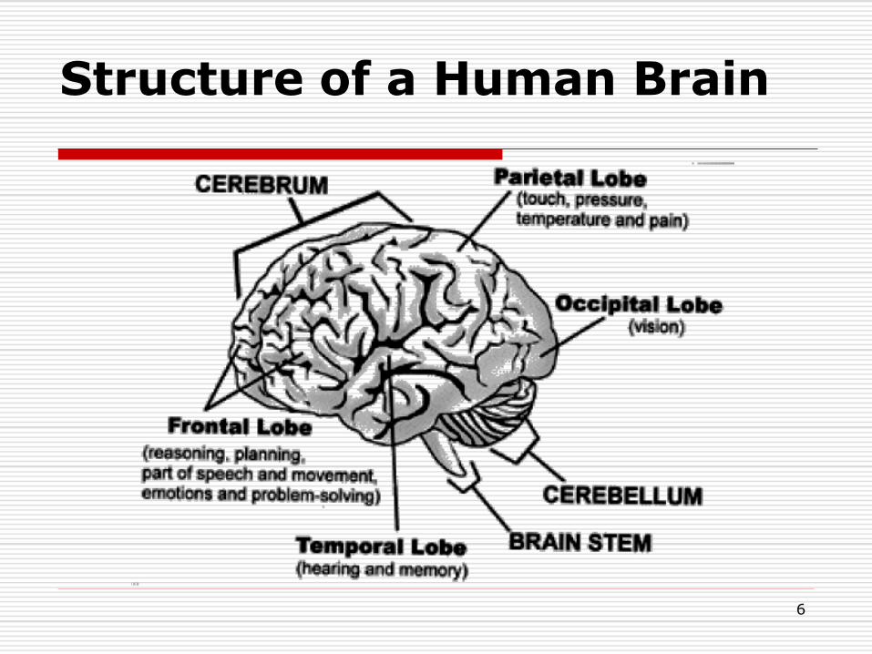
Structure of a Human Brain

7

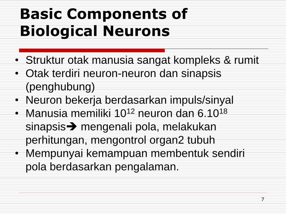
Basic Components of Biological Neurons

• Struktur otak manusia sangat kompleks & rumit

• Otak terdiri neuron-neuron dan sinapsis

(penghubung)

• Neuron bekerja berdasarkan impuls/sinyal

• Manusia memiliki 1012 neuron dan 6.1018

sinapsis mengenali pola, melakukan

perhitungan, mengontrol organ2 tubuh

• Mempunyai kemampuan membentuk sendiri

pola berdasarkan pengalaman.

8

Basic Components of Biological Neurons

1. The majority of neurons encode their activations or outputs as a

series of brief electrical pulses (i.e. spikes or action potentials).

2. The neuron’s cell body (soma) processes the incoming

activations and converts them into output activations.

3. The neuron’s nucleus contains the genetic material in the form of

DNA. This exists in most types of cells, not just neurons.

4. Dendrites are fibres which emanate from the cell body and

provide the receptive zones that receive activation from other

neurons.

5. Axons are fibres acting as transmission lines that send activation

to other neurons.

6. The junctions that allow signal transmission between the axons

and dendrites are called synapses. The process of transmission is

by diffusion of chemicals called neurotransmitters across the

synaptic cleft.

9

Schematic Diagram of a Biological Neuron

10

What are Neural Networks ?

1. Neural Networks (NNs) are networks of neurons, for example, as found in real (i.e. biological) brains.

2. Artificial Neurons are crude approximations of the neurons found in brains. They may be physical devices, or purely mathematical constructs.

3. Artificial Neural Networks (ANNs) are networks of Artificial Neurons, and hence constitute crude approximations to parts of real brains. They may be physical devices, or simulated on conventional computers.

11

What are Neural Networks ?

4. From a practical point of view, an ANN is just a

parallel computational system consisting of

many simple processing elements connected

together in a specific way in order to perform a

particular task.

5. One should never lose sight of how crude the

approximations are, and how over-simplified

our ANNs are compared to real brains.

12

Why are Artificial Neural Networks worth studying?

1. They are extremely powerful computational devices (Turing equivalent, universal computers).

2. Massive parallelism makes them very efficient.

3. They can learn and generalize from training data – so there is no need for enormous feats of programming.

4. They are particularly fault tolerant – this is equivalent to the “graceful degradation” found in biological systems.

5. They are very noise tolerant – so they can cope with situations where normal symbolic systems would have difficulty.

6. In principle, they can do anything a symbolic/logic system can do, and more. (In practice, getting them to do it can be rather difficult…)

13

What are Artificial Neural Networks used for?

Brain modelling : The scientific goal of building models of how real brains work. This can potentially help us understand the nature of human intelligence, formulate better teaching strategies, or better remedial actions for brain damaged patients.

Artificial System Building : The engineering goal of building efficient systems for real world applications. This may make machines more powerful, relieve humans of tedious tasks, and may even improve upon human performance.

As with the field of AI in general, there are two basic goals for neural network research:

14

What are Artificial Neural Networks used for?

These should not be thought of as competing goals.

We often use exactly the same networks and

techniques for both. Frequently progress is made

when the two approaches are allowed to feed into

each other. There are fundamental differences

though, e.g. The need for biological plausibility in

brain modelling, and the need for computational

efficiency in artificial system building.

15

Learning in Neural Networks

One of the most powerful features of neural networks is their ability to learn and generalize from a set of training data. They adapt the strengths/weights of the connections between neurons so that the final output activations are correct.

There are three broad types of learning:

1. Supervised Learning (i.e. learning with a teacher)

2. Reinforcement learning (i.e. learning with limited feedback)

3. Unsupervised learning (i.e. learning with no help)

This module will study in some detail the most common learning algorithms for the most common types of neural network.

There are many forms of neural networks. Most operate by passing neural ‘activations’ through a network of connected neurons.

16

A Brief History of the Field

1943 McCulloch and Pitts proposed the McCulloch-Pitts neuron model

1949 Hebb published his book The Organization of Behavior, in which the Hebbian learning rule was proposed.

1958 Rosenblatt introduced the simple single layer networks now called Perceptrons.

1969 Minsky and Papert’s book Perceptrons demonstrated the limitation of single layer perceptrons, and almost the whole field went into hibernation.

1982 Hopfield published a series of papers on Hopfield networks.

1982 Kohonen developed the Self-Organising Maps that now bear his name.

1986 The Back-Propagation learning algorithm for Multi-Layer Perceptrons was rediscovered and the whole field took off again.

1990s The sub-field of Radial Basis Function Networks was developed.

2000s The power of Ensembles of Neural Networks and Support Vector Machines becomes apparent.

17

ANNs compared with Classical Symbolic AI

The distinctions can put under three headings:

1. Level of Explanation

2. Processing Style

3. Representational Structure

These lead to a traditional set of dichotomies:

1. Sub-symbolic vs. Symbolic

2. Non-modular vs. Modular

3. Distributed representation vs. Localist representation

4. Bottom up vs. Top Down

5. Parallel processing vs. Sequential processing

In practice, the distinctions are becoming increasingly blurred.

18

Some Current Artificial Neural Network Applications

Brain modelling

1. Models of human development – help children with developmental problems

2. Simulations of adult performance – aid our understanding of how the brain works

3. Neuropsychological models – suggest remedial actions for brain damaged patients

19

Some Current Artificial Neural Network Applications

Real world applications 1. Financial modelling – predicting stocks, shares, currency

exchange rates

2. Other time series prediction – climate, weather, airline marketing tactician

3. Computer games – intelligent agents, backgammon, first person shooters

4. Control systems – autonomous adaptable robots, microwave controllers

5. Pattern recognition – speech recognition, hand-writing recognition, sonar signals

6. Data analysis – data compression, data mining, PCA

7. Noise reduction – function approximation, ECG noise reduction

8. Bioinformatics – protein secondary structure, DNA sequencing

Brain vs ANN

20

21

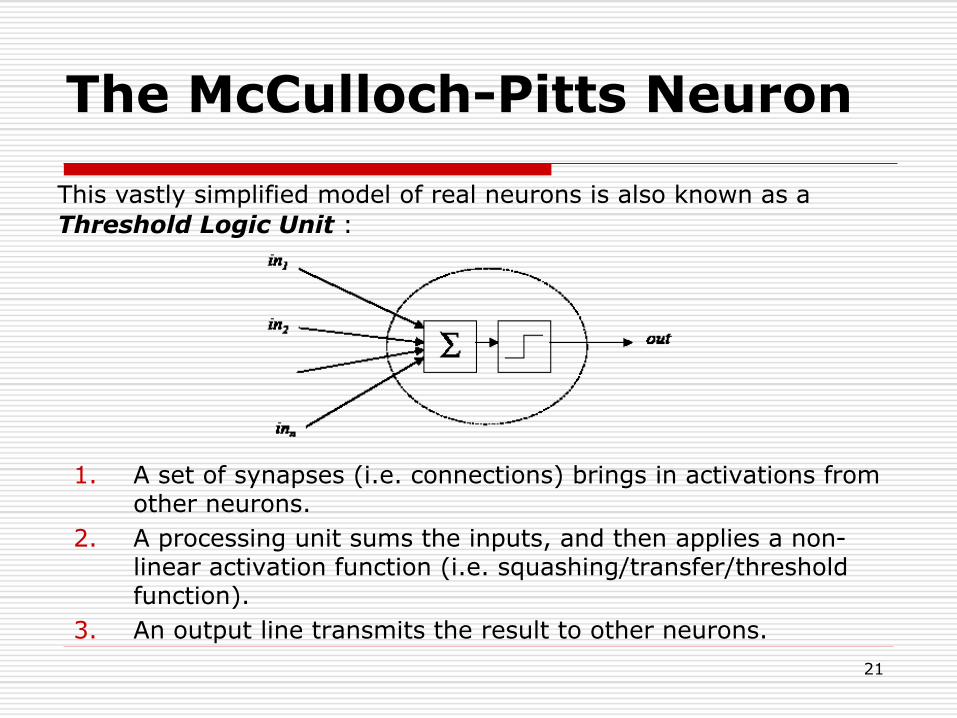
The McCulloch-Pitts Neuron

1. A set of synapses (i.e. connections) brings in activations from other neurons.

2. A processing unit sums the inputs, and then applies a non-linear activation function (i.e. squashing/transfer/threshold function).

3. An output line transmits the result to other neurons.

This vastly simplified model of real neurons is also known as a

Threshold Logic Unit :

22

Some Useful Notation

We often need to talk about ordered sets of related numbers – we call them vectors, e.g.

x = (x1, x2, x3, …, xn) , y = (y1, y2, y3, …, ym)

The components xi can be added up to give a scalar (number), e.g. Two vectors of the same length may be added to give another vector,

e.g.

z = x + y = (x1 + y1, x2 + y2, …, xn + yn)

Two vectors of the same length may be multiplied to give a scalar, e.g.

To any ambiguity/confusion, we will mostly use the component notation (i.e. explicit indices and summation signs) throughout this module.

23

The Power of the Notation : Matrices

We can use the same vector component notation to

represent complex things with many more dimensions/

indices. For two indices we have matrices, e.g. an m x n

matrix

24

The Power of the Notation : Matrices

Matrices of the same size can be added or subtracted component by component. An mxn matrix a can be multiplied with an nxp matrix b to give an mxp matrix c. This becomes straightforward if we write it in terms of components:

An n component vector can be regarded as a 1xn or nx1 matrix

25

Some Useful Functions

A function y = f(x) describes a relationship (input-output mapping) from x to y.

Example 1 The threshold or sign function sgn(x) is defined as

Example 2 The logistic or sigmoid function Sigmoid(x) is defined as

This is a smoothed (differentiable) form of the threshold function.

26

The McCulloch-Pitts Neuron Equation

Using the above notation, we can now write down a simple equation for the output out of a McCulloch-Pitts neuron as a function of its n inputs ini :

where q is the neuron’s activation threshold. We can easily see that:

27

The McCulloch-Pitts Neuron Equation

Note that the McCulloch-Pitts neuron is an extremely

simplified model of real biological neurons. Some of its

missing features include: non-binary inputs and outputs,

non-linear summation, smooth thresholding,

stochasticity, and temporal information processing.

Nevertheless, McCulloch-Pitts neurons are

computationally very powerful. One can show that

assemblies of such neurons are capable of universal

computation.

28

Model Sel Saraf

29

Model Sel Saraf

Sebuah neuron bisa memiliki banyak masukan tetapi hanya memiliki satu keluaran yang bisa menjadi masukan bagi neuron-neuron yang lain.

Pada gambar terlihat serangkaian sinyal masukan x1, x2, …, xp.

Tiap sinyal masukan dikalikan dengan suatu bobot (wk1, wk2, …, wkp) dan kemudian semua masukan yang telah diboboti tadi dijumlahkan untuk mendapatkan output kombinasi linear uk.

30

Model Sel Saraf

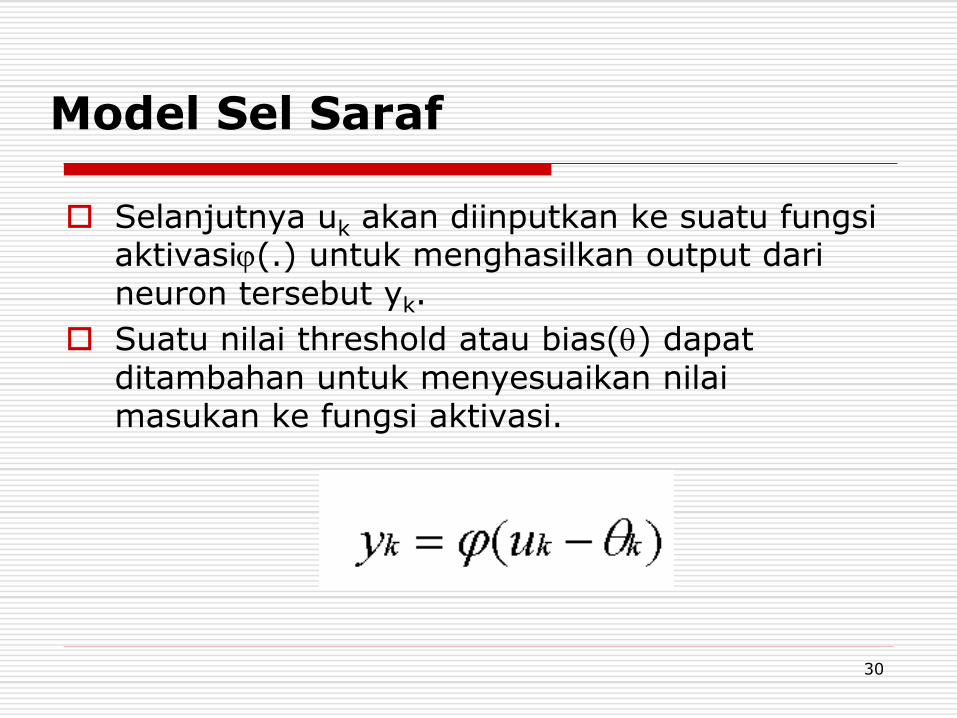
Selanjutnya uk akan diinputkan ke suatu fungsi aktivasi(.) untuk menghasilkan output dari neuron tersebut yk.

Suatu nilai threshold atau bias() dapat ditambahan untuk menyesuaikan nilai masukan ke fungsi aktivasi.

31

Fungsi Aktivasi

Fungsi aktivasi yang dinotasikan dengan (.) mendefinisikan nilai output dari suatu neuron dalam level aktivitas tertentu berdasarkan nilai output pengkombinasi linier ui.

Ada beberapa macam fungsi aktivasi yang biasa digunakan, di antaranya adalah:

Hard Limit

Threshold

Symetric Hard Limit

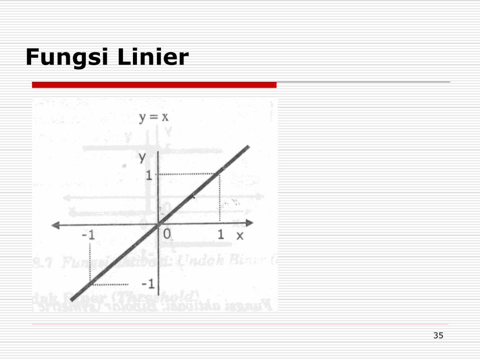
Fungsi linear (identitas)

Fungsi Saturating Linear

Fungsi Sigmoid Biner

Fungsi Sigmoid Bipolar

32

Fungsi Hard Limit (biner)

33

Fungsi Hard Limit (dengan threshold)

34

Fungsi Hard Limit Simetris

35

Fungsi Linier

36

Fungsi Saturating Linear

37

Fungsi Sigmoid Biner

38

Fungsi Sigmoid Bipolar

39

Overview

1. Biological neurons, consisting of a cell body, axons,

dendrites and synapses, are able to process and

transmit neural activation.

2. The McCulloch-Pitts neuron model (Threshold Logic

Unit) is a crude approximation to real neurons that

performs a simple summation and thresholding function

on activation levels.

3. Appropriate mathematical notation facilitates the

specification and programming of artificial neurons and

networks of artificial neurons.