Embed Size (px)
Citation preview

Pallern Recognition Leners 8 (1988) 237-249 Novem ber 1988 North-Holland
Binary contour coding using Bezier approximation
S.N. BISWAS, S.K. PAL and D DUTTA MAJUMDER EIec/ronic and Communica/ion Sciences Unit. Indian S/a/is/ica! Ins/ita/e. Co/cuI/a 700035, India
Received J6January 1988
Revised 28 July 1988
Ahs/raCl: A method for coding of binary image contour using B6zier approximalion is proposed. A set of key pixel (guiding pixels) on the contour is defined which enables the contour to be decomposed into arcs and straight line segments. A set of
cleaning operations has been considered as an intermedIate step before producing the final output.
The quality of faithful reproduetion of the decoded version has been examined through the objective measures of shape com
paclness and the percentage error in area. Finally, the bit requirement and the compression ratios for different input images are compared with the existing ones.
Key words: Contour coding, Bb:ier approximation, Bresenham algorithm.
1. Introduction rithm for approximate coding of binary images based on Bezier approximation technique. A con
Image coding is a technique which represents an tour is first of all decomposed here into a set of arcs image, or the information contained in it with fewer and line segments. For this, a set of key pixels are bits. Its objective is to compress the data for reduc defined on the contour and the vertices of Btzier ing its transmission and storage costs while preserv characteristic triangles corresponding to an arc are ing its information. Various techniques such as spa coded. Regeneration technique involves Bertial domain methods, transform coding, hybrid senham's algorithm [8] in addition to the Bezier coding, interframe coding etc. where both exact (er method. During the regeneration process, key ror-free) and approximate (faithful replica) coding pixels one considered to be the guiding pixels and algorithms for binary and gray tone image have their locations are therefore in no way disturbed. In been formulated are available in [1-8]. Approxi order to preserve them, and to maintain the connecmate coding of gray tone contour for its primitive tivity property some intermediate operations e.g., (lines and arcs of different degree of curvature) deletion and shifting of undesirable pixels generated extraction using fuzzy sets is described by Pal et a!. by Bezier approximation, and insertion of new
[4-5]. pixels are introduced in order to have better faithful
Bezier approximation technique [6,7] which uses reproduction.
J Bernstein polynomials as the blending function Effectiveness of the algorithms is compared with
provides a successful way to approximate an arc two existing algorithms based on contour run
(not having any inflexion point) from a set of length coding (CRLC) [9] and discrete line segment
minimum three control points. The approximation coding (DLSC) (10). The compression ratios of the
scheme is simple and useful for its axis independen proposed methods are found to be significantly im
ce property. It is also found to be computationally proved withoul affecting the quality much when a
efficient. set of images is considered as input. The compact
The present work attempts to formulate an algo- ness and the difference in area between the input
0167-8655/88/$3.50 © 1988, Elsevier Science Publishers B.V. (North-Holland) 237

Volume 8, Number 4 PATTERN RECOGNITION LETTERS November 1988
and output versions keeping the locations of the key pixels the same are also computed to provide a measure of the error.
2. Bezier approximation technique
Bernstein polynomials
The Bernstein polynomial approximation of degree m to an arbitrary function F: [0, IJ ---+ R is defined as
m
Bim[f(t)J = IJU/m) <Pim(t) ;-.:0
where the weighting functions cPi'" are, for fixed t, the discrete binomial probability density functions for a fixed probability,
(m). .<Pim(t)= i "(I-t)"'-', i=O,I, ... ,m (1)
where
111) /111 ( i = (m - i)! i ' .
The remarkable characteristics of the Bernstein polynomials are the extent to which they mimic the principal features of the primitive functionjand the fact that the Bernstein approximation is always at least as smooth as the primitive function j where 'smooth' refers to the numbers of undulations, the total variation etc.
Bezier cUn'es
This class or curves was first proposed by Bezier [6,7]. The parametric form of the curves is
x = PAt), (2a)
Y = P,,(t). (2b)
Let (xo'Y(I), (Xl>YI), ... ,(x""Ym) be (m + I) ordered points in a plane. The Bezier curve associated with the polygon through the above points is the
vector valued Bernstein polynomial and is given by
P,lt) = I. m
¢;m(t) Xi, (3a) r = 0
p!,(t) = L m
<Pim(t) )Ii (3b) i = (I
where <Pim(t) are the binomial probability density
functions of (l). In the vector form, the equations (3) are
P,lt»)pet) - and( Py(t)
so that
P(t) = I m
cPi",(t) Vi (4 ) i = 0
The points Yo, Y1 , ... , \1m are known as the guiding points or the control points.
From equation (4) it is seen that
P(O) = Yo and P(l) = Ym'
Thus the range of t significantly extends from a to I. The derivative of pet) is
ret) = - mel - t)m-l yo
m-l(m)+.I. . {i ti-I(1 - t)m-i '.= 1 I
- (m - i)t i( I - t)m - 1- I} Vi
+ mtm - 1 V . m
Now P'(O) = m(Y I - vo) and P'(I) = m(v", - V _ 1)'m
Thus the Taylor series expansion near zero is
pet) = P(O) + t P'(O) + higher order terms of t ::::: vo(1 - mt) + ...
and an expansion near one is
!pet) = pel) - (1 - t)P'(I) + higher order terms 01'(1 - t)
::::: vm{1 - m(l - t)} + m(1 - t)Y",-I'
It is now clear that as t ---+ 0 the Bezier polynomial lies on the line joining Yo and III and for t ---+ I on the line joining Y". _ I and Y",. This means that these lines are tangents to the curve at Yo and Y",.
238
Volume 8, Number 4 PATTERN RECOGNITION LETTERS November 1988
Also since D'~ 0 ~)i".(l) = I lhe Q~zjel' cUrve lies inside the convex hull of the control point$.
For cubic Bezier curves, m = 3. The control polygon then consists of four control vertices 1'0' Vb 1'2'
V). The Bernstein polynomials for this case are
¢0,3(t)=(l-t))= -t3 +3t l -3t+ 1,
~1.3(l) = Jt(l - 1)2 = 3[3 - 6[2 +3t, cP2,3(t) = Jt 1(1 - I) = - 3t 3 + 3t~,
3cP3.3(t) = t ,
and the corresponding Bezier curve is
P(t) = (1 - t)3 vo + 3t(I - t)21'1
+ 3t2 (1 - t)v2 + t 3 V3 · (S)
Though the cubic Bezier curve is widely used in computer graphics [11] we have used here its quadratic version to make the procedure faster enough.
For the quadratic Bezier curve, m = 2 and the control polygon always consists of three points. The Bernstein polynomials in this case are
cP02(t)=(I-t)2= J -2t+t 2,
cPdt) = 2(1 - t)t = 2t - 2t 2 ,
1>dt) = t 2
Thus
P(t) - [¢",¢",¢,,] [:;]
Vo l = [t
2 t l][c] [ :: J
where the coefficient matrix
J 2 1][c] = - 2 2 a
[ I 0 0
In the polynomial form the Bezier curve is
P(t) = {2(vo + 1'2 - 21'1)
+ 1(2vJ - 21'0) + 1'0' (6)
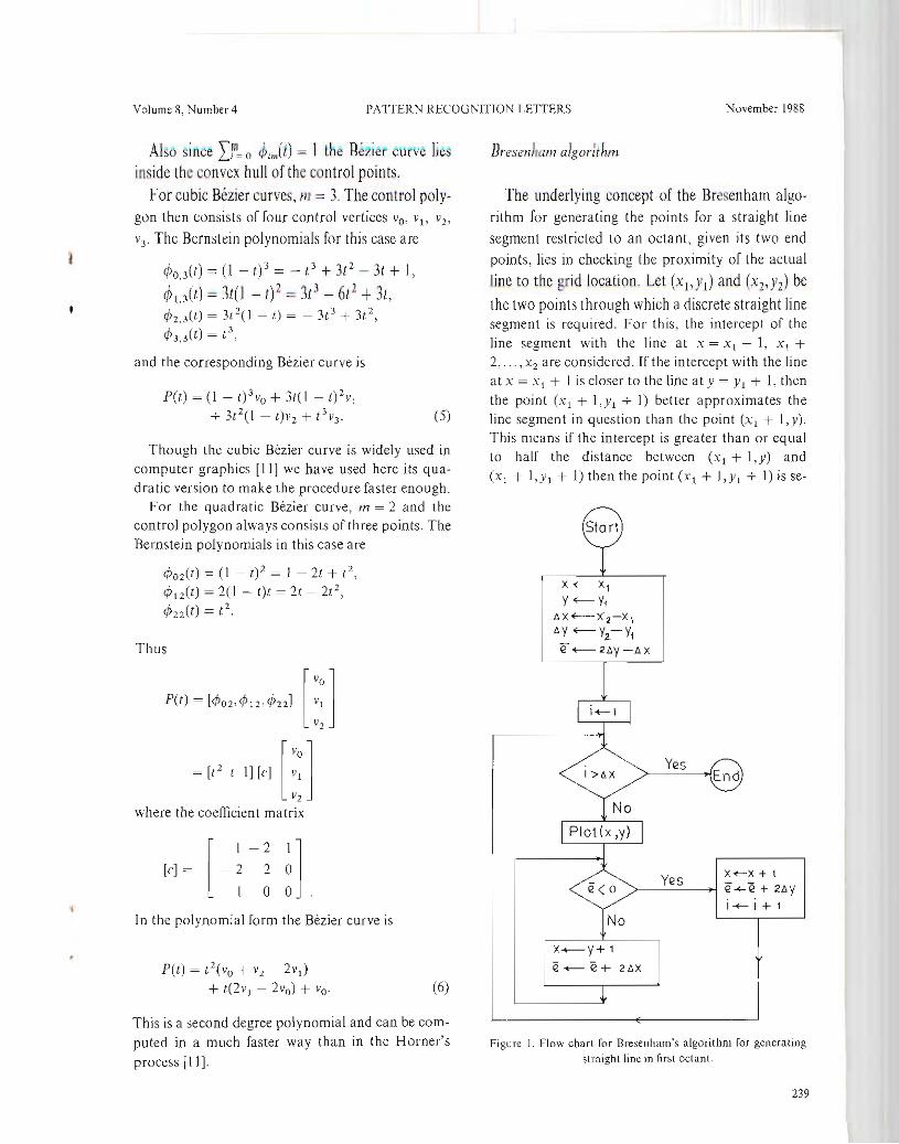
Bresen}rum ulgortthm
The underlying concept of the Bresenham algorithm for generating the points for a straight line
segment restricted to an octant, given its two end points, lies in checking tbe proximity of the actual
line to the grid location. Let (x1,Yl) and (X2,Yz) be the two points through which a discrete straight line segment is required. For this, the intercept of the line segment with the line at x = XI + 1, Xl + 2, ... ,X 2 are considered. If the intercept with the line at X = XI + 1 is closer to the line at Y = Y1 + 1, then the point (x I + 1, Y1 + 1) better approximates the line segment in question than the point (XI + l,y). This means if the intercept is greater than or equal to half the distance between (Xl + 1,y) and
(Xl + I'YI + 1) then the point (Xl + I'YI + 1) is se-
X~Xl
Y~Yj
t>X~-X2-Xj
t>Y <i-- Y2.- Yj
Q +--'2AY-AX
YesI>AX >--------..(End
Yes x~x+ ( ~---~ e+-e + 2AY
1 1 + 1
No
X__ Y+ 1
e+- e+ 2AX
This is a second degree polynomial and can be computed in a much faster way than in the Horner's Figure l. Flow chart for Bresenham's algorithm for genera/ing
slraighlline in first octanl. process [11].
239

Volume 8, Number 4 PATTERN RECOGNITION LETTERS November 1988
lected [or approximation otherwise the point
(Xl + I, y) is selected. Next, the intercept of the line
segment with the line at x = Xl + 2 is considered
and the same logic is applied for the selection of
points.
Now, instead of finding the intercept an error
term, e, is used for the selection purpose. Initially
e = -1 and the initial point (Xl>Yl) is selected. The
slope of the line, /l,yjlh is added to e and the sign
of the current value of e = e + /l,y//I,x is tested. If it
is negative, then the point is selected along the hori
zontal line, i.e. x is incremented by one and y re
mains the same. The error term is then updated by
adding the slope to it. But if the error term is posi
tive (or two), then the point is selected along the
vertical line, i.e. both x and yare incremented by one. The error term is updated by decreasing one
from it.
For integer calcUlation, e is initialized to
e= 2/1,y - /l,x because 2/1,y - /l,x = 2e/l,x = e(say).
The details of the algorithm for the first octant is given in the flow-chart as shown in Figure J.
3. Key pixels and contour approximation
A. Key pixels
In the analytic plane the contour of an object exhibits sharp maxima and minima and these points can be detected almost accurately without much difficulty. However when the contour is digitized in a two-dimensional array space of M x N points or pels or pixels, the sharpness in the curvature of the contour is destroyed due to the information loss inherent in the process of digitization. The error is known as the digitization error. Consequently it becomes rather difficult and complicated to estimate the points of maxima and minima. An approximate solution to this problem is to define a set of pixels, we call key pixels which are close to the points of maxima and minima.
For example, consider a functionf(x) in the discrete plane. When f(x) is constant in an interval [k 1,k2 ], the corresponding analytic function f,(x) may exhibit local maxima and minima (or global maximum or minimum) anywhere within the interval as shown in the Figures 2(a) and 2(b).
y a
: ~l ~ I I I I I I I I
I I I I I ~
I , •
I I : I I
I: I I : I I I I I I I I I I I I I I I
I I I, Ki b\ K 1 l(l. K 2'1"'2,z.. ~\-~I w.,0 'c X
y b
W~ I 1 .! I I I I 1 I I I ~ 1 I I I I I \ I I I I I II I I I I I! I I I III I I I I 1 I! I I 1I I I I I I I ~
0 K;b,K, K1. X
Figure 2. Possible behaviour of/;(x) when j(x) is constant. (a)
Considering local maxima/minima or/,(x). (b) Considering global maximum/mll1imum of f,,(x) . • denotes the position of the
key pixel.
If we get a pixel either direct-connected or outward corner-connected to the end pixels of the interval [k l ,k2 ] such that both the values of/(x) at these pixels are either greater or smaller than its value in the interval, then we assume a point of maximum or minimum to exist at the mid-point of the interval, i.e. at x = (k 1 + k 2 )/2 if (k l + k 2 ) is even
and at x = (k, + k 2 + 1)/2 if (k 1 + k 2 ) is odd. Let us consider this point or pixel in the discrete plane to be a key pixel. Another example for the existence of a key pixel shown by • is depicted in Figure 3 for whichf(x) is not constant over an interval.
B. Definition
A function /(x), constant in [k l ,k2J, in the discrete plane is said to have a key pixel P at x = c
(where c = (k 1 + k2)/2 or (k l + k2 + l)/2 corresponding to even and odd values of (k. + k 2 ))
provided there exist J 1, J 2 E {O, I} such that in both
240

Volume R, Number 4 PATTERN R: OGNITION LETTERS November 1988
the intervals [(k l - bJ ),kl] and [k2,(k2 62)]
either f(c) > f(x) or j(e) <j(x).
When k) = k2 = c, the definition is applicable for
Figure 3 where tJ 1 = tJ 2 = 1. It is to be noted here that the above definition
corresponds to thc Figures 2and 3where key pixels lie on a horizontal sequence of pixels for the interval [k t ,k2] of x. Similarly, key pixels can also be defined
for a vertical sequence of pixels for the interval [k t ,k2] of y.
C. Contour approximation
Let k I ,kz, ... , k p be p key pixels on a contour. The segment (the Geometrical Entity, GE) between two
key pixels can then be classified as either an arc or a straight line. If the distance of each pixel from the line joining the two key pixels is less than a prespecified value, c5, say, then the segment is consid
ered to be a straight line (Figure 4(c»; otherwise it is an arc. The arc may again be of two types, with all the pixels either lying on both sides (Figure 4(a» or lying on the same side (Figure 4(b» of the line joining the key pixels. Let us denote the G E in Figure 4(c) by L (line) and that in Figure 4(b) by ee (curve). It is therefore seen that the GE in Figure 4(a) is nothing but a combination of two eC's meeting at a point Q (point of inflexion).
Therefore, the key pixels on the contour of a twotone picture can be used to decompose the contour into two types of GE's, namely arc and line.
Let us now consider Figure 5 where the curve ee in Figure 4(b) is first of all enclosed within a right
y
o x
Kj
(0) (b)
Figure 4. Types or GE. (a) Arc with inflexion point. (b) Arc. (c)
Slraight 11l1e.
triangle ABC where AC (the line joining k j and k j + 1) is the hypotenuse and A Band BC are the horizontal and vertical lines respectively. It is proved in Appendix A that the arc ee will always be confined within a right triangle ABC. A line DF is then drawn which is parallel to the hypotenuse
AC and passes through the pixel E of maxim um displacement with respect to AC. Thus, the subtriangles ADE and CFE, so constructed, may be taken as the characteristic triangles to approximate the curve ee by quadratic Bhier approximation technIque.
The preservation of the information of Bezier characteristic triangles with the help of key pixels forms the basis of the underlying concept of the proposed coding schemes.
4. Coding schemes
In the proposed method, two points (namely, E and C) are only stored to preserve the characteristic triangles corresponding to an arc when its starting
o A ~ - - .,- - - - - --1 8
" ....... " I '\ ...........'~ I
\, .... E ! " \ 1
" \'\ I \ ' '\ I
" \ ~ F , \ \ I
'\\~! '~~ c
Figure 3. Position or the key pIXel wilen k I ~ k 2 = C. Figure 5. Bezler characteristic lriangles for the arc AEC.
241

Volume 8, Number 4 PATTERN RECOGNITION LETTERS November 1988
point A is known bel'orehand. The point D or F need not be stored because they can automatically
be obtained from the aforesaid points. For example,
D is the point of intersection of the horizontal line
through A and the line through E and parallel to
Af. It is to be noted here that the end point of GE is the starting poinl of Its following GE.
Regarding straight lines, it is obvious that, only
one point needs to be stored when the starting point
is known.
The algorithm for key pixel extraction is shown
in Appendix B.
Bit requiremenl
Let there be p different contours in a binary
image of size M x N where M = 2m and N = 2"The contours may be of two types; either closed or
open. If 11k and ni are respectively the number of key
pixels (including the end pixels for open contour)
and points of inflexion on a contour, then the
number of arcs and straight lines (segments) is (n k + n, - I). Of them, let 11, be the number of straight line segments. For closed contours the initial key pixel is the same as the final key pixel.
The codeword, s, of a GE is variable in length. s consists of two subwords S1 and 52. SI always represents identity (arc or line) of the GE while S2 denotes its description. When the GE is an arc, S2
gives the vertices of the characteristic triangle (for example, A, E, C in Figure 5). For a straight line
segment, S2 indicates the end points of the line segment. It is obvious that the current end point is always the starting point of the succeeding GE. The bit pattern representing a contour is therefore as
displayed in Figure 6.
<---- 1", ----+ <-- r2 -------> <---- 1"3 ------->
[Type or <.:on tour) [Number orGEl [St3rli ng point]
<---- 51 ------> <-- 52 ----+ .................. (Identity ofGE] [Description of GEl
<-- Sl ------+ <----- 52 ----+
[Identlty of G E] [Description orGEl
Figure 6 81t patlern.
242
Types of contours (open or closed) can be repre
sented by a single bit.
In the worst case, all the GE's may be straight
line segments and the number of key pixels may be
MN. Thus it needs (m +n) bits to represent the to
tai number of GE's in a contour.
Identity ofGE (arc or line) can be represented by
a single bit.
Given a starting point of the contour, we need
two points for describing an arc and one point for
a straight line. Each point can be represented by
(m +n) bits. Therefore, for describing an open contour con
sisting of ((n" + I1j - 1) - I1s) arcs and ns lines we
Jteed
To = (m + n) + 2(/11 + n)((nk +fli - 1) - nJ + (m + 11)11.,
bits where the first term corresponds to the starting
point. For a dosed contour, the amount of bits re
quired is Tc = To - (m + n) since the last key pixel
(end point) corresponds to the starting point. From Figure 6. it is therefore seen that To (or TJ
gives the bit requirement for 5 2'S only. The total requirement considering the remaining entities of Figure 6, will therefore be
B,olal = 0. + fJ + ( + /5
where
r;t. = req uirement corresponding to (1 = 1, f3= requirement corresponding to (2
= (/71 + 11.), }' = requirement corresponding to 5/S
= (nk + n; - I), 6= To or Te .
5. Decoding
The coded binary string output corresponding to the method is shown in Figure 7. (m + n) indicates the word length for the number of GE's whereas, (m) + (n) denote the co-ordinates of a point.
Decoding of the string of Figure 7 is based on the following notations.
The first bit (l j) indicates the type of contour (i.e.,
II = 0 for open and 1 for closed). The next sequence

Volume 8, Number 4 PATTERN RE
II /2 IJ 14 1~
H (*** . . *) (*** ... *) (*** .. . *) (*)
(m + n) (111) + (11) (m) + (n)
/6 /~ /5 /6
(*** .. . *) (*** . . *) (*) '-y--J
(m) + (n) (m) + (n)
/4 15 16
(*** ... *) (*) '--v--'
(m) + (n)
Figure 7. Coded binary string outpul.
/2 of (m + n) bits represents the number of GE's present in the contour. The first m bits of the sequence 13 denote the value of the ordinate whereas the remaining n bits give the value of the abscissa of the starting point. Similarly, the co-ordinates of the first key pixel is given by the sequence 14 , Bit /s
says whether the GE between the points represented by /3 and 14 is an arc or a straigh t line. /5 = 0 for line and 1 for arc. If there is an are, then the following sequence {6 is considered to indicate the point E (as in Figure 5); otherwise, the sequence {6
will be absent. As soon as an arc or line is reconstructed, the pre
ceding key pixel point becomes the new starting point.
Thc point designated by the following sequence 14 then represents the new key pixel for further re
construction. The procedure for decoding continues until the
number of GE's, as represented by the sequence 12 •
is exhausted. After that, a new contour is started
with the first bit as 11'
6. Regeneralion lechnique
During the decoding procedure, if the GE between two key pixels is found to be a straight line. then it is generated by the Bresenham algorithm as mentioned in Section 2. If the GE is an are, the
Bezier characteristic triangles are first of all constructed in order to generate its quadratic approxi
mated version.
[TlO LETTER November 1988
RecurSive compuwcion aigorilhm
The algorithm for computing the values of 2nd order Bezier approximation curve using a forward
difference scheme is described below. Let
be a polynomial representation of the equation (6)
where the constant parameters a, band c are determined by the vertices of the Bezier characteristic triangle.
Suppose, a number of points (values of y) on the
arc are to be evaluated for equispaced value of the independent variable t.
The usual Newton's method of evaluating the polynomial results in multiplications and does not make use of the previously computed values to compute new values.
Assume that the parameter l ranges from 0 to I. Let the incremental value be q. Then the corresponding y values will be c, aq2 + bq + c, 4aq 2 + 2hq + C, 9aq 2 + 3bq + c, . ... Let us now form the difference table (see Table I). Observe that
and
for allj z O.
This leads to the recurrence formula Y2 = 2Yl
Yo + 2aq 2 that involves just three additions to get the next value from the two preceding values at hand. Thus one does not need to store all the points on the curve.
Table I Difference table for recursive computation of points of Beziel' curve
y 6)' 6 2y
0 aq2 + bq 2aq 2
q aq2 + bl[ + <: 3aq 2 + bq 2aq 2
21/ 4aq 2 + 2bq + c 5aq 2 + bq 2aq 2
3q 9aq 2 + 3bq + c 7aq 2 + bq
4q \6aq 2 + 4bq + c
243

Volume 8, Number 4 PATTERN RECOGNITION LETTERS Novewoer 1988
7. Implementation strategies
After coding a single pixel wid th contour in pu t, the regeneration algorithm as described before is
used to decode and result in its approximated ver
sion (output). During regeneration, the outer contour is only traced u jng Freeman's ~hain code (clockwise sense) assuring the positions of key pixels on it. In other words, key pixels are considered to be the guiding pixels (being important for
preserving the input shape) during reproduction.
It is to be noted that due to the approximation
scheme, sometimes the following undesirable situa
tions may arise:
(I) The regenerated contour may not have single
pixel width. (2) The key pixel may become an interior pixel of
the contour.
To overcome these situations we trace the con
tours from the orde,red regenerated data set, considering the following operations.
A. Deletion of pixels
During the contour tracing if a pixel on the contour finds more than one neighbour in its 8-neighbourhood domain, then the exterior pixel on the contour is kept while deleting the rest (piXels on the interior contour). But if there is a key pixel falling in such neighbourhood, then the key pixel is retained as the contour pixel and the rest are deleted. This enables us to keep the key pixel always on the contour. thus making the approximation of the input better. Figures 8(a) and (b) depict the situations. Considering 'c' to be the current pixel and 'p' the
previous pixel, the contour (clockwise) is 'a' for a situation as shown in Figure 8(a) but if the situation is as in Figure 8(b) the next pixel on the contour is then k (the key pixel).
a a
pcb pcb
e d e k (a) (b)
d d c c k ~ k b b
a a
(a) (b)
flgurt 9. Shirting or pixels: (a) contour before shirting. (b) con~
lOlIl after shifllJ1l:(.
B. Shifting of pixels
Suppose aGE is generated and a key pixel IS
reached. Now during the generation of a following
G E, its first data point may make the preceding key
pixel lie on the interior contour. For example, considerl-'igure 9(a). Here a h k is part of the
which is already generated. Now generating the
next GE: k c d, ... , the first move from k to c
makes the key pixel (k) lie on an interior contour. In such cases, the data point c is shifted as shown
In Flgurc 9(b). T i~ pre. erves connectedness of the pixel c with both the G E's and also ensures single pixel width of the contour.
C. Undesirable loop
Sometimes in the vicinity of key pixels an undesirable loop (contour with a single pixel hole) may appear due to the approximated generation procedure. For example consider Figure 10. Here GE's a k I k 2 k 3 are already generated. The next move from k 3 to b creates an undesirable loop having single pixel hole
To overcome this situation, the pixel b is shifted along with an insertion of a new pixel e (as shown
d d c c e
b ~ b k 1 k 3 k j k 3
a k 2 a k 2
(a) (b)
FIgure ~. DeleliOn of pixels: (a) in absence or key pixel, (b) in Figure 10. Undesirable loop: (a) before cleaning, (b) after clean
presence of key pixel. ing.
244

•• • • •• • • • •• •
• • • •
••• • • • • • •• • • • • • •
• • •
Volume 8, Numbed P/\TTERN RECOGNITION LETTERS November 1988
in Figure IO(b)). Since the shifting of b alone loses 8. Results and discussion the connectivity property between k3 and the subsequent pixels, it necessitates an insertion of a new Figures 11(a), 12(a) and 13 show the digital conpixel whose location is governed by the concept of tours of three different figures, namely, butterfly, minimum connected path. chromosome and numeral-eight, which were eon
1 00 I Q() 00 000 00 00 J
o o 00 00 0 o o 0 0 o 0
3 000 ) 000 o 000 o 0 o 0 o o 3 3 o 0 0
o o 3 o 0 o o 3 3 0 0
o c o o
o o o 00
o 3 3 o c 3 o 0
o 0 o o 0 o 0 c: o 3 o 0 3 t 0
o o 0 o o 0 o o 0 o o c:
o c: G 3 o 00 o 0 3 o 00 3 0 0a
3 ••• ••••• 3 •
• •• • • 3
• • 3 •• • ••• • •
J • • •
3 • • •
•• • 3
••• • . •) 3 ••• J
•J
• • •J
• •• J
• •• J ••• •• J Jb •
00000303 0 0 0 o 9 0 3 o 0 0
o 0 000 o 0 0 o 00 ,0 0 0
3 003 o d 0 o o 00 0 o 0 0 0 o 80 93 1 0 0
o X 9 El 1 88 X 0 o X ] 3 X 0 o 3
o o o
o
o 8 0 09 J 0 1 0 0
o 0 X 3 3 8 0 o 83 X 8 X 0 0 o 0 o x 0 0 Q o ] 00) 1 0 o 8 o 0 0 0 080
o 000 080 o 8 0 ) o 0 0
o 8 8 0 OOJOOO
C DO 3 J 0
figure 11. (a) BUBerRy input. (b) Regenerated version. (e) Regenerated version before cleaning.
245
• • • • •
• • • • • • •
• • • • • • • • • •
• • • • • • • • • • • • •
• • • • • • • • • • • • • •
Volume 8, Number 4 PATTERN RECOGNITION LETTERS November 1988
00 J 00 ••• J ••• 0 00
0 0 o ) 0 0 •• •• •• J I' 0 a 00 a
•I
••j
• •J 0 0 a 0 0 0 a
0 0 0 3
0 0 0 0 • • •1
0 0 0 0 0 0 x 0
• • 1•I
0 0 0 0 I 0 0 0 0 I •0 0 0 0
0 0 0 0 • • • I
I I 0 0 1 I • I •
0 0 0 0
0 0 0 0 0 0 0 0 • • I
• 0 0 0 0 Q o J 00 0 • • J ••
0 0• ,•• ,
0 0 I 0 0 ,
• • 0 0 0 0
•I
0
J
0
• •() 0 )
0 0 J
• 0 0
•0 0 • • 0 0
•0 o ] 0 0 • 1151 ••
0 0 0 0 I• , • •0 0 0 0
0 0 0 0 I I 0 0 0 0 I
0 0 0 0 0 0 0 0 0 J 3 0 J ] I•
0 0 0 0 I I ••, I0 0 0 0
J 0 0 0• I I
0 ] J 0 ] 0 0 0 0 0 a 0 3
• • l •• J• • I •
0 0 0 0 0 0 3 0 0 0 0 0 0 0 0 0
0 0 0 0 • • '.• • 0 0 0 0 • • ,0 0 0 0 b • ••
.' •a 0 0 0 0 I • o 3 0 0 0 ·.) .. • •
00 0 o ) 0 I 3 •
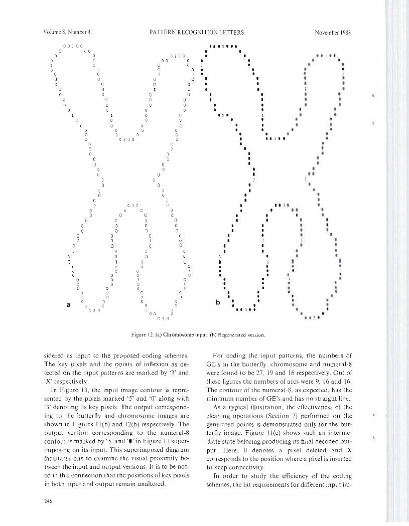
Figure 12. (a) Chromosome input. (b) Regenerated version.
sidered as input to the proposed coding schemes. The key pixels and the points of inflexion as detected on the input patterns are marked by '3' and 'X' respectively.
[n Figure 13, the input image contour is represented by the pixels marked '5' and '0' along with
'3' denoting its key pixels. The output corresponding to the butterfly and chromosome images are shown in Figures II(b) and 12(b) respectively. The output version corresponding to the numeral-8
contour is marked by '5' and '.' in Figure 13 superimposing on its input. This superimposed diagram facilitates one to examine the visual proximity between the input and output versions. It is to be noted in this connection that the positions of key pixels in both input and output remain unaltered.
For coding the input patterns, the numbers of GE's in the butterfly, chromosome and numeral-8 were found to be 27, 19 and 16 respectively. Out of
these figures the num bel'S of arcs were 9, 16 and 16. The contour of the numeral-8, as expected, has the minimum number of GE's and has no straight line.
As a typical illustration, the effectiveness of the cleaning operations (Section 7) performed on the generated points is demonstrated only for the butterfly image. Figure II (c) shows such an intermediate state beforing producing its final decoded out
put. Here, 8 denotes a pixel deleted and X corresponds to the position where a pixel is inserted to keep connectivity.
fn order to study the efficiency of the coding schemes, the bit requirements for different input im
246

Volume 8, Number 4 PATTERN RECOGNITION LETTERS
1 .. ,,\1\\1.1. "SSQOOOO 00001\'.1
I • ~ 0 0 U 0 0 'j 5 •• I , a 0 On':l l) S
• I {) U \ \ , 00 \ \
1 \ 0 \. I 0 OS, • 0 o ,
i I ·.0" o • 5 ••• t 5 j') 5 •• I' o •
10 ••• II 00 () OOOU.II 0(1 • 5 0\ 000 000 \. o • \ o • o •
• 0\ \ 01 o I J 10 \ a I \ ~ 01 \ s ) 5 5 to \ ) )
10 I 0 5 \ ; .0 , 5 ; S o I 01 s S O'
• 0; ,.. • ,0
S S
• 0 5 o I ; 5 .0 lj. 0 0 5 5, lOa O~. a •
• 0 • I 5 0 0 S I a • ; • S )SS, 00' • 0
"ICG e,. I
I 00 O'• t. o •
• 00 (J (II.•••• 0 " ., I •
• • • • 0 • (·0 '; ....
•• 01)
.; "• (I
~J 0 • • 0 0 ',.) 0 •
I 0 J:' 1.1 • o 0 I•• 0 0-:) I) 000 5 ':. • O.
10-0
• •• 5
o I • o S • U SO 0\1 I" ; a I 5
I 0 , ". 01 I I
.0 G 1 a I o • ,• 0
I s O. O'
10• 0 • 0 S o • ,.0
•\
U SJ
.0 ), \ ; o •
5 o • • ') 0 •S • 0 5 O. J 5 n • n I ;
• a ; O. ;
O'• 0 s01 '0 0 • o I 5 S.
lj. 0 00 5 01
, S " .
; tODD 00 • o •I G "'000 00'" O'I ••• ~ 3 ~ S • I o •
10 r • \ o •
5 \ I S
OS \ , 0 I;
SGO 5 5 • 101) ';. ')
•• :.0000 ss I'I'~OOOO OOSSS
• ••• 5 S '-' ] 5 5 ~ ••
Figure 13. Numeral-8 input and its regenerated output together.
ages and their relative compression ratios are compared with those in the CRLC and DLSC methods. It is shown in Table 2 that in the proposed tech Table 2 nique, the bit requirements are significantly less. It Bit requirement
is ohvious that the numeral-8 image consisting of BH requirementfew large arcs only provided higher compression
ratio. The butterfly image on the other hand, has Figure CRLC DLSC Proposed the largest number of GE's and thus provides method lowest compression ratio.
Butlerfly 799 53l 435As the coding schemes are approximate the regenerated image deviates from its original version. Chromosome 1175 603 452
To observe the deviation of regenerated image qual NumeraJ-8 2085 1169 474 ity through an objective measure we have ealculat-
November 1988
c5r~' 9b °rel% (reI. (reI. CRLC) DLSC)
183.67 122.06
259.95 133.40
439.87 246.62
247

Volume 8, Number 4 PATTERN RECOGNITION LETTERS November 1988
Table 3
Error in regeneration
"lgure ;'0 Error in area Compactness
Proposed Ori~inal Generalerl
melhod figure figure
BUlterfiy 8.63 0024635 0.025393 Chromosome 6.8 0.016061 0.016672 Numeral-8 2.92 0.014728 0.Ol4589
cd the error in area and the shape com pactness. For the calculation or the area and the perimeter of the contour we have used the technique proposed by Kulpa [12]. Since the key pixels are always ou the contour and the gcnerateo arcs are between them
and restricted by the respective Bezier characleristic triangles, the maximum error for an arc is the area or its pair of Bezier characteristic triangles. Also, for the above constraint the shape compactness can proviJl: a good measur f the tlistoJ'tion introouced into the decoded images. Table 3 shows hoth the percentage error and the compactness of figures. Tt is thus seen that the decoded image in each case
is a faithful reproduction of its input version. Here too, the butterftyjnumeral-8 contour having the
largest/smallest number of GE's incurred highest/ lowesl %error in their regeneration.
Finally, it is to be mentioned here that since the
regeneration proced ure uses the quadratic Bezier approximation technique, the decoded image display is very fast.
I\cknowledgn cn
The authors would like to thank Mr. J. Gupta
and S. Chakraborty for rendering the secretarial help.
Refe ellces
[I] Proc. JEfF. (1980). Special issue on Computer Graphics, Vol 68.
[2] Ekstrom. M P., Ed. (1984). Dil;ilV/ fmu!!,e Proce.mn!! Tech
/1Jques. Academic Press. New York. [3] Huang, T.S. (1977). Coding of two-lone images. JEEE
Trum. COI1!. 25, 1406-1424.
[4] Pal, S.K., RA King and A.A. Hashim (1983). Image description and primitive exlractJOn USIng fuzzy sets. JEEE
Trans. Sysl. tv!all Cybernel Ll (f), 94-100. ISJ Pal, S.K. and D. Dulla Majumder (1986). Fuzzy Mathemat
ical Approach 10 Partern ReCOiini/lOn. Wiley, New York. 16] Bhier, P.E. (1974). Mathematical and practical possibilities
of UNISURF. In: Barnhill. R.E. and R. F. Riesenletd, Eds.,
COl11pwer Aided Ceomelric Design. Academie Press, New
York. l7jlhrskcy, 9.A. (l9gJ). A Jcs<:riplion anJ evaluation of va
rious 3-D models. In: Kunll, T.L., Ed., Computer Graphics (lheory and app/icalions). Springer, Berlin.
[8] Breselllam, .I.E. (1965). Algonlhm for 0 uteI' control or a digital plotter. fBi'v! S)'S I. em \ 1. 4 (1),25-30.
[9] Morrin, T. H. (1976). Cham link compressIOn of arbitrary
blaek while images. (OI11PUIet' Graph;cs and lmaf?e Procnsillg 5, 172-189.
[10] Chaudhuri, B B. and M.K. Kundu (1984), DIgital line seg
ment coding: A new efficien t contour cod iug scheme It:t; PI'QC 13\ (4), PI E, 143147.
[IIJ Pavlidis, T. (1982). Algoriilllns[or GraphiCS and Image Processing. Springer, Berlin.
[12] Kulpa, Z. (1977). Area and perimeter measurement of blobs
in discrele binarv pictures. COmplller GraphICS and Jmage
J.'rocesSInf? 6, 434-4) I.
Appendix A
Proposition 1. In the discrete plane all the pixels on an arc hetween two key pixels remain always on or inside a right triangle with Ihe line joining lhe key pixels as the hypotenuse. The other two sides of the right triangle are the horizontal and the vertical lines through the key pixels.
Proof. When the key pixel is on the horizontal line at x = c it follows from the definition of key pixel, that
either Fc) >j(x) or fCc) </(x)
in both the intervals [k j - 0t,klJ and [k1,k1 + 62]
wheref(x) is constant in [k l ,k 2J and 6[,62 E{O, I}. Thus
(I) Pixels at k I and k I are ei ther corner connected or direct connected or its combination to the neigh
bouring pixels outside the interval [k1,k1l
(2) When k, = k2 = c, the key pixel will have at least one corner connection to its neighbou ring pixels,
248

Volume 8, Number 4 PATTERN RECOGNITION LETTERS November 1988
c,....-----~'?"""'T-0
1\
Figure A I. An arc with ils associated right triangle.
Similar arguments hold when the key pixel lies on a vertical line.
Let ANB be the arc with A and B being two successive key pixels as shown in Figure A l. Now a pixel on the arc can go outside the line AC or BC
if and only if (1) there exists a sequence of collinear pixels such that its end pixels are either corner connected or direct connected or its combination, or (2) there exists a pixel which has at least one corner connection with its neighbouring pixel.
Both these conditions lead to the existence of another key pixel outside the line A C or Be. This is a contradiction.
Appendix B
A19orithm for extraction ofkey pixels
{P,};'= I are the contour points in the binary
J 2
5 •
6 7 B
Figure B1. Direelional code5 with respeclto •.
image and {(Xi'y;)};'~ 1 are their position co-ordinates. Since, for a closed contour, there is a possibility of missing the first key pixel we need to examine a few more points after the starting point is
reached so as to enable one to get the same back.
P
Step 1. Set i +- I, count +- I. Find the initial direction code between Pi and
j + 1 according to Figure BI. Let it be d j'
Step 2. Increment i +- i + I; if i = n go to Step 7; otherwise find the directional code betwcen Pi and
P, + l' Let it be d2 ·
Step 3. If d l = d2 go to Step 2; otherwise if d , div
2 = 0 and d2 div 2 = 0 or if I d1 - d2 1 = 3 or 5 then
return (Xi, Yi)' Step 4. Increment i +- i + I; if i = n go to Step 7;
otherwise find the direction code between Pi and
Pi + l' Let it be dJ .
Step 5. If dJ = d2 then count +- count + 1 and go to Step 4; otherwise if Id l - d J 1= 0 or I then set count +- I, d j +- dJ and go to Step 2 else do Step 6.
Step 6. If count div 2 = 0 then return (Xi - counl/2,
Yi - counl/2) otherwise return (Xi - counl div 2,Yi - coun' dh 2)'
Step 7. Stop.
249