Embed Size (px)
Citation preview

00I
0 "_ A__0R__0R
TECHNICAL REORBin" REPORTNO. I
I l -* .. ANAW7SI OF 11kCfAOICAL SYSTh(S
Interim Report o T16 June 198110
IDEC i T- 8tI Contract No. DAAK30-78-C-0096
Rajiv Raupalli & EdadJ.Hu
Colgeo EngineeringTh University ofIowa
I University U .qW# Rept. No. 60
.~ .by. RsolR . EBek. Proji.F Englaer, TACoK i
Approved for public release; distribution unlimited.I
U.S. ARMY TANK-AUTOMOTIVE COMMAND
RESEARCH AND DEVELOPMENT CENTERWarren, Michigan 46090 8 12
- -i-l m
I J

DISCLAIMER NOTICE
THIS DOCUMENT IS BEST QUALITYPRACTICABLE. THE COPY FURNISHEDTO DTIC CONTAINED A SIGNIFICANTNUMBER OF PAGES WHICH DO NOTREPRODUCE LEGIBLY.

a' V
NOTICES
The findings in this report are not to be construed as an official Departmentof the Army position,
Mention-of any trade names or manufacturers in this report shall not beA construed as advertising nor as an official endorsement of approval of suchproducts or companles by the U.ot Government.
Destroy this report when it is no longer needed. Do not return it to
originator.
j j J l l ll

UNCLASS IF IEDSECURITY CLASSIICATION OF THIS PAGE ltWon Date ffntoered
REPORT DOCUMENTATION PAGE BEFRE ONsTUTINFR___________________________________ BE FORECOMPL[.ETING FORM
1. REPORT NUMBER 2. GOVT ACCESSION NO. 3. RECIPIENT'S CATALOG NUMBER
12589 VoD -1i'->4. TITLE (and Subtitle) S. TYPE OF REPORT & PERIOD COVERED
Kinematic Analysis of Mechanical Systems Interim to Dec. 79
S. PER!CPR ING ORG. REPORT NUMBER
7. AUTNOR.) 8. CONTRACT OR GRANT NUMBER(&)
Rajiv Rampalli & Edward J. Haug DAAK30-78-C-0096University of IowaRonald R. Beck. TACOM
S. PERPORMING ORGANIZATION NAME AND ADDRESS 10. PROGRAM ELEMENT. PROJECT. TASKAREA & WORK UNIT NUMBERS
The University of IowaCollege of EngineeringIowa City. IA 52242
I1. CONTROLLING OFFICE NAME AND AODRESS 12. REPORT DATE
US Army Tank-Automotive Command R&D Center 16 June 1981Tank-Automotive Concepts Lab, DRSTA-ZSA IS. NUMSEROF PAGESWarren, MI 48090 65
14. MONITORING AGENCY NAME 4 AOORESS(SI diffeon hmn Comtolling Offlc) IS. SECURITY CLASS. (o thle report)
Unclassified
OSI. DEC ASSI FIC ATI ON/ DOWN GRADINGSCM EDULE
IS. DISTRISUTION STATEMENT (of ti. R PW)
Approved for public release; distribution unlimited.
17. DISTRIBUTION STATEMENT (of the a etract entered n Block 20, if different hom R"or)
IS. SUPPLEMENTARY NOTES
IS. KEY WORDS (Continue on ,eoeee Wd It neeoeiar and identify by block nhmber)
Dynamics, Bodies, Response, Control, Interaction, Stability,
Lagrangian Function, Matrices
2& A7WACT' (C~te a mrewae b N n- a Idenit", bbiah monk )
_ ' It is intended in this report to develop a method of kinematicallyanalyzing mechanical systems. A computer code that automatically generatesa set of nonlinear equations describing the system and solves them, is devel-oped. To demonstrate the accuracy and effectiveness of the method to bedeveloped herein, five sample problems have been solved.
While all the sample problems solved are closed-loop mechanical systems,the method described here need not be confined to closed loop mechanical
W Ji7 W3 ENTION OF I NOV 0B It OSmLETE r /
SECUMYP CLASSIFICATION OF THIS PA6E (SS1om Date Enflt~Sl

UNCLASS IFTEDSECURITY CLASSIFICATION OF THIS PAGE(Uhm Doe i gewn
systems or to mechanical systems at all. In fact, the method is applicableto any system whose motion is to be described, provided adequate constraintscan be incorporated into the code by the user. Examples of such systems areelectro-mechanical systems with relays, switches, etc.
Given the topology of a system, the necessary inputs, the method iscapable of computing velocities, positions, accelerations and constraint forceson the system.,/
Briefly, the most notable features of this method are:(i) Complete generality in the derivation of the constraint equations and
computation of the generalized co-ordinates.(ii) Use of sparse matrix subroutines to realize substantial savings in
core when problems of large magnitude are analyzed.(iii) Versatility to incorporate nonstandard constraints into a problem,
if supplied by the user.(iv) Ability to handle constraints, when they are supplied as a set of dis-
crete points, by constructing a third-order spline function through them(v) Ability to perform kineto-static analysis of a mechanical system if
the system is kinematically indeterminate.
.
SECURITY CLASSIFICATION OF THIS PAOR('hn Date Entlorf)

0
Paa.200 >
E- .- 4
W1.4
TABLE OF CONTENTS
Page
LIST OF SYMBOLS ............ ......................... v
LIST OF FIGURES ............ ......................... vi
LIST OF TABLES .......... ......................... .. vii
CHAPTER
I. INTRODUCTION .......... ........................ ....
1.1 Introduction ........ ..................... ... 11.2 Statement of the Problem ...... ............... .11.3 Literature Review ....... ................... . .11.4 Organization of the Report ....... .............. 5
II. AN OVERVIEW OF THE DADS PROGRAM ....... .............. 7
2.1 Lagrange's Equations for Constrained MechanicalSystems ............ ........................ 7
2.2 Integration of the Equations of Motion ... ........ 102.3 Sparse Matrix Algebra ....... ................. .112.4 Equations of Constraint ...... ................ .12
III. PROPOSED METHOD OF ANALYSIS ....................... .19
ANALYSIS OF KINEMATICALLY DETERMINATE SYSTEMS .. ....... .19
3.1 Solution for State Variables .... ............. .. 193.2 Computation of Velocities ..... ............... .. 223.3 Computation of Accelerations .... ............. .. 233.4 Computation of the Lagrange Multipliers ........... .233.5 Analysis of Systems with Springs, Dampers and
Actuator Forces ......... .................... 24
IV. EQUILIBRIUM IN FORCE DRIVEN SYSTEMS .... ............ .. 25
4.1 Analysis of Force Driven Systems ... ........... .. 25
V. ORGANIZATION OF THE COMPUTER CODE .... ............. .. 28
5.1 Input Data to the Program ...... ............... .285.2 Flow Chart of Computer Code and Explanation of the
Code .......... ......................... .. 32
ii

Page
VI. EXAMPLE PROBLEMS ......... ...................... .34
6.1 Sample Problem No. 1: Slider Crank Mechanism .. ..... 346.2 Sample Problem No. 2: Peaucellier Lipkin Exact Straight
Line Mechanism ...... .................... 396.3 Sample Problem No. 3: Link Gear Multiplier Mechanism . 436.4 Sample Problem No. 4: Force Driven 4-bar Linkage . . . 47
VII. CONCLUSIONS .......... ........................ .. 55
REFERENCES .......... ......................... ..56
iii

INTRODUCTION
It is intended in this report to develop a method of kinematically
analyzing mechanical systems. A computer code that automatically gene-
rates a set of nonlinear equations describing the system and solves them,
is developed. To demonstrate the accuracy and effectiveness of the method
to be developed herein, five sample problems have been solved.
While all the sample problems solved are closed-loop mechanical
systems, the method described here need not be confined to closed loop
mechanical systems or to mechanical systems at all. In fact, the method
is applicable to any system whose motion is to be described, provided ade-
quate constraints can be incorporated into the code by the user. Examples
of such systems are electro-mechanical systems with relays, switches, etc.
Given the topology of a system, and the necessary inputs, the method
is capable of computing velocities, positions, accelerations and constraint
forces on the system.
Briefly, the most notable features of this method are:
(i) Complete generality in the derivation of the constraint equations and
computation of the generalized co-ordinates.
(ii) Use of sparse matrix subroutines to realize substantial savings in core
when problems of large magnitude are analyzed.
(iii) Versatility to incorporate nonstandard constraints into a problem, if
supplied by the user.
(iv) Ability to handle constraints, when they are supplied as a set of dis-
crete points, by constructing a third-order spline function through them.
(v) Ability to perform kineto-static analysis of a mechanical system if the
system is kinematically indeterminate.
iv

Pw
LIST OF SYMBOLS
CL Imput parameter for kinematically determinate systems
6 Symbols for virtual variations
X Lagrange multipliers corresponding to constraints
,n x, y axes of body-fixed coordinate systems
Vector of constraint equations
e Generalized coordinate corresponding to rotation
fgg 1 Vector of equations
rijrji,rp Vectors used in defining constraint equations
R Spring constant for linear springs
Rr Spring constant for torsional springs
9. Deformed length of springs
Z 0 Free length of spring
I Identity matrix
L Lower triangular factor of the Jacobian matrix
Q,F Vector of applied forces
(Tij) Rotation matrix between references i and j
U Upper triangular factor of the Jacobian matrix
X,Y Translational generalized coordinates of a body
KE Kinetic energy of the mechanical system
v

LIST OF FIGURES
Figure Page
1.1 Four Bar Mechanism 3
2.1 Coordinate Systems 8
2.2 Revolute Joint 13
2.3 Translational Joint 14
2.4 Linear Spring, Damper and Actuator 16
3.1 Crank Rocker Mechanism 20
5.1.1 Flow Chart of Computer Code 29
5.1.2 Detailed Flow Chart of Computer Code 31
6.1.1 Slider Crank Mechanism 35
6.1.2 Matrix of First Derivatives of the ConstraintEquations 38
6.2.1 Peaucellier Lipkin Mechanism
6.3.1 Link Gear Multiplier 49
6.4.1 Four Bar Linkage 51
vi

LIST OF TABLES
Table Page
6.1.1 Data for Slider Crank Mechanism 36
6.1.2 Results of Slider Crank Simulation 37
6.2.1 Data for Peaucellier Lipkin Mechanism 41
6.2.2 Results of Peaucellier Lipkin Mechanism Simulation 42
6.3.1 Data for Link Gear Multiplier Mechanism 45
6.3.2 Results of Link Gear Multiplier Simulation 46
6.4.1 Data for Four Bar Linkage 48
6.4.2 Results of Force Driven 4-bar Linkage Simulation 49
6.4.3 Results of Force Driven 4-bar Linkage Simulation 50
vii

CAAPTER 1
1.1 Introduction:
The objective of this report is to formulate and implement a computer
code that is capable of performing kinematic analysis of constrained mechanical
systems. The need for such a code arose because most of the available codes
at present, for example IMP, ADAMS, and DADS, are cptimized
for transient dynamic analysis, rather than for kinematic analysis. Using
the above codes to perform kinematic analysis is tantamount to underutiliza-
tion of the code. Not surprisingly, therefore, the analysis process becomes
unnecessarily expensive and time consuming.
In this report, the DADS-2D* code [1] is modified to do kinematic
analysis. The discussion here is limited to two dimensional problems, but
the method is applicable to more general three dimensional systems, with few
modifications.
1.2 Statement of the problem:
Given kinematic or force inputs to a mechanical system of known topology,
one wishes to solve the equations of equilibrium to obtain an equilibrium
position of the system that is consistent with its constraints.
It is assumed that necessary matrix methods and other numerical algorithms
are available so they will not be discussed in detail here.
1.3 Literature Review:
Several general-purpose computer programs for dynamic and kinematic
analysis of mechanisms have been described in the literature. These programs,
which automatically formulate and integrate the equations of motion are based
on different but related analytical and numerical principles.
The major general-purpose programs available at the time of writing are
given in the following list (also see lists in Refs. 3, 4, and 8):
*2D implies a code that is capable of analyzing planar systems only.

2
Also, refer to [4] for further details.
IMP (Integrated Mechanisms Program), described by Sheth and Uicker
[5];
DYMAC (Dynamics of Machinery), developed by Burton Paul, G. Hud
and A. Amin at the University of Pennsylvania [6];
DRAM (Dynamic Response of Articulated Machinery), described by Chace
and Smith [7];
MEDUSA (Machine Dynamics Universal System Analyzer) described by
Dix and Lehman [8];
ADAMS (Automated Dynamic Analysis of Mechanical Systems), developed
at the University of Michigan by Orlandea et al. is described in Orlandea
and Chace [9];
DADS-2D (Dynamic Analysis of Dynamic Systems), described by R.A.
Wehage, E.J. Haug, Jr., and R.C. Huang [1, 10];
DADS-3D (Dynamic Analysis of Dynamic Systems), described by R.C.
Huang and E.J. Haug, Jr. [1];
In addition to the above, there are special purpose programs that can
analyze only open loop systems. These include:
AAPD (Automated Assembly Program), a program for 3 dimensional
mechanisms, is described by Langrana and Bartel [11]. Only revolute and
spherical pairs are allowed.
UCIN, developed by Houston et al. at the University of Cincinnati,
is for strictly open loops [12].
Loop Closure Technique
Loop closure techniques essentially make use of the fact that the
product of transformation matrices around a closed loop is the identity
matrix. Consider, for instance, a simple 4-bar mechanism.

I,4
n33
ni/ _ P E 4 .n4
Four Bar Mechanism
Fig. 1.1
Consider any point of interest P, whose coordinates are to be determined
in the various frames of reference Q, n)' 1 2 2P2 ) , ( 3 n3), (E4 ' n4 ), the
axes of which are aligned along the length of the respective bodies at each
joint.
In reference frame (,i' nl point P has the coordinates
(P]l= [p11 (1.3.1)
(The subscripts on p and np denote the frame of reference).
In reference frame (E29 n2)
[P] 2 = (T 1 2 )[P 1] =(T12) p (1.3.2)
where (T12 ) is the rotation matrix relating coordinates (l, r1l) and C 2' 2)"

4
Similarly, in reference frame (3 n3)'
[P] 3 [p3] - (T23) j p2 1 (1.3.3)
L p3J Lp2Jwhere (T23 ) is the rotational matrix from reference frames 2 to 3.
In reference frame ( 4 ' 4)
[P4= FP4 (T34) p(1.3.4)
Lp4J 3
where (T3 4 ) is the rotational matrix from reference frames 3 to 4.
Finally,
IP]1 L [lJ C T 41) [P4J (1.3.5)
where (T4 1) is the rotational matrix from reference frames 4 to 1.
From equations (1.3.1) to (1.3.5), one has
[P]1 = (T41))(T34(T 2 3)(T1 2) [P]l (1.3.6)
Since P is chosen arbitrarily, (1.3.6) implies that
(T4 1 )(T 3 4 )(T 2 3 )(T 1 2 ) - [I] (1.3.7)
Considering the first variation of equation (1.3.7), an iterative technique
can be developed. Beginning with an initial estimate of the angles and positions
of each joint, a solution can be generated such that (1.3.7) holds for each
independent loop in the system.

5
There are three basic disadvantages in using the loop closure:
(a) The method is applicable only if a closed loop exists. If there
are no closed loops, imaginary links and joints must be incorporated into
the system, without changing the kinematics of the system. This normally
leads to unnecessary complexities in the completion of loops and unnecessary
computations as far as the basic problem itself is concerned.
(b) The equations to be solved are highly nonlinear in nature and,
even though they are few in number, convergence might be rather slow.
(c) The program needs to have the capability of recognizing independent
loops in the mechanism and selecting the best set of loops, to optimize
computational errors.
Programs which use the loop closure technique include IMP, DRAM,
and DYMAC.
In contrast, programs like ADAMS, DADS-2D, and DADS-3D
utilize a sparse matrix approach, to be presented later,which leads to a
large number of loosely coupled equations that are to be solved.
These programs are equally efficient with closed and open loop mech-
anisms.
1.4 Organization of the Report:
Before dealing with the problem at hand, it is essential to know how
the DADS -2D code works, so that one may understand precisely what modi-
fications are necessary to use it effectively for kinematic analysis.
Chapter 2 is, therefore, utilized for explaining the fundamentals of
this approach. Only the most basic aspects will be discussed here. The
reader is referred to Ref. [11 for details of the method.
Chapter 3 deals with the proposed method of analysis of kinematically
determinate systems.

6
Chapter 4 contains a description of the analysis procedure for force
driven systems.
Chapter 5 contains the implementation of the method, a discussion of
the computer code used, and briefly explains the computational flow in the
program.
In Chapter 6, numerical results for several problems, obtained by the
above method are discussed, conclusions are presented and promising
directionsfor future effort in this field are discussed.

7
CHAPTER 2
An Overview of the DADS Program
2.1
Any rigid body undergoing planar motion can be uniquely fixed in
space by specifying three coordinates with respect to a Newtonian
reference frame. The simplest set of suitable coordinates is the Cartesian
X,Y coordinate of some point on the body e.g., the center of mass, with
respect to the reference frame, and a 0 coordinate that defines the
rotation of any line on the body with respect to its initial time, as shown
in Fig. 2.1. Attached to each body is another frame of reference (Oil, i n)
that is used for the purpose of locating fixed points on that body.
A mechanical system consists of several such rigid bodies connected
by means of joints and springs. Joints constrain the motion of the body
on which they are located and springs introduce internal forces into the
system.
Two types of joints, the revolute joint and the translational joint,
are included in the formulation [1]. The DADS-2D program (11, however, is
versatile enough to allow the user to insert non-standard joints such
as cams and other higher pair joints.
Since mathematical equations can be written for each constraint in the
system, the problem of dynamic analysis of a constrained mechanical system
reduces to solving the equations of motion corresponding to each generalized
coordinate, subject to constraints imposed on the motion by the joints.
Suppose that there are 'n' bodies in an arbitrary mechanical system and that
they are subjected to '2m' constraints. Corresponding to each body, there
are three degrees-of-freedom; so in total, there are 3n-generalized

8
y
xi x
Coordinate Systems
Figure 2.1

9
coordinates making up the system, denoted by q e R n . These coordinates are
not independeut, however, since they must satisfy the equations of constraint
O(q) - 0 (2.1.1)
2mwhere 0 E R , and 'm' i the total number of joints in the system.
The equations of motion, derived from the variational form of Lagrange's
equations [14], can be written as
3n q_ ) 0 (2.1.2)
where Qi represent all conservative and non-conservative forces acting in
the qi direction.
The equations of motion (2.1.2) must hold for all time and for all
virtual displacements 6qi that are consistent with the constraints (2.1.1),
i.e.
3 qJ 6q = 0 (2.1.3)
By the Farkas Lemmas of optimization theory, there exist multipliers
~ 2mA, A E R m , such that
3 /dI'3KE __ 2m a 6q =0 (2.1.4)d3 q i i --q ii-l j -l
for all 6q,.
Thus, one obtains the equations

10
d ( LK E 2 K E Q i 0 , 1 - , 3Tj = o, iqli3n (2.1.5)
(q) = 0 j = 1,2m (2.1.6)
One therefore has a set of (3n + 2m) equations in (3n + 2m) variables
q and A. This is a coupled set of differential and algebraic equations
that must be solved simultaneously.
2.2 Integration of the Equations of Motion:
The equations of equilibrium are second-order, nonlinear, ordinary
differential equations, which can be expressed in the form
g( q, j, 4, X, t) - O,g c R3n (2.2.1)
Introducing a new variable u, such that one has
u - M 0 (2.2.2)
a- 0 (2.2.3)
The equations of motion can now be written as
g1(q.u, , a, t) - 0, g1 C R6n (2.2.4)
which are first-order and more easily adaptable for computer-aided methods
of solution. The numerical algorithm used in the DADS-2D program is Gear's
Stiff Integration Algorithm. Essentially, this algorithm replaces the time
derivatives of the generalized coordinates at each time step by a polynomial
approximation, using the values of the variable and its derivative at the
present and previous R time steps. Once the replacement is done, the problem
simplifies to a system of algebraic equations, which is solved by the Newton-
Raphson iteration scheme [1].

2.3 Sparse Matrix Algebra:
One could theoretically solve the above problem by eliminating the
dependent generalized coordinates from the system of equations and reducing
the size of the system. This technique, however, leads to a greater degree
of coupling between the remaining equations, which also tend to become
very nonlinear. With te formulation presented in the preceding section, the
equations are very lo-sely -oupled because instead of solving a system of
(3n + 2m) equations, - ;7stem of (6n + 2m) equations is being solved. There-
fore, while perfuz-ming the Newton-Raphson iterations, one is confronted with
a large matrix in Vich most of the elements are zero. The locations of
the non-zero elements and their values can be easily determined, once the
topology of the system is known. As long as the topology does not change,
their locations also do not change.
Sparse matrix algorithms designed to take maximum benefit of the
sparsity of the matrices involved can be put to good use here. A substantial
saving in core storage is realized, since the values of the nonzero entries
and their row and column addresses can be easily stored in three vectors of
small dimension.
In the DADS-2D program [1], the Harwell library of sparse matrix
subroutines is used. They perform a symbolic LU factorization of the matrices
involved using a partial pivoting technique that maintains a high degree of
sparsity in the L and U matrices. The variables are then determined by a
simple forward and backward substitution procedure.
No effort is made here to explain the intricate computational details
involved in the DADS-code; rather the emphasis here is on the use of the solution
technique for the kinematic and equilibrium problem.
For a more detailed discussion, the reader is referred to references
1 and 2.

12
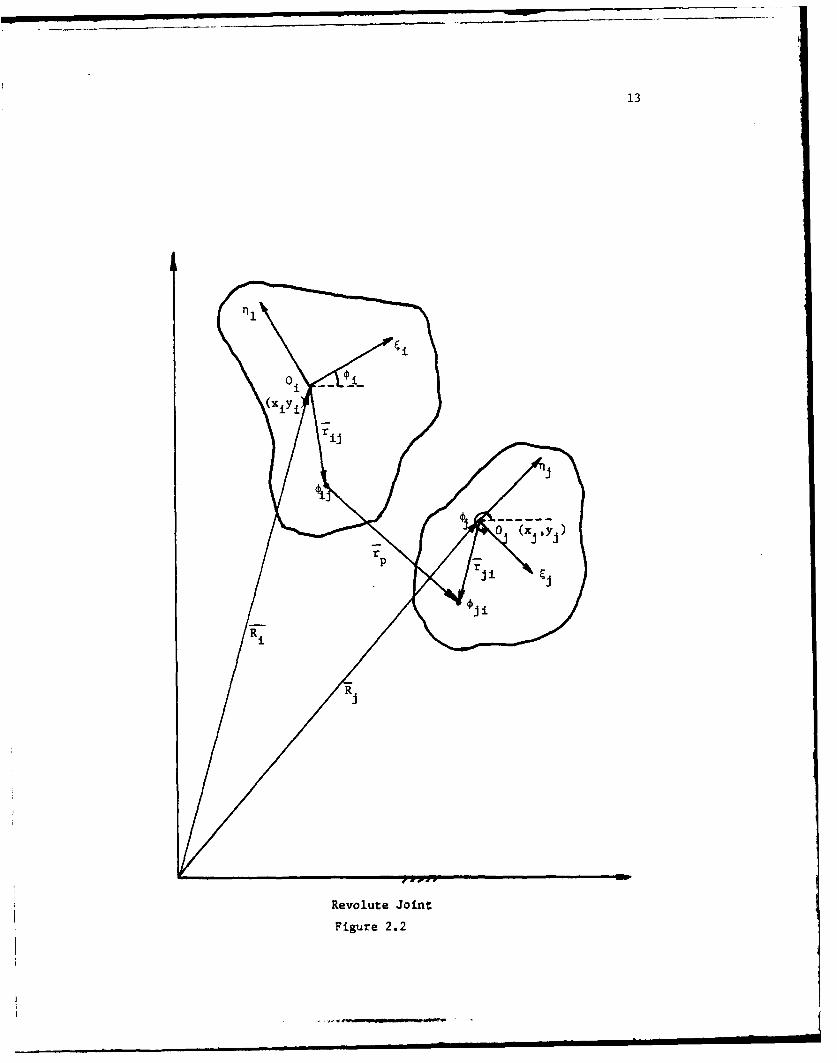
2.4 Equations of Constraint:
Figure 2.2 depicts two adjacent bodies i and J. The origins of their
body fixed coordinate systems are located by the vectors Ri and R with
respect to the inertial frame of reference. Let an arbitrary point Pij
on body i be located by rij and pJi on body j be located by rji. These
points are, in turn, connected by a vector r . One can write a vectorp
equation beginning at the origin of the inertial reference frame and closing
there, to obtain the vector relationship:
R ri+ r r - ri -R -0 (2.4.1)
The constraint equations for a revolute joint are now obtained by
requiring that pij and pji coincide. Setting rp = 0 and writing Eq. 2.4.1 in
component form, one has
xi + ij cos i - 1ij sin i - xj - cji Cos j + nji sin j . 0 (2.4.2)
Yi + i sin i + n ij cos i - Y - ji sin j - nji cos * - 0
For a translational joint shown in Figure 2.3, let points piJ and Pji
lie on some line parallel to the path of relative motion between two bodies.
In addition, let them be located such that rij and rji are perpendicular to
this line and of nonzero magnitude. Successively forming the dot product of
Eq. 2.4.1 with rij and ri and adding, one obtains the scalar equation
- rij " rji + ri +i - jij ii + rji
- 0 (2.4.3)
which reduces to
(ij cos i - nij sin i + &Ji cos -ji sin 0j)(x i - x )
+ (i sin i + ij cos i + Ji sin c.+ nJi Cos -J)(Yi - J
22 (2.4.4)i Ji -Ji
13
0 1 1
r i
r
jp rr
r
Revolute Joint
Figure 2.2

14
Y
S \\Line of relative motion01 -between bodies
x
Translational Joint
Figure 2.3

15
A second scalar equation is obtained by noting that rijx rj = 0. Expansion
of the cross product yields only a z component, which must be zero. This is
ij Cos 0 - nij sin 0i)( ji sin j + r)ji cos 01)
- (Cji cos j - nji sin 4j)( ij sin $i + nii cos = 0 (2.4.5)
Spring-Dampers: Since springs and dampers generally appear in
pairs, they are incorporated into a single set of equations. If one or the
other is absent, its effect is eliminated by setting that term to zero. The
equations for spring-damper force and torque are
-- = [ki.£Z. -to ) + V + F0 - R (2.4.6)
Tij ij I ij sij
Tij kr ij 0ij rO) + C r i . ij + T 0.j (2.4.7)
where
TF.. is the resultant force vector [Fi, Fi] in the spring-1] x ij yij
damper
R is the vector CZij cos a, .ij sin a]T between points Sij andsij i ii
Sji of a spring-damper connection on the two bodies, as in
Fig. 2.4
Tij is the torque acting on two bodies at a revolute joint
kij and k are elastic spring coefficientsrij
cij and c are damping coefficientsrij
Z0i j and 4O)j are the undeformed spring length and angular rotation
in the revolute
£iJ and )iJ are the deformed spring length and the angular rotation
in the revolute, and vij and $iJ are the time derivatives of
ij and 0iJ

16
y
0x
Liea prng ame an Atuto
Fie
osj
RI
x
Linear Spring, Damper and Actuator
Figure 2.4

17
F0i j and T are constant forces and torques applied along the
spring and around the revolute joint between two bodies
irom Figure 2.4, a vector expression similar to Eq. 2.4.1 is written as
R.+ + -r -R. =01 s.. 5.. s.. J
or in component form
Z.. C s x Cs 9 sinsc s __
(248
ijs sin ue t sin bno + tinj Cos
L xj j - s
= (xi - Cos r)+ sin ix + cs.sij ij
Y si sin + Cos (2.4.8)
where a is the angle between R s and the inertial x axis. Equation 2.4.8
ijis used to obtain Zij by noting that
z ij = NZ ij Cos a) 2+ (z ij sin a) 2] /2
= [(-xi i c os + n sin + x + Cos- s sij2+ (_ Yi - in si - i os
1s ji si + yi s ij si1s ijCo
Fy + sin j+ ] (2.4.9)
sjjIi
nsjj
Substituting the left side of Eq. 2.4.8 into Eq. 2.4.6 the following force
expressions are obtained
F xi= -I ijl Cos a (2.4.10)
F "i IF ij I sin a (2.4.11)
where cos a and sin a are obtained by dividing Eq. 2.4.8 by Zi " Finally,
defining
v - Zij (2.4.12)
...... ... .. .. . .. ..... .... .. ... .. .. .. i. . . .i im

18
and transfering Ilj, Fxij , Fyij, and vjj to the right hand sides of Eqs.
2.4.9 and 2.4.12, one obtains equations in the form required by the numerical
integration algorithm.

19
CHAPTER 3
Proposed Method of Analysis
There exist two broad categories of analysis, for which the methods
of solutions are radically different. These are:
(a) kinematically driven systems.
(b) force driven systems.
In a kinematically driven system, the input is a kinematic relationship
that, with the equations of constraint, specifies q. For instance, a
particular generalized coordinate specified as a function of time could
constitute a kinematic input. As time varies, the function changes its
value. Thus, the system assumes a new configuration. In such a system,
one assumes implicitly that the forces necessary to effect such an input
are available.
In such a system, as will be demonstrated later, the equations of
equilibrium and equations of constraint are completely decoupled and the
generalized coordinates can be computed directly from the constraint equations.
Once these have been computed, velocities, accelerations, and Lagrange
Multipliers can be computed algebraically.
In a force driven system, forces are used as inputs. Since the effect
of these forces on the generalized coordinates are not known a priori, the
equations of equilibrium are coupled with the constraint equations so that
they have to be solved simultaneously to yield the Lagrange Multipliers and
the state variables.
Analysis of Kinematically-Determined Systems
3.1 Solution for State Variables:
The analysis scheme presented here is valid for kinematically determinate
systems only. For a system with n bodies and m joints, one may write 2m

20
equations of constraint from equations (2.4.2), (2.4.4), and (2.4.5).
There are, thus
f = 3n - 2m (3.1.1)
kinematic degrees of freedom, since the constraint equations are independent.
3nDenoting the generalized coordinates by the vector q, q e R , one has the
vector of constraint equations
( R 2m
i(q)=Oi
In kinematic analysis, one may specify Z relationships among the
generalized coordinates, in terms of an input parameter a
Thus, one has X additional independent constraints of the form
2(q , a) - 0, t2 E RZ (3.1.2)
Since for a kinematically determinate system,
I + 2m = 3n
one has a situation in which the number of equations is exactly equal to
the number of variables. Quite often, the parameter a is scalar time.
Crank-Rocker Mechanism
Figure 3.1
As an illustration, consider the 4-bar crank-rocker mechanism shown
in Figure 3.10 that is used as the oscillating mechanism in fans. It consists

21
of 4 bodies, 4 revolute joints and one input relationship
2 = 02(1) (3.1.3)
Body 1 is fixed to the Newtonian Reference Frame.
Number of generalized coordinates = 4 x 3 = 12
Number of constraints due to joints = 4 x 2 - 8
Number of constraints introduced by fixing body 1 = 3
Number of input relationships = i
The input relationship can be thought of as a constraint, since it
actually constrains the rotation of body 2. Thus, one has 12 variables and
12 constraints involving the variables. There is here one input parameter
that can be varied continuously to change the configuration of the system.R3n
Letting the vector 0 E R represent the composite set of equations,
one can write
(q,a) = (3.1.4)
From the implicit function theorem of calculus, the matrix
aq kj 3n x 3n
is required to be non-singular for a solution to exist.
The set of 3n equations (3.1.4) is solved by the Newton Raphson for q,
i ionce a is fixed. Given an initial estimate q , it is required to find Aq
such that qi+l , qi + Aq is a better approximate solution of equation (3.1.4),
written now as
4 (qi+l a*) . 0 (3.1.5)
the asterisk being a reminder that the value of a is fixed.

22
From th2 Taylor expansion of (3.1.5), upto first order, one has
Ii(qi+l a*) = *(qi, ,) + 3 q = 0 (3.1.6)
or
( ( q *) Aqi = - O(qi*) ( .I.7)
i
This equation is linear in Aq and can be conveniently solved by using an
LU factorization scheme. Let
( (q , i)~-LUTherefore,
(L)(U)Aqi = - (q , a*) (3.1.8)
Let
(U) Aq1 = V, v E R3n (3.1.9)
Then,
iLv - - 4(q , a*) (3.1.10)
The vector v can be easily determined by a forward substitution procedure.i
Replacing the computed values for v in (3.1.9), Aq is computed by a back-i+l
ward substitution and the new estimate q is found. This iterationi
process is repeated until Aq satisfies the error tolerance specified.
3.2 Computation of Velocities:
The input parameter a may be related to time, and in some cases it may be time
itself. In such a case, the generalized velocity can be easily computed.
Differentiating the constraint equations (3.1.4) with respect to time,
one has
+ ( 0. (3.2.1)

23
3nwhere (//3q) E R The first 2m terms of (ao/at) are always zero, since
joint constraints are scheleronomic.
The L and U factors of (P/3q) were determined while solving for q,
so all that needs to be done in computing q is forward and backward sub-
stitutions, with a different right hand side.
3.3 Computation of Accelerations:
Differentiating equation (3.2.1) with respect to time, with q = q(t)
known at each time, in a fixed grid, one obtains
a + + + * + -0 (3.3.1)
or
()q 2 + tI ++ "+1 a Aq~ + a2- 0 (3.3.2)q~ -It~ a \q 2aat
Rearranging (3.3.2), one has
+q 2 + ~2 2 (333Dqat 2 ,aq 2Once again, by a backward and forward substitution, q can be easily
determined using the L and U factors of (3 /Dq) which are already known.
3.4 Computation of the Lagrange Multipliers:
At this stage, the information available includes the present values of
q, q, and q. Rearranging (2.1.5), one has
2m xj + 2KE -d (KE) ,i-l.3
D q1 i a dt M
- . .. R3n (3.4.1)g(Q,q,q,q), g £ R341

24
In matrix notation, (3.4.1) simplifies to
A~ ) - g(Q~q9;4q) (3.4.2)
Since (30/aq) = LU, one notes that
(0 T (OT = TLT (3.4.3)
Since L and U are known, LT and UT are also known and thus (3.4.2), which is
linear in X, can be solved to give the Lagrange Multipliers.
3.5 Analysis of Systems with Springs, Dampers and Actuator Forces:
Inclusion of springs, dampers and actuator forces in a kinematically
driven system does not pose any additional computational problems. Since
the values of the state variables q, q, and 4 are governed completely by
the constraint equations, they are obviously not affected by the inclusion
of springs and dampers. The Lagrange Multipliers, however, do change with
the inclusion of springs and actuators, since they introduce internal forces
into the system.
Since one already knows the state variables before computing the Lagrange
Multipliers, the forces due to springs, dampers, and actuators can be
computed for each analysis step. Referring specifically to (3.4.1), the
Qi' which originally might have consisted of constant forces, now become
functions of the state variables. Thus, only Q in the right hand side of
(3.4.1) needs to be modified to include spring-damper effects. The computa-
tional procedure need not change at all.

25
CHAPTER 4
Equilibrium in Force Driven Systems
The analysis of forced driven systems essentially follcws the same
procedure as transient dynamic analysis. Since the effect of the force
inputs on the generalized coordinates cannot be determined without solving
the equilibrium equations, the system of constraint equations and equili-
brium equations are coupled and must be solved simultaneously.
However, there is one major difference in the procedures adopted for
transient dynamic analysis and for equilibrium of force driven kinematic
anlysis. The difference is that there are no differential equations to
solve in the equilibrium problem. In kinematic analysis, one assumes that
initial forces and velocity effects are negligible; hence, the equilibrium
equations are algebraic. This in itself may seem to be only an academic
difference, but the fact is that the numerical algorithm becomes much
more stable and efficient. This is because a system of simultaneous alge-
braic and differential equations tends to behave like a set of stiff differential
equations. Because of this, the integration algorithm is forced to take small
time steps to obtain convergence of the solution in each period of time.
Once the inertial and velocity effects are removed the apparent stiff-
ness disappears, because what remains is an algebraic nonlinear set of equations.
Springs and dampers must, however, be treated differently in this
formulation, as compared to a kinematically driven system. The effect of
springs and dampers are not known a priori, since the state variables and
Lagrange Multipliers are computed simultaneously. One possible way to
alleviate this problem is to define each spring force as a generalized
coordinate. Corresponding to each spring force, a 'constraint' equation

26
defining it in terms of the other generalized coordinates, is added to the
Jacobian matrix.
In the method presented here, the equations of equilibrium are modified
to include the yet undetermined effects of the spring forces, and during the
Newton iterations all state variables and unknown multipliers are simul-
taneously computed.
Neglecting inertial and velocity effects from (2.1.5), one has the
equilibrium equations
j. Q i-l...3n (4.1.1)
the Qi representing all external forces as well as the internal forces
generated by springs and actuator forces. Since velocity effects are
neglected, dampers are not considered in this formulation.
Equations (4.1.1) must be solved in conjunction with the constraint
equations
4(q) - 0 (4.1.2)
Equation (4.1.1) is linear in the Lagrange multipliers, but both
equations (4.1.1) and (4.1.2) are nonlinear in the generalized coordinate
q, hence, an iterative technique is needed to obtain a solution of the
system of algebraic equations. Once again, the Newton-Raphson iteration
scheme is used. At each analysis step of this iteration scheme, one solves
a linearized version of equations (4.1.1) and (4.1.2). Linearizing these
equations, one obtains
(- [(q (,TA)- Q))iqix1i(4.1.3)

27
and
3q /q~~=-(
Rewriting equations (4.1.3) and (4.1.4) in a compact matrix form, one
has
(2OT) T. A IJ
i)T - Q (4.1.5)q L q
-O(q )i
i-I- i i
q = q + Aq
Si+l=X i + AX / (4.1.6)
Using an initial estimate of the q's and A's, one solves equation (4.1.5)
to obtain the optimal increments in the variables and substitutes them into
(4.1.6) to generate the updated values. Iterations are continued by solving
(4.1.5) again and the whole process is repeated until AA and Aq satisfy
error tolerances.
In the actual computational method used in the program, the matrix of
equation (4.1.5) is not evaluated at each step. Several iterations are done
using the same matrix but with an updated right hand side, before the values
of the entries are changed.
While this may decrease the rate of convergence to some extent, the
savings in cost realized by not re-evaluating the matrix is large enough to
offset the expenses due to increased number of iterations.

28
CHAPTER 5
Organization of the Computer Code
The DADS-2D code essentially consists of a set of subroutines,
each of which performs a specific function. The program is thus modularized
so as to make it as general as possible and, at the same time, make it
amenable to modifications.
As input to the program, the following details have to be supplied:
(a) System Parameters: amount of diagnostic information to be printed,
error tolerances, time of simulation, the a grid interval, and the system of
units to be used.
(b) Initial Estimates: of the x, y, and 0 coordinates of each body
fixed frame of reference with respect to the global frame of reference.
(c) Body Information: including mass, moment of inertia about the
center of mass, and constant forces and torques acting at the body center
of mass.
(d) Joint Information: which includes the bodies connected by each joint and
the coordinates of the joint relative to the body-fixed axes on the connected bodies.
(e) Spring Information: consisting of the two bodies to which each
spring is attached, attachment points on the two bodies, spring constants
and free lengths of the springs.
In addition, provision is made to specify curves as a discrete set
of points. The program then constructs a third-order spline through these
points to generate an analytical function.
The main computational flow of the program is shown in Figure (5.1.1)
and a detailed list of subroutines used is shown in Figure (5.1.2). A
detailed list of the various subroutines used and a brief explanation of
their functions is listed below.

29
n S-2D
Read input data
Develope row & column pointers for std. joints
Develope row & column pointers for non-std constraints]
4;o
Pefrm forward-backward subtttos
pdate Statze etre
9 No
Figure 5.1.1 Flow Chart of Computer Code
. ....... ... . ............ .. . . = 1

30
Figure 5.1.1 Print esultsi
(continued)

31
C C
z cc-4 4
U) 4~ 0 -w
0N ZN C
w4 E-I
C4-
w ONJ 00 00 (N o)w -4 vq -4i (NI u
> 1- 0 z z U) U4~E- PQ -l E-4
C-1 CN) C~4 C14 C14 (a - E-44: 'A- (N 0 0 n W) U
0 0 0 0 -~ E- z Nz z z Z -4
04-4 -4 -4 -4 1-4 -4
X~ En' '-
-4E4-4 -4 -4 E4 E- E
z

32
SUBROUTINE FUNCTION
i) XECUTE Calculates dimensions of the main arrays
2) DADSPI Main driving subroutine. Controls the
entire program by calling the other sub-
routines
3) INDATA Secondary driving subroutine, calls all the
'SET' subroutines which read all the input
data
4) SETJT1, SETJT2, Read input data corresponding to revolute
SETJT3, SETJT4 joints (JTl), translational joint (JT2),
rev-rev joint (JT3), and rev-tran joint
(JT4), respectively
5) INDSET Secondary driving subroutine, calls all
INDX subroutines which generate the row
and column indices of the non-zero entries
in the Jacobian
6) INDXCl, INDXC2 Generate row and column pointers corres-
INDXC3, INDXC4 ponding to the constraints introduced by
Joints type 1,2,3, and 4, and also the
equations of motion
7) UINDST Generates row and column pointers for the
user supplied constraints
8) ASEMBL Corrects input data to satisfy the constraint
equations and equations of motion

33
SUBROUTINE FUNCTION
9) MFEVAL Secondary driving subroutine, calls other
MFJ... subroutines which evaluate the non-
zero entries in the Jacobian matrix
10) MFJNT1, MFJNT2 Evaluate the non-zero entries introduced
MFJNT3, MFJNT4 by the constraints due to the joint types
1,2,3, and 4.
11) UMFEVL Evaluates non-zero entries due to user
supplied constraints
12) SOLVJM Secondary driving subroutine, calls the
sparse matrix subroutines, performs forward
and backward substitutions in the Newton
Raphson iterations
13) MCl9AD, MC19BD, MA13AD Sparse matrix subroutines
MC29AD, MC29BD, MC29CD
MA3OAD
14) DFASUB The subroutine which controls all numerical
computations, checks if error criteria are
satisfied, predicts values at next time step
by extrapolation techniques, prints the results
15) EQUIL Calculates the Q vector used for solving the
Lagrange multipliers
16) SPLINE {FUNCTION} Given a set of data points, the function
calculates a cubic spline through them. In
addition, it computes its first and second
derivatives

34
CHAPTER 6
Example Problems
The purpose of this section is to demonstrate the feasibility
of the preceding method by solving example problems. Three kinematically
determinate systems are analyzed, each of increasing complexity, and
numerical results are shown. In addition, a simple force driven mechanism
was analyzed.
6.1 Sample Problem 1: Slider Crank
The slider crank has been chosen as the first example because it
incorporates all the standardized elements of the code. Body 1 is the fixed
body or 'earth'. Body 2 is the crank, body 3 is the coupler link and body
4 is the slider, which slides on a fixed guide on body 1. Crank member 2 is
given an input
42(t) --I + t/2.00
where t represents time. Attached to revolute joint RVLT2 is a torsional
spring TSl, and between bodies 4 and 1, a linear spring LSl. It is attempted
to compute the generalized coordinate and the Lagrange multipliers as functions
of time. The input data for the problem are shown in Table 6.1.1.
The simulation was done using an ITEL AS-8 computer. All computations
were done in double precision and the program was run using a WATFIV compiler.
The simulation period was 10.0 seconds and a solution was forced every 0.1
seconds. Compiling time was 3.43 seconds, execution time was 53.29 seconds,
and the total cost of the run was $18.52.

35
TS1
Slde Cak ecans
FiurT61.

36
Body Data:
Coordinates of Center of Mass
Body # z x y _ _Mass Il
1 0 0 0 0 15.0 20.0
2 14.14 5.0 5.0 7r/4 15.0 20.0
3 21.21 15.0 5.0 - /4 20.0 25.0
4 - 25.0 -5.0 0 5.0 2.0
Spring Data:
Spring # Spring Type Body i Body j to 60 k
1 Linear 4 1 10 - 10.5
2 Torsional 2 3 - 0.1 4.5
Joint Data:
Joint # Type Body i Body j XIJ YIJ XJI YJI
1 RVLT 1 2 0.0 0.0 - 7.071 0.0
2 RVLT 2 3 7.071 0.0 - 7.071 0.0
3 RVLT 3 4 14.14 0.0 0.0 0.0
4 TRAN 4 1 0.0 -i.0 0.0 - 6.0
Data for Slider-Crank Mechanism
Table 6.1.1

" o C C 0 0 0 C 0 0 0 0 0 0Q m~ 0 Q cz CO Q in m4 I' a' It ' .4 O - , n
rn 1 -4 C4 U, a% 00 r- O C -4 cn t- co Ln In IT.0 r- 0 .
IcS -4 C7% m' a% 0% 0N o a' 14 -T 't0 -n r- 10 0 00 C0l a'Q
qjo oo a 0 0-r 0 ON en 0 0 %0 C -0 4 I n 0 0 C M r- Cw In C IT e-, %I I I- r- % I0 I I I cI ci L -
-(U
N" cn (n en col en m ~ m ~ en m en5 m cn C C C14 C111 C% CoD 0 a a C 0 0 0 C 0 C C 0 CD0 C) 0 0 0 C
I- - F- en mO 0 0 00 -1 ON ON CO (7% C4 r- a' rI a' cl '0 000 a' 1-a 1-0 vO - C% a% 17 co co0 '.0 1- F-- C a') 00 it, %D r- 0UCO 1- '0 a' 4 '.m a 0- a' 00 r- Co -T CO 1 0 0 00 ma ON
-n a' 1. - 1-1 r-. '.0I NIt it, 1a-1 -4 -4 -4 00 A -4 -a %D -0 Q.
o 0 CD 0D 0 0 0D CD 0 C 0m 0 C 0 0 0 0 0 0
C) 0- '0 0 0n 0 0 C a O 0 '0 0 0 '0 C 0) CD a~ a' w~- P, r- 1,, 0- 00 en N cn IT It4 .4l P4 0- r, ON5 .4 C% en
oo n C0 C7 0n 0o CN C C% C C 0 0 0o CC 0 C n C T C n 0Il Il VI I IT IT Ir It en M. I I'J
4
0 CD 0a 0 0 0- -D C) -3 .- a 0 r- -a, C - CD mO a' co0 a c- a' N0 CON Nl a' C4 0 a' -1 V CN ON e
a'I F-0 m~ 1-4 - -4 a' 0 .-T N0 C0 -a r -4 C - LnS Ln O. N '.0r '00 1-a) a' '0 N% '. r a 0 C (7% 00 C '.0 Cr rI %0 0- a' U0 LnON 0
V1 .-4 -4 - 1 N " 1-4 14 14 -4 -4 N Nn 1 N e'i co 7
0
(7 1.-"UN m r4 N r4 C4 -t C4 P T L 0 N . O(7 %t'0 C4 -D C- NT C -0 N -4 '0 0- 1.0 CO 0-4 a' UI '0 -t U, '.M w
CU~~1 U, N4 '0 V4 '-4 N Nn F- - 4 C , r. 0 - - 4 0 N
- C- %0a' 0 c-4 CD a' C4 IT0 10 -4 1.4 00 - a% - F-n ND Cn %0
* 0o 0? %0 C4 O-N 0 C C0 0 C4 CT C O%0c n T DOnO -4co 9I 7 D - l IT M I4 en IT IT ITI ~ m C
-4
e a' a a' a a' as aT 0% a' a' as a% a'% CA' a' a a% ON a' a' a'
ca LA U, U, U, U, in U,% Ul LA U,) U, U, U, U, M U, U, U, U, W) U,
'- 1- C UN I' 0 N1 U, F-- C S N n U, C-. 0 N U C-- 0' CN U, r.
.e.~~c 04 c4 4- v-4 NA N - - -S FSA a - , U ,
(U uaU) 0 U, 0 LM 0 U, 0 U, WN U, 0 , U,) LM, 0 I-' 0 U
-4 WS S * * * . * . . .0.~'C4 A 0z oz - - t ~ U , '~ ' s - O C ' a

38
"BcmX 02 BOO1 0'EcT 02 9002 1"IOMPHI 02 1003 2; Jxcc 02 R004 3 4 7 8'11CC 02 9005 5 6 9 AFALPHA 02 RC06 B C F G'IXTIL 02 R007 D E H I1TVEL 02 O08 3 K N C'ONIGI 02 B009 L PQ:l VlX 03 9010 V V 9 S'IEQY 03 B011 I Y T UIQRPUI 03 BC12 z
Figure 6.1.2: Matrix of First Derivativesof the Constraint Equation

39
The rows of the matrix of Fig. 6.1.2 represent constraints as follows:
RO01, R002 and R003 are constraints obtained by fixing body 1.
R004 and R005 are constraints obtained due to RVLT1.
R006 and R007 are constraints obtained due to RVLT2.
R008 and R009 are constraints obtained due to RVLT3.
R010 and ROll are constraints obtained due to TRANi.
R012 is the kinematic constraint imposed on the rotation of the body 2.
Each of the columns represents a generalized coordinate.
Thus, element (8,7) : J in Fig. 6.1.2 represents the partial derivative
of R008 with respect to X3, i.e., the partial derivative of the first constraint
due to RVLT3, with respect to X3 .
6.2 Example Problem 2: Peaucellier Lipkin Exact Straight Line Mechanism
Figure 6.2.1 is a schematic diagram of the Peaucellier Lipkin Exact Straight
Line Mechanism. There are B bodies in this mechanism and 10 revolute joints.
The lengths of the links comply with the conditions:
AC = CB = BF = AF - a
DF = DC - b
EA = ED = C
The mechanism always satisfies the condition2 -2 R2
(DA)(BD) = a 2 b 2 R
where R is an inversion constan.
Body 1 is ground. Crank link 2 rotates about the fixed axis E. The
motion of the crank link 2 is given as,
2 (t) - (t/loo.0o)
where t represents time. Point B of the mechanism translates along a vertical
line q-q which is always at a distance
h s
2(AE)
from point D.

40
Body 3 Body 5
RVLT3 Body 1
Figure 6.2.1: Peaucellier Lipkin Mechanism

41
BODY DATA
Body # Length Xcg Ycg cg Mass M. Inertia
1 5.0 0.0 0.0 0.0 0.0 0.0
2 5.0 -2.5 0.0 0.0 10.0 10.0
3 14.14 0.0 5.0 7r/4 10.0 10.0
4 14.14 0.0 -5.0 -ir/4 10.0 10.0
5 10.00 5.0 5.0 0.0 10.0 10.0
6 10.0 5.0 -5.0 0.0 10.0 10.0
7 14.14 15.0 0.0 -n/4 10.0 10.0
8 14.14 10.0 -5.0 r/4 10.0 10.0
JOINT DATA
Joint # Joint Type Body i Body j X1J YIJ XJI YJI
1 RVLT 1 2 0.0 0.0 2.50 0.0
2 RVLT 2 3 -2.5 0.0 -7.071 0.0
3 RVLT 2 4 -2.5 0.0 -7.071 0.0
4 RVLT 3 5 7.071 0.0 -5.00 0.00
5 RVLT 3 7 7.071 0.0 -14.142 0.00
6 RVLT 5 1 -5.00 0.00 5.00 0.00
7 RVLT 6 1 5.00 0.00 5.00 0.00
8 RVLT 4 6 7.071 0.00 -5.00 0.00
9 RVLT 4 8 7.071 0.00 -7.071 0.00
10 RVLT 7 8 0.00 0.00 7.071 0.00
TABLE 6.2.1: Data for Peaucellier Lipkin Mechanism

42
C1 (1 Nl C1 Nq q CN N -N 1 N q C1 N l N n cn cnNq C10 0 0 a 0 0 0 0 0 0 0 0 0 0 0 0 0cn in m 0 m 0 a a aIT 0 r a %N C14 c 7 0 0 0 en C1N en C70% IJM '0 -4 0
Nl M~ N~ IT IT en N1 M 0 N1 Ln U, -4 U'n c7A 0 -4 e% V)m Ln 14 ell '.0 .- N 4 4 C1 N ea -T 'D r. LM ~ 4 4 14 -4
o n 0 0 n 0 n 0 0 C4 0 0 en M 0T 00 0 0 0 0 0%
C~ Nn -4 0% C.0 Ul a% -t -- 0S 'T co m t- C% f%.0 '0 n -4 00 %0 cn -4 00 0 c 0 r3 a, co n 0 00 '.0 0
8- 0%. N . '0 '.0 '.0 '. UN '0 LA LM -n Ln C* -rn U
ro Cn 0 0- 0 0 0 0 0 0 0- n 0N 0 \0 0, 0 0 01
V) U c 0 Ln --4 ,-4 cli co Nn NN ON ID U, M.- 4 a~ '.0 .-4 03 0 3 C1 -M 00 0% %0 '.0 C14 U 0 N
> 0 0 0 0 -I - 4 -4 N4 N4 N4 N4 4 4 -4 -c
a C
o00000 0 0 0 0 0 0 a 0 0 0 0 0 0 0
-4 -q - -f r- 1-4 .-4 14 4
- -4 -4 _ -4 .4 a-4 ,- -4 -4
03 'T U, C r- ON U, -- T ON t 0 0 -4 '.0 ( n i l a, %o In ON cn U, N. 0% 0 0, 0n -4 00 c" co CC r 3 N ,
LU$ r, 0% 1-4 -.T '. 00 0 cn tA r, 030 N -q I LnI N 03 0 -4 N1.9. In Ln '0 '.0 %0 '.0 r, N. N. r, r- 00 00 00 00 co 03 % cs 0%
M% en cn- n e n Cj -4 n O o acLM 0 U, 0 Ul 0 U,% 0 , 17 % I.T 03 m~ r, NN M. %wt 0 .0 rn i-1 00 .0 en -4 00 0 en' 0 00 '.0 en 0 00 U,) N 0
e- . N . N. r- '.0 '0 '.0 '.0 U, '0 U, U, -It It IT - n en' en m
oA a 0 l 0 L0 N 0 0n 0 in0 0 0n 0 0 0 0n 0 0M 0 0
4 I4 I eI I I VI I 0I 0I 0! I I I

43
At joints A, C, D, and F, three links are connected by a single revolute
joint. The simulation is done by specifying two revolute joints at the same
point in space, connecting the three bodies. Any revolute joint can be used
to connect any two bodies, as long as one avoids having the same two bodies
attached by the two revolute joints.
In the simulation model, the center of mass of link 7 is located at point
B. Thus, when crank link 2 turns, one would expect the x-coodinate of link 7
to remain constant. The simulation results indeed show the above to be true.
The input data for the problem is shown in Table 6.2.1. The simulation
period for this model was 10.0 seconds and a solution was forced every 0.1
seconds. Compiling time was 3.44 seconds and execution time was 25.25 seconds.
All computations were done in double precision using a WATFIV compiler and an
ITEL-AS-8 computer.
6.3 Example Problem 3: Link Gear Multiplier Mechanism
Figure 6.3.1 is a schematic diagram of a Link Gear Multiplier Mechanism. This
is a three degrees-of-freedom model. When three inputs are prescribed (through
bodies 3, 11 and 12), the output of link 6 is a product of the inputs.
There are 8 bodies, 1 revolute joint, and 10 translational joints in the
mechanism. Slotted link 4 turns about the fixed axis A. Links 2, 3, 11, and
12 slide on fixed guides in body 1, and have slots in them for connections with
bodies 5 and 12. When inputs Y 3 (t), yll(t), and x2 (t) are specified, the
system responds with the motion
x6(t) - Y 3(t) xl2(t/Yl11t)
Bodies 4 and 2 can turn with respect to the pin 5. Similarly, bodies 12
and 4 turn with respect to pin 8. To model this mechanism with standard elements,
fictitious bodies 6, 7, 9, and 10 have been introduced. Bodies 5 and 6, 6
and 7, 8 and 9, 9 and 10 are connected by revolute joints. Body 5 slides along

44
Body 12
Body 4
Body 3
FBody 5
7 ABody 2
Body 1
I Figure 6.3.1: Link Gear Multiplier

45
INPUT DATA
BODY DATA
Body # Length Xcg Ycg cg Mass M. Inertia
I - 0 0 0 10.00 20.00
2 - 10.00 2.00 0.00 10.00 20.00
3 - - 2.00 10.00 0.00 10.00 20.00
4 - 5.00 5.00 0.7854 10.00 20.00
5 - 10.00 10.00 0.00 10.00 20.00
6 - 10.00 10.00 0.7854 10.00 20.00
7 - 10.00 10.00 0.00 10.00 20.00
8 - 20.00 20.00 0.00 10.00 20.00
9 - 20.00 20.00 0.7854 10.00 20.00
10 - 20.00 20.00 0.00 10.00 20.00
11 - 5.00 20.00 0.00 10.00 20.00
12 - 20.00 30.00 0.00 10.00 20.00
JOINT DATA
Type Joint # Body I Body J XIJ YIJ XJI YJI
RVLT 1 1 4 0.0 0.0 -7.071 0.0
RVLT 2 5 6 0.0 0.0 0.0 0.0
RVLT 3 6 7 0.0 0.0 0.0 0.0
RVLT 4 8 9 0.0 0.0 0.0 0.0
RVLT 5 9 10 0.0 0.0 0.0 0.0
TRAN 6 1 2 0.0 1.8 0.0 -1.0
TRAN 7 1 3 -1.0 0.0 1.0 0.0
TRAN 8 1 11 2.5 0.0 -2.5 0.0
TRAN 9 1 12 0.0 25.0 0.0 -5.0
TRAN 10 3 5 0.0 - 1.0 0.0 -1.0
TRAN 11 4 6 0.0 1.0 0.0 1.0
TRAN 12 2 7 4.0 0.0 4.0 0.0
TRAN 13 11 8 0.0 - 1.0 0.0 -1.0
TRAN 14 4 9 0.0 1.0 0.0 1.0
TRAN 15 12 10 1.0 0.0 1.0 0.0
Data for Link Gear Multiplier
TABLE 6.3.1

46
en Ln I~ 1-4 %0 m m a, 10 0% 0% m -n Co 0% IT 1f r- fn rLn 1-4 - - en 0 0 0 en -t 0T 00 m .0 0 --T co C4 LM a00 % 0% 0 0D -f - (Ni mN cn IT .t LM Ln U, U 0 '.0 '. p
0- 0- 0- 0000 0 0 0 0 0 c 00 0 o 0 0 0 0 0 0 00
-4-4 -4 r-4 -4 -4- -4 - -4 -4 -4 -40 0 0 0 0D 0 1-4 -4 -4 0 0 0D 0 -4 0 14 0 0
-4 1-4 i m 0 0 0 0 0 0) g 0a U, 0 '- I- r.. 0% C14 Q 0n 0 -4 M 0% Pm0
'0 0 ~-4 en " IT 00 LO U, p n U, 00 M 0% '.0 U, ID C. % "N>' 0 0 '0 1-4 CN M' -:T 'o 00 0 C4 -.T e- a,. ( Ui 00 1-4 IT co
o o 0 0 0 0 0 0 -4 1-4 '-4 --1 -4 C14 (N en4 mo a 0 0 a 0 0 0D 0 0 0 0 0 0 0 0
- -4 -4 - 4 - 4 - 4r 4 - 4 -4 4 -4 - 4 -
-4 -4,-4 r-4 r-4 r-4 ,-I ,-4 1.4 -4 ,-q 1-4 - 4 4 -4 0 .-4 14 -4 -4 '-4a 0 0 0 0D 0 0 0 0 0 0D 0 0 0z 0 0 0 0 0=.--. 0 Q p p cz lz 9z p %0 0
CD 0 in 0 -4 ('- P. 0% (N en 8 0 1- r 0 0% -4 %.?aN 0 -. Q en0 C1 IT -t Ln U eni L 00 cn 0% '.0 u, U, %D0 % (
-4 0 0 -4 C14 rn IT '.0 co 0 Nq .7 P 0% ul U 0 O 4 IT 00a 0a -4 '-4 -1 '-4 '-4 eq (N N (n (nCD00 0 0 0 0 0 0 0 0 0 0D 0 0 0 0
-4 -4 r-4 -4 4 -4 -4 -4 -4 -4 - -4 -4 -4 r- r-4 -4 -4 (NO 1 4 '-4 0 0 0 0 0 0 0 0 00 0 0 0 0 0 00 0 gz c 0
-4 0 0 00C 0 0 0 0 0 0 0 0 0D 0r-4 0 0 0a 0 0 0 0 0 0 08 0 0D CI. .0> 0 n a, Lt4 0 U, 0 ui 0 U, 0 U,) 0 U, 0 ) U, 0 , 0o 1. '-4 (N (N m cn --T IT U, U, '.0 '.0 I- r- 00 00 a% a, W~
-4 4 C4 -4 -4 -4 -4 - 4 -4 -4 -4 -4 4 -4 -4 -4 -4 -4 4
o 0 00 0 0 0 0 0 0 0 14 0 0 0 0 0 0 -4
-4 n U, 0n U, 0n U, 0M U, 0 U , 0 U, 0 U , 0 U'< CD ( U r-. 0 (N4 U, r- 0 , Ln f 0%(N U, 9- 0 4 ( M U,
o q o * 0 4 0 1 C4 4 C14 (N 4 (N (N (N 04 .~ .' .~ .~- 7
-4 4 -4-4 -4I -4 1 -4 -4 r -4 f -4 -4 -4 14 -4 4 -4 -4 -4a 0C 0 0 0 0 0 0 0 0 0 0 0 0 0 0 -4 0 0 0
9z Q z z9 0 0 :m 0 0 0 0 0L 0 , L , U 0 U, 0 U, 0 U, 0 Ui 0 U, o U 0 U,
>' 0M (N Uin.0 ( U r- 0 eq U, r- 0 CN U, r. 0 4 (N U, -o -4 (q U, '. 0 r- 00 0 -4 (N cn U, '0 Ps co 0 -4 (N (no o 0 0 0D 0 0 0 -44 -4 4 -4 .- . 4 -4 (N (N (N (
-4 -4 -4 4 -4 -4 -44 -4 -4 -4 -4 -4 -4 -4 -4 -4 -4 -

47
body 3, body 6 slides on body 4 and body 7 slides on body 2. Similarly,
body 8 slides on body 11, body 9 slides on body 4, and body 10 slides on
body 12.
The model used for simulation thus has 12 bodies, 5 revolute joints and
10 translational joints. The dimensions of the mechanism may be arbitrary,
provided the topological configuration does not change. The input data for
the problem are shown in Table 6.3.1.
Table 6.3.2 contains results of the simulation. Columns 2, 3, and 4
contain the values Y3, X12, and Yll, respectively. Using these values, the
expected value of X6 is computed and printed in column 5. Column 6 contains
the actual value of X6, as obtained from the simulation.
The simulation period for the job was 10.0 seconds, with a solution
being forced every 0.10 seconds. All computations were done using a WATFIV
compiler, on an ITEL AS-8 computer. Compilation time was 3.51 seconds, and
execution time 32.46 seconds. Total cost of the job was $20.79.
6.4 Example Problem 4: Force driven 4-bar linkage
Figure 6.4.1 is a schematic figure of a 4-bar linkage, which has one
degree-of-freedom. The mechanism is initially in a non-equilibrium position.
The problem at hand is to find the equilibrium position of the mechanism when
it is subject to its own body forces.
Pertinent input data are shown in Table 6.4.1. The values of the general-
ized coordinates and the Lagrange multipliers at equilibrium position are
computed.
It must be noted that for the force driven case, the program attempts
to find an equilibrium position if such a position exists at all. Thus,
there is no parameter like time, as in analysis of kinematically determinate
systems.

48
BODY DATA
Body # Length Xcm Ycm 0cm Mass MI
1 100 0.0 -0004 0.0 0.0 0.0
2 100 8.682 -49.240 -1.3962 1.0 1.0
3 100 67.36 -98.480 0.0 1.0 1.0
4 100 108.682 -49.24 -1.3962 1.0 1.0
JOINT DATA
Joint # Joint Type Body I Body J X1J YIJ XJI YJI
1 RVLT 1 2 0.0 0.0 -50.0 0.0
2 RVT 2 3 50.0 0.0 -50.0 0.0
3 RVLT 3 4 50.0 0.0 -50.0 0.0
4 RVLT 4 1 50.0 0.0 -50.0 0.0
Data for Four-bar Linkage
Table 6.4.1

49
RESULTS
Estimates obtained using €2 = const. - -1.3962 rads
Body # X Y (Rads)
1 10 - 1 4 0 0
2 8.68553 -49.2398 -1.3962
3 67.3711 -98.479 10-14
4 108.6855 -49.2398 1.7453
Estimates of Lagrange Multipliers
JT # Ax Xy
1 45.40 386.08
2 45.40 128.69
3 45.40 -128.69
4 45.40 -386.08
Constraint
002 - 10 " 0 8942.34
(Moment)
Execution time - 0.51 secs. in the ITEL AS-8 Computer
# of iterations - 2
Table 6.4.2

50
FINAL RESULTS
Generalized Co-ordinations
Body # x Y O(Rads)
1 0 0 0
2 10- 14 -50.00 -1.5708
3 50.00 -100.00 0"17
4 100.00 - 50.00 1.5708
Lagrange Multipliers
Joint # Xx Ay
1 10- 13 386.08
2 10- 13 128.696
3 10- 1 3 -128.696
4 10- 1 3 -386.088
CPU Time - 1.02 secs
# of iterations - 2
Table 6.4.3

51.
, RVLTl Zledj i ILT
I' 3od".3
RVLT2 RVLT3
Figure 6.4.1: Pour Bar Linkage

52
The solution strategy for force driven mechanisms is slightly different
from what has been explained in the previous examples. The program has been
coded such that all Lagrange multipliers have zero initial estimates. During
subsequent iterations for closure of the mechanism, these estimates are
expected to reach the correct values.
The difficulty with this strategy is that very often the Jacobian
matrix of first derivatives does not have full row rank especially when all
Lagrange multipliers have zero initial estimates. To overcome the problem
caused by singularity of the matrix, the sparse matrix code fixes values for
K of the state variables arbitrarily where K is the nullity of the matrix,
and proceeds to solve for the remaining unknowns from the largest non-
singular submatrix available.
Thus, the configuration of the mechanism is changed considerably from
what was initially specified. Since the initial estimates of the dependent
variables have not changed, the input data is not a good estimate any more.
Thus while attempting loop closure, the program may need several iterations
and in some cases closure may not be attained at all. To offset this
computational difficulty, the following strategy is employed: If a mechanism
has f degrees-of-freedom, f coordinates are kept fixed by the code at their
initial estimates. Thus, one can now obtain the generalized coordinates by
solving the constraint equations. Once all the variables have been obtained,
Lagrange multipliers are computed.
The values computed above are read as initial estimates for the force
driven system. Since one has a reasonable estimate of the Lagrange multipliers
and other generalized coodinates, closure will be attained reasonably quickly.
This method may not work well for problems in which the initial estimates
are inaccurate, but for reasonably good initial estimates closure is guaranteed.

53
CHAPTER 7
Conclusions
The basic attempt in this report is to formulate and code a general
purpose method for kinematically analyzing force driven and kinematically
driven mechanisms.
It was shown that for the kinematically driven systems constraint
equations can be used to evaluate the generalized coordinates. Successive
differentiation of the constraint equations yield velocities and accelerations.
The equations of equilibrium were shown to be uncoupled from the constraint
equations, and the unknown Lagrange multipliers can be computed even after
including inertial effects. In all cases, it was shown that the coefficient
matrix is the (DO/aq) matrix or its transpose, and hence, computations of
velocities, accelerations and Lagrange multipliers are not very expensive.
It was shown that for the force driven system, the equations of equili-
brium and the constraint equations were coupled. To avoid solving the dif-
ferential equations of motion, it was assumed that inertial effects were
negligible and thus this solution technique is applicable only to kinetostatic-
quasistatic systems.
Three example problems of varying complexity were solved, and the solution
strategy was shown to be feasible. Solution of velocities and accelerations
have not been included in the present code but can be done with very few
modifications in the main program.

54
REFERENCES
1) Haug, E.J., Wehage, R., and Huang, R.C., Computational Methods in
Mechanical System Dynamics, College of Engineering, The University of
of Iowa, 1980.
2) Duff, I.S., MA-28 - A Set of Fortran Subroutines for Sparse Unsymmetric
Linear Equations, Harwell, United Kingdom Atomic Authority, July, 1972.
3) Kaufman, R.E., "Kinematic and Dynamic Design of Mechanisms " in Shock
and Vibration Computer Program Reviews and Summaries, ed. by W. & B.
Pilkey, Shock and Vibration Information Center, Naval Research Lab.,
Code 8404, Washington, D.C., 1975.
4) Paul, Burton, Kinematics and Dynamics of Planar Machinery, Prentice-
Hall, Inc., Englewood Cliffs, New Jersey, 1979.
5) Uicker, J.J., "Users' Guide for IMP: A Problem-Oriented Language
for the Computer-Aided Design and Analysis of Mechanisms," NSF Report,
Res. Grant GK-4552, University of Wisconsin, Madison, Wisc., 1973.
6) Paul, B. and Hud, G., "Users' Manual for Program Dymac-L2", MEAM
Report 76-5, Dept. of Mechanical Engg., Univ. of Pennsylvania, Phila.,1975.
7) Chace, M.A. and Smith, D.A., "DAMN-Digital Computer Program for the
Dynamic Analysis of Generalized Mechanical Systems," SAE Trans., 80,
969-983, 1971.
8) Dix, R.C. and Lehman, T .J., "Simulation of the Dynamics of Machinery,"
J. Engg. Ind. Trans., ASME Ser. B, 94, 433-438, 1972.
9) Orlandea, N., Chace, M.A. and Calahan, D.A., "A Sparsity Oriented Approach
to the Dynamic Analysis and Design of Mechanical Systems - Parts I and
II," J. Engg. Ind. Trans., ASME Ser. B, 99, 733-779, 780-784, 1977.
-. ~.I. i

55
10) Wehage, R.A., Haug, E.J., Barman, N.C., "Dynamic Analysis and
Design of Constrained Mechanical Systems," Technical Report No. 50,
Contract No. DAAK30-78-C-0096, November, 1978.
11) Langrana, N.A. and Bartel, D.L., "An Automated Method for Dynamic Analysis
of SpatialLinkages for Biomechanical Systems," J. Engg. Ind. Trans.,
ASME Ser. B, 97, 556-574, 1975.
12) Huston, R.L., Passerello, C.E. and Harlow, M.W., UCIN - Vehicle Occupant/
Crash Victim Simulation Model, Structural Mechanics Software Series,
University Press of Virginia, Charlottesville, VA, 1977.
13) Goldstein, Herbert, Classical Mechanics, Addison-Wesley Publishing
Company, Reading, Massachusetts, 1950.
-• .•-e- ~ .-.... eWCM * .%.. -~m m

V!
DISTRIBUTION LIST
Please notify USATACOM, DRSTA-ZSA, Warren, Michigan 48090, of correctionsand/or changes in address.
Commander (25) Director (01)US Army Tk-Autmv Command Defense Advanced ResearchR&D Center Projects AgencyWarren, MI 48090 1400 Wilson Boulevard
Arlington, VA 22209Superintendent (02)US Military Academy Commander (01)ATTN: Dept of Engineering US Army Combined Arms Combat
Course Director for Developments ActivityAutomotive Engineering ATTN: ATCA-CCC-S
Fort Leavenworth, KA 66027Commander (01)US Army Logistic Center Commander (01)Fort Lee, VA 23801 US Army Mobility Equipment
Research and Development CommandUS Army Research Office (02) ATTN: DRDME-RTP.O. Box 12211 Fort Belvoir, VA 22060ATTN: Dr. F. Schmiedeshoff
Dr. R. Singleton Director (02)Research Triangle Park, NC 27709 US Army Corps of Engineers
Waterways Experiment StationHQ, DA (01) P.O. Box 631ATTN: DAMA-AR Vicksburg, MS 39180
Dr. HerschnerWashington, D.C. 20310 Commander (01)
US Army Materials and MechanicsHQ, DA (01) Research CenterOffice of Dep Chief of Staff ATTN: Mr. Adachifor Rsch, Dev & Acquisition Watertown, MA 02172ATTN: DAMA-AR
Dr. Charles Church Director (03)Washington, D.C. 20310 US Army Corps of Engineers
Waterways Experiment StationHQ, DARCOM P.O. Box 6315001 Eisenhower Ave. ATTN: Mr. NuttallATTN: DRCDE Vicksburg, MS 39180
Dr. R.L. HaleyAlexandria, VA 22333 Director (04)
US Army Cold Regions Research
G Engineering LabP.O. Box 282ATTN: Dr. Freitag, Dr. W. HarrisonDr. Liston, Library
Hanover, NH 03755

President (02) Director (02)Army Armor and Engineer Board Defense Documentation CenterFort Knox, KY 40121 Cameron Station
Alexandria, VA 22314Commander (01)US Army Arctic Test Center US Marine Corps (01)APO 409 Mobility & Logistics DivisionSeattle, WA 98733 Development and Ed Command
ATTN: Mr. HicksonCommander (02) Quantico, VA 22134US Army Test & EvaluationCommand Keweenaw Field Station (01)ATTN: AMSTE-BB and AMSTE-TA Keweenaw Research CenterAberdeen Proving Ground, MD Rural Route 121005 P.O. Box 94-D
ATTN: Dr. Sung M. LeeCommander (01) Calumet, MI 49913US Army Armament Researchand Development Command Naval Ship Research & (02)ATTN: Mr. Rubin Dev CenterDover, NJ 07801 Aviation & Surface Effects Dept
Code 161Commander (01) Washington, D.C. 20034US Army Yuma Proving GroundATTN: STEYP-RPT Director (01)Yuma, AZ 85364 National Tillage Machinery Lab
Box 792Commander (01) Auburn, AL 36830US Army Natic LaboratoriesATTN: Technical Library Director (02)Natick, MA 01760 USDA Forest Service Equipment
Development CenterDirector (01) 444 East Bonita AvenueUS Army Human Engineering Lab San Dimes, CA 91773ATTN: Mr. EckelsAberdeen Proving Ground, MD Engineering Societies (01)21005 Library
345 East 47th StreetDirector (02) New York, NY 10017US Army Ballistic Research LabAberdeen Proving Ground, MD Dr. I.R. Erlich (01)21005 Dean for Research
Stevens Institute of TechnologyDirector (02) Castle Point StationUS Army Materiel Systems Hoboken, NJ 07030Analysis AgencyATTN: AMXSY-CMAberdeen Proving Ground, MD21005

Grumman Aerospace Corp (02) CALSPAN Corporation (01)
South Oyster Bay Road Box 235
ATTN: Dr. L. Karafiath Library
Mr. F. Markow 4455 Benesse Street
M/S A08/35 Buffalo, NY 14221
Bethpage, NY 11714SEM, (01)
Dr. Bruce Liljedahl (01) Forsvaretsforskningsanstalt
Agricultural Engineering Dept Avd 2
Purdue University Stockholm 80, Sweden
Lafayette, IN 46207Mr. Hedwig (02)
Mr. H.C. Hodges (01) RU 111/6
Nevada Automotive Test Center Ministry of Defense
Box 234 5300 Bonn, Germany
Carson City, NV 89701Foreign Science & Tech (01)
Mr. R.S. Wismer (01) Center
Deere & Company 220 7th Street North East
Engineering Research ATTN: AMXST-GEI
3300 River Drive Mr. Tim Nix
Moline, IL 61265 Charlottesville, VA 22901
Oregon State University (01) General Research Corp (01)
Library 7655 Old Springhouse Road
Corvallis, OR 97331 Westgate Research Park
ATTN: Mr. A. Viilu
Southwest Research Inst (01) McLean, VA 22101
8500 Culebra RoadSan Antonia, TX 78228 Commander (01)
US Army Developmant and
FMC Corporation (01) Readiness Command
Technical Library 5001 Eisenhower Avenue
P.O. Box 1201 ATTN: Dr. R.S. Wiseman
San Jose, CA 95108 Alexandria, VA 22333
Mr. J. Appelblatt (01)
Director of EngineeringCadillac Gauge CompanyP.O. Box 1027
Warren, MI 48090
Chrysler Corporation (02)
Mobility Research Laboratory,
Defense EngineeringDepartment 6100P.O. Box 751Detroit, MI 48231