1

Bilateral FDI flows, Productivity Growth and Convergence:

The North vs. The South1

Firat Demir University of Oklahoma

Department of Economics 436 CCD1, 308 Cate Center Drive Norman, Oklahoma, USA 73019

E-mail: fdemir@ou.edu

Yi Duan2 University of Oklahoma

Department of Economics Norman, Oklahoma, USA 73019

158 CCD1, 308 Cate Center Drive E-mail: yiduan@ou.edu

Conditionally Accepted at World Development

1ACKNOWLEDGMENTS: We thank Gregory Burge, Pallab Ghosh, John Harris, Daniel Hicks, Arslan

Razmi, and the session participants at the Eastern Economic Association and the Missouri Valley Economic

Association meetings in 2015 for their comments on earlier drafts of this paper. We are also thankful to the

two anonymous referees of this journal for their constructive suggestions. We thank Xiaoman Duan, Xiaokai

Li, Wenliang Ren and Ying Zhang for their excellent research assistance. Firat Demir thanks Fulbright

Commission and the Faculty of Economics at the University of Montenegro for his Fulbright visit during

2015-2016. The usual disclaimer applies.

2Corresponding author. Tel: +1 (405) 325 2861.

2

Bilateral FDI flows, Productivity Growth and Convergence:

The North vs. The South

ABSTRACT

Controlling for the aggregation bias in FDI flows and the home and host country heterogeneity within and

between Northern and Southern countries, we explore the effects of bilateral FDI flows on host country

productivity growth, and on the productivity convergence dynamics between the host and the productivity-

frontier country. Using bilateral FDI flows data from 108 host and 240 home countries over 1990-2012, and

employing a variety of estimation techniques together with a rich battery of robustness tests, we find no

significant effect of bilateral FDI flows on either host country productivity growth or on the productivity gap

between the host and the frontier country. We also show that these findings are not sensitive to the direction

of FDI flows, which are South-South, South-North, North-South or North-North. In a decomposition

exercise, we also fail to find any significant effect of bilateral or aggregate FDI flows on physical capital

growth. Yet, we find some evidence of a positive effect of FDI flows on human capital growth but just in one

direction, South-South. Last but not least, we fail to find any productivity growth or convergence effect at the

sectoral level, including agricultural, industry or services sectors.

Keywords: Bilateral FDI flows; Productivity growth, Productivity convergence; Home and host country

heterogeneity, South-South FDI

JEL Codes: F21, F43, O11, O47

3

1. INTRODUCTION

The liberalization of international capital flows has been one of the main pillars of the Washington Consensus

since the 1980s. The defenders of this consensus argued that a myriad of benefits were to be derived from

external financial liberalization, including allocation efficiency, increased credit flows, relaxation of foreign

exchange bottlenecks, risk diversification, prevention of rent seeking, higher capital accumulation and job

creation as well as technology and skills transfer, all of which were expected to enhance productivity and

economic growth. Furthermore, these effects were thought to be stronger in less developed host countries (i.e.

the South), allowing them to catch up with the developed world (i.e. the North). Thanks to the financial

liberalization wave of this period, global FDI flows increased from $54 billion in 1980 to $208 billion in 1990,

and then to $1.5 trillion in 2013. The rapid growth in FDI flows was accompanied by an increased

competition among prospective host countries. Each year between 2000 and 2013, an average of 56 countries

introduced a total of 1,440 regulatory changes in their investment regimes, 80% of which were to promote

and facilitate a more favorable environment for foreign investors. Complementing legislative changes,

bilateral investment treaties (BITs) also spiked, reaching 3,140 by 2015, 88% of which were signed after 1990

(UNCTAD, 2014). However, despite this stout pro-FDI stance across countries, and despite the fact that

technology transfer remains one of the top expectations of developing countries from FDI, the growth and

productivity effects of foreign investment have been a source intense debate in economics with the empirical

evidence being inconclusive at best so far.

In this paper, we contribute to the debate on the productivity effects of FDI by addressing two major

issues that were previously unaccounted for, which are the aggregation bias and the home and host country

heterogeneity within and between Northern and Southern countries. Most empirical work on the topic is

based on aggregate FDI flows, assuming that bilateral flows from (to) multiple country pairs are symmetrical

and homogenous. In fact, as we discuss later in our data section, FDI flows are highly dynamic and

heterogeneous with investments and divestments from different investors taking place simultaneously. They

are also likely to differ in sectoral orientation, type (i.e. merger and acquisition vs. Greenfield, horizontal vs.

vertical), duration of stay and investment size as well as managerial and operational practices, which may

4

affect the strength of vertical and horizontal linkages, and eventually the productivity spillover dynamics.

Thus, aggregating inherently heterogenic investment flows, as if they all have the same productivity effects,

causes what we refer to as the aggregation bias. A second cause of bias is the assumption that investment

flows from (to) home (host) countries with different economic development levels have homogenous

productivity effects. This is surprising given that there are strong reasons as to why the productivity effects

may differ between Northern and Southern home and host countries, including differences in endowments,

institutions, know-how, experience, technological sophistication and sectoral concentration. Differences in

consumer preferences and the absorptive capacity of host countries also affect the potential for knowledge

and technology spillovers. In other words, not all FDI is created equal. Another reason why we should pay

attention to differences between Northern and Southern FDI flows is the significant growth of FDI to and

from Southern countries, reaching 64% of global inflows and 43% of outflows in 2013 (UNCTAD, 2016).1

Furthermore, a majority of Southern FDI outflows is now directed to other Southern countries, reaching as

high as two thirds of their total in 2010 (UNCTAD, 2011; WB, 2011).

In the empirical analysis, we explore two overlapping questions: (i) what are the total factor

productivity (TFP) growth and convergence effects of bilateral FDI flows? (ii) Are the productivity effects of

FDI flows conditional on the direction of these flows, that is South-South, South-North North-South or

North-North? The empirical results, using a rich panel of bilateral FDI flows data between 108 host and 240

home countries during the period of 1990-2012 suggest that bilateral FDI inflows have no significant effect

on either host countries’ productivity growth or on the productivity gap between host countries and the

frontier country in any of the four directions. The validity of these findings is confirmed using a variety of

estimation methods and a rich battery of robustness checks. In a decomposition exercise, we also fail to find

any significant effect of bilateral or aggregate FDI flows on physical capital growth. Yet, we find some

evidence of positive effect of FDI flows on human capital growth but just in one direction, South-South. We

also fail to find any productivity growth or convergence effect at the sectoral level in agriculture, industry or

services.

5

The rest of the paper is organized as follows. Section 2 introduces the literature review. Section 3

describes the data, empirical model and estimation methodology. Section 4 presents the empirical results,

including extensions and robustness analysis. Section 5 concludes.

2. LITERATURE REVIEW

Foreign firms are shown to have higher productivity, capital intensity, technology, better risk management,

know-how, larger supply of internal finance and easier access to international goods and capital markets

(Arnold and Javorcik, 2009). However, the existing empirical evidence on FDI spillovers, using country, firm

or industry level data, has been inconclusive.2 Using firm level data, Djankov and Hoekman (2000) for Czech

Republic, Keller and Yeaple (2003) for the US, Haskel et al. (2007) and Harris and Moffat (2013) for the UK,

Fu (2008), Fu and Gong (2011) and Demir and Su (2016) for China, Arnold and Javorcik (2009) for

Indonesia, and Yasar and Paul (2009) for Turkey find evidence of positive productivity growth spillovers

from FDI. In contrast, Haddad and Harrison (1993) for Morocco, Aitken and Harrison (1999) for Venezuela,

Liu (2008) and Xu et al. (2014) for China, and Fons-Rosen et al. (2014) for firms in 25 advanced countries do

not find any significant or exogenous productivity spillovers from FDI. In fact, after controlling for the self-

selection bias (i.e. foreign investment flowing into more productive plants), Aitken and Harrison (1999)

report a significantly negative productivity effect from foreign to domestic firms. Harris and Robinson (2002)

also find evidence showing a decline in plant-level productivity after foreign firm acquisitions in the U.K. On

the macro side, Alfaro et al. (2009) fail to find any exogenous effect of FDI on aggregate TFP growth.

Building on these results, Girma et al. (2015) show that foreign ownership has a direct positive productivity

effect on foreign-owned firms but an indirect negative effect on non-foreign domestic firms in China.

While not explored before, the spillover effects of FDI may in fact be conditional on home and host

country characteristics, especially if aggregate FDI flows are heterogeneous in nature. For example, the

productivity effects of South–South flows may lag behind those of North-South flows, if, as argued by the

Neoclassical theory, Northern firms have better technology, know-how and managerial skills, better risk-

management, and have more experience to pass on to host countries. As a result, the potential for knowledge

and technology transfer between a Northern home and a Southern host country should be higher than in any

6

other directions (Schiff, et al., 2002; Schiff and Wang, 2008). In contrast, the Structuralist as well as the new

trade theory suggest that South-South FDI may carry a higher potential for technology transfer as the gap

between the home and host country technologies and endowment differences are smaller, allowing for higher

complementarity, absorptive capacity and more appropriate technology adoption in host countries (Akamatsu,

1962; Amsden, 1980, 1987; Kokko et al., 1996; De Mello, 1999; UNCTAD, 2011; Mayer-Foulkes and

Nunnenkamp, 2009; Amighini and Sanfilippo, 2014; Bahar et al., 2014; Dahi and Demir, 2016). South-South

FDI is also argued to encompass older technologies, which, in terms of production techniques and product

characteristics, are better fit for technological advancement and productivity improvement in host countries

than cutting-edge technologies from Northern investors (Stewart, 1982, 1990; Kaplinsky, 1990, 2013; Nelson

and Pack, 1999). Compared to the accumulation aspect of technological change, the assimilation aspect may

then be more important for productivity improvements as adoption of imported technologies is easier when

the technological gap is smaller and operational capabilities are closer between host and home countries. Thus,

when it comes to technology and productivity spillovers, capacity and capability are not necessarily one and

the same thing (Lall, 2000). Similarities in tastes and preferences between host and home countries within the

global South may also allow for easier technology adoption and productivity improvement while enabling

Southern multinational corporations to address local consumer needs better (UNCTAD, 2011: 42; Amighini

and Sanfilippo, 2014). Recent empirical work using case studies provide strong support for these hypotheses,

showing that developing country technologies are better fit for local needs, demand structures, market size,

factor endowments and adaptive capabilities (Atta-Ankomah, 2014; Agyei-Holmes, 2016; Xu et al., 2016).

Differences in sectoral composition of FDI are another potential source of heterogeneity within and

between Southern and Northern investment flows. While manufacturing industries are often pointed out to

be the key catalyst for productivity spillovers, the same is not true for other sectors (Lee, 2009; Rodrik, 2013).

Looking at the distribution of global Greenfield FDI flows to the South, we find that most went to services

and primary sectors, jointly accounting for 54% of the total between 2004 and 2013, while manufacturing

received the remaining 46%. In terms of total FDI stock in Latin America, more than half of FDI in 2012

was in services, and in the case of South America, once we exclude Brazil, services and primary sectors

7

accounted for more than 85% of the total FDI stock in 2012 (UNCTAD, 2014, p.63). It is possible that

South-South and North-South investment flows differ in their sectoral distributions. In the case of Africa, for

example, only 3% of intra-African Greenfield FDI flows went to primary sectors, compared to 24% of flows

from the rest of the world between 2009 and 2013. Likewise, the share of manufacturing was 48% for intra-

regional flows in Africa compared to 32% for investment flows from outside the region (UNCTAD, 2014,

p.41). The sectoral composition of FDI can also affect the convergence dynamics between the North and the

South. As manufacturing industries enjoy higher productivity convergence (Rodrik, 2013), foreign

investments that are more manufacturing oriented are more likely to facilitate convergence between the

productivity frontier and the rest. Controlling for the self-selection of foreign firms into higher productivity

firms, Demir and Su (2016) find that FDI has a positive effect on TFP levels in Chinese auto-industry.

There are also doubts as to the technology transfer potential of foreign firms, particularly those from

the North, because of their tendency to work in enclaves and to maintain proprietary ownership of

intellectual copyrights. For example, only a fraction of research and development (R&D) activities by US

majority-owned transnational companies (TNCs) are undertaken abroad, just below 16% in 2010. Of this

amount, 80% was done in Northern countries (NSF, 2014; Dahi and Demir, 2016). Furthermore, four

countries, Brazil, China, India and South Korea received 68% of the total R&D done by US TNCs in

developing countries in 2010 (NSF, 2014; Dahi and Demir, 2016). Yet, there is also no evidence that R&D

spending by Southern TNCs in host countries is any higher than their Northern counterparts. Several studies

also suggest that Southern investors have a comparative advantage in operating in institutionally less

developed and more risky countries (Aleksynska and Havrylchyk, 2013; Demir and Hu, 2016). This advantage

may help overcome the disadvantaged position of Southern investors (in technology, operational capabilities,

experience, etc.) while facilitating productivity spillovers for host countries.

3. EMPIRICAL ANALYSIS

3.1 Model Speciation and Estimation Methodology

We explore the effects of bilateral FDI flows on aggregate productivity growth using equation (1), as in

Levine et al. (2000), Bwalya (2006), Doytch and Uctum (2011), and Aghion et al. (2009):

8

𝐺𝑟𝑜𝑤𝑡ℎ!" = 𝛼! + 𝛽! ∗ 𝐹𝐷𝐼!"#!!!! + 𝛽! ∗ 𝐹𝐷𝐼!"#!!!" + 𝛽! ∗ 𝐹𝐷𝐼!"#!!!" + 𝛽! ∗ 𝐹𝐷𝐼!"#!!!! + 𝛾!𝑋!"!! +

𝛿!" + 𝛿! + 𝜀!" (1)

where 𝐺𝑟𝑜𝑤𝑡ℎ!" refers productivity growth in host country i in year t, and its measurement is

discussed in the next section. 𝛿!" and 𝛿! control for country-pair and year fixed effects, and 𝜀 is the error

term. In order to control for the lagged growth effects as well as the reverse causality problem, all control

variables are lagged by one period.3

FDIijt-1 is FDI inflows from home country j to host country i at time t-1, normalized by host country

GDPs. The normalization helps correct for size and scale differences between host economies and FDI flows.

SS, SN, NS and NN refer to the direction of FDI flows that are South-South, South-North (i.e. from

Southern home to Northern host country), North-South (i.e. from Northern home to Southern host country)

and North-North, respectively. Thus, the effect of FDI on host country productivity growth is conditional on

the direction of the flows as given by 𝛽! for South-South, 𝛽! for South-North, 𝛽! for North-South, and 𝛽!

for North-North flows. As discussed before, the expected sign and significance of these coefficients may be

conditional on the direction of FDI flows. For example, based on the neoclassical theory, North-South flows

are assumed to have a positive and more significant effect on productivity growth than South-South flows

while North-North, or South-South flows are not expected to have any significant effect given similarities in

their endowments and technology. Likewise, South-North flows should have an insignificant effect since the

South lags the North in productive capacity. On the other hand, if income, production structure,

endowments, adaptive capacities and preference similarities are more important for spillover effects, as

argued by the new trade theory and the Structuralist literature, than we would expect South-South and North-

North flows to be more conducive for TFP growth than North-South or South-North flows.

Xit-1 is a vector of control variables and includes the following:

lnYit-1 is the (log) of real GDP per capita in host country i in year t-1 (in constant 2005 dollars). We

expect productivity growth to be faster in higher income countries because of their better human capital,

physical and institutional infrastructure, and R&D activities. Inflationit-1 is the inflation rate, measured by the

annual percentage change in GDP deflator. High inflation can cause distortions in resource allocation with

9

negative effects on productivity (Bitros and Panas, 2006). Opennessit-1 is openness to trade, measured by the

share of exports and imports in GDP and is expected to have a positive effect on productivity growth (Miller

and Upadhyay, 2000). Governmentit-1 is the share of government consumption in GDP and controls for the

effects of government size on productivity growth through crowding-in or crowding-out effects (Peden and

Bradley, 1989). Creditit-1 is the share of domestic credit to private sector in GDP and controls for the expected

positive effect of financial depth on productivity growth (Aghion et al., 2009; Alfaro et al., 2009).

In equation (2) we extend equation (1) into a two-country framework and explore the effect of FDI

flows on the productivity convergence between the host country i and the productivity-frontier country j.

This is an important question for the growth and development prospects of developing countries especially

given the growing divergence in incomes between the North and the South. If FDI flows to the South, for

example, help these countries catch up with the productivity frontier, then we expect FDI to play a positive

role in global convergence in incomes. Likewise, Eq. (2) allows us to test the OECD convergence to see

whether FDI flows within the North play any role in equalizing productivity levels among Northern countries.

ln !!"!!"

= 𝛼! + 𝛽! ∗ 𝐹𝐷𝐼!"#!!!! + 𝛽! ∗ 𝐹𝐷𝐼!"#!!!" + 𝛽! ∗ 𝐹𝐷𝐼!"#!!!" + 𝛽! ∗ 𝐹𝐷𝐼!"#!!!! + 𝛾′𝑋!" + 𝛿!" +

𝛿! + 𝜀!"# (2)

where 𝑙𝑛 !!"!!"

is the relative productivity level of the country i compared to the frontier country j,

which is assumed to be the USA. In the robustness analysis, we also use the weighted and unweighted

averages of G-7 countries as the frontier. The β’s here capture the impact of FDI on the relative productivity

gap between host country and the frontier. X includes the same set of control variables as in Eq. (1).

We estimate equations (1) and (2) using the two stage least squares (2SLS) method, which helps

control for the endogeneity problem by using the lagged FDI (in years t-2 and t-3) as instruments for FDI in

year t-1. All regressions include country-pair and year fixed effects, which account for all unobserved country-

pair specific and time-invariant factors as well as any global shocks that affect all countries symmetrically. Our

identification strategy also allows us to control for any other unobserved spillovers from home to host

countries so that we can separate the effects of FDI flows from others. As a robustness check, we also

10

employ the OLS and the two-step GMM methods with country-pair and time fixed effects. We test the

validity of our instruments using the Hansen over-identification test. We also check whether our instruments

can explain the variation of lagged FDI using the Cragg-Donald Wald F-statistic, where the null hypothesis is

that the chosen variables are weak instruments.4 All regressions results are with asymptotically robust

standard errors.5

3.2 Measurement of Total Factor Productivity

Total factor productivity (TFP) measures the degree of technology advancement as well as organizational

innovation and improvement in efficiency and can be estimated using a variety of methods, the choice of

which depends on the research question and, perhaps more importantly, on data availability (Bartelsman and

Doms, 2000; Hulten, 2001).6 In this study we follow the most commonly used method of TFP estimation in

macro studies, namely the growth accounting, which treats the residual after subtracting the contribution of

inputs to GDP growth as productivity advancement. Using a standard Neoclassical aggregate production

function, total output (Y) in each country i at time t is produced with labor (L), physical capital (K) and

human capital (H) as in Eq. (3):7

𝑌!" = 𝐴!" ∗ 𝐹(𝐾!"! + (𝐿!" ∗ 𝐻!")!) (3)

where Ait is the measure of technical efficiency, or TFP, and it varies across country and time. F(…)

is assumed to be homogenous of degree one, and displays diminishing marginal returns. Following the

convention, we use a superlative index number based on the translog production technology (Griffith et al.,

2004; Cameron et al., 2005). The coefficients α and β are the income shares of capital and labor and are

allowed to vary across country and time.8 Under the assumption of constant returns to scale, the sum of α

and β is equal to one. We then use the average income shares between period t and t-1 as our proxy for

output elasticities (i.e. the Törnqvist index).9 Taking logarithms and differencing with respect to time gives us

Eq. (4) where TFP growth is equal to the difference between the growth rate of output and the growth rate of

TFP, physical capital, human capital and labor:

11

∆𝑙𝑛𝐴!" = ∆𝑙𝑛𝑌!" − (!!∗ 𝛼!" + 𝛼!"!! ∗ ∆𝑙𝑛𝐾!" + (1 −

!!∗ 𝛼!" + 𝛼!"!! ) ∗ ∆𝑙𝑛𝐿!" + (1 −

!!∗ 𝛼!" +

𝛼!"!! ) ∗ ∆𝑙𝑛𝐻!") (4)

In order to test the productivity convergence hypothesis in Eq. (2), we follow Cameron et al. (2005)

to get the relative productivity of county i compared to country j, the productivity frontier, and use the

average income shares in two countries for output elasticities in Eq. (5):

ln𝐴!"𝐴!"

= ln𝑌!"𝑌!"

−12∗ 𝛼!" + 𝛼!" ∗ ln

𝐾!"𝐾!"

− 1 −12∗ 𝛼!" + 𝛼!" ∗ ln

𝐿!"𝐿!"

−

1 − !!∗ 𝛼!" + 𝛼!" ∗ ln !!"

!!" (5)

3.3 Data

The bilateral FDI data are gathered from the OECD and UNCTAD FDI databases as well as from individual

country statistical offices for the period of 1990–2012.10 The data availability was the main constraint in

country and time period selection and we have dropped those country pairs that had no data for any of the

years during the period analyzed. The final dataset is a panel of 379,186 country-year observations from

17,994 country pairs including 240 host and 243 home countries. The bi-directionally disaggregated and large

size of the sample limits the multicollinearity and aggregation bias in our empirical analysis. The FDI data are

expressed in current US dollars and are normalized by the host country’s GDP. The full list of sample

countries is provided in the online Appendix.

In the TFP calculations of Eqs. (3)-(5), Y is measured using the real GDP series (in constant 2005 US

dollars), K is measured by gross capital formation (in constant 2005 US dollars), and L is measured by the

total labor force, all from the World Development Indicators (WDI) of the World Bank.11 H is measured by

an index of human capital per person, based on the total number of years of schooling and returns to

education, and is from the Penn World Tables (PWT 8.1). The labor income shares are also from the PWT

8.1. Because of data unavailability for many small Southern countries, we have been able to calculate the TFP

12

growth for only a subset of the original sample, which brought down the number of host countries from 240

to 108. Other control variables including trade openness, inflation rate, government consumption as a share

of GDP and the share of domestic credit to private sector are from the WDI.

Defining the North and the South is not an easy task and, in doing so, we took into account

countries’ incomes, production and trade structures, factor endowments, and institutional and human

development. For consistency, we have kept the group of countries constant and not allowed any country

switching. Our rule of thumb was the timing of a country’s move up (or down) in the development ladder.

South Korea, today an upper-income industrialized country, for example, was one of the poorest back in the

1960s, and even in 1990s it was still classified as a middle income country by the World Bank. Thus, we kept

it in the South. In the empirical analysis, the North includes the high-income OECD countries of Australia,

Austria, Belgium, Canada, Denmark, Finland, France, Germany, Greece, Iceland Israel, Italy, Japan,

Luxembourg, Netherlands, New Zealand, Norway, Portugal, Spain, Sweden, Switzerland, the United

Kingdom, and the United States. The South includes the rest. However, in the robustness analysis, we also

experimented with alternative classifications of the North and the South.

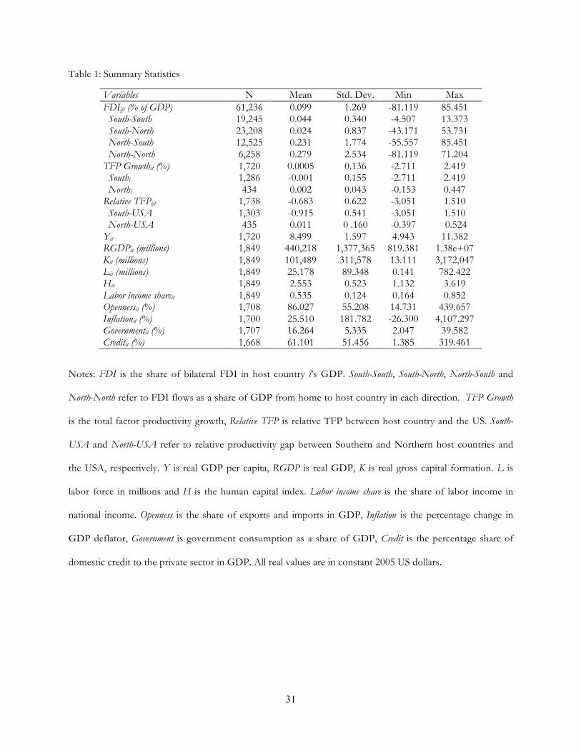
Table 1 provides summary statistics for variables used in the regression analysis. We find that the

highest level of average bilateral FDI flows are in North-North and North-South directions and are the

lowest in South-South and South-North directions. We also see that the maximums are the highest in North-

South direction, reaching as high as 85% of host country GDP, thanks to the small size of some Southern

economies. As expected, the data also reveals that average TFP growth is slower in the South than in the

North and displays a much higher variation, highlighting the greater degree of country heterogeneity among

developing countries than developed ones. The average TFP gap between the South and the productivity

frontier, the USA, is negative, highlighting the lagging TFP levels in Southern economies. We also observe

that TFP growth is significantly lower for Southern countries, which also have a bigger TFP gap with the

frontier.

<Insert Table 1 Here>

13

Figure 1 displays the share of FDI flows in host country GDPs, grouped by country-type pairs, and

suggests a significant level of country heterogeneity, particularly so within South-South and North-South

directions. One reason for this pattern is that many Southern countries have relatively smaller economies and

therefore even moderate amounts of FDI inflows measure up to significant share of their GDPs. We also

find that the North is the largest investor in both Southern and Northern host countries during the period

analyzed. The data coverage is also more complete in later years creating higher sample variation, an issue we

take up to in the sensitivity analysis section.

<Insert Figure 1 Here>

Figure 2 shows the scatter plots for TFP growth rates in the South and the North. While the TFP

growth rates of both country groups are centered around zero, there is a much higher variation within the

South than the North, again highlighting greater country heterogeneity. Figure 3 shows the Kernel densities

for the relative productivity gap between the Northern and Southern countries, and the productivity frontier,

the USA. As noted before, there is a significantly higher heterogeneity within the South than the North.

Moreover, an overwhelming majority of Southern countries lack behind the US in productivity and their

density lies to the left of the density for Northern countries, which clusters around a zero-level of

productivity gap. The density for Northern countries also confirms the OECD convergence phenomena.

<Insert Figures 2-3 Here>

4. EMPIRICAL RESULTS

Table 2 presents benchmark regression results from equation (1) using the OLS (columns 1-2), 2SLS

(columns 3-4), and the GMM methods (columns 5-6). For comparison, in columns (1), (3), and (5), we first

report results without separating host and home countries into the North and the South. We then separate

FDI flows into four directions in columns (2), (4), and (6), i.e. South-South, South-North, North-South and

North-North.12 Overall, independent of estimation method, we do not find any significant productivity

growth effect of bilateral FDI flows, either globally or in any of the four directions. None of the coefficients

are statistically or economically significant and do not yield any robust effect. The only exception is the

14

statistically (10% level) and economically marginal positive effect in South-North direction in the OLS

estimation of column (2). Yet, the coefficient loses its statistical significance and changes its sign in columns

(4) and (6) with the 2SLS and GMM estimations. The OLS results, which do not control for the endogeneity

problem, also suffer from the “attenuation bias” as the coefficient estimates are biased toward zero.

<Insert Table 2 Here>

Turning to other variables of interest, similar to previous studies and again independent of

specification or estimation method, we find that host country per capita income (Y) and financial

development (Credit) have a positive and significant effect on productivity growth. Openness to trade

(Openness) appears with a negative albeit only marginally significant economic effect. 13 Supporting the

crowding-in hypothesis, government consumption (Government) is found to have a positive but statistically

insignificant effect. Likewise, inflation appears to have a negative but statistically insignificant effect on

productivity growth. We confirm the validity of instruments used in the 2SLS and GMM analyses using the

Cragg-Donald F-statistics and the Hansen over-identification test. Despite the size of the sample, which, to

the best of our knowledge, is the largest in macro panel studies on FDI flows, the R-squared is quite high,

ranging between 0.16 and 0.22, depending on specification.

Next, in Table 3 we report regression results from Eq. (2) where we analyze the effect of FDI flows

on the productivity gap between the host country i and the frontier country j (the USA). Similar to Table 2,

we report results using the OLS (columns 1-2), 2SLS (columns 3-4) and the GMM methods (columns 5-6).

Independent of specification or the estimation method, we again do not detect any statistically or

economically significant productivity convergence effect of FDI flows globally or in any of the four directions.

In fact, all coefficient estimates for the FDI effect turn out to be negative, even though at statistically

insignificant levels, except in column (2) with the OLS estimation where South-South and North-North FDI

flows appear with a statistically marginal (10%) and economically negligible negative effect.

<Insert Table 3 Here>

15

Turning to other control variables, we find that higher per capita incomes, openness, inflation and

government consumption have a significantly positive productivity convergence effect on host countries.

Interestingly, the strongest determinants of productivity convergence are found to be the per capita incomes

and government consumption. Contrary to our expectations, the effect of financial depth appeared to be

negative, albeit with a marginal economic effect.14 Overall, Hansen over-identification test suggests that the

model is correctly specified while the Cragg-Donald F statistic rejects the null hypothesis of weak instruments.

4.1 Sensitivity analysis

To test the robustness of our findings, we conduct a variety of sensitivity tests. For space considerations, we

only report results from the 2SLS method but those from the GMM method were similar and are available in

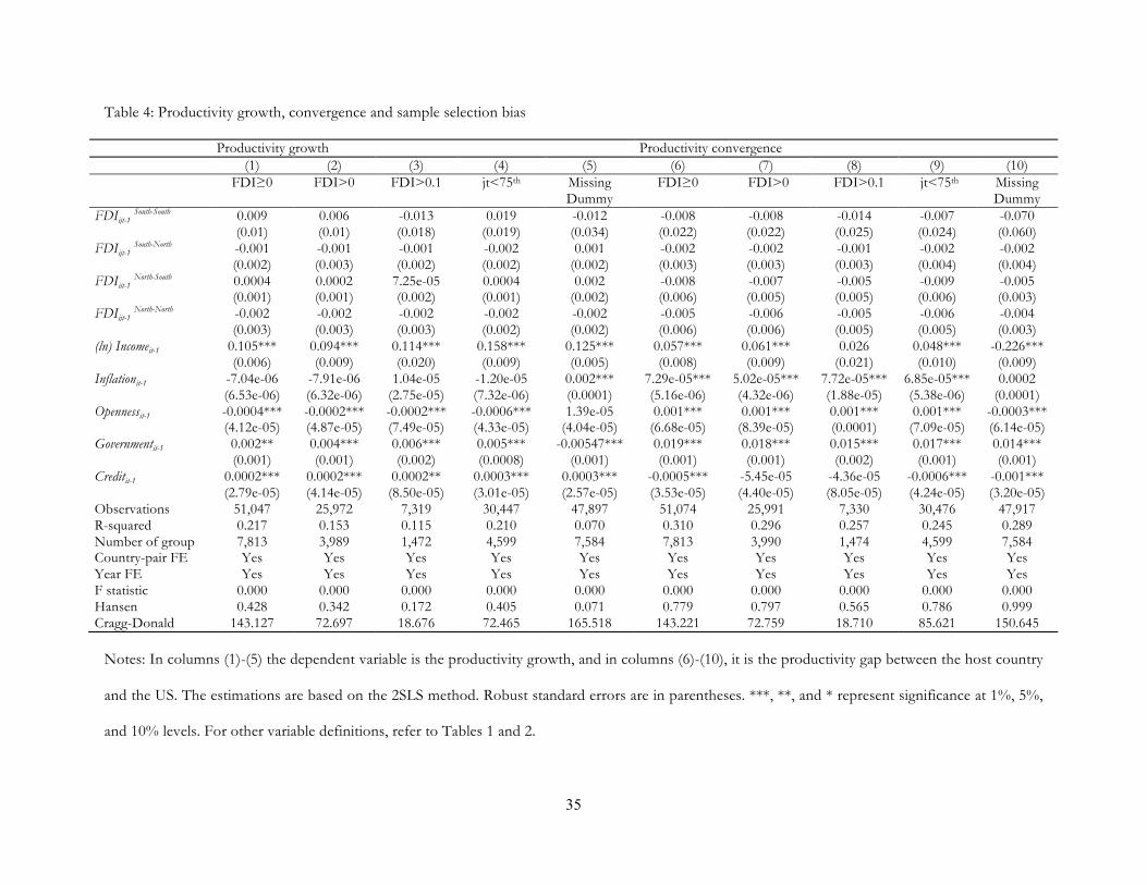
the online Appendix. We first start with the sample selection issue. As shown in Table 1, net bilateral FDI

flows (by non-residents) can be negative when outflows (including profit repatriations or exits) outweigh

inflows in a given year. In our sample, around 12% of observations are negative. While the disaggregated

nature of the data is a significant advantage in our identification strategy, one may argue that positive

productivity spillovers can only occur in the net FDI recipient countries. In addition, similar to the zero vs.

missing trade problem in the international trade literature, we have zero FDI flows between multiple country

pairs and it is impossible to know whether they are true zeros or just missing observations. Therefore,

following the Gravity literature, in Table 4 we repeat our benchmark regressions of Tables 2 and 3 after

dropping, first all negative, and then, nonpositive FDI observations. The results are presented in columns (1)-

(2) and (6)-(7) of Table 4. Next, we control for the skewed distribution of FDI flows as a significant number

of them are quite small compared to the host country economic sizes. For example, the 75th percentile of FDI

inflows (as a share of GDP) is only 0.004, which may explain why we fail to find any significant productivity

spillovers from FDI in any of the four directions. Therefore, in Columns (3) and (8), we repeat our regression

analysis by restricting the sample to those FDI inflows (as a share of GDP) that are 10% or higher.15 Third,

we test the sensitivity of our results to the duration of investments from a particular home country. In the

sample we observe a significant variation in the duration of foreign investment activity across home countries

with some having much longer investment experiences abroad. Therefore, in columns (4) and (9) we repeat

16

our benchmark regressions after dropping the top 25th percentile of the sample based on the number of home

country-year observations (i.e. 2,293).16 Fourth, the dataset we use is unbalanced and include a large number

of missing observations that may not be randomly distributed. One way to deal with this problem is to use a

censored or truncated estimation method. However, our FDI variable takes both positive and negative values

and is not censored or truncated at any specific point. To partially deal with this issue, we introduce a dummy

variable equaling one if the FDI observation is not missing, and zero otherwise. In columns (5) and (10), we

add the (unreported) lagged dummy indicators up to 10 periods to control for the occurrence pattern in case

there is some systematic reason why some countries do not receive or report FDI inflows. After these tests,

our earlier results remain unchanged.

<Insert Table 4 Here>

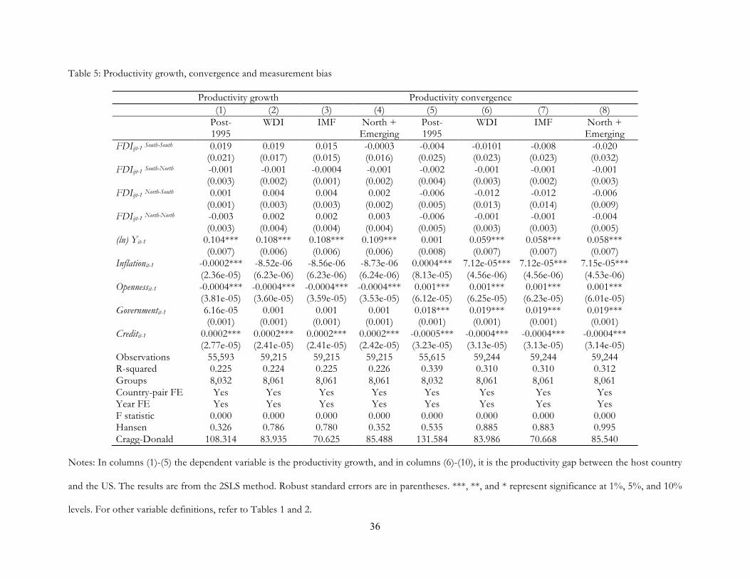
In columns (1) and (5) of Table 5 we check the sensitivity of our results to sample period given that

the data are skewed towards later years. Particularly, we repeat our regressions after limiting the sample to the

post-1995 period, which account for 90% of total observations. This is also the period that witnessed

significant changes in global economy including a radical wave of trade and financial liberalization. Next, we

consider alternative definitions of the North and the South, first for productivity growth in columns (2)-(4),

and later for productivity convergence in (6)-(8). In column (2) and (6) we redefine the North as high-income

OECD members in 2012, and then in columns (3) and (7) we adopt the International Monetary Fund (IMF)

definition of advanced economies.17 In columns (4) and (8) we experiment with including the Emerging

economies in the North rather than in the South as they may have more in common with the North than the

South (i.e. in physical and human capital, institutional infrastructure, incomes and productivity).18 Once again,

our main conclusions remain unchanged.

<Insert Table 5 Here>

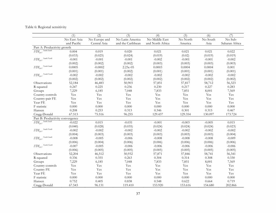
In Table 6 we test the sensitivity of our results to regional heterogeneity by dropping one

geographical region at a time from the sample (using the World Bank classification). Part A reports the results

for productivity growth and Part B reports for productivity convergence. The results are again similar to

17

those before. For space considerations, in Tables 6-9, we report results only for the FDI variables but full

results are reported in the online Appendix.

<Insert Table 6 Here>

In Table 7 we explore the sensitivity of our results from Eq. (2) to the choice of frontier country and

replace the US as the productivity frontier with the unweighted and weighted average productivity levels of

the G7 economies (using the GDP, GDP per capita and population sizes as weights).19 We again detect no

significant effect of FDI on relative productivity.

<Insert Table 7 Here>

It is possible that bilateral FDI flows are too scattered and/or too small to affect TFP growth or

convergence separately. It is also probable that flows from different home countries to the same host country

are not independent of each other and either display co-movement, or produce externalities to each other and

to the host economy collectively, which are noticeable only at the aggregate level. To test these possibilities,

we aggregate bilateral flows at the host country level in columns (1) and (5) of Table 8 so that FDI flows

capture total FDI flows in each direction. In columns (2) and (6), we look at the effect of aggregate FDI flows

without separating their direction. In columns (3)-(4) and (7)-(8), we repeat the same exercise by focusing on

Southern and Northern host countries alone to test the productivity effects of aggregate FDI flows. After

these exercises, we still do not find any robust or economically and statistically significant productivity growth

or convergence effect from FDI flows. While in Column (1), we find a positive effect from South-South and

South-North flows and a negative effect from North-North flows, these are statistically and economically

marginal effects and are not robust to estimation method.20 As for Column (5), the positive convergence

effect from South-North flows (at 5% significance level) drop by half in size and significance level (to 10%) in

the GMM estimation (which is reported in the online Appendix).

<Insert Table 8 Here>

18

Another possible source of estimation error is that missing observations in the sample reflect some

systematic reporting error between certain country pairs. To control for this possibility, we created a strongly

balanced panel for all possible country pairs and then used the Heckman two-step procedure to control for

the selection bias in the first stage. We experimented with different methods to choose the threshold level of

truncation including the following: i) We first took the absolute values of FDI variable to make all the

observations non-negative and introduced a dummy variable for positive FDI flows (equaling one if FDI is

positive, and zero otherwise). ii) Second, we repeated the same exercise but treated zero FDI flows as missing.

iii) Third, we kept only non-negative FDI flows, including zero flows. iv) Fourth, we kept only positive FDI

flows and treated zero and missing observations both as missing. We then run the Heckman two-step

procedure so that in the selection equation we run a probit model and estimated the inverse mills ratio to be

included in the second equation to control for the selection bias. After these exercises, all our earlier results

remain unchanged as we do not detect any significant productivity growth or convergence effect of FDI

flows even after controlling for the selection bias. We report the regression results in the online Appendix.

One issue that we have not yet controlled for is the possible non-linearity in FDI effects. To test for

this possibility, we included the squared term of FDI and repeated our earlier regression analysis for

productivity growth and convergence effects. As reported in the online Appendix, we do not detect any

nonlinear effects of FDI flows as the squared term is found to be insignificant.

As argued by Borensztein et al. (1998), Xu (2000) and Damijan et al. (2013), the productivity effects

of FDI flows may be conditional on host countries’ absorptive capabilities. To test for this possibility, we

introduce two interaction terms for human capital (HK), as measured by human capital per person index

from PWT 8.1, and economic openness, measured by the share of exports and imports in GDP. As reported

in Table 9, our results remain mostly unchanged as the interaction terms came out insignificant, so did the net

effect of FDI flows. However, we find that the level of human capital has a significantly positive effect on

both TFP growth and TFP convergence. Furthermore, we show that human capital interaction with FDI is

positive and significant in South-South direction for TFP convergence, and yet it is not strong enough to turn

the net effect of FDI into a positive and significant magnitude.

19

<Insert Table 9 Here>

4.2 A decomposition analysis: TFP vs. physical and human capital growth

While we have not found any significant or robust productivity growth or convergence effect from FDI, a

growth decomposition exercise can allow us to examine whether other components of aggregate growth in

Eq. (3) respond differently to FDI. Particularly, we replace the dependent variable in Eq. (1) with the physical

capital growth (columns (1)-(4)) and human capital growth (columns (5)-8)) and report the results from the

2SLS and GMM estimations in Table 9. To make comparison easier with previous studies, we also include the

aggregated FDI flows variable in columns (1)-(2) and (5)-(6). Similar to Alfaro et al. (2009) and independent

of the estimation method in columns (1)-(4), we do not find any significant effect of aggregate or bilateral

FDI flows on physical capital growth. Turning to columns (5)-(6), however, we detect a significantly positive

effect of aggregate FDI flows on human capital growth. Furthermore, when we focus on bilateral flows, we

find that the positive effect is present in only one direction that is South-South.

<Insert Table 10 Here>

4.3 Sector-specific productivity effects

The sectoral composition of FDI, as discussed earlier, can be a significant determinant of productivity effects.

Manufacturing FDI, for example, can have different effects both on intra and inter-industry productivity

growth than services or agricultural FDI. Likewise, sectoral distribution of FDI is likely to be time-variant and

heterogeneous across different home and host countries. In our regression analysis we used aggregate bilateral

FDI flows given that there is no bilateral FDI data for most of our sample countries at the sectoral level.

Regarding sectoral TFP, while sectoral output and employment data are available, sectoral capital stock data

are quite sketchy and are available only for few countries, mostly from the OECD. Human capital variable is

even more problematic as it is not available at the sectoral level. Another issue is the lack of income shares

data at the sectoral level. These problems make the calculation of sectoral TFP quite difficult. Having said this,

however, we experimented with two sector-specific productivity variables: i) Labor productivity, measured by

sectoral valued added/sectoral employment for 165 countries, and ii) Sectoral TFP for 39 countries. Both

20

variables are calculated for the agricultural, services, and industry sectors and the details of variable definitions

are provided in the online Appendix. Because of data unavailability, sectoral TFP calculations assumed that

the human capital and income shares are the same across sectors. Using these two proxies of sectoral

productivity, we repeated our empirical analysis of Tables 2 and 3 for TFP growth and convergence effects.

Given the space limitations, we reported results from these exercises in the online Appendix. Confirming our

previous findings, we continue to find an insignificant TFP growth or convergence effect from bilateral FDI

flows even at the sectoral level.21

5. CONCLUSION

In spite of a significant increase in global investment flows, there is no conclusive evidence showing that FDI

stimulates productivity or aggregate growth in host countries. In this paper we contribute to this debate by

addressing two issues that were previously unexplored, which are the aggregation bias in FDI flows and the

home and host country heterogeneity. Instead of relying on aggregate FDI flows, which are highly

heterogeneous by nature, we built a unique dataset on bilateral FDI flows between 240 host and 243 home

countries between 1990 and 2012. Using bilateral flows, we were then able to control for investor and country

heterogeneity including home and host country characteristics as well as any differences in the time series

properties of the data. Furthermore, we also accounted for unobserved country heterogeneity within and

between different groups based on economic development levels. The empirical results using a variety of

estimation techniques and a rich battery of sensitivity checks suggest that bilateral FDI flows do not have a

significant or robust productivity growth enhancing effect in host countries. Likewise, we do not detect any

productivity convergence effect between host countries and the productivity frontier(s). We also find no

evidence of any productivity spillover difference between FDI flows in any of the four directions that are

South-South, South-North, North-South or North-North. Our results remained unchanged when we

accounted for the absorptive capabilities of host countries, measured by human capital and trade openness. In

a decomposition exercise we also fail to find any significant effect of FDI flows in any four directions on

physical capital growth. However, we find some evidence showing a significantly positive effect of FDI flows

on human capital growth but only in one direction, the South-South. Last but not least, when examining

21

sectoral productivity effects, we find no significant effect of bilateral aggregate FDI flows on agricultural,

services or industry productivity growth or convergence.

We should note, however, that our findings do not settle the debate on the productivity effects of

FDI once and for all. While we tackle the direction of flows as well as country heterogeneity, there are other

issues that our study does not address. Particularly, we hope that future studies will be able to shed further

light on the sectoral heterogeneity of FDI flows while at the same time accounting for country and investor

heterogeneity. Particularly, while there is evidence showing productivity convergence within manufacturing

industries across countries, the same is not true for any other sector (Rodrik, 2013). As a result, we are more

likely to find productivity enhancing effects of FDI flows when they are in manufacturing industries. There is

also a need to explore further the inter-sectoral spillover effects from FDI, as is attempted in Fernandes and

Paunov (2012). Furthermore, there is a need to differentiate merger and acquisitions from greenfield FDI as

they may have different productivity-inducing effects.

Finally, a word of caution for policy makers might be in place here. Ours as well as previous studies’

findings highlight the importance of FDI heterogeneity, which might be a determining factor for FDI

effectiveness. If this is indeed the case, one size fits all type government policies to attract FDI may be

ineffective. Instead, governments and policy makers should concentrate their efforts to identify what types of

FDI flows are productivity enhancing and then develop their policies accordingly. Obviously, such an

undertaking will require an active industrial policy to enhance the effectiveness of foreign investment and to

widen the scope and scale of linkages between domestic and foreign investments.

22

REFERENCES

Aghion, P., Bacchetta, P., Ranciere, R., & Rogoff, K. (2009). Exchange rate volatility and productivity

growth: The role of financial development. Journal of Monetary Economics, 56(4), 494-513.

Agyei-Holmes, A. (2016). Tilling the soil in Tanzania: What do Emerging economies have to offer? The

European Journal of Development Research 28 (3), 379-396.

Aitken, Brian J., and Ann E. Harrison (1999), Do domestic firms benefit from direct foreign investment?

Evidence from Venezuela. American Economic Review, 89, 605-618.

Aleksynska, M., and Havrylchyk, O. (2013). FDI from the South: the role of institutional distance and

natural resources. European Journal of Political Economy, 29, 38-53.

Alfaro, L., Kalemli‐Ozcan, S., and Sayek, S. (2009). FDI, productivity and financial development. The

World Economy, 32(1), 111-135.

Amighini, A., and Sanfilippo, M. (2014). Impact of South–South FDI and trade on the export upgrading

of African economies. World Development, 64, 1-17.

Amsden, A. (1987). The directionality of trade: Historical perspective and overview. In O. Havrylyshin

(ed.), World Bank Symposium: Exports of Developing Countries: How Direction Affects Performance, 123–

38. Washington, DC: World Bank.

Amsden, A. (1980). The industry characteristics of intra-Third World trade in manufactures. Economic

Development and Cultural Change 29(1), 1–19.

Arnold, J. and Javorcik, B. (2009), Gifted kids or pushy parents? Foreign direct investment and plant

productivity in Indonesia. Journal of International Economics, 79(1), 42-53.

Atta-Ankomah, R. (2014). China’s Presence in Developing Countries’ Technology Basket: The Case of

Furniture Manufacturing in Kenya. PhD thesis The Open University, UK.

Bahar, D., Hausmann, R., and Hidalgo, C. A. (2014). Neighbors and the evolution of the comparative

advantage of nations: Evidence of international knowledge diffusion? Journal of International Economics, 92(1),

111-123.

23

Bartelsman, E.J. and Doms, M. (2000) Understanding productivity: Lessons from longitudinal microdata.

Journal of Economic Literature, 38(3), 569-594.

Bitros, G. C., and Panas, E. E. (2006). The inflation-productivity trade-off revisited. Journal of Productivity

Analysis 26(1), 51-65.

Borensztein, E., De Gregorio, J. and Lee, J.W. (1998). How Does Foreign Direct Investment Affect

Economic Growth? Journal of International Economics 45, 115-135.

Bwalya, S. M. (2006). Foreign direct investment and technology spillovers: Evidence from panel data

analysis of manufacturing firms in Zambia. Journal of Development Economics, 81(2), 514-526.

Cameron, G., Proudman, J., and Redding, S. (2005). Technological convergence, R&D, trade and

productivity growth. European Economic Review, 49(3), 775-807.

Dahi, O.S. and Demir, F. (2016). South-South Trade and Finance in the 21st Century: Rise of the South or a Second

Great Divergence. Anthem Press: New York.

Damijan, J.P., Rojec, M., Majcen, B. and Knell, M. (2013) Impact of Firm Heterogeneity on Direct and

Spillover Effects of FDI: Micro Evidence from Ten Transition Countries. Journal of Comparative Economics 41,

895-922.

De Mello, L. R. (1999). Foreign direct investment-led growth: evidence from time series and panel data.

Oxford Economic Papers, 51(1), 133-151.

Demir, F. and Hu, C. (2016). Institutional differences and direction of bilateral FDI flows: Are South-

South Flows any different than the rest? World Economy 39(12): 2000 – 2024.

Demir, F. and Su, L. (2016). Total factor productivity, foreign direct investment and entry barriers in

Chinese automobile industry. Emerging Markets Finance and Trade 52(2): 302 – 321.

Djankov, S. and Hoekman, B. (2000), Foreign Investment and Productivity Growth in Czech

Enterprises. The World Bank Economic Review, 14(1), 49-64.

Doytch, N., and Uctum, M. (2011). Does the worldwide shift of FDI from manufacturing to services

accelerate economic growth? A GMM estimation study. Journal of International Money and Finance 30(3), 410-427.

24

Fernandes, A. and Paunov, C. (2012). Foreign direct investment in services and manufacturing

productivity: Evidence for Chile. Journal of Development Economics, 97(2), 305–321.

Fons-Rosen, C., Kalemli-Ozcan, S., Sorensen, B.E., Villegas-Sanchez, C., Volosovych, V., 2014. Foreign

Ownership, Selection, and Productivity. CompNet, Working Paper, March.

Fu, X. (2008). Foreign direct investment, absorptive capacity and regional innovation capabilities:

Evidence from China. Oxford Development Studies, 36(1), 89-110.

Fu, X., and Gong, Y. (2011). Indigenous and foreign innovation efforts and drivers of technological

upgrading: Evidence from China. World Development, 39(7), 1213-1225.

Girma, S., Gong, Y., Görg, H., and Lancheros, S. (2015). Estimating direct and indirect effects of

foreign direct investment on firm productivity in the presence of interactions between firms. Journal of

International Economics, 95(1), 157-169.

Go ̈rg, Holger, and Strobl, E. (2001). Multinational companies and productivity spillovers: A meta-

analysis. Economic Journal 111(475), 723-739.

Griffith, R., Redding, S., and Van Reenen, J. (2004). Mapping the two faces of R&D: productivity

growth in a panel of OECD industries. Review of Economics and Statistics 86(4), 883-895.

Haddad, M., and Harrison, A. (1993). Are there positive spillovers from direct foreign investment?:

Evidence from panel data for Morocco. Journal of Development Economics, 42(1), 51-74.

Harris, R., and Moffat, J. (2013). The Direct Contribution of FDI to Productivity Growth in Britain,

1997–2008. The World Economy, 36(6), 713-736.

Harris, R.I.D., and Robinson, C. (2002). The impact of foreign acquisitions on total factor productivity:

Plant-level evidence from UK manufacturing 1987- 1992. Review of Economics and Statistics, 84, 562-568

Haskel, J., Pereira, S., and Slaughter, M. (2007). Does inward foreign direct investment boost the

productivity of domestic firms? Review of Economics and Statistics, 89(3), 482-496.

Hulten, C. R. (2001). Total factor productivity: a short biography. In C.R. Hulten, E. R. Dean and M.J.

Harper (Eds.), New Developments in Productivity Analysis (pp. 1-54). University of Chicago Press.

25

Kaplinsky R. (1990). The Economies of Small: Appropriate Technology in a Changing World, London:

Intermediate Technology Publications.

Kaplinsky, R. (2013). What Contribution Can China Make To Inclusive Growth In SSA? Development and

Change, 44(6), 1295-1316.

Keller, W., and Yeaple, S. R. (2003). Multinational enterprises, international trade, and productivity growth: firm-

level evidence from the United States (No. w9504). National Bureau of Economic Research.

Kokko, A., Tansini, R., and Zejan, M. C. (1996). Local technological capability and productivity

spillovers from FDI in the Uruguayan manufacturing sector. The Journal of Development Studies 32(4), 602-611.

Lall, S. (2000). The technological structure and performance of developing country manufactured

exports, 1985–1998. Oxford Development Studies 28(3), 337–70.

Lee, J. (2009). Trade, FDI, and productivity convergence: A dynamic panel data approach in 25

countries. Japan and the World Economy, 21(3), 226-238.

Levine, R., Loayza, N., Beck, T. (2000). Financial intermediation and growth: causality and causes. Journal

of Monetary Economics 46, 31--77.

Liu, Z. (2008). Foreign direct investment and technology spillovers: Theory and evidence. Journal of

Development Economics 85(1-2), 176-193.

Mayer‐Foulkes, D., and Nunnenkamp, P. (2009). Do multinational enterprises contribute to

convergence or divergence? A disaggregated analysis of US FDI. Review of Development Economics 13(2), 304-318.

Miller, S. M., and Upadhyay, M. P. (2000). The effects of openness, trade orientation, and human capital

on total factor productivity. Journal of Development Economics 63(2), 399-423.

National Science Foundation (NSF) (2014) Science and Engineering Indicators 2014, NSF. Downloaded

from http://www.nsf.gov/statistics/seind14/index.cfm/appendix/tables.htm#c4 Accessed on 12/8/2015.

Nelson, R. and Pack, H. (1999). The Asian miracle and modern growth theory. Economic Journal, 109(457),

416–36.

Peden, E. A., and Bradley, M. D. (1989). Government size, productivity, and economic growth: The

post-war experience. Public Choice, 61(3), 229-245.

26

Rodrik, D. (2013). Unconditional convergence in manufacturing. The Quarterly Journal of Economics 128(1),

165–204.

Schaffer, M.E. (2010). xtivreg2: Stata module to perform extended IV/2SLS, GMM and AC/HAC,

LIML and k-class regression for panel data models. http://ideas.repec.org/c/boc/bocode/s456501.html

Schiff, M. and Wang, Y. and Ollareaga, M. 2002. Trade-related technology diffusion and the dynamics

of North-South and South-South integration. World Bank Policy Research WP No. 2861.

Schiff, M., and Wang, Y. (2008). North-south and south-south trade-related technology diffusion: How

important are they in improving tfp growth?. The Journal of Development Studies 44(1), 49-59.

Stewart, F. (1982). Technology and Underdevelopment, 2nd edition, London: Macmillan.

Stewart, F. (1992). North-South and South-South: Essays on International Economics. Hong Kong: St. Martin’s

Press.

Stewart, F. (1992). North-South and South-South: Essays on International Economics. Hong Kong: St. Martin’s

Press.

Stock J., and Yogo, M. (2005) Testing for Weak Instruments in Linear IV Regression. In Andrews DWK

(Ed.) Identification and Inference for Econometric Models. New York: Cambridge University Press, pp. 80-

108.

UNCTAD (2011). World Investment Report 2011. New York and Geneva: United Nations.

UNCTAD (2014) World Investment Report 2014. New York and Geneva: United Nations.

UNCTAD (2016). UNCTAD Online FDI Database. UNCTADSTAT. Accessed on 4/1/2016.

Xu, B. (2000) Multinational Enterprises, Technology Diffusion, and Host Country Productivity Growth.

Journal of Development Economics 62, 477-493.

Xu, H., Wan, D., Sun, Y. (2014). Technology Spillovers of Foreign Direct Investment in Coastal Regions

of East China: A Perspective on Technology Absorptive Capacity. Emerging Markets Finance and Trade 50(1S),

96-106.

27

Xu, X., Li, X., Qi, G., Tang, L., Mukwereza, L. (2016). Science, Technology, and the Politics of

Knowledge: The Case of China’s Agricultural Technology Demonstration Centers in Africa. World Development

81, 82-91.

Yasar, M. and Paul, C. (2009). Size and Foreign Ownership Effects on Productivity and Efficiency: An

Analysis of Turkish Motor Vehicle and Parts Plants. Review of Development Economics, 13(4), 576-591.

28

ENDNOTES

1The South includes all non-high-income OECD countries as well as South Korea and Hong Kong.

2The choice of estimation methodology is reported to have an effect on the results. For a discussion see

Go ̈rg and Strobl (2001) and Girma et al. (2015).

3 We find no evidence of spurious regressions caused by any correlation between the four FDI variables and

other controls as the cross correlation between them is found to be in the range of [-0.006, 0.065]. We included

the full correlation matrix in the online Appendix.

4 Stock and Yogo (2005) provide the critical values for this F-test.

5 The 2SLS and GMM estimates are obtained using the xtivreg2 command in Stata 13.0 by Schaffer (2010).

6 We should note that TFP also includes measurement error and omitted variables, and therefore can be

interpreted simply as a measure of our ignorance.

7 Some simplifying assumptions are needed here. First, technology advancement is Hicks-neutral and can be

separated from the input variables. Second, the inputs market is competitive and each input is paid its

marginal product so that we can use their income shares instead of output elasticities.

8 We also experimented with the conventional assumption and made α equal to 1/3 and β to 2/3. The

(unreported) results were highly similar and are available in the online appendix.

9 Törnqvist index uses the average value shares in the consecutive periods as weights, and helps smooth out

the volatility in income shares.

10 The data from these three sources are merged using the following procedure. For FDI inflows and

outflows to and from OECD members, we used the OECD dataset. For FDI flows from and to non-OECD

members, we used the UNCTAD and/or individual country data. When there is discrepancy between inflows

to i and outflows from j, we used the host country data for those that are both (or none) high-income OECD

members. If only one of the countries is high-income OECD, we gave priority to its inflows and outflows

data over others. The data in non-USD currencies are converted to the USD using average annual exchange

rates from the IMF.

29

11 The results are robust to the use of alternative GDP and capital stock series in current or constant

international dollars from the PWT. However, the use of the PWT data reduces the sample size considerably.

12 In the online Appendix, we report a bare-bones version of Table 2, dropping all controls except the real

GDP per capita.

13 The results remain practically unchanged when we exclude Openness from the regressions.

14 Excluding this variable does not affect any of our results. It is also possible that financial development is

negatively correlated with productivity in the short run due to financial fragility during the transitionary

period (Loayza and Ranciere, 2006).

15 We also used alternative thresholds such as 5%, 15% and 20%, and also removed the top and bottom 1%.

Additionally, we dropped the top and bottom one percentiles using GDP per capita. The results were similar.

16 We test different thresholds by limiting the sample to those above the 25th as well as the 75th percentiles.

17 High-income OECD countries include: Australia, Austria, Belgium, Canada, Chile, Czech Republic,

Denmark, Estonia, Finland, France, Germany, Greece, Hungary, Iceland, Ireland, Italy, Israel, Japan,

Luxembourg, Netherlands, New Zealand, Norway, Poland, Portugal, Slovak Republic, Slovenia, South Korea,

Spain, Sweden, Switzerland, U.K., and U.S. The IMF definition of Advanced economies includes: Australia,

Austria, Belgium, Canada, Cyprus, Czech Republic, Denmark, Estonia, Finland, France, Germany, Greece,

Hong Kong, Iceland, Ireland, Italy, Israel, Japan, Latvia, Lithuania, Luxembourg, Malta, Netherlands, New

Zealand, Norway, Portugal, San Marino, Singapore, Slovakia, Slovenia, South Korea, Spain, Sweden,

Switzerland, Taiwan, U.K. and U.S.

18 We follow the IMF, FTSE, Standard & Poor’s, and Dow Jones to define the Emerging economies,

including: Argentina, Brazil, Chile, China, Colombia, Czech Republic, Estonia, Egypt, Hungary, India,

Indonesia, Malaysia, Mexico, Morocco, Nigeria, Pakistan, Peru, Philippines, Poland, Romania, Russia,

Slovakia, Slovenia, South Africa, South Korea, Thailand and Turkey.

19 The G7 includes Canada, France, Germany, Italy, Japan, U.K and U.S.

20 As reported in the online Appendix Table 8b, except for the South-South FDI flows (at 10% level), other

FDI variables in the growth equation become insignificant in the GMM estimation.

30

21 While bilateral sectoral FDI data are not available, if sectoral distribution of FDI is homogenous within

each group of countries, our identification will control any sectoral composition differences in FDI flows.

31

Table 1: Summary Statistics

Variables N Mean Std. Dev. Min Max FDIijt (% of GDP) 61,236 0.099 1.269 -81.119 85.451 South-South 19,245 0.044 0.340 -4.507 13.373 South-North 23,208 0.024 0.837 -43.171 53.731 North-South 12,525 0.231 1.774 -55.557 85.451 North-North 6,258 0.279 2.534 -81.119 71.204 TFP Growthit (%) 1,720 0.0005 0.136 -2.711 2.419 Southi 1,286 -0.001 0.155 -2.711 2.419 Northi 434 0.002 0.043 -0.153 0.447 Relative TFPijt 1,738 -0.683 0.622 -3.051 1.510 South-USA 1,303 -0.915 0.541 -3.051 1.510 North-USA 435 0.011 0 .160 -0.397 0.524 Yit 1,720 8.499 1.597 4.943 11.382 RGDPit (millions) 1,849 440,218 1,377,365 819.381 1.38e+07 Kit (millions) 1,849 101,489 311,578 13.111 3,172,047 Lit (millions) 1,849 25.178 89.348 0.141 782.422 Hit 1,849 2.553 0.523 1.132 3.619 Labor income shareit 1,849 0.535 0.124 0.164 0.852 Opennessit (%) 1,708 86.027 55.208 14.731 439.657 Inflationit (%) 1,700 25.510 181.782 -26.300 4,107.297 Governmentit (%) 1,707 16.264 5.335 2.047 39.582 Creditit (%) 1,668 61.101 51.456 1.385 319.461

Notes: FDI is the share of bilateral FDI in host country i’s GDP. South-South, South-North, North-South and

North-North refer to FDI flows as a share of GDP from home to host country in each direction. TFP Growth

is the total factor productivity growth, Relative TFP is relative TFP between host country and the US. South-

USA and North-USA refer to relative productivity gap between Southern and Northern host countries and

the USA, respectively. Y is real GDP per capita, RGDP is real GDP, K is real gross capital formation. L is

labor force in millions and H is the human capital index. Labor income share is the share of labor income in

national income. Openness is the share of exports and imports in GDP, Inflation is the percentage change in

GDP deflator, Government is government consumption as a share of GDP, Credit is the percentage share of

domestic credit to the private sector in GDP. All real values are in constant 2005 US dollars.

32

Table 2: Productivity growth and FDI flows: North vs. South

(1) (2) (3) (4) (5) (6) OLS OLS 2SLS 2SLS GMM GMM FDIijt-1 0.0001 0.004 0.004 (0.0002) (0.003) (0.003) FDIijt-1 South-South 0.004 0.021 0.022 (0.003) (0.019) (0.019) FDIijt-1 South-North 0.0003* -0.001 -0.001 (0.0001) (0.003) (0.003) FDIijt-1 North-South 1.87e-05 0.0004 0.0003 (0.0004) (0.001) (0.001) FDIijt-1 North-North 0.0001 -0.002 -0.002 (0.0002) (0.002) (0.002) (ln)Yit-1 0.153*** 0.153*** 0.109*** 0.108*** 0.109*** 0.108*** (0.011) (0.011) (0.006) (0.006) (0.006) (0.006) Inflationit-1 -9.36e-06*** -9.33e-06*** -8.68e-06 -8.63e-06 -8.70e-06 -8.70e-06 (2.93e-06) (2.92e-06) (6.24e-06) (6.23e-06) (6.24e-06) (6.23e-06) Opennessit-1 -0.0004*** -0.0004*** -0.0004*** -0.0004*** -0.0004*** -0.0004*** (3.91e-05) (3.91e-05) (3.56e-05) (3.56e-05) (3.56e-05) (3.55e-05) Governmentit-1 0.008*** 0.008*** 0.001 0.001 0.001 0.001 (0.0008) (0.0008) (0.001) (0.001) (0.001) (0.001) Creditit-1 -0.0001*** -0.0001*** 0.0002*** 0.0002*** 0.0002*** 0.0002*** (2.96e-05) (2.96e-05) (2.42e-05) (2.41e-05) (2.42e-05) (2.41e-05) Observations 83,518 83,518 59,215 59,215 59,215 59,215 R-squared 0.162 0.162 0.224 0.225 0.224 0.225 Groups 10,305 10,305 8,061 8,061 8,061 8,061 Country-pair FE Yes Yes Yes Yes Yes Yes Year FE Yes Yes Yes Yes Yes Yes F-statistic 0.000 0.000 0.000 0.000 0.000 0.000 Hansen - - 0.412 0.310 0.412 0.310 Cragg-Donald - - 413.139 132.456 413.139 132.456

33

Notes: Dependent variable is the host country TFP growth. Robust standard errors are in parentheses, ***, **, and * represent significance at 1%, 5%,

and 10% levels. Groups refer to the number of country pairs. Year FE is year fixed effects. Test statistics, except for Cragg-Donald F-statistics are given

by their p-values. Hansen is the Hansen overidentification test. For other variable definitions, refer to Table 1.

34

Table 3: Productivity convergence and FDI flows: North vs. South

(1) (2) (3) (4) (5) (6) OLS OLS 2SLS 2SLS GMM GMM FDIijt-1 -0.0004 -0.005 -0.004 (0.0006) (0.004) (0.004) FDIijt-1

South-South -0.009* -0.004 -0.002 (0.005) (0.024) (0.024) FDIijt-1

South-North 0.0004 -0.002 -0.002 (0.0006) (0.003) (0.003) FDIijt-1

North-South -0.0002 -0.008 -0.008 (0.002) (0.006) (0.006) FDIijt-1

North-North -0.0005* -0.006 -0.006 (0.0003) (0.005) (0.005) (ln)Yit-1 0.027** 0.027** 0.057*** 0.057*** 0.057*** 0.056*** (0.014) (0.014) (0.007) (0.007) (0.007) (0.007) Inflationit-1 5.97e-05*** 5.96e-05*** 7.15e-05*** 7.14e-05*** 7.15e-05*** 7.15e-05*** (6.61e-06) (6.61e-06) (4.53e-06) (4.54e-06) (4.53e-06) (4.54e-06) Opennessit-1 0.002*** 0.002*** 0.001*** 0.001*** 0.001*** 0.001*** (8.01e-05) (8.02e-05) (5.88e-05) (5.96e-05) (5.87e-05) (5.95e-05) Governmentit-1 0.013*** 0.013*** 0.019*** 0.019*** 0.019*** 0.019*** (0.001) (0.001) (0.001) (0.001) (0.001) (0.001) Creditit-1 -0.0004*** -0.0004*** -0.0004*** -0.0004*** -0.0004*** -0.0004*** (5.46e-05) (5.46e-05) (3.13e-05) (3.14e-05) (3.13e-05) (3.14e-05) Observations 83,721 83,721 59,244 59,244 59,244 59,244 R-squared 0.246 0.246 0.312 0.309 0.312 0.309 Groups 10,441 10,441 8,061 8,061 8,061 8,061 Country-pair FE Yes Yes Yes Yes Yes Yes Year FE Yes Yes Yes Yes Yes Yes F statistic 0.000 0.000 0.000 0.000 0.000 0.000 Hansen - - 0.683 0.639 0.683 0.639 Cragg-Donald - - 415.053 157.296 415.053 157.296

Notes: Dependent variable is the productivity gap between a host country and the US. Robust standard errors are in parentheses. ***, **, and *

represent significance at 1%, 5%, and 10% levels. For variable definitions, refer to Tables 1 and 2.

35

Table 4: Productivity growth, convergence and sample selection bias

Productivity growth Productivity convergence (1) (2) (3) (4) (5) (6) (7) (8) (9) (10) FDI≥0 FDI>0 FDI>0.1 jt<75th Missing

Dummy FDI≥0 FDI>0 FDI>0.1 jt<75th Missing

Dummy FDIijt-1

South-South 0.009 0.006 -0.013 0.019 -0.012 -0.008 -0.008 -0.014 -0.007 -0.070 (0.01) (0.01) (0.018) (0.019) (0.034) (0.022) (0.022) (0.025) (0.024) (0.060) FDIijt-1

South-North -0.001 -0.001 -0.001 -0.002 0.001 -0.002 -0.002 -0.001 -0.002 -0.002 (0.002) (0.003) (0.002) (0.002) (0.002) (0.003) (0.003) (0.003) (0.004) (0.004) FDIijt-1

North-South 0.0004 0.0002 7.25e-05 0.0004 0.002 -0.008 -0.007 -0.005 -0.009 -0.005 (0.001) (0.001) (0.002) (0.001) (0.002) (0.006) (0.005) (0.005) (0.006) (0.003) FDIijt-1

North-North -0.002 -0.002 -0.002 -0.002 -0.002 -0.005 -0.006 -0.005 -0.006 -0.004 (0.003) (0.003) (0.003) (0.002) (0.002) (0.006) (0.006) (0.005) (0.005) (0.003) (ln) Incomeit-1 0.105*** 0.094*** 0.114*** 0.158*** 0.125*** 0.057*** 0.061*** 0.026 0.048*** -0.226*** (0.006) (0.009) (0.020) (0.009) (0.005) (0.008) (0.009) (0.021) (0.010) (0.009) Inflationit-1 -7.04e-06 -7.91e-06 1.04e-05 -1.20e-05 0.002*** 7.29e-05*** 5.02e-05*** 7.72e-05*** 6.85e-05*** 0.0002 (6.53e-06) (6.32e-06) (2.75e-05) (7.32e-06) (0.0001) (5.16e-06) (4.32e-06) (1.88e-05) (5.38e-06) (0.0001) Opennessit-1 -0.0004*** -0.0002*** -0.0002*** -0.0006*** 1.39e-05 0.001*** 0.001*** 0.001*** 0.001*** -0.0003*** (4.12e-05) (4.87e-05) (7.49e-05) (4.33e-05) (4.04e-05) (6.68e-05) (8.39e-05) (0.0001) (7.09e-05) (6.14e-05) Governmentit-1 0.002** 0.004*** 0.006*** 0.005*** -0.00547*** 0.019*** 0.018*** 0.015*** 0.017*** 0.014*** (0.001) (0.001) (0.002) (0.0008) (0.001) (0.001) (0.001) (0.002) (0.001) (0.001) Creditit-1 0.0002*** 0.0002*** 0.0002** 0.0003*** 0.0003*** -0.0005*** -5.45e-05 -4.36e-05 -0.0006*** -0.001*** (2.79e-05) (4.14e-05) (8.50e-05) (3.01e-05) (2.57e-05) (3.53e-05) (4.40e-05) (8.05e-05) (4.24e-05) (3.20e-05) Observations 51,047 25,972 7,319 30,447 47,897 51,074 25,991 7,330 30,476 47,917 R-squared 0.217 0.153 0.115 0.210 0.070 0.310 0.296 0.257 0.245 0.289 Number of group 7,813 3,989 1,472 4,599 7,584 7,813 3,990 1,474 4,599 7,584 Country-pair FE Yes Yes Yes Yes Yes Yes Yes Yes Yes Yes Year FE Yes Yes Yes Yes Yes Yes Yes Yes Yes Yes F statistic 0.000 0.000 0.000 0.000 0.000 0.000 0.000 0.000 0.000 0.000 Hansen 0.428 0.342 0.172 0.405 0.071 0.779 0.797 0.565 0.786 0.999 Cragg-Donald 143.127 72.697 18.676 72.465 165.518 143.221 72.759 18.710 85.621 150.645

Notes: In columns (1)-(5) the dependent variable is the productivity growth, and in columns (6)-(10), it is the productivity gap between the host country

and the US. The estimations are based on the 2SLS method. Robust standard errors are in parentheses. ***, **, and * represent significance at 1%, 5%,

and 10% levels. For other variable definitions, refer to Tables 1 and 2.

36

Table 5: Productivity growth, convergence and measurement bias

Productivity growth Productivity convergence (1) (2) (3) (4) (5) (6) (7) (8) Post-

1995 WDI IMF North +

Emerging Post- 1995

WDI IMF North + Emerging

FDIijt-1 South-South 0.019 0.019 0.015 -0.0003 -0.004 -0.0101 -0.008 -0.020 (0.021) (0.017) (0.015) (0.016) (0.025) (0.023) (0.023) (0.032) FDIijt-1 South-North -0.001 -0.001 -0.0004 -0.001 -0.002 -0.001 -0.001 -0.001 (0.003) (0.002) (0.001) (0.002) (0.004) (0.003) (0.002) (0.003) FDIijt-1 North-South 0.001 0.004 0.004 0.002 -0.006 -0.012 -0.012 -0.006 (0.001) (0.003) (0.003) (0.002) (0.005) (0.013) (0.014) (0.009) FDIijt-1 North-North -0.003 0.002 0.002 0.003 -0.006 -0.001 -0.001 -0.004 (0.003) (0.004) (0.004) (0.004) (0.005) (0.003) (0.003) (0.005) (ln) Yit-1 0.104*** 0.108*** 0.108*** 0.109*** 0.001 0.059*** 0.058*** 0.058*** (0.007) (0.006) (0.006) (0.006) (0.008) (0.007) (0.007) (0.007) Inflationit-1 -0.0002*** -8.52e-06 -8.56e-06 -8.73e-06 0.0004*** 7.12e-05*** 7.12e-05*** 7.15e-05*** (2.36e-05) (6.23e-06) (6.23e-06) (6.24e-06) (8.13e-05) (4.56e-06) (4.56e-06) (4.53e-06) Opennessit-1 -0.0004*** -0.0004*** -0.0004*** -0.0004*** 0.001*** 0.001*** 0.001*** 0.001*** (3.81e-05) (3.60e-05) (3.59e-05) (3.53e-05) (6.12e-05) (6.25e-05) (6.23e-05) (6.01e-05) Governmentit-1 6.16e-05 0.001 0.001 0.001 0.018*** 0.019*** 0.019*** 0.019*** (0.001) (0.001) (0.001) (0.001) (0.001) (0.001) (0.001) (0.001) Creditit-1 0.0002*** 0.0002*** 0.0002*** 0.0002*** -0.0005*** -0.0004*** -0.0004*** -0.0004*** (2.77e-05) (2.41e-05) (2.41e-05) (2.42e-05) (3.23e-05) (3.13e-05) (3.13e-05) (3.14e-05) Observations 55,593 59,215 59,215 59,215 55,615 59,244 59,244 59,244 R-squared 0.225 0.224 0.225 0.226 0.339 0.310 0.310 0.312 Groups 8,032 8,061 8,061 8,061 8,032 8,061 8,061 8,061 Country-pair FE Yes Yes Yes Yes Yes Yes Yes Yes Year FE Yes Yes Yes Yes Yes Yes Yes Yes F statistic 0.000 0.000 0.000 0.000 0.000 0.000 0.000 0.000 Hansen 0.326 0.786 0.780 0.352 0.535 0.885 0.883 0.995 Cragg-Donald 108.314 83.935 70.625 85.488 131.584 83.986 70.668 85.540

Notes: In columns (1)-(5) the dependent variable is the productivity growth, and in columns (6)-(10), it is the productivity gap between the host country

and the US. The results are from the 2SLS method. Robust standard errors are in parentheses. ***, **, and * represent significance at 1%, 5%, and 10%

levels. For other variable definitions, refer to Tables 1 and 2.

37

Table 6: Regional sensitivity

(1) (2) (3) (4) (5) (6) (7) No East Asia

and Pacific No Europe and

Central Asia No Latin America and the Caribbean

No Middle East and North Africa

No North America

No South Asia

No Sub- Saharan Africa

Part A: Productivity growth FDIijt-1

South-South 0.004 0.019 0.020 0.021 0.021 0.021 0.022 (0.033) (0.025) (0.024) (0.019) (0.02) (0.019) (0.019) FDIijt-1

South-North -0.001 -0.001 -0.001 -0.002 -0.001 -0.001 -0.002 (0.002) (0.002) (0.002) (0.003) (0.003) (0.003) (0.003) FDIijt-1

North-South 0.0005 -0.0002 2.23e-05 0.0003 0.0004 0.0004 0.001 (0.001) (0.001) (0.002) (0.001) (0.001) (0.001) (0.001) FDIijt-1

North-North -0.002 -0.002 -0.002 -0.002 -0.002 -0.002 -0.002 (0.002) (0.002) (0.002) (0.002) (0.002) (0.002) (0.002) Observations 52,184 46,483 50,903 57,851 57,817 58,712 56,323 R-squared 0.247 0.225 0.236 0.230 0.217 0.227 0.283 Groups 7,229 6,185 7,048 7,833 7,851 8,001 7,569 Country controls Yes Yes Yes Yes Yes Yes Yes Country-pair FE Yes Yes Yes Yes Yes Yes Yes Year FE Yes Yes Yes Yes Yes Yes Yes F statistic 0.000 0.000 0.000 0.000 0.000 0.000 0.000 Hansen 0.208 0.253 0.313 0.346 0.301 0.315 0.467 Cragg-Donald 67.513 75.516 96.255 129.437 129.354 130.097 173.724 Part B: Productivity convergence FDIijt-1

South-South -0.022 0.015 -0.031 -0.001 -0.003 -0.005 0.015 (0.040) (0.028) (0.035) (0.024) (0.024) (0.024) (0.023) FDIijt-1

South-North -0.002 -0.002 -0.002 -0.002 -0.002 -0.002 -0.002 (0.004) (0.003) (0.003) (0.003) (0.003) (0.003) (0.004) FDIijt-1

North-South -0.008 -0.005 -0.006 -0.008 -0.008 -0.008 -0.009 (0.006) (0.004) (0.006) (0.006) (0.006) (0.006) (0.006) FDIijt-1

North-North -0.007 -0.005 -0.006 -0.006 -0.006 -0.006 -0.006 (0.006) (0.005) (0.005) (0.005) (0.005) (0.005) (0.005) Observations 52,204 46,512 50,932 57,871 57,846 58,741 56,341 R-squared 0.336 0.355 0.263 0.304 0.314 0.308 0.330 Groups 7,229 6,185 7,048 7,833 7,851 8,001 7,569 Country controls Yes Yes Yes Yes Yes Yes Yes Country FE Yes Yes Yes Yes Yes Yes Yes Year FE Yes Yes Yes Yes Yes Yes Yes F statistic 0.000 0.000 0.000 0.000 0.000 0.000 0.000 Hansen 0.752 0.405 0.838 0.548 0.622 0.664 0.719 Cragg-Donald 67.543 96.131 119.410 153.920 153.616 154.680 202.866

38

Notes: In Part A, the dependent variable is the productivity growth, and in Part B it is the productivity gap between the host country and the US. The

estimations are from the 2SLS method. Robust standard errors are in parentheses. ***, **, and * represent significance at 1%, 5%, and 10% levels. For

other variable definitions, refer to Tables 1 and 2. All regressions include the same set of (unreported) country controls as in previous tables.

39

Table 7: Productivity convergence and sensitivity to the choice of productivity frontier

(1) (2) (3) (4) Unweighted Weighted by

GDP Weighted by population

Weighted by GDP per capita

FDIijt-1 South-South 0.001 -0.0002 0.0003 0.0008

(0.022) (0.023) (0.022) (0.022) FDIijt-1

South-North -0.002 -0.002 -0.002 -0.002 (0.004) (0.003) (0.003) (0.004) FDIijt-1

North-South -0.008 -0.008 -0.008 -0.008 (0.006) (0.006) (0.006) (0.006) FDIijt-1

North-North -0.006 -0.006 -0.006 -0.006 (0.005) (0.005) (0.005) (0.005) Observations 59,244 59,244 59,244 59,244 R-squared 0.278 0.380 0.368 0.295 Groups 8,061 8,061 8,061 8,061 Country controls Yes Yes Yes Yes Country-pair FE Yes Yes Yes Yes Year FE Yes Yes Yes Yes F statistic 0.000 0.000 0.000 0.000 Hansen 0.482 0.529 0.514 0.489 Cragg-Donald 157.296 157.296 157.296 157.296

Notes: The dependent variable is the productivity gap between the host country and the G7. The estimations are based on the 2SLS method. Robust

standard errors are in parentheses. ***, **, and * represent significance at 1%, 5%, and 10% levels. Unweighted refers to the unweighted average of G7

productivity levels. Weighted by GDP, Weighted by population, and Weighted by GDP per capita refer to the weighting method of average productivity in

frontier G7 countries. For other variable definitions, refer to Tables 1 and 2. All regressions include the same set of (unreported) country controls as in

previous tables.

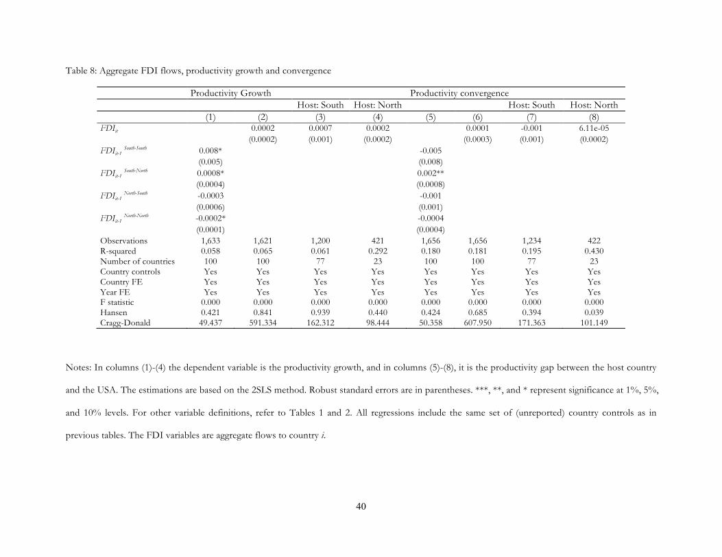
40

Table 8: Aggregate FDI flows, productivity growth and convergence

Productivity Growth Productivity convergence Host: South Host: North Host: South Host: North (1) (2) (3) (4) (5) (6) (7) (8) FDIit 0.0002 0.0007 0.0002 0.0001 -0.001 6.11e-05 (0.0002) (0.001) (0.0002) (0.0003) (0.001) (0.0002) FDIit-1

South-South 0.008* -0.005 (0.005) (0.008) FDIit-1

South-North 0.0008* 0.002** (0.0004) (0.0008) FDIit-1

North-South -0.0003 -0.001 (0.0006) (0.001) FDIit-1

North-North -0.0002* -0.0004 (0.0001) (0.0004) Observations 1,633 1,621 1,200 421 1,656 1,656 1,234 422 R-squared 0.058 0.065 0.061 0.292 0.180 0.181 0.195 0.430 Number of countries 100 100 77 23 100 100 77 23 Country controls Yes Yes Yes Yes Yes Yes Yes Yes Country FE Yes Yes Yes Yes Yes Yes Yes Yes Year FE Yes Yes Yes Yes Yes Yes Yes Yes F statistic 0.000 0.000 0.000 0.000 0.000 0.000 0.000 0.000 Hansen 0.421 0.841 0.939 0.440 0.424 0.685 0.394 0.039 Cragg-Donald 49.437 591.334 162.312 98.444 50.358 607.950 171.363 101.149

Notes: In columns (1)-(4) the dependent variable is the productivity growth, and in columns (5)-(8), it is the productivity gap between the host country

and the USA. The estimations are based on the 2SLS method. Robust standard errors are in parentheses. ***, **, and * represent significance at 1%, 5%,

and 10% levels. For other variable definitions, refer to Tables 1 and 2. All regressions include the same set of (unreported) country controls as in

previous tables. The FDI variables are aggregate flows to country i.

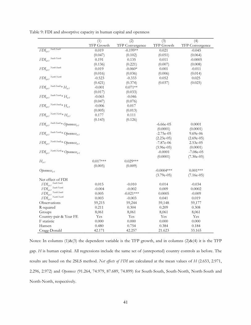
41

Table 9: FDI and absorptive capacity in human capital and openness

(1) (2) (3) (4) TFP Growth TFP Convergence TFP Growth TFP Convergence FDIijt-1

South-South 0.019 -0.199** 0.021 -0.045 (0.047) (0.102) (0.051) (0.064) FDIijt-1

South-North 0.191 0.135 0.011 -0.0005 (0.136) (0.221) (0.007) (0.008) FDIijt-1

North-South 0.019 -0.060* 0.001 -0.011 (0.016) (0.036) (0.006) (0.014) FDIijt-1

North-North -0.523 -0.333 0.052 0.025 (0.421) (0.374) (0.037) (0.025) FDIijt-1

South-South* Hit-1 -0.001 0.071** (0.017) (0.033) FDIijt-1

South-North* Hit-1 -0.065 -0.046 (0.047) (0.076) FDIijt-1

North-South* Hit-1 -0.006 0.017 (0.005) (0.013) FDIijt-1

North-North* Hit-1 0.177 0.111 (0.143) (0.126) FDIijt-1

South-South* Opennessit-1 -6.66e-05 0.0001 (0.0001) (0.0001) FDIijt-1

South-North* Opennessit-1 -2.75e-05 9.69e-06 (2.23e-05) (2.69e-05) FDIijt-1

North-South* Opennessit-1 -7.87e-06 2.53e-05 (3.96e-05) (0.0001) FDIijt-1

North-North* Opennessit-1 -0.0001 -7.08e-05 (0.0001) (7.30e-05) Hit-1 0.017*** 0.029*** (0.005) (0.009) Opennessit-1 -0.0004*** 0.001*** (3.79e-05) (7.16e-05) Net effect of FDI FDIijt-1

South-South 0.015 -0.010 0.014 -0.034 FDIijt-1

South-North -0.004 -0.002 0.009 0.0002 FDIijt-1

North-South 0.005 -0.021*** 0.0005 -0.009 FDIijt-1

North-North 0.003 -0.003 0.041 0.019 Observations 59,215 59,244 59,148 59,177 R-squared 0.211 0.304 0.209 0.308 Groups 8,061 8,061 8,061 8,061 Country-pair & Year FE Yes Yes Yes Yes F statistic 0.000 0.000 0.000 0.000 Hansen 0.480 0.754 0.384 0.184 Cragg-Donald 42.171 42.257 21.623 33.165

Notes: In columns (1)&(3) the dependent variable is the TFP growth, and in columns (2)&(4) it is the TFP

gap. H is human capital. All regressions include the same set of (unreported) country controls as before. The

results are based on the 2SLS method. Net effects of FDI are calculated at the mean values of H (2.653, 2.971,

2.296, 2.972) and Openness (91.264, 74.979, 87.689, 74.899) for South-South, South-North, North-South and

North-North, respectively.

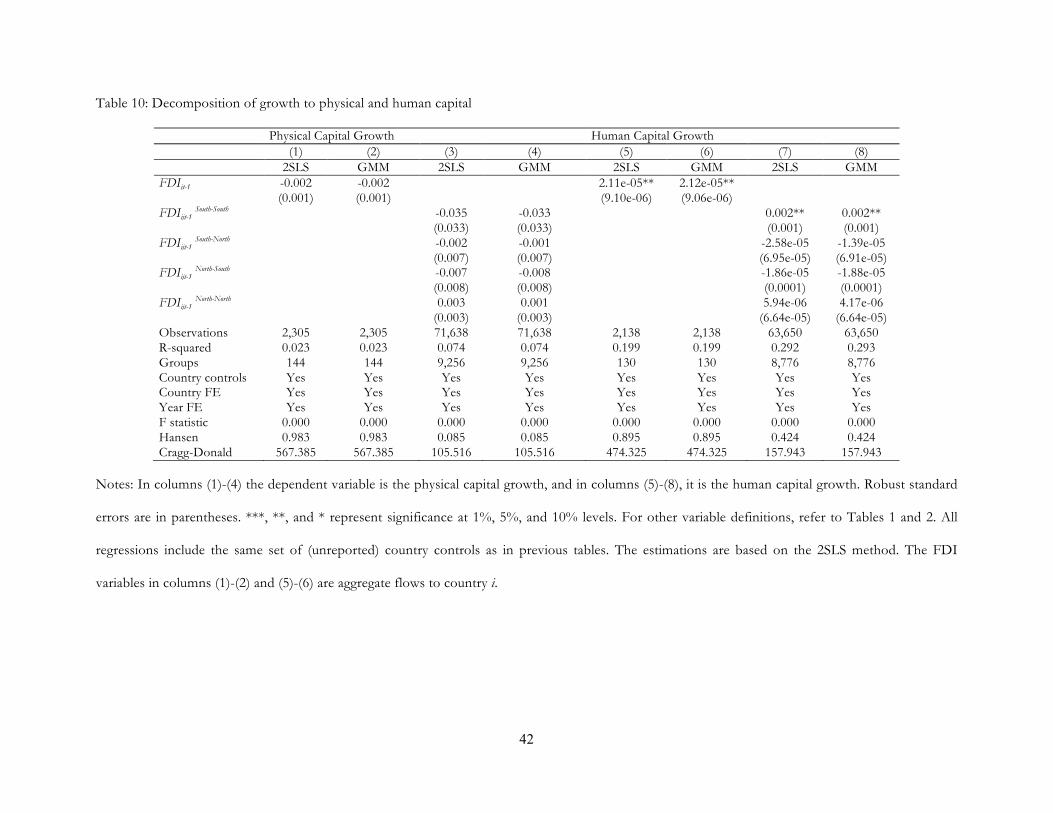
42

Table 10: Decomposition of growth to physical and human capital

Physical Capital Growth Human Capital Growth (1) (2) (3) (4) (5) (6) (7) (8) 2SLS GMM 2SLS GMM 2SLS GMM 2SLS GMM FDIit-1 -0.002 -0.002 2.11e-05** 2.12e-05** (0.001) (0.001) (9.10e-06) (9.06e-06) FDIijt-1

South-South -0.035 -0.033 0.002** 0.002** (0.033) (0.033) (0.001) (0.001) FDIijt-1

South-North -0.002 -0.001 -2.58e-05 -1.39e-05 (0.007) (0.007) (6.95e-05) (6.91e-05) FDIijt-1

North-South -0.007 -0.008 -1.86e-05 -1.88e-05 (0.008) (0.008) (0.0001) (0.0001) FDIijt-1

North-North 0.003 0.001 5.94e-06 4.17e-06 (0.003) (0.003) (6.64e-05) (6.64e-05) Observations 2,305 2,305 71,638 71,638 2,138 2,138 63,650 63,650 R-squared 0.023 0.023 0.074 0.074 0.199 0.199 0.292 0.293 Groups 144 144 9,256 9,256 130 130 8,776 8,776 Country controls Yes Yes Yes Yes Yes Yes Yes Yes Country FE Yes Yes Yes Yes Yes Yes Yes Yes Year FE Yes Yes Yes Yes Yes Yes Yes Yes F statistic 0.000 0.000 0.000 0.000 0.000 0.000 0.000 0.000 Hansen 0.983 0.983 0.085 0.085 0.895 0.895 0.424 0.424 Cragg-Donald 567.385 567.385 105.516 105.516 474.325 474.325 157.943 157.943

Notes: In columns (1)-(4) the dependent variable is the physical capital growth, and in columns (5)-(8), it is the human capital growth. Robust standard

errors are in parentheses. ***, **, and * represent significance at 1%, 5%, and 10% levels. For other variable definitions, refer to Tables 1 and 2. All

regressions include the same set of (unreported) country controls as in previous tables. The estimations are based on the 2SLS method. The FDI

variables in columns (1)-(2) and (5)-(6) are aggregate flows to country i.

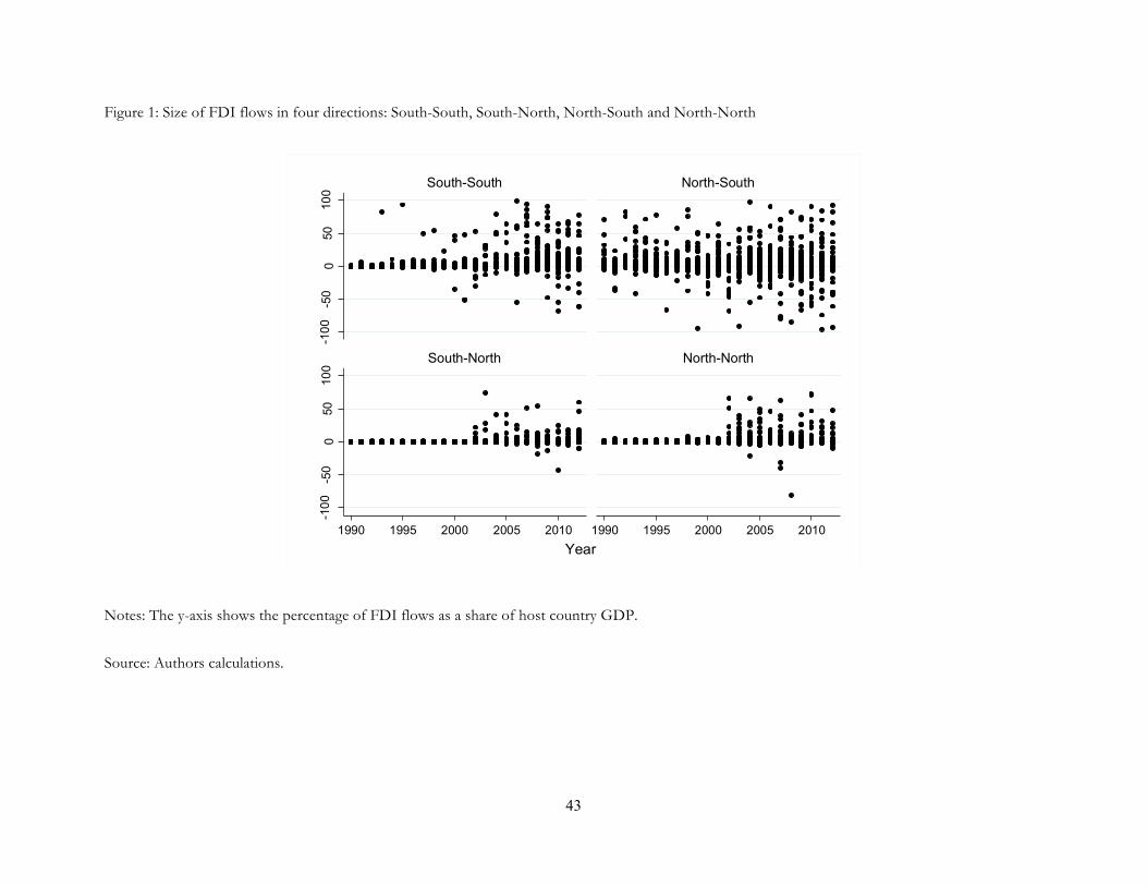
43

Figure 1: Size of FDI flows in four directions: South-South, South-North, North-South and North-North

Notes: The y-axis shows the percentage of FDI flows as a share of host country GDP.

Source: Authors calculations.

-100

-50

050

100

-100

-50

050

100

1990 1995 2000 2005 2010 1990 1995 2000 2005 2010

South-South North-South

South-North North-North

FDI t

o H

ost C

ount

ries'

GD

P (%

)

Year

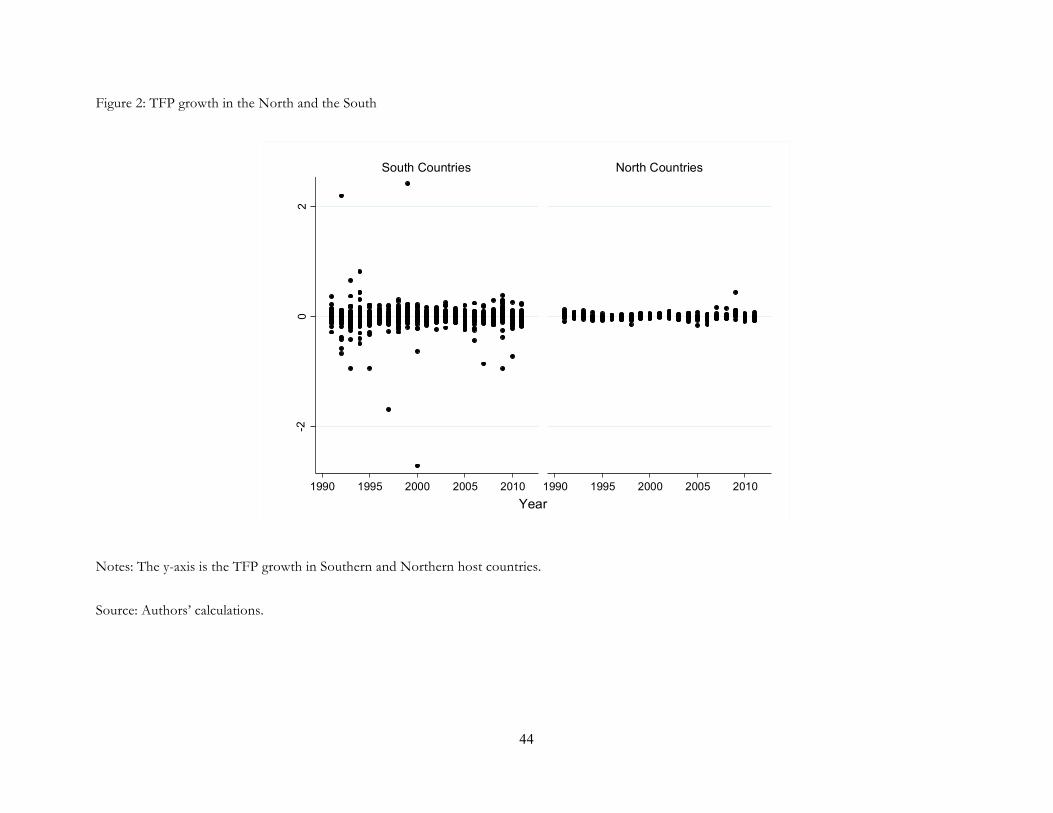
44

Figure 2: TFP growth in the North and the South

Notes: The y-axis is the TFP growth in Southern and Northern host countries.

Source: Authors’ calculations.

-20

2

1990 1995 2000 2005 2010 1990 1995 2000 2005 2010

South Countries North Countries

Pro

duct

ivity

Gro

wth

Year

45

Figure 3: Kernel density for relative TFP Gap

Notes: Kernel densities for the productivity gap of Northern and Southern host countries with the US.

Source: Authors’ calculations.

01

23

Den

sity

-3 -2 -1 0 1 2Relative Productivity Gap

Southern Countries Northern Countries